agb mass loss and stellar variability

Chapter 4

AGB mass loss and stellarvariability

In this chapter the relations between the mid-IR emission and pulsationproperties of O-rich AGB stars with known long period variability type arestudied. The analysis is made by using the tools developed in the previouschapter, and by modeling the sources with steady state spherically sym-metric radiative transfer. By fitting the IRAS Low Resolution Spectra ofthe circumstellar envelopes around each star, the thermal structure, opti-cal depth and mass loss rate are derived. The best fit parameters are thencorrelated with the central source variability type.

This work has been made in collaboration with Zeljko Ivezic, PrincetonUniversity, and has been presented at the International Workshop “Thechanges in Abundances in Asymptotic Giant Branch Stars”, held in Rome,September 16–18, 1999 (Marengo et al., 2000b). [Results of this analysisfinally published on Marengo et al. (2001)]

4.1 Long Period Variability in the AGB phase

On August 3, 1596, David Fabricius, an amateur astronomer native of Fries-land (The Netherlands) started a series of observations, aimed to determinethe position of a planet which he believed to be Mercury (it was, in fact,Jupiter). He used as reference point a nearby unidentified star of magni-tude 3 which, surprisingly, by August 21 had already increased to magni-tude 2. When the star faded and finally disappeared in October, Fabriciusassumed he had just observed a nova, and then forgot about it. On February15, 1609, he observed the star reappear, which was quite unusual. Fabricius,

70 AGB mass loss and stellar variability

who was a minister, unfortunately did not live to enjoy the appreciation ofits discovery, being murdered by a peasant whom he accused from the pulpitof having stolen one of the minister’s geese.1

The mysterious star was then forgotten, until Johann Fokkens, also ofFriesland, saw it again in 1638, determining that it was a variable star witha period of 11 months. The star was finally named Mira, which means “TheWonderful” by Johann Hevelius of Danzig, and o (omicron) Ceti by JohannBayer in 1603.

Today, Mira is taken as the prototype for a whole class of variable stars,with periods that can be as long as several hundred days, and whose lightcurves can be of several magnitudes in the optical. Mira, as other LongPeriod Variables (LPV), is an AGB star, characterized by pulsational insta-bilities in the atmospheric layers. Radial pulsations, with not fully under-stood dynamics, are responsible for periodic contraction and relaxation ofthe stellar photosphere, and thus for the variations of the stellar luminosity.

In the inner part of the LPV atmosphere, the passing shocks cause aperiodic modulation of the structure; in the upper layers the dissipation ofmechanical energy leads to a levitation, i.e. a density enhancement of up toseveral orders of magnitude, compared to an hydrostatic atmosphere. Bothof these effects can influence the formation of molecules and dust grains,and thus the mass loss properties of the star (Hofner, 1999).

If Long Period Variability is in some way one of the ingredients in dustformation processes in AGB stars, some correlation between the infraredproperties of LPVs, which are a function of dust production, and the pul-sational characteristics, should be expected. This is what this chapter aimsto explore.

4.1.1 Types of Long Period Variability

There are four main types of LPVs that are associated with the AGB phase:Miras (of which o Ceti is the prototype), Semiregulars of type “a” and “b”,and Irregulars of type “Lb”. According to the General Catalogue of VariableStars (GCVS, Kopolov et al. 1998), they are defined as follows:

Mira: long-period variables with characteristic late-type emission spectra(Me, Ce, Se) and light amplitudes from 2.5 to 11 magnitudes in V.Their periodicity is well pronounced, and the periods lie in the rangebetween 80 and 1000 days. Infrared amplitudes are usually less than

1see Hoffleit (1996) for an historical account on Mira discovery.

4.1 Long Period Variability in the AGB phase 71

in the visible, and may be less than 2.5 magnitudes; for instance, inthe K band they usually do not exceed 0.9 mag.

SRa: Semiregular variables of type a, which are late-type (M, C, S or Me,Ce and Se) giants displaying persistent periodicity and usually small(less than 2.5 magnitudes in V) light amplitude. Amplitudes andlight-curves generally vary, and periods are in the range 35–1200 days.Many of these stars differ from Miras only by showing smaller lightamplitudes.

SRb: Semiregular late-type (M, C, S or Me, Ce, Se) giants with poorlydefined periodicity (mean cycles in the range of 20 to 2300 days), orwith alternating intervals of periodic and slow irregular changes, andeven with light constancy intervals. Every star of this type may beassigned a certain main period, but the simultaneous presence of twoor more periods of light variation is observed.

Lb: Slow irregular variables of late spectral type (K, M, C and S), whichshows no evidence of periodicity, or any periodicity present is verypoorly defined and appears only occasionally. Lb stars are in generalpoorly studied, and may in fact belong to the semiregular type (SRb).

The length of the pulsational period, in the SR class, can be related tothe evolutionary phase of the pulsators along the AGB. Two independentstudies made by Jura & Kleinmann (1992) and Kerschbaum & Hron (1992)arrived at the conclusion that SRs having period P < 100d are characterizedby low mass loss rates (M ∼ 108 M¯ yr−1) and seem to be on the E-AGBphase. Semiregulars with longer periods have instead a higher mass loss,and presumably are in the TP-AGB. This classification is supported by thedetection of the s-element Tc in SRs with P & 100d (Little et al., 1987); Tcis otherwise not observed in most SRs with shorter period. Miras, on theother end, appears to be all in the TP-AGB phase.

However, it is clear from the above classification that the subdivisionbetween the various categories is rather thin, and can be easily biased bythe quality and frequency of the observations used for the construction ofvariable light curve.

According to Kerschbaum & Hron (1996), for example, SRa should beconsidered not as a class by themselves, but as a mixture of “intrinsic” Mirasand SRb. Jura & Kleinmann (1992) ignored this subdivision, arguing that,for an infrared selected sample, SRs can all be considered as a single class.


Fig. 4.1.— Light-curve of Mira (o Ceti) during several pulsational cycles.From the American Association of Variable Star Observers (AAVSO) web site(http://www.aavso.org).

A cautious approach is thus necessary, to avoid reaching erroneous con-clusions by analyzing samples of sources which are in general difficult todefine, and can be contaminated by pulsators in a different state.

4.1.2 Pulsation modes in Miras and SRs

An open problem concerning the dynamics of pulsations in Long periodVariables is the determination of the pulsational mode. This is somewhatsurprising, since the ratio of the fundamental mode and first overtone periodin an AGB variable is larger than 2 (Wood & Sebo, 1996). Any reasonableestimate of the radius and mass of an LPV should thus be enough to deter-mine the pulsational mode. This is unfortunately untrue, since a number ofobservational difficulties can make this measurement rather awkward, andstill leave the problem open.

A mass of 1 M¯ is usually adopted in these computations, based on kine-matics studies of LPVs in the Galaxy. This value, however, tends to favorfirst overtone pulsations over fundamental mode, thus biasing the measure-ment. The determination of the angular radii, also suffers of serious prob-

4.2 A sample of Mira, Semiregular and Irregular variables 73

lems, mainly due to the wavelength dependence of the measured diameters,which requires accurate model atmosphere predictions to be usable. Thedetermination of the distance is also uncertain, even after the HIPPARCOSmission, which provides a large set of reasonable parallaxes. The theoreticalmodels used to analyze the pulsations are also a source of confusion, beingnot at all clear if classical pulsation theory is applicable to LPVs, or if morerefined models are required (Tuchman, 1999).

Fourier analysis of LPV light-curves, can also give direct informationon the pulsational mode. An extensive analysis of Mira itself (Barthes &Mattei, 1997) showed a main period of 332.9 days, which is interpreted asfirst overtone, and a second periodicity of 1503.8 days associated to the fun-damental mode. Other analysis of Mira stars made with similar techniquesfound pulsations which can be interpreted as first overtone pulsation modes.Semiregulars, on the contrary, are often associated to combinations of thefirst overtone with higher pulsational modes.

Wood et al., (1999), however, by analyzing the relative position in theperiod luminosity plane of LMC Miras and SRs in the MACHO database,found five distinct period-luminosity sequences. These sequences allowedthem to conclude that Miras are unambiguously fundamental mode pul-sators, while SRs pulsates on a combination of the various overtones.

Even though different analyses are producing contradicting answers, acommon result seems to be that SRs appear to pulsate as a combinationof higher overtones with respect to Miras. More data and a better under-standing of the physics of pulsations in the perturbed atmospheres of vari-able AGB, are still necessary to provide a reliable answer on this importantquestion.

4.2 A sample of Mira, Semiregular and Irregularvariables

In order to test the link between AGB long period variability and massloss, we have selected a sample of LPVs for which the IRAS mid-IR spectrawere available. This sample is characterized in the next section, and thenanalyzed from the point of view of the mid-IR properties in the LRS spectralregion, by studying its mid-IR colors and the shape of the silicate feature.


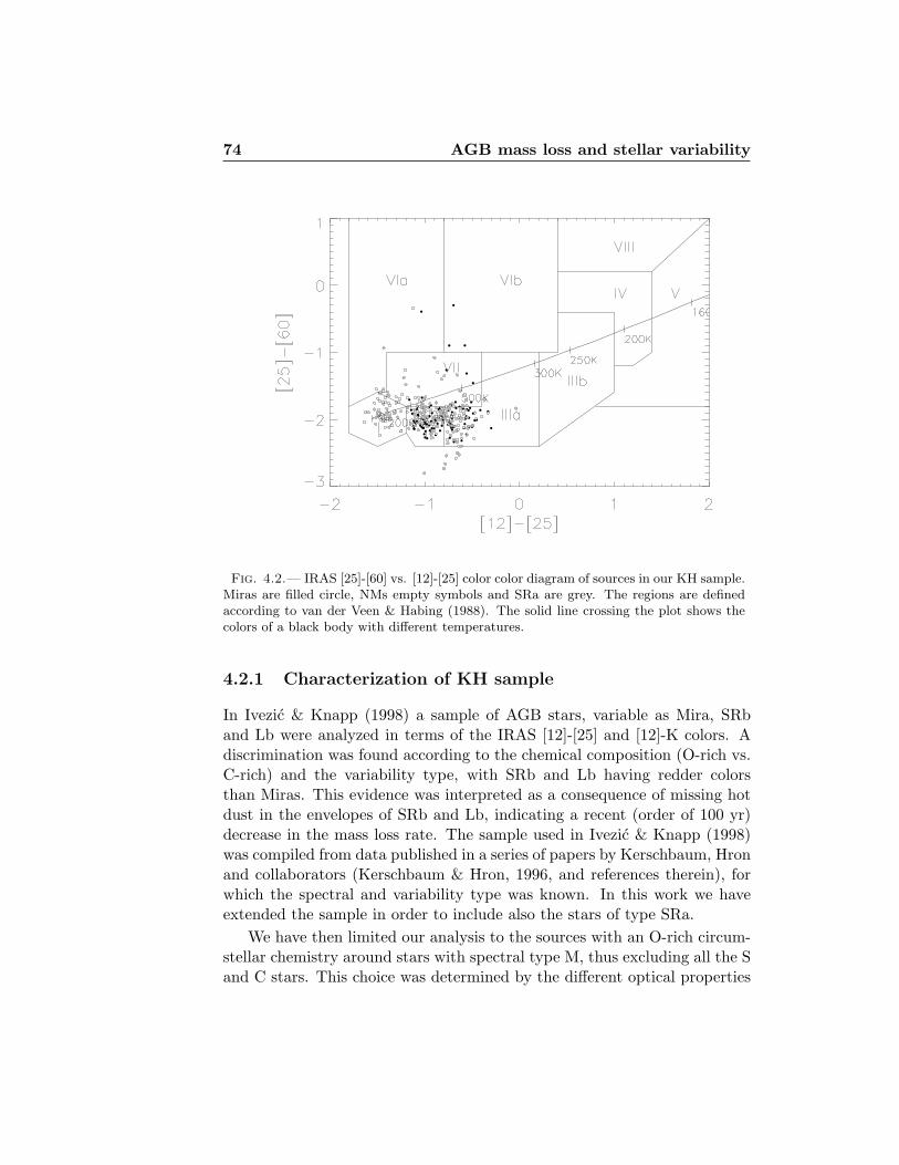
Fig. 4.2.— IRAS [25]-[60] vs. [12]-[25] color color diagram of sources in our KH sample.Miras are filled circle, NMs empty symbols and SRa are grey. The regions are definedaccording to van der Veen & Habing (1988). The solid line crossing the plot shows thecolors of a black body with different temperatures.

4.2.1 Characterization of KH sample

In Ivezic & Knapp (1998) a sample of AGB stars, variable as Mira, SRband Lb were analyzed in terms of the IRAS [12]-[25] and [12]-K colors. Adiscrimination was found according to the chemical composition (O-rich vs.C-rich) and the variability type, with SRb and Lb having redder colorsthan Miras. This evidence was interpreted as a consequence of missing hotdust in the envelopes of SRb and Lb, indicating a recent (order of 100 yr)decrease in the mass loss rate. The sample used in Ivezic & Knapp (1998)was compiled from data published in a series of papers by Kerschbaum, Hronand collaborators (Kerschbaum & Hron, 1996, and references therein), forwhich the spectral and variability type was known. In this work we haveextended the sample in order to include also the stars of type SRa.

We have then limited our analysis to the sources with an O-rich circum-stellar chemistry around stars with spectral type M, thus excluding all the Sand C stars. This choice was determined by the different optical properties


of O-rich and C-rich dust. The 9.8 µm silicate feature of O-rich envelopes,as shown in section 3.3.3, makes the spectrum of these sources particularlysensitive to small variations of the physical parameters and temperaturestructures of the envelopes. The almost featureless opacities of amorphouscarbon dust present in C-rich envelopes, on the other end, are much lessdependent on changes in the dust grain temperature distribution. For thisreason, fitting mid-IR spectra (and in particular the inner envelope temper-ature T1) is potentially more accurate in the case of oxidic dust.

Of all the sources in the original Kerschbaum & Hron (1996) list, we haveexcluded also the ones for which the IRAS LRS was unavailable, ending witha list of 432 sources (KH sample, hereafter). In our KH sample 96 are Miras,48 SRa, 140 SRb and 58 Lb. We have then combined the SRa, SRb and Lbin a single sample of 246 non-Miras (NMs).

To test the possibility that SRa are a spurious class containing a mix-ture of Mira and SR variables, we have cross correlated the results with aseparate sample of SRa sources alone, as a precaution to check if our NMsare “contaminated” by erroneous classified Miras.

The distribution of KH sources in the IRAS color color diagram describedin section 3.3.2 is shown in figure 4.2. Note that most of the sources aredistributed in regions II and IIIa of the diagram (containing variable starswith young circumstellar envelopes). NMs, however, are also present inregion I, where sources without a circumstellar shell (or, rather, having anoptically thin one) are located. We have finally cross correlated our samplewith the General Catalogue of Variable Stars (GCVS, Kopolov et al. 1998),in order to derive the pulsational period of all sources, when available.

Our sample contains 57 SRs with P < 100d and 130 with P & 100d

which, according to Jura & Kleinmann (1992) and Kerschbaum & Hron(1992) should be in the Early- and TP-AGB phase, respectively. The anal-yses performed in the following sections are then checked against this sub-division, in order to verify that any eventual difference between Miras andNMs is due to the pulsational mode, and not to the evolutionary status ofthe sources.

Due to the nature of the samples from which our KH list is derived,and in particular to the limitations in the IRAS catalog, affected by sourceconfusions in the galactic plane, our sample is not statistically complete.Nevertheless, it provides significant indications for the whole class of O-richgalactic AGB variables.


Fig. 4.3.— Silicate color diagram of sources in KH sample. Miras are filled circle, NMsempty symbols and SRa are grey.

4.2.2 Mid-IR colors and variability

Preliminary information on the physical and chemical status of dusty cir-cumstellar envelopes can be obtained by using a suitable photometric systemtuned for mid-IR observations, as shown in chapter 3.

As for the test sources used to calibrate our mid-IR color color diagrams,we have derived the photometry in the 8.5, 9.8, 12.5 and 18.0 “standard”gaussian filters by convolving the LRS spectra with the filter profiles, asexplained in section 3.3.2. Since all KH sources are O-rich, the “silicatecolor” diagram is the natural choice to probe the properties of the dustthermal emission in the mid-IR. The plot, shown in figure 4.3, brings intoevidence that NMs, and among them most of the SRa, are distributed alongthe black body line, with a large spread in the [8.5]-[12.5] color. Miras,on the contrary, are clumped above the black body, with −0.1 . [8.5]-[12.5]. 0.5. This region, as shown in figure 3.10, is mostly populated by envelopeswith intermediate optical depth (1 . τV . 30).

The [8.5]-[9.8] color shows that Miras have a tendency to have a stronger9.8 µm silicate feature, while NMs and especially SRa tends to be found


Fig. 4.4.— Dust continuum color diagram of sources in KH sample. Miras are filledcircle, NMs empty symbols and SRa are grey.

closer to the black body, where featureless 1n class spectrum are usuallylocated. The absence of a complete separation between Miras and NMs,does not allow to discuss the detailed properties of the silicate feature in thetwo groups on the basis of the [8.5]-[9.8] color alone. A specific test on theshape of the silicate feature requires the analysis of the full LRS spectra, asdescribed in the next section.

The absence of sources below the black body, in the region otherwiseoccupied by the 3n class of objects, indicates that the optical depth of KHsources is never high enough to produce a silicate feature self absorbed.

The “thermal continuum” diagram [12.5]-[18.0] vs. [8.5]-[12.5], shown infigure 4.4, does highlight a difference between Miras and NMs, as NMs havean average redder [12.5]-[18.0] color. This cannot be due to a higher opticaldepth of NM envelopes, which would affect also the “silicate feature” colordiagram; it suggests instead the presence of colder circumstellar dust aroundNMs, as found in Ivezic & Knapp (1998). SRa have a distribution similarto the NMs, but [8.5]-[12.5] & −0.1 (as for the Miras).


Fig. 4.5.— Distribution of the [12.5]-[18.0] excess colors for Miras (dashed line), NMs(solid line) and SRa (dotted line) for the KH sample.

A quantitative test is provided by the histogram in figure 4.5, and sum-marized in table 4.1. The histogram plots the distribution of Miras, SRa andNMs in the [12.5]-[18.0] color excess, defined for each source as the differencebetween its color and the color of a black body with the same [8.5]-[12.5]color temperature. The mean value for this quantity is ∼ 0.11 for Miras,∼ 0.32 for NMs and ∼ 0.33 for SRa. The 0.2 magnitude difference betweenthe Miras and NMs distribution is larger than the dispersion of the twosamples, measured by the variance σ ' 0.18 of both Miras and NMs. Wetested this result with a Student’s t-test for the mean values, finding that thedifference between the two population is indeed statistically significant (seetable 4.1 for further details). We then performed the same analysis uponthe two SR subsamples with P < 100d and P & 100d, finding a similar colorexcess in the two cases (0.36 and 0.30 magnitudes), which is not significantwith respect to the 0.01 Studen’t t-test significance level.

This two tests suggest that, from the point of view of the color temper-ature of their circumstellar dust, Miras and NMs are two different popu-lations. Among the SR sources, the physical characteristics of the circum-


Table 4.1 [12.5]−[18.0] color excess.

Sample Median [mag] Mean [mag] σ [mag] N sources

Mira 0.10 0.11 0.18 96NM 0.34 0.32 0.18 246SRa 0.37 0.33 0.19 48SR (P < 100d) 0.37 0.36 0.17 57SR (P & 100d) 0.32 0.30 0.20 130

Significance of statistical tests

Sample F-test t-test Result at 0.01 significancea

Mira vs. NM 0.90 6 · 10−20 Same σ and different meanSRa vs. Mira 0.70 2 · 10−10 Same σ and different meanSRa vs. NM 0.60 0.71 Same σ and meanSR P<100d vs. P&100d 0.16 0.05 Same σ and mean

a Samples have different σ if the variance F-test returns a significance of 0.01 or smaller, anddifferent mean values if Student’s t-test returns a significance of 0.01 or smaller

stellar envelopes are instead homogeneous across all pulsational periods.Assuming the validity of the Kerschbaum & Hron (1992) correlation be-tween pulsational periods and AGB evolution, this is suggestive that SRsform similar circumstellar envelopes in the Early- and TP-AGB phases. Thesimilarity of SRa with NMs, may indicate that there is not a large contam-ination of Miras in the KH sample.

4.2.3 Variability and the main silicate feature

The shape and characteristics of the 9.8 µm silicate feature observed inthe spectra of O-rich AGB circumstellar envelopes is in general affectedby many different factors, intrinsic as the grain chemical composition, sizedistribution, structure (crystalline of amorphous) and degree of processing(e.g. annealing), or extrinsic as the radiative transfer effects due to theenvelope optical depth, thermal structure and geometry.


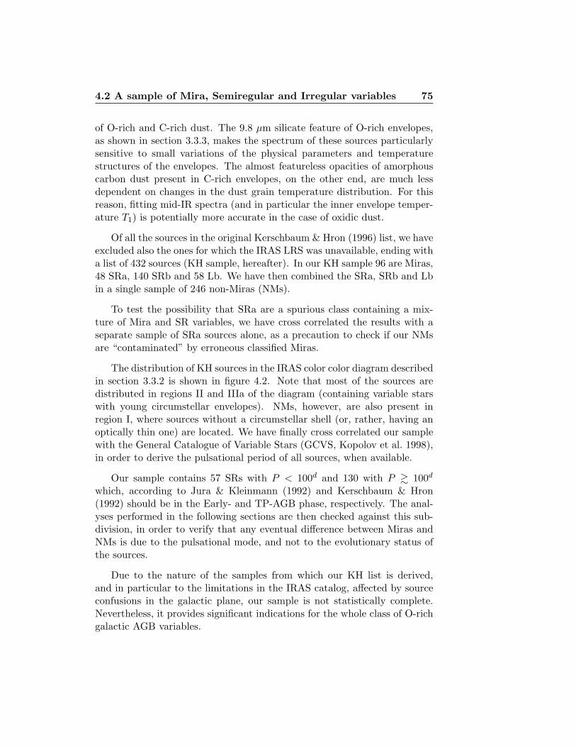
Fig. 4.6.— Distribution of the 10 µm silicate feature peak of KH sources. Dashed lineis for Miras distribution, solid line for NMs and dotted line for SRa.

Little-Marenin & Little (1990) first tried to classify a large sample ofO-rich AGB variables from the point of view of their silicate feature in theIRAS LRS spectra. They found that their sample of SR and Irregularswas showing a narrower silicate feature, shifted to the red, compared to theMiras. A similar analysis was performed by Hron et al. (1997) with largerstatistics, and taking into account the dust continuum emission by fittingit with a separate black body. This later work confirmed the differencesbetween the two classes, finding a shift of about 0.3 µm in the peak position.

In order to probe the KH sources in terms of the shape of their silicatefeature, we have fitted each individual IRAS LRS with the best 5 degreepolynomial in the 9-11 µm wavelength range. The fitting procedure removesthe effect of noise and eventual secondary features, producing “smooth”spectra where the position of the maximum can be easily recognized. Thewavelength of the maximum of the best fit polynomial in the given intervalis then assumed to be the position of the “true” silicate peak.

With this technique we measured the position of the silicate peak of 85Miras and 162 NMs; for the remaining sources (11 Miras and 84 NMs) the


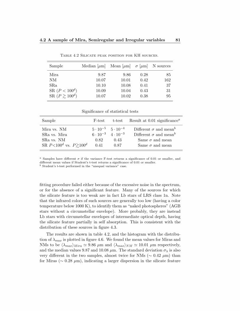
Table 4.2 Silicate peak position for KH sources.

Sample Median [µm] Mean [µm] σ [µm] N sources

Mira 9.87 9.86 0.28 85NM 10.07 10.01 0.42 162SRa 10.10 10.08 0.41 37SR (P < 100d) 10.09 10.04 0.43 31SR (P & 100d) 10.07 10.02 0.38 95



Mira vs. NM 5 · 10−5 5 · 10−4 Different σ and meanb

SRa vs. Mira 6 · 10−3 4 · 10−3 Different σ and meanb

SRa vs. NM 0.82 0.43 Same σ and meanSR P<100d vs. P&100d 0.41 0.87 Same σ and mean

a Samples have different σ if the variance F-test returns a significance of 0.01 or smaller, anddifferent mean values if Student’s t-test returns a significance of 0.01 or smaller.b Student’s t-test performed in the “unequal variance” case.

fitting procedure failed either because of the excessive noise in the spectrum,or for the absence of a significant feature. Many of the sources for whichthe silicate feature is too weak are in fact Lb stars of LRS class 1n. Notethat the infrared colors of such sources are generally too low (having a colortemperature below 1000 K), to identify them as “naked photospheres” (AGBstars without a circumstellar envelope). More probably, they are insteadLb stars with circumstellar envelopes of intermediate optical depth, havingthe silicate feature partially in self absorption. This is consistent with thedistribution of these sources in figure 4.3.

The results are shown in table 4.2, and the histogram with the distribu-tion of λmax is plotted in figure 4.6. We found the mean values for Miras andNMs to be 〈λmax〉Mira ' 9.86 µm and 〈λmax〉NM ' 10.01 µm respectively,and the median values 9.87 and 10.08 µm. The standard deviation σλ is alsovery different in the two samples, almost twice for NMs (∼ 0.42 µm) thanfor Miras (∼ 0.28 µm), indicating a larger dispersion in the silicate feature


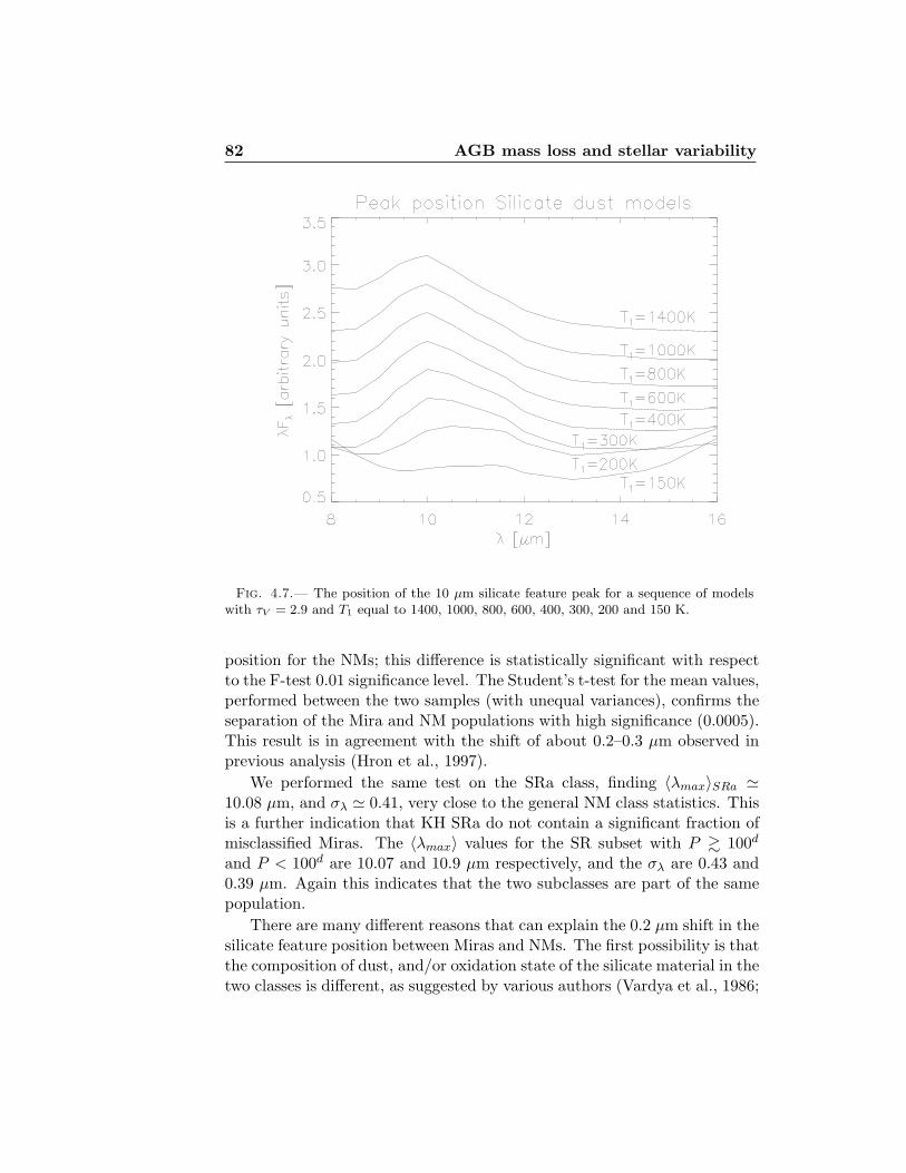
Fig. 4.7.— The position of the 10 µm silicate feature peak for a sequence of modelswith τV = 2.9 and T1 equal to 1400, 1000, 800, 600, 400, 300, 200 and 150 K.

position for the NMs; this difference is statistically significant with respectto the F-test 0.01 significance level. The Student’s t-test for the mean values,performed between the two samples (with unequal variances), confirms theseparation of the Mira and NM populations with high significance (0.0005).This result is in agreement with the shift of about 0.2–0.3 µm observed inprevious analysis (Hron et al., 1997).

We performed the same test on the SRa class, finding 〈λmax〉SRa '10.08 µm, and σλ ' 0.41, very close to the general NM class statistics. Thisis a further indication that KH SRa do not contain a significant fraction ofmisclassified Miras. The 〈λmax〉 values for the SR subset with P & 100d

and P < 100d are 10.07 and 10.9 µm respectively, and the σλ are 0.43 and0.39 µm. Again this indicates that the two subclasses are part of the samepopulation.

There are many different reasons that can explain the 0.2 µm shift in thesilicate feature position between Miras and NMs. The first possibility is thatthe composition of dust, and/or oxidation state of the silicate material in thetwo classes is different, as suggested by various authors (Vardya et al., 1986;

4.3 Modeling the mid-IR spectra 83

Little-Marenin & Little, 1988; Onaka et al., 1989; Sloan & Price, 1998). Asecond explanation is that the grain size distribution may be different. Thispossibility has been explored by Simpson (1991). The results of her work,however, show that to produce a noticeable change in the silicate feature ofthe envelope spectra, a variation in the dust grain size of at least a factor 7is required. As argued by Hron et al. (1997), current dynamical models fordust driven winds (Hofner & Dorfi, 1997) indicate that such large variationsin the particle size are unlikely to be produced.

There is, however, a third possibility, that is to invoke radiative transferas the cause of the peak shift. Envelopes with fixed optical depth τV anddecreasing dust temperature emit an increasing fraction of their thermalradiation at longer wavelengths. This translates in “flat” spectra in whichthe contribution from the silicate feature, gradually self absorbed, is boundto disappear, until the thermal continuum produces a “bump” in the spec-trum which can be interpreted as a shift in the peak of the feature. Thiseffect is shown in figure 4.7 for a sequence of models with τV ' 2.9 andgradually decreasing dust temperature T1. Note how the shift becomes verypronounced; this suggests that cold envelopes would have a much larger dis-persion in the λmax distribution (as in fact is observed for our NM variables),than envelopes with hotter dust.

4.3 Modeling the mid-IR spectra

To quantify the color temperature difference between KH Miras and NMs,and separate the effects of dust thermal structure and optical depth, wehave estimated T1 and τV for each KH source by fitting its LRS spectrum.The adopted best fit procedure is based on χ2 minimization of the indi-vidual spectra with a series of DUSTY models, computed as described insection 3.2. Details on the fitting technique are given in section 4.3.2, andthe efficiency in obtaining a good quality fit is discussed in 4.3.3.

As radiative transfer modeling with DUSTY requires to specify the ge-ometry, dust radial density profile and grain size distribution, the dust massloss rate needed to produce each model envelope is fully characterized by acertain combination of model parameters. The explicit relation between bestfit parameters and Md is given in section 4.4, where the statistical distribu-tion of the dust temperature structure and optical depth is also discussed,in terms of the Mira vs. NM dichotomy suggested in the previous sections.


Fig. 4.8.— Silicate color diagram of KH sources with DUSTY models having 2500 KEngelke central source with 10% SiO absorption. Models with T1 equal to 100, 150, 200,300, 400, 600, 800, 1000 and 1400 K are plotted.

4.3.1 Model parameter space

Since our KH sample contains only O-rich sources, and has circumstellarenvelopes with oxidic dust, we have adopted the full grid of models computedin section 3.2 with the Ossenkopf et al. (1992) dust. The models were runwith “standard” MRN grain size distribution, and nd(r) ∝ r−2 radial densityprofile (steady mass loss during the phase in which the current envelope wasproduced). The inner radius R1 was fixed by the choice of the inner shelltemperature T1, and the outer envelope radius was scaled as R2 ' 1000 ·R1.

As for the brightness energy distribution of the central star, we havetested both the “standard” 2000 K black body, and the Engelke functionwith 10% SiO absorption described in section 3.2.2. Even though the En-gelke + SiO function provides the best fits for dustless sources with “nakedphotosphere” and envelopes characterized by a very low optical depth, wefound that a standard black body is in general a better choice for AGBenvelopes with τV ∼ 1. As shown in figure 4.8 and 4.9: models computedwith the Engelke + SiO function have the tendency to produce LRS spectra


Fig. 4.9.— Silicate color diagram of KH sources with DUSTY models having 2000 KPlanck black body central source. Models with T1 equal to 100, 150, 200, 300, 400, 600,800, 1000 and 1400 K are plotted.

with an excessive strength of the 10 µm silicate feature (resulting in toohigh [8.5]-[9.8] color). Models with the black body curve, on the contrary,can better reproduce the distribution of HK sources in the color color plane.For this reason, the analysis which follows has been entirely made using theDUSTY models with Planck black body central source.

A fine logarithmic grid of models with τV from 10−3 to 231, and T1 from100 to 1400 K was used, with 60 steps in τV and 31 in T1, in order to providethe necessary precision in the best fit parameters. Note in figure 4.9 how thecoldest dust family of models (track with T1 ' 100 K) is totally inadequateto fit any source in the KH sample. The coldest models able to provide agood fitting of the sources, have T1 ' 150 K, which can be assumed as arough estimate of the minimum inner shell temperature in our sample ofAGB envelopes.

A subset of models with T1 restricted to the interval 630–1400 K (“hotdust” models hereafter) was then extracted from the full set, in order to testwhether “cold dust” models with lower T1 are really necessary to improvethe fitting of certain classes of spectra.


4.3.2 Fitting technique

The best fit models for each source in our sample were found with a χ2

minimization routine applied to the source and model spectra in the IRASLRS wavelength range only. Even though the IRAS point source photometrywas available for all sources, and easily derived for the models, we decidedto restrict the fitting procedure to the 7–23 µm interval. This decision wasmade in order to avoid galactic cirrus contamination at longer wavelengths,and the phase dependence of optical and near-IR photometry with the LPVof the sources.

For each source in the sample, the models were individually renormalizedto match the absolute flux scale of the source LRS. The normalization factorα of each model was computed by least square minimization of the distancebetween model and source:

α =∑N

i=1

(λiF

Sν · λiF

Mν

)∑N

i=1 (λiFMν )2

(4.1)

where λiFSν is the source spectral energy distribution (the IRAS LRS) and

α · λiFMν the (renormalized) model, rebinned on the LRS wavelength grid,

on which the summation index i runs. The χ2 variable of each source-modelpair was then defined as:

χ2 =1

N − 2

N∑

i=1

[λiF

Sν (λi)− α · λiF

Mν (λi)

]2

σ2S (λi) + σ2

M (λi)(4.2)

The error σS of the IRAS LRS was derived by subtracting the LRSwith a smoothed version of themselves, while the error σM was estimatedas the difference between the two closest models in the parameter space.The χ2 variable was finally divided by the number of degrees of freedomN − 2, where N = 80 is the number of wavelengths, and 2 are the fittingparameters measured in the fit (τV and T1). Each source was then assignedto its best fit model, providing the minimum value of the χ2 variable.

As a consistency test for our fitting procedure, we have simulated a setof LRS spectra with known T1 and τV , covering the whole model parameterspace, by introducing gaussian noise to our DUSTY model grid. The syn-thetic spectra were then fitted by using the same original models, withoutnoise. The results are shown in figure 4.10 for S/N = 10 and S/N = 5 (thefirst case is the typical one for our sources, and the second corresponds tothe most noisy sources in the sample). Each circle in the plots represent a


Fig. 4.10.— Test diagram of χ2 fitting procedure. Artificial gaussian noise have beenadded to the full grid of models and to the resulting spectra. This produced “noisyfied”spectra, with S/N = 10 (left) and 5 (right), which have been fitted using the unmodifiedgrid. Each circle represents one point of the model grid for which the correspondent“noisyfied” model have been successfully fitted. Empty spaces in the regular grid patterncorrespond to models not correctly fitted, as a consequence of the added noise.

point in the model grid; missing points are “noisyfied” models which havenot been fitted correctly by our procedure.

The figure shows that increasing noise can reduce the effectiveness of ourprocedure, but within the limits of our sample is not likely to introduce biasesin the fit results. The missing points in the grid are distributed uniformly,at least in the regions where the physical parameters of KH sources areexpected to fall. Sources with τV . 0.02 are likely to have their optical depthoverestimated, due to constraints in the numerical accuracy of the models,which for very low τV are practically indistinguishable. The distribution ofthe incorrectly identified models in T1 is completely uniform, validating ourprocedure for fitting this parameter.

4.3.3 Fit results

The quality of our fits is estimated by the value of the best χ2 variable.As shown in figure 4.11, best fit models with χ2 . 3 are in general able toreproduce the source LRS with great accuracy, matching the position of thetwo silicate features (at 9.8 and 18 µm), their relative height and width, andthe slope of the continuum emission. Fits with 3 . χ2 . 5, are still good,even though some peculiarity of the silicate feature are not exactly repro-duced. The continuum slope, however, is still well modeled, and the smalldiscrepancies are in most cases due to the presence of secondary features,or the unusual width of the source LRS silicate feature, in the 13–14 µm


a) b)

c) d)

Fig. 4.11.— IRAS Low Resolution Spectra of Mira and NM sources (solid line) withbest fit models (dashed dotted line). In panel a the SRb star TY Dra is fitted with a colddust model (T1 ' 370 K), resulting in a very small χ2. If the dust temperature is limitedto the range 640–1400 K (as in the “hot dust” models), the fit is unable to reproducethe source spectral energy distribution (panel b). Panel c and d shows good quality fitsof a Miras with relatively hot dust (T1 ' 825 K) and a SRs with very low inner shelltemperature (T1 ' 270 K).

range, which cannot be fitted with the Ossenkopf et al. (1992) opacity. Abetter fit of these models probably requires a larger set of opacities, allow-ing variations in the dust composition. Models with χ2 & 5, on the otherhand, show more serious problems, as the wrong fit of dust continuum emis-sion, or failure in the fitting routine convergence, due to insufficient S/Nin the source LRS. The best fit parameters obtained for these sources areless reliable, since a better fitting may require radically different opacities,or changes in the envelope geometry, such as the presence of multiple dustshells.

The statistics of the best fit χ2 for our KH sources is shown in table 4.3.The left side of the table reports the number of sources having χ2 largerthan 3, 5 and 10 in the Miras, NMs, SRa and period selected SRs, fitted

4.4 Correlation between mass loss rate and shell temperature 89

Table 4.3 Sources which cannot be fitted with χ2 better than 3, 5and 10.

all models hot modelsSample χ2&3 χ2&5 χ2& 10 χ2&3 χ2&5 χ2& 10

Mira 35% 19% 3% 42% 31% 12%NM 18% 6% 1% 54% 27% 22%SRa 21% 4% 2% 33% 12% 4%SR (P<100d) 18% 5% 0% 67% 42% 21%SR (P&100d) 21% 7% 2% 48% 18% 6%

with the full grid of models. The right side present the same statistics, butwith the use of the “hot dust” family of models (models with T1 & 640 K).Notice that all NM sources shows a significant improvement in the qualityof their fits when “cold dust” models (T1 . 640 K) are allowed (compare,e.g. panels a and b of figure 4.11), while Miras can be equally well fittedusing “hot dust” models alone. This is a further evidence that the class ofNM is more likely to show colder envelopes than the average Mira source.

4.4 Correlation between mass loss rate and shelltemperature

The statistical distribution of the best fit parameters for our KH sample canbe analyzed to test the separation between Miras and NMs suggested by thedifferent colors and silicate feature position.

This statistical analysis is limited to sources with χ2 better than 10, inorder to prevent unreliable fits to bias our conclusions. This restriction isaimed to exclude the sources in which the continuum emission is not exactlyreproduced by the model, and thus the fitting procedure is suspected to haveconverged on mistaken best fit parameters. The excluded sources are 19%of the Miras, and 6% of the NMs.

This precautional measure, however, does not seem to affect the statis-tical validity of our results: similar tests performed on the whole sampleyielded the same conclusions, within the approximations of our technique.


Fig. 4.12.— Distribution of the best fit optical depth τV for Miras (dashed line), NMs(solid line) and SRa (dotted line).

4.4.1 Distribution of envelope optical depths

Figure 4.12 shows the statistical distribution of the best fit optical depth forour KH sources. The histogram appears to be bi-modal, with a double-peakdistribution centered at τV ∼ 1 and τV ∼ 25 respectively. NMs appears tobe distributed mainly in the low τV bin, while Miras, although present inboth categories, are mainly concentrated in the high optical depth bins. SRaappears to be equally distributed in the two categories, with a prevalencefor low optical depths.

This diagram reflects a well known characteristic of LPVs: Miras ingeneral possess higher optical depths than non-Miras, which on the contraryare in general brighter optically. From the analysis of our sample it is difficultto decide if the separation between the low and high τV distribution isstatistically significant: larger statistics and a more accurate fit with betteropacities is probably necessary to validate this result. The different averageoptical depth of the two main classes (Mira and NM), is however largeenough to be confirmed by the statistical tests reported in table 4.4.

Note that the Student’s t-test in table 4.4 underestimates the differencebetween the various populations, since it analyses the mean value assuming


Table 4.4 Distribution of best fit τV for KH sources.

Sample Median Mean σ N sources (χ2 . 5)

Mira 23.1 25.4 21.8 81 (81%)NM 1.2 16.6 25.9 232 (94%)SRa 2.3 20.9 25.1 46 (96%)SR (P < 100d) 0.8 10.5 25.8 54 (95%)SR (P & 100d) 1.5 20.2 26.2 121 (93%)



Mira vs. NM 0.08 7 · 10−3 Same σ and different meanSRa vs. Mira 0.28 0.30 Same σ and meanSRa vs. NM 0.83 0.29 Same σ and meanSR P<100d vs. P&100d 0.92 0.02 Same σ and mean

a Samples have different σ if the variance F-test returns a significance of 0.01 or smaller, anddifferent mean values if Student’s t-test returns a significance of 0.01 or smaller.

a gaussian distribution. This is of course not valid for the bimodal distribu-tions shown in figure 4.12. A much better comparison between the differentsubsamples is given by the median values of the best fit τV , which are closerto the modal value for each sample. In this case, SRa appears to be moresimilar to NMs than to Miras, even though the Student’s t-test cannot de-cide on the basis of the mean value. This confirms that our SRa does nothave a large contamination of Miras. The two subclasses of NMs appearsto have similar optical depths, even though short period NMs tends to havelower τV .

4.4.2 Distribution of inner shell temperatures

If the segregation between Miras and NMs is related to an intrinsic differencein the underlying mass loss mechanism, a correlation between the best fitτV and T1 should be expected. This is shown in figure 4.13, where the KHsources appear distributed in a strip crossing the diagram. Even though


both classes of sources are present along the whole sequence, Miras tend toaggregate at the top of the strip, with higher optical depths and T1. NMs,on the contrary, have in general lower T1 and τV . A discontinuity in thedistribution of the sources for T1 ' 500 K, suggests to divide the diagramin 4 separate regions, labeled counter-clockwise from I to IV, with most ofthe sources in quadrant I and III only. A quantitative distribution of thevarious subclasses in the four quadrants is given in table 4.5.

The sequence observed in figure 4.13 can be explained by assuming thatlow T1 are the product of envelope expansion, after the interruption of themass loss rate. At the end of an intense dust production phase, an envelopestarting at the inner radius Rc (dust condensation radius) will have a “steadystate” radial profile nd(r) ' nd(Rc) · (Rc/r)2. If the dust production stops,the envelope would detach, expanding at a radius R1 = Rc +vet, where ve isthe expansion velocity and t the time since the envelope detachment. Fromequations 2.29 and 2.65, the optical depth of the detached envelopes can bewritten as:

τV ' πa2 ·QV · nd(Rc)R2

c

R1∼ τV (0)

(1

1 + vetRc

)(4.3)

where τV (0) is the optical depth that the envelope built-up just before de-taching from the stellar atmosphere. Since the stellar flux scales as r−2, andthe cooling radiative flux of the grains as T 4

d , the equilibrium temperatureof the dust at the inner envelope edge goes as R

−1/21 . Taking into account

radiative transfer effects, one has from equation 2.38:

T1 ' Tc

(Rc

R1

)n

' Tc

(1

1 + vetRc

)n

(4.4)

with n = 2/(4 + β), and β ∼ 1–2 for silicate and amorphous carbon dust.Equations 4.3 and 4.4 describe a linear relation on the logarithmic τV - T1

plane, parametrized on the time t after the envelope detaches:

log τV ' log [τV (0)] + k log[

T1

Tc

](4.5)

where k ' (4 + β)/2 ∼ 2.5–3.0. Linear interpolation of the sources infigure 4.13 gives a very similar result, with a best fit regression line, for allsources, that is approximately:

log τV ' 32

+52· log

(T1

1000K

)(4.6)


Fig. 4.13.— Model τV vs. T1 for Miras (filled circle), non-Miras (empty circles) andSRa (grey symbols). A small random offset (less than 1/3 of the parameter grid step)has been added to each T1 and τV , in order to separate the symbols associated to sourceswith identical best fit parameters, which would otherwise appear as a single point on thediagram. The plot is divided in four regions, according to the source segregation; thecounts in the four quadrants are given in table 4.5.Regression lines for Miras and NMsare plotted.

Table 4.5 KH sources distribution in τV vs. T1 diagram.

Sample I II III IV

Mira 59 1 32 1NM 72 2 169 1SRa 20 1 26 0

This confirms that the distribution of the sources in the T1 / τV spaceare well represented by the hypothesis of detached shells after a phase ofenhanced mass loss.


Fig. 4.14.— Histogram of T1 distribution for KH Miras (dashed line), NM (solid line)and SRa (dotted line).

The details of the source distribution on the plot, and in particular thesteep discontinuity in log τV (0) shown by all sources around T1 ∼ 500 Kmay be due to a sudden drop in the dust production and growing processeswhen the temperature of the inner shell drops, due to its expansion, belowa critical value, making inefficient the dust accumulation mechanisms.

The hypothesis of detached shells can also predict the distribution of thesources dN/dT1 in each temperature bin:

dN

dT1=

dN

dt· dt

dT1(4.7)

where dN/dt is the distribution of sources as a function of the time t in whichthe envelope detached. Assuming a constant expansion rate, dN/dt ∼ const

and dT1/dt ∝ dT1/dR1 ' R−n−11 ∝ T

n+1/n1 ' T 3

1 (using equation 4.4), andthus:

dN

d log T1∝ T1 · dt

dT1' T−2

1 (4.8)


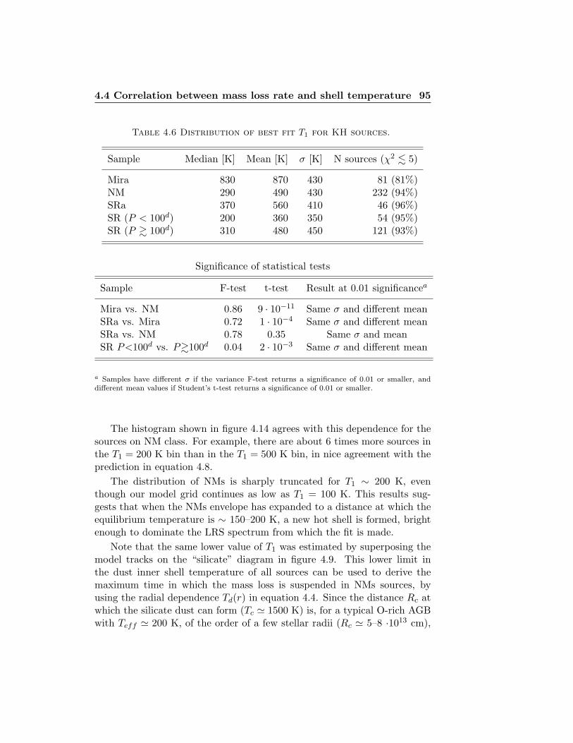
Table 4.6 Distribution of best fit T1 for KH sources.

Sample Median [K] Mean [K] σ [K] N sources (χ2 . 5)

Mira 830 870 430 81 (81%)NM 290 490 430 232 (94%)SRa 370 560 410 46 (96%)SR (P < 100d) 200 360 350 54 (95%)SR (P & 100d) 310 480 450 121 (93%)



Mira vs. NM 0.86 9 · 10−11 Same σ and different meanSRa vs. Mira 0.72 1 · 10−4 Same σ and different meanSRa vs. NM 0.78 0.35 Same σ and meanSR P<100d vs. P&100d 0.04 2 · 10−3 Same σ and different mean


The histogram shown in figure 4.14 agrees with this dependence for thesources on NM class. For example, there are about 6 times more sources inthe T1 = 200 K bin than in the T1 = 500 K bin, in nice agreement with theprediction in equation 4.8.

The distribution of NMs is sharply truncated for T1 ∼ 200 K, eventhough our model grid continues as low as T1 = 100 K. This results sug-gests that when the NMs envelope has expanded to a distance at which theequilibrium temperature is ∼ 150–200 K, a new hot shell is formed, brightenough to dominate the LRS spectrum from which the fit is made.

Note that the same lower value of T1 was estimated by superposing themodel tracks on the “silicate” diagram in figure 4.9. This lower limit inthe dust inner shell temperature of all sources can be used to derive themaximum time in which the mass loss is suspended in NMs sources, byusing the radial dependence Td(r) in equation 4.4. Since the distance Rc atwhich the silicate dust can form (Tc ' 1500 K) is, for a typical O-rich AGBwith Teff ' 200 K, of the order of a few stellar radii (Rc ' 5–8 ·1013 cm),


one can write:

R1 ∼ 5− 8 · 1013 cm(

1500KT1

)2

(4.9)

being Rs ∼ 1 A.U. the average stellar radius in the AGB phase. A dust shellwith T1 ' 200 K should thus be located at a distance R1 ' 0.9–1.7 ·1016 cm.Assuming an expansion speed about 15 km/s, the required time to produce adetached shell at such distance is then 100–200 yr. Note that the estimatedtime scale is too long to compare with the Mira/SR pulsational period, andtoo short with respect to the interpulse time in the TP-AGB phase. It ishowever consistent with the timescales observed by Hashimoto et al. (1998);Sahai et al. (1998); Mauron & Huggins (1999), and by the independentestimate made in section 3.3.5 (see also Marengo et al., 1999).

The timescale of the high mass loss duration phase, in which the dustenvelopes are created, can also be estimated by counting the fraction ofNMs in the high temperature bins (e.g. T1 & 500 K). Since this fraction isabout 30%, the phase of intense dust production should last no more than30–60 yr, assuming 100-200 yr as the total period of the mass loss cycle.

Miras, on the contrary, show a flat distribution, truncated at a muchhigher T1. This is an evidence that Mira sources have a higher dust produc-tion efficiency, which prevents the complete detachement of their circum-stellar envelopes, and their cooling to very low temperatures.

The parameters of the T1 distribution for the various subsamples arewritten in table 4.6. They confirm the separation between Miras and NMsand the homogeneity of SRa with the global NM class. The two subclasses ofSRs with long and short pulsational period, however, does show a differentmean value, with short period SRs having colder dust than the long periodones. This difference, however, has low statistical significance, and can bedue to statistical fluctuations in our sample.

4.4.3 Distribution of mass loss rates

From the best fit parameters of each source, it is possible to estimate themass loss rate. By integrating the differential optical depth along the pathas in equation 4.3, with a “steady mass loss” radial density profile nd(r) 'nd(R1) · (R1/r)2, one obtains:

τV ' πa2 ·QV · nd(R1)R1 (4.10)


Fig. 4.15.— Distribution of best fit mass loss rate M for Miras (dashed line), NMs(solid line) and SRa (dotted line).

where a is the dust average grain radius and QV the opacity at optical wave-length. For a spherically symmetric dust envelope with constant expansionvelocity ve, the mass loss rate is:

M ' 4πr2 · ve · µdρr (4.11)

where µd is the dust to gas mass loss ratio and ρr ' 4/3πa3 · ρd · nd(r) themass density distribution of the circumstellar shell, made of individual dustgrains having mass density ρd. Combining equation 4.10 with equation 4.11one has:

M ' 16πa

3· µdρd · ve

QV· τV ·R1 (4.12)

For the sources in our KH sample, one can assume ρd ' 3.9 g cm−3 asin terrestrial silicates, a ' 0.1 µm, QV ' 1, ve ' 15 km/s and µd ' 100.Using equation 4.9, one finally obtains the following approximation for themass loss rates, as a function of the two fitting parameters τV and T1 alone:


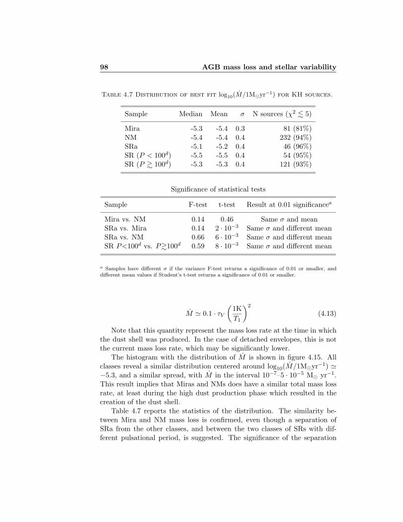
Table 4.7 Distribution of best fit log10(M/1M¯yr−1) for KH sources.

Sample Median Mean σ N sources (χ2 . 5)

Mira -5.3 -5.4 0.3 81 (81%)NM -5.4 -5.4 0.4 232 (94%)SRa -5.1 -5.2 0.4 46 (96%)SR (P < 100d) -5.5 -5.5 0.4 54 (95%)SR (P & 100d) -5.3 -5.3 0.4 121 (93%)



Mira vs. NM 0.14 0.46 Same σ and meanSRa vs. Mira 0.14 2 · 10−3 Same σ and different meanSRa vs. NM 0.66 6 · 10−3 Same σ and different meanSR P<100d vs. P&100d 0.59 8 · 10−3 Same σ and different mean


M ' 0.1 · τV

(1KT1

)2

(4.13)

Note that this quantity represent the mass loss rate at the time in whichthe dust shell was produced. In the case of detached envelopes, this is notthe current mass loss rate, which may be significantly lower.

The histogram with the distribution of M is shown in figure 4.15. Allclasses reveal a similar distribution centered around log10(M/1M¯yr−1) '−5.3, and a similar spread, with M in the interval 10−7–5 · 10−5 M¯ yr−1.This result implies that Miras and NMs does have a similar total mass lossrate, at least during the high dust production phase which resulted in thecreation of the dust shell.

Table 4.7 reports the statistics of the distribution. The similarity be-tween Mira and NM mass loss is confirmed, even though a separation ofSRa from the other classes, and between the two classes of SRs with dif-ferent pulsational period, is suggested. The significance of the separation

4.5 Conclusions 99

is however very low, and can be attributed to statistical fluctuations in oursample, or to the high uncertainties in the quantities assumed to deriveequation 4.13 (and in particular the dust to gas mass loss ratio and theaverage grain size).

4.5 Conclusions

In this analysis we have investigated the connections between mass lossand variability for a sample of AGB LPV of Mira, SR and Irregular type,from the point of view of the mid-IR emission of their dusty circumstellarenvelopes.

We found the continuum excess color in the 12.5 and 18.0 µm bandsable to differentiate between sources of Mira and NM type. NMs showed ahigher [12.5]-[18.0] color, which we interpreted as an indication of missinghot dust in the circumstellar envelope of these sources.

We then compared the position of 10 µm silicate feature in the LRSspectrum of Mira and NM sources, confirming the shift of ∼ 0.2 µm alreadyfound by other authors. Even though this result may be taken as an evidencefor mineralogical variability in the composition of oxidic dust in the two classof sources, we have pointed out how radiative transfer may mimic the sameeffect. If this is the case, the shift observed in the LRS of NMs can beanother consequence of colder dust in their envelopes.

We then applied radiative transfer modeling to all sources in the sample,in order to derive their optical depth and temperature at the inner shellboundary by fitting their individual Low Resolution Spectra. Again wefound a statistically significant difference between the temperature of NMand Mira circumstellar envelopes.

About 70% of all NMs in our sample show a τV vs. T1 relation that is ap-propriate for detached envelopes, expanding freely at the AGB wind speed.For these sources, the inner boundary shell temperature is much lower thanthe dust condensation one, but never less than 150–200 K. This minimumtemperature can be interpreted as a maximum limit of 100-200 yr in theperiod of time in which the envelopes are allowed to detach, before beingreplaced by newly formed hot structures. The remaining part of the NMsare instead characterized by much hotter envelopes with an estimated T1 inthe dust condensation and growth range (Tc ∼ 600–1400 K), in which theenvelope is not complete detached. The frequency of these sources (∼30%)suggests that the duration of the high mass loss phase in NMs is of the or-der of 30–60 yr. The two regimes are linked by an intermediate domain, in


which T1 ∼ 500 K, where the optical depth of the envelope suddenly dropsby one order of magnitude.

The proportion between “hot” and “cold” envelopes in the Mira classis reversed with respect to NMs, with 70% of Miras having T1 & 500 K.This dependence shows that fully detached shells are probably not commonin the Mira class. The 1 magnitude drop in the total optical depth of theenvelopes around T1 ∼ 500 K, is confirmed for this class of sources, andcan thus be related to some basic property of the silicate dust condensationprocesses.

We did not find any significant difference in the total mass loss rates ofMiras and NMs, even though the frequent occurrence of detached shells inNMs suggests the existence of intermittent phases in which the dust pro-duction is suspended for these sources.

All our statistical tests confirm that our subsample of SRa is coherentwith the full sample of NMs (SRa, SRb and Irregulars) in our selection ofKH sources. We also did not find any significant difference between SRswith long and short period pulsations, that can be associated with differentphases in the AGB evolution.

As suggested by Ivezic & Knapp (1998), the absence of hot dust in NMscan be interpreted as a recent decrease (∼ 102 yr) in their mass loss rates.In the same paper were also found evidences for mass loss to resume onsimilar timescales, implying that AGB stars may oscillate between the Miraand NM phase, as proposed by Kerschbaum & Hron (1996). This idea ishowever discarded in a recent paper by Lebtzer & Hron (1999), in which theabundance of 99Tc in a large sample of SRs was compared with the analogousquantity in Miras. Since the Tc abundance is characterized by a quickincrease during the first thermal pulse, after which it stays basically constant(Busso et al., 1992), a similar fraction of Tc-rich stars should be found inthe Mira and SR samples. However, this is not the case, making it unlikelythat TP-AGB variables oscillates between the two classes of pulsators.

Our analysis confirms the occurrence of shell detachment in NM vari-ables, but suggests a different explanation. The discordant behavior of massloss between Miras and NMs may be due to a different efficiency of oxidicdust formation in the two cases. This may be related to the characteristicpulsational mode of the two classes of variables.

Many separate evidences points toward the idea that SR variables pul-sate as a combination of several overtones, while Miras are high amplitudepulsators (Wood et al.,, 1999), even though this subject is quite controver-sial (see e.g.Feast 1999, proceedings of the same I.A.U. conference). If thisis the case, it is likely for Mira variables to have a greater efficiency in lev-

4.5 Conclusions 101

itating their extended atmosphere to regions where the dust condensationis possible (see discussion of Icke et al. 1992 models in Sahai et al. 1998).As a consequence, Miras extended atmospheres would be able to support acontinuous mass loss rate by providing enough molecules in the right den-sity and temperature range for dust condensation and growth. NMs, on thecontrary, would need several pulsation cycles to reach the critical densityfor dust formation to start. The increasing opacity resulting from dust nu-cleation would then trigger an outburst of dust production, lasting until thedust building elements are depleted, after which the envelope detaches. Inthis case, the active phase in which the mass loss is active in NM variablesshould be of the order of 30%, of the total cycle, according to the ratio ofNMs which do not show a detached shell.

This dynamical mechanism has been partially reproduced in time depen-dent wind models (Winters, 1998), but the observed timescales (5–10 yr) arestill too short to explain the observed shells. Based on our analysis, we can-not favor any particular mechanism for the occurrence of interrupted massloss in NM sources. We feel, however, that dynamical models trying to re-produce the mass loss of AGB pulsators should take into account this linkbetween the efficiency of dust production and the pulsational type, and thepresence of detached dust shells found by analyzing the relations betweenτV and T1 in the two classes of sources.

agb mass loss and stellar variability

Documents