afit/gor/ens/94m- 15 · today's air force. his contributions to this research and my career...

AD-A278 551 4(1

AN RSM STUDY OF THE EFFECTS OFSIMULATION WORK AND METAMODELSPECIFICATION ON THE STATISTICAL

QUALITY OF METAMODEL ESTIMATES

THESIS

Mfichael Kent Taylor, Captain, USAF -

AFIT/GOPJENSI94M- 15 D I

DEPARTMENT OF THE AIR FORCEAliR UNIVERSITY

AIR FORCE INSTITUTE OF TECHNOLOGYD=~C WtALMp 121SPECTED 3

Wright-Patterson Air Force Base, Ohio

AFIT/GOR/ENS/94M- 15

Acceslon For

NTIS CRA&IDTIC TABU( .announced 0Justification

By ................Dist. ibution I

Availability Codes

Avail and / orDist Special



THESIS

Michael Kent Taylor, Captain, USAF


S"Al

-J

Approved for public release; distribution unhned.

94-12283III~ ~ ~ ~~" 1141 I III~

The views expressed in this thesis are those of the author and do not reflect theofficial policy or position of the Department of Defense or the U.S. Government.


An RSM Study of the Effects of Simulation Work and MetamodelSpecification on the Statistical Quality of Metamodel Estimates

Thesis

Presented to the Faculty of the Graduate School of Engineering

of the Air Force Institute of Technology

Air University

In Partial Fulfillment of the

Requirements for the Degree of

Master of Science in Operations Research

Michael Kent Taylor, Captain, USAF

March 1994

Approved for public release; distribution unlimited

THESIS APPROVAL

STUDENT: Capt Michael Kent Taylor CLASS: GOR-94M

THESIS TITLE: An RSM Study of the Effects of Simulation Work and MetamodelSpecification on the Statistical Quality of Metamodel Estimates

DEFENSE DATE: 01 March 94

COMMITTEE:

NAME/DEPARTMENT SIGNATURE

Advisor: Lt Col Paul F. AuclairAssistant Professor of Operations ResearchDepartment of Operational Sciences, AFIT/ENS

Reader: Dr Edward F. Mykytka (,a~o /

Associate Professor of Operations ResearchDepartment of Operational Sciences, AFIT/ENS

Acknowledgments

This research endeavor would not have been possible without the help of others.

My research committee, especially Lt Col Paul Auclair, provided guidance so that I was

not "all mach and no vector." Lt Col Auclair continues to distinguish himself as a

professional Air Force officer and as an OR practitioner, solving the problems that face

today's Air Force. His contributions to this research and my career are invaluable. My

reader, Dr Ed Mykytka provided valuable "end-game" assistance, comments, and

readership to round-out my thesis. Others at AFIT who assisted me are numerous --

special thanks goes to my two favorite librarians, Pam and Cindy. There are also many

before AFIT who have contributed to my development academically and as a research

novice -- most notably, Gloria Kearin, Neal Urquhart, Dr Charles Katholi, and Dr James

Crenshaw. In addition, there are those outside of AFIT who have contributed to my

development as an Air Force officer. P.J., Rocket Man, J.P., Sprengs, Gunx, Goose, and

Merle are only a few that often cause me to reflect on "What have I done for Blue-4

today?" Also deserving honorable mention are Sam Adams, Riley B. King, John Lee, and

Bobby Cray -- they have certainly done their share of inspiration.

I would be remiss if my parents were not mentioned here as contributing to my

development as a person. Even more so, I must mention Vicky Erlanger. Her inspiration

will continue beyond this thesis. No matter what the future may hold, she is truly and

completely sui generis. I am the lucky one.

Table of Contents

Acknowledgments ii

List of Figures v

List of Tables vi

Abstract viii

I. Introduction1.0. Background 1-11.1. Problem Statement 1-31.2. Objective 1-41.3. Methodology Overview 1-41.4. Summary 1-5

II. Background2.0. Introduction 2-12.1. Simulation 2-12.2. Response Surface Methodology

2.2.0. Introduction 2-32.2.1. Least Squares Regression 2-52.2.2. Experimental Design 2-5

2.3. Metamodels 2-72.4 M/M/k Queues 2-102.5. Summary 2-10

III. Methodology3.0. Introduction 3-13.1. Queuing Simulations

3.1.0. Introduction 3-13.1.1. Queuing Configurations 3-13.1.2. Simulation Work Cases 3-23.1.3. Summary 3-4

3.2. Analytical Solutions 3-43.3. Simulation Estimates 3-63.4. Metamodel Estimates 3-73.5. Residual Analysis 3-133.6. Summary 3-15

111oi

IV. Results and Analysis4.0. Introduction 4-14.1. Graphic Analysis

4.1.0. Introduction 4-I4. 1.1. Mean of Residuals 4-14.1.2. Standard Error of Residuals 4-34.1.3. Range of Residuals 4-44.1.4. Summary of Graphic Analysis 4-6

4.2. Single-Factor ANOVA4.2.0. Introduction 4-64.2.1. Null Hypotheses for F-tests 4-74.2.2. F-test Results 4-74.2.3. Summary of ANOVA and F-tests 4-7

4.3. Metamodel Comparison 4-84.4. Summary 4-9

V. Conclusions and Recommendations5.0. Introduction 5-15.1. Conclusions 5-15.2. Recommendations

5.2.0. Introduction 5-25.2.1. Queuing Networks 5-25.2.2. Queuing Statistics 5-25.2.3. Different System 5-35.2.4. Fractionation and Metamodels 5-3

5.3. Summary 5-3

Appendix A: Simulation Overview A-I

Appendix B: Simulation Residual Data B-1

Appendix C: Full Metamodel Residual Data C-1

Appendix D: Fractional Metamodel Residual Data D-1

Appendix E: Simulation, Full, and Fractional Metamodel ANOVA Data E-i

Appendix F: Metamodel Comparison Data F-1

Bibliography Bib-I

Vita V-i

iv

List of Figures

Figure Page

2-1. Ways to Study a System 2-3

4-1. Mean of Residuals for Simulation and All Metamodelsvs. Simulation Work 4-2

4-2. Standard Error of Residuals for Simulation and All Metamodelsvs. Simulation Work 4-3

4-3. Range of Residuals for Simulation and All Metamodels vs. Simulation Work 4-5

4-4.. R-Squared Values, Fuli and Fractional Metamodels 4-9

A-I. Example SLAMSYSTEM Model, Configuration 1, Case A A-1

V

List of Tables

Table Page

2-1. Full Factorial Design, 3 Factors at 2 Levels 2-6

2-2. Fractional Factorial Design, 3 Factors at 2 Levels 2-7

2-3. Metamodel Formulation 2-9

3-1. Queuing Configurations 3-2

3-2. Original Simulation Work Cases 3-2

3-3. Final Simulation Work Cases 3-4

3-4. Analytic Solutions: Average Queue Length 3-6

3-5. Simulation Results: Example Data, Case A 3-7

3-6. Fractional Factorial Design for M/M/k Queuing Configurations 3-8

3-7. Predictive Metamodel Forms 3-9

3-8. Example SAS Output: Full Linear Metamodel, Case A 3-10

3-9. Example SAS Output: Full Logarithmic Metamodel, Case A 3-10

3-10a. Example Data: Full Linear-Neg Metamodel Residual Statistics 3-12

3-10b. Example Data: Full Linear-Zero Metamodel Residual Statistics 3-12

3-10c. Example Data: Full Logarithmic Metamodel Residual Statistics 3-13

3-11. Residual Analysis: Full Logarithmic Metamodel, Case A 3-14

3-12. Residual Analysis: Mean of Residuals from Simulation and All Metamodels 3-15

4-1. F-test Results 4-7

B-I. Summary of Simulation Residual Data B-1

vi

C-I. Summary of Fu'll Linear-Neg Metamodel Residual Statistics C-I

C-2. Summar, J Full Linear-Zero Metamodel Residual Statistics C-I

C-3. Summary of Full Logarithmic Metamodel Residual Statistics C-I

D-1. Summary of Fractional Linear-Neg Metamodel Residual Statistics D-I

D-2 Summary of Fractional Linear-Zero Metamodel Residual Statistics D-1

D-3. Summary of Fractional Logarithmic Metamodel Residual Statistics D-I

E-I. Mean of Residuals for Simulation and All Metamodels E-I

E-2. Standard Error of Residuals for Simulation and All Metamodels E-I

E-3. Range of Residuals for Simulation and All Metamodels E-2

F-I. Summary of Full Linear Metamodels F-I

F-2. Summary of Full Logarithmic Metamodels F-2

F-3. Summary of Fractional Linear Metamodels F-3

F-4. Summary of Fractional Logarithmic Metamodels F-4

vii

Abstract

Intuitively, simulation estimates can be improved by increasing the number of

simulation replications, run lengths, or both. Estimates from metamodels of simulation

data can be improved by proper model selection, or model "specification." Although the

individual effects of doing "more" simulation work and using a "smarter" metamodel were

well known, the combined effects of fitting metamodels to simulation data with different

amounts of work was unknown.

This research investigated the influence of the amount of simulation work and

metamodel specification on the statistical quality of the estimates obtained from

metamodels of the simulation data. A 9 x 2 x 2 experiment consisting of 9 cases of

simulation work, 2 levels of metamodel specification, and 2 levels of design fractionation

were designed for 8 different configurations of M/M/k queues. The only observed statistic

for this experiment was the average queue length. Simulation estimates for each

configuration's average queue length were calculated directly from the simulation data. In

addition, metamodel estimates for each configuration's average queue length were

calculated using the metamodels fit to each case of simulation data.

Residuals were calculated for each of these respective estimates as the difference

between the analytic solution for average queue length and the given estimate. Graphic

analysis and Single-Factor ANOVA were performed on the residual data to determine if

the amount of simulation work or metamodel specification affected the statistical quality

of the estimates. This research showed conclusively that the amount of simulation work

had no significant effect and that the metamodel specificaion had a significant effect on

the statistical quality of the estimates found using the metamodels.

viii



1. Introduction

1.0. BackgroundComputer simulation is

the process of designing a model of a real system and conducting experiments withthis model for the purpose of either understanding the behavior of the systemand/or evaluating various strategies for the operation of the system [Shannon,1992:65].

Shannon also asserts that simulation modeling is "an experimental and applied

methodology" which seeks, among other things, "to predict ... the effects that will be

produced by changes in the system or in its method of operation." The ability of computer

simulations to "predict" system performance is often limited by several factors, most

notably, restrictions on computer and analysis resources. Given the opportunity, most

simulation practitioners would prefer "more" simulation rather than "less" to estimate the

performance of the system under study. Such preference for "more" simulation is

statistically well-founded and may be achieved primarily in either of two ways. First, the

number of simulation replications can be increased. Second, the length of each simulation

can be increased [Goldsman, 1992:98-99]. Thus, preference is given to simulations with

more replications, run length, or both. In fight of the more realistic limitations and

restrictions noted above, simulation practitioners are faced with trade-offs between

1-1

replications and run length. The primary implication of these trade-offs is that the

precision of the estimated performance measure is a function of the simulation length and

number of replications. Several sources address these trade-offs and their implications

[Law and Kelton, 1991:Ch 9; Whitt, 1991:645-665]. For the this research, the amount of

simulation "Work" was defined as the product of the number simulation replications and

the simulation run length.

Just as computer simulations can be used to estimate the performance of real

systems, metamodels can be used as surrogates of the computer simulation in order to

estimate the performance of the real system. The term "metamodel" was originated by

Kleijnen. He defined it as a regression model of simulation input and output data

[Kleijnen, 1987:Ch 11]. Sargent furthers the definition -- "the objective of a metamodel is

to effectively relate the output data of a simulation model to the model's input to aid in the

purpose for which the simulation model was developed' [Sargent, 1992:888].

Accordingly, the combinations of simulation input and output data may be regressed into a

functional form that is, in effect, a model of the model. The metamodel can then be

evaluated at points within the experimental design matrix of the input parameters, in order

to estimate the desired performance characteristic without actually reaccomplishing the

simulation with the new set of input parameters. Since simulations are costly to run and

analyze, metamodel estimates can be used as a surrogate for the simulation at an obvious

cost savings in terms of both computer and analysis time. For example, rather than run

and analyze a full simulation over an entire range of input parameters, a second-order

polynomial metamodel of the simulation data with few variables can be evaluated for a

single set of input parameters in a matter of seconds [Yielding, 1991:78]. More complex

metamodels "can be run iteratively many times for repeated 'what if evaluation for multi-

objective systems or for design optimization" [Barton, 1992:289].

1-2

The computational ease of using metamodels is done at the expense of precision in

the estimated performance characteristic since the least squares metamodel is built by

providing the "best" fit for all the data -- some points will be "better" fit than others

[Neter, Wasserman, and Kutner, 1990:47-49]. Thus, the ability of the metamodel to

provide precise estimates of the simulation performance is largely dependent on the model

form or "specification" [Friedman, 1985:145]. Metamodel specification is a function of

the number and type of variables used in the least squares regression equation to produce

an acceptable level of predictive validity. Predictive validity is defined here as the ability

of a metamodel to produce valid estimates of the computer simulation -- and therefore of

the performance of the real system. Just as with regression models, the fit and predictive

validity of a metamodel can be improved primarily by either transforming the existing

variables in the model or by adding new terms to the model [Kleijnen, 1987:Ch 14].

Variable transformations may be applied to either the input or the response data, or both.

Common transformations include the logarithmic, square root, and reciprocal

transformations [Neter, Wasserman, and Kutner, 1990:142-151 ]. Adding terms to the

metamodel may be useful when trying to fit data with curvature or interaction effects

[Neter, Wasserman, and Kutner, 1990:248]. However, these methods for improving the

predictive validity of the metamodel should not be done to the point of overly specifying a

metamodel with insignificant terms that, when added, only contribute a relatively small

improvement to the metamodel's predictive validity. Therefore, the "best" metamodels are

parsimonious; they provide acceptable estimates of the computer simulation while

containing as few terms as possible.

1.1. Problem Statement

Much research has been devoted to studying the topics of simulation work and

metamodel specification. It has been shown that increasing the amount of simulation work

1-3

increases the statistical quality of the estimated response. In addition, much research has

been devoted to improving metamodel estimates by selecting a properly specified

metamodel. Absent from this research, however, is an investigation of how different

amounts of simulation work affect the statistical quality of estimates from the resulting

metamodels.

1.2. Objective

The purpose of this research was to determine how the amount -of simulation work

and the specification of the metamodel affect the statistical quality of the estimates

obtained from the resulting metamodels of the simulation data.

1.3. Methodology Overview

In the pursuit of this objective and for the sake of simplicity, M/M/k queues were

simulated over a range of system parameters and utilization rates (8 total configurations)

and with various combinations of simulation replications and run lengths (9 total cases).

The only observed output from each simulation was the average queue length.

From these simulations, the mean of the average queue lengths was calculated for

each queuing configuration within each case of simulation work. This mean was the

"simulation estimate" used as a baseline for comparing the estimates obtained from the

resulting metamodels. To calculate the estimated average queue length from the

metamodels, a logarithmic and a linear metamodel were fit to the simulation data using

least squares regression. The metamodels were fit using the arrival rate, service rate, and

number of servers as inputs. The response variable for the metamodels was the average

queue length estimated for each case of simulation work.

1-4

Analytical solutions were calculated for each configuration. These analytic results

were treated as the "known" solution for each queuing configuration and were compared

to the estimated average queue length obtained from simulation and the metamodels. In

this research, the "residual" was defined as the difference between the analytic solution and

the estimated average queue length for each of the eight queuing configurations.

Residuals were used to investigate the effect of simulation work and metamodel

specification on the statistical quality of the metamodel estimates. Specifically, the mean,

standard error, and range of the residuals were calculated for each case of simulation

work.

The residual statistics from the respective estimators (i.e., simulation and

metamodels) were analyzed graphically and by Single-Factor Analysis of Variance

(ANOVA). In particular, ANOVA was performed on the data for each residual statistic,

using appropriate F-tests, to determine if either the amount of simulation work or the

metamodel specification affected the residual statistics.

1.4. Summary

Simulation is used to study real systems as part of an overall modeling process that

seeks to determine the relationship between the inputs and outputs of a given system and

to estimate the performance of the system. Similarly, metamodels are part of the modeling

process used to study the real system by modeling the simulation data.

The implications of increasing simulation work are well known -- quite simply,

"more is better." The implications of metamodel specification are also well known --

selecting a better-specified metamodel, which includes the type and number of input

factors, improves the metamodel estimates of the computer simulation. However, the

effect of simulation work and metamodel specification on the statistical quality of the

1-5

resulting metamodels had not been well established in the literature available at the onset

of this study.

The purpose of this research was to determine the effects of simulation work and

metamodel specification on the statistical quality of the estimates obtained from

metamodels of the simulation data. These effects were investigated by:

"Systematically designing and simulating M/M/k queues with different levels of

simulation work,

" Fitting the simulation data with metamodels of differing specification, and

" Comparing the statistical quality of the residuals from the resulting metamodelestimates.

1-6

2. Background

2.0. IntroductionAs stated in Chapter 1, the purpose of this research was to determine how the

amount of simulation work and the metamodel specification affect the statistical quality of

the estimates obtained from the resulting metamodels of the simulation data. The

experimental approach implemented to attain this research objective relied heavily on:

Computer Simulation, Response Surface Methodology, Metamodels, and M/M/k queues.

Brief discussions for each subject are presented here -- interested readers are referred to

respective sources listed in each section for a more detailed and lengthy discussion.

2.1. SimulationComputer simulation is the process whereby a computer is used to evaluate a

mathematical model of a system. In this context, a system is any process composed (f

input factors and one or more output responses. Virtually any system may be simulated

via a computer. Typical applications include simulations of inventory systems, traffic

analysis, tanker refinery operations, and job-shop scheduling [Pritsker, 1986]. Quite

often, managers and decision makers must determine whether to invest in new equipment

or to modify existing procedures in order to best use available resources in pursuit of their

objectives. Consider, for example, a manufacturing situation with an objective of

maximizing its production. Faced with a decision to add an entire shift of workers or to

replace aging equipment with newer, more capable equipment that doesn't require

additional workers, analysts and decision makers would like a cost-effective way to

analyze the effects and trade-offs of either course of action. These alternatives could be

evaluated in either of two ways [Law and Kelton, 1991:3-7]. First, the actual system

2-1

could be altered. In this case, the two policy alternatives could be evaluated by hiring and

training a new shift of workers and observing their productivity over a given period of

time. Later, the new shift of workers could be eliminated in order to test the efficacy of

the equipment modernization option. At the end of the test, the data for the two options

could be compared and the superior alternative selected. However, this process has

obvious drawbacks. In the first case of hiring and then laying-off a new shift of workers,

the cost of training the employees as well as paying their wages during the lay-off must be

considered. There is also a cost in terms of public opinion as the company runs the risk of

being viewed as disingenuous with regard to their commitment to the local community and

workforce. On the other hand, the investment in equipment must not be taken lightly. If

the new shift option proved to be more advantageous, the company could be saddled with

used equipment which may not have a market for resale. For these and other reasons,

experimenting with the actual system might be impractical. The second way of

determining these trade-offs would be to experiment with a model of the system.

Such experimentation is generally conducted with either physical or mathematical

models [Law and Kelton, 1991:3-7]. The above manufacturing example is a case where a

physical model is probably not practical since replicating a manufacturing plant would be a

very difficult and costly process. There are, however, systems that avail themselves to

physical models. For example, aeronautical engineers use scaled-down aircraft models to

study airflow patterns in wind tunnels.

As an alternative to physical models, mathematical models use quantitative and

logical relationships to characterize the system. For relatively simple mathematical

models, analytical solutions can be calculated in order to characterize the performance of

the system. If, in the manufacturing example, production rates of either alternative could

be computed directly as a function of the number of employees and the number of

machines in use, it would be a straight-forward task to determine which alternative yielded

2-2

the higher production rate. It is more often the case, however, that the complex logical

and quantitative relationships that characterize the system preclude a direct solution to the

model. For highly complex or intractable models, computer simulation provides a means

to exercise and evaluate a given mathematical model over its full domain. Figure 2-1,

modified from Law and Kelton, summarizes this approach to modeling. The shaded

portion of the diagram highlights the focus of this research.

Figure 2-1. Ways to Study a System [Law and Kelton, 1989:4]

Experiment withSa m odel of Physical M odel

the system

Experiment with Mathematical Analyticalthe actual system Model Solution

ComputerSimulation

2.2. Response Surface Methodology

2.2.0. Introduction. Whereas computer simulations can be used to model a given

system and metamodels can be used to model the given computer simulation of the

system, Response Surface Methodology (RSM) is an efficient and systematic approach to

developing either of these models of system performance. RSM

2-3

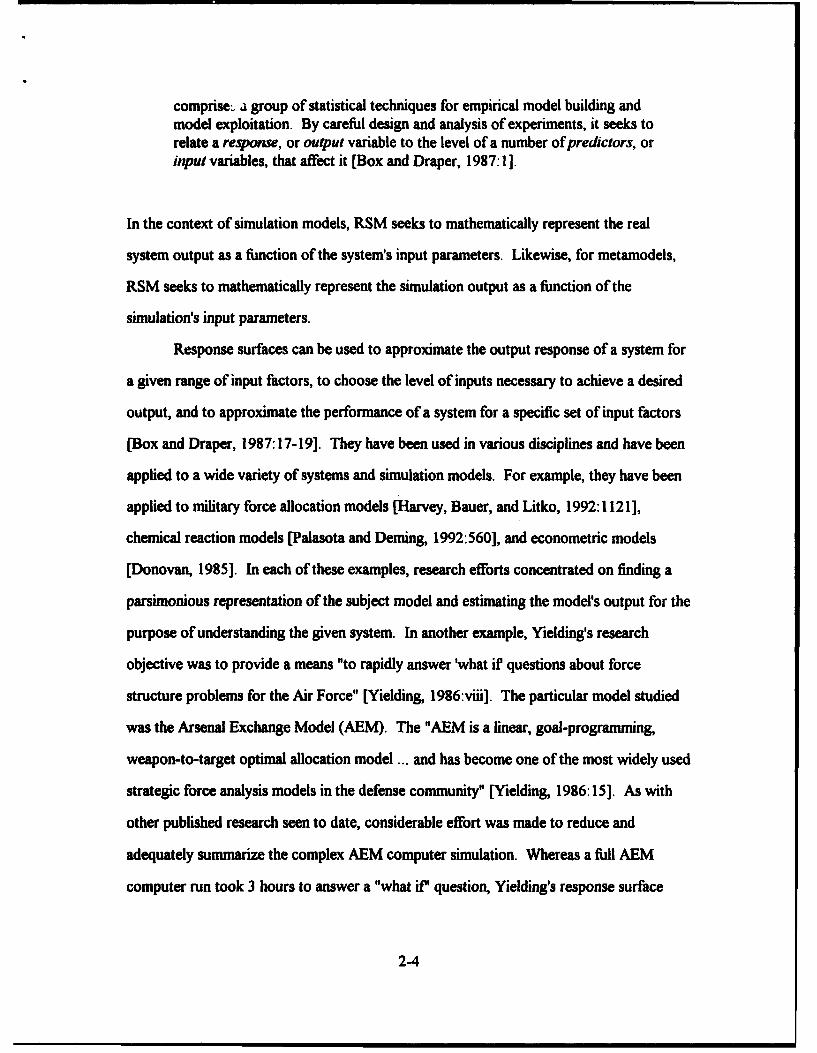
comprisez, a group of statistical techniques for empirical model building andmodel exploitation. By careful design and analysis of experiments, it seeks torelate a response, or output variable to the level of a number of predictors, orinput variables, that affect it [Box and Draper, 1987:1].

In the context of simulation models, RSM seeks to mathematically represent the real

system output as a function of the system's input parameters. Likewise, for metamodels,

RSM seeks to mathematically represent the simulation output as a function of the

simulation's input parameters.

Response surfaces can be used to approximate the output response of a system for

a given range of input factors, to choose the level of inputs necessary to achieve a desired

output, and to approximate the performance of a system for a specific set of input factors

[Box and Draper, 1987:17-19]. They have been used in various disciplines and have been

applied to a wide variety of systems and simulation models. For example, they have been

applied to military force allocation models [Harvey, Bauer, and Litko, 1992:1121],

chemical reaction models [Palasota and Deming, 1992:560], and econometric models

[Donovan, 1985]. In each of these examples, research efforts concentrated on finding a

parsimonious representation of the subject model and estimating the model's output for the

purpose of understanding the given system. In another example, Yielding's research

objective was to provide a means "to rapidly answer 'what if questions about force

structure problems for the Air Force" [Yielding, 1986:viii]. The particular model studied

was the Arsenal Exchange Model (AEM). The "AEM is a linear, goal-programming,

weapon-to-target optimal allocation model ... and has become one of the most widely used

strategic force analysis models in the defense community" [Yielding, 1986:15]. As with

other published research seen to date, considerable effort was made to reduce and

adequately summarize the complex AEM computer simulation. Whereas a full AEM

computer run took 3 hours to answer a "what if" question, Yielding's response surface

2-4

model generates valid answers in a matter seconds [Yielding, 1986:78]. Results such as

these typify the benefits of using RSM on large, complex models.

Two specific RSM "techniques" are used in this research and are discussed here --

least squares regression and experimental design. These and other techniques, such as

steepest ascent methods and multi-response systems, are discussed in detail in three

notable texts, Applied Regression Analysis, [Draper and Smith, 1981 ], Empirical Model-

Building and Response Surfaces, [Box and Draper, 1987], and Response Surfaces [Khuri

and Cornell, 1987].

2.2.1. Least Squares Regression. Simply stated, least squares regression seeks to

"fit" the given output data from the simulation with a function whose form is based upon

the inputs of the simulation. The regression function can be used to predict the output

response for a set of given inputs which may not have been in the original design matrix.

In addition, the regression function can be used to determine the relative significance of

input factors in the design region as determined via statistical methods [Neter, Waterman,

and Whitmore, 1988:Ch 20]. Effective regression modeling also facilitates the

development of parsimonious models that further the overall goal of simulation and

metamodeling - the adequate representation of a complex system or computer simulation

of the system in a simpler, more efficient way.

2.2.2. Experimental Design. As noted previously, RSM is used to study the

relationship between outputs and input factors of a system. Experimental Design is an

RSM technique whereby "purposeful changes are made to the input factors of a process or

system so that we may observe and identify the reasons for changes in the output

response" [Montgomery, 1991:1].

The simplest way to systematically vary the input of k factors is to set each factor

to two levels. The set of all possible combinations of factors set at their respective levels

is termed a full factorial design. For example, with k = 3 input factors set at two levels,

2-5

there are 2-' =8 configurations of input factors for use in experimentation with the system

or simulation model. Table 2-1 shows the 8 configuration resulting from three inputs (A,

B, and C) set to two levels (denoted with "+" and "- signs to indicate the two levels,

respectively).

Configuration A B C1 + + +

2 + +

3 + +

4 + -5 + +

6 +7 +

8 1 "

Table 2-1. Full Factorial Design, 3 Factors at 2 Levels

Factorial designs allow multiple comparisons to be made to facilitate model creation,

provide highly efficient estimates of model parameters, and usually involve simple

calculations [Box and Draper, 1987:106]. Box and Draper note that two level designs are

especially useful in the exploratory stages of an investigation when little is known about

the system and the model structure is relatively unknown. Other designs useful in

experimenting with other specific model forms, are discussed in the texts noted above in

Section 2.2.0.

Since the number of input combinations for a two level factorial design increases

by a factor of 2 for each increase in the number of input factors, the set of all input

combinations grows rapidly as the number of input factors is increased. When resources

are limited and all input combinations cannot be evaluated, it is possible to study the

system by carefully choosing a fraction of the fili set of input factor combinations for

2-6

evaluation. Designs such as these are fractional factorial designs Detailed methods for

fraction selection, confounding, and alias structures are presented in the previously noted

Box and Draper text, Chapter 5. As an example of a "half-fraction," consider the previous

three factor, two level example as the full factorial design to be used for experimentation.

The two half-fractions found by using the three factor interaction term ABC as the block

generator are shown below in Table 2-2. Though fractional designs and experiments are

less costly to perform and analyze, they provide estimates for only selected factors and

interactions. Hence, consideration should be given so that all relevant factors can be

estimated when using fractionated designs.

Configuration A B C ABC FractionI + + + +2 + + - - 23 + - + - 24 + - + 15 - + + - 26 - + - +7 - - + +

8 .... 2Table 2-2. Fractional Factorial Design, 3 Factors at 2 Levels

2.3. Metamodels

As noted in Chapter 1, the term "metamodel" is used to denote a model of a model

[Kleijnen, 1987:147]. Sargent asserts that metamodels are used to "relate the output data

of a simulation model to the model's input" [Sargent, 1991:888]. Thus, in the context of

RSM, a metamodel is a response surface of simulation data. Thus, all of the RSM

techniques used to "build and exploit" models of the system under study [Box and Draper,

1987:1] can be used to "build and exploit" metamodels of the computer simulation of the

2-7

system under study. Though the primary technique for developing metamodels is least

squares regression, other techniques include "piecewise linear functions, splines, inverse

polynomials, or Fourier transformations" [Kleijnen, 1987:149].

Metamodels are parsimonious representations of the "parent" computer simulation.

As parsimonious representations, metamodels are relatively simple analytical models

consisting of the most important factors in the simulation model. Once developed, such

analytical models could obviate the need to simulate the system altogether [Kleijnen,

1987:150]. They are also used for validation, estimation of factor interactions, control,

and optimization of computer simulation models [Kleijnen, 1987:149]. Regardless of their

form, metamodels are used "as a proxy for the full-blown simulation itself in order to get

at least a rough idea of what would happen for a large number of input-parameter

combinations" [Law and Kelton, 1991:679] In practice, metamodels have been used in

various disciplines. In one particular study, metamodels were used to validate, optimize,

and perform "what-if" analysis on a complicated simulation model of the greenhouse

effect. Regression metamodels were applied to several modules of the large integrated

assessment model of the greenhouse effect. In this study, the metamodels gave

"acceptable forecast errors" and were shown to produce valid approximations to the

simulation model. Thus, metamodels can be used to perform sensitivity analysis of large

models [Kleijnen and others, 1990].

In this research, metamodels were used to model M/M/k queuing simulations.

Since the metamodel form was conjectured to influence the statistical quality of the

metamodel estimates, two metamodels were used in this research - a linear and a

logarithmic metamodel. Both were presented by Friedman and Friedman in the context of

metamodel validation of M/M/k queuing simulations. Specifically, their paper

stresses the usefulness of developing a metamodel as an auxiliary model insimulation analysis and emphasizes the importance of validating the metamodel in

2-8

order to determine whether it accurately approximates the simulation-generated

data [Friedman and Friedman, 1985:144].

As with most regression analyses, their initial fit to the data was linear first-order model.

The poor fit of the linear model led to the development and subsequent validation of the

logarithmnic model, thereby fulfilling the goal of their paper. The functional forms of both

metamodels are shown in Table 2-3.

Metamodel Type Metamodel FormLinear Lq = P0 + Arr'., + Svc P 2 + Num. -3

Lq = Average Queue LengthArr = Arrival RateSvc = Service RateNum = Number of ServersPi = Regression Coefficients, i = 0, 1, 2, 3

Logarithmic ( Arr-,( Svc#z .NumP3

Lq = Average Queue LengthAn" = Arrival RateSvc = Service RateNum = Number of ServersJ3 - Regression Coefficients, i = 0, 1, 2, 3

Table 2-3. Metamodel Formulation

Based on Friedman and Friedman's results and prior to any data analysis, the conjecture

made in this research was that the validated logarithmic metamodel would have more

predictive validity than the linear metamodel. Once again, predictive validity was defined

as the ability of the metamodel to produce output which approximates the output of the

parent computer simulation. Metamodel predictive validity in this research was based on

the calculation of residuals -- the difference between the known analytical solutions and

the metamodel estimates. Further analysis of these residuals provided the basis for

2-9

determining if the amount of simulation work affected the statistical quality of estimates

obtained from metamodels of the simulation data.

2.4. MNM/k Queues

M/M/k queues denote a class of queues with arrival rates and service rates that are

exponentially distributed. In the general case, these queues may have k servers, where k is

any integer [Ross, 1989:348-349]. A typical example of such a system is a bank with

multiple tellers and single waiting line. Queues are created as customers arrive and find

the server(s) busy. Customers wait in the queue until such time as a server is free and

service begins for the next customer. Relevant "quantities of interest" for queues include

the average queue length, the number of customers processed through the system (or

queue), and the average time spent in the system (or queue) by customers [Ross,

1989:345-348]. In addition, the utilization rate for the server(s) can be determined so as

to estimate the proportion of time the service facility is busy. In this research, the average

queue length was the only quantity of interest observed from each simulation.

M/M/k queues were simulated in this research since the analytical solution for the

average queue length for each configuration was available and relatively easy to compute.

The analytical solutions for average queue length were compared to the simulation and

metamodel estimates for configurations with the same input parameters for arrival rates,

service rates, and number of servers.

2.5. Summary

RSM is a means to study both real systems and computer simulations of real

systems. Two RSM techniques were used in this research to study M/M/k queuing

simulations. Specifically, and as described further in Chapter 3, experimental design was

2-10

used to establish the various combinations of queuing configuration, simulation work,

metamodel specification, and metamodel fractionation examined in this study. In addition,

least squares regression was used to fit metamodels to simulation data. By using these

techniques, it was possible to determine if the amount of simulation work and metamodel

specification had an effect on the statistical quality of estimates obtained from the resulting

metamodels of the simulation data.

2-11

3. Methodology

3.0. Introduction

As stated in Chapter 1, the purpose of this research was to determine how the

amount of simulation work and metamodel specification affects the statistical quality of

the estimates obtained from the resulting metamodels of the simulation data. In addition,

the amount of simulation "work" was defined as the product of the number of simulation

replications and the simulation run length. Using the RSM techniques discussed in

Chapter Two, the queuing simulations were performed and corresponding metamodels

were fit to the simulation data. This chapter describes the queuing simulations, their

analytic solutions, the metamodel estimation processes, and the residual analysis in greater

detail.

3.1. Queuing Simulations

3.1.0. Introduction. The queuing simulations were varied in two ways. First, the

three factors for the queuing configurations were each varied at two levels. This resulted

in a three factor, two level design consisting of 8 queuing configurations. Second, the two

factors that constituted each case of simulation work were each initially varied at three

levels. This resulted in a two factor, three level design consisting of 9 cases of simulation

work. A description of the simulation language and computing resources used in this

research are described in Appendix A.

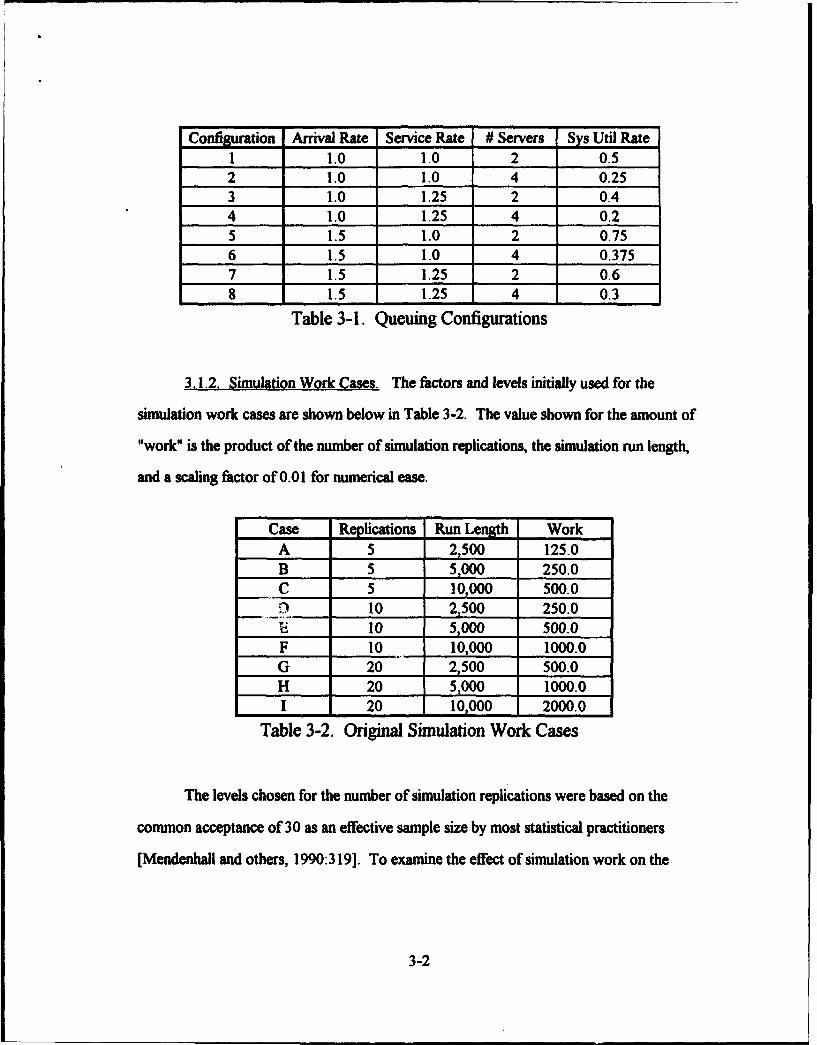
3.1.1. Oueuing Configurations. The factors and levels used for the queuing

configurations are shown below in Table 3-1. Also shown in the table is the system

utilization rate for each configuration. The configurations shown in Table 3-1 represent a

Full Factorial Design as described in Chapter 2.

3-1

Configuration Arrival Rate Service Rate # Servers Sys Util Rate1 1.0 1.0 2 0.52 1.0 1.0 4 0.253 1.0 1.25 2 0.44 1.0 1.25 4 0.25 1.5 1.0 2 0.756 1.5 1.0 4 0.3757 1.5 1.25 2 0.68 1.5 1.25 4 0.3

Table 3-1. Queuing Configurations

3.1.2. Simulation Work Cases. The factors and levels initially used for the

simulation work cases are shown below in Table 3-2. The value shown for the amount of

"work" is the product of the number of simulation replications, the simulation run length,

and a scaling factor of 0.01 for numerical ease.

Case Replications Run Length WorkA 5 2,500 125.0B 5 5,000 250.0C 5 10,000 500.05) 10 2,500 250.0E 10 5,000 500.0F 10 10,000 1000.0G 20 2,500 500.0H 20 5,000 1000.0I 20 10,000 2000.0

Table 3-2. Original Simulation Work Cases

The levels chosen for the number of simulation replications were based on the

common acceptance of 30 as an effective sample size by most statistical practitioners

[Mendenhall and others, 1990:319]. To examine the effect of simulation work on the

3-2

statistical quality of the metamodel estimates, this study considered sample sizes less than

30. The specific levels for replications were set to 5, 10, and 20.

The levels chosen for the simulation length were based on Nelson's heuristic

regarding the simulation length required to overcome the initial-transient conditions.

Nelson recommends using a simulation length of 20 times the length of the initial transient

in a simulation environment with multiple replications [Nelson, 1992:130]. Initial data

analysis of these queuing simulations indicated that a conservative estimate for the initial

transient period was 500 time units. Thus, the "acceptable" run length was set to 10,000

time units. Since it increasing the simulation run length would only serve to improve an

already acceptable simulation estimate, this study focused on run lengths not exceeding

10,000 time units. The factor levels for run length were set to 2,500, 5,000, and 10,000.

Prior to data analysis, it was determined that an effective sample of these cases

would include those cases with factors set to either their high or low levels and the case

using the middle level for each factor. These cases were A, C, E, G, and I. Based on

initial analysis of the simulation data from Cases A and C, however, further investigation

of these cases was deemed appropriate since the observed residual statistics for Case A

were better than those from Case C -- better, in the sense that the mean, standard error,

and range were all lower for Case A than for Case C. This was inconsistent with the

conjecture that more simulation resulted in better simulation estimates since estimates

from Case C were calculated using 4 times more simulation work than estimates from

Case A. With no tractable explanation for this observation readily available, additional

cases of simulation work were created using 5 replications and various run lengths.

Accordingly, 3 additional cases were added with simulation lengths less than 2,500 and I

additional case was added with simulation length greater than 10,000. The final simulation

work cases are shown in Table 3-3.

3-3

Case Replications Run Length WorkAl 5 1,000 50.0A2 5 1,250 62.5A3 5 1,500 75.0A 5 2,500 125.0C 5 10,000 500.0E 10 5,000 500.0G 20 2,500 500.0Cl 5 20,000 1,000.0I 20 10,000 2,000.0

Table 3-3. Final Simulation Work Cases

3.1.3. Summary. M/M/k queues were simulated for 8 different queuing

configurations and 9 different cases of simulation work. Estimates from the simulation

and metamodels, described later, were calculated for each of these cases of simulation

work.

3.2. Analytical Solutions

Analytical solutions for the M/M/k queues are widely available for a number of

performance measures. As noted previously, this research focused on the average queue

length for each simulation, Lq. The computations for Lq were made using following

definitions and calculations [Turban and Meredith, 1991:717-7231:

Lq = P(0)pkP the average queue length, wherek!( -_p) I

p(0)= Pk + kl-/ ,) i - -1, the probability of finding the system idle

p = Utilization factor of the single facility system -

3-4

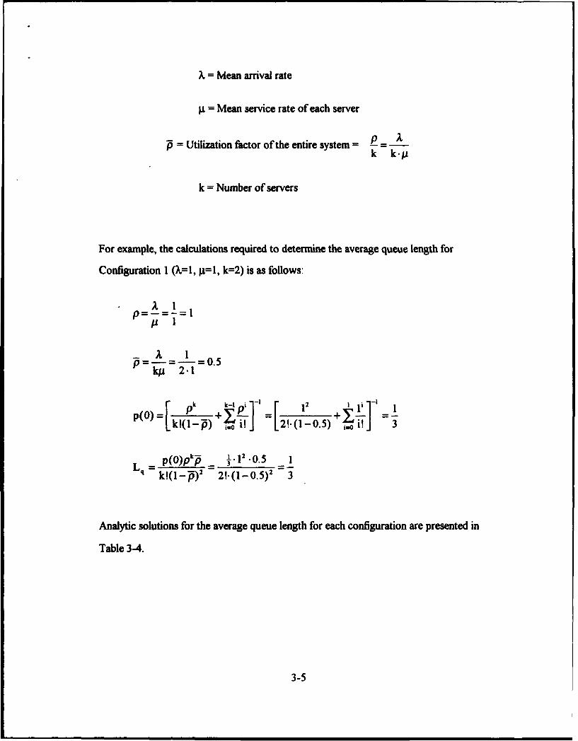
X = Mean arrival rate

g = Mean service rate of each server

= Utilization factor of the entire system = _k k.M

k = Number of servers

For example, the calculations required to determine the average queue length for

Configuration I (X=1, gt=l, k=-2) is as follows:

p•1

A 1P=-

P(O)[kP1 ) + k-' P 12!.lI.)~T[ p, Y -, r'[ 1 r 1

p(OpI ,. 12 .0.5 1Lq = _p( )2k -3~I..

k!(I-_) 2 2,.(1i0.5)2 3

Analytic solutions for the average queue length for each configuration are presented in

Table 3-4.

3-5

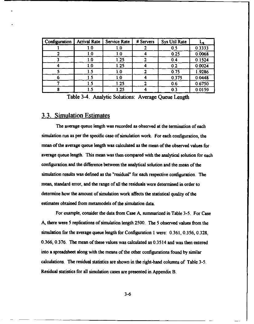
Configuration Arrival Rate Service Rate # Servers Sys Util Rate Lq1 1.0 1.0 2 0.5 0.33332 1.0 1.0 4 0.25 0.00683 1.0 1.25 2 0.4 0.15244 1.0 1.25 4 0.2 0.00245 1.5 1.0 2 0.75 1.92866 1.5 1.0 4 0.375 0.04487 1.5 1.25 2 0.6 0.67508 1.5 1.25 4 0.3 0.0159

Table 3-4. Analytic Solutions: Average Queue Length

3.3. Simulation EstimatesThe average queue length was recorded as observed at the termination of each

simulation run as per the specific case of simulation work. For each configuration, the

mean of the average queue length was calculated as the mean of the observed values for

average queue length. This mean was then compared with the analytical solution for each

configuration and the difference between the analytical solution and the mean of the

simulation results was defined as the "residual" for each respective configuration. The

mean, standard error, and the range of all the residuals were determined in order to

determine how the amount of simulation work affects the statistical quality of the

estimates obtained from metamodels of the simulation data.

For example, consider the data from Case A, summarized in Table 3-5. For Case

A, there were 5 replications of simulation length 2500. The 5 observed values from the

simulation for the average queue length for Configuration I were: 0.361, 0.356, 0.328,

0.366, 0.376. The mean of these values was calculated as 0.3514 and was then entered

into a spreadsheet along with the means of the other configurations found by similar

calculations. The residual statistics are shown in the right-hand columns of Table 3-5.

Residual statistics for all simulation cases are presented in Appendix B.

3-6

Analytic Sim Rel£2oaf Sys Util Jj Estimate Residual lResiduall Err 0/0 Residual Statistics

1 0.5 0.3333 0.3514 -0.0181 0.0181 5.43 Mean -0.00412 0.25 0.0068 0.0058 0.0010 0.0010 14.71 Sid Error 0.00823 0.4 0.1524 0.1566 -0.0042 0.0042 2.76 Median -0.00134 0.2 0.0024 0.0034 -0.0010 0.0010 1.67 Mode #N/A5 0.75 1.9286 1.8922 0.0364 0.0364 1.89 Std Dev 0.023 16 0.375 0.0448 0.0434 0.0014 0.0014 3.13 Variance 0.00057 0.6 0.6750 0.7218 -0.0468 0.0468 6.93 Kurtosis 2.40298 0.3 0.0159 0.0174 -0.0015 0.0015 9.43 Skewness -0.2139

Range 0.0832ICol Mean -0.0041 0.0138 5.74 Minimum -0.0468

Maximum 0.0364Sum -0.0328

_Count 8

Table 3-5. Simulation Results: Example Data, Case A

3.4. Metamodel Estimates

As described in previous chapters, the metamodels were fit to the data from each

case of simulation work. Metamodel specification was varied by using a linear and

logarithmic metamodels - the "basic metamodels." In addition, two other variations of

the basic metamodels were made based on data considerations.

The first variation was made by using the fill and fractional design principles

discussed in Chapter 2. The linear and logarithmic metamodels fit to data from all 8

configurations were denoted as "Full Linear" and "Full Logarithmic," respectively.

Fractional metamodels were formed by fitting the data from only 4 of the configurations.

The fractional factorial design was chosen by using the three-factor interaction as the

block generator [Box and Draper, 1987:148-152]. Both fractions are shown in Table 3-6.

The range of system utilization rates for Fraction I was 0.4 and the range for Fraction 2

was 0.50. Of the two resulting half-fractions, Fraction 2 was chosen since it represented

the greatest range of system utilization rates. Though somewhat arbitrary, this was the

3-7

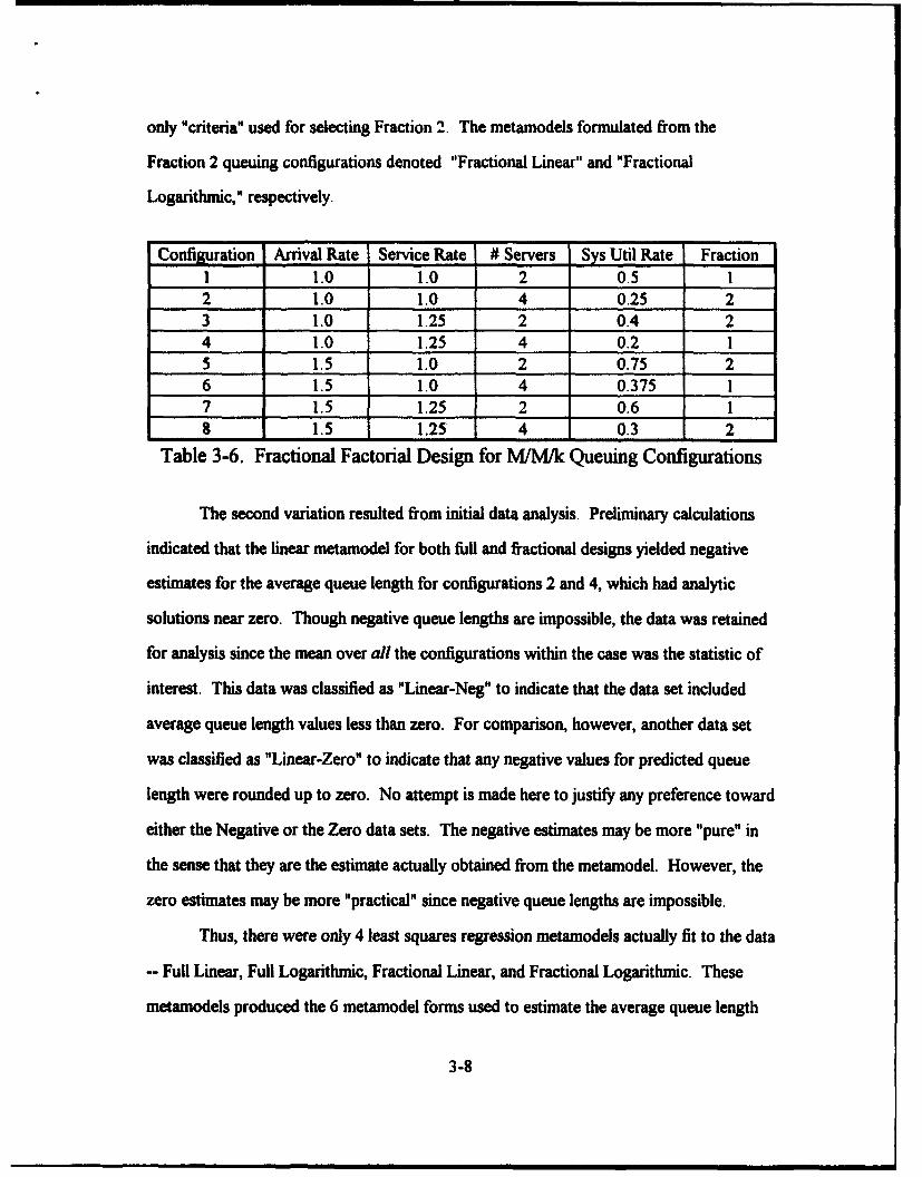
only "criteria" used for selecting Fraction 2. The metamodels formulated from the

Fraction 2 queuing configurations denoted "Fractional Linear" and "Fractional

Logarithmic," respectively.

Configuration Arrival Rate Service Rate # Servers Sys Util Rate Fraction1 1.0 1.0 2 0.5 12 1.0 1.0 4 0.25 23 1.0 1.25 2 0.4 24 1.0 1.25 4 0.2 15 1.5 1.0 2 0.75 26 1.5 1.0 4 0.375 17 1.5 1.25 2 0.6 18 1.5 1.25 4 0.3 2

Table 3-6. Fractional Factorial Design for M/M/k Queuing Configurations

The second variation resulted from initial data analysis. Preliminary calculations

indicated that the linear metamodel for both full and fractional designs yielded negative

estimates for the average queue length for configurations 2 and 4, which had analytic

solutions near zero. Though negative queue lengths are impossible, the data was retained

for analysis since the mean over all the configurations within the case was the statistic of

interest. This data was classified as "Linear-Neg" to indicate that the data set included

average queue length values less than zero. For comparison, however, another data set

was classified as "Linear-Zero" to indicate that any negative values for predicted queue

length were rounded up to zero. No attempt is made here to justify any preference toward

either the Negative or the Zero data sets. The negative estimates may be more "pure" in

the sense that they are the estimate actually obtained from the metamodel. However, the

zero estimates may be more "practical" since negative queue lengths are impossible.

Thus, there were only 4 least squares regression metamodels actually fit to the data

-- Full Linear, Full Logarithmic, Fractional Linear, and Fractional Logarithmic. These

metamodels produced the 6 metamodel forms used to estimate the average queue length

3-8

for each configuration when the additional distinction between the negative and zero

estimates were taken into account -- Full Linear-Neg, Full Linear-Zero, Full Logarithmic,

Fractional Linear-Neg, Fractional Linear-Zero, and Fractional Logarithmic.

The functional forms of the basic metamodels are shown in Table 3-7 using the

definitions given in Chapter 2. The 4 least squares regression metamodels for each case

Metamodel Type Metamodel Form

Linear Lq = P0 + Arr • P, + Svc. -P + Num. 3A

Logarithmic Lq = eps ( AS 0-' or

ln(Lq) = -0 + P,• In(Arr) - P. ln(Svc) - P3" In(Num)

Table 3-7. Predictive Metamodel Forms

of simulation work were developed using Statistical Analysis System (SAS) least squares

regression routines. For the linear metamodels, inputs to the regression models were the

average queue length, arrival rate, service rate, and number of servers for each respective

configuration. The logarithmic model used the logarithms of the same inputs. The

resulting metamodel coefficients from the SAS output for both metamodels were

transformed into their respective finctional form such that the average queue length was

estimated.

For example, in the formulation of the full metamodels for Case A, there were 8

simulation configurations evaluated with 5 replications, so there were 40 (8 x 5 = 40)

observations of the average queue length used to calculate the least squares regression

coefficients used in the metamodels. The regression coefficients are displayed as part of

the SAS output for each model. Example SAS printouts for both the Full Linear and the

Full Logarithmic models are shown in Tables 3-8 and 3-9, respectively.

3-9

Analysis of Variance

Sum of MeanSource DF Squares Square F Value Prob>F

Model 3 9.94504 3.31501 21.833 0.0001Error 36 5.46595 0.15183C Total 39 15.41099

Root MSE 0.38966 R-square 0.6453Dep Mean 0.39900 A4j R-sq 0.6158C.V. 97.65820

Parameter Estimates

Parameter Standard T for HO:Variable DF Estimate Error Parameter-0 Prob > III

INTERCEP 1 1.762800 0.66356063 2.657 0.0117ARRIVAL 1 1.078800 0.24644023 4.378 0.0001SERVICE 1 -1.393600 0.49288046 -2.827 0.0076NUMBER 1 -0.381500 0.06161006 -6.192 0.0001

Table 3-8. Example SAS Output: Full Linear Metamodel, Case A

Analysis of Variance

Sum of MeanSource DF Squares Square F Value Prob>F

Model 3 187.81476 62.60492 938.910 0.0001Error 36 2.40042 0.06668C Total 39 190.21518

Root MSE 0.25822 R-square 0.9874Dep Mean -2.59946 Adj R-aq 0.9863C.V. -9.93366

Paramet Estimates

Parameter Standard T for HO:Variable DF Estimate Error Parameter=0 Prob > PT

INTERCEP 1 2.780640 0.14143366 19.660 0.0001LOGARR 1 4.255964 0.20139036 21.133 0.0001LOGSERV 1 -3.628686 0.36593826 -9.916 0.0001LOGNUM 1 -5.615028 0.11780581 -47.663 0.0001

Table 3-9. Example SAS Output: Full Logarithmic Metamodel, Case A

The coefficients from the least squares regression were used in their respective

models to estimate the value of the average queue length for each configuration in each

3-10

case for each metamodel type. The Full Linear metamodel estimation for Case A,

Configuration I was calculated as follows:

Lq = PO + (01" Arr) + (A" Svc) + (A. Num)Lq = 1.7628 + (1.0788.1) + (-1.3936.1) + (-0.3815.2)

Lq = 0.6850

The Full Logarithmic metamodel estimation for Case A, Configuration 1 was calculated as

follows, after multiplying the SAS coefficients for I and N by a factor of-I:

ln(Lq) = P30 + P" ln(Arr) - A2 • ln(Svc) -13 ln(Num)

ln(Lq) = 2.7806+ 4.2560. ln(l) - 3.6287. ln(l) - 5.6150. ln(2)

In(Lq) = 2.7806+ 0+ 0- 3.8920

ln(Lq) =-1.1114Lq =.3291

Recall that for Configuration 1, the analytic solution for the Average Queue Length was

0.3333.

As with the simulation results, these metamodel estimates were compared to the

analytical solution, residuals calculations made, and descriptive statistics of the residuals

were calculated for the entire case. Examples of residual statistic data for Case A are

shown in Table 3-10a for the Full Linear-Neg metamodel, Table 3-10b for the Full Linear-

Zero metamodel, and Table 3-10c for the Full Logarithmic metamodel. In each table, the

metamodel estimates for Configuration 1 are shaded.

3-11

Analytic Meta Re]Config Sys Util IA Estimate Residual lResiduall Err (1/) Residual Statistics

1 0.5 0.3333 0.6850 -0.3517 0.3517 105.52 Mean -0.00412 0.25 0.0068 -0.0780 0.0848 0.0848 1247.06 Std Error 0.13813 0.4 0.1524 0.3366 -0.1842 0.1842 120.87 Median -0.14074 0.2 0.0024 -0.4264 0.4288 0.4288 17866.67 Mode #N/A5 0.75 1.9286 1.2244 0.7042 0.7042 36.51 Std Dev 0.39066 0.375 0.0448 0.4614 -0.4166 0.4166 929.91 Variance 0.15257 0.6 0.6750 0.8760 -0.2010 0.2010 29.78 Kurtosis 0.00718 0.3 0.0159 0.1130 -0.0971 0.0971 610.69 Skewness 0.9933

Range 1.1208IColMeanj -0.0041 0.3086 12618.381 Minimum -0.4166

Maximum 0.7042

Sum -0.0328Count 8

Table 3-10a. Example Data: Full Linear-Neg Metamodel Residual Statistics,Case A

Analytic Meta RelConfig Sys Util Lq Estimate Residual IResiduall Err (%) Residual Statistics

1 0.5 0.3333 0.6850 -0.3517 0.3517 105.52 Mean -0.06722 0.25 0.0068 0.0000 0.0068 0.0068 100.00 Std Error 0.12253 0.4 0.1524 0.3366 -0.1842 0 1842 120.87 Median -0.14074 0.2 0.0024 0.0000 0.0024 0.0024 100.00 Mode #N/A5 0.75 1.9286 1.2244 0.7042 0.7042 36.51 Std Dev 0.34666 0.375 0.0448 0.4614 -0.4166 0.4166 929.91 Variance 0.12017 0.6 0.6750 0.8760 -0.2010 0.2010 29.78 Kurtosis 4.03438 0.3 0.0159 0.1130 -0.0971 0.0971 610.69 Skewness 1.7839

Range 1.1208ICol Meanl -0.0672 0.2455 ]254.16-1 Minimum -0.4166


_Count 8

Table 3-10b. Example Data: Full Linear-Zero Metamodel ResidualStatistics, Case A

3-12

Analytic Meta RelCofi Sys Util Lq Estimate Residual Residuall Err (1/) Residual Statistics

1 0.5 0.3333 0.3291 0.0042 0.0042 1.26 Mean -0.00642 0.25 0.0068 0.0067 0.0001 0.0001 1.47 Std Error 0.02233 0.4 0.1524 0.1464 0.0060 0.0060 3.94 Median 0.00214 0.2 0.0024 0.0030 -0.0006 0.0006 25.00 Mode #N/A5 0.75 1.9286 1.8482 0.0804 0.0804 4.17 Std Dev 0.06326 0.375 0.0448 0.0377 0.0071 0.0071 15.85 Variance 0.00407 0.6 0.6750 0.8224 -0.1474 0.1474 21.84 Kurtosis 4.81108 0.3 0.0159 0.0168 -0.0009 0.0009 5.66 Skewness -1.6170

Range 0.2278[Col Meanj -0.0064 0.0308 9.90 Minimum -0.1474


_Count 8

Table 3-10c. Example Data: Full Logarithmic Metamodel Residual

Statistics, Case A

Though the fractional metamodels were formulated differently than the full metamodels,

the fractional metamodel estimates and residual statistics were calculated in a similar

manner as the full metamodels shown above and identical residual analysis was performed

for the residual statistics from the fractional metamodels.

3.5. Residual Analysis

The residual statistics (mean, standard error, and range) were calculated for case

of simulation work for each of the seven respective estimation types: Simulation, Full

Linear-Neg metamodel, Full Linear-Zero metamodel, Full Logarithmic metamodel,

Fractional Linear-Neg metamodel, Fractional Linear-Zero metamodel, and Fractional

Logarithmic metamodel. Graphic comparisons and Single-Factor Analysis of Variance

(ANOVA) calculations were made for each residual statistic in order to determine if the

residual statistics were affected by the case of simulation work or the metamodel type. An

example of these calculations within a case are shown in the shaded portion of the row in

3-13

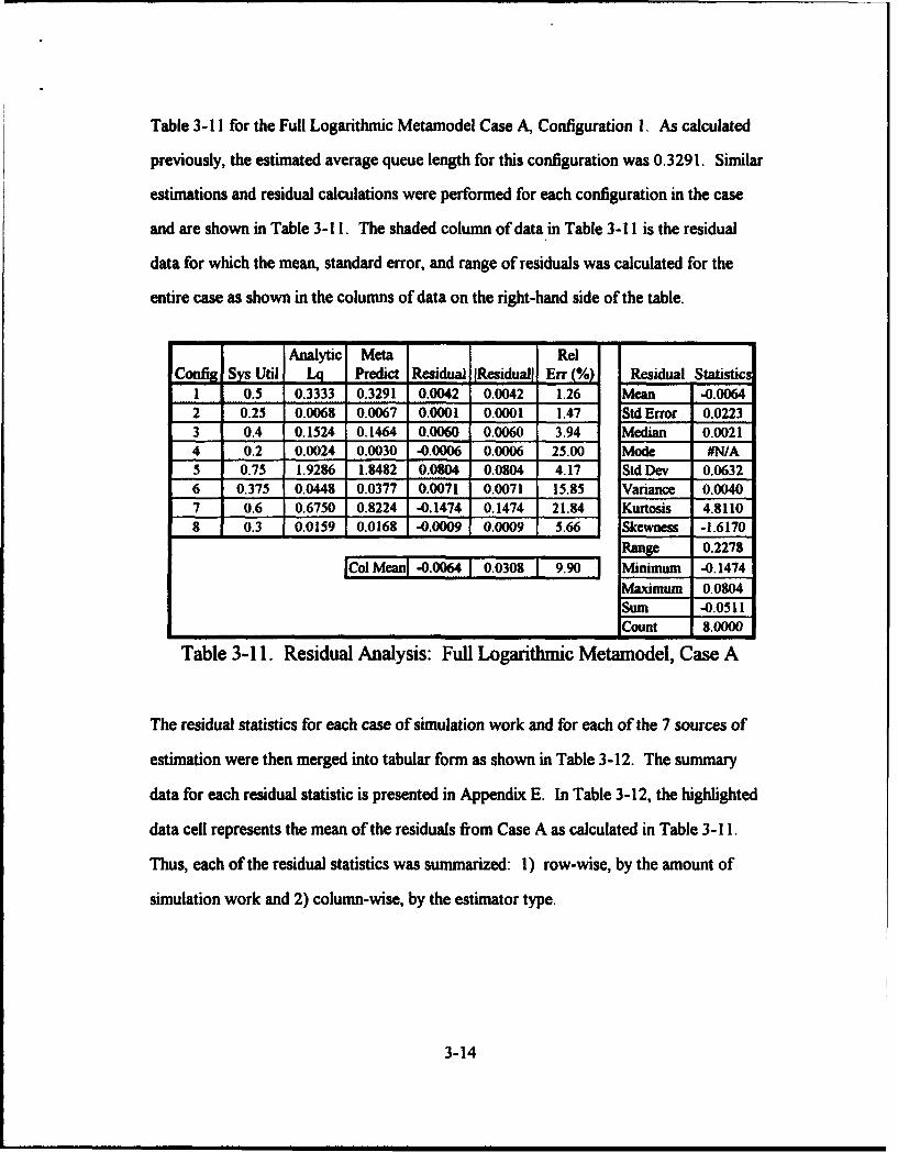
Table 3-11 for the Full Logarithmic Metamodel Case A, Configuration 1. As calculated

previously, the estimated average queue length for this configuration was 0.3291. Similar

estimations and residual calculations were performed for each configuration in the case

and are shown in Table 3-11. The shaded column of data in Table 3-11 is the residual

data for which the mean, standard error, and range of residuals was calculated for the

entire case as shown in the columns of data on the right-hand side of the table.

Analytic Meta Rel

Confi Sys Uti Lq Predict Residual Rsidual Err(%) Statistics1 0.5 0.3333 0.3291 0.0042 0.0042 1.26 Mean -0.0064

fi~ ~ 0.00 14

0.25 0.0068 0.0067 0.0001 0.0001 1.47 Std Error 0.02233 0.4 0.1524 0.1464 0.0060 0.0060 3.94 Median 0.00214 0.2 0.0024 0.0030 -0.0006 0.0006 25.00 Mode #N/A5 0.75 1.9286 1.8482 0.0804 0.0804 4.17 Std Dev 0.06326 0.375 0.0448 0.0377 0.0071 0.0071 15.85 Variance 0.00407 0.6 0.6750 0.8224 -0.1474 0.1474 21.84 Kurtosis 4.81108 0.3 0.0159 0.0168 -0.0009 0.0009 5.66 Skewness -1.6170

Range 0.2278Col Mean -0.0064 0.0308 9.90 Minimum -0.1474

Maximum 0.0804Sum -0.0511Count 8.0000

Table 3-11. Residual Analysis: Full Logarithmic Metamodel, Case A

The residual statistics for each case of simulation work and for each of the 7 sources of

estimation were then merged into tabular form as shown in Table 3-12. The summary

data for each residual statistic is presented in Appendix E. In Table 3-12, the highlighted

data cell represents the mean of the residuals from Case A as calculated in Table 3-11.

Thus, each of the residual statistics was summarized: 1) row-wise, by the amount of

simulation work and 2) column-wise, by the estimator type.

3-14

Full Full Frac FracWork Simulation Lin-Neg Lm-Zero Full Log Lm-Neg Lin-Zero Frac Log

Al: 50 0.0305 0.0305 -0.0268 -0.0068 -0.0775 -0.1722 -0.0193A2: 62.5 -0.0102 0.0025 -0.0729 -0.0257 -0.1478 -0.2615 -0.045A3: 75 0.0093 0.0093 -0.0532 -0.0152 -0.1026 -0.2030 -0.0071A: 125 -0.0041 -0.0041 -0.0675 -0.0064 -0.1220 -0.2301 -0.0215C: 500 0.0208 0.0209 -0.0379 -0.0053 -0.0931 -0.1937 0.0053E: 500 0.0058 0.0058 -0.0563 -0.0081 -0.1203 -0.2279 -0.0122G: 500 0.0037 0.0037 -0.0594 -0.0169 -0.1317 -0.2419 -0.0116C1: 1000 0.0040 0.0039 -0.0572 -0.0202 -0.1265 -0.2336 -0.02371: 2000 -0.0011 -0.0111 -0.0653 -0.0226 -0.1321 -0.2421 -0.0215

Table 3-12. Residual Analysis: Mean of Residuals from Simulation and AllMetamodels

3.6: Summary

The experimental design for this research was structured to investigate the effects

of simulation work and metamodel specification on the average queue length estimates

from the resulting metamodels. The 8 queuing configurations provided the basis for

functionally relating the customer arrival rate, the service rate, and the number of servers

to the average queue length in the form of a metamodel. The nine levels of simulation

work, two metamodel forms (linear and logarithmic), and two levels of fractionation

resulted in a 9 x 2 x 2 factorial experimental design. The results of the experiment and the

corresponding analysis are presented in the following chapter.

3-15

4. Results and Analysis

4.0. IntroductionThe experiment was conducted as presented in Chapter 3 and residuals were

analyzed for each case of simulation work. Analysis of these residuals was used to

determine if the amount of simulation work affected the statistical quality of estimates of

average queue length obtained from metamodels of the simulation data. Specifically, this

analysis was done in two ways. First, by a graphic comparison of the residual statistic

data for all estimation types. Secondly, a Single-Factor ANOVA on each set of residual

statistic data from the different metamodels was performed to determine if the different

cases of simulation work yielded similar residual statistics and to determine if the different

metamodel types yielded similar residual statistics.

The graphic analysis for the residual statistics is presented in Section 4.1. The

ANOVA results for residual statistics are presented in Section 4.2. In addition to the

simulation and metamodel residual analysis, the R2 values from the Full Linear, Full

Logarithmic, Fractional Linear, and Fractional Logarithmic metamodels were graphi; ally

compared. These results are presented in Section 4.3.

4.1. Graphic Analysis

4.1.0. Introduction. A summary of the residual data for each statistic and

respective estimation type is presented in Appendix E. The corresponding graphs and

summaries of the residual statistics are presented in Section 4. 1. 1. through Section 4.1.3.

4. 1. 1. Mean of Residuals. The graph of the mean of the residuals from the

simulation and all the metamodels is shown in Figure 4-1.

4-1

Figure 4-1. Mean of Residuals for Simulation and All Metamodelsvs. Simulation Work

-0-simubM ---6-d LA ---- FU LiAnN -0FUN Lia-Z -E- F•a LMo -6- Fr •n-N -. F LI-Z

03

025

0.2

0.15

0.1

0.05

0

-0.05

-0.15 -- - - - ~- - -- ---6a-0.15 - "a

.0.25 ' . -

-0.3

Al A2 A3 A C E G Cl I50 62.5 75 125 500 500 500 1000 2000

The effect of simulation work and metamodel specification on the mean of residuals was

observed in two ways. First, the effect of simulation work was observed by examining the

graph of any single estimation source -- either simulation or any of the metamodel forms.

It is apparent that the mean of the residuals does not change as the amount of work as

increases for any given estimator. For example, the graph corresponding to the mean of

residuals from the Fractional Linear-Zero metamodel is relatively straight from left to right

over the entire range of simulation work cases. Although there was some apparent

fluctuation corresponding to the residual means from Cases A! and A2, it should be noted

that Case I is effectively the point at which traditional statistical inference begins -- Case I

was the combination of 20 replications and simulation length 10,000 time units. Thus, the

apparent deviations for Cases Al and A2 were not deemed significant based on this

4-2

graphical analysis since they represent extreme "worst case" scenarios in this research.

The remaining cases are did not demonstrate this degree of variation. Secondly, the effect

of metamodel specification was observed by examining the graph at any level of simulation

work. It is apparent that for any case of simulation work chosen, there was a difference in

the mean of the residuals. For example, in Case C, 6 of the 7 observed values for the

mean of the residuals are clearly distinguishable in this graph.

4.1.2. Standard Error of Residuals. The graph of the standard error of the

residuals from the simulation and all the metamodels is shown in Figure 4-2. The effect of

simulation work and metamodel specification on the standard error of residuals was

observed as previously described in Section 4. 1. 1.

Figure 4-2. Standard Error of Residuals for Simulation and AllMetamodels vs. Simulation Work

F--*- ----- Fu Los -A-F.UNLa-N -- Fug Lh-z -O-FmLAS - .-FmU,-N -0- R- -Z

0.3

0.25

0.2 - -ja - - - ---. ~ - ---- ---------- --- -- - --0.12 + ,

0.15 - A_ A_ A A, A A A ,0 4- . --- -1----.-..

0.15

0.0

Al A2 A3 A C E G CI I50 62.5 75 125 500 500 500 1000 2000

4-3

Again, it is apparent that the standard error of the residuals did not change

appreciably as the amount of work was increased for the specific estimator. For example,

the graph corresponding to the standard error of residuals from the Full Logarithmic

metamodel is relatively straight from left to right over the entire range of simulation work

cases. The apparent fluctuation corresponding to the standard error of the residuals from

Cases Al and A2 is only observed for the Fractional Logarithmic metamodel. Again,

these apparent deviations for Cases AI and A2 were not deemed significant based on this

graphical analysis since they represent extreme "worst case" scenarios in this research and

the remaining cases did not demonstrate this characteristic.

Secondly, the examination of the graph at any level of simulation work yields

similar results as before. It is apparent that for any case of simulation work chosen there

was a difference in the standard error of the residuals. For example, at almost all of the 9

cases of simulation work, the observed values for the standard error of the residuals are

clearly distinguishable in this graph.

In addition, it is evident that the Full and Fractional Logarithmic metamodel

estimates produced standard errors that best approximated the standard errors from the

simulation estimates and confirms Friedman and Friedman's validation of the logarithmic

metamodels for estimating the average queue length of M/M/k queues.

4.1.3. Range of Residuals. The graph of the range of the residuals from the

simulation and all the metamodels is shown in Figure 4-3. The effect of simulation work

and metamodel specification on the range of residuals was observed as previously

described in Section 4. 1. 1.

4-4

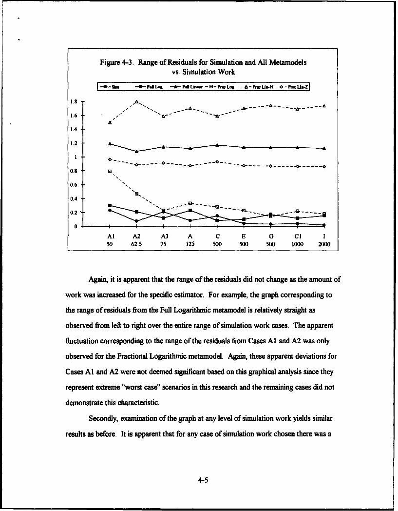
Figure 4-3. Range of Residuals for Simulation and All Metamodels

vs. Simulation Work

--*-Sim --- F".LA* ---- uA- MLU -8--Fm Us -F6,-.N -F-F 0 - zF

1.8 - •- ...-- - --- A-A

1.6

1.4

1.2

1 ------- 0 -- ---0-- 0

0.8

0.6

0.4

Al A2 A3 A C E G Cl I50 62.5 75 125 500 500 500 1000 2000

Again, it is apparent that the range of the residuals did not change as the amount of

work was increased for the specific estimator. For example, the graph corresponding to

the range of residuals from the Full Logarithmic metamodel is relatively straight as

observed from left to right over the entire range of simulation work cases. The apparent

fluctuation corresponding to the range of the residuals from Cases Al and A2 was only

observed for the Fractional Logarithmic metamodel. Again, these apparent deviations for

Cases Al and A2 were not deemed significant based on this graphical analysis since they

represent extreme "worst case" scenarios in this research and the remaining cases did not

demonstrate this characteristic.

Secondly, examination of the graph at any level of simulation work yields similar

results as before. It is apparent that for any case of simulation work chosen there was a

4-5

difference in the range of the residuals. For example, at all of the 9 cases of simulation

work, the observed values for the range of the residuals are clearly distinguishable in this

graph.

In addition, it is evident that the Full and Fractional Logarithmic metamodel

estimates produced ranges that best approximated those from the simulation estimates and

confirms Friedman and Friedman's validation of the logarithmic metamodels for estimating

the average queue length of M/M/k queues.

4.1.4. Summary of Graphic Analysis. It is apparent from the graphs of the

residual statistic data that differences in the means, standard errors, and ranges of the

residuals were not due to the amount of simulation work in the metamodels. In addition,

it is apparent from these graphs that differences were due to the metamodel used to

estimate the average queue length.

4.2. Single-Factor ANOVA

4.2.0. Introduction. Single-Factor ANOVA was performed on the metamodel

data to determine the effects of simulation work on the statistical quality of estimates

obtained from metamodels of the simulation data. For each residual statistic, a set of data

was collected as shown previously for the residual means in Table 3-12. ANOVA

calculations and F-tests were performed on the data in two ways. First, a row-wise test

was used to determine if any of the respective residual statistics from metamodel estimates

were significantly different between the different cases of simulation work - do the

residuals vary based on the level of simulation work? Secondly, a column-wise test was

used to determine if any of the respective residual statistics from metamodel estimates

were significantly different between the different metamodel types - do the residuals vary

based on metamodel specification?

4-6

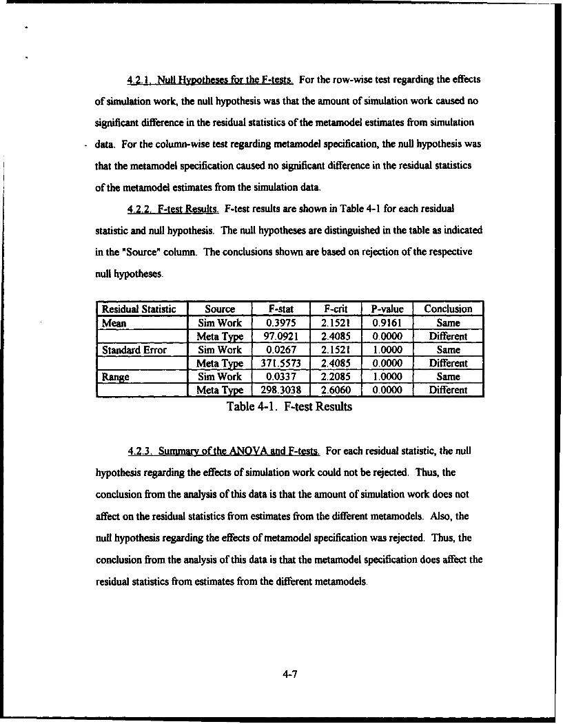
4.2. 1. Null Hypotheses for the F-tests. For the row-wise test regarding the effects

of simulation work, the null hypothesis was that the amount of simulation work caused no

significant difference in the residual statistics of the metamodel estimates from simulation

data. For the column-wise test regarding metamodel specification, the null hypothesis was

that the metamodel specification caused no significant difference in the residual statistics

of the metamodel estimates from the simulation data.

4.2.2. F-test Results. F-test results are shown in Table 4-1 for each residual

statistic and null hypothesis. The null hypotheses are distinguished in the table as indicated

in the "Source" column. The conclusions shown are based on rejection of the respective

null hypotheses.

Residual Statistic Source F-stat F-crit P-value ConclusionMean Sim Work 0.3975 2.1521 0.9161 Same

Meta Type 97.0921 2.4085 0.0000 DifferentStandard Error Sim Work 0.0267 2.1521 1.0000 Same

Meta Type 371.5573 2.4085 0.0000 DifferentRange Sim Work 0.0337 2.2085 1.0000 Same

Meta Type 298.3038 2.6060 0.0000 Different

Table 4-1. F-test Results

4.2.3. Summary of the ANOVA and F-tests. For each residual statistic, the null

hypothesis regarding the effects of simulation work could not be rejected. Thus, the

conclusion from the analysis of this data is that the amount of simulation work does not

affect on the residual statistics from estimates from the different metamodels. Also, the

null hypothesis regarding the effects of metamodel specification was rejected. Thus, the

conclusion from the analysis of this data is that the metamodel specification does affect the

residual statistics from estimates from the different metamodels.

4-7

4.3. Metamodel Comparison.

The SAS output used in calculating the respective metamodel coefficients included

R2 values for each metamodel. Consequently, a comparison was made of the R2 values for

the different metamodels. For example, the R2 statistic for the Case A, Full Linear

Metamodel is 0.6453 as shown in the example SAS output of Table 3-8. Data for all

metamodels is presented in Appendix F. A graphical summary is shown in Figure 4-4.

This graph shows that the Full Logarithmic and both Fractional Metamodels have similar

R2 values, approximately 0.94 and higher. In addition, the Full Linear Metamodel has a

distinctly lower R2 value of approximately 0.64.

Friedman and Friedman's research produced an R2 value of 0.74 for their validated

logarithmic model. The relative disparity between the best case from this research, the

Full Logarithmic metamodel with an approximate R2 = 0.94 and the Friedman and

Friedman logarithmic metamodel may be due to the fitting the respective metamodels to

different sets of simulation data. The range of system utilization rates for this research

was from 0.2 to 0.75. The Friedman and Friedman experimental design resulted in a range

of 0.90 to 0.95. Although the lack of fit of their linear metamodel was discussed in their

research, no R2 values for their linear metamodel were given [Friedman and Friedman,

1985:145].

4-8

Figure 4-4. R-Squared Values, Full and Fractional Metamodels

-Ful Log - Fu Lia- Fin Log - Fc Unse

0.9

0.8

0.7 -

0.6 -

OA03 4-

0.4

0.2 4.

0.1

Al A2 A3 A C E G CI I

4.4. Summary

The graphic analysis and the results from the F-tests provide convincing evidence

that the amount of simulation work does not affect on the residual statistics from estimates

from the different metamodels and that the metamodel specification does affect the

residual statistics from estimates from the different metamodels. Analysis of the

metamodel R2 data is consistent with Friedman and Friedman's research with respect to

the difference between the R2 values for the Full Logarithmic and the Full Linear

metamodels. No inference is made regarding the R2 values for the fractional metamodels.

4-9

5. Conclusions and Recommendations

5.0. IntroductionAs stated previously, the purpose of this research was to determine how the

amount of simulation work affects the statistical quality of the estimates obtained from

metamodels of the simulation data. Conclusions from the preceding chapters are

formalized here. In addition, recommendations for additional research are presented

5.1. ConclusionsThe graphical analysis and ANOVA analysis in Chapter 4 clearly address the

problem statement and research objective stated in Chapter 1. Specifically, the amount of

simulation work has no significant effect on the statistical quality of the estimates

obtained from metamodels of the simulation data. Also, the metamodel specification has

a significant effect on the statistical quality of the estimates obtair,)d from metamodels of

the simulation data.

Though the conclusion regarding the effect of simulation work is somewhat

counter-intuitive, it is supported by graphic analysis and rather conclusive F-tests. The

conclusion regarding the effect of metamodel specification is also supported by graphic

analysis and rather conclusive F-tests. It confirms intuition regarding metamodel

specification and also confirms the research findings of Friedman and Friedman.

Based on this research, it would seem more prudent to develop a better specified

metamodel than to simply increase the amount of simulation work in an attempt to

develop a metamodel with more predictive validity.

5-1

5.2. Recommendations

5.2.0 Introduction. Though the focus of this research was on a relatively simple

system and corresponding computer simulation, additional research is warranted in the

areas described below.

5.2.1. Queuing Networks. In many Department of Defense simulation and

metamodel applications, it is quite common that multiple simulations are used in a

hierarchical manner. For example, a one-on-one air engagement model may be used as

input to an air campaign model, which in turn, may be used as input to a theater-level

combat simulation model. If metamodels were applied to any, or all, of these "cascading"

simulations, it would be of crucial importance to know how different levels of simulation

work and different levels of metamodel specification affect the statistical quality of any

estimates gained from the simulation and or metamodels -- who won the dogfight, air

campaign, or war? To better understand the relationship of simulation work and

metamodel specification in a scenario such as this, the research presented here could be

modified to include queuing networks. In the simplest case, tandem queues could be

simulated using identical queuing configurations, cases of simulation work, and

metamodels for the purpose of estimating the average queue length. Though some of the

analytical solution procedures and metamodel prediction procedures would require slight

modification due to the nature of tandem queues, the analysis should be as straightforward

as that for single queues. In a more demanding case, the queuing configurations, work

amount, and metamodel specification could be varied Sor different queues in the network.

5.2.2. Queuing Statistics. To better understand the aingIe queues studied in this

research, other performance measures of M/M/k queues could be analyzed using the same

methodology presented in Chapter 3. This research benefited by using the validated

metamodel for estimating the average queue length as presented by Friedman and

5-2

Friedman. Further investigation of M/M/k queuing performance measures would require

validation of any metamodels used.

5.2.3. Different System. To extend the investigation of the effects of simulation

work on metamodel estimation, this methodology could be applied to a system other than

M/M/k queues. The range of potential systems under study would be limited primarily by

the requirement for a valid simulation and metamodel.

5.2.4. Fractionation and Metamodels. Just as the amount of simulation work was

used as a factor in this experiment, the effects of fractionation used in metamodel

formulation could also studied. In all likelihood, such research would involve using more

simulation configurations since the level of fractionation possible in was limited by a "full"

factorial design consisting of only 8 design points.

5.3. Summary

This research provided relatively simple conclusions. Essentially, it is better to

work smarter in developing a metamodel than it is to work harder by increasing the

amount of simulation work. Given the conclusions presented previously, further

investigation of the relationship between simulation work and metamodel estimation is

essential to establishing a bound, or "comfort zone," for analysts and decision makers who

are faced with problems involving different levels of simulation and metamodel

specification. Quite often, simulations and metamodels are used in sequence or

combination with little thought as to what happens to the quality of the "answer" provided

by one simulation as it is literally "fed" into another simulation as an input. Ultimately, an

answer emerges with untold amounts of statistical baggage acquired along the way as a

result of the multiple simulation and metamodel environments.

This research begins to address this problem and the aforementioned

recommendations should provide a basis for research whereby analysts and decision

5-3

makers can begin to understand, and hopefully avoid, any potential pitfalls of using

different amounts of simulation work and using metamodels of different specification in

their computer simulations.

5-4

Appendix A: Simulation Overview

The queuing configurations for this research were simulated using the

SLAMSYSTEM simulation language. Neither a SLAM or SLAMSYSTEM tutorial is

presented here. Interested readers are referred to Priskters text for a detailed explanation

of the SLAM simulation language and many other simulation topics. Example model

statements are shown below in Figure A-I for Configuration 1, Case A- Recall that Case

A was for 5 replications of simulation length 2,500.

Figure A-I. Example SLAMSYSTEM Model, Configuration 1, Case A

GEN,MKT,MKT META 1,12/17/93,5,Y,Y,Y/Y,Y,Y/1,132;LIMITS,1,2, 100;NETWORK;

START CREATE,EXPON(1.0,1),,,,1;ACTIVITY;QUEUE (1) ,,,;ACTIVITY(2),EXPON(1.0) ,2;COLCT,INT(1) ,TOTAL TIS;ACTIVITY,,, END;

END TERMINATE, 50000;END;

SEEDS, 61954987(1) ,75128931 (2);INITIALIZE,,2500,Y;FIN;

The seeds for all simulations were generated using Mathcad's pseudo-random number

generator for Uniformly (0, 1) distributed random deviates. All queues were simulated

A-I

using a GATEWAY 2000 personal computer, model 4DX2-50V. This particular model

had an Intel 50M-Hz 80486DX2 Mic •oprocessor and 8 MB Ram. The above simulation

model, seeds, and hardware produced average queue lengths of 0.361, 0.356, 0.328,

0.3 36, and 0.3 76. This simulation configuration and case was simulated in approximately

1:50 minutes of clock time. For comparison, Configuration I and Case 1 (20 replications

of simulation length 10,000) was simulated in approximately 18:20 minutes.

A-2

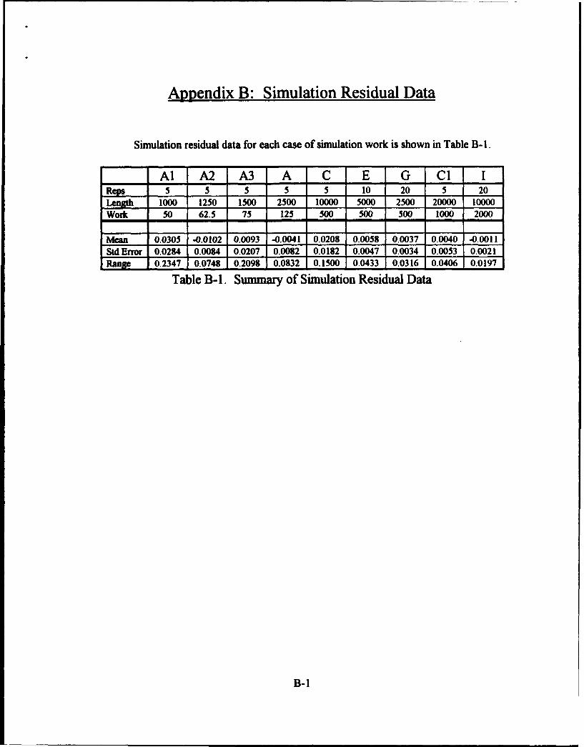
Appendix B: Simulation Residual Data

Simulation residual data for each case of simulation work is shown in Table B-1.

Al A2 A3 A C E G CI IReps 5 5 5 5 5 10 20 5 20Length 1000 1250 1500 2500 10000 5000 2500 20000 10000Work 50 62.5 75 125 500 500 500 1000 2000

Mean 0.0305 -0.0102 0.0093 -0.0041 0.0208 0.0058 0,0037 0.0040 -0.0011Std Error 0.0284 0.0084 0.0207 0.0082 0.0182 0.0047 0.0034 0.0053 0.0021Range 0.2347 0.0748 0.2098 0.0832 0.1500 0.0433 00316 0.0406 0.0197

Table B-1. Summary of Simulation Residual Data

B-I

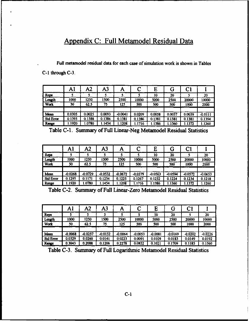
Appendix C: Full Metamodel Residual Data

Full metamodel residual data for each case of simulation work is shown in Tables

C-I through C-3.

AAl A2 A3 A C E G CI I5 5 5 5 5 10 20 5 20

1 000 1250 1500 2500 10000 5000 2500 20000 10000Work 50 62.5 75 125 500 500 500 1000 2000

Mean 0.0305 0.0025 0.0093 -0.0041 0.0209 0.0058 0.0037 0.0039 -00111Std Error 0.1395 0.1388 0.1386 0.1381 0.1386 0.1381 0.1381 0.1381 01394Ran 1.1920 1.0780 1.1454 1.1208 1.1716 1.1386 1.1360 1.1372 1.1260

Table C-1. Summary of Full Linear-Neg Metamodel Residual Statistics

Al A2 A3 A C E G Cl IR 5 5 5 5 5 10 20 5 20

1ngt 1000 1250 1500 2500 10000 5000 2500 20000 10000Work 50 62.5 75 125 500 500 500 1000 2000

Mean -0.0268 -0.0729 -0.0532 -0.0672 -0.0379 -0.0563 -0.0594 -0.0572 -0.0653Std Error 0.1295 0.1171 0.1254 0.1225 0.1267 0.1232 0.1224 0.1234 0.1218Ra1e 1.1920 1.0780 1.1454 1.1208 1.1716 1.1386 1.1360 1.1372 1.1260

Table C-2. Summary of Full Linear-Zero Metamodel Residual Statistics

Al A2 A3 A C E G CI IReps 5 5 5 5 5 10 20 5 20Length 1000 1250 1500 2500 10000 5000 2500 20000 10000Work 50 62.5 75 125 500 500 500 1000 2000

Mea -0.0068 -0.0257 -0.0152 -0.0064 -0.0053 -0.0081 -0.0169 -0.0202 -0.0226Std Error 0.0329 0.0260 0.0141 0.0223 0.0091 0.0109 0.0183 0.0149 0.0192Range 0.3043 0.2088 0.1206 0.2278 0.0852 0.1021 0.1709 0.1185 0.1560

Table C-3. Summary of Full Logarithmic Metamodel Residual Statistics

C-I

Appendix D: Fractional Metamodel Residual Data

Fractional metamodel residual data for each case of simulation work is shown in

Tables D- I through D-3.

Al A2 A3 A C E G C1 IReps 5 5 5 5 5 10 20 5 20Length 1000 1250 1500 2500 10000 5000 2500 20000 10000Work 50 62.5 75 125 500 500 500 1000 2000

Mean -0.0775 -0.1478 -0.1026 -0.1220 -0.0931 -0.1203 -0.1317 -0.1265 -0.1321Std Eror 0.1661 0.1961 0.1748 0.1855 0.1740 0.1851 0.1898 0.1851 0.1895Range 1.5004 1.7982 1.5890 1.7022 1.5896 1.6996 1.7458 1.6932 1.7409

Table D-1. Summary of Fractional Linear-Neg Metamodel ResidualStatistics

A- A2 A3 A C E G CI IRels 5 5 5 5 5 10 20 5 20Len.gth 1000 1250 1500 2500 10000 5000 2500 20000 10000Work 50 62.5 75 125 500 500 500 1000 2000

Mean -0.1722 -0.2615 -0.2030 -0.2301 -0.1937 -0.2279 -0.2419 -0.2336 -0.2421Std Enor 0.1179 0.1301 0.1207 0.1246 0.1205 0.1249 0.1272 0.1248 0.1270Rane 0.9674 0.8881 0.9132 0.8710 0.9304 0.8742 0.8676 0.8636 0 8608

Table D-2. Summary of Fractional Linear-Zero Metamodel ResidualStatistics

Al A2 A3 A C E G CI IReps 5 5 5 5 5 10 20 5 20Lath 1000 1250 1500 2500 10000 5000 2500 20000 10000Work 50 62.5 75 125 500 500 500 1000 2000

Mean -0.0193 -0.0450 -0.0071 -0.0215 0.053 -0.0122 -0.0116 -0.0237 -0.0215Std Error 0.0804 0.0533 0.0245 0.0360 0.0265 0.0242 0.0156 0.0244 0.0215Range 07932 10.4697 0.2293 0.3296 0.2798 0.2282 10.1425 0.2190 0.1799

Table D-3. Summary of Fractional Logarithmic Metamodel ResidualStatistics

D-I

Appendix E: Simulation, Full, and Fractional MetamodelANOVA Data

Summary data for each residual statistic from simulation, full metamodel, and

fractional metamodel predictions are shown in Tables E-I through E-3.

Full Full Frac FracWork Simulation Lin-Neg Lin-Zero Full Log Lin-Neg Lin-Zero Frac Log

Al: 50 0.0305 0.0305 -0.0268 -0.0068 -0.0775 -0.1722 -0.0193A2: 62.5 -0.0102 0.0025 -0.0729 -0.0257 -0,1478 -0.2615 -0.0450A3: 75 0.0093 0.0093 -0.0532 -0.0152 -0.1026 -0.2030 -0.0071A: 125 -0.0041 -0.0041 -0.0675 -0.0064 -0.1220 -0.2301 -0.0215C: 500 0.0208 0.0209 -0.0379 -0.0053 -0.0931 -0.1937 0.0053E: 500 0.0058 0.0058 -0.0563 -0.0081 -0.1203 -0.2279 -0.0122G: 500 0.0037 0.0037 -0.0594 -0.0169 -0.1317 -0.2419 -0.0116C1: 1000 0.0040 0,0039 -0.0572 -0.0202 -0.1265 -0.2336 -0.02371: 2000 -0.0011 -0,0111 -0.0653 -0.0226 -0.1321 -0.2421 -0.0215

Table E-1. Mean of Residuals for Simulation and All Metamodels

Full Full Frac FracCase: Work Simulation Lin-Neg Lin-Zero Full Log Lin-Neg Lin-Neg Frac Log

Al: 50 0.0284 0.1395 0.1295 0.0329 0.1661 0.1179 0.0804A2: 62.5 0.0084 0.1388 0.1171 0.0260 0.1961 0.1301 0.0533A3: 75 0.0207 0.1386 0.1254 0.0141 0.1748 0.1207 0.0245A: 125 0.0082 0.1381 0.1225 0.0223 0.1855 0.1246 0.0360C: 500 0.0182 0.1386 0.1267 0.0091 0.1740 0.1205 0.0265E: 500 0.0047 0.1381 0.1232 0.0109 0.1851 0.1249 0.0242G: 500 0.0034 0.1381 0.1224 0.0183 0.1898 0.1272 0.0156Cl: 1000 0.0053 0.1381 0.1234 0.0149 0.1851 0.1248 0.0244I: 2000 0.0021 0.1394 0.1218 0.0192 0.1895 0.1270 0.0215Table E-2. Standard Error of Residuals for Simulation and All Metamodels

E-I

Full Full Frac FracCase: Work Simulation Lin-Neg Lin-Zero Full Log Lin-Neg Lin-Neg Frac Log

Al: 50 0.2347 1.1920 1.1920 0.3043 1.5004 0.9674 0.7932A2: 62.5 0.0748 1.0780 1.0780 0.2088 1.7982 0.8881 0.4697A3: 75 0.2098 1.1454 1.1454 0.1206 1.5890 0.9132 0.2293A: 125 0.0832 1.1208 1.1208 0.2278 1.7022 0.8710 0.3296C: 500 0.1500 1.1716 1.1716 0.0852 1.5896 0.9304 0.2798E: 500 0.0433 1.1386 1.1386 0.1021 1.6996 0.8742 0.2282G: 500 0.0316 1.1360 1.1360 0.1709 1.7458 0.8676 0.1425Cl: 1000 0.0406 1.1372 1.1372 0.1185 1.6932 0.8636 0.21901: 2000 0.0197 1.1260 1.1260 0.1560 1.7409 0.8608 0.1799

Table E-3. Range of Residuals for Simulation and All Metamodels

E-2

Appendix F: Metamodel Comparison Data

A summary of each full linear and full logarithmic metamodel is shown in Tables F-

I and F-2. A summary of each fractional linear and fractional logarithmic metamodel is

shown in Tables F-3 and F-4.

Al A2 A3 A C E G CI ISSR 8.1204 10.7071 9.1970 9.9450 8.7374 19.3382 39.6336 9.6544 40.3019MSR 2.7068 3.5690 3.0657 3.3150 2.9125 6.4446 13.2112 3.2181 13.4340SSE 4.6100 6.5997 5.1977 5.4660 4.4810 10.7558 24.6249 5.1266 21.9784MSE 0.1281 0.1886 0.1444 0.1518 0.1245 0.1415 0.1579 0.1424 0.1409

F 21.138 18.928 21.233 21.833 23.399 45.537 83.694 22.599 95.353Prob>F 0.0001 0.0001 0.0001 0.0001 0.0001 0.0001 0.0001 0.0001 0.0001

R2 0.6379 0.6187 0.6389 0.6453 0.6610 0.6425 0.6168 0.6532 0.6471Adj-R2 0.6077 0.5860 0.6088 0.6158 0.6328 0.6284 0.6094 0.6243 0.6403

Intercept 1.5018 1.9709 1.5198 1.7628 1.6721 1.8068 1.8514 1.8466 1.7957StdErr 0.6094 0.7427 0.6471 0.6636 0.6008 0.4530 0.3383 0.6426 0.3196T-stat 2.464 2.654 2.349 2.657 2.783 3.988 5.473 2.873 5.618

Profim 0.0186 0.0119 0.0244 0.0117 0.0085 0.0002 0.0001 0.0068 0.0001

Air 0.9902 1.1651 1.0647 1.0788 1.0123 1.0603 1.0789 1.0476 1.0979StdErr 0.2263 0.2784 0.2403 0.2464 0.2231 0.1682 0.1256 0.2387 0.1187T-stat 4.375 4.184 4.430 4.378 4.537 6.302 8.587 4.389 9.249

ProbM 0.0001 0.0002 0.0001 0.0001 0.0001 0.0001 0.0001 0.0001 0.0001

Serv -1.1888 -1.6233 -1.2066 -1.3936 -1.329 -1.4447 -1.4997 -1.4624 -1.4538StdErr 0.4526 0.5568 0.4806 0.4929 0.4463 0.3365 0.2513 0.4773 0.2374T-stat -2.626 -2.915 .2.510 -2.827 -2.978 -4.294 -5.968 -3.064 -6.124

Prob>M 0.0126 0.0062 0.0167 0.0076 0.0001 0.0001 0.0001 0.0041 0.0001

Num -0.3459 -0.4029 -0.3692 -0.3815 -0.3561 -0.3726 -0.3739 -0.3733 -0.3789

StdErr 0.0566 0.0696 0.0601 0.0616 0.0558 0.0421 0.0314 0.0597 0.0297T-stat -6.113 -5.788 -6.146 -6.192 -6.383 -8.858 -11.905 -6.256 -12.767

0.0001 0.0001 0.0001 0.001 0.00011 0.0001 0.0001 .0001 0.0001

Table F-1. Summary of Full Linear Metamodels

F-i

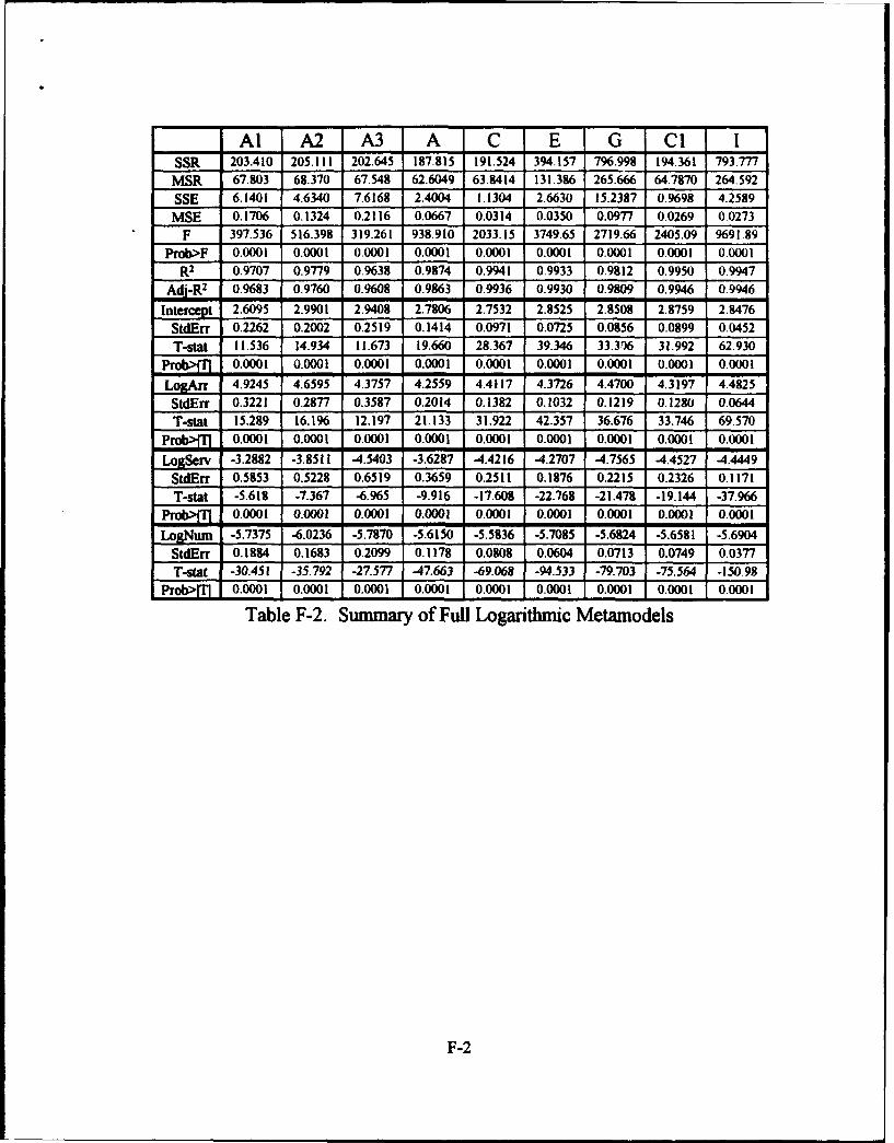
Al A2 A3 A C E G CI ISSR 203.410 205.111 202.645 187.815 191.524 394.157 796.998 194.361 793.777MSR 67.803 68.370 67.548 62.6049 63.8414 131.386 265.666 64.7870 264.592

SSE 6.1401 4.6340 7.6168 2.4004 1.1304 2.6630 15.2387 0.9698 4.2589

MSE 0.1706 0.1324 0.2116 0.0667 0.0314 0.0350 0.0977 0.0269 0.0273

F 397.536 516.398 319.261 938.910 2033.15 3749.65 2719.66 2405.09 9691.89

Prob>F 0.0001 0.0001 0.0001 0.0001 0.0001 0.0001 0.0001 0.0001 0.0001R2 0.9707 0.9779 0.9638 0.9874 0.9941 0.9933 0.9812 0.9950 0.9947

Adj-R2 0.9683 0.9760 0.9608 0.9863 0.9936 0.9930 0.9809 0.9946 0.9946

Intercept 2.6095 2.9901 2.9408 2.7806 2.7532 2.8525 2.8508 2.8759 2.8476StdErr 0.2262 0.2002 0.2519 0.1414 0.0971 0.0725 0.0856 0.0899 0.0452

T-stat 11.536 14.934 11.673 19.660 28.367 39.346 33.316 31.992 62.930Prob>M 0.0001 0.0001 0.0001 0.0001 0.0001 0.0001 0.0001 0.0001 0.0001

LogArr 4.9245 4.6595 4.3757 4.2559 4.4117 4.3726 4.4700 4.3197 4.4825StdErr 0.3221 0.2877 0.3587 0.2014 0.1382 0.1032 0.1219 0.1280 0.0644

T-stat 15.289 16.196 12.197 21.133 31.922 42.357 36.676 33.746 69.570

Prob>M 0.0001 0.0001 0.0001 0.0001 0.0001 0.0001 0.0001 0.0001 0.0001

LogServ -3.2882 -3.8511 -4.5403 -3.6287 4.4216 4.2707 4.7565 4.4527 4.4449StdErr 0.5853 0.5228 0.6519 0.3659 0.2511 0.1876 0.2215 0.2326 0.1171T-stat -5.618 -7.367 -6.965 -9.916 -17.608 -22.768 -21.478 -19.144 -37.966

Prob>M 0.0001 0.0001 0.0001 0.0001 0.0001 0.0001 0.0001 0.0001 0.0001

LogNum -5.7375 -6.0236 -5.7870 -5.6150 -5.5836 -5.7085 -5.6824 -5.6581 -5.6904StdErr 0.1884 0.1683 0.2099 0.1178 0.0808 0.0604 0.0713 0.0749 0.0377T-star -30.451 -35.792 -27.577 47.663 -69.068 -94.533 -79.703 -75.564 -150.98

Prob>m 0.0001 0.0001 0.0001 0.0001 0.0001 0.0001 0.0001 0.0001 0.0001Table F-2. Summary of Full Logarithmic Metamodels

F-2

A- A2 A3 A C E G CI ISSR 10.1505 14.1378 11.3631 12.6599 11.2027 25.3662 53.1240 12.7340 53.0610

MSR 3.3835 4.7126 3.7877 4.2200 3.7342 8.4554 17.7080 4.2447 17.6870SSE 0.6105 0.9375 0.6582 0.4895 0.0877 0.5504 2.6030 0.0024 0.4116MSE 0.03815 0.0586 0.0411 0.0306 0.0055 0.0153 0.0343 0.0001 0.0054

F 88.681 80.432 92.07 137.923 681.077 553.014 517.010 28185.1 326582

Prob>F 0.0001 0.0001 0.0001 0.0001 0.0001 0.0001 0.0001 0.0001 0.0001

R2 0.9433 0.9378 0.9452 0.9628 0.9922 0.9788 0.9533 0.9998 0.9923Adj-R2 0.9326 0.9262 0.9350 0.9558 0.9908 0.9770 0.9514 0.9998 0.9920

Intercept 3.3212 3.937 3.5666 3.7322 3.5172 3.7394 3.8234 3.7544 3.8231StdEff 0.4704 0.5829 0.4885 0.4213 0.1783 0.2106 0.2229 0.0296 0.0886T-stat 7.060 6.754 7.301 8.860 19.723 17.758 17.157 127.032 43.142

Prob> 0.0371 0.0001 0.0001 0.0001 0.0001 0.0001 0.0001 0.0001 0.0001

Ar 1.5624 1.853 1.6366 1.7472 1.6414 1.7512 1.7977 1.7450 1.7929StdErr 0.1747 0.2165 0.1814 0.1565 0.0662 0.0782 0.0828 0.01 10 0.0329T-stt 8.943 8.559 9.021 11.168 24.784 22.393 21.720 158.978 54.475

Prob>M 0.0001 0.0001 0.0001 0.0001 0.0001 0.0001 0.0001 0.0001 0.0001Serv -3.0464 -3.6564 -3.2524 -3.448 -3.2452 -3.4656 -3.557 -3.4524 -3.5473StdEfrr 0.3494 0.4330 0.3628 0.3129 0.1325 0.1564 0.1655 0.0220 0.0658T-stat -8.719 -8.444 -8.964 -11.019 -24.500 -22.157 -21.488 -157.27 -53.892

Prob>T 0.0001 0.0001 0.0001 0.0001 0.0001 0.0001 0.0001 0.0001 0.0001

Num -0.4582 -0.5324 -0.4853 -0.5064 -0.4767 -0.5048 -0,5141 -0.5101 -0.5155StdErr 0.0437 0.0541 0.0454 0.0391 0.0166 0.0196 0.0207 0.0027 0.0082T-stat -10.491 -9.835 -10.699 -12.947 -28.788 -25.820 -24.850 -185 87 -62.655

Prob>m 0.oo1 0.0001 0.0001 0.0001 o0.0001 oo0.0001 0.000o 00001 000Table F-3. Summary of Fractional Linear Metamodels

F-3

k II I I II II I I

Al A2 A3 A C E G CI ISSR 100.456 113.160 92.1069 100.005 93.7513 201.050 377.018 96.1377 387.412

MSR 33.4853 37.7200 30.7023 33.3352 31.2504 67.017 125.673 32.0459 129.138

SSE 1.6747 2.5417 3.9095 1.3235 0.3778 1.0320 5.3466 0.1528 1.0106

MSE 0.1047 0.1587 0.2444 0.0827 0.0236 0.0287 0.0704 0.0096 0.0133

F 319.917 237.445 125.651 402.993 1323.40 2337,90 1786.42 3354.88 9711.48

Prob>F 0.0001 0.0001 0.0001 0.0001 0.0001 0.0001 0.0001 0.0001 0.0001R2 0.9836 0,9780 0.9593 0.9869 0.9977 0.9949 0.9860 0.9984 0.9974

Adj-R2 0.9805 0.9739 0.9516 0.9845 0.9973 0.9945 0.9855 0.9981 0.9973

Intercept 2.4580 3.0155 2.9991 2.8610 2.7986 2.9286 2.8400 2.9572 2.8937

StdErr 0.2506 0.3087 0.3829 0.2228 0.1190 0.0927 0.1027 0.0757 0.0447

T-stat 9.809 9.767 7.833 12.842 23.511 31.580 27.647 39.063 64.791

Prob>M 0.0001 0.0001 0.0001 0.0001 0.0001 0.0001 0.0001 0.0001 0.0001

LogAfr 5.0183 4.8147 3.6789 4.4387 4.1546 4.3208 4.1948 4.1041 4.2587

StdErr 0.3568 0.4396 0.5452 0.3172 0.1695 0.1320 0.1463 0.1078 0.0636

T-stat 14.063 10.952 -4.042 13.992 24.513 32.722 28.678 38.072 66.967

Prob.M 0.0001 0.0001 0.0009 0.0001 0.0001 0.0001 0.0001 0.0001 0.0001

LogServ -1.4468 -2.6175 -4.0048 -3.0622 -3.5630 -3.5426 -3.9288 -3.5265 -3.6884StdErr 0.6484 0.7988 0.9907 0.5764 0.3080 0.2399 0.2658 0.1959 0.1156

T-stat -2.231 -3.277 -4.042 -5.312 -11.569 -14.765 t 4.782 -18.004 -31.920

Prob>ITI 0.0403 0.0047 0.0009 0.0001 0.0001 0.0001 0.0001 0.0001 0.0001

LogNum -5.7431 -6.2019 -5.6611 -5.8238 -5.6395 -5.8444 -5.6227 -5.7417 -57185StdErr 0.2087 0.2572 0.3189 0 1856 0.0991 0.0772 0.0856 0.0661 0.0372T-stat -27.514 -24.117 -17.750 -31.384 -56.881 -75.664 -65.714 -91.055 -153.72

Prob>ITI 0.0001 0.0001 0.0001 0.0001 0.0001 0.0001 0.0001 0.0001 0.0001Table F-4. Summary of Fractional Logarithmic Metamodels

F-4

Bibliography

Barton, Russell R. "Metamodels for Simulation Input-Output Relations," Proceedings ofthe 1992 Winter Simulation Conference. 289-299. New York: IEEE Press,1992.

Box, George E. P., and Norman R. Draper. Empirical Model-Building and ResponseSurfaces. New York: John Wiley and Sons, 1987.

Donovan, James L. An Application of Response Surface Methodology to aMacroeconomic Model. MS Thesis, AFIT/GORJENS/85D-5. School ofEngineering, Air Force Institute of Technology (AU), Wright-Patterson AFB OH,December 1985.

Draper, Norman R., and Harry Smith. Applied Regression Analysis (Second Edition).New York: John Wiley and Sons, 1981.

Friedman, Linda Weiser, and Friedman, Hershey H. "Validating the SimulationMetamodel: Some Practical Approaches," Simulation. Vol 45, Issue 3: 144-146(September 1985).

Goldsman, David. "Simulation Output Analysis," Proceedings of the 1992 WinterSimulation Conference. 97-103. New York: IEEE Press, 1992.

Harvey, R. Garrison, and others. "Force Allocation Through Constrained Optimization ofStochastic Response Surfaces," Proceedings of the 1992 Winter SimulationConference. 1121-1129. New York: IEEE Press, 1992.

Jobson, J. D. Applied Multivariate Data Analysis. Volume I: Regression andExperimental Design. New York: Springer and Verlag, 1991.

Khuri, Andre I., and John A. Cornell. Response Surfaces. New York: MarcelDekker, Inc., 1987.

Kleijnen, Jack P. C. Statistical Tools for Simulation Practitioners. New York: MarcelDekker, Inc., 1987.

Kleijnen, Jack P. C. and others. Techniques for Sensitivity Analysis of SimulationModels: A Case Study of the CO Greenhouse Effect. Tilburg, The Netherlands:Tilburg University, June 1990 (AD-B 156-767).

Bib-I

Law, Averill M. and W. David Kelton. Simulation Modeling & Analysis (SecondEdition). New York: McGraw-Hill, Inc., 1991.

Mendenhall, William and others. Mathematical Statistics with Applications (FourthEdition). Boston: PWS-Kent, 1990.

Montgomery, Douglas C. Design and Analysis of Experiments (Third Edition). NewYork: Wiley and Sons, 1991.

Nelson, Barry L. "Designing Efficient Simulation Experiments," Proceedings of the 1992Winter Simulation Conference. 126-132. New York: IEEE Press, 1992.

Neter, John and others. Applied Linear Statistical Models (Third Edition). Boston:Irwin, 1990.

Palasota, John A. and Stanley N. Deming. "Central Composite Designs Applied toChemical Systems," Journal of Chemical Education. Volume 69. Number 7: 560-563 (July 1992).

Pritsker, A. Alan B. Introduction to Simulation and SLAM U (Third Edition).New York: Wiley, 1986.

Ross, Sheldon M. Introduction to Probabiiby Models (Fourth Edition). New York:Academic Press, Inc., 1989.

Sargent, Robert G. "Research Issues in Metamodefing," Proceedings of the 1992 WinterSimulation Conference. 887-893. New York: IEEE Press, 1992.

Shannon, Robert E. "Introduction to Simulation," Proceedings of the 1992 WinterSimulation Conference. 65-73. New York: IEEE Press, 1992.

Turban, Efraim and Jack R. Meredith. Fundamentals of Management Science (FifthEdition). Boston: Irwin, 1991.

Whitt, Ward. "The Efficiency of One Long Run Versus Independent Replications inSteady-State Simulation," Management Science. Vol 37, Issue 6: 645-666(June 1991).

Yielding, Gary E. Automating Response Surface Methodology for the Arsenal ExchangeModel. MS Thesis, AFIT/GOR/ENS/86D- 17. School of Engineering, Air ForceInstitute of Technology (AU), Wright-Patterson AFB OH, May 1987.

Bib-2

Vita

Captain Michael Kent Taylor was born on March 3, 1964 in Fort Walton Beach,

Florida. He graduated from Choctawhatchee High School in Fort Walton Beach in 1982

and attended the University of Alabama at Birmingham, graduating with a Bachelor of

Science Degree in Mathematics in June 1986. Upon graduation he received a reserve

commission in the USAF and served his first tour of duty at Eglin AFB, Florida in October

1986. He began as a Tactical Command, Control, and Communications Countermeasures

Operations Analyst for the Tactical Air Warfare Center where he supported the

Operational Test and Evaluation of the Compass Call Airborne Jammer until August 1989.

He then was selected for assignment to Headquarters, Tactical Air Command,

DCS/Requirements at Langley AFB, Virginia where he was a Command, Control,

Communications, and Intelligence (C31) Operations Analyst assigned to the Directorate of

Battle Management. In that position, he was responsible for the interoperability of C31

and weapons platforms via digital data links of the USAF, US, NATO, and allies until

entering the School of Engineering, Air Force Institute of Technology (AFIT), in August

1992. In June 1993, he received his regular commission. Upon completion of his studies

at AFIT, he was selected for assignment to the Air Force Studies and Analyses Agency in

the Force Applications Directorate as a Theater Command and Control Analyst in the

Theater Air Defense Division, DSN 225-5282.

Permanent Address: 120 Boyce DriveShahimar FL 32579

V-I

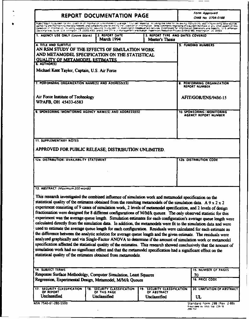
REPORT DOCUMENTATION PAGE I F0o1rN.07m08

* P~1"40.c eocrv' ,g -~''if It~s z'emcn~ ot #0-at'an, 'S e I-'w & .e'&C, :-.1 Der 'f1wo"se nc'LdIotlng M .e t. 01'fte.ewnq 1Str-.t,.1.S ýear:',ng exug cata sources,,ah~ nd a1" b~- the cats ne~eaC. an* comme.ting ana e ý@-n ," :'.. c "0 "'C~O "' normgt.to Sena comnmentj reqa'.vtq C~lIngM1 b..ddert eit-ate C,, an# 3tI'Cf &WC~t Ot INSl

colleco' -fnc'r''a, "''~ sugetto % lot 'eoucing In%0,re to ..'e a,1-910" -'eaaaua!er Selý,Ces_ Drectofateto 'nlor'r.aror oe'at.or', ana Rego',. ! 2IS 'etferwrDa.I.S gr~ar it '24 ' on . *a 22202I4302 ana o tO 0*O -,e ), %Aa de"'Cnt and8..udge' P4Pe`I"0f Reducti0m Project (0704-0'S8). AehoVngton D'C 20S03

1. AGENCY USE ONLY (Leave bIn)I2. REPORT DATE I3. REPORT TYPE AND DATES COVERED

77 Mach 199 Mastcers Thesis4. TITLE AND SUBTITLE 5. FUNDING NUMBERSAN RSM STUDY OF THE EFFECTS OF SIMULATION WORKAND METAMODEL SPECIFICATION ON THE STATISTICALOUALITY OF MTOELESTIMATES6. AUTHOR(S)

Michael Kent Taylor, Captain U.S. Air Force

7. PERFORMING ORGANIZATION NAME(S) AND ADDRESS(ES) B. PERFORMING ORGANIZATIONREPORT NUMBER

Air Force Institute of Technology AFI/GOR/ENS/94M- ISWPAFB, OH 45433-6583

9. SPONSORING/ MONITORING AGENCY NAME(S) AND ADDRESS(ES) 10. SPONSORING / MONITORINGAGENCY REPORT NUMBER

11. SUPPLEMENTARY NOTES

APPROVED FOR PUBLIC RELEASE; DISTRIBUTION UNLIMITED.

12a. DISTRIBUTION Y AVAILABILITY STATEMENT [12b. DISTRIBUTION CODE

13. ABSTRACT (Maximum 200 words)

This research investigated the combined influenice of simulation work and metazuodel specification on thestatistical quality of the estimates obtained from the resulting metamodels of the simulation data. A 9 x 2 x 2experiment consisting of 9 cases of simulation work, 2 levels of metamodel specification, and 2 levels of designfractionation were designed for 8 different configurations of M/NI/k queues. The only observed statistic for thisexperiment was the average queue length. Simulation estimates for each configuration's average queue length were

cacltddirectly from the simulation data. In addition, the metamodels were fit to the simulation data and wereused to estimate the average queue length for each configuration. Residuals were calculated for each estimate asthe difference between the analytic solution for average queue length and the given estimate. The residuals wereanalyzed graphically and via Single-Factor ANOVA to determine if the amount of simulation work or metamodelspecification affecte the statistical quality of the estimates. This research showed conclusively that the amount ofsimulation work had no significant effect and that the metamodel specification had a significant effect on thestatistical quality of the estimates obtained from metamodels.

14. SUBJECT TERMS 15. NUMBER OF PAGESResponse Surfakce Methodolgy, Computer Simulation, Least Squares 70Regression, Expermental Design, Metamodel, M/NI/k Queues 16. PRICE CODE

17. SECURITY CLASSIFICATION 18. SECURITY CLASSIFICATION 19. SECURITY CLASSIFICATION 20. LIMITATION OF ABSTRACTOF REPORT OF THIS PAGE OF ABSTRACT

Unclassified Unclassified Unclassified ULNSN 7540-01-280-5500 Stan~dard ;orm 298 (Rev 2-89)

Oe .c o 0 :..Si Sto Z39'S8

afit/gor/ens/94m- 15 · today's air force. his contributions to this research and my career...

Documents