aerothermal analysis and characterization of shielded fine

XXI Biannual Symposium on Measuring Techniques in Turbomachinery

Aerothermal Analysis and Characterization of Shielded Fine WireThermocouple Probes

Laura Villafane, Guillermo Paniagua

Turbomachinery and Propulsion Departmentvon Karman Institute for Fluid Dynamics

Chaussee de Waterloo 72Rhode-Saint-Genese, 1640, Belgium

Email: [email protected]

Abstract

Thermocouple probes for high accuracy gas temperature measurements require specific designs optimized forthe application of interest and precise characterization of the uncertainty. In the present investigation a numericalprocedure is proposed that outperforms previous experimental approaches to analyze the thermocouple responseand the different sources of temperature error. The results presented from conjugate heat transfer simulations ondifferent shielded thermocouples provide information of the influence of the design parameters on the differenterror sources. These outcomes could help experimentalists to better design future instrumentation.

Keywords: thermocouples, conjugate heat transfer (CHT), recovery factor, conduction effects, response time,transfer function

1. Introduction

In transonic intake research [1] high fidelity in the total temperature is needed. In the present investigationnumerical simulations were performed to study the steady and unsteady heat fluxes within a temperature probe toevaluate both the temperature during a transient and at equilibrium.

Multiple attempts to provide correction factors for standard thermocouple designs were found in the literature[2],[3],[4]. Traditionally over-all recovery factors were experimentally determined as an indicator of the tempera-ture error of a thermocouple. Such global recovery factors accounted for the total effect of radiation, conductionand convection on the probe for a given flow environment. The variability of the heat fluxes balance within theprobe with the environment and probe design, required each thermocouple to be carefully designed and calibratedfor the required application. However, precise corrections from experimental probe calibrations are impractical.During such calibration not only the flow conditions need to be replicated but also the thermal interactions bet-ween the probe and the test bench. Furthermore, the precision to reproduce and to characterize the calibrationenvironment determines the accuracy of the corrections.

The numerical characterization of the probes excelled previous experimental experiences in accuracy. Thepresented numerical methodology allowed understanding and quantifying the effects of the design parameters, re-quired to achieve precise gas temperature measurements. Adiabatic recovery factors, conduction error estimationsand response time characteristics were determined for a shielded probe with different values of thermocouple wirediameter, wire materials and boundary conditions at the thermocouple wire support. The presented numericalapproach may be coupled with optimizers to design the best probe for any specific application.

2. Thermocouple Probe Design

2.1. Application

A transonic wind tunnel with a distorted annular sector, helicoidal test section was manufactured to study anovel heat exchanger [1]. Total flow temperature measurements were to be performed in this intermittent windtunnel discharging to the atmosphere from a pressurized vessel. The flow temperature decreased during a test run

1 ValenciaMarch 22-23, 2012


due to the flow expansion in the reservoir. Flow temperature traverses were to be recorded along the test section ofabout 0.013 m2 transversal area. High-frequency response was required in order to allow fast traverses. A rake oftemperature probes allowed to maximize the measurement locations in a test. Precise characterization of the proberesponse was necessary to synchronize all readings, as well as to accurately analyze the heat exchanger efficiency.

2.2. Pre-existent design rules

The temperature of a thermocouple junction is the result of the energy balances including the convective heatflux between the junction and the surrounding gas, radiation to the walls, and conductive flux to the wire. Thebalance is different for each probe and each condition. The measured temperature would be equal to the total flowgas temperature in the absence of radiative heat fluxes, conductive flux to the thermocouple support and dissipationof kinetic energy in the boundary layer.

General design rules provide advises to reduce the temperature error sources. A shield is recommended inorder to decrease the error caused by the dissipation of kinetic energy in the boundary layer around the junction(often called velocity error). The shield also provides structural resistance in high velocity flows and reducesradiation effects. However decreasing the velocity of the flow decreases the convective heat transfer, penalizing theconduction error and the response time. Thus, the internal velocity must be kept as high as allowable. The internalvelocity is function of the vent hole to inlet ratio. The junction position within the shield is a compromise betweennon-aligned entrance flow effects, and flow alteration due to convective heat transfer to the shield. Recommendedvalues are given by Rom and Kronzon [3], Saravanamuttoo [5] and Glawe et al. [2]. The wires within the shieldcan be placed parallel or perpendicular to the flow. In the first case, the length of the wires is limited to preventwire bending. In the second, the length is limited by the shield diameter.

Conduction errors can be estimated from the simplified solution of the 1D energy equation for a wire elementdx, (Eq.1), considering symmetry boundary condition ∂T/∂x = 0 at the junction (x = 0), and isothermal tem-perature Tw = Tsp at the support of the wire (x = l). Eq. 2 provides a simplified solution particularized for thejunction. The assumption of constant gas temperature and constant convection coefficient h, neglects the effect ofthe real flow temperature differences along the wire.

h(T − Tg)πdwdx = k∂2T∂x2 π

d2w

4dx (1)

Tad − T j =Tad − Tsp

cosh(l√

4hkwdw

)=

Tad − Tsp

cosh(l/lc)(2)

Let us consider the total temperature of the gas Tg, equal to the junction recovery temperature Tad, namely thetotal temperature in the absence of velocity error. Design rules derived from this simplified solution recommend tohave high values of h (high velocities), high l/dw ratios, low conductivity wire materials, and support temperaturesclose to gas temperature. Petit et al. [6] suggest that the ratio l/lc should not be smaller than 5.

The contribution of the error due to radiation is generally important at high flow temperatures The simplifiedrelationship (Eq.3) considering the most adverse conditions with unity view factor and equal conductive andradiative areas yielded a negligible error, lower than 4 · 10−4%, about 1 mK.

T0 − T j =KRσεAR(T 4

j − T 4W )

hAc(3)

In flow temperature transients the energy balance at the thermocouple junction or on a dx at any position alongthe wire can be expressed by Eqs. 4. As in the steady case, Tg is considered equal to Tad in the absence of velocityerrors.

S jh j(Tg − T j) +π

2d2

wkw(∂2Tw

∂x2 )|x=0 = ρ jCp, jV j∂T j

∂t

hw(Tg − Tw) +dw

4kw(

∂2Tw

∂x2 ) = ρwCp,wdw

4∂Tw

∂t

(4)



Side

cross-section

Front view

Figure 1: Shielded thermocouple probe.

In the case of uniform temperature on the junction, constant heat transfer coefficient independent with time,and no heat transfer by conduction between the junction and the adjacent wire, the thermocouple response to atemperature step is a first order system, Eq. 5. The assumption of first order system would be also valid forthe assembly wire and junction if their diameters are identical, there are no radial or longitudinal temperaturegradients, no conductive heat transfer to the supports, and the heat transfer coefficient is constant in time andalong the length of the wire. Eq. 5, provides the time constant.

Tg = T j + τ∂T j

∂t, with τ j =

ρ jCp j V j

h jS j; τw =

ρwCpw d2w

4kgNuw(5)

2.3. Shielded probe design

The temperature probe consists of a rake of five shielded thermocouples. Minimization of blockage effectsgiven the small transversal area of the test section is considered, while preserving the structural resistivity of thewhole rake. The geometric characteristics of the temperature probe heads are sketched in Fig. 1.

A type T thermocouple (copper-constantan) is placed perpendicular to the flow with a total length equal tothe internal shield diameter, 2 mm. This wire configuration is intended to avoid wire bending at high velocities.Ratios (l/d)w of 79 are obtained with wires of 25.4 µ m diameter. The ratio weld-bead to wire diameter measuredafter probe manufacturing is about 2.7. The shield diameter is a compromise between the blockage minimization,wire structural resistivity and limitation of conduction errors. The shield is made of polycarbonate, chosen for itslow conductivity. In agreement with the values recommended in the literature [2], [3], [5], the inlet/outlet arearatio is 4 and the junction is placed at 1/2 internal shield diameters from the entrance.

3. Methodology of the aerothermal study.

The transfer function of the thermocouple probe was numerically obtained by evaluating the response to atemperature step. Experimentally, the accuracy of the temperature corrections required a precise control of the gastemperature excitation and test conditions.

At the transonic conditions of interest, the characteristic time for the flow to develop around the thermocoupleis two orders of magnitude smaller than the characteristic time of the thermal transient in the thermocouple wires.This allows performing simulations in two stages. First, a steady simulation is solved to establish the flow aroundthe probe considered isothermal. The flow-field solution of this first step is imposed as initial condition for thesimulation of the second step. In the second step, the solid boundary conditions are changed and a conjugate heattransfer (CHT) simulation is performed, solving the energy balances within the thermocouple. This second stageis ran in steady or transient state depending on whether the interest is focused on the steady temperature errors oron the transient behavior. In the latter case, the result is the response of the thermocouple to a temperature step.The decomposition in two stages highly reduces the computational cost.

This methodology allows the detailed analysis of the heat fluxes within the thermocouple probe, and theevaluation of the influence of the flow environment, probe geometry and wire materials.



Figure 2: Computational domain. Left: TC shield view. Right: TC wire and junction.

Table 1: Probe geometric configurations.

Geom 1 Geom 2 Geom 3l, [mm] 1 1 1

dw, [mm] 0.0254 0.0508 0d j, [mm] 0.07 0.14 0.07

4. Numerical Tools.

4.1. Computational domain and solver

The shielded thermocouple head is modeled in a 3D domain constituted by a quarter of a cylinder thanks tothe existence of two symmetry planes on the probe geometry. The grid extends 6 shield diameters in the radialdirection and in the axial direction upstream of the probe, and 10 diameters downstream. The three solid parts(shield, wire and junction) are meshed independently and concatenated to the gas domain mesh in the used NSsolver. The gas hybrid 3D mesh composed by about 1.75 million cells is shown in Fig. 2-b. The grid is refinedalong the walls of the solid parts and specially around the thermocouple wire and junction (Fig. 2-c).

The Reynolds Averaged Navier Stokes solver employed was CFD++ (v.8.1). The k-epsilon turbulence modelwas considered. The initial values of k and epsilon were estimated in function of the free stream nominal velocity,with a free-stream turbulence level of 1% and a turbulence length scale based on the tube inner diameter. Values ofy+ in the vicinity of the thermocouple junction are lower than 0.3, and lower than 0.5 along the wire. For the steadysimulations on both stages, convergence was achieved after 1000 iterations , 5.5 hours CPU time in 8 parallel IntelCore 2 Quad Q9400 (2.66 GHz) machines. For the transient CHT simulations the number of iterations requiredto achieved convergence varied depending on the wire material simulated. As an average 1000 iterations withdifferent time steps were required, involving 51 hours CPU time running in 8 parallel machines. The integrationtime step was adjusted as function of the rate of evolution of the junction temperature, starting from 0.1ms.

4.2. Numerical test conditions

Nominal flow conditions for the simulations correspond to inlet boundary conditions Ts = 273.22K, Ps =

101325Pa, V∞ = 231.12m/s, and Ps = 101325Pa at the domain outlet. Different Mach and Reynolds numberswere tested for the geometrical configuration corresponding to the design geometry, Table??.

Three geometrical configurations were analyzed: Geom 1,2 and 3, (ref. 1). The shield is the same in the threecases. Geom 1 corresponds to the design geometry. The modified parameter is the wire diameter, doubled in Geom2 where the ratio junction to wire diameter has been kept constant. Geom 3 refers to the test case of a junctionwith infinitely thin wires.



Heat loss through the wires to the support is function of the wire dimensions and flow conditions (convection),but also of the material conductivity, and the support temperature. Different wire materials and boundary condi-tions at the support were analyzed for the configurations Geom 1 and Geom 2. In all cases the shield material ispolycarbonate and the junction properties are the average of the two materials of type T thermocouple. Other twomaterials of lower conductivity were considered: Nicrosil and an ideal material with conductivity equal to one,Tab. 2. The different support boundary conditions tested were:

(a) The shield-support behaves as an adiabatic solid,(b) the shield is isothermal at 300 K,(c) CHT on the shield.

Table 2: Material properties of thermocouple wires. Evaluated at 23◦C.

Copper Constantan Nicrosil Ideal PolycarbonateK, [W m-1 K-1] 401 19.5 13 1 0.2ρ, [kg m-3] 8930 8860 8530 8860 1210Cp, [J kg-1 K-1] 385 390 460 390 1250

5. Steady Temperature Effects

5.1. Global Temperature CorrectionThe junction temperature results from the balance between the convective heat fluxes gas-junction and gas-

wire, and conductive flux junction-wire and wire-support. If those effects were decoupled, individual error equa-tions could be used to estimate the deviation of the measured temperature. However, in practical applications thejunction temperature must be evaluated by the simultaneous solution of the different heat flux rates [7].

The overall recovery factor Z (Eq. 6),the difference between the measured temperature (T j) and the total gastemperature (T0), can be decomposed into several contributions. The first term (a) is the velocity error, related tothe adiabatic recovery factor. The second term (b), takes into account the temperature error due to conduction andconvection along the wire, for a given support-shield temperature, (Tsp). The last term (c) collects the velocityerror of the support-shield and the conduction effects between the shield, probe stem, and external probe support.The numerical method applied allows analyzing separately each contribution.

(1 − Z) =T0 − T j

T0 − T∞=

a︷︸︸︷T0 − Tad

T0 − T∞+

b︷︸︸︷Tad − T j

Tad − Tsp·

c︷︸︸︷Tad − Tsp

T0 − T∞(6)

5.2. Velocity errorTemperature probes are intended to measure the gas total temperature, i.e. the temperature that the gas would

attain if it is brought to rest through an isentropic process. However, in real gases frictional heat is generated withinthe boundary layer, hence the conversion of kinetic energy into thermal enthalpy is not perfect. The recovery factor,Eq. 7, represents the amount of kinetic energy recovered by the gas, where Tad is the temperature of the surface ofthe junction if it would behave as an adiabatic body, and V is the reference upstream flow velocity. The recoveryfactor is function of the geometry of the immersed body and the Prandtl number of the fluid. Experimental valuesof adiabatic recovery factor determined by different authors [8],[9],[10] were presenteed by Moffat [11].

r =Tad − Ts

V2/2Cp= 1 −

T0 − Tad

V2/2Cp(7)

For shielded thermocouples behaving as adiabatic bodies, the term (a) in Eq. 6 represents an overall adiabaticrecovery factor, related to r by Eq.8. The velocity upstream of the junction within the shield(V) is different fromthe free stream flow velocity(V∞).



Za =Tad − Ts

V2∞/2Cp

= 1 −T0 − Tad

V2∞/2Cp

= 1 − (1 − r)V2

int

V2∞

(8)

Experimental determination of recovery factors was impractical since the junction temperature has to be de-termined with great accuracy, and ensuring negligible influence of conduction to the supports, so the junctionbehaves as an adiabatic body. Steady simulations at different flow velocities allowed determining both r and Za

and their sensibility to flow Mach and Reynolds numbers. Wire and shield were considered adiabatic solids in thecomputations and CHT was solved at the junction, at Tad.

Computations were also performed considering all the solid boundaries adiabatic, junction included. Theaverage temperature on the junction adiabatic surface Tad,m was compared with the junction temperature obtainedwhen CHT was applied. Temperature differences were observed to be lower than 0.004 % (Tad,m − Tad/Tad,m).These small differences were explained by the junction heat capacity.

0 . 4 0 . 6 0 . 80 . 4

0 . 6

0 . 8

1 . 0

0 . 4

0 . 6

0 . 8

1 . 0

R e = 1 9 1 R e = 3 8 3 G e o m 1 R e = 4 5 9 R e = 7 6 5 G e o m 2 R e = 3 8 3 G e o m 3

Z ar

M

0 7.06 8.0 ±

M o f f a t , 1 9 6 1

0 . 4 0 . 6 0 . 80 . 0 2

0 . 0 4

0 . 0 6

0 . 0 8

R e = 3 8 3

(T 0-T ad)/T

0

M

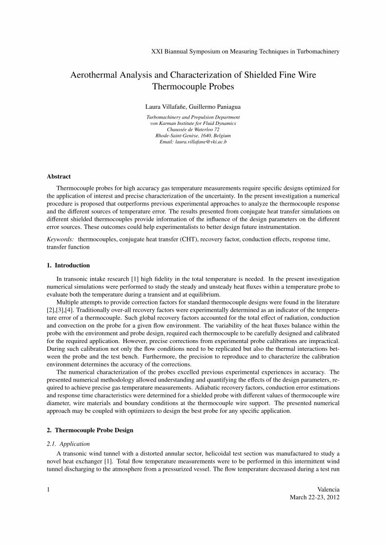
Figure 3: a) Recovery factors for different probe geometries, Mach and Reynolds numbers, b) Temperature error due to no isentropic flowdeceleration

Figure 3(a) shows the evolution of the recovery factor (r), and the overall recovery factor (Za), for differentReynolds and Mach numbers. The adiabatic recovery factor slightly increases with the flow Mach number, andthus with the velocity within the shield (about six times slower than the external flow). The results are in goodagreement with the recovery values compiled by Moffat [11]. For the same probe geometry Geom 1, at constanttemperature and Mach number, an increase in the Reynolds number achieved through an increase in static pressure,results in a slightly decrease of the recovery factor. An increase of the Reynolds number at nominal flow conditionsdue to the increase of the wire and junction diameter (Geom 2), yields to an analogous decrease of the recoveryfactor. The overall recovery factor shows the same trend but less sensitive to Mach and Reynolds variations.

Recovery factors were computed likewise for Geom 3, providing lower values. The flow behavior arounda sphere is not similar to that around a thermocouple junction, neither to the flow parallel to a cylinder [11].Comparison of the flow fields around the junction for Geom 1 and Geom 3, showed a stronger flow decelerationin the first case forced by the presence of the wires, and hence, a thicker thermal boundary layer. Consequentlythe transformation of the flow kinetic energy into thermal energy is more efficient.

Although the recovery factor increases with the Mach number, the kinetic velocity rises in a higher amount,thus the temperature error represented in Fig. 3(b) also increases with velocity.

5.3. Conduction error

Free of velocity errors, the difference between the real junction temperature and the total temperature is theerror due to conduction, namely the product of terms (b) and (c) in Eq.6. In a well designed thermocouple thejunction temperature should be little sensitive to the support temperature, i.e. the term (b) is close to zero. Inthat case the overall contribution of conduction would be negligible whatever is the value of term (c). In realapplications term (b) is different to zero.



0 1 0 2 0 3 0 4 00 . 0

0 . 4

0 . 8

k = 1

C o n s t a n t a n

N i c r o s i lk e q

C o p p e r

C o n s t a n t a n

C o p p e r

y = 1 . 5 ( l / l c ) - 1 . 2

G e o m 1 ( l / d w = 7 9 ) G e o m 2 ( l / d w = 3 9 . 5 ) A n a l y t i c a l s o l u t i o n

(T ad-T j)/(T

ad-T sp

)

l / l c

y = 1 . 1 ( l / l c ) - 1 . 2

y = c o s h - 1 ( l / l c )

Figure 4: Ratio junction to support temperature deviations with respect to total temperature in function of the parameter l/lc. Results fromCHT simulations

Term (b) reflects the influence on the junction of the balance conduction-convection along the wire and theconduction with the support. Its contribution can be estimated by the solution of the one dimensional energyequation, Eq.2, that predicts an exponential decrease with the increase of the parameter l/lc (for x≥ 5, cosh x '0.5ex). Term (c) indicates the strength of the conduction heat transfer between the thermocouple and the support.The lower temperature of the shield-support with respect to the total gas temperature (Tad in the absence of velocityerror), Tad−Tsp, drives the conduction to the wire. In the case the support would be perfectly isolated from externalsources, it is function of the recovery factor of the complete shield/support. In real applications it is also functionof the depth of immersion of the support in the flow, the support geometry and thermal properties, and the externalboundary conditions of the probe.

The values of the parameter l/lc for each material and the geometries Geom 1 and 2 are indicated in Tab. 3.For the computation of l/lc, Eq. 9, air conductivity is evaluated at the gas total temperature [7], and the Nusseltnumber is derived from a correlation for wires perpendicular to the flow [11]: Nu = (0.44 ± 0.06)Re0.5.

llc

= l

√4h

kwdw=

2ldw

√Nukg

kw(9)

Table 3: Material parameters of thermocouple wires affecting conduction.Constantan Copper Nicrosil Ideal Equivalent

k, [kW m-1 K-1] 19.5 401 13 1 6.89l/lc (Geom 1) 8.43 1.86 10.33 37.24l/lc (Geom 2) 5.01 1.11 n.a. n.a. 8.43

Fig. 4 shows the non-dimensional conduction temperature error corresponding to term(b) in Eq.6. All resultscorrespond to complete CHT simulations. The temperatures difference ratio is plotted versus the parameter l/lc,which for a given probe geometry is only varied by a change in the wire material. The error decreases as theparameter l/lc increases indicating that the junction temperature is less influenced by the conduction effects. Theresults show two slightly distinct trends for each l/dw case that are best fitted by power laws with a common expo-nent coefficient of -1.2. The equivalent material, keq, corresponds to an hypothetical material with a conductivitysuch that the l/lc value for Geom2 is equal to the l/lc value for constantan wire and Geom1 (keq = kconst

√2/4).

At this l/lc value (8.43), the contribution of conduction of term (b) is slightly smaller for Geom2. The analyticalprediction (Eq.2) underestimates the results when compared with the numerical results. This discrepancy can beexplained by the simplifications introduced in the analytical solution, especially the assumption of homogeneousgas temperature and heat transfer coefficient along the wire, and equal to the conditions and geometry at the junc-tion. The parameter l/lc is a good estimator of the conduction error, but inappropriate to establish a unique relation



with the temperature error.

0 1 0 2 0 3 0 4 00 . 0 0

0 . 1 5

0 . 3 0

0 . 4 5

S q u a r e s : C H TC i r c l e s : I S OT r i a n g l e s : A D

C o n s t a n t a n ( r e f e r e n c e ) C o p p e r N i c r o s i l I d e a l ( k = 1 )

(T ad-T j)/(T

0-T ad), %

l / l c0 . 0 0 . 2 0 . 4 0 . 6 0 . 8 1 . 0

2 9 9 . 0

2 9 9 . 5

3 0 0 . 0

I S O ( 3 0 0 K ) 10

C o n s t a n t a n C o p p e r I d e a l ( k = 1 )

T, K

y , m m

yC H T

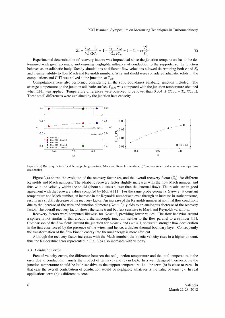
Figure 5: a)Overall temperature errors due to conduction in function of l/lc, b)Wire temperature distributions

Figure 5(a) represents the global contribution to the conduction error computed for the reference probe geom-etry (Geom1) for different materials. The figure compares for a given wire material and geometry, thus a givenl/lc, the variability of the temperature error due to the conditions at the shield/support. Fig. 5(b) displays thetemperature distribution along the wire in the same conditions for three of the materials and two of the boundaryconditions, adiabatic support and CHT within wire and support. The junction temperature (y = 0) is the same forthe ideal wire (l/lc = 37) independently of the conduction at the shield, with an overall conduction error about 0.04%. The temperature at each position along the wire is less affected by the longitudinal conduction, hence by theshield temperature, and more by the convective heat flux. Thus the temperature distribution is able to reflect thenon homogeneity of the gas temperature around the wire. The junction is only influenced by the wire temperatureadjacent to it, and the effect of the shield temperature penetrates until the last 20% of the wire. In the case ofconstantan wire the temperature along the wire is affected by conduction to the shield to a higher extent. However,the temperature at the junction converges to almost the same value for the different boundary conditions. Overallconduction errors vary between 0.18 and 0.19 %. In the copper wire case, with a l/lc about 2, conduction with thesupport influences the junction temperature in a higher degree. Errors vary between 0.23 and 0.45% depending onthe support conditions.

The reference adiabatic temperature considered for the analysis of the conduction errors is that of the junction.However, due to the strong flow deceleration taking place around the wire in the vicinity of the junction, there isa less efficient flow deceleration in this region. Thus, the temperature recovered is lower when compared to thejunction. This effect can be observed in Fig. 5(b) for the ideal wire distribution in which the temperatures at 10to 20 % from the junction are slightly lower than at the junction. It explains also the slight difference between thejunction temperatures for constantan and ideal material wires. The higher conductivity of constantan forces thejunction to stabilize at the lower temperature of the wire in the vicinity, while for the ideal material the temperatureat the junction rises to almost the adiabatic temperature.

6. Transient Temperature Effects

The diffusion of the heat fluxes within the probe introduce a temperature lag on the junction temperaturewith respect to the gas temperature. The properties and geometry of the thermocouple wires affect the junctiontemperature evolution.

The numerical methodology applied in this study allowed analyzing the temperature evolution on the completeprobe in response to a temperature step. All the results correspond to the nominal flow conditions, with an initialprobe temperature equal to Ti=300 K.

The temporal evolution of the temperature along the constantan wire for Geom1 is displayed in Fig.6. At eachposition along the wires, the rate of temperature change is different. The response time of the shield is much



0 . 0 0 . 5 1 . 0

2 9 9 . 5

3 0 0 . 0

y = 0 . 4 4

2 9 8 . 8 2 9 9 . 42 9 9 . 22 9 9 . 0T , K

t = 0 . 0 1 s t = 0 . 0 1 8 s t = 0 . 2 3 8 s t = 0 . 4 1 8 s t = 0 . 7 1 8 s S t e a d y C H T

T, K

y , m m

t

2 9 9 . 6

y = 0 y = 0 . 9 1

Figure 6: a)2D temperature contour, steady conditions. b) Evolution of constantan wire temperature distribution. CHT result

higher than that of the junction or wire due to its larger thermal inertia and lower thermal diffusivity a. Thus thepart of the wire closer to the junction y = 0 reached the final temperature faster than the part of the wire close tothe shield/support due to its influence by conduction. Figure 7 shows the time temperature history at three wirepositions and a point within the shield, for constantan and copper materials. The temperature traces are made nondimensional with their steady value in order to compare the response times, not taking into account the differenceson the final temperature achieved.

All the temperature distributions, except that of the shield, showed a fast initial temperature change, followedby a slower evolution. The fast initial temperature rise is dictated by the inertia of the junction or wire elements.The slow down is accentuated by the influence of the support at a certain position. In the constantan case thejunction overpassed the conventional threshold of the 63.2 % of the response in 6.5 ms, and achieved the 90%of the final temperature in 18 ms. The temperature at y = 0.44mm showed a faster initial rise due to the lowerthermal inertia of a wire element when compared with the junction, of bigger volume. However the convergenceto the final temperature takes longer than in the junction due to the influence of the evolution of the shield at thispoint. The same behavior was observed at y = 0.91, but influenced in a higher degree by the shield temperatureevolution.

The comparison of the temperature evolutions in the copper wire case, is analogous. When compared withthe constantan results, the initial response of the copper is slightly slower, and the temperature evolutions at thedifferent points closer in terms of the temperature rate evolution. It is explained by the higher conductivity ofthe copper, that implies higher diffusivity along the wire, and thus smoother temperature gradients between thedifferent positions. Whereas in the constantan case, the effect of the support is little felt close to the junction butgreatly affecting the opposite wire extreme.

In the ideal case of no existence of conductive heat between junction and wire, or if equal wire and junctiondiameters and no conduction flux with the support, the response of the thermocouple would be that of a firstorder system, Eq. 5. The characteristic would be the time required to complete 63.2 % of its response to a



0 . 0 0 0 . 0 4 0 . 0 80 . 0

0 . 5

1 . 0

(T-T g1

)/(Tf-T g1

)

t , s

J u n c t i o n y = 0 . 4 4 y = 0 . 9 1 y = 1 . 2 4

C o n s t a n t a n C o p p e r

Figure 7: Temperature evolution at four control points on constantan and copper wires

0 . 0 0 0 . 0 4 0 . 0 8

0 . 8

0 . 9

1 . 0

R e a l 1 s t o r d e r W I R E A D A D A D , y = 0 . 4 4 C H T

(T-T g1

)/(Tf-T g1

)

t , s

Figure 8: Comparison junction temporal evolutions with the correspondent first order.

gas temperature step. None of the wire temperature evolutions represented in Fig.7 corresponds to a first orderresponse due to the influence of the support.

Non dimensional junction temperature evolutions are represented in Fig. 8 for the ideal case of adiabaticwire, and constantan wire with two different support conditions: CHT and adiabatic. For each evolution the timeto reach 63.2% of the final temperature was used to evaluate the correspondent first order response. When thewires are considered adiabatic, the junction evolution collapses to the first order response. The presence of thewires modifies the temperature response whatever the condition at the support. When no flux occurs betweenshield and wires the junction reach the final temperature without the delay caused by the support but it does notcorrespond to a first order. This result is in agreement with the works of Yule [12] and Petit [6]. The influence ofthe wires causes an acceleration of the junction response if compared with the adiabatic wire result. It is instigatedby conductive effects from the faster response of a wire element. The evolution at y = 0.44 is included in thegraph for comparison. A simple decomposition in two first order systems expressing the response of the wireand support as done in cold wires [13] does not accurately reproduce the junction response in the presence ofconductive effects.

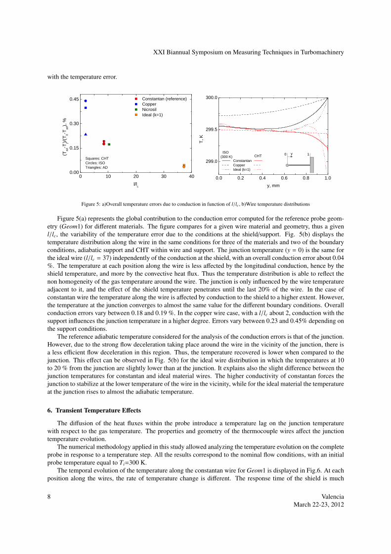
Figure 9 displays the non dimensional junction temperature evolutions for different wire materials and the twowire diameters (Geom1 and Geom2). All cases correspond to complete CHT simulations with the consequentpossible influence of the slower response of the support. For the cases in which the conductive effects on thejunction are not too noticeable (l/lc ≥ 5), the higher the wire conductivity the faster the response of a wire elementand therefore the faster the response of the junction. Increasing the wire and junction diameters introduces a delayin the response due to the increase of the thermal inertia, and a decrease of the parameter l/lc, hence an increase



0 . 0 0 0 . 0 4 0 . 0 8

0 . 8

0 . 9

1 . 0

(T-T g1

)/(Tf-T g1

)

t , s

C o n s t a n t a n N i c r o s i l C o p p e r I d e a l ( k = 1 )

G e o m 1 G e o m 2

Figure 9: Junction temporal evolution. CHT simulations

1 0 0 1 0 10 . 4

0 . 6

0 . 8

1 . 0

H

f , H z

W I R E A D C H T , i d e a l ( k = 1 ) C H T , N i c r o s i l C H T , C o n s t a n t a n A D , C o n s t a n t a n C H T , C o n s t a n t a n G e o m 2

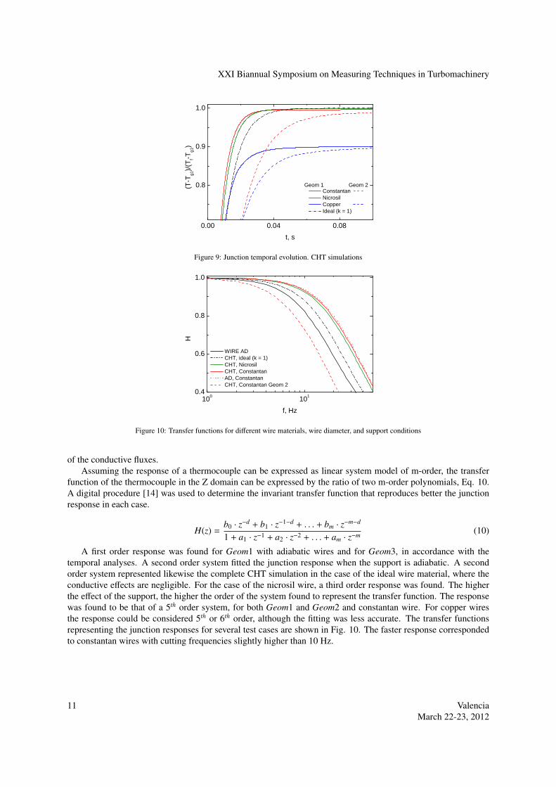
Figure 10: Transfer functions for different wire materials, wire diameter, and support conditions

of the conductive fluxes.Assuming the response of a thermocouple can be expressed as linear system model of m-order, the transfer

function of the thermocouple in the Z domain can be expressed by the ratio of two m-order polynomials, Eq. 10.A digital procedure [14] was used to determine the invariant transfer function that reproduces better the junctionresponse in each case.

H(z) =b0 · z−d + b1 · z−1−d + . . . + bm · z−m−d

1 + a1 · z−1 + a2 · z−2 + . . . + am · z−m (10)

A first order response was found for Geom1 with adiabatic wires and for Geom3, in accordance with thetemporal analyses. A second order system fitted the junction response when the support is adiabatic. A secondorder system represented likewise the complete CHT simulation in the case of the ideal wire material, where theconductive effects are negligible. For the case of the nicrosil wire, a third order response was found. The higherthe effect of the support, the higher the order of the system found to represent the transfer function. The responsewas found to be that of a 5th order system, for both Geom1 and Geom2 and constantan wire. For copper wiresthe response could be considered 5th or 6th order, although the fitting was less accurate. The transfer functionsrepresenting the junction responses for several test cases are shown in Fig. 10. The faster response correspondedto constantan wires with cutting frequencies slightly higher than 10 Hz.



7. Conclusions

A new methodology was proposed to numerically resolve the evolution of the heat transfer balances withina thermocouple probe. This procedure was applied to a shielded thin wire thermocouple, providing valuableinformation of the effect of the design parameters on the different error sources. This method overcame theexperimental difficulties providing detailed information of the performances of a given probe in the range of flowconditions of interest.

Results from conjugate heat transfer simulations were analyzed at different values of the main non dimensionalparameters driving the heat fluxes within the thermocouple probe. This approach allowed dissecting the commonlydescribed experimental ”recovery factor” into two steady error sources: flow velocity effects and conductive-convective errors. Radiation effects were shown to be negligible for the flow environment of interest.

Recovery factors for the shielded probe were computed at different Mach and Reynolds numbers. The tem-perature error increase due to velocity effects was evaluated, confirming the benefit of shield designs against barethermocouples at high velocities.

Temperature errors due to conduction were analyzed for different test cases. The influence of conductive errorson the junction temperature is mainly dictated by the parameter l/lc, which collects the effects of the wire conduc-tivity, length and diameter and flow convective heat transfer, and by the support characteristics. The decrease ofthe temperature error with increasing values of l/lc is reported. When values of the parameter l/lc higher than 5cannot be achieved, the junction temperature error is dominated by the wires support.

Time resolved CHT simulations allowed analyzing the temporal temperature evolution within the probe. Theeffect of the design parameters on temperature change rate was analyzed. The transfer function of the junctiontemperature response was obtained for the different tests simulated. The order of the lineal differential equationmodeling the response was shown to increase with the influence of the conductive effects from the support on thejunction. The response could be that of a second or third order differential linear system for l/lc values higher than10.

The presented methodology coupled with optimizers would provide a tool to design the best probe for a specificapplication.

Acknowledgments

This work was sponsored by TechSpace Aero in the frame of INTELLIGENT COOLING SYSTEM project.The financial support of the Region Wallone and the pole of competitiveness Skywin is acknowledged. The authorsare grateful to V. Van der Haegen for his valuable contribution on the numerical work.

References

[1] L. V. ne, G. Paniagua, M. Kaya, D. Bajusz, S. Hiernaux, Development of a Transonic Wind Tunnel to investigate Engine Bypass FlowHeat Exchangers, Proc. IMechE, Part G: J. Aerospace Engineering 225, 8 (2011) 902–914.

[2] G. E. Glawe, R. Holanda, L. N. Krause, Recovery and Radiation Corrections and Time Constants of Several Sizes of Shielded andUnshielded Thermocouple Probes for Measuring Gas Temperature, Tech. rep., Lewis Research Center, Cleveland, Ohio (1978).

[3] J. Rom, Y. Kronzon, Small shielded thermocouple total temperature probes, Tech. rep., Institute of Technology, Israel (1967).[4] T. M. Stickney, Recovery and time-response characteristics of six thermocouple probes in subsonic and supersonic flow, NACA TN

3455, Tech. rep., Lewis Flight Propulsion Laboratoty, Cleveland Ohio (1955).[5] H. I. H. Saravanamuttoo, Recommended practices for measurement of gas path pressures and temperatures for performance assessment

of aircraft turbine engines and components, Advisory Report 245, AGARD Advisory Report No. 245 (1990).[6] C. Petit, P. Gajan, J. C. Lecordier, P. Paranthoen, Frequency response of fine wire thermocouple, J. Phys. E: Sci. Instrum 15 (1982)

760–764.[7] M. D. Scadron, I. Warshawsky, Experimental determination of time constants and Nusselt numbers for bare wire thermocouples in high

velocity air streams and analytic approximation of conduction and radiation errors. NACA TN 2599, Technical Note 2599, Lewis FlightPropulsion LAboratory, Cleveland, Ohio (1952).

[8] C. H. H, A. Kalitinsky, Temperature measurements in high velocity air streams, Trans. ASME 67 (1945) A–25.[9] F. S. Simmons, Recovery Corrections for Butt Welded stright wire thermocouples in high velocity, high temperature gas streams, Tech.

rep., NACA RM-E54G22a (1954).[10] G. Glawe, F. S. Simmons, T. M. Stickney, Radiation and recovery corrections and time constants of several chromel-alumel thermocouple

probes in high temperature high velocity gas streams, Tech. rep., NACA TN-3766 (1956).[11] R. J. Moffat, Gas temperature measurement.



[12] A. J. Yule, D. S. Taylor, N. A. Chigier, Thermocouple Signal Processing and On-Line Digital Compensation, Journal of Energy 2, No 4(1978) 223–231.

[13] R. Dnos, C. Sieverding, Assessment of the cold wire resistance thermometer for high speed turbomachinery applications, Journal ofTurbomachinery 119, N0 1 (1997) 140–148.

[14] G. Paniagua, R. Dnos, Digital compensation of pressure sensors in the time domain, Experiments in Fluids 32, No 4 (2002) 417–424.


aerothermal analysis and characterization of shielded fine

Documents