turbine aerothermal optimization using evolution strategies
TRANSCRIPT

Turbine Aerothermal Optimization Using Evolution Strategies
by
Drew A. Curriston
A thesis submitted to the Graduate Faculty ofAuburn University
in partial fulfillment of therequirements for the Degree of
Master of Science
Auburn, AlabamaMay 4th, 2014
Keywords: Turbine, Optimization, Aerothermal, Bezier
Copyright 2014 by Drew A. Curriston
Approved by
Roy Hartfield, Chair, Walt and Virginia Woltosz Professor of Aerospace EngineeringBrain Thurow, Associate Professor of Aerospace Engineering
Andrew Shelton, Assistant Professor of Aerospace Engineering

Abstract
The use of adaptive optimizers in turbine blade geometry design is discussed. Many
different adaptive optimizers have been applied to turbine blade design in the past, but
often the optimizer does not fit the problem and unnecessary constraints are implemented.
This work analyzes the popular choices for turbine blade optimization, select the most fit-
ting optimizer that will lead to the lowest number of constraints, and apply it to an airfoil
optimization problem for validation. After validation, the optimizer is used in a turbine
blade optimization problem considering aerodynamics and convective heat transfer in the
objective function. The algorithm uses a 2D Navier-Stokes blade-to-blade analysis to evalu-
ate the effectiveness of the solution encoding and optimizer performance. By using a highly
effective optimizer for the specified problem, the computation time is drastically reduced
while producing comparable or better results, and these benefits will also allow the use of a
higher fidelity analysis without excessive computational costs.
ii

Acknowledgments
I would like to thank my wife Meg, and my children Cally, Joshua, Jacob, and Asher for
their continued support in completing this paper. I would also like to thank Dr. Hartfield
for the time and effort have gave while advising me on this research, and Dr. Shelton for
lending his expertise in helping me understand and implement CFD.
iii
Table of Contents
Abstract . . . . . . . . . . . . . . . . . . . . . . . . . . . . . . . . . . . . . . . . . . . ii
Acknowledgments . . . . . . . . . . . . . . . . . . . . . . . . . . . . . . . . . . . . . . iii
List of Figures . . . . . . . . . . . . . . . . . . . . . . . . . . . . . . . . . . . . . . . vi
List of Tables . . . . . . . . . . . . . . . . . . . . . . . . . . . . . . . . . . . . . . . . x
1 Introduction . . . . . . . . . . . . . . . . . . . . . . . . . . . . . . . . . . . . . . 1
1.1 Objectives . . . . . . . . . . . . . . . . . . . . . . . . . . . . . . . . . . . . . 1
1.1.1 Objective 1: Produce and Validate Optimizer . . . . . . . . . . . . . 2
1.1.2 Objective 2: Turbine Aerodynamic Optimization . . . . . . . . . . . 2
1.1.3 Objective 3: Turbine Aerothermal Optimization . . . . . . . . . . . . 2
1.2 Literature Review . . . . . . . . . . . . . . . . . . . . . . . . . . . . . . . . . 3
1.3 Problem Background . . . . . . . . . . . . . . . . . . . . . . . . . . . . . . . 5
2 Evolution Strategies . . . . . . . . . . . . . . . . . . . . . . . . . . . . . . . . . 8
2.1 Algorithm Selection . . . . . . . . . . . . . . . . . . . . . . . . . . . . . . . . 8
2.2 Solution Encoding and Move Operator . . . . . . . . . . . . . . . . . . . . . 12
2.3 Optimizer Validation . . . . . . . . . . . . . . . . . . . . . . . . . . . . . . . 18
2.3.1 Validation Case 1 . . . . . . . . . . . . . . . . . . . . . . . . . . . . . 18
2.3.2 Validation Case 2 . . . . . . . . . . . . . . . . . . . . . . . . . . . . . 24
2.3.3 Conclusions From Optimizer Validation . . . . . . . . . . . . . . . . . 26
3 Turbine Aerodynamic Optimization . . . . . . . . . . . . . . . . . . . . . . . . . 28
3.1 Turbine Fundamentals Review . . . . . . . . . . . . . . . . . . . . . . . . . . 28
3.2 Preliminary Inviscid Analysis . . . . . . . . . . . . . . . . . . . . . . . . . . 30
3.2.1 Model and Assumptions . . . . . . . . . . . . . . . . . . . . . . . . . 30
3.2.2 Grid Generation and CFD Code . . . . . . . . . . . . . . . . . . . . . 31
iv
3.2.3 Objective Function . . . . . . . . . . . . . . . . . . . . . . . . . . . . 32
3.2.4 Results and Optimizer Performance . . . . . . . . . . . . . . . . . . . 33
3.3 Viscous Turbine Analysis . . . . . . . . . . . . . . . . . . . . . . . . . . . . . 37
3.3.1 Model and Assumptions . . . . . . . . . . . . . . . . . . . . . . . . . 38
3.3.2 Optimizer Updates and Objective Function . . . . . . . . . . . . . . . 39
3.3.3 Structural Considerations . . . . . . . . . . . . . . . . . . . . . . . . 42
3.3.4 Results and Optimizer Performance . . . . . . . . . . . . . . . . . . . 43
4 Turbine Aerothermal Optimization . . . . . . . . . . . . . . . . . . . . . . . . . 48
4.1 Heat Transfer Model . . . . . . . . . . . . . . . . . . . . . . . . . . . . . . . 48
4.2 Adaptations to Optimizer . . . . . . . . . . . . . . . . . . . . . . . . . . . . 49
4.2.1 Objective Function . . . . . . . . . . . . . . . . . . . . . . . . . . . . 49
4.3 Preliminary Aerothermal Optimization Results . . . . . . . . . . . . . . . . . 51
4.3.1 Issues With Preliminary Results . . . . . . . . . . . . . . . . . . . . . 53
4.3.2 Updates to Objective Function . . . . . . . . . . . . . . . . . . . . . 54
4.3.3 Stage Aerothermal Results . . . . . . . . . . . . . . . . . . . . . . . . 55
5 Conclusions and Future Applications . . . . . . . . . . . . . . . . . . . . . . . . 62
Bibliography . . . . . . . . . . . . . . . . . . . . . . . . . . . . . . . . . . . . . . . . 64
Appendices . . . . . . . . . . . . . . . . . . . . . . . . . . . . . . . . . . . . . . . . . 67
A Pseudo Code for ESTurb . . . . . . . . . . . . . . . . . . . . . . . . . . . . . . . 68
B Example GRAPE and RVCQ3D input files . . . . . . . . . . . . . . . . . . . . . 69
C Additional Plots for Optimization Runs . . . . . . . . . . . . . . . . . . . . . . 71
D Off-Design Effects on Aerothermal Blade . . . . . . . . . . . . . . . . . . . . . . 74
E Brief Grid Refinement Study . . . . . . . . . . . . . . . . . . . . . . . . . . . . . 76
v

List of Figures
1.1 Example Velocity Diagrams for a Stator[21] . . . . . . . . . . . . . . . . . . . . 6
1.2 Example Velocity Diagrams for a Rotor[21] . . . . . . . . . . . . . . . . . . . . 6
2.1 Search space comparison for minimization problem . . . . . . . . . . . . . . . . 12
2.2 PARSEC encoding . . . . . . . . . . . . . . . . . . . . . . . . . . . . . . . . . . 14
2.3 Example of using Bezier curves to encode blade[23] . . . . . . . . . . . . . . . . 14
2.4 Spline connected polynomial encoding angles and radii[21] . . . . . . . . . . . . 14
2.5 Spline connected polynomial encoding defining points[21] . . . . . . . . . . . . . 14
2.6 Blade surface for example solution encoding . . . . . . . . . . . . . . . . . . . . 15
2.7 Move operator example for a single control point . . . . . . . . . . . . . . . . . 17
2.8 Second control point mutation option 1 . . . . . . . . . . . . . . . . . . . . . . . 18
2.9 Second control point mutation option 2 . . . . . . . . . . . . . . . . . . . . . . . 18
2.10 Flow chart for ESTurb algorithm . . . . . . . . . . . . . . . . . . . . . . . . . . 19
2.11 Test case one objective function results (sought to minimize) . . . . . . . . . . . 21
2.12 Test case one computation time comparison . . . . . . . . . . . . . . . . . . . . 21
2.13 XFoil output for converged airfoil . . . . . . . . . . . . . . . . . . . . . . . . . . 22
vi
2.14 History of objective function value over generations for initial eight runs . . . . 23
2.15 Example of variation in final population from Figure 2.13 . . . . . . . . . . . . . 23
2.16 Pareto front results . . . . . . . . . . . . . . . . . . . . . . . . . . . . . . . . . . 26
2.17 Pareto front progression with computation time . . . . . . . . . . . . . . . . . . 27
3.1 Elliptical H-grid . . . . . . . . . . . . . . . . . . . . . . . . . . . . . . . . . . . 31
3.2 Leading edge without vertical clustering . . . . . . . . . . . . . . . . . . . . . . 31
3.3 Leading edge with vertical clustering . . . . . . . . . . . . . . . . . . . . . . . . 31
3.4 Euler code validation results . . . . . . . . . . . . . . . . . . . . . . . . . . . . . 32
3.5 Objective function values over 50 generations . . . . . . . . . . . . . . . . . . . 35
3.6 Final blade geometry using spline-connected polynomial encoding . . . . . . . . 35
3.7 Final blade geometry using Bezier curve encoding . . . . . . . . . . . . . . . . . 36
3.8 Example 169x45 grid for VK-LS89 turbine blade . . . . . . . . . . . . . . . . . 40
3.9 Close-up of trailing edge for VK-LS89 turbine blade grid . . . . . . . . . . . . . 41
3.10 Blade geometry and pressure contour results for single stage . . . . . . . . . . . 45
3.11 Mach Number contours for stator . . . . . . . . . . . . . . . . . . . . . . . . . . 46
3.12 Absolute Mach Number contours for rotor . . . . . . . . . . . . . . . . . . . . . 47
4.1 Ideal engine power vs. pressure ratio . . . . . . . . . . . . . . . . . . . . . . . . 51
4.2 Relationship for normalized power ratio vs turbine inlet temperature . . . . . . 51
vii

4.3 Aerothermal run 1 pressure contours . . . . . . . . . . . . . . . . . . . . . . . . 52
4.4 Aerothermal run 2 pressure contours . . . . . . . . . . . . . . . . . . . . . . . . 52
4.5 Aerothermal run 3 pressure contours . . . . . . . . . . . . . . . . . . . . . . . . 52
4.6 Preliminary aerothermal results: Heat transfer coefficient . . . . . . . . . . . . . 52
4.7 Aerothermal run 1 Mach number distribution . . . . . . . . . . . . . . . . . . . 54
4.8 “Bump” in velocity distribution for turboprop blade[3] . . . . . . . . . . . . . . 54
4.9 Stage aerothermal Run 1 stator Mach number distribution . . . . . . . . . . . . 56
4.10 Stage aerothermal Run 1 rotor Mach number distribution . . . . . . . . . . . . 56
4.11 Comparison of final stator geometries . . . . . . . . . . . . . . . . . . . . . . . . 57
4.12 Comparison of final rotor geometries . . . . . . . . . . . . . . . . . . . . . . . . 57
4.13 Stage pressure contours for Run 1 . . . . . . . . . . . . . . . . . . . . . . . . . . 58
4.14 Types of leading edges and incidence angle effects[3] . . . . . . . . . . . . . . . 59
4.15 Heat transfer coefficient for optimized stator . . . . . . . . . . . . . . . . . . . . 60
4.16 Convergence history for both stator and rotor . . . . . . . . . . . . . . . . . . . 61
C.1 Pressure contours for Run 2 stage results . . . . . . . . . . . . . . . . . . . . . . 72
C.2 Isentropic Mach number distribution for Run 2 stator . . . . . . . . . . . . . . . 72
C.3 Isentropic Mach number distribution for Run 2 rotor . . . . . . . . . . . . . . . 72
C.4 Pressure contours for Run 3 stage results . . . . . . . . . . . . . . . . . . . . . . 73
viii

C.5 Isentropic Mach number distribution for Run 3 stator . . . . . . . . . . . . . . . 73
C.6 Isentropic Mach number distribution for Run 3 rotor . . . . . . . . . . . . . . . 73
D.1 Mach number surface distribution over a range of incidence angles . . . . . . . . 75
D.2 Close-up of Figure D.1 suction side . . . . . . . . . . . . . . . . . . . . . . . . . 75
E.1 RRMS plot for 169x45 grid . . . . . . . . . . . . . . . . . . . . . . . . . . . . . 77
E.2 Mach number distribution for multiple grid sizes . . . . . . . . . . . . . . . . . 78
E.3 Heat transfer coefficient distribution for multiple grid sizes . . . . . . . . . . . . 78
ix

List of Tables
2.1 Example solution encoding . . . . . . . . . . . . . . . . . . . . . . . . . . . . . 15
4.1 Preliminary Aerothermal Results Summary . . . . . . . . . . . . . . . . . . . . 51
4.2 Stage Aerothermal Results Summary . . . . . . . . . . . . . . . . . . . . . . . . 56
x
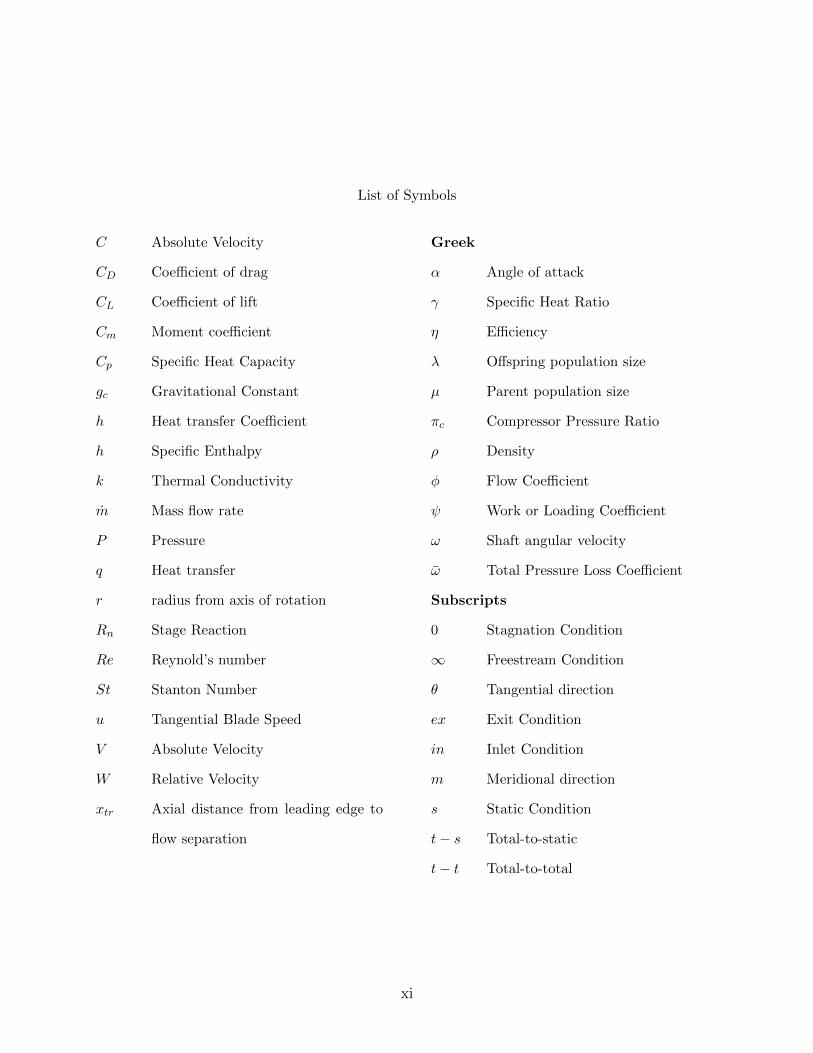
List of Symbols
C Absolute Velocity
CD Coefficient of drag
CL Coefficient of lift
Cm Moment coefficient
Cp Specific Heat Capacity
gc Gravitational Constant
h Heat transfer Coefficient
h Specific Enthalpy
k Thermal Conductivity
m Mass flow rate
P Pressure
q Heat transfer
r radius from axis of rotation
Rn Stage Reaction
Re Reynold’s number
St Stanton Number
u Tangential Blade Speed
V Absolute Velocity
W Relative Velocity
xtr Axial distance from leading edge to
flow separation
Greek
α Angle of attack
γ Specific Heat Ratio
η Efficiency
λ Offspring population size
µ Parent population size
πc Compressor Pressure Ratio
ρ Density
φ Flow Coefficient
ψ Work or Loading Coefficient
ω Shaft angular velocity
ω Total Pressure Loss Coefficient
Subscripts
0 Stagnation Condition
∞ Freestream Condition
θ Tangential direction
ex Exit Condition
in Inlet Condition
m Meridional direction
s Static Condition
t− s Total-to-static
t− t Total-to-total
xi
Chapter 1
Introduction
Gas turbine engines are used widely across the world for power generation, commercial
and military aircraft, and even ground vehicles. Their high power to weight ratio prove
especially fitting for aviation purposes, and the demand for efficient and powerful engines is
extremely high. Optimization of these systems in the preliminary design stage is generally
well understood and several books have been written on the subject, but the optimization
process for the detailed design of specific components is still an area of ongoing research. A
deterministic optimization approach is often not possible due to the high number of design
variables and complexity of the flow analysis, as well as the high possibility of the search
stopping in a local optimum. Global optimization techniques are often effective for problems
such as turbine design, but are inefficient in comparison, often requiring thousands of function
evaluations to produce a worthwhile result. Although this may prove possible with a simple
through-flow analysis code, using a full 3D Navier-Stokes analysis could require months or
years to complete, which is an unreasonable amount of computation time. Finding a more
efficient optimizer that finds a global optimum in only a few hundred function evaluations
or less would prove extremely useful in allowing a higher fidelity analysis and optimization
without excessive computational costs.
1.1 Objectives
The objectives of this paper include producing and validating an optimizer that is
both effective and efficient at evaluating turbine cascade problems, conduct an aerodynamic
optimization of a multi-stage turbine, and conduct an aerothermal optimization of the same
multi-stage turbine. These objectives are discussed in detail below.
1

1.1.1 Objective 1: Produce and Validate Optimizer
This objective includes evaluating a number of global optimizers, noting their strengths
and weaknesses, and selecting the appropriate optimizer for a turbine design problem that
capitalizes on it’s canonical strengths. This objective focuses on using a canonical, or close
to canonical, optimizer and limit the use of unreliable and problem specific optimizer en-
hancements. The optimizer has been written by the author and validated using a number
of test cases where the results are compared against published articles to evaluate optimizer
performance.
1.1.2 Objective 2: Turbine Aerodynamic Optimization
The optimizer has been applied to a turbine aerodynamic optimization problem. This
analysis includes a preliminary 2D inviscid analysis as well as a 2D Navier Stokes analysis. In
order to provide a comparison for results, the optimized blade geometry was evaluated against
the blade geometry of the T55-GA-714A engine currently used on the CH-47D Chinook
helicopter.
1.1.3 Objective 3: Turbine Aerothermal Optimization
The third objective improves on the aerodynamic optimization by investigating the
effects of blade geometry on the aerodynamic efficiency and overall convective heat transfer
to the blade. This optimization seeks to produce turbine blade geometries that allow a
higher turbine inlet temperatures due to reduced hot spots, while maintaining a high level
of aerodynamic performance. Higher turbine inlet temperatures may be directly correlated
to increased total power output and decreased specific fuel consumption[1]. This objective
includes an investigation into whether a blade geometry that allows higher turbine inlet
temperatures and slightly lower aerodynamic performance may prove to be a more optimal
blade.
2

1.2 Literature Review
The literature reviewed for this research included a variety of books on turbine design
and a number of published articles researching optimization, turbine design, and CFD spe-
cific topics. Although a large number of books were referenced in this paper, the books
most heavily referenced for detailed turbine blade design were Turbine Aerodynamics by
Ronald Aungier[2] and Principles of Turbomachinery in Air-Breathing Engines by Erian
Baskharone[3]. Both of these books provided a thorough walk-through of detailed blade
design that was well written and easy to understand. Baskharone’s text also provided case
studies that were helpful in understanding the fundamentals of blade design. Because both
of these references were written within the past 10 years, they represent a fairly up to date
review of current design techniques and processes, including detailed blade geometry design.
Wilson’s text[4] was also referenced heavily for preliminary and stage design. The methods
presented in these books were viewed by the author as the most current methods for blade
parameterization and design, and are therefore used as a basis for comparison.
CFD is a quickly growing field of study and is a very integral part of current turbo-
machinery research. Fluid Dynamics and Heat Transfer of Turbomachinery [5] by Lakshmi-
narayana along with the user’s manual for the CFD code were the main references used by
the author to ensure responsible CFD utilization. All CFD validation studies were conducted
in reference to Arts[6] due to the fact that it is commonly cited and used for CFD validation
in other publications. Articles by Horlock & Denton[7] as well as Denton & Dawes[8] provide
a background of CFD use in turbomachinery design compared to traditional methods over
the last 50 years. Because the focus of this thesis is on the performance of the optimizer
and a 2D blade-to-blade optimization, a well known and validated CFD code will be used
rather than conducting a literature study to find the most current CFD techniques. Several
articles have been written by Dr. Chima on the use and validation of the primary CFD code
used in this thesis, Rotor Viscous Code Quasi-3D (RVCQ3D), and all have been reviewed in
detail by the author.[9][10][11][12]
3

Optimization of turbomachinery using metaheuristics is a much more recent topic and
is not yet preferred over the traditional design methods. Research in this field is much more
sporadic and to the author’s knowledge no consolidated reviews of this topic exist. A number
of articles using stochastic algorithms to optimize turbine blades were reviewed by the author
and a summary of the more relevant articles is given in this literature review. The earliest
articles using metaheuristics to optimize blade shape appeared in the mid-1990’s. Turbine
Airfoil Design Optimization by Goel[13] was published in 1996 and used both circular arcs
and Bezier curves to represent the blade geometry. Several articles followed in 1998 and
1999 including two by Giannakoglou[14] [15], and articles by Pierret[16], Trigg[17], and
Dennis[18]. Each conducted an aerodynamic optimization using either a Genetic Algorithm
or Artificial Neural Network and used a very similar blade parameterization technique with
large restrictions on the movement of the control points. More recent work includes 3D
blade optimization using GAs as in articles by Chen[19] and Oksuz[20], which use Non-
Uniform Rational B-Splines (NURBS) to parameterize the blades but maintain circular
arc segments at the leading and trailing edges. In addition to those listed, several other
articles were reviewed and all had two common factors. The first is the use of constraints
to restrict the blade parameterization, either through limiting the movement of the control
points, using prescribed circular arc segments, or using a lower fidelity blade parameterization
method altogether. The second is conducting a purely aerodynamic optimization without
considering heat transfer and sometimes structural requirements as well. It was also apparent
that Genetic Algorithms were the optimizer of choice, with only one article using a different
optimizer.
The main reason metaheuristic optimizers are not preferred over traditional blade de-
sign methods is the high computational cost. However, analyzing several objective functions
at once, such as aerodynamic, thermal, and mechanical considerations, may make the com-
putational time more reasonable compared to doing each step manually. Less restrictions on
4

the search space may also find better solutions, especially when multiple objectives are con-
sidered. Therefore, more research is needed in this area, where there are very few published
articles available.
1.3 Problem Background
Turbine design is a very complex subject, but is also well documented by several books
that break down the steps of preliminary design into a manageable problem[4][1][2][3]. De-
tailed stage or blade design is a much more ambiguous topic with numerous methods available
in literature. These methods of detailed design usually rely on a large amount of practical
experience on the part of the engineer and knowledge of current best practices. The direct
blade design is usually preferred over the inverse design method, and one of a number of blade
curvature procedures is used along with manual iteration until a desirable blade is achieved.
This process provides ample opportunity for improvement upon using recent advanced in 2D
and 3D turbine modeling programs.
In order to understand the applicability of the detailed design process discussed in this
paper, it is important to first understand the preliminary design process. The preliminary
design process outlined here is a summary of the discussion in The Design of High-Efficiency
Turbomachinery and Gas Turbines by Wilson and Korakianitis[4]. The design process starts
with a number of given turbine specifications, which are listed below.
1. the fluid to be used
2. the fluid stagnation temperature and pressure at inlet
3. the fluid stagnation or static pressure at outlet
4. fluid mass flow or turbine power output required
5. shaft speed
5

Figure 1.1: Example Velocity Diagramsfor a Stator[21]
Figure 1.2: Example Velocity Diagramsfor a Rotor[21]
An initial investigation is usually conducted to determine if a single stage configuration
will suffice for the design. If the stage loading is too high, a multi-stage turbine must be
used and a stage work split is specified. With this given information and an assumption
of the inlet and exit flow angles, the velocity triangles for the turbine may be specified.
Velocity triangles depicting the inflow and outflow velocities and angles for each blade row
are a fundamental concept in turbine design, and an example is shown in Figures 1.1 and
1.2 . The velocity triangles are determined from the design work output requirements for
the engine and then the blade profiles are designed to match the velocity triangles, not the
other way around. The concept of velocity triangles is based on the Euler turbine equation.
A modified version of this equation is shown as Eqn. 1.1, which states that the enthalpy
change across a blade row is a function of the shaft speed, mean blade radius, and the change
in tangential velocity.
H2 −H1 = ω(r2Cθ2 − r1Cθ1) (1.1)
In order do define the velocity triangles three parameters are required: the work (or
loading) coefficient ψ, the flow coefficient φ, and the stage reaction Rn. These parameters
are discussed in detail in Wilson[4] and calculated using Eqns. 1.2-1.4. Velocity triangles are
often calculated from initial guesses for flow angles and then the stage reaction is checked. If
6

the stage reaction is unsatisfactory, the flow angles are adjusted and iterations are completed
until the desired stage reaction is obtained.
ψ =−gc∆ex
inh0u2
= −[
∆exin(uCθ)
u2
](1.2)
φ =Cmu
(1.3)
Rn =∆hs,rotor∆h0,stage
(1.4)
After velocity triangles for the mean line and other radial locations are obtained, the
number of blades per row, blade shape, and blade size may be determined. This detailed
design of the blade rows will be the focus of this paper. In order to focus on the detailed
blade design, it will be assumed that the prior preliminary design steps have already been
completed. The data from the T55-GA-714 engine will be used as a starting point for this
analysis, including the velocity triangles, annulus geometry, shaft speed, and thermodynamic
properties at each stage location. It is important to note that the information used in this
analysis from the T55 engine design report is proprietary to Honeywell International Inc.
and will not be disclosed in this report. All comparisons between optimized results and the
original T55 geometry will be presented as ratios or percentages to protect this information.
7

Chapter 2
Evolution Strategies
2.1 Algorithm Selection
A variety of meta-heuristic optimizers are available to apply to this problem, and choos-
ing the appropriate one will have a great influence on the final results. Although many
different types of optimizers have been applied to turbine optimization problems in the past,
not all of them fit the problem at hand. Because this is a continuous problem, optimizers
that are strong at solving combinatorial problems but are weak in a continuous solution space
will not be considered. These include Tabu Search, Ant Colony optimizers, and others. To
narrow the choice of optimizers further it is desirable to obtain a variety of near-optimal
results at the end of an optimization process, and therefore non-population based optimiz-
ers such as Simulated Annealing would not be as advantageous. Three primary population
based optimizers that often perform well for aerodynamic problems are Genetic Algorithms
(GA), Evolution Strategies (ES), and Particle Swarm Optimizers (PSO). A short descrip-
tion of each is given below, and a much more detailed description may be found in the book
Metaheuristics for Hard Optimization[22].
Genetic Algorithms are based on the premise of natural selection and small evolutionary
changes. In the algorithm, members of an initial population of solutions are combined in
some sort of fashion to produce “offspring” that bear some of the characteristics of the
parents. These solutions are canonically represented as a bit string, but may also be a series
of real numbers that define a solution for the problem. Several offspring are produced and
then evaluated based on some function that determines fitness, an this objective function
may either be maximized or minimized for the particular problem. At this point the group of
parents and offspring are ordered by fitness and the most fit solutions become the parents for
8
a new generation while the remainder are discarded. This process is repeated until some pre-
determined stopping criteria is met, such as a maximum number of generations. A mutation
is usually included as well, which selects and perturbs a solution at random to increase
diversity in the population. This mutation rate is often very low, such as a few percent of
the offspring or less. After a large number of generations, the solutions will continue to get
better until they converge on a near-optimal solution. GAs have proven to be very successful
in finding the global optimum for a variety of problems. They do not easily get stuck in local
minimums, provide multiple solutions, and are easy to implement. However, GAs can be
very inefficient for certain problems, especially if the solution space is not well defined or the
initial solutions are difficult to randomly place across the breadth of the solution space. GAs
generally require a larger population size as well to ensure enough variation in the offspring
to make an effective search.
Particle Swarm Optimizers are inspired by birds flocking together or fish swimming
in a school. In this algorithm a population of solutions, or “particles”, move through the
solution space using a velocity that is updated after each move. Each member’s velocity
is updated based on it’s own inertia, the location of the best solution seen by the particle,
and the location of the best solution seen by anyone in communication with the particle.
The algorithm uses this collective knowledge of the swarm to locate the global optimum in
the solution space. There are a number of variations and enhancements to the PSO algo-
rithm, such as limiting the communication to neighborhoods in the particles and limiting the
maximum velocity. In general, the PSO algorithm is very easy to implement and converges
fairly fast. Disadvantages of this algorithm include being stuck in local optimum easier than
other meta-heuristics and sensitivity to input parameters. The ability of a PSO to find the
global optimum is highly dependent on the location of the initial population in relation to
the optimum and the starting inertia of each particle.
Evolution Strategies algorithms are very similar to GAs, and in fact were developed
in Europe around the same time as GAs in the 1970s. As in GAs, ES algorithms use a
9
population of solutions to produce offspring, sort the offspring based on a fitness value, and
select a certain number of offspring to proceed as the parents of the following generation.
The difference between GAs and ES algorithms is the move operator, which is the method of
producing offspring. In an ES algorithm 100% of the offspring are mutated from the parent
solutions. This is accomplished through a random perturbation using a normal distribution
and a standard deviation value σ. After the designated number of offspring have been
mutated from the parent solutions, the solutions are sorted and the most fit will proceed to
the next generation. This move operator will be discussed in more detail in the following
sections. ES algorithms are easy to setup, can easily handle problem constraints and find
global optimum, and have the ability to self-adjust parameters during the optimization
process to adapt to the search space. They also perform well with micro-populations of
only a few members because the σ value controls the diversity of the search instead of the
diversity in the parent population. Disadvantages of ES algorithms include the possibility
of getting stuck in a local optimum if the parent population is far from the global optimum
and the σ values are not sufficient enough to move the solutions the required distance.
Although any of these three algorithms would be capable of finding a optimal or near
optimal solution, performance may vary greatly between the three based on their canonical
form and how they are chosen to be implemented. In an aerodynamic optimization problem,
an algorithm that searches fast and requires relatively few function evaluations is desired
because each function evaluation may be extremely costly, especially if a Navier-Stokes
solver is used for the evaluation. The limits of the search space are also very difficult to
determine in aerodynamic problems, if they can be determined at all. Sometimes random
initial solutions are used, but more often a known good solution is used as the starting point.
Therefore, an algorithm that can search outward as efficiently as it can search inward would
be desirable. A simple, robust algorithm is also very beneficial due to the long optimization
times. If the optimization process only required a few seconds or minutes to complete it
10

would be simple to restart if a problem occurred, but for an optimization process that takes
several hours or days a robust algorithm becomes extremely important.
Considering the characteristics desired in an algorithm for turbine optimization, Evo-
lution Strategies is the most appropriate meta-heuristic for this problem. The larger pop-
ulation sizes required to make GAs and PSOs effective would greatly increase computation
time while using a micro-population with an ES algorithm would drastically reduce the num-
ber of required function evaluations. Airfoil and blade geometry poses an inherent problem
with the move operators in genetic algorithms and PSOs because these algorithms work best
when the initial solutions are randomly placed across the breadth of the search space. This
typically does not happen in airfoil optimization because the limits of the search space are
often unknown, and the author often chooses a set of known airfoil geometries as the starting
points. Move operators in GAs and PSOs are more inclined to move inward towards the
local and global optima and do so very quickly and efficiently, while outward movement past
the initial starting points is slower and more difficult. In order to move outside the area of
the search space bounded by the parent solutions, GAs must wait for a random mutation
to occur that moves the solution in the right direction. Canonically the mutation rate in a
GA is very low, usually less than 2%, and the mutation is randomly generated such as a bit
flip or a random number generation. This is often overcome by raising the mutation rate to
much higher levels, but this only results in less effective version of an ES algorithm and an
inefficient search. PSOs also have difficulty moving outside the bounds of the initial parent
population if the inertia from the initial velocities cannot carry the particles far enough to
get close to the global optimum. An example of a minimization problem is shown in Figure
2.1 with white stars depicting the initial solutions. The example on the left is well suited
for a genetic algorithm or a PSO because the limits of the search space are well defined and
random initial solutions can be placed across the breadth of the search space. The example
on the right is more typical for an airfoil optimization problem, where the initial solutions
11
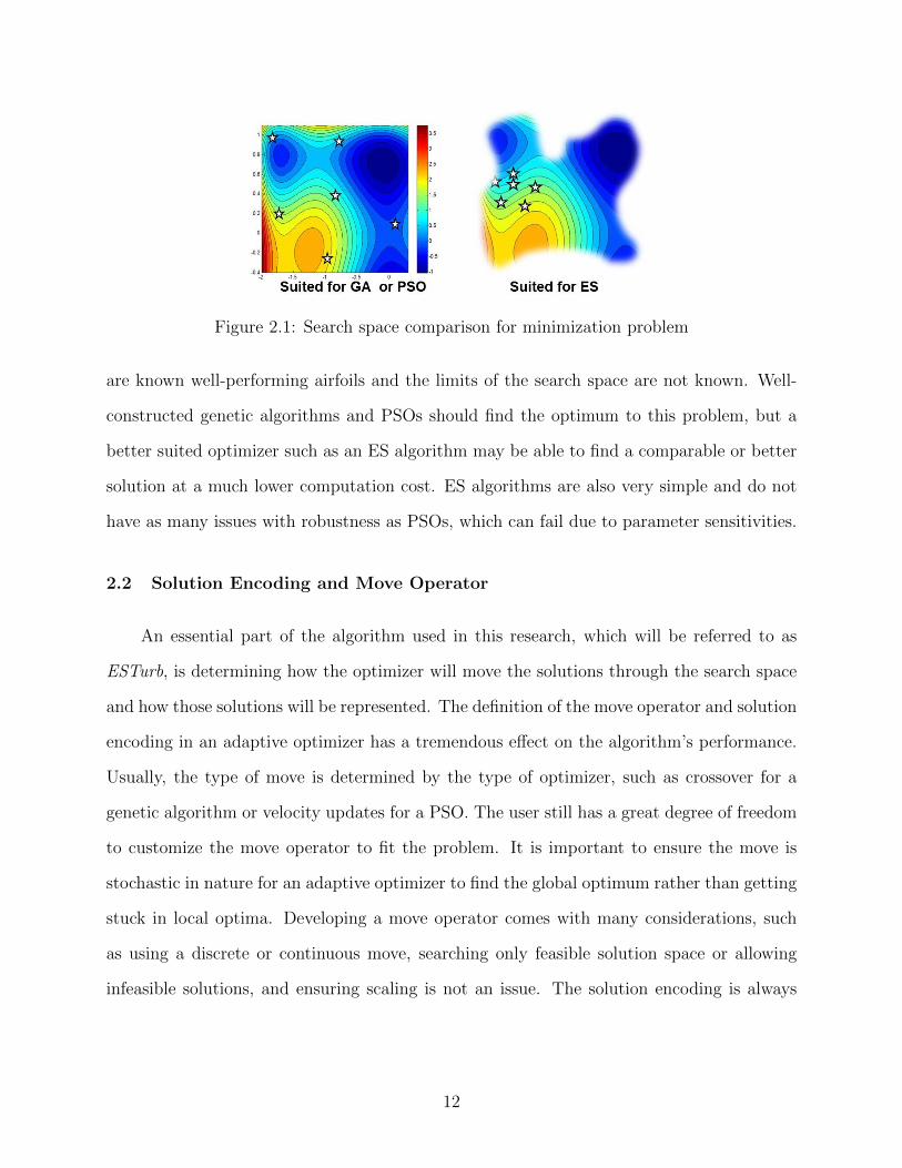
Figure 2.1: Search space comparison for minimization problem
are known well-performing airfoils and the limits of the search space are not known. Well-
constructed genetic algorithms and PSOs should find the optimum to this problem, but a
better suited optimizer such as an ES algorithm may be able to find a comparable or better
solution at a much lower computation cost. ES algorithms are also very simple and do not
have as many issues with robustness as PSOs, which can fail due to parameter sensitivities.
2.2 Solution Encoding and Move Operator
An essential part of the algorithm used in this research, which will be referred to as
ESTurb, is determining how the optimizer will move the solutions through the search space
and how those solutions will be represented. The definition of the move operator and solution
encoding in an adaptive optimizer has a tremendous effect on the algorithm’s performance.
Usually, the type of move is determined by the type of optimizer, such as crossover for a
genetic algorithm or velocity updates for a PSO. The user still has a great degree of freedom
to customize the move operator to fit the problem. It is important to ensure the move is
stochastic in nature for an adaptive optimizer to find the global optimum rather than getting
stuck in local optima. Developing a move operator comes with many considerations, such
as using a discrete or continuous move, searching only feasible solution space or allowing
infeasible solutions, and ensuring scaling is not an issue. The solution encoding is always
12

problem dependent, but must work well with the move operator to produce an effective
algorithm.
When selecting a solution encoding there are several factors to be considered. The
encoding must fully represent the solution, which is the upper and lower surface curves of
the turbine blade, in as few variables as possible. Choosing two few variables would not
fully represent the solution and adding too many variables, such as a series of coordinate
pairs to describe the blade surface, would add so many dimensions to the problem that the
search space would be unreasonably large. The solution encoding must also limit unnec-
essary restrictions to the search space which could not allow an optimum solution to be
represented. Obviously, if the optimum solution cannot be encoded, then it cannot be found
by the algorithm. A good solution encoding for an aerodynamic problem should be able
to represent almost any feasible airfoil using a small number of variables, and maintain a
smooth continuous curve for the blade surfaces. There are a number of options available,
such as the 11 variable PARSEC encoding shown in Figure 2.2, spline connected polyno-
mial segments shown in Figures 2.4 and 2.5, or a series of polynomial curves such as Bezier
Curves as shown in Figure 2.3. Most parameterization methods have inherent restrictions
on representing certain geometries, such as the problem PARSEC encoding has with fully
describing the trailing edge of an airfoil. Bezier Curves are used in ESTurb due to it’s ability
to represent almost any curve, ease of use, and small number of variables. Bezier Curves
are a form of parametric curve where the polynomial coefficients are controlled through a
number of control points. When Bezier Curves are used with other optimizers the control
points are almost always limited to certain regions in order to define the limits of the search
space and allow a more effective search for a GA or PSO. An example of this is the boxes
depicting the limits for each control point shown in Figure 2.3. However, these restrictions
prevent the algorithm from representing a large portion of the search space, which may
include the optimum solution. By using an ES algorithm in ESTurb these restrictions are
not necessary because the algorithm searches outward very effectively. This may allow the
13
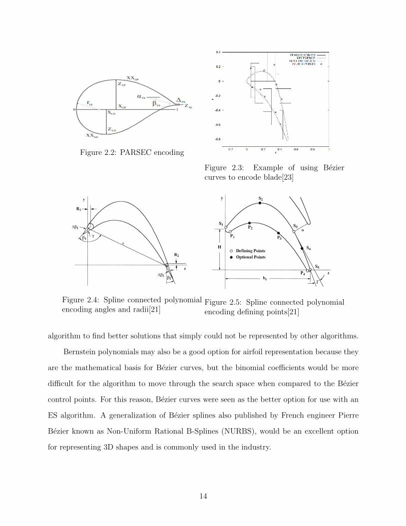
Figure 2.2: PARSEC encoding
Figure 2.3: Example of using Beziercurves to encode blade[23]
Figure 2.4: Spline connected polynomialencoding angles and radii[21]
Figure 2.5: Spline connected polynomialencoding defining points[21]
algorithm to find better solutions that simply could not be represented by other algorithms.
Bernstein polynomials may also be a good option for airfoil representation because they
are the mathematical basis for Bezier curves, but the binomial coefficients would be more
difficult for the algorithm to move through the search space when compared to the Bezier
control points. For this reason, Bezier curves were seen as the better option for use with an
ES algorithm. A generalization of Bezier splines also published by French engineer Pierre
Bezier known as Non-Uniform Rational B-Splines (NURBS), would be an excellent option
for representing 3D shapes and is commonly used in the industry.
14
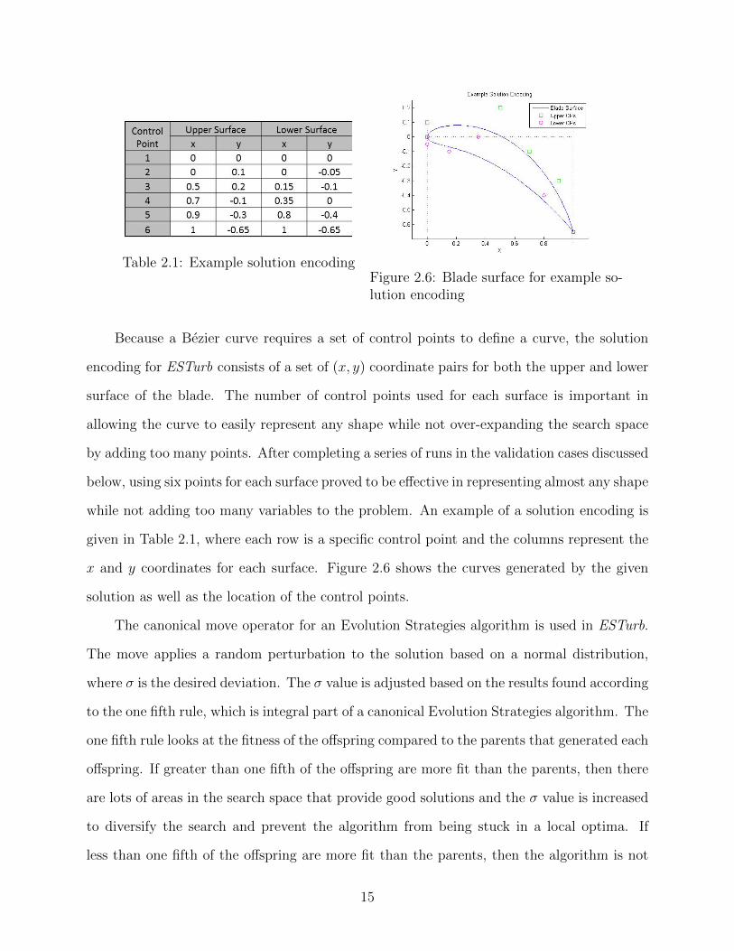
Table 2.1: Example solution encodingFigure 2.6: Blade surface for example so-lution encoding
Because a Bezier curve requires a set of control points to define a curve, the solution
encoding for ESTurb consists of a set of (x, y) coordinate pairs for both the upper and lower
surface of the blade. The number of control points used for each surface is important in
allowing the curve to easily represent any shape while not over-expanding the search space
by adding too many points. After completing a series of runs in the validation cases discussed
below, using six points for each surface proved to be effective in representing almost any shape
while not adding too many variables to the problem. An example of a solution encoding is
given in Table 2.1, where each row is a specific control point and the columns represent the
x and y coordinates for each surface. Figure 2.6 shows the curves generated by the given
solution as well as the location of the control points.
The canonical move operator for an Evolution Strategies algorithm is used in ESTurb.
The move applies a random perturbation to the solution based on a normal distribution,
where σ is the desired deviation. The σ value is adjusted based on the results found according
to the one fifth rule, which is integral part of a canonical Evolution Strategies algorithm. The
one fifth rule looks at the fitness of the offspring compared to the parents that generated each
offspring. If greater than one fifth of the offspring are more fit than the parents, then there
are lots of areas in the search space that provide good solutions and the σ value is increased
to diversify the search and prevent the algorithm from being stuck in a local optima. If
less than one fifth of the offspring are more fit than the parents, then the algorithm is not
15
finding a lot of good solutions and the σ value is decreased to intensify the search. This
typically happens when the algorithm finds a solution near the global minimum. To decrease
the value of σ it is typically multiplied by 0.85, and σ is divided by 0.85 for an increase.
A method of preventing stagnation, which will be referred to as “σ restart,” is also used in
ESTurb. Stagnation may occur if the value of σ becomes so small that it has no effect on
the solution, and if this occurs the subsequent generations will not improve results. If the
value of σ drops below some predetermined level, “σ restart” will reset the value of σ to the
initial value or some other designated number. This method works well in problems where
the solution space is not a smooth gradient and there may be many local optima that are
close in vicinity and fitness to the global optimum.
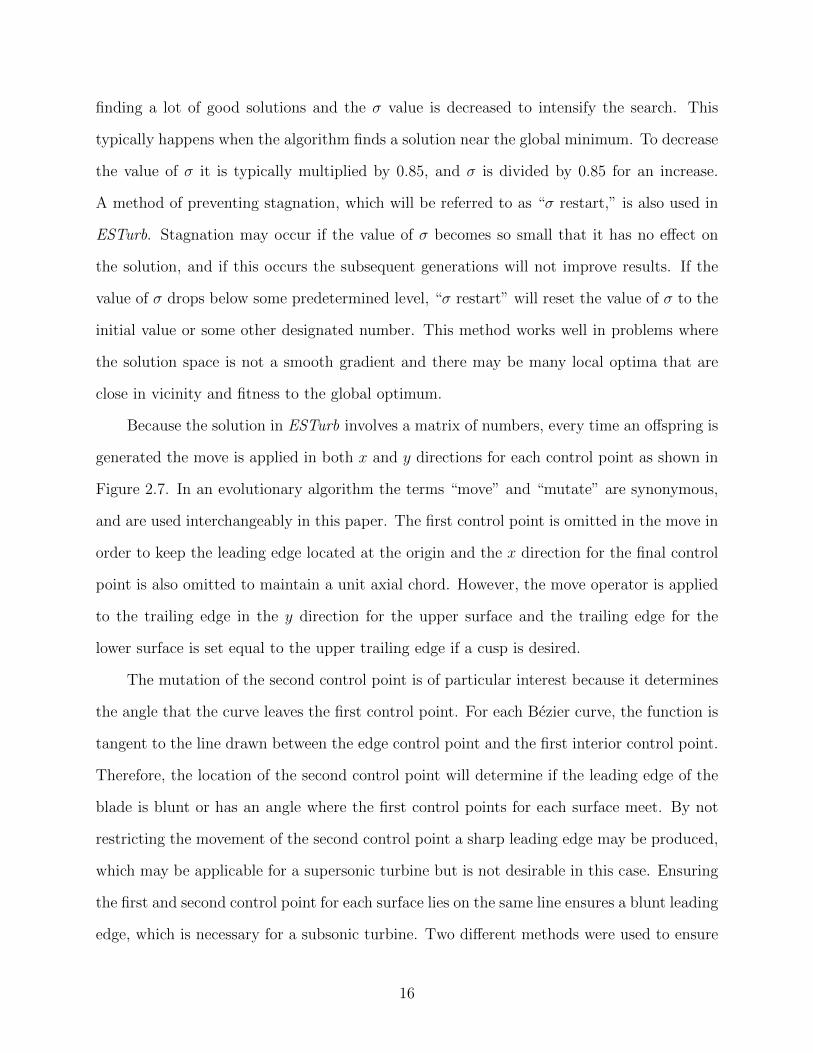
Because the solution in ESTurb involves a matrix of numbers, every time an offspring is
generated the move is applied in both x and y directions for each control point as shown in
Figure 2.7. In an evolutionary algorithm the terms “move” and “mutate” are synonymous,
and are used interchangeably in this paper. The first control point is omitted in the move in
order to keep the leading edge located at the origin and the x direction for the final control
point is also omitted to maintain a unit axial chord. However, the move operator is applied
to the trailing edge in the y direction for the upper surface and the trailing edge for the
lower surface is set equal to the upper trailing edge if a cusp is desired.
The mutation of the second control point is of particular interest because it determines
the angle that the curve leaves the first control point. For each Bezier curve, the function is
tangent to the line drawn between the edge control point and the first interior control point.
Therefore, the location of the second control point will determine if the leading edge of the
blade is blunt or has an angle where the first control points for each surface meet. By not
restricting the movement of the second control point a sharp leading edge may be produced,
which may be applicable for a supersonic turbine but is not desirable in this case. Ensuring
the first and second control point for each surface lies on the same line ensures a blunt leading
edge, which is necessary for a subsonic turbine. Two different methods were used to ensure
16

Figure 2.7: Move operator example for a single control point
a blunt leading edge on the blade, the first ensuring the flow is perpendicular to the flow
at the location of the leading control points, and the other method simply ensures the first
two control points for each surface lie on the same line. The first method is accomplished by
setting the x value of the second control point on each surface (CP2,lower &CP2,upper) to zero
and not allowing the second control point to mutate in the x direction. This ensures the
curves going into the first control points (CP1,lower & CP1,upper) are vertical, and therefore
a smooth leading edge is obtained. The second method allows CP2,upper to mutate freely.
After the mutation is complete, the distance between (CP2,lower and CP1,lower) is recorded
and mutated based on the current σ value. Then CP2,lower is relocated to a position on the
line including CP1,lower, CP1,upper, and CP2,upper the new mutated distance away from the
leading edge. The second method is desirable whenever the flow is not horizontal, such as
entering a turbine rotor after passing through a nozzle guide vane. The first method was
used in ESTurb for the optimizer validation cases and the inviscid turbine analysis, but was
updated to the second method prior to the viscous turbine analysis. Examples of an airfoil
leading edge using these two mutation methods are shown in Figures 2.8 and 2.9.
17

−0.15 −0.1 −0.05 0 0.05 0.1 0.15
−0.1
−0.05
0
0.05
0.1
0.15CP
2,upper
CP1,lower
and CP1,upper
CP2,lower
Figure 2.8: Second control point mutationoption 1
−0.06 −0.04 −0.02 0 0.02 0.04 0.06
−0.04
−0.02
0
0.02
0.04
0.06
CP2,upper
CP1,lower
and CP1,upper
CP2,lower
Figure 2.9: Second control point mutationoption 2
2.3 Optimizer Validation
After determining the type of optimizer to be used, along with the solution encoding
and move operator, the initial version of ESTurb was written following the canonical ES
optimizer form. In order to validate the optimizer and determine performance, two separate
test cases were performed. Each test case evaluated the optimizer performance compared to
the results in a published article. Considering the reasons Evolution Strategies was picked in
section 2.1, the algorithm is expected to conduct an efficient search outward from the seeded
solutions and should converge quickly. The algorithm should also find improved solutions
that the other solution encodings in the reference papers may not be able to represent due
to the restrictions placed on geometry due to the parameterization method. A flowchart for
ESTurb is shown in Figure 2.10.
2.3.1 Validation Case 1
The first validation case compared optimizer performance against the results published
in “Designing Airfoils using a Reference Point based Evolutionary Many-objective Particle
18
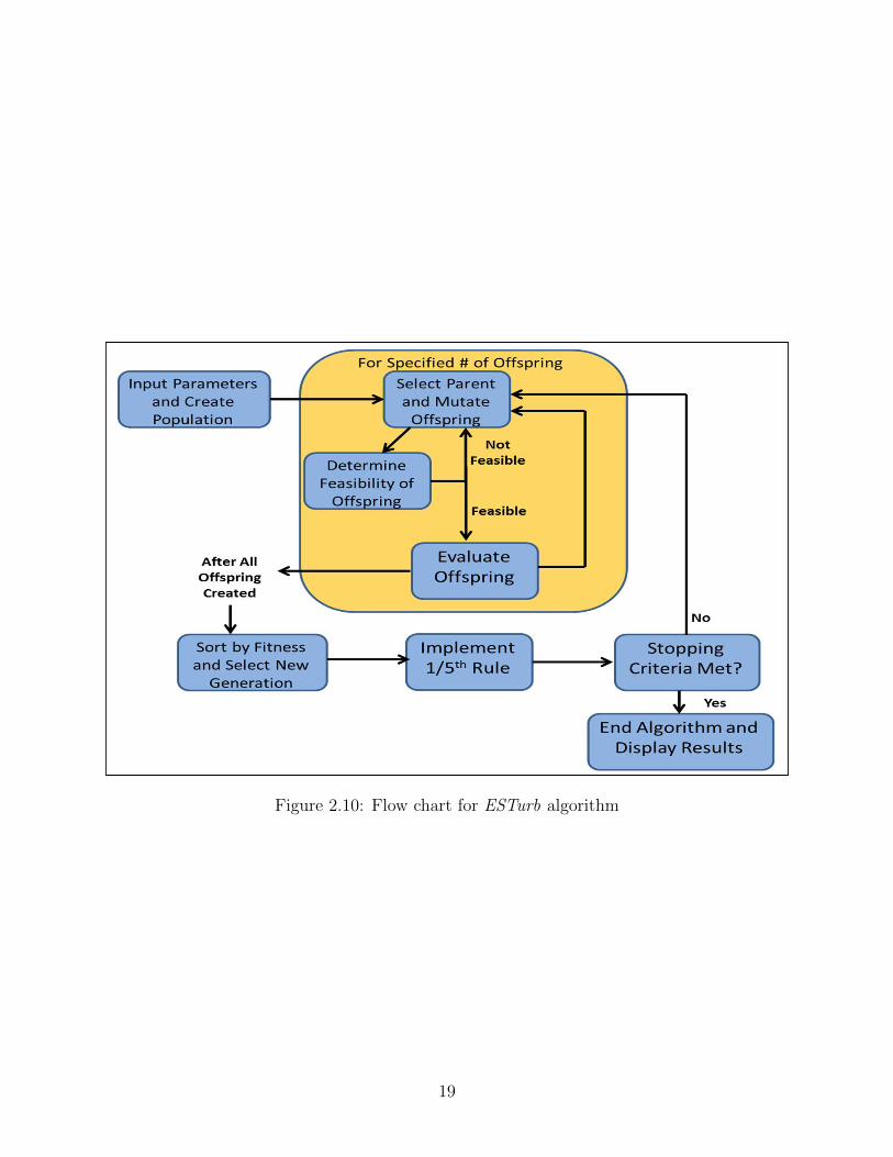
Figure 2.10: Flow chart for ESTurb algorithm
19
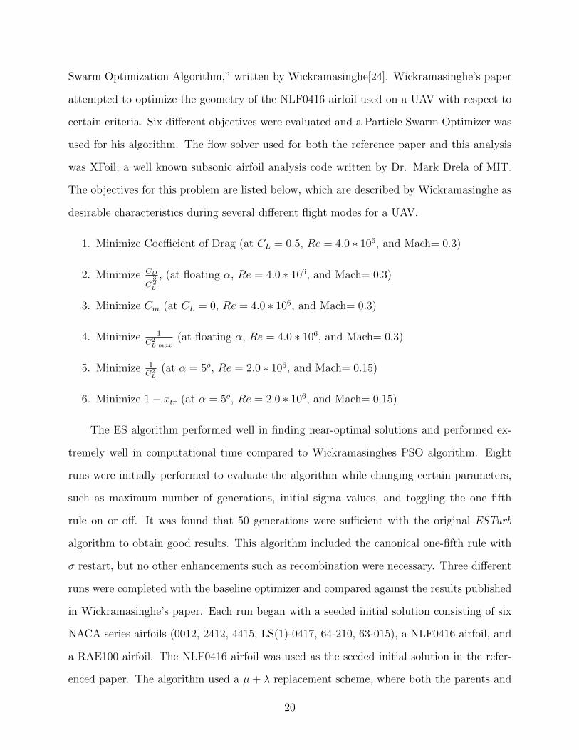
Swarm Optimization Algorithm,” written by Wickramasinghe[24]. Wickramasinghe’s paper
attempted to optimize the geometry of the NLF0416 airfoil used on a UAV with respect to
certain criteria. Six different objectives were evaluated and a Particle Swarm Optimizer was
used for his algorithm. The flow solver used for both the reference paper and this analysis
was XFoil, a well known subsonic airfoil analysis code written by Dr. Mark Drela of MIT.
The objectives for this problem are listed below, which are described by Wickramasinghe as
desirable characteristics during several different flight modes for a UAV.
1. Minimize Coefficient of Drag (at CL = 0.5, Re = 4.0 ∗ 106, and Mach= 0.3)
2. Minimize CD
C32L
, (at floating α, Re = 4.0 ∗ 106, and Mach= 0.3)
3. Minimize Cm (at CL = 0, Re = 4.0 ∗ 106, and Mach= 0.3)
4. Minimize 1C2L,max
(at floating α, Re = 4.0 ∗ 106, and Mach= 0.3)
5. Minimize 1C2L
(at α = 5o, Re = 2.0 ∗ 106, and Mach= 0.15)
6. Minimize 1− xtr (at α = 5o, Re = 2.0 ∗ 106, and Mach= 0.15)
The ES algorithm performed well in finding near-optimal solutions and performed ex-
tremely well in computational time compared to Wickramasinghes PSO algorithm. Eight
runs were initially performed to evaluate the algorithm while changing certain parameters,
such as maximum number of generations, initial sigma values, and toggling the one fifth
rule on or off. It was found that 50 generations were sufficient with the original ESTurb
algorithm to obtain good results. This algorithm included the canonical one-fifth rule with
σ restart, but no other enhancements such as recombination were necessary. Three different
runs were completed with the baseline optimizer and compared against the results published
in Wickramasinghe’s paper. Each run began with a seeded initial solution consisting of six
NACA series airfoils (0012, 2412, 4415, LS(1)-0417, 64-210, 63-015), a NLF0416 airfoil, and
a RAE100 airfoil. The NLF0416 airfoil was used as the seeded initial solution in the refer-
enced paper. The algorithm used a µ + λ replacement scheme, where both the parents and
20
1 2 3 4 5 610
−3
10−2
10−1
100
Best Airfoil Objective Values
Objective Number
Obj
Fun
ctio
n V
alue
ES AirfoilReferencePSO Airfoil
Figure 2.11: Test case one objective functionresults (sought to minimize)
Figure 2.12: Test case one computationtime comparison
offspring were considered for selection into the next generation. Five offspring were gener-
ated per parent in each generation, which resulted in 40 function evaluations per generation
and 2000 function evaluations across 50 generations.
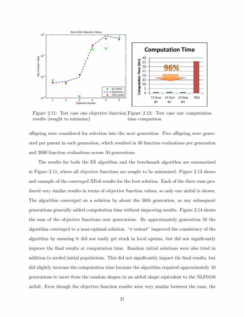
The results for both the ES algorithm and the benchmark algorithm are summarized
in Figure 2.11, where all objective functions are sought to be minimized. Figure 2.13 shows
and example of the converged XFoil results for the best solution. Each of the three runs pro-
duced very similar results in terms of objective function values, so only one airfoil is shown.
The algorithm converged on a solution by about the 50th generation, so any subsequent
generations generally added computation time without improving results. Figure 2.14 shows
the sum of the objective functions over generations. By approximately generation 50 the
algorithm converged to a near-optimal solution. “σ restart” improved the consistency of the
algorithm by ensuring it did not easily get stuck in local optima, but did not significantly
improve the final results or computation time. Random initial solutions were also tried in
addition to seeded initial populations. This did not significantly impact the final results, but
did slightly increase the computation time because the algorithm required approximately 10
generations to move from the random shapes to an airfoil shape equivalent to the NLF0416
airfoil. Even though the objective function results were very similar between the runs, the
21

Figure 2.13: XFoil output for converged airfoil
airfoil geometry was noticeably different in some of the runs. An example airfoil geometry
from another run is shown in Figure 2.15.
The computation time required for the algorithm was very reasonable considering the
large computational cost of the flow solver. The fastest run consisting of 50 generations,
which also produced the best objective function values, had a run time of 1.11 hours. All
computations were performed in Matlab on a 2.0 GHz dual-core processor. The PSO algo-
rithm required approximately 36 hours to run on a 2.3 GHz dual-core processor. Because
the XFoil flow solver accounted for over 80% of the computational time per run, the main
difference in computation time between the ES and PSO algorithms came from the number
of function evaluations required. The PSO algorithm required 10,000 function evaluations
22

Figure 2.14: History of objective function value over generations for initial eight runs
Figure 2.15: Example of variation in final population from Figure 2.13
23

while the ES algorithm required about 2,000. The use of a Hyper-Volume method for eval-
uating multiple objectives rather than using a linear combination of the objective functions
also increased time for the PSO algorithm.
2.3.2 Validation Case 2
The second paper selected for comparison is “Multi-Objective Evolutionary Optimiza-
tion of Subsonic Airfoils by Meta-Modeling and Evolution Control, written by D’Angelo[25].
In this paper a multi-objective optimization is performed using a Pareto Front to minimize
the coefficient of drag and maximize the coefficient of lift. This paper also includes work
in meta-modeling, artificial neural networks, and evolution control, but the comparison will
focus on the solution encoding and results. For problem two, the ES algorithm was generally
unchanged with the exception of adding a Pareto archive instead of a parent population, and
the parents were selected randomly from the first rank of this Pareto archive to create off-
spring. The algorithm still used a micro-population of eight members and made no changes
to the solution encoding, move operator, or any other fundamental aspects of the algorithm.
Fifteen different runs were completed in order to gain a sufficient amount of data to evaluate
the performance. Three runs for each of the five scenarios below were completed:
1. 75 generations, 300 member archive
2. 150 generations, 300 member archive
3. 250 generations, 300 member archive
4. 150 generations, 100 member archive
5. 150 generations, 500 member archive
The data from these runs is too much to display in one figure, but in general the
larger archives performed better with no change in computation time. Obviously, more
generations led to better results, but in general returns diminished substantially after about
24
150 generations. There was no single run that dominated the other runs when comparing
Pareto fronts, but the run with 150 generations and a 500 member archive performed well
and will be used as the primary comparison against D’Angelo’s results.
Figure 2.16 shows the results from D’Angelo, both using a five parameter airfoil rep-
resentation and a seven parameter representation. Each representation used two Bezier
curves, but instead of defining the airfoil geometry the curves defined the mean camber line
and airfoil thickness. The number of parameters is the number of Bezier control points used.
D’Angelo’s best result using the five parameter representation was selected for comparison,
as well as the seven parameter result utilizing Bayesian learning, which performed signifi-
cantly better. The ES results for 150 generations and a 300 member archive achieved much
better results in terms of the Pareto Front. Although not shown, each of the remaining 15
runs dominated at least a portion of the seven parameter Pareto front, and all but three of
the runs completely dominated the five parameter Pareto front from D’Angelo. The three
remaining runs dominated a majority of the five parameter front, but did not dominate the
whole front.
The five parameter model from D’Angelo required approximately two hours to complete
using just XFoil for a flow solver on a Pentium IV 2.8 GHz processor. The computational time
for the seven parameter model was not stated, but it can be assumed with the higher degrees
of freedom that the algorithm required at least as long as the five parameter model. The
ES algorithm required approximately one hour to complete 50 generations, which resulted
in a total computation time of 2.98 hours for the 150 generation, 300 member archive run.
However, even though the entire algorithm required more time to complete, the Pareto front
surpassed the five parameter front in approximately 18 minutes and dominated the seven
parameter front in approximately 25 minutes, as shown in Figure 2.17.
25

0.004 0.006 0.008 0.01 0.012 0.014 0.016 0.018 0.020.5
1
1.5
2
2.5
3Pareto Front
Cd
Cl
DAngelo 5 ParDAngelo 7 ParES Front
Figure 2.16: Pareto front results
2.3.3 Conclusions From Optimizer Validation
Both test cases proved that ESTurb is both efficient and effective at solving aerodynamic
optimization problems. By evaluating the strengths and weaknesses of different adaptive op-
timization methods, an ES algorithm was expected to converge on the optimal solution faster
than GA or PSO algorithms due to the move operator. The use of Bezier curves for the
solution encoding was expected to allow the algorithm to better represent an aerodynamic
shape, and possibly find better results that other parameterization methods could not rep-
resent. Although using Bezier curves would increase the size of the search space, the move
operator in the ES algorithm was expected to be effective enough to still allow an efficient
search with decreased computation time.
As seen in both test cases, the computation time was drastically reduced. This was
mainly due to a reduction in the number of function evaluations since the cost of each
was extremely high. The increased efficiency in the search allowed the number of function
evaluations to be greatly reduced while still maintaining comparable or better results. In
test case two especially, the ES algorithm well outperformed D’Angelo’s algorithm, finding
26

0.004 0.006 0.008 0.01 0.012 0.014 0.016 0.018 0.02
1
1.5
2
2.5
3Pareto Front vs. Computation Time
Cd
Cl
DAngelo 5 Par.DAngelo 7 Par.Initial Seeds8.73 min17.6 min24.7 min1.06 hrs1.95 hrs2.96 hrs
Figure 2.17: Pareto front progression with computation time
a Pareto front that was well in front of his best results. This validation shows that ESTurb
has the potential to be very effective for turbine optimization, and the drastic reduction in
computation time will be even more prominent as the cost of function evaluations go up,
especially when using an inviscid or viscous CFD analysis code. Additional details on each
validation case may be found in a previous article by the author[26], including algorithm
parameters used, a more detailed discussion on evolutionary computation, and algorithm
sensitivity to parameter values.
27
Chapter 3
Turbine Aerodynamic Optimization
3.1 Turbine Fundamentals Review
This paper will not spend an extensive amount of time on turbine fundamentals since
a number of great books have been written that discuss this topic in a much more detailed
and eloquent way[4][2][3]. This section will focus on reviewing the relevant aspects of turbine
fundamentals that are applicable to the optimization process used in this paper. It is assumed
that the reader is familiar with the conservation of mass, momentum and energy equations,
as well as the equation of state and the second law of thermodynamics.
The basic principle behind the turbine section in a gas turbine engine is to extract
useful power from the thermal energy in the gas leaving the combustor. A turboshaft engine
normally has a gas generator turbine (GGT) and a power turbine (PT), and each may
consist of one or more stages. The GGT is almost always the high pressure turbine directly
downstream of the combustor and it extracts power in order to drive the compressor. The
PT extracts power from the remaining thermal energy to drive the main transmission or
other components. Turbofan and turboprop engines operate in the same manner, except the
PT shaft is connected to the fan or propeller either directly or through a gearbox.
Each stage in a turbine section consists of a stator, sometimes referred to as a Nozzle
Guide Vane (NGV), and a rotor. The stator is stationary with respect to the frame and
imparts a angular momentum in the fluid with minimal losses. The rotor is rotating with an
angular velocity equal to the shaft speed and the product of the pressure force on the blade
and the angular momentum of the rotor disk result in shaft power. By applying Newton’s
2nd law the pressure force on the blade equals the net momentum change in the fluid, and
this premise leads to the well known Euler Turbine Equation (Eqn. 3.1)
28
Power = ωm(rinCθ,in − rexCθ,ex) (3.1)
The Euler Turbine Equation will be the basis for the rotor objective functions to increase
shaft power. The other major component that will be used is efficiency. There are several
different means of assessing turbine performance, including total-to-total efficiency, total-
to-static efficiency, polytropic efficiency, kinetic energy loss coefficient, total pressure loss
coefficient, entropy based efficiency, and others. Polytropic efficiency is commonly used
because it is a means of relating engines with different compressor ratios, but because we
are only concerned with one engine this is not necessary. The total-to-total (t− t) efficiency
is sufficient for all but the last stage, where the thermal energy at exit is expected to be
used. For the last stage, where any exit swirl or other thermal energy will be wasted, the
total-to-static (t − s) efficiency must be used. Note that the only difference between the
total-to-total and total-to-static efficiencies is using the static exit pressure rather than the
total exit pressure in the denominator. The total pressure loss coefficient provides a good
measure of the efficiency of a stator, where there is no work being done, and is shown in
Equation 3.4.
ηt−t =1− T0,ex
T0,in
1−(P0,ex
P0,in
) γ−1γ
(3.2)
ηt−s =1− T0,ex
T0,in
1−(Ps,exP0,in
) γ−1γ
(3.3)
ω =∆P0
P0,in
= 1− P0,ex
P0,in
(3.4)
29

3.2 Preliminary Inviscid Analysis
The purpose of the inviscid analysis is to investigate the potential for ESTurb to conduct
optimization for turbomachinery. ESTurb performed very well for simple airfoil optimiza-
tions, but it important to apply the concepts of turbine thermodynamics to an objective
function in as simple a manner as possible. Therefore, an inviscid analysis was completed
to adapt the algorithm to using a CFD code and test the new objective functions prior
to adding complications such as turbulence and heat transfer. Another main focus of the
inviscid analysis is to determine the effectiveness of using Bezier curves for turbine solution
encoding compared to other conventional blade parameterization methods. This analysis
is much easier to complete using the less costly inviscid CFD code rather than the full
Navier-Stokes CFD analysis.
3.2.1 Model and Assumptions
The application of ESTurb is very modular, so applying it to a turbine problem is as
simple as switching out the evaluation subroutine with a new one. The evaluation subroutine
can be viewed as a “black box”, receiving the solution encoding for a particular offspring as
input and producing an objective function value as output. The remainder of the ESTurb
algorithm remains the same. Because this will only involve a single objective function, the
ESTurb version used for validation case one will be used for all turbine problems. Because a
CFD code is used as the flow solver, the evaluation subroutine consists of receiving the input,
generating a grid, running the CFD code, extracting the results, and calculating the objective
function. An in-house Euler CFD code written by the author was used for this portion of
the analysis. The flow is assumed to be inviscid and the blades evaluated are assumed to
be stationary. A distance of a half chord was used both upstream and downstream of the
blade limits and the cascade was linear. There were also no structural requirements for this
analysis, only aerodynamics were considered in the objective function.
30
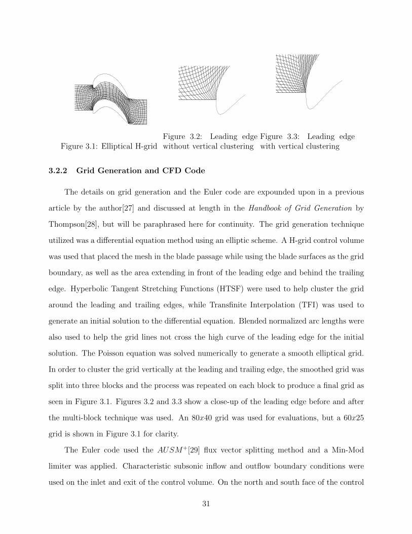
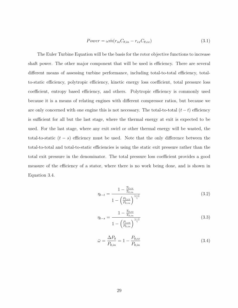
Figure 3.1: Elliptical H-gridFigure 3.2: Leading edgewithout vertical clustering
Figure 3.3: Leading edgewith vertical clustering
3.2.2 Grid Generation and CFD Code
The details on grid generation and the Euler code are expounded upon in a previous
article by the author[27] and discussed at length in the Handbook of Grid Generation by
Thompson[28], but will be paraphrased here for continuity. The grid generation technique
utilized was a differential equation method using an elliptic scheme. A H-grid control volume
was used that placed the mesh in the blade passage while using the blade surfaces as the grid
boundary, as well as the area extending in front of the leading edge and behind the trailing
edge. Hyperbolic Tangent Stretching Functions (HTSF) were used to help cluster the grid
around the leading and trailing edges, while Transfinite Interpolation (TFI) was used to
generate an initial solution to the differential equation. Blended normalized arc lengths were
also used to help the grid lines not cross the high curve of the leading edge for the initial
solution. The Poisson equation was solved numerically to generate a smooth elliptical grid.
In order to cluster the grid vertically at the leading and trailing edge, the smoothed grid was
split into three blocks and the process was repeated on each block to produce a final grid as
seen in Figure 3.1. Figures 3.2 and 3.3 show a close-up of the leading edge before and after
the multi-block technique was used. An 80x40 grid was used for evaluations, but a 60x25
grid is shown in Figure 3.1 for clarity.
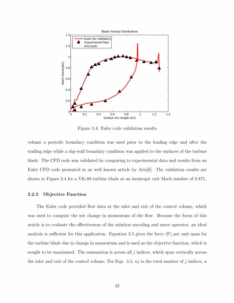
The Euler code used the AUSM+[29] flux vector splitting method and a Min-Mod
limiter was applied. Characteristic subsonic inflow and outflow boundary conditions were
used on the inlet and exit of the control volume. On the north and south face of the control
31
0 0.2 0.4 0.6 0.8 1 1.2 1.40
0.2
0.4
0.6
0.8
1
1.2
1.4Blade Velocity Distributions
Surface Arc−length (s/c)
Mac
h (is
entr
opic
)
Euler (for validation)Experimental DataArts Euler
Figure 3.4: Euler code validation results
volume a periodic boundary condition was used prior to the leading edge and after the
trailing edge while a slip-wall boundary condition was applied to the surfaces of the turbine
blade. The CFD code was validated by comparing to experimental data and results from an
Euler CFD code presented in an well known article by Arts[6]. The validation results are
shown in Figure 3.4 for a VK-89 turbine blade at an isentropic exit Mach number of 0.875.
3.2.3 Objective Function
The Euler code provided flow data at the inlet and exit of the control volume, which
was used to compute the net change in momentum of the flow. Because the focus of this
article is to evaluate the effectiveness of the solution encoding and move operator, an ideal
analysis is sufficient for this application. Equation 3.5 gives the force (F) per unit span for
the turbine blade due to change in momentum and is used as the objective function, which is
sought to be maximized. The summation is across all j indices, which span vertically across
the inlet and exit of the control volume. For Eqn. 3.5, nj is the total number of j indices, u
32

and v represent the horizontal and vertical fluid velocities respectively, and l represents the
vertical cell height.
F =
nj∑j=1
ρin,j(uin,jlin,j)vin,j −nj∑j=1
ρex,j(uex,jlex,j)vex,j (3.5)
Because grid generation and CFD codes can sometimes fail to converge properly, a few
safeguards were put in place to ensure ESTurb did not fail altogether. First, the solution
was checked after mutation to ensure the upper and lower surfaces did not cross and the
offspring was feasible. If either the grid generation code or the CFD code failed or did not
converge properly an output file would not be created. A simple timer was started when the
evaluation began, and if the timer expired without an output file present the solution would
be assigned an objective function value of zero and the optimizer would move on to the next
offspring. Convergence failures were fairly uncommon and did not impact the algorithm’s
ability to converge on a solution.
3.2.4 Results and Optimizer Performance
In order to evaluate the ability of the algorithm to optimize turbine blade geometry
and the effectiveness of the solution encoding, runs were completed using the Bezier curve
encoding as well as the spline-connected polynomial (SCP) encoding shown in Figures 2.4
and 2.5. Each run consisted of a micro-population of 4 members and a λ/µ (offspring to
parent) ratio of 4, for a total of 16 offspring per generation. As in the validation cases, 50
generations were evaluated and the standard deviation, σ, was initially set to 0.03 with the
one-fifth rule and “σ restart” included. Initial solutions were seeded, the inflow angle was
set to 30o, and the exit isentropic Mach number was set to 0.875. In order to set the throat
distance a desired throat was entered and a bisection method was used to adjust the pitch
until the correct throat was obtained. The throat in turbine design is the minimum distance,
or area for three-dimensions, between blades. The throat is not necessarily choked, but this
is often the case for one or more stages in a turbine near design operating conditions. The
33
trailing edge of the turbine blades is cusped, and a maximum tangential chord of 1 was
allowed for feasible solutions.
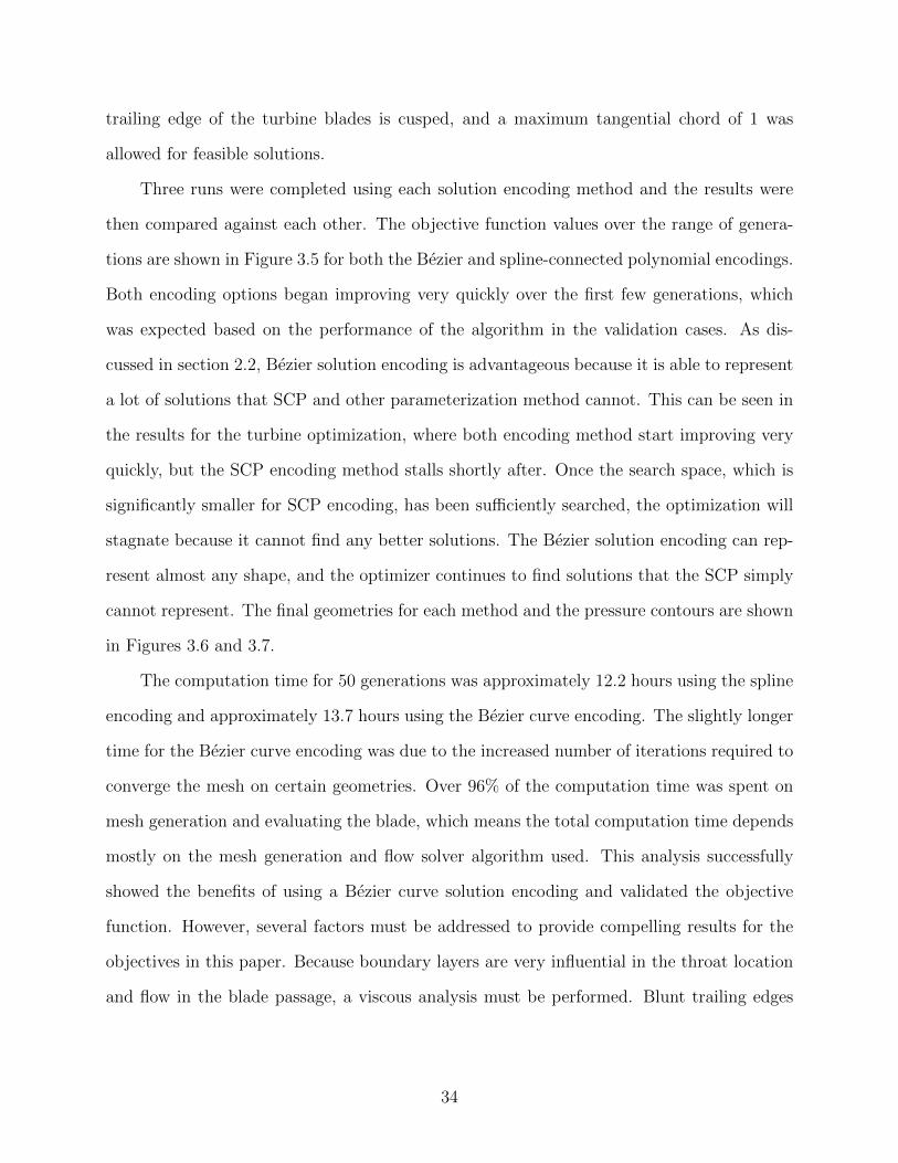
Three runs were completed using each solution encoding method and the results were
then compared against each other. The objective function values over the range of genera-
tions are shown in Figure 3.5 for both the Bezier and spline-connected polynomial encodings.
Both encoding options began improving very quickly over the first few generations, which
was expected based on the performance of the algorithm in the validation cases. As dis-
cussed in section 2.2, Bezier solution encoding is advantageous because it is able to represent
a lot of solutions that SCP and other parameterization method cannot. This can be seen in
the results for the turbine optimization, where both encoding method start improving very
quickly, but the SCP encoding method stalls shortly after. Once the search space, which is
significantly smaller for SCP encoding, has been sufficiently searched, the optimization will
stagnate because it cannot find any better solutions. The Bezier solution encoding can rep-
resent almost any shape, and the optimizer continues to find solutions that the SCP simply
cannot represent. The final geometries for each method and the pressure contours are shown
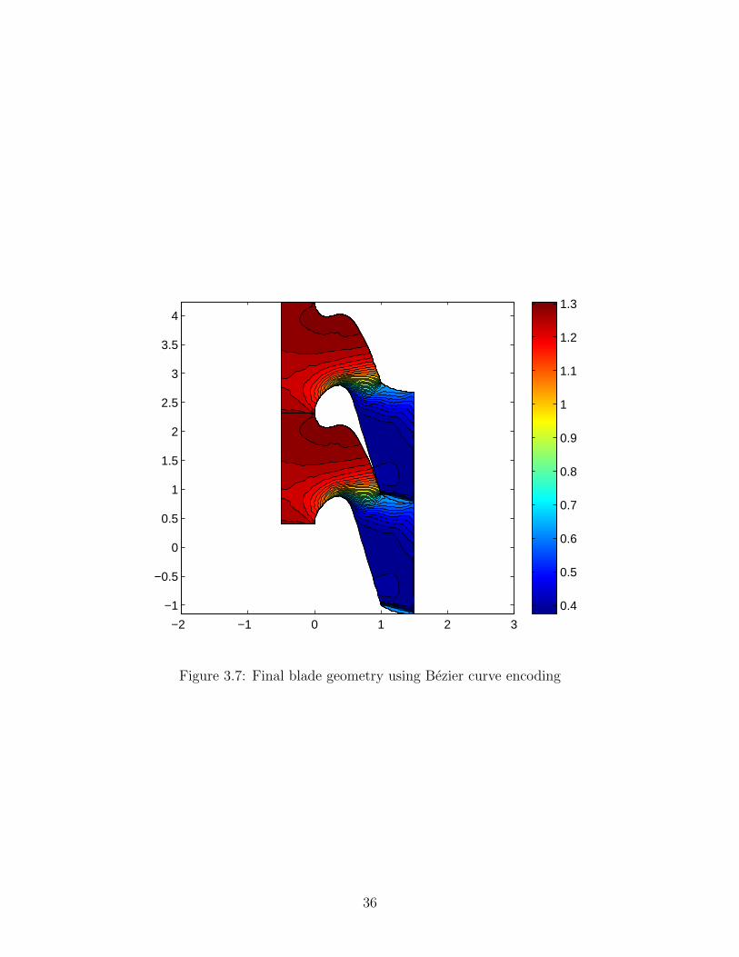
in Figures 3.6 and 3.7.
The computation time for 50 generations was approximately 12.2 hours using the spline
encoding and approximately 13.7 hours using the Bezier curve encoding. The slightly longer
time for the Bezier curve encoding was due to the increased number of iterations required to
converge the mesh on certain geometries. Over 96% of the computation time was spent on
mesh generation and evaluating the blade, which means the total computation time depends
mostly on the mesh generation and flow solver algorithm used. This analysis successfully
showed the benefits of using a Bezier curve solution encoding and validated the objective
function. However, several factors must be addressed to provide compelling results for the
objectives in this paper. Because boundary layers are very influential in the throat location
and flow in the blade passage, a viscous analysis must be performed. Blunt trailing edges
34

0 10 20 30 40 500.35
0.4
0.45
0.5
0.55
0.6
0.65
0.7
Generation
Obj
Fun
ctio
n V
alue
Obj Function vs. Generation
Spline Run 1Spline Run 2Spline Run 3Bezier Run 1Bezier Run 2Bezier Run 3
Figure 3.5: Objective function values over 50 generations
−1.5 −1 −0.5 0 0.5 1 1.5 2 2.5
0
0.5
1
1.5
2
2.5
3
0.4
0.5
0.6
0.7
0.8
0.9
1
1.1
1.2
Figure 3.6: Final blade geometry using spline-connected polynomial encoding
35
−2 −1 0 1 2 3
−1
−0.5
0
0.5
1
1.5
2
2.5
3
3.5
4
0.4
0.5
0.6
0.7
0.8
0.9
1
1.1
1.2
1.3
Figure 3.7: Final blade geometry using Bezier curve encoding
36
and simple structural requirements must also be included. These will be discussed in the
next section.
3.3 Viscous Turbine Analysis
The viscous analysis will provide a much more thorough evaluation of the turbine blades,
including boundary layer effects, flow separation, and frictional losses. This higher fidelity
analysis also comes with a computational cost, especially when a large number of iterations
are required. Because the application of a Navier-Stokes analysis requires a much greater
amount of expertise and is outside the scope of this paper, two codes generated by NASA were
used. The grid generation code was replaced with GRAPE, a well known grid generation
software also based on solving Poisson’s equation that was written by Reece Sorenson at
NASA Ames Research Center and was modified by Dr. Rodrick Chima. This code follows
the same methodology as the code written by the author, but is much more user friendly
and robust. GRAPE allows the use of a “C”, “O”, or “H” grid topology, but the C-grid will
be used for this application because it works well with the Navier-Stokes code.
The CFD code used is Rotor Viscous Code Quasi-Three Dimensional (RVCQ3D), which
was written by Dr. Rodrick Chima at NASA Glenn Research Center. Both GRAPE and
RVCQ3D are available on the NASA Glenn Research Center Software Repository. RVCQ3D
is a code specifically developed for turbomachinery that solves the thin-layer Navier-Stokes
equation on a blade-to-blade surface of revolution. It uses central or upwind finite dif-
ferencing techniques and includes three turbulence models and the ability to predict heat
transfer. The AUSM+ upwind differencing scheme was used for this analysis along with the
low Reynold’s number Wilcox k−ω turbulence model. An explicit multistage Runge-Kutta
scheme is used with local time-stepping and the flow variables are non-dimensionalized us-
ing freestream conditions. Multiple articles have been written by Dr. Chima[9][10][11][12]
validating the results of RVCQ3D with experimental data for each of the turbulence models
as well as heat transfer predictions. These articles also show the sensitivity of RVCQ3D
37
to changing variables such as Reynold’s Number, eddy viscosity ratio, freestream turbu-
lence, grid refinement, and a comparison between the turbulence models. Full details on the
methodology of RVCQ3D are provided in the User’s Manual[30] and are elaborated on in
the other articles by Dr. Chima. Care was taken to check and ensure the wall grid spacing
(y+) was approximately less than 1 for each of the final solutions and the eddy viscosity
ratio was in the range used by Dr. Chima in other published articles[10]. The final grid for
each solution was also visually checked to ensure the grid spacing was adequate for the final
blade shape and spacing.
3.3.1 Model and Assumptions
The viscous model accounts for frictional losses through the use of the k−ω turbulence
model, and uses an updated non-reflecting boundary condition for inlet and exit as well as
an updated no-slip boundary condition on the turbine blade wall. The analysis is Quasi-3-D,
taking into account the stream tube geometry from the T55 mean radial path, but does not
include any losses specific to full 3D analysis such as tip leakage. RVCQ3D also allowed
the rotational velocity of the turbine blades to be entered for rotors, while the stator blades
were kept stationary. The numerical parameters recommended in the User’s Manual for the
most robust scheme were used, including a Courant number of 2.5. Example input files for
RVCQ3D are given in Appendix B.
The grid used for the analysis was 169x45, which has been shown by several articles
to be sufficient for this type of analysis[31] and verified by testing a variety of grids up to
383x55 with no significant change in the results. Grid parameters recommended by the
RVCQ3D User’s Manual for heat transfer applications were used, including a grid spacing of
a hundredth of a chord around the trailing edge and four hundredths of a chord around the
leading edge. For a unit axial chord, the grid height at the blade surface was 1.0∗10−5. The
remainder of the input parameters are listed in the example GRAPE input file in Appendix
38
B. An example 169x45 grid for a VK-LS89 turbine blade as described in Arts[6] is shown in
Figure 3.8.
Stator/rotor interactions are very difficult to model, and an unsteady solution is neces-
sary to capture the effects of the pressure fluctuations as the rotor blades interact with the
stator wakes. RVCQ3D is a single-block steady state code, which limits the accuracy of the
stator/rotor interaction considerably. The analysis was completed in the direction of flow
using the pressure ratios from the T55 design report, and the energy averaged flow properties
at the stator exit were used for the inlet conditions of the rotor. This analysis is rudimen-
tary at best, but will be sufficient in determining the effectiveness of ESTurb for turbine
optimization. If ESTurb is shown effective in turbine optimization, a higher fidelity analysis
using a multi-block code such as SWIFT would allow a more accurate model of a stage or
multi-stage analysis. A multi-block code would evaluate all stages at once by transferring
properties between blade rows at grid interfaces as described in Calculation of Multistage
Turbomachinery Using Steady Characteristic Boundary Conditions by Dr. Chima[32].
3.3.2 Optimizer Updates and Objective Function
In order to incorporate GRAPE and RVCQ3D the evaluation subroutine was updated
again, but the remainder of the ESTurb code remained the same. The evaluation subroutine
consisted of accepting inputs from the main program, writing input files and executing
GRAPE and RVCQ3D, extracting data from the output files, and calculating the objective
function. As in the inviscid case, if either of the executables failed the objective function
would be set to zero and the algorithm would move on to the next offspring.
The objective function was refined to included the losses calculated by the turbulence
model. The objective function used for stators was as combination of the fluid tangential
momentum change and the ratio of P0,2/P0,1, which is also equal to (1 − ω). Because the
fluid mass flow rate varied slightly due to stream tube thickness and other factors, only
the difference in fluid tangential velocity was considered for the momentum change. The
39

X
Y
0 1 2
-3.5
Figure 3.8: Example 169x45 grid for VK-LS89 turbine blade40

X
Y
2.03 2.04 2.05 2.06 2.07 2.08 2.09
-0.73
-0.72
-0.71
-0.7
-0.69
-0.68
Figure 3.9: Close-up of trailing edge for VK-LS89 turbine blade grid
41
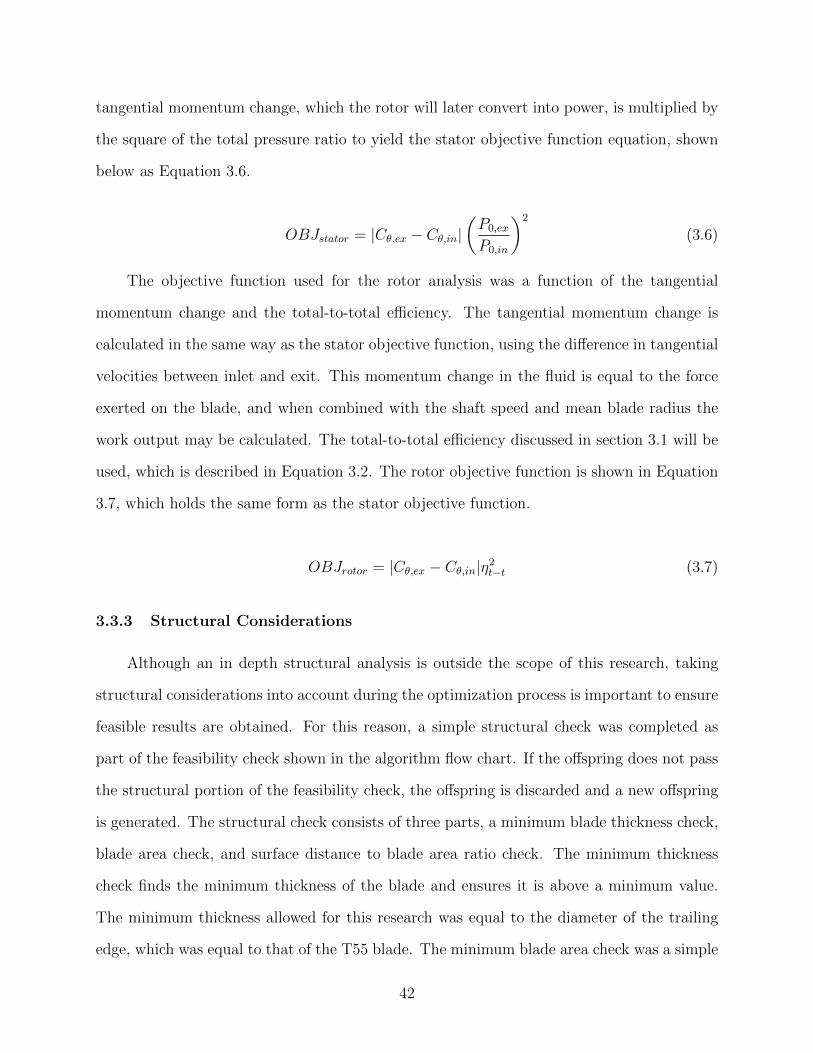
tangential momentum change, which the rotor will later convert into power, is multiplied by
the square of the total pressure ratio to yield the stator objective function equation, shown
below as Equation 3.6.
OBJstator = |Cθ,ex − Cθ,in|(P0,ex
P0,in
)2
(3.6)
The objective function used for the rotor analysis was a function of the tangential
momentum change and the total-to-total efficiency. The tangential momentum change is
calculated in the same way as the stator objective function, using the difference in tangential
velocities between inlet and exit. This momentum change in the fluid is equal to the force
exerted on the blade, and when combined with the shaft speed and mean blade radius the
work output may be calculated. The total-to-total efficiency discussed in section 3.1 will be
used, which is described in Equation 3.2. The rotor objective function is shown in Equation
3.7, which holds the same form as the stator objective function.
OBJrotor = |Cθ,ex − Cθ,in|η2t−t (3.7)
3.3.3 Structural Considerations
Although an in depth structural analysis is outside the scope of this research, taking
structural considerations into account during the optimization process is important to ensure
feasible results are obtained. For this reason, a simple structural check was completed as
part of the feasibility check shown in the algorithm flow chart. If the offspring does not pass
the structural portion of the feasibility check, the offspring is discarded and a new offspring
is generated. The structural check consists of three parts, a minimum blade thickness check,
blade area check, and surface distance to blade area ratio check. The minimum thickness
check finds the minimum thickness of the blade and ensures it is above a minimum value.
The minimum thickness allowed for this research was equal to the diameter of the trailing
edge, which was equal to that of the T55 blade. The minimum blade area check was a simple
42

way to ensure the blade could withstand the stress of the pressure and inertial forces on the
blade and ensured the optimized blade area was no less than the area of the T55 blade minus
a 10% buffer. The last check measured the ratio of the surface distance to the blade area.
This check was not only for structural purposes, but during the aerothermal optimization
this was a simple way of keeping the ratio from increasing to a point where the blade could
not be cooled properly. The surface to area ratio was not allowed to be more than that of the
T55 blade plus a 20% buffer. Although this check does not replace a full structural analysis,
it does provide a simple estimate of the structural feasibility of the blade and is sufficient
for the purposes of this research.
3.3.4 Results and Optimizer Performance
The single stage viscous analysis was completed using the stream tube and thermody-
namic data for the first stage of the gas generator turbine (GGT) in the T55 engine. The T55
stator and rotor blades were used for the seeded solutions in a micro-population of 4. The
λ/µ ratio was set to 2 for a total of 8 offspring per generation and 400 function evaluations
over 50 generations. The analysis required approximately 14 hours to complete per blade
row on a 2.0 GHz dual core processor, for a total of 28 hours for the entire stage. The stator
was optimized first over 50 generations using the inlet conditions and exit static pressure in
the T55. The energy averaged flow variables at stator exit were used as the inlet conditions
for the rotor analysis along with the rotor exit static pressure and the blade angular velocity
from the T55 design report. The rotor optimization process was also 50 generations. As
discussed earlier, all results compared to the original T55 engine will be given in percentages
to protect the proprietary information.
The optimized geometry and pressure contours for the first stage are given in Figure
3.10. Blanking variables are used to omit the overlapped region between the blades in
Figure 3.10 even though the grid extended half a chord length axially both before and after
the blade. The Mach contours for both the stator and rotor are shown separately with the
43

full computational grid in Figures 3.11 and 3.12. Note that several computational domains
were stacked in a cascade for viewing purposes, but the control volume analyzed consisted
of only one blade passage. ESTurb performed well at optimizing both the stator and rotor
in reasonable amounts of time. As expected the optimizer increased the flow angle exiting
the stator to impart more momentum into the fluid without separating the flow over the
suction surface of the stator. The rotor calculation also performed well at providing a large
momentum change with little or no turbulence. After completing two runs, the average
optimized blade geometry resulted in a 1.1% increase in isentropic efficiency and a 7.0%
increase in power output for the stage when compared to the T55. The results for the
two runs were very similar, differing by less than 0.1%, so only the geometry for the first
run is shown. The increased performance is mainly due to a greater change in tangential
momentum by the stator and the rotor, but it is important to note that the optimizer was
able to find a blade geometry that could significantly increase the momentum change while
also increasing the isentropic efficiency by over one percent. Example GRAPE and RVCQ3D
input files are included in Appendix B, but the stream tube geometry for the T55 has been
removed and must be replaced or the “nblade” and “nmn” variables must be updated for it
to run. All remaining data in the input files is non-proprietary.
44
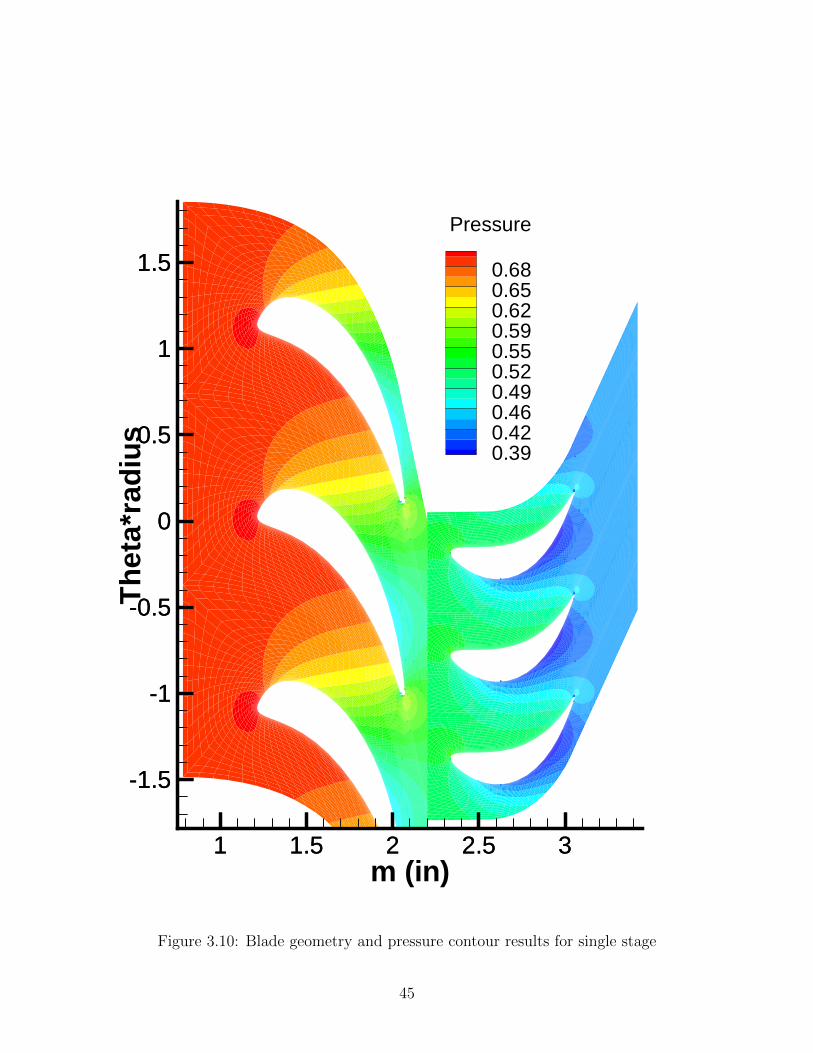
m (in)
Th
eta*
rad
ius
1 1.5 2 2.5 3
-1.5
-1
-0.5
0
0.5
1
1.5
Pressure
0.680.650.620.590.550.520.490.460.420.39
1 1.5 2 2.5 3
-1.5
-1
-0.5
0
0.5
1
1.5
Figure 3.10: Blade geometry and pressure contour results for single stage
45

X
Y
1 1.5 2 2.5 3-1.5
-1
-0.5
0
0.5Mach Number
0.80.750.70.650.60.550.50.450.40.350.30.250.20.150.10.05
Figure 3.11: Mach Number contours for stator
46
X
Y
2 2.5 3 3.5
-1.5
-1
-0.5
0 Mach Number
0.70.650.60.550.50.450.40.350.30.250.20.150.10.05
Figure 3.12: Absolute Mach Number contours for rotor
47
Chapter 4
Turbine Aerothermal Optimization
An aerothermal analysis is completed in this report in order to investigate the trade-
off between aerodynamic and thermal performance during optimization. This analysis is
completed for two primary reasons, the first being the lack of research in this area using
an adaptive optimizer. Of all the articles reviewed by the author, none could be found
that used an adaptive optimizer and evaluated both aerodynamic performance and heat
transfer. The second reason is the potential for Bezier curve blade representation to provide
optimal leading edge geometries for this problem. Of the 7 turbine design books and many
more journal articles reviewed by the author, including those listed in the literature review,
every one suggests defining the leading edge geometry of a blade using a circle or an ellipse.
Although this provides a great aerodynamic advantage and therefore is commonly used,
intuition would suggest that having a more flexible parameterization method might lead to
better designs, especially when multiple objectives are considered. This greater flexibility in
the geometry may lead to a more thermally resistant blade which would allow higher turbine
inlet temperatures. Because turbine inlet temperature is directly related to maximum power
output, this could be advantageous. The analysis conducted in this paper is assuming the
turbine blade is not cooled for simplicity purposes.
4.1 Heat Transfer Model
The heat transfer model used for this analysis is incorporated into the RVCQ3D analysis
code. The code uses the k−ω turbulence model with transition effects to predict the Stanton
Number at locations around the blade. As seen in Eqn. 4.1, a slightly adapted equation for
the Stanton Number definition from the RVCQ3D User’s Manual[30], the Stanton Number
48
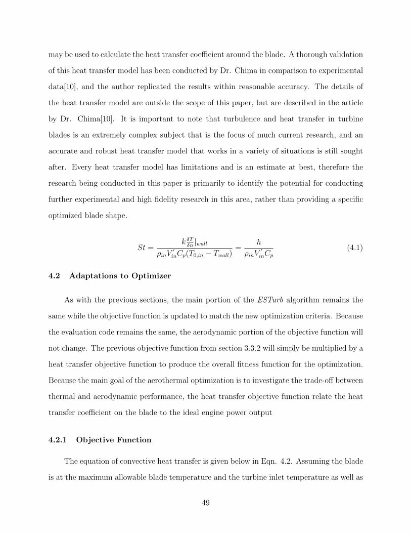
may be used to calculate the heat transfer coefficient around the blade. A thorough validation
of this heat transfer model has been conducted by Dr. Chima in comparison to experimental
data[10], and the author replicated the results within reasonable accuracy. The details of
the heat transfer model are outside the scope of this paper, but are described in the article
by Dr. Chima[10]. It is important to note that turbulence and heat transfer in turbine
blades is an extremely complex subject that is the focus of much current research, and an
accurate and robust heat transfer model that works in a variety of situations is still sought
after. Every heat transfer model has limitations and is an estimate at best, therefore the
research being conducted in this paper is primarily to identify the potential for conducting
further experimental and high fidelity research in this area, rather than providing a specific
optimized blade shape.
St =k δTδn|wall
ρinV′inCp(T0,in − Twall)
=h
ρinV′inCp
(4.1)
4.2 Adaptations to Optimizer
As with the previous sections, the main portion of the ESTurb algorithm remains the
same while the objective function is updated to match the new optimization criteria. Because
the evaluation code remains the same, the aerodynamic portion of the objective function will
not change. The previous objective function from section 3.3.2 will simply be multiplied by a
heat transfer objective function to produce the overall fitness function for the optimization.
Because the main goal of the aerothermal optimization is to investigate the trade-off between
thermal and aerodynamic performance, the heat transfer objective function relate the heat
transfer coefficient on the blade to the ideal engine power output
4.2.1 Objective Function
The equation of convective heat transfer is given below in Eqn. 4.2. Assuming the blade
is at the maximum allowable blade temperature and the turbine inlet temperature as well as
49

the heat transfer coefficient are known, the heat transfer into the blade may be calculated.
For evaluating an optimized blade it can be assumed that the heat transfer into the blade
and the blade temperature is held the same, and therefore a change in the heat transfer
coefficient will result in a change in allowable turbine inlet temperature. The new turbine
inlet temperature may then be moved to the left hand side of the equation as shown in Eqn.
4.3
q = h(T0 − Twall) (4.2)
T0,new =hnewhold
(T0,old − Twall,old) + Twall,old (4.3)
The ideal engine analysis discussed in Mattingly[1] provides a relation between a turbine
inlet temperature increase and power increase. Equation 4.4 is a simplified version of the
expression in Mattingly for shaft power from an ideal turboshaft engine. Plotting this equa-
tion over a range of compressor ratios and turbine inlet temperatures results in Figure 4.1.
If a compressor ratio is selected a linear relationship between the turbine inlet temperature
ratio and shaft power ratio may be obtained through a simple curve fit. The relationship
used for this analysis is described in Eqn. 4.5 and shown in Figure 4.2. After running the
evaluation on a blade and the peak heat transfer coefficient is obtained, Eqn. 4.3 is used to
calculate the maximum turbine inlet temperature and Eqn. 4.5 is used to obtain a ratio for
Wnew/Wold. This ratio is then multiplied with the aerodynamic objective function to obtain
an overall objective function.
Wshaft = m0CpT0
[T0,turbineT0,∞
(1− 1
πγ−1γ
c
)−(πγ−1γ
c − 1
)](4.4)
Wnew
Wold
= 1.5935T0,newT0,old
− 0.5935 (4.5)
50
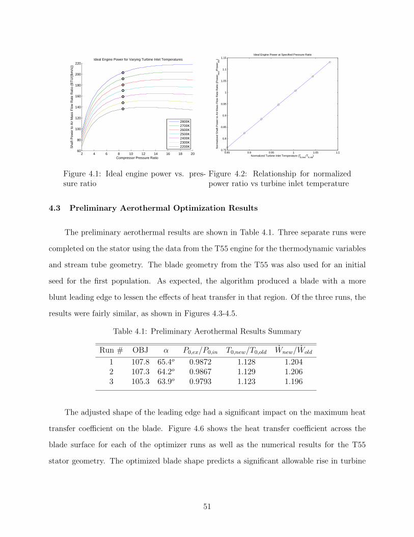
2 4 6 8 10 12 14 16 18 2060
80
100
120
140
160
180
200
220Ideal Engine Power for Varying Turbine Inlet Temperatures
Compressor Pressure Ratio
Sha
ft P
ower
to A
ir M
ass
Flo
w R
ate
Rat
io (
BT
U/(
lbm
/s))
2800K2700K2600K2500K2400K2300K2200K
Figure 4.1: Ideal engine power vs. pres-sure ratio
0.85 0.9 0.95 1 1.05 1.10.75
0.8
0.85
0.9
0.95
1
1.05
1.1
1.15Ideal Engine Power at Specified Pressure Ratio
Normalized Turbine Inlet Temperature (T0,new
/T0,old
)
Nor
mal
ized
Sha
ft P
ower
to A
ir M
ass
Flo
w R
ate
Rat
io (
Pow
erne
w/P
ower
old)
Figure 4.2: Relationship for normalizedpower ratio vs turbine inlet temperature
4.3 Preliminary Aerothermal Optimization Results
The preliminary aerothermal results are shown in Table 4.1. Three separate runs were
completed on the stator using the data from the T55 engine for the thermodynamic variables
and stream tube geometry. The blade geometry from the T55 was also used for an initial
seed for the first population. As expected, the algorithm produced a blade with a more
blunt leading edge to lessen the effects of heat transfer in that region. Of the three runs, the
results were fairly similar, as shown in Figures 4.3-4.5.
Table 4.1: Preliminary Aerothermal Results Summary
Run # OBJ α P0,ex/P0,in T0,new/T0,old Wnew/Wold
1 107.8 65.4o 0.9872 1.128 1.2042 107.3 64.2o 0.9867 1.129 1.2063 105.3 63.9o 0.9793 1.123 1.196
The adjusted shape of the leading edge had a significant impact on the maximum heat
transfer coefficient on the blade. Figure 4.6 shows the heat transfer coefficient across the
blade surface for each of the optimizer runs as well as the numerical results for the T55
stator geometry. The optimized blade shape predicts a significant allowable rise in turbine
51
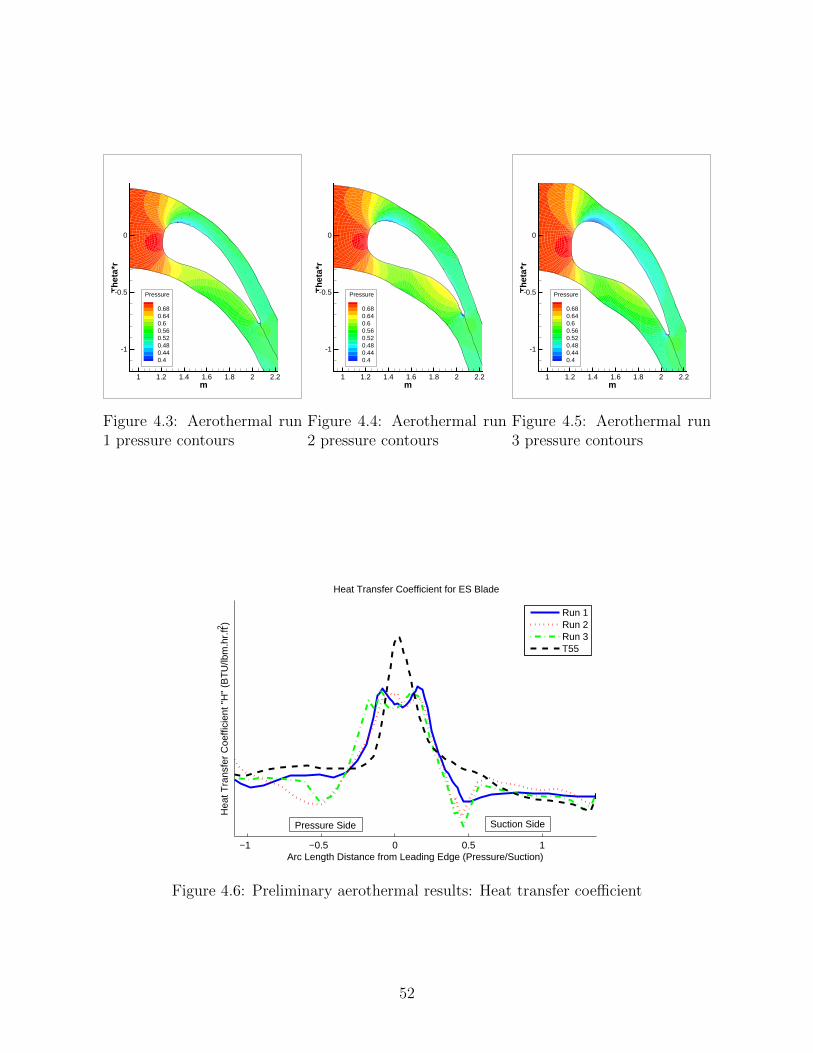
m
Th
eta*
r
1 1.2 1.4 1.6 1.8 2 2.2
-1
-0.5
0
Pressure
0.680.640.60.560.520.480.440.4
Figure 4.3: Aerothermal run1 pressure contours
m
Th
eta*
r
1 1.2 1.4 1.6 1.8 2 2.2
-1
-0.5
0
Pressure
0.680.640.60.560.520.480.440.4
Figure 4.4: Aerothermal run2 pressure contours
m
Th
eta*
r
1 1.2 1.4 1.6 1.8 2 2.2
-1
-0.5
0
Pressure
0.680.640.60.560.520.480.440.4
Figure 4.5: Aerothermal run3 pressure contours
−1 −0.5 0 0.5 1
Heat Transfer Coefficient for ES Blade
Arc Length Distance from Leading Edge (Pressure/Suction)
Hea
t Tra
nsfe
r C
oeffi
cien
t "H
" (B
TU
/lbm
.hr.
ft2 )
Run 1Run 2Run 3T55
Pressure Side Suction Side
Figure 4.6: Preliminary aerothermal results: Heat transfer coefficient
52
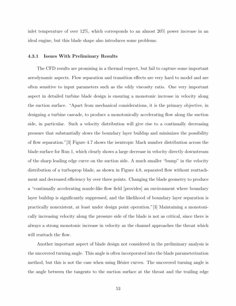
inlet temperature of over 12%, which corresponds to an almost 20% power increase in an
ideal engine, but this blade shape also introduces some problems.
4.3.1 Issues With Preliminary Results
The CFD results are promising in a thermal respect, but fail to capture some important
aerodynamic aspects. Flow separation and transition effects are very hard to model and are
often sensitive to input parameters such as the eddy viscosity ratio. One very important
aspect in detailed turbine blade design is ensuring a monotonic increase in velocity along
the suction surface. “Apart from mechanical considerations, it is the primary objective, in
designing a turbine cascade, to produce a monotonically accelerating flow along the suction
side, in particular. Such a velocity distribution will give rise to a continually decreasing
pressure that substantially slows the boundary layer buildup and minimizes the possibility
of flow separation.”[3] Figure 4.7 shows the isentropic Mach number distribution across the
blade surface for Run 1, which clearly shows a large decrease in velocity directly downstream
of the sharp leading edge curve on the suction side. A much smaller “bump” in the velocity
distribution of a turboprop blade, as shown in Figure 4.8, separated flow without reattach-
ment and decreased efficiency by over three points. Changing the blade geometry to produce
a “continually accelerating nozzle-like flow field [provides] an environment where boundary
layer buildup is significantly suppressed, and the likelihood of boundary layer separation is
practically nonexistent, at least under design point operation.”[3] Maintaining a monotoni-
cally increasing velocity along the pressure side of the blade is not as critical, since there is
always a strong monotonic increase in velocity as the channel approaches the throat which
will reattach the flow.
Another important aspect of blade design not considered in the preliminary analysis is
the uncovered turning angle. This angle is often incorporated into the blade parameterization
method, but this is not the case when using Bezier curves. The uncovered turning angle is
the angle between the tangents to the suction surface at the throat and the trailing edge
53

0 0.5 1 1.50
0.1
0.2
0.3
0.4
0.5
0.6
0.7
0.8
0.9
1
Surface Arc Length
Isen
trop
ic M
ach
Num
ber
PressureSuctionThroat Loc
Adverse Pressure Gradient
"Bump" in Velocity Distribution
Figure 4.7: Aerothermal run 1 Mach num-ber distribution
Figure 4.8: “Bump” in velocity distribu-tion for turboprop blade[3]
merging point. It is referred to as “uncovered” because the region of the blade suction
side after the throat is not confined within the blade passage. A small uncovered turning
angle facilitates accelerating flow over the suction side after the throat, which increases
performance. However, too large of an angle may have detrimental effects.
4.3.2 Updates to Objective Function
Updating the objective function to account for these two issues is easily implemented
in the form of a penalty function. After evaluating each blade in RVCQ3D, the velocity
distributions for each surface are checked. If the suction surface decreases velocity prior to
the throat location the gradient of the velocity decrease is used to produce a penalty factor
while is less than one. The penalty factor is then multiplied with the objective function
value to decrease it proportional to the severity of the diffusion on the blade. Because the
pressure side is more forgiving, a similar process is used including a buffer. If the velocity
decreases more than 15% of the exit Mach number along the suction surface, the penalty is
applied to the objective function in the same manner.
A limit is applied to the suction side diffusion as suggested by Baskharone[3] to manage
the uncovered turning angle. The suction side diffusion is calculated by Eqn. 4.6 for a
stator and 4.7 for a rotor and it is unpenalized under 0.25. If the diffusion exceeds 0.25, the
54
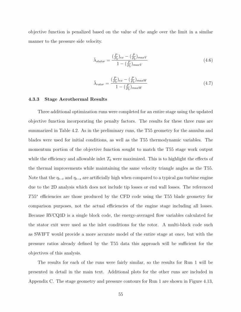
objective function is penalized based on the value of the angle over the limit in a similar
manner to the pressure side velocity.
λstator =( PP0
)ex − ( PP0
)maxV
1− ( PP0
)maxV(4.6)
λrotor =( PP0
)ex − ( PP0
)maxW
1− ( PP0
)maxW(4.7)
4.3.3 Stage Aerothermal Results
Three additional optimization runs were completed for an entire stage using the updated
objective function incorporating the penalty factors. The results for these three runs are
summarized in Table 4.2. As in the preliminary runs, the T55 geometry for the annulus and
blades were used for initial conditions, as well as the T55 thermodynamic variables. The
momentum portion of the objective function sought to match the T55 stage work output
while the efficiency and allowable inlet T0 were maximized. This is to highlight the effects of
the thermal improvements while maintaining the same velocity triangle angles as the T55.
Note that the ηt−t and ηt−s are artificially high when compared to a typical gas turbine engine
due to the 2D analysis which does not include tip losses or end wall losses. The referenced
T55∗ efficiencies are those produced by the CFD code using the T55 blade geometry for
comparison purposes, not the actual efficiencies of the engine stage including all losses.
Because RVCQ3D is a single block code, the energy-averaged flow variables calculated for
the stator exit were used as the inlet conditions for the rotor. A multi-block code such
as SWIFT would provide a more accurate model of the entire stage at once, but with the
pressure ratios already defined by the T55 data this approach will be sufficient for the
objectives of this analysis.
The results for each of the runs were fairly similar, so the results for Run 1 will be
presented in detail in the main text. Additional plots for the other runs are included in
Appendix C. The stage geometry and pressure contours for Run 1 are shown in Figure 4.13,
55
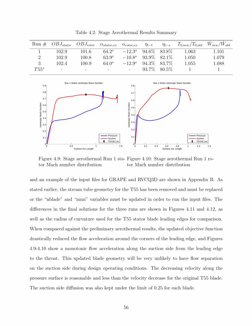
Table 4.2: Stage Aerothermal Results Summary
Run # OBJstator OBJrotor αstator,ex αrotor,ex ηt−t ηt−s T0,new/T0,old Wnew/Wold
1 102.9 101.6 64.2o −12.3o 94.6% 83.8% 1.063 1.1012 102.9 100.8 63.9o −10.8o 93.9% 82.1% 1.050 1.0793 102.4 100.9 64.0o −12.9o 94.3% 83.7% 1.055 1.088
T55∗ - - - - 93.7% 80.5% 1 1
0 0.5 1 1.50
0.1
0.2
0.3
0.4
0.5
0.6
0.7
0.8
0.9Run 1 Stator Isentropic Mach Number
Surface Arc Length
Isen
trop
ic M
ach
Num
ber
PressureSuctionThroat Loc
Figure 4.9: Stage aerothermal Run 1 sta-tor Mach number distribution
0 0.2 0.4 0.6 0.8 1 1.2 1.40
0.1
0.2
0.3
0.4
0.5
0.6
0.7
0.8Run 1 Rotor Isentropic Mach Number
Surface Arc Length
Isen
trop
ic M
ach
Num
ber
PressureSuctionThroat Loc
Figure 4.10: Stage aerothermal Run 1 ro-tor Mach number distribution
and an example of the input files for GRAPE and RVCQ3D are shown in Appendix B. As
stated earlier, the stream tube geometry for the T55 has been removed and must be replaced
or the “nblade” and “nmn” variables must be updated in order to run the input files. The
differences in the final solutions for the three runs are shown in Figures 4.11 and 4.12, as
well as the radius of curvature used for the T55 stator blade leading edges for comparison.
When compared against the preliminary aerothermal results, the updated objective function
drastically reduced the flow acceleration around the corners of the leading edge, and Figures
4.9-4.10 show a monotonic flow acceleration along the suction side from the leading edge
to the throat. This updated blade geometry will be very unlikely to have flow separation
on the suction side during design operating conditions. The decreasing velocity along the
pressure surface is reasonable and less than the velocity decrease for the original T55 blade.
The suction side diffusion was also kept under the limit of 0.25 for each blade.
56
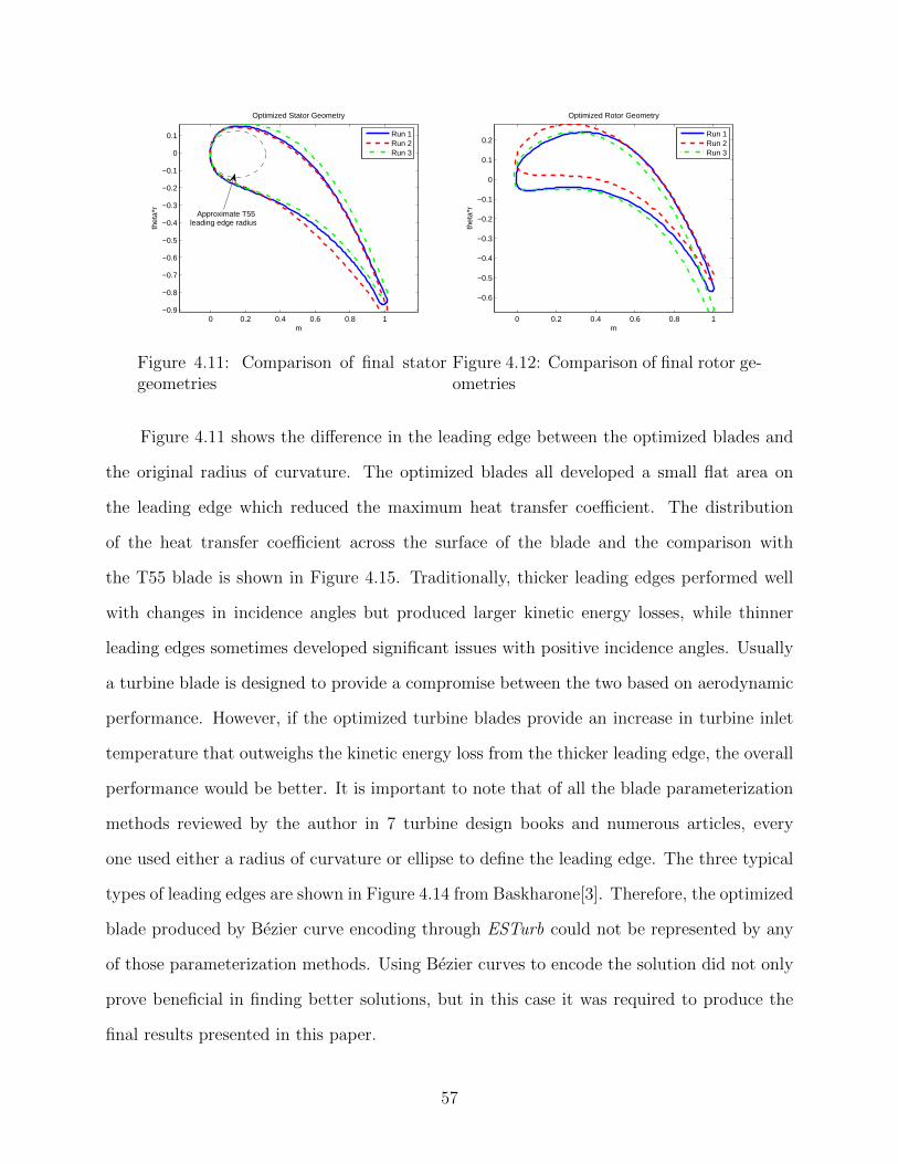
0 0.2 0.4 0.6 0.8 1−0.9
−0.8
−0.7
−0.6
−0.5
−0.4
−0.3
−0.2
−0.1
0
0.1
Optimized Stator Geometry
m
thet
a*r
Run 1Run 2Run 3
Approximate T55 leading edge radius
Figure 4.11: Comparison of final statorgeometries
0 0.2 0.4 0.6 0.8 1
−0.6
−0.5
−0.4
−0.3
−0.2
−0.1
0
0.1
0.2
Optimized Rotor Geometry
m
thet
a*r
Run 1Run 2Run 3
Figure 4.12: Comparison of final rotor ge-ometries
Figure 4.11 shows the difference in the leading edge between the optimized blades and
the original radius of curvature. The optimized blades all developed a small flat area on
the leading edge which reduced the maximum heat transfer coefficient. The distribution
of the heat transfer coefficient across the surface of the blade and the comparison with
the T55 blade is shown in Figure 4.15. Traditionally, thicker leading edges performed well
with changes in incidence angles but produced larger kinetic energy losses, while thinner
leading edges sometimes developed significant issues with positive incidence angles. Usually
a turbine blade is designed to provide a compromise between the two based on aerodynamic
performance. However, if the optimized turbine blades provide an increase in turbine inlet
temperature that outweighs the kinetic energy loss from the thicker leading edge, the overall
performance would be better. It is important to note that of all the blade parameterization
methods reviewed by the author in 7 turbine design books and numerous articles, every
one used either a radius of curvature or ellipse to define the leading edge. The three typical
types of leading edges are shown in Figure 4.14 from Baskharone[3]. Therefore, the optimized
blade produced by Bezier curve encoding through ESTurb could not be represented by any
of those parameterization methods. Using Bezier curves to encode the solution did not only
prove beneficial in finding better solutions, but in this case it was required to produce the
final results presented in this paper.
57
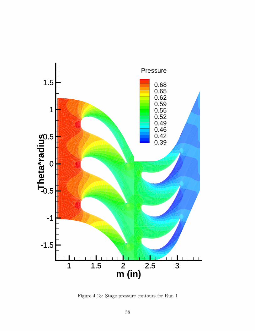
m (in)
Th
eta*
rad
ius
1 1.5 2 2.5 3
-1.5
-1
-0.5
0
0.5
1
1.5
Pressure
0.680.650.620.590.550.520.490.460.420.39
1 1.5 2 2.5 3
-1.5
-1
-0.5
0
0.5
1
1.5
Figure 4.13: Stage pressure contours for Run 1
58
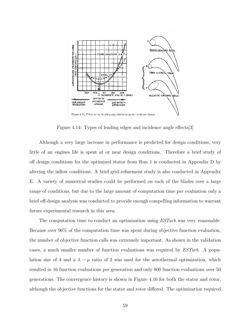
Figure 4.14: Types of leading edges and incidence angle effects[3]
Although a very large increase in performance is predicted for design conditions, very
little of an engines life is spent at or near design conditions. Therefore a brief study of
off design conditions for the optimized stator from Run 1 is conducted in Appendix D by
altering the inflow conditions. A brief grid refinement study is also conducted in Appendix
E. A variety of numerical studies could be performed on each of the blades over a large
range of conditions, but due to the large amount of computation time per evaluation only a
brief off-design analysis was conducted to provide enough compelling information to warrant
future experimental research in this area.
The computation time to conduct an optimization using ESTurb was very reasonable.
Because over 96% of the computation time was spent during objective function evaluation,
the number of objective function calls was extremely important. As shown in the validation
cases, a much smaller number of function evaluations was required by ESTurb. A popu-
lation size of 4 and a λ − µ ratio of 2 was used for the aerothermal optimization, which
resulted in 16 function evaluations per generation and only 800 function evaluations over 50
generations. The convergence history is shown in Figure 4.16 for both the stator and rotor,
although the objective functions for the stator and rotor differed. The optimization required
59

−1 −0.5 0 0.5 1Arc Length Distance from Leading Edge
Hea
t Tra
nsfe
r C
oeffi
cien
t "H
"
Run 1Run 2Run 3T55
Pressure Side Suction Side
Figure 4.15: Heat transfer coefficient for optimized stator
approximately 14 hours to complete on a 2.2 GHz dual core processor and only 5.5 hours to
complete on a 3.4 GHz 8-Core processor per blade row. This resulted in a total of approx-
imately 28 hours or 9 hours of computation time respectively for the entire stage. This is
extremely reasonable given a Navier-Stokes CFD code was used for the function evaluation,
and would allow much higher fidelity codes to be used without making the computation time
excessively high. Parallel processing was not implemented for this analysis, but could easily
be incorporated into the algorithm in the future.
60

0 5 10 15 20 25 30 35 40 45 5060
65
70
75
80
85
90
95
100
105
Generation
Obj
ectiv
e F
unct
ion
Val
ue
Stator Run 1Stator Run 2Rotor Run 1Rotor Run 2Stator Run 3Rotor Run 3
Figure 4.16: Convergence history for both stator and rotor
61
Chapter 5
Conclusions and Future Applications
The three objectives for this thesis were to produce and validate an optimizer, conduct
a turbine aerodynamic optimization, and conduct a turbine aerothermal optimization. The
ESTurb optimizer produced performed remarkably well during the validation cases on airfoil
geometries. The ES optimization algorithm coupled with Bezier curve solution encoding was
well suited for aerodynamic problems and performed a very efficient and effective search to
produce optimal or near optimal solutions. The inviscid turbine aerodynamic optimization
successfully created an objective function to evaluate turbine blade geometry, and validated
the use of Bezier curves in representing turbine blades. The viscous analysis showed the
potential of finding optimal turbine blades that increased efficiency by over 1% and increased
shaft power by 7% over the original T55 blade geometry.
The aerothermal analysis provided the most compelling results of the paper, showing
that using Bezier curves to represent the blade geometry may produce turbine blades that
have better heat transfer characteristics at the leading edge. This improved geometry may
allow up to a 6% increase in turbine inlet temperature, which would correlate to over a 10%
increase in power for an ideal engine. The algorithm also performed an efficient search that
only required 512
hours to complete on a 3.4 GHz desktop computer. Based on these findings,
the following major conclusions may be made:
1. Using an Evolution Strategies algorithm coupled with a Bezier curve encoding is a very
efficient and effective technique for aerodynamic optimization
2. The reduced number of function calls required for an ES algorithm may allow higher
fidelity evaluation methods, such as 3D Navier-Stokes CFD codes, to be used for opti-
mization without unreasonable computation times.
62
3. The aerothermal optimization results show compelling evidence that further research
is needed in this area. Specifically, conducting experimental research to evaluate if the
optimized blades produced in this paper show improved performance over the existing
turbine blades.
Future work in this area should include application of ESTurb or similar algorithms
to other problems in order to determine effectiveness and flexibility across a wide range of
aerospace or other engineering disciplines. Continued research using ESTurb to optimize
turbine blades with higher fidelity 3D models will be pursued by the author, specifically
using SWIFT for a 3D flow solver. Continued research into the validity of the optimized
aerothermal blades by those experienced in turbine design would greatly benefit this area
of research, especially experimental tests to confirm or deny the predictions made by CFD.
Research into the effects of blade geometry on film cooled turbine blades would also prove
very beneficial.
63
Bibliography
[1] Mattingly, Jack D. Elements of Gas Turbine Propulsion. New York: McGraw-Hill, 1996.Print.
[2] Aungier, Ronald H. Turbine Aerodynamics: Axial-flow and Radial-inflow Turbine De-sign and Analysis. New York: ASME, 2006. Print.
[3] Baskharone, Erian A. Principles of Turbomachinery in Air-breathing Engines. Cam-bridge: Cambridge UP, 2006. Print.
[4] Wilson, David Gordon., and Theodosios Korakianitis. The Design of High-efficiencyTurbomachinery and Gas Turbine. Upper Saddle River, NJ: Prentice Hall, 1998. Print.
[5] Lakshminarayana, B. Fluid Dynamics and Heat Transfer of Turbomachinery. New York:Wiley, 1996. Print.
[6] Arts, T., and M. Lambert De Rouvroit. ”Aero-Thermal Performance of a Two-Dimensional Highly Loaded Transonic Turbine Nozzle Guide Vane: A Test Case forInviscid and Viscous Flow Computations.” Journal of Turbomachinery 114.1 (1992):147. Print.
[7] Horlock, J. H., and J. D. Denton. ”A Review of Some Early Design Practice UsingComputational Fluid Dynamics and a Current Perspective.” Journal of Turbomachinery127.1 (2005): 5. Print.
[8] Denton, J. D., and W. N. Dawes. ”Computational fluid dynamics for turbomachinerydesign.” Proceedings of the Institution of Mechanical Engineers, Part C: Journal ofMechanical Engineering Science 213.2 (1998): 107-124.
[9] Chima, Rodrick V. Analysis of Inviscid and Viscous Flows in Cascades with an ExplicitMultiple-grid Algorithm. Washington, D.C.: National Aeronautics and Space Adminis-tration, 1984. Print.
[10] Chima, Rodrick V. A K-ω Turbulence Model for Quasi-three-dimensional Turbomachin-ery Flows. Washington, D.C.: National Aeronautics and Space Administration, 1995.Print.
[11] Chima, Rodrick V., P. W. Giel, and Robert J. Boyle. An Algebraic Turbulence Modelfor Three-dimensional Viscous Flows. Washington, DC: National Aeronautics and SpaceAdministration, 1993. Print.
64
[12] Chima, Rodrick V. ”Application of the K-omega Turbulence Model to Quasi-three-dimensional Turbomachinary Flows.” Journal of Propulsion and Power 12.6 (1996):1176-179. Print.
[13] Goel, S., Cofer, J.I., & Singh H. (June 10-13 1996). Turbine Airfoil Design Optimization,International Gas Turbine and Aeroengine Congress and Exposition, Birmingham, UK.
[14] Giannakoglou, C.K. “A Design Method for Turbine Blades Using Genetic Algorithmson Parallel Computers”, ECCOMAS 98 John Wiley & Sons, 1998.
[15] Giannakoglou, K. C. ”Designing turbomachinery blades using evolutionary methods.”ASME Paper (1999).
[16] Pierret, Stphane, and R. A. Van den Braembussche. ”Turbomachinery blade designusing a NavierStokes solver and artificial neural network.” Journal of Turbomachinery121.2 (1999): 326-332.
[17] Trigg, M. A., G. R. Tubby, and A. G. Sheard. ”Automatic genetic optimization approachto two-dimensional blade profile design for steam turbines.” Journal of turbomachinery121.1 (1999): 11-17.
[18] Dennis, Brian H., George S. Dulikravich, and Zhen-Xue Han. ”Constrained shape opti-mization of airfoil cascades using a Navier-Stokes solver and a genetic/SQP algorithm.”ASME International Gas Turbine and Aeroengine Congress and Exhibition, Indianapo-lis, IN. Vol. 7. No. 10. 1999.
[19] Chen, Bo, and Xin Yuan. ”Advanced aerodynamic optimization system for turboma-chinery.” Journal of turbomachinery 130.2 (2008): 021005.
[20] ksz, zhan, and Ibrahim Sinan Akmandor. ”Multi-Objective Aerodynamic Optimizationof Axial Turbine Blades Using a Novel Multilevel Genetic Algorithm.” Journal of Tur-bomachinery 132.4 (2010): 041009.
[21] Aungier, Ronald H. Axial-Flow Compressors: A Strategy for Aerodynamic Design andAnalysis. New York: ASME, 2003. Print.
[22] Dreo, Johann. Metaheuristics for Hard Optimization: Methods and Case Studies. Berlin:Springer, 2006. Print.
[23] Giannakoglou, K. C. ”Designing turbomachinery blades using evolutionary methods.”ASME Paper (1999).
[24] Wickramasinghe, U., Carrese, R., Li, X. Designing Airfoils using a Reference Point basedEvolutionary Many-objective Particle Swarm Optimization Algorithm. Paper presentedat the IEEE World Congress on Computational Intelligence, Barcelona Spain, July18-23, 2010.
[25] DAngelo, S., Minisci, E. Multi-objective evolutionary optimization of subsonic airfoilsby meta-modeling and evolution control. Proceedings of the Institution of MechanicalEngineers, Part G: Journal of Aerospace Engineering Vol. 221, 2007, pp. 805-814.
65
[26] Curriston, Drew A., and Alice E. Smith. ”Airfoil Optimization by Evolution Strategies.”Evolutionary Computation (CEC), 2013 IEEE Congress on. IEEE, 2013.
[27] Curriston, Drew A., and Roy J. Hartfield. ”Power Turbine Blade Aerodynamic Op-timization Using Non-Restrictive Evolution Strategies.” Joint Propulsion Conference,2013.
[28] Thompson, Joe F., B. K. Soni, and N. P. Weatherill. Handbook of Grid Generation.Boca Raton, FL: CRC, 1999. Print.
[29] Liou, Meng-Sing. ”A Sequel to AUSM: AUSM+.” Journal of computational Physics129.2 (1996): 364-382.
[30] Chima, Rodrick V. ”RVCQ3D Rotor Viscous Code Quasi-3-D User’s Manual and Doc-umentation.” (1999).
[31] Boyle, R. J. ”NavierStokes Analysis of Turbine Blade Heat Transfer.” Journal of Tur-bomachinery 113.3 (1991): 392. Print.
[32] Chima, Rodrick V. Calculation of multistage turbomachinery using steady characteris-tic boundary conditions. Vol. 206613. National Aeronautics and Space AdministrationLangley Research Center, 1998.
[33] Boyce, Meherwan P., Gas Turbine Engineering Handbook. Houston: Gulf PublishingCo., 1982.
[34] Cohen, Henry., Rogers, G.F.C., Saravanamuttoo, H.I.H. Gas Turbine Theory 3rd edi-tion. New York: Wiley & Sons, 1987.
[35] Fielding, L. Turbine Design, The Effect on Axial Turbine Performance of ParameterVariation. New York: ASME Press, 2000.
[36] Pritchard, L. J. An Eleven Parameter Axial Turbine Airfoil Geometry Model. ASMEPaper No. 85-GT-219.
[37] Ye, Z.-Q. A Systematic Computational Design System for Turbine Cascades, AirfoilGeometry and Blade-to-Blade Analysis. Trans. ASME, Journal of Engineering for GasTurbines and Power (July 1984): 598-605.
66

Appendices
67

Appendix A
Pseudo Code for ESTurb
Randomly select or seed initial population of size µ
Evaluate fitness of initial population
Perform generation loop until stopping criteria is met {
for i = 1 to µ {
randomly select parent based on uniform probability
mutate to generate λ/µ offspring
evaluate fitness of each offspring
} end for
sort offspring and parents based on fitness
µ best solutions from λ+ µ replace population
implement one fifth rule
} End generation loop
Save and display results
68

Appendix B
Example GRAPE and RVCQ3D input files
Example GRAPE input file
&grid1 jmax=169 kmax=45 ntetyp=3 nairf=5 nibdst=7 nobshp=7 jairf=229 jtebot=41 jtetop=129 norda=0 3 maxita=0 300
nout=4 xle=2.335500 xte=3.058800 xleft=1.973850 xright=3.420450 rcorn=0 dsi=1.000e-05 &end
&grid2 nobcas=0 nle=35 nte=24 dsra=0.500000 dsle=0.006000 dste=0.001000 pitch=0.608508 yscl=1.000000 xtfrac=1.000000
dsobi=0.013522 aaai=0.550000 bbbi=0.550000 ccci=0.700000 dddi=0.700000 csmoo=0 jcap=18 dswex=0.008000 jwakex=1 kwakex=1
joble=9 fswake=0.600000 &end
&grid3 airfx=
7.20223359E-01 7.19743354E-01 7.19250123E-01 7.18748279E-01 7.18242519E-01 7.17737573E-01 7.17238166E-01 7.16748968E-01
7.16274558E-01 7.15819372E-01 7.15387670E-01 7.14983490E-01 7.14610614E-01 7.14272529E-01 7.13972398E-01 7.13713029E-01
7.11596086E-01 7.09150004E-01 7.06377036E-01 7.03279756E-01 6.99861057E-01 6.96124144E-01 6.92072523E-01 6.87710001E-01
6.83040675E-01 6.78068925E-01 6.72799408E-01 6.67237054E-01 6.61387053E-01 6.55254857E-01 6.48846164E-01 6.42166917E-01
6.35223298E-01 6.28021715E-01 6.20568804E-01 6.12871414E-01 6.04936605E-01 5.96771641E-01 5.88383982E-01 5.79781278E-01
5.70971361E-01 5.61962241E-01 5.52762094E-01 5.43379263E-01 5.33822245E-01 5.24099685E-01 5.14220373E-01 5.04193234E-01
4.94027321E-01 4.83731811E-01 4.73315994E-01 4.62789272E-01 4.52161147E-01 4.41441217E-01 4.30639169E-01 4.19764771E-01
4.08827866E-01 3.97838368E-01 3.86806249E-01 3.75741539E-01 3.64654313E-01 3.53554691E-01 3.42452826E-01 3.31358897E-01
3.20283109E-01 3.09235677E-01 2.98226826E-01 2.87266781E-01 2.76365762E-01 2.65533977E-01 2.54781614E-01 2.44118835E-01
2.33555770E-01 2.23102509E-01 2.12769095E-01 2.02565520E-01 1.92501716E-01 1.82587547E-01 1.72832806E-01 1.63247205E-01
1.53840369E-01 1.44621832E-01 1.35601024E-01 1.26787272E-01 1.18189787E-01 1.09817662E-01 1.01679860E-01 9.37852135E-02
8.61424117E-02 7.87599983E-02 7.16463624E-02 6.48097326E-02 5.82581699E-02 5.19995613E-02 4.60416127E-02 4.03918425E-02
3.50575746E-02 3.00459318E-02 2.53638289E-02 2.10179664E-02 1.70148231E-02 1.33606499E-02 1.00614629E-02 7.12303646E-03
4.55089684E-03 2.35031512E-03 5.26300639E-04 -9.16405794E-04 -1.97333863E-03 -2.64031430E-03 -2.91343801E-03 -2.78911040E-03
-2.26403437E-03 -1.33522172E-03 0.00000000E+00 1.37412562E-03 3.57375250E-03 6.54814423E-03 1.02483270E-02 1.46270603E-02
1.96388076E-02 2.52397073E-02 3.13875429E-02 3.80417145E-02 4.51632088E-02 5.27145702E-02 6.06598716E-02 6.89646847E-02
7.75960512E-02 8.65224532E-02 9.57137840E-02 1.05141319E-01 1.14777686E-01 1.24596836E-01 1.34574015E-01 1.44685733E-01
1.54909736E-01 1.65224975E-01 1.75611580E-01 1.86050828E-01 1.96525113E-01 2.07017920E-01 2.17513793E-01 2.27998307E-01
2.38458037E-01 2.48880532E-01 2.59254282E-01 2.69568692E-01 2.79814049E-01 2.89981498E-01 3.00063006E-01 3.10051339E-01
3.19940030E-01 3.29723348E-01 3.39396272E-01 3.48954460E-01 3.58394218E-01 3.67712477E-01 3.76906754E-01 3.85975132E-01
3.94916225E-01 4.03729152E-01 4.12413505E-01 4.20969321E-01 4.29397052E-01 4.37697540E-01 4.45871979E-01 4.53921894E-01
4.61849109E-01 4.69655715E-01 4.77344045E-01 4.84916641E-01 4.92376228E-01 4.99725682E-01 5.06968004E-01 5.14106285E-01
5.21143683E-01 5.28083391E-01 5.34928606E-01 5.41682504E-01 5.48348206E-01 5.54928752E-01 5.61427070E-01 5.67845948E-01
5.74188003E-01 5.80455655E-01 5.86651094E-01 5.92776251E-01 5.98832772E-01 6.04821987E-01 6.10744877E-01 6.16602053E-01
6.22393719E-01 6.28119644E-01 6.33779138E-01 6.39371016E-01 6.44893574E-01 6.50344555E-01 6.55721125E-01 6.61019838E-01
6.66236611E-01 6.71366694E-01 6.76404639E-01 6.81344271E-01 6.86178662E-01 6.90900097E-01 6.95500047E-01 6.99969141E-01
7.04297134E-01 7.08472880E-01 7.12484301E-01 7.16318360E-01 7.19961027E-01 7.23397257E-01 7.23499088E-01 7.23552557E-01
7.23557164E-01 7.23512865E-01 7.23420076E-01 7.23279664E-01 7.23092943E-01 7.22861660E-01 7.22587978E-01 7.22274458E-01
7.21924032E-01 7.21539980E-01 7.21125893E-01 7.20685647E-01 7.20223359E-01
airfy=
-4.05503505E-01 -4.05663650E-01 -4.05776673E-01 -4.05841518E-01 -4.05857576E-01 -4.05824698E-01 -4.05743191E-01 -4.05613819E-01
-4.05437790E-01 -4.05216753E-01 -4.04952775E-01 -4.04648325E-01 -4.04306251E-01 -4.03929754E-01 -4.03522357E-01 -4.03087869E-01
-3.99086672E-01 -3.94436305E-01 -3.89183038E-01 -3.83371881E-01 -3.77046599E-01 -3.70249713E-01 -3.63022513E-01 -3.55405064E-01
-3.47436215E-01 -3.39153605E-01 -3.30593676E-01 -3.21791674E-01 -3.12781666E-01 -3.03596539E-01 -2.94268016E-01 -2.84826659E-01
-2.75301878E-01 -2.65721943E-01 -2.56113986E-01 -2.46504015E-01 -2.36916916E-01 -2.27376470E-01 -2.17905350E-01 -2.08525139E-01
69
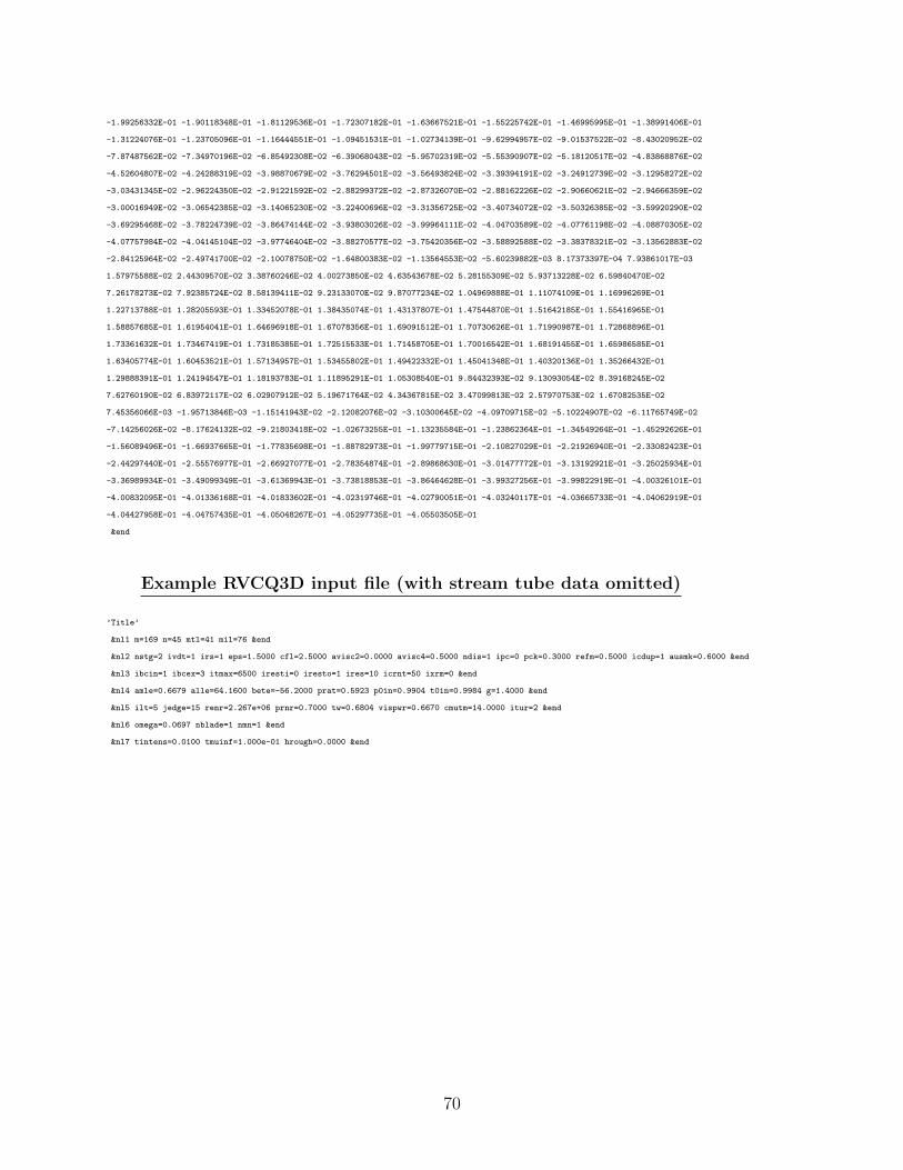
-1.99256332E-01 -1.90118348E-01 -1.81129536E-01 -1.72307182E-01 -1.63667521E-01 -1.55225742E-01 -1.46995995E-01 -1.38991406E-01
-1.31224076E-01 -1.23705096E-01 -1.16444551E-01 -1.09451531E-01 -1.02734139E-01 -9.62994957E-02 -9.01537522E-02 -8.43020952E-02
-7.87487562E-02 -7.34970196E-02 -6.85492308E-02 -6.39068043E-02 -5.95702319E-02 -5.55390907E-02 -5.18120517E-02 -4.83868876E-02
-4.52604807E-02 -4.24288319E-02 -3.98870679E-02 -3.76294501E-02 -3.56493824E-02 -3.39394191E-02 -3.24912739E-02 -3.12958272E-02
-3.03431345E-02 -2.96224350E-02 -2.91221592E-02 -2.88299372E-02 -2.87326070E-02 -2.88162226E-02 -2.90660621E-02 -2.94666359E-02
-3.00016949E-02 -3.06542385E-02 -3.14065230E-02 -3.22400696E-02 -3.31356725E-02 -3.40734072E-02 -3.50326385E-02 -3.59920290E-02
-3.69295468E-02 -3.78224739E-02 -3.86474144E-02 -3.93803026E-02 -3.99964111E-02 -4.04703589E-02 -4.07761198E-02 -4.08870305E-02
-4.07757984E-02 -4.04145104E-02 -3.97746404E-02 -3.88270577E-02 -3.75420356E-02 -3.58892588E-02 -3.38378321E-02 -3.13562883E-02
-2.84125964E-02 -2.49741700E-02 -2.10078750E-02 -1.64800383E-02 -1.13564553E-02 -5.60239882E-03 8.17373397E-04 7.93861017E-03
1.57975588E-02 2.44309570E-02 3.38760246E-02 4.00273850E-02 4.63543678E-02 5.28155309E-02 5.93713228E-02 6.59840470E-02
7.26178273E-02 7.92385724E-02 8.58139411E-02 9.23133070E-02 9.87077234E-02 1.04969888E-01 1.11074109E-01 1.16996269E-01
1.22713788E-01 1.28205593E-01 1.33452078E-01 1.38435074E-01 1.43137807E-01 1.47544870E-01 1.51642185E-01 1.55416965E-01
1.58857685E-01 1.61954041E-01 1.64696918E-01 1.67078356E-01 1.69091512E-01 1.70730626E-01 1.71990987E-01 1.72868896E-01
1.73361632E-01 1.73467419E-01 1.73185385E-01 1.72515533E-01 1.71458705E-01 1.70016542E-01 1.68191455E-01 1.65986585E-01
1.63405774E-01 1.60453521E-01 1.57134957E-01 1.53455802E-01 1.49422332E-01 1.45041348E-01 1.40320136E-01 1.35266432E-01
1.29888391E-01 1.24194547E-01 1.18193783E-01 1.11895291E-01 1.05308540E-01 9.84432393E-02 9.13093054E-02 8.39168245E-02
7.62760190E-02 6.83972117E-02 6.02907912E-02 5.19671764E-02 4.34367815E-02 3.47099813E-02 2.57970753E-02 1.67082535E-02
7.45356066E-03 -1.95713846E-03 -1.15141943E-02 -2.12082076E-02 -3.10300645E-02 -4.09709715E-02 -5.10224907E-02 -6.11765749E-02
-7.14256026E-02 -8.17624132E-02 -9.21803418E-02 -1.02673255E-01 -1.13235584E-01 -1.23862364E-01 -1.34549264E-01 -1.45292626E-01
-1.56089496E-01 -1.66937665E-01 -1.77835698E-01 -1.88782973E-01 -1.99779715E-01 -2.10827029E-01 -2.21926940E-01 -2.33082423E-01
-2.44297440E-01 -2.55576977E-01 -2.66927077E-01 -2.78354874E-01 -2.89868630E-01 -3.01477772E-01 -3.13192921E-01 -3.25025934E-01
-3.36989934E-01 -3.49099349E-01 -3.61369943E-01 -3.73818853E-01 -3.86464628E-01 -3.99327256E-01 -3.99822919E-01 -4.00326101E-01
-4.00832095E-01 -4.01336168E-01 -4.01833602E-01 -4.02319746E-01 -4.02790051E-01 -4.03240117E-01 -4.03665733E-01 -4.04062919E-01
-4.04427958E-01 -4.04757435E-01 -4.05048267E-01 -4.05297735E-01 -4.05503505E-01
&end
Example RVCQ3D input file (with stream tube data omitted)
’Title’
&nl1 m=169 n=45 mtl=41 mil=76 &end
&nl2 nstg=2 ivdt=1 irs=1 eps=1.5000 cfl=2.5000 avisc2=0.0000 avisc4=0.5000 ndis=1 ipc=0 pck=0.3000 refm=0.5000 icdup=1 ausmk=0.6000 &end
&nl3 ibcin=1 ibcex=3 itmax=6500 iresti=0 iresto=1 ires=10 icrnt=50 ixrm=0 &end
&nl4 amle=0.6679 alle=64.1600 bete=-56.2000 prat=0.5923 p0in=0.9904 t0in=0.9984 g=1.4000 &end
&nl5 ilt=5 jedge=15 renr=2.267e+06 prnr=0.7000 tw=0.6804 vispwr=0.6670 cmutm=14.0000 itur=2 &end
&nl6 omega=0.0697 nblade=1 nmn=1 &end
&nl7 tintens=0.0100 tmuinf=1.000e-01 hrough=0.0000 &end
70

Appendix C
Additional Plots for Optimization Runs
71

m (in)
Th
eta*
rad
ius
1 1.5 2 2.5 3
-1.5
-1
-0.5
0
0.5
1
1.5
Pressure
0.680.650.620.590.550.520.490.460.420.39
1 1.5 2 2.5 3
-1.5
-1
-0.5
0
0.5
1
1.5
Figure C.1: Pressure contours for Run 2 stage results
0 0.5 1 1.50
0.1
0.2
0.3
0.4
0.5
0.6
0.7
0.8
0.9
Surface Arc Length
Isen
trop
ic M
ach
Num
ber
PressureSuctionThroat Loc
Figure C.2: Isentropic Mach number dis-tribution for Run 2 stator
0 0.2 0.4 0.6 0.8 1
0.1
0.2
0.3
0.4
0.5
0.6
0.7
0.8
Surface Arc Length
Isen
trop
ic M
ach
Num
ber
PressureSuctionThroat Loc
Figure C.3: Isentropic Mach number dis-tribution for Run 2 rotor
72

m (in)
Th
eta*
rad
ius
1 1.5 2 2.5 3
-1.5
-1
-0.5
0
0.5
1
1.5
Pressure
0.680.650.620.590.550.520.490.460.420.39
1 1.5 2 2.5 3
-1.5
-
Figure C.4: Pressure contours for Run 3 stage results
0 0.5 1 1.50
0.1
0.2
0.3
0.4
0.5
0.6
0.7
0.8
0.9
Surface Arc Length
Isen
trop
ic M
ach
Num
ber
PressureSuctionThroat Loc
Figure C.5: Isentropic Mach number dis-tribution for Run 3 stator
0 0.2 0.4 0.6 0.8 10
0.1
0.2
0.3
0.4
0.5
0.6
0.7
Surface Arc Length
Isen
trop
ic M
ach
Num
ber
PressureSuctionThroat Loc
Figure C.6: Isentropic Mach number dis-tribution for Run 3 rotor
73

Appendix D
Off-Design Effects on Aerothermal Blade
A very brief off-design analysis was conducted on the optimized stator for Run 1. The
Mach number distribution along the blade while varying the incidence angle from −15o to
+15o is shown in Figure D.1. These results show the blade performs well at negative incidence
angles and has a monotonic velocity increase on the suction side up to almost +10o. This
performance is comparable to that of the T55 and most turbine blades, which generally have
a drastic reduction in performance at incidence angles over +10o. A close-up of the suction
surface is shown in Figure D.2
74

0 0.5 1 1.50
0.1
0.2
0.3
0.4
0.5
0.6
0.7
0.8
0.9Isentropic Mach Number for Varying Incidence Angles
Surface Arc Length
Isen
trop
ic M
ach
Num
ber
−15 deg−10 deg−5 deg0 deg5 deg10 deg15 degThroat Loc
Figure D.1: Mach number surface distribution over a range of incidence angles
0.15 0.2 0.25 0.3 0.35
0.64
0.66
0.68
0.7
0.72
0.74
0.76
Isentropic Mach Number for Varying Incidence Angles
Surface Arc Length
Isen
trop
ic M
ach
Num
ber
−15 deg−10 deg−5 deg0 deg5 deg10 deg15 degThroat Loc
Figure D.2: Close-up of Figure D.1 suction side
75
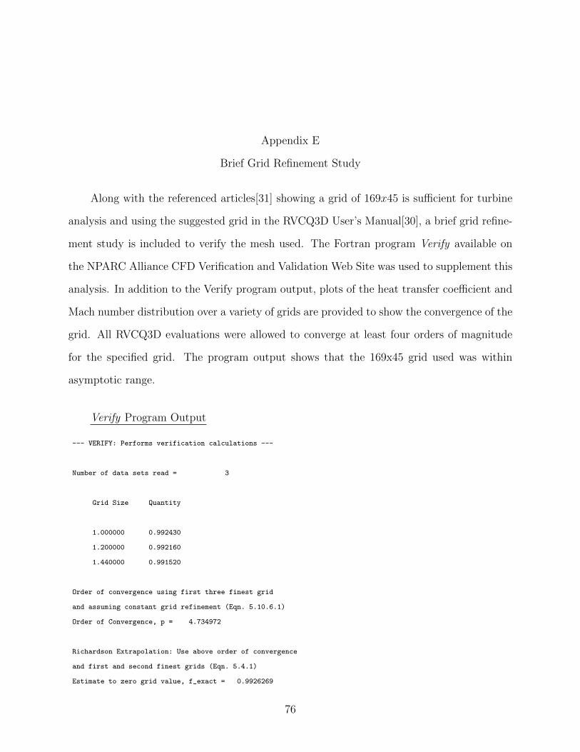
Appendix E
Brief Grid Refinement Study
Along with the referenced articles[31] showing a grid of 169x45 is sufficient for turbine
analysis and using the suggested grid in the RVCQ3D User’s Manual[30], a brief grid refine-
ment study is included to verify the mesh used. The Fortran program Verify available on
the NPARC Alliance CFD Verification and Validation Web Site was used to supplement this
analysis. In addition to the Verify program output, plots of the heat transfer coefficient and
Mach number distribution over a variety of grids are provided to show the convergence of the
grid. All RVCQ3D evaluations were allowed to converge at least four orders of magnitude
for the specified grid. The program output shows that the 169x45 grid used was within
asymptotic range.
Verify Program Output
--- VERIFY: Performs verification calculations ---
Number of data sets read = 3
Grid Size Quantity
1.000000 0.992430
1.200000 0.992160
1.440000 0.991520
Order of convergence using first three finest grid
and assuming constant grid refinement (Eqn. 5.10.6.1)
Order of Convergence, p = 4.734972
Richardson Extrapolation: Use above order of convergence
and first and second finest grids (Eqn. 5.4.1)
Estimate to zero grid value, f_exact = 0.9926269
76

Grid Convergence Index on fine grids. Uses p from above.
Factor of Safety = 1.250000
Grid Refinement
Step Ratio, r GCI(%)
1 2 1.200000 0.024801
2 3 1.200000 0.058818
Checking for asymptotic range using Eqn. 5.10.5.2. A ratio of 1.0 indicates asymptotic range.
Grid Range Ratio
12 23 0.999728
--- End of VERIFY ---
0 1000 2000 3000 4000 5000 6000 700010
−9
10−8
10−7
10−6
10−5
10−4
Iterations
RR
MS
Figure E.1: RRMS plot for 169x45 grid
77

0 0.5 1 1.50
0.1
0.2
0.3
0.4
0.5
0.6
0.7
0.8
Surface Arc Length
Isen
trop
ic M
ach
Num
ber
169x45250x50383x70
Figure E.2: Mach number distribution for multiple grid sizes
−1 −0.5 0 0.5 1Arc Length Distance from Leading Edge
Hea
t Tra
nsfe
r C
oeffi
cien
t "H
" (B
TU
/lbm
.hr.
ft2 )
85x23, dsi=1e−4169x45, dsi=1e−5250x50, dsi=1e−5360x68, dsi=1e−5383x70, dsi=5e−6
Pressure Side Suction Side
Figure E.3: Heat transfer coefficient distribution for multiple grid sizes
78