Aerodynamic Ground Effect: a case-study of the integration of CFD and experiments

Tracie Barber1, Stephen Hall2 1 University of NSW, Sydney, NSW 2052, Australia. t.barber@unsw.edu.au 2 University of NSW, Sydney, NSW 2052, Australia. sd.hall@unsw.edu.au

Keywords: CFD, aerodynamics, ground effect

Abstract: There are still many aspects of ground effect that need clarification. This paper will review the various methods available in the area of ground effect aerodynamic prediction, both computationally and experimentally, and determine their appropriateness. Assumptions are examined, and the use of correct boundary conditions in both experimental and computational procedures is emphasized, as are the importance of the inclusion of viscosity effects in a computational model. It is concluded that for the field of ground effect flight, a combination of CFD and experiments is required to fully understand the resulting flow. Specific examples of ground effect flight that make full use of the integration of CFD and experiments will be given, including the design and construction of a moving ground facility for the UNSW subsonic 3ft x 4ft wind tunnel.

Introduction The concept of using ground effect as an aerodynamic advantage has long been recognised. Industries internationally are designing Wing-In-Ground (WIG) vehicles, which combine the concepts of naval architecture and aerospace engineering to produce vehicles that fly just metres above the water surface(1,2,3). Naval architects are also considering the benefits of ground effect in the design of high speed craft, to use the aerodynamic lift generated, to reduce the hydrodynamic drag, by lifting the vehicle out of the water(4). Automotive industries, particularly those involved in high-speed, use ground effect forces to increase downforce and increase possible cornering speeds(5). However, much of the research in the area of ground effect aerodynamic prediction is either unreliable or inconclusive. Assumptions used often exclude the exact conditions of interest to the designer. Experimental results are scarce and these too are frequently unreliable. Regarding Wing-In-Ground effect vehicles, Steinbach and Jacob(6) observed, “it seems that basic aerodynamic … considerations were often left in the background or were even disregarded. A positive ground effect for the vehicles, that is a higher lift and better lift to drag ratio near ground, was mostly assumed in advance.” Frequently, discrepancies between the published results are found. Walker et al(7) noted that “recent theoretical and experimental studies [in the area of ground effect] … often report significant differences between computational and experimental results”. These discrepancies are generally due to an incorrect specification of the ground surface boundary conditions, or an inappropriate use of an otherwise correct model. For example, some analytical solutions (see for example Rozhdestvensky(8)) are accurate for certain clearances only; these type of restrictions are sometimes not observed when the results are used by other researchers. Traditional procedures that do not take into account the viscous effects are commonly used for the design of these vehicles, and this can cause over-prediction in efficiency values, due to the drag forces being under-predicted. Chun and Park(9) noted that the panel method (an inviscid numerical method) “appears to have limits in predicting forces near the ground” and Katz(10) suggested that “in real flow situations, the increase in lift will be limited by viscous effects”. While experimental or computational simulation can be a convenient alternative to full-scale testing, the incorporation of the surface effects often leads to confusion due to such a model being in a vehicle fixed reference frame (air moving, vehicle fixed) rather than the real-life situation of a ground fixed reference frame (air fixed, vehicle moving). Various forms of boundary condition have been specified for the ground and some in common use result in incorrect solutions. A definitive outline of the requirements for modeling ground effect is required. Three main areas of ambiguity are apparent:

• Of the various boundary conditions suggested (both computational and experimental) which are appropriate?

• Specifically for vehicles operating over water, is a rigid ground a reasonable assumption?

1

• Are methods based on potential flow accurate enough for ground effect analyses, or is a viscous solution required?

Computational Fluid Dynamics (CFD) results and Particle Image Velocimetry (PIV) results are presented. It is found that only through an integrated study, making use of the advantages of both experiments and CFD, can a good understanding of ground effect be found. The requirement that a correct, realistic boundary condition be used means that in certain cases, a CFD simulation is the only feasible option.

Methods of specifying the Ground Boundary Condition As will be detailed later in the paper, the University of New South Wales is currently updating the experimental facilities for ground effect simulation. The strong interest in ground effect studies, along with an understanding of the requirements for accurate simulation (both for experimental testing and CFD simulation), has led to this upgrade. Some of the background research that has led to this understanding is discussed. The apparent uncertainty as to the correct boundary condition to use for the ground is demonstrated by the 1995 paper by Hsiun and Chen(11), on the study of the aerodynamic characteristics of an airfoil in ground effect. The flow was assumed to be laminar, incompressible and viscous. The boundary condition used on the ground was reported as “the no-slip condition, so u=0, v=0”. (This condition is the equivalent of a wind tunnel test with a stationary ground). Six airfoil shapes were considered, and the authors concluded that the lift and drag characteristics are dependent on the channel formed by the lower surface of the airfoil and the ground. In a note referring to the paper of Hsiun and Chen, Steinbach(12) explained that the “correct boundary condition is slip (u=1, v=0)”, with u and v being variables non-dimensionalised to the freestream. However, this is an uncertain explanation, as the slip condition has varying meanings among aerodynamicists and CFD practitioners; in CFD terminology it is taken to mean a condition of zero shear stress at the boundary. This suggestion of “slip” conflicts with the latter part of Steinbach’s explanation, as the condition of “(u=1, v=0)” is clearly a condition of the ground moving at the freestream velocity. Later in the paper, the author suggests that a “reflected grid” (a symmetry boundary condition) is recommended, this being the third “correct” condition. Of four possible (common) boundary conditions, the first, defined here as “Image”, refers to the use of the image method, first suggested by Wieselsberger(13). Setting the lower boundary to be a symmetry condition (in CFD) is also the use of the “Image” condition. The second condition, defined here as “Slip”, refers to the condition in which there is zero shear stress at the boundary. It can be seen that this type of condition could allow the ground to be moving at different velocities depending on its position relative to the vehicle, to enforce the zero shear stress condition. The difference between these two conditions is that for a symmetry boundary all normal gradients are set to zero, and for a slip wall only the normal component of velocity is set to zero. In certain cases, this can cause a difference in the final solution between these conditions. The third condition, defined here as “Ground Stationary”, refers to the type of condition set by Hsiun and Chen. However, by considering the actual flow situation, it can be seen that this condition is not appropriate. In a ground-fixed reference frame, the air is stationary, the ground is stationary, and the body flies over the ground and through the air at velocity, U∞. By moving to a vehicle-fixed reference frame it can be seen that the vehicle is stationary, and both the freestream air and ground should be moving relative to the body at the freestream velocity, U∞. Setting the ground to be moving at U∞, is the final (and physically correct) condition, defined here as “Ground Moving”. The ground is given the same velocity as that of the freestream, a condition accurately representing that of the real-life situation. George(14) conducted an experimental investigation of bluff bodies, and recommended that for ground clearances of less than 10% of the model height, the moving ground plane simulation must be used. Diuzet(15) showed some differences in the flow field around a cylinder near the ground, when comparing the image, moving ground and stationary ground simulations. The effect of the ground simulation was also the subject of an informative study by Fago et al(16), who concluded that the “only accurate simulation technique is the moving ground simulation.” The authors compared the various methods available for ground simulation, and remarked that suction and image techniques are generally regarded as being equivalent to the moving belt technique due to the absence of a boundary layer build-up. However, they reasoned that this is an incorrect assumption, as unlike normal operating conditions, the velocity gradient at the boundary disappears. Hucho and Sorvan(17) outlined the various methods available to model the ground in wind tunnel testing (for automotive testing). Suggestions included the use of a solid and fixed floor, two identical models with a plane of symmetry between them (the image method), a slot to remove the boundary layer, holes beneath the vehicle to

2

remove the boundary layer, and a moving belt in combination with a suction slot to remove the oncoming boundary layer. In a study of the aerodynamics of Gurney flaps on wings in ground effect, Zerihan and Zhang(18) used a moving ground wind tunnel, noting that “it is the authors opinion that not only can a freestream study not be applied to the situation in ground effect but also any fixed-ground studies should also be viewed with caution because different fluid flow features may exist.”

CFD Analysis To determine the most appropriate boundary conditions, the NACA 4412 airfoil was studied in various ground effect conditions, using CFD. This airfoil is commonly used for the study of ground effect problems, and the angle of attack was 2.9 degrees, Reynolds number was 8,200,000 and the freestream velocity was 108.7m/s. All boundary conditions are enforced on the same model. Each ground clearance required a different grid, however the main section of the grid remains the same and further sections of similar density grid were added to increase the ground clearance. At the upstream boundary, a uniform onset flow was specified. The upper boundary was set as a pressure boundary, as was the downstream boundary. The lower boundary was set depending on the particular model being investigated. This may be either a wall with a certain velocity or a symmetry condition. A commercial CFD solver, CFX4, has been used to solve for the flow field. The equations solved are the Navier Stokes equations:

( ) 0=⋅∇+∂∂ Ut

ρρ (1)

xzxyxxx SzyxxDt

Du +∂

∂+∂

∂+

∂∂+

∂∂−= τττρρ

(2)

yzyyyxy SzyxyDt

Dv +∂

∂+

∂∂

+∂

∂+

∂∂−=

τττρρ (3)

zzzyzxz SzyxzDt

Dw +∂

∂+∂

∂+

∂∂+

∂∂−= τττρρ

(4)

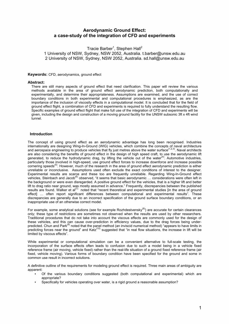
representing continuity and momentum. The RNG k-ε turbulence model was used to close the set of equations and the Van Leer (higher order) scheme was used for discretization. To first validate the numerical computation of the present study, results are calculated for the airfoil in free air, and compared to experimental results(19). The model predicts the Cp curve well, with small differences on the suction side of the airfoil. Grid Convergence Index (GCI) values(20) have been calculated for each of the grids. The error in using the fine grid (used in the investigation) ranges from 1% to 3% for Cl, and is around 11% for Cd. The results for the iterative convergence study showed that the value for the convergence criterion can be set at 1x10-5 and achieve excellent levels of accuracy. Two-dimensional results for the airfoil near the ground were obtained for the four different cases, at varying values of h/c (ratio of height of trailing edge above ground surface to chord). The differing predictions at the smallest clearance of h/c=0.025, for the four models are clearly demonstrated in Figure 1, comparing velocity profiles for each model. A recirculation region in the Ground Stationary model is visible beneath the leading edge of the airfoil, and the similar effect in the Image model can be seen. No recirculation region is visible in either the Slip or Ground Moving models although a trend towards this is seen in the Slip model, where the velocity vectors are slowing at the wall. In comparison, velocity vectors for the Ground Moving model show an increase in velocity as the air speeds up to meet the velocity of the wall.

3

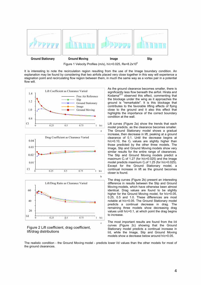
Figure 1 Velocity Profiles (m/s), h/c=0.025, Re=8.2x10 is interesting to note the recirculation region resulting from the use of the Image boundary condition. An

As the ground clearance becomes smaller, there is

ft curves (Figure 2a) show the trends that each

he drag curves (Figure 2b) present an interesting

he most important results are found from the l/d

The realistic condition - the Ground Moving model - predicts lower l/d values than the other models for most of

6

Ground MovingGround Stationary Image Slip

0 35 73 110 147

Ground Stationary Ground Moving Image Slip

Itexplanation may be found by considering that two airfoils placed very close together in this way will experience a stagnation point and recirculating flow region between them, in much the same way as a vortex pair in a potential flow will.

0 0.25 0.5 0.75 1h/c

0.7

0.8

0.9

1

1.1

1.2

1.3

1.4

Cl

Free Air ReferenceSlipGround StationaryImageGround Moving

Lift Coefficient as Clearance Varied

0 0.25 0.5 0.75 1h/c

0

0.01

0.02

0.03

0.04

Cd

Free Air ReferenceSlipGround StationaryImageGround Moving

Drag Coefficient as Clearance Varied

0 0.25 0.5 0.75 1h/c

10

20

30

40

50

60

70

l/d

Free Air ReferenceSlipGround StationaryImageGround Moving

Lift/Drag Ratio as Clearance Varied

a

b

c

Free Air ReferenceSlipGround StationaryImageGround Moving1.0

0.8

1.2

1.4

0 0.25 0.5 0.75 1 h/c

0 0.25 0.5 0.75 1 h/c

0 0.25 0.5 0.75 1 h/c

Cl

0.02

0.01

0.03

0.04

Cl

20

40

60

l/d

Figure 2 Lift coefficient, drag coefficient, lift/drag distributions

significantly less flow beneath the airfoil. Hirata and Kodama(21) observed this effect, commenting that the blockage under the wing as it approaches the ground is "remarkable". It is this blockage that contributes to the favorable lifting effects of flying close to the ground and it also this effect that highlights the importance of the correct boundary condition at the wall. Limodel predicts, as the clearance becomes smaller. The Ground Stationary model shows a gradual increase, then decrease in lift, peaking at a ground clearance of 0.1. Until the decrease begins at h/c=0.10, the Cl values are slightly higher than those predicted by the other three models. The Image, Slip and Ground Moving models show very similar results for the entire range of clearances. The Slip and Ground Moving models predict a maximum Cl of 1.27 (for h/c=0.025) and the Image model predicts maximum Cl of 1.25 (for h/c=0.025). Except for the Ground Stationary model, a continual increase in lift as the ground becomes closer is found. Tdifference in results between the Slip and Ground Moving models, which have otherwise been almost identical. Drag values are found to be slightly higher for the Ground Moving model, for h/c=0.05, 0.25, 0.5 and 1.0. These differences are most notable at h/c=0.05. The Ground Stationary model predicts a continual decrease in drag. The remaining three models show decreasing drag values until h/c=0.1, at which point the drag begins to increase. Tcurves (Figure 2c) showing that the Ground Stationary model predicts a continual increase in l/d, while the Image, Slip and Ground Moving models show a decrease below around h/c=0.05.

the ground clearances.

4

PIV Analysis For further insight into the flowfield near the moving ground, PIV experiments were run and compared with CFD results. PIV is an experimental technique that relies on the measurement of particle displacement within a flow field. The particles are illuminated with a high intensity laser light sheet, and pairs of images are acquired at small time intervals apart, by pulsing the laser and considerating the time intervals and particle displacements allows the instantaneous velocity vectors to be determined. To illuminate the particles in the flow field, a twin-head pulsed Nd-Yag laser was used. The laser system produced an output wavelength of 532nm (green) and output energy of 100 mJ/pulse. For the current investigation, the pulse separation was set at 60µs, and the laser was capable of a double pulse rate of 20Hz. A light delivery system ensured that the circular pulsed laser beam was delivered to the flow field as a plane sheet of light with almost uniform thickness of 2mm. The seeding particles selected for this investigation were spherical latex particles with a mean diameter of 5µm, producing minimal slip. A commercial analysis program, Visiflow, was used for statistical analysis of the flow. (For further details on the design and construction of the system see Hall(22)). The tunnel was constructed of clear acrylic and a 10kW fan generated airspeeds of 15m/s in a rectangular test section. A step was formed at the test section, and this allowed the placement of a conveyor belt system to simulate a moving ground.

Camera

Conveyor Belt

Wing

Drive System Conveyor Belt

Win g

Drive System

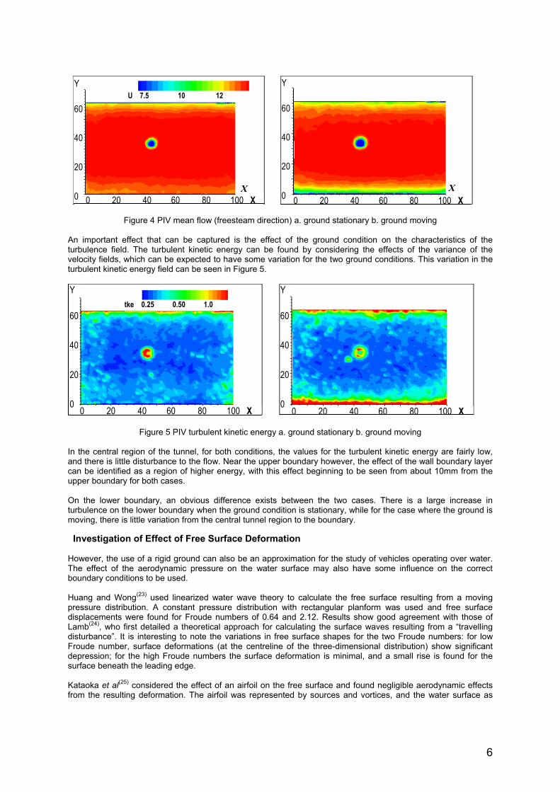
Figure 3 Two Phase Tunnel with Conveyor System A conveyor system frame was designed and constructed from acrylic, with a 2mm thick rubber belt to act as the moving ground. The conveyor system is 600mm long by 202mm belt width, allowing a test section of 202mm x 67mm area above the belt. A drive powered the system with a flexible coupling connecting the drive shaft. This enabled the belt to be driven at speeds matching the wind tunnel airspeed, which for this investigation was 15m/s. An optical tachometer was used to ensure correct belt velocity. A slot ahead of the belt ensured that any oncoming boundary layer was removed and a suction region existing below the slot (due to the lower pressure existing behind the step region) aided in boundary layer removal. Two sets of data were recorded; the first represented a stationary ground situation (conveyor off) and the second represented a moving ground situation (conveyor on). For these initial cases, no lifting surface was present in the test-section. After analysis of the acquired images as outlined above, the mean flow field was obtained. Figure 4 compares the mean flow in the freestream direction for the two cases of the ground moving and the ground stationary. The results are given in the form of flooded contours, as this is the most convenient way to present the amount of information found for the PIV results (the discrepancy in the central region for both of these cases is due to an irregularity in the acrylic wall). For the case with the ground moving, the flow remains nearly uniform as it approaches the lower boundary. A boundary layer exists at the upper boundary, where the wall is stationary. However, with the conveyor turned off, the effect of an incorrect boundary condition can be seen, with a boundary layer existing at both the upper and lower boundaries.

5

X X

Y Y

40

0 20 40 60 80 100 X

Y 60 40 20 0 0 20 40 60 80 100 X

Y 60 40 20 0

U 7.5 10 12

Figure 4 PIV mean flow (freesteam direction) a. ground stationary b. ground moving

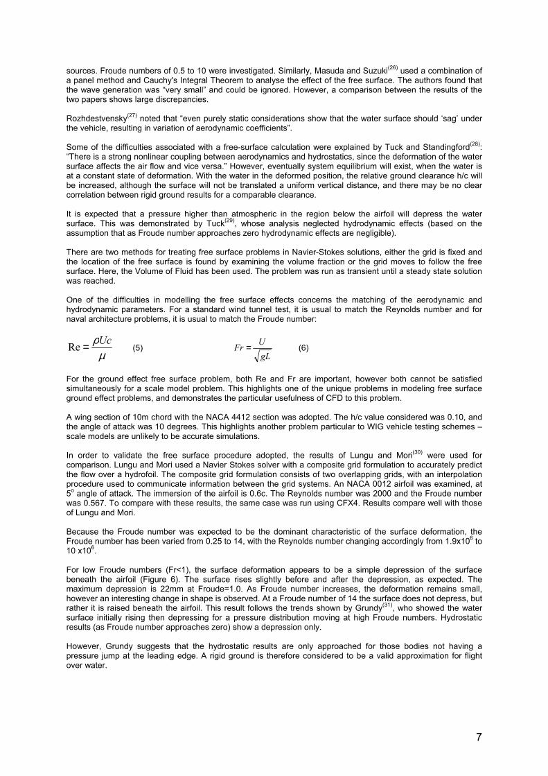
An important effect that can be captured is the effect of the ground condition on the characteristics of the turbulence field. The turbulent kinetic energy can be found by considering the effects of the variance of the velocity fields, which can be expected to have some variation for the two ground conditions. This variation in the turbulent kinetic energy field can be seen in Figure 5.

Figure 5 PIV turbulent kinetic energy a. ground stationary b. ground moving

the central region of the tunnel, for both conditions, the values for the turbulent kinetic energy are fairly low,

n the lower boundary, an obvious difference exists between the two cases. There is a large increase in

Investigation of Effect of Free Surface Deformation

owever, the use of a rigid ground can also be an approximation for the study of vehicles operating over water.

uang and Wong used linearized water wave theory to calculate the free surface resulting from a moving

ataoka et al considered the effect of an airfoil on the free surface and found negligible aerodynamic effects from the resulting deformation. The airfoil was represented by sources and vortices, and the water surface as

0 20 40 60 80 100 X 0 20 40 60 80 100 X

Y 60 40 20 0

Y 60 40 20 0

tke 0.25 0.50 1.0

Inand there is little disturbance to the flow. Near the upper boundary however, the effect of the wall boundary layer can be identified as a region of higher energy, with this effect beginning to be seen from about 10mm from the upper boundary for both cases. Oturbulence on the lower boundary when the ground condition is stationary, while for the case where the ground is moving, there is little variation from the central tunnel region to the boundary.

HThe effect of the aerodynamic pressure on the water surface may also have some influence on the correct boundary conditions to be used.

(23)Hpressure distribution. A constant pressure distribution with rectangular planform was used and free surface displacements were found for Froude numbers of 0.64 and 2.12. Results show good agreement with those of Lamb(24), who first detailed a theoretical approach for calculating the surface waves resulting from a “travelling disturbance”. It is interesting to note the variations in free surface shapes for the two Froude numbers: for low Froude number, surface deformations (at the centreline of the three-dimensional distribution) show significant depression; for the high Froude numbers the surface deformation is minimal, and a small rise is found for the surface beneath the leading edge.

(25)K

6

sources. Froude numbers of 0.5 to 10 were investigated. Similarly, Masuda and Suzuki(26) used a combination of a panel method and Cauchy's Integral Theorem to analyse the effect of the free surface. The authors found that the wave generation was “very small” and could be ignored. However, a comparison between the results of the two papers shows large discrepancies. Rozhdestvensky(27) noted that “even purely static considerations show that the water surface should ‘sag’ under

e vehicle, resulting in variation of aerodynamic coefficients”.

on were explained by Tuck and Standingford(28): here is a strong nonlinear coupling between aerodynamics and hydrostatics, since the deformation of the water

n below the airfoil will depress the water urface. This was demonstrated by Tuck(29), whose analysis neglected hydrodynamic effects (based on the

r the grid is fixed and e location of the free surface is found by examining the volume fraction or the grid moves to follow the free

fficulties in modelling the free surface effects concerns the matching of the aerodynamic and ydrodynamic parameters. For a standard wind tunnel test, it is usual to match the Reynolds number and for

th Some of the difficulties associated with a free-surface calculati“Tsurface affects the air flow and vice versa.” However, eventually system equilibrium will exist, when the water is at a constant state of deformation. With the water in the deformed position, the relative ground clearance h/c will be increased, although the surface will not be translated a uniform vertical distance, and there may be no clear correlation between rigid ground results for a comparable clearance. It is expected that a pressure higher than atmospheric in the regiosassumption that as Froude number approaches zero hydrodynamic effects are negligible). There are two methods for treating free surface problems in Navier-Stokes solutions, eithethsurface. Here, the Volume of Fluid has been used. The problem was run as transient until a steady state solution was reached. One of the dihnaval architecture problems, it is usual to match the Froude number:

ρUc Uµ

=gL

Fr =Re (5) (6)

For the ground effect free surface problem, both Re and Fr are important, however both cannot be satisfied

multaneously for a scale model problem. This highlights one of the unique problems in modeling free surface

dered was 0.10, and e angle of attack was 10 degrees. This highlights another problem particular to WIG vehicle testing schemes –

opted, the results of Lungu and Mori(30) were used for omparison. Lungu and Mori used a Navier Stokes solver with a composite grid formulation to accurately predict

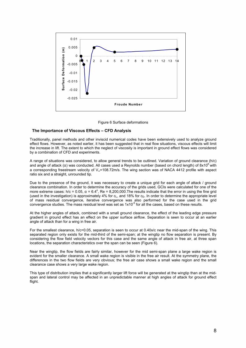
e number was expected to be the dominant characteristic of the surface deformation, the roude number has been varied from 0.25 to 14, with the Reynolds number changing accordingly from 1.9x106 to

roude numbers (Fr<1), the surface deformation appears to be a simple depression of the surface eneath the airfoil (Figure 6). The surface rises slightly before and after the depression, as expected. The

proached for those bodies not having a ressure jump at the leading edge. A rigid ground is therefore considered to be a valid approximation for flight

siground effect problems, and demonstrates the particular usefulness of CFD to this problem. A wing section of 10m chord with the NACA 4412 section was adopted. The h/c value consithscale models are unlikely to be accurate simulations. In order to validate the free surface procedure adcthe flow over a hydrofoil. The composite grid formulation consists of two overlapping grids, with an interpolation procedure used to communicate information between the grid systems. An NACA 0012 airfoil was examined, at 5o angle of attack. The immersion of the airfoil is 0.6c. The Reynolds number was 2000 and the Froude number was 0.567. To compare with these results, the same case was run using CFX4. Results compare well with those of Lungu and Mori. Because the FroudF10 x106. For low Fbmaximum depression is 22mm at Froude=1.0. As Froude number increases, the deformation remains small, however an interesting change in shape is observed. At a Froude number of 14 the surface does not depress, but rather it is raised beneath the airfoil. This result follows the trends shown by Grundy(31), who showed the water surface initially rising then depressing for a pressure distribution moving at high Froude numbers. Hydrostatic results (as Froude number approaches zero) show a depression only. However, Grundy suggests that the hydrostatic results are only appover water.

7

-0.025

-0.02

-0.015

-0.01

-0.005

0

0.005

0.01

0 1 2 3 4 5 6 7 8 9 10 11 12 13 14

Froude Numbe r

Su

rfac

e D

efo

rmat

ion

(m

)

Figure 6 Surface deformations

The Importance of Viscous Effects – CFD Analysis Traditionally, panel methods and other inviscid numerical codes have been extensively used to analyze ground effect flows. However, as noted earlier, it has been suggested that in real flow situations, viscous effects will limit the increase in lift. The extent to which the neglect of viscosity is important in ground effect flows was considered by a combination of CFD and experiments. A range of situations was considered, to allow general trends to be outlined. Variation of ground clearance (h/c) and angle of attack (α) was conducted. All cases used a Reynolds number (based on chord length) of 8x106 with a corresponding freestream velocity of V∞=108.72m/s. The wing section was of NACA 4412 profile with aspect ratio six and a straight, unrounded tip. Due to the presence of the ground, it was necessary to create a unique grid for each angle of attack / ground clearance combination. In order to determine the accuracy of the grids used, GCIs were calculated for one of the more extreme cases: h/c = 0.05, α = 6.4o, Re = 8,200,000.The results indicate that the error in using the fine grid (used in the investigation) is approximately 4% for cL, and 18% for cD. In order to determine the appropriate level of mass residual convergence, iterative convergence was also performed for the case used in the grid convergence studies. The mass residual level was set as 1x10-5 for all the cases, based on these results. At the higher angles of attack, combined with a small ground clearance, the effect of the leading edge pressure gradient in ground effect has an effect on the upper surface airflow. Separation is seen to occur at an earlier angle of attack than for a wing in free air. For the smallest clearance, h/c=0.05, separation is seen to occur at 0.40x/c near the mid-span of the wing. This separated region only exists for the mid-third of the semi-span; at the wingtip no flow separation is present. By considering the flow field velocity vectors for this case and the same angle of attack in free air, at three span locations, the separation characteristics over the span can be seen (Figure 6). Near the wingtip, the flow fields are fairly similar, however for the mid semi-span plane a large wake region is evident for the smaller clearance. A small wake region is visible in the free air result. At the symmetry plane, the differences in the two flow fields are very obvious; the free air case shows a small wake region and the small clearance case shows a very large wake region. This type of distribution implies that a significantly larger lift force will be generated at the wingtip than at the mid-span and lateral control may be affected in an unpredictable manner at high angles of attack for ground effect flight.

8

Turbulent kinetic energy (TKE) in the (entire) flow field is also increased as the ground is approached. The maximum TKE value in the field for the highest incidence investigated (α=10o) increases by 300%, due to the increasing turbulent wake region, as the clearance is lowered from h/c=1.00 to h/c=0.05.

PIV Analysis CFD results have shown that flow separation occurs earlier and that the size of the wake is large, when a wing flies close to the ground. To investigate further this phenomenon, a wing was tested in the tunnel, at high angle of attack and at two clearances. In both cases, the ground moved at the same velocity as the

freestream (15m/s). The Reynolds number for the investigation was 61,000. Although Reynolds numbers effects will cause variation between the CFD and PIV results, the trend as clearance is changed can be reasonably compared. Another advantage of using a combination of both CFD and experiments is highlighted with this variation in Reynolds number – although the wind tunnel tests are not feasible to run at real-life Reynolds numbers, further CFD cases can be run at the same conditions as the wind tunnel and these used to compare to the wind tunnel tests. By validating the CFD at one condition, we can gain confidence in the results at other conditions. Initial tests of the wing test-piece showed that some small regions of poor image resolution were found beneath the leading edge and trailing edge of the wing, due to the light being unable to pass cleanly though these sections of the wing. The wing was set at 12o incidence, and the clearance set at h/c=0.05 and h/c=0.45 above the ground level. A further examination of the effect of the ground on the wake and separation is given in Figure 7, presenting contours of turbulent kinetic energy for the flow fields, showing the area around the trailing edge region, highlighting the energy levels in the wake regions. A comparison of the CFD and PIV results is shown, for both clearances. Significant differences in energy are found in the wake region for the two cases, with the low clearance showing a high-energy region much large than the high clearance. The effect of flying closer to the ground has increased the levels of energy in and the size of the wake region, as

also indicated by the previous CFD results.

Figure 7 TKE contours, trailing edge region. Re=61x103. a. h/c=0.05 b. h/c=0.45

PIV tke CFD tke NACA 4412 wing at 12o, h/c=0.05, trailing edge region

PIV tke CFD tke NACA 4412 wing at 12o, h/c=0.45, trailing edge region

Figure 6 Velocity vectors, α=10o, h/c=0.05 and h/c=free air, Re=8x106

9

Large Moving Ground Design

bility to conduct accurate ground effect experiments is limited to the o-phase PIV tunnel and the open-section tunnel, which utilizes a low-speed moving ground for visualization

er to determine the most appropriate configuration and location of the moving ground for this tunnel, reliminary CFD work has been conducted on a proposed design. The aim of the work was to define the moving

ximately 1.2m wide by 2.2m long and a thickness of .15m. The moving ground will operate up to the same speed as the wind tunnel freestream can be set to of

the existing force balance is located beneath the test section and it is our intention to continue to use it ith the new moving ground, the moving ground has been positioned in the current test section by suspending it.

Contou

Extensive CFD analysis was carrie d be obtained by simply hanging e moving ground in the wind tunnel’s test section. Initial two-dimensional CFD simulations indicated that this

een a vital and integral part of the design process; we expect the moving ground to cause very little disturbance

area of ground effect aerodynamics showed variation in both results and methodology. In particular, the importance of the implementation of boundary conditions and the neglect of

stigate the influences and it was found that a moving ground the only accurate ground boundary condition for body-fixed simulation. It was also shown that the deformable

surface effect (for vehicles flying over water) can be assumed negligible.

At the University of New South Wales, the atwpurposes. The larger, 3ft x 4ft subsonic wind tunnel, capable of speeds up to 60m/s currently only has the option of a stationary ground plane. The design and construction of a moving ground for this tunnel is currently under way. In ordpground that would give the most uniform profile across the test section, for both velocity and, importantly, turbulence levels, before the construction even begins. The overall dimensions of the moving ground are appro060ms-1. Because wIn order for the moving ground to be successful, it would have to provide a physical boundary that has no boundary layer forming over it. It would also have to have as little effect as possible on the turbulence in the wind tunnel test section.

40

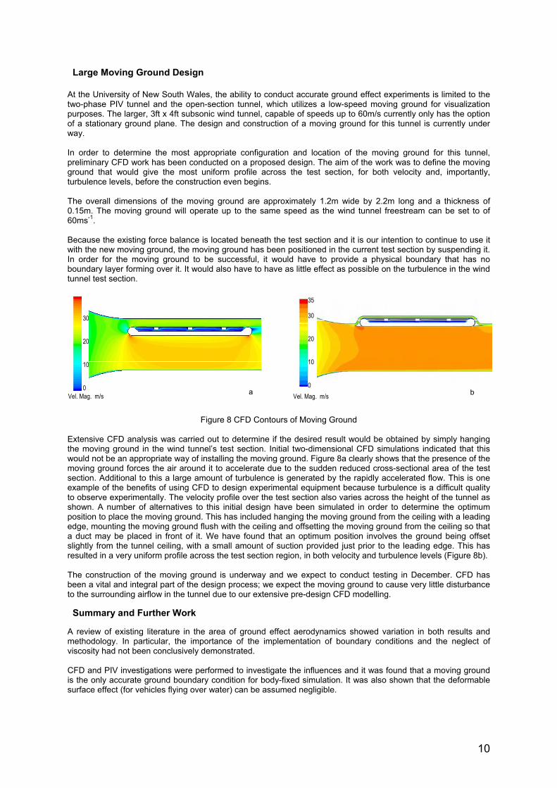
Figure 8 CFD

30 20 10 0

Vel. Mag. m/s a

rs of Moving Ground

30 20 10 0

Vel. Mag. m/s

35

b

d out to determine if the desired result woul

thwould not be an appropriate way of installing the moving ground. Figure 8a clearly shows that the presence of the moving ground forces the air around it to accelerate due to the sudden reduced cross-sectional area of the test section. Additional to this a large amount of turbulence is generated by the rapidly accelerated flow. This is one example of the benefits of using CFD to design experimental equipment because turbulence is a difficult quality to observe experimentally. The velocity profile over the test section also varies across the height of the tunnel as shown. A number of alternatives to this initial design have been simulated in order to determine the optimum position to place the moving ground. This has included hanging the moving ground from the ceiling with a leading edge, mounting the moving ground flush with the ceiling and offsetting the moving ground from the ceiling so that a duct may be placed in front of it. We have found that an optimum position involves the ground being offset slightly from the tunnel ceiling, with a small amount of suction provided just prior to the leading edge. This has resulted in a very uniform profile across the test section region, in both velocity and turbulence levels (Figure 8b). The construction of the moving ground is underway and we expect to conduct testing in December. CFD has bto the surrounding airflow in the tunnel due to our extensive pre-design CFD modelling.

Summary and Further Work

A review of existing literature in the

viscosity had not been conclusively demonstrated. CFD and PIV investigations were performed to inveis

10

CFD and PIV investigations were conducted to investigate specific characteristics of the flow that would only be present in a viscous analysis. Viscous effects were found to be significant for ground effect flight and it is

erefore unlikely that inviscid solutions give an accurate representation of ground effect aerodynamics.

Bibliography

th The CFD analysis of a 60m/s moving ground design for the UNSW 3ft x 4ft wind tunnel was shown as a further example of the integration of CFD and experimentation, in the study of ground effect aerodynamics.

1 of a Workshop on Twenty-First Flying Ships, The University of New South Wales, Nov

7-8, 1995. Institute of Marine Engineers, Sydney. 2 Prandolini, L. 1996 Workshop Proceedings of Ekranoplans And Very Fast Craft, The University of New South

3 To Ekranoplan GEMs, The University of New South

4 t: A Very-High-Speed Catamaran with

).

6 of Wings Near Ground”. Trans.Japan

, A., Younger, S., and Roberts, T. 1997 “Aerodynamics of High-Speed Multihull Craft”.

9 Park, I. 1995 “Analysis of Steady and Unsteady Performance for 3D Airwing in Vicinity of Free

11 5 Numerical Investigation of the Thickness and Camber Effects on Aerodynamic

iences (38) 119. pp.77-90.

13 M 77.

p.631-638. nel. Proc. 6th Colloq. on Industrial

16 round Simulation on the Flow Around Vehicles

17 Rev.Fluid Mech. 25. pp.485-537.

NACA

20 rification and Validation in Computational Science and Engineering. Hermosa Publishers,

21 dama, Y. 1995 Flow Computation for 3D Wing in Ground Effect using Multi-Block Technique.

22 . 2001 Investigation of Two-Phase Backward Step Flow with Electrostatics. University of New South

23 Distribution Moving over a Free Surface.

24 dynamics. Cambridge University Press, UK.

1-30. ects of Two-Dimensional WIG Moving Near

the Free Surface. Journal of the Society of Naval Architects of Japan (170) pp.83-92.

Prandolini, L. 1995 Proc.

Wales, 5-6 December, 1996. Institute of Marine Engineers, Sydney. Prandolini, L. 1998 Workshop Proceedings of WISE UpWales, 15-16 June, 1998. Institute of Marine Engineers, Sydney. Doctors, L.J. 1997 “Analysis of the Efficiency of an EkranocaAerodynamic Alleviation”, Proc. International Conference on Wing-in-Ground-Effect Craft (WIGs '97), Royal Institution of Naval Architects, London, England, 16 pp (Dec. 1997

5 Zerihan, J. and Zhang, X. 2001 “Aerodynamics of Gurney Flaps on a Wing in Ground Effect”. AIAA Journal 39(5). pp 772-780. Steinbach, D. and Jacob, K. 1991 “Some Aerodynamic AspectsSoc.Aeronautical and Space Sciences (34) 104. pp.56-70.

7 Walker, G., FougnerFourth International Conference on Fast Sea Transportation (FAST97). July 21-23, 1997. Sydney, Australia., pp.133-138.

8 Rozhdestvensky, K. 1992 Matched Asymptotics in Aerodynamics of WIG Vehicles. Intersociety High Performance Marine Vehicle Conference and Exhibit, pp.WS17-WS27. Chun, H. andSurface.” Proceedings of a Workshop on Twenty-First Century Flying Ships, University of New South Wales, December 1996. pp.23-46.

10 Katz, J. 1985 “Calculation of the Aerodynamic Forces on Automotive Lifting Surfaces.” Journal of Fluids Engineering 107. pp.438-443. Hsiun, C. and Chen, C. 199Characteristics for Two-Dimensional Airfoils With Ground Effect in Viscous Flow. Trans.Japan Soc.Aeronautical and Space Sc

12 Steinbach, D. 1997 Comment on "Aerodynamic Characteristics of a Two-Dimensional Airfoil with Ground Effect". AIAA Journal of Aircraft (34) 3. pp.455-456. Wieselsberger, C. 1922 Wing Resistance Near the Ground. NACA T

14 George, A. 1981 Aerodynamic Effects of Shape, Camber, Pitch and Ground Proximity on Idealized Ground Vehicle Bodies. Journal of Fluids Engineering 103. p

15 Diuzet, M. 1985 The Moving Belt of the IAT Long Test Section Wind TunAerodynamics, June 1985, Road vehicle aerodynamics., pp.159-167. Fago, B., Lindner, H., and Mahrenholtz, O. 1991 The Effect of Gin Wind Tunnel Testing. J.Wind Eng.and Ind.Aerodynamics (38) pp.47-57. Hucho, W. and Sorvan, G. 1993 Aerodynamics of Road Vehicles. Ann.

18 Zerihan, J. and Zhang, X. 2001 Aerodynamics of Gurney Flaps on a Wing in Ground Effect. AIAA Journal 39(5). pp 772-780.

19 Pinkerton, R. 1938 The Variation with Reynolds Number of Pressure Distribution over an Airfoil Surface. Report No. 613. Roache, P.1998 VeUSA. Hirata, N. and KoJournal of the Society of Naval Architects of Japan (177) pp.49-57. Hall, SWales. PhD Thesis. Huang, T. and Wong, K. 1970 Disturbance Induced by a PressureJournal of Ship Research (14) 3. pp.195-203. Lamb, H.1932, Hydro

25 Kataoka, K., Ando, J., and Nakatake, K. 1991 Free Surface Effects On Characteristics Of 2D Wing. Trans.of the West Japan Soc.Naval Architects (83) pp.2

26 Masuda, S. and Suzuki, K. 1991 Simulation of Hydrodynamic Eff

11

s, Nov 7-8, 1995, pp.47-70.

10.

27 Rozhdestvensky, K. 1995 Ekranoplans - Flying Ships Of The Next Century. Proc. of a Workshop on Twenty-First Flying Ships, The University of New South Wale

28 Tuck, E. and Standingford, D. 1996 Lifting Surfaces In Ground Effect. Workshop Proceedings of Ekranoplans and Very Fast Craft, University of New South Wales, 5-6 Dec, 1996. pp.230-243.

29 Tuck, E. 1984 A Simple One-Dimensional Theory for Air-Supported Vehicles Over Water. Journal of Ship Research (28) 4. pp.290-292.

30 Lungu, A. and Mori, K. 1994 Applications of Composite Grid Method for Free-Surface Flow Computations by Finite Difference Method. Journal of the Society of Naval Architects of Japan (175) pp.1-

31 Grundy, I. 1986 Airfoils Moving in Air Close to a Dynamic Water Surface. J.Australian Math.Soc. (Series B 27) 3. pp.327-345.

12