Advances in Political Economy:Institutions, Modelling and Empirical

analysis

Norman Scho�eld, Gonzalo Caballero and Daniel Kselman

September 28, 2012

1 Contents

ContributorsIntroductionNorman Scho�eld, Gonzalo Caballero and Daniel KselmanPart I: InstitutionsTransaction Cost Politics in the map of the New Institutionalism

by Gonzalo Caballero and Xose Carlos Arias.Political Transitions in Medieval Venice and Ancient Athens: An

Analytical Narrative by Leandro de Magalhaes.A Collective-Action Theory of Fiscal-Military State Building by

Luz Marina AriasStable Constitutions in Political Transition byGerald Pech, and Katja

MichalakQuandaries of Gridlock and Leadership in U.S.Electoral politics by

Norman Scho�eld and Evan Schnidman.Sub-central Governments and Sovereign Debt crisis in Spain over

the Period 2000-2011 by Fernando TobosoDeciding How to Choose the US Healthcare System byOlga Shvetsova

and Katri SiebergPart II: ModellingChallenges to the Standard Euclidean Spatial Model by Jon EguiaA Non-Existence Theorem for Clientelism in Spatial Models by

Daniel KselmanNonseparable Preferences and Issue Packaging in Elections by Dean

Lacy and Emerson NiouWhen will insider candidates avoid a primary challenge? A model

of partial revelation of information by Gilles SerraMeasuring the Latent Quality of Precedent: Scoring Vertices in a

Network by John W. Patty, Elizabeth Maggie Penn, and Keith E. Schnaken-berg

1

Part III Empirical analysisThe Politics of Austerity: Modelling British Attitudes Towards

Public Spending Cuts: by Harold Clarke, Marianne Stewart, David Sanders,andPaul Whiteley.

Modelling Elections with Varying Party Bundles: An Applicationto the 2004 Canadian Election by Kevin McAlister, Jee Seong Jeon andNorman Scho�eld,A Spatial Model of Elections in Turkey: Tracing Changes in the

Party System in the 2000s by Norman Scho�eld and Betul DemirkayaDo Competitive Districts Necessarily Produce Centrist Politicians?

by James Adams, Thomas L. Brunell, Bernard Grofman and Samuel Merrill,III.A Heteroscedastic Spatial Model of the Vote: A Model with Appli-

cation to the United States by Ernesto Calvo, Timothy Hellwig and KiyoungChang.Inferring Ideological Ambiguity from Survey Data, by Arturas RozenasBiographies

2

ContributorsJames Adams, Department of Political Science, UC Davis, Davis, CA

95616, USA.<jfadams@ucdavis.edu>.Luz Marina Arias ,CEACS, Juan March Institute, C/Castello 77, Madrid

28006, Spain. <larias@march.es>Xose Carlos Arias, Faculty of Economics, Campus As Lagoas-Marcosende,

University of Vigo, 36310 Vigo,Spain.<xcarias@uvigo.es>Thomas L. Brunell, Senior Associate Dean of Graduate Education, School

of Economic, Political and Policy Science,UT Dallas 800 W. Campbell Road,Richardson, TX 75080, USAGonzalo Caballero Faculty of Economics, Campus As Lagoas-Marcosende,

University of Vigo, 36310 Vigo,Spain.<gcaballerom@yahoo.com>Ernesto Calvo University of Maryland,Government and Politics, 3144F

Tydings Hall, College Park MD 20742 USA.<ecalvo@umd.edu>Kiyoung Chang 9348 Cherry Hill Road #713, College Park MD 20740.

USAHarold Clarke,School of Social Science, PO Box 830688, University of

Texas at Dallas, Richardson. TX 75083-0688,<hclarke@utdallas.edu>Leandro De Magalhaes, Department of Economics, University of Bristol,

8 Woodland Road, Bristol BS8 1TN, UK <leandro.magalhaes@bristol.ac.uk>Betul Demirkaya, Center in Political Economy, Washington University in

Saint Louis, 1 Brookings Drive, Saint Louis, MO 63130,USA.<betul.demirkaya@wustl.edu>Jon Eguia, Department of Politics, New York University, 19 West 4th

street, New York, NY 10012 USA. <equia@nyu.edu>Bernard Grofman School of Social Sciences, University of California,

SSPB 5215, Irvine, CA 92697-5100, USA.<bgtravel@uci.edu>Timothy Hellwig Department of Political Science,Indiana University,Woodburn

Hall 210,1100 E Seventh Street, Bloomington IN 47405-7110. USA.<thellwig@indiana.edu>Jee Seong Jeon, Center in Political Economy, Washington University in

Saint Louis, 1 Brookings Drive, Saint Louis,MO 63130, USA.<jsjeon@wustl.ed·u>Dan Kselman Center for Advanced Studies in the Social Sciences, Juan

March Institute C/Castello 77, 28006 Madrid, Spain.<dkselman@march.es>Dean Lacy Dartmouth College, HB 6108, Hanover, NH 03755, USA.<Dean.P.Lacy@dartmouth.edu>Kevin McAlister, Center in Political Economy, Washington University in

Saint Louis, MO 63130, USA.<kevinmcalister@wustl.edu>Samuel Merrill, III. 3024 43rd Ct. NW., Olympia, WA 98502, USA.<sammerrill3@comcast.net>Katja Michalak, Department of Public Management and Governance,Zeppelin

University,Am Seemooser Horn 20, 88045 Friedrichshafen,Germany.<katja.michalak@zu.de>

3

Emerson Niou Department of Political Science, Duke University, 503Perkins Library, Durham, NC 27708-0204. USA.<niou@duke.edu>John W Patty, Center in Political Economy, Washington University in

Saint Louis,1 Brookings Drive, Saint Louis, MO 63130, USA.<jwpatty@gmail.com>Gerald Pech, Department of Economics, KIMEP University, Abay 2, 050010

Almaty, Republic of Kazakhstan.<gp@geraldpech.net>Elizabeth Maggie Penn, Center in Political Economy, Washington Uni-

versity in Saint Louis, 1 Brookings Drive, Saint Louis, MO 63130, USA<elizabeth.m.penn@gmail.com>Arturas Rozenas. Department of Political Science, Duke University,

Durham, NC 27708-0204. USADavid Sanders, Department of Government, University of Essex Colch-

ester C043SQ, UK.<sanders@essex.ac.uk>Keith.Schnakenberg Center in Political Economy, Washington University

in Saint Louis, 1 Brookings Drive, Saint Louis, MO 63130, USA.<keith.schnakenberg@gmail.com>Evan Schnidman. 11 Vandine Street #2,Cambridge, MA 02141, USA

<evan.schnidman@gmail.com>Norman Scho�eld Weidenbaum Center, Washington University in St.

Louis, Seigle Hall, Campus Box 1027, One Brookings Drive,St. Louis, MO63130-4899 USA.<scho�eld.norman@gmail.com>Gilles Serra Political Science Department, Center for Economics Research

and Teaching (CIDE), Lomas de Santa Fe, Mexico City 01210, Mexico.<gilles.serra@cide.edu>Olga Shvetsova, Department of Political Science, Binghamton University,

P.O. Box 6000, Binghamton, NY 13902, USA.<shvetsova@gmail.com>Katri Sieberg, Department of North American Studies, University of Tam-

pere 33104, Tampereen Yliopisto, Finland.<katri.sieberg@uta.�>Marianne Stewart, School of Social Science, PO Box 830688, University

of Texas at Dallas, Richardson. TX 75083-0688,USA< mstewart@utdallas.edu>FernandoToboso Faculty of Economics, Departamento de Economía Apli-

cada, Av. Tarongers s/n, University of Valencia, 46022 Valencia, Spain.<Fernando.Toboso@uv.es>Paul Whiteley Department of Government, University of Essex Colchester

C043SQ, UK. <whiteley@essex.ac.uk>.

4

1.1 Introduction

Norman Scho�eld, Gonzalo Caballero and Dan KselmanPolitical Economy is both a growing �eld and a moving target. The con-

cept �political economy� remains something of an open signi�er, alternativelyused to describe a methodological approach in political analysis, grounded inthe application of formal and quantitative methods to the study of politics; orone of any number substantive areas in the contemporary social sciences. Ineconomics, new institutional economics (Willimason 1985, North 1990) has es-tablished the fundamental importance of history- and polity-speci�c governancestructures in sustaining economic markets. Comparative research has investi-gated the e¤ect of democratic institutions and processes on economic policyand outcomes, research given perhaps its most comprehensive statement in inPersson and Tabellini (2000) and Drazen (2001), which have constituted the so-called �macroeconomics side�of political economy (Merlo, 2006). Developmenteconomists increasingly recognize that, absent sound governance institutions,standard macroeconomic prescriptions for economic growth and stability oftenfail to bear fruit (Rodrik, 2007). Economists have also recently joined politi-cal scientists in examining the role of economic factors in explaining democratictransitions and the evolution of political regimes (Acemoglu and Robinson 2000,2006). Dewan and Shepsle (2008) have emphasized that in recent years someof the best theoretical work on the political economy of political institutionsand processes has begun surfacing in the political science mainstream, and theyconsider that this is a result of economists coming more �rmly to the conclusionthat modeling governments and politicians is central to their own enterprise.Moving to political science, work on the modernization hypothesis, moti-

vated by the consistently high cross-national correlation between democraticconsolidation and economic development, has also recognized the role of eco-nomic factors in determining the evolution of political regimes (Moore 1965;O�Donnell 1974; Przeworski et al. 2000). Furthermore, comparative politicalscience in many ways beat economics to the punch in recognizing the role thatpolitical institutions play in determining the economic trajectories of developingand still industrializing economies (Haggard and Kaufmann 1990). Economicclass structures, and their embodiment in labor unions and professional orga-nizations, have occupied an important place in comparative politics researchon the economic institutions of advanced industrial societies ( Hall and Soskice2001). Studies of voter behavior have identi�ed both the role that conjunturaleconomic factors play in informing voter choice and the relationship betweenvoters� professional context and their preferences for redistribtuion . As al-ready mentioned, the label political-economy also refers more loosely to theapplication of formal and game theoretic methods �rst developed by economiststo the study of political phenomena, including legislative bargaining (Shep-sle 1979; Krehbiel 1998), government coalition formation (Laver and Scho�eld1990; Laver and Shepsle 1996), and campaign position-taking (Cox 1987, 1990;Scho�eld 2006).In this sense, the e¤ect of economics has been felt more stronglyin contemporary political science than any other social science (Miller, 1997).

5

As evidenced by this brief, and necessarily incomplete, literature review,political economy is a concept with fairly �exible boundaries, encompassing re-search from a wide variety of �elds and approaches. For example, Weingastand Wittman (2008) viewed political economy as the methodology of economicsapplied to the analysis of political behavior and institutions, but they assumedthat it is not a single approach because it consists of a family of approaches.Previously, two views had been distinguished in the new political economy, andboth have contributed to the advance of the understanding of modern politicaleconomy: on the one hand, Hamiltonian political economy has been interestedin economic patterns and performance, but it considers that political institu-tions and political choices are relevant explaining factors; on the other hand,Madisonian political economy has assumed that the economic approach is cen-tral in political analysis, quite apart from economic content (Shepsle, 1999).Rather than an explicit ��eld� or �discipline� in and of itself, the notion ofpolitical economy represents rather a growing awareness in both political sci-ence and economics that their respective contributions to our understanding ofsociety are intelligible only in mutual conversation. It is one thing for scholarsin both disciplines to recognize the interdependence of their subject matters; itis another to create professional fora in which practitioners of these two disci-plines come together. The current volume results from the latest in a series ofconferences designed to engender a closer collaboration between economists andpolitical scientists. Its contributions represent a broad spectrum of research,and its contributors a diverse group of scholars from diverse academic tradi-tions in political economy. Nonetheless, as a group we share a commitment tomutually bene�cial interdisciplinary collaboration, such it has been shown inprevious e¤orts (Scho�eld and Caballero, 2011).These conferences took place in April and May of 2012. The �rst was held

at the Juan March Institute in Madrid, Spain, and was entitled Contempo-rary Applications of the Spatial Model. Ever since Downs�seminal work (1957),the spatial model has been a workhorse in formal political theory. While itscore content addresses how parties choose the relative extremism or moderationof campaign positions, its results have also been used in studies of economicpolicy and redistribution (Meltzer and Richard 1978; Persson and Tabelinni2000). The Madrid conference brought together a group of leading scholarsworking on contemporary applications of the spatial paradigm, including theo-retical contributions on spatial consequences of primary elections and the spatialconsequences of vote buying; and empirical contributions on the measurementof parties actual policy positions, the extent to which voters accurately perceivesuch positions, and how these pereceptions are moulded by voters� ideologcalpredispositions.The second conference was held in Baiona, Spain, and supported by the

Erenea Research Group at the University of Vigo, and the Center in PoliticalEconomy at Washington University in Saint Louis.. This conference was in factthe second installment of the International Conference on Political Economyand Institutions (ICOPEAI); and like the �rst, which was held in June 2010, itbrought together political scientists and economists from many countries. The

6

spatial model featured prominently in Baiona as well; but to this agenda wasadded a variety of papers on political transitions, democratic performance andhuman capital formation, social networks, and new insitutional economics, andvoting.There was substantial overlap in the participants at both conferences, al-

lowing for a fruitful extended dialogue that,along with an internal peer-reviewprocess, has improved the content of the volume�s contributions.The editors thank the University of Vigo, the Juan March Institute, and

the Center in Political Economy, Washington University in Saint Louis for thesupport they provided.We have decided to structure the volume in three sections, each dealing with

a particular emphasis in political economic research: Institutions, Modeling, andEmpirical Analysis.Each chapter in this book went through a review process before publication.

These chapters deal with theoretical and empirical issues over the the behaviorof institutions and the operation of democratic elections. Below we give theabstracts of the topics discussed in these chapters.

7

2 Abstracts

2.1 Part 1: Institutions

1.: �Transaction Cost Politics in the map of the New Institutionalism�by Gon-zalo Caballero and Xose Carlos Arias . In recent decades, the new institutional-ism has strongly emerged in social sciences. Institutions have come back to themain research agenda in economics, politics and sociology. This paper presentsand analyses the program of Transaction Cost Politics within the map of thenew institutionalism. Transaction Cost Politics constitutes an extension of theNew Institutional Economics towards the analysis of politics, and it points outthe relevance of institutions in political markets that are characterized by incom-plete political rights, imperfect enforcement of agreements, bounded rationality,imperfect information, subjective mental models on the part of the individualsand high transaction costs. The paper reviews the main contributions of Trans-action Cost Politics and we study the relationships of Transaction Cost Politicswith Rational-Choice Institutionalism, Constitutional Political Economy andthe New Institutional Economics.2. Political Transitions in Medieval Venice and Ancient Athens by Leandro

de Magalhaes.Models of political transitions have mostly focused on the 19th and 20th

centuries. Their setup tends to be speci�c to the contemporary period. ThisChaper reviews the events that led to democracy in ancient Athens and to ruleby council in medieval Venice. We confront the available models of politicaltransition with these events. We �nd evidence that war and economic conditionsplayed a key role. The political economy models that incorporate these featuresdo well in explaining the transitions in both ancient Athens and medieval Venice.3. A Collective-Action Theory of Fiscal-Military State Building by Luz Ma-

rina AriasPrior to the emergence of the �scal-military state, many monarchs depended

on economic and local elites for the collection of tax revenue and defense. Whydid these powerful elites allow the ruler to increase �scal centralization andbuild-up militarily? Building on historical accounts of colonial Mexico and 17thcentury England, This chapter develops a game-theoretic analysis that explainswhy increases in �scal centralization are more likely when the probability of athreat of internal unrest or external invasion increases. Elites free ride on �s-cal contributions under fragmented �scal capacity. Centralized �scal collectionand enforcement serves as an institutional devise for the elites to overcome freeriding and ensure the provision of military protection. The analysis shows thatan increase in the probability of a threat is more likely to result in central-ization when the alignment between the elites�and the ruler�s vulnerability tothe threat is high, and in the presence of economic growth. The analysis alsosuggests that institutions that allow rulers to commit, such as representative as-semblies, may not be necessary for �scal centralization to transpire. Examplesfrom European and colonial history provide support for the implications of thetheoretical analysis.

8

4: Stable Constitutions in Political Transition by Gerald Pech and KatjaMichalakThis chapter develops a spatial model where an autocrat selects a status quo

constitution which a succeeding elected constitutional assembly may or may notaccept as a blue print for negotiations on constitutional reform. If the autocratexpects that the future constitutional assembly is dominated by parties whichfavor redistribution, he does not want to bind himself by the constitution. If themiddle-class opposes redistribution or the middle class and the right dominatethe constitutional assembly, stable constitutions exist which are in the interestof the autocrat. This framework is applied to transition processes in Chile andEgypt.5. Quandaries of Gridlock and leadership in U.S. Electoral politics by Nor-

man Scho�eld and Evan Schnidman.In 1964 President Johnston was able to overcome Southern Democrat op-

position to the Civil Rights legislation. Recent opposition by Republicans inCongress has induced a form of legislative gridlock, similar to the situation fac-ing Johnston. This paper argues that the current gridlock is more perniciousthan in 1964 for two reasons. The pivot line in the two dimensional policyspace has shifted slightly so that voters are more clearly separated by di¤erentpreferences on civil rights. Secondly the era of deregulation since the electionof Reagan has brought money into the political equation, especially since Citi-zen�s United decision of theSupreme Court. The argument is based on a formalmodel of the 2008 election and shows that excluding money, both candidatesin 2008 would have adopted centrist positions. We argue that it was moneythat pulled the candidates into opposite quadrants of the policy space.We sug-gest that the same argument holds for members of Congress. leading to to thecurrent gridlock. Before discussing the current gridlock between the executiveand legislative arms of government we draw some parallels with earlier episodesin US political history, particularly the early years of the Roosvelt presidencyand the leade-up to the passage of the Civil Rights legislation in 1964. We alsosuggest that in fragmented or multiparty systems, based on proportional repre-sentation, such as in the euro area,small parties will adopt radical policies farfrom the electoral center, thus inducing coalition instability. This phenomenoncoupled with a fragile �scal system based on the euro also has created di¢ cultiesin dealing e¤ectively with the fall-out from the recession of 2008-9.6.Sub-central governments and sovereign debt crisis in Spain over the period

2000-2011 by Fernando Toboso.This chapter studies the quantitative evolution of sub-central sovereign debt

in Spain over the period 2000-2011 and compares it with the evolution of cen-tral debt. As an intense process of political and �scal decentralization has takenplace since the mid eighties, the paper examines whether this drive to decentral-ization has been paralleled by any �scally undisciplined behavior on the part ofSpanish sub-central governments over the period considered. Some key formallegal rules and informal behavioral norms present at sub-central politics in Spainare examined, including legal controls on borrowing by sub-central governments.The empirical analysis will be based on the internationally comparable public

9

�nance �gures provided by sources such as the OECD, the Eurostat and theBank of Spain. The paper concludes that economic performance seem to bethe key factor for explaining the evolution of sub-central, as well as central,public debt before and after the world �nancial crash. The analysis shows thatin terms of the Spanish GDP the debt burden generated by sub-central gov-ernments in Spain decreased over the 2000-2007 period. However, this debthas soared from 8.5 per cent of Spanish GDP in 2007 to 16.4 per cent in 2011,adding 85 thousand millions euros (about 106 billions US dollars) to the stockof total public debt in Spain in just four years. Central government added 267thousand millions euros (about 334 billions US dollars)..7. Deciding How to Choose the U.S. Healthcare System Olga Shvetsova and

Katri SiebergThe continuing debate in the United States over the form of health care

provision is illustrative as to how di¢ cult that choice can be. The choice isfurther complicated by political activity � lobbyists with a vested interest invarious formats � and a noticeable e¤ect from path dependence � people areused to what they have and are afraid of change, and some groups actuallystand to lose from change, at least in the short run. What might the decisionhave been in the absence of these e¤ects? This chapter creates a model to explorethis question. In particular, we appeal to insights from Buchannan and Tullock(1962), Rawls (1971) and Kornai and Eggleston(2001) to ask what type of healthcare provision would a polity choose from behind the veil of ignorance, and whattype of mechanism �unanimity (constitutional) or majority (legislative) wouldthey prefer to use to select it?

2.2 Part 2 Modelling

8.: Challenges to the standard Euclidean spatial model by Jon EguiaSpatial models of political competition over multiple issues typically assume

that agents�preferences are represented by utility functions that are decreasingin the Euclidean distance to the agent�s ideal point in a multidimensional policyspace. I describe theoretical and empirical results that challenge the assumptionthat quasiconcave, di¤erentiable or separable utility functions, and in particu-lar linear, quadratic or exponential Euclidean functions, adequately representmultidimensional preferences, and I propose solutions to address each of thesechallenges.9. A Non-Existence Theorem for Clientelism in Spatial Models by Dan Ksel-

man.This chapter proposes a spatial model that combines both programmatic as

well as clientelistic modes of vote-seeking. In the model political parties strate-gically choose: (1) their programmatic policy position, (2) the e¤ort they devoteto clientelism as opposed to the promotion of their programmatic position, and(3) the set of voters who are targeted to receive clientelistic bene�ts. I presenta theorem which demonstrates that, in its most general form, a spatial modelwith clientelism yields either Downsian convergence without clientelist target-ing, or an ini�nite cycle. Put otherwise, in its most general form the model

10

never yields a Nash Equilibrium with positive levels of clientelism. I relate thisresult to past research on instability in coalition formation processes, and thenidentify additional restrictions, regarding voter turnout and the set of voterswhich parties can target, which serve to generate Nash equilibria with positiveclientelist e¤ort.10. Nonseparable Preferences and Issue Packaging in Elections by Dean

Lacy and Emerson NiouIn this chapter we develop a model in which candidates have exogenously

�xed positions on a single issue dimension on which one candidate has an ad-vantage by being closer to the median voter. The disadvantaged candidate canintroduce a new issue to win the election. When all voters have separable pref-erences and the advantaged candidate moves last on the new issue, there is noway for the disadvantaged candidate to win. When some voters have nonsepa-rable preferences over the issues, the disadvantaged can take a position that theadvantaged candidate cannot beat. Candidates in an election can bene�t fromintroducing new issues, but only when some voters have nonseparable prefer-ences. Using data from a 2004 survey, we show that a substantial percentageof US voters have nonseparable preferences for many issues of public policy,creating incentives and opportunities for political candidates to package issues.11. When will insider candidates avoid a primary challenge? A model of

partial revelation of information by Gilles Serra.When can a party insider feel safe from an outside challenge for a future

nomination? In most countries, parties can choose whether to hold a primaryelection where the rank-and-�le members take a vote, or to allow party leadersto directly appoint an insider candidate of their liking. The cost of primariesforces candidates to drift away from the party leader�s policy preferences inorder to cater to primary voters. This paper postulates a bene�t: primary elec-tions can reveal information about the electability of potential candidates. Ire�ne the formal model in Serra (2011) by making the realistic assumption thatsuch information is revealed partially rather than fully. A signaling mechanismis introduced whereby candidates send noisy information that is used by pri-mary voters to update their beliefs. This leads to surprising insights about thebehavior of primary voters: under some circumstances they will use the informa-tion provided by primary campaigns, but under other circumstances, they willchoose to completely ignore such information. In addition, the results predictthat popular incumbents will not be challenged in a primary election, which isconsistent with empirical observation. Finally, a prescription for parties is toallow their primaries to be tough given that sti¤ competition will improve theexpected ability of the nominee.For intermediate values in the parameters, parties have multiple equilibria in

their decision to adopt primaries or not. And �nally, parties display a signi�cantdegree of contagion, meaning that a party�s adoption of a primary will in�uencethe other party to adopt a primary as well12. Measuring the Latent Quality of Precedent: Scoring Vertices in a Net-

work by John W. Patty, Elizabeth Maggie Penn, and Keith E. Schnakenberg.In this chapter, we consider the problem of estimating the latent in�uence

11

of vertices of a network in which some edges are unobserved for known reasons.We present and employ a quantitative scoring method that incorporates di¤er-ences in �potential in�uence�between vertices. As an example, we apply themethod to rank Supreme Court majority opinions in terms of their �citability,�measured as the likelihood the opinion will be cited in future opinions. Ourmethod incorporates the fact that future opinions cannot be cited in a present-day opinion. In addition, the method is consistent with the fact that a judicialopinion can cite multiple previous opinions..

2.3 Part 3 Empirical analysis

13. The Politics of Austerity: Modelling British Attitudes Towards PublicSpending Cuts:by Harold Clarke, David Sanders, Marianne Stewart, and PaulWhitely.The fallout from the 2008 �nancial crises has prompted acrimonious national

debates in many Western democracies over the need for substantial budget cuts.Among economic and political elites there is broad agreement that substantialpublic sector budget cuts are necessary to address unsustainable sovereign debtand to establish long-term �scal integrity. Many ordinary citizens see things dif-ferently, since austerity measures threaten programs that challenge longstandingpublic commitments to education, health and personal security that constitutethe foundation of the modern welfare state. We investigate the nature of publicattitudes towards the budget cuts using surveys from the British Election Study.The results suggest that cuts currently are widely perceived by the public asessential for Britain�s long-term economic health. But an upward trending viewthat slashing public services will cause serious di¢ culties for families may leadmany people eventually to say enough is enough. It is likely that support forthe cuts will be undermined by a lack of visible results in the real economy.14. Modelling Elections with Varying Party Bundles: An Application to the

2004 Canadian Election by Kevin McAlister, Norman Scho�eld, and Jee SeongJeon.Previous models of elections have emphasized the convergence of parties to

the center of the electorate in order to maximize votes received. More recentmodels of elections demonstrate that this need not be the case if asymmetry ofparty valences is assumed and a stochastic model of voting within elections isalso assumed. This model seems able to reconcile the widely accepted medianvoter theorem and the instability theorems that apply when considering multi-dimensional policy spaces. However, these models have relied on there being asingular party bundle o¤ered to all voters in the electorate. In this paper, weseek to extend these ideas to more complex electorates, particularly those wherethere are regional parties which run for o¢ ce in a fraction of the electorate. Wederive a convergence coe¢ cient and out forth necessary and su¢ cient conditionsfor a generalized vector of party positions to be a local Nash equilibrium; whenthe necessary condition fails, parties have incentive to move away from thesepositions. For practical applications, we pair this �nding with a microeconomet-

12

ric method for estimating parameters from an electorate with multiple regionswhich does not rely on independence of irrelevant alternatives but allows esti-mation of parameters at both aggregate and regional levels. We demonstratethe e¤ectiveness of this model by analyzing the 2004 Canadian election.15.A Spatial Model of Elections in Turkey: Tracing Changes in the Party

System in the 2000s by Norman Scho�eld and Betul DemirkayaThe Turkish political party system underwent signi�cant changes during the

�rst decade of the 21st century. While secularism and nationalism remainedthe de�ning issues of electoral politics, both the number and the ideologicalpositions of parties in the political system changed considerably. In the 2002elections, none of the parties from the previous parliament were able to passthe electoral threshold. The new parliament was formed by the members ofthe Justice and Development Party (AKP)� a new conservative party foundedby the former members of Islamist parties� and the Republican People�s Party(CHP)� a party with a strong emphasis on a secularist agenda. In the 2007elections, AKP consolidated their power by receiving 46.6% of the votes whileCHP increased their share of the vote by only 1.5 percentage points to 20.9%.In addition, the Nationalist Action Party (MHP) and independent candidatessupported by the pro-Kurdish Democratic Society Party (DTP) were able to winseats in the 2007 elections. In order to explain these changes, this paper appliesthe spatial model to the 2007 elections and compares the results to previousanalyses of the 1999 and 2002 elections (Scho�eld et al. 2011b). First, we run apure spatial model to estimate the relative role of the ideological position andthe valence of political parties in determining their electoral success. Second,we supplement the spatial model with the demographic characteristics of voters.Finally, we use simulations to determine whether a Nash equilibrium exists forthe position of political parties or candidates.16. Do Competitive Districts Necessarily Produce Centrist Politicians? by

James Adams, Thomas L. Brunell, Bernard Grofman and Samuel Merrill, IIIUsing the �rst dimension of DW nominate scores for the U.S. House and

Senate over the period 1956-2004, we analyze how the degree of ideological po-larization between the parties varies as a function of district ideology, de�ned interms of Democratic presidential support in the district. We �nd, as expected,that the more Democratic-leaning the district at the presidential level the moreliberal are the representatives from the district, and that for any given level ofDemocratic presidential support, Democrats elected from such districts are, onaverage, considerably more liberal than Republicans elected from such districts.However, we also �nd that �consistent with theoretical expectations of spatialmodels that have recently been put forward �the ideological di¤erence betweenthe winners of the two parties is as great or greater in districts that, in presi-dential support terms, are the most competitive �a �nding that contradicts theintuitive expectation that the pressure for policy convergence is greatest whenthe election is most competitive.17. A Heteroscedastic Spatial Model of the Vote: A Model with Application

to the United States, by Ernesto Calvo, Timothy Hellwig and Kiyoung ChangHow do candidate policy positions a¤ect the citizen�s vote choice? From the

13

Downsian tradition, a common response to this question is that voters identifywhere contending candidates are located on policy space and then select thecandidate closest to them. A well-known �nding in current models of politicalpsychology, however, is that voters have biased perceptions of the ideologicallocation of competing candidates in elections. In this chapter we o¤er a generalapproach to incorporate information e¤ects into current spatial models of voting.The proposed heteroscedastic proximity model (HPM) of voting incorporatesinformation e¤ects in equilibrium models of voting to provide a solution tocommon attenuation biases observed in most equilibrium models of vote choice.We test the heteroscedastic proximity model of voting on three U.S. presidentialelections in 1980, 1996, and 2008.18. Inferring Ideological Ambiguity from Survey Data, by Arturas RozenasThe chapter presents a Bayesian model for estimating ideological ambiguity

of political parties from survey data. In the model, policy positions are de�nedas probability distributions over a policy space andsurvey-based party place-ments are treated as random draws from those distributions. A cross-classi�edrandom-e¤ects model is employed to estimate ideological ambiguity, de�ned asthe dispersion of the latent probability distribution. Furthermore, non-responsepatterns are incorporated as an additional source of information on ideologicalambiguity. A Markov chain Monte Carlo algorithm is provided for parameterestimation. The usefulness of the model is demonstrated using cross-nationalexpert survey data on party platforms.

3 Further reading on Political Economy

Acemoglu D (2008. Oligarchic versus Democratic Societies. Journal of theEurop Econ Assoc 6: 1-44.Acemoglu D, Robinson J (2000) Why Did the West Extend the Franchise?Growth, Inequality and Democracy in Historical Perspective.�Quart Jour Econ.115:1167-1199.

Acemoglu D, Robinson J (2006) Economic Origins of Dictatorship and Democ-racy. Cambridge University Press, Cambridge

Acemoglu D, Robinson J (2012) Why Nations Fail. Pro�le, New York.

Acemoglu D, Johnson S, Robinson J (2001) The Colonial Origins of ComparativeDevelopment. Am Econ Rev 91: 1369-1401

Acemoglu D, Johnson S, Robinson J (2002) Reversal of Fortune. Quart JourEcon 118: 1231-1294.

Acemoglu D, Johnson S Robinson J (2004) Institutions as the FundamentalCause of Long Run Growth. NBER, Washington DC

Acemoglu D, Johnson S, Robinson J (2005) The Rise of Europe: Atlantic Trade,Institutional Change, and Economic Growth. Am Econ Rev 95: 546-579.

Acemoglu D, Johnson S, Robinson J, Yared P (2008) Income and Democracy.Am Econ Rev 98: 808-842.

14

Acemoglu D, Johnson S, Robinson J, Yared P (2009) Reevaluating the Mod-ernization Hypothesis. Jour Monetary Econ 56: 1043-1058.

Boix C (2003) Democracy and Redistribution. Cambridge University Press,Cambridge

Buchanan, J. M. and G. Tullock. 1962. The Calculus of Consent: LogicalFoundations of Constitutional Democracy. University of Michigan Press, AnnArbor.

Bunce V, Wolchik S (2010) Democracy and Authoritarianism in the Post Com-munist World. Cambridge University Press, Cambridge

Coase R H (1984) The New Institutional Economics. Jour Institut Theor Econ140: 229-231.

Clark G (2007) A Farewell to Alms. Princeton University Press,Princeton, NJ

Collier P (2007) The Bottom Billion. Oxford University Press,Oxford

Cox GW (1987) Electoral Equilibria Under Alternative Voting Institutions. AmJ Poli Sci, 31: 82-108.

Cox GW (1990) Centripetal and Centrifugal Incentives in Electoral Systems.Am J Poli Sci, 34: 903-935.

Dewan T, Shepsle K (2008) Recent Economic Perspectives on Political Economy,Part I. Br J Polit Sci, 38: 363-382.Downs, A. (1957): An Economic Theory of Democracy. Harper Collins, NewYork.Easterly W (2007) Globalization, Poverty and All That: Factor Endowment ver-sus Productivity Views. In A.Harrison [ed]. Globalization and Poverty. ChicagoUniversity Press, Chicago, IL

Eggertsson T (1990) Economic Behaviour and Institutions. Cambridge Univer-sity Press, Cambridge

Epstein D, R Bates R, Goldstone J, Kristensen I, O�Halloran S (2006) Demo-cratic Transitions. Am Jour Polit Sci 50:551-568

Greif A (2006) Institutions and the Path to Modern Economy. CambridgeUniversity Press, Cambridge

Haggard SM, Kaufmann RR (1992) The Politics of Adjustment. PrincetonUniversity Press, Princeton.

Hall PA and Soskice D (eds) (2001): Varieties of Capitalism. Oxford UniversityPress, Oxford.

Jones C I, Romer P (2010) The Kaldor Facts: Ideas, Institutions, Populationand Human Capital. Amer Econ Jour: Macroeconomics 2: 224-245

Kingston C, Caballero G (2009) Comparing theories of institutional change.Jour Inst Econ 5(2): 151-180.

Kitschelt H, Mansfeldova Z., Markowski R. and G Tóka et al. (1999): Post-Communist Party System. Cambridge University Press, Cambridge.

15

Kornai, J, Eggleston K. (2001). Welfare, Choice, and Solidarity in Transition:Reforming the Health Sector in Eastern Europe. Cambridge University Press,Cambridge.

Krehbiel (1998): Pivotal Politics. A Theory of U.S. Lawmaking. University ofChicago Press, Chicago.Laver M, Scho�eld N (1990) Multiparty Government. The Politics of Coalitionin Europe. University of Michigan Press, Ann Arbor, MI.

Laver, M. and K. A. Shepsle (1996): Making and breaking governments: Cabi-nets and legislatures in parliamentary democracies. Cambridge University Press,Cambridge.

Libecap G D (1989) Contracting for Property Rights. Cambridge UniversityPress, Cambridge

Menard C, Shirley M M (2005 eds) Handbook of New Institutional Economics.Springer, Berlin.

Merlo A (2006) Wither Political Economy? Theories, Facts and Issues, in Blun-dell R, Newey W, Persson T [eds] Advances in Economics and Econometrics.Theory and Applications. Cambridge. Cambridge University Press,Cambridge.pp. 381-421.

Miller G J (1997) The Impact of Economics on Contemporary Political Science,J Econ Lit, XXXV: 1173-1204.

Mokyr J (2010) The Enlightened Economy: An Economic History of Britain1700-1850. Yale University Press, New Haven, CT

Moore B (1965) Social Origins of Dictatorship and Democracy: Lord and Peas-ant in the Making of the Modern World. Beacon Press, Boston.

North D C (1990) Institutions, Institutional Change and Economic Performance.Cambridge University Press, Cambridge

North DC (2005) Understanding the Process of Economic Change. PrincetonUniversity Press, Princeton NJ

North D C, Wallis J J, Weingast B R (2009) Violence and Social Orders: AConceptual Framework for Interpreting Recorded Human History. CambridgeUniversity Press, Cambridge

Ostrom E (1990) Governing the Commons. Cambridge, Cambridge UniversityPress, Cambridge.

Ostrom, E. (2005): Understanding Institutional Diversity. Princeton UniversityPress, Princeton NJ.

Persson T, Tabellini G (2000) Political Economics: Explaining Economic PolicyMIT Press, Cambridge MA

Persson T, Tabellini G (2003) The Economic E¤ect of Constitutions. MITPress, Cambridge MA

Przeworski A (1991) Democracy and the Market: Political and Economic Re-forms in Eastern Europe and Latin America. Cambridge University Press, Cam-bridge

16

Przeworski A 2006. Democracy and Economic Development. In Mans�eld E,Sisson R [eds]. Political Science and the Public Interest. Ohio State UniversityPress, Columbus OH

Przeworski A, Alvarez M E, Cheibub J A, Limongi F (2000) Democracy andDevelopment: Political Institutions and Well-Being in the World, 1950�1990.Cambridge University Press, Cambridge

Rawls J. (1971). A Theory of Justice. Harvard University Press, Cambridge.

Rodrik, D. (2007): One Economics, Many Recipes. Globalization, Institutionsand Economic Growth. Princeton University Press, Princeton NJ.

Scho�eld N (2006) Architects of Political Change: Constitutional Quandariesand Social Choice Theory. Cambridge University Press, Cambridge

Scho�eld, N (2007) The Mean Voter Theorem: Necessary and Su¢ cient Condi-tions for Convergent Equilibrium. Rev Econ Stud 74:965-980.

Scho�eld, N. (2009): The Political Economy of Democracy and Tyranny. Old-enbourg, Munich.Scho�eld, N. and G. Caballero (eds) (2011): Political Economy of Institutions,Democracy and Voting. Springer, Berlin.

Scho�eld, N, Gallego M (2011) Leadership or Chaos. Berlin, Springer.

Scho�eld, N, Gallego and JeeSeong Jeon (2011a) Leaders, Voters and Activistsin Elections in the Great Britain 2005 and 2010. Electoral Studies 30(3) :484-496.

Scho�eld, N, Gallego, M Ozdemir, Zakharov (2011b) Competition for PopularSupport: A valence Model of Elections in Turkey. Social Choice and Welfare36(3-4) 451-482.

Serra, Gilles (2011), Why Primaries? The Party�s Trade-o¤ between Policy andValence, Jour of Theor Pol, 23 (1):21-51.

Shepsle KA (1979) Institutional Arrangements and Equilibrium in Multidimen-sional Voting Models. Am J Polit Sci 23: 23-57.

Shepsle K (1999) The Political Economy of State Reform. Political to the Core,Braz J Pol Econ, 19: 39-58.

Sokolo¤ K L, Engerman S L (2000) Institutions, Factor Endowments and thePaths of Development in the New World. Jour Econ Perspect 14: 217-232.

Weingast, B. R. and D. A. Wittman (2008): The Reach of Political Economy,in Weingast, B. R. and D. A. Wittman [eds]: The Oxford Handbook of PoliticalEconomy. Oxford University Press, Oxford. pp. 3-25

Williamson OE (1985) The Economic Institutions of Capitalism: Firms, Mar-kets, Relational Contracting.The Free Press, New York.

Williamson OE (2000) The New Institutional Economics: Taking Stock, Look-ing Ahead. J Econ Lit, 38: 595-613.

17

1

TRANSACTION COST POLITICS IN THE MAP OF THE NEW

INSTITUTIONALISM1

Gonzalo Caballero and Xosé Carlos Arias

University of Vigo, Spain

1- Introduction

During the mid-eighties, Matthews (1986) affirmed in his presidential address to the Royal

Economic Society that the economics of institutions had become one of the liveliest areas in

economics. Two years prior to that, March and Olsen (1984) stated “a new institutionalism has

appeared in political science” and that “it is far from coherent or consistent; it is not completely

legitimate; but neither can it be entirely ignored”. Although sociology had been less responsive

than political science, this was quickly changing, and the new institutionalism also became

incorporated into sociology (Brinton and Nee, 1998).

There has been a considerable and notable increase in research on institutions since then.

The different social sciences have begun to assume that “institutions matter” and that they can

be analyzed and therefore there has been an ongoing research effort both at the theoretical and

applied levels on the subject of notion, role and change of institutions. The New Institutional

Economics (NIE) has been developed in economics, based on the contributions of authors such

as Ronald Coase, Douglass North, Oliver Williamson and Elinor Ostrom. In as far as political

science is concerned, the literature of the new institutionalism includes political scientists such

as Guy Peters, Johan Olsen, Peter Hall, Kenneth Shepsle and Barry Weingast. The new

institutionalism in sociology is part of this emerging paradigm in the social sciences, and it

includes the contributions of authors such as Paul Dimaggio, Walter Powell and Victor Nee,

among others.

Thus, the “return of institutions” has become unquestionable in social sciences, and the

focus on institutions as a key concept in social sciences has given rise to a variety of new

institutionalist approaches (Nee, 20005). This has provided a strong impetus to political 1 An initial version of this paper was presented at the Annual Meeting of the Public Choice Society (USA, 2009). This renewed version was presented in a specialized workshop at the European School for New Institutional Economics (Cargese, France, 2011) and the Second International Conference on Political Economy and Institutions, ICOPEAI (Baiona, Spain, 2012).

2

economy based on new theoretical foundations thereby boosting interdisciplinary relations

among the social sciences (Schofield and Caballero, 2011). This modern political economy of

institutions has included relevant advances in issues such as the effect of extractive political

and economic institutions (Acemoglu and Robinson, 2011), the modeling of the authoritarian

regimes (Schofield and Levinson, 2008), the study of social order (Schofield, 2010) and the

utilization of a higher dimensional policy space in the analysis of different political situations

(Schofield et al, 2011), among others.

The different institutional arrangements have systematic effects on policy-making

(Haggard and McCubbins, 2001). But if we want to have a deeper understanding of the

relationships between institutions and policy, we should view public policies as the outcome of

political transactions made over time (Spiller and Tommasi, 2007). Political life is

characterized by exchanges, agreements and transactions, which frequently are only an attempt,

therefore transaction analysis is a fundamental step for studying political interaction and

institutions of governance.

The notion of transaction costs was the key concept that the NIE used to understand how

institutions affected efficiency in economy. Coase (1937, 1960) and North (1990) enabled the

justification of the importance of institutions and organisations for the economic mainstream

and furthermore, the notion of transaction costs surpassed the limits of economic relationships.

“Modifying the standard rational choice model by incorporating transaction cost theory into it

can substantially increase the explanatory power of the model” of political markets (North,

1990b, p. 355). In this manner, the new transactional institutionalism has dealt with the study

of political institutions and processes through the Transaction Cost Politics research program

(TCP) carried out over the past twenty years (Weingast and Marshall, 1988; North, 1990b;

Dixit, 1996, 2003; Epstein and O´Halloran, 1999; Williamson, 1999; Spiller and Tommasi,

2003, 2007).

TCP uses political transaction as the unit of analysis, and explains the evolution of political

relationships in their condition as transactions and contracts, thereby highlighting the relevance

of institutions in political markets, which are characterized by incomplete political rights,

imperfect enforcement of agreements, bounded rationality, imperfect information, subjective

mental models on the part of the actors and high transaction costs. If the presence of

transaction costs decisively affects economic exchange then their relevance is even greater for

the functioning of political markets. This is so not only for political transactions carried out

between citizens and politicians, which both North (1990b) and Dixit (1996, 1998)

emphasized, but also for those in which all participants are politicians, as dealt with by

3

Weingast and Marshall (1988), Epstein and O´Halloran (1999) and Spiller and Tommasi

(2007). In this sense, TCP allow us to make more sense out of the political markets we observe.

Transaction Cost Politics (TCP), besides considering the contract as an analysis unit, also

studies the enforcement mechanism of contracts, compares the different governance structures

and adopts the bounded rationality supposition (Epstein and O´Halloran, 1999). A first approach

to the theoretical bases of TCP is characterized by the following proposals: 1) The application of

the transactional approach to the political field leads us to consider political interaction as a set

of (implicit or explicit) contractual relations. In this sense, public policies are the outcome of

transactions among policy-makers. 2) Institutions are the rules of the political game, and they

determine the incentive structure of the agents, and therefore institutions affect public policy

outputs. 3) Organizational structures of governance are quite relevant when explaining the

relations between institutions and outcomes. 4) Transaction costs tend to be higher in the

political field than in the economic one and therefore the design of an efficient institutional

structure becomes more complex in the political world. 5) In recent times, we are witnessing

the progressive vision of public policies as a result of a series of inter-temporal political

transactions. 6) TCP provides a central role to the notion of credible commitment, which

justifies the importance of reputational capital and the organizational formulae of the State.

This chapter reviews and analyses the approach of Transaction Cost Politics as a new

transactional institutionalism in political economy. Moreover, the paper places TCP within the

current panorama of new institutionalism and studies the theoretical foundations and the main

contributions of TCP up to the present day. When reviewing the literature, we specify the most

relevant contends of the main contributions, and for the rest of references, we only mention its

arguments. The main goal of the paper is searching the theoretical sources of TCP, and relates

it with other approaches, both close and rivals. TCP is a positive approach of political analysis,

and this paper shows the analytical characteristics of TCP in a comparative way.

Section 2 presents several approaches of new institutionalism within the social sciences.

Sections 3 presents the two approaches of new institutionalism that formed the fundamental

basis on which Transaction Cost Politics (TCP) was constructed: Rational-Choice

Institutionalism (RCI) and the New Institutional Economics (NIE). Section 4 studies the

fundamental arguments and contributions of Transaction Cost Politics. Section 5 shows why

transaction costs are so high in political markets. Section 6 analizes the governance of political

transactions in Congress as a case-study from TCP. Section 7 compares the TCP approach with

that of Constitutional Political Economy. The conclusions are outlined at the end of the

chapter.

4

2- New Institutionalism: An overview into the social sciences.

2.1- Definitions of Institutions

During the last two decades of the 20th century, institutions have reopened an agenda for

research into the social sciences based on renewed theories. The new institutionalism has

emerged in economics, sociology and political science, and has led to sizeable progress on how

institutions are understood. Nevertheless, there is no unique definition of institutions, and

several different views of institutions can be presented. For example, Acemoglu and Robinson

(2007) distinguish the efficient institutions view, the social conflict view, the ideology view

and the incidental institutions view. According to Kingston and Caballero (2009), we should

introduce at least the “institutions-as-rules” approach and the “institutions-as-equilibria”

approach. Greif and Kingston (2011) extended that perspective: the institutions-as-rules

approach focuses on a theory of how the “rules of the game” in a society are selected, while the

“institutions-as-equilibria” approach emphasizes the importance of a theory of motivation and

thereby endogenizes the “enforcement of the rules”.

According to the Northian approach, institutions are the rules of the game, that is to say, the

humanly devised constraints that structure political, economic and social interaction.

Institutions consist of formal rules, informal rules and enforcement mechanisms, and they

provide the incentive structure of an economy. This approach assumes a specific reference to

transaction cost theory. “In order to lower the costs of exchange, it was necessary to devise a

set of institutional arrangements that would allow for exchange over space and time”, and

institutions “reduce uncertainty by creating a stable structure of exchange” (North, 1990b, p.

359). Institutions determine the level of efficiency of political markets and the level of

efficiency “is measured by how well the market approximates a zero transaction cost results”

(North, 1990b, p. 360).

Following the institutions-as-rules approach, March and Olsen (1989) state that institutions

are “collections of interrelated rules and routines that define appropriate actions in terms of

relations between roles and situations”. Peters (1999, pp. 18) further adds four key

characteristics to the concept of political institution: A) An institution constitutes a structural

feature of the society and/or polity. B) An institution shows some stability over time. C) An

institution must affect individual behaviour. D) There should be some sense of shared values

and meaning among members of the institution.

5

The institutions-as-equilibrium approach defines institutions as equilibrium solutions of a

game. Historical and Comparative Institutional Analysis (Greif, 1998; Aoki, 2001) assumed

this view of institutions, although recent theoretical developments in institutional analysis by

Avner Greif (2006, p. 39) consider “institutions as systems of interrelated rules, beliefs, norms,

and organizations, each of which is a man-made, nonphysical social factor”, and this definition

“encompasses many of the multiple definitions of the terms institutions used in economics,

political science and sociology”.

2.2- Institutional approaches

The study of institutions can be carried out using several approaches. The new

institutionalism -that has been developed on new theoretical bases during the last two decades

of the 20th Century- can be distinguished from the old institutional traditions in economics,

political science and sociology, although there are several connection points.

a) The original institutionalism in economics (Thorstein Veblen, John Commons,

Clarence Ayres) rejected the foundations of neoclassical analysis and adopted the

methods of holism analysis. The contributions of such old institutionalists was

marked by an anti-formalist nature, a tendency to argue in holistic terms and a

“collectivist and behaviouristic framework”, as well as their rejection to the

individualist welfare criterion and their tendency towards a certain economic

interventionism (Rutherford, 1994). It was centred on distributive consequences of

the many institutional structures and devised its theories and analysis based on the

conceptualization of power.

b) The old institutionalism tradition in political science was made up of a set of multi-

approach heterogeneous contributions and assumed certain general characteristics

such as legalism, structuralism, holism, historicism and normative analysis (Peters,

1999).

c) The earlier sociological institutionalism pioneered by Talcott Parsons (1937)

assumed the existence of institutions, but it did not emphasize institutional analysis.

Just as Nee (1998, p. 5) points out the tradition of comparative institutional analysis

established in the classical and modern periods of sociology, provides an

appropriate foundation for the new institutional approach in sociology, where

Weber (1922-Economy and Society) is probably the best example of the traditional

sociological approach to comparative institutional analysis.

6

On the other hand, New Institutionalism in the social sciences assumes the choice-

theoretic tradition and generally presumes purposive action on the part of individuals, who act

with incomplete information, inaccurate mental models and costly transactions (Nee, 1998). It

tends to move towards methodological individualism, the conceptualization of voluntary

exchange and the study of the effects of alternative institutional frameworks on efficiency. In

this manner, “new institutionalism” appears to be more formalistic, individualistic and

reductionist, it is orientated to rational choice and “economizing models”, and it shows a less-

interventionist character (Rutherford, 1994).

In economics, Coase (1984) sustained that “if modern institutionalists had any

antecedent, then we should not be looking for these in their immediate predecessors”. NIE

therefore did not arise from the old institutionalism but was created thanks to a set of

contributions that highlighted the relevance of institutional and organizational aspects, and

these contributions arose from different scientific areas such as Property Rights Analysis, the

New Economic History, the New Industrial Organization, Transaction Cost Economics,

Comparative Economic Systems, and Law and Economics (Eggertsson, 1990). The analytical

framework of the NIE is a modification of neoclassical theory, and it preserves the basic

assumptions of scarcity and competence, as well as the analytical tools of microeconomic

theory, however, it modifies the assumption of rationality and further adds a time dimension

(North, 1994).

Nevertheless, the idea of a serious rift between the old and new institutionalist economists

has been modified in recent times. For example, North (1994, 2005), Greif (2006) and Ostrom

(2007) surpassed the limits of the methodological individualism and the hypothesis of

rationality, going beyond the bounded rationality. In this sense, Groenewegen et al (1995)

found some bridges between new and old institutionalism via the North´s contributions, and

Hodgson (1998) pointed out the evolution of the new institutionalist project towards a possible

convergence with the thinking of the old economic institutionalism. In spite of the

considerable concern among new economic institutionalists to differentiate themselves sharply

from the old American institutionalism, some aspects of the new institutionalism are

connecting back to the old institutionalism in recent years (Rutherford, 2001).

Simultaneously with the consolidation of the New Institutional Economics, Hall and

Taylor (1996) stated that during the eighties and nineties of the 20th century, there existed

three approaches in political science and sociology, each of which called itself a “new

institutionalism” as a reaction to the behavioural perspectives, these being:

7

1) Historical Institutionalism developed in response to the group theories of polities and

structural functionalism, and it defines institutions as formal and informal procedures, routines,

norms and conventions embedded in the organizational structure of the polity. This approach

emphasizes the relevance of early decisions throughout political history: the initial political

decisions determine the course of politics and consequently of any posterior political decision

(Thelen, 1999; Pierson, 2000; Pierson and Skocpol, 2002). This implies that there exists a

“path dependence” which generates an institutional inertia, which results in the persistence of

initial decisions made by government. Historical institutionalism, whose term was coined by

Theda Skocpol, has Peter Hall (1986) as one of its principal precursors, however it was

Steinmo, Thelen and Pierson who provided some of the main contributions to this approach.

2) Rational choice institutionalism (RCI) arose from the study of the American

congressional behaviour and it received some inputs from the “new economics of

organization”. This approach perceives institutions as a system of rules and incentives for

behaviour within which individuals try to maximize their benefit and therefore RCI sustains

that behaviour is a function of rules and incentives. Four of its features are as follows: A) It

employs a model of rationality when it tries to explain human behaviour. B) It tends to see

politics as a series of collective action dilemmas. C) It emphasizes the role of strategic

interaction in the determination of political outcomes. D) With respect to the origin of

institutions, RCI explains the existence of the institution by reference to the value provided by

those functions to the actors affected by the institutions.

3) Sociological institutionalism has been developed in sociology, especially in

organization theory. It considered that many of the institutional forms and procedures were not

adopted to gain efficiency, but instead should be considered as culturally-specific-practices.

This type of institutionalism, to which Hall and Taylor (1996) incorporate the contribution of

March and Olsen (1984), can be characterized in the following manner: A) Sociological

institutionalists define institutions much more broadly than political scientists do, and their

definition includes a set of elements such as symbol systems, cognitive scripts and moral

templates. B) It emphasizes the highly-interactive and mutually-constitutive nature of the

relationship between institutions and individual actions. C) In as far as the origin and change of

institutions is concerned, institutions can adopt a new institutionalist practice because it

enhances the social legitimacy of the organization and its participants.

A more complete map of new institutionalism in social sciences has been presented

using eight approaches (Peters, 1999): Normative Institutionalism, Rational Choice

8

Institutionalism, Historical Institutionalism, Empirical Institutionalism, New Institutional

Economics, Sociological Institutionalism, Interest Representation Institutionalism and

International Institutionalism. Although some of the classification criterions are not clear and

could be discussed or adapted, this extended map is quite useful for understanding the

diversity, pluralism and complexity of the new institutionalism in social sciences.

In that map, the sociological institutionalism indicated by Hall and Taylor (1996) is divided

into two approaches namely, a normative institutionalism and a truly sociological

institutionalism. A) Normative institutionalism highlights the central role assigned to norms

and values within organizations for understanding how institutions function and their influence

on the behaviour of individuals (March and Olsen, 1984, 1989). Institutions mould their own

participants and supply meaning systems for those participating in politics, and therefore this

approach renounces the exogeneity of preferences. B) There has been a strong institutional

analysis tradition in sociological research right from the time of classical authors such as

Weber or Durkheim. Such tradition has been maintained in areas like historical sociology and

organizational sociology and we can distinguish between an old and a new institutional school

of thought in sociology, based on the irrational sources of institutions, the conception of

relations between the institution and its environment and the moulding role of politics. The

new approach in sociology should be construed as an individualization process of societies.

Moreover, another approach, empirical institutionalism in politics, has been added in the

map due to its lack of theoretical approach and because it emphasizes a set of traditional

empirical institutional issues. This approach empirically studies certain institutional differences

and their effects, and furthermore indicates that government structure conditions the politics

and decisions of governments. Empirical institutionalism has been centred on the study of a

group of applied issues, such as the differences between presidential and parliamentary

government, the case of the “divided government”, the legislative institutionalization or the

independence of central banks. Some of these contributions are descriptive and nearer to the

old traditionalist approach (for examples, the contributions of Woodrow Wilson), but others

imply a more advanced empirical analysis (Peters, 1999).

Finally, pointing out the aim of the study, two other institutionalist approaches have been

incorporated in the map. On the one hand, Interest Representation Institutionalism analyses the

structure of such “institutionalized relationships” between State and society, assuming that

there are many relations in politics that are conceptualized as being less formal and highly

institutionalized, such as Kickert et al. (1997) show. The interest representation

institutionalism is especially centred on the analysis of the actions of political parties and

9

interest groups. On the other hand, the approach of International Institutionalism conceives

international politics along institutional lines and highlights the role of structure when

explaining the behaviour of States. International institutionalism perceives regimes as

international level institutions, since they generate stability and predictability, shape the

behaviour of States and promote a set of values. One of the relevant research lines in

international institutionalism has been led by Keohoane and Nye (1977).

In this sense, the views of Hall and Taylor (1996) and Peters (1999) on institutionalism are

different but compatible, and we should complete the overview with the incorporation of the

NIE. In order to integrate TCP within the new institutionalism, we need to first perform a

detailed analysis of RCI and the NIE.

3- Rational Choice-Institutionalism and New Institutional Economics

3.1- Rational Choice Institutionalism

The program of Public Choice was the principal development of rational choice for

studying politics after the Second World War. Sometime later, academic tradition of rational

choice gave rise to a set of tasks that assumed the importance of institutions in political life and

included political institutions into the research agenda of rational choice theory. We can

therefore use the concept of RCI (Shepsle, 1986, 2006; Hall and Taylor, 1996, Weingast, 1996,

2002; Peters, 1999).

RCI emerged from the rational choice approaches that assumed methodological

individualism, and it inherits the importance of basing political activity on human behaviour

theories that explain the nature of individuals. As against other approaches, such as normative

institutionalism, which do not provide a specific theory for human behaviour, rational-choice is

characterised for presenting a clear and explicit model of individual behaviour. However, even

though Rational Choice did not attend to institutions in a relevant manner during its early

stages, it did end up generating theoretical developments which incorporated the role of

political institutions. In this sense, some authors have used the expression “actor-centred

institutionalism” to indicate the important role bestowed to individuals by the RCI (Peters,

1999).

Rational choice theory has provided a distinctive set of approaches to the study of

institutions, institutional choice and long-term durability of institutions (Weingast, 1996, p.

167). This approach provides a systematic treatment of institutions through the importation of

the micro-foundations of institutional analysis from rational choice theory. Institutions are

10

conceived as a set of rules and incentives that restrict the choice possibilities of political agents,

who seek to maximise their preferences within such an institutional framework. According to

Kiser and Ostrom (1982), institutions are rules that individuals use to determine what and who

is included in decision-making situations, how the information is structured, what measures

can be taken and in what sequence, and how individual actions are integrated into collective

decisions. In this manner, RCI sets out the role of institutions in political activity as a means of

containing the uncertainty of action and political results.

RCI considers political institutions as structures of voluntary cooperation that resolve

collective action problems and benefit all concerned. Therefore, the way to resolve collective

action problems through cooperation can be found in formal or informal institutions, and this

permits opportunistic individuals looking for personal gains to obtain mutual benefits.

Individuals observe that institutional rules also limit the choice possibilities of

competitors, and realise that rules benefit the entire group of individuals. Shepsle (1986) states

that any cooperation that is too costly at the individual agent level is facilitated at the

institutional level. In this manner, institutions appear as ex-ante agreements to facilitate

cooperation structures, as claimed by Weingast (2002), when he affirms that we need

institutions to obtain gains from cooperation.

RCI assumes the following three features: 1) Rational individuals that maximize

personal utility are the central actors in the political process. 2) RCI has been concerned with

the problem of stability of results and the problem of control of public bureaucracy. 3)

Institutions are formed on a tabula rasa (Peters, 1999).

Weingast (1996) points out four characteristic features of RCI: A) This approach provides

an explicit and systematic methodology for studying the effects of institutions, which are

modelled as constraints on action. B) The methodology is explicitly comparative, through

models that compare distinct institutional constraints with their corresponding implications in

behaviour and outcomes and through the analysis of how behaviour and outcomes change as

the underlying conditions change. Moreover, this approach affords comparisons of the

behaviour and outcomes under related institutions within a given country and of the effects of

similar institutions across countries. C) The study of endogenous institutions yields a

distinctive theory about their stability, form and survival. D) The approach provides the micro-

foundations for macro-political phenomena such as revolutions and critical election.

Two separate levels of analysis can be distinguished in the RCI (Shepsle, 1986, 2006;

Weingast, 1996), namely; a) A level considers institutions as fixed and exogenous, i.e.,

11

analyses that study the effects of institutions; b) the other level studies institutions as

endogenous variables, that is to say, why institutions take particular forms (Weingast, 1996).

In as far as Weingast’s (1996) first level of analysis is concerned, we have to point out

that work has been done on almost all democratic institutions such as constitutions, the

legislative body, the executive body, bureaucracy, the courts of justice and the elections. The

analysis is centred on how institutions influence results and we can verify that micro level

details have a great influence on results.

With respect to Weingast’s (1996) second level of analysis, it covers questions such as

why institutions take one form instead of another, and why institutions are altered in some

circumstances but not others. The rules of the game are provided by the players themselves;

and these tend to be simple rules. Institutional arrangements are focal and may induce

coordination around them (Shepsle, 2006). A model of institutional stability must allow

institutions to be altered by specific actors and it must show why these actors have no

incentives to do so (self-enforcing institutions) (Weingast, 1996).

Institutionalists of rational choice highlight the role of institutions in strategic interaction

between actors and in determination of political results (Hall and Taylor, 1996). However, this

institutionalism does not explain the details of how institutions are created, although it

recognizes the possibility that the creation of institutions is a rational action of actors who are

interested in the creation of those institutions. This approach, in any case, has a functionalist

content (Peters, 1999) and concludes a sense of “goodness” of institutions (Moe, 2005).

3.2- New Institutional Economics

Price theory enables us to respond to some economic matters but not to others that require a richer

theoretical body. NIE does not try to replace price theory but tries to “put it in a setting that will make

it vastly more fruitful” (Coase, 1999b), which implies the incorporation of institutional issues. As

indicated by Arrow (1987), the NIE movement consists of answering new questions that traditionally

were not framed in economic mainstream.

NIE accepts orthodox neoclassical assumptions of scarcity and competition, but it rejects the

neoclassical assumption of perfect information and instrumental rationality, and it considers a

theoretical framework with incomplete property rights, positive transaction costs and institutions, and

assumes a world where the passage of time matters (North, 1994).

The theoretical framework of the New Institutional Economics combines the coasean notion of

transaction costs with the northian notion of institutions, such that institutions are a medium for

reducing transaction costs and obtaining a greater efficiency in economic performance. On the one

12

hand, Coase (1937) generated a microanalytical approach of organizations which gave rise to

“transaction cost economics” (Williamson, 1974; 1985); while on the other hand, Coase (1960)

generated a macroanalytical approach that studied the relations between institutions and economic

performance, as well as institutional change processes (North, 1990a). NIE incorporates both

approaches, which are mutually inter-related, that is to say, NIE studies institutions and how

institutions interact with organizational arrangements within economy (Menard and Shirley, 2005).

Property rights are one´s ability to exercise choices over a good. Individuals will carry out

transactions, i.e., they will carry out property rights transfers, which will produce transaction costs.

We can define transactions costs as the resources used to maintain and transfer property rights (Allen,

1991), that is to say, “transaction costs arise when individuals try to acquire new ownership rights, defend

their assets against transgressions and theft, and project their resources against opportunistic behaviour in

exchange relationships” (Eggertsson, 2005, p. 27). Transaction costs are the sum of costs required to

perform the “transaction function”. The carrying out of transactions can be understood as a contracting

problem, such that transaction costs are those which are derived from the signing ex-ante of a contract

and of its ex-post control and compliance (Eggertsson 1990).

In a world with zero transaction costs, the parties concerned would carry out all the transactions

that would result in social efficiency gains. However, as against this hypothetical world where

negotiation does not cost anything, economic markets are characterized by the presence of positive

transaction costs, and therefore no transaction is carried out whenever such costs surpass the expected

gains from such transaction. The readjustment of rights will only go ahead whenever the value of

production from such transactions is greater than the costs implied in producing the same (Coase,

1960).

The level of transaction costs will depend on the characteristic traits of each specific transaction as

well as on the nature of the institutional environment in which the transaction is being carried out. In

this sense, every society will have its own “rules of the game”, which will determine the cost of

carrying out transactions (North 1990a).

Understanding the relationship between institutions and economic performance requires the study

of human decision-making. NIE considers that the orthodox rationality approach of human behaviour

is defective because: a) individual motivations are not limited to maximising wealth or utility:

altruism and individual’s self limitations also influence behaviour; b) individuals subjectively process

incomplete information of the world around them: there is need to distinguish between reality and

perception (North, 1990a). NIE defends that individuals act with incomplete information and models

that have been subjectively deduced, and assume the model of bounded rationality, by conceiving the

individual as intentionally rational but only in a limited way (Williamson, 2000).

13

Along these lines, North (1994, p. 362) states that “history demonstrates that ideas, ideologies,

myths, dogmas, and prejudices matter, and an understanding of the way they evolve is necessary”. In

order to understand the behaviour of individuals in decision-making within an uncertainty context,

NIE considers the subjective mental models of individuals as key factors. Such mental models will be

closely linked with institutions. “Mental models are the internal representations that individual

cognitive systems create to interpret the environment; institutions are the external (to the mind)

mechanisms individuals create to structure and order the environment” (Denzau and North 1994, p. 4).

Together with the study of mental models and human behaviour, NIE assumes the importance of

the passage of time to create institutions. Institutional change is characterized by increasing returns

and imperfect markets with high transaction costs. In this theoretical framework, path dependence is

reinforced by the externalities of the institutional matrix, by the processes of social learning and by the

creation of the shared mental models on which individuals make decisions. Path dependence is one

way of bridging the choice gap and binding the evolution of a society over time (North, 1990a).

In this manner, the institutional framework not only determines the current economic results but

also delimits the set of opportunities that affect our future situation. We can adopt an efficiency view

when analyzing evolution of institutions, according to which relative prices are the source of

institutional change, however, NIE sustains that the existence of transaction costs provokes the agents

to not always coincide towards the search for a greater efficiency.

The NIE argues that the processes of institutional change are normally incremental due to the

increasing returns of institutional change: A) Institutional change is an incremental process that is

heavily weighted in favour of policies that are broadly consistent with the basic institutional

framework. B) Institutional change is characterised by a slow evolution of formal and informal

limitations. C) Individual and specific changes in formal and informal institutions can change history

but will find it difficult to reverse the course of history (North, 1990a, 1990b).

Positive economic analysis conclusions cannot be exported from one economy to another in the case

of economies with positive transaction costs, mental models and institutional changes: “you get a

different answer for every country and every historical situation ... there is no one way better economic

system because everything depends on the society you are in” (Coase; 1999a, p. 5).

The NIE is a research program that continually evolves, and recent new institutional contributions

incorporate relevant advances and interesting questions on institutions. Eggertsson (2005) presents a

general framework to reflect on institutional failure, social technology and institutional policy. North

(2005) explores the relationships among cognitive science, institutions and economic change. Acemoglu

and Johnson (2005) conclude that property rights institutions have a first-order effect on long-run

economic growth and investment, while contracting institutions appear to matter for financial

14

intermediation. Acemoglu and Robinson (2008) construct a model of simultaneous change and

persistence in institutions where the main idea is that equilibrium economic institutions are a result of

the exercise of de jure and de facto political power. Recently, North, Wallis and Weingast (2009)

propose the theoretical foundations for understanding violence and social order in human history.

4- Transaction Cost Politics

Transaction Cost Politics has emerged as an application of the theoretical approach of

the New Institutional Economics to political analysis from a madisonian point of view in

political economy (Shepsle, 1999). Understanding the foundations of TCP implies a look to

Rational-Choice Institutionalism and, especially, to the New Institutional Economics:

A) Rational-Choice Institutionalism was interested in political markets and institutions,

understood political institutions as a cooperation structure and assumed a model of

rationality for political behaviour. According to Rational-Choice Institutionalism, TCP

focuses on political institutions, and indicates that “political institutions constitute ex

ante co-operation agreements among politicians” (North, 1990b, p. 359). Furthermore,

TCP coincides with Rational-Choice Institutionalism when it defends the assumption of

a rationality model for economic behaviour, which implies a big difference from other

institutionalists traditions such as normative institutionalism or the old approaches.

However, the TCP rationality model is not found in Rational-Choice Institutionalism,

and Rational-Choice Institutionalism forgot the main role of transaction costs and

history, and therefore we should look to the NIE.

B) NIE points out that the economic world is characterized by positive transaction costs

and institutions. It rejects instrumental rationality by assuming the implications of

bounded rationality and considers that the passage of time matters. TCP assumes these

three NIE foundations when studying political transactions and institutions. “A

transaction cost theory of politics is built on the assumptions of costly information, of

subjective models on the part of the actors to explain their environment, and of

imperfect enforcement of agreements” (North, 1990b, p. 355). Moreover, TCP is

interested in explaining the differential performance of polities over time, and therefore

elaborates a theoretical framework where history matters.

TCP is different from RCI because TCP assumes three characteristic foundations of the

NIE (bounded rationality, a transactional approach, passage of time matters). Figure 1 shows

15

how the extension of Rational Choice theory towards political analysis allowed the emergence

of Public Choice, with CPE as its main continuation, whereas the extension of the NIE towards

political analysis allowed the appearance of TCP. In this sense, TCP -as an extension of the

NIE- surpassed the theoretical framework of RCI in the same way that the NIE surpassed the

(instrumental) rational choice approach. On the one hand, there is no direct relationship

between CPE and TCP in figure 1 because their theoretical foundations have different origins,

and on the other hand, historical institutionalism is shown as an antecedent of NIE and RCI but

it has not a direct influence over TCP (the influence is indirect via NIE and RCI). Finally, we

should point out that other institutionalisms, such as empirical, normative or sociological

institutionalism, have not had influence on the emergence of TCP, and their references have

not been incorporated in the background of TCP. Even these institutionalisms have not a

fruitful dialogue with TCP nowadays.

-INSERT FIGURE 1-

While transactional analysis had been applied to economic and organizational interactions

by a relevant tradition of literature, the approach of TCP focuses on political transactions and

he considers that “public policy is a sometimes explicit, sometimes implicit agreement (or

transaction) among policy makers” (Spilller and Tommasi, 2007, p. 3). In this sense, we should

point out the distinction between TCP and politics of transaction costs: TCP is an analysis of

diverse political processes based on the existence of positive transaction costs and the

governance solutions that actors come up with in order to deal with them, whereas politics of

transaction costs in its original sense would be a direct application of economic policy that

takes into account the effects of positive transaction costs.

TCP assumes methodological individualism and studies political transactions from a

microanalytical perspective that tries to rigorously tackle positive political analysis. TCP

sustains that political institutions matter, that they can be analyzed and that their effect is to

economize transaction costs. TCP likewise construes political activity as a dynamic process in

evolution, which is incomplete and imperfect and which takes place in “real time”, in history

(Dixit, 1996, 1998).

In the pre-coasean neoclassical world where transaction costs are zero, political activity

would correspond to a simple assignment of rights that would permit efficiency through

16

transfer of rights from owners who value them less to those that value them more (no “Pareto

improvement” would stay unexecuted) (North, 1990b). This situation allows us to derive a

macro version of Coase’s theorem according to which economic growth is not affected by the

type of government of a country as long as transaction costs are zero (Eggertsson, 1990). But

we can go a step further in the reasoning process and conclude that in such an ideal world, the

political process would not matter, since an efficient plan would always be achieved (Dixit,

1996).

TCP uses political transaction as the unit of analysis and explains the evolution of political

relationships as transactions and contracts. It highlights the relevance of institutions in political

markets characterized by incomplete political rights, imperfect enforcement of agreements,

bounded rationality, imperfect information, subjective mental models on the part of the actors

and high transaction costs. The institutional structure of polity acts as a set of rules that

structures incentives, determines the volume of transaction costs and biases political output.

The NIE has focused most of its efforts in demonstrating that passage of time and history

matter. North (1990a) defended the relevance of path dependence in economic analysis, and

the notion of path dependence has been integrated too into the organizational studies. These

features are also verified for political analysis and were thus assumed by TCP (North, 1990b;

Dixit, 1996). Therefore, such a transactional approach also assumes the importance of history

and path, which in turn facilitates a greater contact with arguments of historical

institutionalism. Really, historical institutionalism has exercised influence on TCP through the

foundations of NIE. Literature furthermore has recently indicated the relationship between

historic institutionalism and the RCI. There are authors of historic institutionalism such as

Steinmo, Thelen and Longstreth, who appreciated the approaches of rational choice and

moreover Katznelson and Weingast (2005) have recently indicated that historic institutionalism

and RCI have many aspects in common and detect that there are points of intersection and

overlap between the agendas of both institutional approaches. Furthermore, and through its

connection with RCI, the TCP program has points that overlap with historic institutionalism,

especially regarding the way institutions shape incentives and preferences of actors.

The other principal effort made by NIE has been to escape from strict rationality models in

order to highlight the importance of cultural and cognitive factors such as beliefs, ideology and

myths. In this way, the instrumental rationality approach of RCI meant that “the actors either

have correct models by which to interpret the world around them or receive information

feedback that will lead them to revise and correct their initially incorrect theories” (North,

1990b, p. 356). Nevertheless, the NIE and TCP reject instrumental rationality and assume

17

bounded rationality. North’s (1990b, 1994) proposal includes the idea that individuals make

decisions based on subjective models, which had already been presented by Weingast (1996) as

one of the challenges of RCI. In this manner, transactional institutionalism surpasses the

suppositions of RCI.

This opens the possibility of indicating that history and ideology matter in order to

understand politics. The novelty of this perspective is that it is justified through an

institutionalism that had initially strictly assumed the following two foundations:

methodological individualism and rational approach.

Regarding the main contributions of TCP, we should point out that North (1990b) and Dixit

(1996, 1998) are the two fundamental contributors who provided the theoretical bases for the

program, while Weingast & Marshall (1988) and North (1989) formed the two relevant

precedents. An important contribution to TCP from political science has been Epstein &

O´Halloran (1999), which applied the transactional perspective to the delegation of powers. It

included a review of the theory of TCP, and it showed several differences and similarities

between economic and political interaction. Taking some lessons from the theory of the firm,

Epstein and O´Halloran analyzed the hold-up problem in political transactions.

The approach of TCP is useful for organization studies. Public bureaucracy, delegation to

independent agents and political parties are three relevant issues on which TCP has

significantly contributed. Firstly, TCP assumes that the adequate institutions of governance

will depend on the characteristics of each type of transactions. Then, all models of governance

(markets, hybrids, firms, regulation, public bureaucracy,…) should be considered if we want to

determine the best organizational structure that minimizes transaction costs so much as

possible. For example, public bureaucracy is well suited to some transactions, such as the

“sovereign transactions” of which foreign affairs is an example, and poorly suited to others

(Williamson, 1999). In this way, TCP incorporates several efforts to study governance

structures and institutional design in the public sector (Estache and Martimort, 1999; Gallego-

Calderón, 1998; Ruiter, 2005). Secondly, delegation of power to independent agents - such as

the central banks or supranational institutions like the European Commission - is best

understood as a means of reducing political transaction costs (Majone, 2001). In fact, there are

empirical studies that show that in the process of the autonomization of government

organizations, strictly economic aspects are less relevant than factors as bounded rationality,

opportunism and social institutions (Ter Bogt, 2003). Thirdly, some contributions of TCP have

tried to advance towards a transaction cost theory of political parties. Jones and Hudson (1998,

2001) explored how political parties reduce voters´ information costs and they argue that if

18

voters reduce transaction costs by relying on party signal, politicians have an incentive to

maintain party reputation. Other topics in TCP have been the design of budgeting institutions

(Patashnik, 1996), the countries´ international institutional choices and the hierarchy in

international politics (Weber, 1997), the institutional design relying on separation of powers

among specialized agents (Laffont and Martimont, 1998) and the governance of the

relationship between private investors and governments (Henisz and Zelner, 2004).

5- High Transaction Costs in Political Exchange

The peculiar nature and intensity of transaction costs in political transactions convert them

into an irreplaceable concept when we try to get a better understanding of politics. Several

considerations are essential for understanding the relevance and characteristics of political

transaction costs, and some of the most important ones must be emphasized.

Firstly, property rights are subject to strong constraints within political interactions: they are

not safe nor do agents possess them in an unlimited manner. While economic competence takes

place on property rights that are normally safe, political competition includes the fight for

authority and this means change of rights. Therefore, politics revolves around a set of less safe

rules.

Secondly, contracting parties are many and cannot be perfectly identified in many cases of

political transactions. This happens especially when one of the parties is a multiple subject;

furthermore, many political contracts are neither explicit nor formal and rest on verbal and even

tacit agreements. Moreover, political transactions affect many agents due to the wide presence of

spillover effects that enable interpretation of interaction between political agents in terms of a

“common agency” relationship with multiple principals (Dixit, 1996). Furthermore, the structure

of agency-relation amongst political actors tends to be especially complex: an example can be the

vertical agency-relation that is configured by the chain “electorate-parliament-government-

bureaucracy”, and yet another example can be the governance of territorial distribution of power.

Thirdly, there are huge informational problems in political transactions. The world of politics is

opaque, unclear and it is difficult to observe and measure the different factors of political

performance, such as the objects of political transaction (Pierson, 2000). In this sense, political

markets lack a measurement formula like the price system in economic markets. Even if they were

explicit, political contracts clearly respond to an incomplete contract prototype, containing vague

and interpretable terms. This implies that the ex-post power relations matters exceedingly: the

possession of the residual rights of control is key when, for example, an uncontracted eventuality

19

occurs. Moreover, ex-post control rights may exert strong influence over ex-ante contractual

arrangements (Epstein and O´Halloran, 1999). Moreover, situations of asymmetric information

are particularly relevant in political transactions and the subjective models of the actors increase

the amount of transaction costs even more in political markets (therefore different ideologies

affect political exchange).

Fourthly, the problem of collective action characterizes a wide range of political transactions.

The collective nature of politics makes the consequences of my action depend highly on actions of

others, such that the relationship between effort and effect becomes quite unclear and

informational problems are augmented (Pierson, 2000). Moreover, the short-term horizon of

political actors, who are interested in the electoral logic, contrasts with the nature of those

political decisions whose implications only play out in the long run. While the economic

marketplace possesses some strong mechanisms for lengthening time horizons (such as

property rights and capital markets), there are no analogous mechanisms that are equally

effective in politics (Pierson, 2000).

Fifthly, regarding the passage of time, the choice and evolution forces in political markets are

slower and weaker than in economic markets, leading to a lower efficiency and a less intense

choice of organisations (Dixit, 1996). That is to say, the corrective and learning mechanisms

are less effective in political scenarios characterised by a path with increasing returns. Political

institutions tend to establish a bias towards status quo which hampers change and adaptation to

new situations, and there exists an institutional density that incorporates constraints based on

authority. In this sense, the structure of power can hamper exchange (Pierson, 2000), and the

carrying out of institutional adjustments to reduce transaction costs. To the above, we must add

the difficulties of designing institutions that achieve a high influence of incentives in the

political process (Dixit, 1996), and the incentive structures in politics are significantly weaker

than those in economic markets (Vanhuysse, 2002).

Sixthly, regarding the enforcement mechanisms, political action promises are a fundamental

exchange unit in political contracts but such promises are typically not subject to a compliance

mechanism (third party enforcement) and limited commitment possibilities constrain the political

process. Since public policies are not spot transactions, cooperation requires striking and

enforcing intertemporal political agreements, that is, agreements that should be enforced over

time. The intertemporal nature of political exchanges increases transaction costs (Spiller and

Tommasi, 2007). This is the case of those contracts whose bills are not simultaneously considered

for a vote, and the case of those with non-contemporaneous benefit flows, such as the next section

will show. Moreover, public policies with more complex transaction characteristics will require

20

more institutional safeguards to make them effective over time (Spiller and Tommasi, 2007),

because as Ostrom (2004) has concluded, “rules without enforcement are but words on paper”.

Based on these characteristics, among others, transaction costs tend to be systematically

higher in political markets than in economic ones (North, 1990b; Dixit, 1996, Caballero and Arias,

2003). Several case studies show that political transactions are very complicated due to the impact

of high political transaction costs, such as for example Sorensen (2006) evaluated when he studied

local governments consolidations in Norway. Moreover, high transaction costs issues tend to

gravitate to polity from the economy (North, 1990b) and political transaction costs sometimes

are increased intentionally; political actors manipulate them strategically to achieve personal

objectives. In this way, politically relevant transaction costs are also to a great extent

endogenously determined through self-interested use of government mechanisms. There are

several ways of political transaction-cost manipulation (using informational costs, costs of

negotiation, agreement or enforcement), and there are some specific conditions under which

officeholders are predicted to act via manipulation of political transaction costs (Twight, 1994).

In this sense, for example, there is empirical evidence that shows that the enacting coalition

manipulates political transaction costs in designing US administrative agencies (Wood and

Bohte, 2004).

In a very relevant applied work, Spiller and Tommasi (2003, 2007) have studied the

institutional foundations of public policy in Argentina from TCP and they identified some key

features that do not promote intertemporal political transactions in the country: “a legislature

uninterested in legislative activities, a bureaucracy with no long-term objectives, a judiciary

that has often been aligned with the executive, a federal system that grants provinces little

incentives for fiscal responsibility, and an executive with excessive leeway for unilateral

moves”. The institutional framework of each country is the key factor to make political

transactions difficult or easier, and the number of players, time horizons and enforcement

technologies are some of the key institutional determinants (Scartascini, 2007). In this sense,

the framework of Spiller and Tommasi (2007) has been extended to explain the workings of

democratic institutions and political actors (Scarstacini et al., 2010). Finally, Dixit (2003)

expounds that transactions costs are higher in less-developed countries, where the success of

policy reform will depend on the ability to alter or adapt institutions in the desired direction

and where credibly commitment to good policies without rent-seeking is difficult (Murshed,

2001).

Therefore, high transaction costs in political markets imply that inefficient policies and

institution can be prevalent (Acemoglu, 2003). Studying the institutions of governance that

21

structure political processes in each society is fundamental. We need to know in each scenario

how political institutions and historical inheritances lead to the interrelated political behaviours

that characterize the policy-making process (Spiller and Tommasi, 2007).

6- A case-study: The governance of political transactions in Congress

A case study can be useful to show the possibilities of the approach of TPC on political

transactions and institutions. This section introduces the case of legislative transaction and

governance as a case analysis of TCP.

Political agreement among legislators is necessary to pass bills in Congress. Legislators

look for exchange and cooperation to pass those projects in which they are interested. Pre-

transactional analysis was focused on vote-trading or logrolling in the tradition that was

initiated by Buchanan and Tullock. But the logrolling tradition was “too simple to solve

fundamental problems in legislative exchange” (North, 1990b). In fact, legislative exchange

has high transaction costs due to non-contemporaneous benefit flows and non-simultaneous

exchanges. It implies that, firstly, differential patterns of benefit flows can inhibit trading and,

secondly, many potential legislative trades concern bills that do not come up for a vote

simultaneously. The explicit market form of exchange does not resolve these problems of

enforceability of legislative transactions (Weingast and Marshall, 1988). It is necessary to

establish an institutional structure of governance that allows the agreement among

congressmen and the industrial organization of Congress should try to make legislative

exchanges easier. In this sense, “political institutions constitute ex-ante agreements about

cooperation among politicians” (North, 1990b).

Weingast and Marshall (1988) analyzed how the Committee System of the US Congress

had relatively low transaction costs. Under this system, a legislator of committee A can cede

his intention to influence the selection of jurisdiction of committee B. In return the members of

committee B may waive their right so as not to influence the proposals of the jurisdiction of A.

The “institutionalization of rights on the agenda control” substitutes the explicit market

exchange mechanism. Legislators seek a seat on those committees which are more highly

valued for them, instead of trading votes. The restrictive access to the agenda constitutes a

mechanism by which each committee can avoid declining the agreements ex-post. Having a

position in a committee is a type of property right mechanism that reduces transaction costs

and favours independent negotiations among congressmen regardless of their party affiliation.

22

Legislative behavior and the organization of legislative institutions are affected by

political and electoral rules. It is important to distinguish between “party-centered electoral

rules” and “candidate-centered electoral rules”, since it is key for the incentives of

congressmen. Moreover, the institutional structure of committees is relevant for the structure of

property rights of individual congressmen. Electoral rules and committee systems are two of

the main institutional determinants of political property rights in legislative organization, and

they determine the structure of governance of legislative organization.

While the American Congress represents a prototype model of Congress in which

congressmen have strong property rights that facilitate the legislative transaction (candidate-

based electoral politics, powerful committees with individual property rights), recently the

industrial organization of the Spanish Congress has been characterized by party-based electoral

politics, weak committees and the power of national leaders of each political party (Caballero,

2011). In this sense, different models of institutional governance are presented to facilitate

political transactions. The industrial organizational model of the Spanish Congress does not

grant property rights to the individual deputies for their committee seats, and the head of each

parliamentary group has the property rights on committees.

In this way, legislative transactions and agreements are carried out via a hierarchical

system in the Spanish model. As long as the executive and the majority of the legislature

represent the same political preferences, the role of the Congress is clearly reduced. On the

other hand, the system of property rights regarding the US committees reduces the high

transaction costs of legislative exchange, being that the United States Congress establishes a

system of committees that allow transactions between congressmen in order to achieve

majorities that permit changing the status quo. Therefore, political parties (hierarchy) in the

Spanish case and committees (decentralized system) in the American case appear as key

factors in the different models of governance that facilitates decision making and transacting.

Each institutional structure has different implications for policy-making (Caballero, 2011).

7- Constitutional Political Economy and Transaction Cost Politics

Previously to NIE and TCP, the instrumental rationality approach constituted the main

research program on madisonian political analysis from economics. Public Choice and

Constitutional Political Economy (CPE) implied a rational approach to politics. Comparing

CPE and TCP will show some of the characteristics of the new institutional approach with

more clarity.

23

The Public Choice research program has been developed over half a century. Its hard core

can be summarized by three presuppositions: methodological individualism, rational choice

and politics-as-exchange. According to Buchanan (1966), such exchange approach is especially

useful at the level of constitutional political choices, when the interests of individuals and

groups are not clearly identifiable and “the great game of politics” is configured as a positive

sum game. The study of this type of choice gave rise to the principal development within

Public Choice: CPE.

CPE studies the efficiency of constitutional rules in their positive and normative

dimension. Starting from statu quo, CPE indicates how the veil of uncertainty in constitutional

decisions generates a cooperative attitude towards consensus, and concludes the convenience

of the unanimity rule for making this type of decisions (the “rules over rules” system is

studied).

The main contribution of Buchanan and Tullock (1962) was to impose a two-level

framework on analyses of collective action, by categorically distinguishing the level of

ordinary-politics from the level of constitutional politics (Buchanan, 2003). This book meant

the start of the CPE, which was founded on the same methodological postulates as Public

Choice. CPE studies constitutional order of democratic societies to research into the effects of

such order and offer possible improvements to the same.

CPE defends a contractarian framework, both for political analysis as well as for economic

theory. However, the application and analytical extension of this contractarian approach turned

out to be limited: on the one hand, it was unable to expand as a methodological fundament in

the economics mainstream; and on the other hand, the transactional analysis in political studies

of the CPE was short and was centred on specific issues (for example around logrolling, or

around the study of the cost of reaching constitutional agreements). On the other hand, TCP

assumed the contractual or transactional approach, initially for economic analysis, and such

approach was later expanded from economics to political theory. Transaction is converted into

a par excellence unit for political analysis in TCP.

A notable difference between CPE and TCP resides in the human behaviour model which

they assume. The orthodox CPE adopts the model of substantive rationality (which has been

inherited from neoclassical economy), while TCP incorporates the model of bounded

rationality (which is characteristic of NIE). These suppositions are key to understand why a

greater economicism emanates from CPE that is not quite patent in TCP because TCP

integrates economic and political logics on more flexible human behavioural approaches.

24

The theoretical framework of constitutionalists indicates that constitutional decisions are

carried out behind a veil of uncertainty, thereby permitting the analysis of “the great game of

politics” such as that of a positive sum game. This framework links constitutions with the

notion of rule and confers a key role to constitution to understand the operation and results of

economy and politics (“the constitution determines everything”), thereby making any political

action irrelevant whenever it is not carried out in the constitutional decision level.

According to the TCP theoretical approach, the agents involved for making constitutional

decisions will act strategically despite information problems. Dixit (1996) states that such

agents are not behind a “rawlsian” veil of ignorance. Therefore, constitutions are elaborated-

rules wherein not everything is a “justice criterion” but where negotiation power structure and

the interests of several groups and agents also exert their influence. Furthermore, constitution is

just one more element within the complex institutional framework of a society, and this

framework integrates formal and informal institutions. According to TCP, constitutions are

perceived as incomplete contracts due to their incapacity to foresee all future contingencies,

due to the complexity of specifying rules even for foreseen contingencies and due to the

difficulty to objectively observe and verify contingencies. Thus, constitutions leave many

contractual terms open for future specification and one can gauge the weight of political acts,

especially when some of them have long-lasting effects. In this manner, TCP defends that the

distinction between rules and political acts is more a matter of level than type and furthermore

that the path of institutional evolution is made up of constitutional rules and past political acts

(Dixit, 1996).

Works carried out within the TCP program highlight the relevance of transaction costs in

political exchanges, thereby permitting us to explain the difficulties entailed in achieving a

cooperative solution that leads to optimal efficiency. On the other hand, CPE does not stress

the central role of transaction costs for political analysis and, in any case, it assumed a static

and simplistic view of political transaction that did not incorporate elements such as

intertemporality.

TCP assumes a theoretical perspective that incorporates the importance of the historic

dimension in political studies and assumes the challenge of delving into cognitive matters. In

this manner, history and ideologies matter in order to understand political actions. However,

CPE assumes a non-historic and non-ideological perspective in positive analysis, and is

reinforced in normative-philosophical theoretical developments.

25

8- Conclusion

North (1990b) and Dixit (1996) provided the two founding contributions to TCP. Since

then, the TCP research program has indicated the importance of transaction costs in political

markets and has studied how political institutions determine the volume of transaction costs

and political outcome. In this manner, political institutions become the object of study from a

transaction point of view and the map of the new institutionalism in social sciences must

incorporate TCP as one of its approaches.

TCP is a transactional institutionalism that studies political institutions with its own

approach, and has very few common elements with the institutional approaches of normative

institutionalism, empirical institutionalism, sociological institutionalism, interest-representation

institutionalism and international institutionalism. On the contrary, the appearance, content and

development of TCP was possible based on the institutionalist advances of the programs of

RCI, NIE and historical institutionalism.

TCP coincides with RCI because both are interested in political markets and institutions,

both understand political institutions as a cooperative structure and assume a model of

rationality for political behaviour. However, TCP is different from RCI because TCP assumes

three characteristic foundations of NIE (bounded rationality, a transactional approach, passage

of time matters). In this sense, TCP constitutes an extension of NIE towards an analysis of

politics from a madisonian perspective (Shepsle, 1999).

Historical institutionalism has had an important indirect influence on the TCP approach.

The main influence was through NIE, which understood the importance of history for

institutional analysis but eliminated any historic determinism doses and established an

institutional theory based on the fundament of individual choices. This historical perspective of

NIE was exported to political analysis by TCP. Likewise, there were considerable points of

intersection and overlap between historical and rational choice institutionalism, and in this

sense, there was an overlap with the historical institutionalist content when TCP was in contact

with RCI.

TCP thus appears as a true and intrinsically institutional research program that occupies its

niche in the new institutionalism map of social sciences. This program is centred on positive

analysis and concludes the importance of comparative analysis in order to understand the role of

the different institutions on political transactions and outcomes.

As a conclusion, we should point out some strengths, weaknesses and challenges of TCP.

Three relevant strengths of TCP are the following ones: a) political transactions are considered

26

as the unit of analysis; b) political transactions costs can explain the existence of inefficient

institutions, therefore the governance structure matters; c) this approach incorporates bounded

rationality into the analysis. Among the weakness of TCP, three issues should be considered: a)

TCP lacks a general theory of political institutions, and possibly this general theory does not

exist; b) TCP is an approach whose contents are slightly diffuse and the limits of the approach

are not always well-defined (for example, North´s shared mental models goes beyond bounded

rationality); c) power and coercion are very important factor in political life but TCP has not

adequately incorporated the role of coercion in political transactions (Nye, 1997; Moe, 2005).

In any case, these three weak points of TCP are present too in the NIE.

Finally, three challenges for the future are presented: a) TCP needs more empirical work:

case-studies, institutional comparative analysis, econometrical work and experimental

techniques are useful in a TCP that assumes methodological pluralism. b) There should be more

and more dialogue and exchange between the several types of institutionalisms. In this sense,

Shepsle (2006) sustains that the differences between some types of institutionalisms are fewer

than in the past. In order to understand the notion, role and change of institutions, we need to

assess and integrate contributions coming from the different institutional approaches. c)

Transcending disciplinary institutionalism implies too that a multidisciplinary profile in social

sciences is convenient when we are interested in institutions. In this sense, Coase (1999b, p. 4)

defended the convenience of linking economic science with other subjects to convert it into hard

science: “We have to take account of the effects of the legal system, the political system, etc., and

if my impression is correct, their theories often have a stronger empirical base than is usual in

economics”. North (1999) works on the hypothesis of the marriage of political and economic

theory and Bates (2010) points out the relevance of politics for the new institutionalism. Coase

(1999b, p. 5) likewise highlighted how “hybrid subjects are often astonishingly fertile” in science

as against the scientific disciplines that remain too pure, and proposed transactional analysis as a

hybrid subject prototype. The several institutionalisms should simultaneously assume a

multidisciplinary vocation in social sciences.

The transactional approach born in economic analysis managed to tackle the study of politics

through TCP. The search for a theory of institutions based on individual choice favours

reconciliation among the different social sciences (North, 1990a). According to North (1999, p.

315), “What Coase started with transaction cost approach, is well on its way to being a

foundation for restructuring social science theory in general, not just political theory or

economic theory”. In this sense, there is a road to the New Institutional Social Sciences.

27

References: Acemoglu D. (2003): “Why not a political Coase theorem? Social conflict, commitment and politics”,

Journal of Comparative Economics, 31(4): 620-652. Acemoglu, D. and S. Johnson (2005): “Unbundling Institutions”, Journal of Political Economy, 113(5):

949-995. Acemoglu, D. and J. A. Robinson (2007): “Lecture Notes for Political Economy of Institutions and

Development”. MIT. Acemoglu, D. and J. A. Robinson (2008): “Persistence of Power, Elites and Institutions”, American

Economic Review, 98 (1): 267-293. Acemoglu, D. and J. Robinson (2011): Why Nations fail: The Origins of Power, Prosperity and

Poverty. Crown Publishers. Allen, D.W. (1991): “What are transaction costs?”, Research in Law and Economics, 14: 1-18. Aoki, M. et al. (2001): Comparative Institutional Analysis. The MIT Press. Cambridge. Arrow, K. J. (1987): “Reflections on the Essays”, pp. 727- 734, in Feiwel, G. (ed): Arrow and the

Foundations of the Theory of Economic Policy. New York University Press. Bates, R. (2010): “The New Institutionalism”, in Conference “The Legacy and Work of Douglass

North”, CNISS, Washington University, St. Louis. Brinton, M. and V. Nee (1998): The New Institutionalism in Sociology. Russel Sage Foundation. Buchanan, J. M. (1966): “An Individualistic Theory of Political Process”, in Buchanan, J. (1987):

Economics. Between Predictive Theory and Moral Philosophy. Texas University Press. Buchanan, J. M. (2003): “Public Choice: The origins and development of a research program”. Center

for the Study of Public Choice, George Mason University. Buchanan, J. M. and G. Tullock (1962): The Calculus of Consent. Logical Foundations of

Constitutional Democracy. University of Michigan Press. Ann Arbor. Caballero, G. (2001): “La Nueva Economía Institucional”, Sistema, N. 156: 59-86. Caballero, G. (2011): “Institutional Foundations, Committee System and Amateur Legislators in the

Governance of the Spanish Congress: An Institutional Comparative Perspective (USA, Argentina, Spain)” in Schofield, N. and G. Caballero (eds) (2011): Political Economy of Institutions, Democracy and Voting. Springer.

Caballero, G. and X. C. Arias (2003): “Una reorientación teórica de la economía política: el análisis político de costes de transacción”, Revista Española de Ciencia Política, 8: 131-164.

Coase, R. H. (1937): “The Nature of the Firm”, Economica , 4: 386-405. Coase, R. H. (1960): “The Problem of Social Cost”, Journal of Law and Economics, 3(1): 1-44. Coase, R. H. (1984): “The New Institutional Economics”, Journal of Theoretical and Institutional

Economics, 140(1): 229-231. Coase, R. H. (1999a): “An Interview with Ronald Coase”, ISNIE Newsletter, 2(1): 3-10. Coase, R. H. (1999b): “The task of the Society”, ISNIE Newsletter, 2(2): 1-6. Denzau, A. T. and D. C. North (1994): “Shared Mental Models: Ideologies and Institutions”, Kyklos,

47: 3-31. Dixit, A. (1996): The making of Economic Policy: A Transaction-Cost Politics Perspective. The MIT

Press. Dixit, A. K. (1998): “Transaction Cost Politics and Economic Policy: A Framework and a Case Study”,

in M. Baldassarri (ed) (1998): Institutions and Economic Organization in the Advanced Economies. St. Martin´s Press. NY.

Dixit, A. K. (2003): “Some Lessons from Transaction-Cost Politics for Less-Developed Countries”, Economics and Politics, 15(2): 107-133.

Eggertsson, T. (1990): Economic Behaviour and Institutions. Cambridge University Press. Eggertsson, T. (2005): Imperfect Institutions. The University of Michigan Press. Epstein, D. and S. O´Halloran (1999): Delegating powers. A transaction cost politics approach to

policy making under separate powers. Cambridge University Press. Estache, A. and D. Martimort (1999): “Politics, transaction costs and the design of regulatory

institutions”, World Bank Policy Research. Gallego-Calderón, R. (1999): “Institutional design in the public sector: the role of political transaction

costs”, ECPR Joint Session, Mannheim.

28

Greif, A. (1998): “Historical and Comparative Institutional Analysis”, American Economic Review, 88(2): 80-84.

Greif, A. (2006): Institutions and the path to the modern economy. Cambridge University Press. Greif, A. and C. Kingston (2011): “Institutions: Rules or Equilibria”, in Schofield, N. and G. Caballero

(eds) (2011): Political Economy of Institutions, Democracy and Voting. Springer. Groenewegen, J. et al. (1995): “On integrating new and old institutionalism: Douglass C. North

building bridges”, Journal of Economic Issues, 29(2): 467-476. Haggard, S. and M. D. McCubbins (2001): "Political Institutions and the Determinants of Public

Policy", in S. Haggard and M. D. McCubbins (eds) (2001): Presidents, Parliaments and Policy. Cambridge University Press.

Hall, P. A. (1986): Governing the economy: The politics of State intervention in Britain and France. Oxford University Press.

Hall, P. A. and R. Taylor (1996): “Political Science and the Three New Institutionalism”, Political Studies, XLIV: 936-957.

Henisz, W. J. and B. A. Zelner (2004): “Explicating political hazards and safeguards: a transaction cost politics approach”, Industrial and Corporate Change, 13(6): 901-915.

Hodgson, G. M. (1998): “The Approach of Institutional Economics”, Journal of Economic Literature, XXXVI: 166-192.

Jones, P. and J. Hudson (1998): “The role of political parties: An analysis based on transactions costs”, Public Choice, 94: 175-189.

Jones, P. and J. Hudson (2001): “Political Parties, Political Integrity and Public Policy: a transactions costs approach”, Political Studies, 49: 70-88.

Katznelson, I. and B. R. Weingast (2005): “Intersections between Historical and Rational Choice Institucionalism”, en Katznelson, I. and B. R. Weingast (eds) (2005): Preferences and Situations: points of intersection between Historical and Rational Choice Institutionalism. Russell Sage, NY.

Keohoane R.O. and J. S. Nye (1977): Power and Interdependence: World Politics in Transition. Boston, Little, Brown.

Kickert, W.J.M., Klijn, E.H. and J.F.M. Koppenjan (1997): Managing Complex Networks: Strategies for the Public Sector. Sage. London.

Kiser, L. and E. Ostrom (1982): “The three worlds of action: a metatheoretical synthesis of institutional approaches”, en Ostrom, E. (Ed): Strategies of Political Inquiry. Sage, California.

Laffont, J.J. and D. Martimort (1998): “Transaction costs, institutional design and the separation of powers”, European Economic Review, 42: 673-684.

Majone, G. (2001): “Nonmajoritarian Institutions and the Limits of Democratic Governance: A Political Transaction-Cost Approach”, Journal of Institutional and Theoretical Economics, 157: 57-78.

March, J. G. and J. P. Olsen (1984): “The new institutionalism: organizational factors in political life”, American Political Science Review, 78: 738-749.

March, J. G. and J. P. Olsen (1989): Rediscovering Institutions. Free Press. NY. Matthews, R. C. O. (1986): “The Economics of Institutions and the Sources of Economic Growth”,

Economic Journal, 96: 903-918. Menard, C. and M. Shirley (2005): Handbook of New Institutional Economics. Springer. Moe, T. M. (2005): “Power and Political Institutions”, Perspectives on Politics, 3(2): 215-233. Murshed, S. M. (2001): “Transaction Cost Politics, Institutions for Commitment and Rent-Seeking”,

Discussion Paper 125. WIDER. United Nations University. Nee, V. (1998): “Sources of the New Institutionalism”, in Brinton, M. and V. Nee (eds) (1998): The

New Institutionalism in Sociology. Russel Sage Foundation. Nee, V. (2005): “The New Institutionalism in Economics and Sociology”, in Smelser, N. and R.

Swedberg (eds) (2005): Handbook for Economic Sociology. Princeton University Press. North, D. C. (1989): “A Transaction Cost Approach to the Historical Development of Polities and

Economies”, Journal of Institutional and Theoretical Economics, 145: 661-668. North, D. C. (1990a): Institutions, Institutional Change and Economic Performance. Cambridge

University Press. North, D. C. (1990b): “A Transaction Cost Theory of Politics”. Journal of Theoretical Politics, 2(4):

355-367. North, D. C. (1994): “Economic Performance through Time”, The American Economic Review, 84(3):

359-368.

29

North, D. C. (1999): “In Anticipation of the Marriage of Political and Economic Theory”, in Alt, J., Levi, M. and E. Ostrom (eds) (1999): Competition and Cooperation. Russell Sage Foundation. NY.

North, D. C. (2005): Understanding the process of economic change. Princeton University Press. North, D. C. and B. R. Weingast (1989): “Constitutions and commitment: the evolution of institutions

governing public choice in seventeenth-century England”, The Journal of Economic History, 49(4): 803-832.

North, D. C., Wallis, J.J. and B. R. Weingast (2009): Violence and Social Orders: A conceptual framework for interpreting recorded human history. Cambridge University Press.

Nye, J. V. (1997): “Thinking about the State: Property Rights, Trade, and Changing Contractual Arrangements in a World with Coercion”, in Drobak, J. and J. Nye (eds) (1997): The Frontiers of the New Institutional Economics. Academic Press. San Diego.

Ostrom, E. (1990): Governing the Commons. The Evolution of Institutions of Collective Action. CUP. Ostrom, E. (2004): “Rules without Enforcement are but Words on Paper”, IHDP Update, 2: 8-10. Ostrom, E. (2007): “Challenges and growth: the development of the interdisciplinary field of

institutional analysis”, Journal of Institutional Economics, 3 (3): 239-264. Parsons, T. (1937): The Structure of Social Action. New York: McGraw-Hill. Patashnik, E. (1996): “The contractual natural of budgeting: A transaction cost perspective on the

design of budgeting institutions”, Policy Sciences, 29: 189-212. Peters, G. (1999): Institutional Theory in Political Science: The “New Institutionalism”. Routledge. Pierson, P. (2000): “Path Dependence, Increasing Returns and the Study of Politics”, American

Political Science Review, 94: 251-267. Pierson, P. and T. Skocpol (2002): “Historical institutionalism in contemporary political science”, in

Katznelson, I. and Milner (eds) (2002): Political Science: The State of the Discipline. New York Norton.

Ruiter, D. W. P. (2005): “Is Transaction Cost Economics Applicable to Public Governance?”, European Journal of Law and Economics, 20: 287-303.

Rutherford, M. (1994): Institutions in Economics. Cambridge University Press. Cambridge. Rutherford, M. (2001): “Institutional Economics: Then and Now”, Journal of Economic Perspectives,

15(3): 173-194. Scartascini, C. (2007): “The institutional determinants of political transactions”, W.P. 580, Inter-

American Development Bank. Washington DC. Scartascini, C., Stein, E. and M. Tommasi (2010): “Political Institutions, Actors, and Arenas in Latin

American Policymaking”, in Scartascini, C., Stein, E. and M. Tommasi (eds) (2010): How Democracy Works. Inter-American Development Bank. Washington DC.

Schofield, N. (2010): “Social Orders”, Social Choice and Welfare, 34, 503-536. Schofield, N. and G. Caballero (2011): Political Economy of Institutions, Democracy and Voting.

Springer. Berlin. Schofield, N., Gallego, M. et al. (2011): Leadership or Chaos: The Heart and Soul of Politics. Springer. Schofield, N. and M. Levinson (2008): “Modeling Authoritarian Regimes”, Politics, Philosophy and

Economics, 7(3), pp. 243-283. Shepsle, K. A. (1986): “Institutional equilibrium and equilibrium institutions”, in H. F. Weisberg (ed):

Political Science: the science of Politics. Agathon, NY. Shepsle, K. (1999): “The Political Economy of State Reform. Political to the Core”, Revista de

Economia Politica-Brazilian Journal of Political Economy, 19, pp. 39-58.. Shepsle, K. A. (2006): “Rational Choice Institutionalism”, in Binder, S.; Rhodes, R. and B. Rockman

(eds) (2006): Oxford Handbook of Political Institutions. Oxford University Press. Sorensen, R. J. (2006): “Local government consolidations: The impact of political transaction costs”,

Public Choice, 127: 75-95. Spiller, P. T. and M. Tommasi (2003): “The institutional foundations of public policy: A transactions

approach with applications to Argentina”, Journal of Law, Economics and Organizations, 19(2): 281-306.

Spiller, P. T. and M. Tommasi (2007): The institutional foundations of Public policy in Argentina. A transaction cost approach. Cambridge University Press.

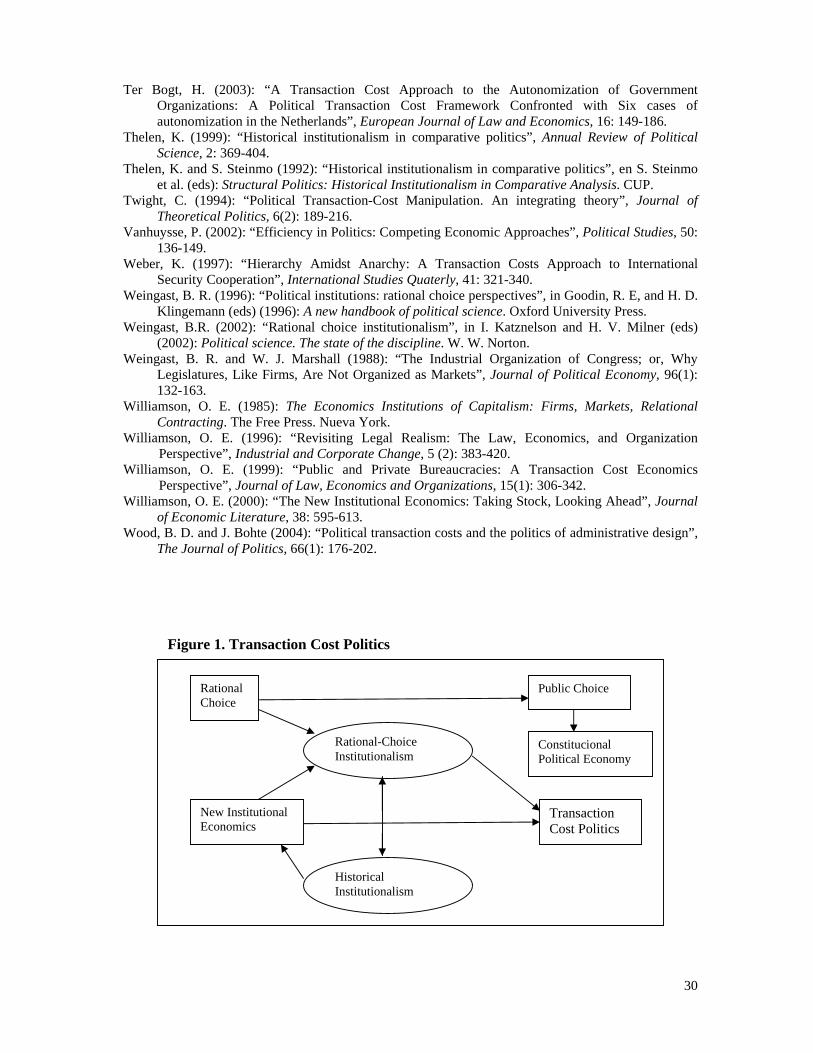
30

Ter Bogt, H. (2003): “A Transaction Cost Approach to the Autonomization of Government Organizations: A Political Transaction Cost Framework Confronted with Six cases of autonomization in the Netherlands”, European Journal of Law and Economics, 16: 149-186.

Thelen, K. (1999): “Historical institutionalism in comparative politics”, Annual Review of Political Science, 2: 369-404.

Thelen, K. and S. Steinmo (1992): “Historical institutionalism in comparative politics”, en S. Steinmo et al. (eds): Structural Politics: Historical Institutionalism in Comparative Analysis. CUP.

Twight, C. (1994): “Political Transaction-Cost Manipulation. An integrating theory”, Journal of Theoretical Politics, 6(2): 189-216.

Vanhuysse, P. (2002): “Efficiency in Politics: Competing Economic Approaches”, Political Studies, 50: 136-149.

Weber, K. (1997): “Hierarchy Amidst Anarchy: A Transaction Costs Approach to International Security Cooperation”, International Studies Quaterly, 41: 321-340.

Weingast, B. R. (1996): “Political institutions: rational choice perspectives”, in Goodin, R. E, and H. D. Klingemann (eds) (1996): A new handbook of political science. Oxford University Press.

Weingast, B.R. (2002): “Rational choice institutionalism”, in I. Katznelson and H. V. Milner (eds) (2002): Political science. The state of the discipline. W. W. Norton.

Weingast, B. R. and W. J. Marshall (1988): “The Industrial Organization of Congress; or, Why Legislatures, Like Firms, Are Not Organized as Markets”, Journal of Political Economy, 96(1): 132-163.

Williamson, O. E. (1985): The Economics Institutions of Capitalism: Firms, Markets, Relational Contracting. The Free Press. Nueva York.

Williamson, O. E. (1996): “Revisiting Legal Realism: The Law, Economics, and Organization Perspective”, Industrial and Corporate Change, 5 (2): 383-420.

Williamson, O. E. (1999): “Public and Private Bureaucracies: A Transaction Cost Economics Perspective”, Journal of Law, Economics and Organizations, 15(1): 306-342.

Williamson, O. E. (2000): “The New Institutional Economics: Taking Stock, Looking Ahead”, Journal of Economic Literature, 38: 595-613.

Wood, B. D. and J. Bohte (2004): “Political transaction costs and the politics of administrative design”, The Journal of Politics, 66(1): 176-202.

Figure 1. Transaction Cost Politics

Rational-Choice Institutionalism

Rational Choice

Public Choice

New Institutional Economics

Transaction Cost Politics

Historical Institutionalism

Constitucional Political Economy

Political Transitions in Ancient Greece andMedieval Italy: An Analytic Narrative

Leandro De Magalhães�

University of Bristol

August 23, 2012

Keywords:Political Transitions; Wars; Ancient Greece; Athens; Venice;Genoa; Democracy; Republic.

1 Introduction

Models of political transitions to democracy or on the extension of the

su¤rage have tended to focus on the 19th and 20th centuries (Acemoglu

and Robinson (2001), Lizzeri and Persico (2004), and LLavador and Oxoby

(2005)), and on disputes over redistribution or over the provision of economic

public goods such as infrastructure. These issues are relevant for the period

intended in these papers but as we go back in history, the de�ning public

good is defence and the contention policy issues seem to be whether to go to

war and which wars to �ght.

DeMagalhaes and Giovannoni (2012) propose a model where wars play

a key role in explaining political transitions. They model the bargaining

game that may bring an absolutist ruler to hand over power to an assembly

of citizens (the commercial elites in the paper). Wars determine both the

policy available to the players (whether to go to war and which wars to

�ght) and their threat points (what happens to the players when a war is

�e-mail:leandro.magalhaes@bristol.ac.uk

1

lost). In DeMagalhaes and Giovannoni (2012) the focus is on the English

case and the Glorious Revolution of 1688. The objective of this paper is to

provide an analytic narrative to test whether the model in DeMagalhaes and

Giovannoni (2012) is relevant to the understanding of political transitions in

Ancient Athens, Medieval Venice, and Genoa.1

The literature on the historical emergence of inclusive institutions has

focused on the economic changes that made it easier for rule by parliament

to emerge. Bates and Lien (1985), for example, formalizes the idea that the

tax elasticity of a sector increases its bargaining power. They show that the

most elastic sector will be taxed less and that the equilibrium policy will

be closest to the preferred policy position of the most elastic sector. As the

economy becomes more dependent on trade and manufacture and less on

agriculture we should observe a transfer of power to the commercial classes.

A similar argument is made in Levy (1988), where stable institutions must

include a form of quasi-voluntary �nancial contribution to the state. Fleck

and Hanssen (2006) focus on ancient Greece to show that the extension of

political powers may be necessary to provide the right economic incentives

when e¤ort is not observable.

In DeMagalhaes and Giovannoni (2012) the rise of commercial wealth is

also one of the key parameters of the model and a necessary condition for the

transition to rule by parliament to occur. The key di¤erence is that Bates

and Lien (1985), Levy (1988), and Fleck and Hanssen (2006) describe how

a particular economic environment makes it easier for a transition to occur.

As we will see below their broad predictions of the joint rise of commercial

wealth and of democracy (or rule by parliament) holds true for both ancient

Greece and Medieval Italy, but to understand the transitions themselves we

need to look at the role of war.

A large literature has focused on how the threat of war drove the forma-

tion of the state and helped states build capacity (see Tilly (1990), Ho¤man

1For a detail description of the method of analytic narrative see Arias (2012).

2

and Rosenthal (2000), Besley and Persson (2009), Gennaioli and Voth (2011),

Boix et al. (2011), and Arias (2012)). In these papers a war is a common

threat and the defence of the country is a common-interest public good. The

objective of these papers is to explain institutional changes such as the size

of the states, investments in �nancial capacity, on a judicial system, or on a

centralizing bureaucracy. The institutional change we are interested in here

is a transition to rule by assembly and considerable constraints on the exec-

utive (we will call such a regime a democracy or rule by assembly, council,

or parliament).

The model in DeMagalhaes and Giovannoni (2012) builds on Acemoglu

and Robinson (2001), where the handing-over of power is a commitment

device to ensure higher redistribution for the poor in the future. High re-

distribution is necessary to prevent the poor from acting on their threat of

revolution. Contrary to Acemoglu and Robinson (2001), DeMagalhaes and

Giovannoni (2012) focus on wars. The ruler will be unable to commit to

going to the wars preferred by the commercial elites in the future. Hand-

ing over power to an assembly (where the commercial elite plays the leading

role) solves this commitment problem and buys the �nancial assistance of

the commercial elites during a defensive war, when the ruler is at risk.

Wars are introduced in DeMagalhaes and Giovannoni (2012) by building

on Jackson and Morelli (2007), where wars have di¤erent risk-reward ratios

for rulers and citizens. DeMagalhaes and Giovannoni (2012) allow for di¤er-

ent types of war. Some wars, called misaligned, have an intrinsic bias: the

ruler receives an ego-rent from winning it, but they brings little economic

return to both the ruler and to the commercial elites. Alternatively, aligned

wars are also available: both the commercial elites and the ruler receive high

economic returns if an aligned war is won, but there are no ego-rents involved.

A key example of misaligned wars are costly dynastic wars that bene�t the

ruler and his kin but not the commercial elites. Examples of aligned wars are

commercial wars that expand the markets for the commercial elites�products.

3

DeMagalhaes and Giovannoni (2012) show that for an absolutist ruler to

hand over power to an assembly, there must be a credible threat that the

sitting ruler will be replaced if the war is lost. The commercial elites must

prefer the alternative invading ruler to their sitting ruler. This condition is

satis�ed, for example, if the invading ruler is better at winning wars (maybe

because of his alliances with other foreign powers). The commercial elites

may then prefer to withhold �nancial assistance to the sitting ruler on a

defensive war against the stronger contender. If they do so, they increase

the probability of a transition to either rule under the stronger contender,

or to their self rule as the sitting ruler may be willing to hand-over power in

return for their assistance. Therefore, one of the predictions of our model is

that transitions should occur in countries of intermediate military strength

(if they were hegemonic there would be no credible threat to the ruler).

DeMagalhaes and Giovannoni (2012) also show that transitions to rule by

parliament are likely to be preceded by a period of unstable absolutist rule,

which is characterized by a ruler who goes on dynastic wars and defensive

wars without the assistance of the commercial elites.

We will also confront the evidence in ancient Greece and medieval Italy

with Ticchi and Vindigni (2009), where the threat of war helps the elite make

a credible commitment - in the form of democratization - to the citizen-

soldiers, who demand redistribution in return for exerting e¤ort during wars.

As we will see their model seems particularly relevant for the �rst steps of

representative government in Greece, where the army and later the navy was

manned by the citizens. For Venice and Genoa this also played a role, but

the main constraint seems to have been the �nancing of the �eet.

In summary, we will go through historical examples of transitions to rule

by assembly and check what was the role, if any, played by wars. Did the

transitions take place during a period of strong foreign threat? Is there

evidence that the aristocracy and the merchants had diverging opinions on

foreign policy; that the merchants withheld resources from their ruler; that

4

the merchants preferred a foreign ruler to the sitting ruler? By trying to

answer these questions we should be able to gauge the relevance of the model

in DeMagalhaes and Giovannoni (2012) in helping us understand the political

transitions in ancient Greece and medieval Italy.

2 Political transitions in ancient Greece

Before looking into the political reforms of Athens in detail, let�s brie�y

discuss the evidence from general trends towards democratic government in

ancient Greece. There seems to be a clear link between economic activity, in

particular trade, and democracy. This evidence supports the predictions of

models such as Bates and Lien (1985), Levy (1988), and DeMagalhaes and

Giovannoni (2012).

Speci�c to ancient Greece, Fleck and Hanssen (2006) show how democracy

can mitigate a time inconsistency problem. Workers and property owners

must put unobservable e¤ort to plant and maintain olive trees in the Athenian

hills that only bear fruits years later. The time inconsistency problem arises

because the aristocracy can not commit ex ante not to expropriate the fruits

of the laborers� investment. The hand-over of power to the producers is a

way to mitigate this problem. Democracy is therefore more likely to arise

the greater are the gains from solving this time inconsistency problem.

The Athenian example contrasts with Sparta according to Fleck and

Hanssen (2006). Sparta�s vast plains were ideal for growing grain. Not only

is the e¤ort exerted by the workers in grain production more easily observ-

able but also the time inconsistency is of a smaller scale. There was little

economic gain for the Spartan elite in handing over power to grain producers.

Fleck and Hanssen (2006) extend their analysis to other cities and �nd

support for their model. Cities with dry soil unsuitable for grains such as

Argos achieved moderate democracy whereas cities with richer soils such as

Corinth and Thebes were oligarchies.

5

In DeMagalhaes and Giovannoni (2012) one of the key variables is the rel-

ative importance of commercial wealth (versus land). Raa�aub and Wallace

(2007) (pg. 43) discuss how there is evidence that some archaic cities - in the

period before 480 - had democratic constitutions. These are: Achaea (coast

of mainland Greece), Croton (Sicily), Acragas (Sicily), Ambracia (coast of

mainland Greece), Argos (next to coast on mainland Greece), Chios (coastal

island facing Izmir), Cyrene (coast of Lybia), Heraclea Pontica (coast of

Turkey), Megara (coast near Athens), Naxos (Greek island), and Syracuse

(Sicily). It is interesting to note that all these are coastal cities and o¤-shots

from Greece. They would have invariably been highly dependent on trade.

The other important consideration is that a form of government with

some degree of representativeness appeared even in Sparta, away from the

coast and surrounded by high quality soil for grain production. Neither the

models of Fleck and Hanssen (2006) or DeMagalhaes and Giovannoni (2012)

explain these institutional changes. These changes are better understood

in the context of the model of Ticchi and Vindigni (2009), where power is

granted to the citizen-soldiers in order to guarantee their e¤ort during war.

The advances in warfare practice that led to Hoplite regiments manned

by small landowners (those who could a¤ord the weapons and the time o¤

from their farms) created some sense of equality in Sparta and in the rest

of Greece (see Raa�aub and Wallace (2007) pg. 37). In Sparta this took

the form of the set of laws called the Great Rhetra, laid down sometime in

the 9th century. It established the two hereditary Kings of Sparta, a council

of 28 elders, and that a full assembly should have �nal decision on state

matters. It also divided the population into villages and tribes, which made

military organization into phalanxes easier. Eventually, the two kings gave

themselves veto power �if the assembly spoke crookedly�.2 Besides this veto

power, the militarization of all aspects of life, potentially also voting, suggests

2See Raa�aub and Wallace (2007) pg. 39 for more details and primary sources.

6

that Sparta was not a fully �edged Democracy.3

Within the interpretation of DeMagalhaes and Giovannoni (2012) the

lack of democratic institutions in Sparta could be due not only to the lack of

trade, but also to Sparta becoming hegemonic - at least on land. There seems

to have been few credible threats to the rule of the Spartan elite. Without

such a threat there was no incentive for the elite to hand over power.

2.1 Athens

The transition to Democracy in Athens has, by most accounts, consisted of

three steps: Solon�s reforms in 594, Kleisthene�s reforms in 508, and Ephialte-

Perikles�reforms in 462-450.

2.1.1 Solon - 594

The main innovation of Solon�s reform in 594 was to change how status

had been de�ned in Athenian society (and therefore a place in public life).

Status was no longer determined by belonging to a hereditary aristocracy

but was linked instead to wealth, which was measured by the amount of

agricultural output and on the capacity to either keep a horse, a span of

oxen, or neither.4 Solon�s reforms also included an assembly of 400 (100

from each of the four Ionic tribes) with limited powers. Participation in the

Assembly was probably restricted to the top land-owning classes, as were the

o¢ ces of the nine Archons (the executive o¢ ces). Solon also codi�ed civil

and criminal law.

The reforms of Solon unlike the later reforms do not seem directly moti-

vated by a foreign threat, but are described as the results of socio-economic

strife within Athens. Osborne (2009)(pg. 211) describes Solon�s world as �a

world of bitter con�ict between the elite�. Moreover, Osborne (2009) (pg.

213) goes on to describe how the economy of Athens was changing rapidly

3See Raa�aub and Wallace (2007) pg. 344See Hansen (1991) pg. 30. for further details and primary sources.

7

during that time. Athenian �ne pottery and amphorae (used to transport

olive oil and wine) had been found all over the Mediterranean from around

700BC onwards. According to Osborne (2009) this new trade related wealth

generated competition within the elite and possibly between the elite and

the poor as trade created an incentive to maximize agricultural production.

The interpretation of Solon�s institutional reforms seem closely related to the

political-economy model proposed by Fleck and Hanssen (2006).

2.1.2 Kleisthene - 508

Kleisthenes�s reforms in 508 extended the assembly to 500, reorganized the

four old Ionic tribes in Attica (the region surrounding Athens) into 10 new

tribes and, most importantly, extended political rights to those who could

a¤ord to be part of a hoplite regiment (each of the 10 tribes had to supply one

regiment). Political right was also extended to all the demes (villages) of At-

tica and was no longer con�ned to Athens itself. Kleisthene also introduced

the law of ostracism, which allowed Athenians to vote for important political

�gures to leave the city for a certain period of time without losing title or

property.5 In 501 a board of 10 generals was introduced. These generals

commanded the army jointly with the polemarch (one of the nine Archons).6

The generals were elected by popular vote and the post could be held re-

peatedly - contrary to most other public o¢ ces. The generals yielded great

in�uence over Athenian policy. Both Themistocle and Cimon held the post

of polemarch within the nine Archons in the early 5th century and Perikles

was elected general repeatedly later in the 5th century.

The reforms of Kleisthene were directly linked to foreign threats and both

the model in DeMagalhaes and Giovannoni (2012) and Ticchi and Vindigni

(2009) help us understand this transition.

Athens was under the rule of the tyrant Peisistratos and his son Hip-

5See Hansen (1991) pg. 35. for further details and primary sources.6See Hansen (1991) pg, 34/35 for more details and primary sources.

8

pias from 561 until 510. Sparta attacked Athens in 511 and lost to Hippias

(who made use of Thessalian mercenary support to defend Athens). Sparta

attacked again and was able to capture Hippias�children; in exchange for

the hostages Hippias went to exile in Sigeion.7 Osborne (2009) suggests that

Sparta�s motives were part of a deliberate policy to increases its in�uence be-

yond the Peloponnese. The wealth and size of Athens would be an important

addition to Sparta�s network of allies against Argos (a rival city-state).8 In

the past Sparta had generated allies by delivering cities from their unpopular

tyrants.9

With the tyrant Hippias in exile Athenian factions fought for power. Is-

agoras, who favored an alliance with Sparta, was elected as archon. Kleis-

thenes, who was defeated tried to gather popular support by proposing the

political reforms described above. Sparta invaded Athens again to support

Isagoras and forcing Kleisthenes into exile. The Athenian people rioted and

were able to defeat Isagoras and the Spartan forces. Kleisthenes� reforms

were subsequently implemented.10

Kleisthenes� reforms had important military consequences. The newly

formed Assembly of the 500 gave a clear say in foreign policy to the hoplite

classes all over Attica. This new power was immediately put into use with

Kleisthenes himself ostracized for supporting an alliance with Persia.11 The

organization of Attica in 10 tribes and 139 demes strengthened and mod-

ernized the Athenian army, their dependence on mercenaries was reduced.12

The power of the people over foreign a¤airs would increase even further with

7See Osborne (2009)(pg. 277) for more details and primary sources. See also Hansen(1991) pg. 36.

8See Osborne (2009)(pg. 275).9Athenian stories about the fall of Hippias either omit Spartan intervention or mention

that the intervention was due to the oracle of Delphi, see Osborne (2009)(pg. 277) formore details and primary sources.10see Osborne (2009)(pg. 278) for more details and primary sources. See also Ober

(2007).11See Fornara and Samons (1991) pg. 56 for more details and primary sources.12See Osborne (2009)(pg. 279)

9

the creation of an elected board of generals starting in the year 501.

Kleisthene�s reforms handed over power from the elites to the Athenians

citizens who were needed to both �nance and man the hoplites regiments.

It�s noteworthy that the tyrants were not able to summon the Athenian

themselves to �ght against Sparta, but had to rely on mercenaries to defend

their rule. The Spartan attack on Athens can be interpreted, in the context of

DeMagalhaes and Giovannoni (2012), as a defensive war where the Athenians

(the commercial elites in the model) chose not to help defend their ruler;

instead, their aim was to trigger a political transition, which eventually took

place.

The Athenian army had parallels with the mass armies of the early 20th

century, as citizen-soldiers must exert unobservable e¤ort in war. In Ticchi

and Vindigni (2009) external threats make possible an equilibrium where

the elites hand over power (which guarantees redistribution) and the citizens

exert e¤ort during a war. So this is another way to understand the extension

of political rights in the late 6th century.

The threat to Athens remained high, not only were the Persians intent on

conquering Greece, but the exiled tyrant Hippias seemed to be in alliance with

the Persians.13 The new Athenian army defeated the Persians at Marathon

in 490. The threat persisted as Aigina (a prosperous island rivaling Athens

in commerce)14 sided with Persia. Themistocles as archon persuaded the

Assembly to pay for the harbor of Peiraieus to be forti�ed and later to use

the revenue of a recent silver strike to pay for 100 triremes to be added to

the Athenian navy. In 480 Athens led the victory in a naval battle against

Persia at Salamis. In 478 the Dealian league was created solidifying Athenian

naval supremacy in the Aegean.15 This turn to the sea is important to

understand the further developments of the Athenian democratic reforms.

It�s also important to notice that the decision to invest the silver windfall on

13See Hansen (1991) for more details and primary sources.14See Osborne (2009) pg. 308.15See Hansen (1991) pg. 36.

10

the navy was approved by the assembly, the alternative would have been to

pay each Athenian a lump sum transfer. The investment on the navy was a

deliberate move to strength Athenian naval power and a deliberate choice of

foreign policy.

The political consequences of this turn to the sea were clear as 100

trimeres implied organizing almost 20,000 men to row them.16 Most of these

men would have to come from the property-less class, the thetes. Both models

DeMagalhaes and Giovannoni (2012) and in particular Ticchi and Vindigni

(2009) would predict that political powers would be extended to the thetes

and that is what eventually happened under Ephialtes and Perikles.

2.1.3 Ephialte - 462

In 461/2 Ephialtes proposed a reform to transfer power from the Areopagos

- the main judiciary body and a bastion of the land owning aristocracy - to

other institutions more representative of the Demos (mostly the Assembly).

Opposers of these reforms included the aristocracy and Cimon, an archon

and general of the Athenian navy. The reform was passed while Cimon

was away with a large hoplite contingent to help Sparta suppress a helot

revolt. The conditions under which the reform was approved shows that a

dispute over foreign policy was a key issue: those that proposed the political

reforms were also against the willingness of Cimon to assist the Spartans. The

other key element is that due to a large regiment of hoplites being away, the

assembly was tilted towards the poorest citizens.17 The reforms resulted in

bitter dispute with Cimon ostracized as he tried to reverse the reforms and

Ephialtes eventually assassinated. Raa�aub (2007)(pg.122) explains these

democratizing reforms and the support for a prominent Athenian naval role

as a result of the empowerment of the thetes, who were essential for the navy

and who therefore bene�ted directly from Empire. Perikles�reforms followed

16See Osborne (2009) pg. 310.17See Raa�aub (2007) pg. 113 for details and primary sources.

11

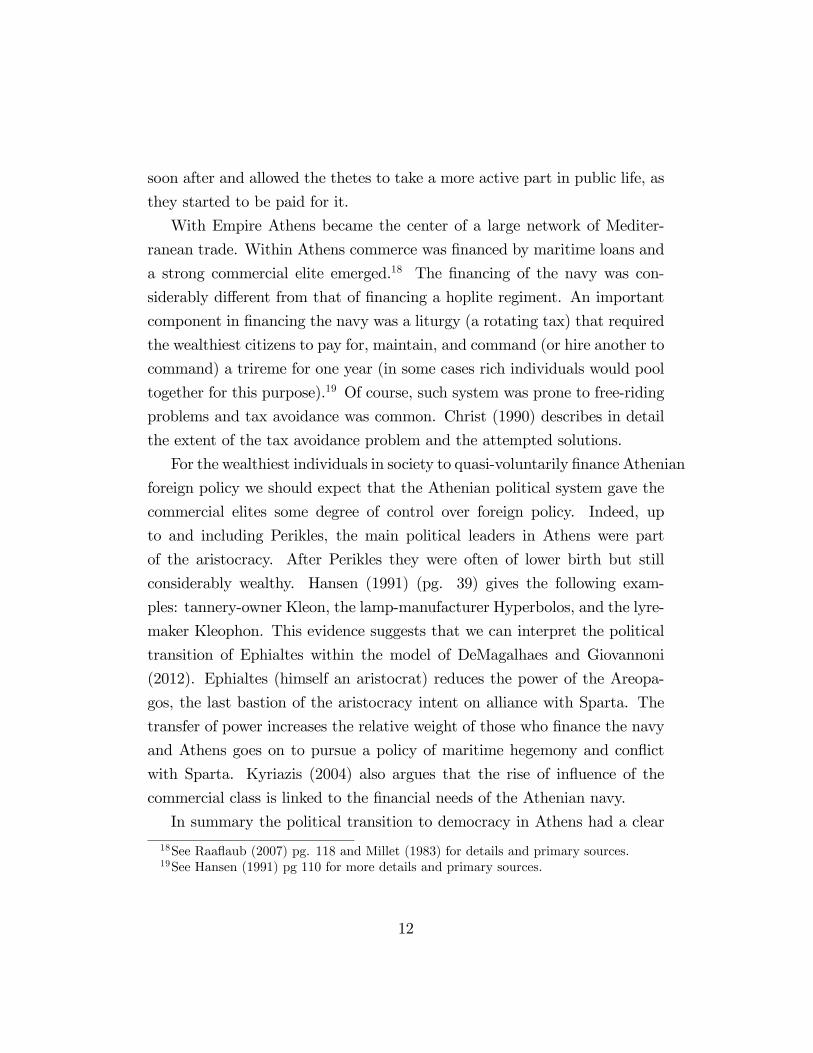
soon after and allowed the thetes to take a more active part in public life, as

they started to be paid for it.

With Empire Athens became the center of a large network of Mediter-

ranean trade. Within Athens commerce was �nanced by maritime loans and

a strong commercial elite emerged.18 The �nancing of the navy was con-

siderably di¤erent from that of �nancing a hoplite regiment. An important

component in �nancing the navy was a liturgy (a rotating tax) that required

the wealthiest citizens to pay for, maintain, and command (or hire another to

command) a trireme for one year (in some cases rich individuals would pool

together for this purpose).19 Of course, such system was prone to free-riding

problems and tax avoidance was common. Christ (1990) describes in detail

the extent of the tax avoidance problem and the attempted solutions.

For the wealthiest individuals in society to quasi-voluntarily �nance Athenian

foreign policy we should expect that the Athenian political system gave the

commercial elites some degree of control over foreign policy. Indeed, up

to and including Perikles, the main political leaders in Athens were part

of the aristocracy. After Perikles they were often of lower birth but still

considerably wealthy. Hansen (1991) (pg. 39) gives the following exam-

ples: tannery-owner Kleon, the lamp-manufacturer Hyperbolos, and the lyre-

maker Kleophon. This evidence suggests that we can interpret the political

transition of Ephialtes within the model of DeMagalhaes and Giovannoni

(2012). Ephialtes (himself an aristocrat) reduces the power of the Areopa-

gos, the last bastion of the aristocracy intent on alliance with Sparta. The

transfer of power increases the relative weight of those who �nance the navy

and Athens goes on to pursue a policy of maritime hegemony and con�ict

with Sparta. Kyriazis (2004) also argues that the rise of in�uence of the

commercial class is linked to the �nancial needs of the Athenian navy.

In summary the political transition to democracy in Athens had a clear

18See Raa�aub (2007) pg. 118 and Millet (1983) for details and primary sources.19See Hansen (1991) pg 110 for more details and primary sources.

12

element of creating the incentives for individuals to participate and put e¤ort

in war as described in Ticchi and Vindigni (2009). However, as the Athenian

navy becomes the main military instrument and Athens�wealth starts to

depend more and more on commerce, the model of DeMagalhaes and Gio-

vannoni (2012) seems more appropriate to understand the consolidation of

Athenian democracy and its stability until the Macedonian conquest. The

commercial elites were indespensable to �nance Athenian defences, and were

able under constant foreign threats (Persia and Sparta) to gain power and

yield it to try and further their commercial interests.

3 Political transitions in medieval Venice and

Genoa

3.1 Venice

There are two important dates in the Venetian transition from elected monar-

chy (with some degree of heredity) to a Republican system with considerable

checks and balances on the executive: 1032 and 1172. The events around 1032

illustrate how the dodgeship came close to becoming a hereditary monarchy,

but there were no clear institutional changes in 1032. The key political reform

took place 1172, when the dodge was constrained to abide by the decisions

of his council.

Venice began its history under control of the Byzantine Empire. The

�rst rulers in the area were Byzantine o¢ cials appointed by the Emperor

in Constantinople (see both Lane (1973) and Norwich (1983)). By the 8th

century Venice was electing their ruler in a general assembly (the concio or

Arengo), most likely dominated by the powerful families.

With time powerful dodges were able to raise their sons to rule together

with their father, setting them for succession. With the Orsoleo family Venice

came close to becoming a hereditary monarchy. Pietro Orsoleo II was a very

13

successful ruler and was able to marry his older son to the niece of the Byzan-

tine Emperors. His eldest was raised to rule with him and set for succession.

With the premature death of his older son in 1005, Pietro raised his third

son Otto to the dodgeship and retired. Otto was made a dodge at 16 and

married the daughter of King Stephen of Hungary. In 1017 Otto placed two

brothers in the two most important religious positions in Venice: as Patriarch

of Grado and as Bishop of Torcello. Due to further contentious religious and

political appointments he was ousted and sent to exile in Constantinople in

1024. King Stephen swiftly attacked and conquered Venetians cities along

the Adriatic. The Byzantine Emperor withdrew trading privileges granted to

Venice that formed the backbone of Venetian wealth.20 With such external

pressure the interim dodge Centranico abdicated and Otto was called back,

but died before his return to Venice. An obscure member of the Orseolo

family tried to seize the dodgeship but was ousted.21

The �rst important reform in Venice came as a response to this attempt

by the Orseolo family to establish hereditary rule in Venice. The Vene-

tians chose as their next dodge Domenico Flabanico in 1032, a wealthy silk-

merchant with no link to the old powerful families of Venice. According Nor-

wich (1983) there was no clear reforms in Venetian law then, which already

called for elections and described the positions of councillors as a counter-

balance to the dodge. There was a change in what was acceptable behavior

for a ruler - specially regarding nepotism. By choosing a dodge with no dy-

nastic pretensions the Venetians were sending a clear signal that they did

not favor a hereditary monarchy. From 1032 onwards Norwich (1983) notes

that no father passed the dodgeship to his son. The executive power of the

dodgeship, however, remained intact and the dodge continued to rule as an

elected monarch.

Even with this aversion to a hereditary monarchy, by 1172 Lane (1973)

20For a description of the self enforcing institutions that promoted trade in Venice inthis period see Gonzáles de Lara (2011).21For more details see Norwich (1983), chapter 5.

14

remarks that the dodgeship was held by members of the Michiel family for

sixty-two out of the last seventy-six years. The change in the law that would

consolidate the constraints on the executive came in 1172 and would be linked

to external threats and to the �nancing of the Venetian navy.

Norwich (1983) (chapter 8) describes how in 1171 relations between Byzamtium

and Venice were at the point of break-down. The Emperor blamed the Vene-

tians for an attack on the Genoese at Galata (the Genoese settlement oppo-

site Constantinople) and had all Venetian citizens and property con�scated

in Constantinople and other ports of the Empire.

Dodge Vitale II Michiel led the war preparation under strenuous �nancial

conditions - Norwich (1983) (chapter 8) mentions that all the revenues of the

state for at least a decade had already been pledged for previous debts. Dodge

Vitale ordered a forced loan; every citizens with means had to contribute; and

all able men were expected to man the navy. With the �eet already at sea the

Byzantine Emperor asked for a Venetian embassy to go to Constantinople

and work out a peace plan. Dodge Vitale accepted what turned out to be a

ploy of the Emperor to gain time. During the wait the plague spread in the

�eet, and when Vitale received the bad news from the ambassadors he was

forced to return to Venice in humilation have not only lost men and ships

(that had to be burnt) to the plague but also bringing the plague to the city.

He was ousted and murdered in the streets.

Before immediately electing a new dodge the Venetians decided to impose

political reforms. They were now at war with both the eastern and western

Roman Empires, in dire straits �nancially, and had a navy in di¢ culties.

The institutions that followed were designed to constraint the power of the

dodge, whose unconstrained power was blamed for the position Venice found

herself in. A Great Council of 480 was to be nominated by the di¤erent

neighborhoods of Venice, they were to hold o¢ ce for one year and nomi-

nate the chief o¢ cials of the state, including the dodge (which until then

was o¢ cially elected by the Arengo, which comprised all citizens of Venice).

15

Instead of nominating the dodge directly the Great Council nominated 11

electors who then chose the dodge and presented their choice to the people

as a done deal (see Norwich (1983) chapter 9 for details and Lane (1973) pg.

95-101). The other reform was to increase the number of councillors from

two to six, the councillors were also given more power to restrain the dodge.

The Senate gained more power specially in foreign a¤airs. Norwich (1983)

sees the e¤ect of these reforms as to �weaken both the apex and the base of

the administrative pyramid while strengthening its center�.

The choice of the next dodge clearly re�ected a change in power towards

the �nanciers of the Republic. Dodge Sebastiano Ziani was one of the wealth-

iest men in Venice. According to Norwich (1983) (chapter 9) Ziani suspended

payment on the new government bonds (from the forced loans to �nance the

navy). It seems there was little resentment, which demonstrates a willingness

of the creditors (Venetians themselves) to �nance the state under the new

dodge. Venice also immediately sued for peace with Byzantium, who refused

to accept the terms, so that the consolidation of the new regime was done

under considerable foreign threat and at a point where Venice was militarily

weakened.

The political reform in Venice 1172 can be best understood in the light

of the model in DeMagalhaes and Giovannoni (2012). These reforms seem

designed to transfers power to the �nanciers of the state, the wealthy mer-

chants, and away for the old quasi-nobility and the populace. During a period

of high external threat and dire �nancial straights, the power over foreign

policy was entrenched in the hands of those who could a¤ord to �nance the

defence of the state. Once in power they would decide over foreign policy

with their interests in mind, and not with the objective of setting up a hered-

itary monarchy or of antagonizing foreign powers that were essential for the

wealth of the state.

16

3.2 Genoa

Genoa has no clear historically accepted date for a transition to rule by coun-

cil or parliament. The best candidates are the rise of Gugliemo Boccanegra

as Captain of the People in 1257 and later of Simone Boccanegra as the �rst

Dodge of Genoa in 1339. In the interval Genoa was also ruled by podestas,

foreign rulers, and the aristocracy. Neither form of government proved stable.

Genoa is well known for the internal strife that would regularly escalate

into civil war between di¤erent noble families (clans) throughout its history.

Since power never consolidated with any of the key clans, by 1190 the families

agreed (under the in�uence of the Holy Roman Emperor) to be ruled by a

Podesta, a foreigner who would rule Genoa with a mandate of one year.22

Besides the con�ict between di¤erent noble families, there was also a

con�ict between the noble families and the people, in particular what Epstein

(1996) (pg. 206) called the popolo grasso, the rich merchants who were not

part of the nobility. Epstein (1996) (pg. 137) describes the events on 1257.

After a crash in the economy a popular revolt elected Gugliemo Boccanegra

as Captain of the People and a new council of thirty-two anziani. The new

regime�s policies were geared towards �the people who put him in o¢ ce,

the middling traders and master artisans, not the poor or the traditional

elite�(Epstein (1996) pg. 138). Interestingly one of the �nancial reforms of

Boccanegra was aimed at preventing the default on state debt and led to

the creation of a �precautions markets for public securities� to �nance the

Genoese state (pg. 147). Gugliemo Boccanegra was to stay in o¢ ce for �ve

years before he fell (probably due to a coup by some of the nobles).

In 1339 after a period under foreign rule by Robert Anjou, King of Naples,

and a period of unstable rule by the old nobility, the people revolted and cre-

ated a new position of Dodge electing Simone Boccanegra (grandnephew of

22See Epstein (1996)(pg. 88) for more details and Greif (2006) for a game theoreticanalysis of the podestaria.

17

Gugliemo).23 Again this was the rule of the merchant classes and not of the

nobles. Epstein (1996) (pg. 205) notes that we have details for 16 of the 22

ducal councillors; none is a noble and there are �two drapers, three butch-

ers, a shield maker, and a master of the wool guild�of those that identi�ed

themselves by profession. The new governor strengthened Genoese defences

and again had to consolidate public debt without repudiating any old debt.

By 1340 a new �eet was out to Pera for commercial ventures. Epstein (1996)

(pg. 207) notes that these policies re�ected a �turning away from civil war

to the more congenial task of making money�. Simone Boccanegra was also

to fall by 1344 under the imminent attack of an alliance made up of nobles

who had been excluded from power.24

Another characteristic of Genoa was that it was repeatedly ruled by for-

eigners. Not because they were conquered but by choice. The podesta is the

key example but also Henry VII in 1311, the King of Naples (1331-1335),

and later submitting to France and then to Milan.

The events in Genoa highlight two important aspects of the model in

DeMagalhaes and Giovannoni (2012). One is the clear con�ict between the

nobility�s dynastic concerns and attempt to impose aristocratic rule, versus

the merchant classes interests in a stable government with stable �nances

and following commercial objectives abroad. DeMagalhaes and Giovannoni

(2012) model this con�ict with the choice of a misaligned (dynastic) war

versus an aligned (commercial) war. The second aspect is the will of the

merchant classes to support foreign rule. A necessary condition for politi-

cal transitions in DeMagalhaes and Giovannoni (2012) is a credible outside

threat, someone ready to replace the current monarch (or aristocratic fam-

ilies in the case of Genoa). For the threat to be credible it must be that

the commercial elites prefer a foreigner to their sitting ruler. Repeatedly in

Genoa this seems to have been the case.23See Epstein (1996) pg. 204.24See Epstein (1996) pg. 208.

18

Why was there no stable transition to rule by assembly in Genoa? Within

the logic of DeMagalhaes and Giovannoni (2012) there seems to have no

clear moment where the country faced a hostile foreign threat and �nancial

di¢ culties (as Venice did in 1172). Another is to recognize a shortcoming

of the model in DeMagalhaes and Giovannoni (2012) where the aristocracy

is modeled as a single ruler. It seems clear that a divided aristocracy with

competing dynastic objectives played a key role in preventing a stable form

of government from appearing in Genoa.

4 Final Remarks

A picture emerges of di¤erent driving forces for political transitions. One

driving force is the creation of representative institutions as a response to

economic conditions: either in order to help solve a time inconsistency prob-

lem in the economy - olive oil production in Athens, and international trade

in Athens, Venice, and Genoa - or due to a relative growth in importance

of the economic sectors with high tax elasticity. The papers of Bates and

Lien (1985), Levy (1988), Fleck and Hanssen (2006), and DeMagalhaes and

Giovannoni (2012) predict that representative governments are more likely to

arise where trade �ourished. The evidence seems to support this prediction.

The cities in the ancient and medieval world that developed representative

institutions with considerable constraints on the executive were the leading

trading cities of those times. Moreover, they seem to have had little choice

but to turn to the sea. As Fleck and Hanssen (2006) notes, ancient city-

states like Athens had insu¢ cient and inadequate soil for grain production;

this was also true for Venice and Genoa.

Political transition may also come as a solution to a problem of how to

motivate an army manned by the state�s own citizens. This motive seems

to have been key for the creation of the Great Rhetra in Sparta, and also

for the political inclusion of the hoplites and later of the landless class (the

19

thetes) in Athens. Similar forces must have played a role in how the populace

was given a voice to chose their dodges both in Venice and later in Genoa.

The model that best helps us understand these driving forces is Ticchi and

Vindigni (2009).

A transition may also come about as a established aristocratic elite chooses

to hand over power to the people, or to the commercial elites, so that the

state can raise enough funds to defend itself against a foreign threat. This

seems a plausible interpretation of the events in Athens where members of the

aristocracy (Kleisthenes, Ephialtes, and Perikles) were the ones to propose

the institutional reforms discussed above. In Venice the powerful families

proposed the institutional changes of 1172 and in both key moments (1032

and 1172) chose dodges who were wealthy merchants of lower birth. The

model that best explains this aspect of political transition is DeMagalhaes

and Giovannoni (2012).

We also found evidence to support two aspects of political transitions

that are speci�c to the model of DeMagalhaes and Giovannoni (2012). The

�rst is that a transitions to rule by parliament should be preceded by an

unstable period where the ruler goes to wars without the support of the

citizens or the merchants. The tyrant of Athens, Hippias, for example, had

to rely on mercenaries to defend the city against Sparta. Later, Cimon�s

assistance to Sparta in containing a helot revolt was a contentious foreign

policy move and was opposed by Ephialtes and his supporters. In Venice

The Dodge Vitale II Michiel followed policies that put in jeopardy Venice�s

key commercial interests in both the Byzantine and western empires. The

dodge had to eventually resort to forced loans in order to fund the navy

against Byzantium.

The second aspect is that the model in DeMagalhaes and Giovannoni

(2012) predicts that we should observe political transitions only in states of

intermediate military strength. This is so because there must be a credible

external threat. Athens faced clear threats from both Persia and Sparta (to

20

whom it would eventually lose the Peloponnesian war). Venice was under

direct threat from both Byzantium and from the western Roman Empire

when the power of the dodge was constrained in 1172.

Finally, Genoa provided an example that showed the limitations of the

model in DeMagalhaes and Giovannoni (2012). An important aspect of the

Genoese political system was internal strife between di¤erent clans with dy-

nastic interests. Genoese leaders never consolidated power as the tyrants of

Athens or the dodges of Venice were able to do. This could suggest that the

centralization of power (as described in Tilly (1990), Ho¤man and Rosenthal

(2000), Besley and Persson (2009), Gennaioli and Voth (2011), and Arias

(2012) ) may be an important and counter-intuitive step towards constrain-

ing the executive through rule by parliament. Centralized power may have

to be established before it can be handed-over.

21

ReferencesAcemoglu, D. and Robinson, J. A. (2001). A Theory of Political Transitions.

The American Economic Review, 91(4):938�963.

Arias, L. M. (2012). Building Fiscal Capacity in Colonial Mexico:

From Fragmentation to Centralization. Working Paper - Juan March

Institute - Madrid.

Bates, R. H. and Lien, D. (1985). A Note on Taxation, Development and

Representative Government. Social Science Working Paper 567 - Caltech.

Besley, T. and Persson, T. (2009). The Origins of State Capacity: Property

Rights, Taxation, and Politics. The American Economic Review,

99(4):1218�1244.

Boix, C., Codenotti, B., and Giovanni, R. (2011). Political Economy of

Institutions, Democracy and Voting, chapter War, Wealth and the

Formation of States, pages 45�74. Springer-Verlag.

Christ, M. R. (1990). Liturgy Avoidance and Antidosis in Classical Athens.

Transactions of the American Philological Association, 120:147�169.

De Magalhaes, L. and Giovannoni, F. (2012). War Financing and the

Transition from Absolutism to Rule by Parliament. Mimeo Bristol

University.

Epstein, S. A. (1996). Genoa and the Genoese, 958�1528. North Caroline

Press.

Fleck, R. K. and Hanssen, F. A. (2006). The origins of democracy: A

22

model with application to ancient greece. Journal of Law and Economics,

49(1):115�146.

Fornara, C. W. and Samons II, L. J. (1991). Athens from Cleisthnes to

Pericles. University of California Press.

Gennaioli, N. and Voth, H.-J. (2011). State Capacity and Military Con�ict.

Working Paper CREI-Barcelona.

Gonzáles de Lara, Y. (2011). Political Economy of Institutions, Democracy

and Voting, chapter Self-Enforcing, Public-Order Institutions for

Contract Enforcement: Litigation, Regulation, and Limited Government

in Venice, 1050-1350, pages 95�115. Springer-Verlag.

Greif, A. (2006). Institutions and the Path to the Modern Economy.

Cambridge University Press.

Hansen, M. H. (1991). The Athenian Democracy in the Age of Demosthenes:

Structure, Principles and Ideology. Blackwell.

Ho¤man, P. T. and Rosenthal, J.-L. (2000). Divided we fall: The Political

Economy of Warfare and Taxation. Caltech Working Paper.

Jackson, M. and Morelli, M. (2007). Political Bias and War. The American

Economic Review, 97(4):1353�1372.

Kyriaziz, N. C. and Zouboulakis, M. S. (2004). Democracy, Sea Power and

Institutional Change: An Economic Analysis of the Athenian Naval Law.

European Journal of Law and Economics, 17:117�132.

23

Lane, F. C. (1973). Venice A Maritime Republic. The Johns Hopkins

University Press.

Levy, M. (1988). Of Rule and Revenue. University of California Press.

Lizzeri, A. and Persico, N. (2004). Why Did the Elites Extend the Su¤rage?

Democracy and the Scope of Government, with an Application to Britain�s

�Age of Reform�. Quarterly Journal of Economics, 119(2):707�765.

Llavador, H. and Oxoby, R. J. (2005). Partisan Competition, Growth, and

the Franchise. Quarterly Journal of Economics, 120(3):1155�1189.

Millet, P. (1983). Trade in the Ancient Economy, chapter Maritime Loans

and the Structure of Credit in Fourth-century Athens, pages 36�52.

Chatoo&Windus - The Hogarth Press.

Norwich, J. J. (2003). A History of Venice. Penguin.

Ober, J. (2007). Origins of Democracy in Ancient Greece, chapter 4 �I

Besieged That Man�, pages 83�104. University of California Press.

Osborne, R. (2009). Greece in The Making 1200-479 BC. Routledge, 2

edition.

Raa�aub, K. A. (2007). Origins of Democracy in Ancient Greece, chapter 5

The Breakthrough of Demokratia in Mid-Fifth-Century Athens, pages

105�154. University of California Press.

Raa�aub, K. A. andWallace, R. W. (2007). Origins of Democracy in Ancient

Greece, chapter 2 �People�s Power�and Egalitarian Trends in Archaic

24

A Collective-Action Theory of Fiscal-Military State Building

Luz Marina Arias∗

September 27, 2012

“Where benefits are not earmarked, ‘somebody else should pay’ is always a powerful motivation

in tax policy.” Alt (1983, p. 194).

The emergence of the fiscal-military state in the eighteenth century granted the central gov-

ernment new and unprecedented roles. In England, fiscal collection was increasingly centralized

and put in the hands of a new and efficient fiscal bureaucracy, an army was created, and the navy

acquired world-renown reputation (O’Brien 1988 and Brewer 1989). Tax proceeds as a percentage

of national income rose from 3.5 percent in the 1670s to over 12 percent by the end of the eighteenth

century.1 Even though parallel attempts at fiscal modernization in Spain met with limited success

until the early nineteenth century, in colonial Mexico public officials succeeded at strengthening the

central administration with fiscal bureaucrats and a proficient accounting system. Mean growth

for the Mexico City Treasury averaged almost 60 percent in each of the decades between 1770 and

1800.2 Other European states followed in the late eighteenth and early nineteenth centuries.

Prior to this transition, most monarchs depended to a large extent on economic and local

elites for the collection of tax revenue and defense. Fiscal capacity was fragmented. The central

ruler invested minimally in monitoring and enforcement capacities to collect taxes. Treasuries and

∗I am grateful to an anonymous referee, David Baron, B. Douglas Bernheim, Paul David, Alberto Dıaz-Cayeros,Marc Dincecco, Rafael Dobado, Avner Greif, Luis Jauregui, Yadira Gonzalez de Lara, Steve Haber, Margaret Levi,Carlos Marichal, Romans Pancs, Alvin Rabushka, Gavin Wright, and the participants at the II International Confer-ence on Political Economy and Institutions in Baiona, the Social Science and History Workshop at Stanford University,and the Workshop on Endogenous Institutions and Political Conflict at UC Berkeley’s Center on Institutions andGovernance. This work would have not been possible without the financial support from the Stanford Institute forEconomic Policy Research, the John M. Olin Program in Law and Economics, Stanford Law School, and the Centeron Democracy, Development, and the Rule of Law (CDDRL) at Stanford University.

1O’Brien (1988), Table 2.2Klein (1985, 566-574).

1

fiscal institutions at the national level functioned primarily as recipients of the monies collected

by the local elites. Provincial authorities or economic actors organized in corporations—such as

aristocrats, merchants or ecclesiasts—were responsible for the collection and dispatch of taxes.

Rulers negotiated monetary transfers and loans with these elites and corporations, and granted

them exemptions and other privileges in return.3 For instance, in France the provincial Estates,

the assembly of the clergy, and tax farmers had tax authority and transferred funds to the Crown.4

The Spanish crown protected the merchant guild from foreign competition in the colonies, provided

them with defense in the form of convoys, and had a contract with them for the collection of the

alcabala (sales) tax in colonial Mexico.5

The fiscal-military state, then, implied losses of fiscal and other privileges for different elites.

Why did fiscally and politically powerful elites allow the ruler to increase fiscal centralization and

build-up militarily? To the extent that a ruler lacked the ability to unilaterally increase revenue

to provide an army or to strengthen fiscal administration, the compliance of at least a fraction of

the elites was necessary. Indeed, all across early modern Europe “provinces, estates, ecclesiastical

domains, privileged cities, and corporations, as well as noble families [...] and city states, maintained

privileges and defences against the imposition of more modern, centralized, universal, equitable,

and potentially more productive systems of taxation and finance.”6

Explanations for fiscal centralization emphasize the need to increase military establishments

as the major impetus for the growth of European states’ administrative apparatuses. There are

two approaches in the literature. One approach highlights the role of military conflicts.7 Military

conflicts facilitate fiscal reform because wars unify a diverse population (Huntington 1968; Herbst

2000; and Kiser and Kane 2001), or the benefits of taxation become more salient to citizens (Levi

1988; and Besley and Persson 2009) or capital investors (Mann 1988). Explanations in the second

approach underscore the need to constrain rulers upon granting them higher fiscal revenues. The

establishment of political institutions of representation, like a parliament, increases fiscal coopera-

tion by making commitments on public expenditures credible (North and Weingast 1989, Hoffman

3See, for instance, O’Brien (2011, 421-423), Brewer (1989), and Levi (1988).4Rosenthal (1998, 68).5Marichal (2007, 76-77) and Smith (1948).6O’Brien (2011, 432). See also Bonney (1999) and Storrs (2009).7See for instance Weber (1922), Skocpol (1979), Tilly (1990, 1993), Bonney (1995), and Brewer and Hellmuth

(1999). For a synthesis, see Campbell (1993) and O’Brien (2011).

2

and Norberg 1994; and Dincecco, Federico, and Vindigni 2011).8

Both of these approaches contribute to our understanding of the growth of the fiscal-military

state. Military conflicts provide a window for monarchs and governments to negotiate fiscal central-

ization by making salient the benefits of taxation. The second approach highlights, however, that

increases in the benefits of taxation may not translate in fiscal cooperation because of commitment

problems. A ruler with more fiscal and coercive powers may have incentives to expropriate elites

or renege on its debts.9 Some monarchs, however, succeeded at increasing fiscal centralization with

no institutions of representation in place. The evidence in Dincecco (2011, 27) shows that in many

European states fiscal centralization came before the formation of parliaments. Marichal (2007,

51) highlights that colonial Spanish America lacked representative assemblies yet Spanish officials

successfully implementated fiscal and military reforms in some regions in the eighteenth century.

In this chapter, I underscore the collective action problem present in fragmented fiscal regimes

that impeded the cooperation of the elites with the contribution of men and resources for the

defense of the territory. As such, the chapter emphasizes a commitment problem among the fiscally

powerful elites, rather than between the elites and the ruler, in the process of fiscal-military state

formation.10 In fragmented regimes, the ruler’s fiscal income rested on earmarking benefits to

elites. In the face of a threat of military conflict, fiscal fragmentation then led to a collective

action problem: each elite group had incentives to free ride on the contributions of others, thereby

contributing less than the socially optimal amount to military protection. The elites and the ruler

were stuck in a low-contribution and low-public-good-provision equilibrium. I argue that fiscal

centralization provided an institutional framework that allowed elites to commit to contribute to

military protection by ensuring others were contributing as well.11

That collective action problems are inherent to fiscally fragmented states has been well doc-

umented. Ertman (1999, 50) notes about the Estates in Germany that: “the structure of the

8A number of studies have expanded this argument and included qualifications. See for instance Stasavage (2002,2003), and Cox (2011). Ertman (1997) maintains that it is the timing of representative institution-building relativeto the onset of wars what explains the variation in fiscal capacity centralization.

9Further, in times of war, the ruler may discount the future more than other citizens (Levi 1988).10Many scholars have emphasized the role of collective action and free-rider problems in preventing the compliance

of actors with welfare-enhancing cooperation. See, for instance, Olson (1993), Greif (2006) and Greif, Milgrom, andWeingast (1994).

11Emerson (1983) provides a similar insight regarding state formation at an earlier stage in Baltistan. Greif (1998,2006) also highlights the importance of military threats and the need for elite cooperation in shaping the internalorganization of the state.

3

assemblies, divided as they were into separate curiae of elite groups each with their own distinct

privileges, tended to inhibit cooperation among the curiae and lead the nobility, clergy, and the

towns to focus on the defense of their narrow group rights.” Bates and Lien (1985, 57) quote from

Henneman (1971) that “fiscal jealousies led towns to make subsidy grants conditional upon similar

grants from other towns” in France. Summerhill (2008, 224-225) notes that because rulers bargained

separately with each group, fiscal fragmentation led to free riding and lower fiscal revenues.12

I provide a game-theoretic framework to analyze the conditions under which corporate and local

elites gain by surrendering to a central government their power to levy taxes.13 The analysis shows

that an increase in the probability of a threat of external invasion or internal unrest is more likely

to cause fiscal centralization when the elites are more dependent on the ruler for future economic

rents, and when the prospects of economic activity are higher. To the extent that the stakes from

military protection are aligned between the elites and the ruler, and the elites lack alternative ways

to commit to cooperate for defense, the elites acquiesce to fiscal capacity centralization.14

Historical evidence from the increases in fiscal centralization and military build up in seventeenth

century England and eighteenth century colonial Mexico provides support for the implications of

the theoretical argument. The evidence highlights the importance of the Civil War for England

and the Seven Years’ War for colonial Mexico, and the lack of standing armies in both regions, in

aligning the benefit from military protection between the elites and the ruler.

I present the formal argument in section 1. Section 2 confronts the theoretical argument with

evidence from English and colonial Mexican history. The final section concludes with a discussion

of the implications and further avenues for research.

12See also Levi (1988, 56-57).13This theoretical framework is built on the history of eighteenth-century colonial Mexico. Arias (2012) provides

a detailed historical analysis of the successful increase in fiscal centralization and military reorganization in colonialMexico after the Seven Years’ War.

14Besley and Persson (2009) and Besley and Persson (2011) study the joint development of fiscal capacity andmarket-supporting institutions. They also emphasize the salience of a public good for increases in fiscal capacity. Theiranalysis, however, does not incorporate the role of a powerful elite in blocking fiscal changes. In their comparativestudy of state finance in Britain and France, Hoffman and Rosenthal (1997) and Rosenthal (1998) illustrate theimportance of the difference in preferences for war between crown and elite when fiscal power is decentralized. Theydo not seek to explain transitions between fiscal regimes but only the impact of regimes on the number of wars fought.

4

1 FORMAL MODEL

This section provides a theoretical framework to explain why fiscal-military state building is more

likely when the probability of a threat of unrest or invasion increases. The focus is on the conditions

under which corporate and local elites have incentives to surrender their power to levy taxes to a

central government.

1.1 The Game

A central government, henceforth referred to as a ruler, R, interacts with n economic corporations,

indexed by i = 1, ..., n. These corporations are composed of agents that are able to make agreements

binding on all their members.15

The ruler is threatened with an invasion (or unrest) with probability θ. A public good (G)—

military defense—is necessary to defeat the invaders (or the unruly). In order to provide military

defense, the ruler depends on the contributions of the corporations because initially fiscal capacity

is fragmented. That is, the ruler depends on the corporations for the enforcement and collection of

fiscal monies. The corporations levy taxes and transfer some of the proceeds to the ruler.

The ruler is able to enforce bilateral contracts with the individual corporations, and by means

of these private contracts the corporations transfer part of their fiscal proceeds to the ruler. Each

bilateral contract is observed only by the parties to the contract. A contract with corporation i

specifies the amount xi ≥ 0 of good i that the ruler provides to corporation i in exchange for a

payment τi ≥ 0.16 Let (x, τ) = ((x1, τ1) , ..., (xn, τn)) be the profile of the ruler’s unilateral offers to

each corporation.

Under fragmented capacity, the corporations make contributions to the public good, gi ≥ 0,

that result in a level of the public good G = f(g), where g = (g1, ..., gn), f is (strictly) increasing in

g and fgigj > 0 for i 6= j. These contributions are voluntary because the ruler is unable to enforce

them under fragmented fiscal capacity.

15Historically, the corporations were represented by local authorities (e.g. majors) or heads of economic corporationsor guilds (e.g. aristocrats, merchants or ecclesiasts). Many scholars have stressed the importance of corporate formsin the development of tax systems. For instance, Strayer (1970), Henneman (1971), Prestwich (1972), Bates and Lien1985, and Levi (1988).

16Examples of publicly provided private goods include royal monopolies (e.g. exclusive access to trade betweenspecific regions), value added to commodities (e.g. mint silver coins), or the provision of local defense (convoys formerchants, fleets for miners). The collection of specific taxes by corporations also guaranteed loans between rulersand the lending corporations.

5

The ruler can propose to the corporations an increase in fiscal centralization, whereby the

corporations surrender to the ruler the power to levy taxes. The increase costs F to the ruler.

Under centralization, the ruler publicly announces and enforces uniform tax payments t ≥ 0 from

each i.

Timing

There are two periods. In the first period, all players observe θ. The ruler then chooses whether

to propose an increase in fiscal centralization or to keep fiscal capacity fragmented.17 If proposing

an increase in fiscal centralization, the ruler proposes a policy profile {t, x,G} consisting of tax

payments, a vector of private goods, and a level of the public good. If not proposing centralization,

the ruler proposes a “fragmented” policy profile {τ, x, g}, which includes a vector of payments,

private goods, and contributions to the public good. Each corporation accepts or rejects the policy

profile proposed by the ruler.

In the second period, if the ruler proposed an increase in fiscal centralization and at least n ≤ n

corporations accept, the ruler invests in a fiscal-military state and implements the policy agreed to

in the first period.18 If less than n corporations accept, fiscal capacity remains fragmented, the ruler

proposes a “fragmented” policy profile {τ, x, g}, and the corporations accept or reject the ruler’s

proposal. If the ruler did not propose an increase in fiscal centralization, the ruler implements the

“fragmented” policy profile agreed to in the first period.

Payoffs

A corporation’s payoff depends on the amounts of the private good, xi, and the public good, G,

and on (exogenous) overall economic activity, y. Some corporations benefit more from military

protection than others. A corporation is vulnerable to the threat (of an invasion or unrest) to the

17Historical evidence supports giving the ruler agenda-setting power. Monarchs and public officials typically playedan important role in coordinating economic elites and raising the elite’s awareness about the need to negotiate fiscal-military building.

18This framework does not explicitly incorporate the ruler’s commitment problem regarding t. Once a ruler investsin centralization, the ruler could renege on the agreement in period 1 and forcibly collect tax payments higher thanthose agreed to (see e.g. North and Weingast 1989). If fiscal capacity is fragmented, this commitment problem betweenthe corporations and the ruler is not an issue. Reputation ensures commitment from both corporations and rulerbecause exchanges under fragmented capacity rely on private contracts. A threat of reversion to fragmentation fromthe elite may not be credible, however, after the ruler has increased fiscal centralization. I discuss the commitmentproblem between ruler and corporations in the conclusion.

6

extent that the corporation depends on the survival of the ruler for future rents and protection.

Let αi ≥ 0 parametrize the degree to which corporation i benefits from the public good (G). A

higher αi implies greater dependence on the ruler and therefore a higher benefit from G.19 The

(expected) payoff of each corporation (when fiscal capacity is fragmented) is:

uFi (xi, G) = v(xi, y) + θαiy(f(gi, g−i), y),−gi − τi − ei.

where v and y are the values of the private and public goods, respectively, at a given level of

economic activity, θ is the probability of a threat, τi is corporation i’s payment to the ruler, and

ei > 0 is corporation i’s cost to collect taxes.20 The function v is increasing and concave in x

and y, vxiy > 0 for all i, and v(0, y) = 0. Accordingly, y is increasing and concave in G and y,

yGy > 0, and y(0, y) = 0. Recall that G = f(gi, g−i), where gi is corporation i’s contribution to

G. Each corporation’s payoff is a function of its individual exchange with the ruler if θ = 0. If,

by contrast, θ > 0, the corporation’s payoff is also a function of the public good. The more a

corporation depends on the ruler for economic rents (αi), the higher the benefit from the public

good.21 Finally, for any θ, an increase in economic activity increases the payoff of each corporation.

If corporation i rejects the ruler’s fragmented policy proposal, xi = 0 and corporation i receives

payoff u0 = v(0, y)+θαiy(f(0, g−i), y), where g−i denotes the contributions of all other corporations

given that corporation i is not contributing. There are positive externalities on those that do not

contribute to building an army because f is increasing in g−i for all i. That is, if θ > 0, all groups

with αi > 0 benefit and cannot be excluded from the military protection.22

When fiscal centralization is implemented, the (expected) payoff of each corporation is:

uCi (xi, G) = v(xi, y) + θαiy(G, y)− t,

where t is corporation i’s tax payment. (Recall the ruler sets ti = t for all i when centralizing tax

19For instance, some corporations may be able to keep their economic rents even in the case of a British takeoverof Spanish colonial territory, say, or they may have their own defense against internal uprisings.

20This cost captures the effort to assess, collect, enforce, and dispatch taxes locally.21The ruler and the corporations could also differ in their perception of the probability of a threat (θ). This can

be incorporated in the parameter αi.22This non-exclusion assumption distinguishes defensive warfare from predatory warfare. The former is a pure

public good, whereas the latter is a private good. The spoils of a war can be promised to only some groups, whileothers are excluded. For more on the distinction between defensive and predatory warfare see Emerson 1983.

7

collection.) Because the ruler collects and enforces taxes under fiscal centralization, ei = 0 for all i.

The ruler’s payoff is the revenue obtained from corporations’ payments. Let c(x,G) be the cost

of providing private and public goods in both fiscal regimes. Assume c is increasing and convex

in x and G, and cxixj = 0 and cxiG = 0 for all i. Then, the ruler’s payoffs under fragmented and

centralized fiscal capacities are, respectively:

uFR(x,G) =n∑

i=1

(τi + gi)− c(x,G),

uCR(x,G) = nt− c(x,G)− F.

1.2 Equilibrium

I solve for the pure-strategy subgame-perfect Nash equilibria (SPNE) of the game preferred by the

ruler.23 By backward induction, I first study the choice of payments and private and public goods

proposed by the ruler under fiscal fragmentation.

If fiscal capacity is fragmented, corporation i accepts policy profile {xi, τi, G} if and only if:

v(xi, y) + θαiy(f(gi, g−i), y)− gi − τi − ei ≥ θαiy(f(0, g−i), y). (1)

In the SPNE, the participation constraint in (1) binds for all i. Otherwise, the ruler would be able

to increase his payoff by increasing the payment for some corporations. By solving for τi from each

i’s binding participation constraint, we obtain the equilibrium payment τi for each corporation.

Substituting each τi in the ruler’s objective function, the ruler’s set of profit-maximizing policies is:

(x, G) ∈ arg maxx,g∈Rn

n∑i=1

v(xi, y) +n∑

i=1

θαi[y(f(gi, g−i), y)− y(f(0, g−i), y)]−n∑

i=1

ei − c(x,G). (2)

Solving we obtain the unique x and g the ruler proposes to the corporations under fragmented

fiscal capacity. Notice that the equilibrium amount of private goods is the same for all corporations

because the choice of x is independent from αi and g. The proposal x is also equal to the socially

23I assume the corporations accept the ruler’s proposal when indifferent. This allows me to rule out trivial equilibria.Also, the ruler makes a take-it-or-leave-it offer and so extracts all of the surplus from the corporations. Giving a highershare of the surplus to the corporations makes a transition to centralization more likely as long as the corporationsreceiving a large share of the surplus benefit from the public good (high αi).

8

optimal amount x∗ such that x∗ ∈ arg maxx∈Rn

∑ni=1 v(xi, y)− c(x,G).

Lemma 1. The equilibrium level of public good provision under fragmented fiscal capacity is lower

than the socially optimal: G < G∗.

Proof. The socially optimal level of public good provision solves:

G∗ ∈ arg maxg∈Rn

n∑i=1

θαiy(f(gi, g−i), y)− c(x,G). (3)

The first order conditions: θ∑

i αi∂y/∂G · ∂f/∂gi = ∂c/∂G · ∂f/∂gi for i = 1, ..., n, characterize

G∗. From (2), the first order conditions: θ∑

i αi∂y/∂G · ∂f/∂gi − θ∑

j 6=i αj∂y/∂G · ∂f/∂gi =

∂c/∂G ·∂f/∂gi for i = 1, ..., n, characterize G. The result follows because f is increasing in g. (The

solution is interior because of the assumptions on y and c.)

Under fragmented fiscal capacity, each corporation has incentives to transfer resources to the

ruler only to the extent that it receives xi. The corporations free ride on others in their contributions

to the public good, and the ruler has no means of enforcing these contributions. Internalizing the

lower contribution of each corporation, the ruler’s choice of G is lower than the socially optimal.

Lemma 1 allows us to define the social cost due to free riding as the increase in the aggregate

value from public good provision if the corporations were able to commit to pay: Y (G∗, y) −

Y (G, y) > 0, where Y (G, y) =∑n

i=1 y(G, y) = ny(G, y). If the groups were able to coordinate and

police themselves to commit to pay, there would be no cost from the free riding problem. The

difference Y (G∗, y)−Y (G, y) increases when the groups interact only with the ruler and are unable

to solve the collective action problem among themselves.

1.3 Investment in fiscal centralization

First, notice that when fiscal capacity is centralized the ruler maximizes fiscal transfers by choosing

the socially optimal amount G∗. Each corporation faces the following participation constraint when

the ruler proposes centralization:

v(xi, y) + θαiy(G, y)− t ≥ v(xi, y) + θαiy(f(g), y)− gi − τi − ei. (4)

9

The right hand side of (4) is constant and given by the equilibrium policy profile {τ , x, g}. The

corporations can refuse centralization and force the ruler to keep fiscal capacity fragmented. Sum-

ming over n and solving for t, we obtain nt ≤∑

i[v(xi, y) + θαiy(G, y)]−C, where C is a constant.

It follows that uCR(x,G) ≤∑

i[v(xi, y) + θαiy(G, y)]−C− c(x,G)−F . Therefore, the ruler sets the

maximum upper bound on net fiscal transfers by choosing G∗ as defined in (3).

Two conditions must hold for fiscal centralization to occur. First, the participation constraint

in (4) must hold for at least n corporations. The corporations can refuse centralization and the

ruler has no credible threat but to preserve fiscal fragmentation. Second, the ruler’s payoff must be

higher under centralization than under fragmentation. If the ruler’s payoff given the tax payment

necessary to obtain compliance from n corporations is less than the payoff from {τ , x, g}, the ruler

does not propose centralization.

Substituting in (4) for (τi, xi, g) and solving for t we obtain the maximum tax payment that

each corporation is willing to pay in exchange for the optimal level of the public good:

tMi ≤ v(xi, y) + θαi[y(G∗, y)− y(f(0, g−i), y)], for i = 1, ..., n. (5)

A couple remarks about this maximum tax payment are in order. First, the ruler obtains higher

maximum payments from those corporations who benefit more from the public good (αi). Second,

the ruler can obtain compliance from corporation i at a tax payment higher than the maximum

in (5) by compensating with private goods (a higher xi) or if the prospects of economic activity

increase.

I first obtain the SPNE assuming the ruler can collect corporation-specific tax payments and

provides the socially optimal amount of private goods x∗. The constraints in (5) bind for all i,

otherwise the ruler would be able to increase his payoff by increasing the tax payment for some

corporations. Let t∗i ≡ v(xi, y) + θαi[y(G∗, y) − y(f(0, g−i), y)] be the binding constraint in (5)

for i. The following proposition gives the condition under which policy profile {t∗, x∗, G∗} is an

equilibrium for n = n, where t∗ = (t∗1, ..., t∗n).

Proposition 1. At the SPNE, the ruler proposes policy profile {t∗, x∗, G∗}, all corporations accept

10

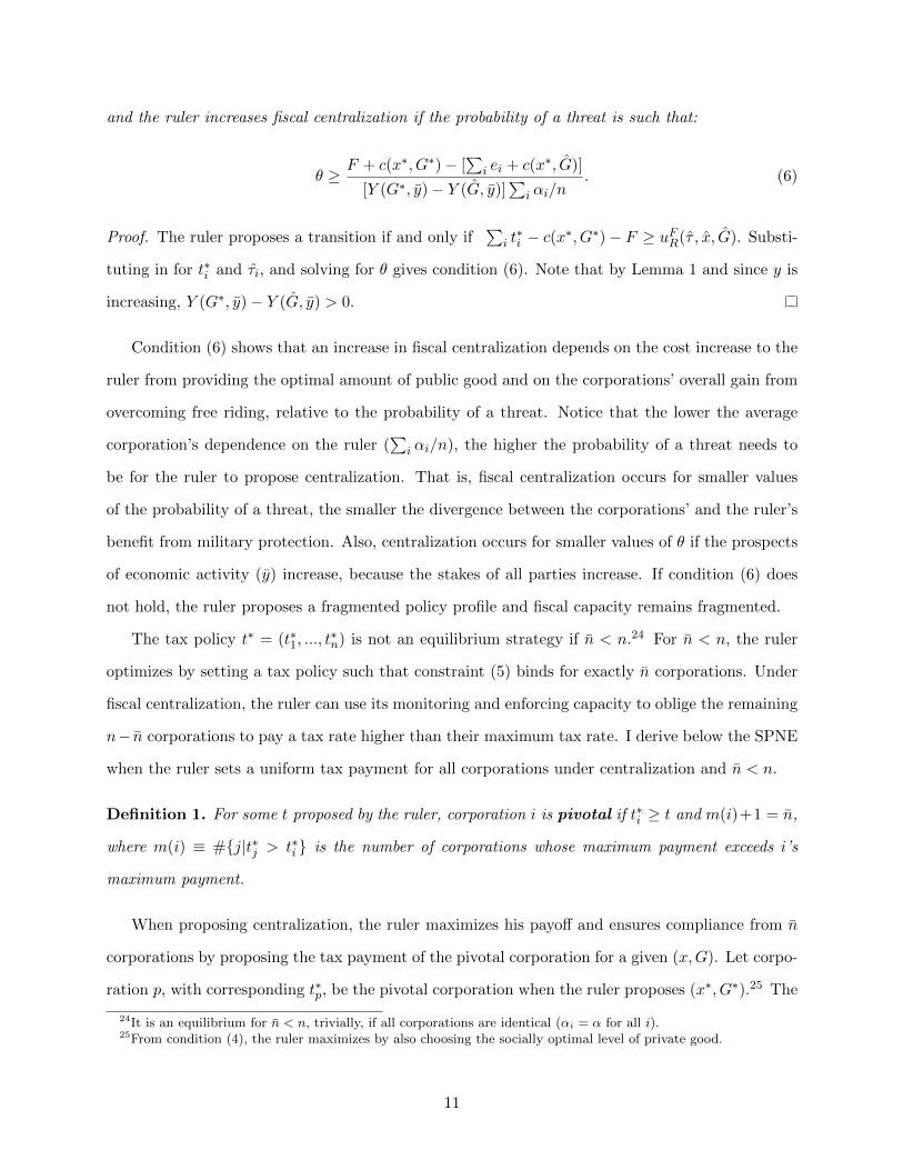
and the ruler increases fiscal centralization if the probability of a threat is such that:

θ ≥F + c(x∗, G∗)− [

∑i ei + c(x∗, G)]

[Y (G∗, y)− Y (G, y)]∑

i αi/n. (6)

Proof. The ruler proposes a transition if and only if∑

i t∗i − c(x∗, G∗)− F ≥ uFR(τ , x, G). Substi-

tuting in for t∗i and τi, and solving for θ gives condition (6). Note that by Lemma 1 and since y is

increasing, Y (G∗, y)− Y (G, y) > 0.

Condition (6) shows that an increase in fiscal centralization depends on the cost increase to the

ruler from providing the optimal amount of public good and on the corporations’ overall gain from

overcoming free riding, relative to the probability of a threat. Notice that the lower the average

corporation’s dependence on the ruler (∑

i αi/n), the higher the probability of a threat needs to

be for the ruler to propose centralization. That is, fiscal centralization occurs for smaller values

of the probability of a threat, the smaller the divergence between the corporations’ and the ruler’s

benefit from military protection. Also, centralization occurs for smaller values of θ if the prospects

of economic activity (y) increase, because the stakes of all parties increase. If condition (6) does

not hold, the ruler proposes a fragmented policy profile and fiscal capacity remains fragmented.

The tax policy t∗ = (t∗1, ..., t∗n) is not an equilibrium strategy if n < n.24 For n < n, the ruler

optimizes by setting a tax policy such that constraint (5) binds for exactly n corporations. Under

fiscal centralization, the ruler can use its monitoring and enforcing capacity to oblige the remaining

n− n corporations to pay a tax rate higher than their maximum tax rate. I derive below the SPNE

when the ruler sets a uniform tax payment for all corporations under centralization and n < n.

Definition 1. For some t proposed by the ruler, corporation i is pivotal if t∗i ≥ t and m(i)+1 = n,

where m(i) ≡ #{j|t∗j > t∗i } is the number of corporations whose maximum payment exceeds i’s

maximum payment.

When proposing centralization, the ruler maximizes his payoff and ensures compliance from n

corporations by proposing the tax payment of the pivotal corporation for a given (x,G). Let corpo-

ration p, with corresponding t∗p, be the pivotal corporation when the ruler proposes (x∗, G∗).25 The

24It is an equilibrium for n < n, trivially, if all corporations are identical (αi = α for all i).25From condition (4), the ruler maximizes by also choosing the socially optimal level of private good.

11

following result gives the condition under which the policy profile {t∗p, x∗, G∗} yields centralization

in equilibrium. I assume a corporation accepts if indifferent.

Proposition 2. At the SPNE, n corporations accept policy profile {t∗p, x∗, G∗} and the ruler invests

in a centralized fiscal administration if the probability of a threat of invasion or unrest is such that:

θ ≥F + c(x∗, G∗)− [

∑i ei + c(x∗, G)]

αpY (G∗, y)− Y (G, y)[∑

i αi/n]. (7)

Proof. The ruler proposes a transition if and only if nt∗p ≥ uFR(τ , x, G). Substituting in for t∗p and

τi, and solving for θ gives condition (7).

The gain from providing the optimal amount of military protection is now weighted by the

vulnerability to a threat of each corporation relative to that of the pivotal corporation. If the pivotal

corporation has a degree of vulnerability higher than the average, the transition to centralization

occurs for a lower probability of the threat than in Proposition 1, all else constant.26 However, if

the pivotal corporation has a lower benefit from the public good than the average corporation, the

condition in proposition 2 does not hold and the ruler does not propose centralization even though

it is socially optimal. This occurs because the ruler endures a loss in fiscal revenue from requesting

a uniform transfer rather than discriminating across corporations according to their benefit from

the public good.

1.4 Implications

Both propositions 1 and 2 highlight the main implication from the analysis. An increase in the

probability of a threat is more likely to cause an increase in fiscal centralization and military build-

up, the higher the corporations’ stakes on the survival of the ruler for their economic future. The

higher the corporations’ dependence on the ruler for future rents, the higher is the benefit from

the provision of the optimal military protection, and the more that the corporations are willing

to transfer under centralization. Also, all else equal, a higher level of economic activity facilitates

26This can be seen clearly by rewriting the denominator in condition (7) as follows and comparing it with thedenominator in condition (6):

αpY (G∗, y) − Y (G, y)∑i

αi

n= [Y (G∗, y) − Y (G, y)]

∑i

αi

n− Y (G∗, y)

∑i

αi − αp

n.

12

centralization by increasing the maximum a corporation is willing to pay under centralization and

by increasing the social gain from overcoming free riding. A fiscal regime may therefore remain

fragmented because the alignment between the benefits to the ruler and the corporate elites from

military protection is small, or the ruler’s cost of investing in centralization is too high.

Proposition 2 shows in addition that if the ruler is unable to collect corporation-specific pay-

ments (and is thus unable to extract all the corporations’ benefits from the public good), an increase

in fiscal centralization depends on the size of the ‘accepting’ coalition (n). In particular, we may

not observe centralization when it is socially optimal, if the pivotal corporation has a lower benefit

from the public good than the average corporation.

Finally, a couple remarks about the theoretical framework are in order. First, the analysis

emphasizes that unless the ruler has the support of some of the corporations, the increase in fiscal

centralization and military build up are not feasible. The corporations can refuse centralization and

the ruler has no credible threat except to preserve fiscal fragmentation. If, however, the ruler has

alternative or external sources of revenue to finance an army or impose centralization, negotiation

with the corporations may not play such an important role.

Second, the setup implicitly assumes the ruler has the authority and the ability to propose

and implement centralization. For the results to hold, the ruler must have legal authority and

the corporations must believe the ruler can credibly monitor and enforce tax collection. Lacking

a central actor with legal authority or the credible ability to monitor and sanction, an increase in

the probability of internal or external threat will not lead to an increase in fiscal centralization.

2 HISTORICAL EVIDENCE

To provide support for the theoretical argument, this section discusses historical evidence from the

transition to a fiscal-military state in seventeenth-century England and eighteenth-century colonial

Mexico.27 I organize the evidence around the two main factors highlighted by the theoretical

27Many scholars have documented the important changes in fiscal administration and enforcement, and in militarycapacity, that colonial Mexico and England underwent in the second half of the eighteenth century and the mid-seventeenth century, respectively. For colonial Mexico’s fiscal, administrative, and financial reforms, see for instanceFonseca and Urrutia (1791), Brading (1973, 1987), Elliott (1987), Klein (1998), Jauregui (1999), Coatsworth (1990),Knight (2002), Stein and Stein (2003), andMarichal (2007). Regarding colonial Mexico’s military reorganization,see McAlister (1953), Gutierrez-Santos (1961), Fisher (1982), Marichal and Souto Mantecon (1994), Kuethe (1986),Archer (1981, 1978) and Elliott (2006). The main sources for England are O’Brien (1988, 2011), Brewer (1989) andBrewer and Hellmuth (1999).

13

analysis leading to a fiscal-military reform: (1) military vulnerability and the alignment between

the corporate elites’ and the ruler’s benefit from military protection, and (2) the need for rulers to

negotiate with the corporate elites to obtain their compliance. Subsection 2.1 presents evidence for

England while subsection 2.2 discusses the evidence for colonial Mexico.

The cases of England and Mexico are pertinent because they allow us to isolate the public

good nature of military protection. When an army is created with predatory goals and the spoils

of war exclusively assigned to specific groups, military protection confounds both a private and

a public good nature. The objectives (at least initially) of the build up of a fiscal-military state

in seventeenth-century England and eighteenth-century Mexico were defensive. The historical ev-

idence below shows that they both lacked armies and had enjoyed relatively long periods of no

military involvement prior to the increase in the probability of a threat.

Also, the cases of England and colonial Mexico corroborate the importance of a ruler or central

government with the credible authority and ability to implement the fiscal-military reforms. Brewer

(1989) notes the importance of the British crown’s recognized authority and infrastructure in the

administration of justice for their success in building a fiscal-military state. In colonial Mexico,

the wars of independence (1810–1821) and resulting political instability provide an example of the

importance of legal authority. The internal and external threats faced by the elites in different

regions in the aftermath of independence from Spain did not lead to centralization. It took almost

fifty years for the region to stabilize its newly minted state. Centeno (2002) argues that this was a

result of the authority void left by the Spanish crown: no group was superior to the rest.

2.1 England

In contrast to other European nations, England lacked a standing army from the late fifteenth

to the late seventeenth centuries. Its landed aristocrats were also effectively demilitarized; by the

1640s “four out of five aristocrats had no military experience at all” (Brewer 1989, 12). This was

partly a result of England’s non-involvement with major international conflicts during that time-

period. According to Brewer (1989, 12), “England was sheltered not just by her insular position

but by the scale of war in early modern Europe.” The large increase in army sizes and number of

troops deployed made an invasion of England complicated, and an English invasion of the continent

difficult. English naval power only began to be established in the second half of the seventeenth

14

century. Castilian and French fleets managed to seize and sack various English ports during the

Hundred Years war. Further, prior to the seventeenth century, the navy depended heavily on

private support and armed merchantmen ships.28

The Civil War (1642–1651) marked a turning point for the need to secure the state against

domestic rivalries. An interregnum of civil warfare and challenges to hierarchy created the con-

ditions for a watershed in England’s fiscal and military history. Importantly, the succession of

events “forged a political consensus among England’s wealthy elites for an altogether stronger and

more centralized state, above all to maintain order and political stability, but also to afford greater

protection for the economy’s growing commercial interests overseas” (O’Brien 2011, 426). The

threat of internal political stability together with the lack of military protection provided the con-

ditions for an alignment of the executive’s and the elite’s benefit from creating a standing army

and strengthening the navy.

The important role played by Parliament in fiscal matters gives evidence of the need to negotiate

and obtain cooperation from the wealthy elites. Parliament decided on the selection of the levels

and types of taxes, the rules for their assessment and collection, and had control over the state

departments in charge of implementing those rules.29 In fact, the landed elites set the terms for

cooperation by initially avoiding direct taxes on land. It was not until 1799 that Pitt managed to

introduce Britain’s first income tax.30 “Only the armies of Revolutionary France and the probable

collapse of public credit prompted the political classes to accept [direct taxation]” (O’Brien 1988,

22).

English fiscal history shows the importance of a threat of internal unrest (evident after the

Civil war) in increasing fiscal centralization. By aligning the benefit from military protection for a

majority of the wealthy elites and monarch, a transition out of a low-contribution and low-public-

good-provision was possible. Also, the role played by parliament attests to the need to negotiate

with the elites and to the importance of centralized and public fiscal policies to ensure every elite

group that others were cooperating and contributing with the forging of a fiscal-military state.

28This paragraph summarizes Brewer (1989, 8-13).29Horowitz (1977) and O’Brien (2011).30O’Brien (1988).

15

2.2 Colonial Mexico

The Spanish crown faced practically no internal or external challenges in its American territories

during its first 200 years of colonial rule.31 The crown did not need to incur in major expenses

to defend its colonial territory and relied only on minimal forces at the ports and borders for the

protection of the Spanish American empire.32 The vulnerable position of the colonial Mexico is

evidenced by the efforts to garner a field army in 1762 in the port of Veracruz, on the coast of

the Gulf of Mexico.33 This port was the point of entry and exit for all European trade with New

Spain, and therefore one of the most guarded locations in colonial Mexico. In 1760, the port and

fortress were guarded by around 1,000 men.34 The port of Veracruz was vulnerable to attack just

before the end of the Seven Years’ War. The Viceroy Marques de Cruillas spent 3,398,471 pesos

of extraordinary funds to ready the fortifications and mobilize a force of 8,500 men in and around

Veracruz.35 This was a force eight times the size of the previous force. Notwithstanding, according

to the Viceroy, a much larger force was necessary to ensure the security of the kingdom.36

The lack of military protection in conjunction with the Seven Years’ War (1756–1763) identify a

watershed in colonial Mexican history. The Seven Years’ War changed the balance of power within

colonial territory among the European powers.37 In 1756, France declared war on Great Britain.

This was the beginning of the French-Indian War, as the conflict was known to the colonists. The

war was a struggle for primacy between Britain and France. For the first time in European history,

battles occurred in colonial territory.38 There were battles in India, North America, the Caribbean

isles, the Philippines, and coastal Africa, and Europe. By the autumn of 1760, all French territory in

mainland America was in British hands. An agreement made in August 1761 between the Bourbon

kings of Spain and France, the Family Compact, brought Spain into the war. In August of 1762,

31Arias (2012) provides a thorough historical analysis of colonial Mexico supporting the theoretical argumentpresented here.

32McAlister 1953, 2.33Colonial Mexico was part of one of the three viceroyalty in colonial Spanish America. After the conquest, the

Spanish divided the territory in two viceroyalties, New Spain and Peru, comprising roughly contemporary Mexico andPeru, respectively. Even though the viceregal government functioned as a link with the crown, many corporationsand powerful individuals negotiated directly with the government in Madrid.

34McAlister (1953, 2-3).35Archer (1981, 315).36McAlister (1953, 7).37See, for instance, Bonney (2004) and Elliott (2006).38Elliott (2006, 292). The conflict in North American soil began in 1754, two years before the formal outbreak of

war in Europe.

16

the British Royal Navy captures Havana, Cuba, and Manila in the Philippines. The war ended

following the Treaty of Paris on February 10, 1763, with a victory for Great Britain, who emerged

as the dominant European power.

The military defeats suffered by Spain during the Seven Years’ War marked a turning point

in the need to secure Spanish colonial possessions against British attack. Also, because of the

demographic recovery of the Indian population in the first half of the eighteenth century, many

provinces in colonial Mexico saw internal unrest increase to new levels.39 The Seven Years’ War,

together with the increased Indian unrest, marked the fiscal and military reorganization undertaken

by royal officials in the second half of the eighteenth century.

A growing body of scholarship demonstrates that reform was pursued through bargaining,

compromise, and political contestation between crown officials and the main elites and local au-

thorities.40 There were few military or police forces in the Spanish colonies that the crown could

rely upon for a top-down imposition, at least in the initial stages of reform. Furthermore, given

the condition of the imperial finances in Spain, it cannot be argued that the transition was paid

for with continental monies.41

The economic elites recognized the vulnerable position of the colonial empire in the locations

where the network of privilege and patronage that relied on the existence of the Spanish monarch

was most affected by the British threat. In the imperial capitals Mexico and Peru, and in Veracruz,

Cuba and coastal regions of Panama and Colombia the crown’s officials transformed the state

administration into a more highly structured apparatus, increased fiscal revenues by means of a

larger and more efficient fiscal bureaucracy, and renovated military establishments to a larger extent

than in other regions.42

Failed attempts to implement fiscal reform earlier in the colonial period also attest to the

importance of the Seven Years’ War. In 1626 the Count-Duke of Olivares attempted a fiscal reform

through the creation of the Union of Arms with the goal of sharing the burdens of defense in

mainland Europe among the different kingdoms in the Spanish peninsula and with the American

colonies. A fixed annual contribution was demanded from each and every part of the empire. The

39Fisher (1982, 219).40Kuethe and Inglis (1985, 122-123). See also Paquette (2007).41Net transfers are always positive from the Americas to Spain. See Irigoin and Grafe (2008), and Marichal and

Souto Mantecon (1994).42Marichal (2007, 48-80), Kuethe and Inglis (1985), Brading (1971), Brading (1987).

17

colonial corporations resisted the fiscal reforms and only temporary increases to trade tax rates

took effect.43

The evidence of negotiation with the elites, and earlier failed attempts to increase fiscal cen-

tralization, provide evidence for the inability to implement reform lacking an alignment between

the fate of the crown and that of the local and corporate elites regarding the provision of military

protection.

CONCLUSION

This chapter contributes to the literature by providing a complementary mechanism for why threats

of external invasion or internal unrest can lead to increases in fiscal centralization. Fragmented fiscal

capacity leads to free riding in the face of a threat. Fiscal centralization provides an institutional

framework that allows elites to commit to contribute to military protection by ensuring others also

contribute. The analysis shows that, even if there is agreement on the need to provide military

protection, it is not until a majority of the fiscally powerful have stakes on the survival of the ruler

for their economic future (and so their benefit from military protection aligns with that of the ruler)

that they can agree to the centralization of fiscal capacity.

The analysis here highlights two issues that suggest avenues for future research. First, the

theoretical argument assumes the ruler can commit to implement the policy profile agreed to

before the increase in centralization. Once a ruler invests in fiscal centralization, the ruler could

renege on the policy agreement and unilaterally increase future taxes or default on its debts.44

Reputation, however, limits the ruler’s incentives to renege on his agreements. If the future is

sufficiently important, the ruler has a reputation to maintain. Scholars have argued, however, that

in some cases reputation may not be enough to limit rulers, and that more elaborate institutional

arrangements may be required (e.g. institutions of representation).45

43Elliott (1986, 246-274). There was another failed attempt by the crown to centralize in the early 1700s.44Notice that fiscal fragmentation serves as a commitment devise for the ruler to pay its debts. By granting the

corporation/debtor the right to directly collect certain taxes, rulers were able to obtain payments in advance andguarantee the service of interest and repayment. The major legal form used for this transaction in Spain and itscolonies were the asientos. Asientos were contracts between the Crown and a private corporation or individualthrough which the latter promised to pay an amount to the Crown in exchange for the right to make use of therevenues resulting from a specific royal tax. See Dominguez Ortiz (1960), Conklin (1998), and Alvarez-Nogal andChamley (2011). For the case of England, see Brewer (1989, 93).

45See for example North and Weingast (1989), Greif et al. (1994), and Bullow and Rogoff (1989).

18

My analysis complements this literature on the need to constrain the ruler by emphasizing

another commitment problem—that between the elites resulting from free riding under fragmented

fiscal capacity. The results suggest that guaranteeing credibility from the ruler may not be enough.

If the benefit from overcoming free riding is not sufficiently large, both the ruler and the corporations

prefer fragmented capacity. The results also suggests that institutions of representation are not

necessary, at least in the initial stages of fiscal centralization, to the extent that the corporate elites’

and the ruler’s benefits from military protection are aligned in response to a threat. The case of

colonial Mexico corroborates that institutions of representation are not necessary for the elites to

agree to fiscal centralization. Future research needs to study more carefully the timing between

centralization and representation and the links between the two commitment problems mentioned.

Second, the theoretical argument does not incorporate dynamics to explain whether the in-

vestments in fiscal capacity are irreversible. Why should we not observe a reduction in fiscal

centralization once the threat disappears? Incorporating the complementarity between the cre-

ation of a standing army and a fiscal administration with monitoring and enforcement capabilities,

could make an increase in fiscal centralization difficult to reverse. In addition, the sunk-cost nature

of the investment in fiscal centralization can lead to irreversibility after the threat disappears, all

else constant. Historically, we do not typically observe transitions back to fragmented regimes once

a centralized administration with coercive enforcement is in place.

Both the theoretical argument and the evidence from England and colonial Mexico emphasize

the defensive, public-good aspect of military protection in leading to an increase in fiscal centraliza-

tion. In so doing, the analysis here may tell us something about the evolution of fiscal capacity at

other times and places. For a state relying on fragmented fiscal capacity to increase fiscal central-

ization, a sufficiently large shock jointly affecting the income of both the central government and

the relevant fiscal actors is necessary. Two conditions are key: that the shock creates a collective

action problem among the key actors, and that those actors believe the ruler can credibly monitor

and enforce tax collection. The new fiscal regime allows for the coordination of policies and the

enforcement of contributions.

19

References

Alt, J. E. (1983). The evolution of tax structures. Public Choice 41, 181–222.

Alvarez-Nogal, C. and C. Chamley (2011). Debt policy under constraints between Phillip II, the

Cortes and Genoese bankers. Working Papers in Economic History, Universidad Carlos III de

Madrid 11-06.

Archer, C. I. (1978). The Army in Bourbon Mexico, 1760-1810. Albuquerque, Univeristy of New

Mexico Press.

Archer, C. I. (1981). Bourbon finances and military policy in New Spain, 1759–1812. The Ameri-

cas 37 (3).

Arias, L. M. (2012). Building fiscal capacity in colonial mexico: From fragmentation to centraliza-

tion. Working Paper .

Bates, R. H. and D.-H. D. Lien (1985). A note on taxation, development, and representative

government. Politics and Society 14 (53).

Besley, T. and T. Persson (2009). The origins of state capacity: Property rights, taxation, and

politics. American Economic Review 99 (4), 1218–1244.

Besley, T. and T. Persson (2011). Pillars of Prosperity: The Political Economics of Development

Clusters. Princeton University Press.

Bonney, R. (Ed.) (1995). Economic Systems and State Finance. Clarendon Press.

Bonney, R. (Ed.) (1999). The rise of the fiscal state in Europe c. 1200-1800. Oxford University

Press.

Bonney, R. (2004). Towards the comparative fiscal history of Britain and France during the long

eighteenth century. In L. Prados (Ed.), Exceptionalism and Industrialization: Britain and Its

European Rivals, 1688–1815. Cambridge, U.K.: Cambridge University Press.

Brading, D. A. (1971). Miners and Merchants in Bourbon Mexico 1763-1810. Cambridge University

Press.

20

Brading, D. A. (1973). Government and elite in late colonial Mexico. The Hispanic American

Historical Review 53 (3), 389–414.

Brading, D. A. (1987). Bourbon Mexico and its American empire. In L. Bethell (Ed.), Colonial

Spanish America. Cambridge University Press.

Brewer, J. (1989). The Sinews of Power. London: Hutchinson.

Brewer, J. and E. Hellmuth (Eds.) (1999). Rethinking Leviathan: The Eighteenth Century State in

Britain and Germany. Oxford University Press.

Bullow, J. and K. Rogoff (1989). A constant recontracting model of sovereign debt. Journal of

Political Economy 97, 155–78.

Campbell, J. L. (1993). The state and fiscal sociology. Annual Review of Sociology 19.

Centeno, M. A. (2002). Blood and Debt: War and the Nation-State in Latin America. Pennsylvania

University Press.

Coatsworth, J. (1990). Los orıgenes del atraso. Mexico: Alianza Mexicana.

Conklin, J. (1998). The theory of sovereign debt and Spain under Philip II. Journal of Political

Economy 106 (3).

Cox, G. (2011). War, moral hazard, and ministerial responsibility. Journal of Economic His-

tory 71 (1), 133–61.

Dincecco, M. (2011). Political Transformations and Public Finances. Europe, 1650–1913. Cam-

bridge University Press.

Dincecco, M., G. Federico, and A. Vindigni (2011). Warfare, taxation, and political change: Evi-

dence from the Italian Risorgimento. Journal of Economic History 71 (4), 887–914.

Elliott, J. H. (1986). The Count-Duke of Olivares: The Statesman in an Age of Decline. Yale

University Press.

Elliott, J. H. (1987). Colonial Spanish America. In L. Bethell (Ed.), Spain and America before

1700. Cambridge University Press.

21

Elliott, J. H. (2006). Empires of the Atlantic World: Britain and Spain in America, 1492-1830.

Yale University Press.

Ertman, T. (1997). Birth of the Leviathan: Building States and Regimes in Medieval and Early

Modern Europe. Cambridge University Press.

Ertman, T. (1999). Variation in early modern state structure. In J. Brewer and E. Hellmuth (Eds.),

Rethinking Leviathan: The Eighteenth Century State in Britain and Germany. Oxford University

Press.

Fisher, J. (1982). Soldiers, society, and politics in Spanish America, 1750-1821. Latin American

Research Review 17 (1), 217–222.

Fonseca, F. and C. Urrutia (1791). Historia General de la Real Hacienda (1845-53 ed.). Mexico,

Impr. por V. G. Torres.

Greif, A. (1998). Self-enforcing political systems and economic growth: Late medieval Genoa.

In R. Bates, A. Greif, M. Levi, J. Rosenthal, and B. R. Weingast (Eds.), Analytic Narratives.

Princeton University Press.

Greif, A. (2006). Institutions and the Path to the Modern Economy: Lessons from Medieval Trade.

Cambridge University Press.

Greif, A., P. Milgrom, and B. R. Weingast (1994). Coordination, commitment, and enforcement:

The case of the merchant guild. The Journal of Political Economy 102 (4), 745–776.

Gutierrez-Santos, D. (1961). Historia Militar de Mexico, 1325-1810. Mexico, Ediciones Ateneo.

Henneman, J. B. (1971). Royal Taxation in Fourteenth Century France: The Development of War

Financing 1322–1356. Princeton University Press.

Herbst, J. (2000). States and Power in Africa: Comparative Lessons in Authority and Control.

Princeton University Press.

Hoffman, P. and K. Norberg (Eds.) (1994). Fiscal Crises, Liberty, and Representative Government

1450-1789. Stanford: Stanford University Press.

22

Hoffman, P. and J.-L. Rosenthal (1997). The political economy of warfare and taxation in early

modern Europe: Historical lessons for economic development. In J. N. Drobak and J. V. Nye

(Eds.), The Frontiers of the New Institutional Economics. San Diego: Academic Press.

Horowitz, H. (1977). Parliament, policy and politics in the reign of William III. Manchester.

Huntington, S. (1968). Political Order in Changing Societies. Yale University Press.

Irigoin, M. A. and R. Grafe (2008). Bargaining for absolutism: A Spanish path to nation-state and

empire building. Hispanic American Historical Review 88 (2).

Jauregui, L. (1999). La Real Hacienda de Nueva Espana. Su administracion en la epoca de los

intendentes: 1786–1821. Universidad Nacional Autonoma de Mexico.

Kiser, E. and J. Kane (2001). Revolution and state structure: The bureaucratization of tax admin-

istration in early modern England and France. American Journal of Sociology 107 (1), 183–223.

Klein, H. S. (1985). La economıa de la nueva espana, 1680–1809: un analisis a partir de las cajas

reales. Historia Mexicana 34 (4), 561–609.

Klein, H. S. (1998). The American finances of the Spanish empire: royal income and expenditures

in colonial Mexico, Peru, and Bolivia, 1680-1809. University of New Mexico Press.

Knight, A. (2002). Mexico: The Colonial Era. New York: Cambridge University Press.

Kuethe, A. J. (1986). Cuba, 1783-1815: Crown, Military and Society. University of Tennessee

Press.

Kuethe, A. J. and G. D. Inglis (1985). Absolutism and enlightened reform: Charles III, the

establishment of the alcabala, and commercial reorganization in Cuba. Past and Present 109,

118–143.

Levi, M. (1988). Of Rule and Revenue. Berkeley: University of California Press.

Mann, M. (1988). State and society, 1130–1815: An analysis of English state finances. In M. Mann

(Ed.), States, War, and Capitalism, pp. 73–123. NewYork: Basil Blackwei.

23

Marichal, C. (2007). Bankruptcy of Empire: Mexican Silver and the Wars between Spain, Britain

and France, 1760–1810. Cambridge University Press.

Marichal, C. and M. Souto Mantecon (1994). Silver and situados: New Spain and the financing of

the Spanish empire in the caribbean in the eighteenth century. The Hispanic American Historical

Review 74, 587–613.

McAlister, L. N. (1953). The reorganization of the army of New Spain, 1763-1766. Hispanic

American Historical Review 33 (1).

North, D. C. and B. R. Weingast (1989). Constitutions and commitment: The evolution of in-

stitutions governing public choice in seventeenth-century England. The Journal of Economic

History 34, 72–96.

O’Brien, P. K. (1988). The political economy of British taxation, 1660–1815. The Economic History

Review 41 (1), 1–32.

O’Brien, P. K. (2011). The nature and historical evolution of an exceptional fiscal state and its

possible significance for the precocious commercialization and industrialization of the British

economy from Cromwell to Nelson. The Economic History Review 64 (2), 408–446.

Olson, M. (1993). Dictatorship, democracy, and development. American Political Science Re-

view 87 (3).

Paquette, G. B. (2007). State-civil society cooperation and conflict in the Spanish empire: The

intellectual and political activities of the ultramarine Consulados and economic societies, c. 1780-

1810. Journal of Latin American Studies 39, 263–298.

Rosenthal, J.-L. (1998). The political economy of absolutism reconsidered. In R. Bates, A. Greif,

M. Levi, J. Rosenthal, and B. Weingast (Eds.), Analytic Narratives. Princeton University Press.

Skocpol, T. (1979). States and Social Revolutions. Cambridge: Cambridge University Press.

Smith, R. S. (1948). Sales taxes in new spain, 1575-1770. The Hispanic American Historical

Review 28 (2-37).

24

Stasavage, D. (2002). Credible commitment in early modern Europe: North and Weingast revisited.

Journal of Law, Economics, and Organization 18 (1), 155–186.

Stasavage, D. (2003). Public Debt and the Birth of the Democratic State: France and Great Britain,

1688–1789. Cambridge University Press.

Stein, S. J. and B. H. Stein (2003). Apogee of Empire. Spain and New Spain in the Age of Charles

III, 1759-1789. John Hopkins University Press.

Storrs, C. (Ed.) (2009). The fiscal-military state in eighteenth century Europe: essays in honour of

P.G.M. Dickson. Aldershot.

Strayer, J. R. (1970). On the Medieval Origins of the Modern State. Princeton University Press.

Summerhill, W. R. (2008). Fiscal bargains, political institutions, and economic performance. His-

panic American Historical Review 88 (2).

Tilly, C. (1990). Coercion Capital and European States, AD 990-1992. Cambridge, MA: Blackwell.

Tilly, C. (1993). European Revolutions. Oxford: Basic Blackwell.

Weber, M. (1922). Economy and Society (1968 ed.). New York: Bedminster.

25

Stable Constitutions in Political Transition∗

Katja Michalak†and Gerald Pech‡

August 29, 2012

∗We wish to thank Keith Schnakenberg and Norman Schofield for helpful comments.†Zeppelin University Friedrichshafen, email: katja.michalak@zu.de‡KIMEP University, Almaty, email: gp@geraldpech.net

1

1 Introduction

This paper develops a spatial model where an autocrat selects a status quoconstitution. This constitution may or may not be accepted by a succeedingelected constitutional assembly as a blue print for negotiations on constitu-tional reform. A constitution defines as legitimate a status quo point in policyspace with policy dimensions redistribution and social policy. Moreover, itguarantees property rights and provides a policy rule of how the status quopoint can be modified. We model constitutional design and reform as a dy-namic game. As the first mover, the autocrat is free in selecting the statusquo point. If accepted by the succeeding assembly, it becomes the defaultoutcome when the assembly enters negotiations over constitutional reformwhich take the form of changing the status quo policy. In the absence of aprior constitution or after a rejection of the prior constitution, the assemblyenters free negotiations on a new constitution.More recently, constitutional succession has become an issue in many

Arab countries where autocratic regimes were succeeded by freely electedgovernments. When the White House called for Husni Mubarak, then pres-ident of Egypt, to step down, the question immediately arose whether therules of succession would apply as laid out in the Egyptian constitution orwhether the constitution had to be suspended to negotiate a transition be-tween the old regime and the opposition (see Brown, 2011a). After Mubarakeventually resigned, the interim military government, i.e. the Supreme Coun-cil of the Armed Forces, adopted a provisional constitution which containedsignificant amendments and aimed at paving the way to parliamentary elec-tions.1 The elected parliament set out on what proved to be a bumpy roadtowards negotiations over a new constitution.Of these events, two facts stand out: On the one hand, the Mubarak

constitution turned out to be not acceptable to all parties involved in thetransition process. Therefore, on the face of it the Egyptian case is one ofdiscontinuity of the existing authoritarian constitution. On the other hand,the leadership of the military, which had significant bargaining power in thetransition process, was widely seen to be able to hold on to their privilegesand property interests2. These two observations suggest that the Egyptiantransition is an ambivalent case where the formal constitution handed downby the autocrat lacked perseverance yet the property order established underthe constitution was kept in place.Moreover, whilst this paper looks into the possibility for an autocratic

1For details of the process see Brown, N. (2011b)2Egypt’s Freedom, Financial Times, 20 May 2012

2

regime to select a constitution which is accepted as a blue print by its succes-sors, the Supreme Council of the Armed Forces faced a rather similar choiceproblem when drafting the amendments of the provisional constitution.3 Inprinciple, our framework should lend itself to analyzing constitutional choicein this slightly different context. Whilst it is still too early to judge theoutcome of this constitution project, at the time of finalizing this paper itappeared as if the army was revoking its support for the constitutional reformprocess in the face of a legislature dominated by Islamist parties.4

Chile, as the second example which we look at, is a clear example ofsuccessful constitutional succession.5 In 1980, the Chilean military juntaadopted a constitution which subsequently not only governed the internalworkings of the junta and imposed constraints on its exercise of power, butwhich set the rules by which the transition to democracy finally took place:In 1988, Pinochet stood for election, thereby sticking by the letter of theconstitution. Following electoral defeat, the Chilean parties of the right andthe center negotiated constitutional amendments which were adopted as partof a reformed constitution by plebiscite in 1989. The amendments includedrestrictions on presidential powers, the lowering of the quorum for changingnon vital parts of the constitution, admittance of parties of the left, and amodification of the relative voting power of civilians versus the military onthe national security council. In large parts, the constitution of 1980 remainsin place today.There are clear differences but also similarities between Egypt and Chile:

Chile has a long and recent history of constitutionalism. The Chilean con-stitution was a binding constraint on the dealings of the junta (see Barros,2002). Most significantly, transition took place because the regime, aftersome hesitation, obeyed the letter of the constitution. In Egypt, on theother hand, the transition of power was brought about by street protests.Common to both countries is the influence exercised by parties and organi-zations associated with the old regime during the transition period. In Egyptthis was mainly the military which served as a power broker during the rev-olution whilst in Chile these were the parties of the right which bargained inthe shadow of power which was projected by the military.In this paper, we see a preexisting constitution as a natural focal point

in the transition process which can serve both as a reference but also as a

3Other classification schemes agree on the ambiguity of the Egyptian case: In the frame-work of Munck and Leff (1997) the Egyptian transition can be classified as one of defeatof the old order. Yet if one considers the military as part of this order, one could equallyargue that the transition can be classified as a pact.

4Egypt Court Orders Parliament Dissolved, Financial Times, 15 June 2012.5For an overview see Barros (2002) and Montes and Vial (2005).

3

reversion point for constitutional reform. The reform process in which a soci-ety attempts to newly arrange its social compact creates many uncertainties.The negotiating parties may end up in a game of attrition where each triesto secure concessions from the other parties involved in the process. The at-tempt of constitutional reform may end in open conflict if the participationconstraint of one of the players is not satisfied. For those reasons, the electedsuccessor parties which are interested in changing the constitution may yetagree on the preexisting constitution as a default outcome in order to insureagainst the risks otherwise involved in negotiating a new constitution.If the autocrat expects a succeeding constitutional assembly to use a

preexisting constitution in that way, it creates an avenue through which theautocrat, in writing a constitution, can influence the power play after hisdemise. In this paper we assume that the interest group of the propertyowning class can exert sufficient influence on the autocrat to make him writea constitution on their behalf.We show, first of all, that constitutions exist which are stable in the tran-

sition process. Whether or not the autocrat strictly prefers to hand down aconstitution depends on who he expects to bargain over constitutional reform.If the autocrat expects that the future constitutional assembly is dominatedby parties which favor redistribution, he does not want to bind himself by theconstitution. If not a single party dominates the constitutional assembly andthe middle class opposes redistribution or it is expected to forge a coalitionwith the right dominate, stable constitutions exist which are in the interestof the autocrat. Here, our model provides a theoretical underpinning for thefrequently stated idea that a middle-class which is interested in maintainingproperty rights is a prerequisite for constitutional stability.6

Moreover, we show that if the autocrat can hand down a constitutionimmediately before his demise, he may choose to write a stationary consti-tution, i.e. a constitution which he predicts to be accepted by a succeedingconstitutional assembly without further amendment. Only if the autocratexpects that he will have to abide by the constitution himself for some time,he will compromise on the stationarity property. We also argue that, the-oretically, a succeeding assembly will elect the prior constitution as defaultbargaining outcome, irrespective of what it says. Hereby, cases are possiblewhere a preexisting constitution is accepted in the reform process even whenit has hardly constrained the autocrat and is significantly amended in thereform process.

6See e.g. Ordeshook (1997), Easterly (2001).

4

1.1 Related literature

Looking at the selection of rules in general and the constitution in particularin terms of manipulating strategic situations to achieve desirable outcomeswas advanced by Riker (1986) with his analysis of the events leading to theadoption of the American constitution.7 Our paper models constitutionalchoice in terms of the strategic selection of a status quo point in a spatialmodel. This places our model in a strand of literature which derives equilib-ria of the political game which are predicated on previous choices such as themove of an agenda setter or the selection of institutions. Tsebelis (2002), forexample, shows how institutions determine the set of veto players within aspatial policy framework and thus shape policy outcomes.8 Whilst constitu-tional norms typically provide general rules for policy selection rather thanmaking policy choices more directly, the selection of institutions togetherwith the legitimization of a status quo policy has implications for policyoutcomes. In the case of Chile and Egypt, one can argue that choices overpolitical institutions were often clearly aimed at preventing or promotingparticular policy outcomes.9

In our framework, a constitution provides a focal point which enablesagents to coordinate on Pareto-better outcomes compared to outcomes achievedin the absence of a constitution. A different way of understanding consti-tutions as coordination devices - understood as ”red-lines” the crossing ofwhich agents accept as triggers for coordinated action - has been introducedby Weingast (1997). Other approaches focus on the role of constitutions ascommitment devices by which a government can credibly pledge to upholdproperty rights (North and Weingast, 1989) or an autocrat to give legallyenshrined guarantees to his followers (Myerson, 2008). Moreover, Grossman(2002) gives conditions under which it is possible to design constitutions withself-enforcing properties - i.e. where agents abide by constitutional processes- when facing the alternative of descending into conflict. Pech (2009) andNaqvi, Neumärker and Pech (2011) focus on self-enforcing properties of con-

7See also Riker (1996). Schofield (2002) elaborates on this logic and applies it to theevolution of the American constitution.

8In a more general setting one may ask how the historical and/or constitutional choiceof rules determines the selection of rules which at later stages emerge from the politicalgame. See Barbera/Jackson, 2004 and Lagunoff, 2007.

9In the case of Chile, parties of the left were not admitted under the Pinochet constitu-tion but they were admitted under the reform constitution, provided they were not anti-system. The decision of the Supreme Council of the Armed Forces to dissolve a parliamentdominated by the Muslim brotherhood was a move which interfered with the institutionalset-up of post-revolutionary Egypt but was mainly aimed at preventing parliament fromselecting policies which were against the interests of the military rulers.

5

stitutions which contain the rule of law as a mechanism. Another strand ofliterature looks at constitutions in terms of the properties and desirabilityof the voting rules it provides.10 Finally, in an accompanying paper, Micha-lak and Pech (2012) provide a full equilibrium analysis which extends andapplies the present framework to the Chilean transition process. That pa-per, in more detail, focuses on the significance of middle class wealth forconstitutional stability.

1.2 Outline of the paper

Section 2 sets up the model. Section 2.1 presents negotiations in the absenceof a prior constitution or after its rejection. Section 2.2 details bargainingon constitutional reform in the presence of a prior constitution. Section 2.3derives optimal constitutions for the autocrat. Section 3 analyses the staticconstitutional choice problem of the autocrat. Section 4 extends our resultsto a dynamic setting. Section 5 discusses applications to different experiencesof political transition and derives conclusions from our framework.

2 The model

A constitution is a pair (t, x), representing a country’s basic choices11 onredistribution - associated with a tax rate t - and social policy x which maybe measured along a scale representing liberalism versus authoritarianism,secularism versus a greater role for religion in public life or the relative im-portance of the social solidarity principle versus the free market principle.12

The policy space = is T ×X = [0, 1]×<.There are three socio-economic groups, the clientele of the autocrat, R,

the middle class, M , and the working class, L. We do not explicitly modelthe military as a player. In the Chilean case the junta emerged from withinthe military. Therefore, one can identify the military in the aftermath oftransition as a lingering aspect of the junta and closely associate it withthe autocrat’s clientele. In Egypt, autocratic government and military wereorganizationally separate but the military leadership shared interests withthe possessing class and can, for the purposes of our model, be associated

10See, for example, Gersbach (2004) and Barbera Jackson (2006).11We do not discuss in this model rules governing post constitutional choices such as

electoral rules. Stability properties of electoral rules are discussed, for example, in Bar-bera/Jackson (2004).12Kitschelt (1996) finds that the majority of policy choices can be subsumed under a

distributional/communitarian dimension.

6

with the clientele of the autocrat. In both cases we can see some harmonyof interest between the military and what we modelled as the autocrat’sclientele. The military is a particularly powerful player when the option offreely negotiating the constitution degenerates into conflict. In this case, weexpect the cost of free negotiations to be especially high to everyone, but themore powerful the military, the more limited will the possibility of achievingredistribution in the case of conflict be.Furthermore, we assume that the autocrat perfectly internalizes the pref-

erences of his clientele. For this assumption to be reasonable, either theclientele must be able to offer a perfect incentive contract to the autocrat, bywhich it offers support in exchange for favorable constitutional rules or, al-ternatively, the autocrat ”sells” those advantages to his clientele in exchangefor support.For simplicity, we assume that all groups have the same size when cal-

culating the effects of different redistributive policies. Gross incomes of rep-resentatives of each group are wR > wM > wL. The utility function of acitizen belonging to class i is ui = αivi(x) + wn

i where wni is citizen i’s net

income after taxes and transfers and where vi = −|x− xi|2 captures the lossassociated with realizations on the social policy scale where xi, i = L,M,Rrepresents the bliss point of group i. We assume that xM < xL, xR 6= xMand xL yet αR = 0. In order to uniquely assign bargaining outcomes when RandM agree on t, we assume that R’s income motive is overwhelming yet fortwo allocations where the income realization is the same, R strictly prefersthe allocation where x is closer to xR.13

The net income distribution is obtained from taxing income availablefor redistribution at a tax rate t ∈ [0, 1]. Proceeds from the tax finance alump sum transfer which is evenly distributed among members of the threegroups.14 Thereby we impose equality in transfers and rule out the possibilityof one socio-economic class enriching itself at the expense of some other class.This assumption is less problematic when we construct outcomes for the caseof free negotiations over the constitution: The reversion wealth level whichwe associate with this scenario may be thought of as the level of wealthwhich agents expect to be able to defend or appropriate in a situation of

13We effectively assume that R has lexicographic preferences where the utility function- with some abuse of notation - captures the net income part only.14Assigning the choice of a tax policy to the constitutional stage appears to be coun-

terfactual at first sight, because tax policies are normally determined by simple tax laws.However, it turns out that for some bargaining scenarios such as freely bargaining theconstitution, the choice reduces to selecting either a tax rate of 1 or a tax rate of zero.The proper way of thinking of such an extreme choice is the election of the economic orderof a country. Such a choice is clearly on a constitutional level.

7

conflict. Yet for the case where the assembly bargains over constitutionalreform, we must specify the set of admissible choices. In restricting thebargaining space to choices of t and x, we effectively assume that acceptingthe prior constitution as a template for negotiations implies acceptance ofthe property rights which were defined under that constitution. Once theproperty order is accepted in principal, redistribution of property can onlybe achieved through general rules, i.e. general taxes.15

Inserting our assumption on feasible tax policies into the utility functionfor group i and denoting average income for redistribution w, we obtain

ui(t, x) = αvi(x) + (1− t)wi + tw.

In all societies we know of, average income exceeds the income of themedian citizen. This observation leaves the political theorist struggling for anexplanation of the fact that in democratic societies we should have majoritiesin favor of expropriation when we hardly observe expropriating tax policiesin practice. In order to allow for the possibility of a political equilibrium withnon expropriating taxation for empirically relevant income distributions wemake the assumption that only a share (1−γ) of wR is actually available forredistribution. If wR consists mainly of productive capital, agency problemsinvolved in its nationalization are likely to reduce its value. In practice, γis likely to depend on the kind of industry in which the capital is deployed.If the capital is mostly invested in the natural resources sector, γ is likelyto be low. We assume (1− γ)wR > wM and define average income availablefor distribution as w = (1−γ)wR+wM+wL

3. As w > wL, the left always favors

redistribution.

2.1 Freely negotiating a new constitution

We assume that in the absence of a default constitution, the outcome of theconstitutional reform process can only be predicted with some uncertainty.That is, independently of how precisely the constitutional process unfolds,from an ex ante point of view the expectations over the final outcome takethe form of a lottery = {(x, t, π(x, t))} with probability weights π(x, t) < 1for all (x, t). The continuation pay off of each player i = R,M,L when enter-ing the constitutional reform process in the absence of a default constitution

15Such acceptance does not in general rule out that individual cases of ”unfair” en-richment under the old regime are tried in court but it provides assurances to the vastmajority of beneficiaries of the old system that expropriative measures by the new regimewill not affect their property alone but would have to simultaneously affect the propertyof the middle class as well.

8

is Eui( ). Throughout the paper we maintain that at any point a playerwho is dissatisfied with the outcome of the constitutional reform process canreject this outcome and revert to freely negotiating a constitution, ensur-ing for himself a default outcome of u0i = Eui( ). Such an assumption iscompatible with scenarios where the draft reform constitution requires, for-mally or factually, widespread support in a referendum or where the freenegotiation process takes the form of open conflict and such conflict can beprecipitated by any party. We define (x0, t0) as the expected value of x andt for this lottery. From concavity of v and linearity of u in t it follows thatEui( ) < ui(x

0, t0) for all i, a result which we use in the proof of lemma 2where we show that the set of outcomes which are generally acceptable overfreely negotiating the constitution is non empty and contain, in particular,the policy point where the expected values of x and t are offered. More for-mally, we define the set I of outcomes which are preferred by all players tothe lottery of freely negotiating x and t, :

Definition 1 I is the set out feasible outcomes which are weakly preferredby all players to freely negotiating the constitution with associated lottery ,i.e. I = {x, t|(x, t) %i and (x, t) ∈ =}, i = L,M,R.

Note that I has a closed graph. In what follows, we focus on the casewhere 1 > t0 > 0. The case where t0 = 0 is trivial: R can enforce its pre-ferred outcome in terms of income realization and the incentives for writinga constitution would be minimal. The case t0 = 1 corresponds to a situa-tion where L can enforce its preferred outcome in the transition and R cando nothing about it. Again, incentives for writing a constitution would beminimal. In the intermediate range, the following lemma holds:

Lemma 2 For 1 > t0 > 0, the set I is non empty and convex.

Proof. By concavity of v, at least the point x0, t0 must be in I. Becausev is strictly concave, I is not vanishingly small, i.e. there is ε > 0 suchthat L strictly prefers to get (x0, t0 − ε) with certainty over a lottery withexpected outcome x0, t0. As M and R also prefer this point, it must be in I.By convexity of preferences and =, I is also convex.Ignoring the trivial case t0 = 0, the result of lemma 2 only hinges on

the assertion that expectations over the outcome from freely negotiating theconstitution take the form of a lottery which is common knowledge toall players. One possible way of consistently modelling a bargaining gamewhich provides such a lottery is to assume that each party is given a chanceto implement its preferred outcome with a probability P j.16 In the case16For other specifications, see Michalak/Pech (2012).

9

where this opportunity arises, rationality dictates that the party imposesits preferred policy point. Thus, if L wins, the policy realization (t, x) is(1, xL), if M wins, the policy realization is (1, xM) for wM ≤ w and (0, xM)for wM > w and if R wins, the policy realization is (0, xR). Thus, for partyi, expected utility from freely negotiating the constitution is

V 0i = PRvi(xR) + PMvi(xM) + PLvi(xL) + (1− PL)wi + PLw

if wM > w, (1)

V 0i = PRvi(xR) + PMvi(xM) + PLvi(xL) + PRwi + (1− PR)w

if wM ≤ w, for i = L,M,R. (2)

We can modify pay offs by admitting a conflict cost Ki which is incurredif free negotiations take the form of open conflict. Without changing any ofthe results of this paper we may extend the model to cover the case whereplayers form a priori-coalitions before entering conflict. For example, L andM may form a coalition against R and expect to realize a point on theircontract curve if they win. Note that our model does not attempt to explainconflict but instead uses a conflict scenario to rationalize a settlement in theshadow of conflict.

2.2 Negotiating a constitution in the presence of c.

Suppose a constitution c specifying a tax/policy combination (t, x) has beenhanded down by the autocrat. Moreover, suppose that a pre-determinedset of players negotiates over constitutional reform or de-novo design of theconstitution. This set of bargainers is determined exogenously to the model.In what follows we focus on the case where two parties bargain. Section 3.1and 3.2 below discuss in greater detail special applications of the two partybargaining game. Section 3.3 gives an overview of the remaining cases. Thedifferent cases where one party is in a position to impose the constitutionor all three parties bargain over constitutional reform are straightforwardextensions of the two-party bargaining model.17

Once the pre-determined bargainers accept c rather than reverting tofreely negotiating the constitution, c serves as the default outcome which

17We do not explicitly model elections but rather assume that the representatives of eachgroup can secure support of their clientele. Relative strength of representation and votingrule in the assembly determine the set of effective coalitions in the assembly. Moreover,given the set of effective coalitions - which is non empty because the grand coalition alwaysis effective - there is a clear prediction which coalition forms, independently of the defaultconstitution. See Michalak/Pech (2012) for endogenous coalition formation.

10

prevails if the bargainers are unable to find an agreement on the reformconstitutional draft. Recall, however, that any group in society still has theoption to revert at any time to the non cooperative outcome.We think of the bargaining procedure as taking the simplest form of a two

player random proposer game where the proposer makes a take-it-or-leave-itoffer to the other player. Let Γij(c) be a correspondence which assigns to eachchoice of c as possible outcomes for the bargaining game between i and j,the equilibrium proposals submitted by i as a proposer, Pi→j, and submittedby j as a proposer, Pj→i. Naturally, i, j ∈ {R,M,L} and i 6= j. Note thatPi→j and Pj→i might be set valued although they turn out to be singularin our application. All our results hold under the assumption that the exante probability of making a proposal is strictly positive for each player in acoalition which is a mild assumption as it only requires to exclude the casewhere agents are predicted to have no bargaining power at all when theyenter the coalition which bargains over constitutional reform.If c ∈ I, uj(c) is the default utility which player j realizes when a proposal

is rejected. Hence, each player i, when making a reform proposal to j, choosesfor Pi→j a pair (x, t) ∈ I which maximizes ui(x, t) subject to uj(x, t) ≥ uj(c).If c /∈ I, rejecting a proposal results in implementing an outcome c which willultimately be vetoed by at least one player. Hence, a rejection of a proposalwhen the default constitution is c /∈ I results in every agent realizing his orher continuation pay off from descending into conflict, V 0. By this device,players who stand to benefit from bargaining in the constitutional reformprocess have incentives to accept even constitutions outside of I. Yet, as thefollowing lemma shows, in the static model with two players bargaining, theautocrat will choose a constitution in I whenever he has a strict preferenceover constitutions in I.

Lemma 3 If there are two bargainers and the autocrat uniquely prefers aconstitution c∗ ∈ I, this constitution is strictly preferred over any constitutionnot in I.

Proof. By construction of Γ(c), any c ∈ I is strictly preferred to thedefault outcome at least by the players involved in constitutional bargaining.If c /∈ I, a proposal cannot be rejected against cwithout precipitating conflict.With c /∈ I, Γij(c) assigns i’s and j’s ideal points in I. For i and j a lotteryon Γij(c) with non zero weights must strictly dominate the alternative ofrealizing the default outcome from conflict with certainty and rationalitycommands that they accept c. Note that by construction of Γij(c), c /∈ I doesnot constrain the proposer other than by requiring him or her to choose aproposal in I. Yet it constrains the responder in rejecting a proposal. If there

11

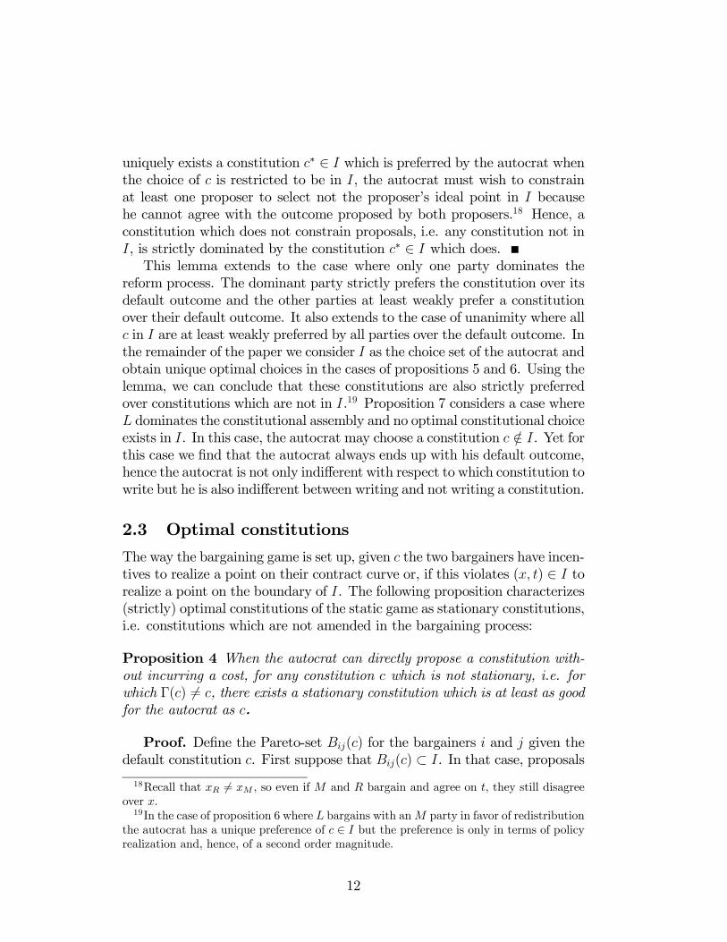
uniquely exists a constitution c∗ ∈ I which is preferred by the autocrat whenthe choice of c is restricted to be in I, the autocrat must wish to constrainat least one proposer to select not the proposer’s ideal point in I becausehe cannot agree with the outcome proposed by both proposers.18 Hence, aconstitution which does not constrain proposals, i.e. any constitution not inI, is strictly dominated by the constitution c∗ ∈ I which does.This lemma extends to the case where only one party dominates the

reform process. The dominant party strictly prefers the constitution over itsdefault outcome and the other parties at least weakly prefer a constitutionover their default outcome. It also extends to the case of unanimity where allc in I are at least weakly preferred by all parties over the default outcome. Inthe remainder of the paper we consider I as the choice set of the autocrat andobtain unique optimal choices in the cases of propositions 5 and 6. Using thelemma, we can conclude that these constitutions are also strictly preferredover constitutions which are not in I.19 Proposition 7 considers a case whereL dominates the constitutional assembly and no optimal constitutional choiceexists in I. In this case, the autocrat may choose a constitution c /∈ I. Yet forthis case we find that the autocrat always ends up with his default outcome,hence the autocrat is not only indifferent with respect to which constitution towrite but he is also indifferent between writing and not writing a constitution.

2.3 Optimal constitutions

The way the bargaining game is set up, given c the two bargainers have incen-tives to realize a point on their contract curve or, if this violates (x, t) ∈ I torealize a point on the boundary of I. The following proposition characterizes(strictly) optimal constitutions of the static game as stationary constitutions,i.e. constitutions which are not amended in the bargaining process:

Proposition 4 When the autocrat can directly propose a constitution with-out incurring a cost, for any constitution c which is not stationary, i.e. forwhich Γ(c) 6= c, there exists a stationary constitution which is at least as goodfor the autocrat as c.

Proof. Define the Pareto-set Bij(c) for the bargainers i and j given thedefault constitution c. First suppose that Bij(c) ⊂ I. In that case, proposals

18Recall that xR 6= xM , so even if M and R bargain and agree on t, they still disagreeover x.19In the case of proposition 6 where L bargains with anM party in favor of redistribution

the autocrat has a unique preference of c ∈ I but the preference is only in terms of policyrealization and, hence, of a second order magnitude.

12

coincide with points on the contract curve, i.e. Pi→j maximizes ui given uj(c)and Pj→i maximizes uj given ui(c). If one proposal P includes a lower valueof t than the other, the autocrat is better off by selecting this proposal Pinstead of c. Setting c = P guarantees that each proposer has to propose cwhen this is the default outcome. If the proposals Pi→j and Pj→i include thesame value of t, the autocrat is as well off if he selects either Pi→j or Pj→i

instead of c.Next suppose that Bij(c) ∩ I ( Bij(c). In that case, the constraint that

the proposal has to be in I may be binding. Yet a proposal P maximizesthe proposer’s utility given that it is in Bij(c) ∩ I. Note that Bij(c) ∩ I isconvex. When L or M is proposal maker, preferences of the proposal makerare strictly convex and the optimal proposal is uniquely defined. If this pointis selected as default, the constitution is stationary. If Rmakes a proposal thebinding segment of the boundary of I is strictly convex unless it coincideswith the t = 0-line.20 In either case, R has a unique proposal which, ifselected as default results in a stationary constitution21 and we are left withthree possibilities: a) In point P constraint Bij(c) is binding and I is not.This coincides with the case where Bij(c) ⊂ I. b) Constraint I is binding andBij(c) is not. In that case, with P the proposer realizes the highest utilityin I. If the autocrat selects c = P , either proposer must propose point cwhen it is the default outcome. c) Both constraints are binding. This casecoincides with case b).This proposition allows us to focus on stationary constitutions when look-

ing for optimal constitutions for the autocrat when discussing the static con-stitutional choice problem. In the dynamic constitutional choice problem,the autocrat incurs a cost when committing to a constitution and, as shownin the proof of proposition 9, proposition 4 does not apply.

3 Static constitutional choice

In this section we derive the optimal constitutional choice for the autocratif he believes that his demise is imminent. As we know from lemma 3, anydefault constitution c will be accepted by the bargainers. Yet only if theconstitution is in the set I, will it actually impact on the successor’s decision

20To see that R’s proposal is unique when the t = 0 line is binding, recall that by ourassumption that R’s preferences are lexicographic, R’s preferred point on the t = 0-line isuniquely determined. Hence, the optimal constitutional choice coincides with this point.21To see that the point c = (0, xR) is stationary when selected as default in the case

where t = 0 is the constraint on R’s proposal, observe that R as a responder will rejectany proposal which does not coincide with c.

13

other than by requiring them to propose amendments only in I. Hence weare going to focus on the autocrat’s constitutional choice as the problem ofpicking a constitution from within the set I. Finally, from proposition 4 weknow that we can focus on stationary constitutions, i.e. constitutions whichthe predecessors accept with no amendment.

3.1 M and L negotiate on constitutional reform

Suppose it is known that after transition M and L negotiate over constitu-tional reform and suppose in particular that this is known to the autocratwhen he writes the status quo constitution. From the perspective of the auto-crat’s clientele, the case where R is excluded as negotiator represents a worstcase scenario. So it is not implausible that, when writing the constitution,the autocrat focuses on that scenario in order to provide insurance againstits consequences.During the Egyptian revolution it was widely expected that it was ulti-

mately up to the street protesters and the Muslim brotherhood to negotiatethe future constitutional compact. If we identify the Muslim brotherhoodwith its welfare goals as the L party and the street protesters with theirmiddle class ambitions as the M party,22 we can explore the possible impactwhich the choices of an initial agenda setter - be it Mubarak or the military- would have had on the outcomes which the other two groups could haveobtained.

3.1.1 Case wM > w

Initially we suppose that the lower boundary of the set I intersects the ver-tical part of the contract curve between L and M . That the contract curveis a vertical line for 0 < t < 1 is demonstrated in the appendix. In that case,the autocrat wants to choose c∗ such that c∗ coincides with the intersectionof the lower boundary of I and the contract curve in figure 1. To see thelatter point, suppose that the autocrat picks a constitution at a point suchas z which also is on the boundary of I and corresponds to a lower tax t.As the boundary of I coincides with l0, M must realize a lower indifferencecurve mz. If L proposes, she will propose a higher tax at the point wherethe contract curve intersects with mz. This comes with a higher tax rate. IfM proposes, she will propose the point where l0 intersects with the contractcurve. Here the tax rate is the same as with c∗. Hence, as long as L pro-poses with positive probability, it is better to select c∗ in the point where l0

intersects with the contract curve.22See section 5 for a more detailed discussion of these claims.

14

We can exclude the case where the lower boundary of I intersects withthe upper horizontal part of the contract curve (i.e. where t = 1) becausethis would imply t0 = 1. So consider the case where the lower boundary ofI intersects with the lower horizontal part of the contract curve (i.e. wheret = 0). In that case, the autocrat may select any point on the horizontalpart of the contract curve and he will choose to select x ∈ [xM , xL] as closeas possible to xR. The two negotiators will necessarily propose the defaultoutcome c to each other. Naturally, also in the case where the optimalconstitution involves t∗ = 0, writing the constitution offers positive monetaryvalue to the autocrat because t0 > 0.[Insert Figure 1 here]

Proposition 5 In the static model with L andM as bargainers and wM > w,the autocrat strictly prefers handing down a constitution. The monetary valueof handing down a constitution is strictly positive.

Proof. See discussion above.

3.1.2 Case wM ≤ w

Next suppose that M has less than average effective wealth and, therefore,agrees with L on the ideal tax rate of t = 1. In that case which is illustratedin figure 2, negotiations between L and M will result in the maximum levelof redistribution which does not violate R’s participation constraint, i.e. thetax rate is t = t0, independently of the status quo constitution. To R, wholexicographically prefers wealth, the monetary value of writing a constitutionis zero yet he would still like to write a constitution in order to satisfy hispolicy preference with ideal point xR. If writing a constitution is costly interms of wealth, the autocrat prefers not to write a constitution.[Insert Figure 2 here]

Proposition 6 In the static model with L andM as bargainers and wM ≤ w,a constitution affects only policy but does not affect post transition wealth.Hence the monetary value of writing a constitution to the autocrat is zero.

Proof. See discussion above.

3.2 R and M negotiate on constitutional reform

In this section we assume that R and M are predicted to negotiate on con-stitutional reform. This was effectively the bargaining set up in the Chileantransition with the PN of the right and the moderate concertación negoti-ating transition. The ”Pinochet” constitution had banned left-wing parties

15

from political participation and their admission was one element of constitu-tional reform which emerged from the negotiations. It is, therefore, possibleto argue that the authors of the ”Pinochet” constitution had believed thatany successor government was not going to include parties of the left.

3.2.1 Case wM > w

In this case there is harmony betweenM and R on their redistributive goals.Yet L’s participation constraint has to be satisfied. Without further con-straints,M would choose her ideal point in I which is not the point with thelowest tax rate but a point on the contract curve with L. By strategicallychoosing the status quo constitution c∗ to coincide with point in I wheret is minimal, R can ensure a better outcome for himself: If M proposesagainst c∗, she has to offer t ≤ t∗ to R, so it must propose c∗ itself. And ifR proposes, he wants to propose c∗ as well. Therefore, equilibrium c∗ is astationary constitution.It is easy to see in figure 3 that a point such as z is not an optimal choice

for a status quo constitution: When R proposes he needs to offer M thepoint z again because there the tax rate is lowest given that M must obtainmz and L must obtain l0. When M proposes, she needs to offer the point zas well. Thus, z is also a stationary constitution but it is not optimal for theautocrat.Note that if L’s power to enforce outcomes in the conflict scenario is weak,

I may include the t = 0 axis. In that case, R and M will always agree ona tax rate of zero. The monetary value of writing a constitution is strictlypositive, as the reversion outcome in the absence of a constitution involvest0 > 0.[Insert Figure 3 here]

3.2.2 Case wM ≤ w

Finally consider the case where M has below average effective wealth andnegotiates with R. In that case, it is straightforward that R selects thestatus quo constitution c∗ by choosing the point in I where the tax rategets minimal. This case is illustrated in figure 4. Again, it is easy to checkthat this constitution is stationary. Moreover, the constitution has monetaryvalue to the autocrat because I is not vanishing by lemma 2 and, hence,t∗ < t0.[Insert Figure 4 here]

16

3.3 Other cases

For the case of negotiations between R and L, the choice of a constitutionfollows the same pattern as in the case of negotiations between R and M : Ifthe middle class has more than average effective wealth, c∗ is chosen in thepoint in I where the tax rate gets minimal (see figure 3). If M has less thaneffective average wealth, c∗ is again chosen in the point in I where the taxrate gets minimal (see figure 4).The same holds if a proposal in the constitutional bargaining game needs

approval of all three players. In that case, any selection of c ∈ I leavesno proposer with another possibility than proposing c. Hence, the autocratselects his preferred point in I, as in the case where R andM negotiate witheach other.To complete our exposition, suppose that one party is sufficient to carry

through constitutional reform. Majority rule may put one party in sucha position even when the other parties can prevent her from realizing herideal point in the conflict scenario. If the preexistence of a constitutionc is necessary to prevent descent into conflict, such a constitution wouldat least be weakly acceptable as a template to all players and it would bestrictly preferred by the player who stands to gain from the reform process.Moreover, if the dominant party selects a reform constitution within theconstitutional process, it will propose its preferred point in I. The questionfor the autocrat of whether to write a constitution now reduces to whetherthe dominant party will select t < t0 in the constitutional process. This isobviously the case when either M is predicted to be dominant and fulfillswM < w or when R is dominant. Hence, in those cases writing a constitutioncreates positive monetary value for the autocrat. On the other hand, if Lis predicted to be dominant, it offers M and R their reversion value whichputs them in no better place than with open conflict. Hence, incentives forwriting a constitution would completely vanish. The same applies to the casewhere M with wM > w is dominant. The following proposition summarizesour results:

Proposition 7 With negotiations between M and R or between L and Ror with all three players, writing a constitution always has positive monetaryvalue for the autocrat. If there is one dominant party in the constitutionalreform process, writing a constitution only has positive monetary value forthe autocrat in the cases where R is dominant or an M party opposed toredistribution is dominant. If L or an M party in favor of redistribution ispredicted to be dominant, the autocrat is indifferent between writing and notwriting a constitution.

17

4 A model of intertemporal constitutionalchoice

The previous section has introduced a static model of constitutional choicewhere the autocrat can choose the default constitution for his successorswithout incurring any cost such as being bound by the constitution himself.In practice, it is likely to be a condition for a constitution to be acceptablethat it actually has been adhered to for some time before the regime’s demise.In addition, the autocrat may not know the precise date of his demise and,therefore, will want to write and implement the constitution at a time whenthe probability that he will be in his post for another day is still greater thanzero. On the other hand, the consequences of successfully handing down aconstitution might be felt for a long time. Therefore, we think it is reasonableto assume that the autocrat will attach non zero weights to the cost which heincurs by not realizing his preferred policy outcome (0, xR) during the timefor which he has to abide by the constitution himself and to the gains hisconstituency realizes during the time when his successors deliver a preferredpolicy outcome. We assume, that depending on the expected length of timein both states and the discount rate of the autocrat, these weights assumethe values (1 − δ) and δ. Even though (1 − δ), which increases with thetime in office, may itself depend on the choice of the autocrat’s constitution,we ignore the possibility of such endogeneity. If the autocrat hands downa constitution, he choose the constitution (t, x) which gives him the highesttotal benefit, i.e. he maximizes

VR(t, x) = (1− δ)uR(t, x) + δuR(Γ(t, x)).

If he does not hand down a constitution, his total pay off is

VR(∅) = (1− δ)uR(0, xR) + δu0R.

By selecting a constitution c0 /∈ I which is not binding during his termin office, the autocrat can realize the same pay off as with no constitutionin the initial period and a pay off uR(Γ(c

0) ≥ u0R in the second period. Thelatter relationship follows because the successors want to choose a reformconstitution (t, x) ∈ I.23

In all cases, where the monetary value from writing a constitution inthe static model is strictly positive, there must exist a constitution whichthe autocrat strictly prefers writing if the weight of the future is sufficientlygreat:

23See the proof of lemma 3.

18

Proposition 8 If the weight of the future, δ, in the autocrat’s objective func-tion is sufficiently great, there is a binding constitution which the autocratstrictly prefers to hand down in all cases where there is a positive monetaryvalue to writing the constitution in the static model.

Proof. The autocrat can always choose to hand down the statically opti-mal constitution. For that constitution, the cost of commitment uR(x∗, t∗)−uR(0, xR) is finite and the benefit of commitment is strictly positive, i.e.uR(x

∗, t∗) − uR(Γ(c0 /∈ I) > 0 if, as we have claimed, there is a positive

monetary value to writing the constitution.In all cases where there is no positive monetary value to writing a consti-

tution the autocrat would only consider writing a constitution which is nonbinding during his term of office. This scenario comprises the cases wherewM ≤ w and L is dominant or bargains with M bargain and the case whereL or an M party in favor of redistribution is dominant in the succeedingassembly.Finally, even when choosing a binding constitution, the autocrat may not

necessarily want to choose the stationary, statically optimal constitution.At least in those case where the statically optimal constitution does notinvolve choosing the point in I where t gets minimal, i.e. in the case whereL is expected to negotiate with an M party opposed to redistribution, theautocrat faces a trade off between loosening the constraint during his term inoffice and creating stronger incentives for a low tax regime after his demise:

Proposition 9 In the case where L negotiates with M and wM > w thereexists a critical weight δ∗ such that if δ falls below that weight, the autocratcompromises on the statically optimal constitution.

Proof. Let pM be the probability that M proposes in the bargainingprocess. If the autocrat chooses the statically optimal constitution c∗, Mproposes c∗ and L proposes c∗. Now suppose that the autocrat chooses aconstitution with a slightly smaller tax rate such as z in figure 1. In thatcase, M continues to propose c∗, so the autocrat gets t∗ with a weight ofpMδ. If L proposes, she proposes t0|(t0, x0) in the intersection of mz and thecontract curve. t0 > t∗, hence the outcome is worse for R and it is weightedwith (1− pM)δ. However, tz < t∗, hence by choosing z, the autocrat realizesa better outcome with a weight (1 − δ). Hence, for δ → 0, c∗ results in ahigher value of VR and for δ → 1, z results in a higher value of VR.Obviously, for very small δ, the autocrat may not want to hand down a

constitution. Therefore, the critical weight δ∗ only becomes relevant if thedistance between t0 and the statically optimal constitution c∗ is sufficiently

19

large to induce the autocrat to write a constitution given δ∗. The followingproposition generalizes this insight on the desirability of writing a constitu-tion:

Proposition 10 The greater the power of R in the transition scenario and,hence, the smaller t0, the less value writing a constitution has.

Proof. In all cases where there is a monetary value of writing the consti-tution, the dynamically optimal constitutional choice c is independent of t0.Hence, R’s benefit of writing a constitution, uR(Γ(c))− uR(t

0) is increasingin t0, i.e. the smaller t0, the smaller the benefit. Finally, uR(Γ(c)) ≤ uR(t

0),hence the benefit must vanish as t0 → 0.

5 Application to different experiences of po-litical transition

From our analysis two hypotheses emerge.

1. If an autocrat expects that his own clientele will have influence ona succeeding constitutional assembly, he generally has incentives towrite a constitution, although those incentives vanish if he expects thatparties opposing redistribution will be able to impose their preferredpolicy without the left being able to object.

2. If an autocrat expects that his own clientele will have no influence ona succeeding constitutional assembly, he only has strong incentives towrite a constitution if he expects that the middle class prefers a lowredistribution policy.

In the case of the Chilean constitutional project, it seems plausible thatthe conditions for constitution writing in hypothesis 1 - negotiations betweenthe right and the middle class under a sufficiently strong perceived threat bythe left - have been met or were believed to be met by the autocrat. That theleft would not in a formal sense be involved in negotiations over a successorconstitution was plausible from the point of view of the old regime because itdid its utmost to keep it outside the political process. As it turned out, a sub-stantial part of the left also objected to accept the constitution as a vehicletowards political reform.24 If one accepts that one rationale of the Pinochetregime for embarking on the constitutional project was to build a bulwark

24For a dissenting view see Tapia (1987).

20

against communism, as suggested by Montes/Vial (2005), the possibility ofa left-wing threat must have been on the mind of the authors of the con-stitution. Protest movements such as the one led by copper miners in 1983(see Collier and Sater, 1996) and the so-called ”protesta” movement whichinvolved members of privileged, middle and working class (see O’Donnell andSchmitter, 1986) must have reminded the junta of such a lingering threat.An interesting question which remains is which the influence of middle

class wealth has been in the case of Chile’s successful constitutional transi-tion. The moderation which the parties of the concertación showed in thetransition process suggests that redistribution was not on the mind of themiddle class which it represented. In an accompanying paper we discuss therelationship between middle class wealth and stable transition in the Chileancase in greater depth (Michalak/Pech, 2012).It is more difficult to see to which case the Egyptian transition corre-

sponds. The Muslim brotherhood, with its social welfare goals probably bestfits the description of leftist in the context of our model. On the other hand,the often secular groups which started the street protests voiced aspirationswhich are more compatible with a middle-class mind set with an emphasison improvement of opportunities rather than the redistribution of existingwealth. Moreover, Egypt’s Gini coefficient is lower than Chile’s and the woo-ing of the presidential candidate of the right for the voters of this ”middleclass” further supports the view that Egypt best fits the case of a countrywith a middle class opposed to redistribution. This would give the autocratstrong incentives to write a constitution provided that he expects that theconstitutional reform process takes the form of multiparty bargaining. If,on the other hand, the expectation is that the Muslim brotherhood plays adominant role in the constitutional reform process, there is no value at all towriting a constitution.Therefore, the prediction of our model critically depends on the prior

about the bargaining strength of the different players in negotiating consti-tutional reform. In the case where the Muslim brotherhood is expected tobe dominant, we predict that no constitution will be handed down. In thecase where multiparty bargaining is expected to take place, we predict aconstitution will be handed down which might be significantly amended inthe bargaining process. Moreover, there are reasons why the monetary valueof constitution writing may be low even when the expectation is multipartybargaining: The autocrat may predict the military to be a strong playerwith significant power to enforce a high default outcome in any transitionprocess or he may predict a long time horizon of his rule. In these caseshe would have been reluctant to chose a constitution which binds his ownactions. Finally, it is unclear how to interpret the fact that the constitution

21

was formally revoked even by those players who would have stood to ben-efit to the extent that they expected to have a share in future bargainingover reform. An orthodox interpretation of this fact would be to say thatnon compliant constitutional practice during the autocracy turned out to bea bar to acceptability. However, our model suggests a second interpretationwhich is more in line with the observation that the property order establishedunder the constitution was kept in place. This observation would correspondto the case of stable constitutional transition but with major amendments.We lack observations where constitutional succession was tried in the face

of a middle class supporting redistribution. On the other hand, our modelpredicts that such cases would be rare to observe. What our model highlights,though, is the importance of established property rights as an element of con-stitutional arrangements which the autocrat wants to protect. This may sheda light on the failure of stable constitutional transition in the case of formercommunist countries. This was not completely for the lack of trying becauseat least in the case of Poland we observe a transition through pact betweenthe old and incoming power (see Munck and Leff, 1997). However, in thecase where a new constitution has to legitimize an emerging property order,the stakes are quite different from the cases discussed in this paper. Indeed,it will be more important for emerging property owners - often members ofthe former nomenclatura - to secure their share in the emerging propertyrights before they can think about securing those property rights within aconstitutional compact.

6 Further Discussion

The main lesson which emerges from the model and the preceding discussionis that handing down a constitutional compact offers benefits to the auto-crat’s clientele in almost all cases where multiparty bargaining is expectedduring the transition process: If a constitution is accepted by its successors,it provides insurance against being excluded from transition bargaining aslong as the middle class is opposed to redistribution and improves the bar-gaining position of the clientele relative to representatives of other classes.There is no such benefit if during transition one party is able to impose itspreferred outcome. This suggests that there are economic and political condi-tions which facilitate successful constitutional transition. If the middle classis sufficiently wealthy to oppose redistribution, it serves as a natural proxyfor the autocrat’s clientele during the transition process. Furthermore, onlyif society is sufficiently heterogeneous such that there are different groupswith diverging interests which find it necessary to reach compromise in the

22

transition process is there a role to play for any inherited constitutional tem-plate. The latter point suggests that transitions such as in Poland or inSouth Africa where Solidarnocz and the ANC emerged as main players wereless open to be manipulated by autocratic constitutional choice than thetransitions discussed in this paper.

References

[1] Barbera, S. and Jackson, M. O. (2004), Choosing How to Choose: Self-Stable Majority Rules and Constitutions, Quarterly Journal of Eco-nomics 119: 1011 - 1048.

[2] Barbera, S., Jackson, M.O. (2006), On the Weights of Nations: As-signing Voting Weights in a Heterogeneous Union, Journal of PoliticalEconomy 114: 317-339.

[3] Baron, D.P., Diermeier, D. (2001) Elections, Governments, and Par-liaments in Proportional Representation Systems. Quarterly Journal ofEconomics: 932-967.

[4] Barros, R. (2002), Constitutionalism and Dicatorship. Pinochet, theJunta, and the 1980 Constitution, Cambridge University Press, Cam-bride UK.

[5] Brown, N. (2011a), The Egyptian Constitution’s Rulebookfor Change, Foreign Policy, 3 February 2011, retrieved fromhttp://mideast.foreignpolicy.com/posts/2011/02/03/the_egyptian_constitution_s_rulebook_for_change.

[6] Brown, N. and Dunnes, M. (2011b), Egypts Draft ConstitutionalAmendments Answer Some Questions and Raise Others, Carnegie En-dowment for International Peace, 4 March 2011.

[7] Collier, S. and Sater, W.F. (1996), The History of Chile 1808-1994,Cambridge University Press, Cambridge, UK.

[8] Easterly, W. (2001), Middle Class Consensus and Economic Develop-ment, Journal of Economic Growth 6: 317-35.

[9] Egypt’s Freedom, Financial Times, 20 May 2012.

[10] Egypt court orders parliament dissolved, Financial Times, 15 June 2012.

23

[11] Gersbach, H., 2004. Why One Person One Vote? Social Choice andWelfare 23: 449-464.

[12] Grossman, H.J. (2002), Constitution or Conflict?, NBERWorking Paper8733.

[13] Kitschelt, H. (1996), The transformation of European Social Democracy,Cambridge University Press.

[14] Lagunoff, R. (2007), Dynamic Stability and Reform of Political Institu-tions, Games and Economic Behavior 67: 569-583.

[15] Michalak, M. and Pech, G. (2012), Strategic Constitutional Choice inan Autocracy: The 1980 Constitution in Chile.

[16] Montes, J. Esteban and Vial, T. (2005), The Constitution BuildingProcess in Chile: The Authoritarian Roots of a Stable Democracy, Inter-national Institute for Democracy and Electoral Assistance, Stockholm.

[17] Munck, G.L. and C.S. Leff (1997), Modes of Transition and Democrati-zation: South America and Eastern Europe in Comparative Perspective,Comparative Politics 29: 343-362.

[18] Myerson, R. (2008), The Autocrat’s Credibility Problem and Founda-tions of the Constitutional State, American Political Science Review102: 125-139.

[19] Naqvi, N., Neumaerker, K.J.B., Pech, G. (2012), The Rule of Lawand Sustainability of the Constitution, CEN Working Paper 02-2012,Freiburg.

[20] North, D. C., Weingast, B. (1989), Constitutions and Commitment:The Evolution of Institutions Governing Public Choice in SeventeethCentury England, Journal of Economic History 49: 803-832.

[21] Ordeshook, P. (1997), Constitutions for New Democracies. Reflectionsof Turmoil or Agents of Stability? Public Choice 90: 55-72.

[22] O’Donnell, G. and Schmitter, P.C. (1986), Transitions from Authori-tarian Rule. Tentative Conclusions about Uncertain Democracies, JohnHopkins University Press, Baltimore.

[23] Pech, G. (2009), Rationality and the Legal Order, in: Economics, Ra-tional Choice and Normative Philosophy, ed. by Tom Boylan and RuvinGekker, Routledge Series Frontiers of Political Economy.

24

[24] Przeworski, A., Wallerstein, M. (1988), Structural Dependence of theState on Capital, American Political Science Review 82: 12-29.

[25] Riker, W. (1986), The Art of Political Manipulation, Newhaven: YaleUniversity Press.

[26] Riker, W. (1996), The Strategy of Rethoric, Newhaven: Yale UniversityPress.

[27] Schofield, N. (2002), Evolution of the Constitution, British Journal ofPolitical Science 32: 1-20.

[28] Tapia, J. (1987), Sobre el uso de la ’legalidad’ de la dictatura, Cauce113 (22 June): 22-29.

[29] Tsebelis, G. (2002), Veto Players: How Political Institutions Work,Princeton University Press.

[30] Weingast, B. (1997), The Political Foundations of Democracy and theRule of Law, American Political Science Review 91: 245-263.

7 Appendix

In this appendix we show that in the case where L and M bargain andwM > w the contract curve is vertical for 0 < t < 1. For convenience, wedefine the income gap of each group relative to average available income as∆M = wM − w ≶ 0, ∆L = wL − w < 0 and ∆R = (1− γ)wR − w > 0.For 0 < t < 1, M ’s proposal PM→L = (t0, x0) given c = (t∗, x∗) solves the

constrained optimization problem

max[vM(x) + (1− t)wM + tw] s.t. vL(x) + (1− t)wL − tw ≥ u(t∗, x∗).

Writing μ(x0) =∂vM (x0)

∂x∂vL(x

0)∂x

≤ 0, the the first order conditions for an interiorsolution of this problem, x0 satisfies

μ(x0) =∆M

∆L(3)

and the tax rate is determined as the residual satisfying

t0 =vL(x

∗)− vL(x0)

(−1)∆L+ t∗. (4)

25

At xM , μ(xM→L) = 0 and at xL, μ(xM→L) → −∞. By continuity ofμ, a solution x0 satisfying the first order conditions uniquely exists withx0 ∈ [xM , xL). As ∂vM (x

0)∂x

= −2|x0 − xM | and ∂vL(x0)

∂x= 2|x0 − xL|, x0 only

depends on the ratio ∆M

∆L. By construction, x0 is the policy level which is

Pareto-optimal for L and M . Call this policy realization xe. It is easy toshow that L, when proposing to M selects the same policy xe.The optimal proposal can be interpreted as follows: xe is the policy which

would maximize the joint pay off for L andM given that transfers betweenMand L can only be achieved through the linear tax system: ∆M

∆Lis the rate at

whichM ’s income is converted into L’s income as the tax rate increases. Notethat a transfer rate of greater than −1 signifies an involuntary contributionof R.25 If the ratio is −1/2, it costs half a unit of M ’s income to increaseL’s income by one unit. μ is the rate at whichM ’s utility from consuming xincreases per unit of utility decrease by L. In an optimum, M ’s gain has tobe equal toM ’s cost of compensating L at an admissible tax rate t ∈ (0, 1).26

25One can show that the ratio is greater than −1 if wL+wM

2 < (wM − wL), i.e. if M ’swealth exceeds L’s wealth by more than average wealth, where the latter is calculatedlooking at M and L only. To demonstrate this point, note that ∆

M

∆L can be written aswM+(wM−wL)−wRwL−(wM−wL)−wR26If ∆M/∆L = −1, we obtain the familiar policy choice rule of selecting x half way

between the bliss points, see e.g. Baron/Diermeier (2002).

26

Figure 1: Optimum constitution when L is expected to negotiate with Mover reform and wM > w.

Figure 2: A constitution which guarantees a positive monetary value to Rdoes not exist when L is expected to negotiate with M over reform andwM ≤ w.

27

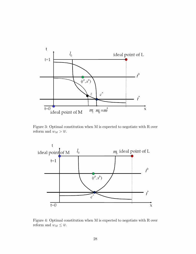
Figure 3: Optimal constitution when M is expected to negotiate with R overreform and wM > w.

Figure 4: Optimal constitution when M is expected to negotiate with R overreform and wM ≤ w.

28

Quandaries of Gridlock and Leadership in U.S.Electoral Politics

Evan Schnidman, and Norman Schofield

September 21, 2012

1 Introduction

The United States currently faces a number of severe political economic quan-daries. First is the economic quandary of debt. From 1993 to 2001, the USpublic debt to GDP ratio fell from 49% to 33% but has since risen to about100%. Entitlements, due to the aging “baby boom generation”will, in all likeli-hood, increase this ratio even more. The transformation to the global economycoupled with the internet revolution has changed the international structureof comparative advantage and has had a dramatic effect on employment pos-sibilities and on income and wealth distribution. China, India and Brazil aregrowing rapidly, and China’s propensity to save, coupled with its manipulatedcurrency has contributed to the US current account deficit, as well as facilitatedthe level of US public debt. The resulting uncertainties have induced violentswings in global stock markets. In the background is the fear of the effectsof global warming or “weirding”and concerns about how to deal with the USappetite for oil.1

Many people now fear that we face a repetition of the 1930’s. While the“Great Depression”may have started with the market collapse of 1929, it wasthe failure of the largest Austrian bank, Kreditanstalt, in 1931 that triggeredthe sequence of bank failures in Europe and the US, coupled with the Smoot-Hawley Tariff Act earlier in June 1930, that led to the enormous contraction ofworld trade and deepening of the crisis.2

As Keynes (1936:380) made clear“at the cost of the enlargement of the functions of government [to involve] the

task of adjusting to one another, the propensity to consume, and the inducementto invest” the liberty and effi ciency of the world economy could be preservedand enhanced.

1Too many books to name have addressed these quandaries, but we can mention Gal-braith (2008), Reich (2010), Milanovic (2010), Friedman and Mandelbaum (2011), Harvey(2011), Lessig (2011), Rachman (2011), Sachs (2011) and Steyn (2011), Buchanan( 2011),Noah (2012), Stiglitz (2012), Smith (2012).

2See also the work by Fisher (1933) on debt deflation as a fundamental cause of thedepression,

1

From Roosevelt’s inauguration on March 3 until June 16, 1933, he pushedthrough the beginnings of the New Deal, including the Emergency Banking Act,the Economy and Beer-Wine Revenue Act (finishing Prohibition, and providingmuch needed government revenue), the Agricultural Adjustment Act (to dealwith over production, but also with an amendment that essentially took the dol-lar off the gold standard), and the National Industrial Recovery Act ( althoughTitle I of the Act was deemed unconstitutional by the Supreme Court on May 27,1935). The CCC (Civilian Conservation Corps), the FERA (Federal EmergencyAuthority), the TVA (Tennessee Valley Authority), the NIRA (National Indus-trial Recovery Administration), the PWA (Public Works Administration) andthe AAA (Agricultural Adjustment Administration) were all created to attemptto deal with unemployment, partly through public works. In June 16, 1933, theGlass—Steagall Act had established the Federal Deposit Insurance Corporation(FDIC) in the United States and introduced banking reforms, some of whichwere designed to control speculation. Regulation Q allowed the Federal Reserveto regulate interest rates in savings accounts. Although these policy moves pre-dated Keynes’s book, they were consistent with some of Keynes’s earlier ideas.(Keynes, 1930a,b, 1933). Keynes himself had written to the President in 1933to praise him as a “trustee of the social system”and met with him later in May1934. Keynes later wrote to Roosevelt in 1938 recommending public ownershipof the utilities, nationalization of the railroads and subsidies for housing.The severe economic downturn in 1937, caused partly by attempts to balance

the budget, led to a Republican gain of 81 seats in the House and 6 seats inthe Senate in the 1938 election. The Fair Labor Standards Act (FLSA) of June25,1938, just prior to the election, was the last of the New Deal legislation.In a presentiment of the 1960’s, Roosevelt also faced opposition from southernDemocrats and had to give way on an anti-lynching bill. As Kennedy (1999:343) notes,“Roosevelt judged and the six week filibuster confirmed [that a frontal as-

sault on the South’s racial system] would irretrievably alienate the white south-ern establishment beyond repair and indefinitely deadlock the Congress.”However, the various efforts, prior to 1938, to regulate the economy eventu-

ally paid off in a significant increase in real US GDP as well developments innew technologies and large increases in factor productivity (Field, 2003; Allen,1994). These productivity increases may have been due to the ability of largecorporations to increase output even when reducing labor input. Livingston(2011) provides a good argument that the New Deal had reversed the earlierpattern of increasing income inequality and reanimated consumer led growth.(If this argument is correct, then it suggests a way out of the consequences ofthe current Great Recession.)The period from the collapse of democracy in Europe in the 1930’s to the

end of World War II led to major works of political economy by Von Mises(1940), Schumpeter (1942), Von Hayek (1944) and Popper (1945) that are stillbeing debated today.Fearful of another collapse, by the close of World War II, Keynes was arguing

for a clearing Union, with assets of the order of $500 billion in current terms.

2

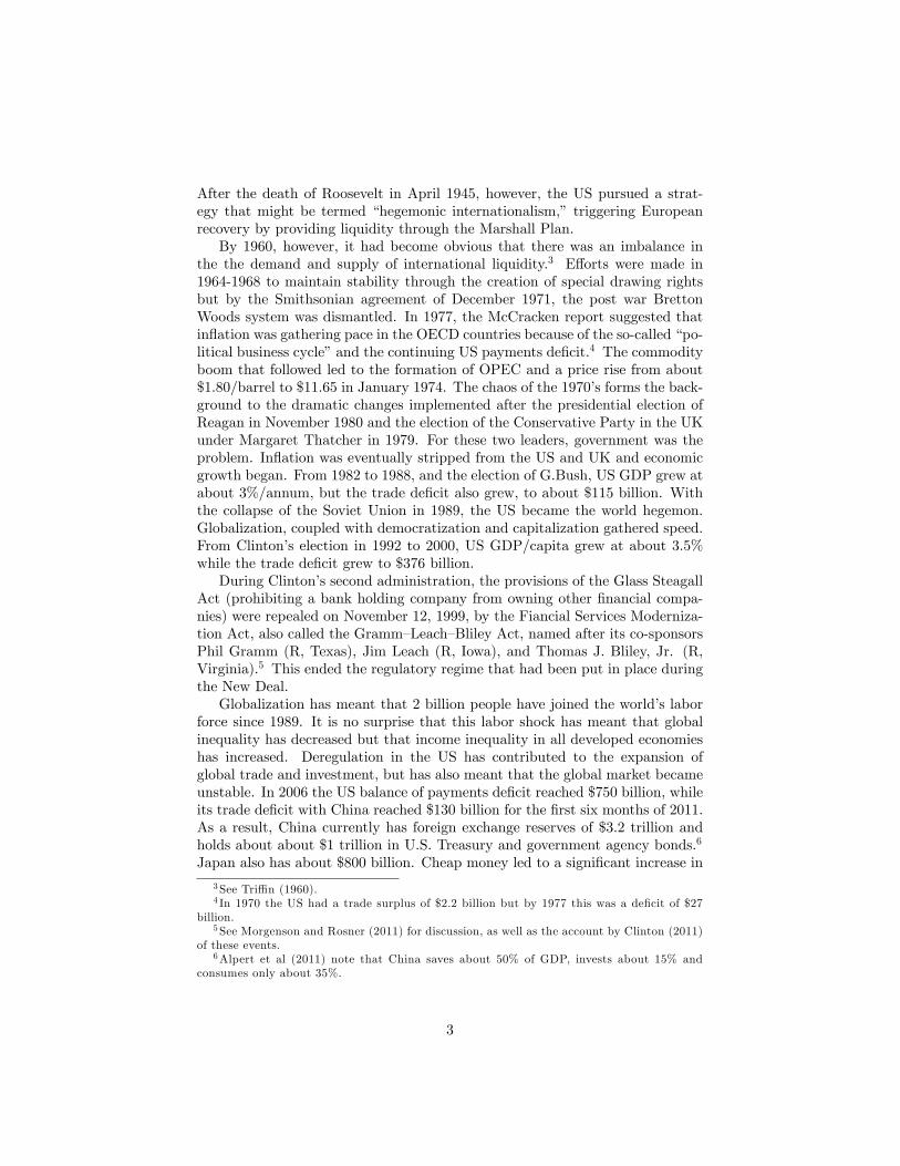
After the death of Roosevelt in April 1945, however, the US pursued a strat-egy that might be termed “hegemonic internationalism,” triggering Europeanrecovery by providing liquidity through the Marshall Plan.By 1960, however, it had become obvious that there was an imbalance in

the the demand and supply of international liquidity.3 Efforts were made in1964-1968 to maintain stability through the creation of special drawing rightsbut by the Smithsonian agreement of December 1971, the post war BrettonWoods system was dismantled. In 1977, the McCracken report suggested thatinflation was gathering pace in the OECD countries because of the so-called “po-litical business cycle”and the continuing US payments deficit.4 The commodityboom that followed led to the formation of OPEC and a price rise from about$1.80/barrel to $11.65 in January 1974. The chaos of the 1970’s forms the back-ground to the dramatic changes implemented after the presidential election ofReagan in November 1980 and the election of the Conservative Party in the UKunder Margaret Thatcher in 1979. For these two leaders, government was theproblem. Inflation was eventually stripped from the US and UK and economicgrowth began. From 1982 to 1988, and the election of G.Bush, US GDP grew atabout 3%/annum, but the trade deficit also grew, to about $115 billion. Withthe collapse of the Soviet Union in 1989, the US became the world hegemon.Globalization, coupled with democratization and capitalization gathered speed.From Clinton’s election in 1992 to 2000, US GDP/capita grew at about 3.5%while the trade deficit grew to $376 billion.During Clinton’s second administration, the provisions of the Glass Steagall

Act (prohibiting a bank holding company from owning other financial compa-nies) were repealed on November 12, 1999, by the Fiancial Services Moderniza-tion Act, also called the Gramm—Leach—Bliley Act, named after its co-sponsorsPhil Gramm (R, Texas), Jim Leach (R, Iowa), and Thomas J. Bliley, Jr. (R,Virginia).5 This ended the regulatory regime that had been put in place duringthe New Deal.Globalization has meant that 2 billion people have joined the world’s labor

force since 1989. It is no surprise that this labor shock has meant that globalinequality has decreased but that income inequality in all developed economieshas increased. Deregulation in the US has contributed to the expansion ofglobal trade and investment, but has also meant that the global market becameunstable. In 2006 the US balance of payments deficit reached $750 billion, whileits trade deficit with China reached $130 billion for the first six months of 2011.As a result, China currently has foreign exchange reserves of $3.2 trillion andholds about about $1 trillion in U.S. Treasury and government agency bonds.6

Japan also has about $800 billion. Cheap money led to a significant increase in

3See Triffi n (1960).4 In 1970 the US had a trade surplus of $2.2 billion but by 1977 this was a deficit of $27

billion.5See Morgenson and Rosner (2011) for discussion, as well as the account by Clinton (2011)

of these events.6Alpert et al (2011) note that China saves about 50% of GDP, invests about 15% and

consumes only about 35%.

3

household debt in the US, rising from about 65% of GDP in 1995 to 100% ofGDP in 2009.In a deregulated world, and in a context of moral hazard, financial institu-

tions competed for profits, speculating in risky assets, particularly derivativesbased on the housing market. The presumption that the market could regulateitself proved unfounded, just as Minsky (1986) has argued. This imbalance canlead to the kind of instability that Keynes feared.

If I may be allowed to appropriate the term speculation for theactivity of forecasting the psychology of the market, and the termenterprise for the activity of forecasting the prospective yield of as-sets over their whole life, it is by no means always the case thatspeculation predominates over enterprise. As the organization ofinvestment markets improves, the risk of the predominance of spec-ulation does, however, increase . . . Speculators may do no harm asbubbles on a steady stream of enterprise. But the position is seriouswhen enterprise becomes the bubble on a whirlpool of speculation.(Keynes, 1936: 158-9)

Lehman Brothers did file for bankruptcy on September 15, 2008, and thebubble burst. The market crash has left the US with a public debt of about $15trillion. US household net worth fell from about $70 trillion in 2007 to about$50 trillion in 2009.7 Even in the year from June 2010 to 2011 house values fellby $1 trillion, and about 15 million homeowners find themselves owing morethan their homes are worth.The contagion spread to Europe, where the debt overhang meant that many

states found themselves at risk of default. The EU was forced to put togetherthe European Financial Stability Fund (EFSF) rescue package of €750 billion,able to issue bonds for up to € 440 billion for support to Euro member statesin diffi culty, including Greece, Italy, Ireland, Greece, Spain and Portugal. 8 .European banks were also at risk, holding over $2 trillion in risky sovereigndebt.A number of EU governments have fallen because of opposition to the aus-

terity measures imposed by the European Union, in order to deal with the debtcrisis. First, the Irish Parliament was dissolved on February 1, 2011, and anelection held on February 26. From 78 seats in 2007, the governing party, Fi-anna Fail, only took 25, and Enda Kenny of the opposition party, Fine Gael,became Taoiseach (Prime Minister) of Ireland on 9 March.In the 2011 general election in Finland, the Centre Party, led by Prime Min-

ister, Mari Kiviniemi, lost 16 of the 51seats that they had held, while the TrueFinns party gained 34 seats. The centre-right National Coalition Party, underJyrki Katainen, became the largest party for the first time. After long and

7Alpert et al (2011).8The European levels of total public debt/GDP currently are: Greece 166%, Italy 121%,

Ireland 109%, Portugal 106%, Belgiun 96%, Germany 83%, France 87%, Britain 80%, Spain56%.

4

diffi cult negotiations, Katainen was elected Prime Minister by the Finnish Par-liament on 22 June 2011, leading a coalition of six parties (National Coalition,Social Democrats, Left Alliance, Greens, Swedish People’s Party and ChristianDemocrats).Then the Prime Minister of Portugal, Jose Socrates, of the Socialist Party,

resigned on March 23, and the caretaker government obtained a bailout of $116billion on May 3, 2011. In the election of June 5, the center right Social De-mocrats, under Pedro Passos Coelho, took 39% of the vote to 28% for Socialistsand 12% for the Popular Party. Coelho will lead a coalition with the PopularParty, and promised further austerity measures to deal with the crisis.Lars Løkke Rasmussen, leader of the centre-right liberal party, Venstre, lost

his position as Prime Minister of Denmark in the September 2011 parliamentaryelection. He remained in offi ce as head of a caretaker government until hissuccessor, Helle Thorning-Schmidt, was appointed on 3 October 2011.Iveta Radicová was the leader of the Slovak Democratic and Christian Union

—Democratic Party, and Prime Minister of Slovakia from 8 July 2010 as thehead of a four-party center-right coalition government. Radicová lost a vote ofconfidence in the parliament on 11-12 October, 2011, leading to the fall of hergovernment. An early election will be held on 10 March, 2012.On November 5, 2011, the Greek Prime Minister, George Papandreou, agreed

to step down to make way for a unity government, and on November 10, Lu-cas Papademos became interim prime minister. In the election of May 6 2012,both major parties, PASOK, the center left party, only won 41 seats with 14%of the vote, while the center right , New Democracy took 108 seats with 18%of the vote. These reverses were seen as a rejection of the austerity measures,imposed by the EU. Of greater importance was the defeat of Nicolas Sarkozyin the second round of the French Presidential election, also on May 6 by thesocialist candidate Francois HollandeOn November 12,2011 the Italian Prime Minister, Silvio Berlusconi, had

resigned after Parliament approved a number of measures to reduce the deficit.Italy’s president then asked Mario Monti, a former European Commissioner, toform a government.José Luis Rodríguez Zapatero, the leader of the Spanish Socialist Workers’

Party (PSOE), was elected for terms as Prime Minister of Spain in the 2004 and2008 general elections. In the election of November 20, 2011, the conservativePeople’s party (PP) led by Mariano Rajoy won 186 of the 350 seats in parlia-ment, with a 44% vote and a mandate to carry out further austerity measures.Even Belgium found itself in diffi culty, with a debt to GDP ratio of 96%,

No coalition government had been able to form after the election of June 2010,because of conflicts between Flanders and Wallonia.. Eventually on December1, 2011, the downgrading of Belgium’s sovereign debt forced a coalition of sixparties to reach a tentative agreement to form a government under the SocialistParty leader, Elio Di Rupo.In fact the first political effects of the debt crisis were the fall of the Labour

government in the United Kingdom in May 2010 and the defeat of the Republi-can administration in the US in November 2008. The Conservative government

5

in the UK dealt with its debt problem by an intervention of the order of 13% ofGDP by the Bank of England. In the US the intervention by the Federal Re-serve has been of order 11% of GDP. In contrast the EU intervention has beenlimited to about 2% of EU GDP, which is why the euro debt crisis continues todestabilize bond markets.The complex web of the global economic crisis has created a great deal of

uncertainty in the market as well as in the political systems of both Europeand the United States. In Europe there is much debate whether the eurozonecan be sustained, though on December 9, 2011, twenty-six of the twenty-sevenmember states (all but the UK) agreed to a deepening of the EU. However, theelection defeats in Greece and France in May may have changed the emphasison the fiscal austerity strategy of German Chancellor Angela Merkel. Muddlingmatters further is the rising debt default threat in Italy and Spain which hascreated continued market unrest and political ambivalence.In the United States, this uncertainty coupled with decades of rising income

and wealth inequality has resulted in increased political volatility and partisanstrife. The indebted EU polities have electoral systems based on proportionalrepresentation, and as a result, government requires coalition agreement. Indeedthe formal model (Schofield, 2007) underlying this paper suggests that, underproportional representation, smallparties will generally adopt positions far fromthe center. This political polarization sustains fragmentation and governmentalinstability. In contrast the theory we use here suggests that "first past the post"or plurality electoral system of the US generates a strong convergent electoral ef-fect on political candidates, similar to the Downsian median voter result (Downs1957). We discuss recent events since the 2008 presidential election, and arguethat candidates do not adopt centrist policies. Instead, money has played anincreasingly important role in recent elections. Because of the two dimension-ality of the policy space, activists have been able to exert a centrifugal force onthe policy positions of the parties. As a result US politics is now characterizedby legislative gridlock. Indeed the increase in partisan rancor resulting from theneed to deal with federal debt of over $14 trillion has highlighted the extremelack of convergence in U.S. partisan politics.The remainder of this paper seeksto explain this centrifugal tendency in the 2008 and 2010 election cycles in theUnited States.

2 Activist Politics

2.1 The logic of the argument

Wise government should be able to address the quandaries described above.Madison’s logic in Federalist X (Madison [1787] 1999) was that a Republic couldexhibit a “probability of a fit choice”, suggesting that voters would make theirchoices on the basis of judgements rather than simply interests.In this paper we argue that the US polity is currently unable to make wise

decisions due to a structural defect that Jefferson feared could occur in the US.

6

Jefferson followed the arguments of Henry St. John, Viscount Bolingbroke, thatthe noble constitution of England had been destroyed by the crass commercial-ization and corruption of the Whig ascendency in the 1720s. Jefferson believedthat the opening of Hamilton’s First Bank of America in 1791 would also allowcapital to corrupt. He fought and won the election of 1800 to preserve the “Em-pire of Liberty”.9We can put this conflict in the more general context of rivalphilosophical systems of belief, as suggestsed by Israel (2012), who has pointedout that the modern period since 1700 witnessed a conflict between a "Radi-cal" Enlightenment espoused by Bolingbroke, Condorcet, Jefferson and Paine,in support of reason and equality and opposed to monarchy and hierarchicalhegemony, and the compromising "Moderate" Enlightenment of Hamilton andBurke. The importance of the social dimension in US politics, as discussd below,suggests that this conflict is as important as ever.10

In the early 20th century both Teddy Roosevelt and Wooodrow Wilson hadcontested the 1912 presidential election as Progresssives, opposed to the powerof commercial interests and the increasing economic inequality that had resulted(Gould, 2008). Indeed Chace (2004) suggests that the difference between Roo-sevelt and Wilson was that Wilson espoused a Jeffersonian belief in liberty andcompetition (through free trade etc.) while Roosevelt believed in a Hamiltonianacceptance, but regulation, of industrial capitalism.The thesis of this paper is that just as in 1800, in 1912 and in 1932, the US

faces a quandary that is essentially constitutional and involves the interrelation-ship between the polity and the economy. There are a number of componentsto the current quandary:(i) The election of L.B.Johnson in 1964 was the beginnings of a new “political

realignment”that involved the social dimension of civil rights as well as the usualeconomic dimension involving taxes and the like.11 We use factor analysis toconstruct these two dimensions. The social axis involves attitudes to AfricanAmericans, abortion, civil right for gays, traditional values and equality. Theeconomic axis involves government services, size of government, health care, apreference for the market over government and a belief that welfare expenditureshould be decreased. As Putnam and Campbell (2010) have shown, religiosityof voters is related to many of the beliefs that characterize the social axis. Thesecond axis has become more important over time, and we use the term socialactivists for activists on this axis. The principal consequence of this realignmenthas been the gain of the South by the Republican Party. Indeed, Reagan wonthe 1980 Presidential election as a result. The Republicans also gained both

9Kramnick (1990, 1992). See also Lind (2012) for the continuing conflict between theJeffersonian and Hamiltonian visions of the development of the USA political economy. Lindgives a detailed account of the logic of using resources generated by tariff protection to in-duce infrastructural improvements such as railways and canals, facilitating the industrialdevelopment of the Northern states.10See also the recent books by Crick (1995), Hitchens(2007), Dawkins(2000, 2011).11See Caro(2012) for a discussion of how LBJ was able to force through the civil rights leg-

islation in 1964 against Southern Democrat opposition in Congress. The gridlock in Congressin 1964 over this issue combined with partisan conflict over the budget has some similarity tothe current gridlock in Congress, discussed in this paper.

7

Houses of Congress in 1994.12 The change in the regulatory regime that hasoccurred in the last 30 years is a consequence of this realignment.(ii) Although the social axis has become electorally more important, eco-

nomic growth before the bursting of the balloon has increased the ability of thosewith economic assets to influence elections. We term these economic activists.Increasing income and wealth inequality has contributed to the enhanced powerof these activists. Indeed, an arms race between the parties has also increasedactivist power. At the same time, the significant benefits that have accrued toeconomic activists have led to a radicalization of economic activist preferences.By this we mean that their preferences, in comparison to the distribution ofelectoral preferences, have become more extreme.13

The Supreme Court decision, Citizens United v. Federal Election Commis-sion, on January 21, 2010, removed many restrictions on the money that couldraised for political campaign and in essence deregulated elections. This meansthat activists previous constrained to providing small amounts of cash and/orvolunteer time are now able to provide large sums of money to pay for largemedia buys and thousands of man-hours of electoral activism.(iii) The existence of two political dimensions has meant that it is possible

for winning coalitions to be contructed that combine both axes. In paricular,the Republicans have benefitted from a coalition of conservative economic andconservative social activists. This has led to dramatic differences in the patternof voter characteristics in states that tend to vote Democrat in contrast to thosewho tend to vote Republican.14

(iv) Models of elections are typically based on voter preferences alone. Re-cent studies of US elections (Clarke et al 2009, 2011) have emphasized theelectoral peception of the character traits of candidates. Such perceptions canbe influenced by the media, and in turn therefore by the money that candidatesspend. We suggest this provides the logic for the arms race between candidates.(v) Acemoglu and Robinson. (2008) have discussed the ability of elites to

exert de facto power in order to collect economic rents thus inducing ineffi cienciesin the political economy. Earlier work by Olson (1982) also focused on the abilityof interest groups, such as labor, to exert undue influence because of the natureof the democratic machinery. The model that we propose suggests that the defacto elite power is a result of a kind of rent seeking that occurs in the contextof a political prisoners’dilemma.(vi) The influence of money and the polarization within Congress suggests

that at the heart of the political quandary is a need to reconsider the constitu-tional separation of powers in the US.15

In the rest of the paper we consider models of US Presidential elections for

12See Schofield, Miller and Martin (2003), Schofield and Miller (2003) and Schofield (2007)and Schofield and Miller (2007) for a discussion of this realignment. See also Micklethwaiteand Wooldridge (2004) for a discussion of the changes in ideology and electoral support forthe Republican party in this period.13See Abramowitz and Saunders (2005) and Abramowitz (2010).14Abramowitz and Saunders (2005), Gelman (2008).15Posner and Vermeule (2011).

8

2000 to 2008, and then discuss the details of the contest between Obama andCongress over the last three years in order to gauge the validity of the aboveargument.

2.2 Modeling Elections

As we have noted, the formal literature on electoral competition has tended tofocus on preferences rather than judgements. Models of two-party competitionhave typically been based on the assumption that parties or candidates adoptpositions in order to win, and has inferred that parties will converge to theelectoral median, under deterministic voting in one dimension (Downs, 1957;Hotelling 1929), or to the electoral mean in stochastic models.16 These modelsof political convergence at least imply that political choice lead to a moderate orcentrist outcome. On the contrary, there is extensive evidence that politics hasbecome polarized with the two major parties far removed from one another.17

In this paper we consider a theory of political choice which accounts for po-larization in terms of activist influence. To do this, we first offer evidence thatthe political space is at least two dimensional. The nature of this policy spacecan be inferred for recent elections from voter surveys. For example, Figure 1presents an estimate of the distribution of voter preferences (or preferred posi-tions) in the U.S. presidential election of 2004.18 The first-left right dimensionrepresents preferences (or attitudes) towards government expenditure and taxesand can be interpreted as a economic axis.19 The second north-south or socialdimension reflects attitudes on social policy, particularly civil rights, as wellas voter opinions about abortion etc.20 Figure 1 also shows estimates of thepositions of the two presidential candidates.[Insert Figure 1 here]Because the political space is two-dimensional, parties in the United States

must be coalitions of opposed interests. Figure 1 also shows a partisan cleavageline obtained from a simple logit model of the 2004 Presidential election. Thiscleavage line joins the preferred points of voters who, according to the logitmodel, would choose the candidates with equal probability of one half. Thelogit model gives

ρdem ==exp(a+ bxi + cyi)

1 + exp(a+ bxi + cyi)(1)

16See the earlier work by Enelow and Hinich (1989), Erikson and Romero (1990) and morerecent work by Duggan (2006), and Patty, Snyder and Ting (2009).17See the works by Fiorina et al. (2005, 2009) and McCarty, Poole, and Rosenthal (2006)

on polarization in the electorate and Layman et al. (2010) on polarization among activists.18This figure is based on factor analysis of the American National Election Study (ANES)

for 2004. In the next section we give more details on the factor model that we used for the2004 and 2008 Presidential elections.19The economic axis is defined so that voters who believe in the free market and that

spending on welfare programs should be decreased are located on the right of this x− axis.20The social axis is defined so that voters who support civil rights for gays and believe that

abortion should be readily available are located to the north of this y − axis.

9

with (a, b, c) = (−0.2, 1.34,−0.93). Setting ρdem = 12 we obtain the equation

y = 1.44x− 0.21. (2)

This equation almost passes through the point (0,−0.21) and suggests thatthe Democrat candidate, Kerry, had a slight advantage over the Republicancandidate, Bush. This partisan cleavage line separates respondents who tendto vote Democrat, and generally are located in the upper left quadrant, fromthose who tend to vote Republican, in the lower right quadrant.Figure 2 shows the mean positions of Democratic and Republican Party vot-

ers and activists.21 Figure 2 suggests that though the Republican party containsboth socially conservative and socially liberal groups, almost all Republican ac-tivists are located in the lower right of the policy space. In opposition, all theDemocrat party activists tend to be located in the upper left of the policy space.The mean activist estimates are Act : 2004 Re p Dem

x 0.55 −0.49y −0.48 +0.75

(3)

The two dimensionality of the political space is corroborated by work in so-cial psychology that finds that there are in essence four "quadrants" to morality:Liberal secularists (upper left), the religious left (lower left), Libertarians (upperright) and social conservatives (lower right). The social psychological literaturedefines the left hand domain in terms of an emphasis on justice while the righthand domain is defined in terms of authority 22 .[Insert Figure 2 here]An analysis for the 2000 contest between Gore and Bush gives a similar

result with a partisan cleavage line given by

y = 1.87x− 0.34. (4)

Figures 3 and 4 show the distribution of voter and activist preferred positionsfor the 2008 election. For this election, the partisan cleavage line is given bythe equation

y = 0.82x− 0.4. (5)

which passes through the point (0,−0.4). This cleavage line suggests thegreater advantage of the Democrat candidate, Obama, over McCain. Notice

21The figure shows the standard error bars for these estimates, with larger error bars foractivist estimates.22More precisely, Graham et al (2009) use factor analysis on five moral traits, including

"compassion", "fairness", "loyalty", "authority" and "purity". These define the four moralclusters. Mondak (2010) uses regression analysis to explore the effects of personality traitssuch as "openness", "conscientiousness", extraversion", "agreeableness" and "emotional sta-bility" on political choice. Using the 2006 Congressional Election Study (CES) he showsthat "openness" and "conscientiousness" are correlated with liberal / conservative ideologyrespectively. Moreover, "openness" is associated with agreement with legalised abortion andweakly associated with opposition to Federal income tax cuts. This analysis is suggestive ofa correlation between the two dimensional trait space and the two dimensional policy space.

10

that the cleavage lines from 2000 to 2004 to 2008 had rotated slightly, in aclockwise direction, suggesting that the social axis had become increasinglyimportant.Table 1a gives the two dimensional factor model based on the ANES 2008

Survey, while Tables 1b and Table 2 give the results of the estimates of meanpositions of voters, activists and the candidates in 2008.[Insert Figures 3 and 4 and Tables 1a,b and 2 here]The mean activist estimates are Act : 2008 Re p Dem

x 1.41 −0.20y −0.82 +1.14

(6)

A comparison of (3) and (5) provides some evidence that activist averagepositions have become more extreme between 2004 and 2008. One way tocheck this inference is to compare (3) and (5) in terms of the electoral stan-dard deviations obtained from the factor models for the two elections.23 Using(σx, σy) = (0.76, 0.76), (0.9, 0.91) for 2004 and 2008 respectively, this correctiongives

Act : 2004 Re p Demx/sd 0.72 −0.64y/sd −0.63 +0.99

, Act : 2008 Re p Dem

x/sd 1.56 −0.22y/sd −0.91 +1.26

(7)

The correction suggests that Republican activists have, on average, becomemuch more radical in their preferences in both axes relative to the averagedistribution of electoral preferences. In contrast, Democrat Party activists haveon average, become more moderate on the economic axis, and more radical onthe social axis.Performing the same calculation for non-activists for the parties we find: 2004 Re p Dem

x 0.30 −0.33y −0.28 +0.37

, 2008 Re p Dem

x +0.72 −0.17y −0.56 +0.36

(8)

2004 Rep Demx/sd 0.40 −0.43y/sd −0.37 +0.49

, 2008 Rep Demx/sd 0.80 −0.19y/sd −0.62 +0.40

(9)

Average voter positions for the two parties have therefore shifted somewhattowards the two opposed quadrants, but not as much as the activist meanpositions. The increasing dominance of “Tea Party” social conservatives inthe Republican Party, and indeed the fact that the Congressional Republicanpositions in the recent election of 2010 appeared to be fairly “radical” in thelower right quadrant of the political space, caused some prominent Republicansto consider a change of party allegiance to the Democrats. Shifts in the activist

23Details of the 2008 factor model is given in the next section.

11

coalitions for the two parties thus cause a transformation of the partisan cleavageline.This phenomenon appears to be a fundamental aspect of U.S. politics: as

activists on the “trailing edge”24 of the cleavage line change party allegiance,then the positions of the two parties shift. This can be interpreted as a clockwiserotation in the political space.We argue that the fundamental changes in voter choice result not only from

changes in the distribution of electoral preferences, but from the shifts in elec-toral perceptions about the competence and character traits of the politicalcandidates.25 These perceptions are influenced by the resources that the candi-dates command. In turn, these changes in perceptions are the consequence ofthe shifting pattern of activist support for the candidates. The essence of theunderlying model is that it attempts to endogenize the resources available tocandidates by modelling the contracts they can make with their supporting ac-tivists. The activists must solve their own optimization problem by estimatingthe benefit they receive from their contributions and deciding what resources tomake available to their chosen candidate.In recent years, the importance of activist contributions has increased, and

this has enhanced the influence of activist groups.26 The empirical and formalmodels that we discuss here provide a reason why electoral politics has becomeso polarized in the United States. This model of activist polarization accountsfor the “disappearing center” in politics (Gelman, 2010) and the paradox thatpoor states seemingly tend to vote Republican while rich states tend to voteDemocrat (Abramowitz (2010).27

Moreover, this polarization appears to have benefited the wealthy in societyand may well account for the increase in inequality in income and wealth distri-bution that has occurred over the last decade. (Hacker and Pierson 2006, 2010,Pierson and Skocpol, 2007).Essentially there is an arms race between candidates over these resources

due to a feedback mechanism between politics and economics. As the outcomeof the election becomes more important, activists become increasingly awarethat the resources they provide have become crucial to election victories, andthey become more demanding of their chosen candidates. Because of the offerof resources, candidates are forced to move to more radical positions, and polar-ization in candidate positions increases, even though there may be little change

24These would, on the one hand, be cosmopolitan, socially liberal but economically con-servative Republicans (in the upper right quadrant) or on the other hand, populist, sociallyconservative but economically leftist Democrats (in the lower left quadrant).25Below we present an empirical model that links electoral perceptions to candidate char-

acter traits such as moral, caring, knowledgeable, strong, honest, intelligent, optimistic.26 Indeed, Herrera, Levine and Martinelli (2008) observe that spending by parties in federal

campaigns went from 58 million dollars in 1976 to over 1 billion in 2004 in nominal terms. TheCenter for Responsive Politics estimates that election spending, including candidate spending,went from about $3.5 billion in 2000 to $4.6 billion in 2004 to $5.3 billion in 2008.27The recent 2011 census stated that the poorest state was Mississippi, followed by Arkansas,

Tennessee, West Virginia, Louisiana, Montana, South Carolina, Kentucky, Alabama and NorthCarolina. All these are Republican strongholds.

12

in the degree of polarization of the electorate.Over the long run we see two forces at work. First, the continuing “cir-

cumferential”realignment induced by a slow rotataion of the partisan cleavageline, as activists switch party allegiance. Secondly, a “radial”polarization thatoccurs at times of political quandary, caused by economic downturn or shocksto the global political economy, inducing a change in the distribution of voterprefereed points.In the next section we present an outline of the model that we use. In Sec-

tion 3 we discuss the effect of the 2008 election followed by Section 4 where wediscuss the midterm election of 2010 and the ensuing conflict between the Pres-idency and Republican groups in Congress. The last section makes some briefcomments about the viability of the constitutional balance between executiveand legislature in the United States.

3 An Outline of the Model.

In the standard spatial model, only candidate positions matter to voters. How-ever, as Stokes (1963, 1992) has emphasized, the non-policy evaluations, orvalences, of candidates by the electorate are equally important. In empiricalmodels, a party’s valence is usually assumed to be independent of the party’sposition, and adds to the statistical significance of the model. In general, va-lence reflects the overall degree to which the party is perceived to have shownitself able to govern effectively in the past, or is likely to be able to govern wellin the future (Penn, 2009).Over the last decade a new literature has developed that considers deter-

ministic or probabilistic voting models including valence or bias towards one orother of the candidates.28

Recent work has developed an empirical and formal stochastic electoralmodel based on multinomial conditional logit methods (MNL). In this model,each political candidate ,j, was characterized by an intrinsic or exogenous va-lence,λj. This model can be considered to be Downsian, since it was based ona pure spatial model, where the estimates of valence were obtained from theintercepts of the model. It was possible to obtain the conditions for existence of“a local Nash equilibrium”(LNE) under vote maximization for a parallel formalmodel using the same stochastic assumptions as the MNL empirical model. ALNE is simply a vector of candidate positions with the property that no candi-date make a small unilateral move and yet increase utility (or vote share).29

The mean voter theorem asserts that all candidates should converge to theelectoral origin.30 Empirical analyses of the 2004 and 2008 U.S. presidentialelections that are mentioned in this paper have corroborated the earlier work

28Adams (2001), Ansolabehere and Snyder (2000), Aragones and Palfrey (2002), Banks andDuggan (2005), Groseclose (2001) and McKelvey and Patty (2006).29A Nash equilibrium (NE) is a vector of candidate positions so that no candidate has a

unilateral incentive to deviate so as to increase vote share. Thus any NE must be a LNE.30The electoral origin is the mean of the distribution of voter preferred points.

13

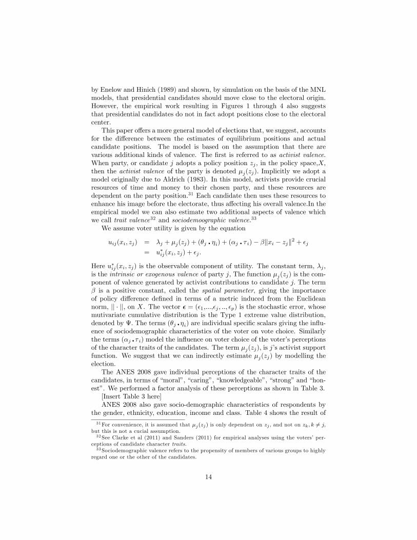
by Enelow and Hinich (1989) and shown, by simulation on the basis of the MNLmodels, that presidential candidates should move close to the electoral origin.However, the empirical work resulting in Figures 1 through 4 also suggeststhat presidential candidates do not in fact adopt positions close to the electoralcenter.This paper offers a more general model of elections that, we suggest, accounts

for the difference between the estimates of equilibrium positions and actualcandidate positions. The model is based on the assumption that there arevarious additional kinds of valence. The first is referred to as activist valence.When party, or candidate j adopts a policy position zj , in the policy space,X,then the activist valence of the party is denoted µj(zj). Implicitly we adopt amodel originally due to Aldrich (1983). In this model, activists provide crucialresources of time and money to their chosen party, and these resources aredependent on the party position.31 Each candidate then uses these resources toenhance his image before the electorate, thus affecting his overall valence.In theempirical model we can also estimate two additional aspects of valence whichwe call trait valence32 and sociodemoographic valence.33

We assume voter utility is given by the equation

uij(xi, zj) = λj + µj(zj) + (θj � ηi) + (αj � τ i)− β‖xi − zj‖2 + εj

= u∗ij(xi, zj) + εj .

Here u∗ij(xi, zj) is the observable component of utility. The constant term, λj ,is the intrinsic or exogenous valence of party j, The function µj(zj) is the com-ponent of valence generated by activist contributions to candidate j. The termβ is a positive constant, called the spatial parameter, giving the importanceof policy difference defined in terms of a metric induced from the Euclideannorm, || · ||, on X. The vector ε = (ε1,...,εj , .., εp) is the stochastic error, whosemutivariate cumulative distribution is the Type 1 extreme value distribution,denoted by Ψ. The terms (θj � ηi) are individual specific scalars giving the influ-ence of sociodemographic characteristics of the voter on vote choice. Similarlythe terms (αj � τ i) model the influence on voter choice of the voter’s perceptionsof the character traits of the candidates. The term µj(zj), is j’s activist supportfunction. We suggest that we can indirectly estimate µj(zj) by modelling theelection.The ANES 2008 gave individual perceptions of the character traits of the

candidates, in terms of “moral”, “caring”, “knowledgeable”, “strong”and “hon-est”. We performed a factor analysis of these perceptions as shown in Table 3.[Insert Table 3 here]ANES 2008 also gave socio-demographic characteristics of respondents by

the gender, ethnicity, education, income and class. Table 4 shows the result of31For convenience, it is assumed that µj(zj) is only dependent on zj , and not on zk, k 6= j,

but this is not a cucial assumption.32See Clarke et al (2011) and Sanders (2011) for empirical analyses using the voters’per-

ceptions of candidate character traits.33Sociodemographic valence refers to the propensity of members of various groups to highly

regard one or the other of the candidates.

14

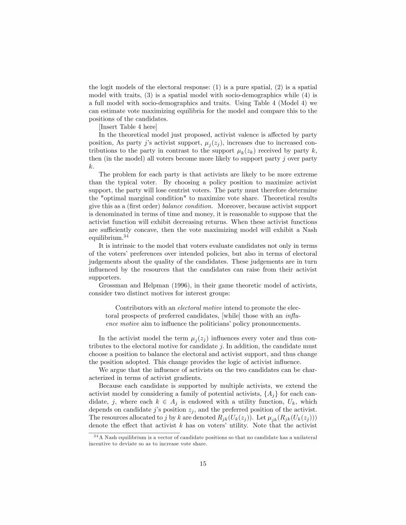
the logit models of the electoral response: (1) is a pure spatial, (2) is a spatialmodel with traits, (3) is a spatial model with socio-demographics while (4) isa full model with socio-demographics and traits. Using Table 4 (Model 4) wecan estimate vote maximizing equilibria for the model and compare this to thepositions of the candidates.[Insert Table 4 here]In the theoretical model just proposed, activist valence is affected by party

position, As party j’s activist support, µj(zj), increases due to increased con-tributions to the party in contrast to the support µk(zk) received by party k,then (in the model) all voters become more likely to support party j over partyk.The problem for each party is that activists are likely to be more extreme

than the typical voter. By choosing a policy position to maximize activistsupport, the party will lose centrist voters. The party must therefore determinethe "optimal marginal condition" to maximize vote share. Theoretical resultsgive this as a (first order) balance condition. Moreover, because activist supportis denominated in terms of time and money, it is reasonable to suppose that theactivist function will exhibit decreasing returns. When these activist functionsare suffi ciently concave, then the vote maximizing model will exhibit a Nashequilibrium.34

It is intrinsic to the model that voters evaluate candidates not only in termsof the voters’preferences over intended policies, but also in terms of electoraljudgements about the quality of the candidates. These judgements are in turninfluenced by the resources that the candidates can raise from their activistsupporters.Grossman and Helpman (1996), in their game theoretic model of activists,

consider two distinct motives for interest groups:

Contributors with an electoral motive intend to promote the elec-toral prospects of preferred candidates, [while] those with an influ-ence motive aim to influence the politicians’policy pronouncements.

In the activist model the term µj(zj) influences every voter and thus con-tributes to the electoral motive for candidate j. In addition, the candidate mustchoose a position to balance the electoral and activist support, and thus changethe position adopted. This change provides the logic of activist influence.We argue that the influence of activists on the two candidates can be char-

acterized in terms of activist gradients.Because each candidate is supported by multiple activists, we extend the

activist model by considering a family of potential activists, {Aj} for each can-didate, j, where each k ∈ Aj is endowed with a utility function, Uk, whichdepends on candidate j’s position zj , and the preferred position of the activist.The resources allocated to j by k are denoted Rjk(Uk(zj)). Let µjk(Rjk(Uk(zj)))denote the effect that activist k has on voters’utility. Note that the activist

34A Nash equilibrium is a vector of candidate positions so that no candidate has a unilateralincentive to deviate so as to increase vote share.

15

valence function for j is the same for all voters. With multiple activists,the total activist valence function for candidate j is the linear combinationµj(zj) =

∑k∈Aj

µjk(Rjk(Uk(zj))).Bargains between the activists supporting candidate j then gives a contract

set of activist support for candidate j, and this contract set can be used formallyto determine the balance locus, or set of optimal positions for each candidate.This balance locus can then be used to analyze the pre-election contracts be-tween each candidate and the family of activist support groups. Below we definethe balance condition, and argue that suggests that the aggregate activist gra-dients for each of the two candidates point into opposite quadrants of the policyspace.Consider now the situation where these contracts have been agreed, and each

candidate is committed to a set of feasible contracts as outlined in Grossmanand Helpman (1996). Suppose further that the activists have provided theirresources. Then at the time of the election the effect of this support is incorpo-rated into the empirical estimates of the various exogenous, socio-demographicand trait valences. Consequently, when we estimate these valences we also esti-mate the aggregate activist influence. The estimated positions of the candidatescan then be regarded as incorporating policy preferences of the activists.Electoral models where candidates have policy positions, as proposed by

Wittman (1977), Calvert (1985), Duggan and Fey (2005), and Duggan (2006)implicitly assume that candidates would be willing to accept defeat because ofan adherence to particular policy positions. We argue that it is more plausiblethat the estimated positions of the candidates are the result of maximizingcandidate utility functions that balance the electoral consequences of position-taking with the necessity of obtaining activist resources to contest the election.This calculation requires an estimate of the degree to which these resourceswill influence the perceptions that the electorate has of the various valencesassociated with the model.A recent literature on elections has focussed on the effects of campaign ex-

penditure on US election results.35 Herrera et al. (2008) suggest that elec-toral volatility forces candidates to spend more, while Ashworth and Bueno deMesquita (2007) suppose that candidates buy valence so as to increase their elec-tion chances. Meirowitz (2008) notes that “candidates and parties spending thismoney thought that it would influence the election outcome. Downsian modelsof competition cannot explain how candidates choose spending campaign levelsor what factors influence these decision.”Meirowitz proxies the choice of expen-diture in terms of candidate choice of effort, but his model does not explicitlydeal with an endogenous budget constraint.To apply the above model, suppose there are two dimensions of policy, one

economic, and one social. These can be found by factor analysis of survey dataas indicated above.As Figure 5 indicates, we can represent the conflicting interests or bargains

35See Coate (2004) for example. .An earlier paper by Groseclose and Snyder (1996) lookedat vote buying, but in the legislature.

16

between the two activist groups of supporters for the Republican Party, locatedat R and C, by a "contract curve." This represents the set of policies that thesetwo groups would prefer their candidate to adopt. It can be shown that thiscontract curve is a catenary whose curvature is determined by the eccentricity ofthe utility functions of the activist groups. We call this the Republican contractcurve. The Democrat activist groups may be described by a similar contractcurve (This is the simplest case with just two activist groups for each candidate.This idea can be generalized to many activist groups.)[Insert Figure 5 here]The first order condition for the candidate positions (z∗dem, z

∗rep) to be a

Nash equilibrium in the vote share maximizing game is that the party positionssatisfy a balance equation. This means that, for each party, j = dem or rep,there is a weighted electoral mean for party j, given by the expression

zelj =∑i

$ijxi.

This is determined by the set of voter preferred points {xi}. The coeffi cients{$ij} for candidate j will depend on the position of the other candidate,k. Thebalance equation for each j is then given by:

[zelj − z∗j

]+

1

2β

[dµjdzj|z]

= 0.

Here we call[zelj − z∗j

]the electoral gradient for party j, since in the absence

of activist resources, the equilibrium condition would be given by the condition[zelj − z∗j

]= 0.

The second term in this expression is called the activist gradient for partyj. We suggest that this first order condition will guarantee that the vectorz∗ =(z∗dem, z

∗rep) will then be a pure strategy Nash equilibrium of the vote maxi-

mizing political contest.In the model for the 2008 election given in Table 4, we used a simulation

procedure and found that the equilibrium for the model (4) in Table 4 was givenby the vector

zel =

McCain Obamax +0.13 +0.10y −0.12 −0.07

However, as discussed above, and shown in Table 2, the estimated candidate

positions were given by

z∗ =

McCain Obamax 0.59 −0.22y −0.37 +0.75

17

Assuming that z∗ reflects the influence of activists, then we obtain an esti-mate of the activist gradient of

1

2β

[dµ

dz

]= z∗ − zel = McCain Obama

x 0.59 −0.22y −0.37 +0.75

− McCain Obamax +0.13 +0.10y −0.12 −0.07

=

McCain Obamax +0.46 −0.32y −0.25 +0.82

The activist mean positions are

zact =

Re p Demx 1.41 −0.20y −0.82 +1.14

This suggests that activists pull Republican candidates to the lower right

quadrant of the policy space, while Democrat activists pull the Democrat can-didate to the upper left of the policy space.Similar conclusions can be made about Congressional elections. In the fol-

lowing sections we discuss the conflicts that ensue between a Democratic Pres-ident and Congress.

4 Post 2008 Election

Despite Democratic majorities in both houses of Congress the precise policyoutcomes from President Obama’s administration were still initially dependenton the degree to which Republicans in the Senate blocked Democratic policiesthrough the use of the filibuster. Early in his administration some of Obama’spolicy initiatives successfully passed through Congress but only after navigatingRepublican opposition in the Senate. For example, on January 15, 2009, theSenate voted 52 against and 42 in support of Obama’s economic recovery pro-gram. On February 6, 2009 an agreement was reached in the Senate to reducethe size of the stimulus bill to $780 billion, in return for the support of threeRepublican senators. On February 9 the Senate did indeed vote by the requiredmajority of 61 to halt discussion of the stimulus bill, thus blocking a filibuster.A compromise bill of $787 billion, including some tax cuts, was agreed uponby both the House and Senate within a few days; the bill passed the Housewith 245 Democrats voting in favor and.183 Republicans voting against whilethe Senate passed it with just 60 votes. The bill was immediately signed byPresident Obama.As Obama commented afterwards:

Now I have to say that given that [the Republicans] were runningthe show for a pretty long time prior to me getting there, and that

18

their theory was tested pretty thoroughly and its landed us in thesituation where we’ve got over a trillion dollars’worth of debt andthe biggest economic crisis since the Great Depression, I think I havea better argument in terms of economic thinking.

On February 26, 2009 Obama proposed a 10 year budget that revised thepriorities of the past, with an estimated budget deficit for 2009 at $1.75 tril-lion (over 12% of GDP). It included promises to address global warming and toreverse the trend of growing inequality. The $3.6 trillion Federal budget pro-posal passed the House on April 2, 2009 by 233 to 196, with even "blue dog"conservative Democrats supporting it, but no Republicans.Obama’s social policies even received a modicum of success; on January 22,

2009 a bill against pay discrimination passed the Senate 61 to 36. The Housealso gave final approval on February 4, by a vote of 290 to 135, to a bill extendinghealth insurance to millions of low-income children. Forty Republicans votedfor the bill, and 2 Democrats voted against it. When the bill was signed byPresident Obama, it was seen as the first of many steps to guarantee healthcoverage for all Americans but it was not clear that the battle over broaderhealthcare legislation would take most of 2009.Obama gained another important victory when the Senate confirmed Sonia

Sotomayor as Supreme Court Justice on August 6, 2009, by a vote of 68 to 31.She is the first Hispanic and the third woman to serve on the Court. Similarly,Obama nominated another woman, Elena Kagan, to the high court and she wasconfirmed almost exactly one year after Sotomayor on August 7, 2010 by a voteof 63 to 37. Though adding two left-leaning female justices to the court hasincreased the number of women on the Supreme Court to an all time high of 3,it has not fundamentally changed the ideological makeup of the current courtwhich still regularly splits 5 to 4 in favor of more right-leaning rulings.In October, 2009, one group identifying as populist Republicans, the “Tea

Party" activists opposed Obama’s policies on health care so much that theybegan lining up against the centrist Governor Charlie Crist in the GOP Sen-ate primary. Ultimately, Crist was forced to become an Independent and aTea Party darling, Marco Rubio, was nominated as the GOP candidate for theFlorida Senate seat (and ultimately won the seat, beating Crist handily). Simi-larly, on November 1, 2009 the centrist Republican candidate, Dede Scozzafava,decided to drop out of the special election in New York’s 23rd congressional dis-trict and endorse the Democrat candidate, Bill Owens. Owens won the electionin a district that had been Republican since 1872.As the Healthcare debate heated up over summer and fall of 2009 it became

clear that Republicans were intending to continue utilize their blocking coalitionas long as possible to stymie Obama and the Democrats. Interestingly, someDemocrats contributed to this opposition as well; in the health bill vote in theHouse in early November 2009, 219 Democrats with 1 Republican voted for thebill, while 176 Republicans and 39 "Blue Dog" Democrats voted against.36 By

36On Saturday, November 21, the Senate voted 60 to 40, along partisan lines, to move tothe final discussion on the health care bill.

19

December 19, Senator Bernie Sanders of Vermont, an independent who caucuseswith the Democrats, as well as Democrat Senators Ben Nelson and SherrodBrown, had agreed to a compromise bill. This brought the size of the coalitionto the critical size of 60 votes, suffi cient to force a decision in the Senate.37

Finally on Christmas Eve, 2009, the health bill passed in the Senate, again by 60votes with 39 Republicans opposed. However, the victory by Republican ScottBrown in the special Senate election in Massachusetts on January 19 deprivedthe Democrats of the 60 seat majority required to push through the legislation.On February 25, 2010, an attempt to reach a bipartisan compromise failed,and there was talk of using a manoeuvre known as “reconciliation” to forcethough a health bill using simple majority rule.38 Finally, on March 25, afterstrenuous efforts by President Obama and House speaker, Nancy Pelosi, theHouse voted 220-207 to send a health care bill to the President. Republicansvoted unanimously against the legislation, joined by 33 dissident Democrats.The Senate passed the bill by simple majority of 56 to 43, as required underreconciliation and the President signed a draft of the bill, the "Patient Protectionand Affordable Care Act," on March 23, 2010 and an updated version of thebill on March 30, 2010.39

While it seemed that "gridlock" ensued over the health care legislation,several other major pieces of legislation passed with far less opposition. OnFebruary 22, 2010 and again on March 17, 2010 the Senate voted 62-30 and 68-29 respectively to implement two multi-billion-dollar "jobs creation" programs.Even though the vote to end debate on the Financial Regulation bill failed toobtain the required supra-majority on May 19, 2010, it eventually passed theSenate. On July 15, 2010 the Senate voted 60-39 for the Dodd—Frank WallStreet Reform and Consumer Protection Act, and this was signed into law byPresident Obama on July 21.Nearing the end of the 111th Congress in November, 2010, there remained

four major bills to put through Congress: A Deficit Reduction Act, an ExpandedTrade and Export Act, a Comprehensive Immigration Act, and an Energy Inde-pendence and Climate Change Act. Despite passage by the House on June 26,2009, the Waxman-Markey climate change bill, formally called the AmericanClean Energy and Security Act (ACES), never reached action in the Senate.On July 22, 2010, the effort to push forward with the Climate Change Act col-lapsed due to Republican opposition to a carbon tax. A major problem alsoremained with regard to the Bush tax cuts of 2001 and 2003, which were due toexpire at the end of 2010. If these bills, and the resolution of the tax cuts, wereto prove impossible to enact because of Republican opposition, the electoratecould blame either party or simply oppose any incumbent due to their lack of

37Cloture is a motion aimed at bringing debate to an end. It originally required a two-thirdsmajority, but since 1975 has required a super-majority of 60.38Reconciliation is a measure whereby a bill can pass the Senate with a simple majority;

the legislation must be shown to be budget neutral over a ten-year span in accordance withthe Byrd rule.39Contrary to expectations the Supreme Court upheld the constitutionality of of the health

care act by 5 to 4 on June 28, 2012.

20

effi cacy at passing legislation.Given these uncertainties surrounding policy choices in the legislature, it

is hardly surprising that voters in the United States doubt that governmentcan be effective. Part of the problem would appear to be the degree of politicalpolarization that results from the power of interest groups located in the opposedquadrants of the policy space.

4.1 Impact of the ’Citizens United’Decision in 2010

As a result of the Supreme Court decision, Citizens United v. Federal ElectionCommission, on January 21, 2010, which removed limits on campaign contribu-tions, it is clear that the importance of activist contributions will only increase.In the November, 2010 mid-term election large amounts of money were funnelledthrough non-profit advocacy groups that can accept unlimited donations and arenot required to disclose their donors. As of November 1, 2010, it was estimatedthat these groups had spent $280 million, 60% from undisclosed donors. Three“super PAC”Republican activist groups, the US Chamber of Commerce, Amer-can Crossroads and the American Action Committee had spent $32.8 million,$26.6 million and $17 million respectively.40

In his State of the Union address in late January, President Obama said thecourt had “reversed a century of law that I believe will open the floodgates forspecial interests – including foreign corporations – to spend without limit inour elections.”41 Dworkin (2010) later called the Supreme Court decision “anunprincipled political act with terrible consequences for the nation.”In July, 2010, the Federal Election Commission had approved the creation

of two “independent” campaign committees, one each from the left and right,expressly designed to take advantage of the lack of spending limits. One com-mittee was set up by the Club for Growth, the conservative advocate for lowtaxes and less government. The other, called Commonsense Ten, with close tiesto the Democrats, will raise money from individuals, corporations and unions.Both groups will be able to spend unlimited amounts, thanks to the CitizensUnited decision. A Democrat effort to impose new campaign finance regulationsbefore the November congressional election was defeated on July 27 when all41 Senate Republicans blocked a vote on a bill that would force special interestgroups to disclose their donors when purchasing political advertisements. A sec-ond attempt at cloture on the bill failed by 59 to 39 in the Senate on September23.Former Bush advisors, Karl Rove and Ed Gillespie, first formed American

Crossroads as a 527 independent-expenditure-only committee, but was requiredto disclose donors. They then formed Crossroads Grassroots Policy Strategies(GPS) as a 501(c)(4) social welfare nonprofit. This means it does not need todisclose donors, but is not supposed to be used for political purposes. GPS

40The pro-Democrat America’s Families First Action Committee raised $7.1 million.41Supreme Court Justice Samuel Alito, appointed by George W. Bush, broke from tradi-

tional judicial decorum at State of the Union speeches to shake his head in disagreement withthe President, reportedly muttering the words "that’s not true."

21

spent $17 million. The Chamber of Commerce is a 501(c)(6) nonprofit, butcorporations that donate to the Chamber must disclose these contributions intheir tax filings. These corporations include Dow Chemical, Goldman Sachs,Prudential Financial. The most highly publicized was a singular donation inexcess of $1 million from Rupert Murdoch’s News Corporation.In addition to the external activist groups, South Carolina Senator, Jim

DeMint, used the Senate Conservatives Fund as a PAC to funnel about $1millionto many of the most right-wing of the Tea Party candidates. Indeed, a keyelement of the successful Republican campaign was that these activist bodieswere able to target House and Senate races where incumbent Democrats wereweak.In the 2010 election cycle total campaign spending was about $4 billion,

with Republican spending somewhat higher than total Democrat spending.Theextremely high level of expenditure (especially for a midterm election) is ofparticular interest because there is evidence that the policy positions of activistson the social axis have become more polarized over the last forty years ( Laymanet al. 2010). This polarization appears to have benefited the wealthy in societyand may well account for the increase the inequality in income and wealthdistribution that has occurred (Hacker and Pierson, 2006, 2010; Pierson andSkocpol, 2007; Reich 2010).

5 Implications of the 2010 Election

In the midterm elections the electorate blamed incumbents, particularly De-mocrats, for their economic woes. In November, 2010, the Democrats lost 63seats in the House, leading to a Republican majority of 242 to 192. In theSenate the Democrats lost 6 seats but retained a majority of 51 to 46 (with 3Independents).42 Many of the newly elected members of Congress received thebacking of the Tea Party and vocally subscribed to extreme policy stances likeabolishing the Federal Reserve, unemployment benefits, and even income taxes.Further, preliminary demographic studies of the Tea Party indicate that theyare predominantly older, middle class suburban and rural white Americans43 .This demographic make-up leads one to postulate that the Tea Party is a rep-resentation of a populist movement supported primarily by elites in the Southand West. Although tea party supporters are opposed to deficit spending, theygenerally are supportive of social security and medicare, and want to reduce thedeficit by cutting other programs. Perhaps most striking about the Tea Partyis the immediate impact they had on Congress itself with the Republican House

42This was the backlash predicted by Bunch (2010). However, the Democrat losses maybe due to the spending pattern. The New York Times analysis suggested that in 21 Housedistricts where groups supporting Republican candidates spent about $2 million, they won 12.43Skocpol and Williamson (2010) have been collecting survey and interview data on the Tea

Party since its emergence and although their findings are only preliminary, all indications arethat Tea Party members are a very specific demographic sub-group with traditional populistconcerns. See also Rasmussen and Schoen (2010).

22

leadership creating a special leadership post for a Representative from the TeaParty wing.Because of the plurality nature of the U.S. electoral system, parties have to

build a winning coalition of mobilized disaffected activists and current partyactivists Many of the Tea Party activists see themselves as conservative inde-pendents that are opposed to big business. This is despite the fact that largecorporations and wealthy individuals heavily funded many of the Tea Partycandidates campaigns. Even before the 112th Congress entered session the Re-publican Party stood up for the wealthy benefactors by insisting on blockingall legislation during the lame duck session until the wealthiest two percent ofAmericans received the same extension on their tax cuts that the other 98 per-cent were set to receive. This Republican measure included blocking discussionon repealing the “Don’t Ask, Don’t Tell” legislation, immigration reform leg-islation, a nuclear arms treaty and even legislation allocating funds to providehealthcare to September 11, 2001 first responders.In an effort to close his career with parting advice about compromise, retiring

Connecticut Senator Chris Dodd gave his valedictory speech on the Senate flooron November 30, 2010 with remarks including the following:

From the moment of our founding, America has been engaged inan eternal and often pitched partisan debate. That’s no weakness.In fact, it is at the core of our strength as a democracy, and success asa nation. Political bipartisanship is a goal, not a process. You don’tbegin the debate with bipartisanship —you arrive there. And youcan do so only when determined partisans create consensus —andthus bipartisanship. In the end, the difference between a partisanbrawl and a passionate, but ultimately productive, debate rests onthe personal relationships between Senators.

Another elder statesman in the Senate, Indiana’s Richard Lugar, clearlyfelt the same way as Senator Dodd after the 2010 election as he defied theRepublican Party over their various demands. Senator Lugar has said that theenvironment in Washington was the most polarized he had seen since joiningthe Senate in 1977. John C. Danforth, the former Republican senator fromMissouri, remarked that

If Dick Lugar, having served five terms in the U.S. Senate andbeing the most respected person in the Senate and the leading au-thority on foreign policy, is seriously challenged by anybody in theRepublican Party, we have gone so far overboard that we are beyondredemption.

In May of 2012 Senator Lugar lost a primary election to Tea Party candidateRichard Mourdock. Lugar was the first six-term Senator to lose a primarlyelection in 60 years.Despite increased polarization, President Obama continued to press for any

legislative accomplishment within reach, he eventually struck a deal to allow

23

the tax cuts to be extended for all Americans (in exchange for an extension ofunemployment benefits) despite the fact that even the most positive economicforecasts do not predict that these tax cuts to the wealthy will bring unemploy-ment down by more than 0.1 percent over the two year lifespan of the tax cutextension. This compromise angered many in the liberal wings of DemocraticParty as they saw compromise as a betrayal of President Obama’s progressivevalues. In the wake of persistent attack by several prominent liberal Democrats,Obama invited former President Bill Clinton to give a White House press confer-ence in support of the compromise. Involving the former President in this waycan be seen as either an act of desperation or an attempt by the administrationto harken back to the 1990’s (or earlier) when compromise was an acceptablepolitical tactic.44

On Monday December 13, 2010 the Republican bargaining ploy worked.The Senate voted to halt debate on the tax cut bill. Other provisions of the$858 billion bill would extend unemployment insurance benefits and grant taxbreaks for schoolteachers, mass transit commuting expenses and landownerswho invest in conservation techniques. The compromise bill overwhelminglypassed the Senate on December 15 by a vote of 81 to 19. Despite accusationsby House Speaker, Nancy Pelosi, that Republicans were forcing Democrats "topay a king’s ransom in order to help the middle class" at midnight on December16 the measure passed with 139 Democrats and 138 Republicans in favor and112 Democrats and 36 Republicans opposed. President Obama signed the billinto law the next day.After this initial compromise was struck, the logjam seemed to have broken

as Congress began debate on repealing “Don’t Ask, Don’t Tell,”on the passageof the nuclear arms treaty, and on temporary measures to continue funding thefederal government into 2011. This step toward compromise and productivityirked Senators Jon Kyl (Republican from Arizona) and Jim DeMint (Republicanfrom South Carolina) who criticized Majority Leader Harry Reid (Democratfrom Nevada) for “disrespecting” the institution and the Christmas holidayby putting so much work on the Congressional docket that Senators mightneed to return to work during the week between Christmas and New Year.These statements by Senators Kyl and DeMint provide a stark reminder ofthe roadblocks to compromise in activist driven politics. House and SenateRepublicans derailed a $1.2 trillion spending measure put forward by SenateDemocrats, and promised to use their majority in the new House to shrinkgovernment. On December 21 Congress did approve a temporary spending billup until March 2011.On December 18, the “Dream Act” to allow illegal immigrant students to

become citizens failed on a Senate vote of 55-41, but the Senate did vote 65 to31 to repeal the “Don’t Ask, Don’t Tell”legislation, making it possible for gaysto serve openly in the military. The House had previously approved this repealby 250 to 175.

44 It is worth noting that the Founding Fathers repeatedly cited the need for compromise asone of the greatest strengths of the U.S. political system.

24

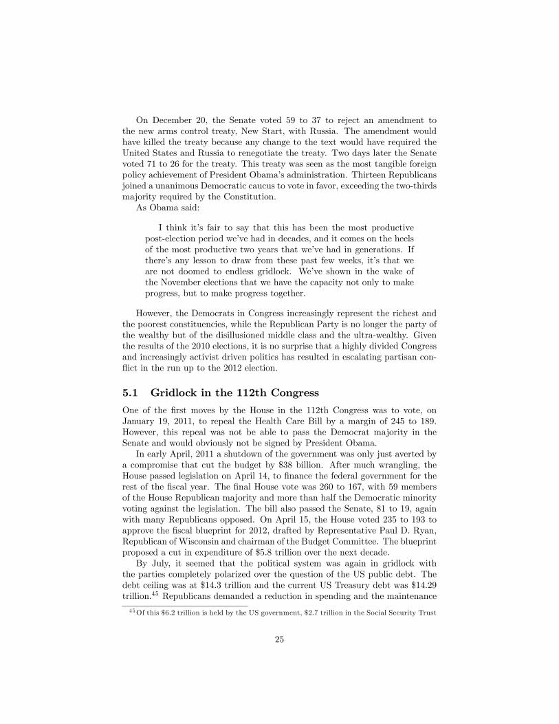
On December 20, the Senate voted 59 to 37 to reject an amendment tothe new arms control treaty, New Start, with Russia. The amendment wouldhave killed the treaty because any change to the text would have required theUnited States and Russia to renegotiate the treaty. Two days later the Senatevoted 71 to 26 for the treaty. This treaty was seen as the most tangible foreignpolicy achievement of President Obama’s administration. Thirteen Republicansjoined a unanimous Democratic caucus to vote in favor, exceeding the two-thirdsmajority required by the Constitution.As Obama said:

I think it’s fair to say that this has been the most productivepost-election period we’ve had in decades, and it comes on the heelsof the most productive two years that we’ve had in generations. Ifthere’s any lesson to draw from these past few weeks, it’s that weare not doomed to endless gridlock. We’ve shown in the wake ofthe November elections that we have the capacity not only to makeprogress, but to make progress together.

However, the Democrats in Congress increasingly represent the richest andthe poorest constituencies, while the Republican Party is no longer the party ofthe wealthy but of the disillusioned middle class and the ultra-wealthy. Giventhe results of the 2010 elections, it is no surprise that a highly divided Congressand increasingly activist driven politics has resulted in escalating partisan con-flict in the run up to the 2012 election.

5.1 Gridlock in the 112th Congress

One of the first moves by the House in the 112th Congress was to vote, onJanuary 19, 2011, to repeal the Health Care Bill by a margin of 245 to 189.However, this repeal was not be able to pass the Democrat majority in theSenate and would obviously not be signed by President Obama.In early April, 2011 a shutdown of the government was only just averted by

a compromise that cut the budget by $38 billion. After much wrangling, theHouse passed legislation on April 14, to finance the federal government for therest of the fiscal year. The final House vote was 260 to 167, with 59 membersof the House Republican majority and more than half the Democratic minorityvoting against the legislation. The bill also passed the Senate, 81 to 19, againwith many Republicans opposed. On April 15, the House voted 235 to 193 toapprove the fiscal blueprint for 2012, drafted by Representative Paul D. Ryan,Republican of Wisconsin and chairman of the Budget Committee. The blueprintproposed a cut in expenditure of $5.8 trillion over the next decade.By July, it seemed that the political system was again in gridlock with

the parties completely polarized over the question of the US public debt. Thedebt ceiling was at $14.3 trillion and the current US Treasury debt was $14.29trillion.45 Republicans demanded a reduction in spending and the maintenance

45Of this $6.2 trillion is held by the US government, $2.7 trillion in the Social Security Trust

25

of tax cuts, while Democrats basically wanted the opposite, continued spendingon social programs and tax increases on certain segments of the population.The House on Friday July 29, finally approved a plan for a short-term in-

crease in the debt ceiling and cuts in spending. The vote was 218-210, with22 Republicans unwilling to support the efforts by House Speaker, John A.Boehner, to get a bill approved. This ended a week of intense fighting amongRepublicans. The game then shifted to the Senate which tabled the House pro-posal. On August 1 the House of Representatives passed a compromise bill,269-161, supported by Democrats, increasing the debt ceiling by $400 billion,with an additional $500 billion through February, with spending caps of over$900 billion. A newly designed joint committee was vested with the responsi-bility of determining future cuts of over $1 trillion. The Senate passed the bill74-26 on August 2 with 19 Republicans, and 6 Democrats and one independentvoting against. President Obama immediately signed the bill into law. De-spite the eventual compromise on the debt ceiling, on August 5, 2011 Standardand Poor, the credit rating agency, downgraded US Federal debt from AAA toAA+, and the Dow industrial index dropped about 20% in the following days.However, demand for U.S. Treasury Bonds increased.On September 13, President Obama acted on the economic turmoil set off by

the Debt Ceiling debate, Standard and Poor downgrade and continuing Euro-pean debt crisis by sending a $447 billion jobs bill to Congress. Initial reactionfrom Republicans indicated a willingness to accept some measures of the bill,coupled with an insistence on keeping tax cuts for the wealthiest and resistenceto closing corporate loopholes. On November 21, however, the Joint Committeeto reduce the deficit announced that it could not come to any agreement, butdeclared: “We remain hopeful that Congress can build on this committee’s workand can find a way to tackle this issue in a way that works for the Americanpeople and our economy.”The Dow closed down about 2% for the day.The debate over the jobs bill highlights the fact that, despite media atten-

tion to the contrary, Obama has attempted to attract and retain pro-businesssocial liberals with his response to the economic crisis. In addition to namingGeneral Electric CEO Jeffrey Immelt as Chairman of the President’s Councilon Jobs and Competitiveness, the President’s second Chief of staff was formerCommerce secretary and bank executive William Daley. These steps, along withhis massive budget proposals providing relief to banks and other businesses inorder to address the economic down-turn, has angered many in populist cir-cles. Meanwhile, insistence on closing corporate tax loopholes and the spectreof increased financial regulation, has eroded business support for the President.This lack of support in both the populist and cosmopolitan quadrants leaves

the President and his party vulnerable to attacks by traditionally conservativeRepublicans as well as to the more populist demands of the Tea Party. Asa result of persistently high unemployment rates, populist anger has spikedand it is and even spawned a second, distinctly liberal-minded populist group,

Fund, $1.9 trillion in other government agencies and $1.6 trillion in the Federal Reserve. Chinaand Hong Kong hold $1.3 trillion, other countries hold $3.2 trillion, the remaining $3.6 trillionis held by pension funds etc.

26

the "Occupy Wall Street" protesters. It is possible that the Republican Partywill gain votes from the blue-collar voters who are suffering the most from theeconomic collapse. Should the Republican party cater to the traditional populistdemands expressed by those in the Tea Party, they will be hearkening back toan era of old-style populism as expressed by William Jennings Bryan: anti-Wall Street, anti-banking, anti-Detroit, anti-immigration, and pro-evangelicalreligion. This will result in a party realignment to a situation where the sociallyliberal and economically conservative “cosmopolitan”Democrats are opposedto populist Republicans.That is, the Republican Party may begin to move tothe lower left quadrant of the policy space, while some business interests in theupper right quadrant will switch to the Democrats.46 Over the long term, thepartisan cleavage line may rotate further in a clockwise direction.

6 Conclusion and 2012

Money has made US politics irrational. With legal barriers falling and moneyplaying an increasingly large role in recent elections, this irrationality and non-convergence to the electoral center is likely to persist. The 2012 election cyclehighlights the role of money and non-convergence. Early Republican Presiden-tial frontrunners included Tea Party darlings Representative Michele Bachman,Representative Ron Paul, and Governor Rick Perry along with seasoned con-servative ideologues former Senator Rick Santorum and former Speaker of theHouse Newt Gingrich. Comparing himself to the other Republican candidates,Former Governor Mitt Romney initially admitted to seeking a more centristroute to the nomination, but facing activist money such as the PAC "Make UsGreat Again" which supported Rick Perry to the tune of $55 million and billion-aire Sheldon Adelson who provided tens of millions in support of Newt Gingrich,Romney was forced to adopt increasingly conservative policy positions. By theend of the primary campaign, some Repulican strategists were publicly declaringconcern that Governor Romney had taken such radically conservative positionsin the primaries that it might be hard for him to appeal to moderate voters inthe general election. All the while, new legal precedent allowed the Federal Elec-tion Commission to turn a blind eye to the creation of candidate Super PACs,such as “Make Us Great Again” for Republican Rick Perry and “Restore OurFuture”for Republican Mitt Romney. Even President Obama’s PAC “PrioritiesUSA”plans to raise $100 million for the 2012 election.Utilizing the model we have presented, we contrast the current situation with

the 1960s. After Kennedy was elected President in 1960 (by a very narrow mar-gin of victory against Nixon), he delayed sending a Civil Rights Bill to Congress,precisely because of the possible effect on the South (Branch, 1998). To pushthe Civil Rights Act through in 1964, Johnson effectively created, with HubertHumphrey’s support, an unstable coalition of liberal northern Democrats andmoderate Republicans, with suffi cient votes in the Senate to effect ‘cloture’, to

46For example, on April 28, 2010 Arlen Specter, the Senator from Pennsylvania, shifted hisallegiance from the Republican Party to the Democrats.

27

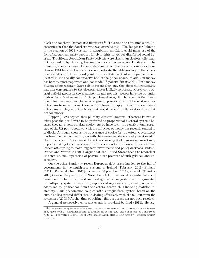
block the southern Democratic filibusters.47 This was the first time since Re-construction that the Southern veto was overwhelmed. The danger for Johnsonin the election of 1964 was that a Republican candidate could make use of thefact of Republican party support for civil rights to attract disaffected social lib-erals. Traditional Republican Party activists were thus in an electoral dilemma,but resolved it by choosing the southern social conservative, Goldwater. Thepresent gridlock between the legislative and executive branchs is more extremethan in 1964 because there are now no moderate Republicans to join the social-liberal coalition. The electoral pivot line has rotated so that all Republicans arelocated in the socially conservative half of the policy space. In addition moneyhas become more important and has made US politics "irrational". With moneyplaying an increasingly large role in recent elections, this electoral irrationalityand non-convergence to the electoral center is likely to persist. Moreover, pow-erful activist groups in the cosmopolitan and populist sectors have the potentialto draw in politicians and shift the partisan cleavage line between parties. Wereit not for the resources the activist groups provide it would be irrational forpoliticians to move toward these activist bases . Simply put, activists influencepoliticians so they adopt policies that would be electorally irrational, were itnot for money.Popper (1988) argued that plurality electoral systems, otherwise known as

“first past the post”were to be preferred to proportional electoral systems be-cause they gave voters a clear choice. As we have seen, the constitutional struc-ture of the US polity, coupled with the influence of money has recently tended togridlock. Although there is the appearance of choice for the voters, Governmenthas been unable to come to grips with the severe quandaries briefly mentioned inthe introduction. The absence of effective choice by the US increases uncertaintyin policymaking thus creating a diffi cult situation for business and internationalleaders attempting to make long-term investments and policy decisions. Indeed,Posner and Vermeule (2011) argue that the United States needs to reconsiderits constitutional separation of powers in the presence of such gridlock and un-certainty.On the other hand, the recent European debt crisis has led to the fall of

governments in the multiparty systems of Ireland (February, 2011) Finland(2011), Portugal (June 2011), Denmark (September, 2011), Slovakia (October2011),Greece, Italy and Spain (November 2011). The model presented here anddeveloped further in Schofield and Gallego (2012) suggests that in fragmentedor multiparty systems, based on proportional representation, small parties willadopt radical policies far from the electoral center, thus inducing coalition in-stability. This phenomenon coupled with a fragile fiscal system based on theeuro also has created diffi culties in dealing effectively with the fall-out from therecession of 2008-9.At the time of writing. this euro crisis has not been resolved.A general perspective on recent events is provided by Lind (2012). He sug-

47Caro (2012: 568) describes the drama of the cloture vote of Jun 10, 1964 after a filibusterof 57 days with 27 Republicans and 44 Democrats voting aye. The bill passed on June 19 by73 to 27. The voting Rights Act of 1965 passed again after a long fight by Johnston againstCongress.

28

gests that in order to maintain a post World War II international economicsystem to facilitate growth and oppose the Soviet Union the US maintained itshegemonic power by its willingness to accept mercantilistic trade strategies byits allies Germany, Japan. In the first 30 years until the oil crisis of the 1970’sthis system could be maintained without great cost. Indeed economic grpwthin the US was maintained. Although Nixon tried to limit this mercantilism bycoming of the gold standard in 1973, Finance capital exerted pressure to sus-tain this systm of US dominance. After the fall of the Soviet Union, it seemedattractive to allow China to institute trade mercantilism, allowing it to growvery rapidly. As Keynes saw back in 1945, such a system is inherently unstable.The resulting "globalization"( and increased trade flows) has led to the massiveUS trade deficits of the last thirty or forty years, and the loss of much of themanufacturing capacity of the US. While increased trade has contibuted to anincrease in global GDP,it has forced down unskilled wage rates in the US. It is forthis reason that the US has become such an unequal economy (Stiglitz, 2012),making the conflict between labor and capital more intense.. High artificial sav-ings by China and its willingness to fund US debt (both necessary componentsof its mercantilism) disguised the costs to the US, but also provided the financialbasis for the extreme form of speculation that came to dominate the market.Capital benefitted from globalization. and was able to fund political support forthe maintenance of this hegemonic system. Stiglitz adds that the current modeof oligopoly rent seeking in the US is consistent with with the external patternof hegemony and sustains both inequality and underprovision of social publicgoods such as innovation. Since the most important global public good is pre-vention of climate change, the severe costs of this potentally unstable politicaleconomic system will burden future generations.48

48 Israel (2012) has pointed out that the modern period since 1700 witnessed a conflict be-tween a Radical Enlightenment espoused by Condorcet, Jefferson and Paine, in support ofreason and equality and opposed to monarchy and hierarchical hegemony, and the compro-mising Moderate Enlightenment of Hamilton and Burke.

29

6.0.1 Acknowledgement

This paper is based on work supported by NSF grant #0715929

References

[1] Abramowitz, A. (2010) The Disappearing Center. New Haven: Yale Uni-versity Press.

[2] Abramowitz, A. Saunders A.. (2005) ’Why Can’t We Get Along: TheReality of Polarized America.’Forum 3 (2) Article 1:1-21.

[3] Adams, J. (2001) Party Competition and Responsible Party Government.Ann Arbor: University of Michigan Press.

[4] Acemoglu, D., and J. Robinson. (2008). ‘Persistence of Power, Elites, andInstitutions.‘American Economic Review 98, 267-293.

[5] Aldrich, J. H. (1983). ’A Downsian Spatial Model with Party Activists.’American Political Science Review, 77 (4), 974—90.

[6] Allen, F.L. (1994) Since Yesterday: The 1930’s in America. New York:Borgo.

[7] Alpert, D., Hockett, R. and N. Roubini, N. (2011). The Way Forward.The New America Foundation. (www.newamerica.net).

[8] American national election studies. 2004, 2008.

[9] Ansolabehere, S., Rodden, J. and Snyder, J. Jr. (2006). ’Purple America.’Journal of Economic Perspectives, 20, 97-118.

[10] Aragones, E. and Palfrey, T. (2002). ’Mixed Equilibrium in a DownsianModel with a Favored Candidate,’ Journal of Economic Theory, 103,131—61.

[11] Ashworth, S. and Bueno de Mesquita, E. (2009). ’Elections with Platformand Valence Competition.’ Games and Economic Behavior, 67, 191—216.

[12] Banks J. and Duggan, J. (2005). ’Probabilistic Voting in the Spatial Modelof Elections: The Theory of Offi ce Motivated Candidates’, in D. Austen-Smith and J. Duggan (eds), Social Choice and Strategic Decisions: Essaysin Honor of Jeffrey Banks. Heidelberg: Springer.

[13] Branch, T. (1998). Pillar of Fire. New York: Simon and Schuster.

[14] Buchanan, P. (2011).Suicide of a Superpower. new York: St.Matins Press.

[15] Buchanan, P. (1998). The Great Betrayal: How American Sovereignty andSocial Justice are Being Sacrificed to the Gods of the Global Economy. NewYork: Little Brown.

30

[16] Bunch, W. (2010). Backlash. New York: Harper.

[17] Calvert, R. L. (1985). ’Robustness of the Multidimensional Voting Model:Candidates, Motivations, Uncertainty and Convergence’, American Jour-nal of Political Science 29, 69—85.

[18] Caro (2012) The Passage of Power. New York. Knopf.

[19] Chace, J. (2004). 1912: Wilson, Roosevelt, Taft and Debs. New York:Simon and Schuster.

[20] Clarke H.D., A.Kornberg A. and T. J. Scotto. (2009). Making PoliticalChoices. Toronto: Toronto University Press.

[21] Clarke, H, D., Kornberg A., Scotto, T., Reifler, J., Sanders, D., StewartM. and Whiteley, P. (2011). “Yes We Can! Valence politics and electoralchoice in America 2008’, Electoral Studies 30, 450-461.

[22] Clinton, W. (2011). Back to Work. New York: Knopf

[23] Coate, S. (2004) ’Political Competition with Campaign Contributions andInformative Advertising.’ Journal of the European Economic Association,2, 772-804.

[24] Crick (1995). The Astonishing Hypothesis. New York, Scribner.

[25] Dawkins, R. (2011) The Magic of Reality New York: Free Press.

[26] Downs, A. (1957) An Economic Theory of Democracy. New York: Harperand Row.

[27] Duggan, J. (2006). ’Candidate Objectives and Electoral Equilibrium’, inB.R.Weingast, D. Wittman (eds) The Oxford Handbook of Political Econ-omy. Oxford: Oxford University Press.

[28] Duggan, J. and Fey, M. (2005). ’Electoral Competition with Policy-Motivated Candidates’, Games and Economic Behavior, 51, 490-522.

[29] Enelow, J.M. and Hinich M. (1989). “The Location of American Presi-dential Candidates”, Mathematical Computer Modelling, 12, 417-35.

[30] Erikson, R.S. and D.W. Romero D.W.. (1990) ’Candidate Equilibrium andthe Behavioral Model of the Vote’, American Political Science Review, 84,1103-126.

[31] Field, A.J. (2003). ’The Most Technologically Progressive Decade of theCentury. American Economic Review 93, 1399-1414.

[32] Fisher, I. (1933). ’The Debt-Deflation Theory of Great Depressions.’Econometrica, 1:337-357.

31

[33] Fiorina M., Abrams, S.J. and Pope, J.C. (2005) Culture War?: The Mythof a Polarized America. New York: Pearson Longman.

[34] Fiorina M. and Abrams, S.J. (2009) Disconnect: The Breakdown of Rep-resentation in American Politics. Norman, OK:University of OklahomaPress

[35] Friedman T. and Mandelbaum M. (2011) That Used to be Us. New York:Farrar, Straus and Giroux.

[36] Galbraith J.K. (2008) The Predator State. New York: Free Press.

[37] Gelman, A. (2009) Red State, Blue State. Rich State, Poor State. Prince-ton NJ: Princeton University Press.

[38] Gould, L.L. 2008). Four Hats in the Ring. Lawrence KS: University ofKansas Press.

[39] Graham, J., Haidt, J. and Nosek, B. 2009. ’Liberals and Conservatives relyon Different Moral Foundations.’Jour of Personality Social Psychology,96, 1029-046.

[40] Groseclose, T. and Snyder, J. (1996) ’Buying Supermajorities,’AmericanJournal of Political Science, 90, 303-15.

[41] Grossman, G. M. and Helpman, E. (1994) ’Protection for Sale’, AmericanEconomic Review, 84, 833-50.

[42] Grossman, G. M., and Helpman, E. (1996_. ’Electoral Competition andSpecial Interest Politics’, The Review of Economic Studies, 63, 265-86.

[43] Grossman, G. M. and Helpman, E. (2001) Special Interest Groups. Cam-bridge, MA: MIT Press.

[44] Hacker, J.S. and Pierson, P. (2006) Off Center: The Republican Revolutionand the Erosion of American Democracy. New Haven CT: Yale UniversityPress.

[45] Hitchens, C (2007). God Is Not Great. New York: Twelve.

[46] Hacker, J.S. and Pierson, P. (2010)Winner-Take-All Politics: How Wash-ington Made the Rich Richer—and Turned Its Back on the Middle Class.New York: Simon and Schuster.

[47] Harvey, D. (2011). The Enigma of Capital and the Crises of Capitalism.Oxford: Oxford University Press.

[48] Herrera H., Levine D. and Martinelli C. (2008) ’Policy platforms, Cam-paign Spending and Voter Participation.’Journal of Public Economics,92, 501-13

32

[49] Hotelling, H. (1929). ’Stability in Competition.’ Economic Journal,39,41—57.

[50] Israel, J. (2012) Democratic Enlightenment. Oxford: Oxford UniversityPress.

[51] Keynes, J. M. 1930a) A Treatise on Money. Vol. 1: The Pure Theory ofMoney. Reprinted inKeynes, Collected Writings. Vol. 5. London: Macmil-lan.

[52] Keynes, J. M.. 1930b. A Treatise on Money. Vol. 2: The Applied The-ory of Money. Reprinted in Keynes, Collected Writings. Vol. 6. London:Macmillan.

[53] Keynes, J. M.. 1933. ’National Self-Suffi ciency.’Yale Review 26: 755—69.

[54] Keynes, J. M. (1936). The General Theory of Employment, Interest andMoney. London: Macmillan.

[55] Kramnick, I. (1990). Republicanism and Bourgeois Radicalism. Itahca,NY: Cornell University Press. University Press.

[56] Kramnick, I. (1992.[1968]). Bolingbroke and his Circle. Ithaca, NY: Cor-nell University Press.

[57] Krugman (2012) End This Deprtession Now ! New York: Norton

[58] Krasa, S.and Polborn M. (2011) ’The Relative Importance of Culturaland Economic Issues for the Polarization of the US Electorate, 1972-2008.’Working Paper: University of Illinois.

[59] Layman, G.C. et al. (2010) ’Party Polarization, Party Commitment andConflict Extension among American Party Activists.’American PoliticalScience Review, 104,324—346.

[60] Lessig, L. 2011. Republic, Lost. New York: Twelve.

[61] Livingstone, J. (2011). Against Thrift. New York: Basic.

[62] Lind M. (2012) Land of Promise. New York: Harper.

[63] Madison, J. (1999 [1787]) Federalist X, in Rakove J. (ed) Madison: Writ-ings. New York: Library Classics.

[64] McCarty N., Poole K. and Rosenthal H. (2006) Polarized America. Cam-bridge MA: MIT Press.

[65] McKelvey, R. D., Patty, J. (2006) ’A Theory of Voting in Large Elections.’Games and Economic Behavior. 57, 155—80.

[66] Meirowitz, A. (2008) ’Electoral Contests, Incumbency Advantages andCampaign Finance’, Journal of Politics 70 681-99.

33

[67] Milanovic, B. (2010) The Haves and the Have Nots. New York: Basic.

[68] Micklethwaite, J. and Wooldridge A. (2004) The Right Nation.New York:Penguin

[69] Miller G, Schofield N. (2003) ’Activists and partisan realignment in theU.S.’American Political Science Review 97, 245—260.

[70] Miller G, Schofield N. (2008) ’The Transformation of the Republican andDemocratic coalitions in the U.S.’Perspectives on Politics 6,433-450

[71] Minsky, H. (1986) Stabilizing an Unstable Economy. New Haven: YaleUniversity Press.

[72] Morgenson, G., Rosner, J. 2011. Reckless Endangerment. New York: Holt.

[73] Noah T. (2012). The Great Divergence. New York: Bloomington.

[74] Olson, M. 1982. The Rise and Decline of Nations. New Haven: Yale Uni-versity Press.

[75] Penn, E. (2009) ’A Model of Far-Sighted Voting’, American Journal ofPolitical Science, 53,36-54.

[76] Patty J., Snyder, J.M. and Ting, M. (2009) ’Two’s Company, Three’s AnEquilibrium: Strategic Voting and Multicandidate Elections’,QuarterlyJournal of Political Science. 4,251-78.

[77] Peress M. (2010) ’The Spatial Model with Non-Policy Factors: A Theoryof Policy Motivated Candidates’, Social Choice and Welfare, 34,265-94.

[78] Pierson, P. and Skocpol, T. [eds] (2007) The Transformation of AmericanPolitics: Activist Government and the Rise of Conservatism. Princeton,NJ: Princeton University Press.

[79] Poole, K. and Rosenthal, H. (1984) ’U.S. Presidential elections 1968-1980:A Spatial Analysis’, American Journal of Political Science, 28, 283—312.

[80] Popper, K. (1945) The Open Society and its Enemies. London: Routledgeand Kegan Paul.

[81] Popper, K. (2008) ’The Open Society and its Enemies Revisited’, TheEconomist 307, 19-22.

[82] Posner, E.A. and Vermeule A. (2011). The Executive Unbound. Oxford:Oxford University Press.

[83] Putnam , R.D. and Campbell D.E. (2010). American Grace: How ReligionDivides and Unites Us. New York: Simon and Schuster.

[84] Rachman, G. (2011). Zero-Sum Future. New York: Simon and Schuster.

34

[85] Rasmussen, S. and Schoen, D. (2010). Mad as Hell: How the Teaparty Movement is fundamentally Remaking our Two-Party System. NewYork:Harper.

[86] Reich, R. B. (2010). Aftershock: The Next Economy and America’s Fu-ture. New York: Knopf.

[87] Sachs, J.D. (2011). The Price of Civilization: Reawakening AmericanVirtue and Prosperity. New York: Random House.

[88] Sandel (2012) What Money Can’t Buy. New York: Ferrar, Strauss andGiroux.

[89] Sanders, D., Clarke, H.D., Stewart, M.C. and Whiteley, P. (2011). ’Downs,Stokes and the Dynamics of Electoral Choice. British Journal of PoliticalScience, 41, 287-314.

[90] Schofield N.(2006). Architects of Political Change:Constitutional Quan-daries and Social Choice Theory. Cambridge: Cambridge University press.

[91] Schofield N.(2007).The Mean Voter Theorem: Necessary and Suffi cientConditions for Convergent Equilibrium.”The Review of Economic Stud-ies, 74(3): 965-980.

[92] Schofield N. and M. Gallego (20012) Leadership or Chaos. Berlin:Springer.

[93] Schofield N., Miller G. (2007) ’Elections and Activist Coalitions in theU.S.’American Journal of Political Science 51, 518—531.

[94] Schofield N, Miller G, and Martin A (2003) ’Critical elections and politicalrealignments in the U.S.: 1860-2000.’Political Studies 51, 217—240.

[95] Schumpeter, J. 1942. Capitalism, Socialism, and Democracy. New York:Harper.

[96] Skocpol, T. and Williamson, V. (2010). The Tea Party and the Re Makingof Republican Conservatism. Oxford: Oxford: University Press.

[97] Smith (2012) Who Stole the American Dream? New York: RandomHouse.

[98] Steyn, M. (2011) After America. New York: Regnery.

[99] Stokes D. (1963) ’Spatial Models and Party Competition’, American Po-litical Science Review, 57,368—377.

[100] Stokes D. (1992) ’Valence Politics’, in D.Kavanagh (ed) Electoral Politics.Oxford: Clarendon Press .

[101] Stiglitz, J.E. (2012)The Price of Inequality: How Today’s Divided SocietyEndangers Our Future. New York: Norton

35

[102] Tomasky M. (2010) ’The Money Fighting Health Care Reform’, New YorkReview of Books, 57(6):10-14.

[103] Triffi n, R. (1960). Gold and Dollar Crisis. New Haven: Yale UniversityPress.

[104] Von Hayek, F. (2007.[1944]). The Road to Serfdom. Chicago: The Univer-sity of Chicago Press and London: Routledge & Kegan Paul.

[105] Von Mises, L. (1949 [1940]).Nationalökonomie: Theorie Des Handelnsund Wirtschaftens. Trans. as Human Action. New Haven: Yale UniversityPress.

[106] Wittman, D. (1977) ’Candidates with Policy Preferences: A DynamicModel’, Journal of Economic Theory 14,180-89.

36

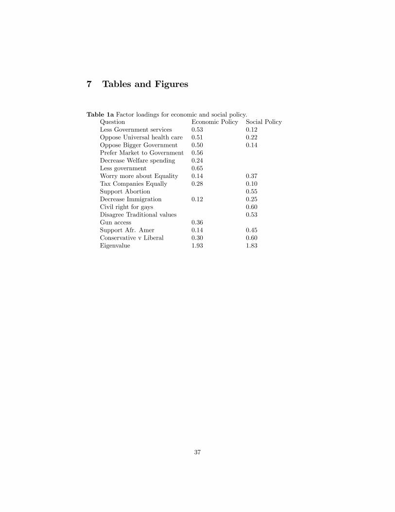
7 Tables and Figures

Table 1a Factor loadings for economic and social policy.Question Economic Policy Social PolicyLess Government services 0.53 0.12Oppose Universal health care 0.51 0.22Oppose Bigger Government 0.50 0.14Prefer Market to Government 0.56Decrease Welfare spending 0.24Less government 0.65Worry more about Equality 0.14 0.37Tax Companies Equally 0.28 0.10Support Abortion 0.55Decrease Immigration 0.12 0.25Civil right for gays 0.60Disagree Traditional values 0.53Gun access 0.36Support Afr. Amer 0.14 0.45Conservative v Liberal 0.30 0.60Eigenvalue 1.93 1.83

37

Table 1b Descriptive data for the 2008 Presidential ElectionEcon Policy Social Policy nMean s.e. 95% C.I Mean s.e 95% C.I

ActivistsDemocrats -0.20 0.09 [-0.38, -0.02] 1.14 0.11 [0.92,1.37] 80Republicans 1.41 0.13 [1.66, 1.16] -0.82 0.09 [-0.99,-0.65] 40

Non-activistsDemocrats -0.17 0.03 [-0.24,-0.11] 0.36 0.04 [0.29,0.44] 449Republicans 0.72 0.06 [0.60,0.84] -0.56 0.05 [-0.65,-0.46] 219

788

Table 2. Obama and McCain electorally perceived positionsQuestion Obama McCainEstimated position on economic policy -0.22 0.59Estimated position on social policy 0.75 -0.37

Table 3 Factor loadings for candidate traits scores 2008Question Obama Traits McCain TraitsObama Moral .72 -.01Obama Caring .71 -.18Obama Knowledgeable .61 -.07Obama Strong .69 -.13Obama Honest .68 -.09Obama Intelligent .61 .08Obama Optimistic .55 .00McCain Moral -.09 .67McCain Cares -.17 .63McCain Knowledgeable -.02 .65McCain Strong -.10 .70McCain Honest -.03 .63McCain Intelligent .11 .68McCain Optimistic -.07 .57Eigenvalue 3.07 3.00

38

Table 4. Spatial Logit Models for USA 2008a

Variable (1) Spatial (2) Sp. & Traits (3) Sp. & Dem. (4) FullMcCain valence λ −0.84∗∗∗ −1.08∗∗∗ −2.60∗∗ −3.58∗∗∗

(7.6) (8.3) (2.8) (3.4)Spatial β 0.85∗∗∗ 0.78∗∗∗ 0.86∗∗∗ 0.83∗∗∗

(14.1) (10.1) (12.3) (10.3)McCain traits 1.30∗∗∗ 1.36∗∗∗

(7.6) (7.15)Obama traits −1.02∗∗∗ −1.16∗∗∗

(6.8) (6.44)Age -0.01 -0.01

(1.0) (1.0)Gender (F) 0.29 0.44

(1.26) (0.26)African American −4.16∗∗∗ −3.79∗∗∗

(3.78) (3.08)Hispanic -0.55 -0.23

(1.34) (0.51)Education 0.15∗ 0.22∗∗∗

(2.5) (3.66)Income 0.03 0.01

(1.5) (0.50)Working Class −0.54∗ −0.70∗∗

(2.25) (2.59)South 0.36 -0.02

(1.5) (0.07)Observations 788log likelihood (LL) -299 -243 -250 -207AIC 601 494 521 438BIC 611 513 567 494

* prob < 0.05, ** prob < 0.01,*** prob < 0.001.a Baseline Obama

39

­2 ­1 0 1 2

­2

­1

0

1

2

Economic Policy

Soc

ial P

olic

y

Bush

Kerry

median

Democrats

Republic ans

Figure 1: Electoral distribution and candidate positions in the United States in2004

­1.0 ­0.5 0.0 0.5 1.0

­1.0

­0.5

0.0

0.5

1.0

Economic  Policy

Socia

l Pol

icy

Figure 2: Comparison of mean partisan and activist positions for Democrat andRepublican voters in 2004 (error bars are larger for the mean activist positions.

40

x

x

x

x

x

x

x

x

x

x

x

x

x

x x

x

x

x

x

x

x

x

x xx

x x

x

x

x

x

x

x

x

x

x

x

x

x

x

xxx

x

x

x

x

x

x

x

xx x

x

x

x

x

x

x

x

x

x

x

x

x

x

x

x

x

x

x

x

x

x

x

x

x

x

x

xx

x

x

x x

x

x

x

x

x

x

x

x

x

x

x

x

xx

x

x

x

x x

x

x

x

x

x

x

x

x x

x

x

x

x

x x

x

xx

x

xx

x

x

x

x

x

x

x

x

x

x

x

x

x

xx

x

x

x

x

x

xx

x

x

x

x

x

x

x

x

x

x

x

x

xx

x

x

xx

x

x

x

x

x

x

x

x

x

x

x

x

x

x

x

x

xx

x

x

x

x

x

x

x

x x

x

xx

xx

x

x

x

x

x

xx

x

x xx

x

x

x

x

x

x

x

x

x x

x

x

x

x

x

xxx

x

x

x

x

x

x

x

x

x

x x

x

xx

x

x

x

x

xx

x

x

x

x

x x

x

x x

x

x

x

x

x

x

x

x

x

x

x

x

x

x

x

x

x

x

x

x

x

x

x

x

x

xx

x

x

x

x

x

x

x

xx

xx

x

x

x

xx

x

x

x

xx

x

x

x

x x

x

x

xxx

xx

x

x

x

x

x

xx

x

xx

x

x

x

x

x

x

x

xx

x

x

x

x

x

x

x

x

x

xx

x

x x

x

xx

x

xx

x

xx

x

x

xx

x

x

x

x

x x

x

x

x

x

xxx

x

x

x

x

xx

x

x

x

x

xxx

x

x

x

x

x

xx

xxx

x

x

x

x

x

x

x

xx

x

xx

x

x

xx

x

x

x

x

xx x

x

x

x

x

x

x

x

x

x

x

x

x

x

x

xx

x

xx

x

x

x

x

x

x

x

x

x

x

x

x

x

x

xx

x

x x

x

x

x

x

x

x

xxx

x

x

x

x

xxx

xx

x

x

x

xx

x

x

xx

x

x

xx

x

xx

x

x

x

x

x

x

x

x

x

x

x

x

x

x

x

x

xx

x

x

x

x

x

x

x

x

x

xx

x xx

x

xx

x

x x

x

xx

x

x

x

x

x

x

x

xx

x

x

x

x

x

x

x

x

x

x

x

x

x

x

x

x

xx

x

x

x

x

x

x

x

x

x

xx

xx

x

x

x

x

x

xx

x

x

x

x

x

x

x

xx

x

x

xx

x

x

xx

x

x

x

x

xx

x

x x

xx

x

x

x

x

x

x

xx

xx

x

xx

x

xx

x

x

xx

x

x

xx

xx

x

x

xx

x

x x

x

xx

x

x

x

xx x

x

xx

x

x

x

x

x

x

x

x

x

x

x

x

x

x

x x

x

x

x

xx

xx

x

x

x

x

x x

x

x

x

x

x

x

x

x

x

x

x

x

x

x

x

x

x

x

x

x x

x

x

x

x

x

x

xxx

x

x

x

x

x

x x

xx

x

x

x

x

xx

x

x

x

x

x

x

x

x

x

x

x

xx

x

x

xx

x

x

x

x

x

xx

x

x

x

x

x

x

x

x

x

x

x

xx

x

x

x

x

x

x

xx

x

x

x

x

x

x

x

x

x

­2 ­1 0 1 2

­2­1

01

23

Economic P olicy

Soc

ial P

olic

y

Obama

McCain

Figure 3: Distribution of voter ideal points and candidate position in 2008

xx

xx x

x

x x

x

xx

x

xx

x

x

x

x

x

x

xx

x

x

x

x

x

x

xx

x

x

x

xx

x

x

x

x

x

x

x

x

x

x

x

x xx

x

x

x

x

x

x

x

x

x

x

x

x

x

x

x

x x

x

x x

x

xx

x

x

x

x

x

­2 ­1 0 1 2

­2­1

01

23

Economic P olicy

Soc

ial P

olic

y

o

oo

oo

o

o

o

oo

o oo

o

o

o

oo

o

o

oo

ooo

o

oo

o

o

o

oo

oo

o

oo

o

Obama

McCain

x: Democr at Activistso: Repub lican Activists

Figure 4: Distribution of activist ideal points and candidate positions in 2008

41

Figure 5: Optimal Republican position

42

1

Sub-central governments and sovereign debt crisis in Spain over the period 2000-2011

Fernando Toboso (*) University of Valencia

I. Introduction

Since the financial crisis erupted in the fall of 2008, the government borrowing sector

has been in turmoil in almost all western developed countries. The present chapter

focuses on the quantitative evolution of sub-central, as well as central, government

borrowing in Spain, a country that is being experiencing serious problems at this

respect. Because an intense process of political and fiscal decentralization has taken

place in Spain since the mid eighties, the chapter examines whether this drive to

decentralization has been paralleled by any fiscally undisciplined behavior on the part of

sub-central governments over the periods 2000-2007 and 2008-2011. The empirical

analysis will be based on the internationally comparable public finance provided by the

OECD, the Eurostat and the Bank of Spain. As regards the breakdown by governmental

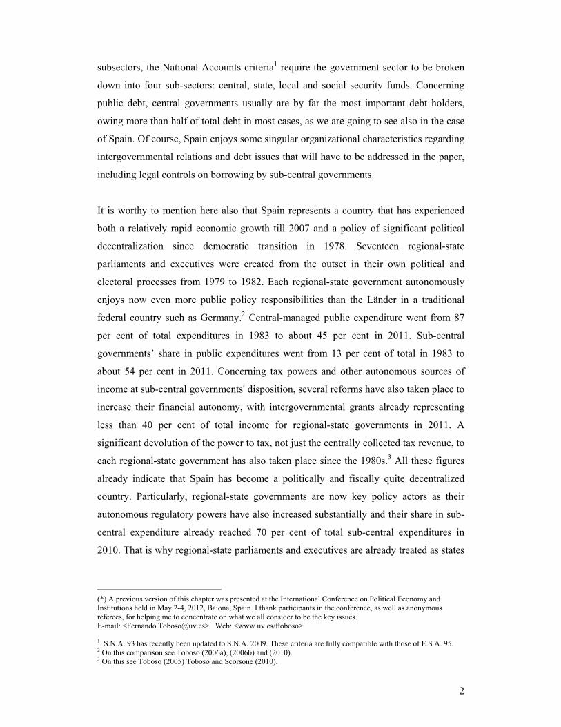
2

subsectors, the National Accounts criteria1 require the government sector to be broken

down into four sub-sectors: central, state, local and social security funds. Concerning

public debt, central governments usually are by far the most important debt holders,

owing more than half of total debt in most cases, as we are going to see also in the case

of Spain. Of course, Spain enjoys some singular organizational characteristics regarding

intergovernmental relations and debt issues that will have to be addressed in the paper,

including legal controls on borrowing by sub-central governments.

It is worthy to mention here also that Spain represents a country that has experienced

both a relatively rapid economic growth till 2007 and a policy of significant political

decentralization since democratic transition in 1978. Seventeen regional-state

parliaments and executives were created from the outset in their own political and

electoral processes from 1979 to 1982. Each regional-state government autonomously

enjoys now even more public policy responsibilities than the Länder in a traditional

federal country such as Germany.2 Central-managed public expenditure went from 87

per cent of total expenditures in 1983 to about 45 per cent in 2011. Sub-central

governments’ share in public expenditures went from 13 per cent of total in 1983 to

about 54 per cent in 2011. Concerning tax powers and other autonomous sources of

income at sub-central governments' disposition, several reforms have also taken place to

increase their financial autonomy, with intergovernmental grants already representing

less than 40 per cent of total income for regional-state governments in 2011. A

significant devolution of the power to tax, not just the centrally collected tax revenue, to

each regional-state government has also taken place since the 1980s.3 All these figures

already indicate that Spain has become a politically and fiscally quite decentralized

country. Particularly, regional-state governments are now key policy actors as their

autonomous regulatory powers have also increased substantially and their share in sub-

central expenditure already reached 70 per cent of total sub-central expenditures in

2010. That is why regional-state parliaments and executives are already treated as states

(*) A previous version of this chapter was presented at the International Conference on Political Economy and Institutions held in May 2-4, 2012, Baiona, Spain. I thank participants in the conference, as well as anonymous referees, for helping me to concentrate on what we all consider to be the key issues. E-mail: <Fernando.Toboso@uv.es> Web: <www.uv.es/ftoboso> 1 S.N.A. 93 has recently been updated to S.N.A. 2009. These criteria are fully compatible with those of E.S.A. 95. 2 On this comparison see Toboso (2006a), (2006b) and (2010). 3 On this see Toboso (2005) Toboso and Scorsone (2010).

3

are in federal countries, with their public finance figures being classified as such for the

reasons already mentioned.

Of course, all these figures represent a rough estimate of political decentralization

because they do not take into account many relevant qualitative aspects such us, for

example, the degree of discretion governments have regarding each type of expenditure,

or the exact degree of regulatory power each sub-central government enjoy. Some of

these expenditures may be financed from conditional grants or earmarked grants, for

example. But this is not an issue to be addressed in the present paper. The issue of how

are figures internally consolidated among subsectors will not be addressed either

because the impact of this aspect on global percentages is irrelevant for the research

purpose at hand.4 Local governments' public finances figures that will be used include

the spending, revenue, debt, etc by municipal and provincial governments, as well as by

other governmental agencies created by each municipality or related public enterprises,

as it is typically done when elaborating National Accounts statistics.5 The same

comments apply to the central and regional-state levels of government. In the case of

subsectors, debt issued by social security funds will appear included at the central level

as it is the central government who decides upon this debt in Spain.6. Figures referring

to “all governments” are consolidated among subsectors, as it is done in National

Accounts.

Therefore, to accomplish its purpose, the present chapter is organized as follows.

Following introductory remarks, in Section 1 I briefly review some of these key general

contributions to the topic being investigated in the present paper. In Section 2 an

empirical analysis is conducted for the period 1996-2007 on the Spanish case using

National Accounts multilevel public finance figures in order to show the evolution of

sub-central as well as central debt before the world financial crash. In this section the

paper emphasizes some singularities regarding key aspects of the multilevel

4 On these and other measuring problems see Martinez-Vezquez (2010), Toboso (2006) and Toboso and Scorsone (2010). 5 A different issue that will not be addressed in the paper is that in Spain as elsewhere there are several public services whose management has been externalized to private or public enterprises, to mixed consortiums, to public-private partnerships, etc. When these organizations belong to the business sector their activities are not directly accounted as part of the "general government" activities (central-regional-local-social security funds) but indirectly following National Account rules. 6 This is not the case regarding multilevel public finance statistics provided by the IMF. That is why the percentages that follow are not strictly comparable with IMF based percentages. The OECD databases do not provide desegregated figures for social security funds debt for all countries.

4

organization of government that exists in Spain, including legal details in place over the

period concerning the ability to incur in deficit and to issue debt by sub-central

governments. In Section 3 the same is done as regards to the 2008-2011 period that

followed the said financial crash. This section will show that Spain has experienced a

considerable increase in public deficit and debt since 2007, mainly at the central level. It

also points to the current economic recession and the initial counter-cyclical measures

adopted by all governments, including the increase in public expenditure needed for

bailouts in the financial sector, as key factors leading Spain to exceed during this second

period the limits on public deficit settled in the European Stability and Growth Path.

Section 4 concludes by emphasizing that economic conditions seem factors more

relevant for explaining the evolution of central and sub-central debt in Spain than

factors linked to political and fiscal decentralization arrangements. As stressed in

sections 3 and 4, the above statement is not to claim that debt limits, as well as some

other public sector regulatory details and behavioral political practices, are irrelevant.

The chapter also leaves for future econometric research the task of assigning numbers to

the relative magnitude in which each of these impact factors have influenced the

evolution of debt at the different tiers of government.

II. What are the main factors influencing the evolution of sub-central debt that are being emphasized in the literature?

Before examining what has happened with sub-central, as well as central, debt we need

briefly investigate which are the main factors influencing this evolution that are often

stressed in the literature. Rodden and others7 have made outstanding contributions on

these issues from a comparative institutional perspective. They have recurrently stressed

that institutional details characterizing federal systems are key factors (not necessarily

the only ones) for explaining differences in performance among federations. They

consider these factors crucial in explaining why sub-central governments behave in a

fiscally conservative manner in some countries while they rely on deficit financing in

others thus generating unsustainable levels of debt. This means that institutional-legal

arrangements, as well as informal social norms and values, matter in the economy as

well as in the polity. The key question however is: which institutional arrangements are

7 See Rodden (2002), Rodden and Wibbels (2002), Rodden et al. (2003), Rodden (2006).

5

decisive in each situation if political, economic and social circumstances as well as

participants differ so much from case to case? 8

Political and fiscal decentralization per se does not necessarily weaken fiscal discipline

of sub-central governments according to this strand of literature. A key aspect seems to

be whether the institutional setting for multilevel government provides expectations for

sub-central government leaders that there is a possibility to be bailed out, ceteris

paribus. In those multi-tiered systems of government in which the commitment by

central government to reject demands for bailout lack credibility, political agents at sub-

central governments may have the incentive to overspend and incur greater deficits if

they have unrestricted access to borrowing or borrowing limitations are not credibly

enforced.9

The incentive may be particularly relevant if political agents controlling a sub-central

government belong to a different political party or coalition than the party or coalition

controlling the central parliament and executive. The said incentive usually results in

strong efforts on the part of sub-central politicians to ensure re-election by finding local

and regional opportunities for spending if external financial sources are available and no

obligation to raising own taxes over regional constituents exists. This is also referred to

as the common pool problem.10 This bias may driven the behavior of all parties, lobby

groups and the people in general in the region or state. The more you get for “the state-

region” from the common pool, the better.

Using a sample of 43 countries over the period 1982-2000, Plekhanov and Singh (2006)

point to similar aspects as key factors in many cases. These authors conclude that no

single institutional arrangement seems superior under all circumstances for disciplining

sub-central government spending. Specific institutional characteristics of the country,

state or region, the existence of any bailout precedent, and the quality of fiscal reporting

seem relevant factors for all these countries.

8 See North (2005) or Ostron (1990) and (2005). 9 From a sample of 30 countries, Melo (2000) shows evidence indicating that intergovernmental fiscal relations are likely to result in a deficit bias in decentralized policy-making with soft budgets constrains. 10 Besley and Coate (2003), Knight (2006) and (2008), Inman and Rubinfel (1997), Baqir (2002), or Baron and Ferejohn (1987, 1989) address these common tax-pool issues mainly referring to the USA Congress and Senate. All emphasize on how the incentives created by national financing of local public goods lead to individual congressmen or senators to try to expand own-district spending at the same time that they try to restrain aggregate spending.

6

Among these arrangements, the effectiveness of debt and spending limits has received

considerable attention too in the literature, as well as the balanced budget rule. Studies

made upon panel data do not show a sole conclusion as usual. However, in many

occasions these limits seem to have lowered the spending rate of growth during the

boom periods, particularly if limits are well defined technically and it is easy to detect

non-compliance by independent management bodies. But this is not always the case, as

with regards to the US states for example, several authors have detected no significant

difference in expenditure or revenue growth between states with and without such

limitations for several periods of time. Shadbegian (1996) uses panel data from the

1960s till the1990s with such a conclusion. Kousser et al. (2008) investigates changes

within a given state, not among states, following the adoption of such ceilings and again

they find little impact over the subsequent years since.

Of course, sub-central governments with strict balanced budget rules or debt limits are

less able to help central government in the attempt to implement counter-cyclical

policies.11 Though, again, many exceptions and particularities exist from country to

country that have to be taken into account for an in depth analysis and sound

assessment. It must not be forgotten that debt limits typically apply only to guaranteed

debt, excluding debt issued by special public enterprises, as well as by some public

commercial agencies that are out of the so called "general government" entities whose

budgets are passed at all levels of government. Though this debt usually needs central

authorization, it represents a way to evade the said ceiling rules if central government

political leaders are likely to do so.

The consequences of economic cycles are also critical factors examined in the

literature.12 Recessions usually lead to deliberate countercyclical spending measures as

a first reaction.13 If we also consider impact on spending derived from the automatic

increase in other expenditures and the negative impact on tax revenues that also results,

there can be little doubt that recessions always produce a negative impact on public

11 See Levinson (1998), Fatás and Mihov (2006) and Rose (2006). 12 Barro (1979) is a seminal, much cited, contribution on this line of research. 13 Carlo (2009), for example, investigates the size and composition of the fiscal stimulus packages of the major economies that were implemented during 2008 in an attempt to cushion the decline on aggregate demand and growth that occurred as a result of the world financial crash.

7

deficits and debt levels. Bloechliger et al. (2010a) and (2010b) show that recessions

often affect public investment more than current expenditures as the former is easier to

curtail in the face of budget constraints, while current expenditures are politically more

sensitive or mandated and, consequently, more difficult to be changed.14 Poterba (1994),

for example, showed how the economic downturns in US during the late 1980s

significantly and negatively affected public deficits by the States. He also found that

political factors seemed were relevant, particularly for explaining deficits adjustments in

subsequent years. Adjustments were made faster when a single political party controls

the governorship and the state house than when party control was divided.15

Periods of economic growth just work on the opposite direction. On this line of research

and based on the evolution registered in the Swiss cantons between 1984 and 2000,

Freitag and Vatter (2008), for example, provide empirical results showing that in

periods of economic growth multilevel organization of government has no relevant

impact on debt. There are enough revenues for all governments to share. However, in

phases of economic recession differences among Cantons as regards to political

autonomy seem to affect the evolution of their debt. In these periods, suddenly spending

needs appear greater than public incomes and Cantons enjoying greater political

decentralization tend to implement more active budgetary policies than centralized

Swiss cantons, then incurring in greater debt.

There must be no doubt that both organizational factors as well as factors linked to

economic conditions are attracting the attention of scholars dealing with fiscal behavior

by sub central governments. However, knowing the relative role played by specific

formal and informal organizational details as compared to the role of the economic

cycle in determining the level and change in debt burdens is not an easy task. Moreover,

econometric exercises attempting to find the definitive factors that are valid are often

contradicted or refuted with other similar attempts found in the published literature. The

purpose of the present paper is quite different as indicated in the introductory section.

This paper attempts to quantitatively investigate the evolution of sub-central, as well as

central, public debt in Spain and see whether the turn in economic conditions is

14 See also Wibbels and Rodden (2006). 15 See also Allain-Dupré (2011).

8

paralleled by a similar turn regarding the evolution of debt. For accomplishing this

research purpose, the next section focuses on statistics for the 1996-2007 period.

III. The evolution of sub-central and central debt in Spain before the world financial crash.

As Spain experienced major changes in developing a new quasi-federal political system

from 1978 to 1983, it seems a suitable case study for investigating whether this political

and fiscal decentralization drive was paralleled by a negative evolution of public debt at

sub-central levels of government. How has public debt evolved in Spain? Did the world

financial crash and the sever recession initiated in 2008 cause any significant turning

point as regards to sub-central or central public debt?.

It is evident that public deficits and outstanding public debt were reduced at all levels of

government in Spain over the 2000-2007 period here considered if properly measured

as a percentage of GDP, as Table 1 reveals. Contrary to the case in some Latin-

American countries for example16, no relevant macroeconomic distortion has been

generated and no bailout problem has existed over the period. Moreover, Table 1 also

shows that both regional and local governments have contributed to the total

outstanding debt in very low proportion over the period. Roughly speaking, the central

government contributed about three times more than regional and local governments did

to outstanding debt. Since the mid 1990s, outstanding debt by the regional governments

has remained around 6 per cent of Spanish GDP and that one by local ones around 3 per

cent. Total outstanding debt in Spain has always been lower than the EU average level

over the period prior to the current financial crash, as Table 1 also indicates.

Table 1 General government debt in Spain

before the world financial crash broken down by levels (*) (% of GDP and Millions of Euros. National Accounts)

2000 2004 2006 2007Sub-central Governments 9.6 9.1 8.7 8.5

16 See Tanzi (2000) for an analysis of the potential macroeconomic problems. For an analysis of the bailout problem in the Argentina case, see Sanguinetti, J. y Tomassi, M. (2000, 2004), Tommasi, M., Saiegh, S. and Sanguinetti, P (2001) or Saiegh, Sebastian and Tommasi, Mariano (1999).

9

Regional Governments Local Governments

6.33.3

6.22.9

5.9 2.8

5.72.8

Central Government 51.5 37.1 31.0 27.7ALL GOVERNMENTS in Spain 61.1 46.2 39.7 36.1EU AVERAGE (Euro zone) 69.9 69.8 68.5 66.3Sub-central Govs Debt in Millions Euros Central Gov Debt in Millions Euros

59267314766

76148312994

86639 304416

90424291883

Sub-Central Govs Debt as % of Total Debt 15.84 19.56 22.15 23.65Source: OECD, Eurostat and Bank of Spain. Figures in the public domain. (*) All figures are made according to the European excessive-deficit protocol. Debt issued by Social Security Funds is included at the central level of government.

Graphically, this evolution of public debt broken down by levels of government can be

observed in Figure 1. If we take into consideration that over those years, the process of

political decentralization was very intense17, it can be stated that this political

decentralization was not paralleled by any relevant fiscal or debt problem at sub-central

or central levels of government. A different issue to be addressed in the next section is if

this new multilevel political system will be able to effectively respond to the fiscal

consolidation strategies required after the world financial crash.

Figure 1 General government debt in Spain

before the world financial crash broken down by levels (*) (% of the GDP and Millions of Euros. National Accounts)

17 Three years after the approval of the 1978 democratic Constitution, regional governments only managed 2.9 percent of total public expenditures. In 2006 they managed 33.1 percent. If we also take into account that total public expenditure in Spain has experienced a significant and rapid growth over those years (from 24.9 per cent of Spanish GDP in 1974 to about 40 percent on average over the 2000s.

10

Source: OECD, Eurostat and Bank of Spain. Figures in the public domain. (*) All figures are made according to the European excessive-deficit protocol. Debt issued by Social Security Funds is included at the central level of government.

Several explanations may help point towards what occurred in Spain during this period.

It is well-known that, along the past two decades, many developed countries have

significantly changed the context in which their fiscal policies operate, particularly by

adopting fiscal rules containing explicit limits to the public deficit and/or the

outstanding public debt. In some cases, explicit top ceiling to annual total expenditures

have also been settled. If compared with countries where these fiscal rules are absent or

not fully endorsed, the empirical evidence taken from the former ones tend to show

these rules as useful mechanisms in helping to maintain budgetary discipline, but

mainly during periods with enough economic growth.18 However, the specific design of

limitations and controls greatly determines the effectiveness of these rules. Monitoring

and enforcement aspects or the specific procedures settled for dealing with potential

deviations seem also crucial aspects.

Moreover, some central legal rules for borrowing have always existed since democratic

transition.19 Therefore, they may have played a role in maintaining the fiscal discipline

displayed by regional as well as by local governments over the period. However, these

legal rules have not been sufficient controls once the financial crash and its associated

18 See Debrun et al. (2008). 19 These Law initially passed in the central parliament were: Organic Law 8/1980 on Regional Governments Finances, Law 7/1985 and Law 38/1988 on local public finances. These laws have been reformed in several occasions since.

11

economic recession started. Thought an increase in public debt measured in millions

Euros was registered over the boom period, this did not cause any increase in the

relative percentage of sub central debt in terms of GDP, which is the most relevant

economic comparison. Controls and the economic cycle seemed to act to restrain

relative debt burdens across levels of government.

Though these rules and controls have also been changed on several occasions, a written

approval of the Central Finance Minister has always been required for regional

governments to access long term credit and issue debt, and specific constraints and

requirements were settled by Law for obtaining such a written authorization20. In

particular, for regional governments to get long term credit (longer than a year), two

requirement have always been in place. First, all credit must be dedicated to investment.

And second, annual repayment (capital and interests) must not be higher than 25% of

each regional government annual current income. As regarding the legal rules framing

financial sources at local governments’ disposition, two Laws were passed in the

Central Parliament since the very beginning of democratic transition, once the 1978

Constitution was in effect. These two initial legislation packages were Law 7/1985 and

Law 38/1988. The second is known as the Regulatory Law of Local Public Finances

(Ley Reguladora de las Haciendas Locales - LRHL). Several reforms have taken place

since those years.21 As a result of all these regulatory packages, local governments have

been subject to similar obligations in regards to budgetary stability as those affecting

regional governments, though some flexibility and exceptions are explicitly considered

in case of recessions in such legislative measures. Plans to progressively eliminate

public deficit deviations are also required. In all cases, authorizations to access credit

and issue short term and long term debt may be denied by the Central Finance Minister

if these plans are not fully implemented.22

20 In 2001, borrowing activities by Regional governments were also linked to the balanced budget principle, though some flexibility was introduced in the application of this principle in 2006, and latter on in 2009. 21 Two of these significant reforms regarding borrowing issues were implemented through Royal Decree 1463/2007 (which further develops basic principles settled in the General Law for Budgetary Stability already mentioned) and Royal Decree Law 5/2009 (which contained urgent and extraordinary measures to facilitate local governments to pay their providers if some obligations remained unpaid in 2008. Local government have had three months after the approval of teh 2009 Royal Decree Law for documenting these obligations that could not be paid and exceptionally apply for extra credit authorizations that will have to be repaid in six years maximum, that is in 2013). 22 An extra requirement exists for local governments to freely access short term credit (repaid along the year): the total amount obtained must not exceed 30 percent of current incomes in the previous year.

12

Moreover, it seems evident that the spectacular increase registered in total public

income on average over the growth period (both in total euros and as a percentage of

GDP), did also help in reducing public deficits and, consequently, the outstanding

public debt levels as shown in previous Table 1. An increasing amount of public income

has been available for financing public policies at all levels of government. Attention

must be paid to the fact that over this period, the Spanish GDP also grew significantly.

The economic growth registered over the period provided regional governments with an

increasing amount of financial resources. Most of this public income has come from the

increase registered in the Spanish tax revenue in relation to GDP: an increase of about

eighteen points in about thirty years (from 18.4 per cent of GDP in 1975 to 36.7 in 2006

according to the ministry of finance figures). Moreover, Spain has also been receiving,

until 2001, on average about 1-1.2 percent of GDP more each year in net terms as public

income from the European Union.23 The economic cycle seems a key issue as we are

going to emphasize in the next section. Therefore, the figures provided show that the

significant drive to political federalism and fiscal decentralization has not been

paralleled by a non-disciplined fiscal behavior on the part of sub-central governments

over the period that ended in 2007. Sub-central debt levels were reduced significantly in

total millions and in percentage of GDP, as OECD figures show. Sub-central public

deficit also went from -0.6 percent of GDP in 1996 to -0.4 in 2006.

IV. What has happened with sub-central, as well as, central debt in Spain after the world financial crash?

The above analysis does not mean that the singularities regarding political and fiscal

decentralization arrangements are irrelevant. However, after more than a decade leading

up to a major financial bubble in developed countries, some dramatic events erupted

around the fall of 2008. The severity of the economic recession generated and the initial

counter-cyclical measures adopted by all governments, together with some other

singular national factors, has lead to all European countries, in particular, to double or

triplicate the public deficit levels they registered prior to the financial crash, then

exceeding the limits established in the European Stability and Growth Pact (ESGP).

23 Since 2002, this source of income is becoming less significant in terms of GDP, and has suffered a further reduction for the period 2007-2014 as the twelve new countries that entered the EU in 2004 and 2007 are obtaining most of the EU funds for the new period.

13

Several other measures that are being taking necessarily imply more public spending as

is the case of the financial sector reform and those measures implemented to reorganize

and recapitalize banks and savings banks, with several banks already bailed-out.

In countries that were not able to significantly diminish public deficits and debt over the

boom, the consequences of recession, bankruptcies and bailouts in the financial sector,

to mention but a few events, have been more severe in terms of public deficit and debt.

This has caused considerable uncertainty on the part of international investors over the

ability of these governments to successfully issue new debt at reasonable interest rates

and even to pay back bonds previously issued.

But this evolution of debt levels alone does not explain why Spain has experienced such

a critical situation, particularly since the beginning of 2010. Japan, for example, has got

a debt burden of near 200 per cent of GDP and has had no similar financial problems at

international markets. Key issues in the case of Spain are the bad record regarding

economic growth since 2008, the bubble in the building sector that has finally burst and

seriously affected banks and saving banks, and also the many needs regarding current

and expected levels of elderly populations having the right to get a public pension. The

situation looks even worse if we consider the huge increase in unemployment that

Figure 2 shows. This reveals not only that internal demand has dropped and more and

more public expenditures are needed, but also that no dynamic export sector has come

as a substitute. As a result, a spectacular decrease in public revenue is taking place at all

tiers of government. Regarding the balance of payments, the current account external

trade deficit that Spain is registering, according to OECD figures (with no compensation

from the financial account) transmit the idea to international investor that problems will

not be solved in the near future. As higher is external debt (not just public external debt,

but also external debt by households, enterprises and banks) the worse regarding

expectations.

Figure 2 Unemployment in Spain

(Percentage of active population and number of people unemployed)

14

Source: Figures in the public domain from the Spanish National Institute of Statistics that are fully consistent with those provided by the OECD.

The importance of having or the lack thereof of effective fiscal rules and public deficit

and debt controls increases, of course, in the case of countries belonging to monetary

unions, as is the case of Spain. As the Euro zone case reveals since early 2010, the sharp

increase in public debt registered in some countries is clearly producing significant

negative impacts on other partners in the zone. This, in fact, was a main argument for

introducing the well-known public deficit and debt top limits into the European Union

Treaty at late 1980s. These shared consequences have also lead to the several

amendments of the already mentioned European Stability and Growth Pact (ESGP) that

have taken place. They have finally been used also for justifying interventions or

bailouts (Greece, Ireland, Portugal, and the bailout plan for the saving banks in Spain).

In all these countries, the extremely critical economic situation created since 2008,

together with the particularities of the specific economic problems affecting each

country, has resulted in spectacular increases in outstanding public debt levels in just

four years. In the case of Spain, the total public debt has doubled in terms of the Spanish

GDP if 2011 and 2007 years are compared, as Table 2 shows (from 36.1 per cent of

GDP to 72.1 per cent). Sub-central governments' debt has also experienced a significant

increase with about 68 thousand millions euros added to the stock of Spanish public

debt in just four years, with regional governments as main contributors. However it has

been at the central level of government where the drastic turning point in economic

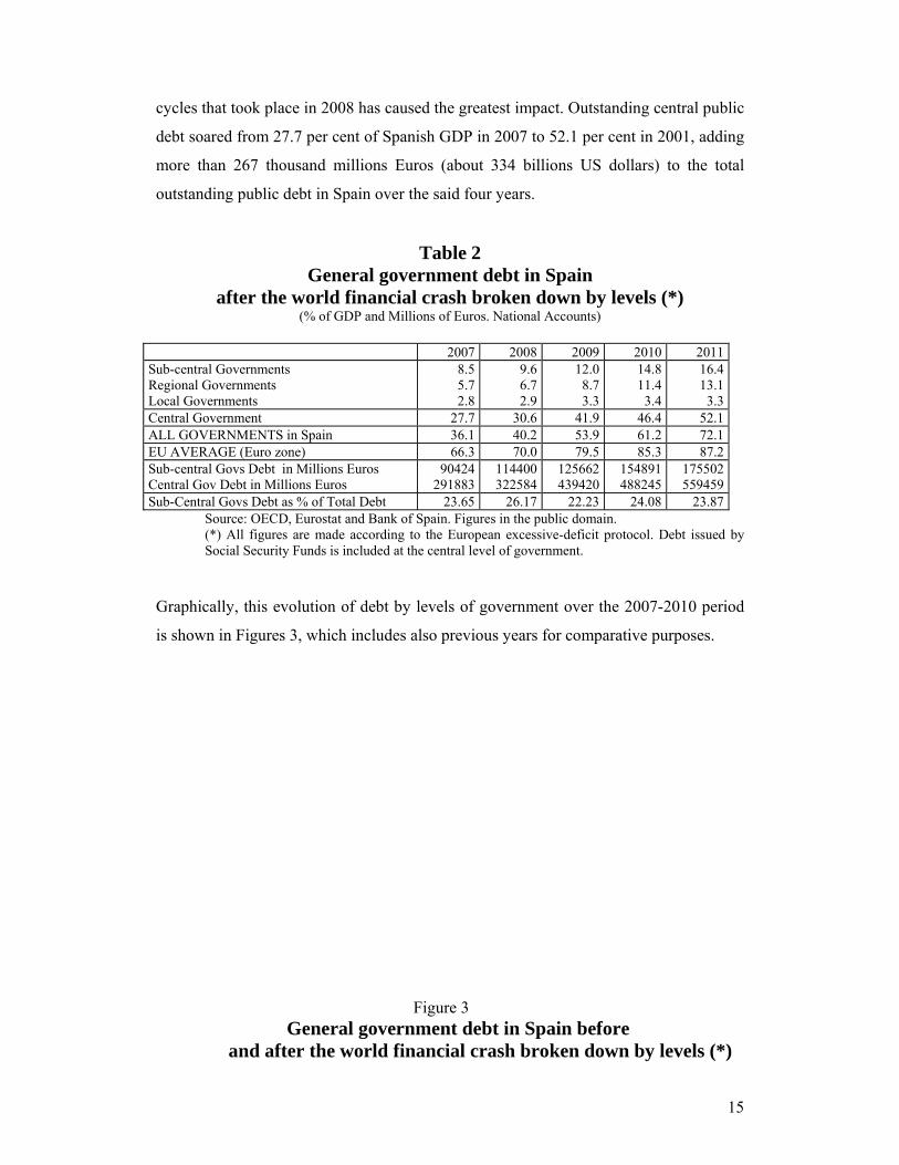
15

cycles that took place in 2008 has caused the greatest impact. Outstanding central public

debt soared from 27.7 per cent of Spanish GDP in 2007 to 52.1 per cent in 2001, adding

more than 267 thousand millions Euros (about 334 billions US dollars) to the total

outstanding public debt in Spain over the said four years.

Table 2 General government debt in Spain

after the world financial crash broken down by levels (*) (% of GDP and Millions of Euros. National Accounts)

2007 2008 2009 2010 2011Sub-central Governments Regional Governments Local Governments

8.55.72.8

9.66.72.9

12.08.73.3

14.8 11.4

3.4

16.413.1

3.3Central Government 27.7 30.6 41.9 46.4 52.1ALL GOVERNMENTS in Spain 36.1 40.2 53.9 61.2 72.1EU AVERAGE (Euro zone) 66.3 70.0 79.5 85.3 87.2Sub-central Govs Debt in Millions Euros Central Gov Debt in Millions Euros

90424291883

114400322584

125662439420

154891 488245

175502559459

Sub-Central Govs Debt as % of Total Debt 23.65 26.17 22.23 24.08 23.87Source: OECD, Eurostat and Bank of Spain. Figures in the public domain. (*) All figures are made according to the European excessive-deficit protocol. Debt issued by Social Security Funds is included at the central level of government.

Graphically, this evolution of debt by levels of government over the 2007-2010 period

is shown in Figures 3, which includes also previous years for comparative purposes.

Figure 3 General government debt in Spain before and after the world financial crash broken down by levels (*)

16

(% of the GDP)

Source: OECD, Eurostat and Bank of Spain. Figures in the public domain. (*) All figures are made according to the European excessive-deficit protocol. Debt issued by Social Security Funds is included at the central level of government.

There must be no surprise that Moody's, Fitch and S&P, though they are very much

contested agencies as they gave AAA to Leman Brothers in 200624, recurrently

downgrade the ratings for central and sub-central government debt in Spain, as well as

in several other countries of course. Obviously, a main consequence of this

downgrading is the increase in interest rates to be paid for issuing debt as downgrades

imply greater estimated risk of default in repaying this debt, which negatively affects

the purpose of reducing public deficits. There must be no surprise either that in the short

term all austerity measures being implemented since 2010, particularly in several EU

countries, represent contractive policy measures that have finally damaged the already

weak economic recovery that seemed to have started at the last quarter of 2010, as

Krugman and many other analysts recurrently called attention to. With neither external

demand nor internal consumption able to pull the Spanish economy and with all tiers of

government cutting expenditures to reduce public deficits since 2010, it must be no

surprise that the economy remains in contraction in 2011 and 2012, as preliminary

figures already available reveal.

24 As well as to, for example, the four banks rescued in Ireland, which amounted the annual public deficit in the country to more than 30 per cent of GDP. Remember that the European Stability and Growth Pact required it to be under three per cent as a general rule, let aside the exceptions also settled.

17

CONCLUDING REMARKS Regarding the evolution of sub-central, as well as central, public debt in Spain over the

period 2000-2011 the present investigation indicates that the impacts of economic

conditions seem the key factors. The figures here provided show that a turning point

took place in 2008 when the world financial crash started. This is not to say that the

singularities regarding political and fiscal decentralization arrangements and public

deficit and debt controls are irrelevant for the evolution of public debt. In fact, as the

chapter stresses, it is a common ground in many published articles to state that if sub-

central governments are left to their own devices and their borrowing activities are not

centrally controlled, it is likely that these governments tend to borrow excessively as

regards to the macroeconomic needs of the country, also entering the risk of default

more easily than would be otherwise if strict regulations were settled and enforced,

ceteris paribus.

In the Spanish case this undisciplined fiscal behavior has not taken place till 2007. The

detailed formal limits on deficits and debt that have always existed have no doubt

positively influenced this evolution of debt over the period, as mentioned in the chapter.

The increase registered in tax revenue along the period played also a key role. As

growth rates were higher in Spain than the EU average it is no surprise that debt levels

in Spain experienced also greater reduction in terms of GDP till 2007, as the figures

provided show. As regulations and controls regarding public deficits and debt were also

in effect during 2008 and 2009, it seems straightforward that these regulations cannot be

charged for the spectacular increase registered in public deficits and total debt after the

world financial crash. Total public deficit in Spain reached (-) 4.5 per cent of GDP in

2008 and (-) 11.2 per cent in 2009, whereas in 2007 all governments had registered a

surplus of (+) 1.9 per cent of GDP. And this has been also the case concerning many

other European countries. The limits established in the European Stability and Growth

Path could not be achieved by most EU countries. As regards to public debt, the chapter

has stressed that in just four years total outstanding debt by all governments in Spain

doubled (from 36.1 per cent in 2007 to 72.1 per cent in 2011). Therefore, it is evident

that the extremely serious recession experienced since 2008 has been paralleled by a

substantial increase in public deficits and debt levels in Spain even if no relevant change

18

was introduced in the country regarding the basic rules characterizing political and

fiscal decentralization as well as debt issuing controls.

Moreover, the analysis provided in the chapter also indicates that it has been at the

central level of government where the debt has increased more in absolute terms since

2007, with 267 thousand millions euros (about 334 billions US dollars) being added to

the stock of total public debt in Spain in just four years. In terms of GDP, central public

debt has reached 52.1 per cent of Spanish GDP in 2011, whereas in 2007 this figure was

27.7 per cent. Regarding sub-central governments, the chapter shows that they have also

registered a spectacular increase in debt since 2007, going from 8.5 per cent of Spanish

GDP in 2007 to 16.4 per cent in 2011, then adding 85 thousand millions euros (about

106 billions US dollars) to the stock of total outstanding public debt. As previously

stressed, the main reason for the higher amount of debt added by the central level of

government relates again with the higher impact caused on central public finances by

what most consider the worst financial crisis of the past century in the western world,

and subsequent economic recession generated. As soon as the crisis was evident, central

government in Spain, as well as in many other countries, engaged in stabilization

policies in order to counteract the forces of the recession. In a period where tax revenues

were drastically being reduced as a result of recession the increase registered in central

public spending, including those public expenditures needed for first bailouts and

restructuring in the financial sector, could lead to no other situation than the one

mentioned above. Of course, in some countries public deficits and debt have increased

more than in others, as mentioned in the paper.

As Spain has been highlighted as a main contributor, together with Greece, Portugal,

Ireland and Italy, to the overall crisis in the Euro Zone, it is evident that Spain must

suffer from singular problems. As mentioned in the chapter, the evolution of public debt

alone cannot explain the serious problems experienced in the country since 2010 for

successfully issuing new debt at reasonable interest rates. A key issue is again the

extremely negative evolution registered in GDP since 2008, which has lead

unemployment to reach 22 per cent of the active population after a bubble bursting

taking place also in the building sector. The stock of private debt in the by households,

banks and firms, as well as the expected levels of elderly population having the right to

get a public pension, are also key aspects, though not among the research purposes of

19

the present chapter. Finally, let me conclude by stating also that in no way did I attempt

to extract any prediction for the future, nor did I attempt to examine the case of any

specific regional government but their overall evolution regarding debt. Though the

analysis provided in the chapter indicates that political and fiscal decentralization in

Spain has not been paralleled by fiscally undisciplined behaviors on the part of sub-

central governments, at least not till the financial crash started in 2008, there is nothing

in the present chapter that excludes these undisciplined behaviors from happening in the

future. Future political affairs cannot be predicted as we predict the result of chemical

reactions.

REFERENCES Allain-Dupré, D. (2011), “Multi-level Governance of Public Investment: Lessons from the Crisis”, OECD Regional Development Working Papers, Num. 5, OECD. Ayuso, J.D. et al. (2009). "Beyond the SGP: Features and effects of EU national fiscal rules", in J. Ayuso et al (eds.), Policy instruments for sound fiscal policies. Fiscal rules and institutions, Palgrave Macmillan, pp. 204-220. Bardhan, P. (2002). “Decentralization of Governance and Development.” Journal of Economic Perspectives 16 (4): 185–205. Barro, R. (1979), "On the determination of the public debt", Journal of Political Economy 87: 940–947. Besley, Tymothy and Stephen Coate (2003). "Centralized versus decentralized provision of local public goods: A political economy analysis". Journal of Public Economics, 112. Bloechliger, C. et al. (2010a), "Fiscal Policy Across Levels of Government in Times of Crisis", OECD WP 12, 2010. Bloechliger, C. et al. (2010b), “Sub-central Governments and the Economic Crisis: Impact and Policy Responses”, OECD Economics Department Working Paper No. 752. Bloechliger, H. and King, D. (2006), “Fiscal Autonomy of Sub-Central Governments”, OECD Network on Fiscal Relations Across Levels of Government.

Bibee, A. (2007), "Making Federalism Work in Italian Economics", OECD economics department working paper, No. 590. Bohn, H. and Inman, P. (1996). "Balanced budget rules and public deficit: Evidence from the US States", Carnegie-Rochester Conference Series on Public Policy, 45 (1), pp. 13-76. Debrun, X and Kumar, M.S. (2008), "El papel de las instituciones fiscales en el fortalecimiento de la disciplina. Teoría y evidencia empírica", in Salinas, J.V. et al. (2008), Economía política de las reglas e instituciones fiscales. Caja España. Fatás, Antonio, and Ilian Mihov, 2006. “The Macroeconomic Effects of Fiscal Rules in the U.S. States.” Journal of Public Economics 90 (1–2), 101–117.

20

Freitag, M., Vatter, A. (2008), Decentralization and fiscal discipline in sub-national governments: Evidence from the swiss federal system", Publius, 38 (2), pp. 272-294. Giordano, B. and Roller, E. (2004). "Te para todos?. A comparison of the processes of devolution in Spain and the UK". Environment and Planning A, volume 36, pp: 2163-2181. Hou, Yilin, and Daniel L. Smith, 2010. “Do State Balanced Budget Requirements Matter? Testing Two Explanatory Frameworks.” Public Choice 145, 57–79.

IMF (2005), “Fiscal Decentralisation in Italy: Issues and Prospects”, in Italy: Selected Issues, IMF Country Report No. 05/41, Washington, January. IMF (2005a), “Promoting Fiscal Discipline Over the Business Cycle”, SM/05/392, IMF, Washington DC. IMF (2005b), “Promoting Fiscal Discipline: Is There A Role For Fiscal Agencies?”, SM/05/263, IMF, Washington DC. Inman, Robert P. and Rubinfeld, Danniel L. (1997). “Rethinking Federalism.” Journal of Economic Perspectives, vol. 11, 4, Fall: pp. 43–64. Kousser T. et al. (2008), "For whom the TEL tolls: can state tax and expenditure limits effectively reduce spending?", State Politics and Policy Quarterly, vol. 8, n◦ 4, 331-361. Levinson, Arik, 1998. “Balanced Budgets and Business Cycles: Evidence from the States.” National Tax Journal 51 (4), 715–732.

Martinez-Vazquez, J. and Timofeev, A. (2010), "Decentralization measures revisited", Public Finance and Management 10, 1: 13-47.

Miaja, M. (2005), "Fiscal Discipline in a Decentralised Administration: The Spanish Experience", OECD Journla on budgeting, Vol. 5, No. 2. North, D. C. (2005), Understanding the Process of Economic Change, Princeton University Press. Knight B. (2006), Common Tax Pool Problems in Federal Systems, in Congleton, Roger and Swedenborg, Birgitta (Eds), Democratic Constitutional Design and Public Policy: Analysis and Evidence, MIT Press, Massachusets. Knight B. (2006), Common Tax Pool Problems in Federal Systems, in Congleton, Roger and Swedenborg, Birgitta (Eds), Democratic Constitutional Design and Public Policy: Analysis and Evidence, MIT Press, Massachusets. Knight, B. (2008), Legislative representation, bargaining power, and the distribution of federal funds: Evidence from the US Congress, Economic Journal, vol. 118(532), pp. 1785-1803, October. Knight, B. (2008), Legislative representation, bargaining power, and the distribution of federal funds: Evidence from the US Congress, Economic Journal, vol. 118(532), pp. 1785-1803, October.

21

Kousser, T. et al., (2008), “For Whom the TEL Tolls: Testing the Effects of State Tax and Expenditure Limitations on Revenues and Expenditures.” State Politics and Policy Quarterly 8 (4), 331–362. Ostron, E. (1990). Governing the Commons.The Evolution of Institutions for Collective Actions. Cambridge University Press: Cambridge. Ostron, E. (2005), A Framework for Institutional Analysis, in Menard Cl. and Shirley, M. (Eds) Handbook of New Institutional Economics. Edwar Elgar: Cambridge. Padovan, P. C. (2009), Fiscal Policy in the Crisis: Impact, Sustainability, and Long-Term Implications. ADBI Working Paper 178. Tokyo: Asian Development Bank Institute. Poterba, J., 1994, State responses to fiscal crises: the effects of budgetary institutions and politics. Journal of Political Economy 102, 798–821. Plekhanov, A.A and Singh, R.B (2006),"How should subnational government borrowing be regulated? Some cross-country empirical evidence", IMF Staff Papers,Volume 53, Issue 3, December 2006, Pags. 426-452

Qian, Y. and G. Roland (1998), “Federalism and the Soft Budget Constraint”, American Economic Review 8: 1141–1162. Rodden, J.A. (2002), The Dilemas of Fiscal Federalism: Grants and Fiscal Performace Arround the World, American Journal of Political Science,vol 43, 6, July. Rodden, J.A. and Wibbels, E. (2002), Beyond the Fiction of Federalism: Macroeconomic Management in Multitiered Systems, World Politics, 54, July. Rodden, J., Eskenland, G.S., Litvack, J., (Eds.) (2003). Decentralization and the Challenge of Hard Budget Constraints. MIT Press, Cambridge, MA. Rodden, J.A. (2006), Hamilton’s Paradox: The Promise and Peril of Fiscal Federalism. Cambridge University Press, Cambridge. Rose, Shanna, 2006. “Do Fiscal Rules Dampen the Political Business Cycle?” Public Choice 128 (3), 407–431. Saiegh, S. and Tommasi, M. (1999), Why is Argentina’s Fiscal Federalism so Inefficient? Entering the Labrynth, Journal of Applied Economics, vol. II, 1, May, pp. 169–209. Shadbegian, R. J., 1996. “Do Tax and Expenditure Limitations Affect the Size and Growth of State Government?” Contemporary Economic Policy 14 (1), 22–35. Shadbegian, R. J., 1999. “The Effect of Tax and Expenditure Limitations on the Revenue Structure of Local Government, 1962–1987.” National Tax Journal 52 (2), 221–237. Sanguinetti, J. y Tomassi, M. (2000), Politics, Institutions, and Fiscal Performance: An Analysis of the Argentina Provinces, Journal of Economic Development, 61, pp. 305-333. Sanguinetti, J. y Tomassi, M. (2004), Intergovernmental Transfers and Fiscal Behavior. Insurance versus Aggregate Discipline, Journal of International Economics, 62, pp. 149-170. Ter Minassian, T. and Fedelino, A. (2009) “Impact of the Global Crisis on Subnational Governments Finances”, in IEB’s World Report.

22

Ter-Minassian, T., Craig, J., (1997), "Control of subnational borrowing", in Ter-Minassian, T. (Ed.), Fiscal Federalism in Theory and Practice. International Monetary Fund, Washington D.C., pp. 156–172. Tommasi, M., Saiegh, S. and Sanguinetti, P. (2001), Fiscal Federalism in Argentina: Policies, Politics, and Institutional Reform, Economía.Journal of Latin Amenrican and Caribbean Economic Association, vol. 1, Spring, pp. 157–201. Toboso, F. (2005): "Institutional Change and Economic Growth in Spain since Democratic Transition in 1978: Regulating Regional governments as a Key Factor", chapter 16 in Oppenheimer, M. and Mercuro, N. (Eds.): Law and Economics: Alternative Economic Approaches to Legal and Regulatory Issues. M.E. Sharpe, New York, pag. 293-427. Toboso, F. (2006a): "Key Organizational Choices for Financing Regional governments in Democratic Spain”, Revista de Análisis Económico, num. 2, December, págs. 61-82 Toboso, F. (2006b), “Descentralización política y resultados económicos. Una análisis institutional del caso Español”, Problemas del Desarrollo. Revista Latinoamericana de Economía, num. 37, 146, Jul.-Sept. 2006, pp. 121-145. Toboso, F. (2010): "La corresponsabilidad fiscal de los gobiernos autonómicos: evolución y perspectivas en tiempos de crisis", in Antuñano, I. et al. (Eds.), Crisis y transformación: ensayos en homenaje al profesor Emerit Bono. PUV, Valencia. Toboso, F. y Scorsone, E. (2010): "How much power to tax do regional governments enjoy in democratic Spain ?”, Regional and Federal Studies, vol. 2, June. Tanzi, V. (2000), "On fiscal federalism: Issues to worry about", International Monetary Fund Working Paper. Washington, DC: IMF. Wibbels, E. and Rodden, J. (2006), "Business Cycles and the Political Economy of Decentralized Finance: Lessons for Fiscal Federalism in the E.U.", in Wierts, A. et al. (Eds) Fiscal Policy Surveillance in Europe.

1

Deciding How to Choose the Healthcare System

Olga Shvetsova, Binghamton University

Katri K. Sieberg, University of Tampere

The continuing debate in the United States over the form of health care provision is

illustrative as to how difficult that choice can be. The choice is further complicated by political

activity – lobbyists with a vested interest in various formats – and a noticeable effect from path

dependence – people are used to what they have and are afraid of change, and some groups

actually stand to lose from change, at least in the short run. What might the decision have been

in the absence of these effects? Our paper creates a model to explore this question. In

particular, we appeal to insights from Buchannan and Tullock (1962), Rawls (1971) and Kornai

and Eggleston(2001) to ask what type of health care provision would a polity choose from

behind the veil of ignorance, and what type of mechanism – unanimity (constitutional) or

majority (legislative) would they prefer to use to select it?

The selection of a health care system is a highly charged subject. Health care is a service

that is expected to be used by everyone at least once in their lifetime, and because access to

health care can make the difference between life and death, many argue that health care

should be a right. However, the situation is complicated. Health care is expensive, and

improvements in technology – while improving outcomes – also make it even more costly

(Newhouse, 1992). Thus, debates focus on which type of system would best provide health care

at efficient costs, and what tradeoffs are associated with which systems. Many, including Pauly

(1986), and Klarman (1969) among others, assert that the market is the best way to induce

2

efficiency in health care consumption. Here, cost control is the main objective. They appeal to

the effect of prices to reduce surplus demand – noting that without this incentive, health

provision will become overly costly. Klarman states,

“After considering several possible explanations, the hypothesis is advanced that health

insurance may enhance one’s taste for health services and permit one to indulge in it as the risk

of large, unexpected, and unwanted bills is eliminated.” (1969, 557)

Others (including Enthoven 1993; Fuchs 1996) argue for a highly regulated form of

private insurance to avoid inherent problems in private provision – among these, lack of

universal coverage. Hsaoi (1994) and Sieberg and Shvetsova (2012) argue that if universal care

is a goal, then private coverage will be more, not less costly.

Given the range of the debate among social scientists, it is interesting to consider what

system would be chosen if given an opportunity to do so outside of the prior social context.

Further, from an institutional perspective, we explore how the selection mechanism itself

would affect that choice. Appealing to the logic of Buchanan and Tullock (1962) and Rawls

(1971), we show that under unanimity, a polity would select an entitlement system of health

care provision, and under majority rule, the same polity would opt for private provision. Behind

the veil of ignorance, a polity would select unanimity as the selection mechanism in order to

minimize overall cost to society.

One noteworthy aspect of our model is that although it is motivated by decision making

over health care systems, it is not limited to that particular case. Instead, the model extends to

apply to a certain case of collective actions problems. In typical collective action problems,

society would be better off under cohesive support for one policy, but individual self-interest

3

can lead to suboptimal provision. The twist for this particular set of problems is that this self-

interest is bolstered by median voter awareness that 1. The polity is unwilling to allow the

suboptimal outcome to occur, and 2. The median voter herself is unlikely to bear the added

costs associated with choosing the suboptimal policy and nonetheless enjoying the benefits of

the ‘rescue’ with regard to the outcome. In addition to the selection of health care systems,

arrangements such as the Glass-Steagall Act (and the FDIC)1, universal education provision,

pollution control, among other issues, can be addressed through this analysis. We argue that in

cases involving this particular version of the collective action problem, unanimity is the ex-ante

preferred mechanism to make decisions.

1.1 Buchanan and Tullock

In The Calculus of Consent (1962), Buchanan and Tullock ask the same question as those

debating the reorganization on healthcare in America are raising on both sides of the

controversy: “How shall the dividing line between collective action and private action be

drawn?” (p. 5). Since, unlike the current debaters, Buchanan and Tullock offer a theory as their

answer and not a prescription to cure all ills, their theory can be applied and we do so here.

Specifically, Buchanan and Tullock’s theory of constitutional choice consists of two main

components: they define a constitution as a delineation of which decision rule to apply to each

policy area, and they propose to start with a premise that the constitution itself is arrived to by

unanimity. Faced with healthcare as a policy area then, their approach is to: 1) unanimously

choose which decision rule to put into the constitution for 2) making fundamental decisions on

1 We are grateful to a reviewer for this suggestion.

4

healthcare policy (we can suppose that the particulars of policy implementation can be

delegated to the bureaucracy).

When it comes to defining a feasible set of decision rules, their approach is general, and

they allow any fraction of the population to potentially be deemed decisive on an issue. While

not claiming that they model any actual constitutional process, Buchanan and Tullock illustrate

how various constitutional provisions are in actuality the decision rules of the format of “the

fraction of the population.” Of specific interest is their explanation of how one would model the

Bill of Rights in this way: a right is a policy issue which can only be decided by unanimity, they

say. Indeed, with any right, an individual is in a possession of her initial endowment of it (e.g.,

of free speech, or of property of some land). It is a matter of the society or some of its subsets

wanting to expropriate that endowment that the constitution must address. So protecting the

right means setting such a decision rule for that issue that expropriation can occur only with the

consent of the person who possesses the initial endowment. Unanimity, with a blocking

coalition of one, is the unique decision rule satisfying this requirement.

Another type of a decision rule common in constitutions is simple majority. Simple

majority has the advantage of generating just one decisive coalition for each decision, whereas

deciding by a specified-size minority has a potential for simultaneous existence of two or more

decisive coalitions promulgating conflicting policies.2 Realistically then minority decision rules

fall in a category of federal or autonomy provisions, with majoritarian procedures, but

instituted within constitutionally specified minorities.

2 Note however that majoritarian coalitions in representative bodies elected by majority in districts can

reflect but a minority support in the electorate, in the extreme speaking for “50 percent of 50 percent.”

5

In a constitution as it addresses the polity at large, then, options for deciding in policy

areas range from simple majority, to super-majorities, and all the way to unanimity. To capture

the constitutional process of Buchanan and Tullock, Figure 1 takes just the extremes of the

feasible set of decision rules and for a given policy issue sketches the sequence of decisions.

[Figure 1 is here]

By backwards induction, in order to know which decision rule would benefit her most,

an individual at the unanimous constitutional stage needs to compare expected utilities from

implementation of policy decisions which would be made under each feasible procedure. This

directly reflects the theory of Buchanan and Tullock: constitution is a unanimous choice of rules

where we proceed from their expected consequences and select by backwards induction.

1.2 Rawls

Unanimity, of course, is problematic because it can so easily lead to the inability to

decide or, in Buchanan and Tullock’s terms, to the cost of decision making becoming

prohibitive. Indeed, under unanimity, each individual is a blocking coalition, and if they want

different things, bargaining can be endless and even futile. Buchanan and Tullock suggest

resolving the difficulty through agreeing on utility transfers and bargaining over the amounts of

those transfers. That approach however works only in an ideal environment of perfect

enforcement where one can be assured of receiving the utility transfer just as was promised at

the bargaining stage. But in any realistic setting the commitment that the future winner from a

policy would then (upon having won) share the benefits with the losers cannot be credible, and

this knowledge would prevent the expected losers from entering any such contract. Promise of

utility transfers made at a policy making stage might just as well be excluded from

6

consideration once contract enforcement difficulties are taken into account. This makes

unanimity as a decision rule impractical. Indeed, unanimity seems to work best when we want

something not to happen, such as when we want a right not to be violated or entitlements

withheld. But when it comes to reaching an active consensus, conflicting preferences present

an insurmountable difficulty, which does not bode well for the constitutional stage as in

Buchanan and Tullock (1962).

Rawls (1971) introduces an assumption which allows the unanimity rule to produce a

Buchanan-Tullock style constitution successfully: in order for the individuals to be able to

decide unanimously, they must decide as one. Literally, the decision-making process of each

person must be exactly the same and incorporate identical inputs as everybody else’s – we

need a society to be comprised of individuals who are similarly uninformed about their

positions in the future distributive processes which the constitution will regulate. In Rawlsian

terms, at the meta-constitutional stage individuals decide behind the “veil of ignorance” and

find it easy to think alike because they are in fact alike. Rawls makes de-facto additional

assumptions about the risk-aversion of these individuals by invoking the maximin solution

concept (thus his individuals are extremely risk-averse), but that assumption is needed only in

order to lead to the specific constitutional outcome of interest to Rawls. If we keep an open

mind with regard to what a constitution might be, his first, minimalist assumption that

individuals are similarly uninformed about themselves, i.e., have identical beliefs, including

about their risk-aversion, is sufficient for each individual to have the same preferences over

institutional options and thus for the unanimity procedure to bear fruit.

7

If Rawls’ framework can be accepted, then it could be argued that any individual, when

properly deprived of identifying information, would know exactly what the decision rule should

be for a particular policy area. Whether we see this theoretical construct as an appropriate

approximation for the choice of the decision rule for a specific policy area depends very much

on that policy area. On some issues it is easier to imagine that individuals do not know their

type than on others. Things that will need to be weighed in when determining how far behind

“the veil of ignorance” individuals remain with regard to their future gains or losses from the

policy would include the issue-specific mechanisms by which the types of individuals become

revealed, including the utility function and the technology of the provision of the good in

question. We will return to the discussion of the Rawlsian assumption as it applies to healthcare

when we describe the model below.

1.3 Kornai and Eggleston

Looking for the basis on which to ground the model’s assumptions about the

preferences of actors on the issue of interest – the safeguarding of health and life – what can

one say about the social demand regarding healthcare outcomes? Can we discern at least some

consensus for what could be viewed as a long-term social welfare function for healthcare? It

turns out that the answer may be a very cautious “Yes.” Kornai and Eggleston (2001) posit that,

at the very least,

1) people do not want a poor person to die from a disease from which a rich person would

not have to die with standard medical treatment, and

2) people do not believe that a sick person must pay more for basic necessary care than a

healthy person (Kornai and Eggleston 2001, p. 50).

8

It is, of course, ultimately an empirical question whether or not individual preferences

are aligned according to these assumptions. It is possible that different societies correspond to

Kornai’s postulates to different degrees. We adopt these two assumptions here, on the grounds

of their theoretical appeal and based on the initial empirical validation in classroom

experiments at the University of Tampere and Binghamton University (Fall 2010).

The two assumptions above sketch the popular consensus within the principal in favor

of a social welfare function with the following characteristics:

- If it came to a life-threatening emergency, the principal will prefer to pay to apply

accepted life-saving treatment, and

- The principal prefers not to withhold the public subsidy for the care of the more sick

(whose care is more expensive) by the less sick (whose care is less expensive)

These presumably are the common preferences of every citizen in a society and thus are

unanimously held at the constitutional stage. It is these preferences that designate our problem

into the special class of collective action problems. Individual self-interest can lead to

suboptimal provision under majority rule, and yet the polity is unwilling to let individuals suffer

the consequences.

2 Actors: “the society” and the “patient”

Thinking about the process depicted in Figure 1 above as a choice of a contractual

mechanism where the society in some form functions as the principal, we observe that an

9

individual – a patient – becomes the society’s agent to whom the legislation assigns however

many or few responsibilities for organizing her own healthcare financing.

Another observation to draw from Figure 1 is that “society” is too general a term within

this framework, because individuals who comprise it make decisions under different rules of

aggregation at different junctions and experience changing levels of information as the process

unfolds. We thus need to be more specific and identify the “society” in its varying incarnations

as separate players. At the Rawlsian stylized “constitutional” stage, not knowing yet whether

one will be rich or poor, healthy or sick, all individuals are as one and they share these

preferences. If they were also maximin players (Rawls 1971), and so sought to avoid the worst

possible turn of event, they would compare the alternative choice structures from the point of

view of the most destitute member of the society. Thus when we assign payoffs for the ex-ante

principal, we assign the minimal level of payoff achieved by any of the three principals. The

payoffs of agent-patients may be even lower, but we ignore that in order to avoid building our

argument on a tautology that the principal produces a certain policy because as an agent he

would suffer the least under that policy.

This approach allows us to view the choice of the decision body which then chooses the

healthcare policy as delegation to a sub-principal of the full principal, or, alternatively, as

relying on a super-agent of the full principal. The principal’s preferences over who to entrust

with the drafting of the healthcare “contract” will then simply depend on the comparison of the

implementation outcomes of the contracts which maximize the respective utility functions of

the appointed sub-principal (super-agent) which acts on the society’s behalf.

10

In addition to the Constitutional principal and the policy-setting principal, there is also

the stage of implementation of the policy, and the contract enforcement at the implementation

stage is also conducted by the principal or some authorized representative thereof. If, for

example, a patient has no assets to cover a life saving or life extending treatment, it is up to the

medical provider on site to deny her care if that is what the contract calls for, and a doctor or a

hospital in that case unilaterally represents the societal principal.

In a sense, we have three different personifications of what colloquially is treated as the

same actor in matters of welfare provision. Multiple personifications however imply separate

actors with distinctive preferences and potentially conflicting interests. Our model exposes the

implications of these conflicting interests within different institutional structures.

The three types of actors representing the societal principal are labeled below as EAP,

IP, and PP. An Ex-ante Principal, EAP, acts at the constitutional stage. An Interim principal, IP,

depending on the constitutional choice, can be either majoritarian or by unanimity (IPM or

IPU). Notice that the by-unanimity interim principal is comprised of the same people but differs

from the ex-ante principal by the level of information that members of the society have about

their own types and the distribution of types in the population. Finally, at the implementation

and enforcement stage, there is the Ex-Post Principal, PP.

All four (counting both IPM and IPU) actors representing the principal, we claim, share

the basic preferences as postulated by Kornai and Eggleston (2001) which we discussed above.

2.1 The Ex-Ante Rawlsian Principal

Rawls’s premise and Kornai-Eggleston’s assumptions have been historically appealing to

scholars of political economy. Hayek has argued as far back as 1945 that:

11

“There is no reason why, in a society which has reached the general level of

wealth ours has, the first kind of security should not be guaranteed to all without

endangering general freedom; that is: some minimum of food, shelter and clothing,

sufficient to preserve health. Nor is there any reason why the state should not help to

organize a comprehensive system of social insurance in providing for those common

hazards of life against which few can make adequate provision.” (emphasis added,

Matthews 2010)

Fuchs (1996, 16) also states that medical care meets Adam Smith’s 1776 definition of a

necessary – in that it is necessary to sustain life and that it is indecent for even the lowest

people in society to be without it.

Insofar as the total (or average) cost of the policy is concerned, we assume that the

constitutional principal, EAP, prefers it minimized as long as acceptable outcome is achieved

with regard to care. Provision of healthcare at some level viewed as adequate is the first

priority, while cost-minimization is secondary. We stay away from the discussion of whether it

is possible to view as minimally adequate a level of care that the society cannot afford (there is

research to suggest that the notion of what is adequate may vary, to a point with the societal

wealth, see Attfield 1990, Blank and Burau 2006, Howell and McLaughlin 1989). Also, given the

Kornai-Eggleston assumption of lexicographic preference for basic care provision, we do not

include in consideration any surplus care beyond what is minimally adequate and make no

additional assumptions about individual and societal preferences for that.

12

Figure 2 summarizes the composition of the EAP’s utility function, and also highlights

the distinctions in the utility functions of the actors-principals. We elaborate on these

differences below.

[Figure 2 is here]

2.2 Interim principal – the policy-setting body

Our interim principal is a coalition of individuals in the society of the size and

composition as empowered by the constitution to be decisive on the fundamentals of the

healthcare policy. It chooses the contract with the agent-patient which constitutes the

healthcare policy. The choice of the contract/policy can take place anywhere from a

constitutional body or a referendum to a legislative chamber or even the local government,

depending on the rules in place. Importantly, only under unanimity, the set of members of the

decisive coalition for policy is fixed at the outset as the entirety of the society. Under all other

rules, the membership of the decisive coalition is endogenous to the policy choice and thus a

pair: (specific policy choice; specific make-up of the decisive coalition) must be an equilibrium

outcome of the interaction according to the rules of the decisive body.

In Figure 3, we compare side by side the process of policy making and implementation

where the venue for policy choice is a constitutional (unanimous) body versus a legislature with

simple majority rule (the UIP or MIP respectively). Be it unanimous or majoritarian, the interim

principal offers the patient/agent a contract of some sort. The contract might be: “we are going

to automatically withhold a portion of yours and everyone else’s earnings, and in return we

assume the responsibility for taking care of your health.” Something like that would effectively

mean the entitlement single-payer system. Or a contract might read: “You can buy as much

13

health coverage as you choose, either directly from providers at point of service, or by means of

purchasing a specific amount and type of health insurance. You will be provided only with the

services which either you or your health insurance can finance and nothing beyond that, no

matter your health needs.” This would be the contract behind an ideal type of a pure market

private insurance system. In the model in Figure 3 we limit ourselves with these two extreme

types of policy choices, though in practice the full range of in-between options might also be

available. While all contracts have their implementation issues, below we show that the latter is

fundamentally non-enforceable, yet even knowing it to be non-enforceable, decision bodies of

certain types would choose to adopt such a contract.

The utility function of a citizen as a member of an interim principal is more specific than

that of the EAP in regards to which costs become the part of the calculation. Notice, that the

contract/policy necessarily must include the a) the funding principle, b) the level of services

(only covered or all that is necessary), and, c) also must stipulate the fallout provisions, as in

what to do when there is a cost overrun. We claim that such provisions are indeed in place,

through the access to the general state budget, and that they are implied within the broad

constitutional framework of the state. We will thus assume that any shortfall which might arise

from enforcement failure is made up from regular taxation, where the general tax burden is

allocated via the majoritarian process. From that our actors who know what share of the tax

burden they bear can form expectations about the share of the cost overrun that will fall on

them if the enforcement of the contract/policy fails.

2.3 Ex-post principal at the contract implementation stage

14

At the time of enforcing the market-type contract/policy, the ex-post principal is a

citizen in a position of authority who acts on the society’s behalf, such as a doctor or

administrator in an emergency room where an uninsured patient shows up. This individual then

has to make a decision on whether or not to treat the patient who is in breach of a contract. It

has been long claimed that at this stage the market-type contract goes unimplemented: though

patients cannot pay and have failed to carry sufficient medical coverage, they receive the

treatment which ought to be denied to them according to the rules, including treatment for not

immediately life-threatening conditions. Providers thus incur costs which they cannot recoup

from these patients, and such costs, in one way or another, are eventually transferred to be

covered by the society at large, either by overcharging the paying patients or through infusions

from state budget. This observation is consistent with our assumption that the principal

adheres to Kornai and Eggleston’s premises. Specifically, PP holds a preference to treat the

patient and to not deny care to the poor which he would be able to offer to the rich. IP, in a

position to sanction PP most severely, in turn prefers not to do that because the alternative

outcome for the patient -- her continued sickness or death -- is considered even worse by the IP

as well. This could be the last move in games in 3a and 3b, but we leave it unmodelled for it is

redundant given the assumed preference of the principal. This redundant move by UIP or MIP is

sufficient to justify the use of state budget to cover cost overrun. The last resort access to state

budget follows logically from the Kornai-Eggleston assumptions.

In the model’s terms, then, the ex-post principal, PP, has the choice at the last decision

node to enforce or not enforce a contract (in the case of Entitlement, the contract is enforced

15

via taxation, so there the move by PP that we show is redundant3). These choices, e versus ~e ,

apply under Insurance health policy to enforcing the implied “no-care” policy for those without

purchased adequate coverage and without sufficient private funds to cover the cost of

treatment. Parameter -p in the PP payoff captures this utility loss from having to deny a patient

needed care because of his or her failure to pay or carry insurance. It captures Kornai’s

premises, and as it applies to every individual in the society, it is felt by the ex-post principal,

but it is also present in utility functions of other actors-principals, EAP, UIP, and MIP. They all

sustain loss if care is indeed refused to a patient.

The Agent (patient) values her health and wants to receive care if sick. But generally she

does not like to bear the costs according to the contract/policy. In reality, the agent sometimes

is financially unable, not just unwilling, to bear the cost of a serious treatment or of an

insurance that would cover such treatment -- but that consideration calls for a separate,

normative argument, and so we do not include that possibility in our model. Here, the agent

abides by the contract choosing between c (comply) and ~c (not comply). To comply, depending

on a subgame, means either to pay the social tax or buy enough insurance (zero may be enough

if no treatment is sought). To not comply in a single-payer system requires that the agent stays

out of the workforce, and her payoffs reflect that. In a market-type system, not complying

consists of two components: how much coverage one has purchased and how much care she is

requesting. Thus, to comply means to ask for care in the amount the patient/agent has covered.

To not comply means to ask for care in excess of what she can pay for.

3 The choice to enforce or not to enforce the “no care” provision reappears where the entitlement is not

universal, and might apply, for example, when the treatment of immigrants/non-citizens is concerned.

16

The decision to not comply in the Entitlement case is strictly dominated for the agent

since it equals non-participation in employment thus escaping universal tax. This is indicated in

Figure 3 by the utility loss of –t due to the loss of wages. Generally, we stay away from the

problem of enforcing tax collection, thus de-facto assuming that tax collection is enforced. The

same, however, is not the case with compliance under the market-based policy. Not buying

insurance does not by itself constitute non-compliance, and therefore cannot be punished or

otherwise enforced. The contract can be enforced only at the point of service, when denying

care to a sick uninsured patient who chose to request care. If the contract is enforced, the

agent sustains a catastrophic utility loss from avoidably getting worse, a decline in the quality of

life, or from dying. If on the other hand the contract is not enforced by the PP and care is

provided, then no such utility loss to agent occurs while no contribution to financing the care is

made by the agent-patient.

3. Health-related technology and costs to actors

3.1 Extra cost of delivering health care as emergency care

In Figure 3, c>0 captures the financial efficiency loss from substituting emergency care for

preventative and regular care. Scholars of healthcare consider it a major objective to determine

whether similar health outcomes can be reached with greater efficiency under some medical

“technology” compared to others. Specifically, a substantial consensus has developed that

investment in preventative measures generates much better returns than that in high-end life-

saving medicine (see Halfon and Hochstein 2002, among others). This effect is potentially

17

explained by the fact that consistent preventative and regular care reduces the instances of

having to save lives in emergencies (Institute of Medicine 2002; All 2010).

If we accept the tradeoff in favor of preventative medicine as efficient, then logic dictates that

the principal who is willing to pay for emergency procedures should be willing to pay for the

cheaper preventative medicine as it replaces at a lower cost some of the eventual emergency

medicine. Put plainly, since we are willing to pay (and are paying) for the latter, we should be

willing to replace a part of that with “regular” care, since regular care is cheaper than treating

the share of emergencies that it will prevent. There is even a possibility that regular and

preventative care may boost the productive resources of the society (Bloom and Canning 2000)

and generate a net surplus, thus paying for itself twice.

So combining the premise of preference for saving lives in an emergency with the

technological fact that emergency care is more expensive than regular care as its substitute, we

must conclude that the principal prefers the outcomes where regular and preventative care is

consistently applied.

Summing up the discussion of the aspects of medical technology that affect the overall

cost to the principal, we can conclude that the information that we have about the aims in the

social welfare function and the cost structure in the medical field lead to the prediction that the

overall cost to the principal is minimized when the outcome is that all have preventative and

regular care, and when health is financed in a society-wide “insurance” or other redistributive

pool.

3.2 Marginal costs of healthcare are increasing

18

Technology aspects bearing on the costs to agent/patient add further complexity.

Having mentioned earlier the possibility of paying with private funds for care, we mentioned

that such funds are unlikely to be available (with the exception of very few individuals) when it

comes to urgent need for specialized and critical care. Here is the right place to elaborate why

that is the case, and consequently why the financial transfers from the healthy to the sick are a

present-day necessity. They are necessary, and it is pure luck that, according to Kornai and

Eggleston (2001), the collective principal has preferences consistent with authorizing those

transfers.

For almost any individual or family, as the costs of medical innovations and life-saving

procedures rise, as is implied by the technological characteristics of medical innovations, the

cost of treatment if one actually becomes very ill exceeds the ability to pay.

The distinctive nature of healthcare as a good, another technology-related aspect,

accounts for the second-order market failure following the first-order market failure as

described above. Where with any other good the financial markets would make the resources

available, and the price of credit would be bolstered by the strength of the individual’s demand

for such credit, with financing health this approach fails. This is because in financing healthcare

a lender would be financing the “investment” in the survival and the subsequent earning ability

of a sick individual – the greater the demand for funding, the sicker the individual and, so to

speak, the weaker the “collateral.”

The view that individual savings can become a means of financing health care is similarly

fallacious for related reasons. A large number of the sickest patients are sick because of genetic

or related to genetic predispositions reasons and thus need expensive care when they are

19

younger than the wage-earning age. Moreover, this view once again fails to account for the

peculiarities of health as a good. The costlier variety of health care is demanded by the sickest

individuals in a society – by precisely those who encounter additional difficulties in developing

their earning capacity in the knowledge-based economy and present high risk as potential hires.

And later in life, once an illness strikes, maintaining one’s career can be near impossible even

for high-earning individuals. Finally, almost a necessary precursor to high earnings in a modern

economy is accumulation of massive debt -- not savings -- during the stage of professional

education and early career development, which excludes a large portion of the demographics

from the ability to accumulate savings of sufficient size to fund a serious treatment.

A combination of failure to purchase adequate amount of insurance, not having enough

ready money, and getting sick and requiring treatment falls in our category of non-compliance

with the market-type health contract/policy as in Figure 3. In our abstract representation, it is

up to an individual to decide how much insurance or care to purchase, as long as she does not

attempt to receive anything beyond what she paid for. In other words, one can look at the

situation from the following angle: asking for treatment for which you are not eligible under

this form of the social contract is what constitutes non-compliance by the Agent (patient).

3.3 Is consumption of healthcare peculiar?

The next question that we need to ask ourselves as we generate the payoff functions for

our model is to what extent and when is the demand for healthcare elastic? Pauly (1986)

revisits the application of the economic model of insurance to health care to argue that tax

subsidies to health insurance create incentives to overuse health care. He argues that moral

20

hazard plays a strong role in medical insurance. Here, moral hazard can either occur when the

presence of health insurance causes the insured person to spend less on preventative care - i.e.

to take greater risks because the of certainty of coverage in the event of an illness – or it occurs

when the purchase of insurance causes a person to spend more to treat an illness than that

person would have spent without the insurance. (1986, 640) As an example, Pauly cites data

showing that people who are insured for only part of the year use ambulatory care twice as

much while insured than while uninsured. (1986, 636). He assumes that the relative lack of care

while uninsured indicates the true value of health care for this group – thus the care consumed

while insured constitutes overconsumption.

The moral hazard notion has a number of critics. A RAND corporation experiment notes

that high levels of co-pays for health insurance will induce people to use less health care, but

not necessarily in an efficient way (Gladwell 2005). Many of the services they neglected were

necessary and using them could have decreased, rather than increased, overall costs. In a

popular article, Gladwell (2005) thus portrays the real-life choices many lower income people

make in health care consumption:

“Steve uses less health care than he would if he had insurance, but that’s not because he

has defeated the scourge of moral hazard. It’s because instead of getting a broken bone fixed he

put a bandage on it.”

Gladwell’s numerous colorful examples show that, rather than revealing low utility for

health care, many choose not to purchase health insurance because that purchase would make

it impossible for them to purchase anything else. If this is the case, then we must be careful to

not let concerns regarding misuse of medical care be inflated in assessing efficiency.

21

This elasticity, manifested in reduced demand below some basic level of necessary care

due to agent’s inability to pay, is contrary to the principal’s preferences, and therefore a

decrease in demand for these reasons decreases the principal’s utility, costs notwithstanding.

And it might not even reduce the costs: Currie and Gruber (1996) explore the effects from the

extension of Medicaid services to a larger proportion of people. They note that, consistent with

Pauly’s findings, following the increased opportunity to use health services, a larger number of

people made use of them. They also note that this use was beneficial – child mortality

decreased significantly. In terms of efficiency, they argue that the cost per life saved was lower

than the typical “value of a human life” – or that the benefits of the Medicaid extension were

higher than the costs. This is consistent with the claim that access to regular care is less costly

than reliance only on emergency care.

Another aspect of moral hazard with agents-patients arises when they do not put

enough effort in preventative care and so eventually run up the cost of treatment by

developing advanced diseases or acute problems. However, since they are unlikely to delay

seeking treatment when they have coverage as compared to those who are uninsured, this

possibility merely has the potential to wipe out some of the cost gains. Yet one more instance

of moral hazard is when patients fail to select the cheaper and more efficient providers and

treatments out of available alternatives. This can be addressed by incentive schemes in a

straightforward way. To encourage the use of preventative care which may be personally costly

in terms of time and effort, the principal may choose to reward desirable behavior of

individuals. When it comes to encouraging economical use of health care resources, health care

structures must provide incentives.

22

4. Health policy choice: entitlement versus market (insurance)-based contracts

We simplify the field of healthcare provision mechanisms to two stylized policy

extremes between our policy makers who will be choosing using their constitutionally decided

decision rule: the entitlement mechanism with automatic flat tax versus fully individualistic

purchase (of either healthcare of health insurance). The Entitlement policy is the single payer

guaranteed basic care provision funded with a universal tax on all workers (a system like the

funding of Medicare and Social Security). The single payer system generally collects taxes from

the population and uses that money to fund universal health care for its population. On the one

hand, it maximizes the size of the risk pool, and on the other hand it requires making resource

allocation decisions that would allow the resource expenditures over the entire population to

fit within the budget constraint. Both of these aspects of the Entitlement policy choice are

outside of our analytical framework here. We do not rely in our conclusions on assuming that

population wide risk pool improves financial solvency of the system, nor do we address the

decision by the principal of what healthcare services and under what circumstances must be

provided to each person.4

4.1 The Model

Our model analyzes the choice of policy coverage using backward induction. In Figure 3a,

we depict the choices made using unanimity rule. In this situation, the UIP must decide

between health care as an entitlement, E, or through private (insurance) purchase, I. Next, the

4 For arguments regarding the relative efficiencies of single payer versus private insurance systems, see

Sieberg and Shvetsova, 2012.

23

Patient/agent, A, either complies (c) or not (~c ) with the requirements of either coverage

scheme. Finally, the PP chooses whether to enforce (e) or not (~e) the rules of the given

coverage scheme at point of service.

Moving now to the stylized model of constitutional and policy choice, payoffs in Figure 3

to all three actors-principals reflect their preferences for delivering health benefits according to

Kornai and Eggleston (2001). The other model’s necessary component is the allocation of costs

within the principal, and payoffs to EAP, UIP, MIP, and PP reflect those costs as they are born by

each particular type of a player. A contract that the principal chooses consists of a funding

scheme and of the guarantee of the delivery of the good (healthcare), which may or may not be

a function of the agent’s contribution to funding. Due to the lexicographic preferences in the

polity, the budget constraint within the health policy area is soft and provision does not have to

cease when designated funding is depleted5. This is not an ad hoc assumption but follows from

the presumed preferences of the PP and the nature of the enforcement process. In short, it is

this assumption that identifies the particular case of collective action problems that we address.

In this essay we choose to treat the soft budget constraint in regard to health as an

assumption, but it could be viewed a part of an equilibrium strategy of the principal who,

among other things, could be asked to decide whether or not to hold the budget constraint as

firm at a price of human lives or health. The source of additional funds presumably is the

5 As noted by a reviewer, the terms ‘soft constraint’ appears to be an oxymoron. We use the term here

to distinguish between the intended constraint on health care spending determined by private purchase

and the extra spending, that must covered by taxation, because the principal is unwilling in the end to

let the people pay the price for their own decisions.

24

national budget, where the budget constraint is firm but one could allow for borrowing against

the next period or redistributing from other spending areas.

Thus, to make up for the potential shortfall in the area of healthcare, in parallel, and in

the background, there is a nesting policy of general taxation addressed in the extant literature

discussed in the next section. General taxation to cover any care that was provided but not

purchased, we here assume, is always decided by majority.6 Thus we can fall back on the results

on the median voter tax preferences.

Constitutional choice for policy procedure that we model applies only to the area of

healthcare. But actors in their decisions are cognizant that it takes place under the expectations

generated by majoritarian general taxation and this factors into their expected payoffs. We

show that the majoritarian procedure leads to exploiting the state budget in lieu of designing

an efficient policy-specific financing mechanism. The combined ( health policy-designated

budget, plus cost overruns covered from general taxation) funding mechanism will be more

equitable if the decision is made by unanimity, and will end up more redistributive when the

decisive coalition diminishes in size (e.g., under majority). This is because when the contract is

designed by (ex-ante) unanimity (as in the case of UIP in Figure 3a), there does not exist a

minority outside the decisive coalition which could be legally obligated to disproportionately

finance the policy (or as may be the case in the US, its cost overruns), so every person will have

to agree to bear a part of the burden.

4.2 The Median Voter Theorem and Majoritarian Taxation

6 In general, taxes can be used to fund a host of services, projects, redistribution schemes, etc. To avoid

complication, we merely address the issue of taxation to finance extra health care spending here.

25

While the taxing decision is not included in the extensive form in Figure 3, it is certainly

implied and must be accounted for in the payoffs of the interim principals both in Figures 3a

and 3b. Under a private insurance system, individuals will purchase a certain amount of

coverage, beyond which they should not get treatment. However, there is a contingency where

the ex-post principal will not deny treatment in the case of need. If, ex-post, these unfunded

expenses are covered from general taxation, agreed on by majority rule, then majority

preference over healthcare policy that generates budget overruns will depend directly on how

much of this excess burden is borne by the median voter.

Scholars of fiscal policy (see, e.g., Meltzer and Richard 1981, 1983) rely on the premise that

median income is way below the mean of the income distribution and thus redistributive

taxation by majority is enabled. The voluminous body of literature predicts it to be placing the

chief burden of taxes on the wealthy minority. In a population with an income distribution that

is skewed towards the left, the median voter has a lower income than the mean voter. This

voter, then, has more incentive to demand redistributive taxation (see Rosenthal and Eibner

2005; Nelson 1999) because she bears less of the burden. Holcombe and Caudill (1985) show

that the median voter can bear no tax burden at all. In this case, the median voter prefers an

insurance system in which she pays only for her own insurance, and wealthier voters pay for

the care of those who need care beyond their level of coverage. If this holds, then a healthy

median voter would pay less under an insurance scheme than with Entitlement; thus her payoff

for Insurance is d which is greater than or equal to the baseline payoff of 0. This idea is

consistent with other research on the link between the median voter’s tax share and social

spending. For example, Corcoran and Evans (2010) find that a reduction in the median voter’s

26

tax share induces higher local spending on public education. Thus the expectation of the

majority coalition on the dimension of general taxation is zero personal contribution to paying

for the cost overrun on healthcare.

4.3 Median preferences on healthcare policy

The next step to identifying the payoff to MIP is to see what the median on healthcare

dimension expects to pay and to receive. Adding the premise that the distribution of health is

skewed similarly to that of wealth but in the substantively “opposite” direction, we assume that

the mean “level of sickness” is above the population median, meaning that most healthcare

costs (due to the costly specialized care and severe disability maintenance) are demanded by a

relatively small minority of the population.

As an illustration, consider a hypothetical example with binary types in the population on

each dimension. Suppose, to keep it simple, that individuals who comprise the principal at the

interim stage know their health type as well as their wealth type, and the probabilities are .2 of

the wealthy type on the dimension of wealth, and .2 of the sick type on the dimension of

health. Then the joint distribution in the voting population deciding on healthcare policy given

that cost overruns are made up from general taxation becomes as in Figure 4.

[Figure 4 is here]

Notice in the illustration in Figure 4 that in this rather extreme case 64 percent of the

electorate will not need to pay anything for their own healthcare AND are not going to be in the

fiscal pool for general taxation. Relatively to the baseline payoff from Entitlement policy, with

its uniform tax, they are thus saving some positive amount d, as reflected in the payoffs to the

MIP in Figure 5.

27

[Figure 5 is here]

In real circumstances, the distributions of health and/or of wealth might be relatively more

centered, yet the coalition with preference for Insurance might still exceed majority – due to

those groups that are exempt from participation in the policy but can vote on its adoption.

5. Analysis

We can now apply backward induction to the game with the payoffs generated from the

above discussion. In the subgame starting with the move by UIP on the left hand side of the

tree in Figure 5, if Insurance is the policy, the PP obtains a negative payoff of –p if he Enforces

the rules and does not treat a patient who has not purchased sufficient coverage. Given that

preference of PP, the Agent knows that she can safely not comply, because she does not risk

the payoff r-s, and instead she can obtain the positive payoff r.

If the policy is Entitlement, the PP has no difference in payoffs due to his choice, because all

citizens are covered under Entitlement and so he has to provide care under enforce same as

under not enforce. The Agent, in this case does better by complying – and obtaining the

baseline payoff of 0 than by not complying and obtaining –t if she stays out of the workforce

(which is what it takes to not comply).

At the top of the subgame, then, the UIP knows that it faces a choice between the baseline

payoff, 0 and covering emergency care, –c, so the UIP will opt for Entitlement.

In the subgame on the right hand side starting with the move by MIP, however, the

situation differs. Here, the left hand side of the tree is identical to that in the UIP subgame, with

28

Agent complying. And on the right hand side, the PP will still opt not to enforce the rules. Given

the choice by PP, the Agent, similarly, knows that she can safely not comply.

But the MIP’s preferences are different from that the UIP and so with the same expectation

with regard to the outcomes, he makes a different move. The median voter, at most, pays only

for her own insurance. And she is also exempt from the general tax which will be used to cover

the care of those who will not comply. This lower personal cost to the median voter results in a

higher utility than the baseline payoff, thus, the MIP will opt for Insurance.

The move by EAP in Figure 5 shows the decision at the Rawlsian “veiled” stage. Our EAP,

anticipating the outcomes in the Unanimity and Majoritarian subgames and their respective

consequences, will opt for Unanimity, thus avoiding a lower payoff, -2c, from paying for

emergency care instead of regular care.

6. Alternate Coalitions

To this point, we have not considered the possibility that emergency health care is

inferior to regular care not just in its cost, but in the health outcomes as well. Introducing that

assumption now allows us to suggest the potential for other coalitions that could arise with

regards to health care coverage systems. In particular, if we assume that the value of

emergency care is less than that of regular care (or, more generally, that the expected utility

from emergency care is lower than that from regular care) then the poor and unhealthy are less

likely to be as satisfied with the emergency care as their sole health care option as they would

be with access to regular care. If a poor person pi’s utility from care that she would receive

29

under Entitlement, R, minus her uniform tax that she would pay, ��� , were higher than her

utility from emergency care, E , i.e. if

����� − ���� > �����

then pi would prefer the Entitlement option

Similarly, if a wealthy person, rj, pays lower taxes under Entitlement than her own

health premiums and other payments under Insurance, �� , combined with her burden of

funding the emergency care of the sick poor, ���� , then she would also prefer Entitlement, as

long as the following holds (where I is health care from Insurance while R is health care from

Entitlement):

����� − ���� > ����� − �� − ����� .

If the combined population in the two above groups is large enough to constitute a

majority, then these groups can form a coalition and adopt Entitlement even at the legislative

stage.7

7. Conclusion

Organization and financing of healthcare is characterized by an apparent general

preference for something that, at least in the US, the legitimate and democratic political

process is not quite able to supply – some sort of a fair single-payer system. This makes

healthcare one in a class of issues for which the established political process seems to be a

“wrong” decision structure. There are other issues with similar manifested qualities which

7 If, in addition to differences in values of emergency versus regular care, we include high enough

uncertainty as to one’s own health status, we have the potential for everyone to opt for Entitlement.

30

linger unresolved or unaddressed possibly for similar reasons – maternity and parental leave

and pay policies, and societal support for childcare, pollution control, and banking regulation

come to mind. All of these situations are among the special case of collective action problems

described above. Among the developed democracies, so similar in so many other regards,

some seem to have much easier time grappling with such issues than others, suggesting that

the theoretical story to explain the variation might involve institutional differences. We here

suggest that those institutional differences are to be found at the constitutional level.

We claim that these “hung” issues are so problematic because the decision-making rule

applied in their attempted resolution is “suboptimal”, given the distribution of preferences and

the technology of the good provision. In the tradition of Buchanan and Tullock (1962), we show

that, given the preference distribution, for that issue, the society would have preferred a

different decision rule if it were possible for it to revert to the ex-ante, rules-choosing,

constitutional stage and to pick rules for one issue at a time.

Our conclusions here are two-fold. First, with regard to the healthcare policy, or any

policy in this set of collective action problems, we show that the socially preferred rule for

producing such policy is not majoritarian. We tentatively suggest that it approximates the

unanimity given our assumptions. This means that the socially preferred approach to

healthcare given the modern state of technology of that industry is to treat the issue as (quasi-)

constitutional, rather than to relegate it to the on-going legislative process. In practice, this

could manifest in giving it the status of a positive right or an entitlement and fixing its funding

principle outside of the ebb and flow of the policy process, much as is done in the US with

Social Security.

31

Second, on a grander scale, our findings lead us to argue that reliance on the policy

process to address all issues, including those that significantly evolve and transform and those

that newly emerge, is fraught with efficiency losses. Health care is but one example where

access to the “constitutionalization” of an issue could be of benefit. Rigid and impervious to

amendment, constitutions which evolve mostly by interpretation may engender political

environments that are particularly unfit to take up such issues.

There are numerous arguments in favor of single-payer entitlement health care systems

ranging from assertions that it reduces health care risks for citizens and avoid inequities

(Blumenthal and Hsaio 2005) to that it is more socially efficient than private insurance systems

(Sieberg and Shvetsova 2012). Regardless of their benefits, single payer systems may fail to be

implemented if the decision procedure itself is not selected carefully. Our model shows that the

legislature is not necessarily the best venue to decide ALL issues of importance for the society

at large. Some majority choices, while understandably best for their particular coalition, are

particularly costly to society overall. Behind the veil of ignorance, the ex-ante principal would

have recognized this potential and opt to have these matters decided as constitutional.

32

References:

Attfield, Robin. 1990. “The Global Distribution of Health Care Resources.” Journal of Medical

Ethics. 16 (3) (September): 153-156.

Blank, Robert and Viola Burau. 2006. “Setting Health Priorities across Nations: More

Convergence than Divergence?” Journal of Public Health Policy 27 (3): 265-281.

Blumenthal, David, and William Hsaio. 2005. “Privatization and Its discontents – The Evolving

Chinese Health Care System,” The New England Journal of Medicine, 333 (11): 1165-1170.

Buchanan, James M. and Gordon Tullock. 1962. The Calculus of Consent: Logical Foundations of

Constitutional Democracy. University of Michigan Press. Ann Arbor.

Corcoran, Sean and William N. Evans. 2010. “Income Inequality, the Median Voter, and the

Support for Public Education,” NBER Working Paper No. 16097.

Currie, J. and J. Gruber. 1996. “Health Insurance Eligibility, Utilization of Medical Care, and Child

Health” The Quarterly Journal of Economics, 111.2; 431-466.

Fuchs, Victor R. 1996. “Economics, Values, and Health Care Reform,” The American Economic

Review, 86 (1): 1-24.

Gladwell, Malcom. 2005. “The Moral-Hazard Myth: The bad idea behind our failed health-care

system,” The New Yorker, August 29.

Howell, Joel D. and Catherine G. McLaughlin. 1989, “Regional Variation in 1917 Health Care

Expenditures.” Medical Care 27 (8) (August): 772-788.

Halfon, Neal and Miles Hochstein. 2002. “Life Course Health Development: An Integrated

Framework for Developing Health, Policy, and Research.” The Milbank Quarterly 80:3: 433-79

Holcombe, Randall G. and Steven B. Caudill. 1985. “Tax shares and government spending in a

median voter model,” Public Choice, 46: 197-206.

Hsaio, William C. 1994. “’Marketization’ – the Illusory Magic Pill,” Health Economics, 3: 351-357.

Institute of Medicine. 2002. Care Without Coverage: Too Little, Too Late, Committee on the

Consequences of Uninsurance, Board of Health Care Services, National Academy Press,

Washington D.C.

Janos Kornai and Karen Eggleston. 2001. Welfare, Choice, and Solidarity in Transition:

Reforming the Health Sector in Eastern Europe. Cambridge: Cambridge University Press.

33

Klarman, Herbert E. 1969. “Reimbursing the Hospital The Differences the Third Party Makes,”

The Journal of Risk and Insurance, 36 (5): 553-566.

Matthews, Dylan. 2010. “Hayek on Social insurance,” The Washington Post, 9 July.

Meltzer, Allan H., and Scott F. Richard. 1981. "A Rational Theory of the Size of Government,"

Journal of Political Economy, 89: 914-927.

Meltzer, Allan H., and Scott F. Richard. 1983. "Tests of a Rational Theory of the Size of

Government," Public Choice, 41: 403-418

Nelson, Phillip. 1999. “Redistribution and the income of the median voter,” Public Choice, 98:

187-194.

Newhouse, Joseph P. 1992. “Medical Care Costs: How Much Welfare Loss?” The Journal of

Economic Perspectives, 6 (3): 3-21.

Pauly, Mark V. 1986. “Taxation, Health Insurance, and Market Failure in the Medical Economy,”

Journal of Economic Literature, 24 (2): 629-675.

John Rawls. 1971. A Theory of Justice. Harvard University Press. Cambridge.

Rosenthal, Howard and Christine Eibner. 2005. “Immigration and the Median Voter’s Incentive

to Redistribute Income in the United States,” Paper presented at the Annual Meeting of the

Society for the Advancement of Socio-Economics, “What Counts? Calculation, Representation,

Association,” Budapest, Hungary, June 30-July 2.

Sieberg, Katri K. and Olga Shvetsova. 2012. ”Kustannustehokkuuden ja kattavuuden ongelmat

Yhdysvaltain terveydenhuollossa,” (Efficiency and coverage problems in United States'

Healthcare) Puheenvuoro, Hallinon Tutkimus (Administrative Studies), forthcoming.

34

Figure 1. Logistics of institutional choice according to Buchannan and Tullock 1962.

Unanimous choice of procedure

for deciding on an issue under

consideration

procedure defined

as decisive coalition

of size k=N

procedure defined

as decisive coalition

of size k/N > ½

procedure defined

as decisive coalition

of size k/N ≤ ½

Policy A;

decision cost a

Policy B;

decision cost b

Policies C, . .;

decision cost c

35

Figure 2. Utility functions of the four types of principals

Minimal adequate care Personal tax burden Societal cost (average tax burden)

EAP Yes Yes

UIP Yes Yes

MIP Yes Yes

EAP Yes

36

A

UIP

PP

A

c c ~c

MI

PP PP PP

A A

PP PP PP

I E E I

~c ~c ~c c

e e

e e

e e e

~e ~e ~e ~e

~e

~e

~e ~e

0,

-t,

0,

0

0,

-t,

0 0,

0,

0

0,

0,

0 0,

0,

0

-p,

r-s,

-p -2c,

r,

0

0,

0,

0 0,

0,

0

0,

-t,

0 0,

-t,

0

d,

0,

0 d,

0,

0

d-p,

r-s,

-p d,

r,

0

PP

0,

0,

0

e

c

Figure 3a. Decision by unanimity: some members of the

decisive coalition will have to finance the case of the

individual non-compliance / public non-enforcement

Figure 3b. Decision by majority rule: members of the decisive

coalition are exempt from taxation to cover the costs in the

case of the individual non-compliance / public non-

enforcement

37

Figure 4. A hypothetical distribution of types in the electorate

Poor Wealthy

Sick .16 .04

Healthy .64 .16

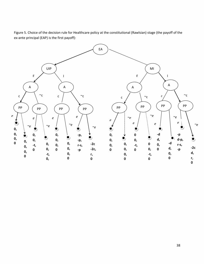
38

A

UIP

PP

A

c c ~c

MI

PP PP PP

A A

PP PP PP

I E E I

~c ~c ~c c

e e

e e

e e e

~e ~e ~e ~e

~e

~e

~e ~e

0,

0,

-t,

0,

0

0,

0,

-t,

0

0,

0,

0,

0

0,

0,

0,

0

0,

0,

0,

0

-p,

-p,

r-s,

-p

-2c

-2c,

r,

0

0,

0,

0,

0

0,

0,

0,

0

0

0,

-t,

0

0

0,

-t,

0

-d

d,

0,

0

-d

d,

0,

0

-p

d-p,

r-s,

-p -2c

d,

r,

0

PP

0,

0,

0,

0

e

c

EA

Figure 5. Choice of the decision rule for Healthcare policy at the constitutional (Rawlsian) stage (the payoff of the

ex-ante principal (EAP) is the first payoff):

Challenges to the standard Euclidean spatialmodel∗

Jon X. Eguia†

New York University

August 26, 2012

∗This working paper is meant to be published as a chapter in the volume “Advances inPolitical Economy”, edited by G. Caballero, D. Kselman and N. Schofield. I thank ScottTyson for suggestions. Comments to ammend errors or to provide updates to the workingpaper are welcome even after the publication of the volume.

†eguia@nyu.edu 19 West 4th, 2nd floor. New York, NY 10012, US.

1

1 Introduction

Spatial models are useful to represent political competition over policy issues.

If the feasible policies over a given policy issue are endowed with a natural

left/right or low/high order, we can represent the set of feasible policies by

a subset of the real line. Many policy issues are indeed easily ordered: tax

rates can vary from 0% to 100%; any budgeted policy item can receive a

lower or higher budget; criminal law can specify lighter or harsher sentences;

etc. It is standard to assume that agents have a unique ideal policy and

that given two policies below the agent’s ideal policy, or given two policies

above the agent’s ideal policy, the agent prefers the policy closer to the

agent’s ideal. Preferences satisfying this assumption are single-peaked. If

agents’ preferences are single peaked over the real line, simple majority rule

is transitive (Black [6]); furthermore, the median ideal policy among all the

agents’ ideal policies defeats any other policy if the number of agents is

odd and it cannot be defeated by any other policy when preferences are

aggregated by majority rule (Black [7]). Since the median policy cannot be

defeated by any other, electoral competition between two candidates leads to

policy convergence: both candidates choose the median policy (Downs [15],

building on Hotelling’s [24]), even if the candidates have diverging policy

2

preferences (Wittman [61], Calvert [9]).

Political competition usually involves multiple policy issues. Candidates

propose policy bundles with one policy per issue. Multidimensional spa-

tial models represent preferences over policy bundles: each dimension corre-

sponds to a given issue. Starting with Davis, DeGroot and Hinich [13], the

standard approach is to assume that agents have a most preferred alterna-

tive in the policy space, and utilities that are decreasing in the Euclidean

distance to this point, typically with a linear (Kramer [28], Wittman [60];

Patty, Snyder and Ting [43]; Degan and Merlo [14]; or Eguia [21]), quadratic

(Feddersen [22]; Clinton, Jackman and Rivers [11]; Schofield and Sened [53];

or Schofield [51] and [50]) or exponential (Poole and Rosenthal [45]) loss

function.1 Other theories allow for more general utility functions, but they

preserve the circular Euclidean shape of indifference curves (McKelvey [35]),

or they relax the assumption of circular indifference curves but maintain the

restrictions that utility functions be differentiable (Plott [44]; Schofield [49];

Duggan [16]; or Duggan and Kalandrakis [17]), quasiconcave (Banks and

Duggan [4]), or differentiable and quasiconcave (Kramer [27]).

1D’Agostino and Dardanoni ([12]) provide an axiomatization of the Euclidean distance;Azrieli ([3]) provides an axiomatization of Euclidean utilities with a quasilinear additivevalence term.

3

I present a series of theoretical and empirical results that challenge the as-

sumption that preferences over multiple issues can be adequately represented

by utility functions that are linear, quadratic or exponential Euclidean in a

multidimensional space. More generally, I present results that call into ques-

tion whether preferences can be represented by differentiable or quasiconcave

utility functions, let alone with Euclidean or weighted Euclidean utility func-

tions.

I divide these theoretical and empirical challenges to standard assump-

tions in three classes:

I. Concerns about the concavity of the loss function, accepting the Euclid-

ean shape of the indifference curves.

II. Concerns about the shape of indifference curves: convexity, and dif-

ferent weights for different dimensions.

III. Concerns about the shape of indifference curves: separability across

issues.

4

2 Concerns about the Loss Function

Circular indifference curves are a common assumption on preferences in mul-

tidimensional spatial models. Circular indifference curves are such that two

policy points which are at identical distances from an agent’s ideal point are

valued identically, i.e. the ‘direction’ of the perturbation from the agent’s

ideal point is inconsequential for his or her utility. This is a standard as-

sumption on indifference curves. However, no similar consensus exists on a

standard or default assumption on the loss function associated with these in-

difference curves. Linear or quadratic loss functions are the most commonly

used (McCarty and Meirowitz [34] section 2.5). As noted in the Introduction,

exponential functions are also used (Poole and Rosenthal [45]).2 The choice

of the functional form of the utility function in the various theories in the

literature appears motivated by convenience or simplicity.

The choice of loss functions is consequential: important results rely cru-

cially on the concavity of the loss function. For instance, in a probabilistic

voting model of electoral competition with two candidates, Kamada and

Kojima [26] show that in equilibrium candidates converge to the median if

2In support of their assumption of exponential utility functions, Poole and Rosenthal[46] argue that (standard) concave utility functions do not fit the data well.

5

voters’ utility functions are concave, but candidates diverge if voters’ utility

functions are sufficiently convex.

Osborne [42] warns that “the assumption of concavity is often adopted,

first because it is associated with ‘risk aversion’ and second because it makes

easier to show that an equilibrium exists. However, [...] it is not clear that

evidence that people are risk averse in economic decision-making has any

relevance here. I conclude that in the absence of any convincing empirical

evidence, it is not clear which of the assumptions is more appropriate.”

Seeking to test voters’ risk attitude, Berinski and Lewis [5] assume that

utility functions take the form ui(x, xk) = −d(x, x∗i )α, where d(x, x∗i ) is a

weighted Euclidean distance and α is a parameter to be estimated. They

find that the estimate that provides a best fit for voter choices in US pres-

idential elections is α ≈ 1, suggesting that it is appropriate to assume that

voters’ utilities are linear weighted Euclidean. They interpret this finding as

evidence that voters are risk neutral, but Eguia [19] casts axiomatic doubt

on this interpretation: linear Euclidean utilities do not satisfy additive sep-

arability, so the preferences over lotteries on a given issue and hence the

risk attitude of a voter with a linear Euclidean utility function depend on

outcomes on other issues. In other words, voters with multi-dimensional

6

linear Euclidean utilities are not risk neutral. With utilities that decrease

in weighted Euclidean distances, additive separability (i.e. independence of

preferences over lotteries on one issue with outcomes on other issues) requires

that the loss function be quadratic (Eguia [20]). The only way to reconcile

additive separability (which under Euclidean indifference curves requires a

quadratic loss function) with Berinski and Lewis’s [5] finding (with Euclidean

indifference curves a linear loss function provides the best fit) is to discard the

assumption of Euclidean indifference curves, and to check if under different

shapes of the indifference curves, we obtain a best fit with a parameter for

the loss function that is consistent with additive separability. This leads us

to the second class of concerns: concerns about the shape of the indifference

curves.

3 Concerns about Convexity of Preferences

A first concern about the assumption of utility functions that depend on the

Euclidean distance is that some issues may be more important than others,

and hence utilities ought to be weighted, generating elliptical (rather than

circular) indifference curves in the case with two dimensions. If all voters

7

assign the same weights to these dimensions, the problem is trivially solved,

and Euclidean circles reinstated, by rescaling the units of measure of each

dimension according to its weight. If different groups of voters assign different

relative weights to the various dimensions, then it is not possible to rescale

the dimensions so as to use unweighted Euclidean utilities, and we must

instead use weighted Euclidean utilities with different weights for different

voters (Miller and Schofield [38]).

A deeper concern is that preferences may not be representable by weighted

Euclidean utility functions: indifference curves may have shapes that are not

elliptical. Weighted Euclidean utilities represent a particular class of con-

vex preferences. Preferences are (strictly) convex if the upper contour set

defined by each indifference curve is (strictly) convex; that is, if the set of

policies preferable to policy x is convex, for any x. Representable (strictly)

convex preferences are representable by (strictly) quasiconcave utility func-

tions. If preferences are not strictly convex, they cannot be represented by

Euclidean utility functions, neither unweighted nor weighted ones. The cur-

vature imposed by Euclidean utilities is simply not adequate to represent the

preferences.

An alternative assumption to Euclidean preferences is city-block prefer-

8

ences, which define square indifference curves (with squares tilted at a 45

degree angle relative to the axes of coordinates), and are representable by

utility functions that are decreasing in the l1 distance ||x−x∗||1 =KPk=1

|xk−x∗k|,

where xk is the policy on issue k ∈ {1, ..., K}. That is, agents with city block

preferences calculate the distance between two points by adding up the dis-

tance dimension by dimension, as if traveling on a grid (that is why the l1

or city block distance is sometimes called “Manhattan distance”), and they

prefer points closer to their ideal according to this notion of distance. If pref-

erences are city block, their utility representation is not strictly quasiconcave,

and it is not differentiable. Classic results on the instability of simple ma-

jority rule (Plott [44], McKelvey [35]) do not apply if agents have city block

preferences. In fact, the core of simple majority rule is not empty under more

general conditions if agents have city-block preferences (Rae and Taylor [47];

Wendell and Thorson [58]; McKelvey and Wendell [37]; and Humphreys and

Laver [25]).

Humphreys and Laver [25] invoke results from psychology and cognitive

sciences (Shepard [56]; Arabie [1]) to argue that agents measure distance to

objects with separable attributes by adding up the distance in each attribute,

which implies that if the object under consideration is a policy bundle on

9

separable issues, agents measure distance according to the city block function.

Grynavisky and Corrigan [23] find that a model that assumes voters have

city block preferences provides a better fit of vote choice in US presidential

elections than an alternative model that assumes voters have linear Euclidean

preferences. Westholm [59] finds that a model with city block preferences

outperforms a model with quadratic Euclidean preferences, when aiming to

predict vote choice in Norwegian elections. However, a binary comparison

between city block utilities based on the l1 metric ||x − x∗||1 =KPk=1

|xk −

x∗k| and the linear Euclidean utilities based on the l2 metric ||x − x∗||2 =µKPk=1

(xk − x∗k)2

¶ 12

is unnecessarily restrictive: l1 and l2 are special cases of

the Minkowski [41] family of metric functions, which parameterized by δ,

gives the distance between x and x∗ as:

||x− x∗||δ =Ã

KXk=1

(xk − x∗k)δ

!1δ

. (1)

Rather than comparing δ = 1 (linear city block) and δ = 2 (linear Euclidean),

it appears more fruitful to estimate parameter δ. Rivero [48] estimates δ for

several Spanish regional elections and finds that δ ∈ (0.92, 1.17); none of the

estimates is significantly different from δ = 1, and they are all significantly

10

different from δ = 2. These tests support the use of linear city block over

linear Euclidean utility functions.

Utility functions that are linearly decreasing in expression (1) are not

additively separable unless δ = 1. To satisfy additive separability, the utility

function must be linearly decreasing in the δ power of ||x− x∗||δ, so that

u(x, x∗) = −KXk=1

(xk − x∗k)δ, (2)

with linear city block utilities corresponding to δ = 1, and quadratic

Euclidean to δ = 2. Notice that any parameter δ > 1 results in strictly con-

vex preferences and strictly quasiconcave and differentiable utility functions,

while δ < 1 results on preferences that are not convex, and utility functions

that are neither strictly quasiconcave, nor differentiable. Ye, Li and Leiker

[62] estimate parameter δ using the utility function (2) and voting data from

the American National Election Studies corresponding to the 2000, 2004 and

2008 Presidential elections. However, their results are inconclusive, obtain-

ing estimates that vary greatly across elections and, most puzzlingly, across

candidates.

Further empirical work appears necessary to establish which utility func-

11

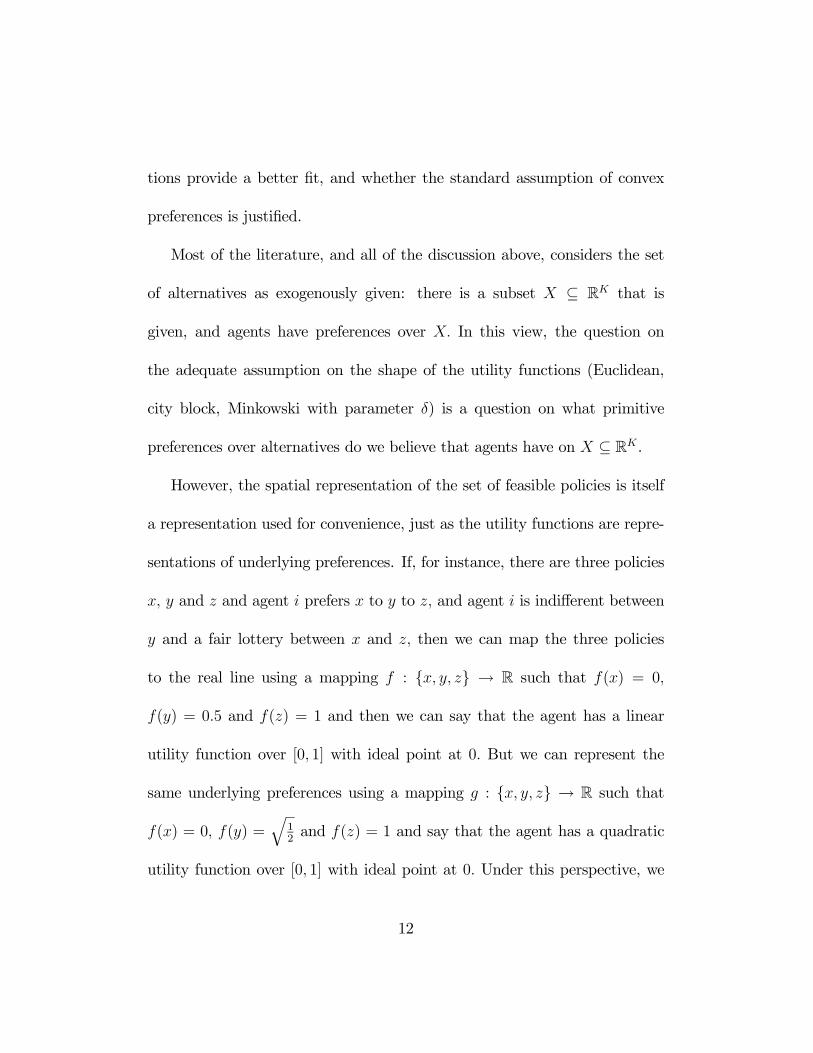
tions provide a better fit, and whether the standard assumption of convex

preferences is justified.

Most of the literature, and all of the discussion above, considers the set

of alternatives as exogenously given: there is a subset X ⊆ RK that is

given, and agents have preferences over X. In this view, the question on

the adequate assumption on the shape of the utility functions (Euclidean,

city block, Minkowski with parameter δ) is a question on what primitive

preferences over alternatives do we believe that agents have on X ⊆ RK .

However, the spatial representation of the set of feasible policies is itself

a representation used for convenience, just as the utility functions are repre-

sentations of underlying preferences. If, for instance, there are three policies

x, y and z and agent i prefers x to y to z, and agent i is indifferent between

y and a fair lottery between x and z, then we can map the three policies

to the real line using a mapping f : {x, y, z} → R such that f(x) = 0,

f(y) = 0.5 and f(z) = 1 and then we can say that the agent has a linear

utility function over [0, 1] with ideal point at 0. But we can represent the

same underlying preferences using a mapping g : {x, y, z} → R such that

f(x) = 0, f(y) =q

12and f(z) = 1 and say that the agent has a quadratic

utility function over [0, 1] with ideal point at 0. Under this perspective, we

12

see that the shape of the utility function is an object of choice for the the-

orist who wishes to study an individual: using a different mapping of the

set of alternatives into a vector space leads to indifference curves of different

shapes. The spatial representation of the set of alternatives and the utility

function we use in this space jointly determine the assumptions we make on

the underlying preferences of the agent.

Once we recognize that the spatial representation of the set of alterna-

tives is an endogenous choice made by the theorist who wishes to model

preferences, we can ask new questions: can all preferences over policies be

represented by Euclidean utility functions in some space? if not, what pref-

erences can be represented by Euclidean utility functions? If we accept a

spatial representation with great dimensionality, we obtain a positive result:

any preference profile with N agents can be represented by utility functions

that are Euclidean for all N agents if we let the mapping of the set of alter-

nativesX into RK containK ≥ N dimensions (Bogomolnaia and Laslier [8]).

If we care for the number of dimensions in our spatial representation, we do

not obtain such a positive result. Suppose the policy issues are exogenously

given, and we want to use no more than one dimension per issue in our spa-

tial representation. In this case, while we can represent any single-peaked,

13

separable preference relation of a single individual using quadratic Euclidean

utility functions over an appropriately chosen spatial representation of the

set of alternatives, we cannot represent the preferences of all N individu-

als with quadratic Euclidean utility functions in any spatial representation

unless the underlying preference profile satisfies very restrictive conditions

(Eguia [18]).3

For any preference profile, we can always map the set of alternatives into

RK so as to represent the preferences of a given agent by quasiconcave utility

functions over the chosen map. However, depending on the preference profile,

any mapping that achieves this may be such that the utility representations

of the preferences of other agents violate quasiconcavity and/or differentia-

bility. Whether preference profiles in any given application are such that the

preferences of all agents can be represented in some map with quasiconcave

utility functions is an open empirical question.

3Calvo, Hellwig and Chang [10] analyze an additional complication: agents may notagree on which alternative is to the right or left of another on a given issue. If so, wecannot use a unique spatial representation; rather, we must have subjetive maps of the setof the set of alternatives, one for each agent.

14

4 Concerns about Separability of Preferences

Expressions (1) or (2) above, or variations with weights for each dimension,

allow us to relax the assumption that indifference curves have circular or

elliptical curvature. We are free to assume any degree of curvature, including

preferences that are not convex by choosing δ < 1. These generalizations of

the standard model from δ = 2 to any δ > 0 preserve the assumption that

preferences are separable across issues: ordinal preferences over alternatives

on a given issue do not depend on the realized outcome on other issues.

Milyo [40] and [39] notes that preferences over multiple dimensions of

public spending cannot possibly be separable. Suppose a fixed unit of na-

tional income is to be allocated between public spending on policy one, public

spending on policy two, and private consumption. Decreasing marginal util-

ity over consumption of public goods means that as public spending on policy

one increases, the opportunity cost of spending on issue two also increases, so

the ideal amount of expenditures on issue two must decrease with the amount

spent on issue one. Preferences over public spending on issues one and two

cannot be separable. This problem is easily solved by redefining the policy

dimensions over which we assume that agents have separable preferences: let

the first dimension be total public spending, and let the second dimension be

15

the fraction of public spending devoted to issue one. Preferences may well

be separable under this representation of the set of issues, and in any case

they escape Milyo’s [40] and [39] critique.

A more insidious difficulty arises if preferences are truly non-separable,

not due to budgetary concerns, but because agents’ ideal values on a given

issue actually depend on the outcomes on other issues. For instance, it

is possible that agents have non-separable preferences about immigration

policy and the social safety net, preferring a more generous safety net if

immigration policy is restrictive so redistributive policies benefit only natives,

than if immigration policy is lax so redistributive policies would in part favor

immigrants. Lacy [31] and [32] and [33] uncovers evidence of such non-

separability across various pairs of issues.

If agents have non-separable preferences, but the correlation between is-

sues is the same for all agents, then the problem is addressed by considering

new, endogenous policy dimensions over which agents have separable prefer-

ences. Suppose that there are two complementary issues, such that for any

agent i,

u(x1, x2) = −(x1 − xi1)2 − (x2 − xi2)

2 + (x1 − xi1)(x2 − xi2).

16

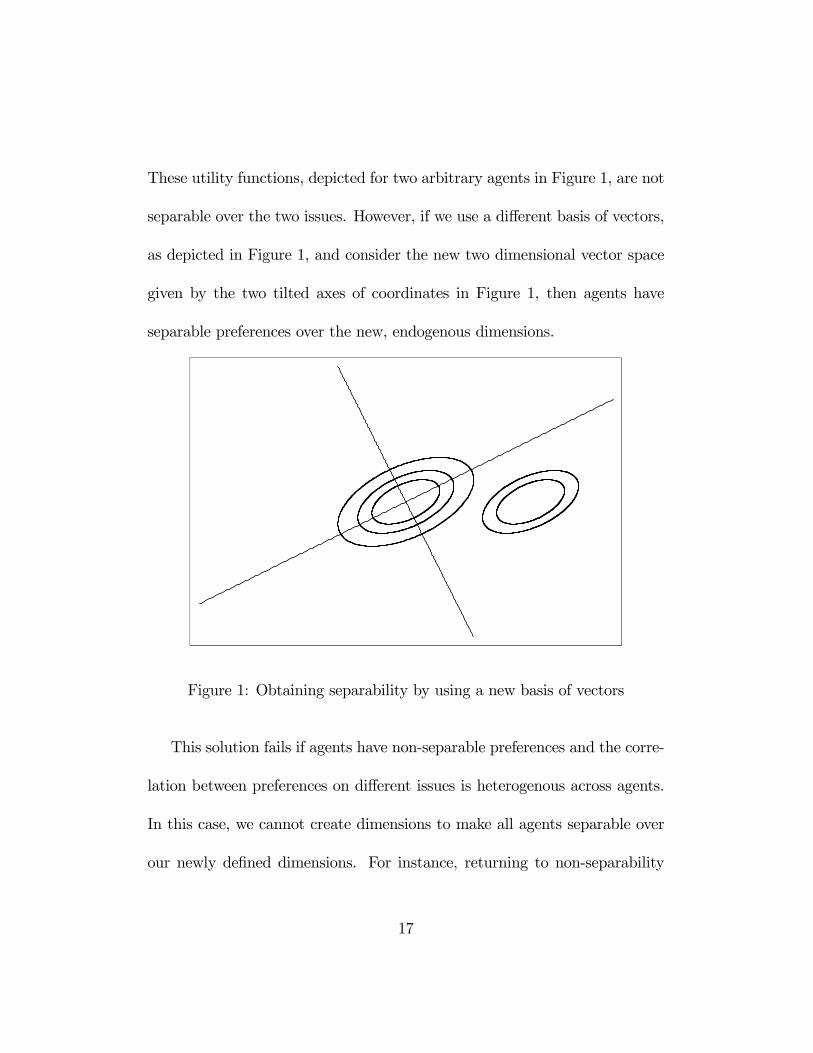
These utility functions, depicted for two arbitrary agents in Figure 1, are not

separable over the two issues. However, if we use a different basis of vectors,

as depicted in Figure 1, and consider the new two dimensional vector space

given by the two tilted axes of coordinates in Figure 1, then agents have

separable preferences over the new, endogenous dimensions.

Figure 1: Obtaining separability by using a new basis of vectors

This solution fails if agents have non-separable preferences and the corre-

lation between preferences on different issues is heterogenous across agents.

In this case, we cannot create dimensions to make all agents separable over

our newly defined dimensions. For instance, returning to non-separability

17

between immigration and social safety net, if some agents prefer a larger

safety net to help needy immigrants when immigration policy is lax, while

other agents prefer a smaller safety net to not spend money on immigrants

when immigration policy is lax, then we can redraw the axes to make the

preferences of one group of agents separable, but in doing so, the preferences

of the other group of agents remain non-separable. In very non-technical

terms, agents have non-separable preferences if their indifference curves are

tilted; if all agents have curves equally tilted, we can tilt the whole map to

return to a standard model over newly defined dimensions.

If, on the contrary, different agents have preferences tilted in different

directions, we cannot correct this problem by tilting the whole map. We

need instead to introduce parameters to accommodate the correlation across

issues. This is a considerable setback, similar to the problem of agents who

assign different relative weights to the various dimensions -but more dam-

aging, because we need more parameters to fix it. In order to accurately

represent the preferences of agents who disagree on the weights they assign

to the different dimensions we need to add one parameter per dimension per

agent or group of agents who disagree on these weights, for a maximum of

(K − 1)(N − 1) new parameters if there are N agents and K dimensions. In

18

order to represent the preferences of agents who disagree on the correlation

in preferences between issues, we must add one correlation parameter per

possible pair of issues and per agent or group of agents who disagree, for a

maximum of K(K−1)2

N new parameters.

While violations of separability do not affect classic results on the insta-

bility of simple majority rule as long as preferences are smooth (Plott [44],

McKelvey [36]), they affect how we can interpret and use common spatial

models. Consider the structured-induced equilibrium theory (Shepsle and

Weingast [57]), which proposes that the instability is solved by choosing pol-

icy dimension by dimension. In the standard structured-induced equilibrium

theory, the order in which the legislature considers the various policy dimen-

sions is irrelevant, because preferences are separable. With non-separable

preferences, the order in which each policy dimension is considered affects

the chosen policy outcome. For a second example, consider the ideal point es-

timation literature (Poole and Rosenthal [45]; Clinton, Jackman and Rivers

[11]): if preferences are not separable, estimating the ideal point of each

legislator is not enough to predict vote choice.

19

5 Discussion

Theoretical and empirical work questions not only the standard assumption

of Euclidean utility functions in multidimensional spatial models, but the

more general assumptions of separable, convex and/or smooth preferences.

Standard spatial models suffer from limitations that I have not consid-

ered here. For instance, an increasing body of literature argues that we must

add a candidate valence term to capture the actual preferences of voters

about candidates. Valence is any quality that all voters agree is good, and

makes the candidate who possesses more of it more attractive to all voters.

Current research on valence seeks to endogenize it and to analyze its rela-

tion to the candidate’s spatial location (Ashworth and Bueno de Mesquita

[2]; Zakharov [63]; Serra [54] and [55]; Krasa and Polborn [29] and [30]; or

Schofield, Classen, Gallego and Ozdemir [52]). In this chapter I analyze con-

cerns about a basic pillar of the spatial model: the assumption that agents

have preferences over a vector space that represents the set of feasible policies,

preferences that can be represented by analytically convenient utility func-

tions. Valence, dynamics, uncertainty, bounded rationality, other-regarding

preferences or other improvements can be added to the basic spatial model

to generate richer theories, but any theory with a spatial component must

20

address the challenges posed in this chapter about the appropriate formal-

ization of spatial preferences in the theory.

Further empirical work is necessary to establish whether agents have con-

vex preferences over policy bundles with multiple policy issues. Assuming the

functional form (1) or, if we want to satisfy additive separability, functional

form (2) for the utility functions, empirical work must estimate parameter δ.

If the estimated parameter δ is less than 1, the consequences for theoretical

work are dramatic: Preferences are not convex, and hence utility functions

are neither quasiconcave, nor differentiable. Standard results in the litera-

ture that rely on these assumptions, most notably the instability of majority

rule (Plott [44]; McKelvey [35]; Schofield [49]), would not apply. Whereas,

results that rely on city block preferences (Humphreys and Laver [25]) or on

non-differentiable utility functions (Kamada and Kojima [26]) would become

more relevant, and further theoretical work would be needed to establish

what results in the literature obtained under assumptions of quasiconcavity

or differentiability of preferences are robust and apply in environments with

agents whose preferences are not representable by quasiconcave or differen-

tiable utility functions.

If the estimated parameter δ is consistently greater than 1,even if it is

21

not near 2, much of the theoretical literature will be validated. The main

impact of obtaining a better estimate of δ in utility functions of the form (2)

that is δ 6= 2 but δ > 1 will be to improve the fit of further empirical work on

ideal point estimation models (Clinton, Jackman and Rivers [11]; Poole and

Rosenthal [45]), or vote choice models, by assuming that agents have utility

functions with the curvature corresponding to the best estimate of δ within

the parameterized family of utility functions (2), instead of assuming that

agents have utility functions with parameter δ = 2 even though parameter

δ = 2 provides a poorer fit for the model.

With regard to separability, violations of the assumption typically do not

affect equilibrium existence or convergence results on models of electoral com-

petition or policy choice. However, application of spatial models to specific

real world polities or electorates should take into account existence evidence

on non-separability across various pairs of issues (Lacy [31] and [32] and [33]),

so that if the models explicitly include such issues, utility functions are not as-

sumed to be separable over them. Many spatial models do not include many

issues; rather, they collapse the list of all issues onto two dimensions, one that

groups economic issues (from left/pro-state to right/pro-market) and another

that includes all cultural issues (from left/progressive to right/conservative).

22

It is more difficult to determine whether preferences are separable or not over

such dimensions, which are not precisely defined. Nevertheless, if future em-

pirical work reveals evidence of a systematic correlation between preferences

across economic and cultural issues, models should either seek to define new

dimensions (new ways of bundling or weighing the issues) in such a way that

preferences are separable over the new dimensions, or else, if this cannot be

achieved, then it may be necessary to allow for non-separable preferences,

estimating not only an ideal point, but also a degree of correlation between

dimensions for each agent or group of agents.

Euclidean preferences have been an extremely useful tool in the develop-

ment of multidimensional spatial models that can explain electoral compe-

tition, government formation and legislative policy-making. Generalizations

that show that several theoretical results are robust if preferences are not

Euclidean but are convex and smooth allowed us to conjecture that Euclid-

ean preferences are only a simplifying shortcut with limited effect on our

ability to understand the political processes we model. Nevertheless, we lack

convincing empirical evidence that preferences are convex and smooth. If

preferences are not convex and smooth, nor separable, and our theoretical

models assume that they are, we are impaired in our ability to understand

23

and predict the political processes we study.

Future empirical work shall establish whether preferences are convex and

smooth, and whether we can find systematic evidence of differentiated non-

separability over pairs of issues, or systematic differences in the weights as-

signed to different dimensions, across different groups of voters or legislators.

Future (better) theories must make assumptions that are consistent with

these future empirical findings.

References

[1] Phipps Arabie. Was Euclid and Unnecessarily Sophisticated Psycholo-

gist? Psychometrika, 56(4):567—587, 1991.

[2] Scott Ashworth and Ethan Bueno de Mesquita. Elections with Platform

and Valence Competition. Games and Economic Behavior, 67(1):191—

216, 2009.

[3] Yaron Azrieli. Axioms for Euclidean Preferences with a Valence Dimen-

sion. Journal of Mathematical Economics, 47(4-5):545—553, 2011.

24

[4] Jeffrey S. Banks and John Duggan. A Dynamic Model of Democratic

Elections in Multidimensional Policy Spaces. Quarterly Journal of Po-

litical Science, 3:269—299, 2008.

[5] Adam J. Berinsky and Jeffrey B. Lewis. An Estimate of Risk Aversion in

the U.S. Electorate. Quarterly Journal of Political Science, 2:139—154,

2007.

[6] Duncan Black. On the Rationale of Group Decision-Making. Journal of

Political Economy, 56(1):23—34, 1948.

[7] Duncan Black. The Theory of Committees and Elections. London, Cam-

bridge University Press, 1958.

[8] Anna Bogomolnaia and Jean-François Laslier. Euclidean Preferences.

Journal of Mathematical Economics, 43:87—98, 2007.

[9] Randall Calvert. Robustness of the Multidimensional Voting Model:

Candidate Motivations, Uncertainty and Convergence. American Jour-

nal of Political Science, 29:69—95, 1985.

[10] Ernesto Calvo, Timothy Hellwig, and Keyoung Chang. The eye of the

beholder: Ideological lensing, information effects, and the vote. Fun-

25

dacion Juan March conference on Contemporary Applications of the

Spatial Model, 2012.

[11] Joshua D. Clinton, Simon D. Jackman, and Douglas Rivers. The Statis-

tical Analysis of Roll Call Data: A Unified Approach. American Political

Science Review, 98:355—370, 2004.

[12] Marcello D’Agostino and Valentino Dardanoni. What’s so Special about

Euclidean Distance? Social Choice and Welfare, 33(2):211—233, 2009.

[13] Otto A. Davis, Morris H. DeGroot, and Melvin J. Hinich. Social Prefer-

ence Orderings and Majority Rule. Econometrica, 40(1):147—157, 1972.

[14] Arianna Degan and Antonio Merlo. Do Voters Vote Ideologically? Jour-

nal of Economic Theory, 144(5):1868—1894, 2009.

[15] Anthony Downs. An Economic Theory of Political Action in a Democ-

racy. The Journal of Political Economy, 65(2):135—150, 1957.

[16] John Duggan. Equilibrium Existence for Zero-sum Games and Spatial

Models of Elections. Games and Economic Behavior, 60:52—74, 2007.

[17] John Duggan and Tasos Kalandrakis. Dynamic Legislative Policy Bar-

gaining. Journal of Economic Theory, pages —, 2012.

26

[18] Jon X. Eguia. On the Spatial Representation of Preference Profiles.

Economic Theory, pages —.

[19] Jon X. Eguia. Utility Representations of Risk Neutral Preferences in

Multiple Dimensions. Quarterly Journal of Political Science, 4(4):379—

385, 2009.

[20] Jon X. Eguia. Foundations of Spatial Preferences. Journal of Mathe-

matical Economics, 47(2):200—205, 2011.

[21] Jon X. Eguia. A Spatial Theory of Party Formation. Economic Theory,

49(3):549—570, 2012.

[22] Timothy J. Feddersen. A Voting Model Implying Duverger’s Law and

Positive Turnout. American Journal of Political Science, 36(4):938—962,

1992.

[23] Jeffrey D. Grynaviski and Bryce E. Corrigan. Specification Issues in

Proximity Models of Candidate Evaluation (with Issue Importance). Po-

litical Analysis, 14:393—420, 2006.

[24] Harold Hotelling. Stability in Competition. Economic Journal,

39(153):41—57, 1929.

27

[25] Macartan Humphreys and Michael Laver. Spatial Models, Cognitive

Metrics and Majority Rule Equilibria. British Journal of Political Sci-

ence, 40(1):11—30, 2009.

[26] Yuichiro Kamada and Fuhito Kojima. Voter Preferences, Polarization

and Electoral Policies. working paper, Jan 2010.

[27] Gerald H. Kramer. On a Class of Economic Conditions for Majority

Rule. Econometrica, 41(2):285—297, 1973.

[28] Gerald H. Kramer. A Dynamical Model of Political Equilibrium. Journal

of Economic Theory, 16(2):310—334, 1977.

[29] Stefan Krasa and Mattias Polborn. Competition Between Specialized

Candidates. American Political Science Review, 104(4):745—765, 2010.

[30] Stefan Krasa and Mattias Polborn. Political Competition Between Dif-

ferentiated Candidates. Games and Economic Behavior, pages —, Forth-

coming.

[31] Dean Lacy. A Theory of Nonseparable Preferences in Survey Responses.

American Journal of Political Science, 45(2):239—258, 2001.

28

[32] Dean Lacy. Nonseparable Preferences, Measurement Error, and Unsta-

ble Survey Responses. Political Analysis, 9(2):1—21, 2001.

[33] Dean Lacy. Nonseparable preferences, issue voting, and issue packag-

ing in elections. Fundacion Juan March conference on Contemporary

Applications of the Spatial Model, 2012.

[34] Nolan McCarty and Adam Meirowitz. Political Game Theory. Cam-

bridge University Press, 2007.

[35] Richard D McKelvey. Intransitivities in Multidimensional Voting Mod-

els and Some Implications for Agenda Control. Journal of Economic

Theory, 12:472—482, 1976.

[36] Richard D. McKelvey. General Conditions for Global Intransitivities in

Formal Voting Models. Econometrica, 47(5):1085—1112, 1979.

[37] Richard D. McKelvey and Richard E. Wendell. Voting Equilibria in

Multidimensional Choice Spaces. Mathematics of Operations Research,

1(2):144—158, 1976.

29

[38] Gary Miller and Norman Schofield. Activists and Partisan Realignment

in the United States. American Political Science Review, 97(2):245—260,

2003.

[39] Jeffrey Milyo. A Problem with Euclidean Preferences in Spatial Models

of Politics. Economic Letters, 66(2):179—182, 2000.

[40] Jeffrey Milyo. Logical Deficiencies in Spatial Models: A Constructive

Critique. Public Choice, 105(3-4):273—289, 2000.

[41] Hermann Minkowski. Geometrie der Zahlen. Leipzig, Teubner Verlag,

1886.

[42] Martin Osborne. Spatial Models of Political Competition under Plu-

rality Rule: A Survey of Some Explanations of the Number of Candi-

dates and the Positions They Take. Canadian Journal of Economics,

28(2):261—301, 1995.

[43] John W. Patty, James M. Snyder, and Michael M. Ting. Two’s Com-

pany, Three’s an Equilibrium: Strategic Voting and Multicandidate

Elections. Quarterly Journal of Political Science, 4(3):251—278, 2009.

30

[44] Charles R. Plott. A Notion of Equilibrium and its Possibility under

Majority Rule. American Economic Review, 57(4):331—347, 1967.

[45] Keith Poole and Howard Rosenthal. A Spatial Model for Roll Call

Analysis. American Journal of Political Science, 29:331—347, 1985.

[46] Keith T. Poole and Howard Rosenthal. Congress: A Political-Economic

History of Roll Call Voting. Oxford University Press, 1997.

[47] Douglas W. Rae and Michael Taylor. Decision Rules and Policy Out-

comes. British Journal of Political Science, 1:71—90, 1971.

[48] Gonzalo Rivero. Integrality and separability in multidimensional voting

models: Ideology and nationalism in spanish regional elections. Cen-

ter for Advanced Study in the Social Sciences, Fundacion Juan March,

2011/265, December 2011.

[49] Norman Schofield. Instability of Simple Dynamic Games. Review of

Economic Studies, 40(3):575—594, 1978.

[50] Norman Schofield. Political Equilibria with Electoral Uncertainty. Social

Choice and Welfare, 28:461—490, 2007.

31

[51] Norman Schofield. The Mean Voter Theorem: Necessary and Sufficient

Conditions for Convergent Equilibrium. Review of Economic Studies,

74:965—980, 2007.

[52] Norman Schofield, Christopher Claassen, Maria Gallego, and Ugur

Ozdemir. Political Economy of Institutions, Democracy and Voting,

chapter Empirical and Formal Models of the United States Presidential

Elections in 2000 and 2004. Ed. N. Schofield and G. Caballero. Springer,

2011.

[53] Norman Schofield and Itai Sened. Multiparty Democracy. Cambridge

University Press, 2006.

[54] Gilles Serra. Polarization of What? A Model of Elections with Endoge-

nous Valence. The Journal of Politics, 72(2):426—437, 2010.

[55] Gilles Serra. Does charisma discourage experience? an election with two

types of valence. ICOPEAI II Conference paper, 2012.

[56] Roger N. Shepard. Toward a Universal Law of Generalization for Psy-

chological Science. Science, 237:1317—1323, 1987.

32

[57] Kenneth A. Shepsle and Barry R. Weingast. Structure-iInduced Equi-

librium and Legislative Choice. Public Choice, 37(3):503—519, 1981.

[58] Richard E. Wendell and Stuart J. Thorson. Some Generalizations of

Social Decisions under Majority Rule. Econometrica, 42:893—912, 1974.

[59] Anders Westholm. Distance versus Direction: The Illusory Defeat of

the Proximity Theory of Electoral Choice. American Political Science

Review, 91(4):865—883, 1997.

[60] Donald Wittman. Candidates with Policy Preferences: A Dynamic

Model. Journal of Economic Theory, 14(1):180—189, 1977.

[61] Donald Wittman. Candidate Motivation: A Synthesis of Alternatives.

American Political Science Review, 77(1):142—157, 1983.

[62] Min Ye, Quan Li, and Kile W. Leiker. Evaluating Voter-Candidate Prox-

imity in a Non-Euclidean Space. Journal of Elections, Public Opinion

and Parties, 4:497—521, 2011.

[63] Alexei Zakharov. A Model of Candidate Location with Endogenous

Valence. Public Choice, 138:347—366, 2009.

33

40

A Non-Existence Theorem for Clientelism in Spatial Models

Daniel Kselman, Center for Advanced Studies in the Social Sciences

Juan March Institute dksleman@march.es

I. Introduction

In spatial models of political competition, political parties typically announce

positions on one or more issue dimensions; voters then choose from among these parties

according to their preferences over the same issue dimensions. Put otherwise, spatial

models typically analyze programmatic elections in which the link between voter choice

2

and elite behavior is consummated indirectly, via collectively applicable policy issues.1

In contrast, a growing body of research in comparative politics and comparative political-

economy investigates clientelistic linkages between citizens and elected officials. Such

linkages are grounded not in national-level public policy debates, but rather in a direct

and contingent exchange of votes (or other forms of political participation…) for tangible

material or professional rewards. These inducements take many forms: jobs in the public

sector, access to the electric grid, washing machines, alcohol, fuel, etc. In such contexts,

in addition to evaluating political parties’ policy stances on one or more programmatic

issues, voters choose based on parties’ ability to provide targeted inducements.

A series of recent papers, reviewed in Section II below, have analyzed clientelism

in a game theoretic setting. While all make valuable contributions to the literature on

contingent electoral exchange, none explicitly introduces clientelistic concerns into the

traditional spatial model, which has for decades been the work-horse in formal political

theory. This paper develops a spatial model in which political parties strategically

choose: (1) their programmatic policy position, (2) the effort they devote to clientelism as

opposed to the promotion of their programmatic position, and (3) the set of voters who

are targeted to receive clientelistic benefits. Section III presents the model’s actors, their

utility functions, and the actions which comprise their choice sets. Section IV then

demonstrates that, absent stronger restrictions on candidate behavior, there will never

exist Nash Equilibria with positive clientelistic effort: given some clientelistic proposal

1 A similar accountability mechanism underpins the ‘Responsible Party Government’ model, which dates at least to Lipsett and Rokkan (1967), and sees ties between political parties and voters as grounded in campaign and governance strategies on issues of national-level public policy.

3

by their opponent, candidates can always propose a slightly ‘narrower’ set of recipients

and win an electoral plurality.

This is not to say that the game in its most general form is always characterized

by instability. On the contrary, if voter elasticity to clientelistic resources is sufficiently

low, then the game’s Nash Equilibrium will be for all candidates to choose the median

voter’s ideal point, and to devote 100% of their campaign effort to promoting this

platform. Thus, the game in its most general form yields either traditional median voter

convergence or theoretical instability. Section V relates this general result to past

literature on instability in coalition formation processes. It also discusses a set of

necessary conditions for the emergence of Nash Equilibria with positive levels of

clientelism. One condition is that parties have differential abilities to target distinct

subsets of voters. A second condition is that political parties face a binding turnout

constraint. When turnout is not a given and parties have differential ability to target

distinct subsets of voters, the need to balance one’s interest in courting the electoral

median with that in maintaining the support of one’s ideological base leads, at times, to

the adoption of positive equilibrium levels of clientelism.

II. Theories of Clientelism

So as to highlight this paper’s specific contributions, here I briefly outline recent

theoretical research on the causes of clientelism. In the Introduction to their edited

volume, Kitschelt and Stevenson (2007) present an argument to explain the mix of

clientelistic and programmatic appeals in politicians’ vote production functions. Driving

this mix is the interaction between economic development and electoral competitiveness.2

2 Competitiveness is a notably tricky concept to precisely define and operationalize. Different authors have assigned the concept different empirical referents. Kitschelt and Stevenson (2007) define competitive

4

At low levels of economic development politics is heavily clientelistic, and increasingly

so as competitiveness increases. At high levels of economic development, politics is

heavily programmatic and increasingly so as competitiveness increases. Finally, it is at

intermediate levels of development that politicians invest more equitably in both forms of

linkage. To complement these basic comparative statics, the authors also highlight the

role of a publicly controlled political-economy and formal political institutions in

conditioning the mix of linkage strategies.

In the same volume Magaloni et al. (2007) develop a decision-theoretic model to

consider an incumbent politician’s decision to generate public as opposed to clientelistic

goods. Public goods offer the ability to target large number of voters, but are risky insofar

as voters’ response to public good proposals is uncertain. On the other hand, clientelistic

goods allow politicians to gain smaller blocs of voter support with certainty. The optimal

allocation of clientelistic effort thus increases in: a.) voters’ relative preferences for

small-scale targeted policy goods (for which economic development should be a

reasonable proxy); b.) the relative uncertainty of vote returns to public good provision;

and c.) politicians’ risk aversion.

These papers emphasize the role of economic development, electoral

competitiveness, and incumbents’ risk profile in conditioning politicians’ optimal mix of

clientelistic and programmatic electoral appeals. They do not, however, investigate the

relationship between clientelistic appeals and the relative extremism or moderation of

political parties’ programmatic stances; nor the processes by which candidates choose

which segments of the electorate to target with clientelistic goods. Finally, they do not

elections as those in which “…elections are close between rival blocs of parties…and there is market of uncommitted voters sufficiently large to tip the balance in favor of one or another bloc.” (pg. 28)

5

embed the linkage decision in a strategic context such that one parties’ electoral strategies

are an explicit function of their competitors’ decisions.

Stokes (2005) analyzes an infinitely-repeated prisoner’s dilemma played between

an incumbent politician and a potential supporter, where the incumbent decides between

providing a benefit ‘B’ and the potential supporter decides to vote for the incumbent or a

challenger candidate. In equilibrium, clientelistic relationships of vote targeting are more

likely to arise when: a.) the benefit B is large; b.) voters are ‘moderate’ supporters of the

incumbent, i.e. not heavily biased for or against the incumbent’s programmatic policy

stances; and c.) when the ideological distance between the incumbent party and her

competitor shrinks. Nichter (2008) analyzes a similar model with one major distinction:

the game is played between an incumbent politician and a potential voter whose basic

decision is not who to choose but whether or not to turnout. Rather than targeting

‘moderate’ supporters, politicians who use clientelism to increase turnout are more likely

to do so among ‘strong’ ideological supporters. As well, the likelihood of clientelism

effectively inducing turning out is no longer a function of the ideological distance

separating incumbent and challenger candidates.

This first set of game theoretic papers has made valuable contributions to research

on the nature of parties’ clientelistic constituencies, i.e. the particular voters or subsets of

voters to which parties’ devote their clientelistic efforts. However, it does not address the

question asked by Kitschelt and Stevenson (2007) and Magaloni et al. (2007), namely

“What is politicians’ optimal mix between clientelistic and programmatic campaign

strategies?” Furthermore, it does not address the relationship between a party’s linkage

strategies and the relative extremism of its programmatic stances. Indeed, models by

6

Stokes (2005) and Nichter (2008) stipulate political parties’ spatial positions as

exogenously fixed, and from these fixed positions identify the subsets of ‘moderate’ and

‘strong’ party supporters. In model derived below the choice of programmatic stances is

explicit, such that the identity of ‘moderate’ and ‘strong’ party ideological supporters

arises as an endogenous outcome of strategic competition.

Keefer and Vlaicu (2008) adapt a particular political-economic model (Persson

and Tabellini 2000) to the comparative study of fiscal policy under alternative credibility

environments. Politicians in their model choose: a.) a level of public good provision; b) a

level of targeted good provision; c.) the set of districts to which targeted goods will be

allocated; and d.) rent extraction levels. Not unlike Stokes (2008), the authors find that

clientelism will be targeted to electoral districts with low levels of ideological bias, i.e.

those districts in which voters are more effectively swayed by targeted policy appeals.

They also find that a ‘broader’ segment of the electorate will be targeted as parties devote

more overall effort to clientelistic appeals, i.e. targeting becomes more ‘inclusive’ as

clientelistic effort increases. Finally, they argue that such appeals will be more prevalent

in systems where national-level politicians lack credibility on matters of economic

governance; and that they will tend to open the door to rent-seeking by public officials.3

Keefer and Vlaicu (2008) come closest to addressing the set of questions tackled in the

proceeding Sections. That said, as with the above reviewed research, parties in their

model do not choose explicit programmatic positions, which in turn implies an

exogenous stipulation of electoral districts which are ‘more’ or ‘less’ ideologically

3 However they also note that it is not patron-client ties themselves that generate less than ideal fiscal policy, but rather national officials’ lack of credibility. Indeed, in a world without such credibility the presence of local patrons actually improves voter welfare as compared to one without such local intermediaries.

7

biased. In the model developed below clientelistic coalitions’ relative ‘inclusiveness’ and

parties’ programmatic choices emerge simultaneously in equilibrium.

III. Actors and Utility Functions

The game contains two types of actors: candidates and voters. Label candidates

with the marker P and assume throughout that only two candidates compete, such that

}2,1{∈P . Candidates’ decision processes are interdependent, i.e. candidate 1’s optimal

action is contingent on candidate 2’s campaign strategy and vice versa. In contrast voters

are non-strategic: they simply choose the candidate whose campaign platform they find

most attractive. In the spatial model, campaign platforms consist of what I will label

programmatic policy proposals. Consider a simple uni-dimensional policy continuum

]1,0[∈x such that the policy 0=x is the most ‘left’ policy available to candidates and

the policy 1=x is the political spectrum’s most ‘right’ policy option. Candidates’ action-

set in spatial models consists of a platform choice Px somewhere in the continuum

]1,0[∈x . Having chosen campaign platforms, voters then choose based on their

evaluation of candidates’ policy proposals.

To imbed clientelistic linkage strategies in the traditional spatial model, assume

that both candidates must divide expendable political effort between promoting and

implementing their proposals on issues of national-level public policy, and providing

targeted goods to individuals and small social groups. More particularly assume that both

candidates have a single unit of campaign effort which they must divide between

promoting their programmatic stances (labeled PG ) and providing clientelistic benefits

(labeled PC ). This implies the effort constraint 1=+ PP CG . They must thus choose not

8

only a spatial position Px , but also the effort levels PG and PC which they will devote to

two distinct modes of vote-seeking. As we will see below, to the extent that candidates

engage in clientelistic campaign strategies voters will discount their national-level policy

proposals, and vice versa.

An additional question which candidates must answer in devising a

comprehensive campaign strategy is “To whom shall I target my clientelistic effort?” In

other words, beyond choosing the overall level of effort to be expended on clientelism

PC , candidates must also choose the subset of voters who will benefit from PC . This

subset may, at least in the abstract, range anywhere from the entire electorate all the way

down to a single voter.4 To make this more concrete, consider our model of the

electorate. Voters are defined first and foremost by their ideal point, i.e. their most-

preferred policy on the continuum ]1,0[∈x . Define ix as voter i ’s ideal point such that,

roughly speaking, a voter i with ideal point 5.<ix ( 5.>ix ) most prefers a policy on the

political ‘left’ (‘right’). For simplicity, assume throughout that ideal points are distributed

uniformly in the policy space ]1,0[∈x (i.e. ix ~ uniform[0,1]), such that both the mean

and median of the voter preference distribution are located at 5.=mx .

Electoral candidates must choose from this distribution of voters those which they

will target with clientelistic inducements. For example, a candidate might target all voters

on the political ‘left’, i.e. whose most-preferred policy is 5.<ix ; or only the most ‘leftist’

quartile of voters in the range ∈ix [0,¼]; or all voters from the political center in the

range ∈ix [¼,¾]; and so on. Define Px ( Px ) as the most left-leaning (right-leaning)

4 These extremes, however, are unlikely to be observed in the empirical world, where politicians tend to target more than a single citizen but less than the entire citizenry with clientelistic inducements.

9

targeted by candidate P . We make the following assumptions as to the nature of

clientelistic vote-seeking:

* Assumption 1: The target set PΘ must be continuous in ∈x [0,1]. * Assumption 2: Clientelistic effort PC is evenly distributed among all members of the target set PΘ .

The first assumption prohibits candidates from choosing a target set with ‘breaks’ in the

distribution of voter preferences. For example, it precludes a strategy in which P targets

both ideologues on the right in the range ∈ix [¾,1] and those on the left in the range

∈ix [0,¼]. Similarly it precludes a strategy in which P targets ideologues on the right

from the range ∈ix [¾,1] and ‘moderates’ on the left in the range ∈ix [¼,½]. On the

other hand, it does not prevent P from choosing a target set which contains both ‘left’

and ‘right’ voters, so long as these voters come from a continuous range of the preference

distribution ]1,0[∈x (as when the target set includes all ‘moderates’ in the range ∈ix

[¼,¾]). The second assumption precludes candidates from providing more clientelistic

goods to certain members of their target set than to others. All voter types who find

themselves contained within a candidate’s target set are assumed to receive an equal

amount of the benefits resulting from PC .5 Define the set of voters targeted by P as the

this party’s target set, denoted ∈ΘP [ Px , Px ].

Let Pv = },,,{ PPPP xxGx represent a strategy for candidate P . Candidates thus

choose a platform Px , a level of effort PG devoted to promoting this platform, and the

5 Both assumptions are primarily technical, and simplify the model immensely. As well, both are plausible: it seems quite natural to eliminate the possibility of an electoral strategy in which parties attempt to include extremists from both sides of the political spectrum in their target set. That said, Assumptions 1 and 2 do eliminate from candidates’ action sets a series of campaign strategies which may, at least in theory, be observed empirically. In future iterations I will examine the consequences of relaxing both assumptions.

10

endpoints of the target set to which the remaining PP GC −=1 will be targeted

clientelistically. Compared to the traditional spatial approach, this model substantially

expands the set of campaign strategies available to electoral candidates. On the other

hand, I adopt the Downsian assumption that candidates are exclusively office-seeking, i.e.

their only goal in devising campaigns is political incumbency, implying the following

utility function: βπ ⋅= PPU . The marker Pπ represents P ’s probability of winning the

election, and will emerge endogenously as a function of both candidates’ campaign

strategies (by construction 21 1 ππ −= ). The marker 0>β represents the value

candidates attach to winning office.6

Just as candidates may employ both forms of electoral linkage, voters too have

preferences over both programmatic policy issues and targeted material, professional, or

personal inducements. Begin with the natural assumption holding all else constant a voter

with ideal point ix would prefer that P choose a policy iP xx = rather than a policy

further removed from her ideal point. We will also assume that voters discount

candidates’ programmatic policy stances to the extent that candidates engage in

clientelistic linkage strategies. For example, even if P chooses the policy iP xx = , voter

i will attribute little or no value to this policy when PG is very low and PC is very high.

Put simply, if candidates exert little effort in promoting and/or implementing their

programmatic policy stances, voters will discount these stances accordingly. To

6 The purely office-seeking assumption is the simplest of all candidate preference models. More recent research has extended the traditional spatial model to situations in which candidates also care about the policies which are implemented as a result of democratic elections (e.g. Wittman 1983; Calvert 1985). Strom (1990) represents an early attempt to explain why some candidates might be primarily office- and/or vote-seeking while others might be primarily policy-seeking.

11

operationalize this notion, consider the following specification of a voter’s programmatic

utility for P :

Piu , (prog) = ])[1( iPP xxabsG −−⋅ . (1)

The term abs[·] denotes the absolute value function such that, holding PG constant, as

Px moves further from ix voter i ’s programmatic utility for P decreases. Similarly,

holding Px constant, as PG decreases so does voter i ’s programmatic utility for P .7 As

a result of this functional form, the maximum programmatic utility that any voter will

have for candidate P is ‘1’; this occurs when PG = 1 and ix = Px .

In expressing voter i ’s clientelistic utility for candidate P , it is important to first

distinguish between voters who are in P ’s target set and those who are not. We will

assume that voters who are not targeted by a particular candidate simply receive a

clientelistic utility of ‘0’ from that candidate’s policies. So, if candidate 1 chooses the

target set =Θ1 [¼,½], then all voters with ideal points ix < ¼ or ix > ½ will receive a

clientelistic utility of ‘0’ from 1’s campaign. What about voters who find themselves

within a candidate’s target set? Consider the following functional form:

:[i∀ Pix Θ∈ ], Piu , (client) = ⎭⎬⎫

⎩⎨⎧

Θ+ P

PCδ

η

. (2)

7 The functional form in (1) implies that voters’ programmatic utility for P will always be increasing in PG. In the current model, the dimension Px is a public good continuum; differing ideal points on Px represent distinct preferences as to the ideal nature of public goods. Some voters may prefer national security, some environmental protection, and others free access to social services. That said, voters benefit from increased public good provision even when the nature of the good provided is not their most-preferred. Voters who prefer national security to environmental protection will nonetheless, all else held constant, benefit from reduced pollution. Formal models of public good provision often assume that voters are risk averse; if we were to assume that higher levels of PG reduce the uncertainty surrounding parties’ ability to implement national-level policies, voters’ programmatic utility for P would again increase with

PG . As a result, equation (2) captures the type of programmatic utility of interest to this paper.

12

Beginning with (2)’s numerator, the parameter η is an exponent which will assume to be

1≤η . While voter i ’s utility will always increase with PC , his or her marginal utility for

an unit of additional clientelistic effort (weakly…) decreases as clientelistic effort

increases. The notion that citizens’ marginal utility for targeted policy benefits is

decreasing with the extent of targeting appears frequently in political-economic models

(e.g. Keefer and Vlaicu 2008). Operationally, it implies that the provision of targeted

goods becomes less efficient in extremely large amounts.

Moving to (2)’s denominator, we have already defined PΘ as candidate P ’s

target set. Since PΘ appears in the denominator, holding PC constant voter i ’s

clientelistic utility Piu , (client) will always decrease with the size of P ’s target set. As

candidates target more and more voters the effort level PC must be distributed among a

larger and larger population, thus reducing the per capita clientelistic consumption of all

beneficiaries. The exogenous parameter δ represents the rate at which voters discount

clientelistic appeals. When the discount rate δ is large, members of P ’s target set will

receive little utility from clientelistic benefits, even if these benefits are extensive and

narrowly targeted. When δ is small, members of P ’s target set may receive substantial

utility from clientelistic benefits, even if the effort PC is minimal and broadly targeted.

Voters’ ‘elasticity’ to clientelistic appeals has many possible empirical

determinants, including but not limited to one’s income, profession, and cultural

environment. As a first cut, in this paper we will assume that δ is invariant across voters,

i.e. that all voters in an electorate are similarly responsive to clientelistic appeals.8 Also as

8 Of course, empirically this is unlikely to be the case: voters within a given electorate will likely exhibit some degree of differentiation according to their socio-economic and cultural status.

13

a first cut we assume δ to be exogenous to the game itself.9 Ultimately, translating the

theoretical framework developed here into an empirical framework for the study of

democratic accountability will require a careful treatment of δ ’s endogenous and

exogenous determinants, as well as its potential for subnational variation. Nonetheless,

the assumption of an invariant and exogenous δ allows us to identify a first set of

comparative static arguments which differentiate between national electorates based on

their median voter’s responsiveness to clientelistic campaigns. We can thus exhaustively

express a voter i ’s utility for party P as follows:

⎪⎪⎩

⎪⎪⎨

⎧

Θ∉−−⋅

Θ∈⎭⎬⎫

⎩⎨⎧

Θ++−−⋅

=

PiPiP

PiP

PPiP

PPi

xifxxabsG

xifCxxabsGu

])[1(

])[1()(,

δ

η

v . (3)

Voter i will choose the candidate whose policies yield the highest utility

according to (3). If candidates adopt strategies that yield i identical payoffs, then i will

randomize in an unbiased way (i.e. choose each candidate with a probability of ½). Built

into this model of voter preferences is a tradeoff between clientelistic and programmatic

targeting. To see this note that )1( PP CG −= : any and all effort not expended on

programmatic campaign appeals will be allocated to clientelism. In a model without rent-

seeking in which politicians receive utility only from gaining political incumbency, all

effort will be spent on vote-seeking (i.e. the effort constraint will be binding). Every

9 The model may eventually be extended to situations in which δ is endogenously determined by the set of candidate campaign strategies and voter choices. For example, one might envision δ as assuming high values among moderate voters when both parties choose extremist policies in ]1,0[∈ix : the alienation which arises from political extremism may make moderates particularly susceptible to more ‘cynical’ electoral appeals.

14

additional increment of effort devoted to programmatic linkage formation is thus, by

definition, taken away from a candidate’s clientelistic effort, and vice versa.

While our approach to modeling campaign strategies and voter preferences is

substantially more complex than that found in the traditional spatial model, the game

sequence itself is not. In a first stage both candidates choose a set of actions Pv =

},,,{ PPPP xxGx so as to maximize their utility βπ ⋅= PPU . In a second stage voters

evaluate these actions and choose the candidate whose policies maximize their utility. For

}2,1{~, ∈PP , given Pv and P~v define Pα as the proportion of voters who choose P ,

i.e. the proportion of voters for whom either )()( ~~,, PPiPPi uu vv > , or for whom

)()( ~~,, PPiPPi uu vv = but whose random choice lands on P (in which case Pα is an

‘expected’ vote share). The election is conducted under plurality rule.

IV. Clientelistic Instability

Define ∗Pv as a Nash Equilibrium strategy and },,1,{ ∅∅= mm xv as the median-

voter programmatic strategy. The latter is a strategy which essentially replicates the

equilibrium choice made in Downs’ original model (Downs 1957), i.e. to choose the

median voter’s most-preferred policy position without any effort devoted to clientelistic

appeals. Begin with a situation in which candidates can target any continuous subset of

voters. Although constrained by Assumptions 1 and 2 from above, this allows both

candidates a good deal of freedom in choosing PΘ .

* Lemma 1: When candidates can choose any continuous range of voter ideal points as a potential target set, in any Nash Equilibrium each candidate must win with probability ½ (i.e. in any Nash Equilibrium == 21 ππ ½).

15

The proof of Lemma 1 is straight-forward. Consider a case in which some candidate has a

greater than ½ probability of winning, implying that the opposing candidate has a less

than ½ probability of winning. In such a case, the lower probability candidate will always

have an optimal deviation: they can improve their chances of winning to ½ by simply

choosing a strategy identical to that of their opponent, in which case all voters are

indifferent between the two parties and election is decided by a coin flip. As such, as long

as candidates are unrestricted in choosing target sets, Lemma 1 obtains. ■

I now demonstrate the impossibility of Nash Equilibria with positive levels

clientelism in these unconstrained environments.

* Theorem 1: When candidates can choose any continuous range of voter ideal points as a target set, there never exists a Nash Equilibrium in which 0>PC for either party.

* Proof of Theorem 1: -Consider a situation in which P chooses a strategy Pv = },,,{ PPPP xxGx with 1<PG (such that 0>PC ) and target set ],[ PPP xx=Θ . By Lemma 1, we know that any strategy vector which makes 5.<Pπ or 5.>Pπ will induce defection by whichever party is less likely to win the election. -What about a situation in which P chooses Pv = },,,{ PPPP xxGx with 1<PG and target set ],[ PPP xx=Θ , and at which =Pπ ½ such that both candidates win with 50% probability? In this case P ’s opponent P~ could choose an identical level of clientelistic effort PPP GCC −== 1~ , an identical policy position PP xx =~ , and a nearly identical but slightly narrower target set ])(,[~ ε−=Θ PPP xx where 0→ε . In so doing, P ’s opponent will win the support of all voters in P~Θ (since PC~ will be distributed over a slightly narrower target set than PC ). As well, all voters not in either target set will randomize, since both parties choose identical platforms and programmatic effort levels. Trivially, this implies >P~π ½. Put otherwise, anytime P chooses Pv = },,,{ PPPP xxGx with 1<PG at which =Pπ ½ , P~ can choose P~v = },,,{ ε−PPPP xxGx and increase her probability of winning.

16

-The following applies to any target set whose support is a range of ]1,0[∈x . What about a strategy Pv = },,,{ PPPP xxGx with 1<PG and target set iP x=Θ (i.e. a target with only one voter type) at which =Pπ ½. In this case P ’s opponent P~ could choose

P~v = },,1,{ ∅∅Px and win the election with certainty: since only one voter is contained in PΘ , all remaining voters will choose based on their programmatic utility for the respective parties. If P~ chooses P~v = },,1,{ ∅∅Px , then all voters will have a higher programmatic utility for P~ , since she chooses an identical platform but devotes more effort to promoting and implementing that platform (since 1=PG ). As such, all but the single voter in P ’s target set choose P~ . -Taken together, these arguments demonstrate that there is no Nash Equilibrium with positive levels of clientelism when parties can choose any continuous range of voter ideal points as a potential target set. ■

In words, when both candidates can target any continuous subset of voters, any

choice of PC > 0 induces a string of deviations in which candidates choose overlapping

but slightly narrower target sets; each of these deviations leads to an increase in the

deviating candidate’s probability of winning. The process is displayed in Figure 1.

(Figure 1 here)

Such jockeying for ever smaller target sets may continue until only the voter ix is

contained in candidates’ target sets. At this point, either candidate will have the incentive

to deviate and win the remaining voters’ support on programmatic grounds.

Theorem 1 does not necessarily imply that the game in its most general form has

no Nash Equilibrium; just that it has no clientelistic Nash Equilibrium. For sufficiently

high levels of δ the game’s unique Nash Equilibrium will be mvvv == ∗∗21 , i.e. the

traditional median-voter convergence without clientelism. As an example I now derive

the conditions under which mvvv == ∗∗21 when and 1=η . At the strategy vector

mvvv == 21 both candidates win with probability 50%, so a deviation from this strategy

17

vector will only be optimal if its yields the deviating candidate a great than 50%

probability of winning. By definition any such deviation would require the deviating

candidate P to choose 1<PG : as long as her opponent P~ chooses mP vv =~ , any

deviation which involves choosing a different policy position without clientelist targeting

costs P the election (Downs 1957).

To identify whether or not a deviation from mv to some Pv = },,,{ PPPP xxGx

will yield P a value of %50>Pπ , I adopt the following procedure: I first identify, for

any level of 1<PG , the accompanying policy platform and target set deviations which

would represent the necessary condition deviations, denoted as )(ˆ PP Gx , )(ˆ PP Gx , and

)(ˆPP Gx . To elaborate, note that as long as voters value clientelism enough (i.e. δ is

small enough), there may be many deviations from mv which yield %50>Pπ .

Necessary condition deviations are defined here as follows: for any level of 1<PG , if

deviating to the choices )(ˆ PP Gx , )(ˆ PP Gx , and )(ˆPP Gx does not yield the deviating

candidate P a probability of winning %50>Pπ , then for that level of 1<PG there does

not exist a set of choices which yields %50>Pπ . Denote =Θ [ )(ˆ PP Gx , )(ˆPP Gx ]. The

following Lemma establishes )(ˆ PP Gx , )(ˆ PP Gx , and )(ˆPP Gx for all values of <PG 1:

* Lemma 2: When 1=η , for any deviation from mv to a value 1<PG , the accompanying necessary condition deviations are mPP xGx =)(ˆ and a target set that includes any bare plurality of voters (any Θ such that −Px Px = .5 + ε , where 0→ε ).

Lemma 2 (proof in the Appendix) establishes that, for any deviation from mv , if

the accompanying choice mPP xGx =)(ˆ and any bare plurality target set does not yield the

18

deviating candidate P a probability of winning %50>Pπ , then for that level of 1<PG

there does not exist a set of accompanying choices which yields %50>Pπ . Consider the

case in which 0=δ , and in which P chooses a deviation to 4.=PG . Clearly, in this

case adopting the necessary condition strategies would allow P to win the election with

certainty: all voters in the bare majority target set would receive Piu , (client) = .6/.5 = 1.2.

Of all voters in this target set, the median voter will be the hardest to win over, because

she receives Piu , (prog) = 1 from P~ (since mP vv =~ ). Since 1.2 > 1, the median voter

and all voters in the target set would choose P on the basis of clientelist utility alone,

making 1=Pπ .

However, if 0=δ then P could also deviate to the strategy Pv = }6,.0,4.,4{.

and win the election with certainty. By choosing the platform 4.=Px and allocating

6.=PC to the target set =Θ p [0,.6], above all voters in the target set receive Piu , (client)

= 1. Of all voters in this target set, the median voter will be the hardest to win over,

because she receives Piu , (prog) = 1 from P~ (since mP vv =~ ). The median voter

receives Piu , (prog) = .4 X .9 = .36 from the strategy Pv = }6,.0,6.,4{. , and as such

receives total utility 1 + .36 > 1, so she will vote for the deviating candidate P . A similar

comparison demonstrates that all additional voters in the target set =Θ p [0,.6] will also

prefer P ’s new strategy, such that a deviation to Pv = }6,.0,6.,4{. to allows P to win

the election with certainty against an opponent at mP vv =~ .

Thus, when 0=δ , for any value of PG there will be a large set of deviations

from mvvv == 21 which allow the deviating candidate to win the election with certainty.

19

Lemma 2 doesn’t thus tell us, in equilibrium, which of these deviations would be

adopted; indeed, the candidate in question will be indifferent between any set of

deviations which increases her probability of winning to 100%. What Lemma 2 tells is

that, for any value of <PG 1, if the deviation from mv to mPP xGx =)(ˆ and a bare

plurality target set does not increase P ’s probability of winning, then there does not exist

an payoff-improving deviation for that level PG . This leads to the following Corollary:

* Proposition 1: When 1=η , if ≥δ ½ then mpvvv == ∗∗21 , and if <δ ½ then the

game has no Nash equilibrium. The Appendix contains the proof. For any value of <δ ½ at least one deviation exists

which grants the deviating party %50>Pπ . For any value of ≥δ ½ no such deviation

exists. If a deviation does exist (i.e. if <δ ½ ) this sets in motion the strategic dynamic

uncovered in Theorem 1, by which both parties continually cut into one another’s target

sets, until both parties eventually end up back at the median-voter programmatic strategy

vector mpv . This in turn sets in motion another series of locally optimal deviations,

and so on ad infinitum. As such, when <δ ½ the two parties cycle infinitely between the

competing linkage strategies, and the game has no Nash Equilibrium. While numerically

different, the same qualitative implications obtain regardless of the values of η : at high

levels of δ the game’s Nash Equilibrium will be mpvvv == ∗∗21 , and at lower levels the

game will have no Nash Equilibrium.

V. Discussion

20

The absence of Nash Equilibria with positive levels of clientelism in the most

general model arises from the fact that candidates can continually usurp their opponent’s

clientelistic supporters by adopting overlapping but distinct target sets. This result is

related to general instability results in non-cooperative models of coalition formation (see

Humphreys 2008 for an excellent review). Early research on the subject came primarily

in the form of cooperative game theory (Nash 1953), and among other things tended to

uncover the potential for theoretical instability and cycling in coalitional processes. While

non-cooperative approaches initially generated greater theoretical stability (though often

Nash equilibria were not unique), recent work introducing sequential bargaining

strategies has once again uncovered the possibility for theoretical instability in coalition

processes. Both the existence of stable equilibria and the properties of stable coalitions

depend, crucially, on the assumptions one makes regarding the set of ‘allowable’

coalitions; and in turn this set of allowable coalitions is dependent on the commitment

technologies with which one endows strategic actors (Humphreys pg. 377).

With regards to the model above, the notion of ‘allowable’ coalitions can be

thought of as the set of voters we allow electoral candidates to target with clientelistic

goods. Assumptions 1 and 2, which are primarily technical, serve as preliminary

restrictions on the set of allowable clientelistic coalitions which can form. However,

Theorem 1 above demonstrates that, without additional restrictions, no set of clientelistic

coalitions is stable in equilibrium. I am now experimenting with additional constraints

which allow for equilibria with positive levels of clientelism. While I reserve these

extensions for future research, here I report on a series of results which emerge when we

assume that each candidate can only effectively target voters on one side of the political

21

spectrum, i.e. that one candidate can only target voters on the ‘right’ and the other can

only target voters on the ‘left’, such that the only voter potentially in both parties’ target

sets is the median voter. Interestingly, in a simple game in which this additional

restriction is added to Assumptions 1 and 2, we once again end with an instability result:

any deviation from the median-voter programmatic outcome leads to an infinite cycle of

competitive vote jockeying for the median voter’s clientelistic loyalties.

For example, suppose for argument’s sake that P has an optimal deviation from

the strategy vector mpvvv == 21 characterized by an effort allocation of 8.=PG (such

that 2.=PC ), a policy position 7.=Px , and a target set ]7.,5[.=ΘP . In response to this

deviation P’s opponent P~ could choose an identical allocation effort 8.~ =PG and

2.~ =PC , a policy position 3.~ =Px , and a target set ]),3(.[~ mP xε+=Θ , where 0→ε .

By doing so, P~ will the median voter’s support since its effort PC~ is distributed over

a slightly narrower target set than P’s effort PC . In turn, P can respond similarly, and so

on such that both parties pursue the median voter’s support by continually shrinking the

target set of which this median voter is a part. Such jockeying proceeds until both

candidates include only the median voter in their target sets, at which point either party

can deviate to the median-vote programmatic strategy vector mpv and win the election

with probability 1. The cycle then recommences.

This instability arises due to the fact that competitive parties can continually alter

their campaign strategy so as to concentrate greater and greater emphasis on the median-

voter’s desires, without having to concern themselves with the turnout of more

ideological voters. I have now established that, by combining the above restriction on

22

allowable target sets with a binding turnout constraint, it is possible to generate Nash

equilibria with positive levels of clientelism. Define μ as a voter’s reservation utility,

such that voters whose utility for both candidates is less than μ choose not to vote in the

election. When 5.>μ the game’s turnout constraint becomes ‘binding’, insofar as some

subset of voters on the ideological extremes will abstain from the election when

mpvvv == 21 . This stricter turnout constraint implies that policies which cater too

closely to the median voter’s interests may alienate extremist voters whose participation

is uncertain. If candidates can only target voters on one side of the political spectrum and

5.>μ , then the need to balance one’s interest in courting the electoral median with that

in maintaining the support of one’s ideological base leads at times to the adoption of

positive equilibrium levels of clientelism.

Based on preliminary results which employ these additional constraints, we can

begin to examine the comparative static consequences of moving from high to low values

of δ . Begin with a hypothesis which caries a grain of counter-intuition: the model’s

equilibrium level of clientelistic targeting is not monotonically related to the size of δ . In

fact, overall levels of clientelism are higher when δ assumes intermediate values than

when δ assumes extremely low values. Put otherwise, higher voter susceptibility to

targeted goods does not always lead to higher overall levels of clientelistic effort. The

intuition behind this result is as follows: when δ is very small, the median voter’s high

responsiveness to targeting increases her preference that candidates announce small

target sets.

Indeed, the equilibrium with extremely small δ is characterized by much smaller

target sets than those which emerge when δ is intermediate. In the latter, parties target

23

clientelist effort to all voters on their respective sides of the political spectrum; in the

former parties cater only to a small set of centrist supporters at or near the electoral

median. When target sets are small, in order to win the election candidates must ensure

that some subset of voters not included in their target set nonetheless provides them with

electoral support. In equilibrium this forces candidates to choose significant levels of PG .

It also forces them adopt increasingly polarized policy positions: since only centrists are

included in parties’ target sets, extremists must be placated in order to gain their votes.

Not only does the equilibrium when δ is small represent the paper’s first in

which parties choose programmatic positions other than the median voter’s ideal point; it

is a highly polarized equilibrium in which both parties occupy ideological positions well-

removed from the electoral median. When δ is sufficiently small the median voter will

prefer that candidates keep their target sets narrow, even if it means devoting less overall

effort to clientelistic targeting and choosing more polarized programmatic stances.

Embedded in this logic are a series of curvilinear intuitions. Firstly, as already noted, the

extent of a political system’s clientelist linkage efforts display a ‘hump-shaped’

relationship with δ , such that programmatic policy appeals are most prevalent at very

high and very low levels of δ . Similarly, ideological polarization should display a

‘hump-shaped’ relationship with the extent of a political system’s clientelist linkage

efforts: parties’ programmatic positions should approximate the median voter’s ideal

point at both very low and very high levels of clientelist effort, and should be more

polarized at intermediate levels of clientelist effort. Finally, the ‘inclusiveness’ of parties’

target set should bear a ‘quasi U-shaped’ relationship to clientelist effort. At very low

levels of clientelist effort policy is purely programmatic and centrist, i.e. parties have no

24

target sets ( ∅=ΘP ); at intermediate levels of clientelist effort parties have narrow target

sets concentrated near the electoral median; and at high levels of clientelism parties have

broad target sets which cater to all voters of their ideological orientation. This body of

comparative static relationships is summarized in Figures 4 and 5.

These hypotheses constitute, perhaps, the paper’s most empirically relevant

theoretical results. Information collected via an Expert Survey on Citizen-Politician

Linkages (ESCPL), developed and administered by Duke University political scientists

with World Bank support, provides data on a number of the above model’s basic

parameters in a contemporary cross-section of 88 world democracies. First of all, the

ESCPL will allow us to estimate the intensity of efforts that parties expend on clientelism

vis-à-vis programmatic competition. Secondly, it provides data on the relative moderation

or extremism of political parties’ programmatic positions. Finally, it also provides data

about the target sets of clientelistic parties: expert respondents in all countries were asked

to identify the interest groups parties target with clientelist goods (profession, religion,

socioeconomic status etc) as well as whether targeted goods are distributed to party

loyalists or swing voters.

Although this newly emerging data set may permit empirical testing of the paper’s

main claims, it must be admitted that the above results are limited in their empirical

applicability in a number of important ways. Firstly, the equilibrium results above all

come in the form symmetric strategy profiles. The symmetry of parties’ policy decisions

arises from the symmetry of their strategic situations: both parties face identical budget

constraints, have access to equally-sized target sets, and face an ideologically unbiased

electorate. Ideally, future work will extend the current model to situations in which

25

parties have distinct strategic options, which in turn might lead to equilibria in which one

party is clientelistic while the other is not; one party is extreme while the other is not, etc.

Furthermore, the model contains only two political parties, which endows the median

voter with a pivotal role in establishing the game’s equilibrium outcomes. Whether the

above comparative static hypotheses are robust to multi-party situations in which the

median voter’s role is reduced is a question left to future research.

Beyond the paper’s empirical implications, its results carry implications for the

normative debate on clientelism’s viability as a democratic linkage mechanism. It is not

unusual to hear arguments in both academic and policy circles which criticize clientelism

as a flawed form of accountability with perverse consequences for political governance,

economic growth, and the consolidation of democratic norms and practices. There is

undoubtedly much to this position. However, a growing current in studies of clientelism

offers a more nuanced normative appraisal of clientelistic linkage. Keefer and Vlaicu

(2008) note that the presence of local patrons, who are capable of serving as

intermediaries between average citizens and elected officials, often improves aggregate

social welfare in environments without credible elected officials. Fernandez and

Pierskalla (2009) find that clientelism’s political-economic consequences are not as clear

cut as we might have expected; clientelist countries in fact outperform their counterparts

on select dimensions of economic and human development (e.g. infant mortality and

literacy). Finally, my own work on the governance consequences of electoral institutions

(Kselman 2008) suggests that, in the absence of an exogenous legal and bureaucratic

infrastructure capable of constraining self-interested politicians, electoral rules associated

with personalistic politics actually improve governance when compared to less

26

personalistic rules. Stated another way, in countries where public institutions are

insufficient to constrain political rent-seeking, personalistic accountability is, while

certainly imperfect, better than the total absence of accountability.

Though in different contexts, these papers share the undercurrent that at times

clientelistic linkage may serve as a ‘second-best’ option when the exogenous

environment is not conducive to more normatively palatable forms governance and

accountability. Highly clientelistic systems in this model are also associated with

ideological moderation and political inclusiveness, values which many consider laudable

in and of themselves. On the other hand, systems with intermediate levels of clientelism

tend to generate extremism and ‘exclusiveness’, which many consider perilous for

democracy. Thus, not only will future empirical analysis of this model’s predictions serve

to identify its predictive capacity; as well it will provide information germane to the

debate on clientelism’s normative status.

Figure 1: Clientelistic Instability

27

References

0 1

1Θ

2Θ

'1Θ

'2Θ

28

-Adams, J., F., S. Merrill, et al. (2005). A Unified Theory of Party Competition: A Cross-National Analysis Integrating Spatial and Behavioural Factors. Cambridge, Cambridge University Press. -Calvert, Randall L. 1985. “Robustness of the Multi-Dimensional Voting Model: Candidate Motivations, Uncertainty, and Convergence.” American Journal of Political Science, vol. 29 (69-95). -Downs, Anthony. 1957. An Economic Theory of Democracy. New York: Harper and Row. -Fernandez, Marco, and Jan Pierskalla. 2009. Partisan Strategies and Political Economic Performance. Do Modes of Democratic Accountability Affect Economic Fortunes? Paper presented at the 2009 Annual Meeting of the American Political Science Association; Toronto, Canada September 3rd-6th, 2009. -Humphreys, McCartan. 2008. “Coalitions.” Annual Review of Political Science, vol 11 (pgs 351-86). -Keefer, P. and R. Vlaicu (2008). “Credibility, Clientelism and Democracy.” Journal of Law, Economics and Organization 24(2). -Kitschelt, H. and S. Wilkinson (2007). Citizen-Politician Linkages: An Introduction. Patrons, Clients, and Policies. Patterns of Democratic Accountability and Political Competition. H. Kitschelt and S. Wilkinson. Cambridge, Cambridge University Press. -Kselman, Daniel. 2008. Governance and Intra-Party Choice. Economics Masters Thesis, Duke University Department of Economics. -Lipset, Seymour Martin, and Stein Rokkan (eds). 1967. Party Systems and Voter Alignments. A Cross-National Perspective. Toronto: Free Press. -Magaloni, B., A. Diaz-Cayeros, et al. (2007). “Clientelism and Portfolio Diversification: A Model of Electoral Investment With Applications to Mexico”. Patrons, Clientes, and Policies. Patterns of Democratic Accountability and Political Competition. H. Kitschelt and S. Wilkinson. Cambridge, Cambridge University Press. -Nash, John F. 1953. “Two-Person Cooperative Games.” Econometrica, vol. 21 (128-40). -Nichter, S. (2008). “Vote Buying or Turnout Buying? Machine Politics and the Secret Ballot.” American Political Science Review 102 (01): 19-31. -Persson, T. and G. Tabellini (2002). Political Economics. Explaining Economic Policy, MIT Press. -Stokes, S. C. (2005). “Perverse Accountability: A Formal Model of Machine Politics with Evidence from Argentina.” American Political Science Review 99(03): 315-325.

29

-Strom, Kaare. 1990. “A Behavioral Theory of Competitive Political Parties.” American Journal of Political Science, vol. 34 (565-598). -Wittman, Donald. 1983. “Candidate Motivations: a Synthesis of Alternative Theories.” The American Political Science Review, vol. 77 (142-157).

Theoretical Appendix

30

I. Proof of Lemma 2 for the case ≤PG ½:

-If ≤PG ½ and P ’s opponent P~ chooses mv , it will be impossible to for P to persuade any voters on programmatic grounds. To see this note that, when ≤PG ½, no voter will have a purely programmatic utility for P greater than ½ (i.e. Piu , (prog) ≤½ for all voters). As well, note that all voters have a programmatic utility of at least ½ for any candidate P~ which chooses mv : the voters least satisfied with this platform are those with ideal points 1=ix and 0=ix , and for these voters Piu ~, (prog) = ½ for any party P~ which chooses the median voter programmatic vector mv . -As a result, when <PG ½ and P ’s opponent P~ chooses mv , P will only gain the support of voters who are in its target set. In turn, any deviation from the outcome

mvvv == 21 will need to involve a target set of at least half the electorate in order to give P a chance of winning. Furthermore, any target set greater than a bare plurality contains more voters than necessary to win the election, and thus will not represent the necessary condition choices )(ˆ PP Gx , and )(ˆ

PP Gx (recall above definition of necessity). -By Assumption 1 above, this bare plurality target set will include the median voter. The median voter will be the voter from this target set whose allegiance will be most difficult to gain, since the opposing party P~ chooses the median voter’s ideal point at mv . It follows that mPP xGx =)(ˆ . ■ II. Lemma 3 and the Ideological Swing Voter -When >PG ½ and P ’s opponent P~ chooses mv , it may be possible to for P to persuade some voters on programmatic grounds. In turn, there may exist payoff-enhancing deviations for P which do not involve choosing a bare plurality target set. Lemma 3 establishes the necessary condition strategy for a payoff-enhancing deviation which does not involve a bare plurality target set. Put otherwise, if the strategy identified in Lemma 3 leads does not lead to 2

1>Pπ , then no deviation anything less than a bare plurality target set is payoff-enhancing. Lemma 3 establishes the necessary condition strategy for a payoff-enhancing deviation on the political right; a symmetric condition applies on the political right. * Lemma 3: For any 2

1>PG , the necessary condition strategy without a bare plurality target set on the political right is PPP GGx −= 2

3)(ˆ and )](,[)(ˆ2

3PmPP GxG −=Θ .

-This Lemma, tells us that for any >PG ½ the necessary condition strategy for payoff-enhancing deviation on the political right involves the platform )()(ˆ 2

3PPP GGx −= and

31

the target set )](,[ 23

PmP Gx −=Θ . For example, if 8.=PG then 7.)8(.ˆ =Px and the 2.=PC units of clientelistic effort will be targeted to voters in the range ]7.,5[.ˆ =ΘP .

* Proof of Lemma 3 -When one party P~ chooses the median-voter programmatic strategy vector mv and her opponent P chooses Px and 2

1>PG , define Sx as the swing ideological voter, a voter whose programmatic utility for party P is the same as his or her programmatic for party P~ : PSu , (prog) = PSu ~, (prog) ⇒ ])[1( SPP xxabsG −−⋅ = ][1 ~ SP xxabs −− . (A1)

-We will now identify, for any 2

1>PG , the swing ideological voter Sx when P~ chooses mv and P chooses 2

1>Px , i.e. when P chooses an ideological deviation on the political right. An identical process applies for deviations on the political left. Note first that swing ideological voters may exist both in the range ],[ 2

1Px and in the range

]1,[ Px , i.e. both voters to the left and to the right of Px may be indifferent between the parties’ respective programmatic stances.10 -Define Sx as a swing ideological voter in the range ],[ 2

1Px . Given our specification of

programmatic utility Piu , (prog), for any 21>PG the following expression implicitly

defines Sx when P~ chooses mv and P chooses 21>Px :

)}(1{)(1 2

1SPPS xxGx −−⋅=−− . (A2)

-This can be rewritten as:

P

PPS G

xGx+

−⋅−=

1)}1({2

3. (A3)

-Based on (A3) I establish the following Sub-lemma: * Sub-lemma 1: For any 2

1>PG , when P~ chooses mv and P chooses 21>Px , there

is no swing voter ideological voter Sx in the range ],[ 21

Px for values of PP Gx −< 23 .

* Proof of Sub-lemma 1:

10 Voters with ideal points 2

1<ix will all have a higher programmatic utility for P~ than for P since: (a.) they are located closer to P~ in policy space, and (b.) PP GG >= 1~ .

32

-We are looking for swing ideological voters in the range ],[ 21

Px . As such, if (A3) generates a value PS xx > , then there is no swing ideological voter Sx in the range

],[ 21

Px . To see this, note that (A2) above applies only to voters in the range ],[ 21

Px . In turn, if (A3) generates a value PS xx > , we know that the indifference conditions for a swing voter in the range ],[ 2

1Px are not satisfied for voters in the applicable range, such

that there is no swing voter ideological voter Sx in the range ],[ 21

Px . It is then straightforward to establish that (algebra omitted), for any 2

1>PG :

PP

PPS x

GxGx >

+−⋅−

=1

)}1({23

if and only if PP Gx −< 23 . ■

-In turn, for any 2

1>PG Sub-lemma 1 allows to express Sx as follows:

⎪⎩

⎪⎨

⎧

−>+

−⋅−−<<∅

=PP

P

PP

PP

S GxifG

xGGxif

x2

323

23

21

1)}1({ . (A4)

-We now move to identifying ideological swing voters Sx in the range ]1,[ Px . Given our specification of programmatic utility Piu , (prog), for any 2

1>PG the following expression implicitly defines Sx when P~ chooses mv and P chooses 2

1>Px : )}(1{)(1 2

1PSPS xxGx −−⋅=−− . (A5)

-This can be rewritten as:

P

PPS G

xGx−

+⋅−=

1)}1({2

3. (A6)

-Based on (A6) we can establish the following Sub-lemmas: * Sub-lemma 2: For any 2

1>PG , when P~ chooses mv and P chooses 21>Px , there

is no swing voter ideological voter Sx in the range ]1,[ Px for values of PGPx 21< .

* Sub-lemma 3: For any 2

1>PG , when P~ chooses mv and P chooses 21>Px , there

is no swing voter ideological voter Sx in the range ]1,[ Px for values of PP Gx −> 23 .

* Proof of Sub-lemma 2:

33

-We are looking for swing ideological voters in the range ]1,[ Px . By definition, if (A6) generates a value 1>Sx , then there is no swing ideological voter Sx in the range ]1,[ Px : no voters in the applicable range satisfy the indifference condition in (A6). It is then straightforward to establish that (algebra omitted):

11

)}1({23

>−

+⋅−=

P

PPS G

xGx if and only if PGPx 21< . ■

* Proof of Sub-lemma 3: -We are looking for swing ideological voters in the range ]1,[ Px . By definition, if (A6) generates a value PS xx < , then there is no swing ideological voter Sx in the range ]1,[ Px : no voters in the applicable range satisfy the indifference condition in (A6). It is then straightforward to establish that (algebra omitted),

PP

PPS x

GxGx <

−+⋅−

=1

)}1({23

if and only if PP Gx −> 23 . ■

-Sub-lemmas 2 and 3 allow us to express Sx as follows:

⎪⎪

⎩

⎪⎪

⎨

⎧

−>∅

−<<+

−⋅−

<<∅

=

PP

PPPGP

PP

PGP

S

Gxif

GxifG

xGxif

x

23

23

212

3

21

21

1)}1({ . (A7)

-Taken together, expressions (A4) and (A7) tell us that, for any 2

1>PG , when P~ chooses mv and P chooses 2

1>Px the game never has more than one swing voter, i.e. the existence conditions stipulated in Sub-lemmas 1, 2, and 3 are never simultaneously satisfied for both Sx and Sx . Furthermore, they allow us to precisely identify the swing ideological voter for any 2

1>PG and 21>Px :

⎪⎩

⎪⎨

⎧

−>

−<<

<<∅

=

PPS

PPPGS

PGP

S

GxifxGxifx

xifx

23

23

21

21

21

. (A8)

34

-In words, when PGPx 21

21 << the game has no swing ideological voters. At such

moderate values of Px , all voters have a higher programmatic utility for party P~ than for party P , because the latter has not sufficiently distinguished her programmatic stance from the median voter policy adopted by P~ . In contrast, at intermediate values of Px (

PPPG Gx −<< 23

21 ) the game’s swing ideological voter will be ]1,[ PS xx ∈ , and the subset

of extremist voters in the range ]1,[ Sx will have a higher programmatic utility for P than for P~ despite the fact that PP GG >= 1~ . Finally, at more extreme values of

PP Gx −> 23 , the game’s swing ideological voter will be ],[ 2

1PS xx ∈ , and all voters in the

range ]1,[ Sx will have a higher programmatic utility for P than for P~ despite the fact that PP GG >=1~ . -This analysis of swing ideological voter profiles now serves as the core input to the proof of Lemma 3 from the text. Note from the above swing voter analysis that, for any value of PGPx 2

1> , voters with ideal points in the range ]1,[ Sx have a higher programmatic utility for party P than for party P~ . It follows immediately from (A8) that, for any 2

1>PG , the programmatic position PP Gx −= 23 is the position which

maximizes the range of ]1,[ Sx , i.e. maximizes the number of voters who prefer P on purely programmatic grounds. For any 2

1>PG and 21>Px , P will only target

clientelistic goods to some subset of voters with ideal points Si xx < , since those with ideal points Si xx > can be counted on to choose P on purely programmatic grounds. It follows that the necessary condition strategy given some 2

1>PG includes the platform PPP GGx −= 2

3)(ˆ : this is the policy position which maximizes the number of P ’s ideological supporters, and in turn minimizes the size of PΘ to which P ’s clientelistic efforts will need to be targeted so as to secure a bare majority. -When P chooses PPP GGx −= 2

3)(ˆ , it is straightforward to see from (A8) above that the game’s swing ideological voter has ideal point PS Gx −= 2

3 , i.e. that the swing ideological voter is the voter whose ideal point is identical to P ’s programmatic position. All voters with ideal points Pi Gx −< 2

3 prefer P~ to P on purely programmatic grounds, and vice versa for voters with ideal points Pi Gx −> 2

3 . In turn, given that

PPP GGx −= 23)(ˆ we know that )](,[ˆ

23

PmP Gx −=Θ , i.e. that target set most conducive to securing a bare majority victory, is that which targets all voters between the median ideal point and the swing voter PPPS GGxx −== 2

3)(ˆ . ■

35

III. Proof of Lemma 2 for the case >PG ½ -The median voter receives a utility of ‘1’ from the set of actions mpv . On the other hand, Lemma 2 tells us that, when 1=η , the median voter’s utility for locally optimal deviations when 2

1<PG will be:

⎟⎟⎠

⎞⎜⎜⎝

⎛+−

+=Θ2

1,1))(ˆ),,(ˆ(δ

PPPPPPm

GGGGxu . (A9)

-When 2

1>PG , party P can consider both locally optimal deviations with a bare majority is target set and the median policy stance (Lemma 2), or locally optimal deviations to the political right or left (Lemma 3). If the former, the median voter’s utility for locally optimal deviations when 1=η will be (A9). If the latter, the median voter’s utility for locally optimal deviations when 1=η will be:

⎟⎟⎠

⎞⎜⎜⎝

⎛−+

−+=Θ

P

PPPPPPm G

GGGGxu1

1)())(ˆ),,(ˆ( 2, δ

. (A10)

-To prove this Lemma 2 first establish that, for any 2

1>PG , the median voter will always receive a higher utility from the deviation stipulated in Lemma 2 than that stipulated in Lemma 3: (A9) > (A10) (algebra omitted). This in turn implies that the strategy identified Lemma 2 is more likely to yield payoff-enhancing deviations than is that identified in Lemma 3, i.e. if the strategy from Lemma 2 yields a payoff-enhancing deviation then so does the strategy in Lemma 3, but not vice versa. This establishes Lemma 2 in the text, i.e. that for any value of 1<PG Lemma 2 identifies the necessary condition strategy for payoff-enhancing deviations. IV. Proof of Proposition 1 -When 1=η , as long as >δ ½ there does not exist a payoff-improving deviation from mv to a value <PG ½, and conversely as long <δ ½ there does exist a payoff-improving deviation from mv to a value <PG ½. -Given a deviation from mv to the necessary condition strategy, it is straightforward to see that, as long as the median voter prefers the deviating candidate P to the her opponent P~ , then do all other voters in P ’s target set (which, recall, is =Θ )(ˆ

PP G [mx,0 ] or [ 1,mx ]). The median voter receives a utility of ‘1’ from the set of actions mv .

On the other hand, when 1=η , the median voter’s utility for the necessary condition strategy when 2

1<PG will be:

36

⎟⎟⎠

⎞⎜⎜⎝

⎛+−

+=Θ2

1,1)ˆ),,(ˆ(δ

PPPPPm

GGGxu . (A9)

-In turn it is straightforward to see that, for values of 2

1<PG , the function

⎟⎟⎠

⎞⎜⎜⎝

⎛+−

+2

1

1δ

PP

GG can only be great than ‘1’ if >δ ½ (algebra omitted). ■

Nonseparable Preferences and Issue Packaging inElections

Dean Lacy† and Emerson M. S. Niou††

†Department of Government, Dartmouth College, HB 6108, Hanover, NH 03755.email: dean.lacy@dartmouth.edu.

†† Department of Political Science, Duke University, Durham, NC 27708-0204,email: niou@duke.edu.

The National Science Foundation provided financial support for this researchthrough Grant No. SES-0242255.

Presented at the Conference on Contemporary Applications of the Spatial Model,The Juan March Institute, Madrid, Spain, April 27-28, 2012.

1

Introduction

Suppose a candidate in a two-candidate plurality rule election faces an opponent

who has adopted the policy position of the median voter. We know from work

by Hotelling (1929) and Black (1948), that in a one dimensional policy space the

best the challenging candidate can do is to also adopt the policy position of the

median voter, yielding a tied election. Suppose further that the candidates are re-

stricted from moving freely in the policy space, perhaps due to party reputations

on the issue or to voters penalizing the candidates for changing positions. A can-

didate who is pinned to a losing position in a one-dimensional policy space has no

recourse but to accept defeat.

In this chapter we ask: what strategies are available to a candidate facing

an opponent who is unbeatable in the current policy space? As Schattschnei-

der (1960) observed, losers in a political conflict may benefit from expanding

the scope of the conflict. Schattschneider originally conceived of this strategy as

bringing new groups into the conflict. But his observation extends to bringing

new issues into the election. Losing candidates can potentially win elections by

introducing new issues.

Whether the strategy of introducing new issues into an election will succeed

depends on the structure of voter preferences on the original policy space and

the new issues. In particular, candidates can gain an advantage in an election

by introducing issues over which voter preferences are nonseparable. When a

voter has nonseparable preferences across issues, her preference for a candidate’s

2

position on one issue depends on the candidate’s position on other, related issues.

For example, a voter may prefer a candidate who promises to cut taxes only if

that candidate also pledges to cut specific government spending programs. Or

a voter may prefer a candidate who opposes abortion only if the candidate also

pledges to increase federal assistance to single mothers and their children. When

voters have nonseparable preferences, packages of issues carry greater weight in

the voting booth than each issue separately. Conversely, a voter with separable

preferences evaluates a candidate’s position on each issue separately from the

candidate’s positions on other issues.

Nonseparable voter preferences open opportunities for candidates to package

issues strategically in elections. We present a model of spatial competition be-

tween two candidates. The candidates begin competing on single issue on which

candidates’ positions are fixed and one candidate has an advantage. We show that

the disadvantaged candidate can introduce a new issue and take a position that her

opponent cannot beat, but only if some voters have nonseparable preferences for

the issues. If all voters have separable preferences for the issues, then the disad-

vantaged candidate cannot find a position to beat her opponent. We then show

that nonseparable preferences are more than a theoretical curiosity. Results from

a 2004 election survey demonstrate that nonseparable preferences are held by a

substantial portion of the voting public on a variety of issues. The complexity of

public preferences on important policy issues can profoundly influence the logic

of candidate competition.

3

Spatial Competition and the Number of Issues

Most of the research on electoral competition has been a search for electoral equi-

libria (Black 1957; Downs 1957; Plott 1967; Davis, Hinich, and Ordeshook 1970;

McKelvey 1976; Schofield 1978; Enelow and Hinich 1984). This body of liter-

ature offers clear theoretical results. Two candidates in a single-winner plurality

election compete for votes by seeking the position of the median voter when the

policy space is one-dimensional, voter preferences are single-peaked, and candi-

dates can move freely in the policy space (Hotelling 1929; Black 1957; Downs

1957). The result is that candidates converge to the position of the median voter,

resulting in a tie. However, this candidate convergence prediction rarely fits re-

ality. In most two-candidate elections, the candidates adopt distinct positions.

Policy-motivated candidates, uncertain voters, probabilistic voting, and the need

for candidates to appeal to activists for campaign contributions all create incen-

tives for candidates to diverge. Probably the most interesting and realistic variant

on the median voter model is a multi-dimensional policy space.

As voters and candidates take positions on more than one issue, the dimen-

sionality of the issue space expands and an equilibrium position for candidates

will not generally exist. Only in the rare case in which the distribution of voter

ideal points produces a median in all directions will there be an equilibrium (Plott

1967; Davis, DeGroot, and Hinich 1972). In the absence of an equilibrium, can-

didates can adopt positions to beat their opponents in an almost endless cycle

(McKelvey 1976; Schofield 1978). In multiple dimensions, dislodging a winning

4

candidate is easy since there is always another position in the issue space that will

defeat any given position. However, a challenger who adopts a new position to

defeat her opponent can also then be defeated by a new position that her oppo-

nent adopts. Although candidates can dance around the policy space to find new

winning positions, no position is unbeatable except under the rare condition that

it splits the voters exactly in half in every possible direction (Enelow and Hinich

1984).

The median voter result in one dimension and the general instability result

in multiple dimensions form the foundation of research on electoral competition.

Both results require that candidates can move freely in the policy space. In real

elections, unrestricted candidate movement may not be plausible. Parties and

their affiliated candidates develop reputations on issues that are difficult to change

(Petrocik 1996). Activists and party leaders may confine a candidate to a position

on an issue (Aldrich 1983). Voters may penalize candidates for “flip-flopping” on

issues. All of these restrictions on candidate movement are substantively mean-

ingful and empirically plausible. Yet little research to date has explored variations

on the multidimensional model in which candidates are restricted in the policy

positions they can adopt.

When candidates are constrained in their ability to change positions on the is-

sues in an election, introducing a new issue or issues can help a candidate defeat a

well-positioned opponent (Schattschneider 1960; Riker 1982, 1986). The conven-

tional wisdom on expanding the issue space has been that candidates should try to

split the support of their opponents (Riker 1982). A classic example in American

5

politics is the Republican party’s adoption in the 1850s and 1860s of a platform

to halt the expansion of slavery. The Republicans’ position on economic develop-

ment mimicked the Whigs’, but their position on restricting slavery differentiated

them from both the Whigs and Democrats, pulled voters away from the Whigs,

and soon resulted in the disappearance of the Whig party from the American elec-

toral landscape (Riker 1982).

As we will show, the introduction of new issues in an election can be a suc-

cessful strategy depending on whether voter preferences are nonseparable across

the issues. Much of the research in voting behavior and electoral competition as-

sumes that voters have separable preferences across issues of public policy. The

importance of nonseparable preferences was identified in the public choice liter-

ature years ago (Kadane 1972; Kramer 1972; McKelvey 1976; Schwartz 1977;

Enelow and Hinich 1984). Little work since then has examined the implications

of nonseparable preferences for candidate strategies or the extent of nonsepara-

ble preferences in the voting public. In this chapter we show that nonseparable

voter preferences create opportunities for candidates to package new issues with

old issues for electoral gain.

The Strategy of Issue Packaging

We present a model of issue packaging based on a spatial competition game be-

tween two candidates. Each candidate (or party) adopts a vector of issue positions

in n-dimensional Euclidean space. For purposes of illustration and without loss

6

of generality, we restrict attention to two issues, X and Y . Candidates A and B

adopt positions A = {XA, YA} and B = {XB, YB}, respectively.

At the start of the election, {XA, XB} ∈ <1 ≡ X , and XA 6= XB. A is in a

winning position since a majority of voters are closer to A than to B. Candidate B

then announces a position on a new issue, Y . Candidate A can then announce a

position on issue Y . Candidates cannot change their positions on X as they adopt

a position on Y .

A set of M ≥ 3 voters each has ideal point θi ∈ <n and a quasiconcave utility

function. When confronted with a choice across two or more alternatives, a voter

compares the generalized Euclidean distance (GED) from her ideal point to each

of the alternatives and prefers the one that is closest to her (Enelow and Hinich

1984).

Separable preferences are indicated by indifference contours that are concen-

tric circles or ellipses whose axes are parallel to the axes of the space. Nonsepara-

ble preferences are indicated by indifference contours whose axes are not parallel

to axes of the space. Nonseparable preferences imply interdependence among is-

sues, or that a person’s preference on one issue depends on the choices available

or the outcome on another issue.1 Issues can be related to each other as either

positive complements or negative complements. Positive complements are issues

that are positively related to each other: a person wants more on one dimension as

she receives more on another dimension (Black and Newing 1951).

1Any pair of issues could be completely nonseparable or partially nonseparable. Partiallynonseparable preferences occur when, for instance, issue 1 is nonseparable from 2 while 2 isseparable from 1 (Lacy and Niou 2000, Lacy 2001).

7

Negative complements are issues on which a person wants less out of one di-

mension as she gets more on the other dimension For issues with clear “directions”

such as increases or decreases in taxes or education spending, the distinction be-

tween positive and negative complements is meaningful. For issues without a clear

direction, such as privatizing Social Security or allowing same-sex marriage, the

direction of complementarity in the issues is arbitrary.

If a voter has nonseparable preferences, her evaluation of a candidate’s po-

sition depends on the candidate’s stance on other issues. For example, a voter

may initially approve of a candidate’s announced position against abortion. But

if the candidate also promises to end welfare support for unwed teenage moth-

ers, the voter may disapprove of the candidate’s position on abortion. Or, a voter

may disapprove of a candidate’s proposal to cut funding for education unless the

candidate also promises to cut taxes.

We label voter ideal points by the voter number, 1, 2, ...,m. Define voter i’s

induced ideal point zi as the point of tangency of her indifference contours on

the line AB containing the candidates’ positions. A voter votes for the candidate

closest to her ideal point measured in generalized Euclidean distance. Therefore,

voter i votes for the candidate whose position on AB is closest to the voter’s

induced ideal point, zi. A cutpoint, A+B2

, at the midpoint between A and B on

AB divides the voters into those closer to A, who vote for A, and those closer to

B, who vote for B. Each voter chooses the candidate whose position falls on the

indifference contour closest to her ideal point.

The model includes two additional assumptions. First, candidates cannot

8

change their positions on the initial issue, X . Either the candidate positions are

given exogenously on the issue due to constraints such as party reputation or ac-

tivist demands, or voters penalize candidates for changing positions. Either way,

candidate positions on issue X remain fixed. Second, we assume that one candi-

date, arbitrarily labeled A, has an advantage on issue X . Candidate A could be at

the position of the median voter on X or closer to the median voter than candidate

B. The purpose of both assumptions is to capture a realistic scenario in which one

candidate has an advantage on an issue that the other candidate cannot overcome.

Even if candidate B can move freely on issue X and confronts an opponent who

has staked out the position of the median voter, the best that candidate B can do

is to adopt A’s position and end up in a tie. But, candidate B can do better by

introducing a new issue.

Proposition: In a two candidate plurality election, if a candidate is winning on one

issue on which candidate positions are fixed, then that candidate can be defeated

only if new issues are introduced over which some voters have nonseparable pref-

erences.

If a candidate is winning in a one dimensional issue space, then there is no way

to beat that candidate when voter and candidate positions are fixed. If the winning

candidate has adopted the position of the median voter, a more rigid assumption,

then there is no way a challenging candidate can do any better than a tie even if the

challenger can choose any position on the issue. When confronting a candidate

9

who has staked out a winning position in a one dimensional issue space, the only

recourse for a challenger is to introduce a new issue.

The strategy of introducing a new issue hinges critically on whether voter

preferences are separable or nonseparable. Suppose that all voters have separable

preferences across the original issue, X , and any new issue, Y , that a candidate

can introduce. In Figure 1, voters are labeled by their ideal points, 1, 2, and 3,

with induced ideal points on X labeled, respectively, z1, z2, and z3. There is no

equilibrium in this election if candidates can move freely since the distribution

of voter ideal points does not produce a median in all directions (Davis, Hinich,

and DeGroot 1972). At the start of the election, X is the only issue, candidate

positions are given by A and B, and candidate A is positioned at the ideal point

(induced on issue X) of the median voter, z2. The other voters have induced ideal

points z1 and z3 on the candidate space AB. The candidates are constrained by

their positions on X and can move only along the vertical dashed lines anchored

by their positions on X .

Candidate B introduces issue Y and can take any position. Suppose B takes

position B′. The new candidate space is then AB′, with new cutpoint A+B′

2. Voter

2’s induced ideal point may well switch to B’s side of the cutpoint, in which case

B wins. However, A can “mimic” B’s position on Y by adopting a position A′

that matches B′ on Y . Since all voters have separable preferences, their induced

ideal points, z′i ∈ A′B′, are orthogonal projections of their induced ideal points,

zi ∈ AB, and thus preserve the positions of the voters relative to the candidates.

Candidate A is closer to a majority of voters onA′B′ just as she was onAB. When

10

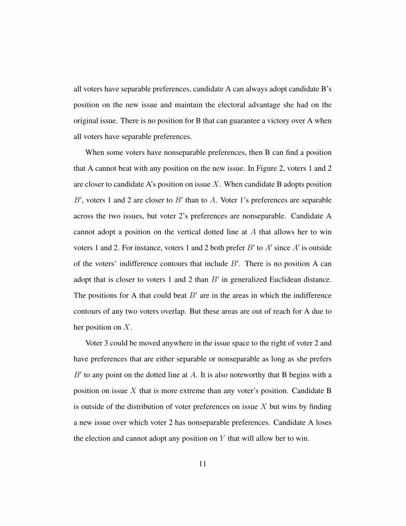
all voters have separable preferences, candidate A can always adopt candidate B’s

position on the new issue and maintain the electoral advantage she had on the

original issue. There is no position for B that can guarantee a victory over A when

all voters have separable preferences.

When some voters have nonseparable preferences, then B can find a position

that A cannot beat with any position on the new issue. In Figure 2, voters 1 and 2

are closer to candidate A’s position on issueX . When candidate B adopts position

B′, voters 1 and 2 are closer to B′ than to A. Voter 1’s preferences are separable

across the two issues, but voter 2’s preferences are nonseparable. Candidate A

cannot adopt a position on the vertical dotted line at A that allows her to win

voters 1 and 2. For instance, voters 1 and 2 both prefer B′ to A′ since A′ is outside

of the voters’ indifference contours that include B′. There is no position A can

adopt that is closer to voters 1 and 2 than B′ in generalized Euclidean distance.

The positions for A that could beat B′ are in the areas in which the indifference

contours of any two voters overlap. But these areas are out of reach for A due to

her position on X .

Voter 3 could be moved anywhere in the issue space to the right of voter 2 and

have preferences that are either separable or nonseparable as long as she prefers

B′ to any point on the dotted line at A. It is also noteworthy that B begins with a

position on issue X that is more extreme than any voter’s position. Candidate B

is outside of the distribution of voter preferences on issue X but wins by finding

a new issue over which voter 2 has nonseparable preferences. Candidate A loses

the election and cannot adopt any position on Y that will allow her to win.

11

The example does not require that the median voter have nonseparable pref-

erences. Similar examples are possible when a moderate voter 2 has separable

preferences while a more extreme voter 1 has nonseparable preferences. Candi-

date A does not have to be located at the position of the median voter onX as long

as she is closer to the median voter than B. Candidate B does not have to adopt

the position of the median voter on issue Y .

Figure 2 illustrates that a candidate can move from a losing position to a win-

ning position by introducing an issue on which voter preferences are nonseparable

from the original issues in the election. Only one of three voters in the example

has nonseparable preferences. There is not a critical number of voters who must

have nonseparable preferences in order for the result to hold. The one pivotal voter

with nonseparable preferences gives candidate B an opportunity to find a winning

position.

Political candidates frequently present voters with packages of issues. Ronald

Reagan in 1980 told American voters that if they agreed with him on any issue

of taxing, spending, national defense, and deficit reduction, then they agreed with

him on the whole set of issues. Bill Clinton and Tony Blair advocated a “Third

Way” of free trade combined with job training and social insurance programs to

aid workers whose jobs disappeared due to globalization. The Republican party

during the 1850s and 1860s quickly rose from a minor party to one of the two ma-

jor parties on a platform of restricting the Westward expansion of slavery while

promoting infrastructure development that would help Western farmers ship their

products to markets in the East. The combination of opposition to slavery and

12

support for internal improvements linked the interests of voters in the East and

West, giving the Republicans a national electoral majority for decades. Candi-

dates’ strategies are made richer by the possibility of exploiting voters’ nonsep-

arable preferences to engineer packages of issues that appeal to voters when the

issues individually might not.

Do Voters Have Nonseparable Preferences?

Are nonseparable preferences a theoretical curiosity or empirical reality? Few

public opinion surveys include questions designed to measure whether voter pref-

erences are nonseparable across issues. Questions designed to detect nonsepara-

ble preferences appeared on a 2004 survey of US citizens.2 The survey contained

questions about twelve different issues that figured prominently in candidate de-

bates and commentary about the election. Although each of the twelve issues

could be nonseparable from all of the remaining issues for some voters, detecting

nonseparable preferences across all combinations of issues would have been im-

possible in a 20-minute survey. To make the survey manageable, questions paired

each issue with only one other issue — some obviously related, some probably

not — to uncover nonseparable preferences. For instance, taxes and education

2Knowledge Networks recruited over 50,000 subjects nationwide to participate in surveys ad-ministered by WebTV. The computer format of the survey allows respondents to complete surveysat their leisure, and often results in more reliable and valid responses than telephone interviews(Chang and Krosnick 2009). A random sample of the Knowledge Networks panel was chosento participate in a three-wave survey, with Wave 1 conducted April 27-May 31 (N=1308); Wave2, September 17-October 7 (N=947); and Wave 3, November 19-December 3, 2004 (N=717). Asample of 211 new respondents also completed interviews in Wave 3. Completion rates were 76percent in Wave 1, 85 percent in Wave 2, and 77 percent in Wave 3.

13

spending were paired. For the issue of taxes, respondents first answered a ques-

tion similar to existing surveys. We label this type of question “unconditional”

since it asks a respondent’s opinion on an issue in isolation, without reference to

the outcome of other issues. Later in the survey respondents answered two “con-

ditional” questions to detect whether preferences on taxes are nonseparable from

spending on education. The questions were:

(unconditional) Do you want the amount of money that people pay in

taxes to the U.S. government to

go up a lot, say to 50% more than we spend now

go up somewhat, say to 25% more than we spend now

go up a little, say to 10% more than we spend now

remain at current levels

go down a little, say to 10% less than we spend now

go down somewhat, say to 25% less than we spend now

go down a lot, say to 50% less than we spend now

(conditional) If the government reduces the amount of money it spends

on education to 25 percent less than it spends now, then would you

want the amount of money that people pay in taxes to the U.S. gov-

ernment to

go up a lot, say to 50% more than we spend now

go up somewhat, say to 25% more than we spend now

go up a little, say to 10% more than we spend now

14

remain at current levels

go down a little, say to 10% less than we spend now

go down somewhat, say to 25% less than we spend now

go down a lot, say to 50% less than we spend now

(conditional) If the government increases the amount of money it

spends on education to 25 percent more than it spends now, then

would you want the amount of money that people pay in taxes to

the U.S. government to

go up a lot, say to 50% more than we spend now

go up somewhat, say to 25% more than we spend now

go up a little, say to 10% more than we spend now

remain at current levels

go down a little, say to 10% less than we spend now

go down somewhat, say to 25% less than we spend now

go down a lot, say to 50% less than we spend now

Similar questions appeared on the survey for education spending conditional on

different levels of taxes. The two conditional questions reveal whether preferences

are separable or nonseparable. In a crosstabulation of responses to the conditional

questions, all responses on the diagonal do not change on the issue of taxes de-

pending on the level of education spending. Responses above the diagonal in-

dicate nonseparable positive complements: a person wants taxes to increase as

education spending increases but wants taxes to decrease as education spending

15

decreases. Responses below the diagonal indicate nonseparable negative com-

plements: as education spending increases, a person wants taxes to decrease; as

education spending decreases, a person wants taxes to increase. In a split-half

sample, some respondents answered the two conditional questions before the un-

conditional question, others answered the questions in reverse order.

While nonseparable preferences should be expected for taxing and spending

issues, many other issues are nonseparable to some people. Respondents answered

questions that paired about defense spending and health care spending, Social

Security and free trade, same sex marriage and same sex adoption, immigration

and a national health insurance plan, and, in wave 2 only, background checks for

gun owners and a ban on assault weapons.

Table 1 shows the percentage of respondents with nonseparable preferences

(both positive and negative complements) for all twelve issues in the survey. The

remaining percentages of responses are separable. The issues are ordered from

the largest to the smallest combined percentage of nonseparable preferences. For

half or more of the issues, at least 20 percent of respondents have nonseparable

preferences. Issues such as immigration and national health care, trade, defense

spending, Medicare spending, and the assault weapons ban all show significant

percentages of potential voters with nonseparable preferences. Recall that even a

small percentage of voters with nonseparable preferences create opportunities for

candidates to package issues strategically.3

3The percentages of respondents with nonseparable preferences for taxes conditional on educa-tion does not have to match the percentage with nonseparable preferences for education spendingconditional on taxes since voters may have partially nonseparable preferences.

16

Table 2 shows the percentage of respondents who have nonseparable prefer-

ences broken down by the voter’s self-placement on a standard seven-point ide-

ological scale. Voters who described themselves as ideological moderates, at the

midpoint of the scale, are more likely to have non separable preferences on most

issues than voters who are more ideologically extreme. This finding suggests that

the example in Figure 2 may not be far off from real elections where voters in the

middle of the issue space are the ones who have nonseparable preferences. In a

one dimensional issue space or a multidimensional space in which all voters have

separable preferences, the ideal points of moderate voters always remain in the

middle of the space. But in a multidimensional space, moderate voters who have

nonseparable preferences may have induced ideal points that make them more

extreme on bundles of issues.

The results may also explain evidence of the disappearing center in electoral

politics. Much has been written about the rise in polarization among voters and

elected officials (Abramowitz 2010). But other evidence suggests that most vot-

ers remain moderate on most issues, and the voter preferences are normally dis-

tributed rather than bimodal (Fiorina 2005). As Figure 2 shows, moderate voters

with nonseparable preferences over issues can have induced ideal points that are

more extreme. Voter 2, for instance, has an ideal point on issue X that makes him

the median voter on X . But when issue Y is introduced, he supports candidate

B’s extreme position on X . Even though voter 2’s ideal point may be moderate

on X , his induced ideal point given the constraints of the options before him –

candidate positions A and B′ – is extreme. Debates about whether voters are ex-

17

treme or moderate, polarized or centrist, are based on interpreting the distribution

of voter ideal points issue by issue (Fiorina 2005, Abramowitz 2010). We need

more information about voter preferences across issues to draw conclusions about

whether voters are moderate or extreme. Nonseparable preferences may make

moderate voters appear extremist or extremist voters appear moderate depending

on the constraints imposed by other issues or the candidates’ positions.

Conclusion

As E. E. Schattschneider wrote, “Political strategy deals ... with the inclusion

and exclusion of contestants because it is never true that the balance remains the

same if the number is changed” (1957:941). The same may be said of political

issues as contestants. Changing the issues can tip the balance of a close election.

We already know that moving from one issue to multiple issues fundamentally

alters the nature of elections. As we show in this chapter, moving to a multi-

dimensional issue space can be a strategic choice in an election. Introducing new

issues may be a candidate’s only hope of unseating an entrenched opponent. But

simply introducing a new issue is not alone a path to victory. For a disadvantaged

candidate to have any hope of winning an election by introducing new issues,

some voters must see the issues as linked.

In the one dimensional spatial model, two competing candidates will converge

to the position of the median voter. This theoretical result does not fit reality, pri-

marily because politics is multidimensional. In a multidimensional model with

18

two candidates, an equilibrium will not generally exist and candidates will change

positions on issues in a never-ending quest for an electoral advantage. This predic-

tion also does not appear to fit real elections. Imposing some additional realistic

structure on the multidimensional spatial model of electoral competition produces

new and surprising results.

When candidates have fixed positions in an issue space, a candidate can take

a position on a new issue in order to beat an advantaged opponent. Instead of

changing positions on existing issues, a potentially costly strategy if voters penal-

ize “flip-floppers,” candidates can compete by expanding the scope of conflict to

include new issues. But only when some voters have nonseparable preferences

will the strategy of introducing a new issue prove beneficial for a disadvantaged

candidate. Issue packaging is a fundamental strategy of electoral politics, part

of what William Riker called “heresthetics,” or the art of political manipulation

(Riker 1986).

19

References

Abramowitz, Alan. 2010. The Disappearing Center: Engaged Citizens, Po-

larization, and American Democracy. New Haven: Yale University Press.

Aldrich, John H. 1983. “A Downsian Spatial Model with Party Activism.”

American Political Science Review 77(4):974-990.

Black, Duncan. 1957. “On the Rationale of Group Decision-Making.” Jour-

nal of Political Economy 56:23-24.

Black, Duncan, and R.A. Newing. 1951. Committee Decisions with Comple-

mentary Valuation. London: William Hodge and Company.

Chang, LinChiat., and John A. Krosnick. 2009. “National Surveys Via RDD

Telephone Interviewing Versus the Internet: Comparing Sample Representative-

ness and Response Quality.” Public Opinion Quarterly 73(4):641-678.

Davis, Otto A., Morris H. DeGroot, and Melvin J. Hinich. 1972. “Social

Preference Orderings and Majority Rule.” Econometrica 40(1, January):147-157.

Davis, Otto A., Melvin J. Hinich, and Peter C. Ordeshook. 1970. “Social

Preference Orderings and Majority Rule.” American Polititical Science Review

64(2, June):426-448.

Downs, Anthony. 1957. An Economic Theory of Democracy. New York:

Harper and Row.

Enelow, James M., and Melvin J. Hinich. 1983. “Voting One Issue at a Time:

The Question of Voter Forecasts.” American Political Science Review 77(June):

435-445.

20

Enelow, James M., and Melvin J. Hinich. 1984. The Spatial Theory of Voting:

An Introduction. New York: Cambridge University Press.

Fiorina, Morris P. 2005. Culture War? The Myth of a Polarized America. New

York: Longman.

Hotelling, Harold. 1929. “Stability in Competition.” The Economic Journal

39:41-57.

Kadane, Joseph. 1972. “On Division of the Question.” Public Choice 13:47-

54.

Kramer, Gerald H. 1972. “Sophisticated Voting Over Multidimensional Choice

Spaces.” Journal of Mathematical Sociology 2:165-80.

Lacy, Dean, and Emerson M. S. Niou. 2000. “A Problem with Referendums.”

Journal of Theoretical Politics 12(1, January):5-31.

Lacy, Dean. 2001. “A Theory of Nonseparable Preferences in Survey Re-

sponses.” American Journal of Political Science 45(2, January):239-58.

McKelvey, Richard D. 1976. “Intransitivities in Multidimensional Voting

Models and Some Implications for Agenda Control.” Journal of Economic Theory

12:472-82.

Petrocik, John R.. 1996. “Issue Ownership in Presidential Elections, with a

1980 Case Study.” American Journal of Political Science 40(3):825-50.

Plott, Charles R. 1976. “Axiomatic Social Choice Theory.” American Journal

of Political Science 20(3):511-596.

Riker, William H. 1982. Liberalism Against Populism: A Confrontation Be-

tween the Theory of Democracy and the Theory of Social Choice. Waveland.

21

Riker, William H. 1986. The Art of Political Manipulation. New Haven: Yale

University Press.

Schattschneider, E. E. 1957. Intensity, Visibility, Direction, and Scope. Amer-

ican Political Science Review 51(4, December):933-942.

Schattschneider, E. E. 1960. The Semisovereign People. New York: Holt,

Rinehart, and Winston.

Schofield, Norman. 1978. Instability of Simple Dynamic Games. The Review

of Economic Studies 45(3)):575-594.

Schwartz, Thomas. 1977. “Collective Choice, Separation of Issues and Vote

Trading.” American Political Science Review 71:999-1010.

22

Figure 1: All Voters Have Separable Preferences

A B

1

3

2

Y

X

B’ A’

z1 z2 z3

z’2 z’1 z’3

Voters 1 and 2 are closer to Candidate A’s position; voter 3 is closer to CandidateB’s position. After B moves to B′, A can find another position, A′, that maintainsher advantage on the distribution of induced ideal points, z′i.

23

Figure 2: A Pivotal Voter Has Nonseparable Preferences

A B

1

3

2

Y

X

B’

A’

Voters 1 and 2 are closer to A than to B on issue X . Voters 1 and 2 switch tosupporting candidate B after she moves to B′. Candidate A cannot find a positionon issue Y to win back both voters 1 and 2 given her position on issue X .

24

Table 1: Percentages of Respondents with Nonseparable Preferences

Positive NegativeIssue Conditional On N Complements Complements

May 2004, N=735

Taxes Education spending 623 46.7% 7.2%

Education spending Taxes 620 42.2 8.2

Medicare spending Defense spending 621 18.5 17.6

Defense spending Medicare spending 622 12.2 22.3

National health care Immigration 622 2.25 15.8

Free Trade Privatize Social Security 623 14.8 8.7

Assault weapons ban Background checks 448* 4.2 9.5

Immigration National health care 628 8.6 16.2

Privatize Social Security Free Trade 617 6.3 3.6

Adoption Marriage 626 6.8 2.1

Marriage Adoption 621 3.8 0.8

Background Checks Assault weapons ban 451* 1.6 1.6

Source: 2004 Panel Survey of Nonseparable Preferences. * indicates questions from wave 2, N=462.

25

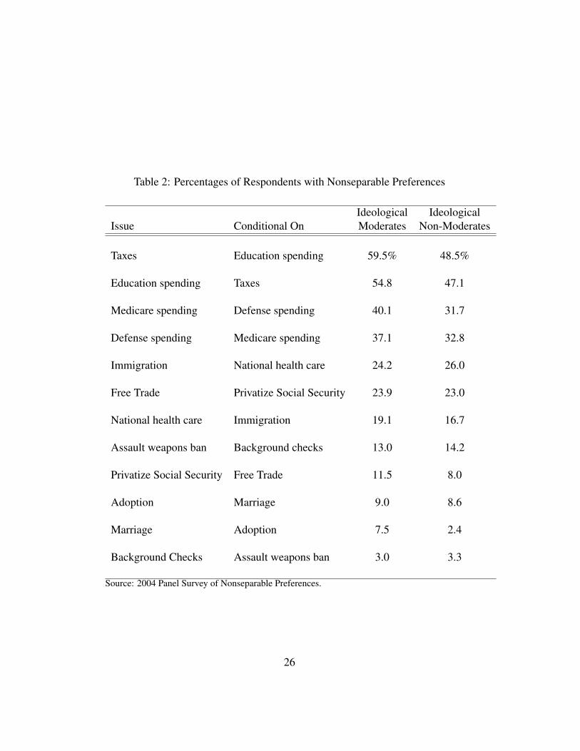
Table 2: Percentages of Respondents with Nonseparable Preferences

Ideological IdeologicalIssue Conditional On Moderates Non-Moderates

Taxes Education spending 59.5% 48.5%

Education spending Taxes 54.8 47.1

Medicare spending Defense spending 40.1 31.7

Defense spending Medicare spending 37.1 32.8

Immigration National health care 24.2 26.0

Free Trade Privatize Social Security 23.9 23.0

National health care Immigration 19.1 16.7

Assault weapons ban Background checks 13.0 14.2

Privatize Social Security Free Trade 11.5 8.0

Adoption Marriage 9.0 8.6

Marriage Adoption 7.5 2.4

Background Checks Assault weapons ban 3.0 3.3

Source: 2004 Panel Survey of Nonseparable Preferences.

26

When will insider candidates avoid a primary

challenge? A model of partial revelation of information

Gilles Serra∗

1 Introduction

Incumbents and other insiders tend to enjoy a comfortable position within their parties. In

particular, they frequently have an advantage to secure their party’s nomination for a future

election. Outsiders who do not necessarily belong to the dominant faction in the party

have a much harder time getting their name on the ballot. They are disadvantaged in at

least two ways: they might be less well-known than the party grandees they are competing

with; and there might not even be a fair competition such as a primary election for them

to prove themselves. A question of interest is why parties allow well-known insiders to have

such and advantage over lesser-known outsiders. We would imagine an ambitious party that

wishes to win elections to find mechanisms for identifying and selecting the best possible

candidate, regardless of that candidate’s previous standing in the party. One option would

be to democratize the nomination process to let fresh outsiders join an open competition

where they can display their true campaigning skills. This option is widely available to

political parties around the world, though it is not always used. In this paper I explore the

conditions under which candidate-selection is democratized, and I show that rational parties

who wish to find the most talented candidate may nevertheless shut down the possibility of

unknown hopefuls coming forward to display their talents.

∗Department of Political Science, Center for Economics Research and Teaching (CIDE), Mexico City,Mexico, gilles.serra@cide.edu

1

Indeed, a political party can use a variety of methods to nominate those who will later

compete for office at a given election. Broadly speaking, a candidate-selection method (CSM)

can fall in two categories. On one hand, the method could be open (or democratic) by al-

lowing the participation of all the members, activists and sympathizers of the party in the

nomination of candidates. Of all the selection methods that parties can use, the most open

and democratic one is the primary election. By primary election, I refer to the organized

competition among aspiring candidates within the same party that culminates in the de-

mocratic vote of all party members. On the other hand, the nomination method could be

closed (or undemocratic), consisting of a closed-door decision at the elite level of the party.

For example, the nominee for an upcoming presidential or gubernatorial election could be

chosen by a handful of party bosses at a private meeting. As argued throughout this paper,

the choice matters for the party in terms of its prospects of winning the election; but it also

matters for citizens in terms of the quality of candidates they are offered.

Party leaders are for the most part responsible for the way their parties nominate can-

didates. In most presidential systems, political parties have leeway in choosing their CSM,

and it is usually not the case that primaries are exogenously imposed on them by the gov-

ernment. In fact, it is common for political parties to have serious deliberations on what

CSM to adopt before even discussing which candidates to select. Their adoption of primary

elections is most often voluntary rather than mandated by law. Throughout Latin Amer-

ica we repeatedly see party elites debating whether to open the nomination process or not.

Actually, it is not uncommon for parties to go back and forth between primaries and other

CSMs in recurrent elections, which clearly indicates the strategic nature of that choice. In

the United States, party elites also have a strong say in choosing wether their nomination will

be open and inclusive, or closed and exclusive. They do so by choosing whether to endorse a

favored candidate or not. If party leaders decide to rally behind a well-known insider, they

will provide her with public endorsements, strategic advice and large amounts of funding to

overwhelm any challenger. On the other hand, if party leaders do not identify an insider

candidate that satisfies them, they will withhold or divide their endorsements such that a

competitive race among several hopefuls takes place. Thus, while parties are "officially"

2

holding a primary election, in practice that primary can be competitive or uncompetitive.

In effect, this is equivalent to choosing between a democratic and an undemocratic CSM.

Hence, I claim the explanation for the use of primaries around the world lies in the strategic

calculations of party leaders

This paper postulates a benefit to party leaders that helps explain why they occasionally

allow the use of primary elections within their parties. To be concrete, I claim that primary

elections have a practical advantage over elite-centered nominations: they reveal information

about candidates’ appeal to voters. My premise is that a candidate nominated through a

primary election can be expected to have higher campaigning skills than a candidate nom-

inated through an elite appointment. This happens because the primary campaigns reveal

valuable information about the contenders. Indeed, there is much uncertainty surrounding

the individuals seeking to become a party’s candidate, often called pre-candidates. Their

future vote-getting effectiveness is never known for sure. A primary can serve as a "trial"

election within a party that shares many of the features of the subsequent general election

between the parties. Pre-candidates must participate in debates, broadcast television ad-

vertisements, manage a campaign, and so forth. Thus primaries can reveal how effective

the pre-candidates would be in the general election. In that sense, my model provides an

"information rationale" for the existence of primary elections.

On the other hand, as mentioned above, primaries might carry several costs to party

leaders. In this paper I focus on one oft-mentioned cost: primary elections might push

candidates to adopt policies far from the leaders’ preferences. Indeed, the party bosses know

that primary voters may not quite share their ideology. They might be too extremist or

too moderate to be trusted with the selection of the party’s candidate. The main point is

that party leaders face a trade-off between the costs and benefits of a primary election. The

results in this paper reveal that the party leaders’ decision is not trivial

On that basis, I build a spatial voting model that includes a party’s choice between a

competitive primary election and an elite-centered nomination. The main question is: When

does the informational benefit of primaries outweigh the cost of losing control of the candi-

dates’ platforms? As the results will indicate, the answer depends on several fundamental

3

variables: the ideology of parties, the ideology of primary voters, the intensity of the primary

election, and the quality of insider and outsider candidates.

This model is a continuation of the research in Serra (2011). The main contribution

with respect to that research is analyzing the revelation of partial information rather than

full information, by which I mean that primary elections only reveal part of the information

needed to assess a contender, but his or her ability to perform well in the general election

would still not be known in full. To be concrete, I assume the contenders’ performances

within the party are interpreted as "noisy signals" that can be interpreted as forecasts of

their performance if they were nominated to compete against another party. In this sense,

the model falls in the tradition of modeling voting as a process to aggregate information—a

tradition initiated by Condorcet(1785), Austen-Smith and Banks (1996), and Feddersen and

Pesendorfer (1998).

Several new results are found with this modeling choice. Two new variables can be

studied more precisely. The ability of primaries to reveal valuable information, which I call

the quality of primaries; and the reputation of the insider candidate as proficient vote-getter,

which I call the prior belief about the insider’s skill. Regarding the quality of primaries,

I find that a party can benefit from stiff competition in its primary election. This result

stands in contrast with an oft-mentioned view that parties should ensure their primaries are

light and cordial. Regarding the prior belief held about the skill of candidates, I find that an

insider might have a good enough reputation to prevent a primary election altogether. This

result would help explain why many incumbents are able to be re-nominated for a subsequent

election without being opposed inside their parties. Both results are new in the literature

on primary elections as far as I can tell.

In addition to these new results, many of the previous results in Serra (2011) are cor-

roborated. In particular, this paper also finds that primaries are more likely when there is

congruence between the elite and the mass membership of the party; and primaries are more

appealing to the party that is most disadvantaged given its valence and policies.

The rest of the paper is developed as follows: Section 2 briefly summarizes the theoretical

literature that relates to my model. Section 3 introduces a spatial voting model between

4

two parties that will serve to study the general election. It is a variant of the Downsian

voting model, with an additional dimension corresponding to the candidates’ valence. In

Section 4, I take a step back in the electoral process, and I study the nomination that takes

place inside a party before the general election. Section 5 develops a signaling mechanism for

primary voters to update their beliefs about pre-candidates based on their performance in

the primary campaigns. Section 6 introduces a cost of adopting primaries based on the lack

of congruence between the elite and the mass in the party. In Section 7, I derive a number

of conditions for a party to hold a competitive primary election, which is the purpose of this

paper. Finally, Section 8 discusses the main results and suggests some interpretations of

relevance to democratic theory. The appendix contains all the proofs of the results in this

paper.

2 Previous theories of the adoption of primary elec-

tions

The paper adds to the formal literature on primary elections. Most authors have studied

the consequences of primaries, rather than their causes. Several papers in that literature

share common aspects with this one, especially those comparing different candidate-selection

methods (CSM). Owen and Grofman (2006) compare primaries with different degrees of

divergence between the party mean and the population mean. Jackson, Mathevet andMattes

(2007) study three different nomination processes: an arbitrary appointment by a party

leader, a primary election, and a spending competition between candidates. In Castanheira,

Crutzen, and Sahuguet (2008), parties select their internal organization possibly including

intra-party competition. Cho and Kang (2008) compare open and closed primary elections.

Another set of papers that relate to my model, are those that have paid attention to

informational aspects of primaries. In Caillaud and Tirole (1999), the use of primaries

provides information about the credibility of the party. In Meirowitz (2005), primaries allow

candidates to acquire information about voters’ preferences. Then there is a set of papers

where primaries reveal information about the valence of primary contenders.

5

For instance, Adams and Merrill (2008) postulate that primary elections may allow a

party to identify a high-quality nominee. The authors find, as I do, that weak parties benefit

from primaries more than strong parties do. In spite of those similarities, our models have

important differences because the focus of their paper is the candidates’ choice of platforms,

while the focus of my paper is the parties’ choice of candidates.

Another closely related paper is Snyder and Ting (2011) who also studies a party’s

decision to hold a primary election or not. As in my model, parties compete both in terms

of ideology and valence. Snyder and Ting also assume that primaries increase the expected

valence of the nominee. A main difference is the alternative CSM. If a party does not hold a

primary, Snyder and Ting assume that the nominee will be chosen at random among all the

willing precandidates. In contrast, I assume the party elite will choose an insider candidate

in a smoke-filled room. Another difference is that both parties are bound to use the same

CSM by state law, whereas in my model parties can have different CSMs.

Kselman (2012) develops a model where aspirants must compete in a primary election

to obtain their party’s nomination. In his model, candidates enjoy a type of valence that

serves as a bonus for parties that are office-seeking. Interestingly, this type of valence is

particularistic in the sense that only a subset of voters benefit from it.

Finally, this paper is related to the literature on endogenous valence. Some other papers

have also allowed the agents in their models to affect the valence parameter are Ashworth

and Bueno de Mesquita (2007), Schofield and Sened (2005), Schofield (2007), Carrillo and

Castanheira (2008) and Callander (2008), Meirowitz (2008), Schofield, Claassen, Ozdemir,

Schnidman and Zakharov (2008).

The model in this paper is one of the few that combines both literatures, the one on

valence and the one on primaries. As in Adams and Merrill (2008), Snyder and Ting (2011),

and Serra (2011), the premise here is that primaries help parties by revealing the valence of

their candidates. Unlike those papers, however, this paper develops a signaling mechanism

to reveal partial rather than full information. As a consequence, I consider the possibility

that information is not revealed fully but only partially.

6

3 General election between the two parties

In this section I focus on the competition between two parties without any reference to

primary elections. In essence, this corresponds to the "general election" that occurs after all

parties have already completed their nomination cycle. This will be a valence-policy model,

meaning that it will have two dimensions. First, the election occurs in a left-right policy

spectrum. I denote by x the policy implemented, with x ∈ R. Second, there is a dimensioncorresponding to valence, which is described in detail below. The valence dimension is

denoted by v, with v ∈ R+. The model I present here is an application of the more generalmodel developed in Serra (2010).

3.1 Parties

There are two parties competing in this election, labeled party L and party R. Following

the Wittman-Calvert-Roemer tradition, I assume that parties are policy-motivated, meaning

that they care about the policy implemented after the election (Wittman 1973, Calvert

1985, Roemer 2001). Parties L and R have ideal policy points XL and XR, respectively.

The two parties have distinct ideologies so that XL 6= XR. I normalize the ideal point of themedian voter in the general election to zero, and without much loss of generality I assume

XL < 0 < XR. The utility functions of L and R are

UR (x) = − |XR − x|

UL (x) = − |XL − x|

In later sections I will specify two separate groups within party R with different ideal points

XRE and XRM . For this section, however, it is sufficient to think of XR as the generic ideal

point of R. At this stage it is useful to define a few concepts. By a party’s extremism I will

mean how far it’s ideal point is from the median voter’s ideal point. Concretely, party R’s

extremism will be measured by |XR|, and party L’s extremism will be measured by |XL| .11Of course, note that |XR| = XR and |XL| = −XL.

7

Finally, parties formulate policy platforms to compete in the election, and they do so

strategically in order to maximize their expected utility. I call those platforms xL and xR,

with xL, xR ∈ R.

3.2 Candidates

All candidates are characterized by a parameter v denoting how appealing their non-policy

attributes are to voters in that election. Parameters such as v have been called "valence

parameters" and can be given many interpretations (for an overview see Schofield (2007) and

Adams, Merrill, Stone and Simas (2009)). In the context of this paper, v is best interpreted

as the candidate’s campaigning skill. It can take two values: a low value normalized to zero

corresponding to a low-skilled candidate, and a high value of V corresponding to a high-

skilled candidate. Hence v ∈ {0, V } . I label vL and vR the skills of candidates in parties LandR, respectively. To focus on the interesting cases, I will assume that valence is sufficiently

salient to make a difference in the election; technically I will assume that the valence of a

high-skilled candidate is strictly larger than the extremism of both parties, meaning that

|XL|, |XR| < V. 2 Indeed, for smaller values of V , the valence dimension loses influence inthe election and the results become trivial. I report these results in footnotes, and I refer

the reader to Serra (2011) for a fuller analysis of a lower salience of valence.

In this model, candidates do not have policy preferences of their own. Rather, they will

adopt the policy preferences of their party. To be exact, the candidate will behave as if

having the exact utility function of the party that nominated her. She will announce the

platform designed by her party during the campaigns, and she will implement such platform

in case she wins the election.

3.3 The general electorate

The electorate cares about the policy implemented after the election. To simplify the analy-

sis, I will assume that there is a median voter, which I callM, whose preferences are decisive

in the election. I normalize her ideal point to zero.

2This is equivalent to assuming that −V < XL and XR < V.

8

In addition to the policy implemented x, the electorate also cares about the skill v of the

winning candidate. The utility function of M is given by

UM (x, v) = − |x|+ v

M will vote for the party whose candidate maximizes her utility. I make the following

indifference assumptions. If M is indifferent between the two parties, she will vote for the

one whose candidate has the highest skill. If both candidates have the same skill, she will

randomize equally between the two.

Figure 1: The effect of a valence advantage for R over L

It is worth looking more closely at how the median voter makes her decision in this kind

of model. As elaborated in Serra (2010), M ’s appreciation for a candidate decreases with

the distance between her ideal point and that candidate’s platform, and increases with the

candidate’s valence. In essence, the valence parameter v "shifts up" the utility function of

M. An example of how M evaluates R and L is illustrated in Figure 1, where it is assumed

that vL < vR and |xL| < |xR|. In the case depicted in this figure, candidate R is strictly

preferred to candidate L in spite of having a more extremist platform. Candidate R is able

to win the election because her higher score in the valence dimension more than compensates

9

her extremism in the policy dimension.

3.4 Timing and solution concept

The timing of this election is the following:

1. Assessment of the candidates’ skills: Parties announce their candidates who start

campaigning. The candidates’ campaigning skills vL and vR are observed.

2. Assessment of the policy platforms: Candidates announce their platforms xL and

xR.

3. The general-election vote: The median voter elects L or R.

Stage 1 does not involve any decision: the candidates are revealed to voters, along with

their valence attributes. The first decision is made in Stage 2 where each candidate must

announce and promote her platform taking the other candidate’s platform into account.

In Stage 3, once candidates’ skills, vL, vR, and platforms, xL, xR, have been observed and

assessed, the median voter elects L or R to office. All this information is common knowledge.

The game must be solved by backward induction and the solution concept is subgame-perfect

equilibrium (SPE) in pure strategies. It will be important to recall that a SPE requires that

all strategies form a Nash equilibrium (NE) in every subgame.

3.5 Results of the general election

Before stating the main results of this section, some important variables should be defined.

I call ∆v the difference in skill between R’s candidate and L’s candidate. To be concrete,

∆v ≡ vR − vL. Note that ∆v can take three values: ∆v ∈ {−V, 0, V } . I call x∗L and x∗R theequilibrium strategies of parties L and R, and x∗ the winning platform. These parameters

will determine the results of the general election, as indicated in the main theorem on this

section. It must be remember that valence was assumed to be salient enough that |XL| and|XR| are smaller than V , which implies that −V < XL and XR < V.

10

Theorem 1 The equilibrium strategies and equilibrium outcomes of this election for given

values of vL, vR, V,XL and XR are given in the following table, where ∆v ≡ vR − vL.

Table 1: Equilibrium outcomes of the general election

Value Equilibrium platforms Winning platform Winning

of ∆v x∗R and x∗L x∗ party

V x∗R = XR XR R

x∗L ∈ R0 x∗R = 0 0 R or L with

x∗L = 0 equal probability

−V x∗R ∈ R XL L

x∗L = XL

There are several comments to make about this table.3 First note the results when

∆v = 0, that is, when there is no skill difference between the candidates. Both parties

converge completely to the median voter’s ideal point. However, when ∆v 6= 0 the candidatewith highest skill is able to diverge from the median voter toward the ideal point of her party,

and still win the election based on her superior skill. So the policy implemented is biased

toward R when ∆v > 0, biased toward L when ∆v < 0, and unbiased when ∆v = 0. In

fact, given the assumption that valence is salient enough, the party with the highest-skilled

candidate is able to pull policy all the way to its ideal point.4 Such equilibrium is illustrated

in the figure below, which depicts the case where 0 < XR < ∆v.

3The proofs of all the results come in the appendix.4This ideal point depends on which group controls policy within the party. In this section we have called

XL and XR the generic ideal points of parties L and R. In later sections, however, party R’s ideal point willbe given by XR = XRE if the leaders control policy, or XR = XRM if the members control policy. In otherwords, what we mean by "party" will vary according to the CSM.

11

Figure 2: Equilibrium platforms x∗L and x∗R

when there is a valence advantage for R over L

4 The nomination process

In this section, I take a step back in the election process to study the nomination of candi-

dates within a party. At this stage, the identity of each party’s candidate is still unknown.

Consequently, the exact values of the candidates’ campaigning skills are uncertain. However,

there exist some prior beliefs about these skills based on some information about parties and

their potential candidates. According to that information, the probabilities that L’s candi-

date and R’s candidate will be high-skilled are πL and πR respectively, with πL,πR ∈ (0, 1) .In other words, πL ≡ P (vL = V ) and πR ≡ P (vR = V ) . Those prior beliefs before the

election campaigns are common knowledge among voters and parties.

The rest of this paper seeks to study the ability of party R to increase πR by choosing

a CSM over another. Indeed, choosing to hold a primary election could affect πR positively

under circumstances specified below. There could be a cost, however, in terms of the policy

implemented by the candidate after a primary. Solving party R’s cost-benefit analysis is the

final goal of this research. I eschew in this paper the parallel decision of party L whom might

also be pondering whether to choose a primary election. Such analysis is being done in a

12

separate paper, and here I simply assume that party L has already chosen a candidate by

any method. In other words, πL is taken as an exogenous parameter. In any case, remember

that the actual campaigning skills of L and R’s candidates are revealed when they start

campaigning to win the election. Thus vL and vR are fully known when voters decide who

to vote for.

4.1 Party members versus party leaders

Party R consists of an "elite" (or "leadership") and a "membership" (or "rank and file").

The elite of R will be referred to as RE. This leadership is policy-motivated and has an ideal

policy point XRE, with XRE > 0. The utility function of R’s elite is

URE (x) = − |XRE − x|

The rank and file (RAF) of R is also policy-motivated. To simplify the analysis, I will

assume that the RAF has a median member whose preferences are decisive in the primary

election. I call RM the median member of R and I call XRM her ideal point, with XRM > 0.

The utility function of RM is

URM (x) = − |XRM − x|

In general, we will have XRE 6= XRM , so there will be a tension between the policy prefer-ences of a party’s leadership and its RAF. It will be useful to measure the divergence, if any,

between a party’s establishment and its primary voters. With that purpose, I define dR as

the internal divergence in party R, where dR ≡ |XRM −XRE| . An interesting interpretationof dR is as the congruence (or lack thereof) between R’s elite and mass membership. Higher

levels of the internal divergence dR indicate a lower elite-mass congruence inside the party.

Note that dR can take any non-negative value: dR ≥ 0.Parties are also responsible for formulating policy platforms to compete in the election.

More precisely, parties are in charge of indicating the policy platforms they wish their candi-

13

dates to follow in each circumstance. If party R uses a leadership selection, then its leaders

formulate the policy strategies to be followed by its candidate. If, instead, party R uses a

primary election, then its candidate will follow the policy strategies desired by the RAF. Note

that both the leadership and the RAF think strategically. This implies that they would not

passively impose their ideal points on the candidate, but rather, they will design a strategy

that maximizes their expected utility taking into account the behavior of the rival party in

the general election.

4.2 Primary election versus elite endorsement

Before selecting a candidate, the leadership of party R needs to choose a candidate-selection

method (CSM). There exist two methods: an elite endorsement or a primary election. The

default CSMwould be for the leadership to directly nominate or endorse an insider candidate.

Alternatively, it could hold a competitive primary election where an outsider candidate has

a chance to run, and the decision to choose the nominee is delegated to the party’s rank and

file. I call mR the method that R’s leaders choose, with mR ∈ {elite, primary}. Followingstandard language in the party-politics literature, I will call selectorate the group in charge

of selecting a party’s candidate. If mR = elite, the selectorate is the party’s leadership. If

mR = primary, the selectorate is the party’s RAF. In the former case, XR = XRE. In the

latter case, XR = XRM .

Candidates adopt the policy preferences of their selectorate. In other words, they be-

have as perfect agents of whichever group inside their party nominated them. Therefore,

depending on whether the CSM is a primary election or an elite endorsement, the nominee

will inherit the preferences of either RM or RE, respectively. This is summarized in the

following table:

Table 2: The objective of party R’s candidate

After an elite selection: maxxR URE (x) = − |XRE − x|After a primary election: maxxR URM (x) = − |XRM − x|

14

The interpretation is that in striving to win the nomination, the pre-candidates are forced

to cater to the wishes of those selecting them. In exchange for having their names on the

ticket, they have to yield on policy by making concrete commitments to those in charge

if the nomination. Those commitments are credible because parties have effective ways of

enforcing their candidates’ promises.

4.3 Insiders versus outsiders

An important difference across nomination rules is the number of aspirants who have a

realistic chance of getting their party’s nomination. When a party elite chooses to endorse

someone without further consultation, it is usually because there is a trusted insider who

has previously emerged as the natural nominee. In contrast, when a party decides to allow

a truly competitive primary election, it is opening the door to outside aspirants who might

have previously been unknown or ignored. This empirical observation motivates the following

assumptions.

Any individual who is officially contesting the party’s nomination will be referred to as a

pre-candidate. If mR = elite then party R has only one pre-candidate to choose from, which

I call the insider and I denote by RI. If mR = primary then party R has two pre-candidates

to choose from, which consist of the insider, RI, and an outsider denoted by RO. Hence, by

adopting a primary, the party is expanding the pool of candidates that it can choose from.

I call vRI and vRO the campaigning skills of RI and RO respectively, and I call vR the

campaigning skill of the candidate who is finally nominated by R. As I mentioned before, a

candidate’s skill can take two values, 0 or V. However, the exact values of the pre-candidates’

campaigning skills are uncertain ex-ante. The party has some prior information about the

probability that its insider candidate, RI, is high-skilled or low-skilled. That information

could come from previous performance in office, from past elections, or from polls. According

to that information, RI has a probability πRI of being high-skilled, with πRI ∈ (0, 1) . Onthe other hand, the party has no prior information about the outsider candidate. The party

believes that the outsider candidate RO has a probability of one-half of being high-skilled,

hence πRO = 12.

15

4.4 Timing

The timing of the nomination is the following:

1. The selection of the candidate-selection method: The leaders of party R choose

a nomination process.

2. The nomination contest: If the CSM is a primary election, the pre-candidates

commit to pursuing the policy interests of RM and some information about their skills

is revealed. If the CSM is an elite endorsement, the pre-candidates commit to pursuing

the policy interests of RE and no information is revealed.

3. The nomination decision: Party R selects its candidate.

After this nomination, the game is played exactly as described in the previous section, i.e.

the three stages of the nomination are followed by the three stages of the general election.

All this information is common knowledge.

5 The benefit of primary elections

In this section, I develop a model of primary elections as a means to acquire some information

about the campaigning skills of aspirants. Primaries reveal partial information through a

system of noisy signals sent by candidates and processed by primary voters using Bayes

rule. This informational mechanism is the main innovation with respect to Adams and

Merrill (2008), Serra (2011), Snyder and Ting (2011) and other models postulating that

primaries reveal information about candidates. In those models information is fully revealed

in the primary election, and there is no additional information in the general election. In

contrast, in this model the information is only partially revealed in the primary, and there is

additional information in the general election. As I will show, this realistic assumption leads

to new insights about the adoption of primary elections, in particular the possibility that a

high-skilled insider might prevent such primaries.

16

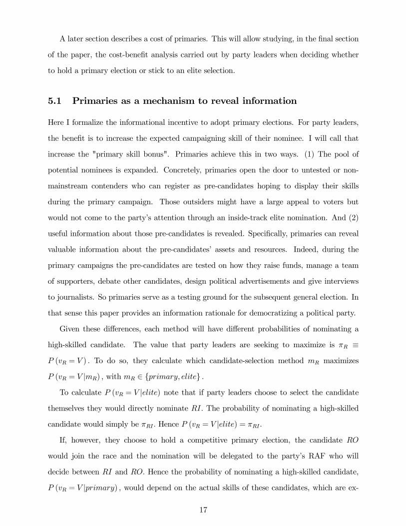
A later section describes a cost of primaries. This will allow studying, in the final section

of the paper, the cost-benefit analysis carried out by party leaders when deciding whether

to hold a primary election or stick to an elite selection.

5.1 Primaries as a mechanism to reveal information

Here I formalize the informational incentive to adopt primary elections. For party leaders,

the benefit is to increase the expected campaigning skill of their nominee. I will call that

increase the "primary skill bonus". Primaries achieve this in two ways. (1) The pool of

potential nominees is expanded. Concretely, primaries open the door to untested or non-

mainstream contenders who can register as pre-candidates hoping to display their skills

during the primary campaign. Those outsiders might have a large appeal to voters but

would not come to the party’s attention through an inside-track elite nomination. And (2)

useful information about those pre-candidates is revealed. Specifically, primaries can reveal

valuable information about the pre-candidates’ assets and resources. Indeed, during the

primary campaigns the pre-candidates are tested on how they raise funds, manage a team

of supporters, debate other candidates, design political advertisements and give interviews

to journalists. So primaries serve as a testing ground for the subsequent general election. In

that sense this paper provides an information rationale for democratizing a political party.

Given these differences, each method will have different probabilities of nominating a

high-skilled candidate. The value that party leaders are seeking to maximize is πR ≡P (vR = V ) . To do so, they calculate which candidate-selection method mR maximizes

P (vR = V |mR) , with mR ∈ {primary, elite} .To calculate P (vR = V |elite) note that if party leaders choose to select the candidate

themselves they would directly nominate RI. The probability of nominating a high-skilled

candidate would simply be πRI . Hence P (vR = V |elite) = πRI .

If, however, they choose to hold a competitive primary election, the candidate RO

would join the race and the nomination will be delegated to the party’s RAF who will

decide between RI and RO. Hence the probability of nominating a high-skilled candidate,

P (vR = V |primary) , would depend on the actual skills of these candidates, which are ex-

17

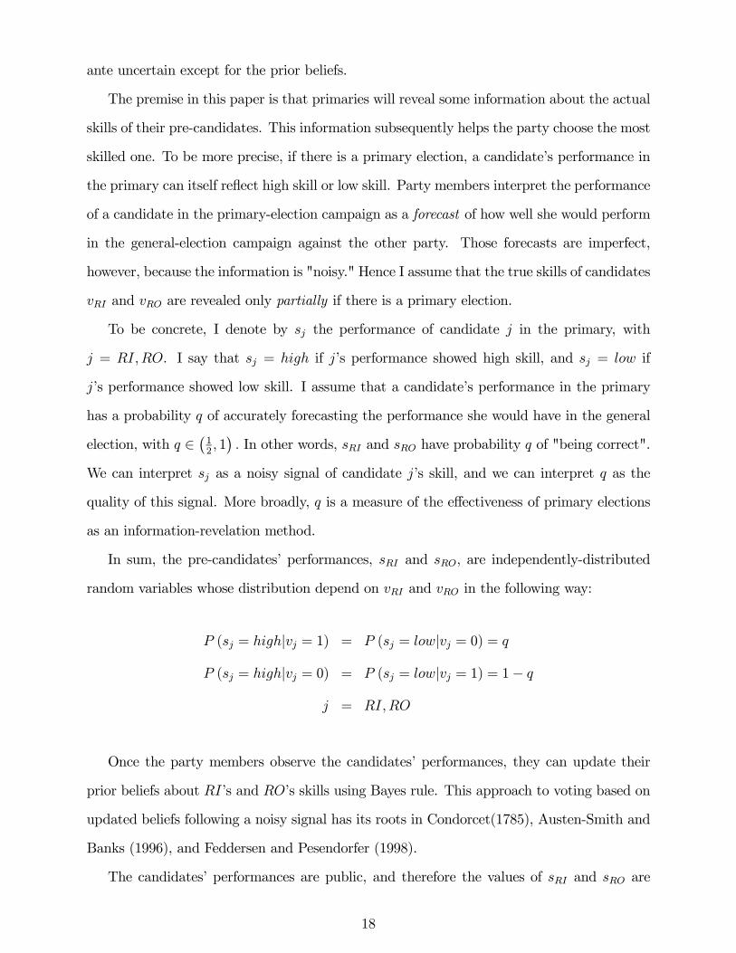
ante uncertain except for the prior beliefs.

The premise in this paper is that primaries will reveal some information about the actual

skills of their pre-candidates. This information subsequently helps the party choose the most

skilled one. To be more precise, if there is a primary election, a candidate’s performance in

the primary can itself reflect high skill or low skill. Party members interpret the performance

of a candidate in the primary-election campaign as a forecast of how well she would perform

in the general-election campaign against the other party. Those forecasts are imperfect,

however, because the information is "noisy." Hence I assume that the true skills of candidates

vRI and vRO are revealed only partially if there is a primary election.

To be concrete, I denote by sj the performance of candidate j in the primary, with

j = RI,RO. I say that sj = high if j’s performance showed high skill, and sj = low if

j’s performance showed low skill. I assume that a candidate’s performance in the primary

has a probability q of accurately forecasting the performance she would have in the general

election, with q ∈ ¡12, 1¢. In other words, sRI and sRO have probability q of "being correct".

We can interpret sj as a noisy signal of candidate j’s skill, and we can interpret q as the

quality of this signal. More broadly, q is a measure of the effectiveness of primary elections

as an information-revelation method.

In sum, the pre-candidates’ performances, sRI and sRO, are independently-distributed

random variables whose distribution depend on vRI and vRO in the following way:

P (sj = high|vj = 1) = P (sj = low|vj = 0) = q

P (sj = high|vj = 0) = P (sj = low|vj = 1) = 1− q

j = RI,RO

Once the party members observe the candidates’ performances, they can update their

prior beliefs about RI’s and RO’s skills using Bayes rule. This approach to voting based on

updated beliefs following a noisy signal has its roots in Condorcet(1785), Austen-Smith and

Banks (1996), and Feddersen and Pesendorfer (1998).

The candidates’ performances are public, and therefore the values of sRI and sRO are

18

common knowledge. In particular, all the RAF members observe the same sRI and sRO, and

hence they update their beliefs based on the same information. Given its interest in winning

the general election, the RAF will vote for the candidate who is believed to have the highest

skill. When a party member is indifferent between RI and RO, I assume she will vote for the

one whose prior probability of being high-skilled was largest. If both have the same prior,

she will randomize equally.

5.2 Primary voters update their beliefs

These elements allow studying the behavior of primary voters. When sRI 6= sRO, I say thata member of party R’s rank and file will "vote according to the signals" if her strategy is to

vote for the pre-candidate whose signal was highest, meaning, whose performance was best

in the primary campaign. On the other hand, if her strategy does not depend on the signals

sent during the primary, meaning that performance in the primary is irrelevant, I say that a

member of party R will "ignore the signals".

These concepts can be used to describe the RAF’s behavior during a primary. As it turns

out, their behavior will depend crucially on their prior belief about the insider candidate’s

valence, πRI . In all the results below, the symbols π and π refer to two constants whose

values are π ≡ (1−q)21−2q+2q2 and π ≡ q2

1−2q+2q2 .

Lemma 1 In a primary election, for each value of πRI, the rank-and-file members of party

R will

• if πRI ∈ (0,π], ignore the signals and always vote for RO

• if πRI ∈¡π, 1

2

¢, vote according to the signals if sRI 6= sRO, and vote for RO if sRI = sRO

• if πRI = 12, vote according to the signals if sRI 6= sRO, and randomize between RI and

RO if sRI = sRO

• if πRI ∈¡12,π¢, vote according to the signals if sRI 6= sRO, and vote for RI if sRI = sRO

• if πRI ∈ [π, 1), ignore the signals and always vote for RI

19

There are several noteworthy features of this result, the first one being how influential

the prior beliefs are: given that each member of R is assumed to be rational and to use

all information available to make her decision, she will combine the prior beliefs about the

candidates with the new information coming from their performance. However, the prior

beliefs might be so compelling that even a Bayesian party member will choose to disregard

the candidates’ performances. In particular, for high enough values of πRI the RAF will

always vote for RI even if it receives strong indications of the insider’s low skill compared

with the outsider’s high skill. Primary voters will simply not trust that such performances

will carry through to the general election. Hence the insider candidate RI is immune against

an open contest with the outsider RO; he will be nominated regardless of their performances.

This result is significant as it opens the possibility that any information revealed during

the primary election will be useless: primary voters might vote according to preexisting

information while completely ignoring the new information.

On the other hand, the results for intermediate values of πRI go in the expected direction:

primary voters will take the signals into account, and will vote for the candidate whose

performance in the primary campaigns was best. Hence the insider candidate I will indeed

be vulnerable to being beaten by the outsider O in an open contest.

Our next task is to quantify the benefit of holding a primary instead of a leadership

selection. As I derive below, the bonus of using a primary election is to increase the expected

skill of the party’s nominee. Hence the value I am looking to find is the difference between

E (vR|primary) and E (vR|elite) .5 It is easy to see that such difference is given by

E (vR|primary)−E (vR|elite) = V · S

with S ≡ P (vR = V |primary)− P (vR = V |elite)

The important value is S, which represents the extra probability of having a high-skilled

candidate that a primary brings above an elite selection. I call it the skill bonus of a primary.

Studying S, how large it is and how it changes, is the main task now. Rather than giving

5We should keep in mind that, even though the actual value of vR is discreet, the expected value E (vR)is continuous.

20

the exact value of S, which comes in the appendix, I will focus on the key properties that

will buttress the rest of the paper. I start by rephrasing the previous considerations in terms

of πR, which is the variable that party R is seeking to maximize.

Theorem 2 The probability that R’s nominee will be high-skilled, πR, given R’s nomination

process, mR, is given by

πR ≡ P (vR = V |mR) =

⎧⎪⎨⎪⎩ πRI if mR = elite

πRI + S if mR = primary

where S is called the primary skill bonus and is given by S ≡ P (vR = V |primary) −P (vR = V |elite)

This demonstrates how the information revealed in primary campaigns is translated into

a better nominee in terms of valence. Holding an internal contest will increase the probability

of nominating a high-skilled candidate in the amount S. Is that a small or a large benefit? I

answer that question in the next subsection.

5.3 What makes primaries more appealing?

I begin by establishing whether primaries have a benefit to party leaders.6

Lemma 2 The primary skill bonus S is strictly positive for πRI ∈ (0,π) and zero for πRI ∈[π, 1).

Primaries therefore do bring a benefit for small enough priors about the insider’s skill.

When the insider candidate is weak, meaning that πRI is below a certain threshold, forcing

her to compete with an outsider candidate increases the excepted skill of the nominee by

a strictly positive amount. The reason is that for πRI ∈ (0,π) party members will take aserious look at the outsider candidate’s performance in the primary to decide whether she

6As mentioned before, the symbols π and π refer to two constants whose values are π ≡ (1−q)21−2q+2q2 and

π ≡ q2

1−2q+2q2 .

21

is more convincing than the party insider. This result was expected as it conforms with

previous findings in Serra (2011).

The surprising result comes from high priors about the insider’s skill: in such case a

primary election might not bring any benefit whatsoever. When the insider candidate is

strong, meaning that πRI is above a certain threshold, forcing her to compete with an

outsider candidate does not increase the expected skill of the nominee at all. The reason is

that for πRI ∈ [π, 1) party members find the insider candidate so compelling that they willvote for her regardless of the outsider candidate’s performance in the primary. This result

is new with respect to the papers about primaries that I am aware of.

It is now turn to study how S changes with a change in its two main determinants: the

prior about the insider candidate’s skill, πRI , and the accuracy of the candidates’ perfor-

mances q. Do they make primaries more or less attractive? I first describe the comparative

statics with respect to πRI .

Lemma 3 The primary skill bonus S is strictly decreasing with πRI for πRI ∈ (0,π) , andconstant (equal to zero) to any increase in πRI for πRI ∈ [π, 1).

Several insights about S can come from the lemma above, most notably that it decreases

with πRI . This makes intuitive sense, because the benefit of primaries is to improve upon the

skill of the candidate that would be nominated through an elite selection, namely the insider

candidate. As the skill of the insider candidate is expected to be higher, it becomes less likely

that a primary will improve upon it. In fact, as mentioned before, this electoral advantage

reaches zero once the insider candidate’s appeal to voters exceeds a certain threshold labeled

π.

The message is that the electoral advantage brought by primaries is larger the less ap-

pealing the insider candidate is to begin with. This is clearly seen in the graph below, which

depicts the value of S as a function πRI .

22

Figure 3: The primary skill bonus S as a function of

the insider’s probability of being high-skilled πRI

I can turn now to studying how S changes with q. Remember that we can interpret q

as the quality of primary elections as an information-revelation method. To be exact, an

increase in q improves the accuracy of the performances sRI and sRO as forecasts of future

performances in the general election. This improvement could occur because the primary

campaigns became longer, or because the media paid more attention to them, or because they

included more challenges like debates on television and so on. In essence, a larger q implies

that the primary performance is a better forecast of the candidate’s campaigning ability

in the general election. Intuition would suggest that any improvement in the primaries’

technology would make those primaries more attractive. Surprisingly, as the following result

shows, this intuition is only correct under certain circumstances.

Lemma 4 The effect on the primary skill bonus S of a marginal increase in q is strictly

positive for πRI ∈ [π,π], but is null for (0,π) and (π, 1) .

The result goes in the expected direction for moderate priors about the insider candidate’s

skill. For intermediate values of the prior πRI , marginal increases in q will indeed increase

S. The reason is that primary voters are unsure about the relative merits of the insider

candidate compared to the unknown outsider that will join the race. They will pay close

attention to the primary campaigns to nominate the candidate with a better performance.

23

A higher quality of the information revealed will increase the probability of making the right

nomination choice. Such an increasing effect is depicted in the figure below.

However, for other priors, the quality of a primary elections will bear no impact on its

benefit. When the insider candidate is expected to be overwhelmingly competent in the

general election, she will be nominated even if her performance in the primary is appalling.

Primary voters will trust that her performance in the primary was due to bad luck. On the

other hand, when the insider candidate is expected to be overwhelmingly unqualified, she

will lose to the outsider candidate even if her performance was better. Primary voters will

believe her performance was just a fluke that does not justify giving her a chance in the

general election. In sum, for extremely high or extremely low values of πRI , primary voters

quickly make up their minds, either to nominate RI for sure or to nominate RO for sure,

regardless of any campaign events that may occur. Improving the quality of primaries by

marginally increasing q will have no effect on this decision.

Figure 4: The effect of increasing the quality of signals q

on the primary skill bonus S

In sum, primaries have two potential benefits: (1) allowing primary voters to replace the

insider candidate with an outsider candidate whose prospect are believed to be superior; and

(2) using new information revealed during the primary campaigns to discriminate between

24

both candidates. As it turns out, whether those benefits actually occur depends crucially

on the prior beliefs about the campaigning skill of the insider candidate. This finding is

qualitatively summarized in the following table.

Table 3: The two potential benefits

of a primary election as a function of πRI

Benefit of primaries

Expectation that RI

is high-skilled, πRI

Replacing RI

with RO

Using the information

revealed during

the primary

Skill bonus

of a primary

S

Low Yes, for sure No, information ignored High

Intermediate Yes, probably Yes, taken into account Low

High No, never No, information ignored Zero

To summarize this section, the benefit, when there is one, of primary elections is a larger

probability of nominating a candidate with a high campaigning skill. I called that extra

probability the primary skill bonus. Primaries might carry a cost however, in terms of the

policy that candidates are induced to adopt. That cost is described in detail in the following

section. As a consequence, the party leadership needs to carry out a cost-benefit analysis

when choosing whether to hold a primary election or not.

6 The cost of primary elections

As we just saw, the benefit to party leaders of adopting a competitive primary election is

to increase the expected skill of their nominee. However, primaries might carry a cost in

terms of the policy that candidates are induced to adopt. To be precise, a primary election

has two differences with respect to an elite endorsement: first, the probability that R’s

nominee is high-skilled increases from πRI to πRI + S. And second, it would be RM and

not RE that R’s candidate would have made policy commitments to; and thus it would be

25

the RAF’s preferences rather than the leadership’s preferences which would determine R’s

policy platform.

By glancing at the table below, we can readily see the trade-off that R’s leadership faces

in choosing a primary election over an elite endorsement. As a benefit, using a primary

increases the probability of nominating a high-skilled candidate (due to the primary skill

bonus S). As a cost, the payoff from having the highest skilled candidate decreases (due to

the internal divergence XRM −XRE). Put differently, a primary makes losing less likely butmakes winning less attractive.

Table 4: The trade-off faced by

party R’s elite

Probability that Utility of RE if

R wins the election R wins the election

Elite selection πRI 0

Primary election πRI + S − |XRE −XRM |

The goal now is to find expressions for the expected utility of R’s leadership by choosing

either a primary election or an elite selection. I call EURE (mR) the expected utility of R’s

leadership from adopting mR as its CSM. It can be derived from Theorem 1, which gives the

outcomes of the election depending on the the value∆v ≡ vR−vL. If L’s candidate has a skilladvantage, she will announce the platformXL and she will win the election. If R’s candidate

has a skill advantage, she will announce the platform XRE if she was nominated by an elite

appointment or she will announce XRM if she was nominated by a primary election; and

either way she will win the election. If L’s candidate and R’s candidate have the same skill,

they will both announce the platform 0 and they will tie in the election. These considerations

lead to the following expressions for EURE (mR) .

26

Lemma 5 The expected utility of R’s leadership for each value of mR is

EURE (mR = elite) = − (XRE −XL)πL (1− πRI)

− (XRE − 0) [πLπRI + (1− πRI)]

− (XRE −XRE) (1− πL)πRI

EURE (mR = primary) = − (XRE −XL)πL (1− (πRI + S))

− (XRE − 0) [πL (πRI + S) + (1− πL) (1− (πRI + S))]

− |XRE −XRM | (1− πL) (πRI + S)

Armed with these results, the leadership in party R can measure the consequences of

choosing one CSM over the other.

7 The optimal selection of a CSM

The leadership in party R will choose the optimal rule mR by comparing EURE (mR = elite)

and EURE (mR = primary). It will choose the CSM that yields the highest expected utility,

and if it is indifferent, I assume that it will choose an elite selection. A primary will be

adopted if and only if EURE (mR = elite) < EURE (mR = primary) . That condition leads

to the following result, recalling that dR ≡ |XRM −XRE|.

Theorem 3 The leadership of party R will adopt a primary election if and only if

dR < T

with T ≡ S[XRE(1−πL)−XLπL](1−πL)(πRI+S) .

The intuition behind this result is that R’s leadership will delegate the nomination if

and only if the RAF’s ideology is close enough to its own. In other words, internal party

democratization will only ensue from enough elite-mass congruence. How close do primary

27

voters need to be to the party elite? It depends on a certain threshold, T , introduced in

the theorem. If the preferences of the elite and the mass of party R are so incongruent

that T ≤ dR then the leadership will not adopt a primary election. This could happen fortwo reasons. On one hand, the RAF could be so far on the right of the leadership that

XRE + T ≤ XRM . In that case the leadership will not adopt a primary election because theprimary voters are too extremist. On the other hand, the RAF could be so far on the left of

the leadership that XRM ≤ XRE − T. In that case the leadership will not adopt a primaryelection because the primary voters are too centrist.

As it turns out, the first reason (that primary voters might be too extreme) is frequently

found in some way or another in scholarly comments about primary elections. Yet the

second reason (that primary voters might be too moderate) is equally intuitive but is seldom

mentioned in the existing literature. The same intuition can be obtained from the figure

below. For low values of XRM (which I label "moderate primary voters") the party will

endorse an insider candidate. For intermediate values of XRM (which I label "partisan

primary voters") the party will hold a competitive primary election. For high values of

XRM (which I label "extremist primary voters") the party will endorse an insider candidate.

Consequently, the CSM has a non-monotonic relationship with the ideal point of the median

primary voter.

28

Figure 5: The candidate-selection method as a function

of the ideal point of the median primary voter, XRM .

From the results above it is clear that the threshold T determines how likely primary

elections are. The interval (XRE − T,XRE + T ) corresponds to the values that XRM should

take for the nomination to be delegated to party members. Such interval can therefore be

interpreted as the likelihood that R will adopt a primary. For a larger T it is more "likely"

that the internal divergence between R’s establishment and RAF will be lead to a primary.

Then a way of phrasing the previous theorem is that the likelihood of opening the CSM

decreases with the internal divergence between the party’s leadership and the primary voters.

7.1 Comparative statics

We would like to gain insight on what makes the adoption of primary elections more likely.

According to the previous theorem, the likelihood of adopting a primary is given by T .

Hence, I study how T changes with the parameters in the model. As it turns out, the results

will crucially depend on the value of πRI , To be specific, I need to divide two cases. The

first case is πRI ∈ (0,π) corresponding to low and intermediate priors, and the second case isπRI ∈ [π, 1) corresponding to high priors. Recall that π and π refer to two constants whose

values are π ≡ (1−q)21−2q+2q2 and π ≡ q2

1−2q+2q2 .

29

I start with low and intermediate prior beliefs about the skill of the insider candidate,

which corresponds to the situation where primaries are most attractive.

Theorem 4 Suppose the initial expectation that RI is high-skilled, πRI , is such that πRI ∈(0,π) . Then the threshold T, which determines the likelihood of primaries, is:

1. Strictly positive

2. Strictly increasing with S

3. Strictly decreasing with πRI

4. Strictly increasing with q if πRI ∈ [π,π) , and insensitive to q otherwise

5. Strictly increasing with πL

6. Strictly decreasing with XL

7. Strictly increasing with XRE

The first two results of this theorem corroborate the benefit of primaries. First, I find

that T > 0. Hence there will always exist a certain distance with the RAF that party leaders

can tolerate for delegating it the nomination decision. Second, this threshold increases with

the primary skill bonus. The larger the primary skill bonus S, the more likely it is that the

elite will forgo appointing the insider in a smoke-filled room.

The third and fourth results decompose the effect of S in its two components, πRI and

q. The effect of the expected competence of the insider candidate is intuitive: the more

competent the insider candidate is, the less likely that a primary will identify a better

candidate, and hence the less attractive primaries are. This effect can be observed in the

figure below which depicts how the likelihood of adopting a primary decreases with the prior

belief about the insider. The comes from Lemma 3 which established the negative effect of

πRI on S, and hence on T.

30

Figure 6: The likelihood of adopting a primary as a function of

the insider’s probability of being high-skilled πRI (all things equal)

The effect of q is also intuitive though more complex. As I mentioned, an increase in

q can be interpreted as an improvement in the information-revelation feature of primaries.

For intermediate values of πRI , an increase in q will increase S as we know from Lemma

3, which in turn will increase T. In other words, a primary election is more attractive for

party leaders when its ability to reveal information is larger. This effect can be observed in

the figure below which depicts how the likelihood of adopting a primary increases when the

quality of primaries increase.

This result contradicts a certain view of primaries in the literature. It is sometimes

advised that primary elections should be short and smooth to avoid candidates draining their

energy and resources (see for example Ezra (2001)). The theorem above provides a different

perspective. A party can actually benefit from having long and challenging primaries, as this

would increase the amount of information revealed about pre-candidates (namely q). This

result is new in the literature about primaries, as it could only be obtained by making the

realistic assumption that primaries can only reveal information partially rather than fully.

The last part of the result is more surprising. For low values of πRI , an increase in q will

not have any effect on T. The reason is that candidates’ performances in the primary would

31

actually being ignored. Primary voters have already made up their minds in favor of an

outsider candidates irrespective of her eventual performance in the primary. So increasing or

decreasing the amount of information will not alter the nomination decision and consequently

will not make primaries more or less attractive.

Figure 7: The effect of increasing the quality of signals q (all things equal)

on the likelihood to adopt a primary

The fourth, fifth and sixth results broadly indicate that disadvantaged parties are more

likely to adopt primaries than advantaged parties. They were all previously found in Serra

(2011) so I do not elaborate on them here. Rather I focus on the importance of πRI which

is a new contribution.

In particular, the following result departs from previous research as it provides conditions

for an insider candidate to avoid a primary challenge. As it turns out, an insider might have

a good enough reputation that party leaders will inevitably nominate her by not opening the

competition to outsiders under any circumstance.

Theorem 5 Suppose the initial expectation that RI is high-skilled, πRI , is such that πRI ∈[π, 1) . Then the threshold T, which determines the likelihood of primaries, is zero and pri-

maries will never be adopted under any value of the other parameters.

In other words, the insider’s reputation could be so good that leaders will inexorably

32

appoint her. This type or reputation could be enjoyed, for example, by an incumbent who

has already won a previous election. Strikingly, a primary election will be eschewed even

if primaries reveal a maximum amount of information; even is there is perfect congruence

between the elite and the membership of the party; and even if party R has important

weaknesses with respect to L. There exists a threshold above which πRI will prevent the use

of primary elections for all values of q, XRM , XRE, XL and πL.

Hence this result provides an explanation for the empirical observation that many incum-

bents get re-nominated in their parties without a primary challenge. The reason is that for

sufficiently high expectations about the insider candidate’s skill, primaries do not bring any

advantage at all: both the RAF and the elite are sure to nominate the same candidate. This

comes from Lemma 2. Given that primaries do not bring a benefit, any amount of elite-mass

incongruence is enough to deter party democratization. S is equal to zero and hence T is

equal to zero, which means that any value of dR is intolerable for party leaders.

8 Conclusions and discussion

When can an incumbent or any well-known insider feel safe against a challenge for the

nomination of a future election? When can he or she be confident that party leaders will

directly appoint her rather than holding a competitive primary election? Primary elections

are a frequent method used by political parties around the world to select their candidates

—and increasingly so. The premise in this paper is that primary elections can serve as

a mechanism to reveal information about the candidates’ personal appeal to voters. In

particular, by forcing candidates to run a primary campaign before the general election

campaign, the candidates reveal their campaigning skills and the primary voters can select

them accordingly.

An implication of those two features is that a primary election will increase the expected

valence of the party’s nominee. Such benefit has been modeled previously, for example in

Adams and Merrill (2008), Serra (2011) and Snyder and Ting (2011), and indeed the findings

in this paper corroborates some of the findings in that previous literature (for example that

33

primaries are most beneficial to the weakest parties as found by Adams and Merrill (2008)

and Serra (2011)).

However those models assume that primaries reveal information fully, meaning that can-

didates’ performance in the primary are a perfect forecast of their performance in the general

election. In contrast, this paper assumes that primaries only reveal information partially,

meaning that candidate’s performance in the primary are a noisy and imperfect forecast of

their performance in the general election.

Making this realistic assumption led to new insights. The prior reputation of the party

insider (the parameter πRI) turns out to play a crucial role in deterring the use of primaries.

Primaries are less appealing to party leaders the better the insider candidate is believed to

be. In fact, if the party insider has a good enough reputation for winning votes, for example

by virtue of being an incumbent who won a previous election, then a primary election will

be eschewed altogether. The paper thus provides an explanation for the empirical fact that

many incumbents get re-nominated by their parties without a primary challenge.

This new setup also allowed studying the behavior of primary voters more precisely. As

expected, primary voters may use the information provided by primary campaigns to select

the pre-candidate with a most impressive performance. However, as it turns out they will

only do so for moderate expectation about the ability of the insider candidate. If, on the

other hand, the insider is believed to be extremely competent or extremely incompetent,

primary voters will actually ignore the contenders’ performance in the primary campaigns

and vote exclusively according to their preexisting priors.

I finish with a prescriptive note. If we believe that democratization should occur in

any representative institution, we should care about when and why political parties become

internally democratic. A question for reformers, then, is how to make competitive primary

elections more prevalent. This paper provides several suggestions, but the most direct one

is to improve the revelation of information during the primary cycle (the parameter q).

Political parties and the general public can benefit from improving the design of primaries

to test the precandidates’ campaigning skills thoroughly enough. For example, parties could

include more debates, make campaigns longer, and allow tough critiques among contenders.

34

In other words, the more challenging primaries are, the more information they will reveal

about the precandidates. A recent example is the competition between Hillary Clinton and

Barack Obama during the Democratic primary election. Several Democratic supporters

complained that the competition between Clinton and Obama was too long and too severe.

Those Democrats worried about the possible costs to their party’s prospects in the general

election. I do not deny that such costs existed: the potential drawbacks of a competitive

primary election include division and resentment among the party base, among other possible

costs. But this paper points to a benefit that was seldommentioned during the 2008 primary.

Observers claimed that too much information was being revealed about Clinton and Obama—

information which could later be misused by the Republicans. My premise, however, is that

such information would have been revealed anyway in the course of the general-election

campaign. As a consequence, it was beneficial for the Democratic sympathizers to acquire

that information beforehand to help them select their nominee wisely. According to this

paper, the length and intensity of the primary campaign are not necessarily a curse for the

party, but could actually be a blessing.

A Appendix with the proofs

A.1 Proof of Theorem 1

Table 1 here is a particular case of Table 1 in Theorem 1 of Serra (2011).

A.2 Proof of Lemma 1

Proof of Lemma 1. If there is a primary election, Party R’s RAF will vote for the

candidate that it believes to have highest probability of being high-skilled. The beliefs it

holds about each candidate’s skill depend on two pieces of information: its prior beliefs, and

the information acquired throughout the primary campaign. Given that the RAF members

are rational, they will update their prior beliefs based on the performances sRI and sRO to

form a couple of posterior beliefs about the probabilities that RI and RO are high-skilled.

35

If the RAF uses Bayes Rule to update its prior beliefs after receiving a given estimate, its

posterior beliefs will be given by

P (vRI = 1|sRI = low) =(1− q) πRI

(1− q)πRI + q (1− πRI)

P (vRI = 1|sRI = high) =qπRI

qπRI + (1− q) (1− πRI)

P (vRO = 1|sRO = low) = 1− q

P (vRO = 1|sRO = high) = q

There are four couple of performances (sRI , sRO) that the RAF could observe, which are

(0, 0) , (1, 1) , (0, 1) and (1, 0) , I study each of them in turn, along with the decision that the

RAF makes upon receiving those couples of estimates.

• If the RAF observes sRI = low and sRO = low :

The RAF will vote forRI if P (vRO = 1|sRO = low) < P (vRI = 1|sRI = low) which isequivalent (after some algebra) to 1

2< πRI . Then, given my indifference assumption, the

RAF will vote for RO if πRI < 12, will vote for RI if 1

2< πRI , and will randomize equally if

πRI =12.

• If the RAF observes sRI = high and sRO = high :

The RAF will vote forRI if P (vRO = 1|sRO = high) < P (vRI = 1|sRI = high) which isequivalent (after some algebra) to 1

2< πRI . Then, given my indifference assumption, the

RAF will vote for RO if πRI < 12, will vote for RI if 1

2< πRI , and will randomize equally if

πRI =12.

• If the RAF observes sRI = low and sRO = high :

The RAF will vote forRI (in other words, disregard the candidates’ performance) if

P (vRO = 1|sRO = high) < P (vRI = 1|sRI = low) which is equivalent (after some algebra,and noting that 1−2q+2q2 > 0) to q2

1−2q+2q2 < πRI . Then, given my indifference assumption

(and noting that 12< q2

1−2q+2q2 ), the RAF will vote for RI if and only π ≤ πRI , with

π ≡ q2

1−2q+2q2 .

36

• If the RAF observes sRI = high and sRO = low :

The RAF will vote forRO (in other words, disregard the candidates’ performance) if

P (vRO = 1|sRO = low) < P (vRI = 1|sRI = high) which is equivalent (after some algebra,and noting that 1−2q+2q2 > 0) to πRI < (1−q)2

1−2q+2q2 . Then, given my indifference assumption

(and noting that (1−q)21−2q+2q2 <

12), the RAF will vote for RO if and only πRI ≤ π, with

π ≡ (1−q)21−2q+2q2 .

The following table summarizes these results:

sRI = low sRI = high sRI = low sRI = high

sRO = low sRO = high sRO = high sRO = low

if πRI ∈ (0,π] Vote for RO Vote for RO Vote for RO Vote for RO

if πRI ∈¡π, 1

2

¢Vote for RO Vote for RO Vote for RO Vote for RI

if πRI = 12

Randomize Randomize Vote for RO Vote for RI

if πRI ∈¡12,π¢Vote for RI Vote for RI Vote for RO Vote for RI

if πRI ∈ [π, 1) Vote for RI Vote for RI Vote for RI Vote for RIWhich is what the lemma claims.

A.3 Proof of Theorem 2

Proof of Theorem 2. This conclusion comes directly from two observations: (1) With an

elite selection, the party will directly appoint RI, and thus P (vR = V |mR = elite) = πRI .

And (2) with a primary election the probability of nominating a high-skilled candidate will

increase by S by definition, such that P (vR = V |mR = primary) = πRI + S.

A.4 Proof of Lemma 2

Proof of Lemma 2. I start by calculating the exact value of S. All its properties are

derived from this value. We can use the RAF’s behavior described in the previous lemma.

For that, I first need to calculate P (vR = V |primary) . We can do so by noting that

37

P (vR = V |primary) =XvRI ,vRO

XsRI ,sRO

P (vR = V |primary, sRI , sRO; vRI , vRO) · P (sRI , sRO|vRI , vRO) · P (vRI , vRO)

which uses the definition of conditional probability twice.

Each summand in that expression is straightforward to calculate. P (vRI , vRO) depends

only on the prior probabilities that vRI and vRO are high-skilled, which are πRI for the insider

and 12for the outsider. P (sRI , sRO|vRI , vRO) depends only on the accuracy of the signals,

which is q. And P (vR = V |primary; sRI , sRO; vRI , vRO) depends on how the RAF will votegiven the candidates’ performances, which I just computed in the table above. Multiplying

and adding those probabilities is easy but too long to develop here (the detailed calculations

are reported in previous versions of this paper). With the appropriate algebra we find that

P (vR = V |primary) =

⎧⎪⎪⎪⎪⎪⎪⎪⎪⎪⎪⎨⎪⎪⎪⎪⎪⎪⎪⎪⎪⎪⎩

12if πRI ∈ (0,π]

πRIq2 + q − 1

2q2 − πRIq +

12πRI if πRI ∈

¡π, 1

2

¢12q + 1

4if πRI = 1

2

πRIq − πRIq2 + 1

2q2 + 1

2πRI if πRI ∈

¡12,π¢

πRI if πRI ∈ [π, 1)

I can now calculate the value of interest, S. The values above are used to calculate S ≡P (vR = V |primary)− P (vR = V |leadership) , remembering that P (vR = V |leadership) =πRI . With some algebra and noting the continuity of S at πRI = π, πRI =

12and πRI = π,

we find that

S =

⎧⎪⎪⎪⎪⎪⎪⎪⎨⎪⎪⎪⎪⎪⎪⎪⎩

12− πRI for πRI ∈ (0,π]

πRIq2 − πRIq − 1

2q2 − 1

2πRI + q for πRI ∈

£π, 1

2

¤−πRIq2 + πRIq +

12q2 − 1

2πRI for πRI ∈

£12,π¤

0 for πRI ∈ [π, 1)

which are the values we were looking for.

38

Now we need to analyze the sign of S. If πRI ∈ (0,π] we have that S = 12− πRI >

0 ⇔ πRI <12, but that is satisfied because πRI ≤ π and I have already noted that π < 1

2.

If πRI ∈£π, 1

2

¤we have that S = πRIq

2 − πRIq − 12q2 − 1

2πRI + q > 0 ⇔ πRI <

2q−q21+2q−2q2

(noting that 1 + 2q − 2q2 > 0) which is satisfied because 12< 2q−q2

1+2q−2q2 . If πRI ∈ [12 ,π) wehave that S = −πRIq2+ πRIq+

12q2− 1

2πRI > 0⇔ πRI <

q2

1−2q+2q2 which is satisfied because

π = q2

1−2q+2q2 . And finally if πRI ∈ [π, 1) we have S = 0. So we have indeed S > 0 for

πRI ∈ (0,π] ∪£π, 1

2

¤ ∪ [12,π) and S = 0 for πRI ∈ [π, 1), as the lemma claims.

A.5 Proof of Lemma 3

Proof of Lemma 3. I calculate the differential of S with respect to πRI and check its sign.

If πRI ∈ (0,π), ∂S∂πRI

= −1 which is strictly negative. If πRI ∈¡π, 1

2

¢, ∂S∂πRI

= q2−q−12which is

strictly negative for q ∈ ¡12, 1¢. If πRI ∈

¡12,π¢, ∂S∂πRI

= −q2+2q−1 which is strictly negativefor q ∈ ¡1

2, 1¢. So S is decreasing with πRI in all those intervals. S is non-differentiable at

πRI = π and πRI =12, but is continuos at both points, and is therefore decreasing just like

their neighboring points. Hence S decreases with πRI when πRI ∈ (0,π) ∪ {π} ∪¡π, 1

2

¢∪©12

ª ∪ ¡12,π¢.

If πRI ∈ [π, 1), S is constant for all values of πRI (and equal to zero), so an increase inπRI will not affect it.

A.6 Proof of Lemma 4

Proof of Lemma 4. I calculate the differential of S with respect to q and check its sign,

remembering that the values of π and π are π = (1−q)21−2q+2q2 and π = q2

1−2q+2q2 . According to the

values of S in Theorem 1, if π ∈ (0,π), ∂S∂q= 0; similarly if π ∈ (π, 1) , ∂S

∂q= 0. So in those

intervals, S is unresponsive to marginal changes in q.

However, if π ∈ ¡π, 12

¢, ∂S

∂q= 2πq − π + 1− q which is strictly positive; if π = 1

2, ∂S

∂q= 1

2

which is strictly positive; if π ∈ ¡12,π¢, ∂S

∂q= −2πq + π + q which is strictly positive. So in

those intervals, S is strictly increasing with marginal increases in q.

To analyze the cases where π = π and π = π, note that ∂∂q

³(1−q)2

1−2q+2q2´< 0, so with a

39

marginal increase in q, π remains in the intervalh

(1−q)21−2q+2q2 ,

12

iwhere I just proved that S is

increasing with q. Similarly note that ∂∂q

³q2

1−2q+2q2´> 0, so with a marginal increase in q, π

remains in the intervalh12, q2

1−2q+2q2iwhere I just proved that S is increasing with q.

To summarize, S is unresponsive to marginal changes in q for π ∈ (0,π) ∪ (π, 1) , and isstrictly increasing with q for π ∈ {π} ∪ ¡π, 1

2

¢ ∪ ©12

ª ∪ ¡12,π¢ ∪ {π} .

A.7 Proof of Lemma 5

See the proof of Lemma 1 in Serra (2011).

A.8 Proof of Theorem 3

See the proof of Theorem 2 in Serra (2011).

A.9 Proof of Theorem 4

Proof of Theorem 4. For points 1, 2, 5, 6 and 7, see the proof of points 1, 2, 6, 7 and 8

of Theorem 4 in Serra (2011), respectively.

To study the effect of q (point 3 in the theorem), we note that it only has an indirect

effect on T through its effect on S. I proved in Lemma 5 that q has a strictly positive effect

on S whenever for πRI ∈ [π,π] . And I have proved (in point 2 of the theorem) that S hasa strictly positive effect on T. Therefore, combining both partial derivatives, I prove that q

has a strictly positive effect on T whenever for πRI ∈ [π,π] .To study the effect of πRI we must note that it has two effects on T : a direct effect, and

an indirect effect through its effect on S. In total, we have that dTdπRI

= ∂T∂πRI

+ ∂T∂S

∂S∂πRI

. It

is easy to calculate that ∂T∂πRI

= −S[XRE(1−πL)−XLπL](1−πL)(πRI+S)2 which is strictly negative. On the other

hand I just calculated that ∂T∂Sis strictly positive, and we know from Lemma 4 that ∂S

∂πRIis

non-positive. We therefore have that dTdπRI

< 0 and T is strictly decreasing with πRI .

40

A.10 Proof of Theorem 5

Proof of Theorem 5. Note from Lemma 2 that S = 0 when πRI ∈ [π, 1). And rememberthat T ≡ S[XRE(1−πL)−XLπL]

(1−πL)(πRI+S) . Hence, when πRI ∈ [π, 1) we have that T = 0 for any value ofthe other parameters.

References

[1] Adams, James and Samuel Merrill, III (2008), ’Candidate and Party Strategies in Two-

Stage Elections Beginning with a Primary,’ American Journal of Political Science, Vol.

52, No. 2, April 2008, pp. 344-359.

[2] Adams, James, Samuel Merrill III, Walter J. Stone and Elizabeth N. Simas (2009),

’When Candidates Value Good Government: A Spatial Model with Applications to

Congressional Elections’, manuscript.

[3] Ashworth, Scott and Ethan Bueno de Mesquita (2007), "Valence Competition and Plat-

form Divergence," Games and Economic Behavior.

[4] Austen-Smith, David and Jeffrey S. Banks (1996), "Information Aggregation, Rational-

ity, and the Condorcet Jury Theorem," The American Political Science Review, Vol.

90, No. 1 (Mar., 1996), 34-45.

[5] Caillaud, Bernard and Jean Tirole (2002), "Parties as Political Intermediaries," Quar-

terly Journal of Economics, Vol. 117, No. 4 (November 2002), pp. 1453-1489.

[6] Callander, Steven. 2008. "Political Motivations." Review of Economics Studies 75: 671-

697.

[7] Calvert, Randall L. (1985), ’Robustness of the Multidimensional Voting Model: Can-

didate Motivations, Uncertainty, and Convergence,’ American Journal of Political Sci-

ence, Vol. 29, p. 69-95.

[8] Carrillo, Juan and Micael Castanheira. 2008. "Information and Strategic Political Po-

larization." Economic Journal 118 July: 845-874.

41

[9] Castanheira, Micael, Benoit S.Y. Crutzen and Nicolas Sahuguet (2008), "Party Orga-

nization and Electoral Competition", mimeo.

[10] Cho, Seok-Ju and Insun Kang (2008), ’Open Primaries and Crossover Voting’, paper

presented at the annual national conference of the Midwest Political Science Association.

[11] Condorcet, Marquis de. [1785](1994). Essai sur l’application de l’analyse a la probabilite

des decisions rendues a la pluralite des voix. Trans. lain McLean and Fiona Hewitt. Paris.

[12] Ezra, Marni (2001), "The Benefits and Burdens of Congressional Primary Elections", in

Congressional Primaries and the Politics of Representation, Peter F. Galderisi, Marni

Ezra and Michael Lyons eds., Rowman & Littlefield Publishers, New York.

[13] Feddersen, Timothy and Wolfgang Pesendorfer (1998), "Convicting the Innocent: The

Inferiority of Unanimous Jury Verdicts under Strategic Voting," The American Political

Science Review, Vol. 92, No. 1 (Mar., 1998), 23-35.

[14] Jackson, Matthew O., Laurent Mathevet and Kyle Mattes (2007), ’Nomination

Processes and Policy Outcomes’, Quarterly Journal of Political Science, Vol. 2, Issue 1,

pp. 67-94.

[15] Kanthak, Kristin and Rebecca B. Morton (2001), ’The Effects of Electoral Rules on

Congressional Primaries’, in Congressional Primaries and the Politics of Representa-

tion, Peter F. Galderisi, Marni Ezra and Michael Lyons eds., Rowman & Littlefield

Publishers, New York.

[16] Kselman, Daniel (2012) "Median-Activists or Median-Voters? A Spatial Model with

Intra-Party Competition. Manuscript, Juan March Institute," manuscript, Juan March

Institute.

[17] Meirowitz, Adam (2005), ’Informational Party Primaries and Strategic Ambiguity’,

Journal of Theoretical Politics, 17(1): 107-136.

[18] Meirowitz, Adam. 2008. "Electoral Contests, Incumbency Advantages, and Campaign

Finance." Journal of Politics 70 (03) July: 681-699.

42

[19] Owen, Guillermo and Bernard Grofman (2006), ’Two-stage electoral competition in

two-party contests: persistent divergence of party positions’, Social Choice and Welfare,

Heidelberg: June 2006. Vol. 26, Issue 3; p. 547.

[20] Roemer, John E. (2001), Political Competition: Theory and Applications, Harvard Uni-

versity Press, Cambridge, MA.

[21] Schofield, Norman. (2007). "The Mean Voter Theorem: Necessary and Sufficient Con-

ditions for Convergent Equilibrium." Review of Economic Studies. 74: 965-980.

[22] Schofield, Norman, Christopher Claassen, Ugur Ozdemir, Evan Schnidman and Alexei

V. Zakharov. 2008. "Party Positioning under Proportional Representation and Plurality

Rule." Center in Political Economy. Washington University. Typescript.

[23] Schofield, Norman and Itai Sened. 2005. "Multiparty Competition in Israel, 1988-96."

British Journal of Political Science 35: 635-663.

[24] Serra, Gilles (2010), "Polarization of What? A Model of Elections with Endogenous

Valence," Journal of Politics, Vol. 72, Issue 2, April 2010, pp. 426-437.

[25] Serra, Gilles (2011), “Why Primaries? The Party’s Trade-off between Policy and Va-

lence,” The Journal of Theoretical Politics, January 2011, 23 (1), pp. 21-51.

[26] Snyder, James M. Jr. and Michael M. Ting (2011), "Electoral Selection with Parties

and Primaries," American Journal of Political Science, Vol. 55, No. 4, October 2011,

pp. 781—795.

[27] Wittman, Donald (1973), ’Parties as Utility Maximizers’, American Political Science

Review, Vol. 67, p. 490-498.

43

Measuring the Latent Quality of Precedent:Scoring Vertices in a Network

John W. Patty∗ Elizabeth Maggie Penn† Keith E. Schnakenberg‡

July 10, 2012

∗Department of Political Science and Center for Political Economy, Washington University in Saint Louis. Email:jpatty@wustl.edu.†Department of Political Science and Center for Political Economy, Washington University in Saint Louis. Email:

penn@wustl.edu.‡Department of Political Science, Washington University in Saint Louis.

1

Politics is rife with situations in which objects or individuals are (either explicitly or implicitly)

assigned scores. Examples of explicit rankings include electoral returns (where a candidate or party’s

score is some function of the votes cast in the election) and legislative roll call votes (where proposals

can be assigned scores according to the support received within the legislature in question). Implicit

rankings characterize an even broader swath of political phenomena, including campaign donations,

lobbying, and international trade.

These scores are of interest for various reasons, of course. In many situations, the participants are

directly interested in the revealed ranking (e.g., electoral returns). In addition, one might be interested in

the scores insofar as they provide some evidence about a true, latent, and unidimensional characteristic

of the scored objects. For simplicity, we refer to this latent characteristic as the quality of the object

in question. Without further context, such a notion is clearly broad. For our purposes, we conceive of

quality as being an amalgamation of any and all factors that cause any object to receive a “point” in

observed contests in the realm in question. For example, the “quality” of a candidate for public office is

a unidimensional factor that summarizes the candidate’s likelihood of receiving the vote of a randomly

drawn voter. So as not to belabor this point, we describe quality simply as the latent characteristic of an

object that increases the likelihood that the object will win a contest.1

In this chapter, we consider a scoring problem that is common in the social sciences – that of estimat-

ing the influence of vertices in a network. Our approach assumes that observed levels of influence relate

to an underlying latent “quality” of the vertices. Though common methods for measuring influence in

networks assume that each vertex has the potential to influence every other vertex, many networks re-

flect temporal, spatial, or other practical constraints that make this assumption implausible. We present

a scoring method that is appropriate for measuring influence in networks where (1) some vertices can-

not form an edge with certain vertices for reasons that are unrelated to their underlying “quality” and

(2) each vertex may be influenced by a different number of other vertices, so that some edges reveal

different amounts of information about the latent “quality” of the influencing vertices.1In terms of “belaboring the point,” one can clearly engage in a discussion about the theoretical plausibility of such a

characteristic describing the objects and contests that one is considering. While this discussion is in general both interestingand important, it is orthogonal to our purposes here. On other words, it is hopefully clear that the methodology we presentand employ in this chapter is useful only to the degree that one believes that the notion the method is designed to detect andestimate—i.e., quality—is theoretically sensible. Accordingly, we set this broader discussion to the side.

2

As an example, we rate the “quality” of Supreme Court decisions, which we define as the likelihood

that the decision will be cited in a future decision. These decisions are readily analyzed by our method

due to their connectedness—the Supreme Court’s explicit usage of previous decisions as precedent for

current and future decisions generates a network structure. The network data enable us to assess some

instances when a given decision “succeeded” (i.e., was cited in a later opinion) or “failed” (i.e., was not

cited in a later opinion). However, because later decisions cannot be cited by earlier opinions, the data

do not allow us to observe whether a given opinion would have been cited by an earlier opinion. Our

network structure is necessarily incomplete.

The method we describe and employ in this chapter is intended to deal explicitly with this problem

of incompleteness. The method, developed and explored in more detail by Schnakenberg and Penn

(2012), is founded on a simple (axiomatic) theoretical model that identifies each opinion’s latent quality

in an (unobserved) world in which every object has the potential to succeed or fail. The theoretical

model identifies the relative quality of the objects under consideration by presuming that the observed

successes are generated in accordance with the independence of irrelevant alternatives (IIA) choice

axiom as described by Luce (1958). In a nutshell, the power of this axiom for our purposes is the ability

to generate scores for alternatives that are not directly compared in the data. Substantively, these scores

locate all opinions on a common scale.

1 Inferring Quality from Network Data

We conceive of our data as a network in this chapter. Accordingly we first lay out some preliminaries and

then discuss how one applies the method to general network data. We represent the observed network

data by a graph denoted by G = (V,E), where V = {1, 2, . . . , n} is a set of n vertices and E is a set

of directed edges, where for any v, w ∈ V , (v, w) ∈ E indicates that that there is an edge from v to w.2

We define a community to be a subset of vertices, C ⊆ V , with a community structure C = (C1, ..., Cn)

being a set of subsets of V , and Ci being the community of vertex i.2In general network settings, we interpret a connection from v to w as implying that w “influences” or “is greater than” v.

What is key for our purposes is that the notion of influence be conceptually tied to the notion of quality, as we have discussedearlier.

3

Underlying our model is an assumption that each vertex j in a community Ci has the potential to

influence vertex i. To define this formally, let E be a set of potential interactions, with E ⊆ E. If

(i, j) ∈ E then we know that i and j interacted with j influencing i, and so it is known that they had the

potential to interact: it is known that j ∈ Ci. On the other hand, of course, (i, k) 6∈ E need not imply

that i could not have been connected to k. Rather, it may be the case that opinion that i could have been

connected to k, but the link was not created for some reason (possibly because k was not of high enough

quality to influence i, possibly because k and i never had an opportunity to interact, or for some other

independent factor(s)). Our community structure is designed to accommodate this fact, and in particular

we assume that k ∈ Ci implies that (i, k) ∈ E. Thus, k being in community Ci implies that k had the

potential to influence i (i.e., i had the opportunity to link to k), regardless of whether k may or may not

have succeeded (i.e., regardless of whether an edge between i and k is observed).

The second assumption of our model is that each vertex can be placed on a common scale represent-

ing the vertex’s quality. We assume that vertices with higher latent qualities are more likely to have had

successful (i.e., influential) interactions with vertices that they had the potential to interact with. Thus,

the higher latent quality of vertex i, the more likely that, for any given vertex j ∈ V , (j, i) ∈ E implies

that (j, i) ∈ E.

Our goal is to estimate each vertex’s “latent quality” score subject to a networkG and an observed or

estimated community structure, C. We conceive of our network and community structure as generating a

collection of “contests” in which some vertices were influential, some had the potential to be influential

but were not, and others had no potential to influence. These contests are represented by the set S =

{s ∈ V : (s, v) ∈ E for some v ∈ V }. Thus, every vertex that was influenced represents the outcome

of a contest.

Let x = (x1, ..., xn) ∈ Rn represent each vertex’s latent quality. Then for each i ∈ S we let the

expected influence of vertex k in contest i (i.e., probability of i connecting to k), which we denote by

E(i, k), equal 0 if (i, k) 6∈ E. Thus, k’s expected influence in contest i is zero because in this opinion

we assume that k 6∈ Ci, and thus k had no potential to influence i (i.e., there is no chance that i will

4

connect to k). Otherwise,

E(i, k) =xk∑

j∈Ci

xj.

In words, the expected share of influence of k in a contest in which k has the potential to influence i

is k’s share of latent influence relative to the total latent influence of the vertices that can potentially

influence i.

Similarly, we can calculate the share of actual influence of k in i, or A(i, k), by looking at the total

set of vertices that actually influenced i in the network described by G. This set is Wi = {w : (i, w) ∈

E} ⊆ Ci, and (without any additional information such as edge weights), k’s share is 1|Wi| if k ∈ Wi

and 0 otherwise. We can now utilize our network and community structure to estimate x subject to an

unbiasedness constraint that is conditional on the community structure. The constraint is that

∑s∈S

E(s, i) =∑s∈S

A(s, i) for all i,

or that each vertex’s total actual score equals their total expected score. Satisfaction of this constraint

implies, given a correct community structure, that no vertex is estimated to be more or less influential

than it actually was. Schnakenberg and Penn (2012) prove that, subject to a minimal connectedness con-

dition, there exists a vector x∗ = (x∗1, ..., x∗n) that solves the above system of equations and that is unique

up to scalar multiplication.3 Viewed substantively, this vector represents the relative qualities/influences

of the different nodes. In particular, as x∗ is uniquely identified up to scalar multiplication, the ratio of

any two nodes’ qualities,

ρij ≡xixj,

is uniquely identified. This ratio ρij represents the hypothetical relative frequency of selection/influence

by node i versus that by node j in a future contest in which both nodes i and j compete (i.e., for any

future node that both i and j have the ability to exert influence on).3For reasons of space, we refer the interested reader to Schnakenberg and Penn (2012) for more details on the method.

5

2 Measuring the Quality of Precedent

The use of judicial precedent by Supreme Court Justices–and, in particular, a focus on citations as an

indication of this usage—has attracted sustained attention from legal and political science scholars for

over 60 years.4 Unsurprisingly, given the breadth of the topic, scholars have adopted various approaches

to the study of precedent, but most have focused on the determinants of citation: in a nutshell, what

factor or factors of an opinion augur revisitation of the opinion in future opinions?

Because our model imputes unobserved relationships between objects, it is particularly well-suited

to analyzing networks in which certain links are impossible to observe. These types of networks could,

for example, arise in situations in which vertices are indexed by time and a later vertex is incapable of

influencing a vertex that preceded it.

We utilize a data set consisting of the collection of citations by United States Supreme Court ma-

jority opinions to Supreme Court majority opinions from 1791 to 2002. Thus, viewed in the theoretical

framework presented above in Section 1, the vertices of our network are Supreme Court majority opin-

ions, and if majority opinion i cites majority opinion j, we include the edge (i, j) ∈ E.

Before moving on, it is important to note what we are explicitly abstracting from in our opera-

tionalization of the judicial citation/precedent network. Most importantly, we omit consideration of all

opinions other than the majority opinion. Both dissenting and concurring opinions are relevant for un-

derstanding both the bargaining processes at work in constructing the majority opinion and inferring the

role and quality of precedent (e.g., Carrubba et al. (2011)).5 In addition, our approach ignores the citing

opinion’s treatment of the cited opinion (e.g., favorable, critical, or distinguishing).6 7 We leave each of

these for future work.4Seminal offerings include Merryman (1954) and Landes and Posner (1976), while more recent, book-length analyses

include Hansford and Spriggs II (2006) and Gerhardt (2008). Other relevant citations are provided where appropriate in ourdiscussion.

5In addition, there are many interesting theoretical and empirical questions regarding how one should conceive of therelationship between opinions and opinions (e.g., Bommarito, Katz and Zelner (2009)) that the data we employ here do notallow us to explore more fully.

6Practically speaking, there are a number of ways that scholars have developed and employed to consider this aspect ofhow Justices cite earlier opinions. For recent examples, see Clark and Lauderdale (2010) and Spriggs II, Hansford and Stenger(2011).

7We are not aware of any recent work that has differentiated citations by the number of times the citation occurs in theciting opinion.

6

Differentiating Cases: Community Structure. As discussed earlier, the method we employ allows

us to compare/score objects that have not been directly compared. Accordingly, it offers an analyst

the freedom to “break up” the data in the sense of estimating (or, perhaps, observing) communities of

objects that are less likely to be directly compared with one another. For the purposes of this chapter,

we take into account only the temporal bias discussed earlier—later opinions cannot be cited by ear-

lier opinions—and presume that each opinion is eligible (i.e., “in competition”) for citation by every

subsequently rendered opinion.8

Thus we construct the community Ci for a given opinion i as follows. Letting Year(i) be the year in

which opinion i was heard, we assume that for any pair of vertices (i.e., majority opinions), i, j,

Year(i) > Year(j)⇔ j ∈ Ci.

In words, an opinion can be influenced by any and only opinions that strictly predate it.

Data. We apply our method to Fowler and Jeon’s Supreme Court majority opinion citation data

(Fowler et al. (2007); Fowler and Jeon (2008)). There are a number of ways one might approach this

data when considering the question of the quality or influence of each opinion. The most straightforward

approach would rank all of the opinions that have been cited at least once (any opinion that is not cited

by any other opinion in the database cannot be ranked). In this approach, every opinion is a contest, and

each opinion that is cited at least once is a contestant.

Practical constraints prohibit us from ranking all of the opinions. Fortunately, our approach implies

that we can examine any subset of the data and recover relative rankings that are (in theory) identical to

the rankings that would be estimated from the entire data set. Accordingly, we restrict our attention to

the 100 most frequently cited opinions between 1946 and 2002. In graph theoretic terms, we examine

the smallest subgraph containing all edges beginning or ending (or both) with an opinion whose in

degree (number of times cited) ranks among the top 100 among the opinions rendered between 19468Note that, for simplicity, we approximate this “later than” relation in the sense that we presume (unrealistically) that, in

any year, the Court cannot cite one opinion that is decided in that year in another opinion that is decided in that same year.Given the number of years that we consider, this approximation affects a very small proportion of the number of potentialcitations we consider.

7

and 2002. This graph contains many more than 100 opinions (3674, to be exact). After these opinions,

and their incident edges, are selected, they are then used for our community detection algorithm, which

we now describe.

Using the years of the opinions to create the communities as described earlier, we then solve for

the influence scores of the opinions (i.e., contestants) as follows. First, we choose the contestants in

turn and, for each majority opinion (i.e., contest) that was subsequent to an opinion and cited at least

one member of the contestant’s community, we count the contestant as having been participant (i.e.,

available for citation) in that majority opinion/contest. If the contestant was cited in (i.e., won) that

contest, the contestant is awarded 1/|W | points, where W is the set of opinions (contestants) cited in

that majority opinion (contest). Otherwise, the contestant is awarded 0 points in that contest. With

this vector of scores for each contestant in each contest, it is then possible to directly apply the method

developed by Schnakenberg and Penn (2012) to generate the latent influence scores of each majority

opinion, x = (x1, . . . , xn).

These latent influence scores represent, in essence, the appeal of each majority opinion as a poten-

tial citation in any subsequent majority opinion. What this appeal represents in substantive terms is not

unambiguous, of course. It might proxy for the degree to which the opinion is easily understood, the

degree to which its conclusions are broadly applicable,9 or perhaps the likelihood that the policy impli-

cations of the opinion support policies that are supported by a majority of justices in a typical opinion.

Obviously, further study is necessary before offering a conclusion on the micro-level foundations of

these scores. Such research will require inclusion of observed and estimated covariates distinguishing

the various opinions and majority opinions.

3 Results

We now present the results of three related analyses. We first present our results for the 100 most-cited

opinions rendered between 1946 and 2002.10 Following that, we present the results for the 100 most-9Note that this is true despite the presumption that an opinion might have been feasible only in a subset of observed and

subsequent majority opinions.10This time period includes all cases in the Fowler and Jeon data for which Spaeth’s rich descriptive data (Spaeth (N.d.))

are also available.

8

cited opinions since 1800.11 Finally, we consider the 204 most-cited opinions since 1800 with an eye

toward comparing the ranking of the 100 most-cited opinions since 1946 with the ranking of those cases

when all opinions that have been cited at least as many times as these 100 are considered. All rankings

of the cases can be found in the Appendix.

3.1 Top 100 Opinions Since 1946

Table 4 presents the opinions with the top 36 estimated latent quality scores for this period. This is

the set of opinions for which the estimated quality score is greater than 1, which is by construction the

average estimated quality score for the 100 cases.

This ranking is interesting in a number of ways. The top two majority opinions score significantly

higher than all of the others.12 The top-scoring opinion, Chevron, is a well-known case in administrative

law with broad implications for the judicial review of bureaucratic decision-making. The second-ranked

opinion, Gregg, clarified the constitutionality of the death penalty in the United States. Of course, the

third highest scoring opinion is the famous Miranda decision in which the Court clarified the procedural

rights of detained individuals.

Space prevents us from a full-throated treatment of the scores, but a few simple correlations are

of interest. Table 1 presents three Pearson correlation coefficients relating the opinions’ scores with,

respectively, the age of the opinion, the number of subsequent opinions citing the opinion, and the

number of subsequent opinions citing the opinion divided by the age of the opinion.

Correlation (Age, Score): – 0.461Correlation (# Cites, Score): 0.496

Correlation (# Cite/Year, Score): 0.787

Table 1: Descriptive Correlations with Scores. Sample: Top 100 Most-Cited Cases Since 1946

The negative correlation between the age of an opinion and its score is broadly in line with previous

work on the depreciation of the precedential value (or, at least, usage) of judicial opinions.13 It is11This time period includes all cases in the Fowler and Jeon data.12Note that the estimated scores for the top 100 opinions sum to 100, so these two opinions account for over 1/8th of the

sum of the estimated scores. In other words, any opinion that cites exactly one of these 100 cases is predicted to cite eitherChevron or Gregg almost 13% of the time.

13See, for example, Black and Spriggs II (2010).

9

important to note, however, that this effect is potentially at odds with the IIA axiom on which the

scoring algorithm is based. We partially return to this question below when we expand the sample of

opinions.

That the correlation between the opinions’ scores and the number of times each opinion has been

cited by a subsequent Supreme Court majority opinion is positive is not surprising: the score of an

opinion is obviously positively responsive to the number of times that an opinion has been cited, ceteris

paribus. Accordingly, the interesting aspect of the correlation is not that it is positive but, rather, that it is

not closer to 1. Indeed, inspection of Table 4 indicates, a fortiori, that the rankings of the opinions with

respect to the number of citations they have received and with respect to their scores are not identical.

Put another way: the scores are measuring something different than the opinions’ citation counts or, as it

is commonly known in network analysis, the degree centralities of the opinions in the citation network.

Finally, the correlation between the score and the average number of times per year the opinion has

been cited since it was handed down is strongly positive. This highlights the fact that the scores control

for the fact that an opinion cannot cite an opinion that is rendered subsequently. Again, though, it is

important to note that the ranking of the opinions generated by our scores differs from that generated

by the number of citations per year. It is useful to consider the origins of this difference. Specifically,

the distinction arises because of the fact that the IIA axiom on which the method is based implies that

an opinion’s“reward” (or score) for being cited by a subsequent opinion is inversely proportional to the

number of other opinions cited by that opinion. At the extreme, for example, a hypothetical opinion that

cited every previous opinion would compress the scores of the opinions in the sense that the scores of

all opinions that initially had lower than average scores would increase as a result of the citation by the

hypothetical opinion, whereas the scores of all of those opinions with above average scores prior to the

hypothetical opinion would decrease.14

14Recall that the scores are identified only up to multiplication by a positive scalar, implying that they inherently relativescores.

10

3.2 Top 100 Opinions Since 1800

We now present our results for the top 100 most-cited opinions rendered between 1800 and 2002. Table 5

presents the opinions with the top 38 estimated latent quality scores for this period. As with the previous

analysis for the period between 1946 and 2002, this is the set of opinions for which the estimated quality

score is greater than 1.

Comparing these scores with those in Table 4, it is perhaps surprising how similar the two sets

of scores are. In particular, the top three majority opinions are identical and have very similar scores

in the two analyses. Things get interesting at the fourth highest-scoring position. First, the majority

opinion ranked fourth-highest in the 1946-2002 analysis reported in Table 4, Cannon v. University

of Chicago, is not among the top 100 most-cited majority opinions since 1819.15 The fourth highest-

scoring opinion among the 100 most-cited majority opinions since 1819 is Miller v. California, in which

the Court affirmed and clarified the power of state and local governments to place limits on obscenity.

This opinion is, of course, among the top 100 most-cited rendered since 1946, yet ranks only 19th in the

scores reported in Table 4. This point highlights a feature of the scores in both tables: after the top 3 or

4, there is a relatively large “plateau” of scores

Beyond visual inspection, it is useful to reconsider the correlations analogous to those reported in

Table 1. These are displayed in Table 2 and closely conform to the conclusions drawn in the discussion

of the correlations reported in Table 1: older opinions tend to have lower scores, and scores are positively

associated with both number of subsequent citations as well as the average annual rate of subsequent

citation.

Correlation (Age, Score): – 0.466Correlation (# Cites, Score): 0.425

Correlation (# Cite/Year, Score): 0.849

Table 2: Descriptive Correlations with Scores. Sample: Top 100 Most-Cited Cases Since 1800

15In that case, the majority opinion affirmed an individual’s right to sue recipients of federal financial support for genderdiscrimination under Title IX, which calls for gender equity in higher education.

11

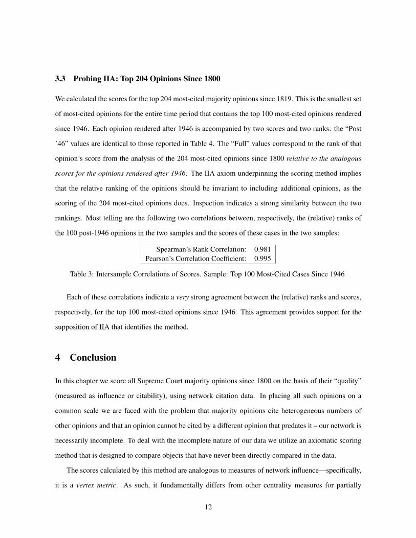
3.3 Probing IIA: Top 204 Opinions Since 1800

We calculated the scores for the top 204 most-cited majority opinions since 1819. This is the smallest set

of most-cited opinions for the entire time period that contains the top 100 most-cited opinions rendered

since 1946. Each opinion rendered after 1946 is accompanied by two scores and two ranks: the “Post

’46” values are identical to those reported in Table 4. The “Full” values correspond to the rank of that

opinion’s score from the analysis of the 204 most-cited opinions since 1800 relative to the analogous

scores for the opinions rendered after 1946. The IIA axiom underpinning the scoring method implies

that the relative ranking of the opinions should be invariant to including additional opinions, as the

scoring of the 204 most-cited opinions does. Inspection indicates a strong similarity between the two

rankings. Most telling are the following two correlations between, respectively, the (relative) ranks of

the 100 post-1946 opinions in the two samples and the scores of these cases in the two samples:

Spearman’s Rank Correlation: 0.981Pearson’s Correlation Coefficient: 0.995

Table 3: Intersample Correlations of Scores. Sample: Top 100 Most-Cited Cases Since 1946

Each of these correlations indicate a very strong agreement between the (relative) ranks and scores,

respectively, for the top 100 most-cited opinions since 1946. This agreement provides support for the

supposition of IIA that identifies the method.

4 Conclusion

In this chapter we score all Supreme Court majority opinions since 1800 on the basis of their “quality”

(measured as influence or citability), using network citation data. In placing all such opinions on a

common scale we are faced with the problem that majority opinions cite heterogeneous numbers of

other opinions and that an opinion cannot be cited by a different opinion that predates it – our network is

necessarily incomplete. To deal with the incomplete nature of our data we utilize an axiomatic scoring

method that is designed to compare objects that have never been directly compared in the data.

The scores calculated by this method are analogous to measures of network influence—specifically,

it is a vertex metric. As such, it fundamentally differs from other centrality measures for partially

12

connected networks such as eigenvector centrality and degree centrality. One difference is that our

measure does not utilize the score of s in computing the contribution of link (s, v) to v’s score (as in

eigenvector centrality); instead our score utilizes the scores of the other w that could have potentially

influenced s, or {w : (s, w) ∈ E}. In generating estimates of the xi using observed network and

community data we impute “influence relationships” between vertices that did not have the potential to

interact. This leads to the following interpretation of our scores: if there were a hypothetical vertex with

a community equal to the set of all possible vertices, then our scores represent the expected influence of

each vertex on that hypothetical vertex.

The analysis presented in this chapter is preliminary, with an obvious shortcoming being the fact

that we assume that the community of a case i, or collection of cases that could potentially influence

i, consists of all of the cases that predate it. In future work we intend to allow community structure to

be determined not only by the year in which a case was considered but also by the topic of the case.

Additionally, we hope to apply our scoring method to other types of incomplete network data as we

believe it provides a useful new measure of node centrality that generalizes the concept of in-degree

centrality.

13

Rank Name Year Score # Cites Cites/Year1 Chevron, U.S.A., Inc. v. NRDC, Inc. 1984 7.52 129 6.82 Gregg v. Georgia 1976 5.14 266 9.93 Miranda v. Arizona 1966 2.72 225 6.14 Cannon v. University of Chicago 1979 2.62 73 35 Younger v. Harris 1971 1.89 129 46 Strickland v. Wash. 1984 1.74 68 3.67 Edelman v. Jordan 1974 1.65 92 3.28 Reynolds v. Sims 1964 1.62 144 3.79 Monell v. Dep’t of Soc. Servs. 1978 1.58 78 3.1

10 Dandridge v. Williams 1970 1.5 132 411 Arlington Heights v. Metro. Hous. Dev. Corp. 1977 1.5 74 2.812 Mathews v. Eldridge 1976 1.49 100 3.713 Buckley v. Valeo 1976 1.49 100 3.714 In re Winship 1970 1.47 131 415 Eddings v. Okla. 1982 1.4 91 4.316 New York Times Co. v. Sullivan 1964 1.38 161 4.117 Baker v. Carr 1962 1.34 149 3.618 Gideon v. Wainwright 1963 1.28 207 5.219 Miller v. California 1973 1.27 131 4.420 Lockett v. Ohio 1978 1.26 104 4.221 Brown v. Board of Education 1954 1.25 155 3.222 Bivens v. Six Unknown Named Agents. . . 1971 1.21 96 323 Monroe v. Pape 1961 1.18 134 3.224 Craig v. Boren 1976 1.17 70 2.625 S.D. Bldg. Trades Council v. Garmon 1959 1.15 89 226 Furman v. Georgia 1972 1.12 118 3.827 Terry v. Ohio 1968 1.1 97 2.828 Warth v. Seldin 1975 1.1 72 2.629 Roe v. Wade 1973 1.08 91 330 Textile Workers Union v. Lincoln Mills 1957 1.08 80 1.731 Wainwright v. Sykes 1977 1.07 71 2.732 Katz v. United States 1967 1.06 127 3.533 Roth v. United States 1957 1.05 155 3.434 Benton v. Maryland 1969 1.04 75 2.235 Stone v. Powell 1976 1.01 80 336 Woodson v. North Carolina 1976 1.01 97 3.6

Table 4: The 36 Highest Scoring Opinions. Sample: Top 100 Most-Cited Cases Since 1946

14

Rank Name Year Score # Cites Cites/Year1 Chevron, U.S.A., Inc. v. NRDC, Inc. 1984 7.21 129 6.82 Gregg v. Georgia 1976 5.82 266 9.93 Miranda v. Arizona 1966 3.28 225 6.14 Miller v. California 1973 2.04 131 4.45 Younger v. Harris 1971 2.03 129 46 Erie R.R. v. Tompkins 1938 1.92 189 2.97 Reynolds v. Sims 1964 1.89 144 3.78 Mathews v. Eldridge 1976 1.84 100 3.79 In re Winship 1970 1.78 131 4

10 Dandridge v. Williams 1970 1.76 132 411 Baker v. Carr 1962 1.73 149 3.612 Buckley v. Valeo 1976 1.58 100 3.713 Monroe v. Pape 1961 1.57 134 3.214 Brown v. Board of Education 1954 1.54 155 3.215 Edelman v. Jordan 1974 1.51 92 3.216 Gideon v. Wainwright 1963 1.5 207 5.217 New York Times Co. v. Sullivan 1964 1.48 161 4.118 Eddings v. Okla. 1982 1.44 91 4.319 Bivens v. Six Unknown Named Agents. . . 1971 1.41 96 320 Chapman v. California 1967 1.39 130 3.621 Lockett v. Ohio 1978 1.38 104 4.222 Furman v. Georgia 1972 1.36 118 3.823 Paris Adult Theatre I v. Slaton 1973 1.33 103 3.424 Morrissey v. Brewer 1972 1.32 94 325 San Diego Bldg. Trades Council v. Garmon 1959 1.29 89 226 Duncan v. Louisiana 1968 1.26 107 3.127 Roth v. United States 1957 1.25 155 3.428 Katz v. United States 1967 1.25 127 3.529 Terry v. Ohio 1968 1.22 97 2.830 United States v. Socony-Vacuum Oil Co. 1940 1.2 113 1.831 Red Lion Broadcasting Co. v. FCC 1969 1.17 87 2.632 Roe v. Wade 1973 1.16 91 333 Goldberg v. Kelly 1970 1.14 97 2.934 Woodson v. North Carolina 1976 1.13 97 3.635 Johnson v. Zerbst 1938 1.07 159 2.436 NAACP v. Alabama ex rel. Patterson 1958 1.05 153 3.437 Ashwander v. Tennessee Valley Authority 1936 1.03 180 2.738 Phelps Dodge Corp. v. NLRB 1941 1.02 88 1.4

Table 5: The 38 Most Influential Cases Among the Top 100 Most-Cited Cases Since 1800

15

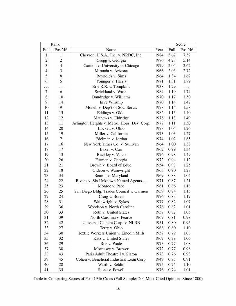
Rank ScoreFull Post’46 Name Year Full Post’46

1 1 Chevron, U.S.A., Inc. v. NRDC, Inc. 1984 5.67 7.522 2 Gregg v. Georgia 1976 4.23 5.143 4 Cannon v. University of Chicago 1979 2.04 2.624 3 Miranda v. Arizona 1966 2.03 2.725 8 Reynolds v. Sims 1964 1.34 1.626 5 Younger v. Harris 1971 1.31 1.89. . . . . . Erie R.R. v. Tompkins 1938 1.29 . . .7 6 Strickland v. Wash. 1984 1.19 1.748 10 Dandridge v. Williams 1970 1.17 1.509 14 In re Winship 1970 1.14 1.47

10 9 Monell v. Dep’t of Soc. Servs. 1978 1.14 1.5811 15 Eddings v. Okla. 1982 1.13 1.4012 12 Mathews v. Eldridge 1976 1.13 1.4913 11 Arlington Heights v. Metro. Hous. Dev. Corp. 1977 1.11 1.5014 20 Lockett v. Ohio 1978 1.04 1.2615 19 Miller v. California 1973 1.03 1.2716 7 Edelman v. Jordan 1974 1.02 1.6517 16 New York Times Co. v. Sullivan 1964 1.00 1.3818 17 Baker v. Carr 1962 0.99 1.3419 13 Buckley v. Valeo 1976 0.98 1.4920 26 Furman v. Georgia 1972 0.94 1.1221 21 Brown v. Board of Educ. 1954 0.93 1.2522 18 Gideon v. Wainwright 1963 0.90 1.2823 34 Benton v. Maryland 1969 0.88 1.0424 22 Bivens v. Six Unknown Named Agents. . . 1971 0.87 1.2125 23 Monroe v. Pape 1961 0.86 1.1826 25 San Diego Bldg. Trades Council v. Garmon 1959 0.84 1.1527 24 Craig v. Boren 1976 0.83 1.1728 31 Wainwright v. Sykes 1977 0.82 1.0729 36 Woodson v. North Carolina 1976 0.82 1.0130 33 Roth v. United States 1957 0.82 1.0531 39 North Carolina v. Pearce 1969 0.81 0.9832 42 Universal Camera Corp. v. NLRB 1951 0.80 0.9533 27 Terry v. Ohio 1968 0.80 1.1034 30 Textile Workers Union v. Lincoln Mills 1957 0.79 1.0835 32 Katz v. United States 1967 0.78 1.0636 29 Roe v. Wade 1973 0.77 1.0837 38 Morrissey v. Brewer 1972 0.77 0.9838 43 Paris Adult Theatre I v. Slaton 1973 0.76 0.9339 45 Cohen v. Beneficial Industrial Loan Corp. 1949 0.75 0.9140 28 Warth v. Seldin 1975 0.75 1.1041 35 Stone v. Powell 1976 0.74 1.01

Table 6: Comparing Scores of Post 1946 Cases (Full Sample: 204 Most-Cited Opinions Since 1800)

16

References

Black, Ryan C. and James F. Spriggs II. 2010. “The Depreciation of US Supreme Court Precedent.”

Working Paper, Washington University in Saint Louis.

Bommarito, II, Michael J., Daniel Katz and Jon Zelner. 2009. Law as a Seamless Web? Comparison

of Various Network Representations of the United States Supreme Court Corpus (1791-2005). In

Proceedings of the 12th International Conference on Artificial Intelligence and Law. ICAIL ’09

pp. 234–235.

Carrubba, Cliff, Barry Friedman, Andrew D. Martin and Georg Vanberg. 2011. “Who Controls the

Content of Supreme Court Opinions?” American Journal of Political Science 56(2):400–412.

Clark, Tom S. and Benjamin Lauderdale. 2010. “Locating Supreme Court Opinions in Doctrine Space.”

American Journal of Political Science 54(4):871–890.

Fowler, James H. and Sangick Jeon. 2008. “The Authority of Supreme Court Precedent.” Social Net-

works 30(1):16–30.

Fowler, James H., Timothy R. Johnson, James F. Spriggs II, Sangick Jeon and Paul J. Wahlbeck. 2007.

“Network Analysis and the Law: Measuring the Legal Importance of Supreme Court Precedents.”

Political Analysis 15(3):324–346.

Gerhardt, Michael J. 2008. The Power of Precedent. New York, NY: Oxford University Press.

Hansford, Thomas G. and James F. Spriggs II. 2006. The Politics of Precedent on the US Supreme

Court. Princeton, NJ: Princeton Univ Pr.

Landes, William M. and Richard A. Posner. 1976. “Legal Precedent: A Theoretical and Empirical

Analysis.” Journal of Law and Economics 19(2):249–307.

Luce, R. Duncan. 1958. Individual Choice Behavior. New York, NY: John Wiley.

Merryman, John Henry. 1954. “The Authority of Authority: What the California Supreme Court Cited

in 1950.” Stanford Law Review 6(4):613–673.

17

Schnakenberg, Keith and Elizabeth Maggie Penn. 2012. “Scoring from Contests.” Working Paper,

Washington University in Saint Louis.

Spaeth, Harold J. N.d. The United States Supreme Court Database. Center for the Empirical Research

in the Law.

Spriggs II, James, Thomas Hansford and Anthony Stenger. 2011. “The Information Dynamics of Verti-

cal Stare Decisis.” Working paper, Washington University in Saint Louis.

18

The Politics of Austerity: Modeling British Attitudes Towards Public Spending Cuts

Harold D. Clarke University of Texas at Dallas and University of Essex

clarke475@msn.com

Marianne C. Stewart University of Texas at Dallas

mcmstewart@gmail.com

David Sanders University of Essex

sanders@essex.ac.uk

Paul Whiteley University of Essex

whiteley@essex.ac.uk

Version: March 19, 2012

1

The Politics of Austerity: Modeling British Attitudes

Towards Public Spending Cuts

Are there no prisons?....And the union workhouses, are they still in operation? Ebenezer Scrooge to Charity Collector, 1851

Beginning in 2008 financial crises and ensuing economic turbulence have prompted

acrimonious national debates in many Western democracies over the need for substantial

budget cuts and debt reductions. Among economic and political elites there is broad

agreement that substantial public sector budget cuts are necessary to address unsustainable

sovereign debt loads and establish long-term fiscal integrity. Many ordinary citizens see

things differently—proposed austerity measures threaten programs that aid the disadvantaged

while challenging longstanding public commitments to education, health and personal

security that constitute the foundation of the modern welfare state. Coming close on the

heels of massive, widely publicized bailouts of major banks, investment firms and

manufacturing companies, the proposed reductions in public sector spending threaten to

overturn the distributional policy consensus in contemporary mature democracies.

As of this writing, several countries—inter alia, Ireland, Italy, Greece, Portugal,

Spain, the United States and the United Kingdom—either have implemented or are seriously

contemplating large-scale budget cuts that will necessitate painful reductions in public

services and benefits. Perhaps the best known case is Greece where the European Union and

the International Monetary Fund have dictated draconian financial policies to remedy the

country's sovereign debt crisis. The result has been widespread, oftentimes violent, public

protests and ongoing political turmoil. In the United Kingdom, proposed public-sector cuts

have prompted civil unrest and charges that the Conservative-led Coalition government

2

accords higher priority to enacting a neo-Thatcherite ideological agenda of small government

and re-privatization than the provision of effective health care and education for its citizens.

This study focuses on the British experience. Confronted with a pernicious

combination of rising public debt and growing unemployment when his coalition government

of Conservatives and Liberal Democrats assumed power in May 2010, Prime Minister David

Cameron and his Chancellor of the Exchequer, George Osborne, proposed to cut an average

of 20 percent from government spending over the next four years (Burns 2010). The plan was

to reduce the budget by £83 billion by eliminating 490,000 government jobs, curtailing

benefits, and chopping a broad range of "unnecessary" programs (BBC 2011). Public

employee pay was frozen for two years, with the prospect of one percent annual raises

offered for the following two years. Reductions in the government workforce would be

mitigated by increased participation by civic-minded volunteers who would provide public

services pro bono—a devolution-of-power and responsibility that Cameron and his advisors

termed “the Big Society.”

Progress towards these goals has been slow—by the end of 2011, the UK inflation

rate was nearly five percent and unemployment exceeded eight percent (Burns). Economic

growth has been less than projected and Chancellor George Osborne now anticipates that the

public sector cuts will take seven years to clear the deficit (Weidiger 2012). The projected

level of spending reductions is now fully £123 billion. A sense that the cuts are “too far, too

fast” is increasingly widespread, being enunciated both in the news media (Bloomberg 2011)

and, as will be documented below, in public opinion surveys.

Nothing has prompted more resistance than the Coalition Government's attempt to

devolve management and ownership of the National Health Service, its hospitals and other

3

facilities to physicians and private investors. Public skepticism about the benefits of such

moves has been compounded by criticism by medical professionals. Fearing the political

repercussions of such negative reactions to his plans for the NHS, Cameron and his Health

Secretary, Andrew Lansley, have excluded professional groups representing physicians,

nurses and midwives from recent conferences on how to implement the reforms.

Models incorporating demographic, attitudinal and evaluative variables are staples in

analyses of public support for political parties and their leaders, and here we develop similar

models for policy preferences. We first investigate the nature of public attitudes towards the

budget cuts using cross-sectional data from the British Election Study’s 2011 Alternative Vote

(AV) Referendum Survey. Then, we specify a multivariate model of these attitudes. The model

incorporates demographics, attitudinal/policy beliefs and economic evaluations. We also use

data from the monthly BES Continuous Monitoring Surveys (CMS) to analyze the dynamics of

public opinion about the likelihood of economic recovery since the failure of Lehman Brothers

Bank in September 2008 dramatized the onset of the financial crisis.

The proposed budget cuts pose pressing political questions. Will citizens in modern

welfare states accept their leaders’ assertions that public spending reductions are necessary? If

the answer is "no," will governing parties and leaders that propose and try to implement such

cuts face major losses of electoral support? To answer these questions in the British context, we

examine public attitudes towards the proposed cuts and assess how these attitudes affect support

for the Conservatives and Prime Minister David Cameron. As part of this analysis, we estimate

rival vote intention models to determine the relative importance of attitudes towards the cuts as

an explanatory factor. Do voters place more weight on economic conditions, attitudes towards

the spending cuts, or do they focus more heavily on the overall performance of parties and their

4

leaders? We also investigate the dynamics public opinion about the likelihood of solving the

financial crisis. This analysis begins in October 2008, the month after the failure of Lehman

Brothers. Monthly survey data are used to track the dynamics of opinions about solving the

crisis and factors that account for these dynamics. .

Theoretical Perspectives

We distinguish our study from previous work that analyzes the formation and persistence

of values that undergird the modern welfare state. We investigate factors affecting policy

evaluations and policy preferences and the political impacts of those evaluations and preferences.

Borre and Viegas (1995) have observed that there is only a weak connection between attitudes

that support general government intervention in the national economy and the specifics of that

response. In this study, we focus on a specific response—attitudes towards cuts in government

spending on services and benefits—rather than on the general ideological and belief-system

framework that provides the political cultural context for responses to government intervention.

Earlier research has raised questions about whether an individual’s overall level of

support for the welfare state is determined by careful weighing of the benefits and services

provided and the tax burden that must be assumed to sustain those benefits and services. Over

50 years ago, Downs (1960) speculated that there may be a large gap between citizens'

evaluations of policy inputs and outputs because people cannot see direct relationships between

what they contribute and what they receive. In markets, there is a direct relationship between

cost and benefits; in governments, there is not. Downs suggested that this disconnect may

reduce support for government spending among ordinary citizens. Subsequent studies focused

not on the disconnect, but rather on the idea that the tax burdens of the welfare state are

recognized by citizens, but are underestimated. Survey questions that “price” the benefits by

5

reminding respondents of the connection between social spending and taxation often show lower

support for spending (Winter and Mouritzen 2001), even while general policy preferences

remain largely the same (Confalonieri and Newton 1995).

In a recent review, Kumlin (2007) suggests that responses to the individual-level

consequences of welfare state programs may affect political attitudes and behavior. He notes

that this runs counter to stylized facts in the economic voting literature, in which sociotropic

economic evaluations, i.e., retrospective, contemporaneous and prospective evaluations of the

national economy, have stronger effects on political attitudes and voting behavior than do

egocentric evaluations (e.g., Lewis-Beck, 1988; Clarke et al., 2004).

Moreover, it bears emphasis that we are studying support for spending cuts in a crisis

context. Over a decade ago Pierson (2001) pointed out that many countries are finding it

difficult to fund previous commitments to the social safety net and the welfare state, and were

entering a period of what he called “permanent austerity.” The current situation may accentuate

this long-term general condition, but this study addresses the imposition of crisis-induced

austerity measures through a specific policy approach—the "shock therapy" of immediate, large-

scale cuts in public spending.

Models of political support in mature and emerging democracies usually focus on

three phenomena—support for the political community as a whole, for the political regime

and its institutions, and for specific authorities embodied as individual officeholders or

incumbent governments (Easton 1965; Kornberg and Clarke, 1992). When analyzing public

reactions to budget cuts in the United Kingdom, we concentrate instead on attitudes towards

a set of government policies—the spending cuts instituted in 2010-11 by the Conservative-

led Coalition Government of Prime Minister David Cameron. Extending electorally oriented

6

models to analyze support for policies is appropriate because, as Kornberg and Clarke (1992)

have observed, governments and political systems in mature democracies are expected to

help improve the quality of citizens’ lives, provide a safety net to ensure basic needs are met,

while at the same time mitigating the impact of individual- and group-level variations in

economic conditions that can significantly affect personal well-being and life chances. This

is the essence of the political-economic settlement that has defined the contours of

mainstream political discourse in Western democracies since the Great Depression of the

1930s.

When delineating factors that affect public attitudes towards the spending cuts

proposed by Mr. Cameron's Government, it is plausible that economic evaluations will be

prime determinants of those attitudes. Circa early 2012, the British economy is on the verge

of a "double-dip" recession as are the economies of many of its trading partners. Citizens are

exercised that massive debt has been amassed and are unsure who to blame. For their part,

the Conservatives and their coalition partners, the Liberal Democrats, contend that the

problem is attributable to the profligate practices of the previous New Labour governments

of Tony Blair and Gordon Brown. Other, more radical, voices on the right blame an influx

foreign workers and growing numbers of immigrants and miscellaneous miscreants who

exploit the benefit system at the expense of hardworking Britons. Still others argue that,

despite its best intentions, no 21st century British government can afford the commitments

made over half a century ago for a comprehensive social safety net in an era when the

percentage of elderly people is rapidly expanding and attendant health care costs are

exploding. All of these arguments are being made in a context of simmering public anger

over the bailout of British banks that worsened the debt and the deficits.

7

Students of economic voting long have argued that the economy and related valence

issues typically dominate the electoral agenda in mature democracies. The economy is

fundamental; it provides a simple, extremely useful guide for deciding how to cast one's

ballot. A strong economy indicates that the government is performing well, whereas a weak

economy is a clear signal of incompetence. Voters make responsibility attributions and when

the economy is in trouble incumbent parties and their leaders are in trouble as well. Of

course, the economy is not of a piece, and there have been protracted debates about which

aspects of economic performance matter most for political support (see, e.g., Lewis-Beck,

1988; Clarke et al., 2004). In this regard, Lewis-Beck and Stegmaier (2000; see also Bartels,

2008), have contended that rising income equality and enhanced financial insecurity may

become increasingly important components of the "economic vote" in contemporary mature

democracies.

Conjectures about the significance of income inequality, financial insecurity and "fair

shares" hearken back to longstanding arguments concerning the significance, indeed

dominance, of social class in British electoral politics (e.g., Butler and Stokes, 1969).

Although the growing weakness of social class as a predictor of party support in Britain is

well established (Clarke et al., 2004, 2009), it is possible that the political relevance of class

divisions will be reinvigorated by the current economic crisis and the austerity policies being

pursued by the Coalition government. In this regard, Dalton (2004) has argued that social

class no longer matters much in most elections, but economics does. Increasingly, voters are

focusing on economic issues to satisfy individual interests, not to show solidarity with a

social class to which they belong.

8

Cutler (2002) is among the more recent voices stating the case for including social

class and other demographic variables in party support models. In studies of Canadian

elections, he finds that even the best informed voters who might be expected to make

electoral choices on the basis of policy considerations instead fall back on simple, observable

similarities and differences among parties and their support coalitions. Cutler also argues

that demographic effects undercut models of voter choice that emphasize partisan and leader

image heuristics.

The latter argument is problematic since there is an enormous volume of research

testifying that party identification is one of the most powerful factors cuing electoral choice

and orientations towards candidates and issues (e.g., Campbell et al., 1960; Clarke et al.,

2004, 2009; Lewis-Beck et al., 2008). In the present study, the pertinent question is whether

partisan and leader heuristics provide meaningful explanations of people's attitudes towards

budget cuts. Other heuristics may be at work as well. In this regard, general risk

acceptance/aversion orientations may be relevant to attitudes towards government cuts that

are being justified as "short-term pain for long-term gain." Ceteris paribus, risk acceptant

people will be willing to bet that the cuts will have beneficial effects going forward, whereas

risk averse individuals will be unwilling to take the wager.

Long ago St. Thomas Aquinas warned to beware the man of one book. Political

economists also should beware the researcher of one model. Composite models

incorporating different explanations of political behavior are routinely used in major election

studies (e.g., Lewis-Beck et al. 2008) and in the British context the statistical justification for

such models has been demonstrated by Clarke et al. (2004, 2009). This is the approach we

take in this study, assembling variables from competing models of electoral choice to specify

9

a composite model of attitudes towards the spending cuts and voting intentions. We draw

from socio-demographic models rooted in the voting studies of Lazarsfeld, Berelson and the

Columbia school in the 1940s and 1950s (Lazarsfeld et al. 1944, Berelson et al. 1954), from

the models of The American Voter (Campbell et al. 1960) and from models that posit

economic evaluations (both cognitive and emotional) as the most important components of

political choice (e.g., Fiorina, 1980; Lewis-Beck, 1988).

In particular, we are interested in valence politics models of party support. The

model draws on Stokes’ concept of valence issues (1963, 1992). Unlike positional issues

such as taxation-social spending trade-offs, the desirability of participating in the Iraq War or

electoral system reform that divide public opinion, valence issues manifest a strong opinion

consensus—voters share a common ideal point. The canonical valence issue is the economy,

with overwhelming numbers of people preferring low rates of inflation and unemployment

coupled with vigorous, sustainable economic growth. However, there are other important

valence issues as well, with massive majorities favoring affordable, effective health care and

educational systems, a clean environment and policies that promote national and personal

security. Pace Downs (1957) and the many advocates of spatial models of party competition

whom he inspired (see Adams, Merrill and Grofman, 2005), Stokes' contended that valence,

not positional, issues typically dominate the issue agenda. Voter's assessments of parties'

demonstrated and expected performance on such issues do much to drive electoral choice.

The valence politics model as articulated by Clarke et al. (2004, 2009; see also

Clarke, Kornberg and Scotto, 2009; Lewis-Beck, Nadeau and Bélanger, 2011) adds two other

major explanatory variables—partisanship and party leader images. Unlike the venerable

Michigan model that stressed the stability of party identification (Campbell et al., 1960), in

10

the valence politics model partisanship has dynamic properties (Clarke et al., 2004; Clarke

and McCutcheon, 2009; see also Fiorina 1981; Achen 1992; Franklin 1992). However, like

its Ann Arbor ancestor, at any point in time valence partisanship provides a powerful and

accessible voting cue (Snider, Brody and Tetlock 1992). Leader images are similar in that

they serve as influential heuristic devices for voters who lack information about parties'

policy preferences and, more important, their ability to deliver desired policy outcomes

(Clarke et al., 2004; Clarke, Kornberg and Scotto 2009; Lupia and McCubbins 1998).

Together with assessments of party performance on valence issues, partisanship and leader

images provide a powerful and parsimonious explanation of electoral choice.

Data Sources: The British Election Study (BES)'s AV Ballot Referendum Survey was

conducted in April and May 2011, with fieldwork being carried out by YouGov. Two survey

waves were administered to a representative national internet panel, with 22,124 respondents

completing the pre-referendum wave and 18,556 completing the post-referendum wave. The

BES also conducts a regular monthly internet survey—the Continuous Monitoring Survey

(CMS)—measuring the political attitudes, beliefs and opinion of approximately 1,000

Britons. Both sources of data are used for the analyses presented below.

Model Specification

Public Support for the Cuts

The principal dependent variable for the analyses—attitudes towards the budget

cuts—was constructed using responses to five questions. In three of the questions, a five-

point agree-disagree scale was used to measure responses1. The fourth question asked

respondents to choose between two statements about the cuts, one stating that the cuts would

strengthen Britain economically, and one stating that the cuts would push the UK into

11

recession. A middle category allowed respondents to say they did not know which option to

choose. A fifth question asked respondents about whether they favored more or fewer

services from the government, with a “don’t know” option as well. Responses to the five

questions were rescaled to produce high scores when the respondent thought that cuts were

needed to solve the UK’s economic problems, whereas low scores indicated that the

respondent believed that the cuts would be harmful. A principal components exploratory

factor analysis indicated that a single factor structures answers to the five questions, and we

use factor scores produced by this analysis as the dependent variable. Given the continuous

nature of the dependent variable, our model of attitudes towards the cuts was estimated with

ordinary least squares regression.

Predictor variables included demographic measures for gender, age, ethnicity,

education and income bands. Gender was a 0-1 dummy variable and age was measured in

years. We expected that men, who traditionally have less responsibility for child and family

care, would be more likely to favor the cuts. For age, we entertained two possibilities; older

people might be more conservative and favor the cuts, or they might recognize the

vulnerability of old age and oppose them. We also computed a new variable, the square of a

respondent’s age, in an effort to capture possible curvilinear effects of age. Ethnicity was

dichotomized into "white British" and other ethnicity and race identifications, with minorities

scored as 1 and "white British" as 0. As a vulnerable social group, we expected non-whites

to be opposed to the cuts. Income was measured in 14 bands. As income increased, we

anticipated that support for the cuts to increase, but education proved to be a trickier

prediction. Education often correlates with income, but the more highly educated also might

be more sympathetic to the need for an extensive set of publicly funded social programs.

12

The model also included dummy variables for Scotland and Wales to determine if

regional differences emerged. Scotland in particular is considered to be considerably more

left in its ideological proclivities than is the UK as a whole, and we hypothesized that being a

resident of Scotland would produce a negative coefficient in the multivariate analysis. We

made no such prediction with Wales.

We also included a dummy variable to evaluate the effects of workforce status and

vulnerability, combining short- and long-term unemployed into a single category with the

permanently disabled and ill and those with long-term caregiver responsibilities. We

predicted that those who were unemployed would find the public spending cuts harsh, both

because benefits were reduced and because spending cuts meant fewer opportunities for job

seekers. Similarly we predicted that the sick, disabled and caregivers would manifest less

support for the cuts than would other people.

As elsewhere, the economy is a major concern for most citizens of the UK. Our

model of attitudes towards the cuts contains a predictor variable measuring cognitive

evaluations of national and personal economic evaluations, constructed via an exploratory

factor analysis. The BES routinely measures economic evaluations with four questions on

five-point Likert scales. The questions elicit sociotropic and egocentric evaluations both

retrospectively and prospectively. The factor analysis of these items indicates that a single

economic evaluation factor structures responses. Emotional reactions towards the economy

were also elicited, using a question in which respondents were asked to describe their

feelings about the general economic situation. Respondents could select up to four words

from a field of eight that was divided equally between positive and negative labels.

Respondent then were scored by computing the number of positive answers minus the

13

negative ones. The resulting index ranges from -4 to +4, with -4 representing a very negative

emotional response and 4 representing a very positive view of the economy. For both

economic variables we predicted that increasingly positive scores would be associated with

greater support for the cuts.

The model also includes several variables drawn from valence models of electoral

choice described above. We created dummy party identification variables for the coalition

leading Conservative Party, the coalition minority partner Liberal Democrats and the

principal opposition Labour Party. Identifiers with various minor parties were placed in a

single dummy variable. Non-identifiers served as the reference party identification category.

Because the coalition proposed and enacted the cuts, we predicted positive correlations

between the Conservative and Liberal Democrat identification and support for the cuts and a

negative coefficient for the Labour Party. We did not predict the direction of the other party

identification effects. We did not include the party leader images in this model since feelings

about leaders are likely both cause and consequence of major policy initiatives such as public

sector spending cuts.

Risk acceptance/aversion, left-right ideology, attitudes towards EU membership and

attitudes towards political reform also were included in the model. The risk variable was

measured on an 11-point scale where 0 indicated a person really disliked taking risks and 10

indicated a person really liked taking them. The data indicated that Britons on the average are

slightly risk adverse, with a mean of 4.3 on the scale. Left-right ideology often is measured

on an 11-point scale using increased taxation and spending and tax cuts as the opposing

anchors, but this variable incorporated policy preferences intertwined with other attitude

variables, which led us to opt for alternative measures of ideology. In this regard, the BES

14

surveys ask respondents to choose placement on a similar 11-point scale that contrasts giving

priority to fighting crime as opposed to protecting the rights of the accused, and this was

employed as a proxy measure of general ideological conservatism. We also included a

variable that measured a respondent's approval or disapproval of membership in the

European Union, with the expectation that those opposing EU membership are conservative

individuals who would be more likely to support the cuts. Attitudes towards reform were

measured using seven questions in the AV referendum post-wave survey and one in the pre-

wave2. Factor analysis indicated three factors were in play, which we designated as support

for electoral reforms, support for traditional British institutions, and general support for the

devolution of government power away from Westminster. We anticipated that support for

traditional institutions and devolution of power would correlate with support for the cuts,

whereas support for electoral reforms proxied a progressive "left" orientation which would be

associated with diminished support for the cuts.

Voting Intentions and Feelings About David Cameron

For the Conservative voting intentions model, the dependent variable was

dichotomized in terms of a respondent’s intention to vote for the Conservatives or another

party. Feelings about Conservative Leader David Cameron were measured using an 11-point

scale ranging from 0 "really dislike" to 10 "really like." We also included another predictor

variable from the valence politics model, evaluations of which party was best on the most

important issue facing the country. This variable was measured as four 0-1 dummies for the

Conservatives, Labour, Liberal Democrats and miscellaneous other parties. Persons saying

"no party" was best or that they "didn't know which party was best" constituted the reference

category. The Cameron affect model was estimated with OLS regression.

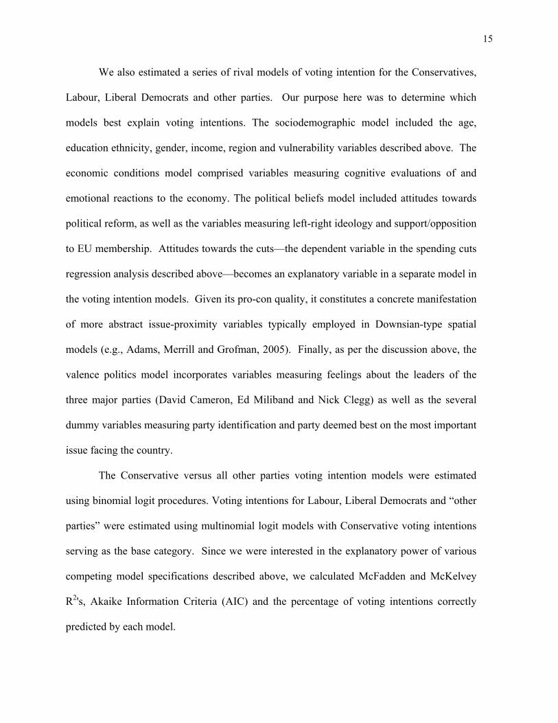
15

We also estimated a series of rival models of voting intention for the Conservatives,

Labour, Liberal Democrats and other parties. Our purpose here was to determine which

models best explain voting intentions. The sociodemographic model included the age,

education ethnicity, gender, income, region and vulnerability variables described above. The

economic conditions model comprised variables measuring cognitive evaluations of and

emotional reactions to the economy. The political beliefs model included attitudes towards

political reform, as well as the variables measuring left-right ideology and support/opposition

to EU membership. Attitudes towards the cuts—the dependent variable in the spending cuts

regression analysis described above—becomes an explanatory variable in a separate model in

the voting intention models. Given its pro-con quality, it constitutes a concrete manifestation

of more abstract issue-proximity variables typically employed in Downsian-type spatial

models (e.g., Adams, Merrill and Grofman, 2005). Finally, as per the discussion above, the

valence politics model incorporates variables measuring feelings about the leaders of the

three major parties (David Cameron, Ed Miliband and Nick Clegg) as well as the several

dummy variables measuring party identification and party deemed best on the most important

issue facing the country.

The Conservative versus all other parties voting intention models were estimated

using binomial logit procedures. Voting intentions for Labour, Liberal Democrats and “other

parties” were estimated using multinomial logit models with Conservative voting intentions

serving as the base category. Since we were interested in the explanatory power of various

competing model specifications described above, we calculated McFadden and McKelvey

R2's, Akaike Information Criteria (AIC) and the percentage of voting intentions correctly

predicted by each model.

16

Of particular interest in the model comparisons is whether attitudes towards the cuts

largely account for the political preferences of voters, or whether the valence politics model

provides greater explanatory power. Our hypothesis is that, even in times of economic crisis,

voters' reactions to policies designed to address such a crisis are a substantial, but secondary,

element in the calculus of electoral choice. Accordingly, we hypothesize that the valence

politics model incorporating party performance on a range of valence issues, partisan

identifications and leader images will outperform a pure 'cuts model' and other rivals. In

addition, based on previous research, we expect that a composite model incorporating the

predictor variables from all five individual models will perform better than any individual

model.

Public Reactions to the Budget Cuts

The May 2011 BES survey data shows that many Britons are not sanguine about the

conditions facing the country. They also are divided about the cause of the crisis and the

policy path to recovery. Specifically, as Figure 1 illustrates, almost half of the respondents

(49 percent) attribute the necessity for spending cuts to mismanagement by the Labour Party

during its tenure in office, with 32 percent disagreeing that Labour policies caused the cuts.

Almost as many (47 percent) agreed that cuts were essential to preserve the long-term health

of the economy. Forty-five percent believed that the policies of the Cameron Government

would cause difficulties for their households whereas only 20 percent disagreed. Thirty-five

percent said they did not know what the personal impact of the cuts would be.

(Figure 1 about here)

Regarding assessments of the cause of Britain’s public debt, there were lower levels

of agreement on whether public excessive spending was the cause. Specifically, 37 percent

17

agreed that public spending was the cause of the debt, but 36 percent disagreed, and 27 were

uncertain. A possible explanation for this division in opinion may be widespread anger over

massive bailouts provided by the government to stabilize British banks. News stories persist

about the anger of Britons towards their banks, as manifested in recent controversies over

bonuses for bank executives who presided over speculative investments and the credit crunch

that followed the meltdown of major financial institutions.

Figure 2 summarizes data on attitudes towards expenditure cuts and the philosophical

balance between government provision of services and personal responsibility. Thirty-six

percent of Britons believe the spending cuts will strengthen the economy and 43 percent

believe the cuts will damage it. But a majority of respondents were skeptical of the

proposition that the government should provide fewer services and rely on individuals to

fend for themselves—55 percent said only the government can provide good public services,

compared to 29 percent who would opt for fewer government services.

(Figure 2 about here)

Tracing the dynamics of these opinions over time was accomplished using identical

questions contained in the monthly Continuous Monitoring Study surveys conducted between

June 2010 and January 2012. During this time frame, the percentage agreeing that the cuts

are essential to Britain’s economic health has fallen from 68 percent to the high 50s (see

Figure 3). In contrast, agreement that the cuts are likely to cause serious personal difficulties

has risen from 41 to 54 percent, while disagreement has fallen from 26 to 19 percent.

Whether excessive public spending was the cause of Britain’s debt produces is a contentious

proposition; public agreement and disagreement has fluctuated across a 10 point range for

18

agreement and a seven-point range for disagreement, but more people continue to agree that

excessive spending is the main cause of the British debt than disagree.

(Figure 3 about here)

Analyzing Attitudes Towards the Budget Cuts

The multivariate model of attitudes towards the cuts specifies 21 predictor variables,

of which 18 are statistically significant (p < .05) (Table 1). The model accounts for 51

percent of the variation in the dependent variable. As expected, party identification proved to

be a powerful predictor of support, with the Conservative identifiers (beta = 0.58) supporting

the cuts. Identifiers with the Liberal Democrats, the Conservatives' occasionally balky

coalition partner, showed more modest support (beta = 0.17). Labour identifiers were

strongly against the cuts, with a coefficient of -0.52.

(Table 1 about here)

Most socio-demographic variables were statistically significant and correctly signed.

Higher income and education, and male gender, produced positive support for the cuts, but

vulnerability (i.e., unemployed, disabled, caregiver), residing in Scotland and advanced age

decreased support for the cuts. The negative coefficient for age suggests that the elderly do

indeed perceive threats to their security from the cuts.

Similarly, most attitudinal variables tapping 'left-right' political orientations of

various kinds performed as expected. Thus, people who support EU membership and those

who emphasize the rights of the accused were less likely to support the cuts than were those

calling for Britain to sever its EU ties and prioritize crime fighting. The three dimensions of

attitudes towards institutional reform also produced the hypothesized results. The greater is

one’s support for traditional institutions—the church, monarchy and Parliament—the greater

19

is the likelihood of supporting the public spending cuts. The same relationship obtains for

those who support devolving more government power to local governments and individuals,

a key component of Mr. Cameron's "Big Society" vision. Again, as also expected, support

for reform of the electoral system is associated with opposition to the cuts. Finally, there is

evidence that more general personality characteristics are relevant, with heightened risk

acceptance being correlated with increased support for the cuts.

Analyzing Support for the Conservatives and David Cameron

Table 2 reports the results of estimating composite models of Conservative vote

intentions and feelings about Prime Minister Cameron, the chief proponent (with Chancellor

George Osborne) of the public spending cuts. After party identification and the judgment

that a Conservatives are best on the most important issue, support for public spending cuts is

the strongest predictor of affect for Cameron. The composite model explains 62 percent in

the variance in feelings about the prime minister, and estimates of coefficients for 17 of 24

predictor variables are statistically significant. All party identification terms are significant

predictors, as are all of the judgments on which party is best able to handle the most

important issue.

As noted above, we estimate the effects of factors affecting Conservative vote

intentions using a binomial logit model. This composite model correctly classifies 93.4

percent of the vote intentions and generates a McKelvey R2 of .87. To provide intuition

about the strength of the effects of various independent variables, we also estimated changes

in probability of voting Conservative as statistically significant predictors were varied over

their range while holding other predictors at their mean values in the case of continuous

variables or zero in the case of dummy variables. This procedure showed that the predicted

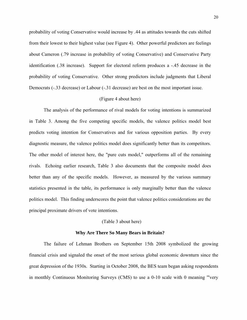
20

probability of voting Conservative would increase by .44 as attitudes towards the cuts shifted

from their lowest to their highest value (see Figure 4). Other powerful predictors are feelings

about Cameron (.79 increase in probability of voting Conservative) and Conservative Party

identification (.38 increase). Support for electoral reform produces a -.45 decrease in the

probability of voting Conservative. Other strong predictors include judgments that Liberal

Democrats (-.33 decrease) or Labour (-.31 decrease) are best on the most important issue.

(Figure 4 about here)

The analysis of the performance of rival models for voting intentions is summarized

in Table 3. Among the five competing specific models, the valence politics model best

predicts voting intention for Conservatives and for various opposition parties. By every

diagnostic measure, the valence politics model does significantly better than its competitors.

The other model of interest here, the "pure cuts model," outperforms all of the remaining

rivals. Echoing earlier research, Table 3 also documents that the composite model does

better than any of the specific models. However, as measured by the various summary

statistics presented in the table, its performance is only marginally better than the valence

politics model. This finding underscores the point that valence politics considerations are the

principal proximate drivers of vote intentions.

(Table 3 about here)

Why Are There So Many Bears in Britain?

The failure of Lehman Brothers on September 15th 2008 symbolized the growing

financial crisis and signaled the onset of the most serious global economic downturn since the

great depression of the 1930s. Starting in October 2008, the BES team began asking respondents

in monthly Continuous Monitoring Surveys (CMS) to use a 0-10 scale with 0 meaning '"very

21

unlikely" and 10 meaning "very likely" to forecast the likelihood that the crisis would be

resolved over the year ahead. From the outset, CMS respondents were quite bearish, with their

average score being 4.0 on the scale. Moreover, as illustrated in Figure 5, their pessimism has

grown over time, such that the average score in January 2012, is only 2.1. Since the

Conservative-Liberal Democrat Coalition took office, the average score has never exceeded 3.0.

(Figure 5 about here)

What are the sources of this pessimism? A simple answer to this question is: "It's

reality!—people are bearish because the economy is in terrible shape and shows little, if any,

sign of reviving." Given a continuing barrage of bad news about economic conditions, it is not

surprising that many people are less than sanguine about that the crisis will be resolved anytime

soon. In this regard, perhaps no single indicator carries as much weight in the public mind as the

unemployment rate—it is effectively an operational definition of how hard times are. In this

regard, Figure 5 documents that UK unemployment has risen from 5.8 percent in October 2008

to 8.4 percent in January 2012, with modest decreases in the run-up to the 2010 election being

followed by upward movements throughout much of 2011. The correlation between

expectations of solving the crisis and the unemployment rate is strongly negative ( r = -.67).

If, in fact, people typically use unemployment as the "big heuristic" for assessing the

present state and future prospects of the economy, then we should be able to model the

relationship between forecasts for solving the crisis and the jobless rate as an error correction

process. Other factors may have transient relevance for explaining variation in these forecasts,

but over the long run, they should evolve in dynamic equilibrium with movements in the length

of lines at Jobs Centers. Here, we specify three such factors. The first is Chancellor George

Osborne's annual budget speeches in 2009, 2010 and 2011 which have delivered a largely

22

unrelieved litany of bad news about the need for varying mixtures of spending cuts and tax hikes.

Second is the March 2009 announcement by the former Labour government of a massive and

unprecedented quantitative easing program to jump start the faltering economy. Third is the

presence since May 2010 of the Conservative-Liberal Democrat Coalition Government. Prime

Minister Cameron and Chancellor the Exchequer, George Osborne, have made the ailing

economy and an attendant need for austerity the touchstone of virtually every policy proposal

advanced by the Coalition Government. As a result, most of what passes for daily political news

includes a reminder that times are indeed tough. And, for their part, Labour Leader, Ed

Miliband, and his Shadow Chancellor, Ed Balls, have countered by claiming that the hard times

are worse than need be because their opposite numbers insist on pursuing an ill-advised neo-

Thatcherite economic agenda. In their view, privileging Hayek over Keynes is a recipe risks

rehearsing the 1930s.

The resulting model of public forecasts for whether the economic crisis will be resolved

over the forthcoming year is:

(1-L)RESOLVE(t) = b0 + b1*(1-L)UN(t-i) - α1*(RESOLVE(t-1) - λ1*UN(t-1)) +

b2*BUDGET(t-i) + b3*QE(t-i) + b4*COAL(t-i) + ε(t) (1)

where: RESOLVE = forecast for resolving the economic crisis; UN = unemployment rate;

BUDGET = annual budgets; QE = quantitative easing; COAL = Coalition government; εt =

stochastic error term (N (0,σ2), t is time, and α, b and λ are parameters to be estimated. Given

the structure of the model, its parameters are estimated using nonlinear least squares.

Results of analyzing the model using data for the October 2008 - January 2012 period are

displayed in Table 4. As shown, the model can account for a large percentage of the variation in

public forecasts for resolving the economic crisis (adjusted R2 = .64) and all parameters are

23

statistically significant and properly signed. Indicative of the power of the error correction

mechanism between these forecasts and monthly unemployment, the adjustment parameter is

-.74, p < .001. This signifies that a shock to the system, from whatever source, is eroded at a rate

of nearly 75 percent in each subsequent month by the error correction relationship between

forecasts for resolving the crisis and the unemployment rate. Unemployment also has large

short-term effects, with a one per cent increase in joblessness being sufficient to lower forecasts

by nearly one full point (-.95) on the 0-10 scale.

(Table 4 about here)

Other factors are in play as well. As expected, annual budgets, the March 2009 round of

quantitative easing, and the replacement of Labour by the Coalition all worked to lower public

forecasts of the likelihood that the economic crisis would be resolved over the next year. The

impact of the presence of the Coalition government is especially noteworthy. Specified as a

(thus far) permanent effect, the presence of the Coalition has worked (ceteris paribus) to reduce

economic forecasts by -.71 points each month. Effects of annual budget statements and

quantitative easing are smaller, .-15 and -.43, respectively, but statistically significant (p < .001).

Overall, the model provides a parsimonious account of public forecasts about the future

course of the economic crisis. As hypothesized, unemployment is the key heuristic, with

forecasts and joblessness defining a powerful error correction process. Since the autumn of

2008, that process has adjusted the effects of various political economic shocks, the largest being

the replacement of Labour by the Conservative-Liberal Democrat coalition at Westminster.

Conclusion: Economic Crisis and Performance Politics

David Cameron and his Coalition colleagues have chosen to ride the tiger of the poor

economic times while attempting to enact public spending cuts that trade pain today with the

24

promise of gain tomorrow. As the anti-Wimpy (Popeye’s sidekick sought a hamburger today for

payment tomorrow), the prime minister demands payment today and promises a hamburger

tomorrow. To date, Cameron has successfully tapped British public opinion that acknowledges

the seriousness of budgetary and sovereign debt difficulties and the need to address endemic

fiscal problems. Support for the Coalition's budget cuts is tied to party identification, economic

evaluations and reactions, and demographic factors that indicate self-sufficiency. But factors

that suggest economic vulnerability—unemployment, aging and lack of education and income—

mitigate the willingness to jump head first into schemes to shrink government.

Although there is a strong partisan divide in attitudes toward the cuts, Mr. Cameron and

his friends on the government benches face mounting skepticism on several fronts. First, there is

substantial fear that the cuts could damage the economy instead of curing it, and that the cuts

could cripple government infrastructure required to provide public services effectively. Second,

the uncertainty of policy outcomes and a changing economic environment means the cuts,

however well conceived in 2010 and 2011, may not be seen as effective policy going forward

and will prove to be a political liability in the run-up to the next general election. Open-ended

responses to the question in the BES AV referendum survey about the most important issue

facing the country are suggestive with regard to the latter possibility. Many of these responses

acknowledge the need of fiscal restraint, but others reject the present program as “too far, too

fast.” Still others raise equity-fairness concerns which could gain traction in the face of

disappearing benefits and services and continuing economic malaise.

A third, more pointed, element of skepticism recently has been enunciated as medical

professionals, interest groups and concerned patients attempt to rein in government plans to

restructure the cherished National Health Service. Since the Conservative-Liberal Democrat

25

Coalition came to power, commentators in the British press have asked whether a single-minded

pursuit of deep spending cuts is the right policy at the right time. Now they are asking if Prime

Minister Cameron and his much maligned Health Secretary Andrew Lansley are privileging a

Thatcherite ideological agenda at the expense of effective health care delivery.

Analyses of CMS time series data suggest that public support for the cuts eventually may

be undermined by a lack of visible results in the real economy. Although cuts currently are

widely perceived as essential for Britain's long-term economic health, an upward trending view

that slashing public services will cause serious difficulties for families may lead many people to

say enough is enough. Sustained high levels of unemployment propelled by public sector job

cuts put mounting pressure on relief programs and are unlikely to be regarded kindly by either

frustrated job seekers or those who used to be served by the fired employees. Furthermore,

confidence in the nation’s ability to solve the economic crisis has been falling as unemployment

continues to rise. At some point, public spending cuts may seem an inappropriate, unjust and

harsh response to a problem that is increasingly viewed as intractable to short-term solutions.

Finally, the fact that valence politics variables do much to drive the composite vote

intention model indicates that attitudes toward the spending cuts will not be the sole drivers of

party support in the next general election. Rather than respond directly and reflexively to the

conditions around them, British voters place economic hardships and policy in broader context

with images of party leaders, partisan attachments and more global assessments of party

performance. Differing attitudes about the harsh austerity measures are exerting substantial

effects on party support, but these attitudes have not negated the force of valence politics

considerations. Rather, reactions to the evolving state of the economy coupled with mutable

partisan attachments and the more general evaluations of party and leader performance that

26

voters are making can be expected to animate the model in predictable ways in the years ahead.

Performance politics remains important for understanding electoral choice in Britain and other

mature democracies as the present era of economic hardship and austerity policies unfolds.

27

ENDNOTES

1. The question format for the first three components of the dependent variable was as follows: Please indicate how far you agree or disagree with each of the following statements: - The Government’s cuts in public expenditure are essential for the long-term

health of the UK economy. - The cuts in public expenditure that the Government proposes are likely to

cause serious financial difficulties for me and my family. - Excessive public spending is the main cause of Britain’s debt.

Respondents could choose between Strongly approve, Approve, Neither approve nor disapprove, Disapprove, Strongly disapprove or Don’t know. The fourth question stated: Which of the following statements come closest to your view about the overall impact of the proposed public expenditure cuts?

- The public expenditure cuts will strengthen Britain’s economic growth and international competitiveness.

- The public expenditure cuts will damage Britain’s economy by pushing it further into recession.

- Don’t know. The fifth question was worded thus: Which of the following statements comes closest to your view?

- The government should do less to provide publicly funded services and do more to encourage people to provide services for themselves.

- Good public services can be provided only by the government. - Don’t know.

2. Respondents were asked to evaluate seven statement on five-point Likert scales: - The House of Commons should be reduced to 600 members. - The electoral system should be changed to proportional representation. - Local governments should have more authority. - The Monarchy should be abolished. - The Church of England should keep its status. - The United Kingdom needs more referendums to decide important issues. - MPs who vote against the party manifesto should resign and run again for their seats. The pre-wave question asked the respondents to designate which statement was more important:

- That one party get more than half the vote so it can govern on its own. - That every party’s percentage of seats in Parliament is the same as their

percentage of the vote. - Don’t know.

28

.

29

Figure 1

Source: 2010 BES-CMS AV referendum survey

.

Opinions About Cuts in Public Expenditure

47

49

45

37

23

19

35

27

30

32

20

36

0% 10% 20% 30% 40% 50% 60% 70% 80% 90% 100%

Cuts Essential forLong-Term Health of

Economy

Cuts Due to LabourMismanagement

Cuts Cause PersonalDifficulty

Excessive PublicSpending CausedGovernment Debt

Agree Neither/DK Disagree

30

Figure 2

Opinions About Budget Cuts and Public Services

3643

2129

55

16

0

20

40

60

80

100

CutsStrengthenEconomy

CutsDamage

Economy

Don't Know GovernmentShouldProvide

Fewer PublicServices

OnlyGovernmentCan ProvideGood Public

Services

Don't Know

Per

cen

t

Source: 2010 BES-CMS AV referendum survey .

31

Figure 3

Dynamics of Public Opinion About Cuts in Public Expenditure October 2008 - January 2012

10

20

30

40

50

60

06 07 08 09 10 11 12 01 02 03 04 05 06 07 08 09 10 11 12 012010 2011 2012

Per

cen

t

Date

Agree

Disagree

41

25

54

19

Percentages Agreeing or Disagreeing that Cuts are LikelyCause Serious Difficulties for Themselves and Their Families

10

20

30

40

50

60

70

06 07 08 09 10 11 12 01 02 03 04 05 06 07 08 09 10 11 12 012010 2011 2012

Per

cen

t

Date

Agree

Disagree

68

12

56

22

Percentages Agreeing or Disagreeing that Cuts are Essentialfor Long-Term Health of the UK Economy

25

30

35

40

45

50

06 07 08 09 10 11 12 01 02 03 04 05 06 07 08 09 10 11 12 012010 2011 2012

Per

cen

t

Date

Agree

Disagree

45

31

40

33

Percentages Agreeing or Disagreeing that Excessive Public SectorSpending is Main Cause ofBritain's Debt

Source: June 2006 - January 2012 BES-CMS surveys.

32

Figure 4

Change in Probability of Intending to Vote Conservative Associated With

Statistically Significant Predictors in Binomial Logit Model

33

Figure 5

2.0

2.4

2.8

3.2

3.6

4.0

4.4

5.5

6.0

6.5

7.0

7.5

8.0

8.5

08 10 01 04 07 10 01 04 07 10 01 04 07 10 01

2008 2009 2010 2011 2012

UnemploymentRate

Solve FinancialCrisis Next Year

Like

lihoo

d So

lve

Fina

ncia

lC

risis

Nex

t Yea

r (0-

10 S

cale

)U

nemploym

entRate

r = -.67

4.0

5.8

8.4

2.1

Date

2010 General Election-->

Likelihood of Solving Financial Crisis Next Yearand Unemployment Rate, August 2008 - January 2012

Source: October 2008 - January 2012 BES-CMS surveys and ONS unemployment data. .

34

Table 1. Multivariate Model of Opinions About Cuts in Public Expenditure,

May 2010 BES-AV Survey (OLS Estimates)

Predictor Variable B s.e. Party Identification: Labour -.518*** .015 Conservative .581*** .016 Liberal Democrat .174*** .021 Other Party -.007 .020 Economic Evaluations .264*** .007 Emotional Reactions Economic Conditions .074*** .004 Ideological/Policy Beliefs: Attitudes Towards Reform: Electoral System -.986*** .006 Devolution of Power .063*** .006 Traditional Institutions .091*** .006 Crime v. Rights of Accused -.023*** .002 EU Membership -.073*** .005 Risk Orientation .012*** .002 Vulnerability Status† -.061** .019 Age -.004* .002 Age Squared 9.334E-05*** 2.406E-05 Education .018*** .004 Ethnicity .009 .024 Gender .067*** .011 Income .022*** .002 Scotland -.032* .019 Wales -.009 .238 Constant .045 .061 Adjusted R2 = .51 N = 18,556 *** - p < .001; ** - p < .01; * - p < .05, one-tailed test. † - Unemployed, disabled, care-giver

35

Table 2. Multivariate Models of Conservative Vote Intentions and Feelings About Prime Minister David Cameron, May 2010 BES-AV Survey

Conservative Feelings About Vote Intentions† David Cameron‡ Predictor Variables B s.e. B s.e. Opinions About Public Expenditure Cuts .604*** .059 .974*** .021 Feelings About: David Cameron .516*** .025 -- -- Ed Miliband -.152*** .021 -- -- Nick Clegg -.140*** .022 -- -- Party Identification: Labour -1.776*** .134 -.573*** .046 Conservative 2.065*** .110 1.351*** .050 Liberal Democrat -1.774*** .140 .356*** .061 Other Party -1.628*** .129 -.222*** .057 Party Best Most Important Issue: Labour -1.867*** .255 -.709*** .046 Conservative .887*** .099 1.204*** .046 Liberal Democrat -2.098*** .412 .216* .093 Other Party -1.088*** .129 -.287*** .052 Economic Evaluations .079 .051 .166*** .019 Emotional Reactions to Economic Conditions .022 .030 .206*** .011 Ideological/Policy Beliefs: Attitudes Towards Reform: Electoral System -.479*** .044 -.089*** .016 Devolution of Power -.053 .045 .005 .015 Traditional Institutions .115** .047 .309*** .016 Crime v. Rights of Accused -.020 .019 -.003 .007 EU Membership -.091* .040 .027* .014 Vulnerability Status -.004 .152 -.067 .051 Age -.012*** .003 .006*** .001 Education -.080** .032 -.007 .011 Ethnicity .235 .183 .033 .064 Gender -.358*** .083 -.187*** .029 Income .027* .017 .003 .005 Scotland -.704*** .157 -.010 .051 Wales -.685*** .191 .153** .065 Constant -.968*** .310 4.161*** .097 McKelvey R2 = .87 Percentage Correctly Classified = 93.4 Adjusted R2 = .62 N = 18,556 -- - variable not included in model. † - binomial logit model. ‡ - OLS regression model.

36

Table 3. Rival Models of Voting Intentions, May 2011 CMS Survey Panel A. Conservative Voting Intentions (Binomial Logit Model) Percent Correctly Model McFadden R2 McKelvey R2 Classified AIC†

Socio-demographics .04 .06 64.6 19052.93 Economic Conditions .10 .17 69.0 17708.06 Political Beliefs .17 .29 72.3 16479.42 Attitudes-Cuts .38 .54 80.9 12309.00 Valence Politics‡ .76 .86 93.8 4829.82 Composite .77 .87 94.4 4506.15 Panel B. Labour, Liberal Democrat and Other Party Voting Intentions (Multinomial Logit Model) Percent Correctly Model McFadden R2 McKelvey R2 Classified AIC†

Socio-demographics .04 -- 44.7 36445.06 Economic Conditions .07 -- 51.6 35014.82 Political Beliefs .14 -- 53.8 32513.98 Attitudes-Cuts .25 -- 66.7 28238.60 Valence Politics‡ .70 -- 87.2 11344.86 Composite .72 -- 88.2 10634.37 † - Akaike Information Criterion; smaller values indicate better model performance (Burnham and Anderson, 2002). ‡ - leader images, party identification, party best on most important issue. -- - not defined for multinomial logit model.

37

Table 4. Error Correction Model of Dynamics of Opinions Whether the Financial Crisis Will Be Resolved in Year Ahead,

October 2008 - January 2012 Predictor Variables B s.e. Change in Unemployment Rate (t-1) -.954*** .022 Error Correction Mechanism -.743*** .103 Unemployment Rate (t-1)- ECM -.289*** .071 2009-2011 Budget Statements -.146* .087 2009 Quantitative Easing -.426** .149 2010 General Election -.712*** .102 Constant 4.172*** .744 Adjusted R2 = .64 N = 39 *** - p < .001; ** - p < .01; * - p < .05, one-tailed test. Residual Diagnostics: Autocorrelation: LBQ = 9.967, df = 12, p = .619 ARCH: LBQ = 7.339, df = 12, p = .834 Normality: Jarque-Bera = .573, df = 1, p = .751 Heteroskedasticity: χ2 = 5.119, df = 6, p = .529

38

REFERENCES Achen, Christopher H. 1992. Social Psychology, Demographic variables, and Linear Regression: Breaking the Iron Triangle in Voting Research. Political Behavior 14 (3): 195-211. Adams, James, Samuel Merrill III and Bernard Grofman. 2005. A Unified Theory of Party Competition. Cambridge: Cambridge University Press. Bartels, Larry. 2008. Unequal Democracy: The Political Economy of the New Gilded Age. Princeton: Princeton University Press. Berelson, Bernard R., Paul F. Lazarsfeld and William N. McPhee. 1954. Voting. Chicago: The University of Chicago Press. Bloomberg.com. 2011. U.K. Needs Cameron’s Austerity, but Perhaps Not So Quickly: View. Dec. 11: http://www.bloomberg.com/news/2011-12-07/u-k-needs-cameron-s-austerity- program-but-perhaps-not-so-quickly-view.html. Accessed Feb. 24, 2012. Borre, Ole. and Jose Manuel Viegas. 1995. Government Intervention in the Economy, pp. 234- 280 in The Scope of Government, ed. Ole Borre and Elinor Scarbrough. Oxford: Oxford University Press. British Broadcasting Corp. 2011. EU Austerity Drive Country by Country. Nov. 11: http://www.bbc.co.uk/news/10162176. Accessed Feb. 24, 2012. British Election Study. 2011. AV Ballot Referendum Study. Colchester: University of Essex. British Election Study. 2012. Continuous Monitoring Surveys, June 2010 - January 2012. Colchester: University of Essex. Burns, John F. 2011. British Leader Pushes for ‘Can-Do Optimism’ and Faith in Austerity Path. New York Times. Oct. 6: A10. Butler, David and Donald E. Stokes. 1969. Political Change in Britain. New York: St. Martin's Press. Campbell, Angus, Philip E. Converse, Warren E. Miller, and Donald E. Stokes. 1960. The American Voter. New York: Wiley. Clarke, Harold D., Allan Kornberg, and Thomas J. Scotto. 2009. Making Political Choices: Canada and the United States. Toronto: University of Toronto Press. Clarke, Harold D. and Allan McCutcheon). 2009. "The Dynamics of Party Identification Revisited." Public Opinion Quarterly 73: 704-28.

39

Clarke, Harold D., David Sanders, Marianne C. Stewart and Paul Whiteley. 2004. Political Choice in Britain. Oxford: Oxford University Press. Clarke, Harold D., David Sanders, Marianne C. Stewart and Paul Whiteley. 2009. Performance Politics and the British Voter. Cambridge: Cambridge University Press. Confalonieri, Maria A., and Kenneth Newton. 1995. Taxing and Spending: Tax Revolt or Tax Protest. pp 121-14, in The Scope of Government, ed. Ole Borre and Elinor Scarbrough. Oxford: Oxford University Press. Cutler, Fred. 2002. The Simplest Shortcut of All: Sociodemographic Characteristics and Electoral Choice. The Journal of Politics. 64: 466-90. Dalton, Russell J. 2006. Citizen Politics, 4th ed. Washington: CQ Press. Downs, Anthony. 1957. An Economic Theory of Democracy. New York: Harper and Row. Downs, Anthony. 1960. Why the Government Budget is Too Small in a Democracy. World Politics. 12(4): 541-63. Easton, David. 1965. A Systems Analysis of Political Life. New York: Wiley. Fiorina, Morris P. 1981. Retrospective Voting in American National Elections. New Haven: Yale University Press. Kornberg, Allan, and Harold D. Clarke. 1992. Citizens and Community: Political Support in a Representative Democracy. Cambridge: Cambridge University Press. Kumlin, Staffan. 2007. The Welfare State: Values, Policy Preferences, and Performance Evaluations, in The Oxford Handbook of Political Behavior. Oxford: Oxford University Press. Lazarsfeld, Paul F., Bernard Berelson and Hazel Gaudet. 1944. The People’s Choice. New York: Duell, Sloan and Pearce. Lewis-Beck, Michael S. 1988. Economics and Elections: The Major Western Democracies. Ann Arbor: University of Michigan Press. Lewis-Beck, Michael S., Richard Nadeau and Eric Bélanger. French Presidential Elections. London: Palgrave Macmillan, 2011. Lewis-Beck, Michael S., and Mary Stegmaier. 2000. Economic Determinants of Electoral Outcomes. Annual Review of Political Science. 3: 183-219.

40

Lewis-Beck, Michael S., William G. Jacoby, Helmut Norpoth and Herbert F. Weisberg. 2008. The American Voter Revisited. Ann Arbor: The University of Michigan Press. Lupia, Arthur, and Mathew D. McCubbins. 1998. The Democratic Dilemma: Can Citizens Learn What They Need to Know? New York: Cambridge University Press. Pierson, Paul, ed. 1993. The New Politics of the Welfare State. Oxford: Oxford University Press. Sniderman, Paul M., Richard A. Brody, and Philip Tetlock. 1991. Reasoning and Choice: Explorations in Political Psychology. Cambridge: Cambridge University Press. Stokes, Donald E. 1963. Spatial Models of Party Competition. American Political Science Review 57(2): 368-377. Stokes, Donald E. 1992. Valence Politics. In Electoral Politics, edited by D. Kavanagh. Oxford: Clarendon Press. Werdigier, Julia. 2011. Its Growth Slowing, Britain Extends Austerity Measures. New York Times. Nov. 30: B8. Winter, Soren, and Poul Erik Mouritzen, PE. 2001 Why people Want Something for Nothing: The Role of Asymmetrical Illusions. European Journal of Political Research. 39: 109- 43.

Modeling Elections with Varying Party Bundles:

Applications to the 2004 Canadian Election

Kevin McAlister, Jee Seon Jeon, & Norman Scho�eld

September 29, 2012

1 Introduction

Early work in formal political theory focused on the relationship between constituencies

and parties in two-party systems. It generally showed that in these cases, parties had

strong incentive to converge to the electoral median (Hotelling, 1929; Downs, 1957; Riker

and Ordeshook, 1973). These models assumed a one-dimensional policy space and non-

stochastic policy choice, meaning that voters would certainly vote for a party. These

models showed that there exists a Condorcet point at the electoral median. However,

when extended into spaces with more than one dimension, these two-party pure-strategy

Nash equilibria generally do not exist. While attempts were made to reconcile this di¤er-

ence, the conditions necessary to assure that there is a pure-strategy Nash equilibrium at

the electoral median were strong and unrealistic with regards to actual electoral systems

(Caplin and Nalebu¤, 1991).

Instead of pure-strategy Nash equilibria (PNE) there often exist mixed strategy Nash

equilibria, which lie in the subset of the policy space called the uncovered set (Kramer,

1978). Many times, this uncovered set includes the electoral mean, thus giving some

credence to the median voter theorem in multiple dimensions (Poole and Rosenthal, 1984;

Adams and Merrill, 1999; Merrill and Grofman, 1999; Adams, 2001). However, this seems

at odds with the chaos theorems which apply to multidimensional policy spaces.

The contrast between the instability theorems and the stability theorems suggest that

2

a model in which the individual vote is not deterministic is most appropriate (Scho�eld,

Martin, Quinn and Whitford, 1998; Quinn, Martin and Whitford, 1999). This kind of

stochastic model states that the voter has a vector of probabilities corresponding to the

choices available in the election. This insinuates that if the voter went to the polls for the

same election multiple times, he might not make the same vote every time. This model

is in line with multiple theories of voter behavior and still yields the desirable property of

showing that rational parties will converge to the electoral mean given the simple spatial

framework.

Using this framework, Scho�eld(2007) shows that convergence to the mean need not

occur given that valence asymmetries are accounted for. In this context, valence is taken

to mean any sorts of quality that a candidates has that is independent of his location

within a policy space. In general, valence is linked to the revealed ability of a party to

govern in the past or the predicted ability of a party to govern well in the future. In recent

years, models with a valence measure have been developed and utilized in studies of this

sort. Scho�eld extends upon these models and demonstrates a necessary and su¢ cient

condition for convergence to the mean, meaning that the joint electoral mean is a local

pure-strategy Nash equilibrium (LNE) in the stochastic model with valence.

Valence can generally be divided into two types of valence: aggregate valence (or

character valence) and individual valence (or sociodemographic valence). Both types of

valence are exogenous to the position that a party takes in an election, meaning that

these valence measures rely on some other underlying characteristic. Aggregate valence

is a measure of valence which is common to all members in an electorate, and can be

interpreted as the average perceived governing ability of a party for all members of an

electorate (Penn, 2003). Individual valence is a bit more speci�c, where this kind of valence

depends upon the characteristics of a voter. This kind of valence di¤ers from individual

to individual. For example, in United States elections, African-American voters are very

much more likely to vote for the Democratic candidate than they are to vote for the

Republican candidate. Thus, it can be said that the Democratic candidate is of higher

valence among African-American voters than the Republican candidate is. Both kinds of

valence can be important in determining the outcomes of elections and are necessary to

3

consider when building models of this sort.

Recent empirical work on the stochastic vote model has relied upon the assumption

of Type-I extreme value distributed errors (Dow and Endersby, 2004). These errors,

commonly associated with microeconometric models, are typical of models that deal with

individual choice, where individual utility is determined by the valence terms and the

individual�s distance from the party in the policy space. This distance is weighted by �, a

constant that is determined by the average weight that individuals give to their respective

distances from the parties. The workhorse of individual choice models is the multinomial

logit distribution, which is an extension of the dichotomous response logit distribution.

This distribution assumes that the probability that an individual votes for a party follows

the Type-I extreme value distribution, thus matching the assumed distribution of the

stochastic voting model. This creates a natural empirical partner for the stochastic vote

model.

Using this statistical framework and the assumption that individual choice follows this

distribution, Scho�eld(2007) introduced the idea of the convergence coe¢ cient, c, which

is a measure of attraction to the electoral mean in an electoral system. This coe¢ cient is

unitless, thus it can be compared across models. Low values of this value indicate strong

attraction to the electoral mean, meaning that the electoral mean is a local pure-strategy

Nash equilibrium (Patty, 2005; Patty, 2006). High values indicate the opposite. He also

lays out a necessary and a su¢ cient condition for convergence to the electoral mean with

regards to the convergence coe¢ cient:

1. When the dimension of the policy space is 2, then the su¢ cient condition for con-

vergence to the electoral mean is c < 1.

2. The necessary condition for convergence is if c < w, where w is the number of

dimensions of the policy space of interest.

When the necessary condition fails, at least one party will adopt a position away from

the electoral mean in equilibrium, meaning that a LNE does not exist at the electoral

mean. As a LNE must exist for the point to be a pure strategy equilibrium, this implies

non-existence of a PNE at the center. Given the de�nition of the convergence coe¢ cient,

4

the general conclusion is that the smaller � is, the smaller the valence di¤erences are

among candidates, and the lower the variance of the electoral distribution is, the more

likely there is to be a LNE at the electoral center.

However, this only answers the question where the local Nash equilibria are in the

simplest case of having one electoral mean that parties are responding to. This problem can

quickly become more complicated. Imagine a country with �ve parties and two di¤erent

regions. Four of the parties run in both regions, and are thus attempting to appeal to

voters in both regions. However, one of these parties only runs in one of the regions and

is only trying to appeal to the voters of this region. Thus, it would be unreasonable for

it to position itself with regards to the electoral mean for the entire electorate. Rather, it

wants to maximize its vote share within in the region in which it runs. Parties can choose

to run in select regions for a variety of reasons. They may run for historical reasons or

responsive reasons or even choose not to run in regions where they know they will not

do well at all. As parties have limited resources, sometimes this kind of decision must be

made.

In order to assess convergence to the electoral mean in this case, one must take into

account the electoral centers that parties are responding to. In the above example, con-

vergence to the electoral mean would mean that the �rst four parties converge to the

overall electoral mean, or the mean of all voters in the electorate, while the �fth party

would converge to the electoral mean of those individuals in its respective region. Thus,

the convergence coe¢ cient would no longer be appropriate, as it is proven only when the

position for all parties is equal to zero on all dimensions. Similarly, when there are par-

ties which run in di¤erent combinations of regions, the typical multinomial logit model is

no longer appropriate because the underlying assumption of "independence of irrelevant

alternatives"(IIA) is no longer met (Train, 2003). Given that there are problems with

estimation of parameters from the currently utilized empirical methodology and problems

with the underlying theoretical mechanism that drives the reasoning behind the conver-

gence coe¢ cient, we are left without the useful information gained about party tendencies

in the stochastic model. Under the current framework, researchers can only analyze con-

vergence, valence, and spatial adherence within speci�c regions. However, in this paper

5

we propose a method for handling more structurally complex electorates.

In this chapter, we introduce methods for analyzing the stochastic vote model in elec-

torates where individuals do not all vote for the same party bundle. First, this chapter will

demonstrate that the convergence coe¢ cient �rst de�ned by Scho�eld can be adjusted to

handle any vector of party positions. We will determine the �rst and second order condi-

tions necessary to show that a vector of policy positions is a local Nash equilibrium (LNE).

From this, we will show that the convergence coe¢ cient for a more complex electorate can

be derived in a similar manner to that used previously. We will also show the necessary

and su¢ cient conditions for convergence. Secondly, we will introduce a method that can

be used to estimate the parameters necessary to �nd equilibria in the model. This empir-

ical model, an extension of the mixed logit model, will utilize the same Type-I extreme

value distribution assumptions used previously, but will not rely upon the IIA assumption

necessary to use the basic multinomial logit model. This varying choice set logit (VCL:

see Yamamoto, 2011) will allow for aggregate estimation of parameters to occur while

also allowing regional parameters to be estimated. This method of estimation along with

the notions of convergence that will allow analysis of the stochastic voting model in more

complex situations.

Finally, to illustrate these methods, we will analyze the Canadian elections in 2004.

Canada has a regional party which only runs in one region of the country, however, in

2004, the regional party gained seats in the Parliament. As this election is an ideal testing

point for these new methods, they can tell us whether or not these new methods give

logical results. From this analysis, some insight can be gained as to the way in which

parties can organize themselves to maximize the number of votes received.

2 The Formal Stochastic Model

The data in the spatial model is distributed xi 2 X where i 2 N represents a member of

the electorates�s ideal point and n is the number of members in the sample. We assume

that X is an open convex subset of Euclidian space, Rw, where w is �nite and corresponds

to the number of dimensions selected to represent the policy space.

6

Each of the parties, j 2 P , where P = f1; :::; j; :::; pg chooses a policy, zj 2 X, to

declare to the electorate prior to the election. Let z = (z1; z2; :::; zp) be the vector of party

positions. Given z, each voter i is described by a vector:

ui(xi; z) = (ui1(xi; z1); ui2(xi; z2); :::; uip(xi; zp))

where uij(xi; zj) = u�ij(xi; zj) + �ij

and u�ij(xi; zj) = �j � �kzj � xik2 + �ij

Here, u�ij(xi; zj) is the observable utility for i, associated with party j. �j is an exoge-

nous valence term for agent j which is common throughout all members of a population

(i.e. party quality)1. � is a positive constant and k:k is the Euclidian distance between

individual i and party j 2. �ij is an exogenous sociodemographic valence term, meaning

that this term can be viewed as the average assessment of a party�s governing ability to

the members of a speci�c group3. The error term, �ij is assumed to be be commonly

distributed among individuals. In particular, we assume that the cumulative distribution

of the errors follows a Type-I extreme value distribution. This is not only the norm in in-

dividual choices, it also allows the theoretical model to match the corresponding empirical

model, making the transition between the two easier.

Given the stochastic assumption of the model, the probability that i votes for j given

z, �ij(z) is equal to:

�ij(z) = Pr[uij(xi; zj) > uil(xi; zl);8l 6= j1This can be conceptualized as an average assessment of the parties quality to govern among all members

of the electorate, regardless of sociodemographic identity.2To match up with the empirical applications later in the paper, the utility individual i gains from

having party j in o¢ ce is compared to a base party, j = 1. As is normal, we assume this party has a utilityof zero and the other utilities are compared to this party. Thus, the utility gained by i by voting for j

can also be seen as u�ij(xi; zj) = �j � �(wX

m=1

((xjm � xim)2 � (x1m� xim)2)) +�ij where the summation is

of the Euclidian distances for each dimension of the policy space. This places our model in line with thelatent utility models that are commonly used in microeconometric theory and bridges the gap between ourtheoretical model and the corresponding empirical model.

3 In this paper, we assume that this term is common among all members of a speci�c sociodemographicgroup. However, we can set up these terms to represent individuals with individual level random e¤ects.

7

In turn, we assume that the expected vote share for agent j given z, is Vj(z) where:

Vj(z) =1

n

X8i2N

�ij(z)

We assume in this model that agent j chooses zj to maximize Vj(z) given the positions

of the other parties. We seek equilibria of the model where each of the parties attempts

to maximize vote share .

For the purposes of this paper, when we talk about an equilibria, we refer to a local

Nash equilibria (LNE). This de�nition of equilibrium relies on maximizing the expected

vote share gained by a party given the positions of the other parties. A vector of positions,

z�, is said the be a LNE if 8j, z�j is a critical point of the vote function and the Hessian

matrix of second derivatives is non-positive , meaning that the eigenvalues are all non

positive. More simply put, a vector, z�, is a LNE if each party locates itself at a local

maximum in its respective vote function. This means, that given the opportunity to make

moves in the policy space and relocate its platform, no vote-maximizing party would

choose to move. We assume that parties can estimate how their vote shares would change

if they marginally move their policy position. The local Nash equilibrium is that vector

z of party positions so that no party may shift position by a small amount to increase its

vote share. More formally a LNE is a vector z = (z1; :::; zj ; :::; zp) such that each Vj(z)

is weakly locally maximized at the position zj . To avoid problems with zero eigenvalues

we also de�ne a strict local Nash equilibrium (SLNE) to be a vector that strictly locally

maximizes Vj(z). We typically denote an LNE by z(K) where K refers to the model we

consider. Using the estimated MNL coe¢ cients we simulate these models and then relate

any vector of party positions, z, to a vector of vote share functions V (z) = (V1(z):::Vp(z)),

predicted by the particular model with p parties.

Given that we have de�ned the errors as cumulatively coming from a Type-I extreme

value distribution, the probability �ij(z) has a multinomial logit speci�cation and can be

estimated. For each voter i and party j the probability that i votes for j given z is given

8

by:

�ij(z) =exp(u�ij(xi; zj))pXk=1

exp(u�il(xi; zk))

=

241 + pXk 6=j

exp(fk)

35�1

where fk =

pXk=1

(u�il(xi; zk))� (u�ij(xi; zj)):

Thusd�j(z)

dzj= 2�(zj � xi)[1 +

24 pXk 6=j

exp(fk)]

35�2 24 pXk 6=j

exp(fk)]

35= 2�(zj � xi)(zj � xi) + [�ij(z)]

�1� �ij(z

�in region k , with population , Nk;of size nk the �rst order condition becomes

dVjk(zk)

dzjjz�j=z =

1

nk2�k�ijk(1� �ijk)

Xi2Nk

�ijk(1� �ijk)(zj � xi) = 0: (1)

so zj =X

i2Nkwijxi; (2)

where wij =�ijk(1� �ijk)Pk=1�ijk(1� �ijk)

: (3)

In order to show that points are LNE, we need to show that given z, all agents are located

at a critical point of their respective vote functions, Vj(z). Thus, we need to show that

the �rst derivative of the vote function, given z, is equal to zero. Then we need to show

the Hessian matrices at these points and compute their eigenvalues.

In this paper, we make two key departures from previous papers that have used this

stochastic vote model. First, and certainly the most important departure, we intend to

assess convergence in a model where the position vector of interest does not have all of the

parties at the joint aggregate electoral origin. As explained before, in cases where there are

regional parties that do not run in all parts of an electorate, there is no incentive for these

agents to locate at the overall electoral mean. Rather, in line with other median voter

9

resultss, these parties have incentives to locate at their respective electoral means, meaning

that they position themselves on the ideal point of the average voter that actually has the

choice to vote for that party. Thus, should we �nd that parties in an electoral system

converge to the electoral mean in equilibrium, we should �nd that parties that run in all

regions of an electorate converge to the joint electoral mean and regional parties converge

to their respective regional electoral means. Previous papers have adjusted the scale of the

policy space such that the electoral mean corresponds to the origin of the policy space and

this allowed for some convenient cancelation to occur in proofs. For the purposes of this

paper, though, we cannot make those cancelations and, thus, we are assessing convergence

for a general vector of party positions rather than a zero vector. Second, we assume a

second kind of valence, an individual valence, that was not previously included in utility

equation. We intend to assess convergence to the mean given these individual valence

measures as well, showing proofs including these variables.

The �rst derivative of Vj(z) with respect to one dimension of the policy space is:

dVj(z)

dzj=2�

n

nXi=1

(zj � xi)�ij(1� �ij)

Of course, a LNE has to be at a critical point, so all the set of possible LNE can be

obtained by setting this equation to 0. Note that this derivative is somewhat di¤erent

than that from earlier works as we do not assume that �ij equals �j(beingindepependent

of i). This is due to the fact that we do not assume that all parties are located at the

electoral mean.

This result is important in a couple of ways. First, we see that the �rst derivative

does not rely on �j or �ij in any way aside from the calculation of the probability, �ij ;

that an individuali votes for party j. This is an encouraging result because any resulting

measures that assess convergence (i.e. the convergence coe¢ cient) will not depend on the

individual level valences. Previously, Scho�eld(2007) only showed that the convergence

coe¢ cient could be calculated when we assume a common valence for agent j across all

members of an electorate. This �nding allows us to expand the convergence coe¢ cient

notion to include these individual level valences as long as they are exogenous of a voter�s

10

ideal point. Second, after doing some simple algebra, it is easy to see that when a party

locates at its respective electoral mean, the equation always equals zero, meaning that it

is always at a critical point. This is also a good result, because it gives further support to

the idea that the electoral mean is always a possible LNE.

To test if a critical point is a local maximum in the vote function, thus a LNE, we

need a second order condition. The Hessian matrix of second derivatives is a w�w matrix

de�ned as follows:

� Let vt = (x1t; x2t:::xnt) be the vector of the tth coordinates of the positions of the n

voters and let . Let zj = (z1j , z2j ; ...ztj and < vt�ztj ; vs�zsj > be the scalar product,

with �0 = [< vt � 0; vs � 0] the electoral covariance matrix about the origin.Then

diagonal entries of the Hessian for candidate j have the following form:

1

n

nXi=1

2�(�ij)(1� �ij)(2�(xit � ztj)2(1� 2�ij)� 1)

� The o¤ diagonal elements have the following form:

1

n

nXi=1

4�2(xis � zsj)(xis � ztj)�ij(1� �ij)(1� 2�ij)

� where s 6= t; and s = 1; :::w; and t == 1; :::w;

Given this matrix, if all w eigenvalues of the Hessian are negative given z, then we can

say that the position of interest is a LNE.

Unlike previous models of this sort, there is no characteristic matrix that the Hessian

can be reduced to in order to assess whether or not a point is a local Nash equilibria. Thus,

for the proper second order test, the eigenvalues of the Hessian must be found. However,

as in earlier works, a reduced equation can be used to �nd a convergence coe¢ cient, a

unitless measure of how quickly the second derivative is changing at a given point. This

convergence coe¢ cient can be viewed substantively as a measure of how much a rational,

vote-optimizing party is attracted to a certain position. As the coe¢ cient becomes large,

the party is repelled from the position.

11

We know that the trace of the Hessian is equal to the sum of the eigenvalues associated

with the matrix. In order to be a local maximum, and thus a LNE, the eigenvalues have

to all be negative. Thus, the trace of the Hessian must be negative as well in order for

the point to be a local maximum. Given the equation for the main diagonal elements, we

can see that it relies on �, �ij, and the squared distance between the individual�s ideal

point on one dimension and the party�s position on the same dimension. As � and �ij

are necessarily positive, the only way in which the second derivative can be negative is if

2�(xi � zi)2(1 � 2�ij) is greater than 1. Thus, this is the value of interest when trying

to assess whether or not a point is a local maximum. This value can be viewed as the

measure of how fast the probability that voter i votes for party j changes as the party

makes small moves. We reason that the mean of 2�(xi � zi)2(1 � 2�ij) over all voters is

an equivalent concept to the convergence coe¢ cient that does not rely on parties being

positioned at the electoral origin. However, this is only for one dimension, so the full

de�nition of the convergence coe¢ cient is:

c(z) =1

n

wXi=1

nXi=1

2�(xit � ztj)2(1� 2�ij)

In words, the convergence coe¢ cient is equal to the sum of mean values of

2�(xi � zi)2(1� 2�ij)

over all individuals in the electorate for each dimension of the policy space. This notion is

supported by the fact that when all parties do locate at the electoral origin, this de�nition

of the convergence coe¢ cient is equivalent to the de�nition provided in Scho�eld (2007).

Given this de�nition of the convergence coe¢ cient, we can derive necessary and suf-

�cient conditions for convergence to a given vector of party positions. Given a vector of

party positions, a su¢ cient condition for the vector being a local Nash equilibrium is that

c(z) < 1. If c(z) is less than 1, then we can guarantee that the second derivatives with

respect to each dimension are less than 0. This eliminates the possibility that the party is

located at a saddle point. A necessary condition for convergence to the vector of interest

12

is that c(z) < w. However, for the position to be a LNE, each second derivative has to be

negative. Thus, each constituent part of c(z) must be less than 1.

It is important to note that a convergence coe¢ cient can be calculated for each party

in the electoral system. Previously, given that all of the parties have been attempting

to optimize over the same population, an assumption could be made that the highest

convergence coe¢ cient would belong to the party which had the lowest exogenous valence.

However, with the slight restructuring of the model to include individual level valences and

parties which run in singular regions, as �j can no longer be reduced down to a di¤erence

of valences, we can no longer make the assumption that the lowest valence party will

be the �rst to move away from the mean should that be equilibrium behavior. In fact,

given that there are multiple de�nitions of valence in the equation and multiple values of

these valences for each region, a notion of lowest valence party becomes very di¢ cult to

de�ne. Thus, the convergence coe¢ cient should be calculated for each party to ensure a

complete analysis of convergence behavior. Then the party with the highest convergence

coe¢ cient represents the electoral behavior of the system. Thus, for an electoral system,

the convergence coe¢ cient is:

c(z) = argpcp(z)

In summary, the method for assessing whether or not a vector of party positions is a

LNE is as follows:

1. De�ne z*, or the vector of party positions in the policy space.

2. Check that each party position meets the �rst order condition given the other party

positions:dVj(z)

dzj=2�

n

wXt=1

nXi=1

(xi � zj)�ij(1� �ij) = 0

� Note that each party�s respective electoral mean is a position that is always a

critical point in the vote function.

3. De�ne the Hessian,Cj(z) for each party position as follows:

13

� diagonal entries are

1

n

nXi=1

2�(�ij)(1� �ij)(2�(xit � ztj)2(1� 2�ij)� 1)

.where t = 1; :::w:

� The o¤ diagonal elements have the following form

1

n

nXi=1

4�2(xis � zjs)(xit � zjt)�ij(1� �ij)(1� 2�ij)

4. Check the eigenvalues for each Hessian. If all of the eigenvalues are negative, the

vector of positions is a local Nash equilibrium.

5. The necessary condition that the eigenvalues all be negative is that trace(Cj(z)) < 0:

Since �(�ij)(1� �ij) > 0 this reduces to:wPt=1

nPi=12�(�ij)(1� 2�ij)(xitw � ztj)2 < w:

6. In two dimensions. the further su¢ cent condition is that det(Cj(z)) > 0;which is

equivalent to the condition thatwPt=1

nPi=12�(�ij)(1� 2�ij)(xitw � ziw)2 < 1:

7. Calculate the convergence coe¢ cient for each party,

cj(z) =1

n

wXi=1

nXi=1

2�(�ij)(1� 2�ij)(xitw � ziw)2

The highence coe¢ cient, labelled c(z); represents the electoral system.

� If c(z) >w; then we cannot have convergence. If , however c(z) < 1, then

the su¢ cient condition is satis�ed, and the system converges to the vector of

interest. If c(z) � w, check the components of cj(z) in dimension w; if all are

less than 1, then the system converges to z.

� To compare this general model with the one presented in Scho�eld (2007),

suppose that all parties adopt the same position at the electoral mean z = 0:

Then �ij is independent of i: We let �0 be the w by w electoral covariance

matrix about the origin. Then

14

�

Cj(z)) =(�j)(1� �j)4�2(1� 2�j)�0(1� 2�I

( where I is the w by w identity matrix. Since (�j)(1 � �j)(2�) > 0; we can

identify the Hessian with the matrix

C�j (z)) = [2�(1� 2�j)�0 � I]

Thus the eigenvalues are determined by the necessary condition trace(C�j (z)�w;which

we can write as

c = 2�(1� 2�j)trace(�0)�w

It can also be shown that the su¢ cient condition for convergence, in two di-

mensions, is given by c =2�(1� 2�j)trace(�0)< 1:

15

3 Estimation Strategies Given Varying Party Bundles

In order to utilize the stochastic election model proposed above, we need to have measures

of valence, both aggregate and individual, for each party in the system, and an estimation

of � along with the data in order to analyze equilibrium positions within the system. Typ-

ically, given the assumptions of the model, it is an easy translation of data to conditional

logit model to equilibrium analysis. However, this is only true when all of the voters exist

in one region. In other words, this only works when all voters vote with the same bundle

of alternatives on the ballot. However, as shown in the beginning, when there are regional

parties in a country which only run in one region, and are thus on the ballot for only a

fraction of members of an electorate, the situation quickly becomes more complicated.

The reason that a new method is necessary is that multinomial logit models are reliant

upon the assumption of independence of irrelevant alternatives. Simply put, IIA is a

statement that requires that all odds ratios be preserved from group to group, even if the

choice sets are di¤erent.

1. When IIA is violated, the multinomial logit speci�cation is incorrect if we want to

do any estimation procedures with this data.

Yamamoto(2011) proposed an appropriate model, called the varying choice set logit

model.(VCL) This model, which follows the same speci�cation as the typical multinomial

logit model when Type-I extreme value errors are assumed, is the same as used above to

derive the convergence coe¢ cient: that is:

�ij(z) =exp(u�ij(xi; zj))pXk=1

exp(u�ik(xi; zk))

Thus the framework of the formal model and the empirical model still match, allowing

easy transition from empirical estimations of parameters to analyzing the equilibria of the

system given the parameters.

The VCL di¤ers from typical logistic regression models, though, by not relying on

the IIA assumption. This is done by allowing there to be individual logistic regression

16

models for each choice set type then aggregating these estimates to make an aggregate

estimate of valence for the entire electorate. In this case, each choice set type is seen as a

region, as each region has a di¤erent bundle of parties o¤ered to voters. In these models,

we can assume that parameters are common to all regions in an electorate or that the

parameters have values that are region speci�c. For example, in our model, we assume

that � is common to all members of the electorate regardless of region. On the other

hand, we assume that both types of valence are individual speci�c; The VCL is able to

accommodate parameters of both types by using a random e¤ects hierarchical structure,

meaning that the parameters estimated for each region are assumed to come from some

probability distribution, generally a normal distribution. This method of estimation is

best done utilizing random e¤ects.

The VCL model uses random e¤ects for the individual choice set types, meaning that

for each individual type of choice set in an electorate, we estimate the parameters of interest

for the individuals within that choice set . Then, using these estimates, we assume that

these individual estimates come from their own distribution, and we use that to determine

the best aggregate estimate for a parameter within the model. For our model, we assume

the following speci�cation for the observed utility gained by voter i from voting for party

j:

u�ij(xi; zj) = �j + �kzj � xik+ �jr + �jrs

where �j is the aggregate estimate of the exogenous valence of party j and � and Euclidian

distance between voter and party has the same interpretation as within the formal model.

�jr is the added utility over the aggregate valence that the average individual from region

r get for voting for party j and �jrs is the added utility over �jr that the average member

from sociodemographic group s gets from voting for party j. This clearly hierarchical

speci�cation of valence lends itself very well to the VCL model. As with typical logit

models, the probability that voter i votes for party j follows the typical logit speci�cation,

which states that the probability that the voter votes for party j is the ratio of the

exponentiated utility of voting for j to the sum of the utility gained for voting for each

party. This model clearly lines up with the formal model speci�ed before and makes the

17

VCL a very attractive choice when attempting to estimate parameters from an electorate

with a clear regional structure.

Using the VCL, however, places a few light assumptions on the model, as any estima-

tion procedure does. First, given the structure of the utility equation, we assume that �

is common over all members of the electorate, regardless of region or sociodemographic

group. This is not a departure from previous papers which have utilized this assumption.

This simply means that individuals only di¤er in how they view each of the parties and

not how much weight they apply to the di¤erences between their ideal points and the

parties�ideal points. Second, by virtue of the usage of random e¤ects, this model assumes

that each of the regional and sociodemographic group random e¤ects are orthogonal to

the other covariates in the model. Simply put, we assume that these random e¤ects for

each person are independent of one�s position within the policy space. Third, by virtue of

our usage of the VCL model, we assume that a party�s decision to run in a speci�c region

is exogenous of its perceived success within that region. This assumption can be trou-

blesome in some electoral systems where parties frequently do not remain on the same

ballots from year to year. However, many electoral systems with regional parties have

parties which are historically bound to one region or another. Thus, when we assume that

parties historically choose to run in a region, this model is appropriate. When all three

of these assumptions are met by the electorate of interest the VCL is a �exible choice of

estimation procedure.

The reason that the varying choice set logit (VCL) is the superior method when han-

dling electorates with multiple regions is that it relaxes the IIA assumption while also

providing us with the most information from the model. VCL relaxes IIA by allowing

each of the parameters to be estimated within each group and allowing these parameters

to derive the aggregate estimation of parameters through the notion of partial pooling.

Partial pooling is best achieved through hierarchical modeling and through the use of

random e¤ects. VCL can be viewed as a speci�c kind of mixed logit model, meaning that

the mixed logit model can be used to achieve the same aggregate results. However, given

the structure of VCL, parameter estimates can be achieved for each choice set type (i.e.

region) rather than for each individual, demonstrating a signi�cant e¢ ciency gain over

18

the standard mixed logit model. Similarly, mixed logit does not allow the researcher to

estimate choice set speci�c values of parameters, thus VCL is more e¢ cient and informa-

tive. Another alternative is the multinomial probit model, which does not rely on the IIA

assumption either. However, the multinomial probit model does not allow the researched

to estimate parameters at the level of the individual choice set, as the errors are absorbed

in the error matrix and, thus, the IIA itself is absorbed. However, as with the mixed logit,

the individual regional values are often of as much interest as the parameter values, so

the mixed probit is essentially discarding information that the researcher may �nd use-

ful. Thus, we opt to use the VCL method when examining the behavior of parties in an

electorate with party choice sets that vary over the electorate.

The structure of the VCL lends itself to Bayesian estimation methods very easily.

While random e¤ects can be estimated in a frequentist manner, as is demonstrated with

Yamamoto�s (2011) expectation-maximization algorithm for estimation using the VCL,

the implementation of the estimation procedure is much easier in a Bayesian hierarchical

setting. Assuming that each of the parameters of interest (both random e¤ects and �xed

e¤ects) come from commonly used statistical distributions, generally those within the

Gamma family, a Gibbs sampler is easily set up and can be utilized to garner estimates

of the parameters of interest.

For applications to this model, we make a few assumptions about the underlying

distributions of the parameters of interest. We assume that �, �j , and the random e¤ects

all have underlying normal distributions. Further, we assume that all of these distributions

are independent of one another. This assumption follows from our assumptions that the

variables, and thus the draws in the Gibbs sampler, are all orthogonal. We could easily

assume that each level of the hierarchy (aggregate, region, sociodemographic) comes from

a multivariate normal within itself. However, time spent with this model has shown that

this assumption is taxing computationally, adding to the amount of time it takes the

Gibbs sampler to converge and yielding results that are virtually indiscernible from those

garnered when independence is assumed. However, it is unreasonable to assume that the

orthogonality assumption is perfectly met. For example, in some cases, region and location

within the policy space are correlated (as in Canada). This assumption violation will lead

19

to biased estimators. While the bias is not large, it is certainly a cause for some concern.

However, this problem is easily �xed.

Gelman et. al (2005) utilize a method to rid random e¤ects of the collinearity which

causes the estimates to be biased. They propose that the problem is solved very simply

by adding the mean of the covariate of interest as a predictor a level lower in the hierarchy

than the random e¤ect of interest. In this case, given a speci�c party, the mean of its

regional level random e¤ects and the mean of its sociodemographic level random e¤ects are

indeed situated at the respective mean of the di¤erence of Euclidian di¤erences between the

party of interest and the base party. Given that this is the covariate that will theoretically

be correlated with sociodemographic group and region, this is the mean that we need to

include as a predictor in the random e¤ects. In doing this, the researcher controls for the

discrepancy as if it is an omitted variable and allows the random e¤ect to take care of its

own correlation. The normal priors in this case can still be di¤use, but the mean needs to

be at the speci�ed value to �x the problem.

One practical note is necessary regarding the time necessary to achieve convergence

within the model. Convergence of the VCL can be quite slow given a large number of

choice set types and individual observations. Similarly, as random e¤ects are estimated

for each party, the number of parties and the number of sociodemographic groups can

slow down the rate at which samples are derived from the Gibbs sampler. Though it is a

time consuming method, the sheer amount of information gained from the VCL is, thus,

the best choice when it is necessary to use a discrete choice model which does not rely on

IIA.

4 Application to Canadian Elections

In recent history, Canadians have elected at least three di¤erent parties to the Federal leg-

islature and 2004 was no di¤erent. However, the 2004 election in Canada was signi�cant

because it yielded the �rst minority government for Canada since 1979. The Liberal Party

gained the most seats (135 seats) and the largest percentage of the vote (36.7 percent),

however it failed to gain a majority of the seats in Parliament and needed to form a coali-

20

tion government in order to control the legislature. Paul Martin and the Liberals initially

formed a coalition with the New Democratic Party (NDP), a liberal party whose support

increased from the 2000 elections, in order to control government (19 seats, 15.7 percent).

The Liberal Party�s main opponent was the newly formed Conservative Party of Canada,

the party formed by the merger of the Alliance Party and the Progressive Conservative

party, which signi�cantly chipped into the Liberal�s vote share. After splitting support

in the 2000 elections, the merger of the two parties gave the Conservative Party hope of

controlling the Canadian government. Given exposure of scandal within the Liberal Party,

the Conservative Party and the Liberal Party were neck and neck in the weeks leading up

to the elections. However, the relative inexperience of the new party led to key mistakes

prior to the elections and the Conservative Party was not able to garner a seat majority

and was not able to form a coalition to control government.

Perhaps the most interesting aspect of the 2004 Canadian elections was Quebec�s

regional party, Bloc Quebecois (BQ). The BQ only ran in Quebec and, thus, was only on

the ballot for approximately twenty percent of Canadians. However, their support within

the region was overwhelming, with nearly �fty percent of Quebec voters voting for the

party. This strong showing put quite a dent in the Liberal Party�s showing within the

region and made the BQ a signi�cant player in the Canadian parliament (54 seats, 12.4

percent). Similarly, while not quite on the scale of the BQ, the Green Party was another

small party which undoubtedly played a part in reducing the vote share of the Liberal

Party. Though support for the party increased in the 2004 elections, its small initial voter

base kept it from receiving any seats within parliament. However, it did gain a signi�cant

portion of votes in the election (0 seats, 4.3 percent).

To study the 2004 Canadian election we used the survey data for Canada collected

by Blais et al. (2006). Table 1 shows vote shares within the sample and the overall vote

shares. The similarity between these two sets of shares suggests that the sample is fairly

representative of the Canadian electorate. Table 1 also has columns for those voters within

Quebec, as Bloc Quebecois only ran within Quebec.

The factor analysis performed on the voters� responses in the survey questions led

us to conclude that there were two factors or policy dimensions: one "social," the other

21

Actual Sample - All Sample - QuebecLiberal 36.71 34.34 25.13NDP 15.65 18.45 8.02

Conservative 29.66 31.55 9.01Green 4.29 3.71 2.68BQ 12.42 11.95 55.08

Table 1: Actual and Sample Vote Percentages

"decentralization." The social dimension is a weighted combination of voters� attitudes

towards (1) the gap between poor and rich, (2) helping women, (3) gun control, (4) the

war in Iraq and (5) their position the left-right scale. We coded the social dimension such

that lower values imply higher interest in social programs so as to have a left-right scale

along this axis. The decentralization dimension included voters�attitudes towards (1) the

welfare state, (2) their standard of living, (3) inter-jurisdictional job mobility, (4) helping

Quebec and (5) the in�uence of Federal versus Provincial governments in their lives. A

greater desire for decentralization implies higher values on this axis. The questions used

in the factor analysis can be found in Table 2.

Using the factor loadings given in Table 3, we computed the value for each voter

along the social and decentralization dimensions. The mean and median values of voters�

positions along these two dimensions in Canada are at the electoral origin, (0; 0). To

illustrate, a voter who thinks that more should be done to reduce the gap between rich

and poor would tend to be on the left of the Social axis (xaxis), while a voter who believes

that the federal government does a better job of looking after peoples� interests would

have a negative position on the D axis (y axis), and could be regarded as opposed to

decentralization.

The survey asked voters which party they would be voting for, so we estimated party

positions as the mean of voters for that party. The party positions in the policy space are

22

Inequality How much to you think should be done to reduce the gapbetween the rich and the poor in Canada?(1) much more - (5) much less

Women How much do you think shouldbe done for women?(1) much more - (5) much less

Gun Only police/military Only the police and the militaryshould be allowed to have guns.(1) strongly agree - (4) strongly disagree

Iraq War As you may know, Canada decided not to participatein the war against Iraq.Do you think this was a good decision or a bad decision?(1) good decision (2) bad decision

Left-Right In politics, people sometimes talk of left and right.Where would you place yourself on the scale below?(0) left - (11) right

Welfare The welfare state makes people less willingto look after themselves.(1) strongly disagree - (4) strongly agree

Standard of Living The government should see to it that everyonehas a decent standard of living.(1) leave people behind (2) Don�t leave people

Quebec How much do you think should be done for Quebec?(1) much more - (5) much less

Moving Cross Region If people can�t �nd work in the region where they live,they should move to where the jobs are?(1) strongly disagree - (4) strongly agree

Federal-provincial In general, which governmentlooks after your interests better?(1) provincial (2) no di¤erence (3) federal

Table 2: Survey Items

given by the vector:

z� =

26666664Lib: Con: NDP Grn: BQU

S �0:17 1:27 �:78 �0:63 �1:48

D �0:38 0:32 0:05 �0:13 0:23

37777775These party positions correspond closely with those estimated by Benoit and Laver(2006),

obtained using expert opinions in 2000. As with these estimates, the Liberal Party locates

to the left on the social access while the Conservative party lies in the upper right quadrant,

as shown in Figure 1. Figure 1 also shows the distribution of voters in Canada. From

this, we see that most voters have a moderately leftist view on social issues and are fairly

23

Components Social DecentralizationInequality 0.36 -0.03Women 0.35 0.07Gun only police/military 0.20 0.52Iraq War 0.30 0.20Left-Right 0.38 -0.06Welfare 0.37 -0.17Standard of Living 0.38 -0.05Quebec -0.35 0.00Moving cross region 0.27 -0.48Federal-provincial -0.09 -0.65SD (

pvar) 1.67 1.07

% Var 28 11Cumulative % Var 28 39

Table 3: Weighting Coe¢ cients for Canada

evenly split on decentralization issues, with most voters lying right in the middle. In

Figure 1, the "Q" represents the electoral mean within Quebec, which is noticeably left

of the overall electoral mean. Figure 2 shows the voter distribution for Quebec only. The

majority of voters in Quebec advocate more liberal social policies than the average voter

in Canada. Similarly, voters in Quebec tend to want more decentralization of government,

as Quebec has a strong regional identity and wants to maintain its somewhat independent

state. This, along with the di¤erences that are easily seen from the two plots, are evidence

that the two regions have strong regional identities.[Insert Figures 1 and 2 here]

The survey also collected sociodemographic data. For each respondent, sex, age, and

education level were recorded. Age was divided into four categories: 18-29, 30-49, 50-65,

65 and older. Education was divided into three categories: No High School Diploma, High

School Diploma but No Bachelors, Bachelors or Higher. Due to the structure of the VCL

and the underlying random e¤ects model, sociodemographics are viewed as categorical so

that groups can be made. As noted previously, parsimony is very important in the VCL

model as the time to convergence and the time necessary to run the Gibbs sampler can be

long (each sociodemographic group has a random e¤ect for each region being considered),

thus it is always a good idea to examine the relationships between the variables and see if

it makes sense to keep them all in the model. In this case, after toying with the model for

24

some time, it seemed that the relationship between sex and vote was yielded spurious by

age and education. Thus, to preserve time and allow the Gibbs sampler to run e¢ ciently,

our model does not include sex as a variable.

Using the varying choice set logit proposed earlier, we estimate � and the valences

for a model with sociodemographics. For the model, given some correlation between the

random e¤ects of interest and the independent variable of Euclidian di¤erence, we use the

random e¤ects correction procedure proposed earlier. We include the mean di¤erence for

each party in each region�s respective random e¤ects by setting the mean of the normal

priors to the random e¤ects at this value. To assist in convergence of the VCL, we create

a di¤use gamma hyperprior for the variance of each prior. As stated before, this model

does take a while to converge, so it is necessary to let the Gibbs sampler for this model

run a while. We ran each Gibbs sampler for around 100,000 iterations and received nice

normal distributions for each of the parameters of interest. Similarly, allowing the Gibbs

sampler to run this long reduces the e¤ects of the inherent autocorrelation that occurs in

the sampler.

The results of the VCL are shown in Table 4. We show the VCL estimates of the

parameter values and the corresponding 95 percent credible intervals. In this example, we

use the Liberal Party as the base group, thus their valence is always restricted at 0. For

the model, we report � and the aggregate valences �rst. We then report the regional e¤ect

for each party. While the sociodemographic random e¤ect values may be of substantive

interest sometimes, they are included simply as controls in this case, thus we do not

report these values. We also report the deviance information criterion (DIC), which is a

hierarchical model analogue to AIC or BIC. When the posterior distribution is assumed

to be multivariate normal (as it is in this case), the DIC functions as a measure of model

quality rewarding a model with a small number of parameters, but penalizing a model

that does not �t the data well. The DIC can be seen as a measure of the log-likelihood of

the posterior density. Lower values of DIC are preferred.

From this model, we can see a number of things. First, as would have been predicted

before running the model, the Liberal Party is the highest valence party in Canada outside

of Quebec. However, the Conservative Party is almost equivalent in valence level. By

25

NDP

Conservatives

Greens

BQ

2*�

.2598

(.2234,.2976)

2*�j

-.5883

-.0864

-1.826

.4525

(-1.678,.4625)

(-1.057,1.107)

(-3.446,.2405)

(-.9229,2.322)

NQ

QNQ

QNQ

QNQ

Q2*�rj

.0341

-.6085

.0655

-.1827

-.4038

-.4915

�.1797

(-1.014,1.127)

(-1.778,.4704)

(-1.135,1.04)

(-1.465,.8110)

(-2.493,1.217)

(-2.720,1.062)

�(-1.67,1.565)

DIC

2029.291

Table4:2004CanadaVCLModelgivenSociodemographics(LPCBase)

26

simply adding the aggregate valence to the Non-Quebec regional random e¤ect, we can

see that the two are almost equivalent in valence outside of Quebec. However, this model

shows that the BQ is, in fact, the highest valence party in Canada. This makes sense, given

that of the people that could actually vote for the party, nearly 50 percent of them did.

This exempli�es one of the strengths of this model, which is that it accurately speci�es

this party as the highest valence party, even though it is only available to around 25

percent of the electorate. Thus, if we view parties as entities that look down and see a

uniform electorate of members without speci�c regional a¢ liation or sociodemographic

groups, then they would estimate that BQ is the highest valence party.

Outside of Quebec, as mentioned before, the Conservative Party and the Liberal Party

are the highest valence parties, with almost equivalent valence. The NDP is of somewhat

lower valence as the party simply does not have the same presence as its larger Liberal

counterpart. However, its valence and positioning in the preference space of Canada allows

it to be a signi�cant competitor outside of Quebec. The lowest valence party outside of

Quebec is the Green Party, which makes plenty of sense as it is was (and is still) more of

a one-issue dimension party and fails to have mass appeal to the electorate.

Inside Quebec, BQ is the highest valence party, with an even larger valence than that

estimated by the aggregate valence measure. The Liberal Party also has a strong presence

in Quebec; however, given that BQ and the Liberal Party are in similar areas of the

preference space, they compete for many of the same voters and BQ simply has a stronger

presence in Quebec. The Conservative Party is of somewhat lower valence within Quebec,

as it fails to draw voters that instead choose to vote for BQ. The lowest valence party in

Quebec is also the Green Party.

Recall that we are interested in �nding where the parties will locate in the policy space

in order to maximize their vote share. Because the outcome of the election depends on

these vote shares, we assume that parties use polls and other information at their disposal

to form an idea of the anticipated election outcome and then use this information to �nd

their most preferred position taking into account their estimates of where other parties

will locate.

One possibility is that all parties will locate at their respective electoral means, meaning

27

that z� is as follows:

z� =

26666664Lib: Con: NDP Grn: BQU

S 0 0 0 0 �1:11

D 0 0 0 0 �0:08

37777775Notice that this means that BQ will not locate at the sameposition as the other parties

as it only runs in Quebec, so its regional mean is at at the mean of voters in Quebec.

Given this vector of party positions and the information about the voter ideal points, we

can calculate the Hessian of the vote function for each party as well as the convergence

coe¢ cient, c(z�) for each party. For the Hessians, we are interested in the eigenvalues

associated with the Hessians for each party; if they are both negative, then the Hessian

is negative de�nite and the party location is at a local maximum. Given z�, if any of the

Hessians are not negative de�nite, then one of the parties will not choose to locate at this

position in equilibrium. Similarly, we can check the convergence coe¢ cients to see if they

meet the necessary condition for convergence. Given that any of these conditions fail, the

party for which they fail will choose to move elsewhere in the policy space at equilibrium

and. Given that the Green Party is the lowest valence party in both regions, as well as at

the aggregate level, we can assume that if a party is going to move, it will be the Green

Party. We now examine the Hessians and c(z�) for each party.

HLib =

26664�:0365 �:0004

�:0004 �:0705

37775 ;HNDP =26664:0021 :0012

:0012 �:0362

37775 ;HCon =26664�:0326 �:0002

�:0002 �:0676

37775

HGPC =

26664:0085 :0085

:0085 �:0091

37775 ;HBQ =26664�:1194 :0034

:0034 �:1286

37775

28

eigen(Hjz�) =

26666664Lib: NDP Con: Grn: BQ

Eigen1 �:0365 :0021 �:0326 :0085 �:1183

Eigen2 �:0705 �:0361 �:0676 �:0092 �:1297

37777775

cj(z�) =

26664Lib: NDP Con: Grn: BQ

c(z�) 1:031 1:518 1:071 1:945 �:5921

37775From the Hessian�s and their corresponding eigenvalues, we can see that two parties

will diverge from the vector of electoral means. The NDP and the Green Party both have

positive eigenvalues, meaning that z� is not a vote maximizing position for them and, thus,

not a LNE. It is interesting to note that both of these parties z� is a saddle point . Thus,

when they choose a better position, it will still be on the mean of the decentralization axis

as the second eigenvalue represents that axis.

We can also utilize the test of convergence coe¢ cients to assess convergence to the

vector of interest. Here, we see that all of the convergence coe¢ cients, except for BQ�s,

are greater than one but less than w (which in this case is 2)4, thus we need to check the

largest one to see if it indicates convergence to the mean vector. The largest convergence

coe¢ cient belongs to the Green Party and examination of the constituent portions of its

c(z�) shows:

cGPC(z�) = 1:379 + :5657

where 1.379 corresponds to the social axis. This means that the Green Party is not

maximizing its vote share at the mean social position. These values indicate that the

Green Party is also located at a saddle point when given the mean vector, just as the

Hessian test did.

However, taken as they are, we do not know if these two tests actually match the

4 It is interesting to note that the convergence coe¢ cient need not be positive, as is the case withcBQ(z

�). This simple indicates a particularly strong desire to stay in the given position. A negativeconvergence coe¢ cient indicates a quickly changing local miximum, meaning that a small departure fromthis position would result in a large decrease in vote share.

29

vote maximizing tendencies of the parties. Thus, in order to give validity to the proposed

tests, we need to use optimization methods to show that the vote maximizing positions

for parties are not located on the mean vector. In a Gibbs sampling style of optimizer,

we create an optimization method in which each party optimizes its vote share given the

positions of the other parties. If we do this for each party in rotation beginning at some

arbitrary starting values, the parties should eventually converge on the equilibrium set of

positions where no party can do any better by moving given the positions of the other

party. This method is necessary given that each party can potentially be optimizing over a

di¤erent portion of the electorate. In this case, while the other four parties are attempting

to optimize their respective vote shares over all of Canada, BQ is only trying to optimize

its vote share among those voters in Quebec. Thus, this style of optimizer is necessary for

�nding the optimizing positions in Canada.[ Insert Figure 3 here]

Figure 3 shows the vote optimizing positions for each party in Canada, which are as

follows:

z�opt =

26666664Lib: Con: NDP Grn: BQ

S :0524 :0649 1:099 2:337 �1:069

D �:0259 �:0264 :0266 :2281 �:1290

37777775Fortunately for our measures, the vote optimizing positions echo what we were told by

the convergence coe¢ cients: the NDP and the Green Party have incentive to move away

from the electoral mean while the other parties want to stay there. Given that these two

parties are of relatively low valence, their relocation has little e¤ect on the maximizing

positions for the largest three parties. However, in accordance with the equilibrium theory

of proposed by Scho�eld (2007), the parties locate along the same axis, with distances away

from their electoral means proportional to their respective perceived valence di¤erences.

This begs the question, though, how much better can the parties do at these positions

than they did at their current positions? Table 5 shows the vote shares in the sample for

each party at their current positions, at the electoral mean, and at the vote maximizing

positions determined by the optimization routine. These vote shares are predicted using

the actual valences from each region (i.e. the aggregate valences plus the regional random

30

Current Mean OptimalLPC 36.71 33.42 33.43CPC 29.66 33.34 33.29NDP 15.65 17.89 16.96GPC 4.29 3.55 3.80BQ 12.42 11.79 12.52

Table 5: Vote Shares given Various z�s

e¤ects).

This table strengthens our notion that the vector of means is not a LNE as the Green

Party, the BQ, and the Liberals all do better when the Green Party and the NDP locate

away from the mean. As the Green Party is one of the parties that is dissatis�ed with the

electoral mean, it can choose to move to a more extreme position and do better. The NDP

is forced to adapt and do worse than it would if the parties all located at their respective

electoral means.

Conclusion

In this paper, we proposed a method for examining the vote maximizing positions of

parties in electoral systems with parties that do not run in every region. When parties

do not run in every region, di¤erent voters have di¤erent party bundles at the polls and

existing theories of valence and empirical methods for estimating valence are no longer

appropriate. We proposed a more generalized notion of the convergence coe¢ cient which

is able to handle any generalized vector of party positions and tell us whether or not these

positions are a local Nash equilibrium for the given electoral system. We also proposed a

new method for estimating the parameters necessary to utilize the convergence coe¢ cient

that does not rely on the IIA assumption. Though methods of doing so already exist, the

sheer amount of information gained from the Varying Choice Set Logit makes it the ideal

model to run when examining voting tendencies within complex electorates that have clear

hierarchical structures.

Using these methods, we examined the 2004 Canadian elections. Using the new em-

pirical methods, we found that even though it only ran in Quebec, a region that makes

31

up around 25 percent of Canada�s population, the Bloc Quebecois was the highest valence

party in Canada in the 2004 elections. Using these empirical �ndings, we found that par-

ties were not able to maximize their respective vote shares by locating at the joint electoral

mean, which included BQ locating at the mean of voters in Quebec and not at the join

electoral mean. Rather, the lower valence parties were able to maximize vote shares by

taking more extreme positions within the policy space. This �nding is in direct contrast

of widely accepted theories that political actors can always maximize their vote shares by

taking positions at the electoral center.

Given the accurate outcomes of these methods, there are a number of more complex

situations in which these methods can be used. First, this type of model is not limited

to the two region case and can be applied to cases where there are numerous "party

bundles" which arise in a nation�s electorate. A region, in this case, is equivalent to a

party bundle; thus, a region can be a combination of many regions (the case when a party

runs in two out of three regions, for example). Similarly, in further uses of this model,

it is possible to examine equilibria where parties have perfect information about each of

the voters, meaning that parties know each voter�s region, sociodemographic group, and

ideal point. Given this information, new equilibria can be computed and di¤erences can

be examined. This further demonstrates the general nature of the new de�nition of the

convergence coe¢ cient and its ability to handle an even wider variety of electorate types

than previously .

References

[1] ADAMS, J. (2001) Party Competition and Responsible Party Government (Ann Ar-

bor, MI: University of Michigan Press).

[2] ADAMS, J. and MERRILL, S., III (1999), �Modeling Party Strategies and Policy

Representation in Multiparty Elections: Why are Strategies so Extreme?�, American

Journal of Political Science, 43, 765�781.

32

[3] BENOIT, K., LAVER, M. (2006), "Party Policy in Modern Democracies", Routledge,

London.

[4] BLAIS, A., FOURNIER, P., GIDENGIL,E., NEVITTE, N., EVERITT, J. (2006)

"Election 2006: How big were the changes. . . really?", Working paper, Universite de

Montreal.

[5] CAPLIN, A. and NALEBUFF, B. (1991), �Aggregation and Social Choice: A Mean

Voter Theorem�, Econometrica, 59, 1�23.

[6] DOW, J. K. and ENDERSBY, J. (2004), �Multinomial Logit and Multinomial Probit:

A Comparison of Choice Models for Voting Research�, Electoral Studies, 23, 107�122.

[7] DOWNS, A. (1957) An Economic Theory of Democracy (New York: Harper and

Row).

[8] GELMAN, A., PARK, D., SHOR, B., BAFUMI, J., CORTINA, J. (2008) "Red State,

Blue State, Rich State, Poor State: Why Americans Vote the Way They Do", Prince-

ton University Press.

[9] HOTELLING, H. (1929), �Stability in Competition�, Economic Journal, 39, 41�57.

[10] KRAMER, G. (1978), �Existence of Electoral Equilibrium�, in P. Ordeshook (ed.)

Game Theory and Political Science (New York: New York University Press) 375�389.

[11] MERRILL, S. and GROFMAN, B. (1999) A United Theory of Voting (Cambridge,

U.K.: Cambridge University Press).

[12] PATTY, J. W. (2005), �Local Equilibrium Equivalence in Probabilistic Voting Mod-

els�, Games and Economic Behavior, 51, 523�536.

[13] PATTY, J. W. (2006), �Generic Di¤erence of Expected Vote Share and Probability of

Victory Maximization in Simple Plurality Elections with Probabilistic Voters�, Social

Choice and Welfare (forthcoming).

[14] PENN, E. (2003), �A Model of Far-sighted Voting� (Unpublished Paper, Harvard

University).

33

[15] POOLE, K. and ROSENTHAL, H. (1984), �US Presidential Elections 1968�1980�,

American Journal of Political Science, 28, 283�312.

[16] QUINN, K., MARTIN, A. and WHITFORD, A. (1999), �Voter Choice in Multiparty

Democracies�, American Journal of Political Science, 43, 1231�1247.

[17] RIKER, W. H. and ORDESHOOK, P. C. (1973) An Introduction to Positive Political

Theory (Englewood Cli¤s, NJ: Prentice-Hall).

[18] SCHOFIELD, N. (2007), "The mean voter theorem: Necessary and su¢ cient condi-

tions for convergent equilibrium", Rev Econ Stud 74, 965-980.

[19] SCHOFIELD, N., MARTIN, A., QUINN, K. and WHITFORD, A. (1998), �Multi-

party Electoral Competition in the Netherlands and Germany: A Model Based on

Mutinomial Probit�, Public Choice, 97, 257�293.

[20] TRAIN, K. (2003) Discrete Choice Methods for Simulation (Cambridge, U.K.: Cam-

bridge University Press).

[21] YAMAMOTO, T. (2011), "A Multinomial Response Model for Varying Choice Sets,

with Application to Partially Contested Multiparty Elections." Working Paper.

4.1 Appendix

This appendix gives the algorithm for the Gibbs sampling.

model{

for(i in 1:N) {for(k in 1:K) {v[i,k] <- alpha[k] + beta[1]*(d[(N*(k-1))+i]-d[i]) + m[region[i],k] +ed[region[i], education[i], k] + ag[region[i],education[i],age[i],k]

expv[i,k] <- exp(v[i,k])pv[i,k] <- expv[i,k]/sum(expv[i,1:K])vote[i] ~ dcat(pv[i, 1:K])}}

beta[1] ~ dnorm(0,taub[1])I(-5,5)

34

alpha[1] <- 0alpha[2] ~ dnorm(0,taua[2])alpha[3] ~ dnorm(0,taua[3])alpha[4] ~ dnorm(0,taua[4])alpha[5] ~ dnorm(0,taua[5])

m[1,1] <- 0m[1,2] ~ dnorm(0,taum[1,2])m[1,3] ~ dnorm(0,taum[1,3])m[1,4] ~ dnorm(0,taum[1,4])m[1,5] <- -100000m[2,1] <- 0m[2,2] ~ dnorm(0,taum[2,2])m[2,3] ~ dnorm(0,taum[2,3])m[2,4] ~ dnorm(0,taum[2,4])m[2,5] ~ dnorm(0,taum[2,5])

taub[1] ~ dgamma(.1,.1)I(.1,10)taua[2] ~ dgamma(.1,.1)I(.1,10)taua[3] ~ dgamma(.1,.1)I(.1,10)taua[4] ~ dgamma(.1,.1)I(.1,10)taua[5] ~ dgamma(.1,.1)I(.1,10)taum[1,2]~dgamma(.1,.1)I(.1,10)taum[1,3]~dgamma(.1,.1)I(.1,10)taum[1,4]~dgamma(.1,.1)I(.1,10)taum[2,2]~dgamma(.1,.1)I(.1,10)taum[2,3]~dgamma(.1,.1)I(.1,10)taum[2,4]~dgamma(.1,.1)I(.1,10)taum[2,5]~dgamma(.1,.1)I(.1,10)

for(f in 1:e){ed[1,f,5] <- -10000}

for(f in 1:e){for(z in 1:4){ed[1,f,z] ~ dnorm(0,taued[1,f,z])taued[1,f,z] ~ dgamma(.01,.01)I(.01,10)}}

for(f in 1:e){for(z in 1:5){ed[2,f,z] ~ dnorm(0,taued[2,f,z])

35

taued[2,f,z] ~ dgamma(.01,.01)I(.01,10)}}

for(f in 1:e){for(w in 1:a){ag[1,f,w,5] <- -10000}}

for(f in 1:e){for(z in 1:4){for(w in 1:a){ag[1,f,w,z] ~ dnorm(0,tauag[1,f,w,z])tauag[1,f,w,z] ~ dgamma(.01,.01)I(.01,10)}}}

for(f in 1:e){for(z in 1:5){for(w in 1:a){ag[2,f,w,z] ~ dnorm(0,tauag[2,f,w,z])tauag[2,f,w,z] ~ dgamma(.01,.01)I(.01,10)}}}

for(f in 1:e){for(z in 1:4){for(w in 1:a){tot[1,f,w,z] <- alpha[z] + m[1,z] + ed[1,f,z] + ag[1,f,w,z]}}}

for(f in 1:e){for(z in 1:5){for(w in 1:a){tot[2,f,w,z] <- alpha[z] + m[2,z] + ed[2,f,z] + ag[2,f,w,z]}}}}\newpage\FRAME{ftbpFU}{3.961in}{3.022in}{0pt}{\Qcb{Distribution of voters and party positions for Canada in 2004}}{}{14.newcanadaall.eps}{\special{language "Scientific Word";type "GRAPHIC";maintain-aspect-ratioTRUE;display "USEDEF";valid_file "F";width 3.961in;height 3.022in;depth0pt;original-width 10.083in;original-height 7.6754in;cropleft "0";croptop

36

"1";cropright "1";cropbottom "0";filename �E:/1.TRAVELDRIVE (F)/madrid-2/14.newCanadaAll.eps�;file-properties "XNPEU";}}\FRAME{ftbpFU}{3.961in}{3.022in}{0pt}{\Qcb{Distribution of voters and party positions for Quebec in 2004}}{}{14.newcanadaquebec.eps}{\special{language "Scientific Word";type "GRAPHIC";maintain-aspect-ratioTRUE;display "USEDEF";valid_file "F";width 3.961in;height 3.022in;depth0pt;original-width 10.083in;original-height 7.6754in;cropleft "0";croptop"1";cropright "1";cropbottom "0";filename �E:/1.TRAVELDRIVE (F)/madrid-2/14.newCanadaQuebec.eps�;file-properties "XNPEU";}}\FRAME{ftbpFU}{3.961in}{3.022in}{0pt}{\Qcb{Vote maximizing positions in Canada 2004}}{}{14.newcanadaoptimal.eps}{\special{language "Scientific Word";type "GRAPHIC";maintain-aspect-ratioTRUE;display "USEDEF";valid_file "F";width 3.961in;height 3.022in;depth0pt;original-width 10.083in;original-height 7.6754in;cropleft "0";croptop"1";cropright "1";cropbottom "0";filename �E:/1.TRAVELDRIVE (F)/madrid-2/14.newCanadaOptimal.eps�;file-properties "XNPEU";}}

37

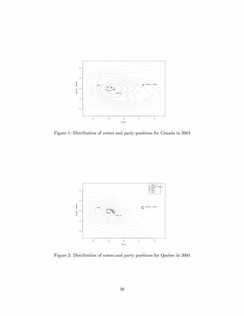
Social

Dec

entr

aliza

tion

­2 ­1 0 1 2

­2­1

01

2

Q

+

+++

+Conser v ativ e

NDPBQ

Liber al

Green

Figure 1: Distribution of voters and party positions for Canada in 2004

Social

Dec

entr

aliza

tion

­2 ­1 0 1 2

­2­1

01

2

Q

L

CNB

G

LCNGB

Liber alConser v ativ eNDPGreenBloc

Conser v ativ e

NDPBQ

Liber al

Green

Figure 2: Distribution of voters and party positions for Quebec in 2004

38

Social

Dec

entr

aliza

tion

­3 ­2 ­1 0 1 2 3

­2­1

01

2

++ + ++

NDPGPC

LPCBQ

CPC

Figure 3: Vote maximizing positions in Canada 2004

39

Spatial Model of Elections in Turkey: TracingChanges in the Party System in the 2000s

Norman Schofield and Betul Demirkaya

IntroductionDuring the first decade of the 21st century, electoral politics in Turkey

underwent significant changes in terms of both the number and the ideologicalpositions of political parties. The 1990s were marked by a historically highdegree of fragmentation with the effective number of parties rising to 4.3 in1995 elections and 4.8 in 1999 elections (Ozbudun 2000; Kalaycioglu 2008).This was partly due to a decrease in the vote share of the center-right andcenter-left parties and a concurrent rise in the vote share of the nationalistand Islamist parties. The 1999 elections resulted in a parliament with fiveparties, each with seat shares ranging between 15% and 25%. 1 A coalitiongovernment was formed by the center-left Democratic Left Party (DSP), thenationalist Nationalist Action Party (MHP) and the center-right MotherlandParty (ANAP). The 2001 financial crisis was followed by an early election in2002, in which none of the parties from the previous parliament were able to passthe electoral threshold. 2 The new parliament was formed by the members ofthe Justice and Development Party (AKP)– a new conservative party foundedby the former members of Islamist parties– and the Republican People’s Party(CHP)– a party with a strong emphasis on a secularist agenda. In the 2007elections, AKP consolidated their power by receiving 46.6% of the votes whileCHP increased their share of the vote by only 1.5 percentage points to 20.9%.In addition, the Nationalist Action Party (MHP) and independent candidatessupported by the pro-Kurdish Democratic Society Party (DTP) were able towin seats in the 2007 elections.

[Insert Tables 1 and 2 here]

The changes in electoral politics brought about several important ques-tions: What are the main issues that shape political debate? How can wedescribe the position of AKP and other parties on issues that are relevant forvoters? How can we explain the voters’preferences in this new electoral land-scape? The characterization of political parties and voters along a left-rightcontinuum has been widely-used and helpful in making comparisons across po-litical systems. However, the reduction of political views to a single dimension

1See Tables 1 and 2 for vote and seat shares of parties in the last four elections.2According to the electoral law of 1983, a political party needs to win at least 10% of the

national vote in order to win seats in the parliament.

1

may conceal the diversity of issues that may cut across each other. Moreover,the substantive content of the left-right continuum may change across countriesand over time. It has been discussed that economic and social issues that de-fine the political space in advanced industrial democracies were not suffi cient indescribing the electoral politics in Turkey in 2000s (Onis 2009). Self-placementof voters on a left-right continuum is explained by ethnic and sectarian differ-ences rather than socioeconomic characteristics (Carkoglu 2007). Religion andnationalism emerge as the primary dimensions that separate voters and politicalparties in the spatial analyses of 1999 and 2002 elections. AKP is located on theright on the religion axis albeit closer to the electoral mean than the Islamistparties while CHP is located on the left. On the nationalism axis, there is pro-Kurdish DTP on the one end and Turkish nationalist MHP on the other endwith other parties placed in between. (Hinich and Carkoglu 2006; Schofield etal. 2011). In this paper, we apply the spatial model described in the followingsection to the 2007 elections in order to trace the changes in the position ofvoters and parties.Spatial Model of ElectionsWe start our analysis with a pure spatial model M(λ, β) which includes

the distance between the position of the voters and the political parties andthe exogeneous valence (Schofield 2008). The valence term refers to the voters’perceptions of political leaders that are independent from their policy positions(Stokes 1963). In the model, the utility that voter i with position xi gets fromvoting for party j with position zj equals

uij(xi, zj) = λj − β‖xi − zj‖2 + εjIn the equation, ‖xi − zj‖ denotes the Euclidian distance between the voter

i’s ideal point and the party j’s policy position. εj is an error vector with a typeI extreme value distribution. The intercept term λj gives the exogeneous valenceof party j. The valence is exogeneous in the sense that it is not determined bythe characteristics of the voter. We use a multinomial logit model to estimatethe coeffi cients.

We continue our analysis with the calculation of convergence coeffi cientc which gives information about whether or not the position of the mean voterwould be an Local Nash Equilibrium (LNE) given the spatial coeffi cient andthe relative valence terms in the model. Schofield (2007) proves that c < 1 isa suffi cient and c < ω is a necessary condition for electoral mean to be a LNE,where ω is the number of dimensions. By simulation, we search for a LNE andsee whether the small parties have any incentive to diverge from the center giventhe spatial coeffi cient and the relative valence terms.

Finally, we incorporate the demographic charactersitcs of voters into thespatial model. In the joint model M(λ, β, θ), the utility of voter xi from votingfor party zj equals

uij(xi, zj) = λj + (θj · ηi)− β‖xi − zj‖2 + εj

2

where (θj · ηi) refers to the sociodemographic valence of voter i for party j(Schofield 2007).2007 Elections in TurkeyWe analyze 2007 elections based on World Values Survey (WVS) conducted

on a nationally representative sample in 2007.3 We limit our analysis to thevoters who indicated that they would vote for a political party in the followingelections and answered all the questions used in the factor analysis. 4 5 We usefactor analysis to identify the issues that differentiate voters from each other.We start with a long list of questions about the attitudes of voters towardreligion and nationalism as well as economic and social issues. 6 Similar toprevious studies, our analysis shows that religion and nationalism are principaldimensions that characterize the ideological position of Turkish voters. 7

[Insert Figure 1 here]

Figure 1 shows the position of voters with the x axis corresponding to thereligion dimension and the y axis corresponding to the nationalism dimension.A movement from left to right on the x axis indicates a view that favors anincreasing role of religion in private and public life. A movement from south tonorth on the y axis indicates an increasing association with Turkish nationalism.The variance on the x axis is 0.729 while the variance on the y axis is 0.498.The covariance between the two axes is 0.073. Thus the voter covariance matrixis the 2 X 2 matrix:

∇ =[0.729 0.0730.073 0.498

]with trace(∇)=1.227. The covariance matrix reveals two important points

that differ from the analysis of previous elections.8 First, the variance on thenationalism dimension is considerably smaller. The majority of voters are con-centrated on the northern part of the Figure 1 with higher levels of associationwith Turkish nationalism. There is another group of voters concentrated on thesouthern part of the figure , most of whom are the voters of the pro-KurdishDTP. Second, the covariance between the two axes is considerably smaller, which

3World Values Survey 1981-2008 Offi cial Aggregate v.20090901, 2009. World Values SurveyAssociation (www.worldvaluessurvey.org). Aggregate File Producer: ASEP/JDS, Madrid.

4Due to low levels of response to survey questions used to measure the position of voters,DTP voters are underrepresented in the sample compared to the election results, which mayhave a deflating influence on the valence term for DTP.

5We excluded the voters of Felicity Party, Young Party and Democratic Left Party fromour analysis. The vote shares for Felicity Party and Young Party were below 5% in the 2007elections (See Table 1). As explained in Table 1, after a failed attempt to merge with ANAP,DYP changed its name to DP in the 2007 elections. ANAP withdrew from the elections buttheir leader recommended that their voters vote for DYP. We decided to include these twoparties separately in our analysis because at the time survey was conducted and until theelections, they were two distinct parties with different voter profiles.

6The questions used in the factor analysis and the model are listed in Appendix 1.7The factor loadings of the analysis are given in Appendix 2.8See Carkoglu and Hinich 2006 and Schofield et al. 2011 for a spatial analysis of 1999 and

2002 elections in Turkey.

3

implies that the attitudes toward nationalism are not related very strongly tothe attitudes toward religion.

The position of parties is calculated by taking the mean position of its vot-ers on the religion and nationalism dimensions respectively. The party positionsare given by the following matrix:

z∗ =

Party AKP CHP MHP DTP DY P ANAPx : religion 0.31 −0.67 0.03 −0.1 0.04 −0.46

y : nationalism 0.07 −0.09 0.16 −1.4 0.22 −0.23

The position of parties is similar to the previous elections with relatively

minor differences. On the religion axis, CHP and AKP are located at theopposite ends with all the other parties located in between. Although position ofAKP on the religion dimension is closer to the center compared to the positionof pro-Islamist parties in previous elections, it is located to the right of theelectoral mean. On the nationalism axis, there is a polarization between thepro-Kurdish DTP on the one hand, and all the other parties on the other hand.As discussed above, the position of parties other than DTP are very close toeach other on this dimension. We are cautious, however, to interpret this asa change in the position of parties since we used questions that are differentfrom the previous analyses. Due to the lack of questions related to policies onissues such as language, we used questions that measure association with Turkishnationalism. Interestingly, and unlike the previous years, the nationalist MHPis closer to the center on this dimension than DYP; however, this may be relatedto the small number of DYP supporters both in the population in 2007 electionsand in our sample.

[Insert Table 3 here]

We use the pure spatial modelM(λ, β) to estimate the relationship betweenthe ideological position and valence of political parties, and their electoral suc-cess. The results are summarized in Table 3. The spatial coeffi cient β is 0.658and statistically significant. The valence terms are calculated with respect toMHP. The vector of relative valences is

(λAKP , λCHP , λMHP , λDTP , λDY P , λANAP ) = (1.413, 0.623, 0,−1.688,−1.479,−1.676)

The party with the lowest valence is DTP with λDTP = −1.688. Accordingto the model, when all parties are located at the electoral mean, the probabilitythat a voter chooses DTP is

4

ρDTP =exp(−1.688)

exp(1.413) + exp(0.623) + exp(0.0) + exp(−1.688) + exp(−1.479) + exp(−1.676)

= [exp(3.101) + exp(2.311) + exp(1.688) + exp(0) + exp(0.209) + exp(0.012))]−1

= [22.225 + 10.084 + 5.409 + 1 + 1.232 + 1.012]−1

= 0.024

The standard error for λDTP is 0.36. Accordingly, the 95% confidence in-terval for λDTP is [-2.398,-0.978] and the 95% confidence interval for ρDTP is[0.01,0.05]. As explained above, DTP did not participate in the 2007 electionsbut supported independent candidates; therefore, it is diffi cult to assess the voteshare of DTP in 2007. Table 1 shows that the independent candidates received5.24% of the votes; however, this includes candidates that were not supportedby DTP as well. The respondents that indicated that they would vote for DTPconstitue 2.5% of our sample.

Schofield (2007) defines a convergence coeffi cient,c, of the pure spatialmodel which is given by

c = 2β(1− 2ρDTP )trace(∇)= 2× 0.658× (1− 2× 0.024)× 1.227= 1.537

We calculate a conservative confidence interval for the convergence coeffi centusing the upper bound of the β coeffi cient and the lower bound of ρDTP andvice versa. The standard error for β is 0.061 so the 95% confidence interval is[0.538,0.778]. Thus, the 95% confidence interval for the convergence coeffi cientis [1.188,1.871]. The confidence interval for the convergence coeffi cient satisfiesthe necessary condition for the electoral mean to be an LNE since the upperbound is smaller than 2. It does not, however, satisfy the suffi cient conditionsince the lower bound is greater than 1.

The Hessian, or the characteristic matrix of DTP:

CDTP = 2β(1− 2ρDTP )∇− I= 2× 0.658× (1− 2× 0.024)∇− I

= 1.253

[0.729 0.0730.073 0.498

]− I

=

[−0.087 0.0910.091 −0.376

]

5

The eigenvalues of the characteristic matrix are -0.06 with the eigenvector(-0.961,-0.278) and -0.403 with the eigenvector (-0.278,0.961). We calculate aconfidence interval for the Hessian using the upper bound of the β coeffi cientand the lower bound of ρDTP and vice versa.

CDTP = 2β(1− 2ρDTP )∇− I= 2× 0.538× (1− 2× 0.05)∇− I, 2× 0.778× (1− 2× 0.01)∇− I

= 0.968

[0.729 0.0730.073 0.498

]− I, 1.525

[0.729 0.0730.073 0.498

]− I

=

[−0.294 0.0710.071 −0.518

],

[0.112 0.1110.111 −0.241

]The eigenvalues of the lower bound for the characteristic matrix are -0.273

with the eigenvector (-0.96, -0.279) and -0.539 with the eigenvector (-0.279,0.96).The eigenvalues of the upper bound for the characteristic matrix are 0.144 withthe eigenvector (-0.961, -0.277) and -0.273 with the eigenvector (-0.277, 0.961).

Schofield (2007) shows that a necessary and suffi cient condition for theelectoral mean to be LNE is that the eigenvalues of the characteristic matrixare negative. As we see above, the point estimate and the lower bound for thecharacteristic matrix have negative eigenvalues, which implies that the electoralmean should be LNE. The upper bound for the characteristic matrix has onepositive and one negative eigenvalue, and a negative determinant (0.15). Hence,the upper bound gives a saddle point.

By simulation based on the point estimates of the spatial coeffi cients andthe valence terms, we can verify that the electoral mean is an LNE in our case.When all the parties are located at the electoral mean their predicted vote shareswere calculated as:

ρz0 = (ρz0AKP , ρz0CHP , ρ

z0MHP , ρ

z0DTP , ρ

z0DY P , ρ

z0ANAP )

= (0.543, 0.246, 0.132, 0.024, 0.03, 0.025)

We compare this to votes shares in our sample9 :

(sAKP , sCHP , sMHP , sDTP , sDY P , sANAP )

= (0.556, 0.231, 0.134, 0.025, 0.03, 0.023)

9We cannot directly compare the actual and the sample vote shares because of the changein the list of parties that participated in the elections. The vote shares of AKP, CHP andMHP in 2007 elections were 46.58%, 20.88% and 14.27%, respectively. DTP did not enter theelections but supported independent candidates. DYP changed its name to DP and received5.42% of the votes. ANAP did not enter the elections but their leader asked their supportersto vote for DP. One should also note that our analysis excludes the voters of small partieswhich account for 8.63% of the votes in 2007 elections. See Table 1 for the vote shares.

6

This comparison is important as it tells us about whether the low valenceparties have any incentive to move to the electoral mean. Schofield and Gallego(2011, 190) call an equilibrium at position z a stable attractor when the lower95% bound of predicted vote shares of low valence parties at the equilibrium arehigher than their actual vote shares. If an equilibrium is not a stable attractorthan the party activists would have more incentive to pull the party from theelectoral mean to z∗. As we see in the vectors, the equilibrium at the electoralmean is not a stable attractor for DTP or DYP.

By using simulation, we found another LNE with the following partypositions:

z1 =

Party AKP CHP MHP DTP DY P ANAPx : religion 0.02 0.05 0.08 −1.24 0.12 0.12

y : nationalism 0.02 0.04 0.05 −0.7 0.05 0.05

As can be seen in Figure 2, all the parties other than DTP are concentratred

around the electoral mean and DTP is on the southwest of the graph. Thedifference between the initial party positions and the party positions at theequilibrium is given by the following matrix:

z∗ − z1 =

Party AKP CHP MHP DTP DY P ANAPx : religion 0.29 −0.72 −0.05 1.14 −0.08 −0.58

y : nationalism 0.05 −0.13 0.11 −0.7 0.17 −0.29

This matrix shows how much and in which direction the parties are pulled

from the equilibrum point by the party activists. The most obvious differencesare seen in the positions of CHP and DTP. The former takes a position far tothe left of the equilibrium position on the religion axis and the latter takes aposition far to the south of the equilibrum poisiton on the nationalism axis. Thepredicted vote shares at the equilibrium were calculated as:

ρz1 = (ρz1AKP , ρz1CHP , ρ

z1MHP , ρ

z1DTP , ρ

z1DY P , ρ

z1ANAP )

= (0.539, 0.245, 0.131, 0.03, 0.03, 0.025)

Compared to the sample vote shares the equilibrum provides a higher pre-dicted vote share for CHP, DTP and ANAP.

[Insert Figure 2 here]

Finally, we supplement the spatial model with the demographic character-istics of voters. Following previous studies, we include age, education, ethnicityand socio-economic status as independent variables. We measure ethnicity bythe primary language that the respondents speak at home and construct it as adummy variable that takes the value 1 for Zaza and Kurdish, and 0 for Turkish

7

and all other languages. 10 Previous studies point to a relationship betweenreligious sect and vote choice. More specifically, Alevi voters were more likelyto vote for CHP compared to other parties (Schofield et al. 2011). We were notable to include religious sect in our analysis because the question was not askedto the respondents.

[Insert Table 4 here]

In the joint model, which is summarized in Table 4, the spatial coeffi cientis smaller than the pure spatial model but it is still statistically significant.However, none of the valence terms except the one for DTP are statisticallysignificant. Among the demographic characteristics, the only one that is bothsubstantively and statistically significant is ethnicity. Not surprisingly, Kurdishspeakers are more likely to vote for DTP compared to the baseline, which is thenationalist MHP. If we compare the Mc Fadden R2 of the pure model to thejoint model, we see that the joint model provides a better fit.Comparison with Previous ElectionsA comparison of our results with previous analyses of 1999 and 2002

elections enables us to trace the change in electoral politics in Turkey duringthe last decade. In order to facilitate comparison, we rerun the model by usingDYP as the baseline and summarized the results in Table 5. 11 The considerableincrease in the relative valence of the three parties in the parliament compared toDYP points to the culmination of the decline of center-right parties. The valenceof AKP increased compared to both CHP and MHP. This can be explainedby the good performance of AKP’s economic policies. 12 It is important tonote, however, that it is practical rather than ideological considerations abouteconomic policy that effect voters’ preferences. Our factor analysis did notdetect any coherent attitudes toward economic policy that explain the varianceamong voters. Economic policy can be thought as part of the valence term tothe extent it is perceived as the competence of the party leaders. The positivevalence terms for all three parties —AKP, CHP and MHP—can also partly beexplained by the role party activists in providing financial and organizationalresources.

[Insert Table 5 here]

One of the critical findings of our comparison is the decrease in the con-vergence coeffi cient from 5.9 in 2002 to 1.5 in 2007, which implies an increasinglikelihood of convergence to the electoral mean. By using simulation, we veri-fied that electoral mean gives an LNE in 2007 elections. We also found anotherLNE with all parties except DTP aligned close to the electoral mean and DTPlocated in the southwest of the ideological space. We argue that the electoral

10See Appendix 2 for the list of questions used to measure demographic characterisitcs.11 In the previous section, we use MHP as the baseline because the small number of DYP

supporters in our sample result in large standard errors in the joint model.12 In an analysis of 2007 elections, Kalaycioglu (2010) points that economic satisfaction is

the primary determinant of both party identification and party preference for AKP voters.

8

strength of AKP pulls the equilibrium point to the right of electoral mean onthe religion axis. The initial position of all parties except DTP and AKP areto the left of the equilibrium. The initial positions of parties except DTP onthe nationalism axis got closer to each other compared to 2002 elections. DTPtakes a position that is to the south of the equilibrium point.None of the partiesexcept DTP diverge from the electoral mean on this axis in the equilibrium.

9

BibliographyCarkoglu, Ali and Melvin J. Hinich. 2006. “A Spatial Analysis of Turkish

Party Preferences." Electoral Studies 25(2):369-392.Carkoglu, Ali. 2007. “The Nature of Left-Right Ideological Self-placement

in the Turkish Context." Turkish Studies 8(2): 253-271.Kalaycioglu, Ersin. 2008. “Attitudinal Orientation to Party Organizations

in Turkey in the 2000s." Turkish Studies 9(2):297-316.Kalaycioglu, Ersin. 2010. “Justice and Development Party at the Helm:

Resurgence of Islam or Restitution of the Right-of-Center Predominant Party?"Turkish Studies 11(1):29-44.Onis, Ziya. 2009. “Conservative Globalism at the Crossroads: The Justice

and Development Party and the Throny Path to Democratic Consolidation inTurkey" Mediterranean Politics 14(1):21-40.

Ozbudun, Ergun. 2000. Contemporary Turkish Politics: Challenges to De-mocratic Consolidation. Boulder, Colo: Lynne Rienner Publishers.Schofield Norman. 2007. “The Mean Voter Theorem: Necessary and Suf-

ficient Conditions for Convergent Equilibrium." Review of Economic Studies74(3):965-980.Schofield, Norman. 2008. The Spatial Model of Politics. New York: Rout-

ledge.Schofield, Norman and Maria Gallego. 2011. Leadership or Chaos: The

Heart and Soul of Politics. Berlin; New York: Springer.Schofield Norman, Maria Gallego, Ugur Ozdemir and Alexei Zakharov. 2011.

“Competition for Popular Support: A Valence Model of Elections in Turkey."Social Choice and Welfare 36(3):451-482.Stokes, Donald E. 1963. “Spatial Models of Party Competition." American

Political Science Review 57(2):368-377.World Values Survey 1981-2008 Offi cial Aggregate v.20090901, 2009. World

Values Survey Association (www.worldvaluessurvey.org). Aggregate File Pro-ducer: ASEP/JDS, Madrid.Appendix 1 Survey QuestionsThe analysis of 2007 elections in this paper is based on World Values Survey

(WVS).13The survey was conducted between January and March 2007, that isthree - six months before the 2007 elections. The questions used in our analysisare the following:Vote ChoiceIf there were a national election tomorrow, for which party on this list would

you vote?Secularism1) How strongly do you agree or disagree with each of the following state-

ments? Strongly Agree, Agree, Neither Agree Nor Disagree, Disagree, StronglyDisagreea)Politicians who do not believe in God are unfit for public offi ce.

13World Values Survey 1981-2008 Offi cial Aggregate v.20090901, 2009. World Values SurveyAssociation (www.worldvaluessurvey.org). Aggregate File Producer: ASEP/JDS, Madrid.

10

b)It would be better for Turkey if more people with strong religious beliefsheld public offi ce.2) For each of the following, indicate how important it is in your life. Would

you say it is Very important Rather important Not very important Not at allimportant? ReligionNationalism1) How proud are you to be Turkish? Very Proud, Quite Proud, Not Very

Proud, Not At All Proud2) People have different views about themselves and how they relate to the

world. Using this card, would you tell me how strongly you agree or disagreewith each of the following statements about how you see yourself? I see myself aspart of the Turkish nation. Strongly Agree, Agree, Disagree, Strongly DisagreeDemographic Characteristics1) Age: Can you tell me your year of birth, please? This means you are ...

years old.2) Education: What is the highest educational level that you have attained?

1-No Formal Education 9-University Level Education - With Degree3) Language: What language do you normally speak at home?4) Socio-economic Status: People sometimes describe themselves as belong-

ing to the working class, the middle class, or the upper or lower class. Wouldyou describe yourself as belonging to the 1 Upper class 2 Upper middle class 3Lower middle class 4 Working class 5 Lower class?Appendix 2 - Factor Loadings

Factor Loadingsn=588 Religion NationalismPoliticians’belief in god 0.738 0.092People with strong beliefs in public offi ce 0.748 0.064Religion important in life 0.478 0.246Proud of nationality 0.071 0.656Part of the nation 0.106 0.405Variance 0.270 0.133Cumulative Variance 0.270 0.403

11

TablesTable 1 - Vote Shares (%) - 1999 - 2011

Vote SharesParty Name 1999 2002 2007 2011Justice and Development Party AKP - 34.28 46.58 49.80Republican People’s Party CHP 8.71 19.39 20.88 25.98Nationalist Action Party MHP 17.98 8.36 14.27 13.02Felicity Party SP a - 2.49 2.34 1.26Virtue Party FP 15.41 - - -Democrat Party DP - 5.42 b 0.65Democratic Left Party DSP 22.19 1.22 - c 0.25True Path Party DYP 12.01 9.54 - 0.15Motherland Party ANAP 13.22 5.13 - d -Genc Party GP - 7.25 3.04 -People’s Democracy Party HADEP 4.75 - -Democratic People Party DEHAPe - 6.22 - -Independents 0.87 1.00 5.24 f 6.59 f

Others 4.86 5.13 2.25 2.29Total 100.00 100.00 100.00 100.00Turnout 87.09 79.14 84.25 83.16

Notes: a) Felicity Party is the successor to Virtue Party, which was bannedby the Constitutional Court. b) DYP changed its name to Democrat Party ina failed attempt to merge with ANAP. c) The candidates of DSP entered theelections in the CHP lists. d)ANAP did not enter elections and their leader askedtheir supporters to vote for DP. e) Democratic People Party is the successorto People’s Democracy Party, which was banned by the Constitutional Court.f) Majority of independent candidates are supported by Democratic SocietyParty(DTP), which is the successor to DEHAP.Source: www.ysk.gov.tr; www.resmigazete.gov.tr

12

Table 2 - Seats - 1999 - 2011

SeatsParty Name 1999 2002 2007 2011Justice and Development Party AKP - 363 (66) 341 (59.56) 327 (59.45)Republican People’s Party CHP - 178 (32.36) 112 (20.4) 135 (24.55)Nationalist Action Party MHP 129 (23.45) - 70 (12.75) 53 (9.64)Felicity Party SP - - - -Virtue Party FP 111 (20.18) - - -Democrat Party DP - - - -Democratic Left Party DSP 136 (24.73) - - -True Path Party DYP 85 (15.45) - - -Motherland Party ANAP 86 (15.64) - - -People’s Democracy Party HADEP - - - -Independents 3 (0.55) 9 (1.64) 26 (4.74) 35 (6.36)Others - -Total 550 (100.00) 550 (100.00) 549 (100.00) 550 (100.00)

Source: www.ysk.gov.tr; www.resmigazete.gov.tr

Table 3 - Pure Spatial Model for 2007 Elections

Pure Spatial Model for 2007 ElectionsNormalized with respect to MHPParty Name λ Std. error |t-value|Justice and Development Party AKP 1.413∗ 0.129 10.93Republican People’s Party CHP 0.623∗ 0.151 4.138Nationalist Action Party MHP - - -Democratic Society Party DTP −1.688∗ 0.36 -4.684True Path Party DYP −1.479∗ 0.269 -5.507Motherland Party ANAP −1.676∗ 0.302 -5.551Spatial Coeffi cient β 0.658∗ 0.061 -10.758Convergence Coeffi cient 1.537n=558; Log likelihood = -603.57; McFadden R2 = 0.114* Significant with probability < 0.001

13

Table 4 - Joint Model for 2007 Elections

Joint Model for 2007 ElectionsNormalized with respect to MHPVariable Party Coeffi cient Std. error |t-value|Spatial Coeffi cient β 0.603∗∗∗ 0.066 −9.167Relative Valence λk AKP −0.694 1.228 −0.565

CHP −1.171 1.625 −0.72DTP −5.183∗ 2.229 −2.326DYP 11.571 3083.355 0.004ANAP 11.583 4329.811 0.003

Age AKP 0.025∗ 0.012 2.205CHP 0.032∗ 0.013 2.411DTP 0.004 0.032 0.109DYP 0.063∗∗ 0.019 3.266ANAP 0.025 0.025 0.995

Education AKP −0.227∗ 0.095 −2.392CHP 0.118 0.107 1.104DTP −0.285 0.288 −0.988DYP −0.228 0.193 −1.181ANAP −0.113 0.209 −0.542

Kurdish AKP 1.486 1.045 1.423CHP −0.359 1.441 −0.249DTP 4.653∗∗∗ 1.245 3.738DYP −14.527 3083.354 −0.005ANAP −14.965 4329.811 −0.003

Socio-economic Status AKP 0.314∗ 0.145 2.164CHP 0.288 0.174 1.651DTP −0.36 0.484 −0.744DYP 0.252 0.305 0.826ANAP 0.541 0.36 1.503

n=558; Log likelihood = -565.6; McFadden R2 = 0.17*** Significant with probability < 0.001** Significant with probability < 0.01* Significant with probability < 0.05

14

Table 5 - Comparison with Previous Years

Comparison with Previous YearsNormalized with Respect to DYPParty Name 1999 2002 2007Justice and Development Party - 0.78∗ 2.893∗

Republican People’s Party 0.734∗ 1.33∗ 2.102∗

Nationalist Action Party 0.666∗ -0.12 1.479∗

Democratic Society Party -0.071 0.43 −0.209Motherland Party 0.336 -0.31 −0.197Democratic Left Party 0.724∗ - -Spatial Coeffi cient β 0.375∗ 1.52∗ 0.659∗

Convergence Coeffi cient 1.49∗ 5.94∗ 1.54∗

Source: The entries for 1999 and 2002 are the results of the analysis inSchofield et al. 2011.

Figures

15

­1.0 ­0.5 0.0 0.5 1.0­1.5

­1.0

­0.5

0.0

0.5

Religion

Nat

iona

lism

AKPCHP MHP

DTP

D YP

ANAP

Figure 1: Voter Distribution and Party Positions in 2007 Elections

16

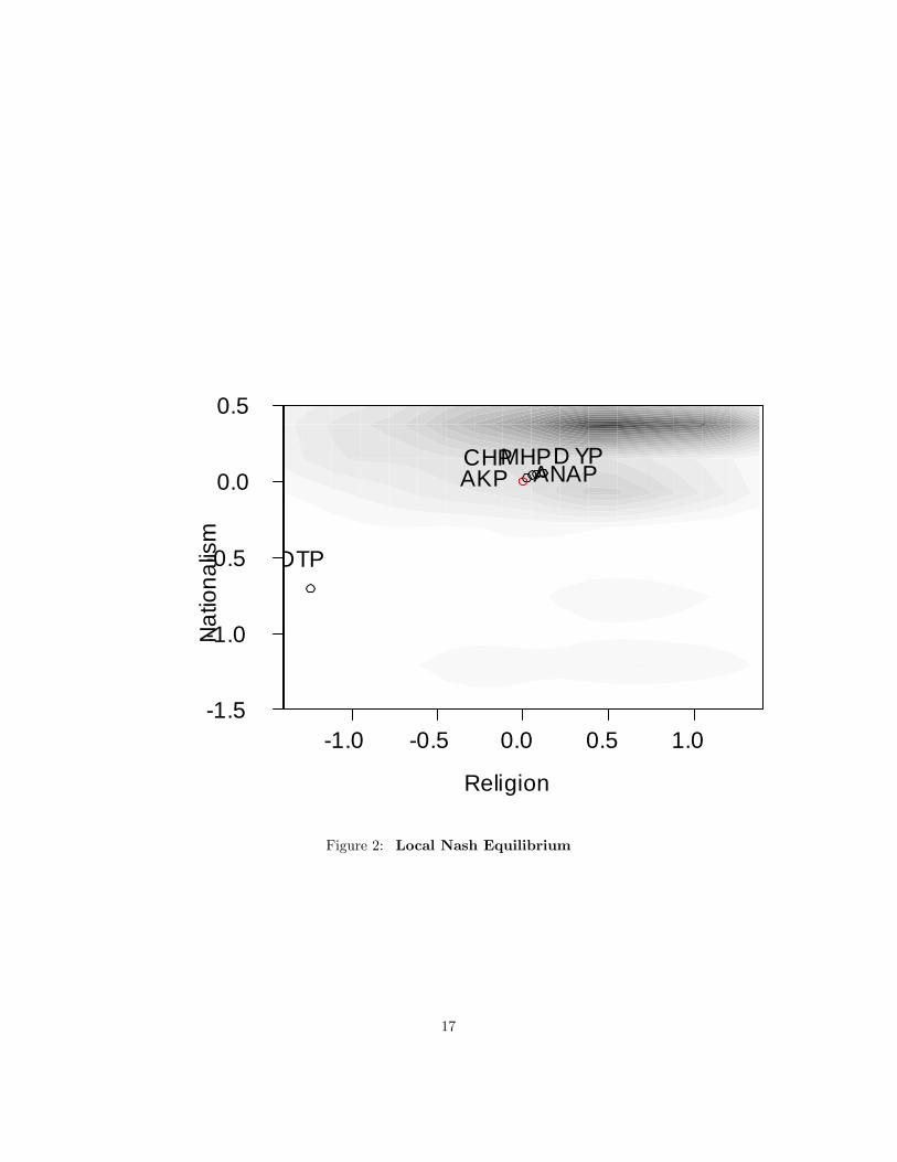
­1.0 ­0.5 0.0 0.5 1.0­1.5

­1.0

­0.5

0.0

0.5

Religion

Nat

iona

lism

AKPCHPMHP

DTP

D YPANAP

Figure 2: Local Nash Equilibrium

17

Do Competitive Districts Necessarily Produce Centrist Politicians?

James Adams Department of Political Science University of California, Davis

Thomas L. Brunell

School of Economic, Political and Policy Sciences The University of Texas at Dallas

Bernard Grofman

Department of Political Science and

Center for the Study of Democracy University of California, Irvine

Samuel Merrill, III

Department of Mathematics and Computer Science Wilkes University

May 1, 2012

*We are indebted to Keith Poole for making available to us Poole-Rosenthal DW-NOMINATE data for the House for the period of interest, and to Dan Butler for helpful comments on a previous version of the manuscript. We also owe special thanks to Clark Bensen of POLIDATA who routinely provides us with high quality aggregate election data. We are indebted to Clover Behrend-Gethard and Sue Ludeman for bibliographic assistance. The listing of authors is alphabetical. Work on this project by the third-named author was supported by SSHRCC research grant #410-2007-2153 (co-PIs Stanley Winer and J. Stephen Ferris) and by the Jack W. Peltason (Bren Foundation) Chair, University of California, Irvine.

1

I . Evaluating Conventional Wisdom about the Effects of District Composition on Party Convergence Among the Members of the U.S. Congress

We have come a long way from the simplistic portrait of two-party plurality

competition resulting in tweeedledum-tweedledee politics that is commonly attributed to

Downs (1957).1 Two key modifications are the recognition that (1) paralleling Downsian

pressures for party convergence, there are strong competing incentives for party

divergence; and, (2) that the existence of multiple legislative constituencies in which

competition occurs affects the standard Downsian logic.

For example, we now recognize the theoretical potential for divergence due to

politicians’ sincere policy motivations,2 candidate nomination rules,3 party activists,

voters’ partisan loyalties, the threat of abstention due to alienation, and a host of other

factors.4 Theoretical research also suggests that the consequences of multi-constituency

competition for party convergence are expected to be larger (a) the more diverse the

locations of the median voter across different districts, (b) the greater the extent to which

candidates/elected officials have the leeway to modify their policy platforms/legislative

behavior to accommodate the median voter in their own district,5 and (c) the greater the

difference in variance in the support bases of the two parties.6 Neo-Downsian models of

the type pioneered by Adams and Merrill (2003), Butler (2009), and Miller and Schofield

(2003) demonstrate that, under certain empirically plausible circumstances, candidates

maximize support in general elections not by appeal to the median voter position but by

mobilizing their own partisan supporters (i.e., what we think of as the party’s “base”).

There is also extensive empirical support for party divergence in two party

competition in the United States, including work on the ideological differences between

Senators of the same state from rival parties (e.g., Poole and Rosenthal, 1984; Grofman,

Griffin, and Glazer, 1990), work that tests hypotheses about the extent to which primary

voting rules affects party divergence (Gerber and Morton, 1998; Brunell and Grofman,

2001), and a body of work dating back as least as far as Froman (1963) looking at the

degree to which newly elected members of congress resemble their predecessors in

voting behavior and at the degree to which members of Congress are responsive to the

ideology of their constituents. For example, Schmidt, Kenny, and Morton (1996) test the

2

hypothesis that candidates derive electoral benefits in general elections from appealing on

policy grounds to their partisan constituencies. In a study of U.S. Senate elections from

1962-1990, they conclude that incumbent Senators were more likely to win reelection

when their voting records coincided with their state party’s platform than when their

voting records reflected the median state voter’s position, and, furthermore, that senators

who appealed to their state party constituencies were more likely to run for reelection.7

Griffin (2006) argues that district competitiveness promotes responsiveness.

Griffin’s analysis, however, does not address our main question of how the policy

differential between Democratic and Republican office-holders in similar districts varies

between competitive districts on the one hand and uncompetitive ones on the

other. What Griffin shows, instead, is that the average ideology of representatives (rather

than the differential between parties) varies across districts as the median voter ideology

varies, and that this relation is more pronounced among generally moderate districts than

among uncompetitive districts.8 Griffin, however, does not compare Democratic

positions with Republican positions in similar districts.

In this essay we show that theoretically expected patterns of candidate positioning

are reflected in the empirical record of the ideological locations of those individuals who

become members of Congress. In particular, we look at the implications of presidential

voting patterns at the district/state level – which we view as a surrogate for district/state

ideology – for the degree of ideological similarity among Democratic and Republican

officeholders, as reflected in their legislative voting records. We analyze data for the

U.S. House and Senate over the period 1956-2004. We take support levels for

Democratic presidential nominees as our measure of the underlying ideological

predisposition in the district, and we use the first dimension of DW-NOMINATE scores

as our measure of the policy positions taken by officeholders. Our focus is empirical and

descriptive rather than theoretical (although, as we discuss below, our findings have

important implications for theory-based models of candidate competition).9

Exactly as expected, we find that representatives from opposite parties who are

elected from districts of similar ideology display sharply different legislative voting

records, such that, for any given level of Democratic presidential support, Democrats

elected from such districts are, on average, considerably more liberal than Republicans

3

elected from such districts. Moreover, we also find the expected constituency-specific

effects that pull office holders toward the views of their own constituency, so that the

greater the support for Democratic presidential nominees in the district, the more liberal

are both Democratic and Republican officeholders from such districts.

We look more closely at the degree of ideological similarity among officeholders

of the two parties as a function of presidential voting in the district. We also consider

differences found across different time periods and offer evidence from both Houses of

Congress. In particular, rather than looking at each party separately, we look at whether

the degree of closeness/competiveness in the underlying partisan characteristics of a

district lead to differences in the ideological gap between representatives of the two

different parties elected from districts of that type.

Our primary purpose is to investigate the theoretical expectations derived from

the modeling of Adams, Merrill and Grofman (2005), Butler (2009), and Adams et al.

(2010), that policy convergence between vote-seeking Democratic and Republican

candidates need not be maximized in districts with balanced partisan compositions, i.e.,

where there are approximately equal proportions of Democratic and Republican

partisans. Indeed, Adams et al. (2010), who account for voters’ partisan loyalties and

abstention due to alienation, advance the opposite argument, that, ceteris paribus,

districts with balanced partisan compositions will motivate maximal policy divergence

between Democratic and Republican candidates. Figure 1 in Adams et al. (2010) depicts

the expected pattern, i.e., ideological divergence is greatest when partisans are equally

balanced. Although the arguments of Adams et al. and Butler10 apply to the degree of

policy divergence between rival candidates (one of whom must lose), while our analyses

consider only winning candidates, these authors’ arguments imply that when comparing

the ideological positions of winning candidates from different parties, these differences

should be at least as large in competitive districts as in non-competitive districts.

We focus on winners because we recognize that idiosyncratic factors may drive

the locations of the candidate of the minority party in uncompetitive seats, and our

interest is about how different from the location of the median voter a candidate can be

and still be able to win the district. We treat idiosyncratic candidate characteristics and

incumbency advantages as effectively washing out when we compare the set of

4

Democratic and Republican winners from districts with the same ideological

characteristics (as inferred from presidential election outcomes). Under these

assumptions, we evaluate the hypothesis that the difference in policy positioning between

Democratic and Republican winners should be at least as large in districts where the

presidential outcome is competitive as in districts where the presidential outcome is non-

competitive.

In the recent theoretical models, unlike the standard Downsian model, being in a

potentially competitive seat does not necessarily imply that winners are closer to the

median voter in the district. This is because, in such competitive settings, candidates

have various strategic options to seek to improve their election chances, such as gaining

financial support from an activist and interest-group base and using the money and

publicity it buys to appeal to less ideologically-oriented voters (see e.g., Schofield and

Miller, 2007). Such an appeal can result from emphasizing one’s own competence or

likeability, by attacking the opponent, or by appealing to one’s own party base and trying

to further mobilize it. When candidates in a potentially competitive district seek support

from potential activists – who are typically more polarized than the general electorate –

they move further away from the median voter in that district. Candidates can

compensate for being more distant from the median voter than their opponent by

increasing turnout and activism11 among their own party faithful.

To gain intuition about why candidates might be most dispersed when the election

is most competitive, Adams et al. (2010) first consider the least competitive election

context, namely that in which all citizens in the electorate identify with the same party.

If, say, all citizens are Democratic partisans, then both candidates will appeal on policy

grounds to these partisans, since there are no others. Therefore -- even while courting

citizens to vote and activists to contribute -- margin-maximizing candidates will converge

to identical positions in this “perfectly” uncompetitive scenario, and, by extension, they

can be expected to converge to similar positions for partisan contexts that strongly favor

one party over the other.

By contrast, in competitive districts, each candidate is motivated to appeal in large

part to his/her own partisan constituency, which motivates increased divergence of the

candidates’ positions. To see intuitively why this might be true, Adams et al. (2010)

5

consider another extreme situation where voters’ partisan biases are so strong that they

invariably prefer their party’s candidate to the rival party’s candidate, regardless of the

candidates’ positions, but where partisan voters are also prone to abstain from voting

and/or activism, so that they participate only if they approve of their preferred candidate’s

policy position. Because, in this scenario, each candidate influences decisions to

participate by the members of only her own partisan constituency – and neither candidate

can attract support from the rival party’s partisans – each candidate is motivated to give

weight to the policy preferences of her own partisan constituency (along with the

preferences of any independent voters in the electorate), while ignoring the policy

preferences of the rival party’s partisan constituency.12

Our empirical analyses support this expectation that candidates may be most

dispersed when the election is most competitive. We find that, contrary to the intuition

that competitive districts should pull candidates of opposite parties closer together toward

the median voter in that district, the ideological difference between the winners from the

two parties is typically as great or greater in districts that, in presidential support terms,

are the most competitive. Simply put, in election contexts that one might think give

candidates the strongest possible incentives to maximize their electoral support, the

winning candidates tend to present the most radical policies relative to the center of

district opinion. Note that this finding does not imply that the most competitive districts

elect the most extremist members of Congress. Rather it indicates that Democrats and

Republicans elected in competitive districts are at least as polarized relative to each other

– but not necessarily more extreme -- than those elected in lopsided districts.

We believe empirical research on the policy extremism of candidates contesting

competitive districts is relevant not only to the theoretical models of Butler (2009) and

Adams, Merrill, and Grofman (2005) discussed above, but also to the more general

question: Do candidates believe they maximize their support by converging towards the

center of district opinion, or by presenting noncentrist positions that may be more

appealing to their base and also to special interest groups?

As we noted above the basic Downsian model provides a strong intuition that, all

other factors being equal, candidates and parties enhance their support by moving to the

center of constituency opinion. However subsequent theoretical and empirical research

6

has developed several reasons why other factors are not equal, and may reward

candidates for presenting noncentrist positions. These include motivating turnout among

party supporters who hold noncentrist viewpoints; energizing party activists to work on

the candidate’s campaign13; motivating special interest groups to finance the campaign14;

and, convincing voters that the candidate is of superior character because her announced

noncentrist positions demonstrate that she is not “pandering” to voters in the district.15

Given these theoretical considerations it is not obvious whether, in real-world elections,

candidates enhance their electoral prospects by positioning themselves near the center of

the district electorate, or by presenting noncentrist positions that appeal to their partisans,

to party activists, and to special interest groups. The empirical findings we present below

that the winning candidates in more competitive districts present more radical policies

suggest that the candidates themselves believe there are electoral advantages to

noncentrist positioning. We believe this finding is important.

Our analysis is also consistent with the empirical findings of Ansolabehere,

Snyder and Stewart (2001), who find little support for the claim that winners of

competitive races are more ideologically centrist than members of that same party elected

from safe seats. Ansolabehere, Snyder and Stewart (2001) look at the degree of

divergence between winners and losers.

Unlike these and most other authors, we define competition in a national (i.e.,

presidential) rather than a House/Senate contest-specific way. Here, because DW-

NOMINATE scores are generally available for winners but not for losers, we look only at

the positions of winners. But, of course, it is the winners who matter most. There are

advantages and disadvantages to both approaches – i.e., defining competition in a

national or a contest-specific way – and they should be seen as complementary. When

Ansolabehere, Snyder, and Stewart (2001) and others define competition in terms of

contests for House seats, they look directly at the competitiveness of the election in

which a given officeholder is elected. On the other hand, any given House contest

involves idiosyncratic features such as the backgrounds and campaign skills of the two

candidates (and controlling for incumbency only partly controls for these other effects).

This problem is exacerbated by the fact that there are only a few data sets that contain the

ideological locations of both challengers and candidates. In contrast, by using

7

presidential level data for all districts we provide more comparable data on the

underlying partisan predispositions of the districts and we have comparable data over a

larger number of districts over a much longer time period. In addition, potential

statistical problems arise if we substitute votes in the House/Senate elections themselves

for the presidential vote shares. Specifically, if we regress DW-NOMINATE scores on

vote shares in House/Senate elections, this regression introduces an endogeneity problem

because the Democratic proportion of the vote in each election is in part dependent on the

ideological positions of the Congressional candidates, which biases estimates of the

regression parameters.16 Thus, there are good reasons to believe that the kind of data

which we analyze in this paper is informative about pressures for ideological divergence.

II. Ideological Extremism in the U.S. House, 1956-2004, by Party and by Democratic Presidential Vote in the District

We begin by analyzing the relationship between candidate extremism and district

competitiveness, using data for U.S. House districts over the 1956-2004 period. Taking

DW-NOMINATE scores as our measure of a member’s ideology for data pooled for the

House elections from 1956 through 2004,17 we have plotted member DW-NOMINATE

scores against the (district-specific) normalized Democratic vote share in the district in

the contemporaneous Presidential election,18 which we use as an estimate of district

ideology. We label this variable the normalized district Democratic vote proportion for

president, or district ideology for short.

Plots for pooled data over the period 1956-2004 are presented in Figure 1; plots

broken down by time period are shown in Figure 2. Areas of the figure to the left of the

vertical line represent Republican districts, i.e., those in which the district Democratic

presidential vote was less than the national Democratic vote, while the areas to the right

of it represent Democratic districts. Each curve, one for each party, represents a

quadratic regression for that party, in which we regressed the representatives’ DW-

NOMINATE scores on the normalized district Democratic vote proportion, which we

take as a measure of district ideology, and on the square of the district ideology; we also

included a dummy variable for districts from the South.19 Thus for each party our

specification was:

8

DW-NOMINATE scorej = b1 + b2[District ideologyj]

+ b3[District ideologyj]2 + b4[South] , (1)

where

DW-NOMINATE scorej = representative j’s DW-NOMINATE score, based on j’s

legislative voting record in the two years preceding the

election.

District ideologyj = normalized presidential vote in j’s district, as defined in footnote 18.

[District ideologyj]2 = the square of the normalized presidential vote in j’s district.

South = 1 if the district was located in the South, and zero otherwise.

Inclusion of the term [District ideologyj]

2 in equation 1 allows us to investigate the

possibility of nonlinear effects of district ideology on the House member’s DW-

NOMINATE score, and to estimate how the degree of ideological dispersion between

Republican and Democratic representatives varies with district competitiveness.20 Table

1 reports these regression coefficients for the U.S. House, and the shaded regions in the

figures represent the 95 percent confidence regions for the regressions.21 As expected,

the parameter estimates reported in Table 1 and illustrated in Figures 1-2 support the

expectation that representatives’ ideological positions respond to the position of the

median voter by district, so that the fitted curve for each party slopes downward (party

responsiveness), both for the 1956-2004 period as a whole (Figure 1) and for each of the

time periods 1956-64, 1966-74, 1976-84, 1986-94, and 1996-2004 (Figure 2). All of

these downward slopes – for the full period (as well as for each subperiod) and for each

party – are statistically significant at the 0.001 level. In addition, note that the downward

slopes of these regression lines for both Democrats and Republicans are substantial,

suggesting mean within-party ideology does vary substantially as a function of the

presidential voting patterns in the district. For the analyses pooled over the entire 1956-

9

2004 time period, the estimated parameters on the linear coefficient reported in Table 1

are -0.75 for Democratic representatives and -1.03 for Republican representatives,

indicating a downward trend in the DW-NOMINATE score of about one tenth of a unit

for each increase of ten percent in the Democratic proportion of the district vote.22

On the other hand, if we look at the gap between the two curves, which reflects

differences across party lines, we find very substantial differences between the winners

from the two parties; for instance the pooled data in Figure 1 suggests that, on average, a

Republican Congressperson from even a 70 percent Democratic district can be expected

to be more conservative than a Democratic member from a 30 percent Democratic

district. The difference in regression intercepts between Democrats and Republicans

indicates the typical difference between the DW-NOMINATE scores of House members

of the two major parties when the partisan composition of the district is 50-50. As

reported in Table 1, these differences range from 0.52-0.57 DW-NOMINATE units in

each of the first three subperiods to 0.72 units in the most recent subperiod 1996-2004,

reflecting the increased polarization in the House.23 Clearly, party has a huge effect

relative to that of district ideology.24 Finally, the positive coefficient estimates on the

South dummy variable suggest that – particularly in the earlier time periods –

representatives tended to compile more conservative legislative voting records when they

were elected from Southern districts, compared to when they were elected from non-

Southern districts with similar presidential voting patterns.

So far we have considered what our data implies about House members’

responsiveness to district ideology, along with the ideological differences between

Democratic and Republican representatives. However our most interesting findings

concern how district ideology is related to partisan divergence, i.e., the degree of

ideological divergence between House members from different parties. As noted above,

the conventional wisdom is that partisan divergence will be greatest when the election is

not competitive, because in a lopsided district the candidate from the dominant party can

move away from either the national or district median and expect to win anyway. Given

that districts with highly unequal partisanship are likely to be less competitive in terms of

presidential voting, this conventional wisdom implies that we should observe the largest

10

ideological gap between Republican and Democratic representatives in districts that

feature lopsided presidential vote margins.

However the curves in Figure 1, which are fitted to the full 1956-2004 data, do

not conform to this pattern: instead they bow out slightly away from each other in the

middle of the partisan distribution scale.25 Note that neither for the full period (1956-

2004) nor for any of the five breakdown periods is there evidence that the curve for either

party is significantly bowed inward at the 0.05 level. By contrast, positive coefficients on

the quadratic term for the Democrats and negative coefficients for the Republicans

indicate significant outward bowing for both parties for the overall period and for the

earliest (1956-1964) and the latest (1996-2004) periods, each at the 0.05 level or better

(see Table 1 and Figure 2).26 In other words, Republican and Democratic House winners

are as different or more so in ideology in the most competitive districts than in un-

competitive ones. The outward bowing of the curves is not pronounced; what is

remarkable is that the curves do not bow inward, as we would expect if the partisan gap

narrowed in competitive districts.

Related plots are obtained by Erikson and Wright (2000). In particular, using the

NES seven-point scale for both axes, these authors plot the mean perception of the

ideology of incumbent House members during the 1980s against constituency ideology,

obtaining as we do a sharp separation between Democrats and Republicans and trends

reflecting party responsiveness (Erikson and Wright, 2000: Fig. 8.6). The authors’ scatter

plots for each party appear to show curvature that bows out between the parties, but this

possible effect is not noted.27

<< Figures 1-2 and Table 1 about here >>

III. Ideological Extremism in the U.S. Senate, 1956-2004, by Party and by Presidential Vote in the State

We replicate the analyses on the House of Representatives, reported above, for the

U.S. Senate. We use the vote for president for each quadrennial election as a measure of

the underlying partisan support for each state (both for that particular election as well as

the midterm election that follows it)28, and the DW-NOMINATE scores for all senators

11

as a measure of senatorial ideology from each congress. The plots for the regressions are

depicted in Figure 3 (which presents results for the entire 1956-2004 period) and Figure 4

(which depicts results for the same subperiods used for the House). Table 2 reports the

regression coefficients for the Senate, and the shaded regions in the figures again

represent the 95 percent confidence intervals for each regression.

The patterns we estimate for the Senate data are similar to those for the House

data. As was the case for the House data, all of the downward, linear slopes – for the full

period (as well as for each subperiod) and for each party – are statistically significant, at

the 0.05 level; in fact, all except those for the subperiod 1956-64 are also significant at

the 0.001 level. Furthermore, the difference in regression intercepts between Democrats

and Republicans, which indicates the typical difference between the DW-NOMINATE

scores of Senate members of opposing parties when the partisan composition of the state

is competitive, reflects the increasing partisan polarization in the Senate over time: these

differences increase from 0.66 DW-NOMINATE units in the first subperiod 1956-64, to

0.80 units in the most recent subperiod 1996-2004 (see Table 2).

Finally, our estimates on the Senate data again support the proposition that the

differences between Democratic and Republican senators’ voting records are as great or

greater in states that are evenly divided, in partisan terms, than in states that are

overwhelmingly democratic or republican: The curves in Figure 3, which are fitted to the

1956-2004 data, again bow out away from each other in the middle of the state ideology

scale, i.e., in states where the presidential vote mirrors the national vote, indicating that

Republican and Democratic Senate winners are as different (and if anything more

different) in ideology in the most competitive states. The evidence for outward bowing is

significant at the 0.05 level for both parties for the full period and for the earliest and

latest periods – the same periods that exhibited outward bowing in the House; whereas no

curve for either party for either the full period or for any of the breakdown periods bows

significantly inward.

<< Figures 3-4 and Table 2 about here >>

12

IV. Discussion

Our findings cast considerable doubt on any simplistic claim that more evenly

balanced electoral competition in a district prompts candidate convergence across party

lines. Moreover, our substantive conclusions are consistent across the House and Senate,

and they largely generalize across time periods. Our findings concerning the partisan

ideological gap and party responsiveness to constituency views are, of course, well

known, and have been identified using alternative measures of legislative ideology.29 In

particular, we find the expected evidence that elected officials’ legislative voting records

respond to district ideology, and that Democratic representatives are more liberal than

Republicans when controlling for district ideology. But we find no evidence that the

degree of ideological polarization between Democratic and Republican representatives is

smallest in the most competitive districts – in fact, if anything, the data suggests the

opposite pattern, that over the past fifty years partisan polarization has tended to be as

great or greater in districts that are most competitive. This latter finding, which we label

the competitive polarization result, is contrary to the intuition that political competition

exerts maximal pressures on politicians to moderate their positions when this competition

is most intense, i.e., in highly competitive districts.

Our findings have theoretical, empirical, and practical implications. The practical

implication of the competitive polarization result is that it casts doubt on whether using

redistricting to draw more competitive districts for members of the House will bring the

politics of moderation to Congress. Indeed, our results suggest that Democratic and

Republican representatives elected from competitive districts, in terms of the presidential

vote, may be even more ideologically polarized relative to each other than when they are

elected from districts that are lopsidedly Democratic (or Republican) at the presidential

level. We emphasize, however, that our results do not imply that the redesigning of

districts to be more competitive would necessarily increase overall polarization in

Congress. On the contrary, Democratic and Republican members of Congress in

competitive districts, while sharply different from each other, would in most cases be less

extremist than those that would have been elected in more lopsided districts, as can be

seen in Figures 1 and 3. Thus, redistricting to produce competitive districts might reduce,

not increase, overall polarization.

13

Theoretically, our competitive polarization result squares with the recent spatial

modeling-based arguments of Butler (2009) and Adams et al. (2010), which take account

of voters’ partisan loyalties and abstention due to alienation. These arguments conclude

that, ceteris paribus, districts with balanced partisan compositions will motivate maximal

policy divergence between Democratic and Republican candidates. And, as we have

noted above additional theoretical arguments developed by Schofield and Sened (2006),

Moon (2004), and Baron (1994) present reasons why candidates who present noncentrist

policies that appeal to party supporters, activists, and special interest groups may derive

electoral benefits that surpass the benefits that accrue to candidates who appeal to the

center of public opinion in their constituency.

Finally, our analyses are relevant to the lively current debate over how political

diversity mediates the impact of numerous variables that influence election outcomes, roll

call voting, and candidate positioning (e.g., Bond, Campbell and Cottrill 2001; Koetzle

1998; Jones 2003). With respect to senators’ roll call votes on free trade, for instance,

Bailey and Brady (1998) find that in demographically homogeneous states constituent

preferences are the only factor that exerts statistically significant influences on roll-call

votes, while in heterogeneous states constituent preferences are but one of several

influences. To the extent that heterogeneous states tend to be more electorally

competitive at the presidential level, the Bailey and Brady findings imply that we will

observe equal or greater divergence between Democrats’ and Republicans’ roll-call

records in competitive states, than in non-competitive states – a pattern that fits our

empirical finding that partisan polarization tends to be as large or larger in competitive

districts. And with respect to candidate positioning, Bishin, Dow, and Adams (2006)

report empirical analyses that the ideological positions of senate candidates from rival

parties were no more similar when these candidates faced off in an election held in a

heterogeneous state, than when the election was held in a homogeneous state.30 This

finding is again consistent with our results.

In sum, in this paper we have analyzed how the degree of ideological polarization

between the parties in the House and the Senate varies as a function of district ideology,

defined in terms of Democratic presidential support in the district. Consistent with

previous research, we find that representatives’ roll-call voting records reflect their

14

district and their party. However, and we believe of greatest interest, we also find that as

great or greater ideological difference between the winners of the two parties occurs in

districts that, in presidential support terms, are the most competitive.

15

ENDNOTES

1 Downs’ own (1957) views of party convergence are, however, far less simplistic than

often painted, see, e.g., Grofman 2004.

2 See e.g., Wittman (1983); Groseclose (2001).

3 Gerber and Morton (1998); Burden, (2001, 2004), Grofman and Brunell, (2001); Owen

and Grofman (2006); Adams and Merrill (2008).

4 See Grofman (2004) for a recent review of the theoretical literature on party divergence

in plurality elections.

5 Winer, Kenny and Grofman (2008); see also Snyder (1994). 6 Grofman et al. (1999) report analyses suggesting that the policy preferences of state-

level Democratic partisan constituencies are substantially more heterogeneous than are

the policy preferences of state-level Republican constituencies, and that this difference is

not an artifact of the fact that Democratic partisans from the South hold substantially

more conservative views than do Democrats from the rest of the country.

7 In a study of postwar presidential elections, however, Kenny and Lotfinia (2005) report

mixed results, i.e. they report that in some sets of analyses the presidential nominees who

were closer to their party’s ideological position fared better in general elections, while

other sets of analyses suggest that the nominees who were closer to the median voter

appeared to be electorally advantaged.

8 In particular, Griffin finds that the slope over districts relating average representative

ideology to (normalized) presidential vote is steeper for competitive (moderate) districts

than for lop-sided districts. He further finds that within districts legislators are more

likely to adjust to changing voter ideology over time in competitive rather than

uncompetitive districts.

16

9 Our evidence does not speak to a current lively debate over issue ownership and

dialogue in political campaigns, which revolves around whether rival candidates

emphasize the same policy issue areas, not whether the candidates take similar positions

on these issues (see, e.g., Sigelman and Buell, 2004; Petrocik, 1996; Kaplan, Park, and

Ridout, 2006).

10 Using district-level estimates of the voter distribution, Butler (2009) explains

polarization among candidates in terms of the location and size of candidates’ bases and

proportion of swing voters.

11 In competitive House elections, even if the positions of the House candidates do not

greatly affect actual turnout, they may affect the decision to vote in the House contest and

will likely affect the efforts of potential activists (cf. Schofield and Miller, 2007). 12 More generally, using a conditional logit model, Adams et al. (2010) argue that the

more uncommitted a voter’s decision to vote for a candidate, the more the candidate will

take the voter’s preferences into account (Erikson and Romero, 1990, p.1107). In a two-

candidate election where voters have nonzero probabilities of abstaining, the higher of

the voter’s probabilities of voting for one or the other of the candidates must be the one

nearer 0.5, and hence the voter is most marginal with respect to the candidate that she is

most likely to support. Given that partisan voters are more likely to vote for their party’s

candidate than for the opposition party’s candidate, candidates attach greater weight to

the policy preferences of the members of their own partisan constituency than to the

preferences of the members of the rival candidate’s constituency.

13 See, Schofield and Sened (2006).

14 See Baron (1994) and Moon (2005).

15 See Callander and Wilkie (2007).

17

16 In fact for an extreme case in which vote-share is completely determined by spatial

factors – namely the candidates’ relative proximities to the median voter – the slope for

each party would be decidedly positive rather than negative, i.e., more liberal Democratic

candidate positioning would be associated with lower Democratic vote shares (and vice

versa for Republicans). To see why regressing against vote shares in House districts

biases toward positive slopes, consider a scenario in which the voters are uniformly

distributed on the interval from –0.5 to 0.5 (the center half of the Left-Right scale from –

restricted and, on average, less liberal. This leads to a positive slope when spatial

position is regressed against Democratic vote-share. So endogeneity can seriously bias

inferences from data that relate spatial position to Democratic vote-share in district House

races. Regressions of DW-NOMINATE scores against House vote-shares that we have

done give lines that are essentially flat. We take this as evidence of significant

endogeneity effects (data omitted for space reasons). 17 As explained in the website http://polisci.ucsd.edu/faculty/poole.htm, the average DW-

NOMINATE coordinate for every legislator is constrained to lie within the unit

hypersphere, with +1 interpretable as the most conservative score and -1 interpreted as

the most liberal score. However, some members may have large linear terms so that for

some Congresses their coordinates can be greater than +1/-1. In our data, there are 12

data points for which the DW-NOMINATE scores are beyond the range of –1 or 1.

18 Specifically, the normalized Democratic vote proportion for president is equal to

district presidential vote share minus the national presidential vote share. For example, if

a presidential candidate gets 65 percent in a district, and 60 percent nationally, then the

normalized district percent is 65 – 60 = +5 percent, reflecting the fact that the presidential

candidate ran five percentage points ahead of his national average in that district. If the

presidential vote share in the district is the same as the national vote, then the normalized

district vote is zero percent. Centering the district vote on zero is necessary, as explained

in footnote 20 below, in order for the quadratic regressions (described below) to generate

informative parameter estimates. Because the mean of the national Democratic

presidential vote over the period of the study (49.9%) is almost exactly 50 percent, we

18

may interpret the zero point of the normalized Democratic vote proportion for president

as representing either the mean national presidential vote or as zero deviation from a 50-

50 district.

19 We define the south as Arkansas, Alabama, Florida, Georgia, Louisiana, Mississippi,

North Carolina, South Carolina, Texas, and Virginia.

20 To see why it is necessary to employ a measure of district ideology that is centered on

zero in order to estimate informative parameters in equation 1, note that in a quadratic

regression, parameter estimates reflect behavior around the zero point of the independent

variable. If we use the actual district vote as our measure of district ideology, then the

zero point of this independent variable corresponds to a district where the Democratic

candidate received zero percent of the presidential vote, which is outside the range of

interest. Under this parameterization, estimates would reflect behavior over an

unrealistic region. Using the normalized Democratic vote proportion for president, on the

other hand, places the zero value of the independent variable at a district whose

presidential vote matches the national presidential vote, focusing attention on behavior

around competitive electorates.

21 For simplicity, the party-specific regression curves and their confidence intervals in the

Figures are based on the full data set without the breakdown by region.

22 These estimates apply to marginal changes in district presidential vote when the

Democratic vote share in the district is similar to the national vote (so that the normalized

measure of district ideology is near zero), in which case the value of the squared district

ideology variable in equation 1 is negligible. In this range of values the predicted effect

of district ideology on representatives’ DW-NOMINATE scores is approximately linear.

23 The partisan gaps reported above apply to the reference category, non-South. For the

category South, the estimated intercept and parameter estimate for the variable South

19

must be combined, so that the partisan gap in the South ranges from 0.32-0.33 in the first

two subperiods to 0.69 in the most recent subperiod.

24 We note that Ono (2005) obtains similar plots for two Congresses (1969-70 and 2003-

04) and observes the increasing polarization of the parties in Congress. Similarly,

Clinton (2006), using samples that aggregate to over 100,000 voters, finds systematic

differences in Republican and Democratic voting behavior in the 106th House (1999-

2000) that cannot be entirely accounted for by same-party constituency preferences.

25 Figure 4 in Butler (2009) appears to suggest this same convexity for Democrats and

concavity for Republicans.

26 One explanation for convex curvature of the Democratic scores in the earlier part of the

period under study may be that a number of conservative Southern Democrats won

uncontested races, causing the quadratic regression curves for Democrats to turn up on

the right side of the scale. But controlling for districts in the South as we have done

should reduce this effect and, in any event, it cannot explain the pronounced convex

curvature for the Democrats in the most recent subperiod.

27 Erikson and Wright (2000, Fig. 8.1) also plot roll-call ideology based on the

ADA/ACA indices for the 1980s against presidential vote, obtaining similar patterns;

linear regression results are reported for the period 1976-96. The authors note that

“Districts in the middle are generally represented by relatively moderate Republicans or

relatively moderate Democrats,” but these authors do not assess the size of the

ideologically gap between Republicans and Democrats as a function of district ideology.

The fact that representatives from competitive districts tend to be more moderate than

those from lopsided districts does not imply that the partisan gap between the sets of

Republican and Democratic winners in moderate districts is smaller than the

corresponding gap for more extreme districts.

20

28 As with our analyses of House districts (see footnote 18), for the Senate-based analyses

our measure of ideology was the difference between the state’s Democratic presidential

vote and the national Democratic presidential vote, a measure that is centered on zero.

29 Restriction of the data to open-seat races changes the pattern only very marginally,

with a slight tendency for Republicans to be more moderate in competitive districts.

Furthermore, the patterns observed are not likely the result of the particular measure

(DW-NOMINATE scores) of ideological voting in the House that we have used. Lee,

Moretti, and Butler (2004) plot legislative voting records as assessed by NOMINATE

scores and by each of fifteen monitoring associations ranging from the liberal American

for Democratic Action (ADA) to the conservative League of Conservative Voters (LCV)

(against the Democratic vote share in the House election by district). These plots show

internal consistency among many different measures of ideological voting in Congress.

30 Bishin et al. find that this conclusion holds regardless of whether the state electorate’s

diversity was measured in terms of demographic characteristics (using the Sullivan

index) or in terms of ideological diversity.

21

Fig. 1 House Quadratic Relation of DW-NOMINATE Scores and Partisan

Distribution by District: 1956-2004

Notes: The plot presents quadratic regression curves for DW-NOMINATE scores versus the

normalized Democratic vote proportion for president in the House member’s district, which is

equal to district Democratic presidential vote share minus the national Democratic presidential

vote share (see note 12). These regression lines were plotted using the full set of House

members’ DW-NOMINATE scores over the period 1956-2004; the sample sizes for the

regression models are 4,613 for Republicans and 6,161 for Democrats. The vertical line at 0.0

represents identical Democratic presidential vote shares at the national and district level. The

shaded regions around the lines represent 95 percent confidence intervals.

22

Fig. 2 Quadratic Regression for the Presidential Vote Share and Ideology for U.S.

House Members with Data Separated by Time Periods

Notes: These plots present quadratic regression curves for DW-NOMINATE scores versus the

normalized Democratic vote proportion for president in the House member’s district, which is

equal to district Democratic presidential vote share minus the national Democratic presidential

vote share (see note 12). The data are the same as in Figure 1, just separated by the eras noted in

the figure. The vertical line at 0.0 represents identical Democratic presidential vote shares at the

national and district level. The shaded regions around the lines represent 95 percent confidence

intervals.

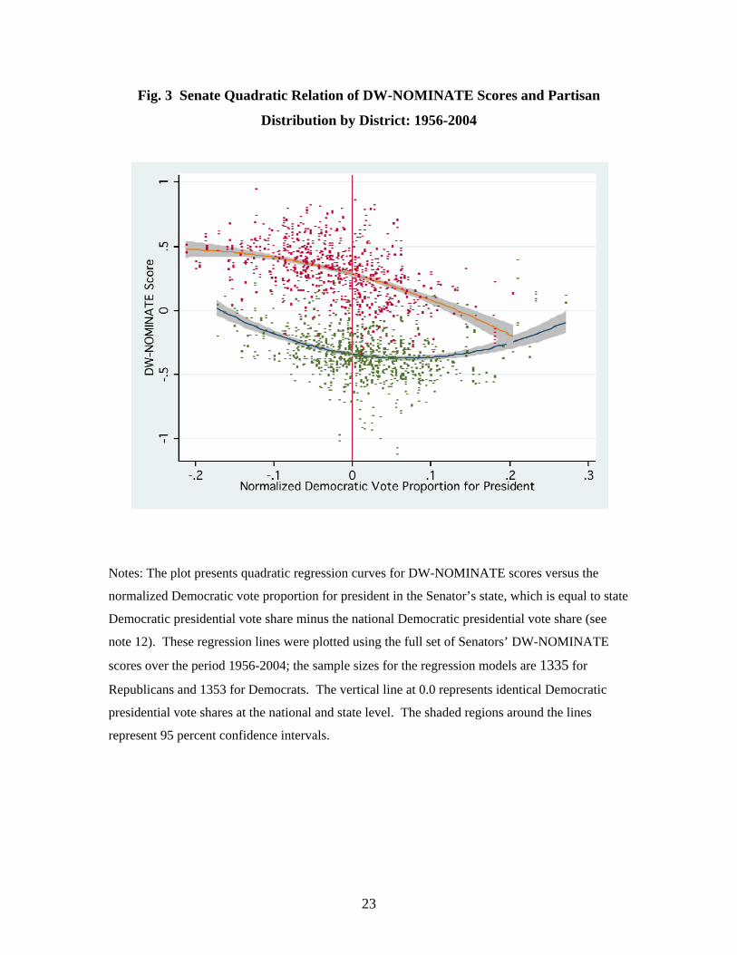
23

Fig. 3 Senate Quadratic Relation of DW-NOMINATE Scores and Partisan

Distribution by District: 1956-2004

Notes: The plot presents quadratic regression curves for DW-NOMINATE scores versus the

normalized Democratic vote proportion for president in the Senator’s state, which is equal to state

Democratic presidential vote share minus the national Democratic presidential vote share (see

note 12). These regression lines were plotted using the full set of Senators’ DW-NOMINATE

scores over the period 1956-2004; the sample sizes for the regression models are 1335 for

Republicans and 1353 for Democrats. The vertical line at 0.0 represents identical Democratic

presidential vote shares at the national and state level. The shaded regions around the lines

represent 95 percent confidence intervals.

24

Fig. 4 Quadratic Regression for the Presidential Vote Share and Ideology for

Senators with Data Separated by Time Periods

Notes: These plots present quadratic regression curves for DW-NOMINATE scores versus the

normalized Democratic vote proportion for president in the Senator’s state, which is equal to state

Democratic presidential vote share minus the national Democratic presidential vote share (see

note 12). The data are the same as in Figure 3, just separated by the eras noted in the figure. The

vertical line at 0.0 represents identical Democratic presidential vote shares at the national and

state level. The shaded regions around the lines represent 95 percent confidence intervals.

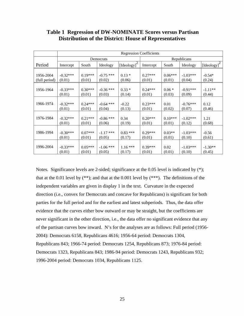
25

Table 1 Regression of DW-NOMINATE Scores versus Partisan Distribution of the District: House of Representatives

Regression Coefficients Period

Democrats Republicans

Intercept

South

Ideology [Ideology]2

Intercept

South

Ideology [Ideology]2 1956-2004 (full period)

-0.32*** (0.01)

0.19*** (0.01)

-0.75 *** (0.02)

0.13 * (0.06)

0.27*** (0.01)

0.06*** (0.01)

-1.03*** (0.04)

-0.54* (0.24)

1956-1964 -0.33***

(0.01) 0.30*** (0.01)

-0.36 *** (0.03)

0.33 * (0.14)

0.24*** (0.01)

0.06 * (0.03)

-0.91*** (0.09)

-1.11** (0.44)

1966-1974 -0.32***

(0.01) 0.24*** (0.01)

-0.64 *** (0.04)

-0.22 (0.13)

0.23*** (0.01)

0.01 (0.02)

-0.76*** (0.07)

0.12 (0.46)

1976-1984 -0.32***

(0.01) 0.21*** (0.01)

-0.86 *** (0.06)

0.34 (0.19)

0.20*** (0.01)

0.10*** (0.01)

-1.02*** (0.12)

1.21 (0.68)

1986-1994 -0.30***

(0.01) 0.07*** (0.01)

-1.17 *** (0.05)

0.83 *** (0.17)

0.29*** (0.01)

0.03** (0.01)

-1.03*** (0.10)

-0.56 (0.61)

1996-2004 -0.33***

(0.01) 0.05*** (0.01)

-1.06 *** (0.05)

1.16 *** (0.17)

0.39*** (0.01)

0.02 (0.01)

-1.03*** (0.10)

-1.30** (0.45)

Notes. Significance levels are 2-sided; significance at the 0.05 level is indicated by (*);

that at the 0.01 level by (**); and that at the 0.001 level by (***). The definitions of the

independent variables are given in display 1 in the text. Curvature in the expected

direction (i.e., convex for Democrats and concave for Republicans) is significant for both

parties for the full period and for the earliest and latest subperiods. Thus, the data offer

evidence that the curves either bow outward or may be straight, but the coefficients are

never significant in the other direction, i.e., the data offer no significant evidence that any

of the partisan curves bow inward. N’s for the analyses are as follows: Full period (1956-

2004): Democrats 6158, Republicans 4616; 1956-64 period: Democrats 1304,

Republicans 843; 1966-74 period: Democrats 1254, Republicans 873; 1976-84 period:

Democrats 1323, Republicans 843; 1986-94 period: Democrats 1243, Republicans 932;

1996-2004 period: Democrats 1034, Republicans 1125.

26

Table 2 Regression of DW-NOMINATE Scores versus Partisan Distribution of the State: Results for the U.S. Senate

Regression Coefficients Period

Democrats Republicans

Intercept

South

Ideology [Ideology]2

Intercept

South

Ideology [Ideology]2 1956-2004 (full period)

-0.39*** (0.01)

0.26*** (0.01)

-0.66 *** (0.07)

4.29 *** (0.54)

0.26*** (0.01)

0.16*** (0.02)

-1.57*** (0.09)

-2.30** (0.81)

1956-1964 -0.39***

(0.03) 0.39*** (0.03)

-0.49 * (0.22)

3.08* (1.32)

0.27*** (0.02)

0.26 ** (0.10)

-0.72** (0.26)

-5.02* (2.50)

1966-1974 -0.38***

(0.01) 0.23*** (0.03)

-0.62 *** (0.15)

2.18* (1.08)

0.19*** (0.02)

0.19*** (0.05)

-2.05*** (0.22)

1.22 (2.04)

1976-1984 -0.37***

(0.01) 0.23*** (0.02)

-0.67 *** (0.11)

5.50*** (1.14)

0.17*** (0.02)

0.28*** (0.03)

-1.59*** (0.21)

2.86 (1.80)

1986-1994 -0.36***

(0.01) 0.13*** (0.02)

-1.05 *** (0.12)

0.47 (1.77)

0.29*** (0.02)

0.09** (0.03)

-1.94*** (0.21)

-5.56* (2.61)

1996-2004 -0.42***

(0.01) 0.16*** (0.02)

-0.95*** (0.12)

3.45 ** (1.23)

0.38*** (0.01)

0.04 (0.02)

-1.63*** (0.15)

-7.48*** (1.16)

Notes. Significance levels are 2-sided; significance at the 0.05 level is indicated by (*);

that at the 0.01 level by (**); and that at the 0.001 level by (***). The definitions of the

independent variables are given in display 1 in the text. Curvature in the expected

direction is significant for both parties for the full period and for the earliest and latest

subperiods. Thus, as for the House, the data offer evidence that the curves either bow

outward or may be straight, but the coefficients are never significant in the other

direction, i.e., there is no evidence that any of the partisan curves bow inward. N’s for

the analyses are as follows: Full period (1956-2004): Democrats 1353, Republicans 1135;

1956-64 period: Democrats 314, Republicans 187; 1966-74 period: Democrats 270,

Republicans 205; 1976-84 period: Democrats 263, Republicans 242; 1986-94 period:

Democrats 272, Republicans 234; 1996-2004 period: Democrats 234, Republicans 267.

27

REFERENCES Adams, James, Thomas Brunell, Bernard Grofman and Samuel Merrill. 2010. Why Candidate Divergence Should be Expected to be Just as Great (or even Greater) in Competitive Seats as in Non-Competitive Ones. Public Choice, 145 (3-4): 417-433. Adams, James and Samuel Merrill. 2003. Voter Turnout and Candidate Strategies in American Elections. Journal of Politics 65(1): 161-189. Adams, James, and Samuel Merrill. 2008. Candidate and Party Strategies in Two-Stage Elections Beginning with a Primary. American Journal of Political Science 52(2): 344-359. Adams, James, Samuel Merrill and Bernard Grofman. 2005. A Unified Theory of Party Competition: A Cross-National Analysis Integrating Spatial and Behavioral Factors. Cambridge: Cambridge University Press. Ansolabehere, Stephen, James Snyder, and Charles Stewart. 2001. Candidate Positioning in U.S. House Elections. American Journal of Political Science 45: 136-59. Bailey, Michael and David Brady. 1998. Heterogeneity and Representation: The Senate and Free Trade. American Journal of Political Science 42: 524-544. Baron, David. 1994. “Electoral Competition with Informed and Uninformed Voters.” American Political Science Review 88 (March): 33-47. Bishin, Benjamin, Jay K. Dow, and James Adams. 2006. Issue representation and diversity in senate elections. Public Choice 129(2): 201-215. Bond, Jon R., Kristin Campbell and James B. Cottrill. 2001. The Puzzle of Constituency Diversity Revisited: Conditional Effects of District Diversity in Congressional Elections.” Manuscript. Texas A&M University. Burden, Barry. 2001. The Polarizing Effects of Congressional Elections. In Peter F. Galderisi (Ed.), Congressional Primaries and the Politics of Representation. New York: Rowman and Littlefield.

Burden, Barry. 2004. Candidate Positioning in US Congressional Elections. British Journal of Political Science 34: 211-227. Butler, Daniel M. 2009. The Effect of the Size of Voting Blocs on Incumbents' Roll-Call Voting and the Asymmetric Polarization of Congress. Legislative Studies Quarterly 34 (3): 297-318. Callander, Steven, and Simon Wilkie. 2007. “Lies, Damned Lies, and Political Campaigns,” with Simon Wilkie. Games and Economic Behavior 60 (August): 262-286.

28

Clinton, Joshua D., Simon Jackman and Douglas Rivers. 2004. The Statistical Analysis of Legislative Behavior: A Unified Approach. American Political Science Review 98(2): 355-370. Downs, Anthony. 1957. An Economic Theory of Democracy. New York: Harper and Row. Erikson, Robert, and David Romero. 1990. Candidate Equilibrium and the Behavioral Model of the Vote. American Political Science Review 84: 1103-1126. Erikson, Robert, and Gerald Wright. 2000. Representation of Constituency Ideology in Congress. In David Brady, John Cogan, and Morris Fiorina (Eds.), Continuity and Change in House Elections (pp. 149-177). Stanford: Stanford University Press. Froman, Lewis A. 1963. Congressmen and Their Constituencies. Chicago: Rand McNally. Gerber, Elizabeth, and Rebecca B. Morton. 1998. Primary Election Systems and Representation. Journal of Law, Economics, and Organization 11(2): 304-324. Griffin, John D. 2006. Electoral Competition and Democratic Responsiveness: A Defense of the Marginality Hypothesis. Journal of Politics 68(4): 911-921. Grofman, Bernard. 2004. Downs and Two-Party Convergence. In N. Polsby (Ed.), Annual Review of Political Science 7: 25-46. Grofman, Bernard and Thomas Brunell. 2001. Explaining the Ideological Differences Between the Two U.S. Senators Elected from the Same State: An Institutional Effects Model. In Peter F. Galderisi (Ed.), Congressional Primaries and the Politics of Representation (pp. 132-142). New York: Rowman and Littlefield Publishers, Inc. Grofman, Bernard, Robert Griffin and Amihai Glazer. 1990. Identical Geography, Different Party: A Natural Experiment on the Magnitude of Party Differences in the U.S. Senate, 1960-84. In R.J. Johnston, F.M. Shelley and P.J. Taylor (Eds.), Developments in Electoral Geography (pp. 207-217). London: Routledge. Grofman, Bernard, Samuel Merrill, Thomas L. Brunell, and William Koetzle. 1999. The Potential Electoral Disadvantages of a Catch-All Party: Ideological Variance Among Republicans and Democrats in the 50 U. S. States. Party Politics 5(2): 199-210. Groseclose, Timothy. 2001. A Model of Candidate Location when One Candidate Has a Valence Advantage. American Journal of Political Science 45(4): 862-886. Jones, David R. 2003. Position-taking and Position Avoidance in the US Senate. Journal of Politics 65(3): 851-863.

29

Kaplan, Noah, David Park, and Travis Ridout. 2006. Dialogue in U.S. Senate Campaigns? An Examination of Issue Discussion in Candidate Television Advertising. American Journal of Political Science 50 (3): 724-736. Kenny, Lawrence and Babak Lotfinia. 2005. Evidence on the Importance of Spatial Models in Presidential Nominations and Elections. Public Choice 123(3): 439-462. Koetzle, William. 1998. The Impact of Constituency Diversity on the Competitiveness of U.S. House Elections, 1962-96. Legislative Studies Quarterly 23: 561-573. Lee David S., Enrico Moretti and Matthew J. Butler. 2004. Do Voters Affect or Elect Policies? Evidence from the U.S. House. Quarterly Journal of Economics 119 (3, August): 807-859. Miller, Gary, and Norman Schofield. 2003. Activists and Partisan Realignment in the United States. American Political Science Review 97: 245-260. Moon, Woojin. 2004. Party Activists, Campaign Resources, and Candidate Position Taking: Theory, Tests, and Applications. British Journal of Political Science 34 (4): 611-633. Ono, Keiko. 2005. Electoral Origins of Partisan Polarization in Congress: Debunking the Myth. Extensions (Fall): 15-20. Owen, Guillermo and Bernard Grofman. 2006. Two-Stage Electoral Competition in Two-Party Contests: Persistent Divergence of Party Positions. Social Choice and Welfare 26: 547-569. Petrocik, John R. 1996. Issue Ownership in Presidential Elections, with a 1980 Case Study. American Journal of Political Science 40(August): 825-850. Poole, Keith T. and Howard Rosenthal. l984. The Polarization of American Politics. Journal of Politics 46: 1061-l079. Schmidt, Amy, Lawrence Kenny, and Rebecca Morton. 1996. Evidence of Electoral Accountability in the U.S. Senate: Are Unfaithful Agents Really Punished? Economic Enquiry 34: 545-67. Schofield, Norman and Gary Miller. 2007. Elections and Activist Coalitions in the United States. American Journal of Political Science. 51, No. 3 (July): pp. 518-531. Schofield, Norman, and Itai Sened. 2006. Multiparty Democracy: Elections and Legislative Politics. Cambridge: Cambridge University Press,

30

Sigelman, Lee, and Emmett H. Buell, Jr. Avoidance or Engagement? Issue Convergence in U.S. Presidential Campaigns, 1960-2000. American Journal of Political Science 48(4): 650-661.

Snyder, James. 1994. Safe Seats, Marginal Seats, and Party Platforms: The Logic of Platform Differentiation. Economics and Politics 6: 201-214. Winer, Stanley, Lawrence Kenny and Bernard Grofman. 2008. Explaining Variation in the Degree of Electoral Competition in a Mature Democracy: U.S. Senate Elections, 1922-2004. Presented at the Annual Meeting of the Public Choice Society, San Antonio, March. Wittman, Donald. 1983. Candidate Motivation: A Synthesis of Alternatives. American Political Science Review 77: 142-157.

1

    

A Heteroscedastic Spatial Model of the Vote:  A Model with Application to the United States 

 Ernesto Calvo 

University of Maryland ecalvo@umd.edu 

 Timothy Hellwig Indiana University 

thellwig@indiana.edu  

Kiyoung Chang University of Maryland 

kiyoung.chang@gmail.com  

       For helpful comments and suggestions, the authors thank Jim Adams, Johanna Birnir, Bernie Grofman, Dan Kselman, Noam Lupu, Sam Merrill, Richard Moore, Vicky Murillo, Bernhard Weßels, and participants at conferences at the Juan March Institute and the Social Science Research Center Berlin (WZB).    

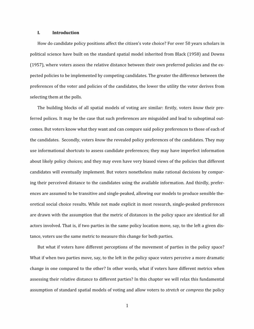
1

I. Introduction 

How do candidate policy positions affect the citizen’s vote choice? For over 50 years scholars in 

political science have built on the standard spatial model inherited from Black (1958) and Downs 

(1957), where voters assess the relative distance between their own preferred policies and the ex‐

pected policies to be implemented by competing candidates. The greater the difference between the 

preferences of the voter and policies of the candidates, the lower the utility the voter derives from 

selecting them at the polls.  

The  building  blocks  of  all  spatial models  of  voting  are  similar:  firstly,  voters know  their  pre‐

ferred polices. It may be the case that such preferences are misguided and lead to suboptimal out‐

comes. But voters know what they want and can compare said policy preferences to those of each of 

the candidates.  Secondly, voters know the revealed policy preferences of the candidates. They may 

use informational shortcuts to assess candidate preferences; they may have imperfect information 

about likely policy choices; and they may even have very biased views of the policies that different 

candidates will eventually implement. But voters nonetheless make rational decisions by compar‐

ing their perceived distance to the candidates using the available information. And thirdly, prefer‐

ences are assumed to be transitive and single‐peaked, allowing our models to produce sensible the‐

oretical social choice results. While not made explicit  in most research, single‐peaked preferences 

are drawn with the assumption that the metric of distances in the policy space are identical for all 

actors involved. That is, if two parties in the same policy location move, say, to the left a given dis‐

tance, voters use the same metric to measure this change for both parties.  

But what  if voters have different perceptions of  the movement of parties  in  the policy space? 

What if when two parties move, say, to the left in the policy space voters perceive a more dramatic 

change in one compared to the other? In other words, what if voters have different metrics when 

assessing their relative distance to different parties? In this chapter we will relax this fundamental 

assumption of standard spatial models of voting and allow voters to stretch or compress the policy 

2

space measuring  the distance  from their preferred policy  location  to  that of different parties and 

candidates. To this end, we propose here a heteroscedastic spatial model of voting, where the per‐

ceived distance from voters to parties is systematically altered by information effects.   

Our emphasis on  informational biases  is directed at observed  inadequacies  in  the existing re‐

search on spatial models of the vote. Previous research has shown that “voters may misestimate the 

policy platforms of candidates or parties either out of ignorance or in a fashion which reflects sys‐

tematic bias”  (Merrill et al.  2001, 200).  In particular,  respondents  tend  to overstate  the  reported 

proximity to parties which they intend to vote for as well as the distance between themselves and 

parties which they will not vote for (Granberg and Brent 1980; Granberg and Jenks 1977; Haddock 

2003). These biases are not trivial and in many cases contribute adversely to the predictive accura‐

cy of spatial models. Empirical tests of proximity voting often find smaller than expected statistical 

effects and yield attenuated parameter magnitudes, even if most analysis validate the general ten‐

ants of the theory. Furthermore, equilibrium positions for parties are often attenuated, resulting in 

models that overestimate centrist positions of parties and candidates. Attenuation biases give rise 

to theoretical problems when trying to ascertain the “correct” location of candidates in policy space 

and, hence, when testing spatial models of voting under misreported proximity. Attenuated proximi‐

ty  estimates  and  centripetal  biases  are  but  one  of  many  puzzles  confronting  scholars  in  recent 

years, as more extensive empirical testing falsifies the theoretical validity of spatial models of vot‐

ing (e.g., Adams and Merrill 1999; Iversen 1994; Rabinowitz and Macdonald 1989).  

Attempts have been made to address the problem. Adams, Merrill, and Grofman (2005), for 

example, propose a “discount” model in which a weight is assigned to recalibrate the effect of prox‐

imity.  Others  have  augmented  existing  spatial  model  to  include  behavioral  factors  (Erikson  and 

Romero  1990)  and  information  in  regards  to  the  candidates’  non‐policy  appeals  (Sanders  et  al. 

2011).  Scholars  also have  looked  to  the  effect  of  political  institutions,  suggesting  that  centripetal 

biases  are moderated  through  the  consideration  of  the distribution of  power  across party  actors 

3

(Kedar 2009).   Electoral rules have also been shown to alter the incentives facing political parties 

(Calvo and Hellwig 2011) and the voter’s perception of party locations (Dahlberg 2012).  More fun‐

damentally, others posit alternative non‐proximity models for how party and candidate policy posi‐

tions enter the vote calculus (Macdonald et al. 2001). Many argue that these solutions improve on 

traditional proximity models.   Yet others have used experimental designs  to show that proximity 

voting rules are,  in  fact, more commonly employed than discounting or directional models (Tomz 

and van Houweling 2008; see also Lacy and Paolino 2010).  

In this chapter our goal is to confront the observed systematic biases in the reported loca‐

tions of parties and candidates.   Working within  the standard spatial model of Black and Downs, 

our emphasis is how information biases contort voter perceptions. The solution we propose allows 

the analyst to model how information biases alter the shape of the policy space used by voters to as­

sess  their proximity  to candidates. Our model allows us  to alter  the perceived distance between  the 

voter and the candidate, allowing the policy space to contract or expand as a function of a variety of 

covariates.  

The chapter proceeds as follows. The next section elaborates on information biases and how 

they are reflected in how voters place candidates in policy space.  We use data from the 1992, 1996, 

and 2008 American presidential elections  to  illustrate  the magnitude of  these  information biases. 

As a motivating example, we draw from the field of optics and conceive of these biases in terms of 

ideological lensing, or magnification. We provide a naïve estimate of the degree of magnification in 

the voters’ perceived ideological distance from themselves to the candidate. Finally, we propose a 

heteroscedastic proximity model of voting where magnification is estimated as a function of behav‐

ioral and candidate specific covariates. Section 4 reports results of estimating the effect of ideologi‐

cal  proximity  on  vote  choice—with  and  without  correcting  for  magnification—using  data  from 

three U.S. presidential elections. Section 5 concludes. 

 

4

II. Voting with Biased Perceptions of Candidate Positions  

Despite decades of research, the literature on how voters decide remains divided by a con‐

ceptual gulf. On the one hand, researchers have developed a rich set of models to explain how ra‐

tional voters make decisions by measuring their relative proximity to the policies proposed by can‐

didates and parties. On the other hand, a large body of research shows that voters are ignorant —

rationally  or  not—  about  politics  and, more  to  the  point,  the  preferences  of  political  candidates 

running for office.   

Contending  models  of  voting  differ  in  important  ways.  Spatial  proximity models  assume 

that voters select among candidates by minimizing the distance from their ideal policy outcome to 

that proposed by each candidate (Downs 1957; Enelow and Hinich 1984). A competing school ar‐

gues that voters are motivated by conviction and prefer candidates that take on more extreme posi‐

tions  (Rabinowitz  and Macdonald 1989).  Finally,  a  third group of  scholars  argue  that  voters  also 

make decisions based on valence‐issues, with candidates or parties building a reputation  for per‐

formance rather than positions (Stokes 1963). Each of these approaches assumes that voters know 

something  about  the  characteristics  of  competing  candidates  for  office—be  it  in  terms  of  policy 

positions, policy extremity, competence/reputation, or some combination thereof. 

The research on political knowledge and voter choice naturally calls into question the valid‐

ity of said proximity based models of vote choice. Indeed, there is a vast American and comparative 

literature documenting information deficits and political naïveté among voters. Describing voters’ 

abilities  to  assimilate  candidate  positions  in  summary  terms,  Converse  (1964)  succinctly  argued 

that Americans are “ideologically innocent.” He showed that very few people could meet the criteria 

of voting on the basis of a liberal‐conservative (or left‐right) scale.   In his seminar work on public 

opinion formation, Zaller (1992) largely echoed Converse’s view.  While the typical voter may know 

something about politics, such knowledge tends to be shallow and ephemeral.  As Zaller (1992, 16) 

puts it, “a majority pays enough attention to public affairs to learn something about it. But even so, 

5

it is easy to underestimate how little typical Americans know about even the most prominent polit‐

ical events – and also how quickly they forget what for a time they do understand.” This view cer‐

tainly calls into question the average American’s ability to cast a vote based on candidate positions 

on one or a set of issues.1   

There  is much  evidence  in  existing  survey  data  to  support  this more  pessimistic  view  of 

voters’ ability to discern and correctly use information about parties and candidates when making 

their decisions. Survey respondents differ in predictable ways when reporting the location of par‐

ties in the ideological space. Respondents with very different political leanings consistently overes‐

timate their distance to parties with which they do not identify as well as the ideological distance to 

parties they do not expect to vote for (Adams et al. 2005; Bartels 1988; Page 1976).  

As an example of this phenomenon, consider voter choice in the 1980, 1996, and 2008 US 

presidential  elections.    In Figure 1 we plot  respondent placements of  the  two major party  candi‐

dates in each of these elections.  The graphs illustrate how respondents’ self‐placements affect their 

view  of  where  the  candidate  is  located  in  policy  space.  Take  as  example  the  task  of  placing  the 

Democratic Party’s  candidate  in 2008, Barack Obama. When asked  in  to place Obama on  the 1‐7 

liberal‐conservative  scale,  a  self‐identified  “extremely  conservative”  respondent  (scored 7  on  the 

scale) places Obama around 6 (5.8) on the scale if she intends to vote for Obama.  A similarly con‐

servative respondent places Obama at  less than 2 (1.7)  if she  instead planned to support another 

candidate.   This can be taken as strong evidence of projection effects: party supporters systemati‐

1 The authors of The American Voter (Campbell et al. 1960) laid out such criteria for voting accord‐ing to issue position.  These include the ability to cognicize the issue in some form (generally inter‐preted as have an opinion on the issue), to perceive where the candidates stand on it, and to see a difference between them.  To this list, Abramson et al. (2009) add that voters must see the positions of the relevant parties or candidates (approximately) correctly if they are to make reasonable deci‐sions. 

6

cally locate the party closer to their own ideal point, while non‐supporters place the party further 

away. 2   

<<Figure 1 about here>> 

We might surmise that such biases due to assimilation and contrast effects shape how vot‐

ers make use of candidates’ placements when making their decision (Adams et al. 2005; Granberg 

and Brent 1980; Granberg and Jenks 1977; Merrill et al. 2001). As we show in the next section, this 

picture implies that individual, candidate, and contextual factors may stretch or compress the policy 

space,  altering  the perceived distance between  the voter  and  the  candidates. Our  contribution  in 

this chapter is to provide a means to model and assess the factors that contribute to what we term 

magnification:  the  curving  of  the policy  space  in  response  to  information.  In  the next  section we 

propose a novel way to incorporate assimilation and contrasting biases into a spatial model of can‐

didate choice. 

 

III. A Motivating  Example  to  describe Magnification  (assimilation  and  contrast)  in 

Policy Distances 

Let us begin with a motivating example for our heteroscedastic spatial model of voting. The in‐

tuition comes from the field of physics, which has developed an extensive literature on gravitational 

lensing: i.e., the effect that matter exerts on a beam of light from a background source as it travels 

across the space towards an observer. The curving of a beam of light passing through a lens alters 

the perceived location of the background source while revealing information about the distribution 

of matter in space. Such altered perceptions apply to politics as well. When it comes to elite‐mass 

2 These biases are not strictly an American phenomenon. For example, British election studies data from 2005 show that when asked to place the Conservative Party on the left‐right scale, a voter located on the far‐right of the left‐right scale identify the Party as very conservative, at approxi‐mately 9 (8.9) 0‐10 point scale if she voted for one of its candidates.  A similarly conservative voter will perceive the Tories as very liberal—at 2.2—if she voted against the party (see Calvo et al. 2012). See also Adams et al.’s (2005, chapter 10) analysis of survey data from France, Norway, and Britain. 

7

communications, the perceived policy position of a political representative is shaped by the location 

of the observer—the observer here being the voter. Drawing from an extensive literature on infor‐

mation bias, we describe similar lensing effects in the perceived location of parties in the ideologi‐

cal space.  

Let us assume that all voters see the location of a party through a convex  lens that projects an 

“image” of the location of the party that differs from its actual location. While we expect all voters to 

observe the party in a single “true” location in the ideological space, spherical aberration3 shifts the 

view of observers so that the image of the party appears closer or further away from its true loca‐

tion.  When voting for a party, the focal point of the object (party or candidate) falls behind the ob‐

ject, which appears  closer  than  it  should. When voting against  the party,  the  focal  point appears 

ahead of the object, which is projected further away than it should. We might think of  the  first of 

these cases as one where the voter is farsighted (unable to focus at a distance); in the second case 

the voter is nearsighted.  

Just as individuals correct their eyesight with lenses, we can speculate that there is a gradu‐

ation of this lens which explains the degree of optical aberration in ideological distances. The curva‐

ture of this lens can be approximated by a large number of different functions, but for the sake of 

our example we can use a simple parabola (e.g. a quadratic approximation) estimating the convexi‐

ty of lenses or the projection of a ray of light on a parabolic mirror.  

As an illustrating example,  let us use the case of the Republican Party in the U.S. In the model   

describes the reported location of the Republican Party by respondent i.  The self‐reported ideolog‐

ical position of the same respondent is given by  . The quadratic approximation is thus   

        .          (1) 

 

3 A convex lens suffers from spherical aberration when light transmitted through the lens fails to converge to a single point.  This is known in optics as hyperopia or, more commonly, as farsighted‐ness. 

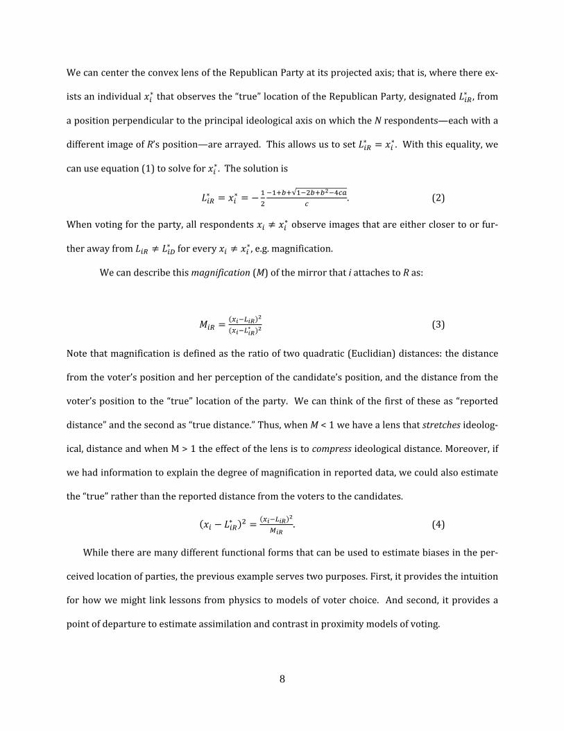
8

We can center the convex lens of the Republican Party at its projected axis; that is, where there ex‐

ists an individual   that observes the “true” location of the Republican Party, designated  , from 

a position perpendicular to the principal ideological axis on which the N respondents—each with a 

different image of R’s position—are arrayed.  This allows us to set  .  With this equality, we 

can use equation (1) to solve for  .  The solution is 

  √ .         (2) 

When voting for the party, all respondents   observe images that are either closer to or fur‐

ther away from   for every  , e.g. magnification.  

We can describe this magnification (M) of the mirror that i attaches to R as: 

 

                     (3) 

Note that magnification is defined as the ratio of two quadratic (Euclidian) distances: the distance 

from the voter’s position and her perception of the candidate’s position, and the distance from the 

voter’s position to the “true” location of the party.   We can think of the first of these as “reported 

distance” and the second as “true distance.” Thus, when M < 1 we have a lens that stretches ideolog‐

ical, distance and when M > 1 the effect of the lens is to compress ideological distance. Moreover, if 

we had information to explain the degree of magnification in reported data, we could also estimate 

the “true” rather than the reported distance from the voters to the candidates.  

      .          (4) 

While there are many different functional forms that can be used to estimate biases in the per‐

ceived location of parties, the previous example serves two purposes. First, it provides the intuition 

for how we might  link  lessons  from physics  to models of voter choice.   And second,  it provides a 

point of departure to estimate assimilation and contrast in proximity models of voting. 

 

9

IV. A Heteroscedastic Proximity Voting Model 

The existing  literature on assimilation and contrast has shown  that reported proximity  to 

parties  is different  for respondents that expect to vote  for or against a party. We can go one step 

further and argue that a number of covariates will explain assimilation and contrast, compressing 

and stretching ideological distances as described in equation 4. Indeed, let us assume that magnifi‐

cation is the result of information processes that can be explicitly modeled with covariates.  

As  it  is  commonly done when  estimating heteroscedastic  discrete models  (e.g., models  in 

which  the  variance  component  is  explained by  covariates  such  as heteroscedastic  probit models, 

negative binomial, etc.), we can assume that the level of magnification in ideological proximity can 

also be  itself a  function of other covariates. We can  therefore use a placeholder parameter    in 

lieu of our magnification term, which will be used to assess the effect of variables that induce mag‐

nification: 

      U VR α 

   .        (5) 

In equation 5 we have substituted the angular magnification estimate with  the exponentiated pa‐

rameter  , so that log  ~ , . Notice that if all covariates for the magnification equation 

have no effect, the  0 1, and equation 5 will be reduced to the standard proximity model.  

  As in the case of a heteroscedastic choice model (Alvarez and Brehm 1995), the expression 

in (5) has the desirable feature of allowing us to model the variance as a linear function of a set of 

covariates. Yet different from a heteroscedastic model, the variance is only rescaling the ideological 

proximity measure.  The second component of the model,  , is a vector of individual‐specific con‐

trols which are unaffected by the covariates for the magnification.  Since the variance applies only 

to distance, we label this a heteroscedastic proximity model.  

By  explicitly  modeling  the  magnification  in  the  ideological  scale,  equation  5  provides  a 

means for testing arguments about which factors, both  individual and systemic, shape the voter’s 

capacity to “see clearly.” In particular, this representation provides a novel way to bring in different 

10

candidate and voter attributes into the spatial model of the vote and, hence, gives us a strategy for 

incorporating those  factors discussed  in the  introduction: non‐proximal (directional) spatial com‐

ponents, candidates’ valence characteristics, and voter attributions.  Let’s consider each of these in 

turn. 

First, take directional effects. Directional models provide an alternative conception of how 

voters  incorporate  information  on party  positions.  First  proposed by Rabinowitz  and Macdonald 

(1989), the directional model has long been the chief rival to the proximity model from within the 

spatial modeling  tradition.  Like  the Downsian proximity model,  the directional model posits  that 

voters obtain utility from candidates’ positions on the issues. This utility is not gained by minimiz‐

ing  proximity  but  is  a  positive  function  of  the  candidate’s  distance  from  the  voter.    Specifically, 

when candidates are on opposite sides of the neutral point, N, directional voters prefer the candi‐

date who  advocates  their  side.  In  the  context  of  American  politics,  voters  select  the  larger  from 

(  and ( .  

The explanatory power of directional models relative to the Downsian proximity model has 

been much contested, and with mixed results.4 Tests of the two models, however, have compared 

them directly, with each component affecting voter utility directly and in additive fashion.  Conclu‐

sions  in  favor of one or  the other often hinge on how analysts measure voter utility or on which 

modeling assumptions are relaxed (see Lewis and King 1999). Mixed findings aside, directional and 

proximity effects are typically pitted against one another within the context of a mean model.  Tests 

between rival models are thus on the order of a horse race between variables as analysts discern 

whether  proximity  of  directional  components  carry  greater weight.  Our  approach  is  different.  It 

uses information on the extremity of where respondents place candidates as shaping the degree of 

angular magnification, rather than on affecting directly the choice model.   4 Recent research, however, has used experimental designs to get around previous measurement problems and finds stronger support for the proximity view (Tomz and van Houweling 2008; Lacy and Paolino 2010).  We take this as instructive evidence for using direction extremity to modify ideological lensing arising from proximity models, rather than the other way around. 

11

Next, consider valence. Our model of ideological lensing provides a new strategy for incor‐

porating candidates’ non‐policy appeals. A great deal of recent scholarship has emphasized the im‐

portance of parties’ non‐positional related reputations with respect to competence,  integrity, cha‐

risma, and the like (Adams et al. 2005; Clarke et al. 2009; Schofield and Sened 2006). These studies 

demonstrate that the inclusion of non‐proximity components into the random utility model yields 

more complete models  for understanding election outcomes and how party strategies respond to 

voter preferences. We build on this  insight. However, rather than incorporating party valence ad‐

vantages additively, we explore whether valence evaluations bias voters’ perceptions of where the 

party is positioned in ideological space. We know from previous work that valence advantages al‐

low parties to attain larger shares of the vote than they would as predicted solely by spatial consid‐

erations.5 But voters’ assessment of a party’s location in policy space, on the one hand, and its va‐

lence (dis)advantage, on the other hand, are typically assumed to be unrelated to one another.6 Fur‐

ther, the spatial modeling literature generally assumes that parties’ valence advantages are identi‐

cal across voters. 

We relax these assumptions. We model the degree of bias in voter assessments of party po‐

sitions as a function of the voter’s perception of the party’s valence appeals. We maintain that if a 

voter  i views  the  image of a party R  as proximally closer  to her  than R’s actual  location,  then  the 

degree of magnification, M, should decrease. With reference to equation 4, this makes it likely that 

. To the extent that reputational considerations are built on familiarity, this 

claim finds support in work on voter choice out of the behavioral tradition which shows that voters 

dislike uncertainty and resist supporting parties they know little about (even if they share the par‐

5 See especially Adams et al.’s (2005) unified model; also see Wittman (1983), Groseclose (2001), Calvo and Hellwig (2011). 6 Something of an exception is Sanders et al. (2011) who model valence as a function of voter‐party issue proximity, thus positing that spatial effects shape utility indirectly, through valence character‐istics. 

12

ty’s  policy preferences).7  Parties who  voters  view  as being more  competent,  trustworthy,  charis‐

matic, and the like, should receive a biased evaluation by the voter in positional terms (that is, the 

distance between   and   is small). Lastly, the heteroscedastic proximity model provides a way to 

model how the effect of voter perceptions of candidate location on the vote is altered by the indi‐

vidual’s acquisition of information about politics.  As noted above, there exists a large and generally 

uncontested  literature  highlighting  the  dearth  of  Americans’  objective  knowledge  about  political 

institutions  and  affairs  (Converse  1964;  Delli  Carpini  and  Keeter  1996).  More  contested  among 

scholars is whether such information discrepancies matter for voter choice and, by extension, elec‐

tion outcomes. Perhaps not surprisingly, researchers have sought out different pathways through 

which  information  effects  are  present  (Gomez  and  Wilson  2001;  Zaller  2004).    Using  our 

heteroscedastic proximity model, we examine whether exposure to information about politics mat‐

ters for voter choice by sharpening, or “clarifying,” the influence of ideological distance. 

With this information, the heteroscedastic proximity model is as shown in equation (5) with de‐

sirable feature of allowing us to model the variance,  , specified as a linear function of policy ex‐

tremism, valence, and political information, expressed as 

 

        .      (6) 

 

In equation 6,   represents voter i’s perception of the extremity of R's policy preferences,   is i’s 

assessment of R’s non‐positional qualities, or valence characteristics,   represents  i’s exposure to 

political  information,  and  the  s  are  parameters  to  be  estimated.  The  directional  effect,  ,  is 

scored 1 if the voter places the candidate as more extreme but on the same side of the neutral point 

as herself,  and 0 otherwise.    Valence,  ,  is  coded +1  if  the  respondent  likes  anything  about  the 

7 See, among others, Alvarez (1997) and Bartels (1996).  Enelow and Hinich’s (1981) formal model yields consistent predictions. 

13

presidential  candidate’s  party,  ‐1  if  she  dislikes  anything  about  the  party,  and  0  otherwise.8  The 

political information variable, , is a subjective measure of how much attention the respondent pays 

to news about government and politics.9 Finally, note that we control for the respondent’s partisan 

dispositions using the standard ANES seven‐point scale for party identification.  This is entered into 

the specification in equation 5 as part of  , the vector of controls. 

We estimate a set of heteroscedastic proximity models—one each for U.S. presidential elec‐

tions in 1980, 1996, and 2008—using the Markov Chain Monte Carlo (MCMC) engine in WinBUGS 

(Spiegelthaler et al. 2003).  We estimate two equations – one for the choice model and the other for 

the variance component.   The choice model  is  further split between the vector of exogenous con‐

trols (party identification), BZ, and the ideological distance component,  .  

Table 1 presents the model results: the choice model includes the estimated effect of ideo‐

logical distance on  the  likelihood  the respondent selects  the candidate. The choice‐specific coeffi‐

cients  for  partisanship  are  positively  signed  and  precisely  estimated  in  each  case.    Our  interest, 

however, lies with the results for ideological distance.  Here, we observe differences in the effect of 

positional proximity  in models  that do model  the variance  as  a  function of  ideological  extremity, 

valence, and information (Models 2, 4, 6) and those that do not (Models 1, 3, 5).  When the variance 

model is left unspecified, parameter estimates on Ideological Distance, while negatively signed, are 

imprecisely  estimated.   However, when we do  specify  the variance,  these estimates  in  the  choice 

model attain statistical significance. This finding holds across the 1980, 1996, and 2008 elections.  

The remaining covariates pertaining to directional, valence, and information effects are specified to 

8 Specifically, the American National Election Studies surveys ask respondents to identify whether there is anything they like about the Democratic and Republican Parties.  This is followed by an item asking whether there is anything they dislike about the two main parties. With responses to these two binary choice items, we construct a three‐point scale scored ‐1 dislike only, 0 for neither like nor dislike, or both like and dislike, and +1 for like only.   9 The measure is coded 1 = “don’t pay much attention,” 2 = “pay some attention,” 3 = “pay a great deal of attention.” 

14

account for variations about the voter’s decision with respect to ideological proximity.  We consider 

each in turn. 

<<Table 1 about here>> 

 

Explaining the Effect of Candidate Extremity on Proximity Voting 

First consider the influence of directional effects. The heteroscedastic specification implies 

that the ideological space is stretched so that candidates’ distance to voters differs as they move to 

the extreme or  to  the center of  the  ideological space. A positively signed coefficient on  the direc‐

tional term would indicate ideological distance matters less when that when the candidate is more 

extreme  than  the voter,  and on  the same side of N,  than otherwise. A negative sign, on  the other 

hand, means that the penalty attached to the non‐proximal candidates is greater.  That is, while the 

proximity model attaches a penalty  to candidate R when    is  far  from  ,  the magnitude of  that 

penalty is greater if  0.  Table 1 shows that this is in fact the case for the 1980 and 1996 elec‐

tions.  In these cases, voters who viewed the candidate as more extreme than themselves put great‐

er  (negative)  weight  on  ideological  distance  than  voters  who  did  not.    In  terms  of  ideological 

lensing, the directional effect stretches the distance between the voter and the candidates. This sto‐

ry does not  apply,  however,  to  the 2008 election.    In  this  case,    is  indistinguishable  from zero, 

meaning that extremely placed candidates receive no penalty on policy terms.   

These  results  suggest  that  in  1980,  a  typical  voter  i  was  less  and  less  likely  to  support 

Ronald Reagan or Jimmy Carter for president as a function of how extreme he viewed the particular 

candidate’s ideology to be. In 1980 the large and precisely estimated coefficient on Directional Ef­

fect indicates that she assigns a relatively heavy penalty on extreme position‐taking candidates. The 

same story applies to 1996.   The negatively signed coefficient on the directional  term in the vari‐

ance equation implies that proximity voters punished the candidates, Bob Dole and Bill Clinton, for 

taking what  they  perceived  as  extreme  positions.    However,  the  “extremity  penalty”  confronting 

15

Dole and Clinton  in 1996 was  less  than  that  facing Reagan and Carter  in 1980, as evinced by  the 

relative sizes of the coefficients.  And by 2008, this penalty had altogether disappeared: taking ex‐

treme positions (on the preferred side of the neutral point) had no adverse effect on proximity vot‐

ing.  We can infer from this result that the candidates in 2008, John McCain and Barack Obama, did 

not suffer from coming across as either too conservative or too liberal or conservative the way their 

predecessors did. 

 

Explaining the Effect of Valence on Proximity Voting 

Next consider valence effects. Unlike the directional effect, coefficients estimated for the va‐

lence parameters are consistent across elections:  in 1980, 1996, and 2008,  the estimate on Party 

Valence is positively signed and statistically significant. In terms of the heteroscedastic model, this 

means that as valence increases, the voter’s perceived ideological distance, , shrinks.  Put 

differently, as  the distance between the voter’s preferred policy  location and that of  the party  in‐

creases, higher valence makes the distance smaller and the disutility smaller. As a party’s valence 

advantage goes up, the effect of ideological distance on the vote becomes smaller. In the extreme, if 

valence is sufficiently high, a voter will perceive that the candidate is “right next to her,” irrespec‐

tive of the policy proposed, and the utility of spatial proximity voting will remain constant. In effect, 

as a candidate’s valence advantage approaches its maximum, he becomes spatially closer to each and 

every voter in the population. 

Figure 2 illustrates this effect for a moderately liberal voter (located at 3 on 1‐7 scale) using 

parameter estimates from Model 6 in Table 1 for the 2008 election.  If the candidate is also located 

at 3, then i prefers the candidate with equally high probability (~0.63) regardless of its valence lev‐

el.10  But as the candidate moves away from i’s preferred location, it loses less utility if it is deemed 

to have high valence (solid line) than if it has low valence (dashed line). Notice that this interpreta‐

10 In this illustration, the other candidate in the two-candidate race is placed at 5 on the 1-7 scale.

16

tion shows that  the effect of high valence  is  to “drown out” spatial proximity as a determinant of 

voting. By contrast, as valence declines, the effect of spatial proximity becomes more pronounced.  

<<Figure 2 about here>> 

The intuition is straightforward and surprising: voters will perceive low valence parties as 

ideological and high valence parties as pragmatic, irrespective of their actual policy location. In oth‐

er words, voters who attach high valence marks to their party will see them close to themselves and 

pragmatic, while parties with low valence will appear further removed and much more ideological. 

Again, this trait remains constant in all model results. 

 

Attention to News and Ideological Distance 

Finally, consider information effects, captured in our models as attention to political news.  

Many researchers have sought to ascertain the influence of political information on an individual’s 

voting behavior. We examine what effect, if any, information acquisition has on ideological lensing.  

The same logic applies as above: a positive coefficient on the information variable in the variance 

component implies that ideological distance is compressed, or that ideology matters for voter utility 

among informed individuals.   A negative coefficient, on the other hand, implies that the politically 

informed are more likely to use ideological proximity to inform their vote—in this case, information 

stretches distance. Results show that that our information measure, Attention to News, does not ex‐

ert the same general effect across the three elections.  In the 1980 and 1996 polls, attention to news 

had no biasing effect on Ideological Distance.  In 2008, however, the coefficient on Attention to News 

is precisely estimated and negatively signed.  This means that among those located proximally close 

to a candidate (say Barack Obama), the utility of voting for Obama was greater as information levels 

increased. This utility, however declines rapidly among the informed as the candidate moves away 

from  the  voter,  i.e.,  as    increases.  Among  the  less  informed  ideology matters  less:  the 

gains from proximally  located candidates are  lower but so are the losses  incurred by moving fur‐

17

ther away on  the  ideological  continuum. Figure 3  illustrates  this dynamic,  again using parameter 

estimates from the 2008 election. We again set   3.   

<<Figure 3 here>> 

Taken together, the results of these heteroscedastic proximity models provide insights into 

American presidential politics. Voters in the United States do select candidates to the office of pres‐

ident based policy (ideological) considerations. The voter’s view of the candidates’ policy positions, 

however,  is  highly  biased,  particularly  but  not  exclusively  among  those  at  self‐identify  at  the  ex‐

treme positions on the liberal‐conservative scale (see Figure 1).  And once we model the “shape” of 

this lensing effect, ideological distance becomes a stronger predictor of voter utility (Table 1).  Yet 

perhaps of greatest interest to students of American politics come from when we model the lensing 

effects via the heteroscedastic proximity model of voter utility.   Comparing the voter’s calculus in 

the 1980, 1996, and 2008 elections, we uncover a mix of continuity and change.  Not surprisingly, 

partisanship  and  ideology matter,  and  do  so  consistently.  Candidates’  non‐positional  valence  ap‐

peals, with respect to competence, integrity, and the like, also matter across elections—yet we pro‐

vide a novel means for showing how valence blunts the proximity effect.  

 

V. Concluding Remarks  

The  assumptions  undergirding  spatial models  of  voting  are  by  now  familiar:  1)  voters  know 

their preferred polices; 2) voters know the revealed policy preferences of candidates; and 3) voter 

preferences  are  transitive  and  single‐peaked.  Employing  a  novel heteroscedastic proximity model, 

we are able to relax these assumptions. In particular, we allow voters to use different metrics when 

measuring  their  relative  proximity  to  parties.  Furthermore,  we  show  that  information  effects 

stretch  and  compress  the  policy  space  in  systematic  ways.  While  we  have  not  been  the  first  to 

acknowledge  this  perceptual  bias  in  the  voters’  perceptions,  our work  offers  a more  cogent  and 

theoretically informed way (a) to measure ideological lensing and (b) to correct for it.  

18

By allowing spatial distances to vary in response to changes in information, our heteroscedastic 

proximity  approach  is  able  to  explain  attenuation  biases  in  current  proximity  models  of  voting. 

Drawing on insights from physics, this research sheds new light on the problems of—and offer solu‐

tions  to—ideological  lensing  in  elections.  Borrowing  from  lens models  in  optics, we  assume  that 

individuals observe the image of a party located in the ideological space rather than the actual loca‐

tion of a party.   

In this chapter, we applied the heteroscedastic proximity model to three presidential elec‐

tions in the United States. As a means to correct for—or make adjustments to—ideological aberra‐

tion, we model  the  level  of  angular magnification  in proximity  voting  via  a  trio  of  non‐proximity 

covariates.    Our model  of magnification  includes  a  directional  component,  a  valence  component, 

and an information component. Using this heteroscedastic proximity model, we show that the direc‐

tional component and the  information component both vary across electoral contests.   Regarding 

direction, our three‐period analysis shows that the penalty of candidates’ taking extreme positions 

as declined over time.  Indeed, the size of the coefficient on the directional effect,  , is half as great 

in 1996 as in 1980, and by 2008 is essentially zero.  This trend suggests that while presidential can‐

didates used to be penalized by taking extreme positions on the issues, such penalties have declined 

with  time.    This  tendency  comports with  a  general  sentiment  that American politics  has become 

polarized and that such polarization is electorally sustainable (McCarty et al. 2005). As for political 

information, our results imply that in earlier periods, access to information had no effect in terms of 

enhancing  (stretching)  or  blunting  (compressing)  the  effects  of  voter  and  candidate  policy  posi‐

tions.  However, in the recent 2008 election, proximity voting was stronger among the more politi‐

cally  informed.    Both  of  these  changes  comport with  common  characterizations  of  the  changing, 

increasingly volatile nature of presidential politics in the United States.  

Future work on elections in the U.S. and elsewhere should might extend and improve upon 

the framework we have provided. For example, extrapolating from current trends, it might be the 

19

case that the heteroscedastic proximity model applied to the 2012 U.S. election would yield a posi‐

tive  coefficient  on  the  directional  parameter,  indicating  that  proximity  voting  is  greater  among 

those perceiving candidates as more extreme. Future work might also distinguish among different 

sources of political information.  Are viewers of more politically charged news outlets like Fox News 

or MSNBC more likely to vote on the basis of ideological proximity than those receiving information 

from  other  sources?  In  short,  our  contribution  has  provided  a  tool  for  systematically  comparing 

these  effects  across  elections  and,  in  turn,  a means  for  deepening  our  understanding  about  how 

voters decide.   

 

   

20

References 

Abramson, Paul R., John Aldrich, and David W. Rohde. 2009. Change and Continuity in the 

2008 Elections. Washington D.C.: CQ press. 

Adams, James, and Samuel Merrill III. 1999. “Modeling Party Strategies and Policy Repre‐

sentation in Multiparty Elections: Why are Strategies so Extreme?” American Journal of Political 

Science 43: 765‐91. 

Adams, James, Samuel Merrill III, and Bernard Grofman. 2005. A Unified Theory of Party 

Competition. New York: Cambridge University Press. 

Alvarez, R. Michael. 1997. Information and Elections. Ann Arbor: University of Michigan 

Press. 

  Alvarez, R. Michael, and John Brehm. 1995. “American Ambivalence Toward Abortion Poli‐

cy: Development of a Heteroskedastic Probit Model of Competing Values.” American Journal of Polit­

ical Science. 

Bartels, Larry. 1988. Presidential Primaries and the Dynamics of Public Choice. Princeton, NY: 

Princeton University Press. 

Bartels, Larry. 1996. “Uninformed Votes: Information Effects in Presidential Elections.” 

American Journal of Political Science 40: 194‐220. 

  Black, Duncan. 1958. The Theory of Committees and Elections. New York: Cambridge Univer‐

sity Press. 

Calvo, Ernesto, and Timothy Hellwig. 2011. “Centripetal and Centrifugal Incentives under 

Different Electoral Systems.” American Journal of Political Science. 55(1): 27‐41. 

Calvo, Ernesto, Timothy Hellwig, and Kiyoung Chang. 2012. “The Eye of the Beholder: Ideo‐

logical Lensing, Information Effects, and the Vote.” Paper presented Paper prepared for the confer‐

ence “Contemporary Applications of the Spatial Model,” Instituto Juan March, 27 April 2012. 

21

Campbell, Angus, Philip Converse, Warren Miller, and Donald Stokes. 1960. The American 

Voter. New York: Wiley. 

Clarke, Harold D., David Sanders, Marianne C. Stewart, and Paul F. Whiteley. 2009. Perfor­

mance Politics and the British Voter. Cambridge: Cambridge University Press. 

Converse, Philip. 1964. “The Nature of Belief Systems in Mass Publics.” In Ideology and Dis­

content, ed. David Apter. New York: Free Press. pp. 206‐261. 

Dahlberg, Stefan. 2012. “Does Context Matter? The Impact of Electoral Systems, Political 

Parties and Individual Characteristics on Voters’ Perceptions of Party Positions.” Unpublished man‐

uscript, University of Gothenburg. 

Delli Carpini, Michael, and Scott Keeter. 1996. What Americans Know about Politics and Why 

It Matters. New Haven, CT: Yale University Press. 

Downs, Anthony.  1957. An Economic Theory of Democracy. New York: Harper and Row. 

Enelow, James M, and Melvin J. Hinich. 1981. “A New Approach to Voter Uncertainty in the 

Downsian Spatial Model.” American Journal of Political Science 25(3): 483‐93. 

Enelow, James M, and Melvin J. Hinich. 1984. The Spatial Theory of Voting: An Introduction. 

New York: Cambridge University Press. 

Erikson, Robert, and David Romero. 1990. “Candidate Equilibrium and the Behavioral Mod‐

el of the Vote.” American Political Science Review 84: 1103‐26. 

Granberg, Donald, and Edward Brent. 1980. "Perceptions of Issue Positions of Presidential 

Candidates: Candidates are often perceived by their supporters as holding positions on the issues 

that are closer to the supporters' views than they really are." American Scientist no. 68 (6):617‐625. 

Granberg, Donald, and Richard Jenks. 1977. "Assimilation and Contrast Effects in the 1972 

Election." Human Relations no. 30 (7):623‐640. 

22

Gomez, Brad T., and J. Matthew Wilson.  2001.  “Political Sophistication and Economic Vot‐

ing in the American Electorate: A Theory of Heterogeneous Attribution.” American Journal of Politi­

cal Science  45 (October): 899‐914. 

Groseclose, Tim. 2001. “A Model of Candidate Location When One Candidate Has a Valence 

Advantage” American Journal of Political Science. 45 (October): 862‐86. 

Haddock, Geoffrey. 2003. "Making a Party Leader Less of a Party Member: The Impact of 

Ambivalence on Assimilation and Contrast Effects in Political Party Attitudes." Political Psychology 

no. 24 (4):769‐780. 

Iversen, Torben. 1994. “Political Leadership and Representation in Western European De‐

mocracies: A Test of Three Models of Voting.” American Journal of Political Science 38: 45‐74. 

Kedar, Orit. 2009. Voting for Policy, Not Parties. New York: Cambridge University Press. 

Lacy, Dean, and Philip Paolino. 2010. “Testing Proximity versus Directional Voting using Ex‐

periments.” Electoral Studies 29(3): 460‐71. 

Lewis, Jeffrey B., and Gary King. 1999. “No Evidence on Directional vs. Proximity Voting.” Po­

litical Analysis 8(1): 21‐33. 

Macdonald, Stuart Elaine, George Rabinowitz, and Ola Listhaug. 2001. “Sophistry versus Sci‐

ence: On Further Efforts to Rehabilitate the Proximity Model.” Journal of Politics 63(2): 482‐500. 

McCarty, Nolan, Keith Poole, and Howard Rosenthal. 2005. Polarized America: The Dance of 

Ideology and Unequal Riches. Cambridge, MA: MIT Press. 

  Merrill, Samuel III, Bernard Grofman, and James Adams. 2001. “Assimilation and Contrast 

Effects in Voter Projections of Party Locations: Evidence from Norway, France and the USA.” Euro­

pean Journal of Political Research 40(2): 199‐221. 

Page, Benjamin I. 1976. “The Theory of Political Ambiguity.” American Political Science Re­

view 70(3): 742‐52. 

23

Rabinowitz, George, and Stuart Elaine McDonald. 1989. “A Directional Theory of Issue Vot‐

ing.” American Political Science Review 83: 93‐121. 

Sanders, David, Harold D. Clarke, Marianne C. Stewart, and Paul Whiteley. 2011. “Downs, 

Stokes, and the Dynamics of Electoral Choice.” British Journal of Political Science 41(3): 287‐314. 

Schofield, Norman, and Itai Sened. 2006. Multiparty Democracy: Elections and Legislative 

Politics. New York: Cambridge University Press. 

Spiegelhalter, David, Andrew Thomas, Nicky Best, Dave Lunn. 2003. WinBUGS user Manual 

1.4, Cambridge UK. {http://www.mrc‐bsu.cam.ac.uk/bugs}.Stokes, Donald. 1963. “Spatial Models of 

Party Competition.” American Political Science Review 57: 368‐77. 

Tomz, Michael, and Robert P. van Houweling. 2008. “Candidate Positioning and Voter 

Choice.” American Political Science Review 102(3): 303‐318. 

Wittman, Donald. 1983. “Candidate Motivation: A Synthesis." American Political Science Re­

view 142‐57. 

Zaller, John R. 1992. The Nature and Origins of Mass Opinion. New York: Cambridge Universi‐

ty Press. 

Zaller, John R. 2004. “Floating Voters in U.S. Presidential Elections, 1948‐2000.” In W.E. Sa‐

ris and P.M. Sniderman, eds., Studies in Public Opinion: Attitudes, Nonattitudes, Measurement Error, 

and Change. Princeton, NJ: Princeton University Press. 

 

 

   

24

 Table 1.  Heteroscedastic Proximity models  

   1  2  3  4  5  6 

  1980  1980  1996  1996  2008  2008 Choice Model             Ideological Distance  ‐0.068  ‐0.067  ‐0.065  ‐0.190  ‐0.056  ‐0.039   (0.746)  (0.018)***  (0.302)  (0.033)***  (0.060)  (0.010)*** Party Identification  0.029  0.040  0.071  0.094  0.096  0.099   (0.009)**  (0.009)***  (0.008)***  (0.009)***  (0.008)***  (0.011)*** Constant  ‐0.290    ‐0.750    ‐0.594     (10.973)    (4.656)    (1.080)   Ideological Vari‐ance Model 

           

Directional Effect    ‐0.811    ‐0.398    ‐0.028     (0.171)***    (0.118)**    (0.198) Party Valence    0.747    0.698    1.252     (0.092)***    (0.101)***    (0.132)*** Attention to News    ‐0.088    0.078    ‐0.210     (0.099)    (0.046)+    (0.067)** LogLik  ‐1102.1  ‐998.7  ‐1389.2  ‐1075.8  ‐1717.4  ‐753.1 N  1838  1736  2570  2076  3064  1418 

 Notes: Cells report coefficients and standard errors from estimating heteroscedastic proximity model described in the text. ***p<0.001, **p<0.01, *p<0.05, +p<0.1, two‐tailed tests. Source: American National Election Studies.     

25

Figure 1. Mean Candidate Placements versus Self­Placements, US 1980, 1996, 2008 

   

   

   

1

2

3

4

5

6

1 2 3 4 5 6 7Mean cand

idate placem

ent

Self‐placement

Carter 1980

2

3

4

5

6

7

1 2 3 4 5 6 7Mean cand

idate placem

ent

Self‐placement

Reagan 1980

1

2

3

4

5

6

1 2 3 4 5 6 7

Mean cand

idate placem

ent

Self‐placement

Clinton 1996

2

3

4

5

6

7

1 2 3 4 5 6 7Mean cand

idate placem

ent

Self‐placement

Dole 1996

1

2

3

4

5

6

1 2 3 4 5 6 7Mean cand

idate placem

ent

Self‐placement

Obama 2008

2

3

4

5

6

7

1 2 3 4 5 6 7

Mean cand

idate placem

ent

Self‐placement

McCain 2008

26

Notes: solid lines report mean candidate placements among candidate supporters, dashed lines report mean candidate placements among non‐supporters.  Means with 10 or fewer respondents not reported. Source: American National Election Studies.     

27

Figure 2. The Effect of Party Valence in the Heteroscedastic Proximity Model  

  Notes: Figure displays the probability voter i intends to vote for a candidate as the candidate moves in policy space.  Voter i is located at 3 on the 1‐7 ideology scale.  The other candidate (not shown) is located at position 5.  The figure indicates how the candidate’s position as perceived by i (horizon‐tal axis) and i’s perceived valence of the candidate’s party (solid and dashed lines) affect the proba‐bility i supports the candidate. Simulated probabilities are based on parameter estimates from Ta‐ble 1 Model 6 for the 2008 U.S. presidential election.     

28

Figure 3. The Effect of Information (Attention to News) in the Heteroscedastic Proximity Model 

 

  

Notes: Figure displays the probability voter i intends to vote for a candidate as the candidate moves in policy space.  Voter i is located at 3 on the 1‐7 ideology scale.  The other candidate (not shown) is located at position 5.  The figure indicates how the candidate’s position as perceived by i (horizon‐tal axis) and i’s level of attention to news (solid and dashed lines) affect the probability i supports the candidate. Simulated probabilities are based on parameter estimates from Table 1 Model 6 for the 2008 U.S. presidential election.  

Inferring Ideological Ambiguity from Survey Data

Arturas Rozenas∗

∗I am grateful to John Aldrich, Scott Desposato, Jeremy Reiter, Fan Li, Mitchell Seligson, and James Stimsonfor comments and suggestions.

1. INTRODUCTION

It has become conventional wisdom to think of electoral competition in terms of parties takingpositions on policy issues and voters choosing their representatives based on those positions. Quiteoften, however, instead of communicating clear platforms, politicians make contradicting policystatements, remain ambiguous about details or avoid talking about issues altogether. For example,Mitt Romney, a presidential candidate in the U.S. 2012 elections, has been constantly accusedof remaining too vague on key policy issues.1 In the 2008 presidential campaign, Barack Obamapromised to withdraw the U.S. troops from Iraq within 16 months whereas John McCain proposedfar more ambiguous plan to remain in Iraq for “up to 100 years.”2

To explain ideological ambiguity, spatial theorists have referred to risk-attitudes of the voters(Shepsle, 1972), the desire of politicians to avoid divisive issues (Page, 1976), context-dependenceof voting decisions (Callander and Wilson, 2008), uncertainty of the candidates(Glazer, 1990), orstrategic benefits of not committing to a certain platform (Alesina and Cukierman, 1990; Aldrich,1995). Empirical research, on the other hand, focused mostly on voting behavior finding thataccounting for ideological ambiguity improves predictions of the standard spatial voting models(Alvarez, 1997; Bartels, 1986; Campbell, 1983a,b; Tomz and van Houweling, 2009).

These examples suggest theoretical and empirical reasons to treat policy platforms not as pointsbut as probability distributions over policy space. Indeed, the notion of policy platforms as pointshas a very limited reach. For example, it cannot be applied to study policy positions of decentralizedpolitical parties involving a variety of activists with diverse policy preferences (Aldrich, 1983; Millerand Schofield, 2003). Another case concerns developing democracies, where, for many reasons,parties are known to lack defined ideological positions(Evans and Whitefield, 2000; Kitschelt et al.,1999; Mainwaring, 1995; Scully, 1995). If policy positions are defined as points, it is not clear whatit means for a party or a candidate not to have a position. Conceptualizing policy position as aprobability distribution provides a more general approach to empirical study of party competition:a “no position” platform can be described by a highly dispersed distribution whereas a platform asa point can be defined as a distribution with a vanishingly small dispersion.

Although there are multiple reasons to study ideological ambiguity, efficient tools to measurethis quantity are lacking. The existing scholarship on the measurement of policy positions operatesunder the assumption that these positions are points, often even referred to as as ‘ideal points’(Ansolabehere, Snyder Jr and Stewart III, 2001; Clinton and Jackman, 2004; Laver, Benoit andGarry, 2003; Martin and Quinn, 2002). This paper presents a statistical model to estimate ideo-logical ambiguity from survey data (e.g., opinion polls or expert surveys) – the kind of data that iswidely available in terms of temporal depth and geographical width.

1For example, “Where are Mitt Romneys details?”, by Scott Lehigh, Boston Globe, June 27, 20122‘Obama Fuels Pullout Debate With Remarks’, New York Times, July 4, 2008.

1

2. SURVEY DATA AND AMBIGUITY MEASUREMENT

The existing literature offers two approaches for measuring ideological ambiguity. The first approachuses direct measures by asking respondents to report their uncertainty about the position of a givencandidate (Alvarez, 1997) or by asking them to place political actors on a scale in a form of aninterval rather than a point (Tomz and van Houweling, 2009). Unfortunately, such surveys are raremaking it difficult to use these approaches for a systematic study of ideological ambiguity, especiallyin a cross-national context.

Another approach is to use indirect methods where ambiguity is inferred either from disagree-ment among the respondents (Campbell, 1983a,b) or from the patterns in the missing survey data(Bartels, 1986). These indirect methods can be applied to many data sets, which ask citizens orpolitical experts to place political parties on a policy scale. However, a naive application of theseapproaches is wanting, as I discuss now.

2.1. Interpreting Respondent Disagreement

Every survey where respondents are asked to place political candidates on issue scales generatesvariation in judgments. It appears intuitive to use the sample standard deviation of the placementsσ as an estimate of a party’s ideological ambiguity as suggested by Campbell (1983a,b). However,the intuition is flawed on several levels. First, a high degree of disagreement between the respondents(and hence high σ) may indicate the lack of information on the part of respondents (Marks et al.,2007) or an intrinsic ambiguity of a party’s policy position Campbell (1983a,b). Thus, to correctlyestimate ideological ambiguity, we have to disentangle the respondent-level and party-level effectson the observed respondent disagreement.

Second, respondent disagreement might occur due to the scale-heterogeneity effect: even if aparty is not ambiguous and respondents are well-informed, they might provide conflicting place-ments due to different interpretation of the measurement scale. Treating disagreement amongrespondents without proper adjustments for the scaling effects can result in faulty inference aboutideological ambiguity.

The third flaw of σ as the estimator of ideological ambiguity stems from the ordinal natureof placement scales. Since the respondents are almost universally required to place parties on anordinal scale, the measurement procedure induces dependence between the sample mean, µ, andthe sample standard deviation, σ. It is easily demonstrated that for an M category measurementscale, σ ≤

√µ(M − µ). Therefore, parties with extreme positions will necessarily be evaluated as

less ambiguous simply due to the mathematical properties of the estimators µ and σ. Indeed, thispattern is well represented in the real data on party positions in Figure 1. The quadratic pattern inFigure 1 could represent the ‘true’ relationship between positions of candidates and their ambiguity,

2

5 10 15 20

02

46

810

12

Sample mean

Sam

ple

stan

dard

dev

iatio

n

Figure 1: Sample mean and standard deviation in Benoit and Laver (2006) expert data.

or it can merely be an artifact of the measurement model; if we use σ as our estimate of ambiguity,we simply cannot evaluate which is the case.

2.2. Interpreting Missing Values

A different approach ambiguity measurement is offered by Bartels (1986), who suggests that re-spondents are more likely not to place a party on a policy scale if they are uncertain about itsplatform. In Bartels’ model, the source of uncertainty is respondents’ personal characteristics likeeducation or exposure to media. One can extend this idea further and argue that the uncertaintyabout platforms may have to do not only with the respondent-level knowledge but also with theambiguity of the platform that is being evaluated.

Table 1 shows an excerpt of expert-data on Albanian political parties from the expert surveyin Benoit and Laver (2006). Evidently, there are party-specific and expert-specific effects in thenon-response rates: PAD and PLL are the two parties with high non-response rates and experts 6and 11 appear to be the least knowledgeable. It is reasonable to assume that PAD and PLL havesuch high non-response rates because they are ambiguous about the given policy – the parties either

3

Expert / Party PAD PBDNJ PD PDr PLL PR PS PSD

1 NA 9 12 13 14 13 7 8

2 18 19 14 17 NA 16 11 10

3 18 13 16 15 NA 19 3 1

4 NA 2 2 2 NA 2 2 2

5 NA 14 14 14 NA 14 14 14

6 NA NA 12 NA NA NA 9 NA

7 NA 10 14 16 NA 13 8 4

8 NA 8 17 13 18 16 3 7

9 7 10 9 12 NA 5 2 NA

10 8 3 14 12 NA 15 5 7

11 NA 8 12 NA NA 18 5 16

12 NA 12 15 16 NA 16 9 11

13 NA 3 6 10 NA 6 7 4

14 NA 6 15 16 NA 18 3 5

15 NA 5 5 5 NA 7 4 3

16 NA 5 15 15 NA 15 3 3

Table 1: An example of missing data pattern from Benoit andLaver (2006) expert survey.

did not make any public statements on the policy or the statements they made varied greatly intheir content.

In sum, the discussion suggests that a proper method for estimating ideological ambiguity should(1) adjust for the scale-heterogeneity effects, (2) separate the respondent- and party-level effects onobserved respondent disagreement, and (3) exploit the patterns in missing data as an additionalsource of information on ideological ambiguity.

3. A MODEL

Suppose that data provided by respondents i = 1, ..., N on parties j = 1, ..., J are generated in atwo-step process. In the first stage, respondents perceive a ‘true’ position of each party on somegiven issue-scale. Since we define party positions to be probability distributions, we treat each suchperception as a random draw from that probability distribution.3

In the second stage, the respondent has to report his/her observed value on some ordinal mea-surement scale. The key issue here is that respondents might differ in their interpretation of themeasurement scale. To account for that, I follow the framework by Aldrich and Mckelvey (1977) andassume that each respondent’s reported placement is an affine transformation of her latent percep-tions. Formally, suppose that the measurement scale has M points and let C = {cm : m = 1, ...,M}be an ordered set of cut-off points with c1 = −∞ and cM = ∞. Let z∗ij denote unobserved latent

3For example, such interpretation of respondent opinions has been used in the risk analysis literature (Huyse andThacker, 2004).

4

perception of party’s j platform by respondent i. The latent policy positions are defined as Gaussianprobability distribution functions:

z∗ij ∼ N (µj , σ2j ) (1)

yij = m iff cm < ψiz∗j + τi ≤ cm+1 (2)

where τi and ψi > 0s are expert-specific location and scale parameters accounting for scale hetero-geneity. A respondent with a low ψi tends to place parties closer to each other than a respondentwith high ψi. Similarly, a respondent with a high τi tends to place parties on the right side of thescale relative to a respondent with low τi.

Alternatively, one could specify a common location and scale parameter and allow each respon-dent to have an idiosyncratic cut-off point, similar to Johnson and Albert (1999) and Clinton andLewis (2007). For an M point scale, this alternative approach introduces N(M − 1) respondent-level parameters. In comparison, the model in (5)-(6) has only 2N respondent-level parameters.Given that the number of parties in any survey is typically very small, preference is given to a moreparsimonious model.

The model in (1)-(2) can be seen as an extension of some widely used ordinal data models.It represents cross-classified (rather than nested) hierarchical model (Zaslavsky, 2003, p. 341).When ψi = 1 and σj = 1 for all i and j, we would have the usual random-effects linear modelcoupled with ordinal data. For σ2

j = σ for all j, the model results in the scaling model by Aldrichand Mckelvey (1977).4 Finally, when σ2

j = 1 for each j, the model resembles the multiple-ratermodel as presented in Johnson and Albert (1999, Ch.5) and applied to expert data by Clinton andLewis (2007). In contrast to these alternatives, we allow σj ’s and ψi’s to vary across parties andrespondents respectively.

Since the policy space is defined only up to an affine transformation, Aldrich and Mckelvey(1977) suggest to constrain the estimates of µ to have zero mean and unit standard deviation. Theseconstraints turn out to be insufficient to identify the model in (1)-(2). The following restrictionsare imposed instead:

µj ∈ [c1 − δ, cM−1 + δ] for j = 1, ..., J, (3)N∑i=1

τi = 0 andN∑i=1

ψ2i = 1 for i = 1, ..., N. (4)

4Palfrey and Poole (1987) analyzed how assumption of heterogeneous variance affects inference about µ but didnot address how σ should be estimated.

5

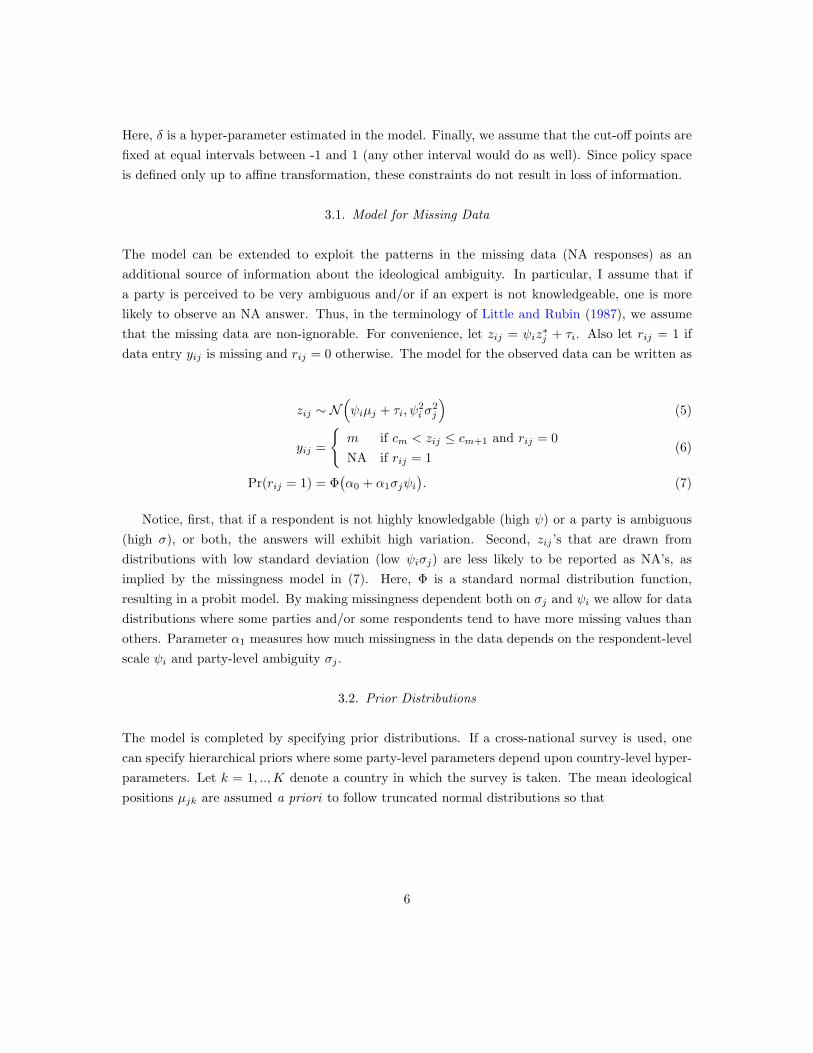
Here, δ is a hyper-parameter estimated in the model. Finally, we assume that the cut-off points arefixed at equal intervals between -1 and 1 (any other interval would do as well). Since policy spaceis defined only up to affine transformation, these constraints do not result in loss of information.

3.1. Model for Missing Data

The model can be extended to exploit the patterns in the missing data (NA responses) as anadditional source of information about the ideological ambiguity. In particular, I assume that ifa party is perceived to be very ambiguous and/or if an expert is not knowledgeable, one is morelikely to observe an NA answer. Thus, in the terminology of Little and Rubin (1987), we assumethat the missing data are non-ignorable. For convenience, let zij = ψiz

∗j + τi. Also let rij = 1 if

data entry yij is missing and rij = 0 otherwise. The model for the observed data can be written as

zij ∼ N(ψiµj + τi, ψ

2i σ

2j

)(5)

yij =

{m if cm < zij ≤ cm+1 and rij = 0NA if rij = 1

(6)

Pr(rij = 1) = Φ(α0 + α1σjψi

). (7)

Notice, first, that if a respondent is not highly knowledgable (high ψ) or a party is ambiguous(high σ), or both, the answers will exhibit high variation. Second, zij ’s that are drawn fromdistributions with low standard deviation (low ψiσj) are less likely to be reported as NA’s, asimplied by the missingness model in (7). Here, Φ is a standard normal distribution function,resulting in a probit model. By making missingness dependent both on σj and ψi we allow for datadistributions where some parties and/or some respondents tend to have more missing values thanothers. Parameter α1 measures how much missingness in the data depends on the respondent-levelscale ψi and party-level ambiguity σj .

3.2. Prior Distributions

The model is completed by specifying prior distributions. If a cross-national survey is used, onecan specify hierarchical priors where some party-level parameters depend upon country-level hyper-parameters. Let k = 1, ..,K denote a country in which the survey is taken. The mean ideologicalpositions µjk are assumed a priori to follow truncated normal distributions so that

6

µjk|δ ∼ N (0, ηµ)1[µjk ∈ (c1 − δ, cM−1 + δ)

](8)

ln(δ) ∼ N (ci+1 − ci, vδ) (9)

We set ηµ = 100 resulting in a vague but proper prior distribution. The hyper-parameter δ isa priori set to have a log-normal distribution with mean equal to the distance between any twocut-off points. We set vδ = 1, resulting in identifiable and yet highly flexible model: under thisspecification, we have 0.44 probability that the most extreme party is two units (one-fifth of thescale) away from the smallest or largest cut-off point. For the remaining parameters, we set

σ2jk|bk ∼ Inv-Gamma(a, (a− 1)bk) (10)

bk ∼ Gamma(ε, ε) (11)

ψik ∼ U(

12 , 2)

(12)

τik ∼ N (0, 1) (13)

In (10), the shape and scale of the inverse gamma distribution is fixed so that the E(σ2jk) = bk.

Setting a = 4 yields a priori variance of b2k/2. Letting ε be a small number (e.g., 0.1), yields a prioron bk with large variance; thus, the priors end up having a negligible effect on the estimates. Thehierarchical priors induce adaptive shrinkage: the estimates of ideological ambiguity in a country kare shrunken towards the common mean bk. The statistical advantages of the hierarchical shrinkageare well-documented in the literature (Gelman et al., 2003).

Further, under priors in (12), each respondent can expand or shrink the perceptual space atmost by a factor of two. Notice that as ψi → 0, the distribution of zij collapses to a degeneratedistribution with the mass at τi. This implies that, for ψi near zero, a respondent would placeall parties on the same point. Similarly, if ψi is very large, a respondent places all parties on theopposite extremes of the scale. Since both of these alternatives are not common, we constraint ψi’sto the specified interval.

Relative to the scale of cut-off points, the prior distribution of τi in (13) also allows sizableidiosyncratic location shifts. Lastly, the selection model parameters α0 and α1 are assumed tofollow normal distributions with 0 mean and variance of 100 (a higher variance reduces the speedof convergence without affecting the results).

7

4. PARAMETER ESTIMATION

The model is estimated using Markov Chain Monte Carlo (MCMC) methods using Gibbs samplingapproach (Gelfand and Smith, 1990). Let Nk and Jk denote the number of respondents and numberof parties in country k respectively. Let Njk denote the set of respondents in country k who haveplaced party j on the scale (Nk − Njk is the number of NA answers for party j in country k).Let y = (yobs,ymis), where yobs is observed and ymis is missing data respectively and let z and rdenote a vector of latent perceptions zijk and missing data indicators rijk respectively. For brevity,let θ denote all parameters of the model. The joint distribution of y, z and r as

π(y, z, r|θ) = π(yobs,ymis, z|r, θ)π(r|θ) (14)

This factorizations yields a pattern-mixture model with shared parameters (Little, 1993). In thismodel, there is a set of common parameters affecting both the distribution of data y and missingnesspattern in r. In the model of missingness given in (7), the distribution of r depends on the vectorsof ambiguity and uncertainty parameters σ and ψ and the coefficient vector α = (α0, α1). Notethat this model differs from selection models of missing data where the distribution of r depends onyobs and ymis but not on the data model parameters. The model for the observed data is derivedby integrating out the missing data from the complete data model, so that

π(yobs, z, r|θ) =∫π(yobs,ymis, z|r,µ,σ, τ ,ψ)π(r|σ,ψ,α)dymis

= π(yobs|r,µ,σ, τ ,ψ)π(r|σ,ψ,α). (15)

This yields the likelihood of the complete data, which is a product of two likelihoods – one forobserved data and one for the model of missing data:

L(y, z, r; θ) ∝K∏k=1

∏i∈Njk

Jk∏j=1

π(yijk, zijk|µjk, τik, σjk, ψik)×

K∏k=1

Nk∏i=1

Jk∏j=1

π(rijk|σjk, ψik,α). (16)

Using previously specified prior distributions, the full conditionals for most of the parametersin the model have known distributional form. Specifically, the Gibbs sampler iterates between thefollowing blocks:

1. Sample latent perceptions zijk conditional on the observed data yijk and all parameters of

8

the model:

zijk|yijk, · ∼ N(µjkψik + τik, ψ

2ikσ

2jk

)1(cyijk

< zijk ≤ cyijk+1)

2. Given the latent variables z, the remaining full conditionals do not depend on the ordinaldata y. The means of the platforms are sampled as follows:

µjk|zjk, · ∼ N(Sjk/Djk, σ

2jk/Djk

)1(c1 − δ < µjk < cM−1 + δ),

where Sjk =∑ik(zijk−τik)/ψik andDjk = Njk+σ2

jk/ηµ. The respondent location parametersare sampled as follows:

τik|· ∼ N

(∑j(zijk − ψikµjk)/σ2

jk∑jk σ

−2jk + ψ2

ik

,ψ2ik∑

jk σ−2jk + ψ2

ik

).

3. Full conditionals for σ and ψ do not have a recognizable form, thus Metropolis-Hastingsalgorithm is employed. The log-posterior of σ2

j is proportional to

lnπ(σ2j |z, µ, τ, ψ, ak, α) ∝− (Njk/2 + 3) lnσ2

jk − σ−2jk (Sjk/2ψ2

ik + bk)

+∑i∈Nk

rijk ln pijk + (1− rijk) ln(1− pijk),

where pijk = Φ(α0 + α1φjkσjk) and Sjk =∑i∈Njk

(zijk − ψikµjk − τik)2. The log-posteriorfor ψ2 has a similar form:

lnπ(ψ2ik|z, µ, σ, τ) ∝− (Jik/2 + 1/2) lnψ2

ik + S1/ψ2ik − S2/ψik

+∑i∈Nk

rijk ln pijk + (1− rijk) ln(1− pijk),

where S1 = .5∑jk(zijk−τik)2σ−2

jk and S2 =∑jk(zijk−τik)µjkσ−2

jk . Proposal values σ2(t)jk are

sampled from the inverse gamma with shape λ and scale (λ− 1)σ2(t−1)jk ; that is, the proposal

value is drawn from the distribution centered around the previous value of the sample. Here,λ is the tuning parameter that set to to achieve an acceptance rate between 30 and 50%.

4. ln(δ) is sampled from the left-truncated normal distribution with mean ci+1−ci, unit varianceand lower bound equal to ln(max{µjk} − cM−1). The conditional distribution for the hyper-parameter bk is gamma with scale 2Jk + ε and rate (a− 1)

∑j σ−2j + 1/ε.

5. The coefficients in the missing data model, α0 and α1, are sampled using the standard dataaugmentation method by Albert and Chib (1993).

9

To implement the identification constraints in equation 4, after each block of iterations, eachψik is divided by the country average of ψik’s; similarly, from each τik the country average of τik’sis subtracted. This procedure is similar to hierarchical centering by “sweeping” and is known toimprove the convergence of MCMC algorithms in weakly identified models (Robert and Casella,2004, p. 397). The convergence can be monitored using the standard tools, as, for example, Geweke(1992) or Heidelberger and Welch (1983) diagnostics.

5. APPLICATION: IDEOLOGICAL AMBIGUITY AND ELECTORAL PERFORMANCE

We apply our model to the expert data collected by Benoit and Laver (2006). The survey wasconducted in 48 countries with about 8 parties and 30 experts per country on average. The analyzeddataset contains 10,603 entries with about 9% of missing values, 364 parties, and 1493 experts. Ourgoal is to investigate whether a party’s ambiguity on the issue of taxation and provision of publicservices is related to its ideological extremism and vote-share in the last elections.

In the survey, the experts were asked to place political parties on the 20 point scale with theend-points defined as follows:

[1] Party promotes raising taxes to increase public services.

[20] Party promotes cutting public services to cut taxes.

The posterior estimates of σ are very different from the naive sample standard deviation, withcorrelation of only 36 percent. The posterior mean of the missing data mechanism parameter α1

is 0.245 with the standard deviation of 0.014 indicating that the missingness of the data is relatedto the ambiguity of party positions and the uncertainty of experts. Together this serves as theevidence that (1) the sample standard deviation would yield an incorrect measure of ideologicalambiguity if the assumed model is valid and that (2) the patterns in missing data do provideadditional information about the ideological ambiguity and respondent uncertainty.

Using direct measures of ideological ambiguity and voters’ uncertainty, the previous literaturehas found that ambiguity is related to voting behavior (Alvarez, 1997; Tomz and van Houweling,2009). Therefore, ideological ambiguity should also be also related to a party’s electoral perfor-mance. In case the model provides correct estimates of ideological ambiguity, one should observea relationship between the posterior estimates of ideological ambiguity and vote-shares of politicalparties. Furthermore, if the sample standard deviation σ is not a valid measure of ideological am-biguity (as was suggested earlier), the association between σ and the parties’ electoral performanceshould be low.

After computing the posterior distributions of σjk’s for all parties in the dataset, the followingmodel was estimated:

10

T (vjk) = β0 + β1|µjk − µ|+ β21

1 + σjk+ εjk, (17)

where vjk is a vote-share of party j in country k, T (·) is a Box-Cox transformation, and µ is theestimated empirical center of party platforms. The coefficients β1 and β2 represent the effect of ide-ological extremism and ideological precision (the inverse of the ideological ambiguity) respectively.

The model in (17) was estimated in three settings. In the first setting, I used the sample meanµ and standard deviation σ in place of µ and σ in equation 17. In the second setting, the meanposterior estimates E(µ|y) and E(σ|y) derived from the latent hierarchical model were used in placeof µ and σ. Both of the above models do not take into account the fact that the covariates (µ, σ)and (E(µ|y),E(σ|y)) are only estimates that are measured with error, not fixed values. Ignoring,the presence of the measurement error in the covariates might lead to invalid inference about theregression parameters in model (17).

Therefore, in the third setting, the linear regression with measurement error was fit to the data.This is accomplished easily by adding a step in the Gibbs sampling algorithm. Assuming uniformpriors over the coefficients β and regression error s2 – π(β, s2) ∝ 1/s2 – one can sample β from themultivariate normal distribution with mean (X ′X)−1X ′T (v) and covariance matrix s2(X ′X)−1,where X is the design matrix for model in (17) and v is the vector of vote-shares. At each iteration,the columns of X representing µ and σ are replaced with a draw from the posterior π(µ|y) andπ(σ|y) respectively. Finally, s2 is sampled from the inverse gamma distribution with shape J/2(where J is the overall number of parties in the analysis) and scale (T (v)−X′β)′(T (v)−X′β)/2.

Results of the three analyses are reported in Table 2. First, let us compare the two frequentistsregressions that use the naive sample estimates and the average posterior estimates from the pro-posed model. Evidently, there are stark differences: If the sample estimates of µ and σ are used,there is no statistically tractable relationship between the electoral performance of a party and itsideological ambiguity or extremism. None of the coefficients are significant at conventional levelsand the overall fit of the model is extremely poor, with both R2 and F -statistic being extremelylow. Both of these results are counter-intuitive as existing theories and evidence would suggestthat ideological extremism is rarely rewarded by voters and that ideological ambiguity does affectvoters’ behavior.

In contrast, if one uses the measures of µ and σ derived from the proposed latent hierarchicalmodel, the model fit increases dramatically as indicated by lower root mean squared error (RMSE),higher R2 and F -statistic and substantially lower Aikaike’s Information Criterion (AIC). In thismodel, increasing ideological ambiguity and extremism are both statistically associated with worseelectoral performance. Since this empirical pattern is closer to the theoretical expectations, thissuggests that the measure σ derived from the latent hierarchical model does improve upon the naiveestimator.

11

Table 2: Ideological ambiguity and electoral performance of parties.

No Measurement Errora With Measurement Errorb

µ, σ E(µ|y),E(σ|y) E(µ|y),E(σ|y)Intercept -2.32∗∗ -3.125∗∗∗ -3.823c

(0.115) (0.156) [ -4.393, -3.275]d

Extremism: -0.01 -0.073∗ -0.049|µjk − µ| (0.03) (0.042) [-0.137, 0.030]

Ideological precision: 0.039 2.875∗∗∗ 3.8601/(1 + σjk) (0.612) (0.413) [2.486, 5.126]

RMSE 1.126 1.057R2 0.1-e4 0.12AIC 1124 1078F (2, 361) 0.062 24.5N 364 364

∗p < 0.1, ∗∗∗p < 0.001.a Frequentist regression ignoring the measurement error in the covariates. Standard

errors in the parentheses.b Bayesian regression with flat priors accounting for the measurement error.c Posterior mean.d 95% highest posterior density interval.

Finally, the third model which takes into account the measurement error in µ and σ, showsqualitatively similar results, albeit, with some important deviations. First, the effect of ideologicalextremism is now lower and the 95% credible now covers zero (though 90% credible interval doesnot cover zero, however). Second, the effect of ideological precision increases by about 1/3 whenthe measurement error is taken into account. Fitting the model with the measurement error is moreappropriate given the nature of the problem and it is advisable to use this approach as a standardpractice.

It is important to note that we do not claim to have found any causal effect of ideologicalambiguity on the electoral performance. It might well be the case that smaller political partieshave fewer means to communicate their policy positions and there is nothing in the design of ouranalysis that would allow us to circumvent this problem. Instead, the nature of this exercise wasmerely to show that these two quantities are associated – as we should expect them to be – andthat the sample estimates of ideological ambiguity would (perhaps erroneously) lead us to believethat they are not.

6. DISCUSSION

The goal of this study was to construct and evaluate a model that allows to estimate ideologicalambiguity from survey data. The proposed model focused on synthesizing two distinct approaches

12

previously used by political methodologists – one approach focused on disagreement among therespondents while another approach attempted to infer the degree of ideological ambiguity fromthe patterns of missing data. This study demonstrated how these two approaches can be synthe-sized into a single inferential framework yielding more accurate and more informative measures ofideological ambiguity than what is offered by focusing on naive sample standard deviations. Thegreater accuracy results from the fact that the latent hierarchical model exploits the rich informa-tional structure of the survey data and allows to represent policy positions of parties in terms ofprobability distributions rather than points.

Although the proposed method of inferring ideological ambiguity is promising, there are severalissues that should be further studied. First, the model relies heavily on the assumption that thepatterns of data missingness are related to underlying ideological ambiguity. The estimates of themodel will be biased to the extent that this assumption is violated. A survey experiment where,in placing parties, some respondents can using the interval scales (e.g. Tomz and van Houweling,2009) while others must place them on the standard single-point scales could evaluate the empir-ical plausibility of this assumption. Second, external validation analyses using direct measures ofideological ambiguity as benchmarks could also elicit potential strengths and weaknesses of theproposed model.

REFERENCES

Albert, James H. and Siddgartha Chib. 1993. “Bayesian Analysis of Binary and PolychotomousResponse Data.” Journal of American Statistical Association 88(442):669–679.

Aldrich, John. 1983. “A spatial model with party activists: implications for electoral dynamics.”Public Choice 41(1):63–100.

Aldrich, John. 1995. Why Parties?: The Origin and Transformation of Political Parties in America.University of Chicago Press.

Aldrich, John and Richard Mckelvey. 1977. “A Method of Scaling with Applications to the 1968and 1972 Presidential Elections.” American Political Science Review 71(1):111–130.

Alesina, Alberto and Alex Cukierman. 1990. “The Politics of Ambiguity.” The Quarterly Journalof Economics 105(4):829–850.

Alvarez, Michael R. 1997. Information and Elections. University of Michigan Press.

Ansolabehere, S., J.M. Snyder Jr and C. Stewart III. 2001. “Candidate positioning in US Houseelections.” American Journal of Political Science 45(1):136–159.

Bartels, Larry. 1986. “Issue Voting Under Uncertainty: An Empirical Test.” American Journal ofPolitical Science 30:709–728.

Benoit, Kenneth and Michael Laver. 2006. Party Policy in Modern Democracies. London: Rout-ledge.

13

Callander, Steven and Catherine H. Wilson. 2008. “Context-dependent Voting and Political Am-biguity.” Journal of Public Economics 92(3-4):565 – 581.

Campbell, James E. 1983a. “Ambiguity in the Issue Positions of Presidential Candidates: A CausalAnalysis.” American Journal of Political Science 27(2):284–93.

Campbell, James E. 1983b. “The Electoral Consequences of Issue Ambiguity: An Examination ofthe Presidential Candidates’ Issue Positions from 1968 to 1980.” Political Behavior 5(3):277–91.

Clinton, Joshua D. and David E. Lewis. 2007. “Expert Opinion, Agency Characteristics, andAgency Preferences.” Political Analysis 16(1):3–20.

Clinton, Joshua D. and Douglas Jackman, Simon a dn Rivers. 2004. “The Statistical Analysis ofRoll Call Data.” American Political Science Review 98:355–370.

Evans, Geoffrey and Stephen Whitefield. 2000. Explaining the Formation of Electoral Cleavages inPost-Communist Democracies. In Elections in Central and Eastern Europe. The First Wave, ed.H.D. Klingemann. Berlin: Edition Sigma.

Gelfand, Allan E. and Adrian F. M. Smith. 1990. “Sampling-Based Approaches to CalculatingMarginal Densities.” Journal of the American statistical association 85(410):398–409.

Gelman, Andrew, John B. Carlin, Hal B. Stern and Donald B. Rubin. 2003. Bayesian Data Analysis.2 ed. Chapman and Hall.

Geweke, John. 1992. Evaluating the Accuracy of Sampling-based Approaches to Calculating Pos-terior Moments. In Bayesian Statistics 4, ed. J.M Bernado, J.O. Berger, A.P Dawid and AdrianF. M. Smith. Clarendon Press, Oxford.

Glazer, Amihai. 1990. “The Strategy of Candidate Ambiguity.” The American Political ScienceReview 84(1):237–41.

Heidelberger, Philip and Peter D. Welch. 1983. “Simulation Run Length Control in the Presenceof an Initial Transient.” Operations Research 31:1109–44.

Huyse, Luc and Ben H. Thacker. 2004. Decision Making under Uncertainty on the Basis of ExpertOpinion. In Manuscript.

Johnson, Valen E. and James H. Albert. 1999. Ordinal Data Modeling. Springer.

Kitschelt, H., Zdenka Mansfeldova, Radoslaw Markowski and Gabor Toka. 1999. Post-CommunistParty Systems. Cambridge: Cambridge University Press.

Laver, M., K. Benoit and J. Garry. 2003. “Extracting policy positions from political texts usingwords as data.” American Political Science Review 97(2):311–331.

Little, Roderick J. A. 1993. “Pattern-Mixture Models for Multivariate Incomplete Data.” Journalof American Statistical Association 88(421):125–134.

Little, Roderick J. A. and Donald Rubin. 1987. Statistical Analysis With Missing Data. John Wiley& Sons.

14

Mainwaring, Scott. 1995. Brazil: Weak Parties, Feckless Democracy. In Building Democratic Insti-tutions, ed. Scott Mainwaring and Timothy Scully. Stanford University Press.

Marks, Gary, Liesbet Hooghe, Marco R. Steenbergen and Ryan Bakker. 2007. “CrossvalidatingData on Party Positioning on European Integration.” Electoral Studies 26(1):23–38.

Martin, Andrew D. and Kevin M. Quinn. 2002. “Dynamic Ideal Point Estimation via Markov ChainMonte Carlo for the U.S. Supreme Court, 1953–1999.” Political Analysis 10(2):134–153.

Miller, Gary and Norman Schofield. 2003. “Activists and Partisan Realignment in the UnitedStates.” American Political Science Review 97(2):245–60.

Page, Benjamin I. 1976. “The Theory of Political Ambiguity.” The American Political ScienceReview 70(3):742–52.

Palfrey, Thomas R. and Keith T. Poole. 1987. “The Relationship between Information, Ideology,and Voting Behavior.” American Political Science Review 31(3):511–539.

Robert, Christian P. and George Casella. 2004. Monte Carlo Statistical Methods. 2 ed. Springer.

Scully, Timothy. 1995. Reconstituting Party Politics in Chile. In Building Democratic Institutions,ed. Scott Mainwaring and Timothy Scully. Stanford University Press.

Shepsle, Kenneth A. 1972. “The Strategy of Ambiguity: Uncertainty and Electoral Competition.”The American Political Science Review 66(2):555–68.

Tomz, Michael and Robert P. van Houweling. 2009. “The Electoral Implications of CandidateAmbiguity.” American Political Science Review 103(1):83–98.

Zaslavsky, Alan. 2003. Hierarchical Bayesian Modeling. In Subjective and Objective Bayesian Statis-tics. Principles, Models, and Applications, ed. James S. Press. Wiley.

15

Biographies

1 Editors�Biographies

Norman Scho�eld was the Director of the Center in Political Economy atWashington University in Saint Louis from 1992 until 2012, He is currently theWilliam R. Taussig Professor of Political Economy, and Professor in the Depart-ments of Economics and Political Science . He has PhD�s in both governmentand economics from Essex University, a LittD from Liverpool University and adoctorat d�etat from the University of Caen. He is currently working on top-ics in the theory of social choice, political economy, and democracy. He haswritten several books, including Multiparty Government (with Michael Laver,in 1990), Social Choice and Democracy (Springer,1985), and edited or co-editedten volumes, including The Political Economy of Institutions, Democracy andVoting, (Co-edited with Gonzalo Caballero, Spinger, 2011). His book, Mathe-matical Methods in Economics and Social Choice, was published by Springer in2003. In 2006 he published Architects of Political Change as well as MultipartyDemocracy (with Itai Sened) both with Cambridge University Press. His book,The Spatial Model of Politics was published by Routledge in 2008, followed byThe Political Economy of Democracy and Tyranny in 2009 with Oldenbourg(Munich). He has just completed a book, Leadership or Chaos (co-authoredwith Maria Gallego, published by Springer in 2011). He has been the recipientof a number of NSF awards, most recently one on electoral politics and regimechange. In 2003 he was the Fulbright distinguished professor at Humboldt Uni-versity and ,in 2007 and 2008, visiting fellow at ICER in Turin. In Spring 2008he was the visiting Leitner Professor at Yale University and was a NationalFellow at the Hoover Institution in summers 2009 and 2010. He was recipientof the Riker prize for contributions to political theory in 2002, and was electedto the American Academy of Arts and Sciences in 2005.<scho�eld.norman@gmail.com>Gonzalo Caballero is an Associate Professor of Economics at the Uni-

versity of Vigo, Spain. He received his PhD and a B.Sc. in Economics withHonors from the University of Vigo, and he received a MPhil in Contempora-neous Political Studies from the University of Santiago de Compostela.He hasbeen a Visiting Scholar at the Center for New Institutional Social Sciences,Washington University in St. Louis, the Center for Advanced Study in the So-cial Sciences in Madrid, the University of California in Santa Barbara and theUniversity of California in Berkeley. He taught a course on �Economics of Insti-tutions�at Charles University in Prague, at Comenius University in Bratislavaand at the University Roma Tre. He has published many papers on institu-tional analysis in various journals, including Economic Modelling, Journal ofInstitutional Economics, Ocean & Coastal Management, Marine Policy, Envi-ronmetrics, El Trimestre Económico, Brazilian Journal of Political Economy,Política y Gobierno, Revista Española de Investigaciones Sociológicas, Revistade Estudios Políticos and Revista Española de Ciencia Política. He has written

1

several books and co-edited a volume on the Great Recession.<gcaballerom@yahoo.com>Daniel Kselman is a Research Fellow at the Center for Advanced Studies in

the Social Sciences, Juan March Institute (Madrid). His research employs bothgame theoretic and econometric modelling to study the impact if political insti-tutions and political party organizations on a variety of contemporary politicalphenomena, including but not limited political corruption, legislative instability,and democratic accountability. He is also a student of modern Turkish politics,and has written on Turkish political institutions and party organizations.<dkselman@march.es>

2 Biographies of Contributors

James Adams is Professor of Political Science at the University of Californiaat Davis. He studies voting behavior, parties�election strategies, and politicalrepresentation in Western Europe and the UnitedStates. His research, whichencompasses both spatial models of party competition and empirical analysesof parties�policy programmes, has appeared in the American Political ScienceReview, the American Journal of Political Science, the Journal of Politics, Po-litical Analysis, and Public Choice.<jfadams@ucdavis.edu>Luz Marina Arias received her Ph.D. in Economics from Stanford Uni-

versity. Her research focuses on the political economy of economic and politicaldevelopment, and in particular on the mechanisms behind institutional changeand continuity. Her work has centered on the indigenous origins of colonial laborin the Americas, and on the origins of centralized �scal capacity in Latin Amer-ica. She has received fellowship positions from the Center for U.S.-MexicanStudies at the University of California in San Diego and the Center on Democ-racy, Development and the Rule of Law at Stanford University. Luz Marinawas born and raised in Mexico City and completed her undergraduate studiesin Economics at ITAM, Mexico City.<larias@march.es>,Xosé Carlos Arias is Professor of Economics and Economic Policy at the

University of Vigo (Spain). In recent years, he actively worked in the analysisof the �nancial crisis in the world economy and the development of the researchprogram of Transaction Cost Politics. He recently published the book La torrede la arrogancia. Políticas y mercados después de la tormenta, (Ariel, Barcelona,2011), jointly with Antón Costas. He also co-edited Organización de gobiernosy mercados, (PUV, Valencia). He has published several papers on di¤erenttopics in journals such as Desarrollo Económico, Revista de Economía Aplicada,Revista Española de Ciencia Política and Revista de Economía Institucional,among others.<xcarias@uvigo.es>Thomas L. Brunell is a professor of Political Science at the University of

Texas at Dallas. His teaching and research interests revolve around elections,

2

representation, political parties and the U.S. Congress. He received his Ph.D.from the University of California, Irvine in 1997. His book Representation andRedistricting: Why Competitive Elections are Bad for America" was publishedin 2008,. He is currently working on a book about partisan gerrymandering.<tlb056000@utdallas.edu>Ernesto Calvo (PhD Northwestern) is an Associate Professor of Political

Science at the University of Maryland. His research focuses on issues of polit-ical representation, elections and Congresses. His research, which has receivedawards from the Representation and the Comparative Politics sections of theAmerican Political Science Association, has been published in US, European,and Latin American journals such as the American Journal of Political Science,the Journal of Politics,World Politics, The British Journal of Political Science,Comparative Political Studies, Electoral Studies, Política y Gobierno (Mexico),Desarrollo Económico (Argentina), Opiniao Publica (Brazil), and the Revistade Ciencia Politica (Chile).<ecalvo@umd.edu>Kiyoung Chang is a Ph.D. Student in Government and Politics at the

University of Maryland. His research interests include the di¤usion of terrorism,bargaining in civil war, domestic audience costs, and U.N. voting.<Kiyoung Chang@gmail.com>Harold D. Clarke, (Ph.D. Duke University) is Ashbel Smith Professor,

School of Economic, Political and Policy Sciences, University of Texas at Dal-las, and Adjunct Professor, Department of Government, University of Essex.He also is editor of Electoral Studies. Clarke�s research on electoral choice andthe political economy of party support in Great Britain, the United States andCanada has been supported by the National Science Foundation (U.S.), theEconomics and Social Research Council (U.K.), and the Social Sciences andHumanities Research Council (Canada). He is currently a principal investigatorfor the 2009/10 British Election Study and the 2008 Political Support in Amer-ica Study. Other current research projects include the 2009 Political Supportin Germany Study, and the 2008 Political Support in Canada Study. He is theauthor of numerous articles published in journals such as the American Journalof Political Science, the American Political Science Review, the British Journalof Political Science, the Journal of Politics and Political Analysis. His mostrecent books are Performance Politics and the British Voter (Cambridge: Cam-bridge University Press, 2009), Making Political Choices: Voting in Canada andthe United States (Toronto: University of Toronto Press), and Political Choicein Britain (Oxford: Oxford University Press, 2004). Clarke�s teaching interestsfocus on public opinion, voting and elections and research methods. He regu-larly teaches advanced time series analysis at the Essex Summer School in DataCollection and Analysis and the Concordia University Spring School.<hclarke@utdallas.edu>Betul Demirkaya is a graduate student in political science at Washington

University in Saint Louis.<betul.demirkaya@wustl.edu>Leandro De Magalhaes studied Economics at the University of Brasilia

and received his PhD from Bocconi University. For two years during his PhD

3

he was a visiting student at the University of Pennsylvania. He is currently anAssistant Professor at Bristol University. He has worked on the size of govern-ment in the American states, on Brazilian politics, and is currently working onwar �nancing and political transitions.<leandro.magalhaes@bristol.ac.uk>Jon X. Eguia is an assistant professor in the Department of Politics and

a¢ liated to the Department of Economics at New York University. He obtainedhis PhD from the California Institute of Technology in 2007. His �elds of spe-cialization are political economy, formal political theory, social choice and publiceconomics. His work on party formation, voting and elections, and the spatialmodel of policy preferences has been published in leading political science jour-nals such as the American Journal of Political Science and theQuarterly Journalof Political Science and in economic theory journals such as Social Choice andWelfare , Games and Economic Behavior, Economic Theory and the Journalof Mathematical Economics among others.<equia@nyu.edu>Bernard Grofman is the Jack W Peltason (Bren Foundation) Endowed

Chair at University of California at Irvine(UCI), and Professor of Political Sci-ence and Director of the UCI Center for the Study of Democracy His researchdeals with topics such as voting rights and theories of representation and elec-toral rules. He is co-author of 4 books (published by Cambridge UniversityPress), and co-editor of 21 other books; with 250 research single and co-authoredarticles and book chapters, including ten in the American Political Science Re-view. He has been a visiting faculty member at nearly a dozen universities inthe U.S. and Europe. He is a Fellow of the American Academy of Arts and Sci-ences, and has an Honorary Doctorate in Political Science from the Universityof Copenhagen.<bgrofman@uci.edu>Timothy Hellwig is an associate professor of political science at Indiana

University. His research interests focus on the political economy of advancedindustrial societies. He is currently completing a book manuscript on economicglobalization and electoral politics. His work on globalization, economic vot-ing, and party politics appears in the American Journal of Political Science,The British Journal of Political Science, The Journal of Politics, among otheroutlets.<thellwig@indiana.edu>JeeSeong Jeon is a graduate student in political science, at Washington

University in Saint Louis. She has published papers in the Journal of Elections,Public Opinion and Politics, and Electoral Studies.<jsjeon@wustl.edu>Dean Lacy is Professor of Government and Director of the Program in

Politics and Law at Dartmouth College. His Ph.D. in Political Science is fromDuke University.<Dean.P.Lacy@dartmouth.edu>Kevin McCalister is a graduate student in political science, at Washington

University in Saint Louis.

4

<kevinmcalister@wustl.edu>Samuel Merrill, III. is Professor Emeritus of Mathematics and Computer

Science at Wilkes University. He received his Ph.D. in mathematics from YaleUniversity. His current research involves mathematical and statistical model-ing, particularly in political science. He is the author of A Uni�ed Theory ofParty Competition (Cambridge University Press 2005; with James Adams andBernard Grofman), A Uni�ed Theory of Voting (Cambridge University Press2005; with Bernard Grofman), and Making Multicandidate Elections More De-mocratic (Princeton University Press 1988). He has published in a number ofjournals, including the American Political Science Review, the American Jour-nal of Political Science, and the British Journal of Political Science. He has beena Visiting Professor at Yale University and a visiting scholar at the Universityof Washington.<sammerrill3@comcast.net>Katja Michalak is reader of political science and public administration at

the Department of Public Management and Governance at Zeppelin University.She holds a Master�s degree in political science with a focus on democratizationin Eastern Europe and a Master�s degree in psychology with a focus on politicalpsychology and organizational psychology. She received her doctorate (PhD)in the �eld of �Comparative Institutions� from Ohio State University with athesis on �Civil Service Reform and the Quality of Governance in Eastern Eu-rope�. Her research interests include comparative politics, political governance,bureaucracy, political institutions, democratization, and political psychology.< katja.michalak@zu.de>Emerson Niou (Ph.D., U. of Texas at Austin, 1987), Professor of Po-

litical Science, specializes in Formal Theory, International Relations, PoliticalEconomy, and East Asian Politics. He is the co-author of The Balance of Power,(Cambridge University Press, 1989). His publications in the �eld of internationalrelations include: "Less Filling, Tastes Great: The Realist-Neoliberal Debate,"coauthored with P. C. Ordeshook, World Politics, January 1994 and "Alliancesin Anarchic International Systems," coauthored with P. C. Ordeshook, Inter-national Studies Quarterly, June 1994. In the �eld of East Asian politics, hisrecent publications include: "An Analysis of Dr. Sun Yet-sen�s Self-AssessmentScheme for Land Policy," with G. Tan, Public Choice, December 1993; "SeatBonuses under the Single Non-Transferable Vote for Large Parties: Evidencefrom Japan and Taiwan," with G. Cox, Comparative Politics, January 1994;and "Police Patrol vs. Self-Policing: A Comparative Analysis of the ControlSystems Used in the Ex-Soviet Union and the Communist China," with JohnBrehm, Journal of Theoretical Politics, 1996. His current projects include stud-ies of local self-government in China and alliance politics in anarchic interna-tional systems. Professor Niou is Director of the Program in Asian SecurityStudies at Duke University.<niou@duke.edu>John Patty is a formal political theorist whose research focuses on political

institutions. He regularly teaches undergraduate courses on Congress and thefederal bureaucracy as well as graduate courses on game theory and formal mod-

5

els of political institutions, at Washington University in Saint Louis. His workhas been published in American Journal of Political Science, Annual Review ofPolitical Science, Economics & Politics, Electoral Studies, Games & EconomicBehavior, Journal of Politics, Journal of Theoretical Politics, Mathematical &Computer Modelling, Politics, Philosophy, & Economics, Public Choice, Quar-terly Journal of Political Science, and Social Choice & Welfare. In additionto serving as an Associate Editor of the American Journal of Political Science,he currently serves on the editorial boards of Political Analysis and Journal ofTheoretical Politics. He received his Ph.D. in Social Sciences from the CaliforniaInstitute of Technology in 2001. Prior to coming to Washington University, hewas Assistant Professor of Political Economy and Decision Sciences at CarnegieMellon University and Assistant Professor of Government at Harvard University.His book Learning While Governing: Expertise and Accountability in the Exec-utive Branch (with Sean Gaillmard) will appear with the University of ChicagoPress in 2013<jwpatty@gmail.com>Gerald Pech is associate professor of economics at KIMEP University. He

received his PhD from Ruhr-University Bochum in Germany in 1995. Since thenhe hasheld teaching and research positions at the Graduate School Bochum andDortmund, the University of St Andrews, the National University of Irelandin Galway, the American University in Bulgaria and the University of Mainz.His areas of research are collective decision making and economic and politicalinstitutions.<gp@geraldpech.net>Elizabeth Maggie Penn is a formal political theorist whose work focuses

on social choice theory and political institutions. She regularly teaches un-dergraduate courses on electoral systems and agent-based modeling as wellas graduate courses on positive political theory, at Washington University inSaint Louis. Her work has been published in the American Journal of PoliticalScience, Journal of Politics, Journal of Theoretical Politics, Mathematical &Computer Modelling, Public Choice, Social Choice & Welfare, and Complexity.Professor Penn received her Ph.D. in Social Sciences from the California Insti-tute of Technology in 2003 and her B.A. from the University of California atBerkeley in 1999. Previously, she was Assistant Professor of Political Economyand Decision Sciences at Carnegie Mellon University (2003-2005) and AssistantProfessor of Government at Harvard University (2005-2009).<elizabeth.m.penn@gmail.com>Arturas Rozenas holds Ph.D. in Political Science and M.S. in Statistical

and Decision Sciences, both from Duke University. His research focuses on game-theoretic and statistical models of democratic and non-democratic elections andBayesian statistics. Currently, he is teaching at the ISM University of Manage-ment and Economics in Vilnius, Lithuania. In the fall of 2013, he will be joiningthe Department of Politics at New York University. <arturasro@gmail.com>David Sanders, is a Professor of Government and Pro-Vice-Chancellor

(Research) at the University of Essex, where he has taught politics since 1975.He is author of numerous books and articles on various aspects of UK and com-

6

parative politics. He has been a Fellow of the British Academy since 2005, andwas joint editor of the British Journal of Political Science from 1990 to 2008.Heis the author of Patterns of Political Instability (1981); Lawmaking and Co-operation in International Politics (1986); Losing an Empire; Finding a Role:British Foreign Policy Since 1945 (1990), and co-author of On Message (1998);Political Choice in Britain (2004); Performance Politics (2009). His currentresearch is on the British Election Study, as well as political participation; elec-tion forecasting; the politics of the UK public sector; measuring and assessingEuropean citizenship.<sanders@essex.ac.uk>Keith.schnakenberg is a PhD student in political science at Washington

University in Saint Louis<keith.schnakenberg@gmail.com>Evan Schnidman obtained his AB and AM in political economy from

Washington University in Saint Louis. He is currently a graduate student in theDepartment of Government, Harvard University.<evan.schnidman@gmail.com>Gilles Serra graduated with a PhD in Political Economy and Govern-

ment from Harvard University in 2007. He won a fellowship to do post-doctoralresearch at Nu¢ eld College at the University of Oxford until 2010, and he is cur-rently an assistant professor at the Center for Economics Research and Teaching(CIDE) in Mexico City. Dr. Serra uses formal theory to study political parties,elections, campaigns, and congressional reforms. His main regions of interestare Latin America and the United States. His publications have appeared inrespected academic journals such as the Journal of Politics, the Journal of The-oretical Politics, and Política y Gobierno. This research has been presented inseveral universities in the United States, Europe, Latin America and Canada.<gilles.serra@cide.edu>Olga Shvetsova is an associate professor of political science and economics

at Binghamton University, USA. She studies political mechanisms as they areshaped by institutional choices. Her long-term research focus is on incentives topolitical elites and how those can lead to amelioration of societal con�ict. Shepublishes in the �elds of political economy of federalism and determinants ofparty system stability and change in democracies. She co-authored DesigningFederalism: A Theory of Self-Sustainable Federal Institutions (with MikhailFilippov and Peter C. Ordeshook, Cambridge University Press,2004) and is nowworking on Parties and Party System Change in Legislatures Worldwide (withCarol Mershon).<shvetsova@gmail.com>Katri Sieberg is the Erkko Professor of North American Studies in the

School of Social Sciences and Humanities at the University of Tampere in Fin-land. Her research combines approaches from economics and political scienceto address the issues of how and why things work - or don�t work. To that end,her research uses social choice theory to address how people make decisions,policy analysis to assess the e¤ect of these decisions, and experimental analysisto evaluate the underlying theories. One of her key interests is welfare state

7

institutions, with a recent focus on health care structures.<katri.sieberg@uta.�>Marianne C. Stewart (Ph.D. Political Science, Duke University), is a Pro-

fessor, and Co-Director of The Survey Center for Opinion Research and Elec-tions, in the School of Economic, Political and Policy Sciences at the Universityof Texas at Dallas. She also has been Executive Vice-Dean, Acting Dean, Grad-uate Studies Director, and Political Science Program Director in the School atUTD, and on the faculties of Virginia Polytechnic Institute and State Univer-sity and Rutgers University. She has been Editor of The American Journal ofPolitical Science, Associate Editor of International Studies Quarterly, AssistantEditor of The Journal of Politics, and Political Science Program Director in theDivision of Social and Economic Sciences of the National Science Foundation.She conducts research and teaches in the areas of electoral politics, polit-

ical behavior, and research methodology. She has been co-investigator of theBritish Election Study (2001, 2005, 2009-10), and funded by the National Sci-ence Foundation and the Economic and Social Research Council (U.K.). Herarticles have been published in The American Journal of Political Science, TheAmerican Political Science Review, The British Journal of Political Science,The Journal of Politics, Political Analysis, and other major research journals.Her recent books are Political Choice in Britain (Oxford University Press, 2004)and Performance Politics and the British Voter (Cambridge University Press,2009).<mstewart@utdallas.edu>Fernando Toboso is Senior Lecturer at the Department of Applied Eco-

nomics, University of Valencia, Spain. His research interests are in methodologi-cal and epistemological issues in economic analysis as well as the organization ofpolicy tasks and public services provision, with an emphasis on the new Spanishfederalism. He has contributed to several edited volumes on these topics andhas published in various academic journals including the Cambridge Journal ofEconomics, Regional and Federal Studies, European Journal of Law and Eco-nomics, Journal of Interdisciplinary Economics, Hacienda Pública Española, ElTrimestre Económico, and Presupuesto y Gasto Público. He has been a visitingscholar at the Public Choice Center, George Mason University, Leeds University,and the University of Bologna, Italy. He has also served as invited editor and au-thor for a special issue published in the Chilean Revista de Análisis Económico,and has recently co-edited a book on economics and institutions.<Fernando.Toboso@uv.es>22. Paul Whitely is the author of The Labour Party in Crisis; Political

Control of the Macroeconomy. and Co-author of Advanced Statistical Methodsin the Social Sciences; Pressure for the Poor - The Poverty Lobby and Policy-Making; How Voters Change: The 1987 British General Election Campaign inPerspective; Controversies in Political Economy - Canada, Great Britain andthe United States; Labour�sGrassroots - The Politics of Party Membership; TrueBlues: The Politics of Conservative Party Membership; High Intensity Partici-pation - The Dynamics of the Party Activism in Britain; New Labour�s Grass-roots: The Transformation of the Labour Party Membership; Political Choice

8

in Britain: Citizenship in Britain: Values, Participation and Democracy; ThirdForce Politics: Liberal Democrats at the Grassroots; Performance Politics andthe British Voter. Author or co-author of more than �fty articles on: politicaleconomy; electoral behaviour; political parties; British politics, citizenship, so-cial capital and quantitative methods in political science. He was Director of theEconomic and Social Research Council Research Programme on Democracy andParticipation, 1998-2003 and co-director of the ESRC funded British ElectionStudy.<whiteley@essex.ac.uk>

9