advanced signal processing lecture 1: random …mandic/asp_slides/asp_lecture_1_slides... ·...

Advanced Signal Processing

Lecture 1: Random Variables

Prof Danilo Mandic

room 813, ext: 46271

Department of Electrical and Electronic Engineering

Imperial College London, [email protected], URL: www.commsp.ee.ic.ac.uk/∼mandic

c© D. P. Mandic Advanced Signal Processing 1

Introduction Recap

Discrete Random Signals:

discrete vs. digital # quantisation

◦ {x[n]}n=0:N−1 is a sequence of indexed random variablesx[0], x[1], . . . , x[N − 1], and the symbol ′[·]′ indicates the randomnature of signal x every sample is random too!

◦ The sequence is discrete with respect to sample index n, which can beeither the standard discrete time or some other physical variable, suchas the spatial index in arrays of sensors

◦ A random signal x[n] can be real or complex

NB: signals can be continuous or discrete in time as well as amplitude

Digital signal = discrete in time and amplitude

Discrete–time signal = discrete in time, amplitude either discrete or continuous


Standardisation and normalisation(e.g. to be invariant of amplifier gain or the quality of sensor contact)

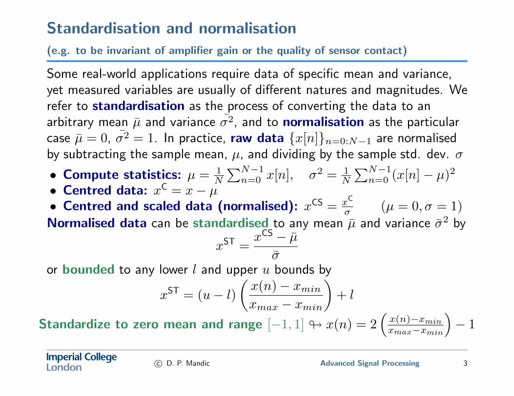
Some real-world applications require data of specific mean and variance,yet measured variables are usually of different natures and magnitudes. Werefer to standardisation as the process of converting the data to anarbitrary mean µ and variance σ2, and to normalisation as the particularcase µ = 0, σ2 = 1. In practice, raw data {x[n]}n=0:N−1 are normalisedby subtracting the sample mean, µ, and dividing by the sample std. dev. σ

• Compute statistics: µ = 1N

∑N−1n=0 x[n], σ2 = 1

N

∑N−1n=0 (x[n]− µ)2

• Centred data: xC = x− µ• Centred and scaled data (normalised): xCS = xC

σ (µ = 0, σ = 1)

Normalised data can be standardised to any mean µ and variance σ2 by

xST =xCS − µ

σor bounded to any lower l and upper u bounds by

xST = (u− l)(x(n)− xminxmax − xmin

)+ l

Standardize to zero mean and range [−1, 1] # x(n) = 2(x(n)−xminxmax−xmin

)− 1


Standardisation: Example 1Autocorrelation under centering and normalisation

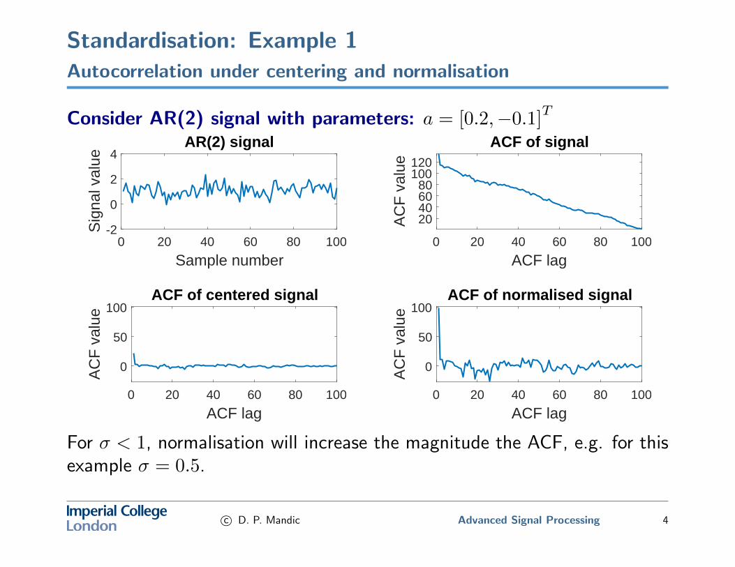
Consider AR(2) signal with parameters: a = [0.2,−0.1]T

0 20 40 60 80 100

Sample number

-2

0

2

4

Sig

nal v

alue

AR(2) signal

0 20 40 60 80 100

ACF lag

20406080

100120

AC

F v

alue

ACF of signal

0 20 40 60 80 100

ACF lag

0

50

100

AC

F v

alue

ACF of centered signal

0 20 40 60 80 100

ACF lag

0

50

100

AC

F v

alue

ACF of normalised signal

For σ < 1, normalisation will increase the magnitude the ACF, e.g. for thisexample σ = 0.5.


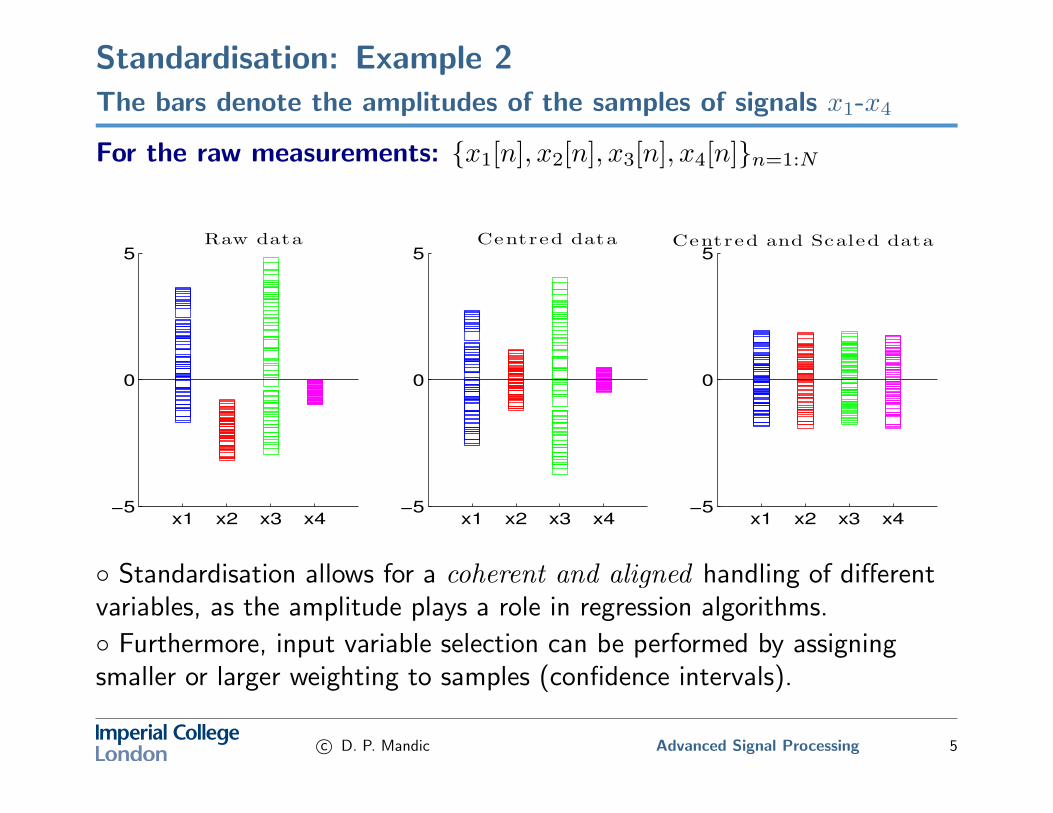
Standardisation: Example 2The bars denote the amplitudes of the samples of signals x1-x4

For the raw measurements: {x1[n], x2[n], x3[n], x4[n]}n=1:N

x1 x2 x3 x4−5

0

5

Raw data

x1 x2 x3 x4−5

0

5

Centred data

x1 x2 x3 x4−5

0

5Centred and Scaled data

◦ Standardisation allows for a coherent and aligned handling of differentvariables, as the amplitude plays a role in regression algorithms.

◦ Furthermore, input variable selection can be performed by assigningsmaller or larger weighting to samples (confidence intervals).


How do we describe a signal, statistically?

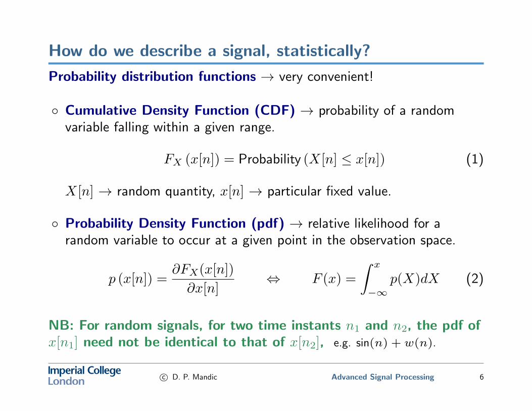
Probability distribution functions → very convenient!

◦ Cumulative Density Function (CDF) → probability of a randomvariable falling within a given range.

FX (x[n]) = Probability (X[n] ≤ x[n]) (1)

X[n] → random quantity, x[n] → particular fixed value.

◦ Probability Density Function (pdf) → relative likelihood for arandom variable to occur at a given point in the observation space.

p (x[n]) =∂FX(x[n])

∂x[n]⇔ F (x) =

∫ x

−∞p(X)dX (2)

NB: For random signals, for two time instants n1 and n2, the pdf ofx[n1] need not be identical to that of x[n2], e.g. sin(n) + w(n).


Statistical distributions: Uniform distribution

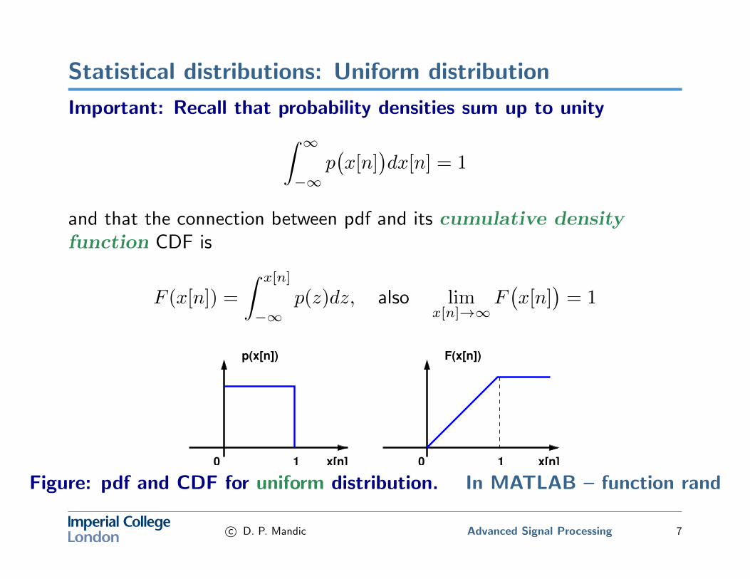
Important: Recall that probability densities sum up to unity∫ ∞−∞

p(x[n]

)dx[n] = 1

and that the connection between pdf and its cumulative densityfunction CDF is

F (x[n]) =

∫ x[n]

−∞p(z)dz, also lim

x[n]→∞F(x[n]

)= 1

0

p(x[n])

x[n]10

F(x[n])

x[n]1

Figure: pdf and CDF for uniform distribution. In MATLAB – function rand


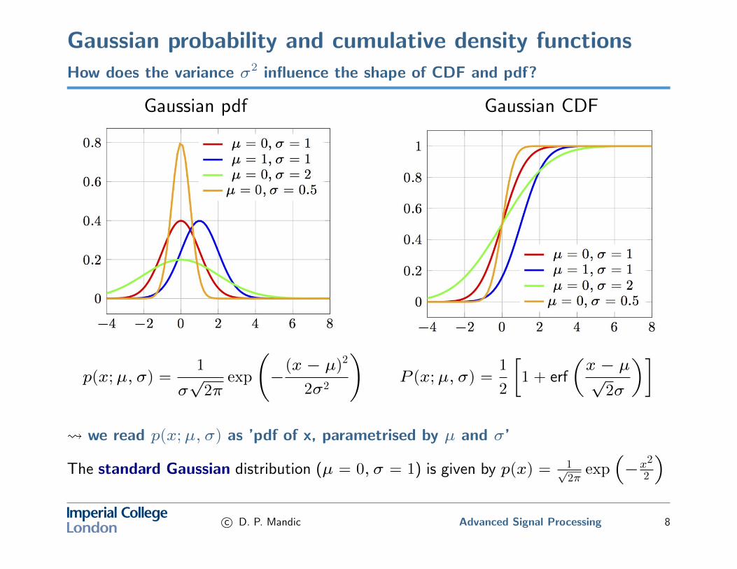
Gaussian probability and cumulative density functionsHow does the variance σ2 influence the shape of CDF and pdf?

Gaussian pdf Gaussian CDF

p(x;µ, σ) =1

σ√

2πexp

(−

(x− µ)2

2σ2

)P (x;µ, σ) =

1

2

[1 + erf

(x− µ√

2σ

)]

we read p(x;µ, σ) as ’pdf of x, parametrised by µ and σ’

The standard Gaussian distribution (µ = 0, σ = 1) is given by p(x) = 1√2π

exp(−x2

2

)c© D. P. Mandic Advanced Signal Processing 8

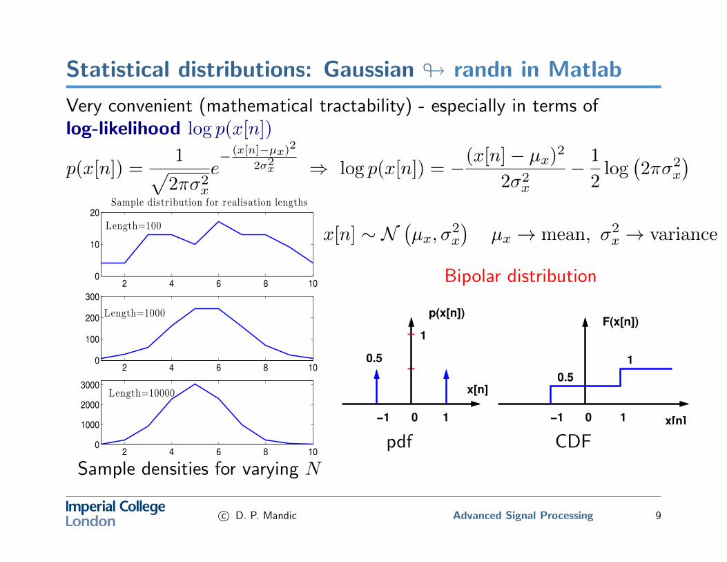
Statistical distributions: Gaussian # randn in Matlab

Very convenient (mathematical tractability) - especially in terms oflog-likelihood log p(x[n])

p(x[n]) =1√

2πσ2x

e−(x[n]−µx)2

2σ2x ⇒ log p(x[n]) = −(x[n]− µx)2

2σ2x

− 1

2log(2πσ2

x

)or x[n] ∼ N

(µx, σ

2x

)µx → mean, σ2

x → variance

2 4 6 8 100

10

20

Sample distr ibution for realisation lengths

Length=100

2 4 6 8 100

100

200

300

Length=1000

2 4 6 8 100

1000

2000

3000Length=10000

Sample densities for varying N

Bipolar distribution

10.5

1

p(x[n])F(x[n])

x[n]

−1 0 1 −1 0 1 x[n]

0.5

pdf CDF


Multi-dimensionality versus multi-variability

Univariate vs. Multivariate vs. Multidimensional

◦ Single input single output (SISO) e.g. single-sensor system

◦ Multiple input multiple output (MIMO) (arrays of transmitters andreceivers) can measure one source with many sensors

◦ Multidimensional processes (3D inertial bodymotion sensors, radar,vector fields, wind anemometers) – intrinsically multidimensional

Example: Multivariate function with single output (MISO)

stockvalue = f(stocks, oilprice,GNP,month, . . .)

⇒ Complete probabilistic description of {x[n]} is given by its pdf

p (x[n1], . . . , x[nk]) for all k and n1, . . . , nk.

Much research is being directed towards the reconstruction of the processhistory from observations of one variable only (Takens)


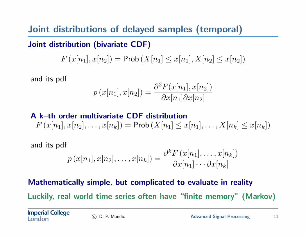
Joint distributions of delayed samples (temporal)

Joint distribution (bivariate CDF)

F (x[n1], x[n2]) = Prob (X[n1] ≤ x[n1], X[n2] ≤ x[n2])

and its pdf

p (x[n1], x[n2]) =∂2F (x[n1], x[n2])

∂x[n1]∂x[n2]

A k–th order multivariate CDF distributionF (x[n1], x[n2], . . . , x[nk]) = Prob (X[n1] ≤ x[n1], . . . , X[nk] ≤ x[nk])

and its pdf

p (x[n1], x[n2], . . . , x[nk]) =∂kF (x[n1], . . . , x[nk])

∂x[n1] · · · ∂x[nk]

Mathematically simple, but complicated to evaluate in reality

Luckily, real world time series often have “finite memory” (Markov)


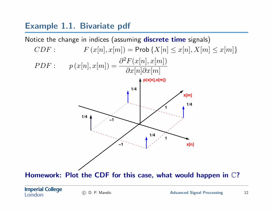
Example 1.1. Bivariate pdf

Notice the change in indices (assuming discrete time signals)

CDF : F (x[n], x[m]) = Prob {X[n] ≤ x[n], X[m] ≤ x[m]}

PDF : p (x[n], x[m]) =∂2F (x[n], x[m])

∂x[n]∂x[m]

1/4

x[m]

p(x[n],x[m])

x[n]

1

−1

1

−1

1/4

1/4

1/4

Homework: Plot the CDF for this case, what would happen in C?


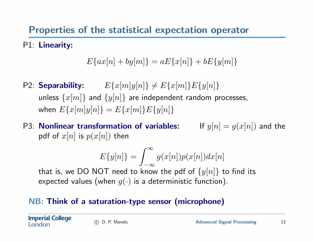
Properties of the statistical expectation operator

P1: Linearity:

E{ax[n] + by[m]} = aE{x[n]}+ bE{y[m]}

P2: Separability: E{x[m]y[n]} 6= E{x[m]}E{y[n]}unless {x[m]} and {y[n]} are independent random processes,

when E{x[m]y[n]} = E{x[m]}E{y[n]}

P3: Nonlinear transformation of variables: If y[n] = g(x[n]) and thepdf of x[n] is p(x[n]) then

E{y[n]} =

∫ ∞−∞

g(x[n])p(x[n])dx[n]

that is, we DO NOT need to know the pdf of {y[n]} to find itsexpected values (when g(·) is a deterministic function).

NB: Think of a saturation-type sensor (microphone)


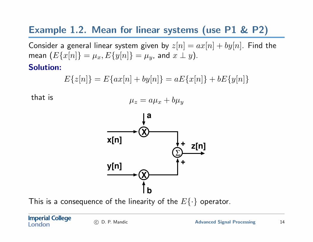
Example 1.2. Mean for linear systems (use P1 & P2)

Consider a general linear system given by z[n] = ax[n] + by[n]. Find themean (E{x[n]} = µx, E{y[n]} = µy, and x ⊥ y).

Solution:

E{z[n]} = E{ax[n] + by[n]} = aE{x[n]}+ bE{y[n]}

that is µz = aµx + bµy

X

x[n]

y[n]

z[n]

a

b

+

+

X

Σ

This is a consequence of the linearity of the E{·} operator.


Example 1.3. Mean for nonlinear systems (use P3)think about e.g. estimating the variance empirically

For a nonlinear system, say the sensor nonlinearity is given by

z[n] = x2[n]

using Property P3 of the statistical expectation operator, we have

µz = E{x2[n]} =

∫ ∞−∞

x2[n]p(x[n])dx[n]

This is extremely useful, since most of the real–world signals are observedthrough sensors, e.g.

microphones, geophones, various probes ...

which are almost invariably nonlinear (typically a saturation typenonlinearity)


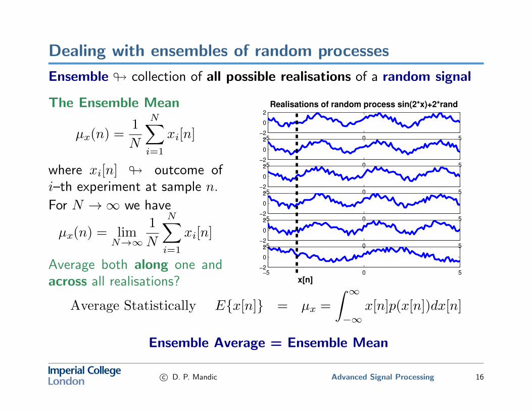
Dealing with ensembles of random processes

Ensemble # collection of all possible realisations of a random signal

The Ensemble Mean

µx(n) =1

N

N∑i=1

xi[n]

where xi[n] # outcome ofi–th experiment at sample n.

For N →∞ we have

µx(n) = limN→∞

1

N

N∑i=1

xi[n]

Average both along one andacross all realisations?

−5 0 5−2

0

2

−5 0 5−2

0

2

Realisations of random process sin(2*x)+2*rand

−5 0 5−2

0

2

−5 0 5−2

0

2

−5 0 5−2

0

2

−5 0 5−2

0

2

x[n]

Average Statistically E{x[n]} = µx =

∫ ∞−∞

x[n]p(x[n])dx[n]

Ensemble Average = Ensemble Mean


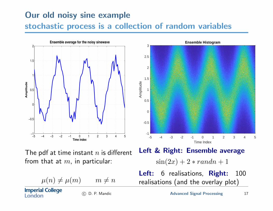
Our old noisy sine examplestochastic process is a collection of random variables

−5 −4 −3 −2 −1 0 1 2 3 4 5−1

−0.5

0

0.5

1

1.5

2

Time index

Am

pli

tud

e

Ensemble average for the noisy sinewave

The pdf at time instant n is differentfrom that at m, in particular:

µ(n) 6= µ(m) m 6= n

Ensemble Histogram

-5 -4 -3 -2 -1 0 1 2 3 4 5

Time Index

-1

-0.5

0

0.5

1

1.5

2

2.5

3

Am

plit

ude

Left & Right: Ensemble average

sin(2x) + 2 ∗ randn+ 1

Left: 6 realisations, Right: 100realisations (and the overlay plot)


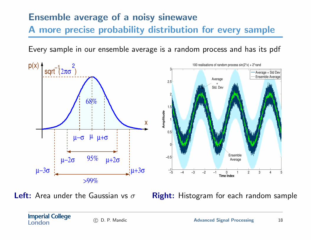
Ensemble average of a noisy sinewaveA more precise probability distribution for every sample

Every sample in our ensemble average is a random process and has its pdf

2p(x)

x

µ µ+σµ−σ

µ+2σµ−2σ

µ+3σµ−3σ

2πσ

68%

95%

>99%

sqrt ( )−1

−5 −4 −3 −2 −1 0 1 2 3 4 5−1

−0.5

0

0.5

1

1.5

2

2.5

3

Time Index

Am

pli

tud

e

100 realisations of random process sin(2*x) + 2*rand

Average + Std DevEnsemble Average

Ensemble Average

Average+

Std. Dev

Left: Area under the Gaussian vs σ Right: Histogram for each random sample


Second order statistics: 1) Correlation

• Correlation (also known as Autocorrelation Function (ACF))r(m,n) = E{x[m]x[n]}, that is

r(m,n) =

∫ ∞−∞

x[m]x[n]p(x[m], x[n]

)dx[m]dx[n]

◦ in practice, for ergodic signals we calculate correlations from therelative frequency perspective

r(m,n) = limN→∞

{1

N

N∑i=1

xi[m]xi[n]

}, (i denotes the ensemble index)

◦ r(m,n) measures the degree of similarity between x[n] and x[m].◦ r(n, n) = E{x2[n]} ⇒ is the average ”power” of a signal◦ r(m,n) = r(n,m) ⇒ the autocorrelation matrix of all {r(m,n)}

R = {r(m,n)} = E[xxH

]is symmetric


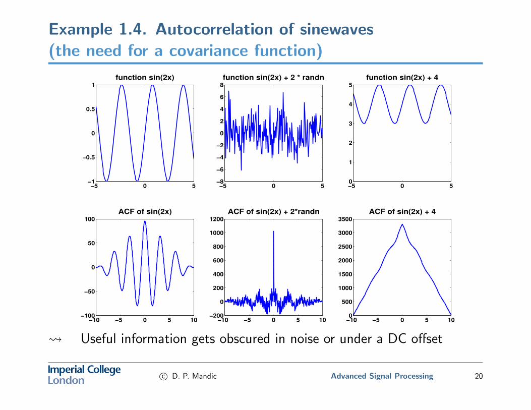
Example 1.4. Autocorrelation of sinewaves(the need for a covariance function)

−5 0 5−1

−0.5

0

0.5

1

function sin(2x)

−5 0 5−8

−6

−4

−2

0

2

4

6

8

function sin(2x) + 2 * randn

−5 0 50

1

2

3

4

5

function sin(2x) + 4

−10 −5 0 5 10−100

−50

0

50

100

ACF of sin(2x)

−10 −5 0 5 10−200

0

200

400

600

800

1000

1200

ACF of sin(2x) + 2*randn

−10 −5 0 5 100

500

1000

1500

2000

2500

3000

3500

ACF of sin(2x) + 4

Useful information gets obscured in noise or under a DC offset


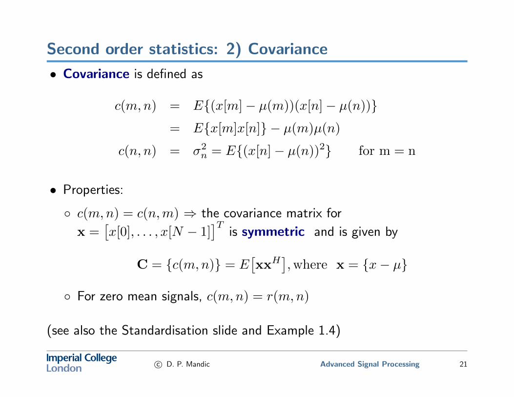
Second order statistics: 2) Covariance

• Covariance is defined as

c(m,n) = E{(x[m]− µ(m))(x[n]− µ(n))}= E{x[m]x[n]} − µ(m)µ(n)

c(n, n) = σ2n = E{(x[n]− µ(n))2} for m = n

• Properties:

◦ c(m,n) = c(n,m) ⇒ the covariance matrix for

x =[x[0], . . . , x[N − 1]

]Tis symmetric and is given by

C = {c(m,n)} = E[xxH

],where x = {x− µ}

◦ For zero mean signals, c(m,n) = r(m,n)

(see also the Standardisation slide and Example 1.4)


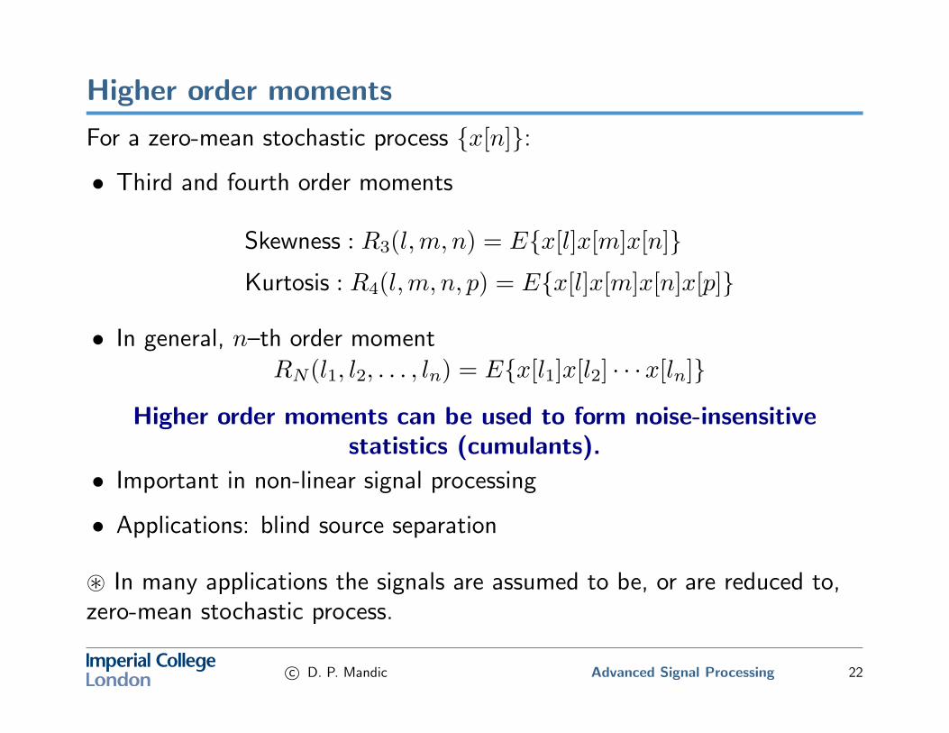
Higher order moments

For a zero-mean stochastic process {x[n]}:

• Third and fourth order moments

Skewness : R3(l,m, n) = E{x[l]x[m]x[n]}Kurtosis : R4(l,m, n, p) = E{x[l]x[m]x[n]x[p]}

• In general, n–th order moment

RN(l1, l2, . . . , ln) = E{x[l1]x[l2] · · ·x[ln]}

Higher order moments can be used to form noise-insensitivestatistics (cumulants).

• Important in non-linear signal processing

• Applications: blind source separation

~ In many applications the signals are assumed to be, or are reduced to,zero-mean stochastic process.


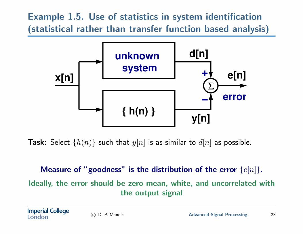
Example 1.5. Use of statistics in system identification(statistical rather than transfer function based analysis)

Σ

−

+systemunknown

error

e[n]

y[n]

d[n]

{ h(n) }

x[n]

Task: Select {h(n)} such that y[n] is as similar to d[n] as possible.

Measure of ”goodness” is the distribution of the error {e[n]}.

Ideally, the error should be zero mean, white, and uncorrelated withthe output signal


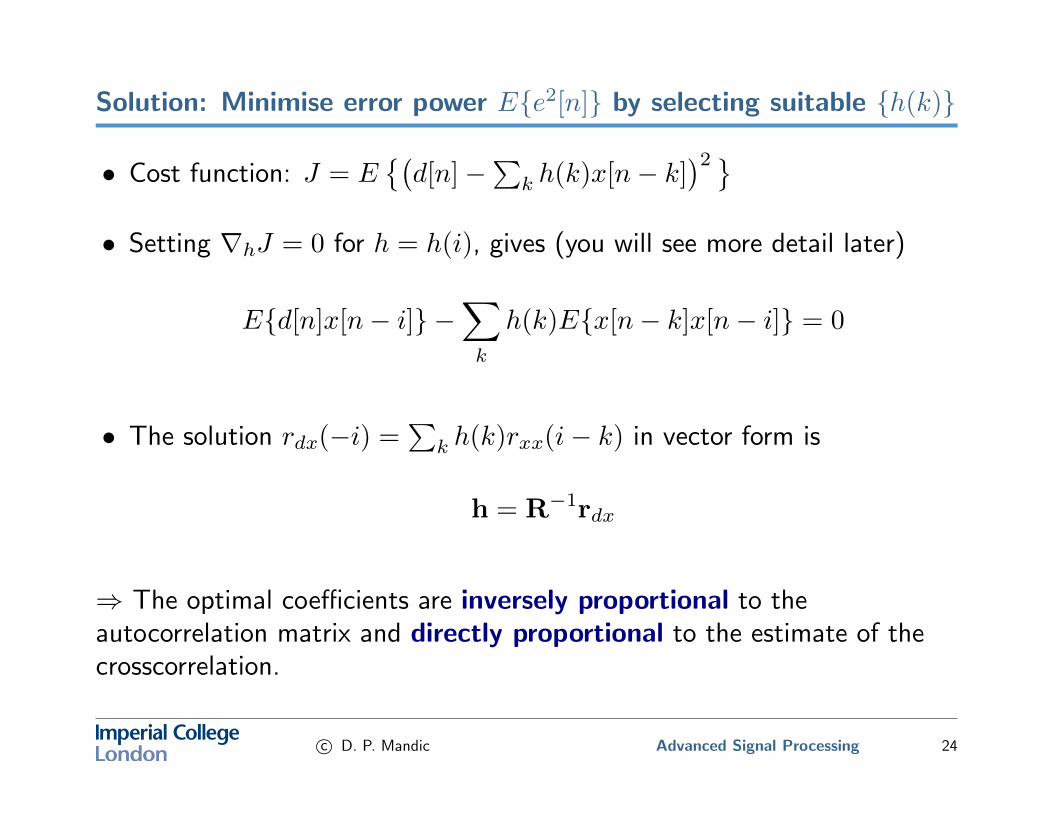
Solution: Minimise error power E{e2[n]} by selecting suitable {h(k)}

• Cost function: J = E{(d[n]−

∑k h(k)x[n− k]

)2 }• Setting ∇hJ = 0 for h = h(i), gives (you will see more detail later)

E{d[n]x[n− i]} −∑k

h(k)E{x[n− k]x[n− i]} = 0

• The solution rdx(−i) =∑k h(k)rxx(i− k) in vector form is

h = R−1rdx

⇒ The optimal coefficients are inversely proportional to theautocorrelation matrix and directly proportional to the estimate of thecrosscorrelation.


Independence, uncorrelatedness and orthogonality

• Two RV are independent if the realisation of one does not affect thedistribution of the other, consequently, the joint density is separable:

p(x, y) = p(x)p(y)

Example: Sunspot numbers on 31 December and Argentinian debt

• Two RVs are uncorrelated if their cross-covariance is zero, that is

c(x, y) = E[(x− µx)(y − µy)] = E[xy]− E[x]E[y] = 0

Example: x ∼ N (0, 1) and y = x2 (impossible to relate through alinear relationship)

• Two RV are orthogonal if r(x, y) = E[xy] = 0

Example: Two uncorrelated RVs with at least one of them zero-mean


Independence, uncorrelatedness and orthogonality -Properties

• Independent RVs are always uncorrelated

• Uncorrelatedness can be seen as a ’weaker’ form of independence sinceonly the expectation (rather than the density) needs to be separable.

• Uncorrelatedness is a measure of linear independence. For instance,x ∼ N (0, 1) and y = x2 are clearly dependent but uncorrelated,meaning that there is no linear relationship between them

• Since cxy = rxy −mxmy orthogonal RVs x and y need not beuncorrelated. Furthermore:

– uncorrelated if they are independent and one them is zero mean– orthogonal if they are uncorrelated and one them is zero mean

• For uncorrelated random variables: var{x+ y} = var{x}+ var{y}


Stationarity: Strict and wide sense

• Strict Sense Stationarity (SSS): The process {x[n]} is SSS if for allk the joint distribution p(x[n1], . . . , x[nk]) is invariant under timeshifts, i.e. (all moments considered)

p (x[n1 + n0], . . . , x[nk + n0]) = p (x[n1], . . . , x[nk]) ,∀n0

As SSS is too strict for practical applications, we consider themore ’relaxed’ stationarity condition.

• Wide-Sense Stationarity (WSS): The process {x[n]} is WSS if ∀m,n:

◦ Mean: E{x[m]} = E{x[m+ n]},◦ Covariance: c(m,n) = c(m− n, 0) = c(m− n)

Note that only the first two moments are considered.

Example of WSS: x[n] = sin(2πfn+ φ), where φ is uniformly distributedon [−π, π]


Autocorrelation function r(m) of WSS processes

i) Time/shift invariant: r(m,n) = r(m− n, 0) = r(m− n) (followsfrom the covariance WSS requirement)

ii) Symmetric: r(−m) = r(m) (follows from the definition)

iii) r(0) ≥ |r(m)| (maximum at m = 0)

The signal power = r(0) # Parseval’s relationship

Follows from E{(x[n]− λx[n+m])2} ≥ 0, i.e.

E{x2[n]} − 2λE{x[n]x[n+m]}+ λ2E{x2[n+m]} ≥ 0 ∀λ

r(0)− 2λr(m) + λ2r(0) ≥ 0 ∀λ

which is quadratic in λ and required to be positive for all λ, i.e. theequation determinant: ∆ = r2(m)− r(0)r(0) ≤ 0⇒ r(0) ≥ |r(m)|.


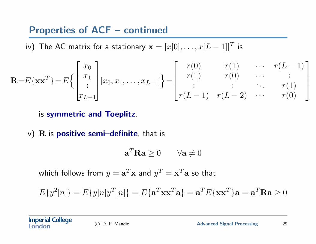
Properties of ACF – continued

iv) The AC matrix for a stationary x = [x[0], . . . , x[L− 1]]T is

R=E{xxT}=E{

x0x1...

xL−1

[x0, x1, . . . , xL−1]}

=

r(0) r(1) · · · r(L− 1)r(1) r(0) · · · ...

... ... . . . r(1)r(L− 1) r(L− 2) · · · r(0)

is symmetric and Toeplitz.

v) R is positive semi–definite, that is

aTRa ≥ 0 ∀a 6= 0

which follows from y = aTx and yT = xTa so that

E{y2[n]} = E{y[n]yT [n]} = E{aTxxTa} = aTE{xxT}a = aTRa ≥ 0


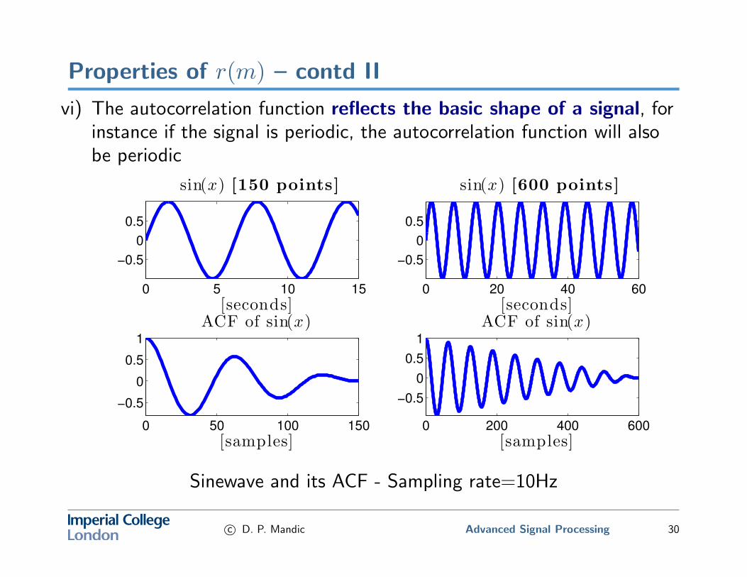
Properties of r(m) – contd II

vi) The autocorrelation function reflects the basic shape of a signal, forinstance if the signal is periodic, the autocorrelation function will alsobe periodic

0 5 10 15

−0.5

0

0.5

[seconds]

sin(x) [150 points]

0 20 40 60

−0.5

0

0.5

[seconds]

sin(x) [600 points]

0 50 100 150

−0.5

0

0.5

1

[samples]

ACF of sin(x)

0 200 400 600

−0.5

0

0.5

1

[samples]

ACF of sin(x)

Sinewave and its ACF - Sampling rate=10Hz


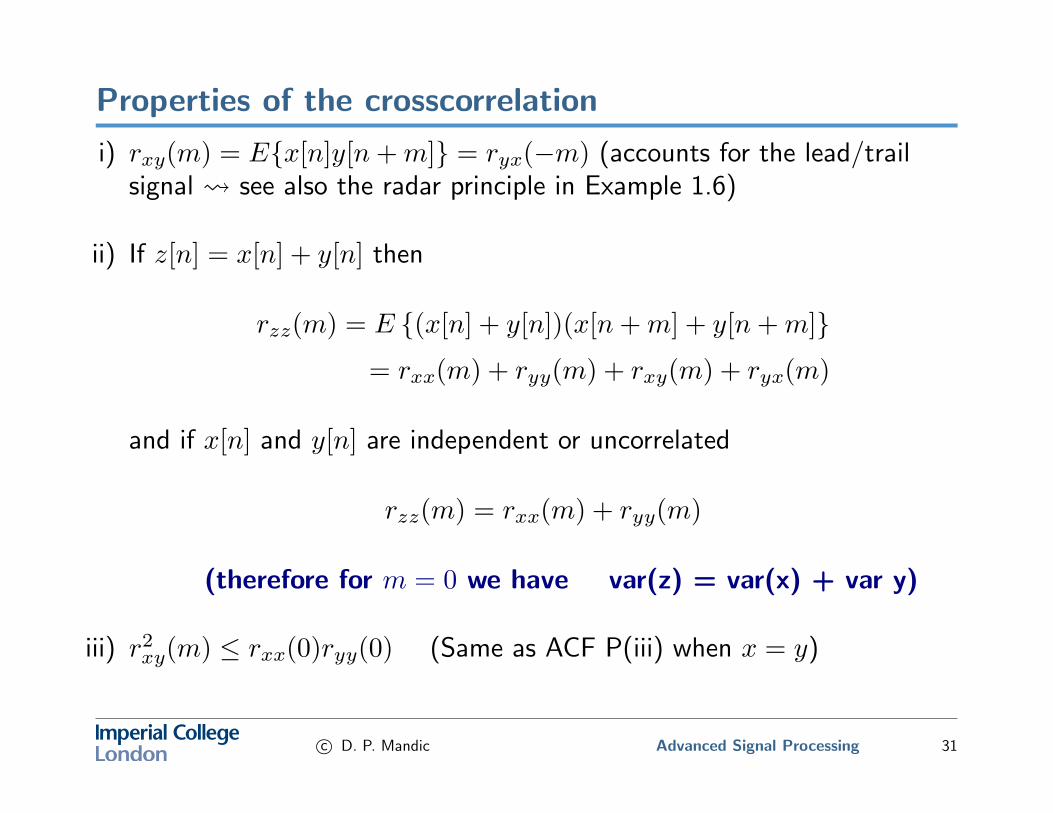
Properties of the crosscorrelation

i) rxy(m) = E{x[n]y[n+m]} = ryx(−m) (accounts for the lead/trailsignal see also the radar principle in Example 1.6)

ii) If z[n] = x[n] + y[n] then

rzz(m) = E {(x[n] + y[n])(x[n+m] + y[n+m]}= rxx(m) + ryy(m) + rxy(m) + ryx(m)

and if x[n] and y[n] are independent or uncorrelated

rzz(m) = rxx(m) + ryy(m)

(therefore for m = 0 we have var(z) = var(x) + var y)

iii) r2xy(m) ≤ rxx(0)ryy(0) (Same as ACF P(iii) when x = y)


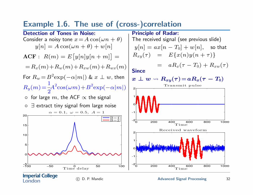
Example 1.6. The use of (cross-)correlationDetection of Tones in Noise:Consider a noisy tone x=A cos(ωn+ θ)

y[n] = A cos(ωn+ θ) + w[n]

ACF : R(m) = E[y[n]y[n+m]

]=

=Rx(m)+Rw(m)+Rxw(m)+Rwx(m)

For Rw=B2exp(−α|m|) & x ⊥ w, then

Ry(m)=1

2A

2cos(ωm)+B

2exp(−α|m|)

◦ for large m, the ACF ∝ the signal

◦ ∃ extract tiny signal from large noise

−100 −50 0 50 100−5

0

5

10

15

20

α = 0.1, ω = 0.5, A = 1

Time delay

B=4B=2

Principle of Radar:The received signal (see previous slide)

y[n] = ax[n− T0] + w[n], so that

Rxy(τ) = E{x(n)y(n+ τ)}

= aRx(τ − T0) + Rxw(τ)Since

x ⊥ w Rxy(τ )=aRx(τ − T0)

0 200 400 600 800 1000−2

−1

0

1

2

Time

Transmit pulse

0 200 400 600 800 1000−2

−1

0

1

2

Time

Received waveform


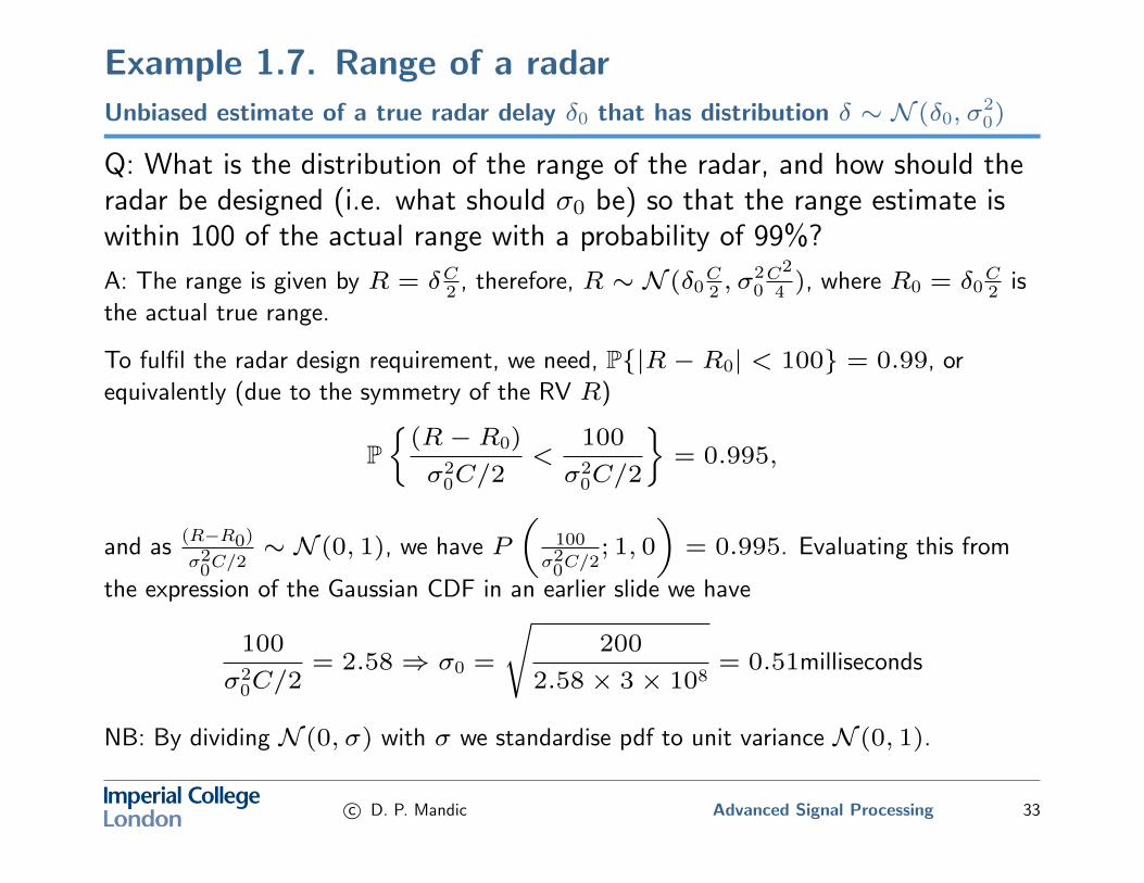
Example 1.7. Range of a radarUnbiased estimate of a true radar delay δ0 that has distribution δ ∼ N (δ0, σ

20)

Q: What is the distribution of the range of the radar, and how should theradar be designed (i.e. what should σ0 be) so that the range estimate iswithin 100 of the actual range with a probability of 99%?

A: The range is given by R = δC2 , therefore, R ∼ N (δ0C2 , σ

20C2

4 ), where R0 = δ0C2 is

the actual true range.

To fulfil the radar design requirement, we need, P{|R− R0| < 100} = 0.99, or

equivalently (due to the symmetry of the RV R)

P{(R− R0)

σ20C/2

<100

σ20C/2

}= 0.995,

and as(R−R0)

σ20C/2∼ N (0, 1), we have P

(100

σ20C/2; 1, 0

)= 0.995. Evaluating this from

the expression of the Gaussian CDF in an earlier slide we have

100

σ20C/2

= 2.58⇒ σ0 =

√200

2.58× 3× 108= 0.51milliseconds

NB: By dividing N (0, σ) with σ we standardise pdf to unit variance N (0, 1).


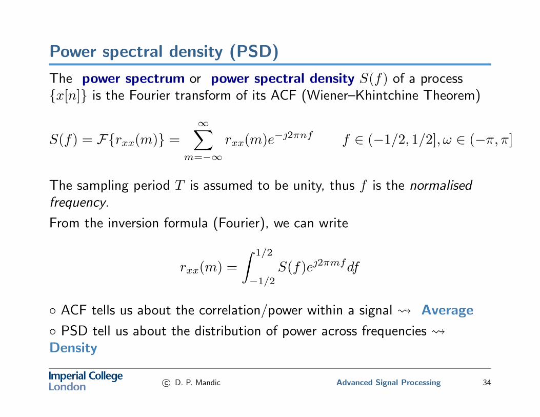
Power spectral density (PSD)

The power spectrum or power spectral density S(f) of a process{x[n]} is the Fourier transform of its ACF (Wiener–Khintchine Theorem)

S(f) = F{rxx(m)} =

∞∑m=−∞

rxx(m)e−2πnf f ∈ (−1/2, 1/2], ω ∈ (−π, π]

The sampling period T is assumed to be unity, thus f is the normalisedfrequency.

From the inversion formula (Fourier), we can write

rxx(m) =

∫ 1/2

−1/2S(f)e2πmfdf

◦ ACF tells us about the correlation/power within a signal Average

◦ PSD tell us about the distribution of power across frequencies Density


PSD properties

i) S(f) is a positive real function (it is a distribution) ⇒ S(f) = S∗(f).Since r(−m) = r(m) we can write

S(f) =

∞∑m=−∞

rxx(−m)e2πmf =

∞∑m=−∞

rxx(m)e−2πmf

and hence

S(f) =

∞∑m=−∞

rxx(m) cos(2πmf) = rxx(0) + 2

∞∑m=1

rxx(m) cos(2πmf)

ii) S(f) is a symmetric function, S(−f) = S(f). This follows from thelast expression.

iii) r(0) =∫ 1/2

−1/2 S(f)df = E{x2[n]} ≥ 0.

⇒ the area below the PSD (power spectral density) curve = Signal Power.


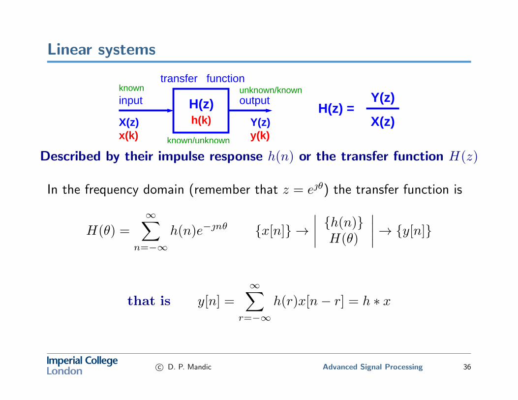
Linear systems

H(z)X(z)

Y(z)H(z) =

unknown/known

known/unknown

knownfunctiontransfer

outputinput

h(k)y(k)x(k)Y(z)X(z)

Described by their impulse response h(n) or the transfer function H(z)

In the frequency domain (remember that z = eθ) the transfer function is

H(θ) =

∞∑n=−∞

h(n)e−nθ {x[n]} →∣∣∣∣ {h(n)}H(θ)

∣∣∣∣→ {y[n]}

that is y[n] =

∞∑r=−∞

h(r)x[n− r] = h ∗ x


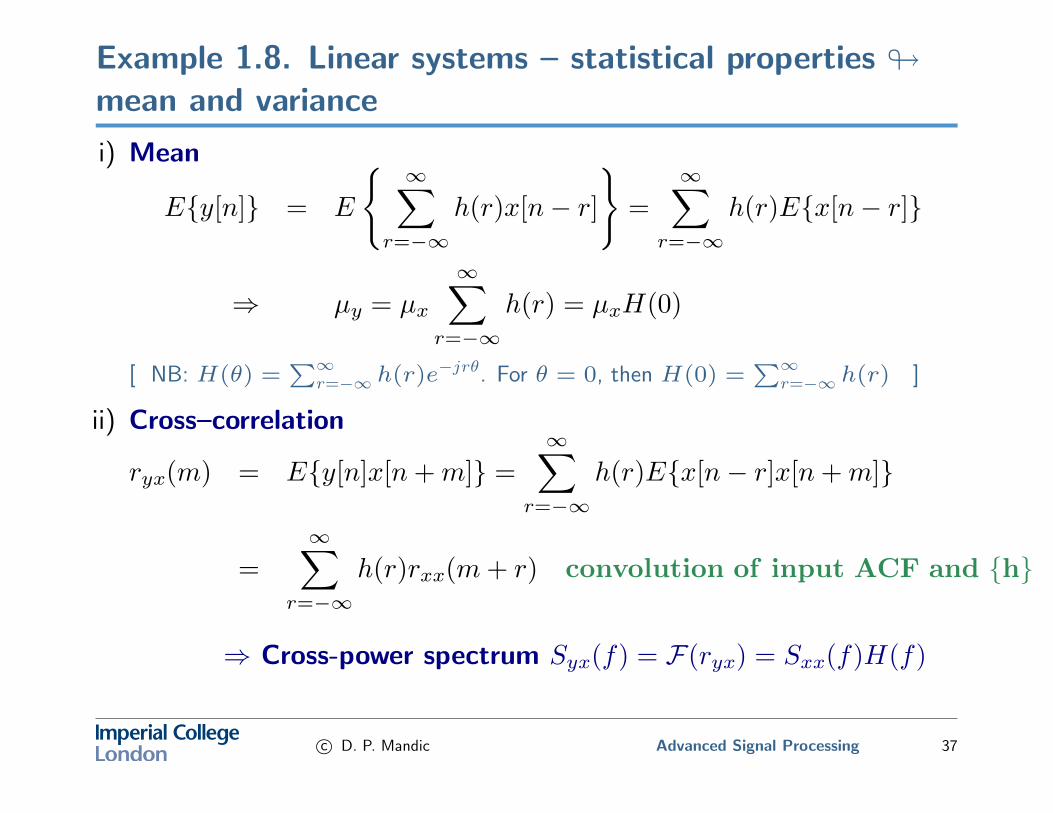
Example 1.8. Linear systems – statistical properties #mean and variance

i) Mean

E{y[n]} = E

{ ∞∑r=−∞

h(r)x[n− r]

}=

∞∑r=−∞

h(r)E{x[n− r]}

⇒ µy = µx

∞∑r=−∞

h(r) = µxH(0)

[ NB: H(θ) =∑∞

r=−∞ h(r)e−jrθ. For θ = 0, then H(0) =

∑∞r=−∞ h(r) ]

ii) Cross–correlation

ryx(m) = E{y[n]x[n+m]} =

∞∑r=−∞

h(r)E{x[n− r]x[n+m]}

=

∞∑r=−∞

h(r)rxx(m+ r) convolution of input ACF and {h}

⇒ Cross-power spectrum Syx(f) = F(ryx) = Sxx(f)H(f)


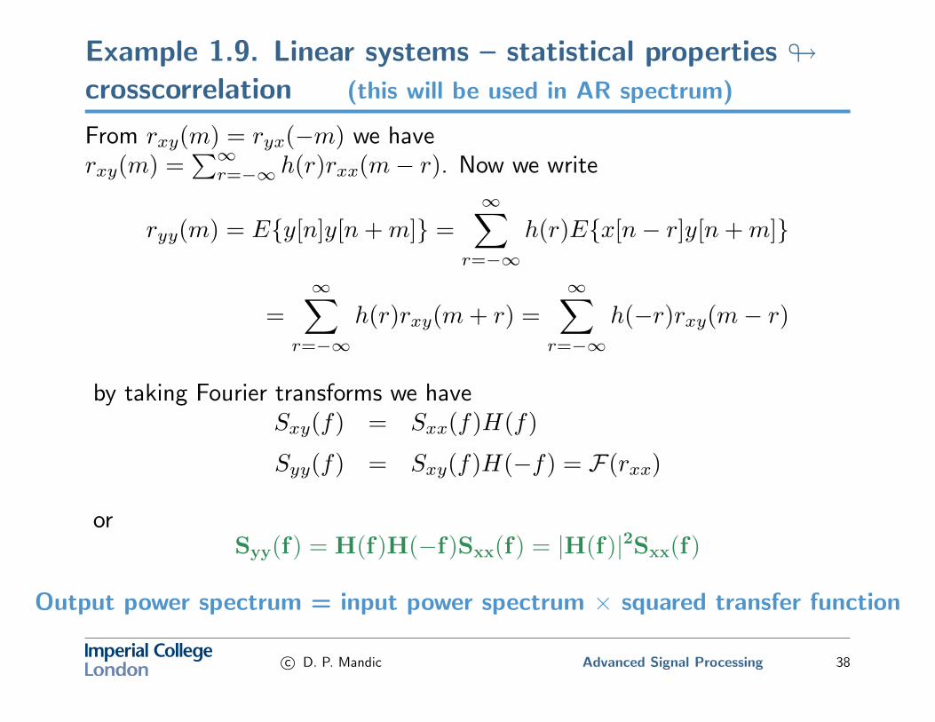
Example 1.9. Linear systems – statistical properties #crosscorrelation (this will be used in AR spectrum)

From rxy(m) = ryx(−m) we haverxy(m) =

∑∞r=−∞ h(r)rxx(m− r). Now we write

ryy(m) = E{y[n]y[n+m]} =

∞∑r=−∞

h(r)E{x[n− r]y[n+m]}

=

∞∑r=−∞

h(r)rxy(m+ r) =

∞∑r=−∞

h(−r)rxy(m− r)

by taking Fourier transforms we haveSxy(f) = Sxx(f)H(f)

Syy(f) = Sxy(f)H(−f) = F(rxx)

orSyy(f) = H(f)H(−f)Sxx(f) = |H(f)|2Sxx(f)

Output power spectrum = input power spectrum × squared transfer function


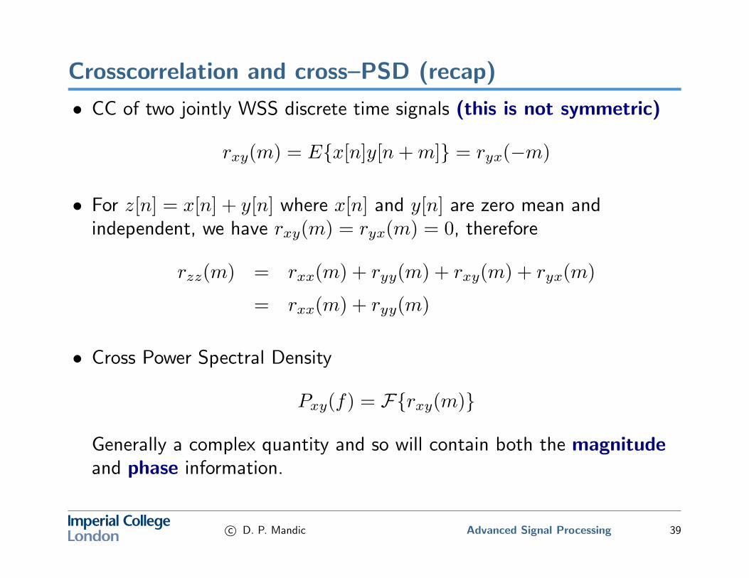
Crosscorrelation and cross–PSD (recap)

• CC of two jointly WSS discrete time signals (this is not symmetric)

rxy(m) = E{x[n]y[n+m]} = ryx(−m)

• For z[n] = x[n] + y[n] where x[n] and y[n] are zero mean andindependent, we have rxy(m) = ryx(m) = 0, therefore

rzz(m) = rxx(m) + ryy(m) + rxy(m) + ryx(m)

= rxx(m) + ryy(m)

• Cross Power Spectral Density

Pxy(f) = F{rxy(m)}

Generally a complex quantity and so will contain both the magnitudeand phase information.


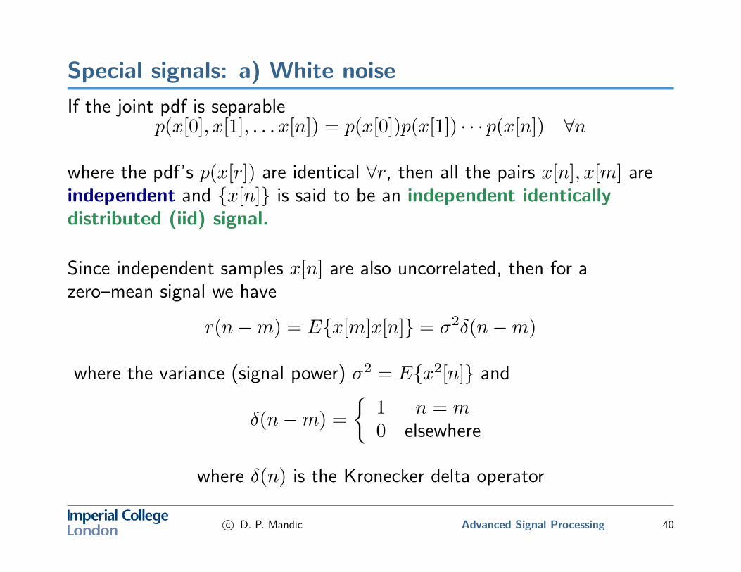
Special signals: a) White noise

If the joint pdf is separablep(x[0], x[1], . . . x[n]) = p(x[0])p(x[1]) · · · p(x[n]) ∀n

where the pdf’s p(x[r]) are identical ∀r, then all the pairs x[n], x[m] areindependent and {x[n]} is said to be an independent identicallydistributed (iid) signal.

Since independent samples x[n] are also uncorrelated, then for azero–mean signal we have

r(n−m) = E{x[m]x[n]} = σ2δ(n−m)

where the variance (signal power) σ2 = E{x2[n]} and

δ(n−m) =

{1 n = m0 elsewhere

where δ(n) is the Kronecker delta operator


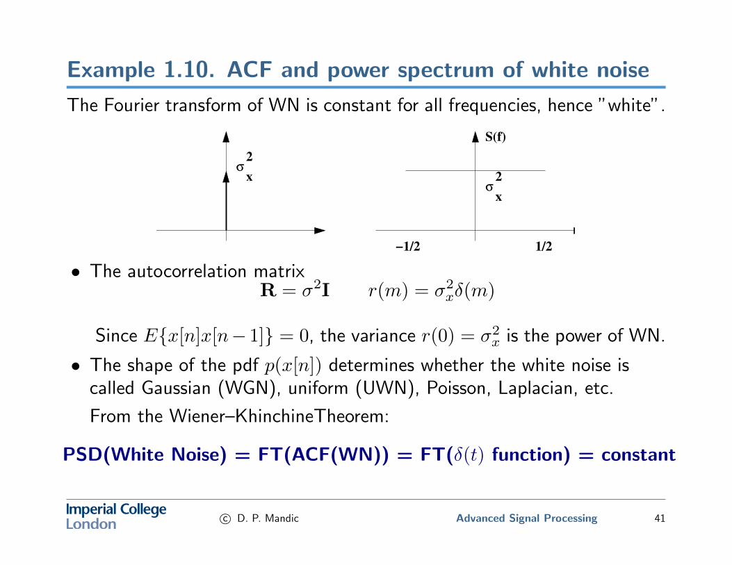
Example 1.10. ACF and power spectrum of white noise

The Fourier transform of WN is constant for all frequencies, hence ”white”.

σ

−1/2 1/2

2

xσ

S(f)

2

x

• The autocorrelation matrixR = σ2I r(m) = σ2

xδ(m)

Since E{x[n]x[n− 1]} = 0, the variance r(0) = σ2x is the power of WN.

• The shape of the pdf p(x[n]) determines whether the white noise iscalled Gaussian (WGN), uniform (UWN), Poisson, Laplacian, etc.

From the Wiener–KhinchineTheorem:

PSD(White Noise) = FT(ACF(WN)) = FT(δ(t) function) = constant


b) First order Markov signals: autoregressive modelling

(finite memory in the description of a random signal)

If instead of the iid condition, we have the first order conditionalexpectation, then

p(x[n], x[n− 1], x[n− 2], . . . , x[0]) = p(x[n]|x[n− 1])

where p(a|b) is defined as the pdf of ”a” conditioned upon the (possiblycorrelated) observation ”b”

⇒ the signal above is the first order Markov signal.

Example: Examine the statistical properties of the signal given by

y[n] = ay[n− 1] + w[n]

where a = 0.8 and w[n] ∼ N (0, 1) (see your coursework).


c) Minimum phase signals

Let {x[n]} be observed for n = 0, 1, . . . , N − 1.

X(z) = x[0] + x[1]z−1 + · · ·+ x[N − 1]z−(N−1) =

A

N∏i=1

(1− ziz−1

), A(0) = x[0]

• |zi| ≤ 1, ∀i then X(z) is said to be minimum phase

• |zi| ≥ 1, ∀i, then X(z) is said to be maximum phase

• |zi| ≥ 0 for some i while for others |zi| ≤ 1 then X(z) is said to be ofmixed phase.

In DSP, the algorithms often rely on the minimum phase property of asignal for stability (of the inverse system) and to be able to have real-timeimplementation (causality).


d) Gaussian random signals

A signal in which each of the L samples is Gaussian distributed

p(x[i]) =1√

2πσ2i

e(x[i]−µ(i))2

2σ2i i = 0, . . . , L− 1

denoted by N (µ(i), σ2i ).

The joint pdf of L samples x[n0], x[n1], . . . , x[nL−1] is then

p(x) = p(x[n0], x[n1], . . . , x[nL−1])

p(x) =1

[2π]L/2det(C)1/2e(x−µ)TC−1(x−µ)

2 =1

(2πσ2)L/2e

[− 1

2σ2

∑L−1n=0(x[n]−µ)

2]

where x = [x[n0], x[n1], . . . , x[nL−1]], µ = [µ[n0], µ[n1], . . . , µ[nL−1]] andC is a covariance matrix with determinant ∆.


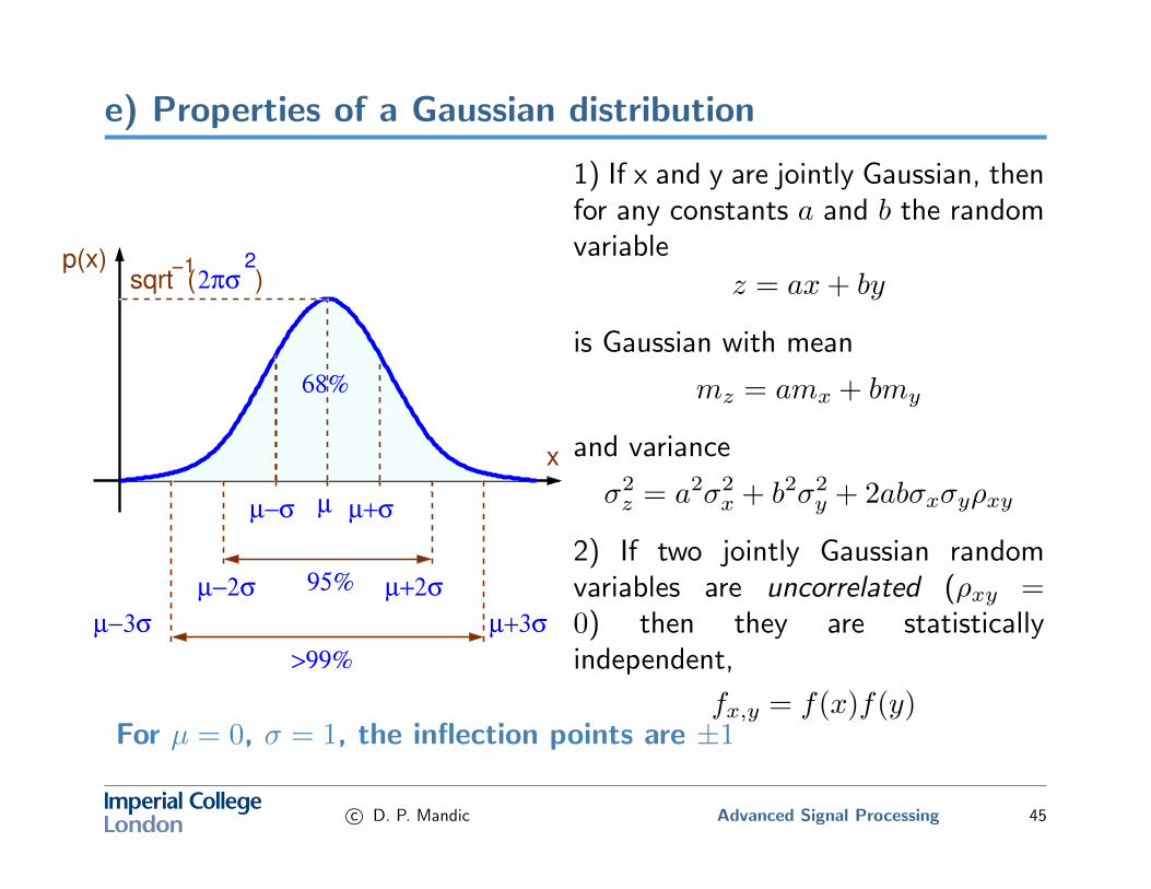
e) Properties of a Gaussian distribution

2p(x)

x

µ µ+σµ−σ

µ+2σµ−2σ

µ+3σµ−3σ

2πσ

68%

95%

>99%

sqrt ( )−1

1) If x and y are jointly Gaussian, thenfor any constants a and b the randomvariable

z = ax+ by

is Gaussian with mean

mz = amx + bmy

and variance

σ2z = a2σ2

x + b2σ2y + 2abσxσyρxy

2) If two jointly Gaussian randomvariables are uncorrelated (ρxy =0) then they are statisticallyindependent,

fx,y = f(x)f(y)For µ = 0, σ = 1, the inflection points are ±1


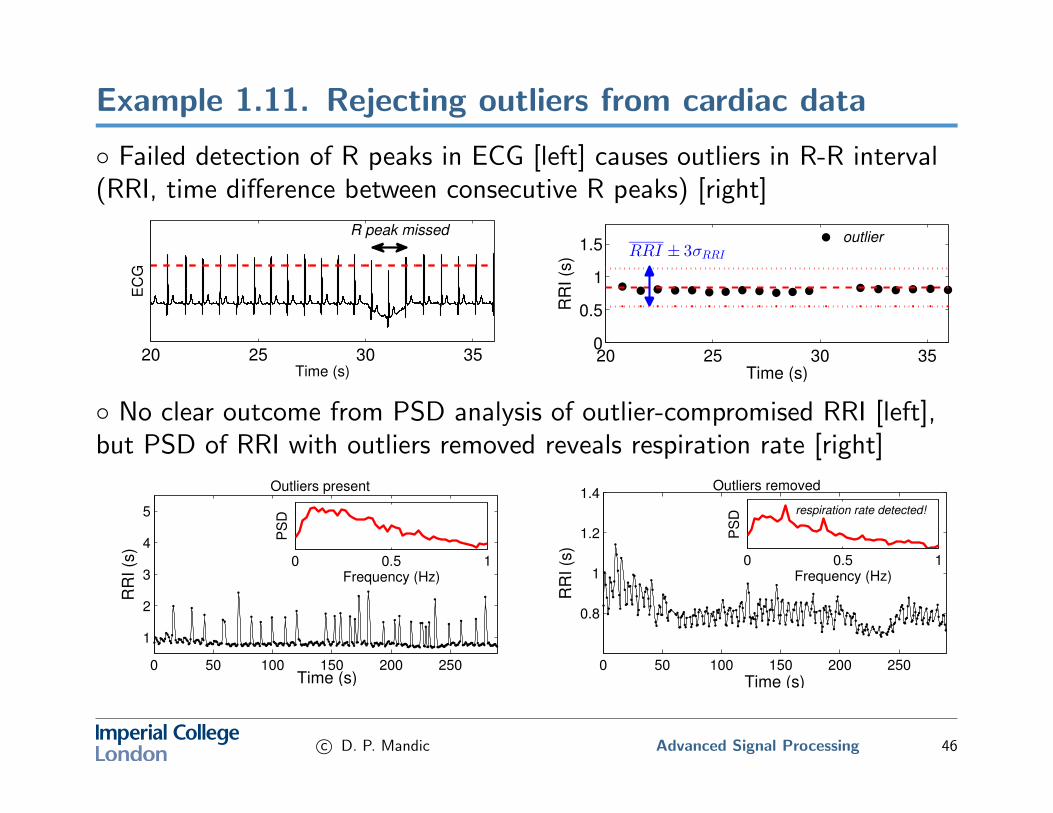
Example 1.11. Rejecting outliers from cardiac data

◦ Failed detection of R peaks in ECG [left] causes outliers in R-R interval(RRI, time difference between consecutive R peaks) [right]

20 25 30 35

EC

G

Time (s)

R peak missed

20 25 30 350

0.5

1

1.5

RR

I (s

)

Time (s)

RRI ± 3σRRI

outlier

◦ No clear outcome from PSD analysis of outlier-compromised RRI [left],but PSD of RRI with outliers removed reveals respiration rate [right]

0 50 100 150 200 250

1

2

3

4

5

Time (s)

RR

I (s

)

Outliers present

0 0.5 1Frequency (Hz)

PS

D

0 50 100 150 200 250

0.8

1

1.2

1.4Outliers removed

Time (s)

RR

I (s

)0 0.5 1

Frequency (Hz)

PS

D respiration rate detected!


f) Conditional mean estimator for Gaussian randomvariables

3) If x and y are jointly Gaussian random variables then the optimumestimator for y, given by

y = g(x)

that minimizes the mean square error ξ = E{[y = g(x)]2} is a linearestimator in the form

y = ax+ b

4) If x is Gaussian with zero mean then

E{xn} =

{1× 3× 5× · · · × (n− 1)σnx , n even0, n odd


e) Ergodic signals

In practice, we often have only one observation of a signal (real–time)

Then, statistical averages are replaced by time averages.

This is necessary because

◦ ensemble averages are generally unknown a priori

◦ only a single realisation of the random signal is often available

Thus, the ensemble average

mx(n) = 1L

∑Li=1 xi(n)

is therefore replaced by a time average

mx(N) = 1N

∑N−1n=0 x(n)


e) Ergodic signals – Example

Consider the random processx(n) = Acos(nω0)

where A is a random variable that is equally likely to assume the value of 1or 2.

The mean of this process is

E{x(n)} = E{A}cos(nω0) = 1.5cos(nω0)

However, for a single realisation of this process, for large N , the samplemean is approximately zero

mx ≈ 0, N >> 1

⇒ x(n) is not ergodic and therefore the statistical expectationcannot be computed using time averages on a single realisation.


e) Ergodicity in the mean

Definition: If the sample mean mx(N) of a WSS process converges tomx, in the mean–square sense, then the process is said to be ergodic inthe mean, and we write

limN→∞ mx(N) = mx

For the convergence of the sample mean in the mean–square sense

◦ Asymptotically unbiased

limN→∞E{mx(N)} = mx

Consider the variance of the estimate → 0 as N →∞limN→∞ V ar{mx(N)} = 0 (consistent)


e) Ergodicity - Summary

In practice, it is necessary to assume that the single realisation of a discretetime random signal satisfies ergodicity in the mean and autocorrelation.

Mean Ergodic Theorem: Let x[n] be a wide sense stationary (WSS)random process with autocovariance sequence cx(k), sufficient conditionsfor x[n] to be ergodic in the mean are that cx(k) <∞ and

limk→∞

cx(k) = 0

Autocorrelation Ergodic Theorem: A necessary and sufficient conditionfor a WSS Gaussian process with covariance cx(k) to be autocorrelationergodic is

limN→∞

1

N

N−1∑k=0

cx(k) = 0


Taylor series expansion

Most ’smooth’ functions can be expanded into their Taylor SeriesExpansion (TSE)

f(x) = f(x0) +f ′(x0)

1(x− x0) +

f ′′(x0)

2!(x− x0)2 + · · · =

∞∑n=1

f (n)(x0)

n!

To show this consider the polynomial

f(x) = a0 + a1(x− x0) + a2(x− x0)2 + a3(x− x0)3 + · · ·

1. To get a0 # choose x = x0 ⇒ a0 = f(x0)2. To get a1 # take derivative of the polynomial above to have

d

dxf(x) = a1 + 2a2(x− x0) + 3a3(x− x0)2 + 4a4(x− x0)4 + · · ·

choose x = x0 ⇒ a1 = df(x)dx |x=x0

and so on ... ak = 1k!dkf(x)

dxk |x=x0


Power series - contd.

Consider

f(x) =

∞∑n=0

anxn ⇒ f ′(x) =

∞∑n=1

nanxn−1 and

∫ x

0

f(t)dt =

∞∑n=0

ann+ 1

xn+1

1. Exponential function, cosh, sinh, sin, cos, ...

ex=

∞∑n=0

xn

n!and e

−x=

∞∑n=0

(−1)nxn

n!⇒

ex − e−x

2=

∞∑n=0

x2n

(2n)!

2. other useful formulas

∞∑n=0

xn=

1

1− x⇒

∞∑n=1

nxn−1

=1

(1− x)2and

1

1 + x2=

∞∑n=0

(−1)nnx2

Integrate to obtain atan(x) =∑∞

n=0(−1)nx2n+1

2n+1 .

For x = 1 we have π4 = 1 = 1/3 + 1/5− 1/7 + · · ·


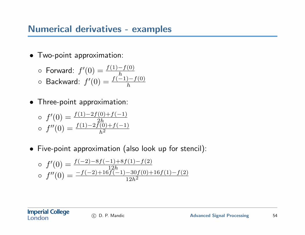
Numerical derivatives - examples

• Two-point approximation:

◦ Forward: f ′(0) = f(1)−f(0)h

◦ Backward: f ′(0) = f(−1)−f(0)h

• Three-point approximation:

◦ f ′(0) = f(1)−2f(0)+f(−1)2h

◦ f ′′(0) = f(1)−2f(0)+f(−1)h2

• Five-point approximation (also look up for stencil):

◦ f ′(0) = f(−2)−8f(−1)+8f(1)−f(2)12h

◦ f ′′(0) = −f(−2)+16f(−1)−30f(0)+16f(1)−f(2)12h2


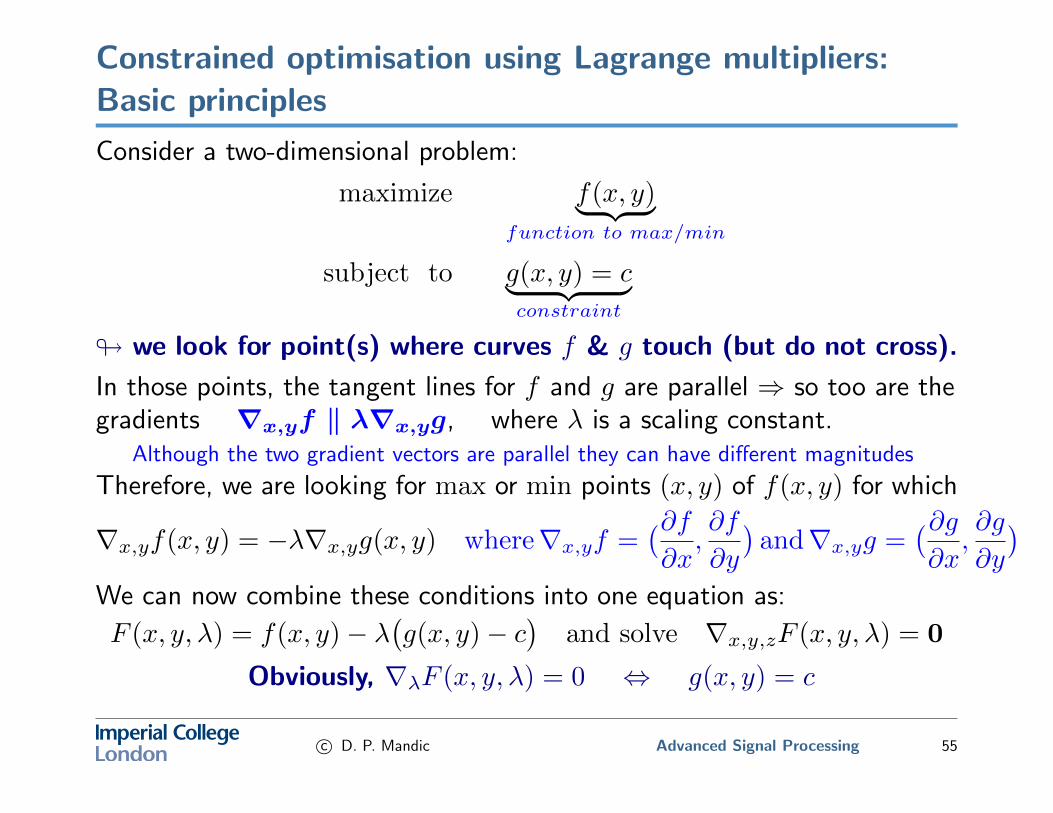
Constrained optimisation using Lagrange multipliers:Basic principles

Consider a two-dimensional problem:

maximize f(x, y)︸︷︷︸function to max/min

subject to g(x, y) = c︸︷︷︸constraint

# we look for point(s) where curves f & g touch (but do not cross).

In those points, the tangent lines for f and g are parallel ⇒ so too are thegradients ∇x,yf ‖ λ∇x,yg, where λ is a scaling constant.

Although the two gradient vectors are parallel they can have different magnitudes

Therefore, we are looking for max or min points (x, y) of f(x, y) for which

∇x,yf(x, y) = −λ∇x,yg(x, y) where∇x,yf =(∂f∂x,∂f

∂y

)and∇x,yg =

(∂g∂x,∂g

∂y

)We can now combine these conditions into one equation as:

F (x, y, λ) = f(x, y)− λ(g(x, y)− c

)and solve ∇x,y,zF (x, y, λ) = 0

Obviously, ∇λF (x, y, λ) = 0 ⇔ g(x, y) = c


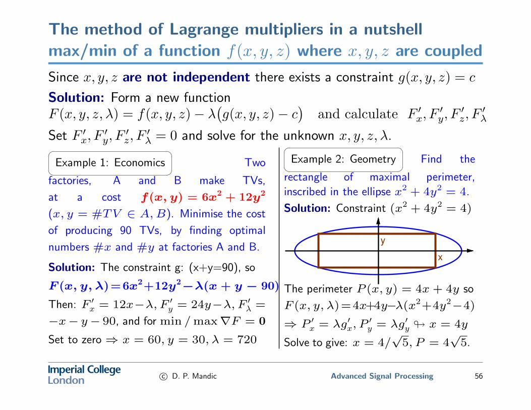
The method of Lagrange multipliers in a nutshellmax/min of a function f(x, y, z) where x, y, z are coupled

Since x, y, z are not independent there exists a constraint g(x, y, z) = c

Solution: Form a new functionF (x, y, z, λ) = f(x, y, z)− λ

(g(x, y, z)− c

)and calculate F ′x, F

′y, F

′z, F

′λ

Set F ′x, F′y, F

′z, F

′λ = 0 and solve for the unknown x, y, z, λ.�

�� Example 1: Economics Two

factories, A and B make TVs,

at a cost f(x, y) = 6x2 + 12y2

(x, y = #TV ∈ A,B). Minimise the cost

of producing 90 TVs, by finding optimal

numbers #x and #y at factories A and B.

Solution: The constraint g: (x+y=90), so

F (x, y, λ)=6x2+12y2−λ(x + y − 90)

Then: F ′x = 12x−λ, F ′y = 24y−λ, F ′λ =

−x− y− 90, and for min /max∇F = 0

Set to zero⇒ x = 60, y = 30, λ = 720

��

� Example 2: Geometry Find the

rectangle of maximal perimeter,

inscribed in the ellipse x2 + 4y2 = 4.

Solution: Constraint (x2 + 4y2 = 4)

y

x

The perimeter P (x, y) = 4x+ 4y so

F (x, y, λ)=4x+4y−λ(x2+4y2−4)

⇒ P ′x = λg′x, P′y = λg′y # x = 4y

Solve to give: x = 4/√5, P = 4

√5.


Notes:

◦


advanced signal processing lecture 1: random …mandic/asp_slides/asp_lecture_1_slides... ·...

Documents