advanced rank/select data structures: succinctness, bounds, and
TRANSCRIPT

Universita degli Studi di Pisa
Dipartimento di InformaticaDottorato di Ricerca in Informatica
Settore Scientifico Disciplinare: INF/01
Ph.D. Thesis
Advanced rank/select data structures:
succinctness, bounds, and applications
Alessio Orlandi
Supervisor
Roberto Grossi
Referee
Veli Makinen
Referee
Gonzalo Navarro
Referee
Kunihiko Sadakane
December 19, 2012


Acknowledgements
This thesis is the end of a long, 4 year journey full of wonders, obstacles, aspirations
and setbacks. From the person who cautiously set foot in Pisa to the guy who left
his own country, none of these steps would have been possible without the right
people at the right moment, supporting me through the dark moments of my life
and being with me enjoying the bright ones.
First of all, I need to thank Prof. Roberto Grossi, who decided that he could
accept me as a Ph.D. Student. Little he knew of what was ahead :). Still, he bailed
me out of trouble multiple times, provided invaluable support and insight, helping
me grow both as a person and as a scientist. I also owe a lot to Prof. Rajeev Raman,
who has been a valuable, patient and welcoming co-author. I also want to thank
Proff. Sebastiano Vigna and Paolo Boldi, who nurtured my passion for computer
science and introduced me to their branch of research. Also Prof. Degano, as head
of the Ph.D. course, provided me with non-trivial help during these years.
In Pisa, I met a lot of interesting people who were crucial for my happiness, was
it when studying on a Sunday, on a boring the-proof-does-not-work-again day, in
moments of real need, or on a Saturday night. Hence, this goes to Matteo S., Claudio
G., Rachele, Petr, Rui, Anna and Valentina M., Maddalena, Dario F., Andra, Carlo
de S., Rossano and Igor. And of course, I cannot forget my office mates, Giovanni
and Giuseppe, who provided valuable lessons of Sicilian and managed not to kill me
because of the open door.
Also, the last year has been full of changes and important steps in my life. I
doubt this thesis would never have been printed if it weren’t for you, Cristina, Niamh,
Mihajlo, Nicolas, Fred, Claudio, Andrea, Beatrice, Ivo. You guys know what I am
talking about.
Beyond this, I need to thank my family, whose love and support provided me with
the help one need when facing the unknowns of almost 4 years as a grad student.
I want to end by saying that it is hard to find people who have the bravery to
believe in you, to enjoy your life with, to trust you, to share the little triumphs, the
big losses, the hard lessons as well a laugh on the sunset on the beach, the kindness

4
of a tear, or the inspiration and the passion that drives you through. And I find it
even harder to let go those people the way I knew them. So, Mauriana, Fabrizio,
this “conclusion”, this thesis, is dedicated to you.

Contents
1 Introduction 9
1.1 Succinct data structures . . . . . . . . . . . . . . . . . . . . . . . . . 10
1.1.1 Systematic vs. non systematic . . . . . . . . . . . . . . . . . . 11
1.2 Thesis structure . . . . . . . . . . . . . . . . . . . . . . . . . . . . . . 12
1.2.1 Focus . . . . . . . . . . . . . . . . . . . . . . . . . . . . . . . 12
1.2.2 Motivation . . . . . . . . . . . . . . . . . . . . . . . . . . . . . 13
1.2.3 Contents . . . . . . . . . . . . . . . . . . . . . . . . . . . . . . 14
2 Basic concepts 19
2.1 Time complexities . . . . . . . . . . . . . . . . . . . . . . . . . . . . . 19
2.2 Space occupancy . . . . . . . . . . . . . . . . . . . . . . . . . . . . . 21
2.2.1 Empirical entropy . . . . . . . . . . . . . . . . . . . . . . . . . 21
2.3 Information-theoretic lower bounds . . . . . . . . . . . . . . . . . . . 22
2.4 Succinct bounds . . . . . . . . . . . . . . . . . . . . . . . . . . . . . . 24
2.5 On binary rank/select . . . . . . . . . . . . . . . . . . . . . . . . . . 25
2.5.1 Elias-Fano scheme . . . . . . . . . . . . . . . . . . . . . . . . 26
2.5.2 Relations with predecessor problem . . . . . . . . . . . . . . . 28
2.5.3 Weaker versions . . . . . . . . . . . . . . . . . . . . . . . . . . 30
2.5.4 Basic employment and usage . . . . . . . . . . . . . . . . . . . 32
2.6 Operating on texts . . . . . . . . . . . . . . . . . . . . . . . . . . . . 38
2.6.1 Generic rank/select . . . . . . . . . . . . . . . . . . . . . . . . 38
2.6.2 Compressed text indexing . . . . . . . . . . . . . . . . . . . . 39
2.6.3 Burrows-Wheeler Transform . . . . . . . . . . . . . . . . . . . 40
2.6.4 Backward search . . . . . . . . . . . . . . . . . . . . . . . . . 42
2.6.5 A more generic framework . . . . . . . . . . . . . . . . . . . . 43
3 Improving binary rank/select 45
3.1 Our results . . . . . . . . . . . . . . . . . . . . . . . . . . . . . . . . 45
3.2 Relationship with predecessor search . . . . . . . . . . . . . . . . . . 46
3.3 Searching the integers . . . . . . . . . . . . . . . . . . . . . . . . . . 49

6 CHAPTER 0. CONTENTS
3.3.1 Previous work: searching in O(log log u) time . . . . . . . . . 49
3.3.2 Previous work: searching in o(log n) time . . . . . . . . . . . . 50
3.3.3 New result: searching systematically . . . . . . . . . . . . . . 51
3.4 An improved data structure . . . . . . . . . . . . . . . . . . . . . . . 53
3.4.1 Overview of our recursive dictionary . . . . . . . . . . . . . . 53
3.4.2 Multiranking: Oracle ψ . . . . . . . . . . . . . . . . . . . . . . 55
3.4.3 Completing the puzzle . . . . . . . . . . . . . . . . . . . . . . 57
3.4.4 Proof of main theorems . . . . . . . . . . . . . . . . . . . . . . 58
3.5 Density sensitive indexes . . . . . . . . . . . . . . . . . . . . . . . . . 60
3.5.1 Preliminary discussion . . . . . . . . . . . . . . . . . . . . . . 60
3.5.2 A succinct index for rank/select1 . . . . . . . . . . . . . . . 61
3.5.3 A succinct index for select0 . . . . . . . . . . . . . . . . . . . 62
4 Rank and select on sequences 65
4.1 Our results . . . . . . . . . . . . . . . . . . . . . . . . . . . . . . . . 65
4.2 Related work . . . . . . . . . . . . . . . . . . . . . . . . . . . . . . . 67
4.3 Extending previous lower bound work . . . . . . . . . . . . . . . . . . 67
4.4 A general lower bound technique . . . . . . . . . . . . . . . . . . . . 72
4.5 Proof of Theorem 4.2 . . . . . . . . . . . . . . . . . . . . . . . . . . . 77
4.5.1 Encoding . . . . . . . . . . . . . . . . . . . . . . . . . . . . . 79
4.6 Upper bound . . . . . . . . . . . . . . . . . . . . . . . . . . . . . . . 83
4.6.1 Bootstrapping . . . . . . . . . . . . . . . . . . . . . . . . . . . 83
4.6.2 Supporting rank and select . . . . . . . . . . . . . . . . . . 84
4.7 Subsequent results . . . . . . . . . . . . . . . . . . . . . . . . . . . . 86
5 Approximate substring selectivity estimation 89
5.1 Scenario . . . . . . . . . . . . . . . . . . . . . . . . . . . . . . . . . . 89
5.2 Preliminaries . . . . . . . . . . . . . . . . . . . . . . . . . . . . . . . 91
5.2.1 Suffix trees . . . . . . . . . . . . . . . . . . . . . . . . . . . . 91
5.2.2 Pruned suffix trees . . . . . . . . . . . . . . . . . . . . . . . . 92
5.2.3 Naive solutions for occurrence estimation . . . . . . . . . . . . 93
5.2.4 Previous work . . . . . . . . . . . . . . . . . . . . . . . . . . . 94
5.3 Uniform error range . . . . . . . . . . . . . . . . . . . . . . . . . . . . 95
5.4 Lower-side error range . . . . . . . . . . . . . . . . . . . . . . . . . . 100
5.4.1 Computing counts . . . . . . . . . . . . . . . . . . . . . . . . 101
5.4.2 Finding the correct node . . . . . . . . . . . . . . . . . . . . . 102
5.5 Lower bounds . . . . . . . . . . . . . . . . . . . . . . . . . . . . . . . 106
5.6 Experiments . . . . . . . . . . . . . . . . . . . . . . . . . . . . . . . . 107

0.0. CONTENTS 7
6 Future directions 113
Bibliography 115

8 CHAPTER 0. CONTENTS

Chapter 1
Introduction
Analysis and manipulation of large data sets is a driving force in today’s development
of computer science: information retrieval experts are pushing against the limits
of computation capabilities and data processing every day, both in academic and
industrial environment. The data to process can be expressed in different formats:
unstructured text, semi-structured data like HTML or XML, fully structured data
like MIDI files, JPEG images, etc.. Data can be simply stored in some format, to
be retrieved afterward, processed by a huge amount of machines in parallel that
simply read it, manipulated to be altered, or searched, . . . Searching is, indeed, one
of the most fascinating challenges: from simply retrieving to semantic interpretation
of documents current computer science is employing massive data set computations
to provide universal access to information (see e.g. http://www.wikipedia.org or
http://www.yahoo.com).
At a design level, this translates into a set of less or more complex analyses and
re-encoding of the collection documents (see e.g. [WMB99, BYRN11]) in a more
suitable fashion so that retrieval can be eased. There are, then, multiple scenarios
having a number of fixed points in common:
• Data is heterogeneous, but is usually naturally unstructured or semi-structured
text (searching on images is a completely different area).
• Data is large, but is highly compressible: (un)structured text is still a predom-
inant category of data sources and there exist a lot of compressors explicitly
designed for it
• Data is static: when dealing with massive data sets, keeping data static is a
great simplification both for compression, handling and testing reasons.
Compression is then a tool with multiple effects: by occupying less space, it is
more economical to store data; moreover, it helps transforming network- and I/O-

10 CHAPTER 1. INTRODUCTION
bound applications into CPU-bound ones. Compressed data can be read and fed to
the CPU faster and, if it the compression ratio is particularly effective, can lead to
entire important chunks of data to be entirely in cache, speeding up computations
and outweighing the processing penalty of decompression. As an extreme nontrivial
example one can think of the LZO1x algorithm [LZO] that has been used to speed
up transmission between Earth and the NASA Spirit and Opportunity rovers. They
claim performance of 3× speed slowdown w.r.t. in-memory-copy for decompression
at an average text compression of 2.94 bits/byte, i.e. bringing the file size to almost
1/3 of its original size. Compressed data was then used in soft and hard real-time
computations on the rovers, proving almost flawlessly transparent to underlying
computation, also in terms of memory and CPU consumption.
Back to the original example, after an initial warehousing phase, analysis and
serving systems, or just databases, need to access the underlying data. Traditionally
this involves locating the chunk of data to load, decompressing it and operating
on it, implying that computations repeated intensively on compressed data can
cumulatively bring the balance of enforcing compression on the negative side. A
solution to the dilemma is compressed data structures, and algorithms running on
those: when the set of operations to be performed on the compressed data is stated
in advance, compression may be tweaked so that operations can be performed on the
data without actually decompressing the whole stream but just the areas of data that
are interested by the specific query. In a sense, these data structure operate directly
on the compressed data. Compressed data structures evolved into an entire branch
of research (see bibliography), especially targeting the most basic data structures –
the rationale behind it being that the more basic the data structures the more likely
they are involved in any computation – and mainly binary and textual data.
1.1 Succinct data structures
Compressed data structures usually work as follows: the data is initially compressed
with an adhoc compression mechanism. Then, a little amount of additional data
must be introduced to perform the necessary data structure operation on the un-
derlying data. Hence, the space complexity of compressed data structures is divided
in a first, data-only, measure, plus a redundancy additional factor, which usually
depends on the time requested to perform the data structure operation. A specific
and well studied class of compressed data structures is called succinct data struc-
tures, the term succinct meaning that, under a certain data model, the redundancy
footprint is a lower-order term of the data-only measure. As a matter of fact if a
string requires b bits to be represented at least, then a succinct data structure will

1.1. SUCCINCT DATA STRUCTURES 11
use o(b) additional bits to perform the requested operations. A more thorough ex-
planation of succinct bounds, being the principal focus of this thesis, can be found
in Section 2.2.
1.1.1 Systematic vs. non systematic
Data structures are divided into two main categories: systematic and non-systematic
ones [GM07]. Many classical data structures are non-systematic: given an object c,
the data structure can choose any way to store c, possibly choosing a representation
helping the realization of a set of operations Π with low time complexity. Systematic
data structures are different since the representation of the data cannot be altered;
it is hypothesized that access to the data is given by an access operation that the
succinct data structure uses to probe the data. The semantics of access depends
on the current data domain. For example, considering strings in the character RAM
model, access(i) refers to the ith character of the input string. The additional
data that systematic data structures employ to perform their task is referred to as a
succinct index, as it is used to index the original data and at the same time must not
exceed the succinct bound, namely the index must be lower order term of the data
size. A data structure that receives a string and encodes it as-is, providing search
for any substring P into the string by just scanning, is a systematic data structure.
A data structure encoding the input string by just rearranging the characters so as
to ease search, is a non-systematic one.
Given their traits, comparing systematic and non-systematic succinct data struc-
tures is intrinsically difficult: data for systematic ones can be stored in any format,
hence the only space complexity to be held into account is the redundancy, i.e. the
amount of redundancy used to support operations, whereas non-systematic ones op-
erate differently. In the latter case, there can be no conceptual separation between
data encoding and index size. For example, let f(n, σ) be the minimum information-
theoretic space needed to store a string of length n over an alphabet of size σ. Let
also π denote a set of operations to be supported on strings. A non-systematic
data structure that can store strings in f(n, σ) + O(n/ log σ) bits while providing
π can be, overall, smaller or larger than a systematic data structure with the same
redundancy of O(n/ log σ) bits: depending on how S is kept encoded, an O(f(n, σ))
data structure providing access to the string instead of a plain n log σ bits encoding
would pose a difference.
Both approaches have advantages and drawbacks: a non-systematic data struc-
ture is in control of every aspect of the data, and by exploiting its best representation
w.r.t. the operations to be performed, can as such outperform a systematic one in
terms of space complexity. Clearly, this solution can be employed only if the data
12 CHAPTER 1. INTRODUCTION
can be re-encoded by the data structure for its own purposes, discarding the original
representation. On the other hand, consider two sets of operations Π1 and Π2 to
be implemented on the same object c, so that no single non-systematic data struc-
ture implementing both exists: the solution with non-systematic data structures is
to store the data twice, whereas systematic ones can exploit their indirect relation
with data to provide, in some scenario, a better result.
Finally, separation of storage and operations can help in more complex environ-
ments. It is not uncommon that the basic object representation of c to be multiple
times larger than the index itself, so that in some scenarios storage of the data itself
onto the main memory is prohibitive, even in a transparently compressed format
that the data structure does not control. Whereas the index can be loaded into
main memory, the data must be accessed through on-disk calls. The modularity of
systematic succinct data structures comes into help: data structures can be designed
so as to minimize usage of the access primitive and work very well in such models.
1.2 Thesis structure
1.2.1 Focus
In this thesis, we focus our attention on studying, creating and applying one of
the most prominent subclasses of succinct data structures, both in systematic and
non-systematic fashion, called rank and select data structures. Operations are
performed on strings of the alphabet [σ] = 0, 1, 2, . . . , σ − 1, where σ ≥ 2. For a
string S = [0, 1, . . . |S| − 1] of length n, the data structure answers to two queries:
• rankc(p), for c ∈ [σ], p ∈ [n + 1], which returns1 |x < p|S[x] = c|, i.e. the
number of characters of value c present in the prefix of p characters of S.
• selectc(i), for c ∈ [σ], i ∈ [1, n] which returns the position of the ith-most
occurrence of c in S from the left from the left, namely returns y such that
S[y] = c and rankc(y) = i− 1, or −1 if such position is nonexistent.
For example for S = abcbbca, rankb(3) = 1 and selectc(1) = 2, while selectc(3) =
−1. Furthermore, for2 S = 0110101 we have rank1(3) = 2 and select0(1) = 0.
1In literature, sometimes the definition x ≤ p|S[x] = c is preferred, although it easily create
inconsistencies unless the string is indexed from 1.2To avoid confusion, we use 0 and 1 to denote characters in binary strings

1.2. THESIS STRUCTURE 13
1.2.2 Motivation
There are a number of high level motivations for this thesis to focus on rank and
select data structures. We now give a less technical overview and motivation for the
whole thesis. Chapter 2 gives a more detailed and technical overview. Section 1.2.3
gives a per-chapter motivation to the results in the thesis.
First, they are basic operations in computer science. If one considers the binary
case, where σ = 2, performing select1(rank1(x)) for some x recovers the predecessor
of x, i.e. maxyy < x, S[y] = 1. To grasp the importance of this operation, let us
consider a set of IPv4 net addresses, say 1.1.2.0, 1.1.4.0, etc. The basic operation
in a router is to perform routing lookup: given a destination IP address, say 1.1.2.7,
find the network address that matches it, by finding the IP address with the longest
common prefix with it. Not surprisingly, this can be reduced to a set of predecessor
searches: let us interpret IPv4 address as 1s in a string of 232 bits. Finding the
predecessor of the 32-bit representation of the destination IP address, gives the
possible next hop in routing. In a sense, predecessor problem is one of the most
diffused and executed on the planet. Since storing routing tables compactly while
keeping fast predecessor lookup is important [DBCP97], study of rank and select
operations is well justified, both in theory and in practice.
Still in the binary case, rank and select are relevant without the need to be
combined into predecessor search. For select a simple idea is given by the following
scenario. Let us consider a static set of variable length records R0, R1, . . . , Rn−1.
Those records can be stored contiguously, with the caveat that it would make difficult
to have random access to each record. Assuming the representation of all records
requires u bits, one can store a bitvector of u bits with n 1 inside, marking the
bit that denotes the start of the record. Performing select1(k) for some k gives
the address at which the kth record begins [Eli74a, Fan71a]. This would require
n log(u/n) +O(n) bits to be encoded by means of simple schemes, and select can
be solved in O(1) time. Considering that the trivial O(1)-time solution of array of
fixed-size pointers would require nw bits (where w is the size of the pointer), and
we can assume w.l.o.g. that u ≤ nw, the difference is self-evident: n log(u/n) ≤n logw nw, for w larger than some constant.
For rank operation, consider again the set of IPv4 addresses as 32 bits values.
Assume that for a subset of those IP addresses, some satellite data has to be stored.
To be practical, assume that the physical network interface to reach that address is
to be added (so that we have a small integer). Hence, we assume that we have a
universe of u = 232 values out of which n values are selected to be decorated with the
satellite data. One can encode a bitvector B of u bits with n ones, setting B[i] = 1
iff the ith IP address has some satellite data attached. Then, one can encode B

14 CHAPTER 1. INTRODUCTION
and lay down the satellite data for each record in a consecutive array C so that the
C[rank1(i)] is the data attached to the ith IP, since rank1(i) over B will retrieve
the rank (in the mathematical sense) of the ith IP among those selected.
rank and select data structure are bread and butter of other succinct data
structures. For the binary case, it turns out [Jac89, MR01] that they are the basic
tool to encode static binary trees: given a tree of n nodes, rank and select data
structures are the basic piece to obtain a representation of 2n + o(n) bits which
supports a wide variety of navigation operations (up to LCA and Level ancestors)
in constant time.
For the generic alphabet case, they are at the basis of compressed text index-
ing [GV05, Sad03, ?]: given a text T , it is possible to compress it and at the same
time search for occurrences of arbitrary patterns in T . The data structures have
necessarily to spend more space than the simple compression, but the resulting ad-
vantage is substantial: instead of having to decompress the whole text to perform
substring searching, the text can be decompressed only in “local” regions which are
functional to the substring search.
rank and select have also a complex history. Being intertwined with prede-
cessor data structures, they received indirect and direct attention in terms of lower
bounds. This is especially true for the binary case. Various studies [Gol07b, Ajt88,
BF02, PT06b, PV10] proved that there exist separation barriers on the minimum
time complexity for predecessor search as a function of the space used by the data
structure, the universe size and the word size of the machine we operate on. As
a result, multiple paths have been taken: some researchers insisted on O(1) time
complexity and small spaces when both are possible; others tried to focus on fast
systematic data structures irrespective of the space complexities; others explored
small, although non-optimal, space complexities giving up on the constant time.
Finally, rank and select data structures have been studied in practice, proving
that some schemes are actually interesting, or can be engineered to be, in practical
scenarios [GGMN05, GHSV06, OS07, Vig08, CN08, OG11, NP12].
1.2.3 Contents
The thesis is structured as follows.
Basic concepts
Chapter 2 contains a more thorough introduction to succinct data structures in
general, providing an overview of related work, applications and past relevant results
in the world of such data structures. The chapter also serves as an introduction

1.2. THESIS STRUCTURE 15
to many of the data structures that will use as comparison or as pieces in our
constructions in the chapters to follow.
Improving binary rank/select
Chapter 3 contains the first contributions about binary rank/select data structure,
introducing a data structure able to operate in little space where it was not possible
before. The results were originally presented in [GORR09] and [GORR12] (preprint
available as [GORR11]).
Given a universe U of size u = |U | and a subset X ⊆ U of size n = |X|, we
denote by B(n, u) the information-theoretic space necessary to store X.
Among non-systematic data structures, multiple results been presented in the
past. If one assumes that u ≤ n logO(1) n, it is possible store X in B(n, u) +
o(n) bits maintaining O(1) rank time complexity. On that line, Pagh [Pag01] ob-
tained B(n, u)+O(n log2 log u/ log u). Afterwards, Golynski et al. [GRR08] obtained
B(n, u) +O(n log log u log(u/n)/ log2 u). An optimal solution in this dense case was
proved by Patrascu [P08], obtaining, for any t > 1,
B(n, u) +O
(utt
logt u
)+O
(u3/4 logO(1) u
),
with O(t) time to execute rank, essentially closing the problem (see [PV10] for a
proof). For sparser cases, namely when u = ω(n logO(1))n, Ω(n) bits of redundancy
are necessary [PT06b, PV10] for O(1) rank. To keep this time complexity Golyn-
ski et al. [GGG+07] obtained B(n, u) + O(u log log u/ log2 u) bits. Note that also
Patrascu’s data structure can be applied to the sparse case, still being a competitive
upper bound.
We introduce a novel data structure for the sparser case. Let s = O(log log u)
be an integer parameter and let 0 < δ, ε ≤ 1/2 be two parameters. Also recall that(B(n,u)=logdu
ne
). Theorem 3.1 shows how to store X in
B(n, u) +O(n1+δ + n log log u+ n1−sεuε)
bits of space, supporting select and rank operations in O(log(1/(δsε))) time. Sim-
ilarly, under the additional assumptions that s = Θ(1) and u = O(n2logn/ log logn)
Theorem 3.2 shows how to store X in
B(n, u) +O(n1+δ + n1−sεuε)
bits of space supporting rank and select in O(log(1/(δε))).
In particular, Theorem 3.2 surpasses Patrascu’s solution for δ = O(1/ log n)
range, since his data structure is optimal for the denser cases. Theorem 3.1 has a

16 CHAPTER 1. INTRODUCTION
different role: it proves that already existing data structures for predecessor search
(hence tightly connected to rank1) can be employed to support select0 (a non-
trivial extension) without the need to actually write the complement of X, which
may be quite large.
Rank and select on sequences
Chapter 4 contains contributions about systematic data structures, proving an opti-
mal lower bound for rank and select strings. The results were originally presented
in [GOR10].
In this scenario, we assume to have a string S of length n over alphabet [σ]
that we can probe for each character, so that access(i) = S[i] for any 0 ≤ i <
|S|. We study systematic data structures for rank and select over S. These
data structures where, up to our work, limited to rank in ω(log log σ) time, when
o(n log σ) bits of redundancy were used. Regarding the binary case, a clear lower
bound for systematic data structures was proved by Golynski [Gol07a], so that for
any bitvector of length u, in order to execute rank and select with O(t) calls to
access for single bits of the bitvector, an index must have Ω(u log log(t log u)t log u
) bits of
redundancy. No lower bound for the generic case was available. At first, one could
be tempted to just generalize the techniques of the binary case to the generic case.
This actually leads to a lower bound of Ω(n log tt
) bits for O(t) calls to access, as
proved by our Theorem 4.1 which is extremely weak when t = o(σ). Indeed, a linear
trade off for systematic data structures on strings was already proved by Demaine
and Lopez-Ortiz [DLO03]. Our Theorem 4.3 and Theorem 4.4 finally prove that for
any t = o(log σ), a redundancy of r = Ω(n log σt
) bits of redundancy are necessary for
either rank and select, independently.
Assuming ta represents the time to access a character in the representation of the
string S on which the data structure is built, Barbay et al. [BHMR07c] gave a data
structure able to perform rank in O(log log(σ) log log(σ)(ta + log log σ)) time with
O(n log σlog log σ
) bits of redundancy. In terms of number of calls to access, the complex-
ity amounts to O(log log σ log log log σ). They can perform select in O(log log σ)
calls to access and O(ta log log2 σ) total time. The indexes of [BHMR07c] can also
be squeezed into entropy bounds, providing a data structure that performs on highly
compressed strings.
Our Theorem 4.6 proves that for any fixed t = O( log σlog log σ
) one can build an in-
dex in O((n/t) log σ) bits that (i) solves selectin O(tat) time and O(t) probes (ii)
solves rank O(t(ta + log log σ)) time and O(t) probes. Hence, we prove that with
O(n log σlog log σ
) extra bis, one can do rank in exactly O(log log σ) time. This means
that, in term of calls to access, as long as t = o(log σ/ log log σ), our data struc-

1.2. THESIS STRUCTURE 17
ture is optimal. We also provide, in Corollary 4.2, a way to compress both the
original string and our data structure in very little space. Moreover, subsequent
studies [BN11a] shows that, within those space bounds, O(log log σ) is the optimal
time complexity to execute rank and select on strings with large alphabets, namely
when log σ/ logw = O(log σ)).
Approximate substring selectivity estimation
Chapter 5 contains a novel application of rank and select data structures to ap-
proximately count the number of occurrences of a substring.
Given a text T of length n over alphabet [σ], there exist many data structures for
compressed text indexing that can compress T and allow for substring search in the
compressed version of T : given any pattern P such data structures are able to count
the exact number of occurrences of P inside T . Not all applications require the exact
count; for example, the selectivity estimation problem [JNS99] in databases requires
only an approximate counting of pattern occurrences to perform efficient planning
for query engines. More formally, given a fixed value l ≤ 1, if y = Count(P ) is the
actual occurrence count for P , we expect to give an answer in [y, y + l − 1].
The database community provided multiple results [JNS99, KVI96, LNK09,
CGG04, JL05] aimed mainly at practical speed. We perform the first theoreti-
cal and practical study strictly regarding space efficiency. We study the problem in
two variants: the uniform error range, where we answer within [y, y+ l − 1] for any
pattern P , and the lower-sided error range, where for any pattern that occurs more
than l times in T , the count is actually correct.
We initially extend existing results in compressed text indexing to prove in Theo-
rem 5.2 that, for l = o(σ), an index for the uniform error case can be built in optimal
Θ(|T | log σl
) bits. The time complexity depends on the underlying rank/select data
structure for strings that is chosen at construction time.
We also provide a solution for the lower sided error range based on pruned suffix
trees. It is not easy to immediately state the space occupancy of our data structure,
which scales with the amount of patterns that appear more than ` times in the text.
We refer the reader to Theorem 5.4 for details.
Finally, Section 5.6 rejoins our results with the original works of selectivity esti-
mation. For comparison, we give the average error measured on a number of random
patterns, provided that previously known data structures and our data structure
match in space occupancy. As a result, we have cases in which the average error is
always less than 2.5, even when we set l = 32. This gives improvements up to 790
times with respect to previous solutions.

18 CHAPTER 1. INTRODUCTION

Chapter 2
Basic concepts
This chapter recalls some fundamental techniques and concepts used throughout
the rest of this thesis. A first part describes the very basic notation, including
the computational model into which we deliver our work and how succinct data
structures are categorized. Next, we describe data structures that are connected to
the original results presented in forthcoming chapters.
Throughout the whole thesis, we will refer to logarithms as in base 2, that
is, log x = log2 x. To ease readability, we define log(1) x = log(x) and log(i) x =
log log(i−1) x for i > 1 and we use the notation logk f(x) as a shortcut for log(f(x))k
for any k and f(·). Finally, we will often use forms similar to log(x)/y. To ease read-
ability, we will omit parentheses, writing them as log x/y, so that log x/ log log(1/x)
is actually log(x)/ log log(1/x) for example.
We also recall the definition of O: f(x) is said to be O(g(x)) if f(x) isO(g(x)polylog(x)).
2.1 Time complexities
Data structures and algorithms can exploit the specific computational model they
operate on. As such, they are also subject to specific time lower bounds. Some
models are more abstract (like the bit-probe model), some are more realistic (e.g.,
Word-RAM) and some are tightly related to lower bounds (cell-probe model). We
now describe the ones that will be used throughout the thesis.
Word RAM model
The Word Random Access Machine is a very realistic model, i.e., it tries to model a
physical computer, where a CPU executes 1 the algorithm step by step and accesses
1Here we refer to the basic AC0 operations, plus multiplication

20 CHAPTER 2. BASIC CONCEPTS
locations of memory in a random fashion in O(1) time (this is in contrast to the
classic Turing machine with sequential access). The model relies on the concept
of word : a contiguous area of memory (or working memory inside the CPU) of
w bits, for some parameter w. The memory is organized in contiguous words of
w bits. When computing time complexities, single accesses to a word costs O(1)
time units. Every elementary mathematical and logical operation takes effect on a
constant number of words in O(1) time. It is usually assumed that the Word RAM
is trans-dichotomous : supposing the problem has a memory size driven by some
value n, it holds that w ≥ log n . Note that a non-trans-dichotomous RAM would
not be able to address a single cell of the data structure using w < log n bits.
Cell probe model
The classic cell probe model, introduced by Yao [Yao81], is the usual environment into
which lower bounds for the Word RAM model are proved. The model is exactly the
same, however, the computational cost of an execution is given by the sole number
of probes executed over the memory. In other words, the cell probe model is a word
RAM model where the CPU is arbitrarily powerful, in contrast to being limited to
basic mathematical and logical operations.
Bit probe model
The bit probe model is a model based on the assumption that a random access
memory of finite size exists and the algorithm may perform single bit probes. More
formally, a CPU exists and an algorithm may perform elementary mathematical and
logical operations plus accessing one single bit of memory in O(1) time. Computa-
tional time is computed by summing the time of elementary operations and accesses
to memory. In other words, it is the cell probe model, with w = 1.
The bit probe model can also be used to prove lower bounds, where only the
amount of memory accesses is considered.
Character RAM model
A variation over the Word RAM model is the character RAM model, which we for-
mally introduce in this thesis. It is defined by two parameters: σ (alphabet size,
bits) and w (word size). The CPU works as in the Word RAM model, with opera-
tions over entire words, and it is supposed to be trans-dichotomous. The memory
is instead divided into two different areas: a data and an index area. Accesses to
the data area are limited to contiguous area of log σ bits each, performed through a
specific access(·) call, instead of w bits as in the Word RAM model. Accesses to the

2.2. SPACE OCCUPANCY 21
index are of normal word size. The time complexity here is provided by the number
of probes in the data area, plus the probes in the index area, plus the computation
time. The character RAM model is a good approximation of communication-based
models, where access to the underlying data is abstract and is designed to retrieve
the logical unit of information (i.e., the character).
The character probe model is a hybrid between the cell probe model and the
character RAM model: the machine has an index memory (which may be initialized
with some data structure) and every computation done with such index memory
is completely free. The only parameter of cost is the number of access-es to the
underlying data, which are character-wide. In other words, it is the character RAM
model where the cost for index computations is waived. This model was already
used in [Gol07b].
2.2 Space occupancy
2.2.1 Empirical entropy
Shannon’s definition of entropy [CT06] can be given as follows:
Definition 2.1. Given an alphabet Σ, a source X is a discrete random variable over
Σ, whose probability density function is denoted by p(·). Its entropy is defined as
H(X) =∑c∈Σ
p(c) log 1/p(c).
Shannon’s entropy [CT06] is tightly connected to compression, as it defines how
easy to compress is a probabilistic source. As all generic definitions, it is acceptable
when no further knowledge is available. It can be used to deduce the compressibility
of distributions as a whole. On the other hand, from one factual output of the source,
it is impossible to use Shannon’s entropy to bound the compressibility the output
text.
In recent years [Man01] empirical entropy has shown to be a powerful tool in
the analysis of compressors performance, overcoming the limitation of Shannon’s
entropy. At a high level the definition of entropy starts from the text output of an
unknown source:
Definition 2.2. Given a text T over an alphabet Σ of size σ, let nc be the number
of occurrences of c in T and let n = |T |. Then, the zero-th order empirical entropy
of T is defined as
H0(T ) =1
n
∑c∈Σ
nc logn
nc

22 CHAPTER 2. BASIC CONCEPTS
Viewing the nc/n factor as an estimator of the probability of character c ap-
pearing in the text, we can assume T to be generated by a probabilistic source in
Shannon’s setting where p(c) = nc/n (note that we created the source onto the
specific text). Assume to have the text T and to build p(·) as described, then, the
Shannon’s entropy of the text is
H(T ) =∑c∈Σ
ncn
logn
nc,
hence proving the same definition. Therefore, the value nH0(T ) provides an information-
theoretic lower bound on the compressibility of T itself for any compressor that
encodes T by means of encoders that do not depend on previously seen sym-
bols [Man01]. An example of such encoder is Huffman’s coding (we assume the
reader familiar with the concept [CLRS00].
More powerful compressors can achieve better bounds by exploiting the fact
that when encoding/decoding a real string, some context is also known. Empirical
entropy can be extended to higher orders, exploiting the predictive power of contexts
in the input string. To help define kth order empirical entropy of T , for any string U
of length k, let UT be the string composed by juxtaposing single symbols following
occurrences of U in T . For example if T = abracadabra$ and U = ab, then Uab = rr,
as the two occurrences of ab in T are both followed by r. Then, the k-order entropy
of T is defined as:
Hk(T ) =1
n
∑U∈Σk
|UT |H0(UT ),
where Σk is the set of all strings of length k built with characters in Σ.
Empirical entropy has been intensively used [Man01] to build a theory explain-
ing the high performance of Burrows-Wheeler Transform based compressors (e.g.,
bzip2), since higher order entropies (k ≥ 1) always obey the relationship
Hk(T ) ≤ Hk−1(T ).
Burrows-Wheeler transform and its relation with empirical entropy are thoroughly
discussed in Section 2.6.3. More details about empirical entropy and the relation to
compressors can be found in [Man01].
2.3 Information-theoretic lower bounds
Given a class of combinatorial objects C, the minimum amount of data necessary
for expressing an object c ∈ C is log |C| bits, equivalent to the expression of entropy

2.3. INFORMATION-THEORETIC LOWER BOUNDS 23
in an equiprobable setting. This quantity is often called the information-theoretical
bound. Inasmuch log |C| poses a lower bound, it is not always a barrier. The first
strategy to avoid the limitation is to further refine class |C|, by introducing more
constraints on the data. If C is the class of all bitvectors of length u, then log |C| = u,
but if we can restrict to a subclass of C, say Cn of bitvectors of length u with n bit
set to 1, then log |Cn| = log(un
). This for bitvectors is widely used in literature since
it is, similarly to empirical entropy, a data aware measure.
Definition 2.3. Given a bitvector B of size u with cardinality n, the information
theoretical bound is
B(n, u) =
⌈log
(u
n
)⌉.
By means of Stirling inequality it is easy to see that
B(n, u) = n log(un
)+ (u− n) log
(u
u− n
)−O(log u)
The function is symmetric and has an absolute maximum for n = u/2, as B(u/2, u) =
u−O(log u), so that one can restrict to the case n ≤ u/2 and avoid considering the
remaining values, obtaining that
B(n, u) = n log(u/n) +O(n).
As one can see, for bitvectors, the information theoretical bound is equivalent, up
to lower order terms, to the empirical entropy bound: let B be a bitvector of u bits
with n 1s; then, for c = 1 we have n occurrences and for c = 0 we have u − n
occurrences. Substituting into Definition 2.2 gives that
H0(B) =n
ulog(un
)+u− nu
log
(u− nn
),
so that uH0(B) = B(n, u) +O(log u). In general, the information theoretical bound
is mainly used where more sophisticated methods of measuring compressibility are
not viable: higher order empirical entropy, for example, is suitable mainly for strings,
whereas trees and graphs have no affirmed compressibility measure.
Another example is given by the information theoretic limit used to represent
ordinal trees. An ordinal tree is a tree where children of a node are ordered, whereas
in a cardinal tree the ith child of a node is specified by explicitly specifying the
index i. For example, in a cardinal tree a node can have child 3 and lack child 1.
Many basic trees in computer science books are usually ordinal; cardinal trees are
frequently associated with labelled trees such as tries, or binary search trees. We
remark that, since there exists a bijection between binary cardinal trees and arbitrary

24 CHAPTER 2. BASIC CONCEPTS
degree cardinal trees, it is sufficient to have a lower bound over the representation
of binary trees to induce one over cardinal trees. The number of cardinal binary
trees of n nodes is given by the Catalan number Cn ' 4n/(πn)3/2 (see [GKP94] for
a proof), hence
Lemma 2.1. An ordinal tree of n nodes requires log Cn = 2n − Θ(log n) bits to be
described.
2.4 Succinct bounds
The concepts of entropy and information theoretical lower bound are vital for suc-
cinct data structures too. Consider a set Π of operations to be performed on any
object c, with some defined time complexity. Beyond the sole space occupancy for
c’s data, many data structures involve encoding additional data used to perform
operations on the representation of c itself. The space complexity of the data struc-
ture can be split into two parts: the information theoretical lower bound (log |C|bits) and the additional bits required to implement Π over c, usually referred to as
redundancy of the data structure. We assume the setting to be static: the data is
stored once and the operations do not modify the object or the index representation.
For example, consider the class CB of balanced bitvectors, having u bits of which u/2
are set to 1. Then, log |C| = log(uu/2
)= u−O(log u) bits. Suppose a data structure
must store C and providing operation count(a, b), returning the number of bits set
to 1 in the interval [a, b]. A data structure employing u + O(u/ log u) bits for that
has a redundancy of O(u/ log u) bits. Data structures can be classified with respect
to their size: data structures employing ω(log |C|) bits are standard data structures.
An example is the data structure that solves rank/select on a balanced bitvec-
tor B, with O(uw) bits: the data structures stores, in a sorted array, the value of
rank(i) for each i ∈ [u] and, in another sorted array, the value of select(j) for
each j such that Bj = 1. Data structures using O(log |C|) bits are called compact;
proper succinct data structures use log |C|+o(log |C|); finally, we have implicit data
structures that use log |C| + O(1) space. For succinct data structures, the quan-
tity log |C| + o(log |C|) is often referred to as the succinct bound. Among succinct
data structures, the smaller the redundancy for a fixed set of time settings for the
operations, the better the data structure.
In the dynamic setting, succinct data structures must maintain the succinct
bound among updates: after any update operation, at instant r, supposing the
description of the object requires log |Cr| bits, the data structure must maintain a
log(|Cr|)(1 + o(1)) occupancy rate.
For binary vectors, succinct rank/select data structures use B(n, u)+o(B(n, u))

2.5. ON BINARY RANK/SELECT 25
bits and, possibly, B(n, u) + o(n) when available. In the string setting, where n is
the string length and σ is the alphabet size, a succinct data structure will use
n log σ + o(n log σ) for any string S. It is easy to note that for the arbitrary string
the succinct bound is a more permissive definition. This is dictated by the presence
of certain lower bounds, which will be presented later.
Succinct bounds must also be seen in the logic of the data structure actual needs.
The class C of elements should be as much restricted as possible, constrained to the
minimum set of information that are actually needed to perform the operation. The
more those operations are data-independent, the smaller the bound becomes. An
important example is the data structure for Range Minimum Queries (RMQ) over
integer arrays developed by Fischer [Fis10]. The data structure allows one to create
an index that can answer RMQ over an array A of n integers as rmq(i, j) = z,
where i, j and, more importantly, z are indexes of positions in A. Considering the
data structure does not require to access A at all, it does not need to represent it.
Hence, the succinct bound to be compared with is not n log n (space to represent
A) but 2n−Θ(log n). The latter is given by the equivalence of RMQ and the need
to represent a Cartesian Tree shape over the elements of A, which requires, as per
Lemma 2.1, 2n−Θ(log n) bits at least.
2.5 On binary rank/select
This section explores some results and applications of basic rank and select data
structures in the binary case, excluding the results of the thesis.
Let us consider the Word RAM model with w-bit words and a universe set U
from which we extract a subset X. Here, |U | = u and |X| = n. We often refer to
n as the cardinality of X and to u as the universe (size). Note that we will often
change our point of view from the one of a bitvector to the one of a subset. This
is possible by a trivial, although important, duality where a bitvector B can be
interpreted as a subset:
Definition 2.4. Let B be a bitvector of length u of cardinality n. Let U = [u] be
called the universe. Then B can be interpreted as the characteristic function for
a (sorted) set X ⊆ U , so that X contains a ∈ U iff B[a] = 1. X is called the
corresponding set of B over U and B is the corresponding bitvector of X.
As an example, consider the bitvector B = 00101010, where n = 3 and u = 8.
The corresponding set of B is X = 2, 4, 6.Data structures should use at least B(n, u) = n log(u/n) +O(n) bits to store X.
In the Word-RAM model, storing X implies using Θ(nw) bits, where w = Ω(log u),

26 CHAPTER 2. BASIC CONCEPTS
thus employing Ω(n log u) bits, way more than necessary. Succinct data structures
are appealing, especially w.r.t. plain representations, when n approaches u, since
they can use can use as little as B(n, u) = n log(u/n) + O(n) bits to represent the
data; when n approaches u, log(u/n) draws towards 1, which is better than the
plain log u. Systematic data structures become appealing when the data is shared
with other structures or, in terms of space, again when the density of the set is
high, i.e., when n = Θ(u). Different time/space trade-offs, illustrated in Table 2.1,
are presented for binary rank/select data structures. The table describes only some
of the latest developments and complexities at the time of writing. More results
can be found, for example, in [RRR07, Gol07a, GGG+07, GRR08]. Some are also
described later.
Table 2.1: Latest time-space tradeoffs for static binary rank/select data structures.
NS/S stands for non-systematic/systematic.
# rank select1 select0 Type Space Reference
1 O(log(u/n)) O(1) - NS B(n, u) +O(n) [Eli74b, Fan71b, OS07]2
2 O(t) O(t) O(t) NS B(n, u) +O(utt/(logt u)) + O(u3/4) [P08]
3 O(1) O(1) O(1) S u+O(u log u/ log log u) [Cla96, Gol07a]
Note that, as described in [RRR07], non-systematic binary rank/select data
structures are sometimes referred to as fully indexable dictionaries3.
2.5.1 Elias-Fano scheme
In this section we describe the Elias-Fano rank/select data structure. It is a non-
systematic data structure that is comprised by a simple encoding scheme originally
developed by Elias and Fano independently (see [Eli74a, Fan71a]) and later revised
by [GV05, OS07, Vig08] to support rank and select operations. The scheme will
be later used in Chapter 3 as the grounds of an improved data structure. It is also
an elegant and simple data structure that serves as a gentle introduction to rank
and select internals. We will prove the following:
Theorem 2.1. Given a set X from universe U so that n = |X| and u = |U |, there
exists a data structure that uses B(n, u) + O(n) bits that answers select1 in O(1)
time and rank in O(log(u/n)) time.
After reviewing the plain encoding as originally described by Elias and Fano
(Theorem 2.2) we briefly review how to support rank and select1 (but no select0)
3The original definition of fully indexable dictionaries constrains to O(1) time but later papers
presented such data structures using ω(1) time, hence the two terms can be considered interchange-
able.

2.5. ON BINARY RANK/SELECT 27
on it (proving Theorem 2.1). For the sake of explanation, we will assume that
n ≤ u/2, otherwise we store the complement of X.
Recall that X = x1 < x2 < x3 < · · · < xn is equivalent to its characteristic
function mapped to a bitvector S of length u, so that S [xi] = 1 for 1 ≤ i ≤ n while
the remaining u− n bits of S are 0s.
Theorem 2.2. Given a set X from universe U so that n = |X| and u = |U |, there
exists an encoding of X that occupies n log(u/n) +O(n) bits.
Proof. Let us arrange the integers of X as a sorted sequence of consecutive words
of log u bits each. Consider the leftmost4 dlog ne bits of each integer xi, called hi,
where 1 ≤ i ≤ n. We say that any two integers xi and xj belong to the same
superblock if hi = hj. For example, assuming log n = 3 and log u = w = 5, then
values 2, 10, 22 all are in different superblocks, while 4 and 6 are in the same one
(their leftmost 3 bits out of 5 coincide).
The sequence h1 ≤ h2 ≤ · · · ≤ hn can be stored as a bitvector H in 3n bits,
instead of using the standard ndlog ne bits. The representation is unary, in which
an integer x ≥ 0 is represented with x 0s followed by a 1. Namely, the values
h1, h2−h1, . . . , hn−hn−1 are stored in unary as a bitvector. In other words, we can
start from an all-zero bitvector of length n + 2dlogne and for each hi we set the bit
hi + i, i ≥ 0). For example, the sequence h1, h2, h3, h4, h5 = 1, 1, 2, 3, 3 is stored as
H = 01101011. Note that the position of the ith 1 in H corresponds to hi, and the
number of 0s from the beginning of H up to the ith 1 gives hi itself. The remaining
portion of the original sequence, that is, the last log u − dlog ne bits in xi that are
not in hi, are stored as the ith entry of a simple array L. Hence, we can reconstruct
xi as the concatenation of hi and L [i], for 1 ≤ i ≤ n. The total space used by H is
at most 2dlogne + n ≤ 3n bits and that used by L is n(log u− dlog ne) ≤ n log(u/n)
bits.
The plain storage of the bits in L is related to the information-theoretic mini-
mum, namely, n log(u/n) ≤ B(n, u). To see that, recall that
B(n, u) = n log(un
)+ (u− n) log
(u
u− n
)−O(log u).
For n ≤ u/2 the term (u− n) log(
uu−n
)−O(log u) is always asymptotically positive
(the minimum is located at n = u/2). Since the space to represent H is upper
bounded by 3n, the total footprint of the data structure is B(n, u) +O(n) bits.
4Here we use Elias’ original choice of ceiling and floors, thus our bounds slightly differ from the
sdarray structure of [OS07], where they obtain ndlog(u/n)e + 2n. We also assume that the most
significant bit of a word is the leftmost one.

28 CHAPTER 2. BASIC CONCEPTS
Proof of Theorem 2.1
To support rank and select1, we store H using the technique described in [BM99]:
Theorem 2.3. Given a bitvector B of length v there exists a systematic rank and
select data structure using O(v log log / log v) bits of redundancy supporting rank
and select on B in O(1) time.
Hence, we are now able to perform all fid operations on H using o(n) additional
bits of redundancy. To compute select1(q) in the main Elias-Fano data structure,
we operate as follows: we first compute x = (select1(q) − q) × 2dlogne on H and
then we return x + L[q]. The rationale behind the computation of x is as follows:
select1(q) over H returns the value of hq + q, since there is one 1 for each of the
q elements in X0, . . . , Xq−1, plus a 0 each time the superblock changes. Hence,
select1(q)− q is the superblock value hq, i.e. the dlog ne bits of Xq. The remaining
bits of Xq are stored verbatim in L[q], so it suffices to shift hq to the left and add
the two. The time to compute select1 is the time of computing the same operation
over H plus a read in L, namely O(1) time.
To compute rank1(p) on X, let µ = u/2dlog(n)e. We know that position p belongs
to superblock hp = bp/µc. We first find the value of y = rank1(p − p mod µ)
on X and then add the remaining value. The former quantity can be obtained by
performing y = select0(hp)−hp on H: there are hp 0s in H that lead to superblock
hp and each 1 before the position of the hpth 0 represent an element of X. The
value y also indicates who is the first position in superblock hp in L. Computing
y′ = select0(hp+1)−hp−1, still over H, finds the ending part, so that X[y..y′−1]
all share the leftmost dlog ne bits. Finding the difference of y and rank1(p) on X
now boils down to finding the predecessor of p mod µ in L[y..y′ − 1], which we do
via simple binary search. The first operations on H still account for O(1) time, but
each superblock can potentially fit u/n over items, which the binary search requires
log(u/n) +O(1) steps to explore. Hence, the total time for rank is O(log(u/n)).
2.5.2 Relations with predecessor problem
The predecessor problem is an ubiquitous problem in computer science, and is tightly
connected to rank and select data structures. As such, it makes sense to introduce
it here:
Definition 2.5. The predecessor problem is defined as follows:
Input: X, a sorted subset of a known finite universe set U ⊆ N.
Query: pred(q), where q ∈ U , returns maxx ∈ X|x ≤ q

2.5. ON BINARY RANK/SELECT 29
For example, let X = 1, 4, 7, 91 where U = [100]. Then, pred(4) = 4 and
pred(10) = 7. It is usually assumed that if q is less than any element in X, then
pred(q) = −1. Also, predecessor search is usually intended in a systematic fashion,
i.e., a plain copy of the input data is always accessible. Solutions to predecessor
search have a large impact on the algorithmic and related communities, being a
widely known problem. As an example, consider network routers: each router pos-
sesses a set of destination networks in the form IP address / netmask, each associated
to a specific network interface. As a bitwise and of IP address and netmask delivers
the lowest IP address appearing in the destination network. If those lowest IP ad-
dresses are stored in a predecessor network, routing an incoming packet is reduced
to finding the lowest IP address for a given destination IP address, i.e. a predeces-
sor query. Given the size of nowadays routing tables, providing space efficient and
fast predecessor search is important: data structures for rank and select with fast
operations can supply that.
Predecessor search is a very well studied algorithmic problem. Different data
structures exist since the seventies: beyond classical searching algorithms and k-
ary trees, we find skiplists [Pug90], van Emde Boas trees [vEBKZ77], x- and y-fast
tries [Wil83] up to the latest developments of [PT06b]. Searching a predecessor is
immediately connected to a pair of rank and select queries, as
pred(i) = select1(rank1(i))
holds. The connection with rank/select data structures also extends to lower bounds.
The first non-trivial lower bound in the cell probe model is due to Ajtai [Ajt88], later
strengthened by Miltersen et al. [MNSW95] and further by Beame and Fich [BF02].
Matching lower and upper bounds were finally presented by Patrascu and Tho-
rup [PT06a, PT06b], providing a multiple-case space-time trade-off. On the lower
bound side, they prove:
Theorem 2.4. For a data structure using b ≥ nw bits of storage, the time to perform
rank is no less than
min
logw n
log log(u/n)log(b/(nw))
log log ulog(b/nw)
log( log (b/nw)logn )·log( log u
log(b/nw))log log u
log(b/nw)
log(log log ulog(b/nw))/ log( logn
log(b/nw))
A direct consequence of Theorem 2.4 has been stressed out multiple times in the
literature (see [GRR08]):

30 CHAPTER 2. BASIC CONCEPTS
Theorem 2.5. Given |U | = u and |X| = n, rank and select operations for non-
systematic data structures in O(1) time and o(n) redundancy are possible only when
n = O(logO(1) u) or u = O(n logc n), for some constant c > 1.
A much stronger lower bound exists for systematic data structures (see [Gol07a]):
Theorem 2.6. Given |U | = u, rank and select operations for systematic data
structures in O(t) time require a redundancy of Ω((u log log u)/(t log u)).
A matching upper bound has been proposed in [Gol07a] itself, practically closing
the problem when n is not considered as a part of the equation. Further work for
so-called density-sensitive lower bounds was presented in [GRR08], yielding to:
Theorem 2.7. Given |U | = u, |X| = n, rank and select operations for systematic
data structures in O(t) time require redundancy Ω(r) where
r =
Ω(ut
log(ntu
))if nt
u= ω(1)
Ω(n) if ntu
= Θ(1)
Ω(n log
(unt
))if nt
u= o(1)
2.5.3 Weaker versions
The original problem [RRR07] for rank/select data structures was also stated in a
weaker version:
Definition 2.6. The weak rank/select problem requires to build a data structure
as follows:
Input: Set U of size u and set X ⊆ U of size n.
Queries: select1(x) and rank−1 (q) where
rank−1 (q) =
i s.t. Xi = q if q ∈ X⊥ otherwise
Data structures solving the weak rank/select problem are usually called index-
able dictionaries.
Considering select0 is not supported and rank−1 can answer, essentially, arbi-
trary values when the query is not in X, this is enough to invalidate predecessor
lower bounds. It turns out [RRR07, Pag01] that a clever combination of perfect
hashing schemes and bucketing techniques proves the following:

2.5. ON BINARY RANK/SELECT 31
Theorem 2.8. There exists an indexable dictionary that uses B(n, u) + o(n) +
O(log log u) bits of space and has query time of O(1) in the RAM model.
Indexable dictionaries have a narrower application range w.r.t. to fully indexable
ones, but they are still useful as basic data structures: when select0 is not required,
an indexable dictionary query solves the same problem of order-preserving minimal
perfect hash functions [BPZ07, MWHC96] with membership queries and, in the
way, adding compression. An example application is well known in information
retrieval: consider having a static, precomputed dictionary of strings S. Given a
text T made of arbitrary words (some of which are in S) one can translate words
as dictionary indexes as follows: a reasonably wide output hash function (such as
CRC64) is employed, U is set to 264 and X is set to be the set of fingerprints built
over elements of S (considering it collision-free for simplicity). Then, an indexable
dictionary can be used to iterate over the words in T and transform the words into
S in their indexes in the dictionary.
Further improvements in this scenario were made by Belazzougui et al. [BBPV09].
The authors provide data structures implementing the rank− operation of indexable
dictionaries with the typical twist of hash functions: they always answer rank−(x)
for any input x, except the output value is correct iff x ∈ X. The authors introduce
a data structure called monotone minimal perfect hash, of which multiple flavours
exist:
Theorem 2.9. Given a universe U of size u and a subset X ⊆ U of size n, there
exist monotone minimal perfect hash functions on a word RAM of size w = Ω(log u),
answering rank−(x) correctly for x ∈ X in
• O(log u/w) time, occupying O(n log log u) bits,
• O(log u/w + log log u) time, occupying O(n log(3) u) bits.
The data structures of Theorem 2.9 data structures are designed as pure indexes,
i.e. they do not require access to the real data. As a consequence, any data structure
performing select1 would be sufficient to build an indexable dictionary out of the
original results by Belazzougui et al. Using simple solutions, one can reach the
following:
Theorem 2.10. Let smmphf and tmmphf be, respectively, space and time complexities
of a data structure as described in Theorem 2.9. Given an universe U of size u, where
u ≤ 2w and a subset X ⊆ U of size n, there exist indexable dictionaries that use
n log(u/n) +O(n+ smmphf )
bits of space, answering select1 and rank− over X in O(1) time and O(tmmphf )
respectively.

32 CHAPTER 2. BASIC CONCEPTS
Proof. Use the data structure of Table 2.1, line 1, to store X and implement select1
over it in O(1) time. rank− is implemented using the given data structure.
2.5.4 Basic employment and usage
Predecessor problems and rank/select data structures are at the heart of identifier
remapping : consider the universe U of elements and the set X of extracted elements.
For concreteness, consider a database where the rowset of a table is indexed by U
and a subset of the rows is indexed by X. Here, select1(x) remaps the rank of a
column in the sub-table as the rank of the column in the original table, and rank1
vice-versa. This kind of operation in the static setting is ubiquitous in massive data
sets analysis, in which projecting data dimensions and selecting sub-sets of sorted
data is a frequent operation.
Inverted indexes
Inverted indexes [WMB99, BYRN11] are both a theoretical and practical exam-
ple. In information retrieval, a set of documents D is given, where each docu-
ment Di may be described, at the very least, as a “bag of words”, i.e. a set (in
the proper mathematical sense) of unique words taken from some vocabulary W .
In an inverted index the relationship is transposed, i.e. a set of so-called post-
ing lists L = L0, L1, L2, . . . , L|W |−1 are stored on disk, where, for each j ∈ [W ],
Lj = i|j ∈ Di. Lj contains then the set of indexes of documents containing the
word j at least once. Posting lists are stored as a sorted sequence so that answering
boolean queries of the form “Which documents in D contain word a and (resp. or)
b?” boils down to intersection (resp. union) of lists La, Lb.
Storing Lj for some j requires to store a subset of the indexes of D, and can
be solved through binary rank and select data structures to achieve zero-th order
entropy compression. Moreover, the intersection algorithm benefits from the rank
operation to be sped up. The “standard” compression algorithm for posting lists is
to use a specific, statically modelled compressor [WMB99], such as Golomb codes
or Elias codes, which are developed to encode a natural integer x ≥ 0 in roughly
log(x + 1) bits of space. The encoder is then fed with the gap sequence of each
posting list, i.e. the sequence G(L) = Lj0, Lj1−Lj0, Lj2−Lj1, . . . . The rationale is
that the denser the posting list is (even just in some region), the smaller the gaps
will be, leading to a compact encoding.
Some authors [Sad03, GGV04, MN07, GHSV07, BB04] also tried to perform
rank/select over gap encoding, to obtain a more data-aware compression level,
similar to traditional approaches, while retaining enhanced capabilities. In fact,

2.5. ON BINARY RANK/SELECT 33
for a set L of length n from the universe [u], defining gap(L) = log(L0 + 1) +∑n−1k=1 log(Lk − Lk−1 + 1), it is easy to see that gap(L) ≤ n log(u/n) + O(n), since
the maximum of gap(L) occurs when all the gaps are equal to u/n. All in all, the
following theorems where proved in [GHSV06] and [MN07] respectively, the first
being a space effective and the second one being a time effective result:
Theorem 2.11. Given a bitvector B of length u with cardinality n, let L be the
set represented by B as in Definition 2.4. Then, there exists a non-systematic data
structure occupying (1 + o(1))gap(L) bits of space and performing rank and select
in o(log2 log n) time.
Theorem 2.12. Given a bitvector B of length u with cardinality n, let L be the
set represented by B as in Definition 2.4. Then, there exists a non-systematic data
structure occupying gap(L) +O(n) + o(u) bits performing rank and select in O(1)
time.
It is worth nothing that, in Theorem 2.12, the O(n) term comes from the specific
encoding that has been chosen for the gap sequence and invalidates the possibility
to have an o(n) redundancy when the bitvector is dense enough. Whether a more
compact code is available for these schemes seems to be an open problem.
Succinct trees
Fully indexable dictionaries are bread and butter of a variety of succinct data struc-
tures. Overall, the most studied seem to be succinct trees, both cardinal and ordinal.
As discussed before, Lemma 2.1 states that binary trees require 2n−Θ(log n) bits to
be represented. In fact, there exist a number of bijections between binary strings of
2n bits and ordinal trees, which can be exploited to represent shapes of binary trees.
The first one [Jac89] is BP (Balanced Parentheses) which introduces a bijection be-
tween certain sequences of parentheses and shapes of binary trees. A straightforward
bijection between parentheses and binary strings is the final step to obtain a repre-
sentation of a tree. One of the most studied and applied [BDM+05, JSS12, Fis10] is,
instead, DFUDS : Depth First Unary Degree Sequence, defined as follows [BDM+05]:
Definition 2.7. Let T be an ordinal tree. The function Enc(v) for node v ∈ T
outputs the 0-based unary representation of the degree count of v expressing such
value with a sequence of ( terminated with a ) . Let v0, v1, . . . be the sequence of
nodes in T as a result of a depth first visit of the tree (preorder for binary trees).
The DFUDS encoding of T is the sequence ( Enc(v0)Enc(v1)Enc(v2)· · · .

34 CHAPTER 2. BASIC CONCEPTS
For example the tree of Figure 2.1 is represented as follows: 5
((((()(()((())))))()()(()))
DFUDS representations can be stored with additional redundancy and provide mul-
a
1
d
9
g
10
l
12
k
11
c
8
b
2
f
7
e
3
j
6
i
5
h
4
Figure 2.1: An ordinal tree and its DFUDS representation. Numbers denote the
depth-first visiting order.
tiple operations in constant (or almost constant) time: fully indexable dictionaries
are involved when performing basic navigational and informational operations over
trees.
Although data structures using DFUDS were believed to be the most functionality-
rich, the work by Navarro and Sadakane [NS10] disproved it, reaching the following
result using a BP-based representation:
Theorem 2.13. On a Word-RAM model, there exists a succinct data structure
that supports the following operations in O(1) time and 2n + O(n/ logΘ(1) n) space:
5Historically, trees are mapped to strings of parentheses, which in turn are represented as binary
strings. For consistency, we show parenthesis sequences.

2.5. ON BINARY RANK/SELECT 35
operation description
inspect(i) P [i]
findclose(
(i)/findopen)
(i) position of parenthesis matching P [i]
enclose(i) position of tightest open parent. enclosing i
rank(
(i)/rank)
(i) number of open/close parentheses in P [0, i]
select(
(i)/select)
(i) position of i-th open/close parenthesis
pre rank(i)/post rank(i) preorder/postorder rank of node i
pre select(i)/post select(i) the node with preorder/postorder i
isleaf (i) whether P [i] is a leaf
isancestor(i, j) whether i is an ancestor of j
depth(i) depth of node i
parent(i) parent of node i
first child(i)/last child(i) first/last child of node i
next sibling(i)/prev sibling(i) next/previous sibling of node i
subtree size(i) number of nodes in the subtree of node i
levelancestor(i, d) ancestor j of i s.t. depth(j) = depth(i)− dlevel next(i)/level prev(i) next/previous node of i in BFS order
level lmost(d)/level rmost(d) leftmost/rightmost node with depth d
LCA(i, j) the lowest common ancestor of two nodes i, j
deepest node(i) the (first) deepest node in the subtree of i
height(i) the height of i (distance to its deepest node)
degree(i) q = number of children of node i
child(i, q) q-th child of node i
childrank(i) q = number of siblings to the left of node i
in rank(i) inorder of node i
in select(i) node with inorder i
leaf rank(i) number of leaves to the left of leaf i
leaf select(i) i-th leaf
lmost leaf (i)/rmost leaf (i) leftmost/rightmost leaf of node i
insert(i, j) insert node given by matching parent. at i and j
delete(i) delete node i
The natural question then arises: what is the best way to encode a tree in terms
of functionality? A related answer, quite surprising, is given in [FRR09], where
the authors prove that one can emulate many known representations (BP, DFUDS,
micro-tree decompositions [FM08a]) while storing just one.
Another result that helped better understand the compressibility of succinct trees
is due to Jansson et al. [JSS12] and their ultra-succinct representation of ordinal
trees. Instead of considering to represent the whole classes of trees, the authors
devise an encoding mechanism that represents a tree matching a degree-aware form
of entropy:
Theorem 2.14. For an ordered tree T with n nodes, having ni nodes with i children,

36 CHAPTER 2. BASIC CONCEPTS
let
H∗(T ) =1
n
∑i
ni log
(n
ni
).
Then, there exists a data structure that uses nH∗(T ) + o(n) bits and supports navi-
gational, LCA and level-ancestor queries on a tree in O(1) time.
Note that the definition of H∗(T ) closely resembles the one of Definition 2.2, and
can be much better than the standard bound of ∼ 2n bits. As an example, a binary
tree with no node of degree 1 (except the root) requires no more than n+ o(n) bits
(see [JSS12] for a proof).
Succinct relations
rank/select data structures can be employed also to represent succinct relations :
a binary relation is defined as an a× b binary matrix. The basic problem set here,
is to support the following operations:
Definition 2.8. Input A binary matrix R of size a× b of weight n.
Queries – row rank(i, j): find the number of 1-bits in the ith row of R up to column
j.
– row sel(i, x): find the column of R at the ith row with the x-th occour-
rence of R set to 1, or −1.
– row nb(i, j): return the cardinality of the ith row, i.e. row rank(i, b).
– col rank(i, j): orthogonal to row rank.
– col sel(i, j): orthogonal to row sel.
– col nb(i, j): orthogonal to row nb.
– access(i, j): access Rij (this is non trivial in non-systematic data struc-
tures).
Building data structures for this problem is an intermediate tool for higher com-
plexity data structures that work on two-dimensional data structures (strings [BHMR07a],
graphs [FM08b], or in general binary relations [BCN10]).
Given the total size u = ab of the matrix and its cardinality (cells set to 1)
n, the succinct bound of a generic matrix can be set to B(n, u) = logd(un
)e =
n log(u/n) + O(n), giving a density-sensitive bound. The redundancy instead can
be bound using the work in [Gol09], which formally states the intuition that faster
row operations correspond to slower column ones, and vice-versa:

2.5. ON BINARY RANK/SELECT 37
Theorem 2.15. Let t be the time to answer col sel and t′ be the time to answer
row sel, and assume that a < b. Also assume that t and t′ are both O(log(u/n)/ logw),
and
tt′ = O
(n log2(u/n)
b log(n/b)w
).
Then, on a standard Word-RAM model with word size Θ(log u) the redundancy for
a non-systematic data structure must be
r = Ω
(n log2(u/n)
w2tt′
).
Rewording Theorem 2.15 yields to the discovery that for polynomially sized
matrices (w.r.t. to the cardinality), when u = a1+α and n = aβ for some α < β <
1 + α , if both t and t′ are O(1), then linear sized redundancy is needed: r = Ω(n)
bits.
Multiple designs have been presented to solve the succinct relations problem,
leading to different upper bounds.
Dynamization
Succinct data structures are mainly thought for the static case: large data sets are
the ones gaining the most significant benefits from data compression and operations
on large data sets are still mainly batch [DG08, MAB+09, CKL+06]; operating in
batch mode with static data structures can help reducing design issues and produce
more compact data structures. Nevertheless recent years have seen an effort in
producing succinct data structures whose underlying combinatorial objects can be
incrementally updated. The rule here is as follows: let C the class of combinatorial
objects to represent, let n1, n2, . . . be the size of the combinatorial object after
update 1, 2, . . ., let f(n) be the function that defines the space occupancy of the
data structures for any n. We say the data structure has redundancy r(n) iff for
any e ≥ 1, f(ne) = log |Cne| + r(ne), where Cne ⊆ C is the class of objects of size
ne. Concretely, assume a data structure is initially built for an ordered tree of size n
and uses 2n1 +O(n1 log log n1/ log n1) bits and supports insertion of m nodes adding
2m+O(m log logm/ logm) bits of space, then the redundancy of the data structure
is r(n) = O(n log log n/ log n) for any n.
Dynamization of succinct data structures has been studied for binary rank/select
data structures [MN08], also under the form of partial sums [HSS11], strings [HM10]
and ordered trees [NS10]. The main objective is to keep the data structure succinct
(so that the redundancy is at any step a lower order term w.r.t. to the object
entropy), and the results are as follows (refer to [MN08] and [NS10] respectively):

38 CHAPTER 2. BASIC CONCEPTS
Theorem 2.16. Let B be a bitvector before the ith update, having length ui, and
cardinality ni. Then, there exists a dynamic succinct rank/select data structure
over binary sequences that supports rank, select, insertion and deletion of bits at
arbitrary positions in O(log ui/ log log ui) time. The space of the data structures is
log(ui+1
ni+1
)+ o(ui).
Theorem 2.17. Let T be an ordered tree of n nodes, then there exists a data struc-
ture that supports all operations of Theorem 2.13 in O(log ni/ log log ni) time, except
for levelancestor, levellmost and levelrmost that require O(log ni) time. Up-
dating is performed by adding or removing arbitrary nodes in O(log ni/ log log ni)
time and ni +O(ni log log ni/ log ni) bits of space.
2.6 Operating on texts
2.6.1 Generic rank/select
Fully indexable dictionaries cover only the binary case. Using Definition 2.2 for
empirical entropy, we can extend the concept of succinct data structures for binary
alphabets supporting rank/select (recall Definition ??). Operating on a string
S of length n over the alphabet Σ = [σ], a data structure is considered succinct
if its space bound is n log σ + o(n log σ) bits. A considerable portion of literature
about non-systematic data structures also consider stronger space bounds, providing
bounds of the form nH0(S) + o(n log σ). To understand the different upper bounds,
one shall first consider that the space of solutions is partitioned in two classes:
• Polylogarithmic alphabet: when σ = O(logO(1) n), on a Word RAM with size
Θ(log(n)), it is possible to achieve both succinct bounds with constant time
rank and select.
• Large alphabet: in the remaining case, the intrinsic time for rank is non-
constant for both succinct bounds.
The low execution times that can be achieved on polylogarithmic alphabets are jus-
tified by the fact that for w = Θ(log n) one word can contain ω(1) alphabet symbols,
so that ad-hoc algorithms can perform parallel computations. The first technique to
achieve such running time within succinct bounds appears in [FMMN07]. For larger
alphabets on non-systematic data structures the current state of the art is the work
of Belazzougui and Navarro [BN11b]. In total, the resulting theorem is:
Theorem 2.18. The arbitrary alphabet rank/select on a string S of length n from
alphabet [σ] can be solved using

2.6. OPERATING ON TEXTS 39
1. non-systematic succinct data structures such that for any f(n, σ), where f =
ω(1) and f = o(log(log σ/ logw)), supporting operations access and select in
O(1) and O(f(n, σ)) (or vice-versa), and rank can be performed in O(log(logw σ)).
The data structure uses nH0(S) + o(n(1 +H0(S))) bits of space.
2. systematic succinct data structures such that for a given t = Ω(1) and t =
O(log σ/ log log σ) the string S can be represented with a redundancy of O((n/t) log σ)
bits supporting rank in O(log log σ) time and select in O(t) time.
Furthermore, non-systematic schemes received further attention in terms of com-
pression factors: a series of techniques [GN06, FV07, SG06, BGNN10] can be used
to reach nHk(S) for any k = o(log n/ log log σ). Hence, we can also state:
Theorem 2.19. The arbitrary alphabet rank/select on a string S of length n from
alphabet [σ] can be solved in nHk(S)+o(n log σ) bits and keep the same running times
of Theorem 2.18 (1) .
2.6.2 Compressed text indexing
Arbitrary alphabet rank/select data structures have been initially inspired by a
related problem:
Definition 2.9. The compressed text indexing problem requires building a data
structure as follows:
Input An alphabet size σ, a text T of length n over [σ].
Queries count(P ), where P is a string over σ of length m, returns the number of times
the string P appears in T (if P overlaps with itself, it is counted multiple times)
and locate(P ), which outputs all the occurrences in T where P is located.
Binary rank/select data structures were used to bring down the space complex-
ity of data structures for text indexing [GV05]. A component heavily involved in
various solutions for compressed text indexing is the Burrows-Wheeler Transform
(henceforth, BWT), which we now introduce, and the backward search algorithm
performed over it, described just afterwards. The backward search algorithm ex-
ploits the connection between BWT and rank operations to perform time and space
efficient compressed text indexing. For the sake of simplicity and given the scope
of this thesis, we will restrict to Count(·) only operations. For further discussion
on compressed text indexing one can also refer to the survey of [NM07] (although
limited to 2006) and newer results.

40 CHAPTER 2. BASIC CONCEPTS
abracadabra$
bracadabra$a
racadabra$ab
acadabra$abr
cadabra$abra
adabra$abrac
dabra$abraca
abra$abracad
bra$abracada
ra$abracadab
a$abracadabr
$abracadabra
=⇒
F L
$ abracadabr a
a $abracadab r
a bra$abraca d
a bracadabra $
a cadabra$ab r
a dabra$abra c
b ra$abracad a
b racadabra$ a
c adabra$abr a
d abra$abrac a
r a$abracada b
r acadabra$a b
Figure 2.2: Example of the Burrows-Wheeler transform for the string T = abracadabra$.
The matrix on the right has the rows sorted in lexicographic order. The output of the
BWT is the column L = ard$rcaaaabb.
2.6.3 Burrows-Wheeler Transform
Burrows and Wheeler [BW94] introduced a new compression algorithm based on a
reversible transformation, now called the Burrows-Wheeler Transform (BWT from
now on). The BWT transforms the input string T into a new string that is easier to
compress. The BWT of T , hereafter denoted by bwt(T ), consists of three basic steps
(see Figure 2.2): (1) append at the end of T a special symbol $ smaller than any
other symbol of Σ; (2) form a conceptual matrix M(T ) whose rows are the cyclic
rotations of string T$ in lexicographic order; (3) construct string L by taking the
last column of the sorted matrix M(T ). Then it holds bwt(T ) = L.
Every column ofM(T ), hence also the transformed string L, is a permutation of
T$. In particular the first column ofM(T ), call it F , is obtained by lexicographically
sorting the symbols of T$ (or, equally, the symbols of L). Note that when we sort
the rows ofM(T ) we are essentially sorting the suffixes of T because of the presence
of the special symbol $. This shows that: (1) there is a strong relation between
M(T ) and the suffix array data structure built on T ; (2) symbols following the same
substring (context) in T are grouped together in L, thus giving raise to clusters of
nearly identical symbols when the string has low kth order entropy. Property 1 is
crucial for designing compressed indexes (see e.g. [NM07, FGNV08]), Property 2 is
the key for designing modern data compressors (see e.g. [Man01]), since it is related
to higher-order empirical entropy. One of the less immediate properties of bwt(·)

2.6. OPERATING ON TEXTS 41
is that it is invertible, so that one can compress bwt(T ) and then rebuild T out of
it. Shortly, when properly partitioned, compressing bwt(T ) to zero-th order entropy
is equivalent to compressing T to k-th order entropy for k = o(logσ n). To invert
bwt(T ), one can resort to the following properties:
Lemma 2.2. For any text T built over Σ,
(a) Since the rows inM(T ) are cyclically rotated, L[i] precedes F [i] in the original
string T .
(b) For any c ∈ Σ, the `-th occourrence of c in F and the `-th occurrence of c in
L correspond to the same position in T .
In order to map symbols in L to their corresponding symbols in F , [FM05]
introduced the following function:
LF(i) = C[L[i]] + rankL[i](L, i)
where C[c] counts the number of symbols smaller than c in the whole string L.
Given Lemma 2.2b and the alphabetic ordering of F , it is not difficult to see that
symbol L[i] corresponds to symbol F [LF(i)]. For example in Figure 2.2 we have
LF(10) = C[a]+ranka(L, 10) = 1+5 = 6 and, in fact, both L[10] and F [6] correspond
to the symbol T [6]. Given Lemma 2.2a and the definition of LF, it is easy to see
that L[i] (which is equal to F [LF(i)]) is preceded by L[LF(i)], and thus the iterated
application of LF allows to move backward over the text T . Of course, we can
compute T from L by moving backward from symbol L[1] = T [n].
All in all, compression to zero-th order empirical entropy for a rank and select
data structure translates immediately in a k-th order empirical entropy compressor
for k = o(logσ n), extending Theorem 5.1 to another result of [BN11b]:
Theorem 2.20. Given a text T of length n over alphabet [σ], for any ω(1) =
f(n, σ) = o(log(log σ/ logw)), where w = Θ(log n) is the Word RAM size, there
exists a non-systematic data structure storing T in nHk(S) + o(n log σ) bits solving
• for σ = ω(logO(1) n), access in O(1) time, select in O(f(n, σ)) time and
rank in O(log(log σ/ logw)) bits.
• for σ = O(logO(1) n), access, rank and select in O(1) time.

42 CHAPTER 2. BASIC CONCEPTS
Algorithm Count(P [1, p])
1. i = p, c = P [p], Firstp = C[c] + 1, Lastp = C[c+ 1];
2. while ((Firsti ≤ Lasti) and (i ≥ 2)) do
3. c = P [i− 1];
4. Firsti−1 = C[c] + rankc(L,Firsti − 1) + 1;
5. Lasti−1 = C[c] + rankc(L, Lasti);
6. i = i− 1;
7. if (Lasti < Firsti) then return “no rows prefixed by P” else return [Firsti, Lasti].
Figure 2.3: The algorithm to find the range [First1, Last1] of rows of M(T ) prefixed
by P [1, p] (if any).
2.6.4 Backward search
Our purposes are, however, to support the search of any pattern P [1, p] as a substring
of the indexed string T [1, n], by requiring a space that is close to the one of the best
compressors.
Indeed [FM05] proposed a surprisingly simple algorithm to identify with O(p)
steps the range of rows of M(T ) that are prefixed by an arbitrary pattern P . In
detail, they proved that data structures for supporting rank queries on the string L
are enough to search for an arbitrary pattern P [1, p] as a substring of the indexed
text T . The resulting search procedure, called backward search, is illustrated in
Figure 2.3. It works in p phases. In each phase it is guaranteed that the following
invariant is kept: At the end of the i-th phase, [Firsti, Lasti] is the range of contiguous
rows in M(T ) that are prefixed by P [i, p]. Count starts with i = p so that Firstp and
Lastp are determined via the array C (step 1). At any other phase, the algorithm
(see pseudo-code in Figure 2.3) has inductively computed Firsti+1 and Lasti+1, and
thus it can derive the next interval of suffixes prefixed by P [i, p] by setting Firsti =
C[P [i]] + rankP [i](L,Firsti+1 − 1) + 1 and Lasti = C[P [i]] + rankP [i](L, Lasti+1).
These two computations are actually mapping (via LF) the first and last occurrences
(if any) of symbol P [i] in the substring L[Firsti+1, Lasti+1] to their corresponding
occurrences in F . As a result, the backward-search algorithm requires to solve at
most 2p − 2 rank queries on L = bwt(T ) in order to find out the (possibly empty)
range [First1, Last1] of text suffixes prefixed by P . The number of occurrences of P
in T is, thus, occ(P ) = Last1 − First1 + 1.
In general, we have the following:

2.6. OPERATING ON TEXTS 43
Theorem 2.21. Given a text T [1, n] drawn from an alphabet Σ of size σ, there
exists a compressed index that takes p × tr time to support Count(P [1, p]) where tris the time required to perform a rank query.
2.6.5 A more generic framework
The relationship of rank/select data structures with compressed text indexing is
very tight: if the main interest is only to implement count(·), one can rely on the
following theorem:6
Theorem 2.22. Let us assume there exists a data structure for rank/select on
arbitrary alphabet encoding any text S of length n′ over alphabet σ′ in n′H0(S) +
n′r(n′, σ′) bits, for some concave non-decreasing function r, and executes rank in
t(n′, σ′, w) time. Then, the Burrows-Wheeler Transform T bwt of a text T of length
n over alphabet σ can always be partitioned7 as
T bwt1 T bwt2 , . . . , T bwtm
for some m ≥ 1. Using such partition, one can build a data structure that, simulta-
neously over all k ≤ α logσ n for some constant 0 < α < 1, occupies
nHk(T ) + nr(n/σk, σ) + o(n)
bits and solves count(P ) in O(|P |(1 + t(n, σ, w))) time.
Proof. The technique to build this data structure is a trivial generalization of the
work of [FMMN04]. Given the function r(·, ·), we define
f(x) = xr(x, σ) + (σ + 1) log x,
and we go through the same proof of Theorem 5 from [FMMN04], using the given
data structure instead of the one contained in the paper. Briefly, the final data
structure encodes T bwt piecewise, using the given rank/select data structure as a
black box. Some additional boilerplate is needed to be able to answer rank con-
sistently at any position, yielding the limitation over k. Given rank queries, the
backward search algorithm of [FM05] performs O(1) rank queries over T bwt per
pattern character, hence the given time performance.
6The theorem requires the redundancy to be based on length and alphabet only. Nonetheless,
many existing data structures in the RAM model also require access to precomputed tables which
are usually based on the word size or other non-input specific parameters. The theorem still applies
as long as such extra tables may be shared across all instances of the same data structure.7Here denotes juxtaposition of two strings

44 CHAPTER 2. BASIC CONCEPTS
However the above approach is limited by how fast one can perform rank. Just
recently, [BN11a] proved that in general,
Theorem 2.23. For a Word RAM of size w any data structure using O(n logO(1) n)
space to represent a text of length n from alphabet [σ], where σ = ω(wO(1)), needs
time Ω(log(log σ/ logw)) to solve rank. For σ = O(wO(1)) the lower bound is trivial.
Combining Theorems 2.23 and 2.22, one could argue that the minimum time for
a data structure solving the count-ing only version of the compressed text indexing
can be obtained by employing the solution of Theorem 2.18. Such conjecture has
been disproved again in [BN11a].

Chapter 3
Improving binary rank/select
This chapter deals with a new binary rank and select data structure, described in
Section 3.4, building over the Elias-Fano scheme of Section 2.5.1. During the chapter
we will consider a bitvector B of length u and cardinality n, which is equivalent (see
Definition 2.4) to representing a set X = x1 < x2 < · · · < xn of n elements coming
from a universe U of size u, assuming n ≤ u/2. We will consider non-systematic
data structures only and assume, where not stated, to work on a Word RAM of word
size w = Θ(log u). The contents of this chapter mainly follow those of [GORR09];
Section 3.5 is inspired by the works of [GRR08] later revised in [GORR12].
3.1 Our results
In this chapter, our main result is given by the following two theorems, the first being
targeted at a broader range of parameters and the latter at lower redundancies and
higher times.
Theorem 3.1. For any bitvector S, |S| = u, having cardinality n, let s be an integer
such that s = O(log log u) and let 0 < ε, δ ≤ 1/2 be parameters. There exists a fully
indexable dictionary solving rank and select operations in time O(log 1/(δsε)) and
B(n, u) +O(n1+δ + n log log u+ n1−sεuε)
bits of space.
Theorem 3.2. For any bitvector S, |S| = u, having cardinality n, let s > 0 be Θ(1)
and let 0 < ε, δ ≤ 1/2 be two parameters such that either
• log 1δε
= o(log log n) and u = O(nO(1)), or
• u = O(n2logn/ log logn).

46 CHAPTER 3. IMPROVING BINARY RANK/SELECT
Then, there exists a fully indexable dictionary supporting rank and select in O(log( 1δε
))
and
B(n, u) +O(n1+δ + n1−sεuε)
bits of space.
A simplified bound from Theorem 3.1 also exists, where we just set s = 1 and
δ = ε:
Theorem 3.3. Let 0 < ε ≤ 1/2 be a real (also o(1)). For any bitvector S, |S| = u,
of cardinality n, there exists a fid solving operations in time O(log(ε−1)) and using
B(n, u) +O(n1+ε) +O(n1−εuε) bits.
To better understand the role of our data structure among the variety of results
presented in Section 2.5 we can reason as follows. The dense case, where u =
O(n logO(1) n) is already covered tightly by Table 2.1 (row 2). The case u = Ω(n1+α)
for some α > 0, is partially covered by the upper bounds presented in [PT06b],
since the data structure is space/time optimal but does not support select0. Our
improvements are then twofold: for the case of polynomial universes, we can build
data structures with the same time bounds of [PT06b] while supporting select0.
Then, we can actually perform better than [PT06b] and Table 2.1(row 2) in the gap
where u = o(n1+α) but u = ω(n logΘ(1) n). Such operation is possible since the data
structures of [PT06b] are optimal w.r.t. the lower bound of Theorem 2.4, which
requires at least n words of storage. Indeed, let
u = n log√
logn n
and assume that in our case δ = ε = 1/ log n and s = 1. Then, we can perform
rank and select in O(log log n) time and B(n, u) +O(n) bits. Note that B(n, u) =
O(n√
log n log log n) = o(n log u), so that less than n words of Θ(log u) bits are used
for the whole data structure. The upper bound of Table 2.1(row 2), when set to
the same space complexity, will produce a data structure that will perform rank in
O(√
log n) time, i.e. slower than us. Also, we are able to support select0 in the
same time as the one of rank, which is a non-trivial extension.
While δ and ε can frequently be o(1) in the need of smaller footprints, the
parameter s has a more subtle relation, and is almost always kept as Θ(1) or even
just 1: s is driven by the number of applications of our main Theorem (described
later), and s = 1 is usually sufficient.
3.2 Relationship with predecessor search
This section further explores the relationship among rank and select and prede-
cessor search, introducing a simple result linking predecessor search also to select0.

3.2. RELATIONSHIP WITH PREDECESSOR SEARCH 47
Answering rank1(k) in X is equivalent to finding the predecessor xi of k in
X, since rank1(k) = i when xi is the predecessor of k. Note that rank0(k) =
k− rank1(k), so performing this operation also amounts to finding the predecessor.
As for select0(i) in X, let X = [u] \X = v1, v2, . . . , vu−n be the complement of
X, where vi < vi+1, for 1 ≤ i < u − n. Given any 1 ≤ i ≤ u − n, our goal is to
find select0(i) = vi in constant time, thus we can freely assume that n ≤ u/2 is
w.l.o.g.: whenever n ≤ u/2, we store the complement set of X and swap the zero-
and one-related operations.
The key observation comes from the fact that we can associate each xl with a
new value yl =∣∣vj ∈ X such that vj < xl
∣∣, which is the number of elements in X
that precede xl, where 1 ≤ l ≤ n. The relation among the two quantities is simple,
namely, yl = xl − l, as we know that exactly l − 1 elements of X precede xl and so
the remaining elements that precede xl must originate from X. Since we will often
refer to it, we call the multiset Y = y1, y2, . . . , yn the dual representation of the
set X.
Returning to the main problem of answering select0(i) in X, our first step is
to find the predecessor yj of i in Y , namely, the largest index j such that yj < i.
As a result, we infer that xj is the predecessor of the unknown vi (which will be our
answer) in the set X. We now have all the ingredients to deduce the value of vi.
Specifically, the yjth element of X occurs before xj in the universe, and there is a
nonempty run of elements of X up to and including position xj, followed by i− yjelements of X up to and including (the unknown) vi. Hence, vi = xj + i − yj and,
since yj = xj − j, we return vi = xj + i− xj + j = i+ j. (An alternative way to see
vi = i+ j is that x1, x2, . . . , xj are the only elements of X to the left of the unknown
vi.) We have thus proved the following:
Lemma 3.1. Using the Elias-Fano encoding, the select1 operation takes constant
time, while the rank and select0 operations can be reduced in constant time to
predecessor search in the sets X and Y , respectively.
The following theorem implies that we can use both lower and upper bounds of
the predecessor problem to obtain a fid , and vice versa. Below, we call a data
structure storing X set-preserving if it stores x1, . . . , xn verbatim in a contiguous set
of memory cells.
Theorem 3.4. For a given set X of n integers over the universe [u], let fid (t, s)
be a fid that takes t time and s bits of space to support rank and select. Also, let
pred(t, s) be a static data structure that takes t time and s bits of space to support
predecessor queries on X, where the integers in X are stored in sorted order using
n log u ≤ s bits. Then,

48 CHAPTER 3. IMPROVING BINARY RANK/SELECT
1. given a fid (t, s), we can obtain a pred(O(t), s);
2. given a set-preserving pred(t, s), we can obtain a fid (O(t), s−n log n+O(n))
3. if there exists a non set-preserving pred(t, s), we can obtain a fid (O(t), 2s+
O(n)) with constant-time select1.
Proof. The first statement easily follows by observing that the predecessor of k in X
is returned in O(1) time by select1(S, rank1(S, k−1)), where S is the characteristic
bitvector of X. Focusing on the second statement, it suffices to encode X using the
Elias-Fano encoding, achieving space s− n log n+O(n).
We review the second statement more thoroughly. By Lemma 3.1, it suffices to
perform a predecessor search on X and Y . We can replace the n log u bits storing
X by the Elias-Fano encoding of Section 2.5.1, so the space becomes s − n log u +
B(n, u)+O(n) = s−n log n+O(n) bits. This allows us to search for the predecessor
on X in O(t) time since each xi can be retrieved in O(1) time using select1 on
Elias-Fano (see Section 2.5.1). However, we do not want to replicate data for storing
also Y , but we exploit the fact that yi = xi − i for 1 ≤ i ≤ n.
However, the integers in Y are in non-decreasing order while the predecessor data
structure might have been designed to work on a set of distinct integers. Hence, we
split X into two sorted sub-sequences, namely X ′ and X ′′, dividing the elements of
X according to their homologous entries in Y . Namely, X ′ = xi | yi 6= yi+1 for 1 ≤i ≤ n−1∪xn and X ′′ = X\X ′. In this way, the corresponding set Y ′ = yi ∈ Y |xi ∈ X ′ contains only the distinct values of Y . We now store X ′ and X ′′ with two
separate Elias-Fano encoding, as well as a bitvector π of length n such that π [i] = 1
if xi ∈ X ′ and π [i] = 0 if xi ∈ X ′′, for 1 ≤ i ≤ n. Note that a constant-time fid
on π requires O(n) bits. In other words, storing X ′ and X ′′ with Elias-Fano, π and
its fid do not change the space complexity of B(n, u) + O(n) of storing X with
Elias-Fano.
First, we observe that a predecessor search for k in X can be implemented by
finding the predecessors of k in both X ′ and X ′′, returning the largest of the two.
Second, we observe that Y does not need to be stored. Indeed, the predecessor
yi of k in Y is also the predecessor of k in Y ′, and the corresponding element xi ∈ Xshould belong to X ′ by construction.
Third, Y ′ does not need to be stored either:w! . In fact, we know that yi = xi−i,and so we can perform a search on X ′ as if we had Y ′ available, since they are in
one-to-one correspondence. However, xi does not necessarily have rank i in X ′ (it
has rank i in X) but it has a certain rank, say i′ in X ′. We then use the fid on π
to get i = select1(i′). Hence, given xi ∈ X ′, we can reconstruct the corresponding
yi ∈ Y ′ in O(1) time.

3.3. SEARCHING THE INTEGERS 49
In summary, we are able to perform the predecessor queries on X and Y in O(t)
time, just using the Elias-Fano encoding of X ′ and X ′′ and the fid on π, totalizing
s− n log n+O(n) bits of space.
If the predecessor structure is not set-preserving, then we have to store both X
(split) and Y ′, so that space bound is doubled.
3.3 Searching the integers
We now describe some techniques used to search integers, i.e. to perform predecessor
search on a set of integers. The problem is very well studied and differs from the
succinct rank and select data structure problem because it does not necessarily
involve compression and separation between rank and select operations.
Predecessor search in the static setting was mainly associated with standard data
structures in the beginning: in the comparison model the best option is a balanced
search tree, that obtains O(log n) time to search among n elements. With O(1)
Word RAM time per comparison, as in the case of integers, the result also holds in
the Word RAM model.
3.3.1 Previous work: searching in O(log log u) time
Better data structures follow the same limited universe hypothesis of rank and
select data structures: setting the universe size u, the van Emde Boas tree (also
called vEB tree) of [vEBKZ77] implements the following:
Theorem 3.5. A sequence X of n integers from a universe U of size u can be
searched for predecessor in O(log log u) time and O(uw) bits on a Word RAM of
size w ≥ log u.
In the static setting this is not interesting because using O(uw) bits one could
explicitly state the predecessor of any x ∈ U , but the space of the vEB tree can be
lowered to O(n log u) bits and keep O(log log u) search time. The data structure is
then called y-fast trie (see [Wil83]), and can be seen as a structural improvement
upon van Emde Boas, although it implements the same search principle. We now
briefly summarize the main ideas behind the y-fast trie construction, since we will
need it later. The gist of the idea to reach O(log log u) time is the following: given
a query q of log u bits, we perform a binary search over the bit representation of
q to compute the maximum length of the longest common prefix (LCP) between q
and the whole set X, namely finding the element x ∈ X that shares the longest
common prefix with q (overloading notation we indicate this by LCP(q,X)). The
original solution of [Wil83] lowers the space to O(n log2 u) bits. We now show one
50 CHAPTER 3. IMPROVING BINARY RANK/SELECT
of the possible, known, ways on how to bring it down to O(n log u), restricting
to the static setting. Instead of storing X in the y-fast trie, we partition X into
Θ(n/ log2 u) chunks of Θ(log2 u) elements each. We then choose both the smallest
and largest element of each subset to be part of a new set Y . We store Y in the
y-fast trie, adding the necessary pointers to the beginning of a chunk in the hash
table records. The algorithm then finds the correct chunk from the y-fast trie and
performs a binary search in the array. The first step has (in the static case) a worst-
case time of O(log log u) due to the time to search the y-fast trie and then another
O(log log u) to finish the search in X. The space is now down to O(n log u) bits.
Hence:
Theorem 3.6. A sequence X of n integers from a universe U of size u can be
searched for predecessor in O(log log u) time and O(n log u) bits on a Word RAM of
size w ≥ log u.
In a static setting y-fast tries/van Emde Boas trees can be pushed [PT06b] to
match the second branch of the lower bound of Theorem 2.4, hence giving:
Lemma 3.2. There exists a data structure that can store a set X of n integers from
an universe U of size u on a Word RAM of w = Ω(log u) bits in z > n log u bits
and perform predecessor search in t = O(log(log(u/n)/ log(z/(nw)))) time, for any
z.
Reversing the formula
t = O(log(log(u/n)/ log(z/(nw))))
for t = O(1), and letting ε = 2−t, we obtain a data structure that uses z =
Θ(n(u/n)ε) bits for constant time queries. The authors of [PT06b] target the use
of their data structure for polynomial universes, i.e. u = Θ(nc), c > 1, since for
different cases they build different data structures, but the data structure can be
effortlessly extended to the remaining cases. Joining Lemma 3.2 with Theorem 3.4
yields the following result.
Corollary 3.1. Using a modified vEB tree, we can implement a fid that uses
B(n, u) + O(n(u/n)ε) of space supporting all the operations in O(log(1/ε)) time,
for any fixed ε > 0.
3.3.2 Previous work: searching in o(log n) time
A completely different class of tools to search over a static set of integers is given
by fusion trees [FW94]. A balanced binary search tree can search in O(log n) time,
and this has been a hard limit for long time. Fusion trees take advantage of Word
RAMs and bounded universes:

3.3. SEARCHING THE INTEGERS 51
Theorem 3.7. A sequence X of n integers from a universe U of size u can be
searched for predecessor in O(log n/ logw) time and O(n log u) bits on a Word RAM
of size w ≥ log u.
Fusion trees are B-trees with fan-out k = Θ(w1/5). The main trickery here is to
perform branching of a node in O(1) time. Briefly, at each node, one can carefully
construct a single word of data that can be used to perform predecessor search for
all k keys by means of bit-twiddling operations: since the LCP of k keys can change
at most k times, information on where it changes can be embedded in a single word.
Redundancy is then added so that the computation can be performed by means of
elementary arithmetic and logical operations (AC0 class).
3.3.3 New result: searching systematically
One main drawback of using vEB trees, y-fast tries and fusion trees as part of
rank/select data structures is their need to organize the data to speed up search
i.e., they are non-systematic. The other drawback is that we plan to use prede-
cessor search data structures also on polylogarithmically sized blocks of elements.
Namely, we want to be able to have a systematic representation of m = O(logc u)
elements, where c = Θ(1), and search them. In fully indexable dictionaries where
u = n logO(1) n this is not problematic, since log u/ log log u elements can fit in a
word and one can use precomputed tables to traverse a polylogarithmic amount of
elements in O(c) time. In our case, we will have to perform the same operation on
objects of arbitrary universe size. One can resort to Theorem 3.7 or Theorem 3.5 to
perform this search fast. We now introduce a novel data structure, of independent
interest, that uses O(m log log u) bits of redundancy can traverse a polylogarithmi-
cally sized block in O(c) time, systematically. We name it succinct SB-tree.
Theorem 3.8. Let w = Ω(log u) for some u, and let A be a set of m = O(logc u)
elements drawn from [u], where c = Θ(1). Then, there exists a data structure
performing predecessor search on A that uses O(1 + c) accesses to elements of A
plus O(c) internal computations . The data structure has redundancy O(m log log u),
requiring access to tables of size O(uγ) bits for some γ < 1/2, not depending on the
actual content of the data structure.
Proof. The data structure is based on the building piece of String B-trees [FG99a],
which in turn are based on the Patricia tries of [Mor68]. We start by reviewing
the overall structure and then provide a succinct index out of it. The String B-
tree [FG99b] of A is basically a B-tree with fan out logw n, where each node contains
a trie. The trie is used to select which exit node to continue searching into. To select

52 CHAPTER 3. IMPROVING BINARY RANK/SELECT
which keys to put in a node, the tree is built bottom up: for some p to be set later, we
partition A into chunks of p consecutive elements and assign each leaf one element
of the partition. For each element of such partition, we take the minimum and
maximum from the set of keys associated to each trie, group them p at the time,
and continue building the tree all the way up recursively.
Given the set of keys associated to a node N , say Y = Ai1, Ai2, . . . , Aip, we build
a compacted binary trie out of the representation of Y . It is easy to see that the
trie has at most 2|Y | nodes. We annotate each node with its skip value, namely
the depth of such node in the original trie or, said otherwise, the position of the
discriminating bit that forks the tree. By convention, we expect the left subtree to
contain the 0 branch and the right subtree 1. We also add a fake root with skip
value 0 at the beginning. An example is depicted in Figure 3.1. We can search
for a predecessor inside a node if we can find ` = |LCP(q, Y )| for some query q:
given ` and q we can find a node in the compacted trie that we can use to find the
predecessor of q. The main difficulty is how to compute `: the used technique is the
known blind search. In a first traversal of the trie, the query q drives the descent by
comparing the bits dictated in the skip values, irrespectively of whether there may
have been a discrepancy in the erased nodes. For example, assume the skip values
during the descent are 0, 1, 3, 5 and q = 11001. Then only bits 1 and 5 will be used,
even though it may be that ` = 0, i.e., there is no element in Y prefixed by 1. This
behavior is expected: it may be easily proved that the value AF associated to leaf
F found during the process shares the longest common prefix of length ` with q.
Hence, it suffices to retrieve AF through access and the compute ` = LCP(AF , q)1.
We now describe how to store a single node: we must encode the trie shape
and the skip values. As described in Lemma 2.1 the former element requires 2p
bits for a node with fan-out p, while the latter requires O(p log log u) bits. The
challenge is now to branch from a node in O(1) time. To do so, we have to set
p ≤ log u/3 log log u so that the entire representation of a node fits in 13
log u bits.
We perform the initial descent using precomputed tables: we navigate the trie in 3
steps, using 3 tables, so that at each time the table contains (i) the trie and skip
values, (ii) the node at which the search starts and (iii) 1/3 of the representation
of q, outputting the exit node of the navigation procedure. Hence, this step can
be performed by adding O(uγ) bits, for some γ < 1/2, to the whole data structure
(shared by all instances). The other navigation in the trie can be performed by
means of tables of negligible sizes as well.
In total, the space for the tree is O(m log log u)+O(uγ) bits, the branching factor
is Θ(log u/ log log u) and the time to search is O(logp n). When m = O(logc u) and
1This is equivalent to computing the position of leftmost bit in AF ⊕ q, which may be done in
O(1) time through precomputed tables.

3.4. AN IMPROVED DATA STRUCTURE 53
0
1
5
99
0 13
99
0010
01 1001
0
Figure 3.1: Compacted trie for Y = 00100,00110,010010,010011. Skip values
are written in the nodes.
w = Θ(log u) = Ω(p), the time complexity becomes O(c).
3.4 An improved data structure
The current section is devoted to improve upon existing data structures for rank
and select. In particular, we will exploit Lemma 3.1 and Theorem 3.4 to prove
Theorem 3.1.
3.4.1 Overview of our recursive dictionary
We consider the rank1 operation only, leaving the effective development of the details
to the next sections. A widely used approach to the fid problem lies in splitting
the universe [u] into different chunks and operating independently in each chunk,
storing the rank at the beginning of the block. Queries are redirected into a chunk
via a preliminary distributing data structure and the local data structure is used
to solve it. Thus, the space occupancy is the distributing structure (once) plus all
chunks. An orthogonal approach is given by Elias-Fano (see Section 2.5.1: the upper
bit “cutting” operation performed by the construction H builds up to n different
rank1 problems, one per superblock. As much as one may be tempted to solve each
of them recursively and independently, the real drawback of such an approach lies
in the lack of global conditions that one can import in each subproblem: either
one splits the sequence or one divides the universe, with no implication between
the two dimensions. Our approach has then three-phases: we bucket the integers
into superblocks by building the H bitvector and then re-join all the sub-problems

54 CHAPTER 3. IMPROVING BINARY RANK/SELECT
together creating a new sequence of integers, repeating the scheme a number of
times before storing the final sequence in another predecessor data structure.
More formally, let X be the integer sequence of n values drawn from [u] and let
q ∈ [u] be the argument of a generic rank query. Our goal is to encode a simple
function f : [u] → [u/n] and a machinery that generates a sequence X (to be
described later) from X of length at most n coming from the universe [u/n], so that
given the predecessor of q = f(q) in X, we can recover the predecessor of q in X.
Easily enough, f is the “cutting” operation of the upper log n bits operated by
the Elias Fano construction, which generates g different superblocks. Let X l1, . . . , X
lg
be the sets of lower blog(u/n)c bits of values in X, one per superblock. We define
X = sort(∪1≤i≤gXli), that is, the set of unique values we can extract from the X ls,
removing duplicates, and sorted in ascending order.
Suppose we have an oracle function ψ, so that given a value x ∈ X and an index
j ∈ [g], ψ(j, x) is the predecessor of x in X lj. We also recall from Section 2 that
the upper bit vector H of the Elias-Fano construction over X can answer the query
rank1(bx/2dlognec2dlogne) in constant time (by performing select0(H, x/2dlogne) −x/2dlogne). That is, it can give the rank value at the beginning of each superblock.
Given a query q we can perform rank1(q) in the following way: we use H to reduce
the problem within one superblock and know the rank at the beginning of the
superblock j. We then have the lower bits of our query (f(q)) and the sequence X:
we rank f(q) there, obtaining a certain result, say v; we finally refer to our oracle
ψ to find the predecessor of v into X lj, and thus find the real answer for rank1(q).
As an example, consider, with n = 8 and u = 27, so that the leftmost 3 bits are the
ones stored in H:
X = 0, 3, 4, 8, 9, 11, 15, 33 = 000000,000011,000100, (superblock 1 prefix 000)
001000,001001,001011,001111, (superblock 2 prefix 001)
100001 (superblock 3 prefix 100)
Then the sequences of low bits values are X l1 = 0, 3, 4, X l
2 = 0, 1, 3, 7 and
X l3 = 1. The sequence X is then 0, 1, 3, 4, 7. To perform rank1(q) where
q = 13 = 001 101, we first use H to obtain rank1(001000) = rank1(8) = 3. Then,
we solve the predecessor into superblock 2 using the value 101: we find that the
predecessor of 5 in X is X4 = 4. We then query the oracle ψ (not shown in the
example) and obtain v = ψ(4, 2) = 3. Hence we sum up rank1(8) = 3 and v = 3 to
have rank1(q) = 6.
The main justification for the architecture is the following: in any superblock,
the predecessor of some value can exhibit only certain values in its lower bits (those
in X), thus once given the predecessor of f(q) our necessary step is only to reduce

3.4. AN IMPROVED DATA STRUCTURE 55
the problem within [|X|] as the lower bits for any superblock are a subset of X. The
impact of such choice is, as explained later, to let us implement the above oracle in
just O(n1+δ) bits, for any 0 < δ ≤ 1/2. That is, by using a superlinear number of
bits in n, we will be able to let u drop polynomially both in n and u (since X has
a smaller universe).
The above construction, thus, requires us to write X in an Elias-Fano dictionary,
plus the oracle space and the space to solve the predecessor problem on X. The first
part accounts for B(n, u) +O(n) bits, to which we add O(n1+δ) bits for the oracle.
By carefully employing the succinct String B-tree of Section 3.3.3 we can shrink the
number of elements of X to O(n/ log2 u), leaving us with the problem of ranking
on a sequence of such length and universe [u/n]. We continue replicating the entire
scheme from the beginning up to s times: at each step i, we cut out the leftmost
dlog ne bits from Xi, obtaining the description of the superblocks X li,1, X
li,2 and so
on. We build our oracle data structure, ψi which takes as input the X li,js, and we
create Xi as described above. The next step has Xi+1 = Xi as input. Up to the
final stage of the recursion, the total space occupancy is
B(n, u) +O
(n log(u/n)
log2i u+
(n
log2i u
)1+δ)
bits at the i-th step, descending geometrically. Interestingly, at each step we re-
duce the universe size of the outcome sequence to un−i. Thus, at the final step s,
we employ the previous result of Corollary 3.1 and obtain a final redundancy of
O(uεn1−sε).
3.4.2 Multiranking: Oracle ψ
We now give further details on our construction, describing how to build the oracle.
Mainly, we show that using our choice on how to build X and the function f , being
able to rank over X we can build the oracle in O(n1+δ) bits. We do it by illustrating,
in a broader framework, the multiranking problem.
We are given a universe [m], and a set of nonempty sequences A1, . . . , Ac each
containing a sorted subset of [m]. We also define d =∑
1≤j≤n |Aj| as the global
number of elements. The goal is, given two values 1 ≤ i ≤ c and 1 ≤ q ≤ u, perform
rank1(q) in the set Ai in O(1) time and small space.
A trivial solution to this problem would essentially build a fid for each of the
sequences. Assume that g(n,m) is the best redundancy for a fid and that it increases
with m (as it usually is). Using one fid per sequence, we would require space
occupancy
d log(mcd
)+ g(d,mc),

56 CHAPTER 3. IMPROVING BINARY RANK/SELECT
while we will be able to obtain
d log(md
)+ g(d,m) +O(d1+δ),
for any δ ≤ 1/2. By a very simple case analysis one can easily see that this is
always better when δ = Θ(1). (Note that when δ = o(1) our data structure does
not perform in O(1) time.)
The core of our technique is the universe scaling procedure. We perform the
union of all the sequences A1, . . . , Ac and extract a new, single sequence Λ =
sort(∪1≤i≤cAi), that is, containing only the distinct values that appear in the union
(that is, we kill duplicates). Λ is named the alphabet of our problem and we denote
its length with a ≤ d. Next, we substitute each element of a sequence by using the
rank of the element itself in the alphabet. Hence, each element of a sequence is now
in [a].
The multiranking problem is solved in two phases. We first perform ranking of
the query q on Λ and then we exploit the information to recover the predecessor in
the given set. Here we achieve our goal to (i) decouple a phase that depends on
the universe size from one that depends on the alphabet size and (ii) have only one
version of the problem standing on the initial universe. The following lemma solves
the multiranking problem completely.
Lemma 3.3. There exists a data structure solving the multirank problem over
non-empty increasing sequences A1, . . . , Ac with elements drawn from the universe
[m], having d =∑c
i=1 |Ai| elements in total, using B(d,m) +O(d1+δ) +o(m) bits for
any given 0 < δ ≤ 1/2. Each multirank query takes O(log(1/δ) time.
Proof. Let Λ be the alphabet defined over m by the sequences and let a = |Λ|. For
each sequence Ai we create a bitvector βi of length a where βij = 1 iff Λj ∈ Ai. We
first view βis as rows of a matrix of size a× c; since a ≤ d and each of the sequences
is non-empty (hence, c ≤ d), the matrix has size O(d2). We linearize the matrix by
concatenating its rows and obtain a new bitvector β′ on which we want to perform
predecessor search. We note that the universe size of this bitvector is O(d2), that
is, the universe is polynomial w.r.t. to the elements stored. We store β′ using the
data structure of Corollary 3.1 setting the time to log(1/δ), so that that space is
O(d1+δ). Finally, we store a fid G occupying B(d,m) + o(m) bits that represents
the subset Λ of the universe [m].
Solving the multirank is now easy: given a query for q and a sequence index i, we
use G and find λ = rank1(q), which leads to the predecessor into the alphabet Λ of
our query q. Since λ ∈ [a] we can now use the fid over β′ to find x = rank1(ai+λ).
The final answer is clearly x− rank1(ai).

3.4. AN IMPROVED DATA STRUCTURE 57
3.4.3 Completing the puzzle
With respect to Section 3.4 we are left with just one major detail. Each time we
produce the output sequence X, containing the lower bits for all elements, our only
clue for the number of elements is the worst case upper bound n, which is unaccept-
able. We now review the whole construction and employ the succinct SB-tree to
have a polylogarithmic reduction on the number of elements, paying O(n log log u)
bits per recursion step, as follows. Recall that Xi is the input to one step of our
recursive scheme.
Theorem 3.9. Let n and u be two parameters, and let 0 < δ < 1/2 be a parameter.
Given a sorted sequence Xi of length ni > log2 u taken from the universe [ui] where
ni ≤ ui ≤ n, there exists a procedure that receives Xi and outputs Xi+1 of length ni+1
taken from ui+1 such that ni+1 ≤ ni/ log2 u and ui+1 = ui/n. Also, the procedure
creates a data structure that occupies
B(ni, ui) +O(n+ ni log log ui + n1+δi ),
so that a predecessor query on Xi can be reduced to a predecessor query on Xi+1 in
O(log 1/δ) time.
Proof. Xi is stored in an Elias-Fano dictionary, and the sets of superblocks and lower
bits sequences are built as explained before. We then apply a further reduction step
on the problem cardinality. Each superblock can be either slim or fat depending
on whether it contains less than log2 u elements or not. Each fat superblock is split
into blocks of size log2 u, apart from the last block, and for each block we store a
succinct SB-tree of Theorem 3.8. Since the block is polylogarithmic in size, we can
perform predecessor search in constant time.
Slim superblocks are handled directly by the SB-tree and they do not participate
further in the construction. For each block in a fat superblock, we logically extract
its head, that is, the smallest element in it. We now use heads in the multiranking
problems and build the output sequence Xi+1 using only lower bits from the heads.
As there can only be at most O(n/ log2 u) blocks in fat superblocks, the size of the
output sequence is at most O(n/ log2 u). The oracle is built as usual, on the heads,
using O(n1+δ) bits.
Ranking now performs the following steps: for each recursive step, it uses the
Elias-Fano H vector to move into a superblock and at the same time check if it is
slim or fat. In the latter case, it first delegates the query for the lower bits to the
next dictionary, then feeds the answer to the multiranking instance and returns the
actual answer. By Theorem 3.8, the added time complexity is O(1) per step.

58 CHAPTER 3. IMPROVING BINARY RANK/SELECT
3.4.4 Proof of main theorems
Proof of Theorem 3.1
Let X ⊆ [u] be the set whose characteristic vector is S. The data structure involves
recursive instances of Theorem 3.9, by starting with X0 = X and using each step’s
output as input for the next step. As previously mentioned, we must only cover the
base case and the last recursive step. We partition X into X ′ and X ′′ as described in
the proof of Theorem 3.4, so that the construction is operated on both X ′ and X ′′.
We give a representation of X ′, and X ′′ is stored in a similar way. We recursively
build smaller sequences by invoking Theorem 3.9 exactly s times. By Corollary 3.1
the space bound easily follows. To support select0 on the original sequence, we
operate on the X ′ sequence alone, since when transformed to its dual Y ′, we obtain
a strictly monotone sequence. Interpreting X ′ as an implicit representation of Y ′ we
build a multiset representation for the high bits (H ′), a new set of succinct string
B-trees using the superblocks of the dual sequence Y ′ and think of as operating on
Y ′ 2 and a new set of s recursive applications of Theorem 3.9.
select1 is trivial, thanks to the machinery of Theorem 3.4. The rank1 algorithm
for a query q is performed on both X ′ and X ′′ fid s: we start by querying H0, the
upper bits of F ′0 (F ′′0 respectively) for q/2dlogne, thus identifying a certain superblock
in which the predecessor for q can appear. Unless the superblock is slim (refer to
proof of Theorem 3.9) we must continue to search through the next lower-order bits.
This is done via multiranking, which recurses in a cascading manner with the same
technique on the s steps up to the last fid , that returns the answer. The chain
is then walked backwards to find the root fid representative. We finally proceed
through the succinct SB-tree to find the head and the next succinct string B-tree
until we find the predecessor of q. The last step for recursion takes O(log 1/ε)
time. All the middle steps for multiranking and succinct string B-tree traversals
take O(s log 1/δ) time. To support select0, we act on X ′, using exactly the same
algorithm as before, but with the collection of data structures built for the dual
representation Y ′, and following the steps of Theorem 3.4.
During the buildup of the recursive process, say being at step i, the size n′i for
sequence X ′i (i > 1) is upper bounded by n/ log2i u, while the universe has size u/ni.
If at any step 2 ≤ j ≤ s the condition uj < n does not apply, we cannot apply
Theorem 3.9, so we truncate recursion and use a O(uj) = O(n) bits fid to store
the sequence Xj. This contributes a negligible amount to the redundancy.
Suppose we can recurse for s steps with Theorem 3.9, we end up with a sequence
2We act similarly to Theorem 3.4, since the data structures are systematic, we just need to be
able to rebuild values of Y ′ in O(1) time

3.4. AN IMPROVED DATA STRUCTURE 59
over a universe us = u/ns. By using Corollary 3.1 the space bound to store the final
sequence is no more than O(n(u/ns)ε).
The B(ni, ui) + O(n1+δi ) factors decrease geometrically, so the first factor dom-
inates and we can show that, apart from lower order terms, the space bound is as
claimed. In other words, the total space S(ni, ui) of the recursive data structure
satisfies:
S(ni, ui) = S(ni+1, ui+1) + space(fid for high bits) + space(SB-trees) +O(n1+δi )
where ni+1 = ni/ log2m and ui+1 = ui/n. The claimed redundancy follows easily.
Proof of Theorem 3.2
A slightly different definition of the data structure of Theorem 3.1 leads to Theo-
rem 3.2, where we replace the O(n log log u) term with an O(n) term. The substi-
tution is possible when
(i) log(1/δsε) = O(log log n) and log u = Θ(log n) or
(ii) u = O(n2
lognlog logn
).
When condition (i) applies, we know that eitherO(n1+δ) orO(n1−sεuε) are o(n log log u)
bits, so that the O(n log log u) term of the SB-trees would dominate the redundancy.
However, in such a case, we act as follows: instead of building a succinct SB-tree
on each element of X ′ and X ′′, we sample X ′ and X ′′ one every log log u elements.
When we have to search for the predecessor of q, we find the predecessor of q among
the sampled elements and then access the chunk of O(log log u) elements and scan
them linearly.
We claim that the additional time complexity of O(log log u) is negligible. For
the condition (i) to be satisfied, recalling that log n = α log u, for some α < 1, we
must have:
nδ < log log u⇒ δ <log(3) u
log n⇒ log(1/δ) = Ω(log log u),
or
(un−s)ε < log log u⇒ ε <log(3) u
log(u/n)=
log(3) u
(1− α) log u⇒ log(1/ε) = Ω(log log u).
Hence, O(log log u) is subsumed.
Under condition (ii), we sample X every Θ(log log u) elements again. Differently
from case (i), we claim that we can navigate among these elements in O(1) time, so

60 CHAPTER 3. IMPROVING BINARY RANK/SELECT
that no extra data structures are needed. We give a lower bound for log u/ log(u/n),
the amount of lower bits for elements in X that can fit into a word of Θ(log u) bits.
The more we can fit, the more we can search in O(1) time by means of precomputed
tables of negligible size.
To give a lower bound, we note that log u/ log(u/n) = 1 + (log n/ log(u/n)) is
minimized for large u (as a function of n). Therefore, we set
u = n2logn
log logn ,
since constants do not matter, and obtain
log u
log(u/n)≥ log n+ (log n/ log log n)
log n/ log log n≥ log log n
Also, we know that, under condition (ii), log log u = O(log log n), so that Ω(log log u)
elements fit in a word. Hence, we obtain O(1) navigation.
3.5 Density sensitive indexes
Although the lower bound of [Gol07a] (Theorem 2.6) states that for a systematic
data structure with constant time rank/select, the optimal (tight) redundancy is
Θ(u log log u/ log u), the lower bound does not involve density-sensitive arguments,
i.e. the ratio between u and n is not considered as part of the parameters. For
example, when n = 1, it is easy to see that the redundancy of O(log u) bits suffices
to support all operations in O(1) time. Subsequent work ([GRR08]) bridged the
gap and proved Theorem 2.7. The work of this chapter is discussed in [GORR11]
and [GORR12]. We also recall that we will use systematic data structure and
succinct index as interchangeable terms.
3.5.1 Preliminary discussion
The aim of this section is to provide a matching upper bound. However, we state
a different redundancy, since the lower bound of Theorem 2.7 is in the bit-probe
model, but we operate in the Word RAM model with w = Θ(log u). Hence, we
begin by proving:
Lemma 3.4. Let u > 0 be an integer, let n = f(u) for some f , where 1 ≤ n < u/2.
Let t > 0 be an integer and let µ = dt log ue. Then defining
R(n, u, t) =
uµ
log(nµu
), if n = ω(u/µ)
n(
1 + log(unµ
)), if n = O(u/µ),
implies B(n, n+ du/µe) = O(R(n, u, t)).

3.5. DENSITY SENSITIVE INDEXES 61
Proof. Follows from the standard approximation of binomial coefficients, namely
log(ab
)= O(b log(a/b)) if b ≤ a/2.
Lemma 3.4 allows us to build an index for a bitvector S forgetting about the
triple definition of Theorem 2.7. We will also need the following intermediate result,
stated as Theorem 1 in [GRR08]:
Theorem 3.10. When u ≤ n logO(1) n, we can store a bitvector S of length u and
cardinality n using O(B(n, u)) bits such that rank and select operations can be
supported in O(1) time.
We remark that, under the assumption of u ≤ n logO(1) n, there exist results
such as [GGG+07, P08], that can obtain (1 + o(1))B(n, u) space if employed as
succinct indexes (i.e., one can duplicate the original content and compress it in
the index). However, these approaches are usually complex and difficult to employ
in practice. The experimental work of [OS07] suggests that our approach can be
practical. In what follows, indeed, we will build upon Elias-Fano dictinaries and the
work of [OS07] and prove that our simple extension is powerful enough to match
the density-sensitive lower bounds of [GRR08].
We now prove the following:
Theorem 3.11. Given a bitvector S of length u with cardinality n, where minn, u−n ≥ u/ logO(1) u and given an integer t = O(logO(1) u) there is a systematic data
structure that stores S and supports rank/select in O(t) time and O(t) calls to
access. The data structure has redundancy O(R(n, u, t)) as defined in Lemma 3.4.
We remark that the condition minn, u − n ≥ u/ logO(1) u is essential to get
O(1) time operations, as the predecessor lower bound of [PT06b] also applies in this
setting, through the following reduction. Given a set X ⊆ [u], |X| = n, let S be the
characteristic function of S. We can then represent S in O(n) words of space using
the naive array representation of X. Since R(n, u, t) is also at most O(n) words of
memory, if we could achieve an index of size R(u, n, t) and support O(1)-time rank
operation on the characteristic vector of S for n = u/ logO(1) u, we would be able to
solve predecessor queries in linear space and constant time, which is impossible.
3.5.2 A succinct index for rank/select1
Lemma 3.5. Given a bitvector S of length u with cardinality n, where minn, u−n ≥ u/ logO(1) n, there is a succinct index that supports rank and select1 on S in
O(t) time, O(t) access calls, and O(R(n, u, t)) bits of space, for any t = (log u)O(1).
62 CHAPTER 3. IMPROVING BINARY RANK/SELECT
Proof. We build on a variation of the Elias-Fano scheme. Partition S into contiguous
blocks of size µ = dt log ue each and let ni ≥ 0 denote the number of 1s in the i-
th block. Using standard approaches we can assume that the “local” computation
needed to perform rank and select1 operations on a block can done in O(t) time
using pre-computed lookup tables of size O(uγ) for some γ < 1.
We represent the sequence OD = 1n101n20 . . . , which has n 1s and du/µe 0s us-
ing Theorem 2.1. The index size is B(n, n+du/µe)+O(minu/µ, n) = O(R(n, u, t))
bits, by Lemma 3.4.
To compute rank1(i), let j = bi/µc. If j = 0, then the answer is obtained by read-
ing the first block of S with O(t) access operations. Otherwise, select0(OD, j)−jgives the number of 1s in blocks 0, . . . , j − 1 and reading the next block with O(t)
access operations gives the answer to the query.
To compute select1(i) we first compute j = select1(OD, i) − i + 1, giving us
the block in which the i-th 1 lies. A call to select0(OD, j − 1) gives the number
of 1s in blocks 0, . . . , j − 1, after which O(t) calls to access suffice to compute the
answer.
3.5.3 A succinct index for select0
Lemma 3.6. Given a bitvector S of length u with cardinality n, where minn, u−n ≥ u/ logO(1) u, there is a succinct index that supports select0 on S in O(t) time,
O(t) access calls, and O(R(n, u, t)) bits of space, for any t = (log u)O(1).
Proof. We divide S into blocks of size µ as before. Let x1 < x2 < · · · < xz be the
positions of 0s in S such that rank0(xi) = iµ for i = 1, 2, . . . , z = b(u − n)/µe.Taking x0 = 0, if there are bi 1s between xi−1 and xi, then the bitvector SP =
1b101b20 . . .1bz0 has at most n 1s and u/µ 0, and is represented using at most
B(n, n + du/µe) + O(minn, u/µ) bits using Theorem 3.10, so that select0 and
select1 on SP are supported in O(1) time. Observe that select0(iµ) on S is
equivalent to iµ + select0(i) on SP, so that we are now able to answer select0
queries for positions iµ (i ∈ [z]).
To answer general select0 queries, we proceed as follows. With each position xiwe associate the gap Gi = [xi, xi+1). We say that position xi is the starting point of
a long gap if |Gi| ≥ 2µ and define a set LG of those positions that are the starting
point of a long gap. A key property is that there are at most n/(2µ) long gaps and
that ∑i∈LG
|Gi| = O(n).
This is because any long gap contains exactly µ 0s, hence at least µ 1s in S and so
there are at most n/µ long gaps. Moreover, since there are at most n 1s that lie

3.5. DENSITY SENSITIVE INDEXES 63
within long gaps, hence their total length is O(n). Consider LG as a bitvector whose
i-th bit is 1 iff xi is the starting point of a long gap. Note that LG has z ≤ m/µ
0s and at most n/µ 1s, and can be represented using Elias-Fano (Theorem 2.1)
dictionary 3. The representation has takes B(bu/µc, bn/µc) + O(n/µ) = O(n) bits
in total, which is negligible.
Observe that select0(i) can be computed directly in O(t) time if xµbi/µc is not
the starting point of a long gap (which can be checked using LG), as we can read
all bits in the gap starting at xµbi/µc with O(t) accesses and use O(t) table-lookups
to process them. If xi lies in a long gap, instead, the maximum number of blocks b
a long gap can straddle in S is O(n/µ), since there are at most O(n/µ) long gaps
in O(n). Furthermore, the maximum number v of 0s in long gaps is O(n). Hence,
if the ith block which is (partially or fully) contained in a long gap contains zi0s, the bitvector ZD = 0z110z21 . . .0zv1 can be represented using Lemma 3.10. The
representation usesO(B(b, v+b)) = O((n/µ) log µ) bits. This is alwaysO(R(n, u, t)),
since if n = ω(u/µ), then R(n, u, t) = O((u/µ) log µ)), and if n = O(u/µ), then
R(n, u, t) = O(n log µ).
The steps to answer select0 when the answer lies in a long gap are then as
follows:
1. Let j = µbi/µc, and obtain xj = select0(j) using SP.
2. If xj is the starting point of a long gap, then q = rank1(LG, j/µ) gives the
number of long gaps preceding xj.
3. The number of block boundaries in S crossed by the interval from xj to
select0(i) can be obtained by taking the difference in position between 0s
corresponding to these in ZD (that is, select0(i mod µ+ qµ)− select0(qµ)
on ZD) and subtracting the number of 0s in ZD between these two positions
(i mod µ − 1). Since we now know the block in which xj lies, we also know
the block, say A, in which select0(i) lies.
4. To compute the number of0s before the beginning of A in S, we use a rank0
operation, answered through the OD bitvector of Lemma 3.5.
5. Load the block A using O(t) access operation and process it in O(t) time.
3If LG has fewer than n/µ 1s we append trailing 1s, so that LG is not too sparse

64 CHAPTER 3. IMPROVING BINARY RANK/SELECT
Chapter 4
Rank and select on sequences
We are given a read-only sequence S of n symbols over an integer alphabet Σ =
[σ] = 0, 1, . . . , σ − 1, where 2 ≤ σ ≤ n. The symbols in S can be read using
access(i), for 0 ≤ i ≤ n − 1: this primitive probes S and returns the symbol S [i].
Hence, we will be working in the character RAM model of Section 2.1. Given the
sequence S, its length n, and the alphabet size σ, we want to support rank and
select operations systematically. An auxiliary data structure, a succinct index as
in Section 1.1.1, is constructed in a preprocessing step to help answer these queries
rapidly.
In this chapter we study the natural and fundamental time-space trade-off be-
tween the time complexity (in terms of access calls) and the redundancy r in bits
occupied by the index. Looking at extremal points, these queries can be answered
in negligible space but O(n) probes by scanning S, or in zero probes by making
a copy of S in auxiliary memory at preprocessing time, but with redundancy of
Θ(n log σ) bits. We are interested in indices that use few probes, and have redun-
dancy o(n log σ), i.e., succinct w.r.t. the plain representation of S. Specifically, we
obtain upper and lower bounds on the redundancy r viewed as a function of the
maximum number t of probes, the length n of S, and the alphabet size σ. We
assume that t > 0 from now on.
4.1 Our results
Our first contribution is to show that the redundancy r in bits
r = Θ
(n log σ
t
)(4.1)
is tight for any succinct index solving our problem, for t = O(log σ/ log log σ). We
provide matching upper and lower bounds for this range of values on t, under the

66 CHAPTER 4. RANK AND SELECT ON SEQUENCES
assumption that O(t) probes are allowed for rank and select, i.e. we ignore multi-
plicative constant factors and we work in the character probe model. In the Word
RAM model with word size w = Θ(log n), one can access logσ n characters at the
same time, but such case is not covered by our results, unless logσ n = Θ(1). We
discuss recent results for a lower bound in the Word RAM model in Section 4.7.
Our result is composed by a lower bound of r = Ω(n log σt
) bits that holds for
t = O(log σ) and by an upper bound of r = O(n log σt
+n log log σ), thus leaving open
what is the optimal redundancy when t = ω(log σ). We also provide a lower bound
of r = Ω(n log tt
) for any t = O(n).
Running times in the Word RAM model for the upper bound are O(t+log log σ)
for rank and O(t) for select.
An interpretation of Eq. (4.1) is that, given a data collection D, if we want to
build an additional succinct index on D that saves space by a factor t over that
taken by D, we have to pay Ω(t) access cost for the supported queries. Note that
the plain storage of the collection D itself requires n log σ bits.
Lower bounds are our main findings, while the matching upper bounds are de-
rived from known algorithmic techniques. Thus, our second contribution is a general
lower bound technique that extends the algorithmic encoding/decoding approach
in [DLO03] in the sense that it abstracts from the specific query operation at hand,
and focuses on its access pattern solely. For this, we can single out a sufficiently
large, conflict free subset of the queries that are classified as stumbling or z-unique.
In the former case, we extract direct knowledge from the probed locations; in the
latter, the novelty of our approach is that we can extract (implicit) knowledge also
from the unprobed locations. We are careful not to exploit the specific semantics of
the query operations at this stage.
We also provide further time bounds for the rank/select problem. For exam-
ple, if σ = (log n)O(1), the rank operation requires only O(t) time; also, we can
get O(t log log σ log(3) σ) time for rank and O(t log log σ) time for select (Theo-
rem 4.6). We also have a lower bound of r = Ω(n log tt
)bits for the redundancy when
1 ≤ t ≤ n/2, which leaves open what is the optimal redundancy when t = Ω(log σ).
As a corollary, we can obtain an entropy-compressed data structure that repre-
sents S using nHk(S) + O( n log σlog log σ
) bits, for any k = O( logσ nlog log σ
), supporting access
in O(1) time and rank and select in O(log log σ) time (here, Hk(S) is the kth-order
empirical entropy).

4.2. RELATED WORK 67
4.2 Related work
In terms of time-space trade-off, our results extend the complexity gap between sys-
tematic and non-systematic succinct data structures for sequences (which was known
for σ = 2) to any integer alphabet of size σ ≤ n. This is easily seen by considering
the case of O(1) time/probes for select. Our systematic data structure requires
Θ(n log σ) bits of redundancy whereas the non-systematic data structure of [GMR06]
uses just O(n) bits of redundancy. However, if the latter should also provide O(1)-
time access to the encoded string, then its redundancy becomes Θ(n log σ). Note
that Eq. (4.1) is targeted for non-constant alphabet size σ whereas, for constant
size, the lower and upper bounds for the σ = 2 case of [Gol07a] can be extended to
obtain a matching bound of Ω(n log tt
) bits (see Section 4.3).
The conceptual separation of the index from the input data was introduced to
prove lower bounds in [GM07]. It was then explicitly employed for upper bounds in
[FV07, GN06, SG06] to provide access, and was fully formalized in [BHMR07b].
The latter contains the best known upper bounds for our problem1, i.e. O(s) probes
for select andO(s log k) probes for rank, for any two parameters s ≤ log σ/ log log σ
and k ≤ σ, with redundancy O(n log k + n(1/s + 1/k) log σ). For example, fixing
s = k = log log σ, they obtain O(log log σ) probes for select and O(log log σ log(3) σ)
probes for rank, with redundancy O(n log σ/ log log σ). By Eq. (4.1), we get the
same redundancy with t = O(log log σ) probes for both rank and select. Hence, our
probe complexity for rank is usually better than [BHMR07b] while that of select
is the same. Our O(log log σ) time complexities are all better when compared to
O((log log σ)2 log(3) σ) for rank and O((log log σ)2) for select in [BHMR07b].
4.3 Extending previous lower bound work
In this section, we prove a first lower bound for rank and select operations. We
extend the existing techniques of [Gol07a], originally targeted at σ = 2. The bound
has the advantage to hold for any 1 ≤ t ≤ n/2, but it is weaker than Eq. (4.1) when
log t = o(log σ).
Theorem 4.1. Let S be an arbitrary string of length n over the alphabet Σ = [σ],
where σ ≤ n. Any algorithm solving rank or select queries on S using at most t
character probes (i.e. access queries), where 1 ≤ t ≤ n/2, requires a succinct index
with r = Ω(n log tt
)bits of redundancy.
Intuitively speaking, the technique is as follows: it first creates a set of queries
the data structure must answer and then partitions the string into classes, driven
1We compare ourselves with the improved bounds given in the full version of [BHMR07b].

68 CHAPTER 4. RANK AND SELECT ON SEQUENCES
by the algorithm behavior. A bound on the entropy of each class gives the bound.
However, our technique proves that finding a set of queries adaptively for each string
can give a higher bound for t = o(log σ).
Before getting into the full details we prove a technical lemma that is based on
the concept of distribution of characters in a string: Given a string T of length n
over alphabet ϕ, the distribution (vector) d for n over ϕ is a vector in Nϕ containing
the frequency of each character in T . We can state:
Lemma 4.1. For any ϕ ≥ 2, n ≥ ϕ and distribution d for n on ϕ, it holds
maxd
(n
d1d2 · · ·dϕ
)=
n!(nϕ
!)ϕ ≤ ϕn
(ϕn
)ϕ/2√ϕ.
Proof. The maximization follows from the concavity of the multinomial function
and the uniqueness of its maximum, which is obtained for the uniform distribution
d = (n/ϕ, n/ϕ, . . . , n/ϕ). The upper bound arises from double Stirling inequality,
as we have:
n!(nϕ
!)ϕ ≤
√2πnn+1/2e−n+ 1
12n(√2π)ϕ
(n/ϕ)n+ϕ/2e−n+ ϕ12(n/ϕ)+12
≤ (2π)(1−ϕ)/2nn+1/2(ϕn
)n+1/2+(ϕ−1)/2
≤ ϕnϕ1/2(ϕn
)(ϕ−1)/2
as for ϕ ≥ 2, (2π)(1−ϕ)/2 < 1. The lemma follows.
Let L = 3σt and assume for the sake of simplicity that L divides n. Denoting
q(a,p) the arguments of a query for charcter a in position p, we define the query set
for select as
Q = q(c,3ti)|c ∈ [σ] ∧ i ∈ [n/L]having size γ = nσ
L= n
3t. The set of strings on which we operate, S, is the set of all
strings, so that log |S| = n log σ.
A choices tree for Q is a composition of smaller decision trees. At the top, we
build the full binary tree of height r, each leaf representing a possible choice for
the r bits of redundancy. At each leaf of the tree, we append the decision tree of
our algorithm for the first query q′ ∈ Q on every possible string conditioned on the
choice of the index. Since t is the time (in probes) to solve one select query, the
decision tree has height at most t and each node has fan-out σ, being all possible
results of probing a location of the string. Each node is labeled with the location
the algorithm chooses to analyze, although we are not interested in this information.

4.3. EXTENDING PREVIOUS LOWER BOUND WORK 69
The choice tree has now at most 2rσt leaves. At each leaf we append the decision
tree for the second query q′′, increasing the number of leaves again, and so on up
to qγ. Without loss of generality we will assume that all decision trees have height
exactly t and that each location is probed only once (otherwise we simply remove
double probes and add some padding ones in the end). In the end, the entire tree
will have 2rσtγ leaves. Leaves at the end of the whole choices tree are assigned
strings from S that are compatible with the root-to-leaf path: each path defines a
set of answers A for all the γ queries and a string is said to be compatible with a leaf
if the answers to Q on that string is exactly A and all probes during the path match
the path. For any leaf x, we will denote the number of compatible strings by C(x).
Note that the tree partitions the entire set of strings, i.e.∑
x is a leaf C(x) = |S|. Our
objective is to prove that C(x) cannot be too big, and so prove that to distinguish
all the answer sets the topmost tree (whose size is determined by r) must have at
least some minimum height. More in detail, we will first compute C∗, an upper
bound on C(x) for any x, so that
|S| =∑
x is a leaf
C(x) ≤ (# of leaves)C∗, (4.2)
which yields to (passing to logarithms):
log |S| ≤ r + tγ log σ + logC∗. (4.3)
Before continuing, we define some notation. For any path, the number of probed
locations is tγ = n/3, while the number of unprobed locations is denoted by U .
We divide a generic string in some leaf x into consecutive blocks of length L,
B1, . . . , Bn/L. It is important to note that the division does not depend on the
value of unprobed characters in the specific string.
We now associate a conceptual value ui to each block, which represents the
number of unprobed characters in that block, so that∑n/L
i=1 ui = U . As in a leaf
of the choices tree all probed locations have the same values, the only degree of
freedom distinguishing between compatible strings lies in the unprobed locations.
We will compute C∗ by analyzing single blocks, and we will focus on the right side
of the following:C∗
σU, c∗1c
∗2 · · · c∗n/L ,
g1
σu1g2
σu2g3
σu3· · · gn/L
σun/L(4.4)
where gi ≤ σui represents the amount of possible assignments of unprobed characters
for block i and c∗i represents the ratio gi/σui .
We categorize blocks into two classes: determined blocks, having ui < σt and the
remaining undetermined ones. For determined ones, we will assume gi = σui , as this
approximation can only weaken our lower bound, hence having c∗i values equal to

70 CHAPTER 4. RANK AND SELECT ON SEQUENCES
r levels
......
......
......
· · · · · · · · ·Cj Ck
|Q| subtrees
S[4] =?
S[8] =?S[8] =?
S[12] =?
2S[7] =?
0
1
2
t levels
Figure 4.1: A choice tree for |Q| queries, formed by a binary decision tree over
r bits, and |Q| repetitions of a decision tree (see box) over the alphabet σ. Here
σ = 3. At the bottom, colored nodes depict Cjs: the sets of strings associated with
each root-to-leaf path.

4.3. EXTENDING PREVIOUS LOWER BOUND WORK 71
1. For the remaining ones we bound gi from above by its maximum value. Namely,
we employ Lemma 4.1 to bound the entropy of choices in each undetermined block:
probed characters are fixed by the leaf in the decision tree we have chosen, so we can
alter only the unprobed ones. We use Lemma 4.1 to obtain the worst assignment
(i.e., maximum entropy) for any unprobed block:
gi ≤ σ1/2σui(σ
ui
)σ/2Using that ui > σt, we can say
c∗i =giσui≤ σ1/2σui
(σσt
)σ/2σui
≤ σ1/2
(1
t
)σ/2(4.5)
The last step involves finding the number of such determined and undetermined
blocks. As the number of global probes is at most tγ, the maximum number
of determined blocks (where the number of probed locations is L − ui > 2σt) is
(tγ)/(2σt) = n/(2L). Since tγ = n/3, the number of undetermined blocks is then at
least n/L− n/(2L) = n/(2L). Recalling that our upper bound in Eq. 4.4 increases
with the number of determined blocks, we keep it to the minimum. Therefore, we
can rework it by using only c∗i values for the n/(2L) undetermined blocks, and upper
bound each of them by the RHS of Eq. (4.5):
C∗
σU≤(σ1/2
(1
t
)σ/2)n/(2L)
,
which in turn, recalling L = 3σt, yields:
logC∗ ≤ U log σ +n
2L
σ
2log
(1
t
)+
n
2L
1
2log σ (4.6)
= U log σ −Θ
(n log t
t
). (4.7)
Combining Eq (4.7), Eq. (4.3) and the fact that tγ + U = n, we obtain that
n log σ = log |S| ≤ r + tγ log σ + U log σ −Θ(nt
log t)
and the bound follows since tγ + U = n.
We can prove an identical result for operation rank. The set S of hard strings is
the set of all strings of length n over σ. We conceptually divide the strings in blocks
of L = 3σt consecutive positions, starting at 0. With this in mind, we define the set
of queries for rank,
Q = q(c,iL)|c ∈ [σ] ∧ i ∈ [n/L],i.e. we ask for the distribution of the whole alphabet every L characters, resulting
in a batch of γ = n3t
queries. The calculations are then parallel to the previous case.

72 CHAPTER 4. RANK AND SELECT ON SEQUENCES
4.4 A general lower bound technique
This section aims at stating a general lower bound technique, of independent interest,
which applies not only to both rank and select but to other query operations as
well. Suppose we have a set S of strings of length n, and a set Q of queries that
must be supported on S using at most t probes each and an unknown amount r
of redundancy bits. Under certain assumptions on S and Q, we can show a lower
bound on r. Clearly, any choice of S and Q is allowed for the upper bound.
Terminology. The framework for our discussion extends the algorithmic en-
coding/decoding approach [DLO03]. Consider an arbitrary algorithm A that can
answer to any query in Q performing at most t probes on any S ∈ S, using a succinct
index with r bits. We describe how to encode S using A and the succinct index as a
black box, thus obtaining E(S) bits of encoding. Then, we describe a decoder that
knowing A, the index of r bits, and the encoding of E(S) bits, is able to reconstruct
S in its original form. The encoding and decoding procedure are allowed unlimited
(but finite) computing time, recalling that A can make at most t probes per query.
The lower bound on r arises from the necessary condition maxS∈SE(S) + r ≥log |S|, since otherwise the decoder cannot be correct. Recall that, for this work, r
must not be a function of a single S, namely, we will bound the worst case redun-
dancy. Indeed, r ≥ log |S|−maxS E(S): the lower E(S), the tighter the lower bound
for r. Our contribution is to give conditions on S and Q so that the above approach
can hold for a variety of query operations, and is mostly oblivious of the specific
operation at hand since the query access pattern to S is relevant. This appears to
be novel.
First, we require S to be sufficiently dense, that is, log |S| ≥ n log σ − Θ(n).
Second, Q must be a subset of [σ] × [n], so that the first parameter specifies a
character c and the second one an integer p. Elements of Q are written as qc,p.
Third, answers to queries must be within [n].
Fourth, the set Q must contain a sufficiently large number of “stumbling” or “z-
unique” queries, as we define now. Consider an execution of A on a query qc,p ∈ Qfor a string S. The set of accessed position in S, expressed as a subset of [n], is
called an access pattern, and is denoted by PatS(qc,p).
• Stumbling queries imply the occurrence of a certain symbol c inside their own
access pattern: the position of c can be decoded by using just the answer and
the parameters of the query. Formally, qc,p ∈ Q is stumbling if there exists a
computable function f that takes in input c, p and the answer of qc,p over S,
and outputs a position x ∈ PatS(qc,p) such that S[x] = c. The position x is
called the target of qc,p. The rationale is that the encoder does not need to store

4.4. A GENERAL LOWER BOUND TECHNIQUE 73
any information regarding S[x] = c, since x can be extracted by the decoder
from f and the at most t probed positions by A. We denote by Q′S ⊆ Q the
set of stumbling queries over S.
• z-unique queries are at the heart of our technique, where z is a positive integer.
Informally, they have specific answers implying unique occurrences of a certain
symbol c in a segment of S of length z+ 1. Formally, a set U ⊆ [n] of answers
is z-unique if for every query qc,p having answer in U , there exists a unique
i ∈ [p, p + z] such that S[i] = c (i.e. S[j] 6= c for all j ∈ [p, p + z], j 6= i). A
query qc,p having answer in U is called z-unique and the corresponding position
i is called the target of qc,p. Note that, for our purposes, we will restrict to
the cases where |U | = 2O(n). The rationale is the following: when the decoder
wants to rebuild the string it must generate queries, execute them, and test
whether they are z-unique by checking if their answers are in U . Once that
happens, it can infer a position i such that S[i] = c, even though such a
position is not probed by the query.
We denote by Q′′S(z) ⊆ Q\Q′S the set of z-unique queries over S that are not stum-
bling. Examples of z-unique queries and stumbling ones are illustrated in Figure 4.2
and Figure 4.3 respectively.
rank(b, 7)-rank(b,0) = 1
0 1 2 3 4 5 6 7 8
c a b f e d g h eS = · · ·
TgtS(b, 0) = 2
PatS(b, 0) = 5, 8
TraceS(b, 0) = dh
Reduced trace: dhz
Figure 4.2: Analysis of z-unique query qb,0 for rank(c, p + z) − rank(c, p), where
U = 1, σ = 8, t = 2, z = dσ3/4√te = 7. For explanation purposes, we are
violating the rule that z should divide σ.
Main statement. We now state our main theorem. Let S be a set of strings such
that log |S| ≥ n log σ − Θ(n). Consider a set of queries Q that can be answered
by performing at most t probes per query and using r bits of redundancy. We let
TgtS(qc,p) denote the target of query qc,p over S, if it exists, and let TgtS(Q) =
∪q∈QTgtS(q) for any set of queries Q.

74 CHAPTER 4. RANK AND SELECT ON SEQUENCES
select(a, 2) = 3
0 1 2 3 4 5 6 7 8
a a b a d c b b aS = · · ·
TgtS(a, 2) = 3
PatS(a, 2) = 2, 3, 5, 7, 8
TraceS(a, 2) = bacba
Reduced trace: bcba
Figure 4.3: Analysis of one stumbling select query qa,2, where σ = 4 and t = 5.
Theorem 4.2. For any z ∈ [σ], let λ(z) = minS∈S |TgtS(Q′s)∪TgtS(Q′′s(z))|. Then,
there exist integers γ and δ with λ(z)/(15t) ≤ γ + δ ≤ λ(z), such that any succinct
index has redundancy
r ≥ γ log(σz
)+ δ log
(σδ
t|Q|
)−Θ(n).
The proof goes through a number of steps, each dealing with a different issue
and is deferred to Section 4.5.
Applications. We now apply Theorem 4.2 to our two main problems, for an
alphabet size σ ≤ n.
Theorem 4.3. Any algorithm solving rank queries on a string S ∈ [σ]n using at
most t = o(log σ) character probes (i.e. access queries), requires a succinct index
with r = Ω(n log σt
)bits of redundancy.
Proof. We start by defining the set S of strings. For the sake of presentation, suppose
σ divides n. Also define z = σ3/4√t, assuming z divides σ. S is the set of all the
possible concatenations of n/σ permutations of [σ]. Therefore, |S| = (σ!)n/σ and so
we have log |S| ≥ n log σ −Θ(n) bits (by Stirling’s approximation).
Without loss of generality, we prove the bound on a derivation of the rank
problem. We define the setQ so that the queries are qc,p = rank(c, p+z)−rank(c, p),
where c ∈ [σ] and p ∈ [n] with p mod z ≡ 0. In this setting, the z-unique answers
are in U = 1. Indeed, whenever qc,p = 1, there exists just one instance of c in
S[p− 1, p+ z − 1]. Note that |Q| = nσ/z > n, for σ larger than some constant.
Observe that λ(z) = n, as each position i in S such that S[i] = c, is the target of
exactly one query qc,p: supposing the query is not stumbling, such a query is surely
z-unique. This is because we do not consider queries whose answer is different
from 1, since they have no clear definition of target. The situation is illustrated in
Figure 4.2. By Theorem 4.2, γ+ δ ≥ n/(30t) since a single query is allowed to make

4.4. A GENERAL LOWER BOUND TECHNIQUE 75
up to 2t probes now (this causes just a constant multiplicative factor in the lower
bound.)
Still by the same application of Theorem 4.2, recalling |Q| = nσ/z, we have
r ≥ γ log(σz
)− δ log
(nt
zδ
)−Θ(n). (4.8)
We distinguish between two cases. At first, we assume δ ≤ n/σ1/4. Considering
t = o(log σ) and γ + δ ≥ n/(30t), we know that for σ and t larger than suitable
constants, σ1/4 > log σ > 60t. We can then state that δ < n/(60t) and γ ≥ n/(60t)
hold, yielding:
γ log(σz
)≥ n
60tlog
(σ1/4
√t
).
Hence, Eq. (4.8) translates into
r ≥ n
240tlog σ − n
120tlog t−Θ(n)− δ log
(nt
zδ
).
The term n120t
log t is subsumed by Θ(n). For the next step, we recall that, by
convexity, functions of the form δ log(k/δ) for some k ≥ 2, have their maximum in
δ = k/e. Hence, we know that
δ log
(nt
zδ
)≤ nt
ezlog e =
n√t
eσ3/4log e = o(n),
since σ3/4 overcomes√t for σ larger than a constant. Hence, Equation 4.8 reduces
to
r ≥ n
240tlog σ −Θ(n).
In the other case, we have δ > n/σ1/4, and
δ log
(nt
zδ
)≤ δ log
(σ1/4t
σ3/4√t
)=δ
2log
(t
σ
)= −δ
2log(σt
).
Therefore, we know in Eq. (4.8) that, since z = Ω(log σ) = ω(t),
γ log(σz
)+δ
2log(σt
)≥ 1
2(γ + δ) log
(σz
)=
1
2(γ + δ) log
(σ1/4
√t
).
Again, we obtain
r ≥ n
240tlog σ −Θ(n).
In both cases, the Θ(n) term is negligible as t = o(log σ), hence the bound.

76 CHAPTER 4. RANK AND SELECT ON SEQUENCES
Theorem 4.4. Any algorithm solving select queries on a string S ∈ [σ]n using at
most t = o(log σ) character probes (i.e. access queries), requires a succinct index
with r = Ω(n log σt
)bits of redundancy.
Proof. The set S of strings is composed by full strings, assuming that σ divides n.
A full string contains each character exactly n/σ times and, differently from The-
orem 4.3, has no restrictions on where those characters can be found. Again, we
have log |S| ≥ n log σ − Θ(n). The set Q of queries is qc,p = select(c, p), where
p ∈ [n/σ], and all queries in Q are clearly stumbling ones, as select(c, p) = x
immediately implies that S[x] = c (so f is the identity function). There are no
z-unique queries here, so we can fix any value of z: we choose z = 1. The situation
is illustrated in Figure 4.3. It is immediate to see that λ(z) = n, and |Q| = n, as
there are n/σ queries for each symbols in [σ]. By applying Theorem 4.2, we obtain
that γ + δ ≥ n/(15t) and
r ≥ γ log (σ)− δ log
(nt
σδ
)−Θ(n)
To obtain the final bound we substitute the γ log σ term in Eq. (4.9) with a weaker
γ log(σ/(t2)) and proceed by means of a case analysis for the term −δ log(ntσδ
).
1. When δ = o(n/t) and δ < nt/σ, we know that −δ log (nt/(σδ)) is negative.
We try to maximize its absolute value to obtain the worst case lower bound.
By concavity again, this occurs for δ∗ = nt/(eσ). Since δ∗ = o(n/t), we have
−δ log (nt/(σδ)) ≥ −δ∗ log (nt/(σδ∗)) = −δ∗ log e ≥ −Θ(n/t) and Eq. (4.9)
becomes
r ≥ γ log( σt2
)−Θ(n) ≥ Θ
(nt
log( σt2
))−Θ(n),
where we use the fact that γ+ δ = Ω(n/t) and δ = o(n/t) implies γ = Ω(n/t).
2. When δ = o(n/t) but δ ≥ nt/σ, we know −δ log (nt/(σδ)) ≥ 0. Since γ + δ =
Ω(n/t) and δ = o(n/t) implies γ = Ω(n/t), Eq. (4.9) becomes like in the
previous case, namely,
r ≥ γ log( σt2
)−Θ(n).
3. When δ = Ω(n/t), in general, the term −δ log (nt/(σδ)) is always positive and
we try to minimize it again. Setting δ = n/(αt) for a sufficiently large constant
α > 1, we obtain −δ log (nt/(σδ)) ≥ −δ log (αt2/σ)) ≥ −δ log (t2/σ))− Θ(n).

4.5. PROOF OF THEOREM 4.2 77
Hence, Eq. (4.9) becomes
r ≥ γ log( σt2
)− δ log
(t2
σ
)−Θ(n)
= (γ + δ) log( σt2
)−Θ(n)
≥ n
15tlog( σt2
)−Θ(n).
Since in all cases the Θ(n) term is subsumed when t = o(log σ), we have the bound.
4.5 Proof of Theorem 4.2
We give an upper bound on E(S) for any S ∈ S by describing an encoder and
a decoder for S. In this way we can use the relation maxS∈SE(S) + r ≥ log |S|to induce the claimed lower bound on r (see Section 4.4). We start by discussing
how we can use z-unique and stumbling queries to encode a single position and its
content compactly. Next, we will deal with conflicts between queries: not all queries
in Q are useful for encoding. We describe a mechanical way to select a sufficiently
large subset of Q so that conflicts are avoided. Bounds on γ and λ arise from such
a process. To complete the encoding, we present how to store the parameters of the
queries that the decoder must run.
Information of a single position and its content. We first evaluate the
entropy of positions and their contents by exploiting the knowledge of z-unique and
stumbling queries. We use the notation log |(S|Ω)| for some event Ω as a shortcut
for log |S′| where S′ = S ∈ S|S satisfies Ω.
Lemma 4.2. For any z ∈ [σ], let Ωc,p be the condition “qc,p is z-unique”. Then it
holds log |S| − log |(S|Ωc,p)| ≥ log(σ/z)−O(1).
Proof. It holds |(S|Ωc,p)| ≤ (z + 1)|S|/σ since there at most z + 1 candidate target
cells compatible with Ωc,p and at most |S|/σ possible strings containing c at a fixed
position. So, log |S|Ωc,p| ≤ log(z + 1) + log |S| − log σ, hence the bound.
Lemma 4.3. Let Ω′c,p be the condition “qc,p is a stumbling query”. Then, it holds
that log |S| − log |(S|Ω′c,p)| ≥ log(σ/t)−O(1).
Proof. The proof for this situation is already known from [Gol07b]. In our notation,
the proof goes along the same lines as that of Lemma 4.2, except that we have t
choices instead of z+1. To see that, let m1,m2, . . . ,mt be the positions, in temporal

78 CHAPTER 4. RANK AND SELECT ON SEQUENCES
order, probed by an algorithm A on S while trying to answer qc,p. Since the query
is stumbling, the target will be one of m1, . . . ,mt. It suffices to remember which one
of the t steps probes that target, since their values m1, . . . ,mt are deterministically
characterized given A, S and qc,p.
Conflict handling. In general, multiple instances of Lemma 4.2 and/or Lemma 4.3
cannot be applied independently. We introduce the notion of conflict on the targets
and show how to circumvent this difficulty. Two queries qb,o and qc,p conflict on S
if at least one of the following three condition holds:
1. TgtS(qc,p) ∈ PatS(qb,o).
2. TgtS(qb,o) ∈ PatS(qc,p).
3. TgtS(qc,p) = TgtS(qb,o).
A set of queries where no one conflicts with another is called conflict free.
We now prove a lemma similar to the one found in [Gol09], in a different context.
Namely, Lemma 4.4 defines a lower bound on the maximum size of a conflict free
subset Q∗ of Q. We use an iterative procedure that maintains at each step i a set
Q∗i of conflict free queries and a set Ci of available targets, such that no query q
whose target is in Ci will conflict with any query q′ ∈ Q∗i−1. Initially, C0 contains
all potential targets for stumbling and z-unique queries for the string S, so that by
definition |C0| ≥ λ(z) (since λ(z) is a lower bound over all strings in S). Also, Q∗0 is
the empty set. In the proof, we work on subsets of Q, denoted by QE, containing
the set of eligible queries to build Q∗ from. At each step i, given Ci, we consider
QEi , created as follows: for each x ∈ Ci, we pick one arbitrary element from the set
Tgt−1S (x). Note that |QEi | = |Ci| for each i.
Lemma 4.4. Let i ≥ 1 be an arbitrary step and assume |Ci−1| > 2|C0|/3. Then,
there exists Q∗i and Ci such that (a) |Q∗i | = 1 + |Q∗i−1|, (b) Q∗i is conflict free, (c)
|Ci| ≥ |C0| − 5it ≥ λ(z)− 5it.
Proof. We now prove that there exists a target position u ∈ Ci−1 such that less
than 3t queries in QEi−1 probe u. Assume by contradiction that for any u, at least
3t queries in QEi−1 probe u. Then, we would collect 3t|QEi−1| = 3t|Ci−1| > 2|C0|tprobes in total. However, any query can probe at most t cells; summing up over
the whole QE0 , we obtain |C0|t, giving a contradiction. At step i, we choose u as a
target and the unique query in QEi−1 that has u as target, say query qc,p for some
c, p. This maintains invariant (a) as Q∗i = Q∗i−1 ∪ qc,p. As for invariant (b), we
remove the potentially conflicting targets from Ci−1, and produce Ci. Specifically,
let Iu ⊆ Ci−1 be the set of targets for queries probing u over S, where by the

4.5. PROOF OF THEOREM 4.2 79
above properties |Iu| ≤ 3t. We remove u and the elements in Iu and PatS(qc,p). So,
|Ci| = |Ci−1| − |u| − |Iu| − |PatS(qc,p)| ≥ |Ci−1| − 1− 3t− t ≥ |C0| − 5it., proving
also (c).
By applying Lemma 4.4 until |Ci| ≤ 2|C0|/3, we obtain a final set Q∗:
Corollary 4.1. For any S ∈ S, z ∈ [σ], there exists a set Q∗ containing z-unique
and stumbling queries of size γ+δ ≥ λ(z)/(15t), where γ = |q ∈ Q∗|q is stumbling on S|and δ = |q ∈ Q∗|q is z-unique on S|.
Proof. We want to find a value i∗ = γ + δ which determines the first iteration in
Lemma 4.4 such that |Ci∗| ≤ 2|C0|/3. By the lemma, we also know that |Ci∗| >|C0| − 5i∗t. Hence, |C0| − 5i∗t ≤ 2|C0|/3, which gives i∗ ≥ |C0|/(15t) ≥ λ(z)/(15t).
4.5.1 Encoding
We are left with the main task of describing the encoder. Ideally, we would like to
encode the targets, each with a cost as stated in Lemma 4.2 and Lemma 4.3, for the
conflict free setQ∗ mentioned in Corollary 4.1. Characters in the remaining positions
can be encoded naively as a string. This approach has a drawback. While encoding
which queries in Q are stumbling has a payoff when compared to Lemma 4.3, we
do not have such a guarantee for z-unique queries when compared to Lemma 4.2.
Without getting into details, according to the choice of the parameters |Q|, z and t,
such an ‘encoding sometimes saves space and sometimes does not: it may use even
more space than log |S|. For example, when |Q| = O(n), even the naive approach
works and yields an effective lower bound. Instead, if Q is much larger, savings
are not guaranteed. The main point here is that we want to lower the effect that
the parameters have on the lower bound and always guarantee a saving, which we
obtain by means of an implicit encoding of z-unique queries. Some machinery is
necessary to achieve this goal.
Archetype and trace
Instead of trying to directly encode the information ofQ∗ as discussed above, we find
a query set QA called the archetype of Q∗, that is indistinguishable from Q∗ in terms
of γ and δ as given by Corollary 4.1. The extra property of QA is to be decodable
using just O(n) additional bits, hence E(S) is smaller when QA is employed. The
other side of the coin is that our solution requires a two-step encoding. We need to
introduce the concept of trace of a query qc,p over S, denoted by TraceS(qc,p). Given
the access pattern PatS(qc,p) = m1 < m2 < · · · < mt (see Section 4.4), the trace

80 CHAPTER 4. RANK AND SELECT ON SEQUENCES
is defined as the string TraceS(qc,p) = S[m1] · S[m2] · · · · S[mt]. We also extend the
concept to sets of queries, so that for Q ⊆ Q, we have PatS(Q) =⋃q∈Q PatS(q),
and TraceS(Q) is defined using the distinct, sorted positions in PatS(Q).
Then, we define a canonical ordering between query sets. We define the predicate
qc,p ≺ qd,g iff p < g or p = g∧ c < d over queries, so that we can sort queries inside a
single query set. Let Q1 = q1 ≺ q2 ≺ · · · ≺ qx and let Q2 = q′1 ≺ q′2 ≺ · · · ≺ q′ybe two distinct query sets. We say that Q1 ≺ Q2 iff either q1 ≺ q′1 or recursively
q1 = q′1 and (Q1 \ q1) ≺ (Q2 \ q′1).GivenQ∗, its archetypeQA must obey to the following conditions for the given S:
• It is conflict free and has the same number of queries of Q∗.
• It contains exactly the same stumbling queries of Q∗, and all remaining queries
are z-unique (note that they may differ from those in Q∗, but they are still
the same amount).
• If p1, p2, . . . , px are the positional arguments of queries in Q∗, then the same
positions are found in QA (while character c1, c2, . . . , cx may change).
• PatS(Q∗) = PatS(QA).
• Among those query sets complying with the above properties, QA is the min-
imal w.r.t. to the canonical ordering ≺.
Note thatQ∗ complies with all the conditions above for sure, but the last. Therefore,
the archetype of Q∗ always exists, being either a smaller query set (w.r.t. to ≺) or Q∗itself. The encoder can compute QA by exhaustive search, since its computational
time complexity is not relevant to the lower bound, being in the character probe
model.
First step: encoding for trace and stumbling queries
As noted above the stumbling queries for Q∗ and QA are the same, and there are δ
of them. Here, we encode the trace together with the set of stumbling queries. The
rationale is that the decoder must be able to rebuild the original trace only, whilst
encoding of the positions which are not probed is left to the next step, together with
z-unique queries. Here is the list of objects to be encoded:
(a) The set of stumbling queries expressed as a subset of Q.
(b) The access pattern PatS(QA) encoded as a subset of [n], the positions of S.

4.5. PROOF OF THEOREM 4.2 81
(c) The reduced trace, obtained from TraceS(QA) by removing all the characters
in positions that are targets of stumbling queries. Encoding is performed
naively by storing each character using log σ bits. The positions thus removed,
relatively to the trace, are stored as a subset of [|TraceS(QA)|].
(d) For each stumbling query qc,p, in the canonical order, an encoded integer i of
log t bits indicating that the ith probe accesses the target of the query.
The decoder starts with an empty string, it reads the access pattern in (b), the
set of removed positions in (c), and distributes the contents of the reduced trace
(c) into the remaining positions. In order the fill the gaps in (c), it recovers the
stumbling queries in (a) and runs each of them, in canonical ordering. Using the
information in (d), as proved by Lemma 4.3, it can discover the target in which to
place its symbol c. Since QA is conflict free, we are guaranteed that each query will
always find a symbol in the probed positions during execution.
Lemma 4.5. Let ` be the length of TraceS(QA). The first step encodes information
(a)–(d) using at most ` log σ +O(n) + δ log(|Q|/δ)− δ log(σ/t) bits.
Proof. Recall that by construction, |QA| = |Q∗| = Θ(n/t). For all objects: (a) uses
log(|Q|δ
)= δ log(|Q|/δ) + O(δ); (b) uses log
(n`
)≤ n bits; (c) uses (` − δ) log σ bits
for the reduced trace plus at most ` bits for the removed positions; (d) uses δ log t
bits.
Second step: encoding of z-unique queries and unprobed positions
We now proceed to the second step, where targets for z-unique queries are encoded
along with the unprobed positions. Contents of the target cells can be rebuilt using
queries in QA. To this end, we assume that encoding of Lemma 4.5 has already
been performed and, during decoding, we assume that the trace has been already
rebuilt. Recall that γ is the number of z-unique queries. Here is the list of objects
to be encoded:
(e) The set of queries in QA that are z-unique, expressed as a subset of QA ac-
cording to the canonical ordering ≺. Also the set of z-unique answers U is
encoded as a subset of [n].
(f) For each z-unique query qc,p, in canonical order, the encoded integer p. This
gives a multiset of γ integers in [n].
(g) The reduced unprobed region of the string, obtained by removing all the char-
acters in positions that are targets of z-unique queries. Encoding is performed

82 CHAPTER 4. RANK AND SELECT ON SEQUENCES
naively by storing each character using log σ bits. The positions thus removed,
relatively to the unprobed region, are stored as a subset of [n− `].
(h) For each z-unique query qc,p, in the canonical order, an encoded integer i of
log z +O(1) bits indicating which position in [p− 1, p+ z − 1] contains c.
The decoder first obtains QA by exhaustive search. It initializes a set of |QA|empty couples (c, p) representing the arguments of each query in canonical order.
It reads (e) and reuses (a) to obtain the parameters of the stumbling queries inside
QA. It then reads (f) and fills all the positional arguments of the queries. Then,
it starts enumerating all query sets in canonical order that are compatible with the
arguments known so far. That is, it generates characters for the arguments of z-
unique queries, since the rest is known. Each query set is then tested in the following
way. The decoder executes each query by means of the trace. If the execution tries
a probe outside the access pattern, the decoder skips to the next query set. If the
query conflicts with any other query inside the same query set, the decoder skips. If
the query answer denotes that the query is not z-unique (see Section 4.4 and (e)),
it skips. In this way, all the requirements for the archetype are met, hence the first
query set that is not skipped is QA.
Using QA the decoder rebuilds the characters in the missing positions of the
reduced unprobed region: it starts by reading positions in (g) and using them to
distribute the characters in the reduced region encoded by (g) again. For each z-
unique query qc,p ∈ QA, in canonical order, the decoder reads the corresponding
integer i inside (h) and infers that S[i+p] = c. Again, conflict freedom ensures that
all queries can be executed and the process can terminate successfully. Now, the
string S is rebuilt.
Lemma 4.6. The second step encodes information (e)–(h) using at most (n −`) log σ +O(n)− γ log(σ/z) bits.
Proof. Space occupancy: (e) uses log(|QA|
γ
)≤ |QA| bits for the subset plus, recalling
Section 4.4, O(n) bits for U ; (f) uses log(n+γγ
)≤ 2n bits; (g) requires (n−`−γ) log σ
bits for the reduced unprobed region plus log(n−`γ
)bits for the positions removed; (h)
uses γ log z +O(γ) bits.
Putting it all together
Proof of Theorem 4.2. By combining Lemma 4.5 and Lemma 4.6 we obtain that for
each S ∈ S,
E(S) ≤ n log σ +O(n) + δ log
(t|Q|δσ
)− γ log
(σz
).

4.6. UPPER BOUND 83
On one side we know that, for the encoder to be correct, it must be able to distinguish
among all the strings in S. Hence, we know that r + maxS∈SE(S) ≥ log |S|. On
the other side, we know by assumption that log |S| ≥ n log σ − Θ(n). Combining
everything together we obtain the bound.
4.6 Upper bound
Our approach follows substantially the one in [BHMR07b], but uses two new ingre-
dients, that of monotone hashing [BBPV09] and succinct SB-trees of Theorem 3.8,
to achieve an improved (and in many cases optimal) result. We first consider these
problems in a slightly different framework and give some preliminaries.
4.6.1 Bootstrapping
We are given a subset T ⊆ [σ], where |T | = m. Let R(i) = |j ∈ T |j < i| for any
i ∈ [σ], and S(i) be the i+ 1th element of T , for any i ∈ [m].
For any subset T ⊆ [σ], given access to S(·), a succinct SB-tree of Theorem 3.8 is
used as the systematic data structure that supports predecessor queries on T , using
O(|T | log log σ) extra bits. For any c > 0 such that |T | = O(logc σ), the succinct
SB-tree supports predecessor queries in O(c) time plus O(c) calls to S(·). The data
structure relies on a precomputed table of O(mα) bits for some 0 < α < 1, depending
only on σ and not on T .
A monotone minimal perfect hash function for T is a function hT such that
hT (x) = R(x) for all x ∈ T , but hT (x) can be arbitrary if x 6∈ T . We use the
following result, which is a rewording of Theorem 2.9:
Theorem 4.5 ([BBPV09]). There is a monotone minimal perfect hash function for
a string T of length m over alphabet [σ] that:
(a) occupies O(m log log σ) bits and can be evaluated in O(1) time;
(b) occupies O(m log(3) σ) bits and can be evaluated in O(log log σ) time.
Although function R(·) has been studied extensively in the case that T is given
explicitly, we consider the situation where T can only be accessed through (possibly
expensive) calls to S(·). We give the following extension of known results:
Lemma 4.7. Let T ⊆ [σ] and |T | = m. Then, for any 1 ≤ k ≤ log log σ, there is a
data structure that supports R(·) in O(log log σ) time plus O(1 + log k) calls to S(·),
and uses O((m/k) log log σ) bits of space.

84 CHAPTER 4. RANK AND SELECT ON SEQUENCES
Proof. We construct the data structure as follows. We store every (log σ)th element
of T in a y-fast trie. This divides T into buckets of log σ consecutive elements. For
any bucket B, we store every kth element of T in a succinct SB-tree. The space usage
of the y-fast trie is O(m) bits, and that of the succinct SB-tree is O((m/k) log log σ)
bits.
To supportR(·), we first perform a query on the y-fast trie, which takesO(log log σ)
time. We then perform a query in the appropriate bucket, which takes O(1) time
by looking up a pre-computed table (which is independent of T ). The query in the
bucket also requires O(1) calls to S(·). We have so far computed the answer within
k keys in T : to complete the query for R(·) we perform binary search on these k
keys using O(log k) calls to S(·).
4.6.2 Supporting rank and select
In what follows, we use instances of Lemma 4.7 choosing k = 1 and k = log log σ
respectively. We now give the following result, contributing to Eq. (4.1). Note
that the first option in Theorem 4.6 has optimal index size for t probes, for t ≤log σ/ log log σ. The second option has optimal index size for t probes, for t ≤log σ/ log(3) σ, but only for select.
Theorem 4.6. Given a string of length n over alphabet [σ], for any 1 ≤ t ≤ log σ,
there exist systematic data structures with the following complexities:
(a) select in O(t) probes and O(t) time, and rank in O(t) probes and O(t +
log log σ) time using a succinct index with r = O(n(log log σ + (log σ)/t)) bits
of redundancy. If σ = (log n)O(1), the rank operation requires only O(t) time
and O(t) probes.
(b) select in O(t) probes and O(t log log σ) time, and rank in O(t log(3) σ) probes
and O(t log log σ log(3) σ) time, using r = O(n(log(3) σ + (log σ)/t)) bits of
redundancy for the succinct index.
Proof. We divide the given string S into contiguous blocks of size σ (assume for
simplicity that σ divides n = |S|). We start by showing how to reduce rank
and select operations from the whole string to inside a block. Along the lines
of [BHMR07b, GMR06] we build an initial bitvector for each character c ∈ [σ] as
Vc = 0v010v11 · · ·0v(n/σ)−11, where vi is |j ∈ [iσ, (i + 1)σ − 1]|S[j] = c|. Con-
catenating all the bitvectors in a single one V and building a fid with O(1)-time
rank and select requires in total O(n) bits and lets us reduce select and rank
operations inside a block. To answer select(c, i) we have to perform the operation
x = select0(i) − i on the bitstring Vc, as x then translates into the index of the

4.6. UPPER BOUND 85
block where the ith instance of c resides. The query can be emulated on V by finding
in O(1) time where the bitvector for Vc starts and how many 0s to offset the query
with (notice that each Vc ends after its share of n/σ 1s). For rank(c, p), we have
to compute p′ = σbp/σc and y = select1(p′) − p′, so that y contains the value of
rank(c, σbp/σc).We now explain how to support operations in a block B. We denote the indi-
vidual characters of B by B [0] , . . . , B [σ − 1].
To implement select, we continue one step further along the lines of [BHMR07b]:
letting nc denote the multiplicity of character c in B, we store the bitvector Z =
1n001n10 . . .1nσ−10, which is of length 2σ, and augment it with the binary rank and
select operations, using O(σ) bits in all. Let c = B [i] for some 0 ≤ i ≤ σ− 1, and
let π [i] be the position of c in a stably sorted ordering of the characters of B (π is
a permutation). As in [BHMR07b], select(c, ·) is reduced, via Z, to determining
π−1(j) for some j. As shown in [MRRR03], for any 1 ≤ t ≤ log σ, permutation π
can be augmented with O(σ + (σ log σ)/t) bits so that π−1(j) can be computed in
O(t) time plus t evaluations of π(·) for various arguments.
We now describe how to compute π(i). If Tc denotes the set of indexes in B con-
taining the character c, we store a minimal monotone hash function hTc on Tc, for all
c ∈ [σ]. We probe B to find c = B [i], and observe that π(i) = rank−B(c, i)+∑c−1
i=0 ni.
The term rank−B(c, i) can be solved by evaluating hTc(i). The term∑c−1
i=0 ni can be
obtained in O(1) time by rank and select operations on Z. By Theorem 4.5,
the complexity of select(c, i) is as claimed: we use Theorem 4.5(a) for our Theo-
rem 4.6(a) solution and Theorem 4.5(b) for our Theorem 4.6(b) solution.
We now describe how to compute rank inside a block. If Tc is as above, we apply
Lemma 4.7 to each Tc, once with k = 1 and once with k = log log σ (to distinguish
between Theorem 4.6(a) and Theorem 4.6(b)). Lemma 4.7 requires some calls to
S(·), but this is just select(c, ·) restricted to B, and is solved as described above. If
σ = (log n)O(1), then |Tc| = (log n)O(1), and we store Tc itself in the succinct SB-tree,
which allows us to compute rankB(c, i) in O(1) time using a (global, shared) lookup
table.
The enhancements described here also lead to more efficient non-systematic data
structures. Namely, for σ = Θ(nε) , 0 < ε < 1, we match the lower bound of [Gol09,
Theorem 4.3]. Moreover, we improve asymptotically both in terms of space and time
upon the results of [BHMR07b], giving one of the major contributions of this section:
Corollary 4.2. There exists a data structure that represents any string S of length
n using nHk(S)+O( n log σlog log σ
) bits, for any k = O( logσ nlog log σ
), supporting access in O(1)
time, and rank and select in O(log log σ) time.

86 CHAPTER 4. RANK AND SELECT ON SEQUENCES
Proof. We take the data structure of Theorem 4.6(a), where r = O( n log σlog log σ
). We
compress S using the high-order entropy encoder of [FV07, GN06, SG06] resulting
in an occupancy of nHk(S) + a bits, where
a = O
(n
logσ n(k log σ + log log n)
)is the extra space introduced by encoding. We observe that a = O( n log σ
log log σ) for our
choice of k, hence it does not dominate on the data structure redundancy. Operation
access is immediately provided in O(1) time by the encoded structure, thus the time
complexity of Theorem 4.6 applies.
4.7 Subsequent results
The discussion of this chapter pivoted over the character probe/RAM model, which
is a good model for realistic applications (e.g. 16-bit alphabets and 64-bit words)
or for strings where alphabets are actually words of some underlying text, as it is
required in certain applications. The upper bound also falls in the character probe
model. The question “Is it possible to obtain a better systematic data structure in
the Word RAM model – as opposite to the character RAM model?”, as well as “Is
it possible to have non-systematic data structures in the Word RAM model that
perform better?” are perfectly natural. We cannot answer the first one positively,
and we conjecture that unless w = Ω(σ) it is not possible to change the space/time
trade-off of Theorem 4.6 unless a deep rethinking of the data structure is involved.
The rationale behind that stands in the select data structure: proving a better
bound requires to tackle the permutation inversion problem differently, since larger
words are not directly usable (the pattern followed by the permutation can easily
disrupt the gain of caching multiple characters of the string together).
Very recently, the authors of [BN11b], pointed out that the second question can
be answered positively:
Theorem 4.7. Given a string S of length n over alphabet [σ], for any ω(1) =
f(n, σ) = o(log(log σ/ logw)), where w ≥ log(σ + n) is the Word RAM size, there
exists a non-systematic data structure storing S in
n log σ +O
n log σ(log σlogw
)1/f(n,σ)
= n log σ + o(n log σ)
bits. The data structure performs access in O(1) time, select in O(f(n, σ)) time
and rank in O(log( log σlogw
)) time.

4.7. SUBSEQUENT RESULTS 87
The same paper also points out that the execution time is tight for rank:
Theorem 4.8. Any data structure on a Word RAM of size w storing a string
S of length n over alphabet [σ] in O(nwO(1)) bits must answer rank queries in
Ω(log(log σ/ logw)) time.
Theorem 4.8 proves that the data structure of Theorem 4.6 is optimal as long
as log σ = (logw n)Θ(1). Since we always need w ≥ log(σ + n), to maintain such
condition we need
maxw, log n = O(
2log1−ε σ),
for some 0 ≤ ε < 1. As such, in standard conditions where w = Θ(log(σ + n)),
our data structure is optimal for situations such as n = σO(1) or n = 22√
log σ. Or,
again in standard conditions, when log σ = Ω(logcw), for some c > 1, which is for
example when log σ = Ω(log2 log n).

88 CHAPTER 4. RANK AND SELECT ON SEQUENCES

Chapter 5
Approximate substring selectivity
estimation
The current chapter deals with the application of rank and select data struc-
tures for sequences and Burrows-Wheeler transform based compressed indexing al-
gorithms. Given a text T of length n over an alphabet σ, the substring selectivity
estimation problem requires to answer queries Count(P ), for some P ∈ [σ]n, namely,
to approximately count the number of occourrences of P inside T . We seek indexes
that can be created in sublinear space and answer queries with predictable error
bounds and fast times. We propose both theoretical and practical results. The
work of this chapter is based on the contents of [OV11].
5.1 Scenario
When massive data sets are involved, the cost for indexing the data may be non-
negligible, and thus compressing the data is mandatory. Compressed text indexing
discussed in Section 2.6.2 meets this pattern. However, there exists a lower bound on
the compression ratio it can achieve, and such a limit can be surpassed by allowing
pattern matching operations to have approximated results. This is a realistic sce-
nario, as with massive amounts of data and answers that provide millions of strings,
a small absolute error is clearly tolerable in many situations.
In this chapter we follow such idea by studying the above problem of Substring
Occurrence Estimation.
Given a text T [1, n] drawn from an alphabet Σ of size σ and fixed any error
parameter l , we design an index that, without the need of accessing/storing the
original text, is able to count the number of occurrences of any pattern P [1, p] in
T . The index is allowed to err by at most l : precisely, the reported number of

90 CHAPTER 5. APPROXIMATE SUBSTRING SELECTIVITY ESTIMATION
occurrences of P is in the range [Count(P ),Count(P ) + l − 1] where Count(P ) is
the actual number of occurrences of P in T . In the following we will refer to it as
Count≈l(P ), which has uniform error range. We also consider a stronger version
of the problem denoted Count≥l(P ), namely having lower-sided error range, where
Count≥l(P ) = Count(P ) whenever Count(P ) ≥ l , and Count≥l(P ) ∈ [0, l − 1]
otherwise.
We also consider multiplicative error, that is, when the estimation ranges in
[Count(P ), (1 + ε)Count(P )] for some fixed ε > 0. In theory, this error could provide
better estimates for low frequency patterns. Obtaining multiplicative error would
imply an index able to discover for sure whether a pattern P appears in T or not
(set Count(P ) = 0 in the above formulas). This turns out to be the hard part
of estimation. In fact, we are able to prove (Theorem 5.8) that an index with
multiplicative error would require as much space as T to be represented; hence, the
forthcoming discussion will focus solely on additive error.
Our objective is to heavily reduce the space of compressed text indexes as l
increases.
We provide two different solutions: one in the uniform error model and one in
the lower-sided error model. Section 5.3 illustrates the former and shows how to
build an index (called APX l) that requires O(n log(σl)/l) bits of space. This is the
first index that has both guaranteed space, sublinear with respect to the size of the
indexed text, and provable error bounds. It turns out (Section 5.5) that the index is
space-optimal up to constant factors for sufficiently small l , namely, log l = O(log σ)
We also provide a data structure (CPST l) for the lower-sided error model (Sec-
tion 5.4) that presents a space bound of O(m log(σl)) bits where m is the number of
nodes in a pruned suffix tree. This solution needs to be compared to storing a pruned
suffix tree plainly, with its edge labels, which would account for up to m2 ·O(log σ)
bits. We remark that, in practice, even when the size of edge labels is smaller than
m2, it still accounts for the majority of occupied space. The CPST l data structure
outperforms our previous solution only when m = O(n/l); surprisingly, many real
data sets exhibit the latter property. The CPST l construction will prove how rank
and select over sequences can be crucial contributors to build higher-functionality
data structures on strings.
In Section 5.6 we support our claims with tests on real data sets. We show the
improvement in space occupancy of both APX l and CPST l , both ranging from 5
to 60 w.r.t. standard pruned suffix trees and we also show our sharp advantage over
compressed text indexing solutions. As an example, for an English text of about
512 MB, it suffices to set l = 256 to obtain an index of 5.1 MB (roughly, 1%).
We also confirm that m and n/l are close most of the times. Combining existing

5.2. PRELIMINARIES 91
selectivity estimation algorithms and our CPST with reasonably small error rate,
we show it is possible to solve the selectivity estimation problem with an average
additive error of 1 by occupying around 1/7 of the original text size.
5.2 Preliminaries
We will make use of non-systematic rank/select data structures that also com-
press the original string to zero-th entropy. In particular, we employ another result
of [BN11b], which is an extension of Theorem 4.7:
Theorem 5.1. Given a string S of length n over alphabet [σ], where w ≥ log(σ+n)
is the Word RAM size, there exists a non-systematic data structure storing S in
(1 + o(1))nH0(S) + o(n) bits, solving
• for σ = ω(logO(1) n), rank in O(log(log σ/ logw) time, access and select in
O(√
log(log σ/ logw))) time.
• for σ = O(logO(1) n), all operations in O(1) time.
In general, our developments rely on the Burrows-Wheeler Transform (BWT)
and backward search algorithm described in Section 2.6.3 and on the suffix trees
described in Section 5.2.1. Throughout the rest of this chapter, we will assume to
deal with a text T of length n from the alphabet Σ = [σ] for some 2 ≤ σ ≤ n.
5.2.1 Suffix trees
We now review the suffix tree of [Gus97], introducing useful notation and some of
its properties. The suffix tree [Gus97] of a text T is the compacted trie, i.e., a
trie in which all unary nodes are omitted, denoted as ST (T ) or simply ST , built
on all the n suffixes of T . We ensure that no suffix is a proper prefix of another
suffix by simply assuming that a special symbol, say $, terminates the text T . The
symbol $ does not appear anywhere else in T and is assumed to be lexicographically
smaller than any other symbol in Σ. This constraint immediately implies that each
suffix of T has its own unique leaf in the suffix tree, since any two suffixes of T will
eventually follow separate branches in the tree. Them label of an edge is simply the
substring in T corresponding to the edge. For edge between nodes u and v in ST ,
the label of such edge (denoted label(u, v)) is always a non-empty substring of T .
For a given node u in the suffix tree, its path label (denoted pathlabel(u)) is defined
as the concatenation of edge labels on the path from the root to u. The string
depth of node u is |pathlabel(u)|. In order to allow a linear-space representation of

92 CHAPTER 5. APPROXIMATE SUBSTRING SELECTIVITY ESTIMATION
the tree, each edge label is usually represented by a pair of integers denoting the
starting position in T of the substring describing the edge label and its length. In
this way, the suffix tree can be stored in Θ(n log n) bits of space. It is well-known
that to search a pattern P [1, p] in T we have to identify, if any, the highest node u in
ST such that P prefixes pathlabel(u). To do this, we start from the root of ST and
follow the path matching symbols of P , until a mismatch occurs or P is completely
matched. In the former case P does not occur in T . In the latter case, each leaf in
the subtree below the matching position gives an occurrence of P . The number of
these occurrences can be obtained in constant time by simply storing in any node
u the number C(u) of leaves in its subtree. Therefore, this algorithm counts the
occurrences of any pattern P [1, p] in time O(p log σ). This time complexity can be
reduced up to O(p) by placing a (minimal) perfect hashing function [HT01] in each
node to speed up percolation. This will increase the space just by a constant factor.
5.2.2 Pruned suffix trees
The main data structure for occurrence estimation, and the one used in [KVI96,
JNS99], is the pruned suffix tree PST l(T ). For a fixed error l ≥ 1, the PST l(T )
is obtained from the suffix tree of T by pruning away all nodes of suffixes that
appear less than l times in T . Examples are illustrated in Figure 5.5 and 5.6. It is
immediate to see that the resulting data structure has, indeed, lower-sided error.
However, the space occupancy of PST l is a serious issue, both in theory and
practice: it requires a total of O(m log n + g log σ) bits where m is the number of
nodes surviving the pruning phase and g is the amount of symbols that label the
edges of such nodes. There are two main space-related drawbacks in this solution:
1. The number of nodes in the pruned tree may be very high.
2. It may waste a lot of space due to the need of explicitly storing edges’ labels
g = Θ(n2).
For the first point, we observe that in the worst case the ratio between l (i.e., the
error) and the space occupancy of the resulting suffix tree is far away from the
optimal one. The number of nodes in the pruned tree could raise to Θ(n − l) and
could slowly decrease as the error l increases: observe that we require to increase
the error up to n/2 just to halve the number of nodes in the tree. Consider the
text T = an$. The shape of its suffix tree is a long chain of n − 1 nodes with two
children each. Therefore, for any value of l , the space required to store explicitly its
pruned suffix tree is at least Ω((n − l) log n) bits. This quantity further increases
due to the need of storing explicitly edges’ labels. We point out that the number of

5.2. PRELIMINARIES 93
these symbols is at least equal to the number of nodes but can significantly increase
whenever the suffixes represented in the tree share long common prefixes. It goes
without saying that the number of symbols we need to store can exceed the length
of the text itself. One could resort to techniques like blind search over compacted
tries [FG99a] to remove the need of storing full labels for the edges. However, as
explained later, this would incur in an uncontrollable error when the pattern is not in
PST l , since solutions based on compacted tries require the original text to perform
membership queries. Thus, the space occupancy of the pruned suffix tree may be
not sublinear w.r.t. the text. Moreover, the lower bound of Theorem 5.7 formally
proves that the space complexity for an index with threshold l is Ω(n log(σ)/l) bits,
hence stating that a pruned suffix tree is highly non-optimal.
To provide solutions with smaller footprint, one can resort to compressed full-text
indexes [FM05, GV05, FGNV08, NM07], which are well known in the field of succinct
data structures. They deliver a framework to keep a copy of text T compressed
together with auxiliary information for efficient (i.e., without decompressing the
whole T ) substring search. Such solutions however work on the entire text and are
not designed to allow errors or pruning of portions of the string, yet they provide a
good baseline for our work.
5.2.3 Naive solutions for occurrence estimation
In this section we describe some naive solutions for occurrence estimation and high-
light their weak points.
An alternative pruning strategy w.r.t. pruned suffix trees above consists in build-
ing a pruned Patricia Trie PT l/2(T ) that stores just a suffix every l/2 suffixes of
T sorted lexicographically and resort to Blind Search (refer back to Section 3.3.3
for the binary version). A plain Patricia trie coincides with ST (T ) in which we
replace each substring labeling an edge by its first symbol only, which we recall it is
named branching symbol. More formally, let T1, T2, . . . , Tn denote the n suffixes of
T sorted lexicographically, PT l/2(T ) is the Patricia trie of the set of O(n/l) strings
S = Ti | i ≡ 1 (mod l/2). The pruned Patricia trie PT l/2(T ) can be stored
in O(n/l · (log σ + log n)) = O(n log n/l) bits. We use the blind search described
in [FG99a] to search a pattern P [1, p] in time O(p). Such algorithm returns a node
u that either corresponds to P , if P is a prefix of some string in S or another node
otherwise (whereas there is a connection between such node and P , without the
original text it is not possible to exploit it). Once we identify the node u, we return
the number of leaves descending from that node multiplied by l . If P occurs at least
l/2 times in T , it is easy to see that the number of reported occurrences is a correct
approximation of its occurrences in T . Instead, if P occurs less than l/2 times in

94 CHAPTER 5. APPROXIMATE SUBSTRING SELECTIVITY ESTIMATION
T , the blind search may return a different node. Thus, in such cases the algorithm
may fail by reporting as result a number of occurrences that may be arbitrarily far
from the correct one.
A similar solution resorts to a recent data structure presented by Boldi et al.
[BBPV10]. Their solution solves via hashing functions a problem somehow related
to ours, called weak prefix search. The problem is as follows: We have a set V of v
strings and want to build an index on them. Given a pattern P , the index outputs
the ranks (in lexicographic order) of the strings that have P as prefix; if such strings
do not exist the output of the index is arbitrary. Their main solution needs just
O(|P | log σ/w+ log|P |+ log log σ) time and O(v log(L log σ)) bits of space, where L
is the average length of the strings in the set and w is the machine word size. We can
use their data structure to index the set of suffixes S, so that we can search P [1, p]
and report its number of occurrences multiplied by l . Since in our case L = Θ(n),
the index requires O(n log(n log σ)/l) = O(n log n/l) bits of space. As in the case of
pruned Patricia tries, the answer is arbitrary when P is not prefix of any suffix in S(i.e., it occurs less that l times). Hence, this solution improves the time complexity
but has the same drawback of the previous one.
5.2.4 Previous work
In this section we present in detail the three main algorithms for substring selectivity
estimation: KVI [KVI96], the class of MO-based estimators [JNS99] and CRT [CGG04],
in chronological order. All the algorithms we will describe suffer from either one or
the other of the following drawbacks:
• They are not space optimal, since they require Θ(n log n/`) bits of space and/or
• They actually solve a relaxed version of our problem in which we do not care
about the results whenever the patterns occur less than l times.
For a given threshold l , the work of KVI starts by assuming to have a data
structure answering correctly to queries Count(P ) when Count(P ) ≥ l and strives
to obtain a one-sided error estimate for infrequent (< l) strings. It also assumes the
data structure can detect if Count(P ) < l . Their main observation is as follows: let
P = αβ where Count(P ) < l and assume Count(α) ≥ l and Count(β) ≥ l , then one
can estimate Count(P ) from Count(α) and Count(β) in a probabilistic way, using
a model in which the probability of β appearing in the text given that α appears
is roughly the same of β appearing by itself. Generalizing this concept, KVI starts
from P and retrieves the longest prefix of P , say P ′, such that Count(P ′) > l , and
then reiterates on the remaining suffix.

5.3. UNIFORM ERROR RANGE 95
Requiring the same kind of data structure beneath, the MO class starts by ob-
serving that instead of splitting the pattern P into known fragments of information,
one can rely on the concept of maximum overlap: given two strings α and β, the
maximum overlap α β is the longest prefix of β that is also a suffix of α. Hence,
instead of estimating Count(P ) from Count(α) and Count(β) alone, it also computes
and exploits the quantity Count(α β). In probabilistic terms, this is equivalent to
introducing a light form of conditioning between pieces of the string, hence yielding
better estimates. The change is justified by an empirically proved Markovian prop-
erty that makes maximum overlap estimates very significant. MO is also presented
in different variants: MOC, introducing constraints from the strings to avoid overes-
timation, MOL, performing a more thorough search of substrings of the pattern, and
MOLC, combining the two previous strategies.
In particular, MOL relies on the lattice LP of the pattern P . For a string P = a·α·b(|α| ≥ 0), the l-parent of P is the string α · b and the r-parent of P is a · α. The
lattice LP is described recursively: P is in the lattice and for any string ζ in the
lattice, also its l-parent and r-parent are in the lattice. Two nodes β and ζ of
the lattice are connected if β is an l-parent or an r-parent of ζ or viceversa. To
estimate Count(P ), the algorithm starts by identifying all nodes in the lattice for
which Count(α) can be found in the underlying data structure and retrieve it, so
that Pr(α) = Count(α)/N , where N is a normalization factor. For all other nodes,
it computes Pr(a · α · b) = Pr(a · α)× Pr(α · b)/Pr(a · α α · b) recursively. In the
end, it obtains Pr(P ), i.e. the normalized ratio of occurrences of P in T .
The CRT method was presented to circumvent underestimation, a problem that
may afflict estimators with limited probabilistic knowledge as those above. The first
step is to build an a-priori knowledge of which substrings are highly distinctive in the
database: in that, they rely on the idea that most patterns exhibit a short substring
that is usually sufficient to identify the pattern itself. Given a pattern to search for,
they retrieve all distinctive substrings of the pattern and use a machine learning
approach to combine their value. At construction time, they train a regression tree
over the distinctive substrings by using a given query log; the tree is then exploited
at query time to obtain a final estimate.
5.3 Uniform error range
In this section we describe our first data structure which is able to report the number
of occurrences of any pattern within an additive error at most l . Its error/space
trade-off is provably optimal whenever the error l is such that log l = O(log σ). In
this section we will prove the following theorem:

96 CHAPTER 5. APPROXIMATE SUBSTRING SELECTIVITY ESTIMATION
Theorem 5.2. Given T [1, n] drawn from an alphabet Σ of size σ and fixed an error
threshold l , there exists an index that answers Count≈l(P [1, p]) in O(p× f(σ)) time
by using O((n log(σl))/l + σ log n) bits of space, where f(σ) depends on the chosen
rank and select data structure (see Theorem 5.1).
The idea behind our solution is that of sparsifying the string L = bwt(T ) by
removing most of its symbols (namely, for each symbol we just keep track of one
every l/2 of its occurrences). Then, we provide an algorithm that, even though, can
provide sufficiently good results on this sampled BWT. Similarly to the backward
search, our algorithm searches a pattern P [1, p] by performing p phases. In each of
them, it computes two indexes of rows of M(T ): First≈i and Last≈i; the two are
obtained by first performing rank queries on the sampled BWT and then apply a
correction mechanism. Corrections are required to guarantee that both indexes are
within a distance l/2 from the actual indexes Firsti and Lasti, the indexes that the
backward search would compute for P in phase i. More formally, in each phase it
is guaranteed that First≈i ∈ [Firsti − (l/2) − 1,Firsti] and Last≈i ∈ [Lasti, Lasti +
(l/2) − 1]. Clearly, also the last step obeys to the invariant, hence all rows in
[First≈1, Last≈1] contain suffixes prefixed by P , with the possible exception of the
first and last l/2 ones. Hence, the maximum error such an algorithm can commit is
l .
For each symbol c, the sampling of L = bwt(T ) keeps track of a set Dc of
positions, called discriminant positions (for symbol c), containing:
• the position of the first occurrence of c in L;
• the positions x of the ith occurrence of c in L where i mod l/2 ≡ 0;
• the position of the last occurrence of c in L.
Algorithm 1 searches a pattern P [1, p] by performing predecessor and successor
queries on sets Ds.1 The crucial steps are lines 4− 9 where the algorithm computes
the values of First≈i−1 and Last≈i−1 using the values computed in the previous phase.
To understand the intuition behind these steps, let us focus on the computation of
First≈i−1 and assume that we know the value of Firsti. The original backward
search would compute the number of occurrences, say v, of symbol c in the prefix
L[1 : Firsti − 1]. Since our algorithm does not have the whole L, the best it can do
is to identify the rank, say r, of the position in Dc closest to (but larger than) Firsti.
Clearly, r · l/2− l/2 < v ≤ r · l/2. Thus, setting First≈i−1 = C[c] + r · l/2− l/2− 1
1We recall that a predecessor query Pred(x,A) returns the predecessor of x in a set A, namely,
maxy | y ≤ x ∧ y ∈ A. A successor query is similar but finds the minimum of y ≥ x.

5.3. UNIFORM ERROR RANGE 97
Algorithm 1 Our algorithm to find the approximate range [First1, Last1] of rows of
M(T ) prefixed by P [1, p] (if any).
Algorithm Count≈l (P [1, p])
1. i = p, c = P [p], First≈p = C[c] + 1, Last≈p = C[c+ 1];
2. while ((First≈i ≤ Last≈i) and (i ≥ 2)) do
3. c = P [i− 1];
4. DiscrFirsti = Succ(First≈i,Dc)
5. RL = min(DiscrFirsti − First≈i, l/2− 1)
6. First≈i−1 = LF(DiscrFirsti)−RL;
7. DiscrLasti = Pred(Last≈i,Dc)
8. RR = min(Last≈i − DiscrLasti, l/2− 1)
9. Last≈i−1 = LF(DiscrLasti) +RR;
10. i = i− 1;
11. if (Last≈i < First≈i) then return “no occurrences of P” else return[First≈i, Last≈i].

98 CHAPTER 5. APPROXIMATE SUBSTRING SELECTIVITY ESTIMATION
would suffice to guarantee that First≈i−1 ∈ [Firsti−1− (l/2−1),Firsti−1]. Notice that
we are using the crucial assumption that the algorithm knows Firsti. If we replace
Firsti with its approximation First≈i, this simple argumentation cannot be applied
since the error would grow phase by phase. Surprisingly, it is enough to use the
simple correction retrieved at line 5 and applied at line 6 to fix this problem. The
following Lemma provides a formal proof of our claims.
Lemma 5.1. For any fixed l ≥ 0 and any phase i, both First≈i ∈ [Firsti − (l/2 −1),Firsti] and Last≈i ∈ [Lasti, Lasti + l/2− 1] hold.
Proof. We prove only that First≈i ∈ [Firsti − (l/2 − 1),Firsti] (a similar reasoning
applies for Last≈i). The proof is by induction. For the first step p, we have that
First≈p = Firstp, thus the thesis immediately follows. Otherwise, we assume that
First≈i ∈ [Firsti−(l/2−1),Firsti] is true and prove that First≈i−1 ∈ [Firsti−1−(l/2−1),Firsti−1]. Recall that Firsti−1 is computed as C[c] + rankc(L,Firsti − 1) + 1. We
distinguish two cases: (1) Firsti ≤ DiscrFirsti and (2) Firsti > DiscrFirsti, both of
which are illustrated also in Figure 5.1.
Case 1) Let z be the number of occurrences of symbol c in L[Firsti,DiscrFirsti− 1],
so that Firsti−1 = LF(DiscrFirsti)−z. 2. Then, the difference ∆ = Firsti−1−First≈i−1
equals to LF(DiscrFirsti)− z − LF(DiscrFirsti) + min(DiscrFirsti − First≈i, l/2− 1) =
min(DiscrFirsti − First≈i, l/2− 1)− z. Since (by inductive hypothesis) 0 ≤ Firsti −First≈i ≤ l/2 and DiscrFirsti is the closest discriminant position for c larger than
First≈i, we have that z ≤ min(DiscrFirsti − First≈i, l/2− 1). Hence 0 ≤ ∆ ≤ l/2.
Case 2) Let k = DiscrFirsti − First≈i and z be the number of occurrences of c in
L[DiscrFirsti,Firsti − 1]. Start by noting that z < l/2 since L[DiscrFirsti,Firsti − 1]
contains at most l/2 symbols. Since (by inductive hypothesis) our error at step
i is less than l/2, namely Firsti − First≈i < l/2, we have that k + z < |Firsti −First≈i| < l/2; moreover, Firsti−1 can be rewritten as LF(DiscrFirsti) + z + 1. Since
First≈i−1 = LF(DiscrFirsti)− k, we have Firsti−1 − First≈i−1 = LF(DiscrFirsti) + z +
1 − LF(DiscrFirsti) + k = z + k + 1 ≤ l/2. Finally, since k and z are non negative,
Firsti−1 − First≈i−1 is non negative.
By combining Lemma 5.1 with the proof of correctness of Backward Search
(Lemma 3.1 in [FM05]) we easily obtain the following Theorem.
Theorem 5.3. For any pattern P [1, p] that occurs Count(P ) times in T Algorithm
1 returns in O(p) steps as result a value Count≈l(P ) ∈ [Count(P ),Count(P )+ l−1].
2Observe that L[DiscrFirsti] = c by definition of discriminant position for c.
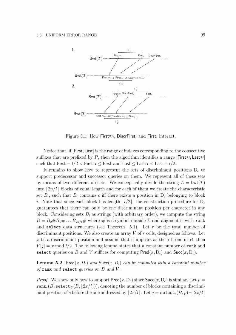
5.3. UNIFORM ERROR RANGE 99
First ≈iDiscrFirsti Firsti
Bwt(T )
Bwt(T )
≤ l
2
Firsti−1First ≈i−1
≤ l
2
LF(DiscrFirst ≈i−1)
First ≈i DiscrFirstiFirstiBwt(T )
Bwt(T )
≤ l
2
Firsti−1First ≈i−1
≤ l
2
LF(DiscrFirst ≈i−1)
1.
2.
Figure 5.1: How First≈i, DiscrFirsti and Firsti interact.
Notice that, if [First, Last] is the range of indexes corresponding to the consecutive
suffixes that are prefixed by P , then the algorithm identifies a range [First≈, Last≈]
such that First− l/2 < First≈ ≤ First and Last ≤ Last≈ < Last + l/2.
It remains to show how to represent the sets of discriminant positions Dc to
support predecessor and successor queries on them. We represent all of these sets
by means of two different objects. We conceptually divide the string L = bwt(T )
into d2n/le blocks of equal length and for each of them we create the characteristic
set Bi, such that Bi contains c iff there exists a position in Dc belonging to block
i. Note that since each block has length bl/2c, the construction procedure for Dc
guarantees that there can only be one discriminant position per character in any
block. Considering sets Bi as strings (with arbitrary order), we compute the string
B = B0#B1# . . . B2n/l# where # is a symbol outside Σ and augment it with rank
and select data structures (see Theorem 5.1). Let r be the total number of
discriminant positions. We also create an array V of r cells, designed as follows. Let
x be a discriminant position and assume that it appears as the jth one in B, then
V [j] = x mod l/2. The following lemma states that a constant number of rank and
select queries on B and V suffices for computing Pred(x,Dc) and Succ(x,Dc).
Lemma 5.2. Pred(x,Dc) and Succ(x,Dc) can be computed with a constant number
of rank and select queries on B and V .
Proof. We show only how to support Pred(x,Dc) since Succ(x,Dc) is similar. Let p =
rankc(B, select#(B, b2x/lc)), denoting the number of blocks containing a discrimi-
nant position of c before the one addressed by b2x/lc. Let q = selectc(B, p)−b2x/lc

100 CHAPTER 5. APPROXIMATE SUBSTRING SELECTIVITY ESTIMATION
be the index of the discriminant position preceding x (the subtraction removes the
# spurious symbols). Then, g = rank#(B, selectc(B, p)) finds the block preced-
ing (or including) b2x/lc that has a discriminant position for c. Also, V [q] con-
tains the offset, within that block, of the discriminant position. Such position can
be either in a block preceding b2x/lc or in the same block. In the former case,
Pred(x,Dc) = b2x/lcg + V [q]. In latter case we have an additional step to make,
as we have so far retrieved a position that just belongs to the same block of x but
could be greater than x. If that happens, we decrease p by 1 and repeat all the
calculations. Note that since the first occurrence of c is also a discriminant than
this procedure can never fail.
Once we have computed the correct discriminant positions, Algorithm 1 requires
to compute an LF-step from them (lines 7 and 9). The following Lemma states that
this task is simple.
Fact 5.1. For any symbol c, given any discriminant position d in Dc but the largest
one, we have that LF(d) = C[c]+(i−1) · l/2+1 where i is such that Dc’s ith element
in left-to-right position is d. For the largest discriminant position d in Dc we have
LF(d) = C[c+ 1].
It follows immediately that while performing the calculations of Lemma 5.2 we
can also compute the LF mapping of the discriminant position retrieved.
Proof of Theorem 5.2
Correctness has been proved. The time complexity is easily seen to be O(|P |)applications of Lemma 5.2, hence the claim. The space complexity is given by three
elements. The array C, containing counters for each symbol, requires O(σ log n)
bits. The number of discriminant positions is easily seen to be at most 2n/l in total,
hence the array V requires at most O(n/l) cells of O(log l) bits each. Finally, the
string B requires one symbol per block plus one symbol per discriminant position,
accounting for O(n log σ/l) bits in total. The theorem follows.
5.4 Lower-side error range
Let PST l(T ) be the pruned suffix tree as discussed in Section 5.1, and let m be the
number of its nodes. Recall that PST l(T ) is obtained from the suffix tree of T by
removing all the nodes with less than l leaves in their subtrees, and hence constitutes
a good solution to our lower-sided error problem: when Count(P ) ≥ l, the answer
is correct, otherwise an arbitrary number below l can be returned. Compared with

5.4. LOWER-SIDE ERROR RANGE 101
the solution of Section 5.3, it has the great advantage of being perfectly correct if
the pattern appears frequently enough, but it is extremely space inefficient. Our
objective in this section is to present a compact version of PST l(T ), by means of
proving the following theorem.
Theorem 5.4. Given T [1, n] drawn from an alphabet Σ of size σ and given an error
threshold l , there exists a representation of PST l(T ) using O(m log(σl) + σ log n)
bits that can answer to Count≥l(P ) in O(|P |×f(σ)) time where m is the number of
nodes of PST l(T ) and f(σ) is the chosen rank and select time complexity summed
up (see Theorem 5.1).
To appreciate Theorem 5.4, consider that the original PST l(T ) representation
requires, apart from node pointers, to store labels together with their lengths, for a
total of O(m log n+g log σ). The predominant space complexity is given by the edge
labels, since it can reach n log σ bits even when m is small. Therefore, our objective
is to build an alternative search algorithm that does not require all the labels to be
stored.
5.4.1 Computing counts
As a crucial part of our explanation, we will refer to nodes using their preorder traver-
sal times, with an extra requirement. Recall from Section 5.2.1 that the branching
symbol in a set of children of node u is the first symbol of children edge labels.
During the visit we are careful to descend into children in ascending lexicographical
order over their branching symbols. Therefore, u < v iff u is either an ancestor
of v or their corresponding path labels have the first mismatching symbols, say in
position k, such that pathlabel(u)[k] < pathlabel(v)[k].
We begin by explaining how to store and access the basic information that our
algorithm must recover: Given a node u ∈ PST l(T ) we would like to compute C(u),
the number of occurrences of pathlabel(u) as a substring in T 3. A straightforward
storage of such data would require m log n bits for a tree of m nodes. We prove
we can obtain better bounds and still compute C(u) in O(1) time, based on the
following simple observation:
Observation 5.1. Let u be a node in PST l(T ) and let v1, v2, . . . , vk be the children
of u in PST l(T ) that have been pruned away. Denote by g(u) the sum C(v1) +
C(v2) + · · ·+ C(vk). Then g(u) < σl .
Proof. Each of the vis represents a suffix that has been pruned away, hence, for any
i, it holds C(vi) < l by definition. Since each node can have at most σ children, the
observation follows.3Notice that C(u) is the number of leaves in the subtree of u in the original suffix tree.

102 CHAPTER 5. APPROXIMATE SUBSTRING SELECTIVITY ESTIMATION
Note that Observation 5.1 applies in a stronger form to leaves, where for a
leaf x, C(x) = g(x). We refer to the g(·) values as correction factors (albeit for
leaves they are actual counts). For an example refer to Figure 5.6. It is easy
to see that to obtain C(v) it suffices to sum all the correction factors of all the
descendants of v in PST l(T ). Precisely, it suffices to build the binary string G =
0g(0)10g(1)1 · · ·0g(m−1)1 together with support for binary select queries.
Lemma 5.3. Let v ∈ PST l(T ) and let z be the identifier of its rightmost leaf. Define
CNT(u, z) = select1(G, z)− z − select1(G, u) + u. Then C(u) = CNT(u, z).
Proof. By our numbering scheme, [u, z] contains all values in G for nodes in the
subtree of u. select1(G, x)−x is equivalent to rank0(G, select1(G, x)), i.e. it sums
up all correction factors in nodes before x in the numbering scheme. Computing the
two prefix sums and subtracting is sufficient.
Lemma 5.4. Let m be the number of nodes in PST l(T ), then G can be stored using
at most m log(σl) +O(m) bits and each call CNT(u, z) requires O(1) time.
Proof. Each correction factor has size σl at most, hence the number of 0s in G is at
most mσl . The number of 1s in G is m. The thesis follows by storing G with the
binary Elias-Fano data structure of Section 2.5.1.
5.4.2 Finding the correct node
When explaining our solution, we will resort to the concepts of suffix links and
inverse suffix links in a suffix tree. For each node u of PST l(T ), the suffix link
SL(u) is v iff we obtain pathlabel(v) from pathlabel(u) by removing the first letter of
the string represented by u. The inverse suffix link (also referred to as Weiner link)
of v for some symbol c, denoted ISL(v, c), is u iff u = SL(v) and the link symbol is
c. We say that v possesses an inverse suffix link for c if ISL(v, c) is defined. We also
refer to the lowest common ancestor of two nodes u and v as LCA(u, v). An inverse
suffix link ISL(u, c) = v exists only if pathlabel(v) = c · pathlabel(u), however many
search algorithms require also virtual inverse suffix links to be available. We say a
node w has a virtual inverse suffix link for symbol c (denoted VISL(w, c)) if and only
if at least one of its descendants (including w) has an inverse suffix link for c. The
value of VISL(w, c) is equal to ISL(u, c) where u is the highest descendant of w having
an inverse suffix link for c4. As we will see in Lemma 5.7, it is guaranteed that this
highest descendant is unique and, thus, this definition is always well formed. The
intuitive meaning of virtual suffix links is the following: VISL(w, c) links node w to
the highest node w′ in the tree whose path label is prefixed by c · pathlabel(w).
4Notice that w and u are the same node whenever w has an inverse suffix link for c.

5.4. LOWER-SIDE ERROR RANGE 103
Our interest in virtual inverse suffix links is motivated by an alternative inter-
pretation of the classic backward search. When the backward search is performed,
the algorithm virtually starts at the root of the suffix tree, and then traverses (vir-
tual) inverse suffix links using the pattern to induce the link symbols, prefixing a
symbol at the time to the suffix found so far. The use of virtual inverse suffix links
is necessary to accommodate situations in which the pattern P exists but only an
extension P · α of it appears as a node in the suffix tree. Note that the algorithm
can run directly on the suffix tree if one has access to virtual inverse suffix links, and
such property can be directly extended to pruned suffix trees. Storing virtual inverse
suffix links explicitly is prohibitive since there can be up to σ of them outgoing from
a single node, therefore we plan to store real inverse suffix links and provide a fast
search procedure to evaluate the VISL function.
In the remaining part of this section we will show a few properties of (virtual)
suffix links that allow us to store/access them efficiently and to derive a proof of
correctness of the search algorithm sketched above.
The following two lemmas 5 state that inverse suffix links preserve the relative
order between nodes.
Lemma 5.5. Let w, z be nodes in PST l(T ) such that ISL(w, c) = w′ and ISL(z, c) =
z′. Let u = LCA(w, z) and u′ = LCA(w′, z′). Then, ISL(u, c) = u′.
Proof. If w is a descendant of z or viceversa, the lemma is proved. Hence, we assume
u 6= w and u 6= z. Let α = pathlabel(u). Since u is a common ancestor of w and z,
it holds pathlabel(w) = α · β and pathlabel(z) = α · ζ for some non-empty strings β
and ζ. By definition of inverse suffix link, we have that pathlabel(w′) = c · α · β and
pathlabel(z) = c · α · ζ. Since w and z do not share the same path below u, the first
symbols of β and ζ must differ. This implies the existence of a node v whose path
label is pathlabel(v) = c ·α which is the lowest common ancestor between w′ and z′.
Again by definition of inverse suffix link, it follows that ISL(u, c) = u′ = v.
Lemma 5.6. Given any pair of nodes u and v with u < v such that both have an
inverse suffix link for symbol c, it holds ISL(u, c) < ISL(v, c).
Proof. Since u < v, we have that pathlabel(u) is lexicographically smaller than
pathlabel(v). Thus, obviously c · pathlabel(u) is lexicographically smaller than c ·pathlabel(v). Since c·pathlabel(u) is the path label of u′ = ISL(u, c) and c·pathlabel(v)
is the path label of v′ = ISL(v, c), u′ precedes v′ in the preorder traversal of PST l(T ).
5The same property of Lemma 5.5 is also observed in [RNO11] (Lemma 5.1).

104 CHAPTER 5. APPROXIMATE SUBSTRING SELECTIVITY ESTIMATION
Computing the virtual inverse suffix link of node u for symbol c requires to
identify the highest descendant of u (including u) having an inverse suffix link for
c. If such a node does not exist we conclude that the virtual inverse suffix link
is undefined. The following lemma states that such node, say v, must be unique
meaning that if there exists an other descendant of u having an inverse suffix link
for c, then this node must also be a descendant of v.
Lemma 5.7. For any node u in PST l(T ), the highest descendant of u (including
u) having an inverse suffix link for a symbol c, if existing, is unique.
Proof. Pick any pair of nodes that descend from u having an inverse suffix link for
the symbol c. By Lemma 5.5 their common ancestor must also have an inverse suffix
link for c. Thus, there must exist a unique node that is a common ancestor of all of
these nodes.
In our solution we conceptually associate each node u in PST l(T ) with the
set of symbols Du for which u has an inverse suffix link. We represent each set
with a string Enc(Du) built by concatenating the symbols in Du in any order
and ending with a special symbol # not in Σ. We then build a string S as
Enc(D0)Enc(D1) · · ·Enc(Dm−1) so that the encodings follow the preorder traver-
sal of the tree 6. We also define the array C[1, σ] whose entry C[c] stores the
number of nodes of PST l(T ) whose path label starts with a symbol lexicographi-
cally smaller than c. The next theorem proves that string S together with rank and
select capabilities is sufficient to compute VISL. This is crucial to prove that our
data structure works, proving virtual inverse suffix links can be recreated from real
ones.
Theorem 5.5. Let u ∈ PST l(T ) and let z be the rightmost leaf descending from
u. For any character c ∈ Σ, let cu = rankc(S, select#(S, u − 1)) and, similarly,
let cz = rankc(S, select#(S, z)). Then (a) if cu = cz, VISL(u, c) is undefined.
Otherwise, (b) VISL(u, c) = C[c] + cu + 1 and (c) C[c] + cz is the rightmost leaf
descending from VISL(u, c).
Proof. Let A be the set of nodes of PST l(T ) whose path label is lexicographically
smaller than the path label of u and let B be the set of nodes in the subtree of
u. Let S(A) and S(B) be the concatenations of, respectively, Enc(Dw) for w ∈ Aand Enc(Dw) for w ∈ B. Due to the preorder numbering of nodes, we know that
A = [0, u−1] and B = [u, z]. Thus, S(A) is a prefix of S that ends where S(B) begins.
Notice that the operations select#(S, u−1) and select#(S, z) return respectively
6Interestingly, a similar method of traversing a suffix tree by means of inverse suffix links
encoded in a string has been proposed in [ANS12]

5.4. LOWER-SIDE ERROR RANGE 105
Algorithm Count≥l (P [1, p])
1. i = p, c = P [p], up = C[c] + 1, zp = C[c+ 1];
2. while ((ui 6= zi) and (i ≥ 2)) do
3. c = P [i− 1];
4. ui−1 = VISL(ui, c) = C[c] + rankc(S, select#(S, ui)) + 1;
5. zi−1 = VISL(zi, c) = C[c] + rankc(S, select#(S, zi));
6. i = i− 1;
7. if (ui = zi) then return “no occurrences of P” else return CNT(u1, z1)
Figure 5.2: Our algorithm to report the number of occurrences of a pattern P [1, p]
in our Compact Pruned Suffix Tree.
the ending positions of S(A) and S(B) in S. Thus, cu counts the number of inverse
suffix links of nodes in A while cz includes also the number of inverse suffix links
of nodes in B. Hence, if cu = cz no node of B has an inverse suffix link and, thus,
proposition (a) is proved.
By Lemma 5.6 we know that inverse suffix links map nodes preserving their
relative order. Thus, the first node in B that has an inverse suffix link for c is
mapped to node C[c] + cu + 1.7 By the node numbering, this first node is obviously
also the highest one. Thus, proposition (b) is proved.
Proposition (c) is proved by resorting to similar considerations.
Figure 5.7 illustrates the whole situation. Exploiting VISL, Algorithm 5.2 searches
for a pattern P [1, p] backwards. The algorithm starts by setting up to be C[P [p]]+1.
At the ith step, we inductively assume that ui+1 is known, and that its path label
is prefixed by P [i + 1, p]. Similarly, we keep zi+1, the address of the rightmost leaf
in u’s subtree. Using ui+1 and zi+1 we can evaluate if VISL(ui+1, P [i]) and, in such
case, follow it. In the end, we have to access the number of suffixes of T descending
from u1. The next theorem formally proves the whole algorithm correctness:
Theorem 5.6. Given any pattern P [1, p], Algorithm 5.2 retrieves C(u), where u is
the highest node of PST l(T ) such that pathlabel(u) is prefixed by P . If such node
does not exist, it terminates reporting −1.
7There is a caveat: in case the first node of the subtree of c has an edge label with length greater
than 1, then the +1 factor must be eliminated, since that same node becomes a destination.

106 CHAPTER 5. APPROXIMATE SUBSTRING SELECTIVITY ESTIMATION
Proof. We start by proving that such node u, if any, is found, by induction. It is
easy to observe that C[P [p]] + 1 is the highest node whose path label is prefixed by
the single symbol P [p].
By hypothesis, we assume that ui+1 is the highest node in PST l(T ) whose
path label is prefixed by P [i + 1, p], and we want to prove the same for ui =
VISL(ui+1, P [p − i]). The fact that pathlabel(ui) is prefixed by P [p − i, p] easily
follows by definition of inverse suffix link. We want to prove that ui is the highest
one with this characteristic: by contradiction assume there exists another node w′
higher that ui = VISL(ui+1, P [i]). This implies that there exists a node w = SL(w′),
prefixed by P [i+ 1, p]. Also, the virtual inverse suffix link of ui+1 is associated with
a proper one whose starting node is z = SL(ui+1), which by definition of VISL is also
the highest one in u’s subtree. Thus, by Lemma 5.7, w is a descendant of z. Hence,
w > z but ISL(w′, c) < ISL(z, c), contradicting Lemma 5.6.
Finally, if at some point of the procedure a node ui+1 does not have a virtual
inverse suffix link, then it is straightforward that the claimed node u does not exist
(i.e. P occurs in T less than l times). Once u is found, also z is present, hence we
resort to Lemma 5.3 to obtain C(u) = CNT(u, z).
Proof of Theorem 5.4
We need to store: the C array, holding the count of nodes in PST l(T ) whose
path label prefixed by each of the σ characters; the string G, together with binary
select capabilities and the string S, together with arbitrary alphabet rank and
select capabilities. Let m be the number of nodes in PST l(T ). We know C
occupies at most σ log n bits. By Lemma 5.4 G occupies at most m log(σl) +O(m)
bits. String S can be represented in different ways, related to σ, picking a choice
from Theorem 5.1, but the space is always limited by m log σ + o(m log σ). Hence
the total space is σ log n+m log(σl)+O(m)+O(m log(σ)) = O(m log(σl)+σ log n),
as claimed. For the time complexity, at each of the p steps, we perform four rank
and select queries on arbitrary alphabets which we account as f(σ). The final step
on G takes O(1) time, hence the bound.
5.5 Lower bounds
The following lower bound proves the minimum amount of space needed to solve
the substring occurrence estimation problem for both error ranges, uniform and
lower-sided.

5.6. EXPERIMENTS 107
Theorem 5.7. For a fixed additive error l ≥ 1, an index built on a text T [1, n]
drawn from an alphabet Σ of size σ that approximates the number of occurrences of
any pattern P in T within l must use Ω(n log(σ)/l) bits of space.
Proof. Assume there exists an index requiring o(n log(σ)/l) bits of space and an-
swering any approximate counting query within an additive error l . Given any text
T [1, n], we derive a new text T ′[1, (l + 1)(n + 1)] that is formed by repeating the
string T# for l + 1 times, where $ is a symbol that does not belong to Σ. Then,
we build the index on T ′ that requires o((l + 1)(n + 1) log(σ + 1)/l) = o(n log σ)
bits. We observe that we can recover the original text T by means of this index:
we search all possible strings of length n drawn from Σ followed by a #, the only
one for which the index answers with a value greater than l is T . A random (in
Kolmogorov’s sense) text has entropy log(σn)−O(1) = n log σ −O(1) bits. Hence,
the index would represent a random text using too few bits, a contradiction.
Using the same argument we can prove the following Theorem, which justifies
the need of focusing on additive errors.
Theorem 5.8. For a fixed multiplicative error (1 + ε) > 1, an index built on a
text T [1, n] drawn from an alphabet Σ of size σ that approximates the number of
occurrences of any pattern P in T within (1 + ε) must use Ω(n log σ) bits of space.
5.6 Experiments
In this section we show an experimental comparison among the known solutions
and our solutions. We use four different data sets downloaded from Pizza&Chili
corpus [FGNV08] that correspond to four different types of texts: DNA sequences,
structured text (XML), natural language and source codes. Text and alphabet size
for the texts in the collection are reported in the first column of Table 5.1.
We compare the following solutions:
• FM-index (v2). This is an implementation of a compressed full-text index
available at the Pizza&Chili site [FGNV08]. Since it is the compressed full-
text index that achieves the best compression ratio, it is useful to establish
which is the minimum space required by known solutions to answer to counting
queries without errors.
• APPROX-l . This is the implementation of our solution presented in Section 5.3.
• PST-l . This is an implementation of the Pruned Suffix Tree as described in
[KVI96].

108 CHAPTER 5. APPROXIMATE SUBSTRING SELECTIVITY ESTIMATION
Data set Size Alphabet size ( σ )
dblp 275 96
dna 292 15
english 501 225
sources 194 229
Setl = 8 l = 64 l = 256
|T |/l |PST l |∑ |edgei| |T |/l |PST l |
∑ |edgei| |T |/l |PST l |∑ |edgei|
dblp 36064 28017 1034K 4508 3705 103K 1127 941 20K
dna 38399 42361 815K 4799 5491 102K 1199 1317 19K
english 65764 53600 661K 8220 6491 64K 2055 1616 14K
sources 25475 25474 11376K 3184 3264 9430K 796 982 8703K
Table 5.1: Statistics on the data sets. The second column denotes the original
text in MBytes. Each group of three columns in the lower table describe PST l
information for a choice of `: expected amount of nodes, |T |/l ; real amount of nodes
in PST l(T ); sum of length of labels in PST l(T ).
• CPST-l . This is the implementation of our Compact Pruned Suffix Tree de-
scribed in Section 5.4.
Recall that APPROX-l reports results affected by an error of at most l while PST-l
and CPST-l are always correct whenever the pattern occurs at least l times in the
indexed text.
The plots in Figure 5.3 show the space occupancies of the four indexes depending
on the chosen threshold l . We do not plot space occupancies worse than FM-index,
since in those cases FM-index is clearly the index to choose. In fact, Figure 5.3(d)
does not contain a plot for PST, since its space performance was always worse thanFM-index.
It turns out that in all the texts of our collection the number of nodes in the
pruned suffix tree is small (even smaller than n/l): these statistics are reported in
Table 5.1. This is the reason why our CPST is slightly more space-efficient than
APPROX. In practice, the former should be indubitably preferred with respect to the
latter: it requires less space and it is always correct for patterns that occur at least
l times. Even though, the latter remains interesting due to its better theoretical
guarantees. In both solutions, by halving the error threshold, we obtain indexes
that are between 1.75 (CPST) and 1.95 (APPROX) times smaller. Thus, we can obtain
very small indexes by setting relatively small values of l . As an example, CPST with
l = 256 on text english requires 5.1 Mbytes of space which is roughly 100 times
smaller than the original text. We observe that both CPST and APPROX are in general
significantly smaller than FM-index and remain competitive even for small values of

5.6. EXPERIMENTS 109
0
10
20
30
40
50
60
70
8 16 32 64 128 256
Spa
ce (
Mby
tes)
Error Threshold
(a) dblp
0
20
40
60
80
100
120
8 16 32 64 128 256
Spa
ce (
Mby
tes)
Error Threshold
(b) dna
0
50
100
150
200
250
8 16 32 64 128 256
Spa
ce (
Mby
tes)
Error Threshold
(c) english
0
10
20
30
40
50
60
70
80
90
8 16 32 64 128 256
Spa
ce (
Mby
tes)
Error Threshold
(d) sources
• FM-index APPROX × PST CPST
Figure 5.3: Space occupancies of indexes as a function of the error threshold l .
l . As an example, FM-index requires 232.5 Mbytes on english ,which is roughly 45
times larger than CPST−256.
As far as PST is concerned, it is always much worse than CPST and APPROX. As
expected, its space inefficiencies are due to the need of storing edge labels since their
amount grows rapidly as l decreases (see Table 5.1). Moreover, this quantity strictly
depends on the indexed text, while the number of nodes is more stable. Thus, the
performances of PST are erratic: worse than CPST by a factor 6 on english that
becomes 60 on sources. It is remarkable that on sources we have to increase PST’s
error threshold up to 11, 000 to achieve a space occupancy close to our CPST with
l = 8 .
For what concerns applications, we use our best index, i.e. CPST together with
one estimation algorithm: MOL. The reader can find a brief explanation of the algo-
rithm in Section 5.2.4; the algorithm is oblivious to the underlying data structure as
long as a lower-sided error one is used. We performed (details omitted) a compari-
son between MO, MOL and KVI [KVI96, JNS99] and found out that MOL delivered the
best estimates. We also considered MOC and MOLC, but for some of our data sets the
creation of the constraint network was prohibitive in terms of memory. Finally, we
tried to compare with CRT [CGG04]; however, we lacked the original implementation

110 CHAPTER 5. APPROXIMATE SUBSTRING SELECTIVITY ESTIMATION
Data set Indices |P | = 6 |P | = 8
dblpPST-256 10.06 ± 32.372 12.43 ± 34.172
CPST-16 0.68 ± 1.456 0.86 ± 1.714
dnaPST-256 0.47 ± 1.048 0.49 ± 2.433
CPST-32 0.47 ± 0.499 0.43 ± 0.497
englishPST-256 7.03 ± 27.757 12.45 ± 31.712
CPST-32 0.80 ± 2.391 1.40 ± 3.394
sourcesPST-11000 816.06 ± 1646.57 564.94 ± 1418.53
CPST-8 0.70 ± 1.028 0.93 ± 1.255
Data set Indices |P | = 10 |P | = 12 Average Improvement
dblpPST-256 14.20 ± 35.210 15.57 ± 36.044
CPST-16 1.00 ± 1.884 1.14 ± 2.00919.03×
dnaPST-256 4.26 ± 15.732 11.09 ± 19.835
CPST-32 0.52 ± 0.904 1.77 ± 2.9765.51×
englishPST-256 13.81 ± 28.897 11.43 ± 23.630
CPST-32 2.07 ± 3.803 2.45 ± 3.6239.68×
sourcesPST-11000 400.62 ± 1229.35 313.68 ± 1120.94
CPST-8 1.13 ± 1.367 1.28 ± 1.394792.52×
Figure 5.4: Comparison of error (difference between number of occurrences and
estimate) for MOL estimates over different pattern lengths. PST and CPST parameters
are chosen to obtain close index sizes. Tests performed on 1M random patterns
appearing in the text. The last column shows the average factor of improvement
obtained by using our CPST instead of PST.
and a significative training set for our data sets. Hence, we discarded the algorithm
from our comparison.
Figure 5.4 shows the average error of the estimates obtained with MOL on our
collection by using either CPST or PST as the base data structure. For each set
we identified two pairs of thresholds such that our CPST and PST have roughly
the same space occupancy. For each text, we searched for 4 million patterns of
different lengths that we randomly extracted from the text. Thus, this figure depicts
the significant boost in accuracy that one can achieve by replacing PST with our
solution. As an example, consider the case of sources where the threshold of PST
is considerably high due to its uncontrollable space occupancy. In this case the
factor of improvement that derives by using our solution is more than 790. The
improvements for the other texts are less impressive but still considerable.
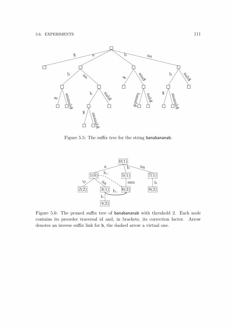
5.6. EXPERIMENTS 111
$ anan
ab$
b nab$
ban
ab$
nab
$
$
ana$
$ anan
ab$
b nab$$
anan
ab$
b na
$ a b na
Figure 5.5: The suffix tree for the string banabananab.
0(1)
7(1)
8(2)
b
5(1)
6(2)
ana
1(0)
3(1)
4(2)
b
2(2)
b na
a b na
b..
b..
Figure 5.6: The pruned suffix tree of banabananab with threshold 2. Each node
contains its preorder traversal id and, in brackets, its correction factor. Arrow
denotes an inverse suffix link for b, the dashed arrow a virtual one.

112 CHAPTER 5. APPROXIMATE SUBSTRING SELECTIVITY ESTIMATION
a,b,n
a
ab
aana
b,n
bb
n
b na
a b na
S =ab#n#n#b##a##a#a#
Figure 5.7: The same PST of Figure 5.6, with information associated with Theorem
5.5. Each node is given the set of symbols for which a virtual inverse suffix link
is defined. The string S contains the separated encoding, in preorder traversal, of
suffix links chosen by our procedure. Note that the first child with edge label a loses
its link for b, as ana is sufficient.

Chapter 6
Future directions
We conclude the thesis by presenting various missing results, hoping to inspire fur-
ther research on the matter.
Binary, distribution aware rank and select.
The work on predecessor search and binary rank/select has been very thorough
and in the late years brought up amazing results in terms of upper and lower bound.
The basic line of research, i.e. just considering u, n and t to create data structures, is
almost fulfilled. Nevertheless, real data is usually correlated to specific distributions
(e.g. gap lists for indexing). In massive data sets analysis skewed mixtures of bino-
mials or power law distributions are very frequent [WMB99]. Sometimes, through
permutations over the universe, bitvectors can be made clustered (see e.g. [BB02])
so that 1s concentrate in contiguous regions. rank and select data structures that
take into account such parameters are not known yet. Practical work [Vig08] al-
ready proved that different density (u/n) factors can help choosing the correct data
structure. It would be interesting to understand how much powerful a data struc-
ture can become if the generating source is well known. We conjecture that sensible
lowering in total space may be achieved.
select and contiguous memory access.
The index built for select over strings in Theorem 4.6 is an application of the code
for permutation inversions presented in [MRRR03]. The original definition regards
a permutation π over [n] that has to be inverted, and produces an index where one
follows the cycles of π starting from some position x until one finds y such that
π(y) = x, i.e. π−1(x). To limit the number of evaluation of π they insert shortcuts
in the permutation cycles every t jumps, for some t. The original index is optimal
when w = Θ(log n). In the Word RAM model, however, we may have w = ω(log n).

114 CHAPTER 6. FUTURE DIRECTIONS
In theory this should bring the redundancy of the data structure down accordingly,
also considering situations in which more elements of the permutation can be stored
in one word. So far, no progress has been done on the front and no lower bounds
have been proposed. Having either a lower or upper bound would have a significant
impact: the BWT LF mapping that one has to follow in the classic BWT inversion
procedure is exactly equivalent to following a permutation; a better upper bound
would probably give an advantage at decompressing when the alphabet is small; a
lower bound would finally justify a limit to research in that sense. In our setting, this
would prove that a better select for indexes in the Word RAM model is possible.
Practical constant-alphabet rank and select.
The case of σ = 2 has been studied in practice (see e.g. [GGMN05, OS07, Vig08]),
as well as the generic case of any σ (see e.g. [CN08]). However, the two kinds of
solutions are completely apart, e.g. the latter involves quite complex and impractical
machinery and cannot easily compete with the speed of binary solutions. It is
still the case that constant time alphabets may need to be used, i.e. σ = 3 or 4
(an example is BWT over DNA). Adapting binary solutions to this scenario is not
stragithforward if one wants to keep space consumption low. We think it is worth
investigating on that front, producing data structures that can perform rank and
select in competitive times for relatively small alphabets.
Small and fast construction of CPST l .
The CPST l of Section 5.4 can be constructed with an easy algorithm. Namely, one
can build the full suffix tree and then prune it. This is slow and, worse, extremely
memory consuming: a suffix tree can have O(n) nodes for a string of length n; when `
is small this is extremely wasteful. We call for a more efficient and fast construction
algorithm in theory at first. Given the final space consumption we also consider
important to perform research of a practically employable construction algorithm.

Bibliography
[Ajt88] Miklos Ajtai. A lower bound for finding predecessors in yao’s call probe
model. Combinatorica, 8(3):235–247, 1988.
[ANS12] Diego Arroyuelo, Gonzalo Navarro, and Kunihiko Sadakane. Stronger
lempel-ziv based compressed text indexing. Algorithmica, 62(1):54–
101, 2012.
[BB02] Dan Blandford and Guy Blelloch. Index compression through docu-
ment reordering. In Proceedings of the Data Compression Conference,
DCC ’02, pages 342–, 2002.
[BB04] Daniel K. Blandford and Guy E. Blelloch. Compact representations
of ordered sets. In Proceedings of the fifteenth annual ACM-SIAM
symposium on Discrete algorithms, SODA ’04, pages 11–19, 2004.
[BBPV09] Djamal Belazzougui, Paolo Boldi, Rasmus Pagh, and Sebastiano Vigna.
Monotone minimal perfect hashing: searching a sorted table with O(1)
accesses. In Proc. of the 20th ACM-SIAM SODA, pages 785–794, 2009.
[BBPV10] D. Belazzougui, P. Boldi, R. Pagh, and S. Vigna. Fast prefix search in
little space, with applications. In ESA (1), pages 427–438, 2010.
[BCN10] Jeremy Barbay, Francisco Claude, and Gonzalo Navarro. Compact rich-
functional binary relation representations. In LATIN, pages 170–183,
2010.
[BDM+05] David Benoit, Erik D. Demaine, J. Ian Munro, Rajeev Raman,
Venkatesh Raman, and S. Srinivasa Rao. Representing trees of higher
degree. Algorithmica, 43(4):275–292, 2005.
[BF02] P. Beame and F.E. Fich. Optimal bounds for the predecessor problem
and related problems. J. Comput. Syst. Sci, 65:38–72, 2002.

116 CHAPTER 6. BIBLIOGRAPHY
[BGNN10] J. Barbay, T. Gagie, G. Navarro, and Y. Nekrich. Alphabet partitioning
for compressed rank/select and applications. In ISAAC (2), pages 315–
326, 2010.
[BHMR07a] J. Barbay, M. He, J.I. Munro, and S. Srinivasa Rao. Succinct in-
dexes for string, binary relations and multi-labeled trees. In Proc.
ACM-SIAM Symposium on Discrete Algorithms (SODA), pages 680–
689, 2007.
[BHMR07b] Jeremy Barbay, Meng He, J. Ian Munro, and S. Srinivasa Rao. Succinct
indexes for strings, binary relations and multi-labeled trees. In Proc.
of the 18th ACM-SIAM SODA., pages 680–689, 2007.
[BHMR07c] Jeremy Barbay, Meng He, J. Ian Munro, and S. Srinivasa Rao. Suc-
cinct indexes for strings, binary relations and multi-labeled trees – full
version, 2007.
[BM99] A. Brodnik and J.I. Munro. Membership in constant time and almost-
minimum space. SIAM J. Computing, 28:1627–1640, 1999.
[BN11a] Djamal Belazzougui and Gonzalo Navarro. New lower and upper
bounds for representing sequences. In ESA, 2011.
[BN11b] Djamal Belazzougui and Gonzalo Navarro. New lower and upper
bounds for representing sequences. CoRR, abs/1111.2621, 2011.
[BPZ07] Fabiano C. Botelho, Rasmus Pagh, and Nivio Ziviani. Simple and
space-efficient minimal perfect hash functions. In In Proc. of the 10th
Intl. Workshop on Data Structures and Algorithms, pages 139–150.
Springer LNCS, 2007.
[BW94] M. Burrows and D. Wheeler. A block sorting lossless data compres-
sion algorithm. Technical Report 124, Digital Equipment Corporation,
1994.
[BYRN11] Ricardo Baeza-Yates and Balazs Ribeiro-Neto. Modern Information
Retrieval (2nd edition). ACM Press Book, 2011.
[CGG04] S. Chaudhuri, V. Ganti, and L. Gravano. Selectivity estimation for
string predicates: Overcoming the underestimation problem. In Pro-
ceedings of the 20th International Conference on Data Engineering,
ICDE ’04, pages 227–, 2004.

6.0. BIBLIOGRAPHY 117
[CKL+06] Cheng T. Chu, Sang K. Kim, Yi A. Lin, Yuanyuan Yu, Gary R. Brad-
ski, Andrew Y. Ng, and Kunle Olukotun. Map-Reduce for Machine
Learning on Multicore. In Bernhard Scholkopf, John C. Platt, and
Thomas Hoffman, editors, NIPS, pages 281–288. MIT Press, 2006.
[Cla96] D. Clark. Compact Pat Trees. PhD thesis, University of Waterloo,
1996.
[CLRS00] T. H. Cormen, C. E. Leiserson, R. L. Rivest, and C. Stein. Introduction
to Algorithms, 2nd edition. MIT Press, McGraw-Hill Book Company,
2000.
[CN08] F. Claude and G. Navarro. Practical rank/select queries over arbitrary
sequences. In Proc. 15th (SPIRE), LNCS. Springer, 2008.
[CT06] T. M. Cover and J. A. Thomas. Elements of Information Theory
(Wiley Series in Telecommunications and Signal Processing). Wiley-
Interscience, 2006.
[DBCP97] Mikael Degermark, Andrej Brodnik, Svante Carlsson, and Stephen
Pink. Small forwarding tables for fast routing lookups. In SIGCOMM,
pages 3–14, 1997.
[DG08] Jeffrey Dean and Sanjay Ghemawat. Mapreduce: simplified data pro-
cessing on large clusters. Commun. ACM, 51:107–113, January 2008.
[DLO03] Erik D. Demaine and Alejandro Lopez-Ortiz. A linear lower bound on
index size for text retrieval. J. Algorithms, 48(1):2–15, 2003.
[Eli74a] P. Elias. Efficient storage and retrieval by content and address of static
files. J. Assoc. Comput. Mach., 21(2):246–260, 1974.
[Eli74b] Peter Elias. Efficient storage and retrieval by content and address of
static files. J. Assoc. Comput. Mach., 21(2):246–260, 1974.
[Fan71a] R. M. Fano. On the number of bits required to implement an associative
memory. Memorandum 61, Computer Structures Group, Project MAC,
1971.
[Fan71b] Robert M. Fano. On the number of bits required to implement an
associative memory. Memorandum 61, Computer Structures Group,
Project MAC, MIT, Cambridge, Mass., n.d., 1971.

118 CHAPTER 6. BIBLIOGRAPHY
[FG99a] P. Ferragina and R. Grossi. The string b-tree: a new data structure
for string search in external memory and its applications. J. ACM,
46:236–280, March 1999.
[FG99b] P. Ferragina and Roberto Grossi. The string b-tree: A new data struc-
ture for string search in external memory and its applications. J. of
the ACM, 46(2):236–280, 1999.
[FGNV08] P. Ferragina, R. Gonzalez, G. Navarro, and R. Venturini. Compressed
text indexes: From theory to practice. ACM Journal of Experimental
Algorithmics, 13, 2008.
[Fis10] Johannes Fischer. Optimal succinctness for range minimum queries. In
Alejandro Lpez-Ortiz, editor, LATIN 2010: Theoretical Informatics,
volume 6034 of Lecture Notes in Computer Science, pages 158–169.
Springer Berlin / Heidelberg, 2010.
[FM05] P. Ferragina and G. Manzini. Indexing compressed text. Journal of
the ACM, 52(4):552–581, 2005.
[FM08a] Arash Farzan and J. Munro. A uniform approach towards succinct
representation of trees. In Joachim Gudmundsson, editor, Algorithm
Theory SWAT 2008, volume 5124 of Lecture Notes in Computer Sci-
ence, pages 173–184. Springer Berlin / Heidelberg, 2008.
[FM08b] Arash Farzan and J. Ian Munro. Succinct representations of arbitrary
graphs. In Proceedings of the 16th annual European symposium on
Algorithms, ESA ’08, pages 393–404, 2008.
[FMMN04] Paolo Ferragina, Giovanni Manzini, Veli Makinen, and Gonzalo
Navarro. An alphabet-friendly fm-index. In SPIRE, pages 150–160,
2004.
[FMMN07] P. Ferragina, G. Manzini, V. Makinen, and G. Navarro. Compressed
representations of sequences and full-text indexes. ACM Transactions
on Algorithms, 3(2), 2007.
[FRR09] Arash Farzan, Rajeev Raman, and S. Srinivasa Rao. Universal succinct
representations of trees? In Proceedings of the 36th International Col-
loquium on Automata, Languages and Programming: Part I, ICALP
’09, pages 451–462, Berlin, Heidelberg, 2009. Springer-Verlag.

6.0. BIBLIOGRAPHY 119
[FV07] Paolo Ferragina and Rossano Venturini. A simple storage scheme for
strings achieving entropy bounds. Theor. Comput. Sci., 372(1):115–
121, 2007.
[FW94] M. Fredman and D. Willard. Surpassing the information theoretic
bound with fusion trees. J. Comput. System Sci.,, 47(3):424–436, 1994.
[GGG+07] A. Golynski, R. Grossi, A. Gupta, R. Raman, and S. S. Rao. On the
size of succinct indices. In Proc 15th ESA, LNCS 4698, pages 371–382,
2007.
[GGMN05] R. Gonzalez, Sz. Grabowski, V. Makinen, and G. Navarro. Practical
implementation of rank and select queries. In Proc. 4th (WEA), pages
27–38, 2005.
[GGV04] R. Grossi, A. Gupta, and J. S. Vitter. When indexing equals compres-
sion: experiments with compressing suffix arrays and applications. In
Proc. 15th ACM-SIAM SODA, pages 636–645, 2004.
[GHSV06] Ankur Gupta, Wing-Kai Hon, Rahul Shah, and Jeffrey Scott Vitter.
Compressed data structures: dictionaries and data-aware measures.
In In Proc. 5th International Workshop on Experimental Algorithms
(WEA), pages 158–169, 2006.
[GHSV07] A. Gupta, W. Hon, R. Shah, and Jeffrey Scott Vitter. Compressed data
structures: Dictionaries and data-aware measures. Theor. Comput. Sci,
387(3):313–331, 2007.
[GKP94] Ronald L. Graham, Donald E. Knuth, and Oren Patashnik. Concrete
Mathematics: A Foundation for Computer Science. Addison-Wesley
Longman Publishing Co., Inc., Boston, MA, USA, 2nd edition, 1994.
[GM07] A. Gal and P. Bro Miltersen. The cell probe complexity of succinct
data structures. Theor. Comput. Sci., 379:405–417, 2007.
[GMR06] Alexander Golynski, J. Ian Munro, and S. Srinivasa Rao. Rank/select
operations on large alphabets: a tool for text indexing. In Proc. of the
17th ACM-SIAM SODA, pages 368–373, 2006.
[GN06] Rodrigo Gonzalez and Gonzalo Navarro. Statistical encoding of suc-
cinct data structures. In Proc. 17th CPM, Lecture Notes in Computer
Science, pages 294–305. Springer, 2006.

120 CHAPTER 6. BIBLIOGRAPHY
[Gol07a] A. Golynski. Optimal lower bounds for rank and select indexes. Theor.
Comput. Sci., 387:348–359, 2007.
[Gol07b] A. Golynski. Upper and Lower Bounds for Text Indexing Data Struc-
tures. PhD thesis, University of Waterloo, 2007.
[Gol09] A. Golynski. Cell probe lower bounds for succinct data structures. In
Proc. of the 20th ACM-SIAM SODA, pages 625–632, 2009.
[GOR10] Roberto Grossi, Alessio Orlandi, and Rajeev Raman. Optimal trade-
offs for succinct string indexes. In Proc. of the 37th International Collo-
quim on Automata, Languages and Programming (ICALP), pages 678–
689, 2010.
[GORR09] Roberto Grossi, Alessio Orlandi, Rajeev Raman, and S. Srinivasa Rao.
More haste, less waste: Lowering the redundancy in fully indexable
dictionaries. In Proc. 26th STACS, pages 517–528, 2009.
[GORR11] Alexander Golynski, Alessio Orlandi, Rajeev Raman, and S. Srinivasa
Rao. Optimal indexes for sparse bit vectors. CoRR, abs/1108.2157,
2011.
[GORR12] Alexander Golynski, Alessio Orlandi, Rajeev Raman, and S. Srinivasa
Rao. Optimal indexes for sparse bit vectors. Algorithmica, In press.,
2012.
[GRR08] A. Golynski, R. Raman, and S. S. Rao. On the redundancy of succinct
indices. In Proc. 11th SWAT, pages 148–159, 2008.
[Gus97] D. Gusfield. Algorithms on Strings, Trees, and Sequences: Computer
Science and Computational Biology. Cambridge University Press, 1997.
[GV05] R. Grossi and J. S. Vitter. Compressed suffix arrays and suffix trees
with applications to text indexing and string matching. SIAM J. Com-
put, 35(2):378–407, 2005.
[HM10] Meng He and J. Ian Munro. Succinct representations of dynamic
strings. In SPIRE, pages 334–346, 2010.
[HSS11] Wing-Kai Hon, Kunihiko Sadakane, and Wing-Kin Sung. Succinct
data structures for searchable partial sums with optimal worst-case
performance. Theor. Comput. Sci., 412(39):5176–5186, 2011.

6.0. BIBLIOGRAPHY 121
[HT01] T. Hagerup and T. Tholey. Efficient minimal perfect hashing in nearly
minimal space. In Proceedings of the 18th Annual Symposium on The-
oretical Aspects of Computer Science(STACS), pages 317–326, 2001.
[Jac89] G. Jacobson. Space efficient static trees and graphs. In Proc. 30th
IEEE Symp. FOCS, pages 549–554, 1989.
[JL05] L. Jin and C. Li. Selectivity estimation for fuzzy string predicates in
large data sets. In VLDB, pages 397–408, 2005.
[JNS99] H.V. Jagadish, R. T. Ng, and D. Srivastava. Substring selectivity esti-
mation. In Proceedings of the eighteenth ACM SIGMOD-SIGACT-
SIGART symposium on Principles of database systems, PODS ’99,
pages 249–260, 1999.
[JSS12] Jesper Jansson, Kunihiko Sadakane, and Wing-Kin Sung. Ultra-
succinct representation of ordered trees. J. Comput. Syst. Sci.,
78(2):619–631, 2012.
[KVI96] P. Krishnan, J. S. Vitter, and B. R. Iyer. Estimating alphanumeric
selectivity in the presence of wildcards. In SIGMOD Conference, pages
282–293, 1996.
[LNK09] H. Lee, R.T. Ng, and K.Shim. Approximate substring selectivity esti-
mation. In EDBT, pages 827–838, 2009.
[LZO] Lempel-ziv-oberhumer compression algorithm.
[MAB+09] Grzegorz Malewicz, Matthew H. Austern, Aart J.C. Bik, James C.
Dehnert, Ilan Horn, Naty Leiser, and Grzegorz Czajkowski. Pregel:
a system for large-scale graph processing. In Proceedings of the 28th
ACM symposium on Principles of distributed computing, PODC ’09,
pages 6–6, New York, NY, USA, 2009. ACM.
[Man01] G. Manzini. An analysis of the Burrows-Wheeler transform. Journal
of the ACM, 48(3):407–430, 2001.
[MN07] Veli Makinen and Gonzalo Navarro. Rank and select revisited and
extended. Theor. Comput. Sci., 387(3):332–347, 2007.
[MN08] Veli Makinen and Gonzalo Navarro. Dynamic entropy-compressed se-
quences and full-text indexes. ACM Transactions on Algorithms, 4(3),
2008.

122 CHAPTER 6. BIBLIOGRAPHY
[MNSW95] Peter Bro Miltersen, Noam Nisan, Shmuel Safra, and Avi Wigderson.
On data structures and asymmetric communication complexity. In
STOC, pages 103–111, 1995.
[Mor68] Donald R. Morrison. PATRICIA–practical algorithm to retrieve infor-
mation coded in alphanumeric. J. ACM, 15(4):514–534, 1968.
[MR01] J. I. Munro and V. Raman. Succinct representation of balanced paren-
theses and static trees. SIAM J. Comput., 31:762–776, 2001.
[MRRR03] J I. Munro, R. Raman, V. Raman, and S. S. Rao. Succinct repre-
sentations of permutations. In Proc. 30th ICALP, LNCS 2719, pages
345–356, 2003.
[MWHC96] B. S. Majewski, N. C. Wormald, G. Havas, and Z. J. Czech. A family
of perfect hashing methods. The Computer Journal, 39(6):547–554,
1996.
[NM07] G. Navarro and V. Makinen. Compressed full text indexes. ACM
Computing Surveys, 39(1), 2007.
[NP12] Gonzalo Navarro and Eliana Providel. Fast, small, simple rank/select
on bitmaps. In SEA, pages 295–306, 2012.
[NS10] Gonzalo Navarro and Kunihiko Sadakane. Fully-functional static and
dynamic succinct trees. To appear in ACM Transactions on Algorithm,
2010.
[OG11] Giuseppe Ottaviano and Roberto Grossi. Semi-indexing semi-
structured data in tiny space. In CIKM, pages 1485–1494, 2011.
[OS07] D. Okanohara and K. Sadakane. Practical entropy-compressed
rank/select dictionary. In ALENEX. SIAM, 2007.
[OV11] Alessio Orlandi and Rossano Venturini. Space-efficient substring occur-
rence estimation. In Proc. of the 30th Principles of Database Systems
(PODS), pages 95–106, 2011.
[Pag01] R. Pagh. Low redundancy in static dictionaries with constant query
time. SIAM J. Computing, 31:353–363, 2001.
[PT06a] Mihai Patrascu and Mikkel Thorup. Time-space trade-offs for prede-
cessor search. CoRR, abs/cs/0603043, 2006.

6.0. BIBLIOGRAPHY 123
[PT06b] M. Patrascu and M. Thorup. Time-space trade-offs for predecessor
search. In Proc. 38th ACM STOC, pages 232–240, 2006.
[Pug90] William Pugh. Skip lists: a probabilistic alternative to balanced trees.
Commun. ACM, 33:668–676, June 1990.
[P08] M. Patrascu. Succincter. In Proc. 49th IEEE FOCS, 2008.
[PV10] Mihai Patrascu and Emanuele Viola. Cell-probe lower bounds for suc-
cinct partial sums. In Proc. 21st ACM/SIAM Symposium on Discrete
Algorithms (SODA), pages 117–122, 2010.
[RNO11] Luıs Russo, Gonzalo Navarro, and Arlindo Oliveira. Fully-compressed
suffix trees. ACM Transactions on Algorithms, 7(4), 2011.
[RRR07] R. Raman, V. Raman, and S. S. Rao. Succinct indexable dictionaries,
with applications to representing k-ary trees, prefix sums and multisets.
ACM Transactions on Algorithms, 3(4), 2007.
[Sad03] Kunihiko Sadakane. New text indexing functionalities of the com-
pressed suffix arrays. J. Algorithms, 48:294–313, September 2003.
[SG06] Kunihiko Sadakane and Roberto Grossi. Squeezing succinct data struc-
tures into entropy bounds. In Proc. of the 17th ACM-SIAM SODA,
pages 1230–1239, 2006.
[vEBKZ77] P. van Emde Boas, R. Kaas, and E. Zijlstra. Design and implemen-
tation of an efficient priority queue. Mathematical Systems Theory,
10:99–127, 1977.
[Vig08] S. Vigna. Broadword implementation of rank/select queries. In Proc.
7th WEA, pages 154–168, 2008.
[Wil83] Dan E. Willard. Log-logarithmic worst-case range queries are possible
in space Theta(N). Inf. Process. Lett., 17(2):81–84, 1983.
[WMB99] I. H. Witten, A. Moffat, and T. C. Bell. Managing Gigabytes: Com-
pressing and Indexing Documents and Images. Morgan Kaufmann Pub-
lishers, 1999.
[Yao81] Andrew C. Yao. Should tables be sorted. J. Assoc. Comput. Mach,
28:615–628, 1981.