adjoint of a parameterized moisture convection model
TRANSCRIPT

Adjoint of a Parameterized Moisture Convection Model
Robert G. FovellDepartment of Atmospheric SciencesUniversity of California, Los Angeles
With 15 Figures
April 23, 2003
1

Summary
Adjoint models have found use as “dynamical tracers”, helping to track a feature or phenomenon
back to its origin. Their application to the study of atmospheric convection, however, is challenged
by the complexity and nonlinearity of diabatic processes. Herein, the adjoint of a significantly sim-
pler parameterized moisture (PM) model is described and tested. The PM model eliminates explicit
moisture by making latent heating conditionally proportional to updraft velocity and providing a
lower tropospheric heat sink mimicking rainwater evaporation.
The PM adjoint, of course, is useful only if the parameterization can produce realistic results.
Earlier work suggested that the PM framework possessed a fundamental flaw that made its storms
have an excessive impact on their upstream environments. In fact, the adjoint was used to identify
the origin of the discrepancies between PM and traditional cloud model storms, thereby leading
to the parameterization improvements and dynamical insights recently discussed in Fovell (2002).
The present paper is a companion to that study, describing how the adjoint model was constructed,
tested and utilized. In addition, an even more realistic adjoint framework is described.
1 Introduction
One of the modeler’s most difficult tasks is to successfully identify the source of a particular phe-
nomenon or result. Hypothesis testing often means altering model prognostic fields, parameter
settings, numerical techniques and/or boundary conditions and rerunning the model – sometimes
many, many times. Diagnosing which parameters, fields, locales and/or times are the most likely
candidates for alteration can be quite a challenge. Even if our hypotheses are correct, the pertur-
bations we apply in the test runs may have unanticipated, wide-ranging effects that tend to obscure
the very confirmation we seek. It would be more straightforward if we could just run the models
backward to trace a feature to its origin, but few nonlinear models are amenable to this procedure.
“Adjoint models” are increasingly being used in such situations (e.g., Errico 1997). Unlike a
forward model which forecasts temperatures, winds, humidities and the like forward in time from
a presumed known state, the adjoint propagates sensitivities with respect to those fields, as well
2

as model parameters, backwards in time from a specified “final” sensitivity condition designed to
test one’s hypothesis. The adjoint is the transpose of the “tangent linear model”, itself a forward
integrated model linearized about the temporally and spatially varying state provided by the control
simulation under scrutiny. Adjoint models are being used operationally for data assimilation (e.g.,
Talagrand and Courtier, 1987; Ghil et al., 1997), forecast error source tracking (e.g., Rabier et al.,
1996; Reed et al., 2001) and optimal observational siting tasks (e.g., Lorenz and Emanuel, 1998;
Langland et al., 1999), among other uses. Errico and Vukicevic (1992; “EV”) presented not only
an accessible description of adjoint model construction but also a very nice demonstration of how
adjoint-derived sensitivity fields can be interpreted. Many sensitivity studies focus on synoptic or
meso-alpha scale phenomena though applications to smaller scale flows have been appearing as well
(e.g., Park and Droegemeier, 1999, 2000).
One major challenge facing adjoint usage for convective scale problems is the significant complexity
and nonlinearity of the diabatic processes, in particular those involving water substance. Herein
we describe and employ the adjoint of a parameterized moisture (PM) convection model, similar
to that used to examine dynamics of squall-line storms by Garner and Thorpe (1992) and Fovell
and Tan (2000; “FT2000”). The moisture parameterization obviates the explicit treatment of water
substance and latent heating and cooling. In particular, condensation heating is made conditionally
proportional to vertical velocity, and evaporation cooling is handled by a simple sponge-type term.
Traditional explicit moisture cloud models usually track at least three forms of water and possess
microphysical interaction terms with “on/off” switches which are tricky to handle in adjoint models
(Xu, 1996; Zou, 1997). The PM model’s dramatically simplified moisture treatment greatly reduces
the complexity of the adjoint, facilitating its construction and perhaps permitting relatively more
accurate results as well.
Naturally, the PM adjoint is of little or no value unless the PM model framework itself performs
adequately relative to traditional models. FT2000’s evaluation of the PM model for squall-line
simulations demonstrated that it could capture the temporal unsteadiness of commonly occurring
“multicellular” convection despite its simplifications. However, its model storms were found to
vary from their explicit moisture counterparts with regard to the magnitude of their “upstream”
influences. Convective storms modify their surroundings, including the upstream environments into
which they are propagating, with important feedbacks onto the storm itself. The PM model storm
3

was judged to induce a lower tropospheric inflow that was far too strong relative to typical cloud
model results.
FT2000 hypothesized the PM approach possessed a fundamental flaw which permitted excessive
warming to accumulate on the storm’s downstream (trailing) environment. Attempts to “fix”
the PM model by restraining those thermal perturbations, however, did not really work. Recently,
Fovell (2002) showed that rather than the presence of extensive warming on the storm’s downstream
side it was the absence of quite small, localized and yet persistent cooling on the upstream side that
explained the differences between the PM and explicit moisture model storms. We didn’t wish to
construct the PM model adjoint until the framework’s results were more realistic. As it happened,
the adjoint was instrumental in identifying the source of the discrepancies, by suggesting where,
when and which fields to examine.
In this paper, we describe how the PM model adjoint was constructed, tested and vetted, and
the manner in which it contributed to the Fovell (2002) analysis. The present work should be
considered a companion paper to the Fovell (2002) study.
2 Model
2.1 Background and terminology
In this section, an overview of adjoint sensitivity analysis is offered, motivating the specific method-
ology employed in this paper. More comprehensive surveys of adjoint techniques may be found in
Cacuci and Hall (1984), Talagrand and Courtier (1987; “TC”), and EV, among other papers.
The modeling system has three components: the nonlinear and tangent linear models, both inte-
grated forward in time, and the adjoint model, operated in reverse. The full nonlinear model may
be employed to make two distinct simulations, herein termed the “control” and “alternative” runs,
which may have have started with different initial conditions (ICs) and/or parameter settings. The
tangent linear model (TLM) is a modified version of the fully nonlinear model that can be thought
of as attempting to prognose and track the discrepancies between these two nonlinear model runs.
The TLM is obtained by taking the full model’s code and linearizing it via truncated Taylor series
4

about a temporally and spatially evolving state provided by the control simulation.
Thus, an approximation to the alternative run is obtained by combining the control and TLM
solutions, its accuracy being dependent upon the importance of the terms missing from the TLM.
In our work, the TLM represents the intermediate step in adjoint model construction, mainly used
to verify that the adjoint is coded and operating properly. Adjoint simulations commence with
the specification of a “forecast aspect” J , literally representing some scalar aspect of the nonlinear
forecast marked for closer examination (e.g., EV). As an example, we will be basing J on the
horizontal velocity within designated regions and attempt to trace the dynamical origins of those
velocities.
Symbolically, wni,k, w′′n
i,k and wni,k will represent versions of the variable wn
i,k from the control, TLM
and adjoint solutions, respectively. In this case, the variable identified is the vertical velocity at
time n and spatial location i, k. The adjoint variable wni,k is a shorthand for ∂J
∂wni,k
, and has the units
of J divided by those of w. It represents the estimated sensitivity of J with respect to the control
run’s value of w at the designated time and location. In this paper, we consider only forecast
aspects defined at a single instant of time, though much more complex formulations are possible
(e.g., EV), and do not pursue sensitivities with respect to model parameters.
The adjoint model is obtained by effectively transposing the TLM. The matrix algebra involved
is particularly straightforward when a two time level scheme is adopted and parameter variations
are neglected (e.g., EV). In this situation, the fully discretized TLM composed of F fields and G
gridpoints may be written as
x′′n+1 = Anx′′n, (1)
where x′′ is the length L = F · G vector of TLM deviations. The L × L matrix An is a time-
dependent function solely of the control run. Because the model is deterministic, the TLM solution
at time N may be written as a unique function of the model state at any earlier time M , i.e.,
x′′N = PM,Nx′′M , (2)
where PM,N = AN−1AN−2 · · · AM+1AM and is termed the transition matrix.
5
Motivated by (1), the discretized adjoint model is formulated as
xn = ATn xn+1, (3)
in which x is the length L vector of adjoint sensitivities. The adjoint model integrates backwards,
utilizing control run information that was archived during the forward model run. For specified
starting condition valid at time N , the adjoint sensitivities at the earlier time M are
xM = PTM,N xN . (4)
Note the matrices A and PM,N have been transposed, not inverted, and the TLM is not directly
involved.
We are at least qualitatively concerned with dJ , representing the potential change to J owing to
alterations to the control run state, as this reveals how the adjoint’s predicted sensitivities are
interpreted and how the adjoint model is vetted. Conceivably, any variable at any spatial location
might effect a change in J , so long as there exists nonzero sensitivity to the alteration. The
first-order Taylor series approximation to dJ at time N is
∆JN =L∑
l=1
x′′Nl
∂J
∂xNl
=L∑
l=1
x′′Nl xNl ≡
⟨xN ,x′′N
⟩. (5)
In other words, taking the variable and location represented by xNl and applying a permutation
(x′′Nl ) to it will contribute towards altering J depending upon the degree of sensitivity there (xNl ).
This is unhelpful, at least at time N , since the sensitivities (xNl ) represent the adjoint’s supplied
starting condition and even ∆JN may be prescribed by the degree of alteration to the forecast
aspect desired. The goal is to reveal which alterations at earlier times might effect that same final
alteration. The requisite sensitivities are obtained through backward integration of the adjoint
model and are then related to the desired ∆JN via the “adjoint property”
〈a,Lb〉 =⟨LTa,b
⟩, (6)
where L is an L× L matrix and a and b are L length vectors. The relationship spanning times N
back to M starts with (5) and makes use of (2), (4) and (6):
∆JN =⟨xN ,x′′N
⟩6

=⟨xN , PM,Nx′′M
⟩=
⟨PT
M,N xN ,x′′M⟩
=⟨xM ,x′′M
⟩≡ ∆JM . (7)
Two points have been demonstrated, at least for two time-level models. First, that ∆J is temporally
invariant. This forms the basis of the “gradient test” (e.g., TC; Rosmond 1997), a powerful check
on the fidelity of the TLM and adjoint model codes. Second, that (5) holds for any time n and
thus alterations should be (quantitatively or conceptually) applied to those fields and gridpoints
where nonzero sensitivity exists at that time. To effect a positive change in J , a positive (negative)
alteration should be applied where positive (negative) sensitivity is predicted.
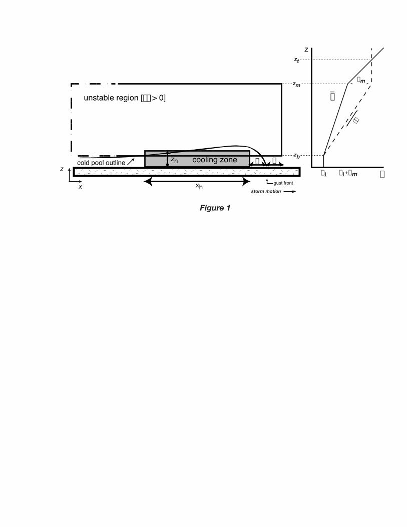
2.2 The moisture parameterization
In this paper, perturbations from any run’s horizontally homogeneous, temporally invariant base
state are denoted with single primes. As described in FT2000, the PM framework (see Fig. 1) is
specifically tailored to the classical squall line’s leading-line and trailing stratiform organization and
mimicks moisture’s first order effects by parameterizing terms representing condensation warming
(Q+) and evaporation cooling (Q−) in the perturbation potential temperature (θ′) equation, viz.
dθ′
dt= Q+ + Q−. (8)
The cooling takes place in a shallow zone in which air is continually relaxed towards a selected
potential temperature perturbation, θ′c, with time scale τc. The zone’s upstream edge is kept a
small distance δ behind the storm’s surface gust front position; this is examined every time step
and shifted if necessary. Q+ is handled as
Q+ = γ∗ max(w, 0), (9)
where w is vertical velocity and γ∗ is the specified parcel potential temperature lapse rate, a function
of height alone. The model subdomain in which γ∗ > 0, termed the “unstable region”, extends to
the downstream lateral boundary but is truncated a small distance ε ahead of the gust front. As
in FT2000, both δ and ε are taken to be 5 km.
7

2.3 Basic model design
FT2000’s PM model implementation was changed in a variety of ways to simplify adjoint construc-
tion. The present model is “quasi-compressible” (Chorin, 1967), discounting the sound speed to
100 m s−1 since larger values produced very similar results at greater expense. The upper and lower
boundaries are rigid, free-slip plates; the horizontal domain is periodic. The latter forces the use
of relatively wider domains though advantageously PM storms tend to develop and mature fairly
quickly.
The two-dimensional (2D) model domain is 550 km wide and 21.2 km deep with horizontal and
vertical grid spacings of ∆x = 1 km and ∆z = 250 m, respectively. Its staggered “C” grid ar-
rangement (Arakawa and Lamb, 1977) places scalar θ′k a distance of 12∆z above and below vertical
velocity points wk and wk+1. The time step ∆t is 0.5 s. Note that “time splitting”, the approach
that integrates acoustically active and inactive terms with different time steps (e.g., Klemp and
Wilhelmson, 1978), was not adopted. We have chosen straightforward over efficient design at this
time.
The modeling system can use either the leapfrog or the Euler-backward schemes, both employing
second order centered differencing for spatial derivatives. The leapfrog is more efficient but its three
time level structure complicates implementation and fidelity assessment of the adjoint model, as well
as interpretation of that model’s intermediate results (see Appendix). These are the strengths of
the two-time level Euler-backward version, though that scheme requires roughly twice the number
of computations and tends to damp high frequency signals (Haltiner and Williams, 1980). The
latter is not a concern; because the model is compressible and not time split, the modes of interest
are actually quite slowly varying. The two versions yield virtually indistinguishable results, for
both forward and reverse integrations (the latter being apparent after adjacent time steps are fused
in the leapfrog model).
8

2.4 Implementing the parameterization in the TLM
The function γ∗ is defined at the w locations at the top and bottom of each grid box, being nonzero
only within the spatially truncated unstable region. When a two time level scheme is employed,
(9) is implemented at time n and scalar spatial location i, k in the nonlinear forward model as
Q+i,k =
∆t
2[max(wn
i,k+1, 0)γ∗k+1 + max(wni,k, 0)γ∗k
]. (10)
That is, the parameterized heating is calculated at the adjacent w locations and then averaged to
the grid box center where θ′ resides. This means the PM model’s discretized latent heating term
(10) is a simple function of two vertical velocities
Q+i,k = F
(wn
i,k+1, wni,k
)making its TLM implementation straightforward. The TLM term, evaluated with respect to the
control run, is
Q′′+i,k = w′′n
i,k+1
∂F
∂wni,k+1
∣∣∣∣∣C
+ w′′ni,k
∂F
∂wni,k
∣∣∣∣∣C
(11)
=∆t
2
[βn
i,k+1w′′ni,k+1γ
∗k+1 + βn
i,kw′′ni,kγ∗k
], (12)
presuming that grid location i, k resides in the unstable region. The subscript C in the first
expression means the term is evaluated for the control run. In the second, β indicates whether
ascent is present in the control run at the given point and time:
βni,k =
{1 wn
i,k > 0;0 otherwise.
Parameterized evaporation cooling in the control run is handled as
Q−i,k = −
(θ′ni,k − θ′c
)τ−1c , (13)
presuming point i, k falls within the spatially confined cooling zone. The TLM version of (13) is
simply
Q′′−i,k = −θ′′ni,kτ−1
c , (14)
at that point1. The position of the cooling zone may shift with time if the control run’s specified
domain translation speed fails to keep the gust front stationary. Our system forces such shifts to
occur at the same time in the TLM and adjoint simulations.1If the leapfrog scheme is employed, the θ′ and θ′′ values used must represent the past time step, n−1, for stability.
9

2.5 Adjoint implementations of the parameterization
Now we turn to the adjoint formulations. Starting with (12) and (14) the adjoint was constructed
by hand transposition following EV’s recipe. First, the salient parts of the TLM prognostic equation
for θ′′, using a two time level scheme and in coded form, are identified:
θ′′n+1i,k = θ′′ni,k +
∆t
2
[βn
k+1w′′ni,kγ∗k+1 + βn
k w′′ni,kγ∗k
]−∆tτ−1
c θ′′ni,k (15)
The TLM variables are next replaced with their adjoint counterparts according to the EV procedure.
This spawns the following three lines of adjoint code
wni,k+1 ← ∆t
2βn
i,k+1θn+1i,k γ∗k+1 (16)
wni,k ← ∆t
2βn
i,kθn+1i,k γ∗k (17)
θni,k ← −∆tτ−1
c θn+1i,k , (18)
where β retains its previous meaning. The leftward directed arrow indicates an assignment to
an equation that may also contain other terms. In building the prognostic expression for wnk , for
example, the right hand side of (17) will be one of the terms included.
Since the adjoint model is being integrated backward in time, time level n+1 “precedes” time level
n. Expression (16) shows that potential temperature sensitivity at grid point i, k and time level
n + 1 (θn+1i,k ) can influence vertical velocity sensitivity at i, k + 1 and time n (wn
i,k+1), but only if
the time n vertical velocity there was positive in the control run. As in the forward model, these
terms affect the adjoint fields only in their respective, designated subdomains.
Automatic adjoint code generators typically produce a string of “line-by-line” code resembling
the above. We note in passing that adjoint code often appears amenable to what we will term
“recombination”, resulting in a more readable and interpretable code, at least when periodic or
solution specified boundary conditions are employed. Expression (16) can be remapped to point
i, k and combined with (17), yielding a single expression added to the right hand side of the w
tendency equation. Indeed, the recombined result, being
wni,k ←
∆t
2βn
i,kγ∗k
[θn+1i,k + θn+1
i,k−1
], (19)
appears to make good physical sense. In the forward TLM (12), the time n vertical velocity
averaged to the scalar location directly affects the temperature perturbation there at time n+1. In
10
the backward propagating adjoint model, the vertical velocity sensitivity at time n is determined
by the time n+1 temperature sensitivities, averaged to the w location. Both are constrained by
the behavior of the control run at time n, through β.
2.6 Verification of the TLM and adjoint
The control/TLM combination may fail to accurately reproduce the alternative run not only owing
to the TLM’s inherent approximations but also due to design and coding errors. Considerable effort
was made to make sure the TLM was free of the latter error sources. The verified TLM model was
then used to vet the correctness of the adjoint model’s coding.
In the course of TLM model validation, the strictly adiabatic discretized model was examined first.
In this configuration, inherent TLM error arises solely due to the neglect of terms beyond first
order in the Taylor expansions. This truncation, however, affects only the advection terms, and
the missing terms themselves are no higher than second order. Indeed, they are nothing other than
easily identified TLM perturbation products.
We tested the adiabatic TLM model code by installing and temporarily reenabling these missing
terms. The output of this “augmented” model should track the discrepancies between the control
and alternative simulations to within roundoff error. This was found to be the case, thereby
validating the adiabatic TLM code itself. Naturally, the perturbation product terms have to be
excluded from the TLM since they cannot be written in matrix form, and thus are not transposable
for use in the adjoint model.
The PM model’s diabatic terms are first order but note (9) is not differentiable at w = 0. Thus,
there is error beyond simple roundoff wherever and whenever the control and alternative simulation
vertical velocities have different signs (as might happen if the updraft boundary were slightly shifted
between two nonlinear simulations, for example). A formulation for (12) that is exact (to within
roundoff error) is
Q′′+i,k =
∆t
2[{max(wn
i,k+1 + w′′ni,k+1, 0)−max(wn
i,k+1, 0)}γ∗k+1
+ {max(wni,k + w′′n
i,k, 0)−max(wni,k, 0)}γ∗k
](20)
11

but this is also not transposable. However, this formulation was used temporarily as a checking
and assessment tool.
The verified TLM model was then used to vet the correctness of the adjoint model’s coding via
the gradient test. For adjoint simulations in general, a control simulation must first be made and
archived. For adjoint validation runs, TLM forecasts are made and archived as well, and those
data are used to calculate ∆J every time step during the backward integration. Recall that ∆J is
temporally invariant when a two time level scheme is employed. In our tests with periodic lateral
boundaries, the Euler backward version of the model can preserve ∆J to sixteen digits when double
precision is used for all reals. As shown by TC, owing to the leapfrog’s three time level structure, ∆J
equivalence can only be shown for the first and final time steps. This equivalency was demonstrated
by the leapfrog version of our adjoint modeling system.
Control run archiving was performed every time step for the simulations shown herein. This requires
a large amount of storage. Significant savings may be realized by archiving at less frequent intervals
(e.g., EV; Langland et al., 1995). In our model, the slow variation of the simulations’ important
modes permits this to be done with very little impact on the computed sensitivities. This will be
exploited in the future.
3 A control run simulation
A simulation was made using the FT2000’s low CAPE (convective available potential energy), low
stability sounding graphically depicted in Fig. 1. The figure also illustrates the path taken by a
parcel rising undiluted from the boundary layer. This parcel’s level of free convection is at zb = 1
km, and its maximum buoyancy (∆m= 3K) is realized at zm = 7 km. Above this point, we presume
the parcel has run out of vapor. Its equilibrium level would reside at zt = 9 km; the CAPE for this
hypothetical parcel is 400 J kg−1.
The base state horizontal wind profile (not shown) consisted of 9.75 m s−1 of wind speed change
over the lowest 3 km, starting with calm conditions at the surface and with zero shear farther aloft.
Since vertical shear vector points eastward, we will refer to the west and east sides of the storm
12

as the “upshear” and “downshear” directions, respectively. The cooling zone was 1.5 km deep and
45 km wide, with θ′c = -4.5K and τc = 600 s. The model was translated eastward at 11.5 m s−1,
effectively rendering the cold pool stationary. The model was run for 9000 s, more than enough
time for the storm to develop and attain a statistically steady structure (see Fovell and Ogura
1988), at least in the vicinity of the convection, without significant artifacts owing to the enforced
periodicity.
Figures 2 and 3 present perturbation fields of potential temperature, horizontal velocity (u′) and
pressure (p′) along with vertical velocity w; for convenience, we have dispensed with the tildes.
Note the u′ field is independent of the reference frame. The principal storm updraft was well
formed by 3000 sec and already leaning rearward (upshear) over the cold pool (Figs. 2a, 3a). The
lower tropospheric flow accelerated upward within the updraft split into two principal branches, the
front-to-rear (FTR) flow which continued rearward, and the forward anvil outflow which overturned
and spread upstream of the storm. The rear inflow current was established beneath the FTR flow,
residing largely in the lower troposphere above the spreading cold pool.
The environment responded to the initiation of convective heating by generating compensating
subsidence which spread in both directions away from the main convecting region as gravity waves.
We will henceforth focus on the eastbound wave which propagated through the storm’s upstream
environment. Figure 3 shows its leading edge was marked by low surface pressure, leaving hori-
zontal airflow that has been accelerated towards (away) from the convection in the lower (upper)
troposphere in its wake. Uninterrupted positive buoyancy concentrated in the middle troposphere
spans that region. This is a combination of the gravity wave’s in situ subsidence warming and
convectively generated warming exported in the forward anvil outflow.
The eastbound wave’s domain-relative propagation speed was ≈ 10 m s−1, making for a 21.5 m s−1
ground-relative motion. The dependence of the phase speed c on H, the vertical dimension of the
diabatic source, is seen in (e.g., Nicholls et al. 1991)
c = u +NH
π, (21)
where u is the mean wind (9.75 m s−1 above the shear layer), N is the Brunt-Vaisalla frequency
(.004 in the base state middle troposphere) and π has its usual meaning. The expected c = 21.5 m
13

s−1 results when H is taken to be 9 km.
4 Examination of forward anvil outflow strength with the adjointmodel
The adjoint model was used to examine the dynamical precursors of the westerly upper tropospheric
forward anvil outflow as it existed at 6000 sec. Basing J on the u field within the subsidence wave’s
leading edge and at the location indicated in Fig. 2b, we made the initial u field a function that
was smoothly tapered from a unit maximum to zero over a 3000 m wide by 800 m deep region.
This effectively makes our J a weighted average of the u field within the specified area2.
In this application, positive ∆J values would represent further intensification of the westerly for-
ward anvil outflow in the aspect region. As revealed by (5), this can be realized by applying
positively (negatively) signed alterations where and when the adjoint model predicts positive (neg-
ative) sensitivity. As would be expected, the individual sensitivities are dynamically consistent
with one another and combine to present a coherent picture. Examining each field’s sensitivity in
isolation, however, helps reveal not only how that field contributes to the whole but also what the
impact of alterations in that field alone might be expected to be.
4.1 Adiabatic adjoint run
Two 3500 sec long backwards runs were made with this J , excluding and including the adjoint’s
diabatic terms. Excluding the moisture parameterization terms renders the adjoint model strictly
adiabatic – and undoubtedly less accurate. Therefore, caution in interpretation is indicated, espe-
cially as sensitivities reach into the unstable region and cooling zone. Still, this simulation illustrates
the adjoint model’s utility as a dynamical tracer in convectively driven flows. The importance of
the diabatic terms is assessed in the next section.
Figures 4 and 5 present contoured adjoint sensitivity fields superimposed upon shaded control run
fields at 4000 sec, 2000 sec into this backward integration. Superposing sensitivity and forward2The initial sensitivity represents an unbalanced jolt and using a smoother initial condition reduces the magnitude
of the resulting acoustic activity.
14

model fields greatly facilitates interpretation. Since the forward anvil outflow and subsidence wave
were thermally driven it is not surprising that sensitivity not only became chiefly concentrated in
the temperature adjoint variable θ but also backtracked towards the actively convecting region as
time rewound3. Positive sensitivity appears in the warmed air just behind the subsidence feature’s
leading edge while negative θ is found immediately above. The former implies that one way to
make the aspect region’s westerly anvil outflow stronger at 6000 sec is to further intensify the warm
anomaly located above x ≈ 280 km at 4000 sec. The latter indicates that the subsequent outflow
could also be enhanced by cooling the neutrally buoyant air located above the warm anomaly.
These operations are sensible, both separately and jointly. Intensifying the already warm air
behind the subsidence wave’s leading edge would make the horizontal buoyancy gradient across that
boundary larger, increasing the local generation of positive horizontal vorticity. As qualitatively
depicted on the figure, the circulatory tendency associated with this vorticity generation would
tend to encourage ascent in the warm anomaly itself as well as westerly flow above and to the east
of it. Cooling the air above the warm anomaly would have the complementary effect of encouraging
subsidence within the anomaly and westerly flow below and to the east of its center. Both of these
westerly enhancements at the present time and place would reasonably lead to subsequent enhanced
westerly flow in the aspect region farther downstream.
Furthermore, note that the largest positive sensitivity resides about 1 km above the location of
the warmest air in the control run at 4000 sec. The adjoint model is indicating that shifting the
present warm and cold anomalies closer together vertically – displacing the cooled (warmed) locale
downward (upward) – would also serve to enhance the subsequent westerly outflow. This should
indeed result because the buoyancy-induced outflows in this case would be concentrated into a still
narrower layer, and would thus be intensified.
In the horizontal velocity field (Fig. 4b), the principal center of positive sensitivity is seen to be
located in the forward anvil outflow at the 8 km level above x ≈ 280 km, where u values in the
control run are positive (westerly). The adjoint model indicates that an increase in the anvil
leading edge westerlies at 4000 sec will result in stronger winds in the forecast aspect region farther3Please note that the contour intervals employed for u, p and w in Figs. 4 and 5 are considerably smaller than
that used for θ. Therefore, perturbations of substantially larger magnitude would need to be applied to these fieldsto accomplish a significant ∆J .
15

downstream 2000 sec later. Thusfar, the adjoint model is providing reasonable, easily interpretable
results.
For vertical velocity (Fig. 5a), the adjoint model again suggests that strenghtening the subsidence
wave at the present time would lead to stronger westerly outflow in the aspect region later. In
the range 270 < x < 290 km, there is positive (negative) sensitivity attached to areas presently
experiencing upward (downward) motions. Comparison with Fig. 4a shows these sensitivities are
in quadrature with the θ field, and consistent with eastward gravity wave phase propagation. Note
some sensitivity has already reached into the main convecting region. There are other features in
the sensitivity field as well, but keep in mind the overall magnitudes of w are extremely small.
The principal signature in the p field (Fig. 5b) is negative sensitivity in the middle troposphere,
above the present surface low center. Perhaps lowering the pressure in the indicated region would
increase the horizontal pressure gradient force exerted on parcels located farther west. This would
accelerate the westerly flow in the forward outflow behind the subsidence wave’s leading edge at
the time depicted. Another interpretation has the adjoint model suggesting that a deepening of the
already present low pressure anomaly now would strengthen the anvil outflow later. As the storm’s
total depth is constrained by the stable stratosphere, this might encourage the westerly flow to be
squeezed into a shallower layer and thereby cause its intensification.
Figures 6 and 7 present the control run and sensitivity fields at 3000 sec. Again, the largest
sensitivities are in the temperature field (Fig. 6a), and are especially concentrated in the warming
near the subsidence feature’s present location. Also notable is the significant negative temperature
sensitivity located farther aloft. The cooling that was present there in the control run resulted
from parcels in the storm’s main updraft (compare with Fig. 7a) overshooting their level of neutral
buoyancy. Note that the forward anvil outflow issues from, and is strongest within, the area between
these sensitivity centers (Fig. 6b). The adjoint model is again indicating that anything that would
serve to make these marked temperature anomalies stronger and closer together now would result
in enhanced westerly flow in the aspect region later.
In addition to the expected positive u sensitivity in the forward anvil, an area of substantial negative
sensitivity has appeared in the lower troposphere (Fig. 7b), straddling the gust front located at x ≈
16

265 km. Across this zone, the storm-relative control run flow switches from weak westerly behind
the gust front to easterly ahead of it. The adjoint model predicts the subsequent forward anvil
outflow would be intensified if that easterly flow were further enhanced (i.e., u′′ < 0). Weakening
the westerlies behind the front are expected to help, for reasons that are less immediately clear.
Perhaps the sensitivities are attempting to impart a downshear tilt on the main storm airflow; such
an orientation would direct more mass into the forward anvil. The effect of including the diabatic
terms on the sensitivity field at this time is discussed below.
The w sensitivity in the main storm updraft (Fig. 7a) seems to suggest alterations that would
shorten but also expand that feature laterally eastward. Either might help shift the cooling resulting
from overshooting towards the east. The negative sensitivity above x = 270 km may be attempting
to widen the subsidence wave’s downdraft (located above x = 275 km) westward. Taken together,
these alterations would sharpen the horizontal w gradients across the east edge of the main storm
updraft, perhaps leading to a stronger overall circulation including enhancement of the forward
anvil’s westerly flow.
The pressure adjoint field (Fig. 7b) suggests a similar interpretation now as at 4000 sec. How-
ever, significant sensitivity has reached the convecting region by this time, rendering the adiabatic
restriction questionable. The diabatic adjoint run is examined next.
4.2 Diabatic adjoint run
Figures 8 and 9 present the sensitivity fields obtained at 3000 sec when the adjoint’s diabatic terms
were enabled4 . Inclusion of the cooling zone term in the backward model had but a very small effect
on the results. As expected, the parameterized warming term, active within the region indicated
on Fig. 8a, exerted a significant impact by this time.
Outside of the unstable region, the temperature sensitivities (Fig. 8a) qualitatively resembled those
from the adiabatic simulation. The diabatic adjoint run, however, put the largest sensitivity on
the east side of the main storm updraft, just inside the unstable region. This warming is colocated
with positive w sensitivity (Fig. 9a), suggesting that enhancing the updraft there (resulting in4Please note that some contour intervals have been increased, particularly for w.
17

more diabatic heating) in the forward model would help increase J . This appears tantamount to
widening the main storm updraft.
Taken together, the u and w sensitivities suggest inducing a clockwise circulation anchored around
z = 6 km above x = 271 km. This circulation would indeed encourage westerly flow into the
forward anvil. As noted above, the adjoint’s diabatic heating term drives the ascending branch of
the circulation. Beyond the unstable region’s east edge, the w and θ sensitivities are in quadra-
ture, likely suggesting eastward gravity wave propagation. The point of largest negative pressure
sensitivity resides near the center of this circulation.
Overall, the importance of the adjoint’s diabatic terms when applied to convectively driven flows
has become clear. Since the westerly outflow is associated with the subsidence wave, anything
that acts to strengthen the latter encourages the former. As the wave itself was triggered by
the convection, wave intensification proceeds from convective enhancement. The adjoint model’s
suggestion of a wider storm updraft perhaps stands in part for an increase in the vertical mass flux.
As additional mass is transported upward, more may be directed into the forward anvil, leading
to a strengthening of the upper tropospheric westerlies so long as the thickness of the outflow
layer is not increased. Recall the sensitivities above and beyond the unstable region appear to be
encouraging a narrowing of that layer.
5 Examination of the lower tropospheric storm inflow with theadjoint model
5.1 Background
Storms exert a substantial impact on their surroundings, including the upstream environment into
which they are propagating. This adjoint investigation was initiated to help explain differences
between PM and traditional cloud model storms with regard to the magnitude and character of
their upstream influence. Figure 10, adapted from FT2000, shows mature phase profiles of ground-
relative horizontal wind taken 20 km ahead of the surface gust front position for three simulations
which shared the same initial wind profile (also shown) and roughly comparable soundings. The
18

explicit moisture benchmark run (grey dashed line) was created with the ARPS5 cloud model (Xue
et al. 2000) using Fovell and Ogura’s (1988; hereafter “FO”) moderate CAPE sounding. The other
two were PM simulations initialized with FT2000’s modified FO environment. The PM simulations
gauge the effect of a “convective sponge”, FT2000’s crude attempt to restrain the upstream influence
(see below); the “basic model” run did not include this extra term. The difference between initial
and disturbed profiles is u′.
All three model storms developed forward anvil outflows (u′ > 0) in the upper troposphere, and mass
continuity dictates there must be compensating inflow enhancement somewhere. The enhancement
in the ARPS case was confined to a relatively shallow midtropospheric layer around 5 km, leaving
the lower troposphere largely unmodified. In the basic PM model simulation, however, the inflow
acceleration extended to the surface, with the maximum increase located very close to the ground.
This is a significant difference. The cloud model storm’s augmented inflow consisted of dry air
which might be expected to weaken the convective intensity. In contrast, much of the basic PM
storm’s enhancement was potentially warm. The vertical shear in contact with the deep convective
updraft differed markedly in the middle troposphere as well. While the low-level shear has the
larger influence on the storm (Rotunno et al. 1988), the middle tropospheric shear is not itself
unimportant (Garner and Thorpe 1992; Fovell and Dailey 1995).
FT2000 focused on the anvil outflow, regarding its significant – and apparently excessive – strength
in the basic PM case as reflecting a fundamental deficiency in the parameterization. Positive
midtropospheric temperature perturbations develop in a mature storm’s trailing region, being a
combination of in situ subsidence and latent heat release along with warming advected rearward by
the FTR flow. In reality, latent heating wanes in the convective cells propagating through this region
because they are being progressively starved of moisture. The moisture parameterization, however,
permits such heating to continue as long as the updraft persists, and of course this heating serves
to maintain the updraft. In this manner, the PM storms’ trailing region temperature perturbations
can become relatively substantial in magnitude. This can be seen for the present PM control run
in Fig. 2.
The midtropospheric warming establishes high perturbation pressure in the upper troposphere5The University of Oklahoma’s Advanced Regional Prediction System.
19

poised above the warmed layer (e.g., Fig. 3). The PM model’s exaggerated rear-side warming
increased the temperature, and thus the pressure, contrast with the forward anvil region. FT2000
hypothesized that if the upper tropospheric horizontal pressure gradient force were reduced, both
the anvil outflow and compensating lower tropospheric inflow would be weakened. To accomplish
this, they fashioned a “convective sponge” to slowly remove positive temperature perturbations in
the trailing region. As suggested by Fig. 10, the sponge could and did reduce the magnitude of both
u′ features in the upstream environment. However, this artificial sponge did not resolve concerns
regarding the inflow’s vertical distribution or the midtropospheric shear. Indeed, decreasing the
circulation’s strength made it more readily apparent that the most important discrepancy lay in
the position, rather than the magnitude, of the maximum enhanced inflow.
5.2 Sensitivity analysis using the adjoint model
What does it take to concentrate the enhanced inflow into the middle troposphere, at least in the
vicinity of the convection? To address this, two separate diabatic adjoint simulations were started at
time 9000 sec with horizontal velocity forecast aspects positioned in the upstream lower and middle
troposphere, respectively (see Fig. 2c). The experiments were designed so that a positive ∆J –
the result of pairing like-signed alterations and sensitivities – would represent a reduction in the
low-level inflow and/or an intensification of the midlevel inflow. The lower tropospheric aspect was
proportional to u itself so ∆J > 0 means weakening the pre-existing easterly wind perturbations.
J was defined as proportional to −u in the middle tropospheric aspect so a positive ∆J increased
those easterlies. Since the adjoint model is linear, the J sign reversal is purely cosmetic.
Though the two adjoint runs were independent, they told the same story6. Again, the temperature
variable quickly came to dominate the results, with both simulations concentrating negative sen-
sitivity in the middle troposphere just upstream of the main storm updraft by 5500 sec (Fig. 11).
The shaded field reveals the control run had some positive θ′ in the sensitive region. A positive ∆J
requires reducing that warming, or even instituting local cooling , at that location and time. Note
the same negative temperature alterations that would decrease the low-level inflow would increase
it at midlevels, thereby accomplishing a shift of the enhanced inflow from near the surface to 5 km,6Implementing both aspects simultaneously yielded very similar results.
20

where the explicit moisture cloud model says it belongs.
These adjoint results motivated Fovell (2002) to revisit the upstream influence issue. There is
indeed weak yet persistent local cooling present just ahead of the convective region in a typical
traditional cloud model simulation (see Fig. 12), something that is absent from its PM counterpart
(Fig. 2). (Note that Fig. 12’s shading scheme deliberately emphasizes these small negative pertur-
bations relative to their positive counterparts.) Fovell (2002) showed the weak upstream cooling
represents the combined effect of cloud water evaporation and the forced ascent of subsaturated,
midtropospheric air encountering the storm updraft. Although undoubtedly exaggerated somewhat
in the 2D geometry, the latter effect is also quite pronounced in three-dimensional simulations as
well (not shown).
The midtropospheric cooling is small in magnitude and quite localized, making it easy to miss amid
the larger and more extensive temperature perturbations of both signs within, above and below
the main updraft. Yet, this subtle perturbation turns out to have had a rather dramatic effect on
the storm inflow structure. Fovell (2002) described the environmental upstream modification as a
gravity wave response to not only the heating but also the cooling occurring in and around the main
storm updraft. The initial heating provokes deep, rapidly propagating subsidence of the kind seen
in Sec. 3; this established the enhanced low-level inflow. The persistent cooling that subsequently
appears during maturity, however, excites a secondary gravity wave response, one characterized
by lower tropospheric ascent. This wave also propagates (albeit more slowly) ahead of the storm,
gently lifting the air approaching the main updraft. As a result, the inflow enhancement is shifted
to the middle troposphere, cooling (and, in the explicit moisture model, moistening) the air in the
process.
Thanks to FT2000’s truncating the unstable region, the PM model is quite capable of handling any
gravity wave response in the upstream environment; what was missing is the cooling . Naturally,
the model has no cloud water to evaporate. However, the original PM framework’s more serious
flaw is that all ascending air in the unstable region is presumed to be saturated and thus generating
condensation warming. In actuality, the air at an updraft’s periphery may represent stable air that
is and remains subsaturated upon ascent, as seen in Fig. 12. Fovell (2002) improved the moisture
parameterization by allowing slowly ascending air to remain subsaturated. This made the PM
21

model results far more comparable to those from traditional cloud models (see his Figs. 13 and 14).
5.3 Discussion
FT2000’s original hypothesis was based on excessive trailing region warming. It is telling that
neither adjoint simulation placed sensitivity in the model storm’s trailing region, at least by 5500
sec (Figs. 11a and 11b). To see whether any sensitivity would appear there at a still earlier time,
the integrations were extended back to 3500 sec. That nothing significant rearward of the main
updraft ever appeared is evidenced by the temperature sensitivity field for the middle tropospheric
aspect (Fig. 11c). This explains why FT2000’s convective sponge failed to resolve the discrepancies
between the PM and explicit moisture model results. As reasonable as their hypothesis may have
seemed, it didn’t describe how the phenomenon in question actually came about in the model. Many
paths to a particular outcome or result are possible, but we are by far most interested in discovering
which path the model took. The usefulness of the adjoint model as a backwards dynamical tracer
is hereby demonstrated.
The success of the improved moisture parameterization encouraged us to consider a more sophis-
ticated adjoint formulation, one that has explicit moisture but the bare minimum of complexity.
Figure 13 presents results from a “no-cloud cloud model” (NCCM), which combines the PM cooling
zone with a typical cloud model saturation adjustment scheme. However, cloud water is removed
as it is generated, so only the adjoint of the saturation adjustment itself is necessary. Cloud wa-
ter evaporation is missing from the model, but analysis suggests its contribution is not necessary.
Starting with the FO sounding, the NCCM model storm easily generates weak but persistent cool-
ing upstream of the convective region and the elevated upstream inflow it provokes. Figure 13b
presents the temperature sensitivity field at 5500 sec, resulting from the lower tropospheric J con-
sisting of horizontal velocity positioned as shown in Fig. 13a. The results confirm those obtained
from the PM model and demonstrate that much of what makes traditional cloud models (and their
adjoints) so very complicated can sometimes be neglected.
22

6 Summary
The adjoint of a parameterized moisture (PM) convection model was described and tested. Ad-
joint models are useful for tracing features back to their dynamical origins, facilitating hypothesis
construction and testing. However, such models can be difficult to construct and are based on
sometimes worrisome linearity assumptions. Certainly, cloud microphysics, including the satura-
tion process, are very complicated, involving numerous nonlinearities and interactions as well as
binary switches. The PM framework dramatically reduces the model’s complexity by specifying
the location and magnitude of evaporation cooling and by making latent heating conditionally pro-
portional to vertical velocity. Its adjoint is simple and linear, and can be implemented with little
error.
However, the PM adjoint’s usefulness is limited if the moisture parameterization cannot produce
reasonable results. Naturally, there are many things a PM model can never simulate. However,
our previously cited reservations (Fovell and Tan 2000) concerned the degree of influence exerted
by PM model storms on the environments into which they are propagating. Compared to explicit
moisture cloud models, PM convection generated overly strong forward anvil outflows and put the
compensating tropospheric inflow far too close to the surface. The strength and nature of the
enhanced upstream inflow is very different for PM and explicit moisture storms, at least in the
immediate vicinity of the convection.
Fovell and Tan (2000) advanced a hypothesis to explain the discrepancies between the models
but the “fix” that hypothesis motivated did not appreciably improve the results. The PM model
adjoint results described herein pointed to an entirely different, and previously overlooked, cause.
Motivated by these results, Fovell (2002) revisited the upstream influence issue. Thus, in this
application, the adjoint proved to be instrumental in disproving one hypothesis and suggesting
another, leading to an improvement of both the PM model framework and our understanding of
convective storms. The PM results also motivated a more sophisticated, but still relatively simple,
adjoint that explicitly includes vapor but ignores water following condensation. Further applications
of the PM and the “no-cloud cloud model” adjoints will be explored in the future.
Acknowledgments. This work was supported by NSF grant ATM-0139284.
23

Appendix
Issues faced when using the three time level leapfrog (LF) scheme in an adjoint modeling system are
demonstrated using a simple advection equation for TLM variable u′′. This discussion represents
an amplification of Talagrand and Courtier’s (1987) Appendix C. When alterations to a constant
advection speed Cx are ignored, the TLM equation is
∂u′′
∂t= −Cx
∂u′′
∂x. (22)
Discretization using leapfrog time and center space differencing yields
u′′n+1i = u′′
n−1i − Cx2∆t
2∆x
[u′′
ni+1 − u′′
ni−1
]. (23)
The initial condition (IC) for the forward model is placed in u′′0i for any or all i. Integration
commences with a forward (Euler) time step, coded as
u′′1i = u′′
0i −
Cx∆t
2∆x
[u′′
0i+1 − u′′
0i−1
]. (24)
For time steps n = 1, N -1, the standard LF is coded as:
u′′n+1i = u′′
n−1i − Cx2∆t
2∆x
[u′′
ni+1 − u′′
ni−1
]. (25)
Time step N -1 concludes with the final forecast representing time N .
Thus, for all time steps except the first, the LF scheme fuses information from time levels n − 1
and n into the forecast for time n + 1 (Fig. A-1, upper panel). The adjoint of (24), proceeding
in reverse, unravels this by placing information from time n + 1 into both the n and n − 1 time
levels. In other words, the n+1 time level was influenced by two prior times in the forward model,
so in the reverse model it influences two earlier times (Fig. A-1, lower panel). This is seen in the
following adjoint code, used for time steps n=N -1. . . 1:
un−1i ← un+1
i (26)
uni+1 ← −Cx
2∆t
2∆xun+1
i (27)
uni−1 ← +Cx
2∆t
2∆xun+1
i . (28)
24

The backward integration concludes with the adjoint of (24), which is:
u0i ← u1
i (29)
u0i+1 ← −Cx
∆t
2∆xu1
i (30)
u0i−1 ← +Cx
∆t
2∆xu1
i . (31)
All information is finally combined into the single, final time level.
The chief disadvantage of LF time differencing is that adjacent times must be combined to obtain
a complete adjoint sensitivity field for at any intermediate time step between the first and final
times. This is illustrated in Fig. A-2 for the present example. Consider an adjoint IC consisting
of a single grid point (i.e., uNi ), indicated by the white dot labeled “0”. Stepping from time step
N to N -1 with (26)-(28), this IC leads to information being placed into three time/space locales:
uN−1i+1 , uN−1
i−1 and uN−2i . The points involved in this first adjoint operation bear the label “1” in Fig.
A-2. The next time step affects the locales marked “2”. The time/space locale (i,N − 2) is being
modified for the second time, so it bears both labels. At the conclusion of the third adjoint time
step, the IC’s influence has spread to the locales designated “3”.
Though the example ceases at this point, the staggering has become obvious. It is clear that in
order to retrieve a full intermediate field, two adjacent time levels would have to be combined.
Further, this temporal-spatial separation isn’t finally cured or “congealed” until the very last LF
operation, the Euler step. It is that operation that finally stitches the odd and even time level
fields together. This represents a significant limitation that is not shared by models employing two
time level schemes.
25
References
Arakawa A, Lamb V (1977): Computational design of the basic dynamical processes of the UCLA
general circulation model. Methods Comput Phys 17: 174-267.
Cacuci DG, Hall MCG (1984): Efficient estimation of feedback effects with application to climate
models. J Atmos Sci 41: 2063-2068.
Chorin AJ (1967): A numerical method for solving incompressible viscous flow problems. J Comput
Phys 2: 12-16.
Errico RM (1997) What is an adjoint model? Bull Amer Meteor Soc 78: 2577-2591.
Errico RM, Vukicevic T (1992) Sensitivity analysis using an adjoint of the PSU-NCAR mesoscale
model. Mon Wea Rev 120: 1644-1660.
Fovell RG (2002) Upstream influence of numerically simulated squall-line storms. Quart J Roy
Meteor Soc 128: 893-912.
Fovell RG, Dailey PS (1995): The temporal behavior of numerically simulated multicell-type storms,
Part I: Modes of behavior. J Atmos Sci 52: 2073-2095.
Fovell RG, Ogura Y (1988): Numerical simulation of a midlatitude squall line in two dimensions.
J Atmos Sci 45: 3846-3879.
Fovell RG, Tan P-H (2000) A simplified squall-line model revisited. Quart J Roy Meteor Soc 126:
173-188.
Garner, ST, Thorpe AJ (1992): The development of organized convection in a simplified squall-line
model. Quart J Roy Meteor Soc 118: 101-124.
Ghil M, Ide K, Bennett AF, Courtier P, Kimoto M, Sato N, editors (1997) Data Assimilation in
Meteorology and Oceanography: Theory and Practice. Tokyo: Meteorological Society of Japan
and Universal Academy Press, 496 pp.
26

Haltiner GJ, Williams RT (1980): Numerical Weather Prediction and Dynamic Meteorology. New
York: Wiley, 477 pp.
Klemp JB, Wilhelmson RB (1978): The simulation of three-dimensional convective storm dynamics.
J Atmos Sci 35: 1070-1096.
Langland RH, Elsberry RL, Errico RM (1995): Evaluation of physical processes in an idealized
extratropical cyclone using adjoint sensitivity. Quart J Roy Meteor Soc 121: 1349–1386.
Langland RH, Gelaro R, Rohaly GD, Shapiro MA (1999): Targeted observations in FASTEX:
Adjoint-based targeting procedures and data impact experiments in IOPs-17 and 18. Quart J Roy
Meteor Soc 125: 3241-3270.
Lorenz EN, Emanuel KA (1998): Optimal sites for supplementary weather observations: Simula-
tions with a small model. J Atmos Sci 55: 399-414.
Nicholls ME, Pielke RA, Cotton WR (1991): Thermally forced gravity waves in an atmosphere at
rest. J Atmos Sci 48: 1869-1884.
Park SK, Droegemeier KK (1999): Sensitivity analysis of a moist 1-D Eulerian cloud model using
automatic differentiation. Mon Wea Rev 127: 2128-2142.
Park SK, Droegemeier KK (2000): Sensitivity analysis of a 3D convective storm: Implications for
variational data assiimilation and forecast error. Mon Wea Rev 128, 140-159.
Rabier F, Klinker E, Courtier P, Hollingsworth A (1996): Sensitivity of forecast errors to initial
conditions. Quart J Roy Meteor Soc 122: 121-150.
Reed RJ, Kuo Y-H, Albright MD, Gao K, Guo Y-R, Huang W (2001): Analysis and modeling of
a tropical-like cyclonein the Mediterranean Sea. Meteor Atmos Phys 76: 183-202.
Rosmond TE (1997): A technical description of the NRL adjoint modeling system. Naval Research
Laboratory, Monterey, CA, publication NRL/MR/7532/97/7230.
27

Rotunno R., Klemp JB, Weisman ML (1988): A theory for strong, long lived squall lines. J Atmos
Sci 45: 463-485.
Talagrand O, Courtier P (1987) Variational assimilation of meteorological observations with the
adjoint vorticity equation. I: Theory. Quart J Roy Meteor Soc 113: 1311-1328.
Xu Q (1996): Generalized adjoint for physical processes with parameterized discontinuities. Part
I: Basic issues and heuristic examples. J Atmos Sci 53: 1123-1142.
Xue M, Droegemeier KK, Wong V (2000): The Advanced Regional Prediction System (ARPS) – a
multi-scale nonhydrostatic atmospheric simulation and prediction model. Part I: Model dynamics
and verification. Meteor Atmos Phys 75: 161-193.
Zou X (1997): Tangent linear and adjoint of “on/off” processes and their feasibility for use in
4-dimensional variational data assimilation. Tellus 49A: 3-31.
28

Figure captions
Figure 1 - Schematic model illustrating PM model design. Fovell and Tan’s (2000) low CAPE
sounding is depicted at right. See text.
Figure 2 - Perturbation fields of potential temperature θ′ (shaded; K) and horizontal velocity u′ (3
m s−1 contours) for the control run. The zero contour is suppressed. Only a portion of the domain
is shown.
Figure 3 - As in Fig. 2, but for perturbation pressure p′ (shaded; hPa) and vertical velocity w (3
m s−1 contours). Additionally, the -1 m s−1 vertical velocity contour has been included.
Figure 4 - Control (shaded) and adjoint sensitivity (contoured) fields at 4000 sec: (a) perturbation
potential temperature field θ (.05 m s−1 K−1 contours); (b) horizontal velocity field u (.0075
[nondimensional] contours). Control field is full, storm-relative u rather than u′. Shown in panel
(a) is the circulatory tendency implied by the adjoint sensitivity field.
Figure 5 - As in Fig. 4, but showing: (a) vertical velocity sensitivity field w (.001 [nondimensional]
contours); (b) perturbation pressure sensitivity field p (.002 m s−1 hPa−1 contours).
Figure 6 - As in Fig. 4, but at 3000 sec. Temperature sensitivity contour interval is .025 m s−1
K−1; for the horizontal velocity sensitivity it is .005 (nondimensional).
Figure 7 - As in Fig. 5, but at 3000 sec. Vertical velocity sensitivity contoured at .002 (nondimen-
sional) intervals; for the pressure sensitivity it is .001 m s−1 hPa−1.
Figure 8 - As in Fig. 6, but for the diabatic adjoint run. Temperature sensitivity contour interval
is .03 m s−1 K−1; for the horizontal velocity sensitivity it is .005 (nondimensional).
Figure 9 - As in Fig. 7, but for the diabatic adjoint run. Vertical velocity sensitivity contour interval
is .003 (nondimensional); for the pressure sensitivity it is .0015 m s−1 mb−1).
Figure 10 - Instantaneous mature phase vertical profiles of ground-relative horizontal wind, taken
at a location 20 km upstream of the surface gust front position for an ARPS model simulation
29

and PM model runs made without and with a “convective sponge” term. Also shown is the initial,
undisturbed wind profile. The FO-MOD sounding was derived from Fovell and Ogura’s (1988;
“FO”) initial environment, used in the ARPS run. Note that the PM runs did not employ the
sounding in Fig. 1. After Fovell and Tan (2000).
Figure 11: Control (shaded) and adjoint sensitivity (contoured) fields of perturbation potential
temperature for: (a) the lower tropospheric aspect at 5500 sec; (b) the middle tropospheric aspect
at 5500 sec; and (c) the middle tropospheric aspect at 3500 sec. See Fig. 2c for locations of these
aspects.
Figure 12 Perturbation fields of potential temperature (shaded; K) and horizontal velocity (3 m
s−1 contours) for a typical explicit moisture simulation, made using ARPS and the FO sounding.
Updraft outline is w = 1.75 m s−1. Color table chosen emphasizes the small cooling residing at
and upstream of the leading edge.
Figure 13 Control (shaded) and adjoint sensitivity (contoured) fields from a no-cloud cloud model
(NCCM) simulation made with the FO sounding, showing: (a) perturbation horizontal velocity with
initial forecast location superposed; and (b) perturbation potential temperature and sensitivity (0.1
K s m−1 contours).
Figure A-1: Schematic illustrating the leapfrog scheme in the forward TLM and adjoint models.
Figure A-2: Schematic illustrating why odd and even time steps in the adjoint integration do not
separately yield full solutions for steps between the initial and final times when the leapfrog scheme
is employed.
Mailing address:
Prof. Robert G. Fovell
Department of Atmospheric Sciences
University of California, Los Angeles
405 Hilgard Ave
Los Angeles, CA 90095-1565
30
unstable region [g* > 0]
cooling zonecold pool outline
xh
d ezhz
x
q
z
gust frontstorm motion
zb
zm
zt
Dm_
g*
qq1 q1+Dm
Figure 1

W
C
C
W
250 300
5
10
5
10
5
10
(a)
(b)
(c)
t = 3000 sec
t = 6000 sec
t = 9000 sec
perturbations of horizontal velocity (contoured) and potential temperature (shaded)
z (k
m)
x (km)
Figure 2
Sec. 4 aspect
Sec. 5 aspects

250 300
5
10
5
10
5
10
(a)
(b)
(c)
t = 3000 sec
t = 6000 sec
t = 9000 sec
vertical velocity (contoured) and perturbation pressure (shaded)
z (k
m)
x (km)
L
H
Figure 3

(a) potential temperature perturbation and sensitivity
(b) horizontal velocity and sensitivity
t = 4000 sec
t = 4000 sec
250 300
5
10
250 300
5
10
Figure 4
x (km)
z (k
m)
z (k
m)
aspectlocation

250 300
5
10
250 300
5
10
(a) vertical velocity and sensitivity
(b) pressure perturbation and sensitivity
t = 4000 sec
t = 4000 sec
Figure 5
x (km)
z (k
m)
z (k
m)
L
L
H

(a) potential temperature perturbation and sensitivity
(b) horizontal velocity and sensitivity
t = 3000 sec
t = 3000 sec
250 300
5
10
250 300
5
10
Figure 6
x (km)
z (k
m)
z (k
m)

(a) vertical velocity and sensitivity
(b) pressure perturbation and sensitivity
t = 3000 sec
t = 3000 sec
250 300
5
10
250 300
5
10
Figure 7
x (km)
z (k
m)
z (k
m)
LL
H

(a) potential temperature perturbation and sensitivity
(b) horizontal velocity and sensitivity
t = 3000 sec
t = 3000 sec
250 300
5
10
250 300
5
10
Figure 8
x (km)
z (k
m)
z (k
m)
unstable region

(a) vertical velocity and sensitivity
(b) pressure perturbation and sensitivity
t = 3000 sec
t = 3000 sec
250 300
5
10
250 300
5
10
Figure 9
x (km)
z (k
m)
z (k
m)
L
L
H

0
2
4
6
8
1 0
1 2
z (k
m)
- 2 0 - 1 0 0 1 0 2 0 3 0 4 0u (m/s)
Upstream ground-relative horizontal winds(vertical sections taken 20 km ahead of line)
PM model / FO-MOD(basic model)
PM model / FO-MOD(with convective sponge)
ARPS model / FO
Initial profile
Figure 10

5
10
5
10
potential temperature perturbation and sensitivity(a) lower tropospheric aspect started at 9000 sec
(b) middle tropospheric aspect started at 9000 sec
t = 5500 sec
Figure 11
5
10
250 300
potential temperature perturbation and sensitivity(c) middle tropospheric aspect started at 9000 sec
t = 3500 sec
main updraft
main updraft
main updraft
x (km)
z (k
m)

280 320300 340
3
6
9
t = 9720 sec
<<< -1.0 0 1.0 2.0 3.0 4.0 5.0 6.0 >>>
z (k
m)
x (km)
ARPS potential temperature (shaded)and horizontal velocity (contoured) perturbations
updraft outline
Figure 12

(a) NCCM perturbation horizontal velocity and forecast aspect
(b) NCCM perturbation potential temperature and sensitivity
t = 7200 sec
t = 5500 sec
200 250
5
10
200 250
5
10
x (km)
z (k
m)
z (k
m)
updraft outline
Figure 13

n+1nn-1
n+1nn-1
leapfrog in forward model (n=1...N-1)
leapfrog in adjoint model (n=N-1...1)
Figure A-1

time level
N
N-1
N-2
N-3
N-4
i-1i-2i-3 i i+1 i+2 i+3 i+4 i+5i-4i-5
grid index
Figure A-2
0
1 1
122 2
3 3
3 3 3
2 3 2 3