convection in a parameterized and superparameterized model

Convection in a Parameterized and Superparameterized Model and Its Rolein the Representation of the MJO

HONGYAN ZHU AND HARRY HENDON

Bureau of Meteorology, CAWCR, Melbourne, Victoria, Australia

CHRISTIAN JAKOB

School of Mathematical Sciences, Monash University, Melbourne, Victoria, Australia

(Manuscript received 3 February 2009, in final form 30 March 2009)

ABSTRACT

The behavior of convection and the Madden–Julian oscillation (MJO) is compared in two simulations from

the same global climate model but with two very different treatments of convection: one has a conventional

parameterization of moist processes and the other replaces the parameterization with a two-dimensional

cloud-resolving model, the so-called superparameterization. The different behavior of local convection and

the MJO in the two model simulations reveals that the accurate representation of the following characteristics

in the modes of convection might contribute to the improvement of the MJO simulations: (i) precipitation

should be an exponentially increasing function of the column saturation fraction, (ii) heavy precipitation

should be associated with a stratiform diabatic heating profile, and (iii) there should be a positive relationship

between precipitation and surface latent heat flux.

1. Introduction

The Madden–Julian oscillation (MJO) is the domi-

nant mode of tropical intraseasonal variability (e.g.,

Madden and Julian 1994) and it affects a wide range of

tropical weather including the onset and breaks of

the Indian and Australian summer monsoons (e.g.,

Yasunari 1979; Hendon and Liebmann 1990; Wheeler

and McBride 2005; Goswami 2005) and the formation

of tropical cyclones (e.g., Liebmann et al. 1994; Bessafi

and Wheeler 2006). The MJO is a major modulator of

tropical diabatic heating and as such plays an important

role in driving teleconnections throughout the tropics

and into the extratropics (e.g., Weickmann et al. 1985).

Furthermore, the MJO is associated with the triggering

and termination of some El Nino events (e.g., Kessler

et al. 1995; McPhaden 2008; Hendon et al. 2007).

Given the prominent role of the MJO with regard to

global weather and climate, it is imperative that global

climate models (GCMs) adequately simulate the MJO in

order to faithfully represent the full spectrum of climate

variability. However, GCMs continue to have difficulty

in simulating many of the important characteristics of

the MJO. Typically, model MJOs are too weak, espe-

cially the convective component, and they propagate

eastward too fast (e.g., Hayashi and Sumi 1986; Lau et al.

1988; Slingo et al. 1996; Maloney and Hartmann 2001).

Although some recent progress in the simulation of

the MJO has been reported (e.g., Waliser et al. 2003;

Zhang et al. 2006), the state-of-the-art coupled ocean–

atmosphere GCMs participating in the Intergovernmental

Panel on Climate Change (IPCC) Fourth Assessment

Report (AR4) all continue to have significant problems

in representing the MJO (Lin et al. 2006).

The simulation of the MJO in GCMs has shown great

sensitivity to the details of convective parameterization

(e.g., Wang and Schlesinger 1999; Maloney and Hartmann

2001), which thus points to the representation of trop-

ical convection as being an important contributor to

the generally poor simulations of the MJO in current

GCMs. Diagnosing the problems of a particular con-

vective parameterization that leads to the poor simula-

tion of the MJO has, however, proved to be a difficult

challenge. To put another way, it is not obvious which

aspects of convective behavior need to be faithfully

Corresponding author address: Dr. Hongyan Zhu, Bureau of

Meteorology, CAWCR, GPO Box 1289, Melbourne VIC 3001,

Australia.

E-mail: [email protected]

2796 J O U R N A L O F T H E A T M O S P H E R I C S C I E N C E S VOLUME 66

DOI: 10.1175/2009JAS3097.1

� 2009 American Meteorological Society

represented by a parameterization in order to ade-

quately represent the MJO (and other modes of large-

scale organized convection). One common finding from

modeling experiments is the sensitivity of the simulated

MJO to threshold conditions for the onset of convection:

higher thresholds typically result in better organized

and stronger MJOs [e.g., Tokioka et al. (1988), using

a minimum entrainment threshold, and Wang and

Schlesinger (1999), with a relative humidity threshold in

the convection scheme]. However, this sensitivity is not

universal; the results of Maloney and Hartmann (2001)

suggest rather that it is the realistic simulation of the

mean humidity above the boundary layer and its evo-

lution through the life cycle of the MJO (e.g., as a result

of evaporation of convective precipitation) that is cru-

cial for a faithful simulation of the MJO.

To build on sensitivity studies such as those by

Maloney and Hartmann (2001), we will examine some

possible critical dependencies for tropical convection on

a variety of parameters, including column-integrated

humidity (e.g., Bretherton et al. 2004) and surface

moisture fluxes (e.g., Raymond et al. 2003), that may be

related to the evolution of the MJO. Rather than con-

duct sensitivity experiments with a single convection

parameterization, we will make use of two simulations

from the same GCM but with two very different treat-

ments of convection and very different simulations of

the MJO. Our focus will be on diagnosing the local

controls of tropical convection and associated rainfall as

resolved on GCM grids, which is thus naturally compa-

rable to observed behavior as resolved, for instance, by

global satellite products with similar resolutions. The

aim of this analysis is to provide a better understanding

of those aspects of convective behavior that are critical

for a proper simulation of the MJO.

2. CAM and SP-CAM models

Our analysis is based on Atmospheric Model Inter-

comparison Project (AMIP)-style simulations of the

Community Atmosphere Model (CAM), version 3

(Collins et al. 2004) and the ‘‘superparameterized’’

version of the same model (SP-CAM), which were

performed at Pacific Northwest National Laboratories

(Marchand et al. 2009). The standard CAM simulation

uses the Zhang and McFarlane (1995) method for con-

vective parameterization, which is a mass flux scheme

with a closure based on the assumption that convection

consumes large-scale convective available potential en-

ergy (CAPE) and acts to return the atmosphere to a

neutrally buoyant state over a given convective adjust-

ment time scale. The SP-CAM is based on the multiscale

modeling framework (MMF), which is a new approach

to climate modeling (Grabowski 2001; Khairoutdinov

and Randall 2001; Khairoutdinov et al. 2005) in which

cloud processes are treated more explicitly by replacing

the parameterizations of a GCM with a 2D cloud

system–resolving model at each grid point of the GCM.

Details of some comparisons between the simula-

tions using the CAM and SP-CAM can be found in

Khairoutdinov et al. (2005) and DeMott et al. (2007).

Some improvements of the simulated tropical climate in

SP-CAM over CAM reported in these studies are 1) an

improved diurnal cycle of precipitation over land, 2)

a more realistic distribution of cirrus cloudiness, 3) a

better simulation of heavy rainfall, and 4) a more real-

istic relationship among precipitation and lower- and

upper-level humidity. Although many aspects of the

climate related to clouds and precipitation are reported

to have improved in the SP-CAM over the standard

CAM, there are still several problems in the SP-CAM

simulation that require explanation. These include a

high rainfall bias in the western Pacific, too high a zonal

wind variability in the tropics, an overactive Indian

monsoon, and a failure to simulate light rain rates.

One important result from the study of Khairoutdinov

et al. (2005) is that the SP-CAM produces a more real-

istic MJO, whereas the MJO is completely absent from

the CAM. Thus, the simulations with the SP-CAM and

CAM provide a potentially useful test bed to explore the

link between the behavior and controls of subgrid-scale

convection and the ability to simulate the MJO. We will

assess and compare the behavior of tropical convection

in the two simulations, with the aim of elucidating those

aspects of convection that might be associated with an

improved simulation of the MJO. We also compare the

model results with observations and to some previously

published studies based on observed behavior.

The observation datasets for verification in this pa-

per are the Global Precipitation Climatology Project

(GPCP) daily precipitation with 18 resolution (Adler

et al. 2003); the daily mean latent heat flux from the

Woods Hole Oceanographic Institution (WHOI) Ob-

jectively Analyzed Air–Sea Fluxes Project (OAFlux; Yu

et al. 2008), also with 18 resolution; and the 40-yr Eu-

ropean Centre for Medium-Range Weather Forecasts

(ECMWF) Re-Analysis (ERA-40) of winds, tempera-

ture, and moisture fields with 2.58 resolution (Uppala

et al. 2005). ERA-40 reanalyses are from a data assim-

ilation system and therefore contain an optimal blend of

model results and observations. For simplicity we will

refer to the reanalyses as observations, acknowledging

that they are not based on observations alone. Our re-

sults will show, however, that it is unlikely the model

shortcomings we identify are an artifact of the use of

ERA-40. For model simulations and observations, we

SEPTEMBER 2009 Z H U E T A L . 2797

use daily data for the period July 1998–June 2002 (the

period of available model simulations). The model

output is available on a 2.58 3 2.08 grid.

3. Results

a. Initial assessment of the MJO

The simulation of the MJO in the two models is ini-

tially assessed using wavenumber–frequency spectral

analysis (e.g., Salby and Hendon 1994). The analysis

is applied to daily mean rainfall and zonal wind at

850 hPa (hereafter U850) for the region 148S to 148N,

and, to focus on the MJO, we display the power for the

equatorially symmetric components (e.g., Wheeler and

Kiladis 1999). The observed MJO is characterized by a

distinct spectral peak at eastward wavenumber 1 for

zonal wind and eastward wavenumbers 1–3 for precipi-

tation at periods of 30–90 days (Fig. 1), which is consis-

tent with observational analyses using longer records

(e.g., Salby and Hendon 1994). The SP-CAM (Figs. 2a,b)

exhibits a strong peak at MJO wavenumbers and fre-

quencies for both U850 and precipitation. In fact, the

peak power for U850 at eastward wavenumber 1 and a

50-day period is about 4 times greater than the observed,

whereas the equivalent spectral peak for rainfall is

about double of the observed value, which is somewhat

unique for modern climate models (e.g., Maloney and

Hartmann 2001; Zhang et al. 2006). Hence, the SP-CAM

exhibits a very clear and pronounced MJO signal. East-

ward power and westward power are both stronger in the

SP-CAM compared to observation, but the ratio be-

tween eastward and westward power in SP-CAM is

similar to that in observation. On the other hand, CAM

has almost equal power in eastward and westward power,

and the spectra appear red in frequency, with maximum

power occurring at the lowest frequency and with no

intraseasonal peak. Hence, we infer that the MJO is

completely absent in the CAM simulation (Figs. 2c,d).

b. Relationship between precipitation andcolumn-integrated humidity

Precipitation over the tropical oceans is observed to

strongly vary with tropospheric humidity (e.g., Bretherton

et al. 2004; Sherwood 1999). In particular, Bretherton

et al. (2004) have highlighted a quasi-exponential re-

lationship between the precipitation rate and column

saturation fraction (hereafter saturation fraction).

Raymond (2007), for instance, found that in a simple

model the sensitivity of the convective parameterization

to saturation fraction plays a key role in determining the

time and space scales of tropical convective variability.

In particular, the ability of the model to exhibit orga-

nization at time and space scales associated with the

MJO was shown to be sensitive to the humidity state of

the atmosphere as represented by saturation fraction.

Based on these studies, we begin our examination of

convection behavior in the CAM and SP-CAM by in-

vestigating their representation of the relationship be-

tween saturation fraction and tropical precipitation.

Daily values of saturation fraction are computed as

r 5 W/W*, where W and W* are the column-integrated

water vapor mixing ratio and column-integrated satu-

rated water vapor mixing ratio, respectively. Figure 3a

shows observed and simulated daily mean precipitation

in 5% bins of saturation fraction for tropical ocean

points across the western Pacific/Indian Ocean warm-

pool region (128S–128N, 608–1808E). The strong sensi-

tivity of rainfall to saturation fraction as diagnosed by

Bretherton et al. (2004) is reproduced here using differ-

ent observed rainfall, moisture, and temperature data-

sets. In particular, precipitation is observed to become

nonzero at about 0.5 saturation fraction and then in-

creases nearly exponentially with saturation fraction until

a slight flattening occurs above 0.8 saturation fraction.

In the CAM simulation, the onset of precipitation

occurs at a lower saturation fraction than observed (less

than 0.4 as compared to greater than 0.5 for observed),

with most of the increase in precipitation occurring in

the range of 0.4 and 0.75, after which rainfall does not

increase further with increases in saturation fraction

(or even tails off). The shape of the rainfall-saturation

fraction relationship in the CAM is, however, similar to

the observed, although it is shifted to lower saturation

fraction for the equivalent rainfall rate by about 0.2.

The SP-CAM shows a very different behavior to the

CAM. Significant rainfall does not occur until the satu-

ration fraction exceeds 0.6, followed by a steeper-than-

observed increase of rainfall with saturation fraction

that continues up to the highest rainfall rates, where the

maximum rainfall rate at 0.95 saturation fraction is more

than double the observed rate.

The frequency of occurrence of saturation fraction is

shown in Fig. 3b. The observed distribution is strongly

peaked with the mode near 0.7–0.75, with a sharp de-

cline toward higher saturation fraction (very few oc-

currences greater than 0.9) and a long tail toward lower

saturation fraction. The CAM displays a much more

symmetric and narrower distribution that is peaked at

about 0.55, with very few occurrences of saturation

fraction greater than 0.7, which is near the mode of the

observed distribution. This narrower and drier distri-

bution in the CAM might be indicative of convection

being triggered too easily, thereby drying the atmo-

sphere before it can reach saturation values of 0.7 and

greater. The shape of the frequency distribution for the

SP-CAM is closer to the observed, with a mode of about


0.75, but the occurrence of saturation fraction greater

than 0.75 drops off much more slowly than observed,

displaying a significant number of occurrences of satu-

ration fraction greater than 0.9. There are also fewer

occurrences of dry states (saturation fraction less than

0.5) than observed. Thus, the SP-CAM may have con-

vection behavior opposite to that of the CAM, with

convection being triggered only when the atmosphere

has reached higher than observed saturation fraction.

This analysis of rainfall rate versus saturation fraction

in the two simulations is consistent with the recent study

of DeMott et al. (2007), who computed the probability

distribution function of daily mean rainfall for 3 months

in three geographic locations from simulations with the

FIG. 1. The symmetric precipitation and U850 space–time power spectrum for observation for latitudes from 148S

to 148N. Contour interval (CI) for precipitation power is 0.004 mm2 day22, with additional contours of 0.002 and

0.001 mm2 day22; CI for U850 power is 0.02 m2 s22, with additional contours of 0.005 and 0.001 m2 s22. Superimposed

are the theoretical shallow-water dispersion curves for the equatorial Rossby and Kelvin waves with equivalent

depths of 25 and 50 m.


CAM and SP-CAM. They found that CAM produces too

much light-to-moderate rainfall and not enough heavy

rainfall, whereas the SP-CAM underestimates rain con-

tributions from the lightest rainfall rates but more real-

istically simulates more intense rainfall events. From our

analysis it appears that these more realistic high-intensity

rainfall events occur in too moist of an atmosphere.

c. Relationship between precipitation and verticalprofile of humidity

To better understand the differing relationships be-

tween rainfall rate and saturation fraction in the SP-CAM

and CAM simulations, we investigate the relationship

between rainfall rate and the vertical profile of humidity

(mixing ratio). To do so, we calculate humidity anoma-

lies (anomalies formed by removing the climatologically

seasonal cycle and mean value over the 4 years) as a

function of rainfall intensity. Instead of choosing arbi-

trary thresholds, we divide the rainfall rate into 10 equal

bins (deciles) to represent the intensity of precipitation

rate below, at, and above the average value. Note that

the decile divisions are specific to each of the three

rainfall datasets (GPCP, CAM, and SP-CAM) because

each has a different rainfall distribution. The threshold

FIG. 2. As in Fig. 1, but for the (a),(b) SP-CAM and (c),(d) CAM simulations.

FIG. 3. (a) Mean daily precipitation composited into 5% bins of saturation fraction for tropical ocean grid points in

the west Pacific and Indian Ocean warm-pool region (128S–128N, 608–1808E) for SP-CAM, CAM, and observation.

(b) Ratio of number of observations in each bin to the total number of data points.


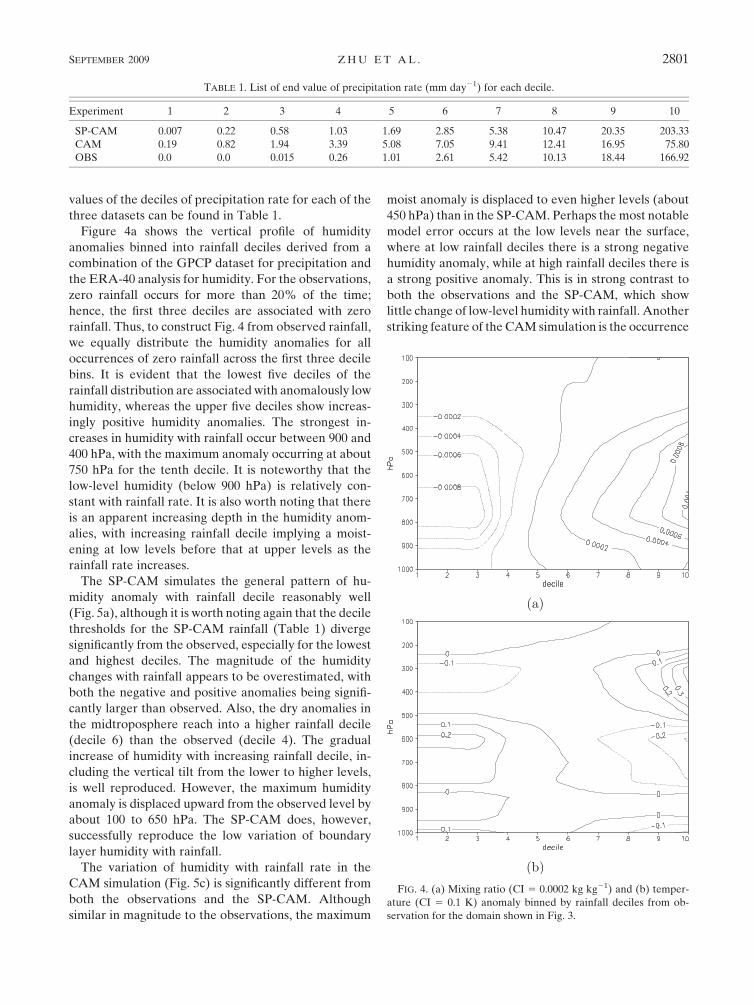
values of the deciles of precipitation rate for each of the

three datasets can be found in Table 1.

Figure 4a shows the vertical profile of humidity

anomalies binned into rainfall deciles derived from a

combination of the GPCP dataset for precipitation and

the ERA-40 analysis for humidity. For the observations,

zero rainfall occurs for more than 20% of the time;

hence, the first three deciles are associated with zero

rainfall. Thus, to construct Fig. 4 from observed rainfall,

we equally distribute the humidity anomalies for all

occurrences of zero rainfall across the first three decile

bins. It is evident that the lowest five deciles of the

rainfall distribution are associated with anomalously low

humidity, whereas the upper five deciles show increas-

ingly positive humidity anomalies. The strongest in-

creases in humidity with rainfall occur between 900 and

400 hPa, with the maximum anomaly occurring at about

750 hPa for the tenth decile. It is noteworthy that the

low-level humidity (below 900 hPa) is relatively con-

stant with rainfall rate. It is also worth noting that there

is an apparent increasing depth in the humidity anom-

alies, with increasing rainfall decile implying a moist-

ening at low levels before that at upper levels as the

rainfall rate increases.

The SP-CAM simulates the general pattern of hu-

midity anomaly with rainfall decile reasonably well

(Fig. 5a), although it is worth noting again that the decile

thresholds for the SP-CAM rainfall (Table 1) diverge

significantly from the observed, especially for the lowest

and highest deciles. The magnitude of the humidity

changes with rainfall appears to be overestimated, with

both the negative and positive anomalies being signifi-

cantly larger than observed. Also, the dry anomalies in

the midtroposphere reach into a higher rainfall decile

(decile 6) than the observed (decile 4). The gradual

increase of humidity with increasing rainfall decile, in-

cluding the vertical tilt from the lower to higher levels,

is well reproduced. However, the maximum humidity

anomaly is displaced upward from the observed level by

about 100 to 650 hPa. The SP-CAM does, however,

successfully reproduce the low variation of boundary

layer humidity with rainfall.

The variation of humidity with rainfall rate in the

CAM simulation (Fig. 5c) is significantly different from

both the observations and the SP-CAM. Although

similar in magnitude to the observations, the maximum

moist anomaly is displaced to even higher levels (about

450 hPa) than in the SP-CAM. Perhaps the most notable

model error occurs at the low levels near the surface,

where at low rainfall deciles there is a strong negative

humidity anomaly, while at high rainfall deciles there is

a strong positive anomaly. This is in strong contrast to

both the observations and the SP-CAM, which show

little change of low-level humidity with rainfall. Another

striking feature of the CAM simulation is the occurrence

TABLE 1. List of end value of precipitation rate (mm day21) for each decile.

Experiment 1 2 3 4 5 6 7 8 9 10

SP-CAM 0.007 0.22 0.58 1.03 1.69 2.85 5.38 10.47 20.35 203.33

CAM 0.19 0.82 1.94 3.39 5.08 7.05 9.41 12.41 16.95 75.80

OBS 0.0 0.0 0.015 0.26 1.01 2.61 5.42 10.13 18.44 166.92

FIG. 4. (a) Mixing ratio (CI 5 0.0002 kg kg21) and (b) temper-

ature (CI 5 0.1 K) anomaly binned by rainfall deciles from ob-

servation for the domain shown in Fig. 3.


of positive (negative) humidity anomalies at around

900 hPa for below (above) median rainfall. For rainfall

deciles above the median rainfall, dry anomalies in the

low troposphere separate the moist anomalies between

the surface and middle troposphere, which is a behavior

different from that seen in observations and SP-CAM.

Overall, the CAM only poorly represents the observed

relationship between rainfall and tropospheric humidity

anomaly.

d. Relationship between precipitation and verticalprofile of temperature

The different treatments of convection in each simu-

lation not only have different effects on the moisture

distribution, but they also influence the vertical distri-

bution of temperature. As with the moisture anomalies,

the temperature anomalies are binned by deciles of

rainfall rate for the observations (Fig. 4b) and the sim-

ulations (Figs. 5b,d). As expected, the temperature

anomalies are small (about 0.28C), reflecting the rela-

tively homogeneous temperature distribution in the

tropics. Nevertheless, several interesting anomaly pat-

terns do occur. At low rainfall rates the observations

show a complicated vertical structure, with weak posi-

tive anomalies in the boundary layer underneath weak

negative anomalies in the lower troposphere and stron-

ger positive anomalies in the midtroposphere with

weak negative anomalies in the upper troposphere. The

stronger midlevel positive anomalies are consistent with

subsiding motion in the midtroposphere, whereas the

cold anomalies above the boundary layer are likely

associated with shallow convection, which cools and

moistens the low levels of the atmosphere near the top

of the cloud layer (Nitta and Esbensen 1974), and those

in the upper troposphere might be associated with a

lack of high-level cloud. Active precipitation (deciles

greater than 5) is associated with strong positive anom-

alies above 500 hPa and with cold anomalies between

800–500 hPa and near the surface. The magnitude of

these anomalies increases with rainfall amount. Impor-

tantly, the shape of the temperature anomaly patterns

for high-rainfall deciles (greater than 5) is consistent

FIG. 5. (a),(c) Mixing ratio anomaly (CI 5 0.0002 kg kg21) and (b),(d) temperature anomaly (CI 5 0.1 K), binned by

rainfall deciles for (a),(b) SP-CAM and (c),(d) CAM.


with a heating–cooling couplet associated with strati-

form precipitation within deep convective systems (e.g.,

Houze 1977) and with numerous other composites of

observed tropical convective systems of various scales

(e.g., Wheeler et al. 2000, their Fig. 7; Haertel and

Kiladis 2004).

The models simulate the observed temperature anom-

alies with mixed success. For the lower deciles of pre-

cipitation (deciles less than 4), the SP-CAM (Fig. 5b)

captures the warm–cold–warm–cold profile in the ver-

tical, while the CAM displays this profile for deciles 3–5.

More interesting, though, are the very strong differences

in model behavior for the upper precipitation deciles.

The SP-CAM reproduces the upper tropospheric warm–

lower tropospheric cold anomaly couplet well, although

it exists only at the highest two deciles, whereas the

observations show its onset around decile 7. The near-

surface cold anomaly is overestimated, indicating a per-

haps too vigorous evaporation of rainfall, which may

simply be due to the overestimation of rainfall rate at the

high deciles (see Table 1). However, SP-CAM still has

some success in representing the vertical structure of the

temperature anomaly, which we hypothesize to be as-

sociated with the presence of stratiform precipitation

processes for the higher rainfall deciles, indicating that

the SP-CAM is able to simulate such processes.

The temperature anomaly structure at high rainfall in

the CAM (Fig. 5d) does not resemble the observed

structure. It is characterized by warm anomalies in both

the upper and lower troposphere, with a very pro-

nounced negative anomaly near 600 hPa and a weaker

cold anomaly near the surface. This anomaly structure

resembles a convective heating profile (warm in the

upper and lower troposphere), interrupted by strong

cooling due to melting of precipitation in the mid-

troposphere. Because the vertical structure of temper-

ature anomaly associated with precipitating convective

systems has a profound influence on the interaction with

the tropical circulation, it is intriguing to note that the

model whose temperature anomaly resembles that of

systems with a significant stratiform component simu-

lates a robust MJO, while the model without such

structure does not.

e. Latent heat flux associated with deep convection

Raymond et al. (2003) studied the convective forcing

in the intertropical convergence zone (ITCZ) of the east

Pacific. They used observations made during the East

Pacific Investigation of Climate year 2001 process study

(EPIC2001) project in the late summer and early fall of

2001 to investigate those factors important to the initi-

ation of deep oceanic convection in the ITCZ. They

found that developing deep convection occurs prefer-

entially in locations with a deep layer that is condition-

ally unstable and is primarily generated and maintained

by surface fluxes of heat and moisture (primarily latent

heat flux). For an approximately 400-km-square region

of the ITCZ, Raymond et al. (2003) observed a crude

balance between the surface flux of moisture and heat

(primarily latent heat) and the drying/cooling tendency

induced by downdrafts (i.e., the boundary layer quasi-

equilibrium hypothesis; Raymond 1995); hence, a strong

correlation was observed between the surface fluxes of

heat and moisture and deep convection.

To study the relationship between latent heat flux and

convection, composites of precipitation anomalies and

latent heat flux anomalies for all occurrences of anom-

alous rainfall greater than 9.65 mm day21 are created.

Note that the rainfall anomaly threshold is somewhat

arbitrary, but is about one standard deviation of rainfall

anomalies for observations (the standard deviation is

calculated over the ocean grid points in the domain

128S–128N, 608–1808E and is about 10.87 mm day21 for

the SP-CAM and 6.5 mm day21 for the CAM). The re-

sults are not sensitive to any threshold greater than the

one chosen here.

Figure 6 shows the evolution of the latent heat flux

anomaly and precipitation anomaly (which is calculated

using the same method as mixing ratio and temperature

anomaly in Figs. 4 and 5) in relation to the strong rainfall

events (rainfall anomaly greater than 9.65 mm day21).

In the observations, the latent heat flux anomaly is seen

to begin to increase about 7 days before peak rainfall

and its peak is coincident with peak rainfall at day 0. The

latent heat flux anomaly then decreases rapidly after

peak rainfall, with the increase and decrease about day 0

being fairly symmetric.

For the SP-CAM simulation, the latent heat flux be-

gins to increase about 5 days before maximum rainfall,

peaks about 1 day after maximum rainfall, and begins to

decline rapidly after day 12. The behavior of the latent

heat flux in the SP-CAM is clearly more realistic but

it displays a distinct 1–2-day lag relative to maxi-

mum rainfall. This behavior is reminiscent of a typical

observed MJO event, with an increase in latent heat

flux lagging the rainfall maximum by a few days (e.g.,

Hendon and Glick 1997). The observed lag of latent heat

flux with respect to rainfall for the MJO is associated

with the occurrence of maximum surface westerly winds

that trail maximum convection by about 1 week (Hendon

and Glick 1997). The occurrence of a phase lag in the

SP-CAM using unfiltered daily data and the absence of

such a lag in the latent heat flux anomaly in the unfil-

tered observations suggests that in the SP-CAM the lag

likely stems from too much of the rainfall variability

being driven by the overly strong MJO (cf. Fig. 2).


In contrast with the observation and SP-CAM, the

latent heat flux in the CAM simulation peaks 2.5 days

before the rainfall maximum and dramatically plunges

at day 0. Precipitation in the CAM is positively corre-

lated with the boundary layer moisture (Fig. 5), and the

strong increase in boundary humidity appears to act to

decrease the surface latent heat flux at the time of

maximum rainfall. The behavior of the latent heat flux

in the CAM is clearly unrealistic, and from the per-

spective of boundary layer quasi-equilibrium (Raymond

1995), the behavior of the latent heat flux in the CAM

would appear to act as a throttle for development of

organized deep convection. The result in the CAM

(minimum latent heat flux at time of peak rainfall) indi-

cates that some of the fundamental assumptions about the

representation of convection in the CAM are flawed.

4. MJO-related convection features

We have so far focused on the behavior of daily av-

eraged tropical oceanic rainfall and the associated var-

iations of humidity, temperature, and surface fluxes on a

grid of roughly 250 km. We now will attempt to relate

this daily-mean gridpoint behavior to the simulation of

the MJO, which of course displays strong spatial and

temporal coherence. To isolate rainfall events that are

related to the MJO, we filter precipitation at each model

and observed grid point to eastward-propagating dis-

turbances for zonal wavenumbers 1–5 with period 30–90

days (e.g., Wheeler and Kiladis 1999). Similar to Benedict

and Randall (2007), MJO-filtered precipitation at each

grid point is chosen as the variable on which MJO events

are based. To explore connections between atmospheric

dynamics and convection during the evolution of the

MJO, we composite a variety of fields relative to the

MJO-filtered precipitation (defined as MJO-prec) at

each ocean grid point in the domain of 128S–128N,

608–1808E. At each grid point, we define an MJO event

as an occurrence of MJO-prec that exceeds 2.5 standard

deviations (the standard deviation is equal to about

4.5 mm day21 for SP-CAM and 2.1 mm day21 for the

CAM). Lag and lead composites of anomaly fields are

formed relative to the time of maximum MJO-prec that

exceeds 2.5 standard deviations at each ocean grid point.

In this fashion, we build up a one-dimensional (height)

lead–lag composite of the evolution of the MJO. We

mainly compare the model simulations to what was

observed in Benedict and Randall (2007).

The mixing ratio composite for the MJO is shown in

Fig. 7a for SP-CAM. Humidity begins to increase above

the boundary layer about 15 days before the peak rain-

fall and then increases over an increasingly deep layer,

with the maximum value occurring in the midtropo-

sphere at lag 0 (when MJO-prec peaks). Little variation

of boundary layer moisture is seen. This progressive

moistening of the low to midtroposphere is consistent

with a similar development of rising motion (Fig. 7b).

About 10 days after peak precipitation, drying is first

accomplished in the lower troposphere and then ex-

pands vertically upward with time. These features of

moistening and drying are similar to the findings of

Benedict and Randall (2007), who studied the observed

characteristics of the MJO relative to maximum rainfall.

They found that the time for the discharge of moisture is

about half of that for recharge. Drying in SP-CAM

happens rather later, around day 8, and returns to the

anomalously dry state by day 13, and the drying rate

after the rainfall maximum is about 2/3 of that for the

moistening rate before the rainfall maximum. The lag

of upper tropospheric humidity relative to that in the

FIG. 6. (a) Daily mean precipitation anomaly (mm day21) and (b) daily mean latent heat flux anomaly (W m22)

composited by the occurrence of daily mean precipitation anomaly greater than 9.65 mm day21 for observation,

SP-CAM, and CAM for the domain shown in Fig. 3.


lower troposphere is surprisingly subtle here in SP-CAM

(about 2 days) relative to observations (about 7 days)

(Benedict and Randall 2007), possibly because for

SP-CAM, 4-km resolution might not be able to resolve

shallow convection sufficiently well to produce an ear-

lier moistening of the lower troposphere (as in the ob-

served) before the maximum precipitation occurs. This

also indicates that in SP-CAM premoistening of shallow

convection may not be a critical factor for the strong

MJO, which has been emphasized as an important fea-

ture in observed MJO in Benedict and Randall (2007).

Figure 7c shows the temperature anomaly relative to

the MJO-prec. Between days 218 and 210, there is a

negative temperature anomaly in the lower tropo-

sphere, which is consistent with a steadily increasing

moisture anomaly possibly associated with shallow con-

vection, as shown in Figs. 7a,b. With time, the conden-

sation heat release from deep convection likely offsets

the adiabatic cooling of ascending motion, and the tem-

perature anomaly becomes positive and reaches into the

middle and upper troposphere at day 0. At the time of

maximum precipitation, the warm anomaly reaches 0.48

at the level of 300 hPa. Meanwhile, cold anomalies occur

in the lower troposphere between days 215 and 12.

Similar to the precipitation decile compositing in Fig. 5,

the temperature anomaly profile at day 0 is consistent

with top-heavy diabatic heating as a result of stratiform

precipitation areas within deep convective systems.

The zonal wind composite (Fig. 7d) indicates that MJO

convection is associated with a deep baroclinic distur-

bance with a transition from surface easterly to westerly

between days 25 and 0. The transition from easterly to

westerly anomalies in Fig. 7d starts near the surface and

the maximum westerlies occur at 800 hPa at day 8. The

baroclinic nature of the zonal wind anomaly is consistent

with the zonal wind being driven by the deep diabatic

heating associated with latent heat release (e.g., Gill 1980).

We also applied the MJO filtering and compositing to

the CAM simulations. We recall that there is no signal of

the MJO in the CAM simulation (cf. Fig. 2). Hence, the

FIG. 7. Daily anomalies of (a) mixing ratio (CI 5 0.0002 kg kg21), (b) vertical velocity (CI 5 0.01 Pa s21),

(c) temperature (CI 5 0.1 K), and (d) zonal wind (CI 5 1 m s21) composited relative to MJO-prec greater than

2.5 times std dev for SP-CAM for the domain shown in Fig. 3.


filtering to MJO wavenumbers and frequencies essen-

tially reveals the behavior of randomly occurring large-

scale rainfall events. Nonetheless, the composites based

on MJO filtered data are of interest because they reflect

the evolution of large-scale convection in the CAM even

though convection in the CAM does not have a pro-

pensity to propagate eastward.

Figure 8 shows composites relative to the MJO-prec

for the CAM (recall that the 2.5 standard deviation

threshold is 2.1 mm day21 as compared to 4.5 mm day21

for the SP-CAM). The composite vertical velocity

anomaly (Fig. 8b) has an amplitude about half that

in SP-CAM and it peaks higher in the troposphere.

The weaker anomalies in vertical motion (and all

other composited variables) are likely due to weaker

convection in CAM model. Consistent with the vertical

velocity field, the mixing ratio anomaly (Fig. 8a) has a

moist anomaly maximum at 550 hPa when the precip-

itation reaches a maximum. The moisture anomaly in

Fig. 8a is about 3 times smaller compared to the value

in SP-CAM. The temperature anomaly (Fig. 8c) has

positive centers in the upper troposphere (about 300 hPa)

and lower troposphere and a strong negative center near

600 hPa, which is similar to the profile for the highest

rainfall decile (Fig. 5d). The lack of any structure in-

dicative of a stratiform heating profile appears to be the

main factor that accounts for the difference in the tem-

perature profile from SP-CAM.

The composite zonal wind anomaly for the CAM is

displayed in Fig. 8d. Easterly winds are dominant be-

tween days 215 and 5 in the low to midtroposphere,

reaching their maximum strength at about 900 hPa at

day 25. With the same contour interval as SP-CAM,

westerly winds are weak and mainly occur at day 5 in the

lower troposphere. However, the baroclinic structure of

the zonal wind seen in SP-CAM is hardly evident, in-

dicating that the zonal wind anomaly is decoupled from

the convective heating source.

Figure 9 shows the MJO-filtered latent heat flux

anomaly. Unlike in Fig. 6 where the compositing was

FIG. 8. As in Fig. 7, but for CAM.


based on any strong rainfall event using unfiltered data,

the observations for the MJO-filtered case show a latent

heat flux maximum at about day 17 (cf. Hendon and

Glick 1997). This lag is well reproduced by the SP-CAM,

even though the amplitude of the anomaly is not. The

CAM shows a reduction in latent heat flux after day 0, but

care must be taken when interpreting this because of the

use of filtering as applied to the CAM that has no MJO.

We now attempt to relate the evolution of the struc-

ture of the anomalies of moisture, temperature, and

vertical velocity associated with the MJO to that in-

ferred from the daily behavior based on the unfiltered

analyses in sections 3c and 3d. For instance, in both

simulations, the vertical profiles of temperature, hu-

midity, and vertical velocity at the time of maximum

MJO rainfall appear to be consistent with the profiles

developed using unfiltered data associated with rainfall

rates in the upper deciles. To confirm this inference, we

compute composites of the occurrence of each unfiltered

rainfall decile when MJO-prec at each gridpoint exceeds

2.5 standard deviations. That is, at each grid point when

the MJO-prec exceeds 2.5 standard deviations, we

accumulate the occurrence of the actual unfiltered daily

rainfall rate in each decile. Then, we combine adjoining

decile thresholds to form quintiles to compact and

smooth the results. We form the accumulation at lags

from 230 days to 130 days, thereby developing a

composite of the rate of occurrence of each rainfall

quintile for the evolution of the MJO.

Figure 10a shows that for SP-CAM the rate of

occurrence of the highest rainfall quintile peaks at about

50% (up from a baseline value of 20%) at day 0 (the

time of maximum MJO-prec), whereas the lowest three

quintiles at day 0 are at a weak minimum (10%, about

half of the baseline rate). Interestingly, the rate of

occurrence of the fourth quintile peaks at about day 210

and then declines gradually through day 110. At day

120, the fifth quintile of precipitation reduces to the

minimum and yields its dominant role to first quintile

precipitation, indicating that in the dry stage of the

MJO, the weakest precipitation quintile occurs most.

Obviously, for SP-CAM, peak MJO-prec (day 0) is

dominated by cases in which the precipitation rate is in

the fifth quintile and the evolution of the temperature,

humidity, and vertical velocity through the life cycle of

the MJO (Fig. 7) can thus be inferred from the associ-

ated profiles for each rainfall quintile (Fig. 5): the evo-

lution of the MJO in the SP-CAM is associated with a

slow buildup of deepening convection that culminates at

day 0 with stratiform-dominated profiles of humidity,

temperature, and vertical velocity.

The associated MJO-filtered composite for the CAM

has some marked difference (Fig. 10b). At the time of

maximum filtered rainfall (day 0), the rainfall rates are

dominated by the highest quintile (with a peak value of

45%), but there is no indication of a preceding shift

from the lower to the fourth quintile prior to day 0.

The evolution of the profiles of temperature, humidity,

and vertical velocity for the MJO-filtered composites

from the CAM are thus consistent with a strong switch

to the highest quintile rainfall rates at day 0, and no

evolution through the lower quintiles occurs in the lead-

up to peak filtered precipitation. Furthermore, in the

dry stage, the first quintile precipitation fails to domi-

nate at day 120, when the fifth quintile precipitation is

the minimum.

Observations (Fig. 10c) shows a similar evolution of

the quintile occurrences to those in SP-CAM, with peak

MJO rainfall being dominated by the fifth quintile and a

minimum for the lowest three quintiles at day 0, and a

slight preceding peak for the fourth quintile at day 210.

This evolution of quintile occurrences for observations

is thus consistent with the vertical development of con-

vection in the lead-up to peak MJO rainfall, as well as

with a stratiform rainfall regime dominating at day 0. At

day 120, the weakest rainfall quintile plays a dominant

role in the dry stage.

5. Discussion and conclusions

The behavior of convection and the MJO are inves-

tigated in two versions of the Community Atmospheric

Model (CAM): the standard model with the Zhang

and McFarlane (1995) convection parameterization

scheme, simply called CAM, and a ‘‘multiscale modeling

framework,’’ in which the cumulus parameterization

has been replaced with a cloud-resolving model, called

SP-CAM. Wavenumber–frequency spectrum analysis

FIG. 9. Daily LHFLX anomaly (W m22) composited relative

to MJO-prec greater than 2.5 std dev for SP-CAM, CAM, and

observations for the domain shown in Fig. 3.


shows that there is a strong MJO, with pronounced

spectral peaks in both precipitation and U850 fields, in

the SP-CAM, but the MJO is completely absent in the

CAM simulation. In this study, we compare aspects

of the behavior of convection in the two simulations

with the aim of understanding which aspects of moist

convection are potentially important for simulations

of the MJO.

We conclude that the following features of convection

are likely affecting the difference in MJO simulations in

the two models:

1) In SP-CAM, rainfall exhibits a strongly exponential

increase with increasing column-integrated relative

humidity, albeit with peak rainfall having too moist an

atmosphere as compared to observations. This sensi-

tivity of rainfall to column-integrated humidity is con-

sistent with the strongest convection having the most

humid conditions. In the CAM, it tends to rain at too

low a saturation fraction, and high saturation fraction/

high rainfall rates are not achieved. This indicates that

the CAM model does not require high column hu-

midity to precipitate; at the same time, the buildup

of high column humidity is prevented, presumably

through the early triggering of convection. These find-

ings are consistent with a large number of earlier

studies, in particular Wang and Schlesinger (1999), who

showed that delaying the onset of convection to

moister conditions generally improved the simulation

of the MJO. The SP-CAM appears to have the mech-

anisms for such a delay built into its formulation.

There is, however, more than one possible expla-

nation for the SP-CAM behavior. One interpretation

of the results is that the replacement of the param-

eterized convection with a CRM leads to the correct

simulation of convection in the model and that this

leads to the improved simulation of the MJO. How-

ever, some of our findings indicate that the onset of

convection in the SP-CAM is delayed to too high

saturation fractions. When precipitation finally occurs,

it occurs with too high an intensity and with a strong

stratiform heating component. We speculate that the

FIG. 10. Frequency of occurrence of precipitation in each quintile composited relative to the occurrence of MJO-prec

exceeding 2.5 std dev for (a) SP-CAM, (b) CAM, and (c) observations.


poor resolution of the CRM embedded in each grid

box (4 km) prevents convection from occurring until

the column has become very moist. The poor reso-

lution might also cause too much of the rainfall to

come from stratiform processes. The combination of

the ‘‘delay’’ in convection and the largely stratiform

nature of the resulting precipitation then leads to the

simulation of a much stronger than observed MJO.

With the data available to us, it is difficult to tell which

of those two alternative explanations is more likely;

this will be the subject of further study.

2) In SP-CAM, heavy precipitation is associated with a

positive–negative temperature anomaly couplet dur-

ing heavy rainfall, possibly indicative of the presence

of a stratiform diabatic heating profile. Such diabatic

heating structures have been shown to project onto

slower horizontally propagating wave modes (e.g.,

Fulton and Schubert 1985 and Mapes 2000). In con-

trast, in the CAM simulation, the temperature profile

is more indicative of a convective-dominated heating

profile that will project onto faster modes.

Lin et al. (2004) found that the observed profile of

heating through the troposphere for the MJO is top

heavy, and stratiform precipitation (heating the up-

per troposphere and cooling the lower troposphere)

contributes more to the intraseasonal rainfall varia-

tions than it does to seasonal-mean rainfall. The role

of the vertical heating profile in setting the strength

and phase speed of intraseasonal oscillations has

been studied in several works. For instance, a

‘‘stratiform instability’’ mechanism has been pro-

posed by Mapes (2000). Yamasaki (1969) found in

numerical modeling studies that some tropical sys-

tems are unstable only if the cumulus heating profile

has a maximum in the upper troposphere. Lin et al.

(2004) argued that a systematic lack of stratiform-

like heating in models could be hypothesized to

contribute to too weak intraseasonal variability and

too fast phase speeds.

Recently, there has been more development of the

theory of stratiform instability (Mapes 2000). A work

by Kuang (2008) found that the effect of midtropo-

sphere humidity on the depth of convection (mois-

ture–stratiform instability) is the main mechanism

for convectively coupled wave development in the

cloud-resolving model. Also, a paper by Raymond

and Fuchs (2009) related the MJO to the completely

distinct moist modes, which are inherently slow

moving. The relationship of the MJO in SP-CAM to

the abovementioned instabilities will be a subject of

our future studies.

3) For observations and the SP-CAM, strong rainfall

events (based on unfiltered gridpoint rainfall) are

associated with increased latent heat flux, whereas

for the CAM, strong rainfall is associated with de-

creased latent heat flux. The latent heat flux in the

SP-CAM is consistent with the notion of boundary

layer quasi-equilibrium, whereby deep convection is

controlled by the moistening and destabilizing effects

of the surface flux of heat and moisture that offsets the

drying and stabilizing tendency induced by unsatu-

rated convective downdrafts (e.g., Raymond et al.

2003). The decrease of latent heat flux at the time of

maximum rainfall in the CAM, which appears to

stem from a spuriously strong dependence of deep

convection on high surface humidity, therefore ap-

pears to act as a throttle for the development of or-

ganized deep convection in the CAM.

In conclusion, this study has developed a number of

innovative diagnostic methods, which, when applied to

two models, appear to show a strong relationship to

those models’ ability to simulate the MJO. The advan-

tages of these new diagnostics over previous techniques

are that (i) they are very simple and (ii) they do not

require the presence of an MJO in the model under in-

vestigation. The disadvantage of the methods proposed

here is that the connection of the model errors revealed

by them to the MJO simulation remains based on cir-

cumstantial evidence only. Applying the techniques to

only two models is obviously insufficient to go beyond

the circumstantial. A natural extension of this work is

therefore to apply the techniques to a wider range of

models. Overall we consider the techniques applied here

to be a promising tool both for identifying the features of

convective behavior that are key to the MJO and for

evaluating their representation in models.

Acknowledgments. We are most grateful to David

Raymond, Matt Wheeler, and Noel Davidson for their

perceptive critiques and constructive suggestion of the

manuscript. We thank Roger Marchand for providing

the data for the two model simulations. We thank the

CMMAP team for their support and in particular David

Randall, Tom Ackerman, Roger Marchand, and Robert

Pincus for discussions on the evaluation of the SP-CAM

model. We thank Zhiming Kuang and an anonymous

reviewer for their constructive review comments on the

manuscript.

REFERENCES

Adler, R. F., and Coauthors, 2003: The version-2 Global Precipi-

tation Climatology Project (GPCP) monthly precipitation

analysis (1979–present). J. Hydrometeor., 4, 1147–1167.

Benedict, J., and D. Randall, 2007: Observed characteristics of the

MJO relative to maximum rainfall. J. Atmos. Sci., 64, 2332–2354.


Bessafi, M., and M. C. Wheeler, 2006: Modulation of South Indian

Ocean tropical cyclones by the Madden–Julian oscillation and

convectively coupled equatorial waves. Mon. Wea. Rev., 134,

638–655.

Bretherton, C., M. E. Peters, and L. Back, 2004: Relationships

between water vapor path and precipitation over the tropical

oceans. J. Climate, 17, 1517–1528.

Collins, W. D., and Coauthors, 2004: Description of the NCAR

Community Atmosphere Model (CAM 3.0). NCAR Tech.

Rep. NCAR/TN-4641STR, 210 pp.

DeMott, C., D. Randall, and M. Khairoutdinov, 2007: Convective

precipitation variability as a tool for general circulation model

analysis. J. Climate, 20, 91–112.

Fulton, S., and W. Schubert, 1985: Vertical normal mode trans-

forms: Theory and application. Mon. Wea. Rev., 113, 647–658.

Gill, A. E., 1980: Some simple solutions for heat-induced tropical

circulation. Quart. J. Roy. Meteor. Soc., 106, 447–462.

Goswami, B. N., 2005: South Asian monsoon. Intraseasonal Vari-

ability in the Atmosphere–Ocean Climate System, W. K. M.

Lau and D. E. Waliser, Eds., Springer Praxis, 19–61.

Grabowski, W. W., 2001: Coupling cloud processes with the large-

scale dynamics using the Cloud-Resolving Convection Param-

eterization (CRCP). J. Atmos. Sci., 58, 978–997.

Haertel, P. T., and G. N. Kiladis, 2004: Dynamics of 2-day equa-

torial waves. J. Atmos. Sci., 61, 2707–2721.

Hayashi, Y., and A. Sumi, 1986: The 30–40-day oscillations simu-

lated in an ‘‘aquaplanet’’ model. J. Meteor. Soc. Japan, 64,

451–466.

Hendon, H. H., and B. Liebmann, 1990: Composite study of onset

of the Australian summer monsoon. J. Atmos. Sci., 47, 2227–

2240.

——, and J. Glick, 1997: Intraseasonal air–sea interaction in the

tropical Indian and West Pacific Oceans. J. Climate, 10, 647–661.

——, M. C. Wheeler, and C. Zhang, 2007: Seasonal dependence of

the MJO–ENSO relationship. J. Climate, 20, 531–543.

Houze, R. A., Jr., 1977: Structure and dynamics of a tropical squall-

line system. Mon. Wea. Rev., 105, 1540–1567.

Kessler, W. S., M. J. McPhaden, and K. M. Weickmann, 1995:

Forcing of intraseasonal Kelvin waves in the equatorial

Pacific. J. Geophys. Res., 100, 10 613–10 631.

Khairoutdinov, M., and D. Randall, 2001: A cloud resolving model

as a cloud parameterization in the NCAR Community Cli-

mate System Model: Preliminary results. Geophys. Res. Lett.,

28, 3617–3620.

——, ——, and C. DeMott, 2005: Simulations of the atmospheric

general circulation using a cloud-resolving model as a super-

parameterization of physical processes. J. Atmos. Sci., 62,

2136–2154.

Kuang, Z., 2008: A moisture-stratiform instability for convectively

coupled waves. J. Atmos. Sci., 65, 834–854.

Lau, N.-C., I. M. Held, and J. D. Neelin, 1988: The Madden–Julian

oscillation in an idealized general circulation model. J. Atmos.

Sci., 45, 3810–3831.

Liebmann, B., H. Hendon, and J. Glick, 1994: The relationship

between tropical cyclones of the western Pacific and Indian

Oceans and the Madden–Julian oscillation. J. Meteor. Soc.

Japan, 72, 401–412.

Lin, J., B. Mapes, M. Zhang, and M. Newman, 2004: Stratiform

precipitation, vertical heating profiles, and the Madden–Julian

oscillation. J. Atmos. Sci., 61, 296–309.

——, and Coauthors, 2006: Tropical intraseasonal variability in

14 IPCC AR4 climate models. Part I: Convective signals.

J. Climate, 19, 2665–2690.

Madden, R. A., and P. R. Julian, 1994: Observations of the 40–50-

day tropical oscillation—A review. Mon. Wea. Rev., 122,

814–837.

Maloney, E., and D. Hartmann, 2001: The sensitivity of intra-

seasonal variability in NCAR CCM3 to changes in convective

parameterization. J. Climate, 14, 2015–2034.

Mapes, B., 2000: Convective inhibition, subgrid-scale triggering

energy, and stratiform instability in a toy tropical wave model.

J. Atmos. Sci., 57, 1515–1535.

Marchand, R. T., J. Haynes, G. Mace, T. Ackerman, and

G. Stephens, 2009: A comparison of simulated cloud radar

output from the multiscale modeling framework global cli-

mate model with CloudSat cloud radar observations. J. Geo-

phys. Res., 114, D00A20, doi:10.1029/2008JD009790.

McPhaden, M. J., 2008: Evolution of the 2006–2007 El Nino: The

role of intraseasonal to interannual time scale dynamics. Adv.

Geosci., 14, 219–230.

Nitta, T., and S. K. Esbensen, 1974: Heat and moisture budget

analyses using BOMEX data. Mon. Wea. Rev., 102, 17–28.

Raymond, D. J., 1995: Regulation of moist convection over the

West Pacific warm pool. J. Atmos. Sci., 52, 3945–3959.

——, 2007: Testing a cumulus parametrization with a cumulus

ensemble model in weak-temperature-gradient mode. Quart.

J. Roy. Meteor. Soc., 133, 1073–1085.

——, and Z. Fuchs, 2009: Moisture modes and the Madden–Julian

oscillation. J. Climate, 22, 3031–3046.

——, G. B. Raga, C. S. Bretherton, J. Molinari, C. Lopez-Carrillo,

and Z. Fuchs, 2003: Convective forcing in the intertropical

convergence zone of the eastern Pacific. J. Atmos. Sci., 60,

2064–2082.

Salby, M. L., and H. H. Hendon, 1994: Intraseasonal behavior of

winds, temperature, and motion in the tropics. J. Atmos. Sci.,

51, 2207–2224.

Sherwood, S., 1999: Convective precursors and predictability in

the tropical western Pacific. Mon. Wea. Rev., 127, 2977–

2991.

Slingo, J. M., and Coauthors, 1996: Intraseasonal oscillations in

15 atmospheric general circulation models: Results from an

AMIP diagnostic subproject. Climate Dyn., 12, 325–357.

Tokioka, T., K. Yamazaki, A. Kitoh, and T. Ose, 1988: The equa-

torial 30–60-day oscillation and the Arakawa–Schubert pen-

etrative cumulus parameterization. J. Meteor. Soc. Japan, 66,

883–901.

Uppala, S. M., and Coauthors, 2005: The ERA-40 re-analysis.

Quart. J. Roy. Meteor. Soc., 131, 2961–3012.

Waliser, D. E., K. M. Lau, W. Stern, and C. Jones, 2003: Potential

predictability of the Madden–Julian oscillation. Bull. Amer.

Meteor. Soc., 84, 33–50.

Wang, W., and M. E. Schlesinger, 1999: The dependence on con-

vective parameterization of the tropical intraseasonal oscilla-

tion simulated by the UIUC 11-layer atmospheric GCM.

J. Climate, 12, 1423–1457.

Weickmann, K. M., G. R. Lussky, and J. E. Kutzbach, 1985: In-

traseasonal (30–60 day) fluctuations of outgoing longwave

radiation and 250-mb streamfunction during northern winter.

Mon. Wea. Rev., 113, 941–961.

Wheeler, M., and G. Kiladis, 1999: Convectively coupled equatorial

waves: Analysis of clouds and temperature in the wavenumber–

frequency domain. J. Atmos. Sci., 56, 374–399.

——, and J. L. McBride, 2005: Australian–Indonesian monsoon.

Intraseasonal Variability in the Atmosphere–Ocean Climate

System, W. K. M. Lau and D. E. Waliser, Eds., Springer Praxis,

125–173.


——, G. Kiladis, and P. Webster, 2000: Large-scale dynamical

fields associated with convectively coupled equatorial waves.

J. Atmos. Sci., 57, 613–640.

Yamasaki, M., 1969: Large-scale disturbances in the conditionally

unstable atmosphere in low latitudes. Pap. Meteor. Geophys.,

20, 289–336.

Yasunari, T., 1979: Cloudiness fluctuations associated with the

Northern Hemisphere summer monsoon. J. Meteor. Soc. Japan,

57, 227–242.

Yu, L., X. Jin, and R. A. Weller, 2008: Multidecade global flux

datasets from the Objectively Analyzed Air–Sea Fluxes

(OAFlux) Project: Latent and sensible heat fluxes, ocean

evaporation, and related surface meteorological variables.

Woods Hole Oceanographic Institution OAFlux Project

Tech. Rep. OA-2008–01, 64 pp.

Zhang, C., and Coauthors, 2006: Simulations of the Madden–Julian

oscillation in four pairs of coupled and uncoupled global

models. Climate Dyn., 27, 573–592.

Zhang, G. J., and N. A. McFarlane, 1995: Sensitivity of climate

simulations to the parameterization of cumulus convection

in the Canadian Climate Centre general circulation model.

Atmos.–Ocean, 33, 407–446.


convection in a parameterized and superparameterized model

Documents