adaptive and variable structure control of a smart
TRANSCRIPT

UNLV Retrospective Theses & Dissertations
1-1-2005
Adaptive and variable structure control of a smart projectile fin by Adaptive and variable structure control of a smart projectile fin by
piezoelectric actuation piezoelectric actuation
Smitha Mani University of Nevada, Las Vegas
Follow this and additional works at: https://digitalscholarship.unlv.edu/rtds
Repository Citation Repository Citation Mani, Smitha, "Adaptive and variable structure control of a smart projectile fin by piezoelectric actuation" (2005). UNLV Retrospective Theses & Dissertations. 1883. http://dx.doi.org/10.25669/1glp-5i2y
This Thesis is protected by copyright and/or related rights. It has been brought to you by Digital Scholarship@UNLV with permission from the rights-holder(s). You are free to use this Thesis in any way that is permitted by the copyright and related rights legislation that applies to your use. For other uses you need to obtain permission from the rights-holder(s) directly, unless additional rights are indicated by a Creative Commons license in the record and/or on the work itself. This Thesis has been accepted for inclusion in UNLV Retrospective Theses & Dissertations by an authorized administrator of Digital Scholarship@UNLV. For more information, please contact [email protected].

ADAPTIVE AND VARIABLE STRUCTURE CONTROL OF A SMART
PROJECTILE PIN BY PIEZOELECTRIC ACTUATION
by
Smitha Mani
Bachelor of Technology Kerala University, Kerala, India
2001
A thesis submitted in partial fulfillment of the requirements for the
Master of Science Degree in Electrical Engineering Department of Electrical and Computer Engineering
Howard R. Hughes College of Engineering
Graduate College University of Nevada, Las Vegas
December 2005
Reproduced with permission of the copyright owner. Further reproduction prohibited without permission.

UMI Number: 1435614
INFORMATION TO USERS
The quality of this reproduction is dependent upon the quality of the copy
submitted. Broken or indistinct print, colored or poor quality illustrations and
photographs, print bleed-through, substandard margins, and improper
alignment can adversely affect reproduction.
In the unlikely event that the author did not send a complete manuscript
and there are missing pages, these will be noted. Also, if unauthorized
copyright material had to be removed, a note will indicate the deletion.
UMIUMI Microform 1435614
Copyright 2006 by ProQuest Information and Learning Company.
All rights reserved. This microform edition is protected against
unauthorized copying under Title 17, United States Code.
ProQuest Information and Learning Company 300 North Zeeb Road
P.O. Box 1346 Ann Arbor, Ml 48106-1346
Reproduced with permission of the copyright owner. Further reproduction prohibited without permission.

UNIE Thesis ApprovalThe Graduate College University of Nevada, Las Vegas
The Thesis prepared by
Sm itha Mani
O ctob er 19 . 20 05
Entitled
'A d a p tiv e and V a r ia b le S tr u c tu r e C o n tr o l Of A Smart
P r o j e c t i l e F in By P i e z o e l e c t r i c A c tu a t io n " _______
is approved in partial fulfillment of the requirements for the degree of
________________ M aster o f S c ie n c e in E l e c t r i c a l E n g in e e r in g
Examination Committee Member
nnatton (xonwnttee Member
Graduate College Faculty Representative
1 /
Examination Committee Chair
Dean o f the Graduate College
11
Reproduced with permission of the copyright owner. Further reproduction prohibited without permission.

ABSTRACT
Adaptive and Variable Structure Control of a Smart Projectile Fin by
Piezoelectric Actuation
by
Smitha Mani
Dr. Sahjendra N. Singh, Examination Committee Chair Professor of Electrical and Computer Engineering
University of Nevada, Las Vegas
The aim of this thesis is to develop efficient control algorithms for the control of
a smart projectile fin in the presence of parameter uncertainties and aerodynamic
disturbance inputs. The fin can be used to maneuver small aerial vehicles by con
trolling its rotation angle. The smart fin considered in this thesis consists of a hollow
rigid body (or canard) within which a flexible cantilever beam with a piezoelectric
active layer is mounted. The beam deforms when voltage is applied to the piezoelec
tric layer. The rotation angle of the fin is controlled by deforming the flexible beam
which is hinged at the tip of the rigid fln. In this thesis, four kinds of fin control sys
tems based on adaptive control and variable structure theory are done. It is assumed
that the fin-beam model parameters and the aerodynamic forces are unknown to the
designer. For this study, a finite dimensional state variable model of the fin-beam
system obtained by a finite element method is used.
I l l
Reproduced with permission of the copyright owner. Further reproduction prohibited without permission.

Firstly, adaptive state feedback and output feedback control laws are designed
for the trajectory control of the fin angle. For the derivation of the control laws,
a stable manifold which is a linear combination of the fin angle tracking error and
its integral and derivative, is chosen. Secondly, an adaptive control system based on
command generator tracker concept is designed using the input, output and reference
command signals. The new control law is simple and unlike the first controller does
not require discontinuous control signal. Next, an output feedback adaptive servoreg-
ulator, exploiting the output feedback passivity property of the system is designed for
trajectory control. Finally, a model reference variable structure adaptive controller
(VS-MRAC) is designed. Unlike the previous adaptive controllers, in this approach,
the adaptation of parameters is not necessary, but the bounds on uncertain functions
are required.
Simulation results using the designed control systems are presented. The results
show that, in the closed-loop system, asymptotic trajectory tracking of the fin angle
is accomplished, in spite of large uncertainties in the system and presence of aerody
namic moment.
IV
Reproduced with permission of the copyright owner. Further reproduction prohibited without permission.

TABLE OF CONTENTS
ABSTRACT ............................................................................................................. iii
LIST OF F IG U R E S ................................................................................................ vii
ACKNOW LEDGMENTS.......................................................................... viii
CHAPTER 1 INTRODUCTION....................................................................... 1Smart F i n ............................................................................................................ 2Types of Smart Materials ................................................................................ 3Adaptive C o n tro l................................................. 3Literature Review................................................................................................ 4Thesis C ontributions.......................................................................................... 6Thesis Outline ................................................................................................... 9
CHAPTER 2 MATHEMATICAL MODEL ..................................................... 10Finite Element Approach.................................................................................... 11Aerodynamic M o m e n t....................................................................................... 14State Variable Representation.......................................................................... 14
CHAPTER 3 STATE FEEDBACK AND OUTPUT FEEDBACK CONTROL 16State Variable Representation.......................................................................... 16Problem D efinition ............................................................................................. 17Adaptive State Feedback C o n tro l.................................................................... 18Adaptive Output Feedback C o n tro l................................................................. 21Simulation R esu lts ........................................ 23
Uncontrolled Dynamics; u=100 V o lts ..................................................... 24Adaptive State Feedback Fin Angle Control: 6 = 5°, 0;=—5° 24Adaptive Output Feedback Fin Angle Control: 9= 5°, 0!=5“ ............. 25
Conclusion............................................................................................................. 25
CHAPTER 4 MODEL REFERENCE ADAPTIVE CO N TRO L................... 29Introductory C o n cep ts ....................................................................................... 29Control Law Design............................................................................................. 32Simulation R e s u l ts ............................................................................................. 39
Adaptive Control: 0 = 5°, a = —5° and + 5 ° ........................................ 40Adaptive Control: 9 = —10°, a = —10° and + 1 0 ° ............................... 41
Conclusion............................................................................................................. 41
Reproduced with permission of the copyright owner. Further reproduction prohibited without permission.

CHAPTER 5 ADAPTIVE SERVOREGULATOR ......................................... 46Adaptive Servocontrol Law................................................................................. 47Simulation R e s u lts ............................................................................................. 51
Adaptive Servo Control: 0 = 5°, a; = — 5" and a = 5 " .................. 52Conclusion............................................................................................................. 52
CHAPTER 6 VARIABLE STRUCTURE ADAPTIVE C O N TR O L 55Fin Model and Control Problem ........................................................................ 56VS-MRAC Law Design....................................................................................... 57Simulation R e s u lts .............................................. 64
Adaptive Control: 0 = 5°, o; = —5", 5 ° .................................................. 65Conclusions.......................................................................................................... 66
CHAPTER 7 CONCLUSION ........................................................................... 69
APPENDIX ...................................................................................................... 72
REFERENCES ...................................................................................................... 74
VITA ......................................................................................................................... 79
V I
Reproduced with permission of the copyright owner. Further reproduction prohibited without permission.

LIST OF FIGURES
1.1 Smart F i n ................................................................................................... 6
2.1 Configuration of Smart F in ....................................................................... 11
3.1 Structure of Adaptive Control System .................................................... 233.2 Uncontrolled dynamics, u = lOOvolts .................................................... 263.3 Adaptive State Feedback Control, 0 = 5°, a = —5 ° .............................. 273.4 Adaptive Output Feedback Control, 6 = a — —5 ° ............................. 28
4.1 Adaptive Control4.2 Adaptive Control4.3 Adaptive Control4.4 Adaptive Control
0 = 5°, a = - 5 ° ........................................................ 42g = a = 5 ° ........................................................... 43e = -10°, a = - 1 0 ° ................................................. 44e = -10°, a = 10 ° .................................................... 45
5.1 Adaptive Servo Control: 0 = 5°, o; = — 5° 535.2 Adaptive Servo Control: 0 = 5°, o; = 5°.................................................. 54
6.1 VSMRAC M o d e l ....................................................................................... 636.2 Variable Structure Control: 0 = 5°, o; = —5° ............................... 676.3 Variable Structure Control: 0 = 5°, o; = 5 ° ........................................... 68
V II
Reproduced with permission of the copyright owner. Further reproduction prohibited without permission.

ACKNOWLEDGMENTS
I would like to express my gratitude to all those who gave me the possibility to
complete this thesis. First and foremost, I offer my sincere gratitude to my advisor.
Dr. Sahjendra N. Singh, who has supported me throughout my MS with his knowledge
and patience. I attribute the success of my thesis to his encouragement and effort.
One simply could not wish for a better or friendlier advisor.
I thank Dr. Woosoon Yim, for his help, advice and guidance during my thesis.
I also want to thank Dr. Venketesan Muthukumar and Dr. Emma Regentova for
serving on my thesis committee.
I would like to dedicate this thesis to my parents, who have always encouraged me
to pursue my dreams. I feel a deep sense of gratitude for them who formed part of
my vision and taught me the good things that really matter in life. This thesis would
not have been accomplished without Bijo, my husband who always gave me warm
encouragement and support in every situation. I owe the deepest thanks to him. I
also thank my friends Shaila and Radhika for supporting me in everyway. Finally, I
thank the staff of the Electrical and Computer Engineering department at UNLV for
providing me with all resources and a nice atmosphere to work in.
Vlll
Reproduced with permission of the copyright owner. Further reproduction prohibited without permission.

CHAPTER 1
INTRODUCTION
Recently, there has been growing interest in using intelligent materials in various
types of structures and structural members. Intelligent materials, when embedded
into the host structures provide wide range of abilities to induce strain or to sense
strain. These abilities make the intelligent materials, a most adequate solution to
various applications such as dynamic actuation, vibration control etc. The use of
surface-mounted or bonded piezoelectric actuators for the shape control of intelligent
structure has gained widespread acceptance recently. Applications can be found in
many areas including the shape control of metallic or composite plates or beams [1,
2]. Applications also involve actuation of various types of aircraft structural members
such as wings, fins, or rotor blade [3, 4, 5, 6]. Advantages of this approach are mainly
due to the integration of the actuators into the structural members itself, thus saving
the space required for servo motors, force transmission devices, or hydraulic systems
[6]. This advantage becomes even more important when small aerial vehicles such as
unmanned aircraft, small missiles, guided munitions, and projectiles, are examined.
Piezoelectric twist actuators used for this application are based on anisotropic strain
ing of the host structure using directionally attached isotropic actuator [3] or using
Reproduced with permission of the copyright owner. Further reproduction prohibited without permission.

piezoelectric fibers integrated into the composite structural members [4]. General for
mulation and solution procedures for an analytical model for a composite laminated
plate with isotropic or anisotropic active layers are derived in Refs. [5, 6].
Traditionally, for the path control of missiles and projectiles, maneuvering forces
and moments are generated by fin angle control using mechanical actuators which are
bulky and slow. For high performance projectiles, there is a need to develop more
efficient actuation mechanisms.
The emergence of small and light-weight actuators associated with smart mate
rials has been triggered recently. Smart materials include electro-rheological fluids,
shape memory alloys and piezoelectric materials. The piezoelectric materials are fea
tured by low power consumption, high power-to-weight ratio and fast response time
compared with other materials. As of now, the piezoelectric materials are normally
employed as sensors as well as actuators for smart structural applications. These
smart structures are primarily employed to control the static and elastodynamic re
sponses of distributed parameter systems operating under variable service conditions.
Smart airfoil - a shape changing wing is the task of current generation aerodynami-
cists. Recently, the development of a smart fln (fin-beam model) has been considered
[7, 8],
1.1 Smart Fin
A smart fin is one which uses smart materials for the shape control of its surface.
Smart materials have unique properties. This model would improve the projectile
Reproduced with permission of the copyright owner. Further reproduction prohibited without permission.

efficiency and performance, since it is aerodynamically perfect. These fins use non-
hydraulic based actuators which can be piezoelectric devices or shape memory alloys.
Hydraulic actuators are heavy and on the contrary smart fins are way too light.
1.2 Types of Smart Materials
There are different types of smart materials available. Some of them are discussed
here. Piezoelectric or electrostrictive material will deform when subjected to an elec
tric charge or a variation in voltage. Electrostrictive materials produce displacements
in same direction where as piezoelectric materials can deform in both directions under
compression and elongation. Magnetostrictive materials undergo induced mechani
cal strain when subjected to a magnetic field. Memory alloys will undergo phase
transformations which will produce shape changes when subjected to a thermal field.
1.3 Adaptive Control
The term adaptive control was introduced in the control literature in the late
1950s and has developed into a broad and vibrant field. Since the early 100s there has
been an exponential growth in adaptive control publications, the earliest publications
originated in aerospace for flight control. The need for adaptive control remains that
of overcoming the difficulty of determining suitable control laws that are satisfactory
over a wide range of operating points. In the 1980s, interest shifted to robust adaptive
control or the adaptive control systems in the presence of perturbations. The main
thrust of the research during the past decade has been in the area of robust adaptive
Reproduced with permission of the copyright owner. Further reproduction prohibited without permission.

control where the aim is to assure the boundedness of all signals in the system even
when external or internal perturbations are present. These perturbations include in
time-varying parameters and structured nonlinearities as well as bounded external
disturbances and the effects of the unmodeled part of the unknown plant.
1.4 Literature Review
Research on smart structure systems associated with the piezoelectric materials
was initially undertaken by Bailey and Hubbard [9]. They proposed simple but effec
tive control algorithms for transient-vibration control, constant amplitude control and
constant gain control. Baz and Poh [10] worked on the vibration control of the smart
structures via a modified independent modal space control by considering the effect
of the bonding layer between the piezoelectric material and the host structure. Tzou
[11] investigated the piezoelectric effect on the vibration control through a modal
shape analysis. Choi [12] improved vibration controllability of the piezofilm actuator
by attenuating undesirable chattering problem in the settling phase.
Numerous researchers have focused on vibration control of the smart structures
associated with the piezoelectric materials. The design of active controllers using
piezoelectric actuators for vibration, force and position control of systems have been
considered by various authors [7, 9, 10, 13, 14]. It is well-known that the piezoelectric
actuators can generate vibration of the flexible structures. In large structures, these
vibrations have long decay times that can lead to fatigue, instability, or other problems
with the operation of the structure. Flexible structures are distributed-parameter
Reproduced with permission of the copyright owner. Further reproduction prohibited without permission.

systems having a theoretically infinite number of vibrational modes. Current design
practice is to model the system with a finite number of modes and to design a control
system using lumped-parameter control theory. Truncating the model may lead to
performance tradeoffs when designing a control system for distributed parameter sys
tems. There exists a wealth of distributed-parameter control theory in the literature.
However, there are very few applications in the literature. The reason may be the
difficulty of using distributed-parameter control theory with spatially discrete sensors
and actuators.
Yim et.ah, [8] proposes a smart projectile fin controller design based on a modeling
error compensation approach in which the lumped uncertainties are estimated using
a high-gain observer. This requires precise measurement of the fin angle for stability
in the closed-loop system. A fuzzy controller has been designed in [15] for the control
of this fin. Of course, for the fuzzy controller design, the designer first has to develop
a number of if-then rules which often are not easy to obtain. Researchers have made
considerable effort to design controllers for the control of flexible structures. Ref.
[16] provides a good review of literature in which readers will find several references.
For flexible structures, controller designs based on feedback linearization, passivity
concepts and adaptive techniques have been attempted [14, 17, 18, 19]. But the
methods based on passivity [20, 21] have advantage over other design techniques since
the passivity approach does not rely on model truncation or higher-order models of
the structure and is independent of the numerical values of the model data.
Reproduced with permission of the copyright owner. Further reproduction prohibited without permission.

Piezoelectric beam actuator
Cross-sectional View of Smart
Fin(AeB)
Before rotation Hinge joint fixed to projectile body
w(L,t)
After rotation
Geometry of cross-sectionai bp A
area of beam *actuator(EOFO
hb
Ep
Hollow fin
-Neutral Axis,D
Figure 1.1: Smart Fin
1.5 Thesis Contributions
This thesis treats the question of adaptively controlling the rotation angle of a
smart fin developed for a subsonic projectile using piezoelectric actuation. Smart
fins are deployed after the projectile reaches the apogee. They are used to guide the
projectile precisely to the target. The schematic of a smart fin investigated as part
of the study is shown in Figure 1.1.
The smart fin considered here has an outer hollow rigid body, within which a
flexible cantilever beam with a piezoelectric active layer is mounted. The rotation
angle of the fin is controlled by deforming the flexible beam which is hinged at the
tip of the rigid fin.
Efficient adaptive control algorithms are developed for the control of rotation an
Reproduced with permission of the copyright owner. Further reproduction prohibited without permission.

gle of a projectile’s fin in the presence of parameter uncertainty and disturbance
inputs. Flexible structures are essentially infinite dimensional systems; however of
ten finite dimensional models by neglecting the higher modes are used for analysis
and design. The models of flexible structures are generally obtained by solving the
eigenvalue problem resulting from finite element methods. However, it is well known
that the resulting fidelity of model parameters degrades drastically for higher modes.
Finite element approach is used to describe the dynamics of the flexible beam with
active layer of piezoelectric actuator. The beam is modeled using a series of finite
elements satisfying Euler-Bernoulli’s theorem. The input signal is the voltage applied
to piezoelectric actuator and the output variable is the rotation angle of the fin.
First, state feedback and output feedback adaptive control systems are derived
for the control of rotation angle of the fin. The fin is controlled by regulating the tip
deflection of the flexible beam which in turn causes the control of the rotation angle
of the fin. A feedback linearizing adaptive control law is designed for the trajectory
control of the fin angle of the flexible beam. For the feedback linearizing control law
design, a stable manifold which is a linear combination of the fin angle tracking error
and its integral and derivative, is chosen. For the purpose of design, it is assumed
that the model parameters are not known. The designed adaptive control systems
forces the trajectory to converge to the chosen manifold. Simulation results show
that in the closed loop system, precise fin angle control is accomplished in spite of
uncertainties in the system parameters, using state as well as output feedback.
Next, based on command generator tracker concept, a model reference adaptive fin
Reproduced with permission of the copyright owner. Further reproduction prohibited without permission.

8
angle controller is designed. The structure of the control system is independent of the
dimension of the flexible fin-beam model. For the design of the control law, a linear
combination of the fin angle and the fin’s angular rate is chosen as the controlled
output variable. In closed-loop system, the controlled output variable tracks the
reference trajectory and the fin angle asymptotically converges to the desired value
and the elastic modes converge to their equilibrium values. Simulation results show
that the fin angle is precisely controlled in spite of uncertainties in the fin-beam
parameters and the aerodynamic moment coefficients.
Next, an adaptive servoregulator is designed for the control of the fin angle and
the rejection of the disturbance inputs. Exploiting the output feedback passivity
property of the system, a direct adaptive control law is derived for the regulation
of the fin angle. Simulation results show that the adaptive servoregulator controller
accomplishes fin angle control.
Finally, a new control system based on the theory of variable structure adaptive
control using only input and output signals are derived. Here only the fin angle
measurement is required for the controller synthesis. Control using the fin angle
is very practical since measurement of flexible modes is not easy. However, it is
assumed that an upper bound on the uncertain functions is given. It is shown that
in the closed-loop system, fin angle tracks given reference trajectory. Unlike other
adaptive controllers developed in literature, controller parameter divergence cannot
occur here since integral type adaptive laws for updating controller are not used in
this design. Simulation results are presented which show good transient response and
Reproduced with permission of the copyright owner. Further reproduction prohibited without permission.

robustness to uncertainty and unmodeled dynamics.
1.6 Thesis Outline
The following is a brief summary of the outline of this thesis report. Chapter 2
introduces mathematical modeling of the projectile fin. Chapter 3 derives the adap
tive state feedback and output feedback control laws. A model reference adaptive
controller is designed in Chapter 4. Chapter 5 describes adaptive servoregulator.
Chapter 6 describes variable structure adaptive controller. Finally, Chapter 7 in
cludes the conclusion of this thesis and suggestions for future work.
Reproduced with permission of the copyright owner. Further reproduction prohibited without permission.

CHAPTER 2
MATHEMATICAL MODEL
This chapter deals with the mathematical modeling of the fin-beam system. The
schematic of the fin-beam model is shown in Figure 2.1. The fiexible beam with a
piezoelectric active layer bonded on the top surface, is hinged at one end to the fin
and the other end is attached rigidly to the projectile body. The fin is free to rotate
about an axis fixed to the projectile body. When the control voltage u(x, t) is applied
to the actuator, the induced strain in the actuator generates the bending moment m
that is expressed as [9]
m = cu{x,t) (2.1)
The constant c can be obtained by considering geometrical and material properties
of the beam and piezoelectric actuator. Considering the cross sectional geometry and
force equilibrium along the axial direction, the constant c can be expressed as [12]
where d^i is the piezoelectric strain constant and Ep and Ft are Young’s modulus
of the piezoelectric actuator and the beam respectively. Other geometric parameters
are shown in the figure.
10
Reproduced with permission of the copyright owner. Further reproduction prohibited without permission.

11
Top view o( Sm art Fin
Rigid in
Hinged connection
Cantilever beam piezoelectricactuator
% E d...-----
Ebh
D..N e u tr a l ax is
Figure 2.1; Configuration of Smart Fin
As shown in Figure 2.1, the fin is free to rotate about the hinge joint fixed to the
projectile body and one end of the beam actuator is fixed to the projectile body and
the other end is connected the fin using another hinge joint fixed to the tail side of
the fin. The fin is considered as rigid and its rotation angle is assumed to be small
and planar.
2.1 Finite Element Approach
Finite element approach is used to describe the dynamics of the flexible beam,
which is considered as composed of finite elements satisfying Euler-Bernoulli’s theo
rem. The beam is divided into n elements with equal length of Li. The displacement
w of any point on the beam element i is described in terms of nodal displacement,
Reproduced with permission of the copyright owner. Further reproduction prohibited without permission.

12
Wi, and slope, (j)i, at node i and % + 1, respectively and is expressed as
w — Nqi (2.3)
where % = {wi, (j)i, and N = (TVi, jVg, N 3 , N 4 ) is the shape function vector
with
Ni = j ^ ( 2 x\ — SxjLi + Li)
N 2 = j^{x fL i — 2x^Lj + XiLi) (2.4)
Ns = ^ ( — + Sx^Li)
N , = - x l L l )
where Xi is the element local coordinate variable defined along the beam neutral axis.
Using Eq. (2.4), the kinetic energy of an element i becomes
î i = ^ / pi'ùP'dxi = ^qfMiQi (2.5)
where M* G piN'^Ndxi) is a mass matrix and pi is a combined density of
the beam and piezoelectric actuator per unit length.
The potential energy of an element i is
1 1 LP'ih^ ‘ = 2 1 + P-6)
where Eili is the product of Youngs modulus of elasticity by the cross-sectional area
moment of inertia for the equivalent beam of an element i. If the piezoelectric actuator
has a uniform geometry and that a uniform voltage is applied along its length, u{x,t)
Reproduced with permission of the copyright owner. Further reproduction prohibited without permission.

13
can be assumed to be function of time only. The potential energy of an element can
be further expressed as,
1 _ 1 1K = + g f ^ d x t ) c u ( t ) + ~ f A t )
where the stiffness matrix K. € becomes
(2.7)
(2.8)
The kinetic energy of the rigid fin is
T, = (2.9)
where J / is the mass moment of inertia of the fin about an axis fixed on the projectile
body and Wn+i is the time derivative of tip deflection Wn+i or w{L,t).
Using the Lagrangian dynamics, the equations of motion for the element i becomes
(2 .10)
where Bi = (0, —1,0, —1)^ which represent two concentrated moments at two nodes
of the element i. For the last element (i = n), the equation of motion including the
mass of the rigid fin becomes
MjiQn T
0 0 0 0
0 0 0 0
0 0 0 0
Qn T KnQn — ^ n ( Cu(t)) (2 11)
The equations derived for each element can be assembled after expansion and matrix
Reproduced with permission of the copyright owner. Further reproduction prohibited without permission.

14
reduction from the boundary conditions of the cantilever beam as follows,
Mq + Kq — Bou{t) (2.12)
where q = (wg, < , . . . , Wn+l, 4>n+l)' E 9? ”, M G Sjj2nx2n % G 3?2nx2n g
are appropriate matrices.
2.2 Aerodynamic Moment
The aerodynamic moment acting on the fin is a complicated function of the angle
of attack of the projectile and the fin rotation angle. The data generated by the
computational fluid dynamics show that the aerodynamic moment can be accurately
modeled as a linear function of the fin angle with a bias term and a reasonable model
can be expressed as
rria = mao{a) + Pa{a) 6 = mao{a) + Pa{a)r'^e*'^q (2.13)
where 6 is the fin angle, a is the angle of attack, Pa{d) is a polynomial in the angle of
attack, a , Pa{0) = Po +Pi(^) + •••■ (A is a positive integer) and e*^ G is a
unit vector whose (2n — l)*/i element is one and rest are zero.
2.3 State Variable Representation
The modified fin-beam model including the aerodynamic moment takes the form
Mq + Kq = B^uit) -f BatUa (2.14)
Reproduced with permission of the copyright owner. Further reproduction prohibited without permission.

15
where Ba = [0, ...0,1,0]^ G Substituting ma from Eq. (2.13) in Eq. (2.14), and
solving the resulting equation
q = - M ^Kmq + M ^Bou{t) + M ^Bamao{a) (2.15)
where = K — Pa{oi)l e*e*^, now includes the cr-dependent term of the aerody
namic moment.
This reduced dynamic model using n elements can be expressed in the state vari
able form using the state vector x = (ç^, g^)^ G as
X =0 InX‘
-M-^Krr,. 0X +
0 .nxl
M-iRou{t) -f
Onxl
M-^Barriaoiot)
Ax -f Bu + Dmao{a) (2.16)
where the matrices A, B and D are defined in Eq. (2.16). Since the interest is in the
control of the fin angle, we associate with the system Eq. (2.13), a controlled output
variable given by
P = 0 (2.17)
where 6 is the fin angle.
Let a smooth and bounded reference fin angle trajectory 6 is given. We are
interested in designing an adaptive control law such that in the closed-loop system
the fin rotation angle asymptotically tracks 6 r and the state variables remain bounded
during maneuver.
Reproduced with permission of the copyright owner. Further reproduction prohibited without permission.

CHAPTER 3
STATE FEEDBACK AND OUTPUT FEEDBACK CONTROL
In this chapter, state feedback and output feedback adaptive control laws are derived
for the trajectory control of the rotation angle of the projectile’s fin. For the purpose
of design, it is assumed that the model parameters are not known. The fin is controlled
by regulating the tip deflection of the flexible beam which in turn causes the control
of the rotation angle of the fin. The input signal is the voltage applied to piezoelectric
actuator and the output variable is chosen to be the rotation angle of the fin.
3.1 State Variable Representation
As derived in Chapter 2., the reduced dynamic model using n elements can be
expressed in the state variable form using the state vector x = {q^, E as
X =0 InX‘
-M-^Krr,. 0
X +OjlXl
M-^Bou{t)
Ojixl
M-^Bamao{a)
= Ax + Bu + Dmaoid) (3.1)
where the matrices A, B and D are defined in Eq. (3.1). The controlled output
variable is given by
3/ = 0 (3.2)
16
Reproduced with permission of the copyright owner. Further reproduction prohibited without permission.

17
where 6 is the fin angle.
3.2 Problem Definition
Let a smooth and bounded reference fin angle trajectory 6 r is given. An adaptive
control law has to be designed such that in the closed-loop system the fin rotation an
gle asymptotically tracks 6 and the state variables remain bounded during maneuver.
For the design of control system, it is assumed that the designer has no knowledge of
the system. It is assumed here that the matrices M~^Bq and M~^Ba are
unknown.
For the derivation of the control laws, a stable manifold which is a linear combi
nation of the fin angle tracking error and its integral and derivative, is chosen. The
designed adaptive control systems force the trajectory to converge to the chosen man
ifold. The manifold is such that the tracking error for any trajectory confined to it
asymptotically tends to zero.
The fin angle is given by
= (3.3)
where w{L, t) denotes the tip deflection of the flexible beam. For a small tip deflection
one can approximate the fin angle as
(3.4)
That is, 0 is proportional to w{L,t). Of course, the proposed design approach is
applicable even if 6 is given by the nonlinear Eq. (3.3).
Reproduced with permission of the copyright owner. Further reproduction prohibited without permission.

18
Differentiating 6 along the solution of Eq. (3.1) gives
6 — CA^x + CABu +CADmao{cx) (3.5)
3.3 Adaptive State Feedback Control
In this section a state variable feedback adaptive control law is derived. For the
purpose of control law derivation, a stable manifold of the form
S — 9 2 u!fi9fi + u> I Odrf Odr (3.6)J o
is chosen, where 9 — 6 — Or is the fin angle tracking error, ( > 0 and a;„ > 0. In
view of [22] one finds that if 8=0 (that is, the trajectory is confined to the manifold
8=0) then 9{t) -4 0, as t > oo, and the fin angle asymptotically tracks the prescribed
trajectory Or- Therefore, it is sufficient to design a control law such that S{t) tends
to zero.
The design is based on the Lyapunov approach [22, 23, 24]. Differentiating S and
using Eq. (3.5) gives
S = CA^X + CABu T CAD i71(iq(Cx) — 9r 2( UJn9 +
= iJ^Xa + bou + g{9,9,t) (3.7)
where u = [{CA‘ f ,C A D ] e bo = CAB e R, Xa = (z^ .l) E and
g {9 ,9, i) = —Or + 2QujnO + uj O
We note that u is an unknown parameter vector. Let z> and p be the estimates of
V and = p. Then the parameter errors are ü = u — ù and p = p — p.
Reproduced with permission of the copyright owner. Further reproduction prohibited without permission.
19
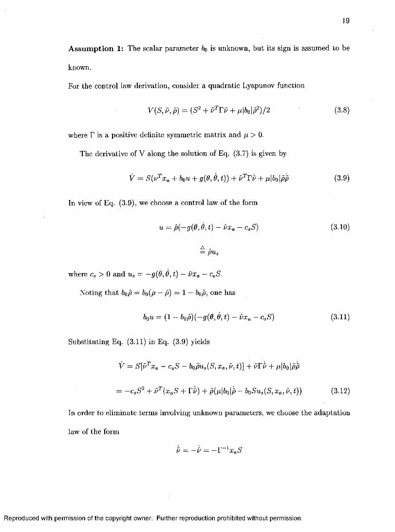
Assumption 1: The scalar parameter bo is unknown, but its sign is assumed to be
known.
For the control law derivation, consider a quadratic Lyapunov function
y(5', P, p) = (g" + P^FP + /i|6o|p')/2 (3.8)
where F is a positive definite symmetric matrix and p > 0.
The derivative of V along the solution of Eq. (3.7) is given by
V = S{i''^Xa + bou + g{6,9,t)) + f/^FP + p|6o|pp (3.9)
In view of Eq. (3.9), we choose a control law of the form
u = p{-g{9,9, t) - ùxa - CsS) (3.10)
A .— P^s
where c, > 0 and Ug = -g{9 ,9, t) - ùXa - CgS.
Noting that boP = bo{p — p) = 1 — bop, one has
bou = (1 - bop){-g{9,9, t) - ùxa - CgS) (3.11)
Substituting Eq. (3.11) in Eq. (3.9) yields
V = S[u^Xa - CgS - bopUg{S,Xa,û,t)] + î>FP + p|6o|pp
= -CgS'^ + v^{xaS + FP) + p(p |6o|p- boSug{S,Xa,i>,t)) (3.12)
In order to eliminate terms involving unknown parameters, we choose the adaptation
law of the form
Û — —Ù — —T~^XaS
Reproduced with permission of the copyright owner. Further reproduction prohibited without permission.

20
p = - p = {sgn{bo))us(S, Xa, P, t )p^^S (3.13)
Substituting Eq. (3.13) in Eq. (3.12) gives
ÿ = -0,5" (3.14)
Since E is a positive definite function of 5, P and p, and V is negative semidefinite,
according to Ref. [22], it follows that S, z>, p are bounded functions (denoted as
Loo[0, oo)) and E(oo) exists. Integrating Eq. (3.14) gives
pooc, / = y(0) - y(oo) < oo (3.15)
J o
which implies that S E I/2[0 , oo) (square integrable function). Also in view of Eq.
(3.7) S E Loo[0, oo) if X is bounded. Then it follows from the Barbalat’s lemma [24,
25], that S{t) —> 0 as t —> oo; which implies that the tracking error 9{t) -4 0 as
t ^ oo. Thus in the closed-loop system, fin angle asymptotically follows the given
reference trajectory 9r{t).
The above arguments for trajectory control are based on the assumption that the
zero dynamics have bounded solution. Zero dynamics describe the residual motion
of the fin when the fin angle is identically zero. The stability of the zero dynamics
depend on the zeros of the transfer function 9{s)/ü{s) = H{s), where the overbar
denotes the Laplace transform and s is the Laplace variable. For the fin model,
computing H{s) one finds that H{s) has purely distinct imaginary zeros. As such,
when the fin angle is controlled to a constant value, the residual elastic modes will
have persistent, but bounded oscillations consisting of sinusoidal signals.
Reproduced with permission of the copyright owner. Further reproduction prohibited without permission.

21
For the synthesis of the control law Eq. (3.10) and the adaptation law Eq. (3.13),
one needs to measure all the state variables. A sufficient number of sensors can
be used to obtain the measurement of x. However it is of interest to synthesize a
controller using only fin angle and its derivative. We can modify the control and
adaptation laws to accomplish this.
3.4 Adaptive Output Feedback Control
In this subsection, synthesis using only output feedback is considered. Of course
one can design an adaptive feedback control laws using traditional adaptive control
techniques [25, 26], however such an attempt is not made here because these adaptive
controllers are quite complicated. Instead here we are interested in designing a control
law which can be easily synthesized.
Let
= uFym + (3.16)
where Xr denotes those variables of Xa which are not measured, w E 9% and =
{9,6,1)^ E is assumed to be available for feedback. We assume that w is an
unknown parameter vector, but is treated as a disturbance input.
For the purpose of design consider a Lyapunov function
W = (S^ + w^riW + p|6o|p^)/2 (3.17)
where Fi > 0 and p > 0. Then its derivative along the solution of Eq. (3.7) is given
by
W = S{u'^ym + bou + g{9,9,t) + vjxr) + w^Fiw + p |6o|pp
Reproduced with permission of the copyright owner. Further reproduction prohibited without permission.

22
< S\üFDm + dFVm + bou + g{9,9, t)] + \S\k* + ùF T iü + p |6o|pp (3.18)
where k* is constant such that k* > \t^^Xr\.
In view of Eq. (3.18), we choose a control law
u = p{-CFym - g - C i S - k*sgn{S))
= (3.19)
and the adaptation rule as
à) = - r ~ Sym
p = S v s S g n { b o ) / p (3.20)
Then substituting Eq.s (3.19) and (3,20) in Eq. (3.18) gives
# < -Cig^
Now using a similar argument, one can show that 0 -4 0, as t —)■ oo, provided that
Xa remains bounded during the maneuver. The results of next section indeed show
that it is the case and by a proper choice of k*, fin angle control with the control
law (Eq. (3.19)) is accomplished. The control law in Eq. (3.19) is discontinuous
and one can use a continuous approximation of the sgn function using a tanh(s)
function. However, in this case some modification in the adaptation law, Eq. (3.20)
(for example cr-modification [25] may be required to avoid the parameter divergence.
The structure of an adaptive control system with state feedback or output feedback
is shown in Figure 3.1.
Reproduced with permission of the copyright owner. Further reproduction prohibited without permission.

23
Xr r
a , â
Controller Fin—Beam System
Figure 3.1: Structure of Adaptive Control System
3.5 Simulation Results
This section presents the simulation results for the smart fin (fin-beam model)
including the state as well as output feedback systems. The mechanical properties of
the simulated model are given in the appendix. Using finite element method (with
n=5 elements), a state-variable representation of the fin-beam model of dimension
of 20 is obtained for simulation. The controller parameters chosen are given in the
appendix. For simplicity, integral feedback is not used in the manifold Eq. (3.6) (i.e,
(jJn=0)- Reference command trajectories are generated by a third order command
generator given by
where 6 * is the desired fin angle. Ci, Ac and Uc are chosen to obtain desirable fin angle
reference trajectories (see the appendix). Here 6 * is taken for an angle of 3°, which
corresponds to the tip deflection of 0.0073m.
Reproduced with permission of the copyright owner. Further reproduction prohibited without permission.

24
3.5.1 Uncontrolled Dynamics: u=100 Volts
For examining the uncontrolled behavior, the fin-beam model Eq. (3.1) without
the adaptive controllers is simulated. The initial condition is set to x{0) = 0 and
a constant voltage u = 100 volts is applied to the system. Selected responses are
shown in Figure 3.2. We observe that each state variable has persistent but bounded
oscillations. The fin angle as well as the deflection variables(w2, ..., wq) oscillate about
nonzero average values in the steady state. Note that we = w{L), the tip deflection
and Wi = 0. It is seen that amplitude of oscillations of Wi monotonically increases
with i as expected. For the chosen applied voltage, the maximum fin angle is less
than 1.75° in the steady state.
3.5.2 Adaptive State Feedback Fin Angle Control: 9= 5°, o;=—5°
First we present the results using the adaptive law Eq. (3.10) with state variable
feedback. The initial values of the parameters chosen are 0(O)=O and p(0)=0.5776.
The actual value of p is 11.5511; therefore, the estimated value of p is l/20th of the
actual value. We have made a worse choice of parameter estimate of 6 in order to
show the robustness of the controller. The selected responses are shown in Figure 3.3.
We observe that the fin angle converges to the desired value (5°) in about 2 seconds.
The deflections at other points on the beam remain bounded during the maneuver
and seem to converge almost to constant values. Apparently, oscillatory components
of the flexible modes as well as the control input are negligible in the steady state.
The control input required is about 600 volts, which is reasonable. The maximum fin
angle tracking error is less that 2 x 10“° degrees, which is quite small.
Reproduced with permission of the copyright owner. Further reproduction prohibited without permission.

25
3.5.3 Adaptive Output Feedback Fin Angle Control: 6 = 5°, o;=5°
Now the adaptive control law, Eq. (3.19) using only the measured signal ym=
(0,9)'^ is synthesized and simulation results are obtained. The initial estimates of
parameters are w(0)=0 and p(0)=(l/20)p. The value of ci is set to 20. This value
has been chosen by observing the simulated responses. The remaining parameters of
Figure 3.3 are retained. Simulated responses are shown in Figure 3.4. We observe that
the controller using output feedback is effective in trajectory tracking and desired fin
angle is smoothly obtained in less than 3 seconds. The deflections at the other points
on the beam also have responses which are some what similar to those of Figure 3.3.
The peak value of the control input remains of the same order and the maximum fin
angle tracking error is 2 x 10“°. It is found that one can obtain faster response using
larger values of k*, however this will require larger input voltage.
3.6 Conclusion
In this chapter control of a smart fin (rigid fin-flexible beam model) of a projec
tile was considered. The flexible beam with a piezoelectric active layer was used for
rotating the fin. A state variable model obtained using the finite element method
was used. State-variable feedback and output feedback adaptive control laws were
developed. In the closed-loop system trajectory tracking of the reference fin angle was
accomplished. Simulation results obtained show that fin angle can be smoothly con
trolled to desirable values by using either of the controllers in spite of large parameter
uncertainties.
Reproduced with permission of the copyright owner. Further reproduction prohibited without permission.

26
1.5
330.5
0.5 1.5Time (sec)
x lO ”'
E
I3
2
1
0
■120 0.5 1 1.5
I5
4
3
2
1
0. 0.5 1 1.50 2Time (sec)
X 10
Time (sec)
20
& 15S 10
.1
§-5 .
0.5 1.5Time (sec)
CL-0.1
0.5 1 1.5T im e ( s e c )
2 4T ip D e fle c tio n (m j ’
Figure 3.2: Uncontrolled dynamics, u = lOOvolts
Reproduced with permission of the copyright owner. Further reproduction prohibited without permission.

27
0.015
0.01
o ^ 0.005
CL
Time (sec) Time (sec)
5oa
gI<DQ
x IO 'X 108
6 oS10
4 i/ic
2
0 - 560 2 4
Time (sec) Time (sec)X 10"
600
T3> 400
g- 200 LU - 2 o>
-2 00
Time (sec) Time (sec)
CL 1.5 ■o 0.01
o 0.005
lÏÏ 0.5 .O:,0.005
- 0.01
Time (sec) Time (sec)
Figure 3.3: Adaptive State Feedback Control, 6 = 5°, a = —5°
Reproduced with permission of the copyright owner. Further reproduction prohibited without permission.

28
0.0156
5
c 0.014
3
0.0052
1 CL0
2Time (sec)
3 410Time (sec)
X 10600
> 400
Q- 200
O)c
œ - 2 . -2 0 04
Time (sec) Time (sec)0.0325
0.025
ro 0.02
% 0.015E 10
o 0.01UJ
0.005
4Time (sec)Time (sec)
X 100.015
M 0.01
LU
g -2> 0 .0 0 5
- 0.01-64
Time (sec)Time (sec)
Figure 3.4: Adaptive Output Feedback Control, 0 = 5°, a = —5°
Reproduced with permission of the copyright owner. Further reproduction prohibited without permission.

CHAPTER 4
MODEL REFERENCE ADAPTIVE CONTROL
In the previous chapter, an adaptive controllers based on inverse feedback lineariza
tion technique were designed. This required synthesis using either the state feedback
or discontinuous output feedback control. For state feedback, one needs to measure
all the state variables. This requires sufficient number of sensors to obtain the mea
surement of states. In output feedback control, the controller was designed using
only the fin angle and its derivative. All the other states which are not measured are
treated as disturbance inputs.
4.1 Introductory Concepts
Based on the command generator tracker concept, a model reference adaptive fin
angle controller is designed in this chapter. For the trajectory control of the fin angle,
a judicious choice of a controlled output variable, which is a linear combination of
the fin angle and fin’s angular rate is chosen. The control law does not depend on
the dimension of the state space of the fin-elastic beam model. This is important
because controller designed based on truncated models of flexible structures may
encounter instability due to control and observer spillover. In the closed-loop system
29
Reproduced with permission of the copyright owner. Further reproduction prohibited without permission.

30
the fin angle asymptotically converges to the target fin angle generated by a command
generator and all the elastic modes converge to their equilibrium values.
The aerodynamic moment affecting the projectile fin can be expressed as (Eq.
(2.13))
rria = niaoio:) + Pa{a) 6 = mao{a) + Pa{a)r^e*'^q (4.1)
where 6 is the fin angle, a is the angle of attack, Pa{&) is a polyomial in the angle of
attack, a, Pa{0) = Po + P i { d ) + ■••• ( t is a poisitive integer) and e*^ e is a
unit vector whose (2n — l)*h element is one and rest are zero.
The modified fin-beam model including the aerodynamic moment takes the form
Mq + Kq = Bou{t) + BaUia (4.2)
where Ba — [0, ...0,1,0]^ e Solving Eq. (4.1) gives
q = -M ^^Kmq + M~^Bou{t) -t- M~^Bamao{a) (4.3)
where Km ~ K — pa{a)L^^e*e*'^.
The eigenvalues of M~^Km are distinct positive real numbers. As such there
exists a similarity transformation matrix V formed by the eigenvectors of the matrix
M^^Km such that
(4.4)
where = diag(nf), % = 1,..., 2n; Qj, i ^ j .
Defining 77 = V~^q, one obtains from Eq. (4.3)
77 = - 0 ^ 7 7 -h y - " M - ^ B o i ^ ( t ) + y - " M - ^ B . 7 M ^ ( a )
Reproduced with permission of the copyright owner. Further reproduction prohibited without permission.

31
= — + Biu(t) + di (4.5)
where Bi = V^^M~^Bo G and c?i = V~^M~^Bamao{a). The modal form Eq.
(4.5) has no damping. However, there is nonzero structural damping for any elastic
body. As such it is common to introduce a dissipation term proportional to the rate
■q. Introducing a damping term of the form 2DQ,, where D = diag{Ci), i = 1, ...,2n,
Q > 0 , one obtains the system
q = —2DQq — fl^q + Biu + d\ (4.6)
The fin angle in new coordinate becomes
9 — L~^e*^q — L~^e*^Vq = Coq
where Q =
It is assumed that the system matrices D, Q, B\ and Co are unknown. Fur
thermore, it is assumed that only the fin angle and the angular rate is measurable.
Consider a first-order reference model of the form
~ -^m^m T Bm'IJ'm (4:.7)
Vm ~ (4.8)
where E 5ft"*, 7/ ^ 6 % and Am is a Hurwitz matrix. We are interested in designing
an adaptive control system such that the fin angle asymptotically tracks the reference
trajectory i/m- Moreover, for synthesis only the measured angle 9 and 9 are to be used.
Reproduced with permission of the copyright owner. Further reproduction prohibited without permission.

32
4.2 Control Law Design
In this section, an adaptive controller will be designed. Defining the state vector
X = G a state variable representation of Eq. (4.5) takes the form
02nx2n I2nx2n
- 2 DQx + 02nxl
u +02nxl
d\
A X + Bu + d (4.9)
where d = [0 ix2n,(^]^ and B — [0ix2n , W e associate with Eq. (4.9), an output
variable
(4.10)
where C is yet to be chosen. In Eq. (4.9), d is treated as a disturbance input. An
ideal system is obtained when the disturbance d is zero. This ideal state equation is
given by
X = A X + Bu (4.11)
with its associated output given in Eq. (4.10). For the design of the controller based
on the CGT method [21, 27], almost strictly positive real (ASPR) condition for the
system Eq. (4.10) and Eq. (4.11) (system {A ,B ,C }) is required [28].
Definition: A system { A ,B ,C } is ASPR if there exists a scalar gain Kg and
symmetric positive definite matrices P, Qa G such that
(4.12)
(4.13)
Reproduced with permission of the copyright owner. Further reproduction prohibited without permission.

33
and if Ke = 0, then {A, B, C} is said to be strictly positive real (SPR) [ 27].
The model with the choice of the output y = 9 = Coq cannot be ASPR because
the associated transfer function is of relative degree two. The ASPR condition can
be satisfied if we make a judicious choice of the output variable of the form
y = {9 + fj.9) = Coq + pCoq
= (mCo C o ) x à c X (4.14)
where y is positive real number. In the following derivation, it is assumed that
C = (/xC'o,C'o); that is, the output variable is a linear combination of the fin angle
and its derivative.
Mufti [21] has shown that for a choice of
y < y* = min{25iQ,i, i = 1,.., 2n} (4.15)
there exists matrix P which satisfies Eq. (4.12) and Eq. (4.13) with Qa > 0 for Ke
= 0 and therefore, the system (Eq. (4.10) and Eq. (4.11)) is in fact, strictly positive
real. This is also easily verified by computing the transfer function relating y and u,
which is
y{s) _ Coibii{s + y) û{s) ^ + 2 (u>iS + w?
2n
= (4.16)i=l
where Co = ( c q i , ...., Co,2n) and Bi = (5 n ,...., 5i,2n)^- For the model under considera
tion, computing the matrices C q and B i , one finds that
Coihi > 0,i = 1, ...,2n (4.17)
Reproduced with permission of the copyright owner. Further reproduction prohibited without permission.

34
and therefore, each of the transfer functions Hi{s) with y < 2ôui is SPR. Apparently,
the parallel combination of SPR transfer functions (see Eq. (4.16)) is also SPR.
Later, even though (A, B, C) is SPR, we shall introduce additional output feedback
for modifying the transient characteristics. It may be noted that in fact, for any real
number Ke > 0, the system {(A — KeBC), B, C} remain SPR. This is easily verified
by noting that SPR system {A, B ,C } implies that there exist P > 0 and Q > 0, such
that
A^P + PA = - Q (4.18)
P B = (4.19)
Subtracting both sides by Ke*PBC and Kg*C^B^P from Eq. (4.18) and noting that
P B = C^, one obtains
P(A - X /B C ) + (A - B7*BC)^P = -Q - = Q. < 0 (4.20)
and therefore, the same matrix P solves Eq. (4.20). However, a good value of Ke* is
not known. Therefore, we intend to design a controller which will adaptively seek a
good output feedback gain Kg* for control.
Now the design of the controller for the asymptotic tracking of the reference fin
angle trajectory ym{t) is considered. When perfect tracking occurs, i.e, y = ym for
t > 0, let X*, u* and y*, respectively, denote the corresponding plant state, input
and output trajectories of the ideal model Eq. (4.10) and Eq. (4.11), These ideal
trajectories satisfy
X* = AX* + Bu* (4.21)
Reproduced with permission of the copyright owner. Further reproduction prohibited without permission.

35
and in view of Eq. (4.8), one has
y* = CX* = CmXm = Vm (4.22)
In the command generator tracker theory [21, 27], it is assumed that the starred
signals satisfy
X* = SiiXm + Si2 Um
U* = S2 lXm + S22'U'm (4.23)
where Sij are constant matrices. We assume here that Um is a step function. Indeed
for the existence of matrices Sij, one needs to satisfy only a mild (CGT) condition. For
the solvability of Eq. (4.23), it is sufficient that, the transfer function C{sl — A)~^B
has no zeros at the origin or in common with any eigenvalue of Am [27]. For the
model under consideration, this CGT condition is satisfied if Am is selected to have
only real eigenvalues. Note that since H{s) is SPR, it has only stable zeros.
Define the state error as X = X* — X. Then when the disturbance input d 7 0,
one obtains from Eq. (4.9) and Eq. (4.21), the state error equation of the form
X = AX + B(u* - u) - d (4.24)
The output error can be written as
ÿ = %/m - 3/ = CmZm - CX = CX* - CX = CX (4.25)
Using Eqs. (4.23) and (4.24) and adding and subtracting B K *C X in Eq. (4.24),
gives
X = (A — BK*C)X + B\K^y + S 2 \Xm 4- <S’22^m — u] — d (4.26)
Reproduced with permission of the copyright owner. Further reproduction prohibited without permission.

36
where, K* > 0. S 2 1 , S22 are treated as unknown. The feedback gain K* denotes an
unknown gain which is considered to give a good perfomance.- \T
Define u = S21 S22 ^ a vector of unknown parameters. Then
the error equation Eq. (4.26) can be written as
i - u ) - d (4.27)
where $ G is the regressor vector and A„ = (A — BK*C).
Note that the system {A^, B, C} is SPR.
The control law is chosen as
M = + (4.28)
Here ù denotes an estimate of the actual parameter vector u and i/p is a proportional
gain vector. Substituting the control law Eq. (4.28) in Eq. (4.27) gives
X = A .X + - d (4.29)
where i> = u — ù is the parameter estimation error.
For the derivation of the adaptation law, consider a quadratic Lyapunov function
W{X, Ù) = X ^ P X + u'^Tv (4.30)
where P > 0 is the solution of Eq. (4.20) and F is a positive definite symmetric
matrix (denoted as F > 0). The function W satisfies
Amm(f)||Â'||" + A^,^(F||P|p < W (X,i/) < Amaz(P)||%||" +AmcT(r)||i/||"
where for any matrix Ma > 0 , Xmin{Ma) [Xmax{Ma)] denotes minimum [maximum]
eigenvalue of the matrix M^.
Reproduced with permission of the copyright owner. Further reproduction prohibited without permission.

37
The derivative of W along the solution of Eq. (4.29) is given by
W = X^iPAa + A^P) + 2 X'^PB[v^^ + 2v^Tb - 2X'^Pd (4.31)
Using Eq. (4.18) and Eq. (4.19) in Eq. (4.31), and choosing
z/p = rp$ÿ (4.32)
where the matrix Ep > 0 and noting that X ^ P B = X'^Cf^ = ÿ gives
# = + 2P^(y$ + TP) - 2XPd - 2 f $^Tp$ (4.33)
Eq. (4.33) involves uncertain function P. For eliminating P-dependent term in Eq.
(4.33), one can select
i> = -i> = (4.34)
However, when the disturbance input d 7 0, in the closed-loop system parameter
divergence takes place due to the presence of d in Eq. (4.33).
In order to avoid instability in the closed-loop system when d is nonzero, one
introduces cr-modification in Eq. (4.34) yielding
= = - aT-^ù (4.35)
where cr > 0 is a design parameter. With cr-modification, one can show that all the
signals and the tracking error are bounded in the closed-loop system if d 7 0 .
Substituting the parameter adaptation law Eq. (4.35) in Eq. (4.33) gives
W = - 2 f c Fpc/, 4- 2cri/^i) - 2X^Pd
Reproduced with permission of the copyright owner. Further reproduction prohibited without permission.

38
Noting that û'^ù = - ï X { - ù + u - v) = - | |i / |p + îKv (||.|| denotes the Euclidean
norm), Eq. (4.33) yields,
- 2a||i/||" + 2<rp: r/ - 2XPd (4.36)
Using Schwartz and Young’s inequality [21], one has
|2X ^ P d |< ||X || . | |2f d | |< tp | |X | |" IM I!kn
= (4.37)
l,p
12
where kp > 0. Using these inequalities in Eq. (4.36) gives
2
W < [Amm(Qa) ~ ~ + ~'TKp
= —[Amm(Qa) ~ ^p]||^ |P ~ + / * (4.38)
where and kp is chosen such that \min{Qa > kp.
It is seen from Eq. (4.38) that for large X and P, W is negative. In fact, hU < 0
if ||X || > {P*/[Xmin{Qa) ~ kp]Y^^ = Tj Or ||P|| > (/JV -i)^^ = Vo-
Define
V* = Xmax{P)r}^ + A„ax(E)r?(4.39)
and a region S = {(X, û) G %4n+m+2 . ||%|| < and ||i/|| < r^}.
Then for any positive constant Vi > v*, the ellipsoid
E(7,i) = { ( X ,i / ) :y (X ,i / ) < r i}
containes the set S. Therefore, provided that (X(t),î>(t)) ^ B(vi), VF < 0 along the
trajectory of the system and eventually the trajectory beginning away from J5'(7;i)
Reproduced with permission of the copyright owner. Further reproduction prohibited without permission.
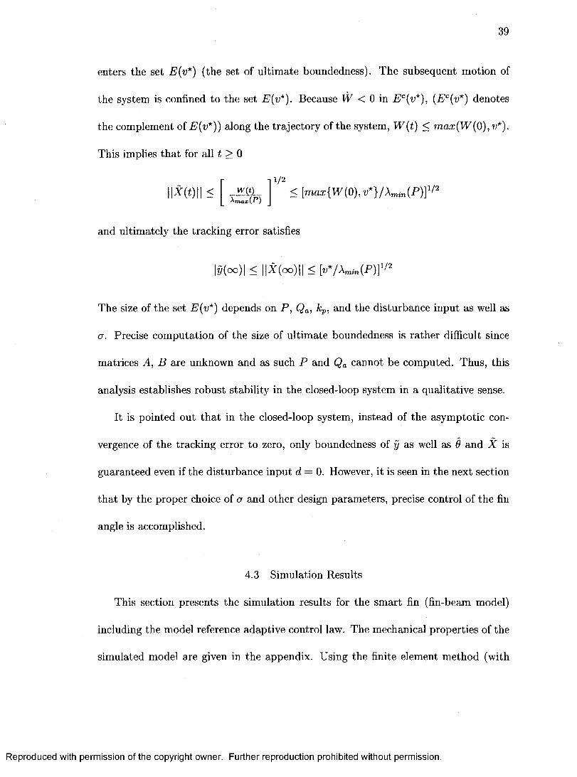
39
enters the set E{v*) (the set of ultimate boundedness). The subsequent motion of
the system is confined to the set E{v*). Because hF < 0 in E^{v*), (E‘ {v*) denotes
the complement of E{v*)) along the trajectory of the system, W(t) < max{W (0), w*).
This implies that for all t > 0
1 /2
< {max{W{0),v*}/Xmin{P)Y^‘Tna.x{P)
and ultimately the tracking error satisfies
|y(oo)| < ||X(00)|| < [ v * / X m i n { P ) ? ^ ^
The size of the set E{v*) depends on P , Qa, kp, and the disturbance input as well as
cr. Precise computation of the size of ultimate boundedness is rather difficult since
matrices A, B are unknown and as such P and Qa cannot be computed. Thus, this
analysis establishes robust stability in the closed-loop system in a qualitative sense.
It is pointed out that in the closed-loop system, instead of the asymptotic con
vergence of the tracking error to zero, only boundedness of ÿ as well as 6 and X is
guaranteed even if the disturbance input d = 0. However, it is seen in the next section
that by the proper choice of a and other design parameters, precise control of the fin
angle is accomplished.
4.3 Simulation Results
This section presents the simulation results for the smart fin (fin-beam model)
including the model reference adaptive control law. The mechanical properties of the
simulated model are given in the appendix. Using the finite element method (with
Reproduced with permission of the copyright owner. Further reproduction prohibited without permission.

40
n= 5 elements), a state-variable representation of the fin-beam model of dimension
of 20 is obtained for simulation. Of course the designed adaptive control system is
independent of the order of the fin-beam model. The reference command trajectory
is obtained using a first order command generator, with values Am = —6 , Bm = 6 ,
Cm = 1- The values T = 5 0 0 0 0 0 0 2»), Fp = 0 and a = 2 x 10~ are used for
simulation. The damping coefficient is taken as C = 0.005. Simulation results are
shown for different fin angle commands. Based on the lowest frequency of the flexible
modes (Qj = 53.343rad/sec), the value of y = 0.5 is selected which is less than
26iDi = 0.53. The initial estimate of ù{0) are taken as [—10,0,0]^.
4.3.1 Adaptive Control: 6 = 3°, a = —5“ and -t-5°
Simulation results for a fin angle command of 5“ for angles of attack a: = — 5® and
a = +5° are shown in Figure 4.1 and 4.2, respectively. It is observed that the fin angle
asymptotically converges to the desired value in about 5 seconds. In the steady state,
the control input u — u* {u* denotes the value in the equilibrium condition) needed
to deflect the fin to an angle of 5° for a = —5® is 1000 volts and a = +5° is 1060 volts.
The deflections at other points on the beam remain bounded during the maneuver
and converge to constant values, in both the cases. Note that Wi+i{t) > Wi{t) in the
figure. In spite of the cr-modification, in the adaptation law, the tracking error is
almost zero in about 10 seconds. We note that there is no overshoot in the fin angle
trajectory and the control input never exceeds u*, the voltage required to maintain
0 = 5“ in the equilibrium condition. The estimated parameters remain bounded and
converge to certain constant values.
Reproduced with permission of the copyright owner. Further reproduction prohibited without permission.

41
4.3.2 Adaptive Control: 9 = —10°, a = —10° and +10°
Figure 4.3 and Figure 4.4 show the simulation results for fin angle command of
—10°, for the angles of attack —10° and +10°, respectively. These results show that
the fin angle control is achieved in about 5 seconds. We observe that for larger fin
angle command the control magnitude required is larger as expected. The control
magnitude required for the deflection of —10° is almost twice the voltage needed for
5°. It is also interesting to see that there is no overshoot for the flexible modes and
they reach their equilibrium values, in both the cases. All the estimated parameters
converge to constant values.
4.4 Conclusion
In this chapter, the control of rotation angle of a smart projectile fin. The model of
the fin-beam system includes the aerodynamic moment which is a function of angle of
attack of the projectile. A model reference adaptive controller, based on the command
generator tracker concept was designed. Only the fin angle and its derivative were
required for feedback. Interestingly, the structure of the adaptive controller is simple
and does not depend on the dimension of the fin-beam model. Simulation results
show that the designed adaptive control system accomplishes precise fin angle control
in spite of uncertainties in the fin-beam parameters and the aerodynamic moment
coefficients.
Reproduced with permission of the copyright owner. Further reproduction prohibited without permission.

42
E>>
wcgÜ<DQ
X 1 0 -
Time (sec)
Time (sec)10
Time (sec)0
____ O - 0 . 0 0 2
■a
/ « 4
--0.004 /p /t -0.006 LUCO-0.008
//
"q —0 . 0 1
« ± - 0 . 0 1 21 /
10Time (sec)
1500 8000
6000O 1000
4000
2000
-500 -200010
Time (sec)Time (sec)
Figure 4.1: Adaptive Control: 6 = a -5°
Reproduced with permission of the copyright owner. Further reproduction prohibited without permission.
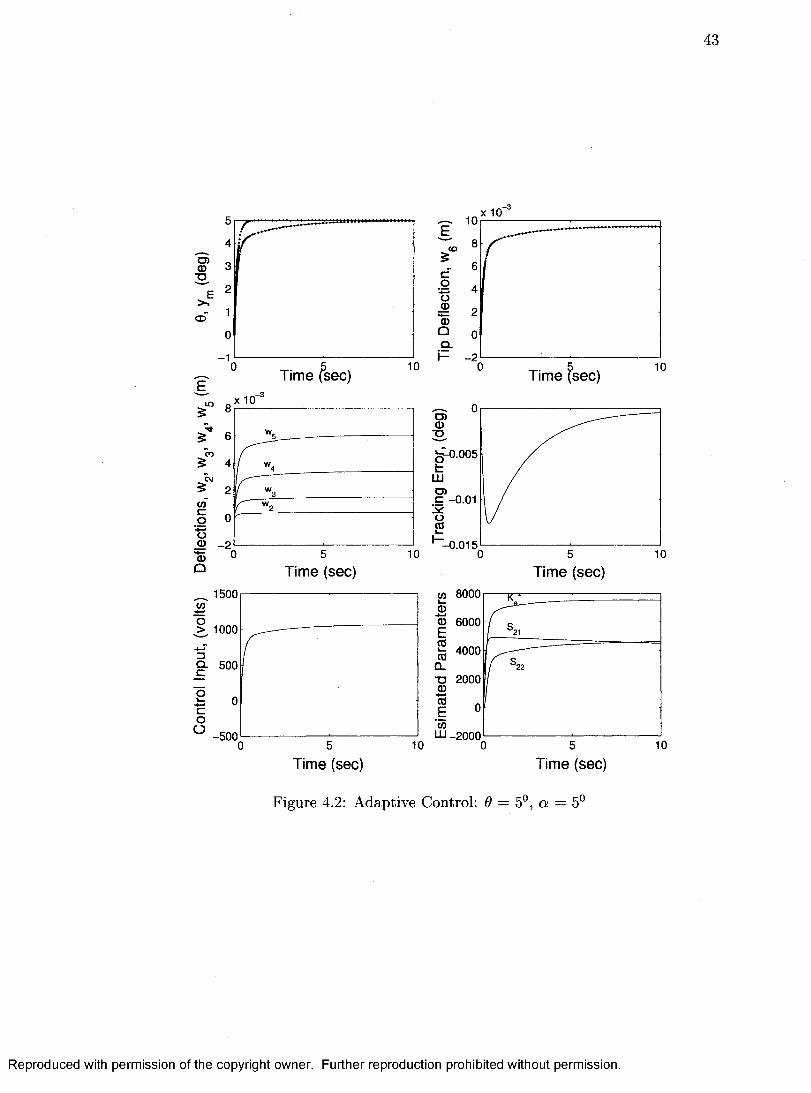
43
Time fsec),x 10
6
5 ” 4
sT 2<0
O 0
•s © -2 © ' Q Time (sec)
10-0.015
1500
> 1000
O- 500
-500
Time (sec)
Time fsec)
0.005
c -0.01
Time (sec)
Figure 4.2; Adaptive Control: 6
tn 8000
© 6000
T J 2 0 0 0
HI -2000
Time (sec)
Reproduced with permission of the copyright owner. Further reproduction prohibited without permission.

44
,-3X 10
- 4® -10
® -6O -15g-•“ -20
-8
-1 010 Time fsec)Time (sec)
.-3 -3X 10 X 10in 8
T J 6CO
4CD
C -1 0 2
® -15 0Time (Sec) 0 10Time (sec)
500
CL-1000
7 : -1500
C -2000
■2500
Time fsec)
v> 10000
B 8000 oE2CO
6000
4000
"S 2000
I “UJ -2000
Time sec)
Figure 4.3: Adaptive Control: 9 = —10°, a = —10°
10
Reproduced with permission of the copyright owner. Further reproduction prohibited without permission.

45
xIO
c -5
-1 0-6
Q -15 Q.i- -20
-8
-1010Time (lec) Time (sec)
,-3 ,-3X 10 X 1 0in O)
co-5 LU
D>CM
-15Time fsec)Time (sec)
1000 8000
500 6000
4000
73 2000-1000
5 -1500
-2000 LU-2000Time (sec)Time (sec)
Figure 4.4: Adaptive Control: 9 = —10”, a — 10”
Reproduced with permission of the copyright owner. Further reproduction prohibited without permission.

CHAPTER 5
ADAPTIVE SERVOREGULATOR
In chapter 4, an adaptive controller based on the command generator tracker concept
was designed. The synthesis of this controller required tuning of three parameters of
the adaptive loop. This required sigma or dead-zone modification of the adaptation
rule in order to avoid parameter divergence. The modification of the adaptation rule
may sometimes give terminal tracking error. This chapter deals with an adaptive
servoregulator designed for the control of the fin angle and the rejection of the dis
turbance input (aerodynamic moment). It is assumed that the system parameters
are completely unknown and that only the fin angle and its derivative are measured
for synthesis. A linear combination of the fin angle and fin’s angular rate is chosen
as the controlled output variable. Here the controller requires tuning of a single gain
and unlike in chapter 4, the controller is capable of rejecting the aerodynamic distur
bance torque without any adaptive law modification. In the closed-loop system, the
fin angle asymptotically converges to the target fin angle generated by a command
generator.
46
Reproduced with permission of the copyright owner. Further reproduction prohibited without permission.

47
5.1 Adaptive Servocontrol Law
In this section, an adaptive servoregulating controller will be designed. Defining
the state vector x = {rj , a state variable representation takes the form
X02n x2n I 2 n x 2 n
-D2 -2D9.X +
02nxlu +
02nxl
A Ax + Bu + Fv
We select the controlled output variable as
y = ( 0 + \ 6 )
= Cm + ACoi) = Cx
(5.1)
(5.2)
where A > 0 is a design parameter. From Eq. (5.2), one obtains
ÿ(g) = C(gL - A)-^BÙ(g) + C(gL - A)-^FÛ(3)
A np{s)u{s) + nf{s)v{s) dp{s)
(5.30
(5.40
where s is the Laplace variable and u and v denote Laplace transforms of u and v
respectively, and
It is easily seen that
np{s) = Cadj{sl — A)B
rif{s) = Cadj{sl — A)F
dp{s) = det{sl — A)
2ndp{s) = + 2 ÇfliS +
2— 1
(5.5)
Reproduced with permission of the copyright owner. Further reproduction prohibited without permission.

48
is a Hurwitz polynomial. Furthermore, computing the polynomial np{s) for this
model, one finds that it is a Hurwitz polynomial. Therefore, the transfer function
{rip{s)/ dp{s)) is minimum phase.
The tracking error ei — y — ym is
- Vmis) (5.6)dp\S) dp( sj
where y^ is the constant reference trajectory is constant. For a given angle of attack,
the aerodynamic moment v — mao{o:) acts as a constant disturbance input and it
must be rejected by the controller. In order to eliminate this unknown disturbance
term v, let us filter each side of Eq. (5.6) with ( j |^ ) , where yu > 0. For constant
signals v and one has su = 0 and = 0. Therefore, the filtered equation Eq.
(5.6) yields
We note that we have ignored the exponentially decaying signals in Eq. (5.7).
Defining the filtered input signal as
Uf{s) = (5.8)
Eq. (5.7) can be expressed as
" - <•■•>
= H(s)ü,(s)
In view of Eq. (5.9), it is sufficient to derive a control law Uf{t) such that the tracking
error ei{t) is regulated asymptotically to zero.
Reproduced with permission of the copyright owner. Further reproduction prohibited without permission.

49
For the fin-beam model, H{s) is minimum phase because np{s) is Hurwitz and
fx > 0. Moreover, by the choice of the output y, the transfer function has relative
degree one. As such using a simple argument from the root-locus technique, it is
easily seen that a negative feedback law of the form
Uf{t) — —KgCi (5.10)
can stabilize the system Eq. (5.9), where Kg > 0 . Indeed, as Kg tends to oo, the
root loci of the closed-loop poles converge to finite stable zeros of H{s) and one of
the pole tends to —oo along the asymptote with angle tt. This is interesting, because
it is an extremely simple control law and yet it accomplishes error regulation and
disturbance (n) rejection.
Consider a minimal realization of H{s) given by
Xa — A(iX(i Bg Uj (5.11)
— CgXg
where A„, Bg and Cg are appropriate matrices. Of course, these matrices are not
required for synthesis. Since H{s) is minimum phase with relative degree one, it
follows that there exists a gain K* > 0 such that [27]
f (A - -F (A - = -Q < 0
_Pga = C^ (5A2)
where P and Q are positive definite symmetric matrices. However, K* is not known.
Let K be an estimate of K* and consider an output feedback law
Uf = —Kci (5.13)
Reproduced with permission of the copyright owner. Further reproduction prohibited without permission.

50
The goal is now to adaptively tune K to accomplish error regulation. Using Eq.
(5.13) in Eq. (5.11) gives
= (A. - + (jC B .C .z. - R-g.ei) (5.14)
Defining the parameter error K — K* — K, Eq. (5.14) gives
Xa = A x a + KBgCi (5.15)
where À = (A„ — K^BgCa) is a Hurwitz matrix since Eq. (5.12) holds.
For the derivation of the adaptation law, consider a quadratic Lyapunov function
W ^ x l P x a P u k ^ (5.16)
where > 0. The derivative of W along the solution of Eq. (5.15) is given by
W = (PA. + A lP )z . + 2 z lP K g .e i + 2-yKÆ (5.17)
Using Eq. (5.12) in Eq. (5.17) and noting that XgPBg = XgCj = ei gives
W = + 2Æ('yÆ + e ) (5.18)
In order to eliminate K form, the adaptation law is chosen as
k = - K = - T ^ e \ (5.19)
Substituting Eq. (5.19) in Eq. (5.18) gives
W ^ -x lQ x a < 0 (5.20)
Since W{xa,K) is positive definite and W < 0 , X g and K are bounded. Further
more, invoking Barbalat’s Lemma[23, 26], one can establish that Xg tends to zero
which in turn implies that ei = CgXg converges to zero.
Reproduced with permission of the copyright owner. Further reproduction prohibited without permission.

51
The control input u{t) now can be obtained using Eq. (5.8). In view of (5.8), one
has
Û = ( ^ (5.21)
which yields
u{t) = Uf{t) + IJ, [ Uf{t)dT (5.22)J o
Using Uf{t) = —K{t)ei{t) in Eq. (5.22) gives
u{t) = -K{t)ei{t) - yu / K{r)ei{T)dT (5.23)J o
For a constant K, the control input simply uses proportional and integral feedback
of the tracking error.
5.2 Simulation Results
This section presents the simulation results for the smart fin (fin-beam model)
including the model reference adaptive control law. The mechanical properties of
the simulated model are given in the appendix. Using finite element method (with
n=5 elements), a state-variable representation of the fin-beam model of dimension
20 is obtained for simulation. The aerodynamic moment Eq. (2.13) is chosen for
different angles of attack of the projectile based on the CED analysis. By a linear
approximation of the data obtained by the CFD analysis, the parameters of the
aerodynamic moment are found to be niao = —0.0022, = -f0.0005 for a — —5® and
TUoo = —0.0028, Pa = 0.01 for a = +5°. The value of 7 and p is chosen to be 0.00001
and 100 respectively. The initial value of K is taken as 500. The damping coefficient
is taken as ( = 0.005. Simulation results are shown for different fin angle commands.
Reproduced with permission of the copyright owner. Further reproduction prohibited without permission.

52
5.2.1 Adaptive Servo Control; 9 = b°, a = —5° and a = 5°
Figure 6.1 and Figure 6.2 show the simulation results for fin angle of 5", with angles
of attack —5° and +5°. It is observed that the fin angle asymptotically converges to
the desired value in 1 second. The control input needed for the fin to deflect to an
angle, 9 = 5° with angle of attack, a = —5° is about 1100 volts, while that with
o; = 5“ is more than 1200 volts. We observe that for larger fin angle command the
control input needed is much larger. We also observe that there is no overshoot for
the flexible modes and they reach their equilibrium values at the steady state, in both
the cases.
5.3 Conclusion
An adaptive servoregulator was designed for the control of fin angle. Simulation
results show that the designed adaptive control system accomplishes precise fin angle
control in spite of uncertainties in the fin-beam parameters and the aerodynamic
moment coefficients.
Reproduced with permission of the copyright owner. Further reproduction prohibited without permission.

53
0.008
0.006g§ 0.004
0.002
X 10
2 4Time (sec)
2 4Time (sec)
-2
Time (sec)
1200
ôiooo
^ 800
È 600
400
O 200
Time (sec)
800
©750
700
©550
500
xlOE
CM$CO
oü©©Q -5
Time (sec)
Time (sec)
Figure 5.1: Adaptive Servo Control: 6
2 4Time (sec)
a
Reproduced with permission of the copyright owner. Further reproduction prohibited without permission.

54
CD
U_
Time (sec)X 10
to
-2
Time (sec)
1200
^1000
5 800Q.— 600
400
200
Time (sec)
S 750
« 600
% 550
0.01
=tp008
c 0.006 o© 0.004 ©
0.002
2 4Time (sec)
X 10E
CO
COco©©o
-5
Time (sec)
2 - 0 .5
2 4Time (sec)
2 4Time (sec)
Figure 5.2: Adaptive Servo Control: 6 = 5 , a = 5°
Reproduced with permission of the copyright owner. Further reproduction prohibited without permission.

CHAPTER 6
VARIABLE STRUCTURE ADAPTIVE CONTROL
The adaptive control systems designed in the previous chapters require integral type
adaptation schemes. These adaptation schemes are not robust unless some modifi
cations in the update laws are done. Certainly it is useful to explore other adaptive
designs in which dynamic adaptation of parameters is avoided.
In this chapter, based on the variable structure model reference adaptive control
(VS-MRAC) theory, a new control system for the control of a projectile fin is designed
in this chapter. For the derivation of the control law, it is assumed that the parameters
in the model are unknown, and only the fin angle is measured for feedback. Control
using only the fin angle measurement is very practical since measurement of flexible
modes is not easy. However, it is assumed that an upper bound on the uncertain
functions is given. Significant advantages of VS-MRAC designs are: nice transient
behavior, disturbance rejection capability, and insensitivity to plant nonlinearities or
parameter variations.
55
Reproduced with permission of the copyright owner. Further reproduction prohibited without permission.

56
6.1 Fin Model and Control Problem
Defining the state vector Xf = E a state variable representation
takes the form
0 2 n x 2 n ^ 2 n x 2 n 0 2 n x l 0 2 n x lX f =
- Q 2 - 2 D Ç I
X -F
B x
u -F
F x
= AfXf + bfU + Fv
We select the controlled output variable as
y = 6 = hfXf
(6 .1)
(6 .2)
Let ym be a smooth reference trajectory generated by a reference model. We are
interested in deriving a VS-MRAC control law u{t) such that the fin angle tracking
error
( 0 — y ~ Vm
asymptotically tends to zero and the elastic modes remain bounded during maneuver.
Furthermore, for a constant set point control of fin angle, it is desired that the fiex-
ible modes converge to their equilibrium values. By suitable choice of the reference
trajectory ym, desirable fin angle control is accomplished.
Consider the input-output representation of the system Eq. (6.1) given by
y{s) = h f{sl - Af) ^bfu(s) + h f{sl - A f) ^Fv{s)
A kj,np{s)u{s) + nf{s)v{s) dp{s)
where s denotes the differential operator or the Laplace variable.
(6.3)
(6.4)
Reproduced with permission of the copyright owner. Further reproduction prohibited without permission.
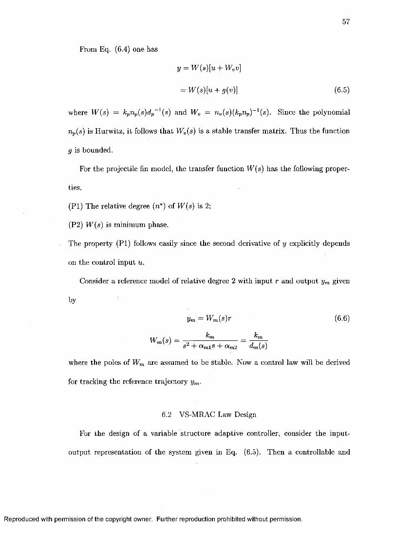
57
From Eq. (6.4) one has
y = W{s)[u + WyV]
= IF(s)[tt + 5'(n)] (6.5)
where hF(s) = kpnp{s)dp~^(s) and = riv{s){kpnp)~^{s). Since the polynomial
rip(s) is Hurwitz, it follows that W„(s) is a stable transfer matrix. Thus the function
g is bounded.
For the projectile fin model, the transfer function W (s) has the following proper
ties.
(PI) The relative degree (n*) of VF(s) is 2;
(P2) W(s) is minimum phase.
The property (PI) follows easily since the second derivative of y explicitly depends
on the control input u.
Consider a reference model of relative degree 2 with input r and output ym given
by
Vm = W m { s ) r (6.6)
H“ Olml^ "F Olm2 ( m( )
where the poles of Wm are assumed to be stable. Now a control law will be derived
for tracking the reference trajectory ym-
6.2 VS-MRAC Law Design
For the design of a variable structure adaptive controller, consider the input-
output representation of the system given in Eq. (6.5). Then a controllable and
Reproduced with permission of the copyright owner. Further reproduction prohibited without permission.

58
observable representation of Eq. (6.5) is given by
X = A x F b{u + g{v)) (6 .7)
y = h^x
It is pointed out that the knowledge of matrices A, b, h and g are not required for
the design of the control system.
For the synthesis of the controller, now the following filters are introduced.
Cj\ — FuJi + uu
(1)2 — F u)2 + Dy (6 .8)
where Wi, W2 E ,
~^n-2 — •••• — Ao
....0
where I and 0 denote identity and null matrices of appropriate dimensions and A, are
coefficients of the polynomial
A(s) — s” F A^_2s” F ... F AiS F Aq — det(s/ — E)r,n-~2 (6.9)
Define w = [o;f, y,(vj, r]^ € The control law is to be synthesized using only the
regressor vector w.
Since kF(s) and Wm{s) have same relative degree 2, for g{v) = 0, there exists a
unique constant vector 9* = [9^ , 9y , 6^^, 9*] € such that the transfer function
Reproduced with permission of the copyright owner. Further reproduction prohibited without permission.

59
of the closed-loop system with the control input
+ ^ !/ +
matches the transfer function Wm(s) exactly, i.e.,
y = hF(s)u = W{s)0*^uj = Wm{s)r
For model matching, the parameter vector 6* must satisfy [25,26]
— k m / k p
(6 .10)
(6 .11)
(6.12)
6/*^a(s)dp(s) + kp{el^a{s) + 0*A(s))np(s) = A(s)dp(s) - np(s)A(s)dm(s) (6.13)
where a(g) = ...s, 1] and 9 denotes the k^ element of 9*.
Solving Eq. (6.13) gives the parameter vector 9*.
Define k* = {9*)~ = kp/km, and û = u — u*. For the fin-beam model, kp > 0 and
the chosen parameter km is positive, and therefore both k* and 0* are positive.
Defining the vector = (x'^, u J , G the composite system Eqs. (6.7)
and (6 .8) can be written as
X — AaX + baU + bgg (6.14)
where
Aa =
A 0 0 b b
0 F 0 , K — V , bg = 0
0 F 0 0
0
Reproduced with permission of the copyright owner. Further reproduction prohibited without permission.
60
Define
0 I 0
y hF 0 0
CÜ2 0 0 I
P X (6.15)
Now adding and subtracting baU* in Eq. (6.14) and using Eqs. (6.10) and (6.15),
gives
X = AcX + bcK*ü + bcT + bog (6.16)
where Ac = + ba[0^ , 9*, 9*^]P and be — 9*ba- For u — u* (i.e. ü = 0) and 5 = 0,
one has Wm — — Ac)” 5c- Therefore, the output of Eq. (6.16), ignoring the
exponentially decaying signals due to initial conditions, which is not essential for
derivation, can be written as
y = Wm{s)r + K*Wm{s)u + gc{v) (6.17)
where gc = Wm{s)g, Wm{s) = h^{sl — Ac)~^bg. Here Wm(s) is a stable transfer
function, and therefore, gc is bounded for any bounded function g.
Since Wm — h^{sl — A)^^bc, a non-minimal realization of the reference model
(Eq. (6 .6)) is
where Xm. E
Xm — AeXm F bcT
Vm — X m
(6.18)
Reproduced with permission of the copyright owner. Further reproduction prohibited without permission.
61
Let the state vector error be e = X — Xm- Subtracting Eq. (6.18) from Eq. (6.16)
gives the error equation and the tracking error {y — ym) given by
é = AcS + bciFü + bgQ (6.19)
Cq = h^e
Using Eq. (6.19), the output tracking error can be written as cq = K,*Wm{s)ü + g^v ) .
For the synthesis of the controller, its is essential to introduce a chain of auxiliary
errors (e^). Since the relative degree n* of the reference model is two, IFm(a) is not
SPR (strictly positive real). To circumvent this difficulty, a polynomial L{s) given by
L{s) = ^-^ ,< 5 > 0
is chosen so that the tarnsfer function Wm{s)L{s) is SPR. Now, we introduce the
following set of filtered signals;
Xo = L ~ ^X i
where %i = «, & = w and ...,^2n))^ E {i = 0,1). These signals are used
to generate a chain of auxiliary error signals e'^i = 0,1). Based on the results of Refs.
[30,32], the complete algorithm for the fin angle control is summarized in Table 1.
Reproduced with permission of the copyright owner. Further reproduction prohibited without permission.

62
Table 1; VS-M RAC Algorithm
Auxiliary Errors
Va — Wm L [%() L
^0 — y ym, ^0 ~ ya
Cl = (1*0 ) 6 9 L ('^l)
Modulation Functions fo > R \ Xo — 1 + Zly=i doj 1 1 +5o + Co
/ i > 1 1 +9i + Cl
Control Laws
Ui = f iSgn{e'i),i:= 0,1
Vj — U\ “f" '^nom
'( nom — ^nom^
In the above table, 6nom and Knom F 0 are chosen nominal values of the parameters
Q* and K*, respectively, cq > 0 ,ei > 0 , and the upper bounds 6ij (i = 0 , 1 and
j = 1,..., 2n), R, and g, {i = 0 , 1) are defined as
9oj ^ P \ dj 9j,nom I) 9 i j >1 6 j 9j,nom |; ^ ^ | 5 1 |
t>o t>o
5i > sup6>;Wm'^gc = sup6>;Wm“ W „ g t> 0 o o
(6 .20)
Reproduced with permission of the copyright owner. Further reproduction prohibited without permission.

63
nom
nom
FilterFilter
ProjectileFin
ReferenceModel
Figure 6 .1: VSMRAC Model
where p = K*/Knom- Note that {knomWmL)^^Wm is a strictly proper stable transfer
function, 6*W~^Wm is a proper stable transfer function, and g is a bounded signal.
Note that pa can be interpreted as a predicted output error and hence is a prediction
error [30]. The complete closed-loop system is shown in Fig. 6.1.
The equivalent control {uo)eg can be obtained by setting = 0 in the dynamical
system governing the error e], and can be approximately obtained from uq by means
of a low-pass filter (averaging filter) with high enough cut-off frequency denominated
averaging filter [31]. The inclusion of such averaging filters in the stability analysis
has been considered in Ref. [30].
Reproduced with permission of the copyright owner. Further reproduction prohibited without permission.

64
Now consider the VS-M RAC law of Table 1. Then for any trajectory the closed-
loop system has the following properties :
a) The errors e- {i = 0,1) all converge to zero in finite time;
b) The fin angle tracking error Cq converges exponentially to zero.
From Table 1, we find that the control law is a discontinuous function of e\. It is
well known that this discontinuity in the control law causes undesirable control chat
tering. For avoiding control chattering, one uses a smooth continuous approximation
of the switching functions. For this, one replaces u = sgn{el) hy u — sat{e'j), where
sat{rj) is defined as sat{rj) = sign{r]) if | (77) |> A, and sat(r]) = (g/S) if | (77) |< A.
Here A is the bounded layer thickness.
From Table 1, we observe that for the synthesis of the control law, it is essential to
compute the modulation functions f{. Of course, these functions fi can be computed
on-line using signals and %o, and the bounds gi on uncertain functions. However,
implementation of this control law using on-line computation of the bounds fi is
extremely complicated. A simple control law can be synthesized by using constant
overestimated values of the modulation functions. The simplified control system has
been termed as the Relay VS-M RAC [30].
6.3 Simulation Results
In this section, simulation results for the closed-loop system with the control law
derived in Table 1 are presented. The closed-loop system is shown in Figure 6.1.
The mechanical properties of the simulated model are given in the appendix. Using
Reproduced with permission of the copyright owner. Further reproduction prohibited without permission.

65
the finite element method (with n=5 elements), a state-variable representation of the
fin-beam model of dimension of 20 is obtained for simulation.
The reference model is chosen as
where is 0.1. We choose L = {s + Xm)/^m so that Wm.L is SPR. For the
computation of n„om = the nominal value of 9 was arbitrarily chosen as
9nom = (0,..., 0,1)^ G giving Unom ~ 1'■ TMs is rather an unfavorable choice
of estimate of 9*. In the saturation function, the boundary layer thickness set to
A = 0.5. A simplified relay type controller was synthesized by using constant modu
lation functions as /o = 1000000 and fx — 1000000.
6.3.1 Adaptive Control: 0 = 5°, a = —5°, 5°
Simulation results for a fin angle command of 5“ for angle of attack a = — b*’ are
shown in Figure 6.2. Figure 6.3 shows the simulation results for fin angle command
of 5° with angle of attack, a = 5°. It is observed that the fin angle asymptotically
converges to the desired value in less than 1 second in both the cases. In the steady
state, the control input needed to deflect the fin to an angle of 5° for a — —5° is
around 1000 volts. The deflections at other points on the beam remain bounded
during the maneuver and converge to constant values. The tracking error is of the
order of 10“ . We note that there is no overshoot in the fin angle trajectory and
the control input never exceeds u*, the voltage required to maintain 0 = 5° in the
equilibrium condition.
Reproduced with permission of the copyright owner. Further reproduction prohibited without permission.
66
6.4 Conclusions
Based on the variable structure model reference adaptive control theory, a new
control law for the control of fin angle of a projectile fin was presented. In the fin-beam
model, disturbance input was assumed to be present. A variable structure model ref
erence adaptive control system was synthesized using only measurement on the fin
angle and measurement of other flexible modes was not needed for control. Inter
esting, unlike usual adaptive controller, the derived VS-MRAC system does not have
integral type adaptation law for updating the parameters of controller. This structure
of adaptive controller has significant advantage over other adaptive schemes, since in
this case controller parameter divergence cannot occur. In the closed-loop system, fin
angle tracked the reference trajectory, and stabilization of flexible modes was accom
plished. Extensive simulation results were presented which showed good transient
characteristics of the designed controller in spite of the presence of uncertainties in
the system parameters and aerodynamic disturbance input.
Reproduced with permission of the copyright owner. Further reproduction prohibited without permission.

67
0.016
0.008COT3 4f 0.006
3O) m 0.0042
0.0021 Q .
00 2 4
Time (sec)6
Time (sec),-3X 10 X 10
20
in n
- 2 -56
Time (sec)Time (sec)
1200
o 1000
800Q.
600
400
200
Time (sec)
X 10
Time (sec)
Figure 6.2: Variable Structure Control: ^ — 5°, a = —5°
Reproduced with permission of the copyright owner. Further reproduction prohibited without permission.

68
O)
u_
Time (sec)X 10
m
-2
Time (sec)
1200
o 1000
800
600
400
200
Time (sec)
.-3X 10
CO
Q.- 2
Time (sec)X 10
2 4Time (sec)
1-3X 10
3 -0 .2-§" -0.4
- 0.6
- 1.2
Time (sec)
Figure 6.3: Variable Structure Control: 0 = 5®, o; = 5®
Reproduced with permission of the copyright owner. Further reproduction prohibited without permission.

CHAPTER 7
CONCLUSION
This thesis considered the control of rotation angle of a smart projectile fin. The
flexible beam with a piezoelectric active layer was used for rotating the fin. In the
second chapter, the mathematical model of the fin-beam system was described and a
state-variable model was obtained using the finite element method.
In the third chapter, a state feedback adaptive control law was designed for the
trajectory control of the fin angle. This was followed by the design of an adaptive
control system using only output feedback. The effect of aerodynamic moment was
not considered here. In the closed-loop system, asymptotic trajectory tracking of the
fin angle was accomplished. Simulation results showed that trajectory control of the
fin angle was accomplished in spite of large uncertainties using the state as well as
output feedback and the flexible modes remain bounded during maneuvers.
The fourth chapter considered a model reference adaptive control for the projectile
fin. This model included the aerodynamic moment which is a function of angle of
attack of the projectile. Based on the command generator tracker concept, a model
reference adaptive fin angle controller was designed. The structure of the control
system designed was independent of the dimension of the flexible fin-beam model. In
69
Reproduced with permission of the copyright owner. Further reproduction prohibited without permission.

70
the clsed-loop system, the controlled output variable tracked the reference trajectory
and the fin angle asymptotically converged to the desired value. The elastic modes
converged to their equilibrium values. Simulation results presented showed that, the
fin angle was precisely controlled in spite of uncertainties in the fin-beam parameters
and the aerodynamic moment coefficients.
In the fifth chapter, an adaptive servoregulator was designed for the control of the
fin angle and the rejection of the disturbance input (aerodynamic moment). It was
assumed that the system parameters are completely unknown and that only fin angle
and its derivative are measured for synthesis of the control law. A linear combination
of the fin angle and the fin’s angular rate was chosen as the controlled output variable.
Computer simulations performed showed that in the closed-loop system, the fin angle
was precisely controlled in spite of uncertainties in the fin-beam parameters and the
aerodynamic moment coefficients.
Finally in chapter 6 , a control system was designed for the control of the flexible
beam based on the theory of variable structure model reference adaptive control (VS-
MRAC) using only input and output signals. It was assumed that an upper bound on
the uncertain functions is given. This adaptive controller has significant advantage
over other adaptive schemes, since in this case controller parameter divergence cannot
occur. Extensive simulation results presented showed good transient characteristics
of the designed controller in spite of the presence of unmodeled dynamics, uncertainty
in system parameters, and disturbance input.
The real time control of the fin using adaptive servoregulator (described in chapter
Reproduced with permission of the copyright owner. Further reproduction prohibited without permission.

71
5) has been done in the laboratory. The reference fin angle was set to 3° during this
real time simulation, as voltage was constrained to a maximum value of +1500 volts
giving maximum angle of 4.5*’. The basic filter of the form was used to reduce
the noise of the signal coming from the encoder. Test results showed that fin angle
was controlled very close to the target fin angle of 3®. It is seen that the control of fin
using adaptive servoregulation is very practical than any other methods developed in
this thesis. Higher fin angles can be achieved by choosing different configurations of
the actuator (like biomorph configuration). The effect of aerodynamic moment is not
yet included into real time simulation, but wind tunnel test is of interest in future.
Reproduced with permission of the copyright owner. Further reproduction prohibited without permission.

72
APPENDIX
SYSTEM PARAMETERS
The mechanical parameters for simulation in chapter 3 are taken as
pb — 2 ,700{kg/m^) pp = 7, bOO{kg/m^)
El, = 970GPa Ep = 63GPa
L = 140mm b = 25mm
hb = 0.5mm hp = 0.127mm
^31 = 1.8E' — I0{m/volt)
By a linear approximation of the data obtained by the CED analysis, the param
eters of the aerodynamic moment are found to be
m^o = —0.0022, Pa = +0.0005 for a = —5°
ntiao — —0.0028, Pa — + 0.01 for oc H— 5°
The controller parameters in chapter 3 are chosen as
c = 0.707 U n = 50
^ = 5 Cg = 20
P = hox2o p(0) = 0.309
Oq — Ogoxl — 2
yr(0) = 0 A = 4.
Reproduced with permission of the copyright owner. Further reproduction prohibited without permission.

73
The mechanical parameters for simulation in chapters 4, 5 and 6 are taken as
Pb = 8 ,300{Kgfrrî^) Pp = 7 ,500(%g/m^)
Eb = 95GPa Ep = 15.89GPa
L — 109.4mm b = 25mm
hb = 0.4mm hp = 0.3mm
ds3 = 170P — 12{m/volt)
The controller parameters used for simualation in chapter 4 are
= - 6 Pm = 6 Cm = 1
r = 5 0 0 0 0 0 0 ( 7 2 » x 2 n )
Fp = 0 (7 = 2 X 10~®
Ci = 0.005 p — 0.5
z>(0) = [10 ,0 ,0 f
The controller parameters chosen for simulation in chapter 5 are
7 = 0.00001 p = 100
 = 500 a = 0.005
Reproduced with permission of the copyright owner. Further reproduction prohibited without permission.

REFERENCES
1. Batra, R. G., Ghosh, K., “Deflection Control During Dynamic Deformations
of a Rectangular Plate Using Piezoceramic Elements”, AIAA Journal., Vol.33,
No.8 , 1995, pp 1547-1548.
2. Lin, C. C., Hsu, C. Y., Huang, H. N., “Finite element analysis on deflection
control of plates with piezoelectric actuator”. Composite Structure., Vol.35,
1997, pp 423-433.
3. Barrett, R., “Active plate and missile wing development using directionally
attached piezoelectric elements”, AIAA Journal., Vol.32, No.3, 1994, pp 601-
609.
4. Bent, A. A., Hagood, N.W., J.P. Rodgers., “Anisotropic actuation with piezo
electric fiber composites”, Journal of Intelligent Materials Systems and Struc
tures., Vol.6 , No.3, 1995, pp 338-349.
5. Rabinovitch. O., Vinson, J., “On the design of piezoelectric smart fins for flight
vehicles”. Smart Materials and Structures., Vol.12, 2003, pp 686-695.
6 . Rabinovitch, O., Vinson, J., “Smart fins; Analytical modeling and basic design
concepts”, Mech. Adv. Mater. Struct., Vol.10, 2003, pp 249-269.
74
Reproduced with permission of the copyright owner. Further reproduction prohibited without permission.

75
7. Yim, W., Singh, S. N., “Variable structure adaptive control of a cantilever beam
using piezoelectric actuator”, Journal of Vibration and Control., Vol.6 , 2000,
pp 1029-1043.
8 . Yim, W., Singh, S. N., M. Trabia., “Adaptive Control of Projectile Fin Angle
Using Piezoelectric Beam Actuator”, Proceedings of SPIE Smart Structures
and Materials., 2004.
9. Bailey, T., Hubbard, J. E., “Distributed Piezoelectric-Polymer Active Vibration
Control of a Cantilever Beam”, Journal of Guidance, Control, and Dynamics.,
Vol. 8 , No.5, 1986, pp 605-611.
10. Baz. A., Poh, S., “Performance of an active control system with piezoelectric
actuator” . Journal of Sounds and Vibration., Vol.126, No.2, 1988, pp 327-343.
11. Tzou, H. S., “Distributed Modal Identification and Vibration Control of Con
tinual Theory and Applications”, ASME Journal of Dynamic Systems, Mea
surements, and Control., Vol.113, pp 494-499.
12. Choi, S. B., Lee, C. H., “Force Tracking Control of a Flexible Gripper Driven
by Piezoceramic Actuator” , ASME Journal of Dynamic Systems, Measurement,
and Control., Vol.119, pp 439-445.
13. Choi, S. B., Cheong, C. -C., Lee, C. H., “Position tracking control of a smart
flexible structure featuring a piezofilm actuator”. Journal of Guidance, Control
and Dynamics., Vol.19, No.6 , pp 1996.
Reproduced with permission of the copyright owner. Further reproduction prohibited without permission.

76
14. Shen, Y., Homaifar, A., “Vibration Control of Flexible Structures with PZT
Sensors and Actuators,” , Journal of Vibration and Control., Vol.7, 2001, pp
417-451,
15. Trabia, M., Yim, W., “Fuzzy Logic Control of Projectile Fin Angle Using Piezo
electric Actuator”, IMECE., 2004.
16. Hyland, D. C., Junkins, J. L., Longman, R. W., “Active Control Technology for
Space Structures”, Journal of guidance. Control and Dynamics., Vol.16, 1993,
pp 801-821.
17. Singh, S. N., “Robust Nonlinear Attitude Control of Flexible Spacecraft”, IEEE
Transactions on Aerospace and Electronic Systems., Vol.23, No.3, 1987, pp 380-
387.
18. Singh, S. N., Araujo, A. D., “Adaptive Control and Stabilization of Elastic
Spacecraft”, IEEE Transactions on Aerospace and Electronic Systems., Vol.35,
1999, pp 115-122.
19. Singh, S. N., Zhang, R., “Adaptive Output Feedback Control of Spacecraft with
Flexible Appendages by Modeling Error Compensation”, Acta Astronautica.,
Vol.54, 2004, pp 229-243.
20. Kelkar, A., Joshi, S., “Control of Nonlinear Multibody Flexible Space Struc
tures”, Springer, NewYork., 1996.
Reproduced with permission of the copyright owner. Further reproduction prohibited without permission.
77
21. Mufti, I.H., “Model Reference Adaptive Control for large structural systems”,
AIAA Journal of Guidance, Control and Dynamics, 1987, pp 507-509,
22. Spooner, J. T., Maggiore, M., Ordonnez, R., Passino, K. M., “Stable Adaptive
Control and Estimation for Nonlinear Systems” , John Wiley Sons., NY 2002.
23. Vidyasagar. M., “Nonlinear Systems Analysis”, SIAM Publications, NJ 2002.
24. Sastry, S., Bodson, M., “Adaptive Control”, Prentice Hall, NJ, 1989.
25. loannou, P. A., Sun, J., “Robust Adaptive Control” , PTR Prentice Hall, NJ,
1996.
26. Narendra, K. S., and Annaswamy, A. M., “Stable Adaptive Systems” , Prentice
Hall, NJ, 1989.
27. Kaufmann, H., Barkana, I., Sobel, K., “Direct Adaptive Control Algorithms”,
Springer-Verlag, New York., 1998.
28. Fradkov, A. L., Miroshnik, I. V., Nikiforov, V. O., “Nonlinear and Adaptive
Control of Complex Systems” , Kluwer Academic Publishers., 1999.
29. Annaswamy, A. M., Clancy, D. J., “Adaptive Control Strategies for Flexible
Space Structures”, IEEE Transactions on Aerospace and Electronic Systems.,
Vol.32, No.3, 1996.
30. Hsu, L., Araujo, A. D. and Lizzarralde, F., “New Results on Input/Output
Variable Structure Model Reference Adaptive Control: Design and Stability
Reproduced with permission of the copyright owner. Further reproduction prohibited without permission.

78
Analysis” , IEEE Transactions on Automatic Control, Vol.AC-42, No.3, 1997,
pp 386-393.
31. Utkin, V. I., “Sliding Modes and Their Applications in Variable Structure Sys
tems”, MIR, 1978.
32. Hsu, L., Araujo, A. D., and Costa,R. R., “Analysis and Design of I/O Based
Variable Structure Adaptive Control”, IEEE Transactions on Automatic Con
trol, Vol.AC-39, No.l, 1994, pp 4-21.
Reproduced with permission of the copyright owner. Further reproduction prohibited without permission.

VITA
Graduate College University of Nevada, Las Vegas
Smitha Mani
Local Address:1455 E Katie Ave, E15 Las Vegas, NV 89119
Home Address: Arunima Kottayam Kerala India 686019
Degrees:Bachelors of Technology, Applied Electronics and Instrumentation, 2001 College of Engineering, (Trivandrum)Kerala University, Kerala, India
Publications:Smitha Mani, et ah, “Adaptive Rotation of a Smart Projectile Fin using a Piezoelectric Flexible Beam Actuator”, Journal of Vibration and Control, Vol. 11,No. 8 , 2005 pp 1085-1102.
Smitha Mani, et ah. Adaptive Servo Regulation of a Projectile Fin Using Piezoelectric Actuator”, ASME International Mechanical Engineering Congress and Exposition, November 5-11, 2005, Orlando, FL.
Smitha Mani, et ah. Adaptive Control of a Projectile Fin Using Piezoelectric Elastic Beam”, Proc. of AIAA Guidance, Navigation and Control Conference
79
Reproduced with permission of the copyright owner. Further reproduction prohibited without permission.

80
and Exhibit, August 15-18, 2005, San Francisco, CA.
Smitha Mani, et ah. Direct Adaptive Control of a Smart Projectile Fin by Piezoelectric Flexible Beam Actuator”,Proc. of SPIE Annual International Symposium on Smart Structures and Materials, March, 2005, San Diego, CA.
Smitha Mani, et ah. Adaptive Trajectory Control of a Smart Projectile Fin by Piezoelectric Flexible Beam Actuator” , Proc. of International Symposium on and Automation,Queretaro, Mexico, August 25-27, 2004, pp 307-312.
Thesis Title:Adaptive and Variable Structure Control of a Smart Projectile Fin by Piezoelectric Actuation
Thesis Examination Committee:Chairperson, Dr. Sahjendra Singh, Ph.D.Committee Member Dr. Emma Regentova, Ph.D. Committee Member, Dr. Venketasan Muthukumar, Ph.D. Graduate Faculty Representative, Dr. Woosoon Yim, Ph.D.
Reproduced with permission of the copyright owner. Further reproduction prohibited without permission.