adaptive algorithms in dynamical process simulation … · 1 adaptive algorithms in dynamical...

Konrad-Zuse-Zentrum für Informationstechnik Berlin

Peter Deuflhard∗

Jens Lang Ulrich Nowak

Adaptive Algorithms in Dynamical

Process Simulation

∗Invited talk, ECMI meeting 1994, Kaiserslautern

Preprint SC 95–16 (May 1995)

1

Adaptive Algorithms in Dynamical

Process Simulation

Peter Deuflhard∗, Jens Lang and Ulrich Nowak

Konrad–Zuse–Zentrum (ZIB), Berlin, Germany

1 Introduction

Dynamical process simulation plays an increasingly important role in thedesign and control of chemical plants. Mathematically speaking, the simu-lation of such processes requires the numerical solution of systems of partialdifferential equations (PDEs) of reaction-diffusion type with possibly mildconvection. In contrast to some other fields of application, time dependenceof the process is of real interest. Moreover, due to additional constraints,differential-algebraic equations will naturally arise. As for the spatial geo-metry, radial or simply plane symmetry will result in 1-D problems, whereasmore complex situations will lead to 2-D or even 3-D models, often only gi-ven in the form of some CAD input. Even though such problems have beenaround for quite a while, they still represent a class of hard problems. Forthis reason, the development of robust and fast algorithms has been a topicof continuing investigation during the last years. In particular, significantprogress has been made by the development of adaptive algorithms, whichaim at the control of time and space grids in such a way that on one handthe solution is as accurate as required by the user and on the other hand thenecessary work to obtain such a solution is minimized. The present papersurveys some of the essential features of such adaptive methods, which havebeen developed recently by the authors.

In Section 2 below, the well–known method of lines approach based on firstspace then time discretization is revisited in view of adaptivity. After spacediscretization on a fixed grid, a block structured ODE system has to be sol-ved numerically. Time integration with order and stepsize control representsa first element of adaptivity, which is already quite popular. In contrast tothe widely used BDF integration formulas (Gear, Petzold [14, 25]), which

�Invited talk, ECMI meeting 1994, Kaiserslautern

Konrad-Zuse-Zentrum, Berlin 22 Jun 1995 11:58

2

require the solution of a nonlinear system per time step, recent impressiveprogress has been made by the application of linearly-implicit time discreti-zations, which only require the solution of a linear system per time step.Especially when combined with techniques of static regridding the linearly-implicit one-step methods have proven to be the methods of choice bothfor theoretical reasons and for evidence of performance. However, spatial re-gridding techniques are typically restricted to 1-D situations or to associatedtensor product extensions in more than one dimension (which implies rathersimple geometries). Therefore, Section 3 treats the complementary type ofmethod, the so-called Rothe method, which is based on first time then spacediscretization. In this approach, which in the described adaptive version hasfirst been suggested by Bornemann [2, 3] for parabolic equations, the timedependent PDE is understood as an (ordinary) differential equation in an in-finite dimensional space (Hilbert space). This permits one to apply the fullydeveloped technology of ordinary differential equations (in finite dimensi-ons) and to treat the necessary space discretization afterwards according tothe accuracy requirements within each time layer. When combined with amultilevel of multigrid method in space, a special kind of dynamic regriddingwith time dependent number and distribution of nodes is realized, which atthe same time also leads to rather fast algorithms. One technique of adaptivemultilevel methods called cascade principle, which is due to Deuflhard,Leinen, Yserentant [10], is explained in some detail – both for the selfa-djoint (elliptic) case and for the non–selfadjoint case, which arises in processsimulation. Three challenging numerical examples are inserted to illustratethe relative merits of the here discussed methods.

2 First Space then Time Discretization

Consider a system of partial differential equations (PDEs) of reaction– dif-fusion type with possibly mild convection

B(x, t, u, ux)ut = f(x, t, u, ux, (D(x, t, u)ux)x) . (1)

With additional initial and boundary conditions, we have a nonlinear para-bolic initial boundary value problem for a system of PDEs.

In this section we treat the by know most popular technique, themethod oflines, which approaches the discretization of the above PDE system by first


3

space then time discretization. In the standard method of lines, adaptivityonly shows up in a variable step and possibly variable order time discreti-zation. Variants of the method, where adaptivity in space is also achieved,thus arriving at fully adaptive methods, are, however, restricted essentiallyto 1D situations, as will be shown below.

Time Adaptive Method of Lines. Upon applying some kind of spacediscretization (e.g. finite differences, finite elements or spectral methods)to the above PDE system, we arrive at a system of ordinary differentialequations (ODEs) or differential-algebraic equations (DAEs) of the kind

B(u)u′ = f(t,u), (2)

wherein the matrix B may be singular. This system is nonlinear, stiff, blockstructured, and typically large and sparse in industrial applications. Its nu-merical solution can, in principle, be attacked by any stiff integrator, whichin linear stability theory shows a vanishing root at infinity – compare, for in-stance, the textbooks Hairer/Wanner [15] or Deuflhard/Bornemann[8]. Among the most efficient integrators of this type are the implicit mul-tistep code DASSL due to Petzold [25], the implicit Runge-Kutta codeRADAU5 due to Hairer/Wanner [15], and the linearly implicit extrapo-lation code LIMEX due to Deuflhard/Nowak [9]. The latter code hasrecently proved to be clearly preferable for large scale dynamical processsimulation, since it requires – because of its linearly implicit structure –one iteration loop less than the other two codes, which are implicit. Thisgreater simplicity is a clear structural advantage in really complex program-ming environments. The time discretization within LIMEX is based on theelementary linearly implicit Euler discretization of the type

(B(u)− τJ)Δu = τ f(t+ τ,u), (3)

where

J ≈ ∂

∂u(f −Bu′) |t=t0 . (4)

This elementary discretization is then extended to variable order by meansof extrapolation – cf. Deuflhard [6]. Note the special variant for timedependent right hand sides. Incidentally, the rather frequent occurrence that


4

boundary values arise via an ODE does obviously not create any difficulty inthis setting. If the dynamical process under consideration has rich dynamics,then usually grid adaptation after each or few steps will be necessary. Thistechnique, however, requires the generation of initial values at the new nodesby interpolation and may lead to changes of the dimension of the ODE orDAE to be solved; in such a situation one–step methods have a naturaladvantage – compare e.g. Flaherty et.al [12]. Moore/Flaherty [20]recommend the application of (fixed order) singly–implicit Runge–Kuttamethods, which however share the disadvantage of being implicit, so thatsome kind of Newton–like iteration is needed.

For an illustration of the comparative performance of LIMEX versus DAS-SL we refer to the combustion problem simulations done byMaas/Warnatz[19], see also Deuflhard/Nowak/Wulkow [11], wherein computationalspeed-up factors of 10 - 15 in 1D and (estimated) factors of more than 100in 2D have been reported.

Space Adaptation. A systematic approach towards a fully adaptive me-thod of lines treatment of nonlinear parabolic PDE systems has recentlybeen published by Nowak [21] in his thesis. An overview on the methodand its application to some real life problems from chemical engineering canbe found in Nowak et al. [22]. The approach starts from second orderfinite difference discretizations, which allow for a quadratic consistency er-ror; the use of central differences for the convection term (for symmetryreasons!) restricts this approach to mild convection (say Re ≤ 1000). Underthe assumption that the discretization error is also quadratic (hard to provetheoretically in the general case, but easy to monitor within the adaptivealgorithm), a coupled extrapolation in both space and time is performed.This extrapolotion procedure yields error estimates for both the error comingfrom space discretization and the error coming from time discretization. Ba-sed on these estimates the local approximation errors are controlled and newstepsize proposals can be derived. This fully adaptive scheme is worked outon a non–uniform grid using an implicit monotone grid function mappingit onto a uniform grid. The way of adapting the space grids is preferablydone by static rezoning, which involves some careful consideration of theapplied interpolation schemes. In [21] the interpolation is done by means ofthe piecewise monotone Hermite interpolation due to Fritsch/Butland[13]. The interpolation error is monitored by some heuristics. In additionto the grid adaptation by static rezoning a so–called moving grid technique


5

may be used. This dynamic rezoning approach is similar to the one used e.g.by Petzold [26] and pays off especially for problems where the solution ischaracterized by a single moving front. Both, the static and the dynamicrezoning approach are restricted to 1D problems or simple tensor productgrid extensions in more than 1D (which means rather simple geometries).

Example 1: Automobile Catalytic Converter [22]. The mathematicalmodel comprises the following system of PDEs

εW ρW cWp∂TW

∂t= εWλW ∂2TW

∂x2+ qWT

εGρGcGp∂TG

∂t= εGλG ∂2TG

∂x2− mcGp

A

∂TG

∂x+ qGT

(1− εG)ρKcKp∂TK

∂t= (1− εG)λK ∂2TK

∂x2+ qKT

S = CO,C3H6, H2, O2 :

(1− εG)ρG∂gKS∂t

= (1− εG)ρGDeff,S∂2gKS∂x2

+ qKS

εGρG∂gGS∂t

= εGρGDeff,S∂2gGS∂x2

− m

A

∂gGS∂x

+ qGS ,

wherein the 11 state variables are: 3 temperatures (gas, converter surfaceand converter hull) and 2×4 species concentrations (gas, converter surface).

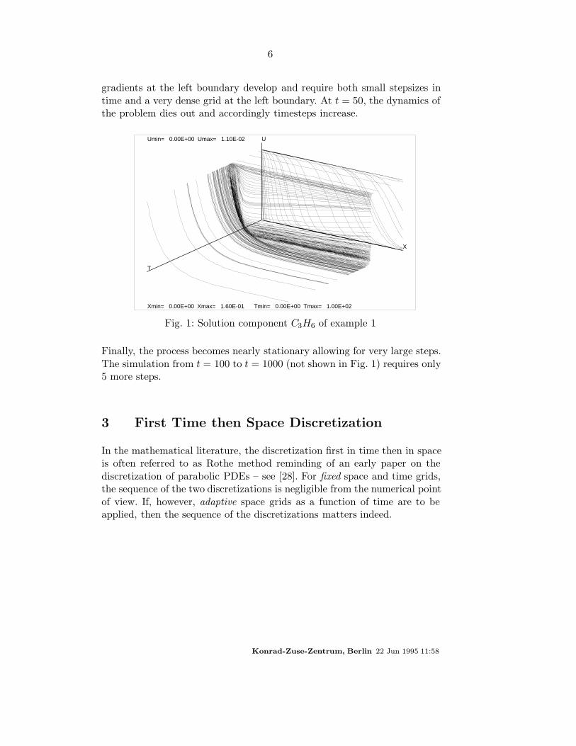
In order to reduce air pollution the study of the startup phase is of greatimportance. The simulation presented in [22] assumes that the polluted airenters with a linearly increasing temperature (and with constant velocity)at the left boundary. In Fig. 1 the concentration of the pollutant C3H6

is shown in a (x, t)–plane. The numerical solution on the computationalgrid is plotted at all internally selected integration points – as obtained bythe program PDEX1M. The displayed time interval is [0, 100] (whereas theactual integration interval was [0, 1000]).

Initially the converter is rapidly filled with inflowing gas. This shows upin Fig. 1 for small times (t ∈ [0, 0.2]) as a front moving from left to right. Inorder to resolve this fast process, small timesteps and a grid with local refi-nements within the front arise automatically. After the initial filling processis completed, the temperature is not yet high enough to start the reactionso that larger time steps and a coarser grid appear to be appropriate. Att = 25, the reaction starts and reduces the concentration of C3H6. Steep


6

gradients at the left boundary develop and require both small stepsizes intime and a very dense grid at the left boundary. At t = 50, the dynamics ofthe problem dies out and accordingly timesteps increase.

Umin= 0.00E+00 Umax= 1.10E-02

Xmin= 0.00E+00 Xmax= 1.60E-01 Tmin= 0.00E+00 Tmax= 1.00E+02

X

U

T

Fig. 1: Solution component C3H6 of example 1

Finally, the process becomes nearly stationary allowing for very large steps.The simulation from t = 100 to t = 1000 (not shown in Fig. 1) requires only5 more steps.

3 First Time then Space Discretization

In the mathematical literature, the discretization first in time then in spaceis often referred to as Rothe method reminding of an early paper on thediscretization of parabolic PDEs – see [28]. For fixed space and time grids,the sequence of the two discretizations is negligible from the numerical pointof view. If, however, adaptive space grids as a function of time are to beapplied, then the sequence of the discretizations matters indeed.


7

Adaptive Rothe Method. In his work on adaptive FEMs for parabo-lic PDEs, Bornemann[2, 3] introduced an algorithmic approach which isnowadays denoted by the term ”adaptive Rothe method”. For ease of pre-sentation, we start with the simple scalar parabolic equation

ut = (D(x)ux)x, u(x, 0) = u0(x) , boundary conditions . (5)

If we incorporate the boundary conditions together with the diffusion opera-tor into the operator A, then we may write (5) as an ODE in Hilbert spaceof the form

U ′ = AU, U(0) = U0. (6)

In this formulation, we may apply all the well-developed ODE technologyto solve this equation. For example, if we discretize this equation by theimplicit Euler method, we arrive at

(I − τA)ΔU = τAU0, U1 = U0 +ΔU. (7)

This is a special linear elliptic boundary value problem, which may be at-tacked by a FEM or FDM, where the FEM should be preferred, if thegeometry of the problem is sufficiently complicated. Extensions to higherorder time discretizations lead to one linear BVP per stage. Error estimatesrequired for the order and stepsize control may be approximated in the sameframework. In his first paper, which dealt with 1D problems only, Borne-mann had still used extrapolation methods, whereas in later papers, whichincluded 2D and 3D as well, he had designed a more sophisticated time dis-cretization of a recursive SDIRK type. In this approach higher order resultsUj are computed from corrections ηj via a multiplicative error correctionscheme of the form

Given u0, η0.

Compute for j = 1, . . . (8)

Uj+1 = Uj + ηj, ηj+1 = Rj(τA) ηj,

wherein the rational functions Rj satisfy Rj(∞) ≤ 1. (The whole time dis-cretization has the property R(∞) = 0 and is also applicable to degenerateparabolic equations.) As seen above, the corrections are computed in a mul-tiplicative way rather than in an additive way – so that small numbers are


8

computed by division rather than by subtraction. As a consequence, muchless stringent spatial error requirements compared with time errors are pos-sible as compared with extrapolation methods. Moreover, this variable ordertime discretization works on just one single space grid.

In Lang/Walter[16], the adaptive Rothe method has been carried overto the situation of reaction–diffusion systems (1). Proceeding as in the simpleparabolic case, we now arrive at an abstract ODE of the kind

U ′ = AU + F (U), U(0) = U0. (9)

with F representing the nonlinear reaction terms. One extension of the aboveimplicit Euler discretization for the linear parabolic equation is the linearly-implicit Euler method applied to the equivalent formulation

U ′ − AU − FU(U0)U = F (U)− FU(U0)U, U(0) = U0, (10)

which leads to

(I − τ(A+ FU (U0)))ΔU = τ(F (U0) + AU0), U1 = U0 +ΔU. (11)

This is a non–selfadjoint linear elliptic boundary value problem. As high-er order extension, Lang[17, 18] selected a linearly–implicit differential-algebraic method due to Roche [27], which has only 3 stages for order 3with embedded order 2 for stepsize control. As in the parabolic descendant,the discretization has R(∞) = 0 and requires only one spatial mesh. Themultiplicative error correction structure from above is not explicitly butessentially inherited. The method is of Rosenbrock type, which means thatit would require an exact representation of the operator A+FU (U0) – which,however, is not available in the FE context here. The thus unavoidableJacobian approximation errors may lead to restrictions of the time stepsobtained from the stepsize control – an effect, which has been observedexperimentally for low accuracy requirements. In principle, so–called W -methods (cf. the textbooks [15, 29, 8]) would be preferable to reflect theapproximation property of the problem correctly, which, however, wouldrequire more stages.


9

Cascadic Finite Element Methods. Up to now, we did not specifythe actual solution of the linear boundary value problems of the type (7)or (11). In both cases, an adaptive multilevel FEM has been applied. Weexplain the basic algorithmic approach for the simpler selfadjoint case first.In this case, the so-called cascade principle as developed by Deuflhard,Leinen, Yserentant[10] has been used. It starts with the direct solutionof the linear system obtained by the FE discretization on a comparativelycoarse grid, which, however, is assumed to catch the essential features ofthe problem formulation (boundary and interface conditions). The obtai-ned coarse grid solution is checked via FE error estimators in terms of theuser required accuracy. If this requirement is not yet met, then local errorindicators are used to obtain some refined grid. On the finer grid, the (in-terpolated) previous solution is used as starting point for a preconditionedconjugate gradient (PCG) iteration. This PCG iteration is terminated, assoon as an estimated algebraic error is sufficiently below the expected dis-cretization error, so as to avoid unnecessarily accurate computations on therefinement levels. After termination of the PCG iteration, the FE error esti-mator is once more applied to check for the user prescribed tolerance – to berepeated recursively until this tolerance is met on some finest mesh, whichin this way may come out to be highly non-uniform. As a preconditioner,the hierarchical basis preconditioner of Yserentant[32] may be used in2D, which has nearly optimal formal computational complexity and is quitecheap to implement. In 3D, the more costly so-called BPX preconditionerof Xu[5, 31] pays off, which has formally optimal computational complexity.Rather recently, even more effective so-called CCG methods have been de-veloped in Deuflhard[7] and Bornemann/Deuflhard[4], which avoidpreconditioning at all (apart from diagonal scaling) at the expense of a fewmore iterations on coarser grids, which are carefully controlled.

For the non–selfadjoint case of dynamical process simulation, the PCGiteration needs to be replaced by some unsymmetric iterative solver. Exten-sive numerical experiments clearly suggested the option BICG-STAB due to[30] in combination with SSOR preconditioning. In all the examples testedso far, this combination led to a nearly constant small number of iterati-ons on all refinement levels. So, even in this non–selfadjoint case, optimalcomputational complexity is achieved – however, without any theoretical ex-planation yet. As for the FE estimator to monitor the discretization errors,the present version of the program


10

Fig. 2: Nodal flux of Example 2 from method of lines treatment (above)versus Rothe method (below).


11

KARDOS (mnemotechnically for KAskade Reaction DiffusiOn System) rea-lizes a special interpolation error estimate – see [18].

Example 2: Comparative test problem [24].This 1D problem describesa moving flame front, which changes its shape during the process. In thepresent context, this example is just taken to illustrate the two differentadaptivity concepts described so far. In Fig. 2 the nodal flux (horizontal axis:space grids, vertical axis: time) obtained from the fully adaptive method oflines with static rezoning (above) is compared with the one obtained fromthe adaptive Rothe method with linear finite elements (below). Obviously,the plot below is a bit ”smoother” than the plot above, requiring less spatialnodes but more time steps – an observation, which nicely goes with theunderlying algorithmic concepts. In total, however, both pictures show astriking similarity. A comparison of the associated computing times, eventhough certainly desirable, is hard to give – at present, the two codes arejust too different. On the other hand, the example is just 1D and thereforenot at the center of interest of the present article.

Example 3: Thermally anchored flame [1]. This problem describesthe propagation of a two–dimensional premixed flame in a gaseous mix-ture. For the numerical simulation the adaptive Rothe method (programKARDOS) has been applied. Some simplifications of the underlying physi-cal processes lead to the so–called thermodiffusive model described by thereaction–diffusion equations

∂tT −�T = R(T, Y ) + V ∂xT

∂tY − 1

Le� Y = −R(T, Y ) + V ∂xY (12)

R(T, Y ) =β2

2 LeY exp

[ −β(1 − T )

1− α(1− T )

]

where T is a normalized temperature variable, Y is the reduced mass frac-tion of the reactant. The initial data are chosen to represent a planar steadyflame in the limit β → ∞. Furthermore, homogeneous Neumann conditi-ons are imposed at the whole tube wall except at some special part, wherethe temperature is forced to be equal to the adiabatic flame temperatureTA = 1. This additional condition inhibits the run-off of the flame throughthe reactor thus representing some thermal ”anchoring”. The problem wassolved for the parameters Le = 1, β = 10, α = 0.84, V = −5.

A correct simulation of the flame propagation requires a dense computa-tional mesh within the thin flame region, and especially in the boundarylayer caused by the time–fixed Dirichlet condition. First experiences have


12

Fig. 3: Adaptive grids at t=0.0, 2100 nodes (above); t=1.35, 2900 nodes(middle); at t=4.29, 14000 nodes (below)

shown that at least a tolerance TOL = 1.0e− 4 is needed to reflect the dy-namics of the process adequately. Such a quite stringent tolerance requires2100 nodes at the beginning up to 14000 nodes at the end of the process.Note, however, that estimated 1010 triangles would be needed to guaranteethe same accuracy on a uniform mesh. In Fig. 3 the dynamics of the griddevelopment is shown, whereas in Fig. 4 the level surfaces of the solutionare given for comparison. The whole computation is rather time consuming;speed-ups would certainly be possible replacing the linear finite elements bysome h− p−strategy [33] for higher order elements – which is the subject offurther work.


13

Fig. 4: Adaptive solutions at t=0.0 (above), t=1.35 (middle), t=4.29 (below)

Conclusion

Dynamical simulation of industrially relevant processes strongly advises theuse of algorithms, which are adaptive both in time and in space discretiza-tion. The paper presented two alternatives: (a) a fully adaptive method oflines approach, which is based on finite difference methods and essentiallyapplicable to 1D problems; (b) a fully adaptive Rothe method, which is ba-sed on a fast multilevel finite element method and applicable to 1D up to3D.


14

Bibliography

[1] F. Benkhaldoun, B. Larrouturou: Explicit adaptive calculations of wrinkledflame propagation. Int. J. Numer. Meth. in Fluids 7, p. 1147–1158 (1987)

[2] F.A. Bornemann: An Adaptive Multilevel Approach to Parabolic Equations.I: General Theory and 1D–Implementation. IMPACT Comput. Sci. Engrg. 2,p. 279–317 (1990)

[3] F.A. Bornemann: An Adaptive Multilevel Approach to Parabolic Equations. II:Variable Order Time Discretization Based on Multiplicative Error Correction.IMPACT Comput. Sci. Engrg. 3, p. 93–122 (1991)

[4] F. Bornemann, P. Deuflhard: Cascadic multigrid methods for elliptic problems.Submitted to Numer. Math. (1994)

[5] J.H. Bramble, J.E. Pasciak, J. Xu: Convergence estimate for multigrid algo-rithms without regularity assumptions. Mat. Comp. 57, p. 23–45 (1991)

[6] P. Deuflhard: Recent Progress in Extrapolation Methods for ODE’s. SIAMReview 27, p. 505–535 (1985)

[7] P. Deuflhard: Cascadic conjugate gradient methods for elliptic partial diffe-rential equations: algorithm and numerical results. D.E Keyes, J. Xu (eds.):AMS, Contemporary Mathematics Vol. 180, p. 29–42 (1994)

[8] P. Deuflhard, F. Bornemann: Numerische Mathematik II. – Integration vongewohnlichen Differentialgleichungen. de Gruyter Lehrbuch, Berlin, New York(1991)

[9] P. Deuflhard, U. Nowak: Extrapolation Integrators for Quasilinear ImplicitODE’s. In: P. Deuflhard, B. Engquist (eds.): Large Scale Scientific Computing.Progress in Scientific Computing, Birkhaeuser 7, p. 37–50 (1987)

[10] P. Deuflhard, P. Leinen, H. Yserentant: Concepts of an Adaptive HierarchicalFinite Element Code. IMPACT Comput. Sci. Engrg. 1, p. 3–35 (1989)

[11] P. Deuflhard, U. Nowak, M. Wulkow: Recent Developments in Chemical Com-puting. Computers Chem. Engrg. 14, p. 1249–1258 (1990)

[12] J.E. Flaherty, P.K. Moore, C. Ozturan: Adaptive Overlapping Grid Methodsfor Parabolic Systems. In: J.E. Flaherty, P.J. Paslow, M.S. Shephard, J.D. Va-silakis (eds.): Adaptive Methods for Partial Differential Equations, SIAM ,p. 176–193 (1989)

[13] F.N. Fritsch, J. Butland: AMethod for Constructing Local Monotone PiecewiseCubic Interpolants. SIAM J. Sci. Stat. Comput. 5, p. 300–304 (1984)


15

[14] C.W. Gear: Numerical Initial Value Problems in Ordinary Differential Equa-tions. Prentice Hall (1971)

[15] E. Hairer, G. Wanner: Solving Ordinary Differential Equations II. – Stiff andDifferential–Algebraic Problems. Springer Series in Computational Mathema-tics 14, Springer Verlag, Berlin–Heidelberg (1991)

[16] J. Lang, A. Walter: A finite element method adaptive in space and time fornonlinear reaction–diffusion systems. IMPACT Comput. Sci. Engrg. 4, p. 269–314 (1992)

[17] J. Lang: High–resolution selfadaptive computations on chemical reaction–diffusion problems with internal boundaries. Submitted to Chem. Engrg. Sci.

[18] J. Lang: Two–dimensional fully adaptive solutions of reaction–diffusion equa-tions. Accepted for publication in Appl. Numer. Math. (1995)

[19] U. Maas, J. Warnatz: Simulation of chemically reacting Flows in two–dimensional geometries. IMPACT Comput. Sci. Engrg. 1, p. 394–420 (1989)

[20] P.K. Moore, J.E. Flaherty: High–order adaptive finite element–singly implicitRunge–Kutta methods for parabolic differential equations. BIT 33, p. 309–331(1993)

[21] U. Nowak: Adaptive Linienmethoden fur nichtlineare parabolische Systeme ineiner Raumdimension. Technical Report TR 93–14, Konrad–Zuse–ZentrumBerlin (1993)

[22] U. Nowak, J. Frauhammer, U. Nieken, G. Eigenberger: A fully adaptive al-gorithm for parabolic partial differential equations in one space dimension.accepted for publication in Comput. & Chem. Engrg. (1995)

[23] A.C. Hindmarsh: ODEPACK, A Systematized Collection of ODE Solvers. InScientific Computing, R. S. Stepleman et al. (eds.), North–Holland, Amster-dam, p. 55–64 (1983)

[24] N. Peters, J. Warnatz (Eds): Numerical Methods in Laminar Flame Propaga-tion. Notes in Numerical Fluid Dynamics 6, p. 232–260, Vieweg (1982)

[25] L.R. Petzold: A Description of DASSL: a differential–algebraic system solver.Proc. IMACS World Congress, Montreal, Canada (1982)

[26] L.R. Petzold: An adaptive Moving Grid Method for One–Dimensional Systemsof Partial Differential Equations and its Numerical Solution. Proc. Workshopon Adaptive Methods for Partial Differential Equations, Renselaer PolytechnicInstitute (1988)


16

[27] M. Roche: Rosenbrock methods for differential algebraic equations. Numer.Mat. 52, p. 45–63 (1988)

[28] E. Rothe: Zweidimensionale parabolische Randwertaufgaben als Grenzfall ein-dimensionaler Anwendungen. Math. Ann. 102, p. 650–670 (1930)

[29] K. Strehmel, R. Weiner: Linear–implizite Runge–Kutta–Methoden und ihreAnwendung. Teubner–Texte zur Mathematik, Band 127, B.G. Teubner Ver-lagsgesellschaft, Stuttgart–Leipzig (1992)

[30] H.A. van der Vorst: BI–CGSTAB: A fast and smoothly converging variant ofBI–CG for the solution of nonsymmetric linear systems. SIAM J. Sci. Stat.Comp. 13, No. 2, p. 631–644 (1992)

[31] J. Xu: Theory of Multilevel Methods. Department of Mathematics, Pennsyl-vania State University, University Park, Report No. AM 48, Thesis (1989)

[32] H. Yserentant: On the multilevel splitting of finite element spaces. Numer.Math. 49, p. 379–412 (1986)

[33] G.W. Zumbusch: Simultanous h-p Adaptation in Multilevel Finite Elements,Freie Universitat Berlin, Fachbereich Mathematik, Thesis (1995)


adaptive algorithms in dynamical process simulation … · 1 adaptive algorithms in dynamical...

Documents