Sick of the Welfare State? Adaptation in theDemand for Social Insurance

Martin Ljunge∗

University of Copenhagen and SITE

November 22, 2010

Abstract

We argue that the supply of social insurance programs has long termeffects on individual demand for program benefits. We postulate a modelwhere the utility of taking up social insurance benefits depends on oldergenerations’ past behavior, and we estimate the model using individualpanel data. This intertemporal mechanism can account for three-quartersof the younger generations’ higher demand for social insurance benefits.The influence of older generations’ behavior remains when we instrumentusing mortality rates.

JEL codes: H31, I18, J22, Z13Key words : social insurance, adaptation, norm dynamics, role models

1 Introduction

We study the dynamic adaptation of behavior in the welfare state. We find

substantial long run adaptation with regard to demand for welfare state ben-

efits. More specifically, we find an almost 1 percentage point increase in the

benefit take up per birth cohort. We estimate a structural model that allows

for preferences to adapt to aggregate behavior, in effect allowing social norms

to adjust to observed behavior. The dynamic model we estimate differs from

the previous cultural transmission literature that has focused on determinants

of different equilibria, but largely ignored the analysis of the path towards a

∗University of Copenhagen, Department of Economics, Øster Farimagsgade 5, building26, 1353 København K, Denmark, martin.ljunge@econ.ku.dk. I’d like to thank James Heck-man, Austan Goolsbee, Bruce D. Meyer, Casey B. Mulligan, Marianne Bertrand, Søren Leth-Petersen, Sten Nyberg, and Kelly Ragan for valuable discussions and suggestions. I acknowl-edge support from the Riksbank Tercentiary Foundation, grant P2007-0468:1-E.

1

new equilibrium.1 We study the adaptation process following the expansion of

welfare state institutions, and estimate the speed at which rational agents adapt

to the social conditions in a simple structural model used by theorists.2.4

.5.6

.7.8

Par

ticip

atio

n R

ate

1920 1930 1940 1950 1960Year of birth

Sample: Labor force participants, ages 22-60. Years 1974-1990.

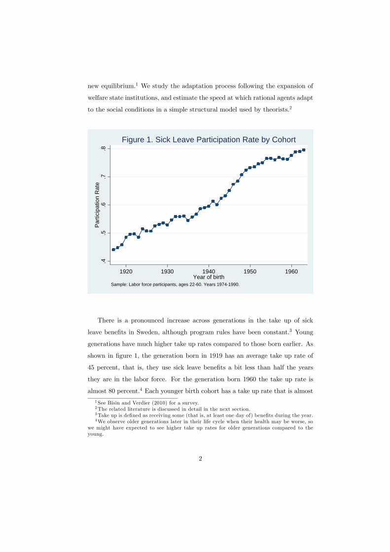
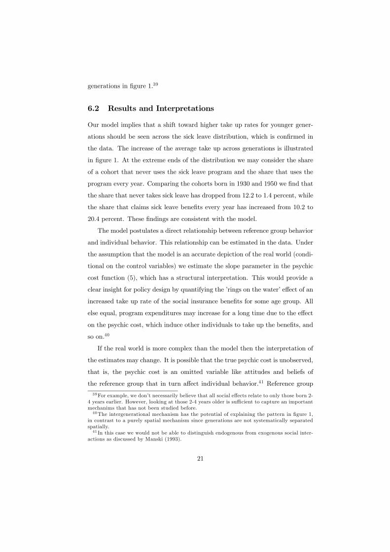
Figure 1. Sick Leave Participation Rate by Cohort

There is a pronounced increase across generations in the take up of sick

leave benefits in Sweden, although program rules have been constant.3 Young

generations have much higher take up rates compared to those born earlier. As

shown in figure 1, the generation born in 1919 has an average take up rate of

45 percent, that is, they use sick leave benefits a bit less than half the years

they are in the labor force. For the generation born 1960 the take up rate is

almost 80 percent.4 Each younger birth cohort has a take up rate that is almost

1See Bisin and Verdier (2010) for a survey.2The related literature is discussed in detail in the next section.3Take up is defined as receiving some (that is, at least one day of) benefits during the year.4We observe older generations later in their life cycle when their health may be worse, so

we might have expected to see higher take up rates for older generations compared to theyoung.

2

1 percentage point higher than those born one year earlier. We account for

a large number of factors that could influence benefit take up and potentially

explain the cohort trend. Yet, this trend persists.

Our analysis contributes to a primarily theoretical literature on long term

dynamics. Our model builds most closely on Lindbeck, Nyberg, and Weibull

(1999, 2003), but it is also closely related to the evolution of work norms mod-

eled in Doepke and Zilibotti (2008) as well as the dynamics of the welfare state

in Hassler, Mora, Storesletten, and Zilibotti (2003). While theorists have hy-

pothesized about changes in work norms in the welfare state, the aggregate

data we present suggests that behavior has adapted significantly in the face of

constant institutions. Quantifying the size of this adjustment and estimating a

particular mechanism through which this adjustment takes place is an empirical

question that to our knowledge we are the first to provide an answer to.

The social interactions literature is different as it usually assumes an imme-

diate adaptation to some social influence, or as in the studies of the long term

effects of institutions, that the adaptation process has reached a new stationary

equilibrium. The argument is that different social conditions, either contem-

poraneous or historical, have resulted in different stationary equilibria across

different locations, but how these equilibria are reached is a black box. We are

different in that we study the adaptation process before it reaches a station-

ary state. Our analysis is fundamentally distinct from the social interactions

literature and from studies of the persistent effects of institutions in that both

literatures are based on cross-sectional differences.5 We study intertemporal dif-

ferences, across generations and within life cycles, to examine how individuals

adapt to social conditions.

The psychic cost we model, which operates on the demand for benefits, would

apply to any social insurance program.6 We focus on the take up of sick leave

5Studies of the influence of culture using immigrants, as surveyed in Fernandez (2010),have a similar focus on cross-sectional differences.

6We use the word psychic cost to describe the mechanism. What we model and estimate isthe influence of reference group behavior. This may be, internal or external, stigma or someother effect that is captured by the reference group’s behavior.

3

benefits in Sweden. What makes the program particularly suited for study

is the lack of supply side constraints. Behavior reveals demand without any

supply interference, as claiming some benefits is completely at the individual’s

discretion.

We write down an empirical model of program participation that includes

a psychic cost for claiming benefits, based on Lindbeck, Nyberg, and Weibull

(2003). We estimate a psychic cost function and quantify how older cohorts’

past behavior influences individual behavior. The estimated model can account

for three-quarters of the increased demand across generations.

We estimate the importance of the psychic cost versus a general shift over

time towards more social insurance take up. We are also able to quantify the

importance of factors that are constant within an individual versus the impor-

tance of the psychic cost that varies over time. This provides a quantification of

the relative importance of time varying social influences compared to culture.

Culture is considered the slow moving part of preferences,7 for example the work

norms instilled by your parents.

We apply an instrumental variables approach to identify the intertemporal

influence of older cohorts. We use mortality rates as an instrument for the older

cohorts’ sick leave behavior. This approach isolates the influence of the older

generations’ behavior to the part that is shifted by the mortality shocks, and

the estimator isn’t affected by fixed factors like culture. The influence of the

older cohorts’ behavior remains strong.

The paper is organized as follows. The next section discusses the related

literature. The third section describes the sick leave program, followed by the

data description. Section 5 examines the cohort trend by accounting for indi-

vidual characteristics. In the sixth section we develop our empirical model and

we present the empirical results. Section 7 concludes.

7This distinction between time varying social influence and culture is discussed in Guiso,Sapienza, and Zingales (2006).

4

2 Related Literature

Our study of long term adjustments in demand for social insurance, where we

follow individual behavior across decades, complements several existing litera-

tures. The effect of norms on labor supply (or benefit up take) has been studied

both theoretically and empirically. Our model is most closely related to Lind-

beck, Nyberg, and Weibull (2003) in how we model individual heterogeneity and

the psychic cost, but it is also close to Lindbeck, Nyberg, and Weibull (1999).

Other models with delayed responses are the intergenerational transmission of

traits or work norms by Doepke and Zilibotti (2008), Bisin and Verdier (2001),

Lindbeck and Nyberg (2006), and Tabellini (2008). We examine the influence

of role models across generations rather than the link between parents and chil-

dren. Empirical applications include transmission of work norms from parents

to children (Fernandez, Fogli, and Olivetti, 2004; Lindbeck and Nyberg, 2006)

and the transmission of religious beliefs (Bisin, Topa, and Verdier, 2004; Bisin

and Verdier, 2000).

There is a growing literature on the impact of beliefs or culture on eco-

nomic outcomes8 and our paper is closely related to studies of how institutions

and policy interact with beliefs. Our question is similar to studies on how

institutional arrangements affect norms, like the effect of Communism on at-

titudes towards redistribution studied in Alesina and Fuchs-Schündeln (2007).

They study the effects of the social system on self reported preferences while

we study behavior. Another example is the effect of minimum wage on norms

regarding cooperation in the labor market as examined in Aghion, Algan, and

Cahuc (2008). We study how exposure to welfare state programs affects demand

for social insurance, where demand may be affected by norms with respect to

claiming government benefits.9 , 10 Changes in such norms may affect the social

capital in society and economic outcomes. Aghion, Algan, Cahuc, and Shleifer

8See the handbook edited by Benhabib, Jackson, and Bisin (2010).9Our mechanism is similar to what Beaman, Chattopadhyay, Duflo, Pande, and Topalova

(2009) explore in the sense that exposure affects preferences, which in turn affect actions.10A related mechanism is social learning as studied by Fernandez (2008).

5

(2010) argue that social capital in the form of trust affects regulation, based on

a cross-country analysis. Algan and Cahuc (2010) use a model of intergenera-

tional transmission of beliefs to examine the effect of trust on per capita income.

Our study complements this literature by studying dynamics of norms within

one country. Individual panel data allow us a much richer analysis with respect

to the intertemporal adaptation and more detailed sets of controls, including

fixed individual characteristics, where the related literature to a large extent

rely on country level variation.

Social interactions is a related literature, but distinct from our intertemporal

analysis as discussed above. That literature focuses on cross-sectional or spatial

mechanisms, for example a contemporaneous effect of benefit up take in your

reference group on your behavior. The effects of social interactions in the take

up of welfare benefits have been studied empirically by Bertrand, Luttmer, and

Mullainathan (2000) and Edin, Fredriksson, and Åslund (2003).11 The effects

of social norms have been studied in the context of unemployment insurance, a

related social insurance program, see Bruegger, Lalive, and Zweimueller (2010),

Stutzer and Lalive (2004), and Clark (2003). None of these studies of social

interactions have analyzed the intertemporal adaptation process, which we do.

The program participation literature casts the take up decision as a trade

off between time and consumption. Another way to view the sick leave de-

cision is as an expression of well-being, which ties in to the literature on self

reported well-being.12 What we have labelled a psychic cost may be seen as a

relative or positional concern in the language of the well-being literature. This

literature builds on a model where the relative position has a contemporane-

ous effect on well-being, for example Luttmer (2005) finds that individuals who

have neighbors with higher income have lower well-being, while controlling for

11Two papers on the social interactions in the use of sick leave in Sweden are Hesselius,Johansson, and Vikström (2009) and Lindbeck, Palme, and Persson (2008). Both papers focuson contemporaneous spatial interactions. Henrekson and Persson (2004) studies sick leave inSweden in a long time series.12Graham (2009) finds that health is the strongest correlate with self reported well-being in

a large cross section of countries. Daly and Wilson (2009) study suicides as a manifestationof low subjective well-being, which is similar to our argument regarding sick leave.

6

own income and characteristics as well as neighborhood factors.13 , 14 That is,

they assume an immediate cross-sectional, usually spatial, effect of the refer-

ence group’s income/consumption on your well-being. Our model focuses on

an intergenerational link the existing empirical literature has not entertained.

Furthermore, all these papers use self-reported survey measures of well-being,

which has short comings as discussed by Bertrand and Mullainathan (2001) and

Ravallion and Lokshin (2001). Our measure of well-being, sick leave, is based

on actions, which we think overcome shortcomings of the previous literature.

Our paper is also related to the literature on the intergenerational trans-

mission of economic status, for example father and son earnings correlations as

studied in Mulligan (1997) and surveyed in Solon (2002). There are also stud-

ies of intergenerational links in welfare take up, Solon, Corcoran, Gordon, and

Laren (1988) and Beaulieu, Duclos, Fortin, and Rouleau (2005).15 That litera-

ture focuses on mechanisms within the family, which probably are relevant in

our setting as discussed later. However, we allow for broader influences across

time and generations that are not limited to family influences.

3 The Sick Leave Program

Sweden has a generous publicly run sick leave insurance program that covers

lost earnings in the case of basically any injury or illness.16 It is very easy to

claim the benefits. For the first week of each spell, the law gives the individual

13Additional evidence that well-being is partly driven by relative position are Van de Stadt,Kapteyn, and Van de Geer (1985), Clark and Oswald (1996), Blanchflower and Oswald (2004),Ferrer-i-Carbonell (2005), Graham and Felton (2006), Kingdon and Knight (2007), and Clark,Kristensen, and Westergård-Nielsen (2008). Dynan and Ravina (2007) find evidence thatrelative concerns exist in some domains (like consumption of private goods) but not in others(like leisure and public goods such as defense).14 Individual concerns of relative income and consumption and their implications for both

taxes and public expenditures have been studied theoretically by Boskin and Sheshinski (1978),Layard (1980), Oswald (1983), Ng (1987), Seidman (1987), Ireland (1998), Ljungqvist and Uh-lig (2000), Dupor and Liu (2003), and Abel (2005). Quantifying these relative considerationsis an empirical question, where our study makes a contribution.15Oreopoulos, Page, and Stevens (2008) study the effect of parental job loss on children’s

adult income and program participation.16 In a comparison to the U.S. the program encompasses both ’personal days’ provided

in employment contracts (although restricted to sick leave) and the workers’ compensationprogram.

7

the discretion to determine if he is fit to work or not. If he wants to claim the

sick leave benefits he makes two phone calls, one to the social insurance office

and one to his employer.17 There is no fixed allocation of sick leave days, you

can use the insurance as long as your sickness requires and for as many spells

as you like. For spells up to 7 days the individual himself determines if he is fit

to work. For spells longer than 7 days it is required that a physician validates

your condition.18 Monitoring of actual sickness is very light, at least in part

due to the difficulty in verifying conditions like stomach ache and back pain.

The program is similar to any social insurance. It pays out benefits if the

individual is hit by some shock. In the sick leave program it is a health shock,

while unemployment benefits cover unemployment shocks and pensions pay out

based on age. What sets the sick leave program apart is the level of individual

discretion with respect to claiming benefits. The decision to claim benefits rests

entirely with the individual, and observed take up behavior is purely driven by

the demand for benefits.

The rules governing sick leave insurance have been remarkably constant over

the 1974-1990 period. The sick leave program was first passed into law in 1962

(SFS 1962:381) and it took effect in 1963. Data on sick leave are available from

1974, when sick leave benefits became taxable income19. The replacement rate

for lost earnings due to sickness was set to 90 percent. The daily benefit is

calculated as 90 percent of normal annual labor earnings divided by 365, up to

a cap. The replacement cap is indexed to the so called base amount, which is

related to inflation. About 93 percent of the incomes are below the cap, and 6

percent of the sick leave observations are above the cap.

Benefits can be claimed from the second day of the sickness spell. The

definition of the second day is, however, quite generous. It is sufficient to call

in sick before leaving work and that day counts as the first day of the spell.

If you think you’ll be sick tomorrow you can always call in sick today and the

17Benefits are paid by the social insurance office directly to the claimant.18 Since we analyze the extensive margin, the validation by the physician is not relevant in

our study.19The updates to the program are detailed in law SFS 1973:465.

8

first unpaid day is of no consequence, and if it turns out that you’re fit for work

tomorrow you can change your mind. Spells shorter than 7 days do not pay

benefits on weekends. This system was in place until 1987. From 1988 through

1990 the first day of no coverage was abolished.20 , 21

Most sick leave spells are short, about 95 percent are shorter than one month

(Source: Försäkringskassan). You need to have earnings for six months in order

to qualify for the sick leave benefits and be less than 65 years of age. The

program is universal and it is administered by the central government and does

not depend on your employer. Benefits are financed through a flat pay roll tax.

4 Data

We use registry data on individual panels over the period 1974 to 1990 (from

1973 for lagged income).22The data draw information from several sources; de-

mographic information from the population registry, income information from

the tax authorities, and various public benefits from the social insurance admin-

istration. Our main dependent variable, participation in the sick leave programs,

is defined based on observing positive sick leave benefits during the year. We

use a random sample of the 1974 population who we follow for 17 years.23 We

include the birth cohorts from 1917 to 1963. About 3 percent of the population

is sampled. In addition, household members are included in the data. This

allows us to control for the household composition as well as spousal income.

20The updates to the program are detailed in law SFS 1987:223.21Reforms in the 1990’s make the later data hard to compare to the period we study.22The analysis ends in 1990 since later reforms make the data hard to compare.23The only sampled individuals that disappear from the data are those who die or emigrate.

9

Table 1. Summary statistics.

Mean Std. Dev. Min Max Obs.Sick leave participation 0.637 0.481 0 1 1930462Year of birth 41.9 11.3 17 63 1930462Earned income, lagged 127519 319262 0 1.99E+08 1929137Capital income, lagged 1748 57136 0 4.81E+07 1929137Age 40.0 10.7 22 60 1930462Man 0.525 0.499 0 1 1930462College, 3+ years 0.113 0.316 0 1 1930462< 3 years college 0.091 0.287 0 1 1930462High school 0.380 0.485 0 1 1930462Married 0.602 0.490 0 1 1930462Months with infant x Woman 0.101 0.757 0 7 1930462Children aged 7 months to 2 years 0.064 0.249 0 4 1930462Children aged 3 to 6 years 0.131 0.341 0 3 1930462Children aged 7 to 15 years 0.286 0.460 0 3 1930462Husband's income, lagged 56178 288605 0 1.68E+08 1929137Wife's income, lagged 26976 57974 0 2.10E+07 1929137Employment rate, by county 0.870 0.021 0.807 0.912 1930462Average earnings, by county 130946 14071 94790 173337 1930462Sample: Labor force participants, 22-60 years old. Amounts in 1990 SEK.

Individuals are included in the analysis from ages 22 to 60. The age restric-

tions are due to the looser connection to the labor market of individuals at the

tails of the life cycle. The young may still be studying and may not have a firm

foot in the labor market. At ages close to retirement individuals face a number

of incentives to leave the labor force that we don’t model here, and we choose to

exclude those observations. Since the sick leave program is designed to replace

lost labor earnings, we restrict the analysis to individuals who are labor force

participants.24 Summary statistics are presented in table 1.

5 Increased Demand For Social Insurance

We account for a number of individual and aggregate factors that could explain

the behavioral differences across cohorts seen in figure 1. We also perform a

number of robustness checks, yet none of these specifications can account for

the pattern in figure 1. We allow for non-linearities in the cohort trend and

estimate the model separately for men and women, yet the trend persists.24Labor force participation is defined as having positive labor earnings during the year.

10

It is possible the raw averages in figure 1 capture life cycle patterns, for ex-

ample, young generations are observed when they have young children that may

make them take more sick leave during those years.25 In figure 2 we plot the

average take up by age for four different cohorts where we can compare cohorts

at the same stage in the life cycle. Men are plotted in the left panel and women

on the right. Across the entire life cycle, younger generations have higher take

up. The pattern is particularly pronounced for women.

.4.5

.6.7

.8.9

Parti

cipa

tion

Rat

e

20 30 40 50 60Age

Year of birth 1955 1945 1935 1925

Four Cohorts of Men from 1974 to 1990

.4.5

.6.7

.8.9

Parti

cipa

tion

Rat

e

20 30 40 50 60Age

Year of birth 1955 1945 1935 1925

Four Cohorts of Women from 1974 to 1990

Sample: Labor force participants, ages 22-60.

Figure 2. Sick Leave Participation for Men and Women.

We may be concerned that changes in labor force participation are behind

the increasing sick leave take up across generations. For women the labor force

participation rates have increased across generations and the 1955 cohort of

women have rates similar to men. Men’s labor force participation rates have

been constant across generations (along the life cycle paths), indicating that

labor force participation changes don’t explain the increased sick leave take up.

This issue is examined further below.25There are at least two causes for this. Parents may use the sick leave program to take

care of sick children, or sick children make the parents sick.

11

So far we have just looked at raw averages. Column 1 of table 2 gives us the

average slope of the cohort trend, 0.8 percentage point per year, which adds up

to a 16 points higher take up rate for a cohort born 20 years later than the base

cohort. The results are from using the between estimator, that is, we compare

the individual averages over time across individuals. Since the focus is on the

differences in behavior across cohorts we think it is the appropriate estimator.

Table 2. Cohort trend in sick leave program participation.

Dependent Variable: Indicator of Positive Sick LeaveBetween EstimatorVariable (1) (2) (3) (4) (5) (6)

Year of birth 0.0080 0.0098 0.0112 0.0110 0.0112 0.0067(.0001) (.0003) (.0003) (.0004) (.0004) (.0004)

Age, age sq interacted Yes Yes Yes Yes Yeswith gender and education

Months with Infant x Female Yes Yes Yes YesChild 7 months-2 years Yes Yes Yes YesChild 3-6, Child 7-15 years Yes Yes Yes YesMarital status Yes Yes Yes Yes

Income lag Yes YesCapital income lag Yes Yes YesSpouse's income lag Yes Yes Yes

Business cycle control Yes Yes YesRegional fixed effects Yes Yes Yes

Permanent income YesPermanent income spline YesIncome lag spline Yes

Observations 1955700 1930500 1930500 1929100 1929100 1929100Notes: Education is gouped into 3+ years of college, <3 years of college, high school, <high school.Months with infant counts the number of months there is a child of up to 7 months of age in the household.Business cycle control is average regional employment rates.Permanent income is an estimated individual fixed effect of earnings on demographic interactions and BC controls. Spline is 5 piece with knots at quintiles.Individual panel data from 1974-1990, annually. Estimates of the between estimator.Standard errors in parenthesis. Sample: Labor force participants, 22-60 years old.

One concern may be that the raw average is confounded by life cycle pat-

terns, which may vary by groups as seen in figure 2. We include a full set of

12

interactions between gender, the four education groups,26 age and age squared.

Including these controls raise the estimated cohort trend as seen in column 2. If

parents with young children take more sick leave, and these parents are mostly

observed among the younger cohorts, it may bias our estimate of the cohort

trend upwards. It may hence be important to have detailed controls of the

number of children at different ages. Such controls are included in column 3,

and the estimated cohort trend increases somewhat.

Younger cohorts tend to have higher education and may have higher earnings

(conditional on age) than older cohorts. If sick leave is one dimension of leisure

(a normal good), it may be that the higher take up rate is in part an income

effect. We control for own earnings and capital income as well as the spouse’s

income (if present). The income variables are lagged one year since current

income and sick leave take up may be jointly determined. We also control for

regional business cycles (through the regional employment rate) and regional

fixed effects.27 Including these controls do not affect the cohort trend, as seen

in column 4.

It is possible that not only current earnings but lifetime earnings affect the

sick leave choice. Using the panel data, we run an individual fixed effect (within)

regression of individual earnings on the age-gender-education interactions men-

tioned above and business cycle controls. The individual fixed effect from that

regression is our measure of permanent income, which we include in the regres-

sion in column 5. It does not have much of an impact on the cohort trend.

Linearity of the income effects may be a strong assumption that we relax in

column 6. We construct five piece splines of both permanent income and lagged

income. This allows the income effects to differ across quintiles both for perma-

nent and lagged income. This has a substantial impact on the estimated cohort

trend, which now is estimated at 0.67 percentage points. The specification in

column 6 will be the baseline in the analysis below.

Linearity of the cohort trend is assumed in table 2. We replace the linear26The four education groups are 3 or more years of college, less than 3 years of college, high

school degree, and less than a high school degree.27Our objective is not to explain regional differences in take up. There are 8 regions.

13

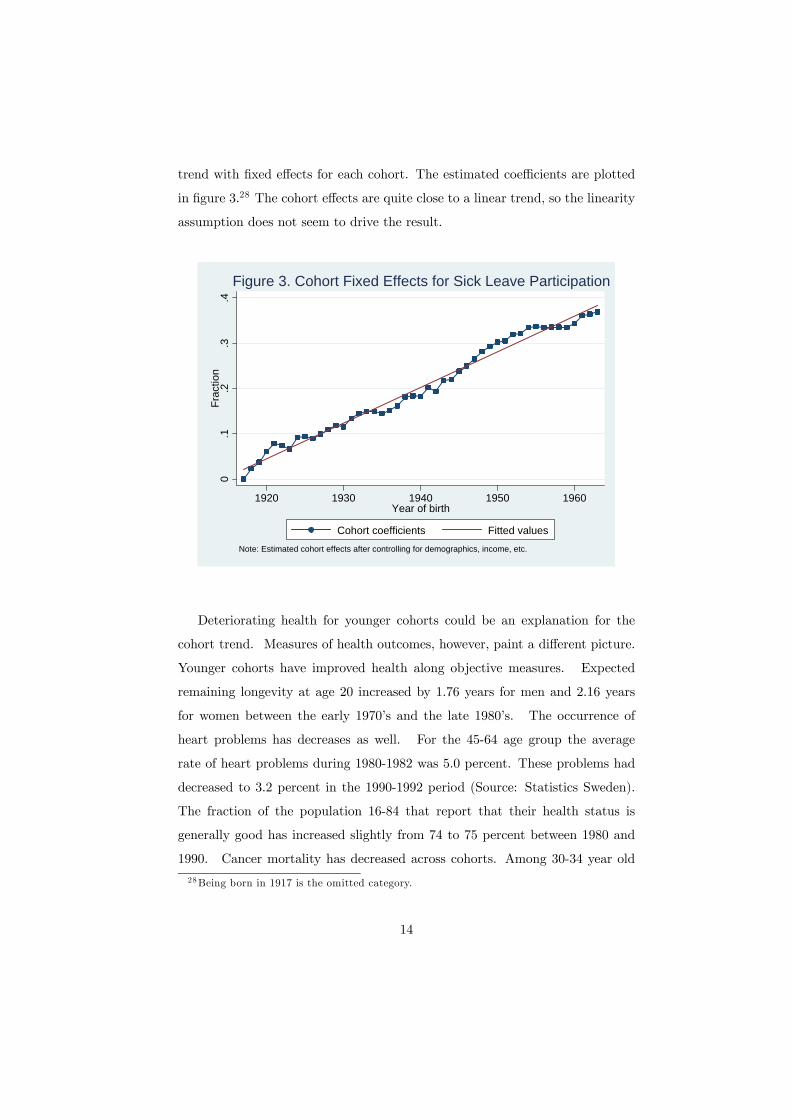
trend with fixed effects for each cohort. The estimated coefficients are plotted

in figure 3.28 The cohort effects are quite close to a linear trend, so the linearity

assumption does not seem to drive the result.0

.1.2

.3.4

Frac

tion

1920 1930 1940 1950 1960Year of birth

Cohort coefficients Fitted valuesNote: Estimated cohort effects after controlling for demographics, income, etc.

Figure 3. Cohort Fixed Effects for Sick Leave Participation

Deteriorating health for younger cohorts could be an explanation for the

cohort trend. Measures of health outcomes, however, paint a different picture.

Younger cohorts have improved health along objective measures. Expected

remaining longevity at age 20 increased by 1.76 years for men and 2.16 years

for women between the early 1970’s and the late 1980’s. The occurrence of

heart problems has decreases as well. For the 45-64 age group the average

rate of heart problems during 1980-1982 was 5.0 percent. These problems had

decreased to 3.2 percent in the 1990-1992 period (Source: Statistics Sweden).

The fraction of the population 16-84 that report that their health status is

generally good has increased slightly from 74 to 75 percent between 1980 and

1990. Cancer mortality has decreased across cohorts. Among 30-34 year old

28Being born in 1917 is the omitted category.

14

women in the late 1960’s the mortality of cancer was 21 per 100 000 persons.

In the early 1990’s the rate had dropped to 13.5. The corresponding rates for

men were 16.7 and 11.2. Reductions in mortality rates are seen at most points

in the age distribution across cohorts (Source: NORDCAN). Improvements in

health conditions across cohorts make the sick leave trends more surprising.

Even though we controlled for a host of factors above there may still be

alternative explanations to the trend. One concern may be the measurement

of sick leave benefits. Up until 1983 maternity leave was included in sick leave

benefits but starting in 1984 the parental leave in connection to the birth of

a child was reported separately. In addition, care for sick child was reported

separately from 1987. These definitional changes could affect the analysis. To

examine the impact we redefine the sick leave variable as take up of either of

the three programs (sick leave, parental leave, care for sick child). Redefining

the dependent variable does not affect the estimated cohort trend.29

Since sick leave is not the only program individuals may use it is possible

that there is some shifting across programs, which could influence our estimate.

To examine the sensitivity to the use of other programs we exclude individuals

who have taken up either unemployment benefits or welfare payments during

the year. The estimated cohort trend in specification 2 in table 3 is somewhat

lower with this sample restriction, indicating a stronger trend among individuals

that use other programs.30

The next two alternative specifications deal with the composition of the

labor force. Since the main regressions condition on being in the labor force

we may be concerned that individuals that have left the labor force would have

been on sick leave if the had remained in the labor force. In particular, we may

29 It’s possible that young children are not appropriately controlled for by the linear controls.To address this we exclude women with children between the ages 0 and 2 (only women sincecare of young children were mostly done by women during the period we study). Excludingthis group does not affect the cohort trend.30Employers do not seem to collude with young workers. During slow times there may be

an incentive for the employer to reduce cost by inducing employees to take sick leave (paid bythe government). Younger workers with less job protection may be more likely to enter intosuch an arrangement, which potentially could explain the cohort trend. We include sectorfixed effects interacted with an indicator if the person is less than 30 years old. It does nothave a large impact on the cohort trend.

15

be concerned that among the older people only the healthy remain in the labor

force, which could drive our finding. To address this we restrict the sample

to those between 22 and 45 years of age, where there is little exit from the

labor force. This restriction does not affect the cohort trend much as seen

in specification 3.31Another approach is to assume that everyone outside the

labor force would have been on sick leave had they been in the labor force. We

redefine sick leave such that all individuals outside the labor force are added

to the sick leave rolls (and we no longer condition on being in the labor force).

This extreme case provides a lower bound for the cohort trend. The estimated

trend is as expected lower, a little shy of half the magnitude, but still significant

as shown in column 4. Changes in labor force composition can’t explain the

cohort trend.

Table 3. Alternative explanations of cohort trend in participation.

Dependent Variable: Indicator of Positive Sick Leave

Alternative explanation: Program Use of Labor force Seculardefinition other programs composition drift

Specification (1) (2) (3) (4) (5)

Year of Birth 0.0067 0.0048 0.0071 0.0028 0.0048(.0004) (.0004) (.0005) (.0004) (.0001)

Additional controls Broader Exclude people Include only Redefine all Year fixedor sample restrictions sick leave with UI ages 22-45 outside labor effects

measure benefits, force as on welfare. sick leave

Observations 1929100 1820100 1292200 2183300 1929100Notes: All controls used in Table 2, column (6), are included if applicable.Individual panel data from 1974-1990, annually. Estimates of the between estimator.Standard errors in parenthesis. Sample: Labor force participants, 22-60 years old.

In the fifth specification we examine if the cohort trend could be explained

by different take up rates across time by including year fixed effects. In this

specification we have to exclude the age controls in order to identify the cohort31Another compositional story would relate to immigrants. We include an indicator of being

born outside Sweden as well as the fraction of the working age population in your communitythat is born outside Sweden. Including these controls increase the cohort trend somewhat.

16

trend (but we include the gender-education interactions). The estimated cohort

trend is still large and significant indicating that the cohort trend can’t be

explained by generally rising demand for benefits.

We have estimated the model for men and women separately. The cohort

trend is a bit stronger for women, and in particular unmarried women. There

is no difference between married and unmarried men. Estimating cohort fixed

effects by gender also show a close to linear cohort trend, and women on average

have higher take up rates than men across birth cohorts.

Running the baseline regression with unemployment insurance take up, rather

than sick leave, as the dependent variable produces a significant cohort trend

towards higher take up rates for younger cohorts.32 The finding supports the

hypothesis that the cohort trend is prevalent more generally. Unemployment

insurance is a social insurance program just like the sick leave program. Un-

employment insurance is, however, different in several respects. There are some

supply side restrictions like verification that the beneficiary is not employed and

that the beneficiary is required to register with the unemployment office.33

6 A Mechanism: Reference Group Influence

Here we interpret higher social insurance take up of younger generations within

the structure of a model. The psychic cost attached to claiming social insurance

benefits (Moffitt 1981) may depend on the behavior of other individuals in

the economy. In particular, following Lindbeck, Nyberg, and Weibull (2003),

psychic cost may not adjust instantaneously to behavior in the economy but

with a lag. The more common it is to claim social insurance benefits, the lower

is the psychic cost. With the psychic cost adjusting slowly, behavior may adjust

for a long time before reaching a steady state.

Consider a simple model of individual choice similar to Lindbeck, Nyberg,

and Weibull (2003), where individuals can choose to claim benefits or not. If

32The finding of a significant cohort trend is robust to a specification with year fixed effects.33Lemieux and MacLeod (2000) examines the long run increase in unemployment insurance

take up in Canada.

17

benefits aren’t claimed individuals consume their labor earnings (which may be

after tax, with tax revenues not used for the social insurance program used for

government consumption that may be valued by individuals but it is separable

from private consumption and independent of social insurance take up). If ben-

efits are claimed the worker consumes a fraction ρ of his earnings (ρ represents

the replacement rate), enjoys some extra leisure, and suffers psychic cost γ. The

preferences of individuals are represented by

u =

⎧⎨⎩ lnw − β if no take up

ln ρw − γ + ε if take up(1)

where w > 0, 0 < ρ ≤ 1, and γ ≥ 0. β is the valuation of leisure (it may be

negative or positive) that varies between individuals.34 ε is a random shock that

affects the value of taking up the social insurance benefit for a certain individual

in a given year. γ is the utility weight attached to norm adherence. ε is assumed

to be distributed i.i.d. (across individuals and time) with mean zero according

to cumulative distribution function Ψ with positive density on the whole real

line. The valuation of leisure is distributed according to cumulative distribution

function Φ, with positive density on the whole real line. We may also allow for

heterogeneity in w across individuals and time.

There is a valuation of leisure that makes an individual indifferent between

taking up benefits or not. Denote this valuation of leisure, conditional on ε, by

β∗ε = − ln ρ+ γ − ε. By integrating out the idiosyncratic component we obtain

the cut off value in the population, which may be expressed as

β∗ =

Z[− ln ρ+ γ − ε] dΨ (ε) = − ln ρ+ γ (2)

The take up rate of the social insurance benefit in the economy, call it z, corre-

sponds to the fraction with β > β∗, that is,

z = 1− Φ (β∗) (3)

The current psychic cost depends on the share of transfer recipients in group

34 In the estimation below we don’t impose any parameter restrictions.

18

m in the previous time period; γt = h (zm,t−1).35 Furthermore, h : [0, 1]→ R+and h is continuously differentiable with h0 ≤ 0.When an individual makes his decision he takes prices, preference parameters

and zm,t−1, and hence the psychic cost, as given. The equilibrium outcome in

period t is a take up rate for each group n, zn,t, who is influenced by past

behavior of group m, such that

zn,t = 1− Φ [− ln ρ+ h (zm,t−1)] . (4)

In a steady state (4) holds for any n,m, t.

One parametric specification for the psychic cost is

h (zm,t−1) = s0 − szm,t−1 (5)

where s0 > s > 0. This model can be taken to the data on sick leave take up in

Sweden. An individual will take up the benefits if

− ln ρ+ β − s0 + szm,t−1 − ε > 0. (6)

We may allow for a number of individual factors to influence the choice. These

factors may be captured in a vector xi,t for individual i in period t with an

associated parameter vector δ. These factors may be interpreted as capturing

differences in the valuation of leisure.

This results in an empirical model of sick leave for individual i, a member of

group n, in period t, SLi,n,t, which takes on the value 1 if any sick leave benefits

are claimed during the period and 0 otherwise. Define the latent variable SL∗i,n,t.

We have

SL∗i,n,t = α+ xi,tδ + szm,t−1 − i,t (7)

SLi,n,t =

⎧⎨⎩ 1 if SL∗i,n,t ≥ 00 if SL∗i,n,t < 0

(8)

α captures all constant parts of the model. It is possible to recover the slope

coefficient in (5) from the data. The generosity of the program, captured by the

35The psychic cost may be internal or external stigma, which depend on the referencegroup’s behavior. Another interpretation is that γ is an information cost and reference groupbehavior lead to social learning about the program that affects the cost.

19

replacement rate ρ, does not affect the influence of reference group behavior.

The replacement rate is part of the constant which only affects average take up.

6.1 Reference groups

Older cohorts, which may include older siblings and classmates, may serve as

role models for the individual’s current decision. The role models could set a

standard for acceptable behavior. Such mechanisms have been discussed in the

developmental psychology literature, see for example Harris (1995, 1998). We

allow for the psychic cost to be decreasing in the fraction of the reference group

that takes up the social insurance benefits.36

We assume that the individuals may be influenced by the behavior of older

cohorts in a past year. When studying individual sick leave behavior we will

relate it to the reference group’s average sick leave take up (the z). The reference

group (them) is the cohorts born 2-4 years earlier than the individual in question

and who live in the same county.37 The time lag is 3 years.38 The adjustment

of psychic cost is hence slow in two dimensions, through the influence of older

cohorts on younger cohorts, and through the time lag. The cross cohort lag

is motivated by the influence of role models. The time lag captures that the

psychic cost may not adjust instantaneously but with a lag.

Our results don’t rely on the exact definition of the reference group or the

time lag. Results are similar with alternative specifications of the reference

group and for alternative time lags as discussed below. We don’t interpret

our specification to be the one and only social influence on individual behavior.

Rather, our specification captures, in an empirically tractable way, the intergen-

erational spillover that is essential in our model to explain the behavior across36There is no a priori restriction of a positive relationship between the subject and the role

model. We allow for a negative relationship between the role models and the individual. Rolemodels would then provide ’cautionary tales.’37We choose the county level for two reasons. The county is an area within which most

people live, work, and socialize. For practical reasons, we also need a sufficient number ofindividuals of each age to compute reference group behavior (and mortality rates). Lowerlevels than the county may be problematic for this reason.38For example, the reference group behavior in the year 1985 for an individual born 1955 is

the average of the sick leave take up in 1982 of those born between 1951 and 1953 who live inthe same county. There are 24 counties in Sweden.

20

generations in figure 1.39

6.2 Results and Interpretations

Our model implies that a shift toward higher take up rates for younger gener-

ations should be seen across the sick leave distribution, which is confirmed in

the data. The increase of the average take up across generations is illustrated

in figure 1. At the extreme ends of the distribution we may consider the share

of a cohort that never uses the sick leave program and the share that uses the

program every year. Comparing the cohorts born in 1930 and 1950 we find that

the share that never takes sick leave has dropped from 12.2 to 1.4 percent, while

the share that claims sick leave benefits every year has increased from 10.2 to

20.4 percent. These findings are consistent with the model.

The model postulates a direct relationship between reference group behavior

and individual behavior. This relationship can be estimated in the data. Under

the assumption that the model is an accurate depiction of the real world (condi-

tional on the control variables) we estimate the slope parameter in the psychic

cost function (5), which has a structural interpretation. This would provide a

clear insight for policy design by quantifying the ’rings on the water’ effect of an

increased take up rate of the social insurance benefits for some age group. All

else equal, program expenditures may increase for a long time due to the effect

on the psychic cost, which induce other individuals to take up the benefits, and

so on.40

If the real world is more complex than the model then the interpretation of

the estimates may change. It is possible that the true psychic cost is unobserved,

that is, the psychic cost is an omitted variable like attitudes and beliefs of

the reference group that in turn affect individual behavior.41 Reference group

39For example, we don’t necessarily believe that all social effects relate to only those born 2-4 years earlier. However, looking at those 2-4 years older is sufficient to capture an importantmechanims that has not been studied before.40The intergenerational mechanism has the potential of explaining the pattern in figure 1,

in contrast to a purely spatial mechanism since generations are not systematically separatedspatially.41 In this case we would not be able to distinguish endogenous from exogenous social inter-

actions as discussed by Manski (1993).

21

behavior may then capture these attitudes and beliefs, but the estimated slope

parameter in (5) would not have a structural interpretation if the psychic cost

function is not correctly specified. An increase in benefit take up of the reference

group would not necessarily have a multiplier effect on other’s take up. The

multiplier effect would in this case only materialize if the increased benefit take

up in the reference group is caused by a change in underlying attitudes and

beliefs in the reference group.

Table 4 presents estimates using both the between and the within estima-

tors.42 The estimates from the two methods have distinct interpretations, which

we explore. The first three specifications use the between estimator, which

regress the individual average of the dependent variable on the averages of the

independent variables.43 The estimate on the reference group behavior is identi-

fied solely from variation across individuals, which comes from variation across

41 birth cohorts and 24 counties. The coefficient on reference group behavior

is positive if individuals whose reference group have relatively high sick leave

take up (3 years earlier) themselves have relatively high sick leave take up. Our

estimate is 0.73 as seen in the first specification in table 4. Under the strict

assumptions of the model (no omitted variables that affect the estimate) we

obtain the slope of the influence of the psychic cost (s in the model). However,

if we allow for unobservables, for example initial individual conditions like work

norms instilled by parents, that are correlated with average reference group be-

havior, then the estimate picks up both effects. When we allow for correlation

with initial conditions the estimate is a combination of reference group influence

(time varying influences) and individual fixed characteristics (culture).

42We include the same individual and aggregate controls as in specification 6 in Table 2,except for year of birth.43The estimator is based on time averages within individual, that is, we regress SLi on zi

(and other controls).

22

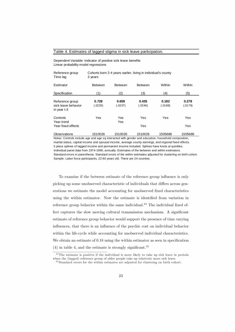
Table 4. Estimates of lagged stigma in sick leave participation.

Dependent Variable: Indicator of positive sick leave benefitsLinear probability model regressions

Reference group Cohorts born 2-4 years earlier, living in individual's countyTime lag 3 years

Estimator Between Between Between Within Within

Specification (1) (2) (3) (4) (5)

Reference group 0.728 0.659 0.435 0.182 0.278sick leave behavior (.0229) (.0237) (.0246) (.0188) (.0179)in year t-3

Controls Yes Yes Yes Yes YesYear trend YesYear fixed effects Yes Yes

Observations 1510026 1510026 1510026 1505686 1505686Notes: Controls include age and age sq interacted with gender and education, household composition, marital status, capital income and spousal income, average county earnings, and regional fixed effects. 5 piece splines of lagged income and permanent income included. Splines have knots at quintiles. Individual panel data from 1974-1990, annually. Estimates of the between and within estimators.Standard errors in parenthesis. Standard errors of the within estimates adjusted for clustering on birth cohort.Sample: Labor force participants, 22-60 years old. There are 24 counties.

To examine if the between estimate of the reference group influence is only

picking up some unobserved characteristic of individuals that differs across gen-

erations we estimate the model accounting for unobserved fixed characteristics

using the within estimator. Now the estimate is identified from variation in

reference group behavior within the same individual.44 The individual fixed ef-

fect captures the slow moving cultural transmission mechanism. A significant

estimate of reference group behavior would support the presence of time varying

influences, that there is an influence of the psychic cost on individual behavior

within the life-cycle while accounting for unobserved individual characteristics.

We obtain an estimate of 0.18 using the within estimator as seen in specification

(4) in table 4, and the estimate is strongly significant.45

44The estimate is positive if the individual is more likely to take up sick leave in periodswhen the (lagged) reference group of older people take up relatively more sick leave.45 Standard errors for the within estimates are adjusted for clustering on birth cohort.

23

Under the assumption that average reference group behavior is perfectly

correlated with fixed work norms attained as a child (fixed characteristics) the

estimate 0.73 in specification (1) provides an upper bound for the combined

effect of time varying and fixed influences of the reference group on individual

behavior. The within estimate of 0.18 does not include any effect of the fixed

characteristics but only the time varying influences.46 The ratio of the within

estimate to the between estimate could be interpreted as a lower bound on the

importance of time varying influences compared to cultural transmission.47 Our

estimates indicate that at least one quarter of the total influence of reference

group behavior is attributable to time varying influences.48 For the reasons

discussed we don’t think this number should be taken literally but it supports

the hypothesis that both mechanisms are quantitatively significant.

We find that there is a significant impact of reference group behavior on

sick leave take up in our estimation across individuals also after accounting for

flexible time effects. In specification (2) we include a linear time trend in the

between estimation, which controls for a linear increase in the demand for sick

leave over time. The coefficient estimate on reference group behavior drops

but it is still strongly significant. We also allow for non linearities in the time

effects by including time fixed effects in specification (3).49Again, the coefficient

estimate on the reference group behavior drops but it is still significant.

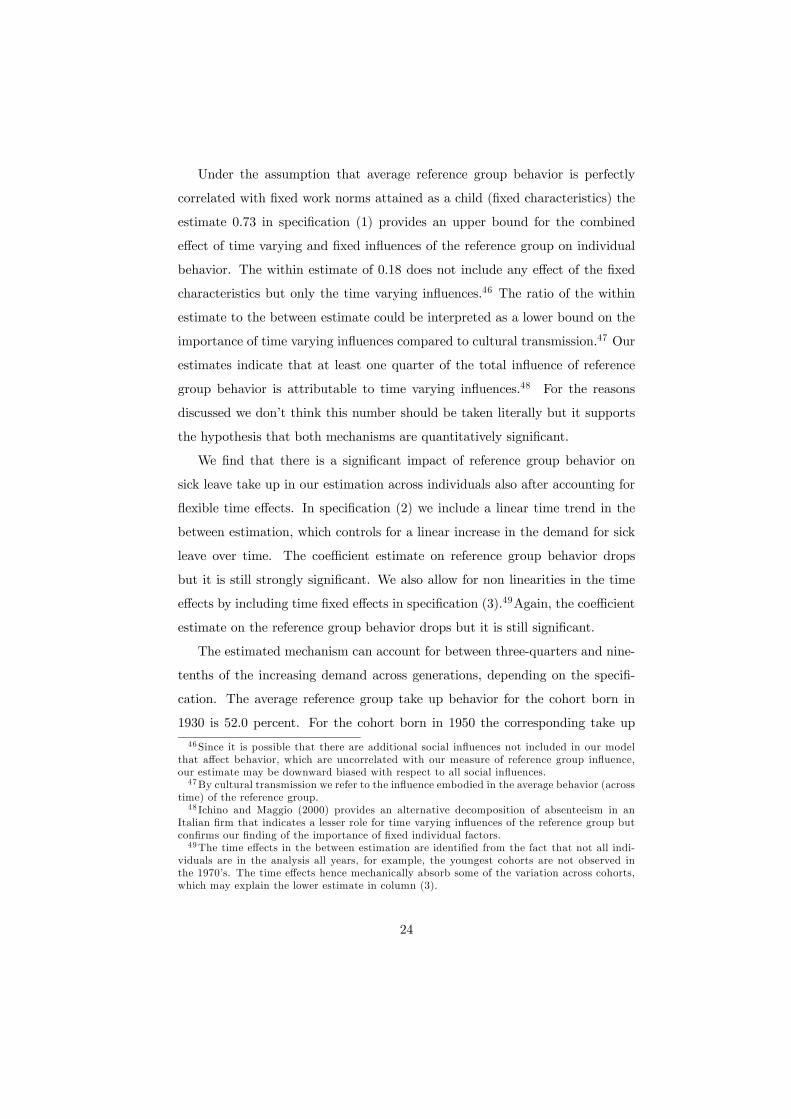
The estimated mechanism can account for between three-quarters and nine-

tenths of the increasing demand across generations, depending on the specifi-

cation. The average reference group take up behavior for the cohort born in

1930 is 52.0 percent. For the cohort born in 1950 the corresponding take up

46Since it is possible that there are additional social influences not included in our modelthat affect behavior, which are uncorrelated with our measure of reference group influence,our estimate may be downward biased with respect to all social influences.47By cultural transmission we refer to the influence embodied in the average behavior (across

time) of the reference group.48 Ichino and Maggio (2000) provides an alternative decomposition of absenteeism in an

Italian firm that indicates a lesser role for time varying influences of the reference group butconfirms our finding of the importance of fixed individual factors.49The time effects in the between estimation are identified from the fact that not all indi-

viduals are in the analysis all years, for example, the youngest cohorts are not observed inthe 1970’s. The time effects hence mechanically absorb some of the variation across cohorts,which may explain the lower estimate in column (3).

24

is 68.9 percent. Using the between estimate of 0.73 in column (1) we get that

the psychic cost increases the younger cohort’s take up rate by 12.3 percentage

points, which is close to what we estimated in table 2.50 If we use the estimate in

column (3) the effect is a 7.3 percentage points increase for the younger cohort

due to the psychic cost.51

Returning to the within estimator we may account for time effects also

here.52 Including the year fixed effects alters the interpretation on the estimated

coefficient on reference group behavior. Without year fixed effects the coefficient

is identified from mean deviations of reference group behavior. With year fixed

effects the within coefficient estimate is identified from mean deviations of ref-

erence group behavior and mean deviations from the national average take up,

basically a double difference. The estimated coefficient in specification (5) in-

dicates a stronger influence of reference group behavior conditional on national

behavior.53 , 54

6.3 Instrumenting for reference group behavior

To further examine our hypothesis we use an instrument to get exogenous shifts

in sick leave behavior of the reference group. We use reference group mortality

rates to instrument for reference group behavior.55 The idea is that mortality

rates are the result of serious health shocks, which also affect sick leave take

up. Implicitly, we only consider variation in reference group behavior that is

50The raw average in column (1) of table 2 indicates a 16 percentage point higher take uprate for the cohort born 20 years later. The estimate in column (6) of table 2 produces a 13.4percentage point higher take up rate for the younger cohort.51This number may be most comparable to specification (5) in table 3, which indicates a

difference in take up of 9.6 percentage points for cohorts born 20 years apart.52 Introducing a linear time trend is not meaningful in the within context since we are already

controlling for age, which contains the same variation as a time trend.53The estimate in specification (5) is not directly comparable to specification (3) since the

between estimate does not have a similar double difference interpretation.54The estimated within coefficients can’t be used to account for the differences in demand

across cohorts since all the differences across cohorts are absorbed by the individual fixedeffects.55The instrument is not intended to explain the cohort trend in sick leave, the mortality

rate just provides exogenous variation in the reference group’s behavior.

25

correlated with these serious health shocks.56

We observe mortality rates per 1000 population by year, age and county. We

assume that mortality follows a simple model with a second order polynomial

in age and a random shock. If we denote the mortality rate in county c, for the

generation born in year g, in year t by MRc,g,t we have

MRc,g,t = α0 + α1Aget + α2Age2t + εc,g,t (9)

We assume that the mortality shocks are i.i.d. across counties, generations, and

years. The model explains about 85 percent of the variation in the data. As our

main regression includes controls for age and its square it’s only the remaining

variation in the error term that is used to provide exogenous variation in ref-

erence group behavior. We could also allow more complex models of mortality,

for example with year fixed effects57 but it would not affect our analysis in the

specifications that control for year fixed effects.

The mortality rates we use as instruments are defined in the same way the

reference group behavior is defined. That is, the mortality rate per 1000 of those

born 2-4 years earlier by county, lagged 3 years, is used to instrument for the

sick leave take up by those born 2-4 years earlier by county, lagged 3 years. The

identifying assumption for this approach is that older cohorts’ mortality rates

have no direct impact on individual sick leave decisions three years later. The

only impact comes through the older cohorts’ behavior.58

We estimate our models by two stage least squares (2SLS). The instrument

exhibits variation across counties, generations, and years. The first stage re-

gressions show a positive relationship between mortality rates and sick leave up

take. The instrument is not weak.59

56These serious health shocks contrast with arguably less serious shocks to the value ofleisure such as big athletic events, see Skogman-Thoursie (2004).57Adding year fixed effects to the model increases the explanatory power by about 1 per-

centage point. In a model with year effects we could relax the assumption that health shocksare independent across counties and allow for common time trends.58More formally, the assumption is that the mortality shocks in (9) for the generations 2-4

years older in year t-3 are uncorrelated with the leisure shocks to the current generation inyear t in the main model (7).59The instrument has t-values of at least 5 in first stage regressions, and tests based on

Kleibergen-Paap statistics reject the hypotheses of weak instruments and underidentification.The results are robust to including county fixed effects rather than regional fixed effects.

26

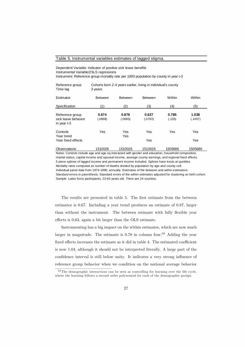
Table 5. Instrumental variables estimates of lagged stigma.

Dependent Variable: Indicator of positive sick leave benefitsInstrumental Variable/2SLS regressionsInstrument: Reference group mortality rate per 1000 population by county in year t-3

Reference group Cohorts born 2-4 years earlier, living in individual's countyTime lag 3 years

Estimator Between Between Between Within Within

Specification (1) (2) (3) (4) (5)

Reference group 0.674 0.876 0.627 0.785 1.038sick leave behavior (.0898) (.0695) (.0793) (.135) (.1457)in year t-3

Controls Yes Yes Yes Yes YesYear trend YesYear fixed effects Yes Yes

Observations 1510026 1510026 1510026 1505686 1505686Notes: Controls include age and age sq interacted with gender and education, household composition, marital status, capital income and spousal income, average county earnings, and regional fixed effects. 5 piece splines of lagged income and permanent income included. Splines have knots at quintiles. Mortality rates computed as number of deaths divided by population by age and county cell.Individual panel data from 1974-1990, annually. Estimates of the between and within estimators.Standard errors in parenthesis. Standard errors of the within estimates adjusted for clustering on birth cohort.Sample: Labor force participants, 22-60 years old. There are 24 counties.

The results are presented in table 5. The first estimate from the between

estimator is 0.67. Including a year trend produces an estimate of 0.87, larger

than without the instrument. The between estimate with fully flexible year

effects is 0.63, again a bit larger than the OLS estimate.

Instrumenting has a big impact on the within estimates, which are now much

larger in magnitude. The estimate is 0.78 in column four.60 Adding the year

fixed effects increases the estimate as it did in table 4. The estimated coefficient

is now 1.04, although it should not be interpreted literally. A large part of the

confidence interval is still below unity. It indicates a very strong influence of

reference group behavior when we condition on the national average behavior

60The demographic interactions can be seen as controlling for learning over the life cycle,where the learning follows a second order polynomial for each of the demographic groups.

27

through the year effect.

Overall, the estimated influence of role model behavior is larger when we

instrument using mortality rates. Role model behavior shifted by these health

shocks has a substantial influence on individual behavior. It is also possible

that instrumenting has removed bias due to mismeasurement of role model

influence, which would lead to higher estimates. The estimates in table 5 are

fairly similar across specifications. The range 0.75 to 0.78 are within the 95

percent confidence intervals of all the estimates. That the between and within

estimates aren’t substantially different would indicate the there aren’t omitted

variables correlated with sick leave behavior that drive the result as the omitted

factors controlled for in the individual fixed effect doesn’t affect the estimates

much.

The coefficients in table 5 can’t be used to assess the relative importance

of fixed versus time varying influences as we did in table 4. The purpose of

using the instrument is to isolate the influence of role model behavior through

the channel of exogenous health shocks. By doing so we avoid the potential

influence of culture (fixed influences) discussed above.

Challenges to our identification include omitted time trends at the county

level that correlate with both reference group mortality and behavior. One

candidate may be differential trends in productivity across counties, as individ-

uals in counties with low productivity growth may find it increasingly beneficial

to take sick leave relative to counties with high productivity growth. If these

productivity trends were correlated with mortality rates it may confound the

effect we set out to estimate. However, we control for average labor earnings by

county to capture such trends.61

Furthermore, our results are robust to including the current mortality rate of

the individual’s own cohort as a control variable, as seen in table 6.62 ,63 ,64Omitted

61Our results are also robust to controlling for county level fixed effects.62The results are also robust to controlling for the own cohort’s mortality rate lagged 3

years (rather than the current rate).63This may be interpreted as relaxing the assumption that the health shocks in (9) are

independent across generations and time.64The relatively weak influence of the own cohorts mortality rate in table 6 may seem at

28

trends that would challenge our identification would not only have to correlate

with the reference group’s mortality and sick leave across counties, cohorts,

and time; the trends would also have to be uncorrelated with the own cohort’s

mortality rate. Hence, these county level trends would have to differ in a very

particular way for generations born a few years apart.

Table 6. Instrumental variables estimates while controlling for own cohort's mortality rate.

Dependent Variable: Indicator of positive sick leave benefitsInstrumental variables (2SLS) regressionsInstrument: Reference group mortality rate per 1000 population by county in year t-3

Reference group Cohorts born 2-4 years earlier, living in individual's countyTime lag 3 years

Estimator Between Between Between Within Within

Specification (1) (2) (3) (4) (5)

Reference group 0.668 0.823 0.476 0.758 1.019sick leave behavior (.1227) (.0999) (.1183) (.1381) (.1521)in year t-3

Own cohort's mortality 0.0002 0.0028 0.0072 0.0014 0.0008rate in year t (.0028) (.0031) (.0032) (.0007) (.0007)

Controls Yes Yes Yes Yes YesYear trend YesYear fixed effects Yes Yes

Observations 1510026 1510026 1510026 1505686 1505686Notes: Controls include age and age sq interacted with gender and education, household composition, marital status, capital income and spousal income, average county earnings, and regional fixed effects. 5 piece splines of lagged income and permanent income included. Splines have knots at quintiles. Mortality rates computed as number of deaths divided by population by age and county cell.Individual panel data from 1974-1990, annually. Estimates of the between and within estimators.Standard errors in parenthesis. Standard errors of the within estimates adjusted for clustering on birth cohort.Sample: Labor force participants, 22-60 years old. There are 24 counties.

We argue that our approach deals with potential sorting, for example that

individuals with a high valuation of leisure could move to places where the psy-

odds with the first stage results. However, we may separate the mortality shocks into one partrelated to sick leave and one part that is unrelated to sick leave. The part that is unrelatedto sick leave only produces noise in the estimation, and our results indicate that this noise iscancelled out when averaged across cohorts.

29

chic cost of claiming sick leave benefits is low. First, the individual fixed effect

accounts for that individuals differ in their valuation of leisure in unobservable

ways wherever they reside. Second, in the within specifications we use unex-

plained mortality shocks to get exogenous variation in reference group behavior.

The mortality shocks are hence positive some years, and for some cohorts, and

negative in other periods. Migration flows don’t match the patterns of unex-

plained mortality shocks.

Our results don’t rely on the particular reference group or the time lag. We

find similar results when the time lag is 1 year or 5 years. The results are also

similar if we redefine the reference group to those 2-6 years older, or those 1-3

years older (and these changes are also robust to changing the time lag).65As

a falsification test we have also estimated a model where we use the 3 year

lead of the 2-4 years older cohorts’ behavior. The lead should not have an

impact on current behavior according to our hypothesis. The estimated effect

is insignificant at conventional levels, in line with our hypothesis.

We believe the analysis builds a strong case for causality; that reference

group behavior, as shifted by mortality shocks, has a direct influence on in-

dividual sick leave decisions. The identifying assumption is that there aren’t

omitted local trends that correlate with reference group mortality and behavior

but are uncorrelated with the mortality of those a couple of years younger. We

may entertain stories that there are local trends in for example drug abuse that

affect both sick leave and mortality. Such trends could potentially challenge

our identification since both reference group sick leave and mortality as well as

individual sick leave could be affected by the same drug abuse trend. It is reas-

suring that the influence of role model behavior is robust to including the own

cohort’s mortality rate, as the own group’s mortality would capture the drug

abuse trend.66Using reference group mortality as an instrumental variable, and

65We have also estimated a model where the reference group is 2-4 year younger, whichwould correspond to a model with young ’trend setters’. We find a significant effect, althoughit’s significance is much lower than for the model with older reference groups. For this reasonwe prefer the model with older reference groups.66 If the drug abuse trend did not affect mortality it would not be a challenge in the first

place since it would be uncorrelated with reference group mortality, and hence not part of the

30

controlling for the mortality of the individual’s own cohort, makes a compelling

case that we have identified one channel of intertemporal influence in sick leave

choices.

7 Conclusion

How do individuals adapt to institutions? Plenty of evidence show that in-

stitutions shape different outcomes across locations.67 However, precious little

evidence exists on how these outcomes come about. Basically, we know that

societies and communities end up with different outcomes based on the institu-

tions they face or faced, but we know very little about how they got there.

We study the adaptation in demand for social insurance over time and

across generations in Sweden following an expansion of the social insurance

programs. Our evidence shows how individuals adapt to the expanded welfare

state. We document substantial differences in behavior, almost one percentage

point higher program up take per birth cohort, although program rules have

been constant for decades.

We model a preference mechanism and evaluate to what extent it can ex-

plain the rapid increase in benefits take up across cohorts. We allow individuals’

benefit take up decision to depend on the behavior of ’role models.’68 We find

a significant influence of role model behavior on individual benefit take up,

which can account for a majority of observed behavioral differences across co-

horts. This is the first paper to estimate the dynamic adaptation of norms to

behavior in the welfare state, as little empirical evidence exists regarding what

forces shape norms. The underlying mechanism we study is present in several

literatures69 yet few papers empirically evaluate how economic outcomes affect

preferences and norms.

variation we use to identify our estimate.67 See for example Bisin and Verdier (2010), Fernandez (2010), and Tabellini (2008).68Preferences are modeled such that the threshold for claiming benefits depends on your

experience with role model behavior.69The program participation literature talks about stigma affecting choices. The literature

on culture asks how beliefs affect economic outcomes. Doepke and Zilibotti (2008) model theevolution of work norms.

31

We provide evidence on how norms evolve and how they affect behavior using

a large individual panel data set. We exploit variation across different gener-

ations as well as variation across time within individuals to estimate a model

where the take up decisions depend on the past behavior of role models. We find

that being exposed to older generations that used the sick leave program more

is associated with higher individual demand for the program. We use reference

group mortality rates to instrument for reference group behavior to address con-

cerns that omitted variables, such as local health or productivity trends, may

drive our results. We find that movements in reference group behavior due to

mortality shocks have a substantial impact on individual decisions to take up

sick leave. The IV/2SLS results point to a strong and robust intertemporal

influence of reference group behavior on individual decisions.

We focus on the take up of sick leave benefits in Sweden, since this decision is

purely determined by individual demand. Individuals assess themselves if they

are unfit to work and want to collect sick leave benefits. Changing behavior can

be seen as an estimate of how the self assessed threshold for claiming benefits

change. The specifics of the program lend it to study of the intertemporal

mechanism we model, but our mechanism and our results are quite general. Our

intertemporal mechanism does not preclude that for example spatial interactions

are present or that there are additional intertemporal mechanisms. We find

that our model captures a quantitatively significant mechanism, and with our

instrumented results we provide compelling evidence that the intertemporal

mechanism is indeed one channel of influence on individual decisions.

The intertemporal adaptation mechanism we estimate may apply to all kinds

of welfare state programs. Our findings, that younger generations use social in-

surance more than the older generations, correspond with survey evidence on

attitudes towards claiming public benefits among the young. Younger genera-

tions have a higher acceptance of claiming public benefits one is not entitled

to according to the World Values Survey.70 This is a consistent finding across

70The wording of the question is ’Do you think it can always be justified, never be justified,or something in between, to claim government benefits to which you are not entitled.’

32

countries, including Sweden, and indicates that the intertemporal mechanism

at work in Sweden could be relevant elsewhere.71 Our model could apply to

other social insurance programs and to programs with different levels of gen-

erosity as the intertemporal mechanism does not depend on program generosity

or particulars of the program.

Being exposed to welfare state institutions may have a profound effect on

individuals’ behavior. The increasing take up rates of benefits across cohorts

in figure 1 plainly show that a substantial shift in society is in progress. We

postulate and estimate a particular mechanism to explain the trend. Experience

with role models who demand more social insurance result in higher individual

demand, both when compared across generations and along the life cycle path

within generations. Our analysis indicates that large policy reforms don’t take

place in a static environment. Individuals gradually adapt to the environment

and demand more benefits. For generations born a few decades apart this

adds up to a fundamental shift in behavior where the young have much higher

demands on public programs. Quantifying the adaptation process to the public

policy, and estimating a specific mechanism using a new empirical strategy are

our unique contributions to the literature.

References[1] Abel, Andrew B., “Optimal Taxation When Consumers Have Endogenous

Benchmark Levels of Consumption,” Review of Economic Studies, LXXII(2005), 1—19.

[2] Aghion, Philippe, Yann Algan, and Pierre Cahuc (2008). "Can Policy In-teract with Culture? Minimum Wage and the Quality of Labor Relations."Working paper.

[3] Aghion, Philippe, Yann Algan, Pierre Cahuc, and Andrei Shleifer (2010)."Regulation and Distrust ." Quarterly Journal of Economics 125:3.

[4] Alesina, Alberto and Nicola Fuchs-Schündeln (2007). "Goodbye to Lenin(or not?): The effect of Communism on people’s preferences." AmericanEconomic Review, Volume: 97, Issue: 4, 1507-1528.

71This pattern is robust to controlling for gender, education, employment status, maritalstatus, income, country fixed effects, and survey wave effects.

33

[5] Algan, Yann, and Pierre Cahuc (2010). "Inherited Trust and Growth."Forthcoming, the American Economic Review.

[6] Beaman, Lori, Raghabendra Chattopadhyay, Esther Duflo, Rohini Pande,Petia Topalova (2009). "Powerful Women: Does Exposure Reduce Bias?"Quarterly Journal of Economics, 124:4, 1497-1540.

[7] Beaulieu, N., J.-Y. Duclos, B. Fortin, and M. Rouleau (2005). "Intergen-erational reliance on social assistance: Evidence from Canada." Journal ofPopulation Economics 18 (3), 539-562.

[8] Benhabib, Jess, Matthew O. Jackson, and Alberto Bisin, editors (2010)."Handbook of Social Economics." North Holland, forthcoming.

[9] Bertrand, Marianne, Erzo Luttmer, and Sendhil Mullainathan (2000)."Network Effects and Welfare Cultures." Quarterly Journal of Economics,August, pp. 1019-1055.

[10] Bertrand, Marianne, and Sendhil Mullainathan (2001). "Do People MeanWhat They Say? Implications for Subjective Survey Data." The AmericanEconomic Review, Vol. 91, No. 2, pp. 67-72.

[11] Bisin, Alberto, Giorgio Topa, and Thierry Verdier (2004). "Religious In-termarriage and Socialization in the United States." Journal of PoliticalEconomy, vol. 112, no. 3, .615-64

[12] Bisin, Alberto, and Thierry Verdier (2001). “The Economics of CulturalTransmission and the Dynamics of Preferences.” Journal of Economic The-ory 97, 298-319.

[13] Bisin, Alberto, and Thierry Verdier (2000). "Beyond the melting pot: cul-tural transmission, marriage, and the evolution of ethnic and religioustraits." The Quarterly Journal of Economics, August, 955-988.

[14] Bisin, Alberto, and Thierry Verdier (2004). "Work Ethic and Redistribu-tion: A Cultural Transmission Model of the Welfare State." Mimeo, NewYork University.

[15] Bisin, Alberto, and Thierry Verdier (2010). The Economics of CulturalTransmission and Socialization. To appear in Handbook of Social Eco-nomics, Jess Benhabib, Alberto Bisin, Matt Jackson, eds., Elsevier.

[16] Blanchflower, David G., and Andrew J. Oswald, “Well-Being over Time inBritain and the USA,” Journal of Public Economics, LXXXVIII (2004),1359—1386.

[17] Boskin, Michael, and Eytan Sheshinski, “Optimal Redistributive TaxationWhen Individual Welfare Depends on Relative Income,” Quarterly Journalof Economics, XCII (1978), 589—601.

34

[18] Bruegger, Beatrix, Rafael Lalive, and Josef Zweimueller (2010). "Does Cul-ture Affect Unemployment? Evidence from the Röstigraben." Mimeo.

[19] Clark, Andrew E. (2003). "Unemployment as a social norm: psychologicalevidence from panel data." Journal of Labor Economics, 2003, vol. 21, no.2,323-351.

[20] Clark, Andrew E., Nicolai Kristensen, Niels Westergård-Nielsen (2009)."Economic Satisfaction And Income Rank In Small Neighbourhoods." Jour-nal of the European Economic Association, 7(2—3):519—527.

[21] Clark, Andrew E., and Andrew J. Oswald, “Satisfaction and ComparisonIncome,” Journal of Public Economics, LXI (1996), 359—381.

[22] Daly, Mary C., and Daniel J. Wilson. "Happiness, Unhappiness, and Sui-cide: An Empirical Assessment." Journal of the European Economic Asso-ciation, 2009 7(2—3):539—549.

[23] Doepke, Matthias and Fabrizio Zilibotti (2008). "Occupational choice andthe spirit of capitalism." The Quarterly Journal of Economics, May, 747-93.

[24] Dupor, Bill, and Wen-Fang Liu, “Jealousy and Equilibrium Overconsump-tion,” American Economic Review, XCIII (2003), 423—428.

[25] Dynan, Karen E. and Enrichetta Ravina . “Increasing Income Inequality,External Habits, and Self-Reported Happiness.” The American EconomicReview, P & P, vol. 97 no. 2 (2007), 226-31.

[26] Edin, P-A, P Fredriksson, and O Åslund (2003). “Ethnic enclaves and theeconomic success of immigrants - evidence from a natural experiment."Quarterly Journal of Economics, Vol. 118, No. 1, pp. 329-357.

[27] Fernandez, Raquel (2008). "Culture as Learning: The Evolution of FemaleLabor Force Participation over a Century." Mimeo, New York University.

[28] Fernandez, Raquel, Alessandra Fogli, and Claudia Olivetti (2004). "Moth-ers and sons: Preference formation and female labor force dynamics." TheQuarterly Journal of Economics, November, 1249-99.

[29] Ferrer-i-Carbonell, Ada, “Income and Well-Being: An Empirical Analysisof the Comparison Income Effect,” Journal of Public Economics, LXXXIX(2005), 997—1019.

[30] Graham, Carol, 2009. "Happiness around the World." Oxford UniversityPress.

[31] Graham, Carol, and Andrew Felton (2006). “Inequality and Happiness:Insights from Latin America.” Journal of Economic Inequality, 4, 107—122.

35

[32] Guiso, Luigi, Paola Sapienza, and Luigi Zingales (2006). "Does cultureaffect economic outcomes?" Journal of Economic Perspectives, volume 20,no 2, 23-48.

[33] Guiso, Luigi, Paola Sapienza, and Luigi Zingales (2009). "Cultural Biases inEconomic Exchange?" Quarterly Journal of Economics. 124(4), 1095—1131.

[34] Harris, Judith Rich (1995). "Where is the child’s environment? A groupsocialization theory of development." Psychological Review, Vol 102, No.3, 458-489.

[35] Harris, Judith Rich (1998). "The nurture assumption: why children turnout the way they do." New York: Free Press.

[36] Hassler, John, José V. Rodríguez Mora, Kjetil Storesletten, Fabrizio Zili-botti (2003). "The Survival of the Welfare State." The American EconomicReview, Vol. 93, No. 1 (Mar., 2003), pp. 87-112.

[37] Henrekson, M. and M. Persson (2004). "The Effects on Sick Leave ofChanges in the Sickness Insurance System." Journal of Labor Economics22 (1), 87-113.

[38] Hesselius P, P Johansson & P Nilsson, "Sick of Your Colleagues’ Absence?",Journal of the European Economic Association, April 2009, Vol. 7, No. 2-3,Pages 583-594.

[39] Ichino, Andrea, and Giovanni Maggi (2000). "Work Environment and Indi-vidual Background: Explaining Regional Shirking Differentials in a LargeItalian Firm." Quarterly Journal of Economics, Vol. 115, No. 3, August,1057-1090.

[40] Ireland, Norman J., “Status-Seeking, Income Taxation and Efficiency,”Journal of Public Economics, LXX (1998), 99—113.

[41] Kingdon, Geeta, and John Knight (2007). “Community, Comparisons andSubjective Well-Being in a Divided Society.” Journal of Economic Behav-iour & Organization, 64, 69—90.

[42] Layard, Richard, “Human Satisfactions and Public Policy,” Economic Jour-nal, XC (1980), 737—750.

[43] Lemieux, Thomas and W. Bentley MacLeod (2000). "Supply side hystere-sis: the case of the Canadian unemployment insurance system." Journal ofPublic Economics, 78, pp. 139-170.

[44] Lindbeck, Assar and Sten Nyberg (2006). ”Raising Children to Work Hard:Altruism, Work Norms and Social Insurance.” Quarterly Journal of Eco-nomics, November, 1473-1503.

36

[45] Lindbeck, Assar, Sten Nyberg, and Jörgen Weibull (1999). "Social Normsand Economic Incentives in the Welfare State". Quarterly Journal of Eco-nomics, vol. 114, no. 1, 1-35.

[46] Lindbeck, Assar, Sten Nyberg, and Jörgen Weibull (2003). "Social Normsand Welfare State Dynamics". Journal of the European Economic Associ-ation, April—May 1(2—3):533—542.

[47] Lindbeck, Assar, Mårten Palme, and Mats Persson (2008). "Social Inter-actions and Sick Leave." Mimeo, Stockholm University.

[48] Ljungqvist, Lars, and Harald Uhlig, “Tax Policy and Aggregate DemandManagement under Catching Up with the Joneses,” American EconomicReview, XC (2000), 356—366.

[49] Luttmer, Erzo F. 2005. "Neighbors as Negatives: Relative Earnings andWell-Being." Quarterly Journal of Economics. 120:3, pp. 963-1002.

[50] Manski, Charles F. (1993). "Identification of endogenous social effects: Thereflection problem." Review of Economic Studies, 60(3): 531-42.

[51] Moffit, R. (1983): An Economic Model of the Welfare Stigma. AmericanEconomic Review 73(5): 1023-35.

[52] Mulligan, Casey B. (1997). "Parental priorities and economic inequality."The University of Chicago Press.

[53] Ng, Yew-Kwang, “Relative-Income Effects and the Appropriate Level ofPublic Expenditure,” Oxford Economic Papers, XXXIX (1987), 293—300.

[54] Oreopoulos, Philip, Marianne Page, and Ann Huff Stevens, 2008. "TheIntergenerational Effects of Worker Displacement." Journal of Labor Eco-nomics, vol. 26, no. 3, pp. 455-483.

[55] Oswald, Andrew J., “Altruism, Jealousy and the Theory of Optimal Non-Linear Taxation,” Journal of Public Economics, XX (1983), 77—87.

[56] Ravallion, Martin, and Michael Lokshin, “Identifying Welfare Effects fromSubjective Questions,” Economica, LXVIII (2001), 335—357.

[57] Seidman, Laurence S., “Relativity and Efficient Taxation,” Southern Eco-nomic Journal, LIV (1987), 463—474.

[58] Skogman Thoursie, Peter, 2004. "Reporting Sick: Are Sporting EventsContagious?" Journal of Applied Econometrics, vol. 19, no. 6, 809-823.

[59] Solon, Gary (2002). "Cross-Country Differences in Intergenerational Earn-ings Mobility." The Journal of Economic Perspectives, Vol. 16, No. 3, pp.59-66.

37

[60] Solon, Gary, Mary Corcoran, Roger Gordon, and Deborah Laren. "Siblingand Intergenerational Correlations in Welfare Program Participation." TheJournal of Human Resources, Vol. 23, No. 3 (Summer, 1988), pp. 388-396.

[61] Stutzer, Alois and Rafael Lalive (2004). "The role of social work normsin job searching and subjective well-being." Journal of the European Eco-nomic Association, 2 (4), 696-719.

[62] Tabellini, Guido (2008). "The scope of cooperation: values and incentives."The Quarterly Journal of Economics, August, pages 905-950.

[63] Van de Stadt, Huib, Arie Kapteyn, and Sara van de Geer, “The Relativityof Utility: Evidence from Panel Data,” Review of Economics and Statistics,LXVII (1985), 179—187.

38