ad-a273 809 - defense technical information center · • ad-a273 809 •:s4 ,". -. ......

• AD-A273 809

S4 ,". -.•:

• ~ARMY RESEARcH LAORATORY

Monte Carlo Analysis of GPS PerformanceBased on Artillery Flight Mission and

Antenna Interaction

by George Wiles

ARL-TR-289 November 1993

DTICA ELECTE

DEC 16 1993 IS~E

.K 93-30386J • I II~~~~ ~~~Hlllilllll llnlrcr,

Approved for public release; distribution unlimited.

98 12 15022

The findings in this report are not to be construed as an official Department ofthe Army position unless so designated by other authorized documents.

Citation of manufacturer's or trade names does not constitute an officialendorsement or approval of the use thereof.

Destroy this report when it is no longer needed. Do not return it to theoriginator.

REPORT DOCUMENTATION PAGE ~o. opo8o8e ,P•*ie mpmB~g bdmn I•r Sib oOacml of ki dn a buma" U W i e 1 h per im m.. = b en.for werAwo u m I m bgawkmg u¢ S mu neadad. ad mepsii i uanf• i Vi meSeino bdlam daai said Cafuwi remq i ••bads ea or al 0M PP of 0ca~edaMI ~W dun~ml. ki damforiedualq 0* Vandal. ou Waafbnoli r Sa saes. IneeMr Opermam aid APOM. 1215 J0Mww0av" S, w 120 ,vA Hi.43• ,,id 20 Ad noe.f aidown, P.pe'aid, Rejn a.d 10o4-oIUA) Io OC O*503

I. AGENCY USE ONLY taw bb* 2. REPORT DA E REPrrT TYPE AM DATES COVERED

- November 1993 Final, 1/92 to 2/93

4. TITLE AND SUBTITLE L FUNDING NtUBERS

Monte Carlo Analysis of GPS Performance Based on Artillery Flight DA PR: AH1 6Mission and Antenna Interaction PE: P62120

L. AUTHOR(S)

George Wiles

7. PERFORMING ORGANIZATION NAME(S) AND ADORESS(ES) . PEPPORMING ORGANIATION

U.S. Army Research Laboratory REPORT NUMBER

Attn: AMSRL-SS-FG ARL-TR-2892800 Powder Mill RoadAdelphi, MD 20783-1197

9. SPoNSORMGJUONIORMNG AGENCY NAMES) AND ADORESS(ES) 10. SPONSORUGMONrTORNG

U.S. Army Research Laboratory ,ENCY REPORT NUMBE

2800 Powder Mill RoadAdelphi, MD 20783-1197

11. SUPPLEMENTARY NOTES

AMS code: 612120.HI 60011ARL PR: 36E162

12&. D1STMRTNAVAILABo.uTY STATEMENT I. ISTRIBUTION CODE

Approved for public release; distribution unlimited.

13. ABSTRACT "xnamn w 200 ,

The accuracy of GPS (Global Positioning System) receivers depends on the geometry of the GPS

satellites used in the position calculation; the receiver has optimum performance when given anunobstructed view of the sky. Previous work has shown that L-band antennas mounted on 155-mmartillery projectiles have nulls or blind spots in their patterns.

A Monte Carlo analysis was performed to assess the impact on system accuracy that various sizednulls would have. The analysis found that a system using the full 24-satellite constellation is verytolerant of even large antenna nulls.

14. SUBJECT TERMS 1s. NUMBER OF PAGES

GPS, Global Positioning System, Monte Carlo, artillery 3216. PRICE CODE

17. SECURITY CLASSIFICATION 1. SECURITY CLASSIFICATION 19. SECURITY CLASSIFICATION 20. LIMITATION OF ABSTRACTOF REPOR OF THIS PAGE OF ABSTRACT

Unclassified Unclassified Unclassified ULNSN 7540-01-2M0,5500 Stondard Form 296 (Rev. 2-09)

Prei•ebd by ANSI Sld. Z39-182WI-02

ContentsPage

1. Introduction ........................................................................................................................... 5

2. GD O P Calculation .......................................................................................................... 63. Random ization of Param eters ........................................................................................ 7

3.1 Time of Day ........................................................................................................... 83.2 User Location .......................................................................................................... 83.3 Flight M ission Database ............................................................................................. 8

3.3.1 Illustrative Exam ple .................................................................................. 93.3.2 Trajectory M odel D atabase ...................................................................... 10

4. N orm alized Flight Tim e ............................................................................................... 125. Baseline Results .............................................................................................................. 136. M onte Carlo Repeatability ........................................................................................... 147. Baseline Case w ith Fixed Antenna Null ................................................................... 148. M onte Carlo Results ....................................................................................................... 15

9. Conclusions .......................................................................................................................... 16D istribution ............................................................................................................................... 31

Appendices

A. Firing Conditions for Artillery Missions Used in Monte Carlo Analysis .......... 17

B. Monte Carlo Results: Best Calculated GDOP versus Normalized FlightTim e and Antenna N ull Conditions ........................................................................... 21

Figures1. Antenna nulls ...................................................................................................................... 52. Geom etry for GDOP calculation ................................................................................ 63. A sim ple GDOP calculation .......................................................................................... 64. M onte Carlo GDOP calculation ................................................................................... 75. All possible m arbles ....................................................................................................... 96. Uniform m arble distribution ........................................................................................ 97. W eighted m arble distribution ................................................................................... 108. Short-, m edium -, and long-range flights ................................................................. 139. Three flights w ith norm alized flight tim e ................................................................. 13

10. Fixed antenna nulls used in baseline calculations ................................................. 1411. N ull (200) at tw o orientations for baseline calculation ............................................ 15

3

TablesPage

1. AFAS usage distribution ................................................................................................ 112. Summary of possible conditions based on firing tables .......................................... 123. Uniform flight distribution .......................................................................................... 124. Weighted flight distribution ........................................................................................ 125. Baseline GDOP calculation ........................................................................................... 146. Baseline case of various size antenna nulls ............................................................... 147. Baseline case of 200 null at different orientations ...................................................... 15

Accesion For

NTIS CRA&

DTIC TABU, LI-rounced El

B y - .. ..-- .... ----------

LD, t ib tio -Ip~vhbittyCo'les

. A v a, o r

4

1. Introduction

As part of an ongoing effort to improve artillery accuracy and effec-tiveness, the Global Positioning System (GPS) is being considered asa potential source of position information for artillery systems. Sev-eral concepts for projectile-mounted systems have been proposed.One concept involves tracking projectiles with a GPS transponder.Others involve placing a GPS receiver on a projectile for positionfuzing or guidance applications.

Several factors contribute to the position accuracy of a GPS trans-ponder or receiver system. One of these factors is the potential lackof isotropic coverage provided by the receive antenna. For optimumreceiver performance, an unobstructed view of the sky is required.However, previous experience with projectile-mounted antennasnear the GPS frequency has shown that there may be voids in thecoverage due to nulling produced by the interaction of the antennawith the projectile body (see fig. 1). It is necessary to quantify the ex-pected error due to the antenna nulls; to accomplish this, we per-formed a Monte Carlo analysis.

The accuracy of a GPS receiver may be considered to depend on twoindependent contributing factors. The first, the user range error(URE), accounts for the receiver's ability to measure the satellitesignal's phase, the uncertainty due to the tropospheric delay, algo-rithmic and computational error, satellite ephemeris, and other er-rors. The URE is independent of the geometry of the encounter. Thesecond factor, the geometric dilution of precision (GDOP), dependssolely on the relation of the positions of the satellites and the re-ceiver. The total error is the product of the URE and GDOP.

Figure 1. Antennanulls.

Rear nullangle

Receive antenna gain

5

2. GDOP CalculationThe GDOP is a geometric measure of the independence of the posi-tion information supplied by each satellite. In essence, it is a mea-sure of how well spaced the satellites used in the calculation are. Inthe four-satellite solution, solving for position and time error, wecalculate the GDOP from the root sum of the areas of the trianglesformed by the satellites, divided by three times the volume of thetetrahedron formed by the satellites and the user (see fig. 2). If thefour satellites and the user are in the same plane, then the tetrahe-dron volume is zero, and the GDOP is infinite. Generally, a GDOP of6 or less is considered usable; the fully deployed constellation of sat-ellites is designed to provide a GDOP of 6 or less for all users 90 per-cent of the time.

The calculation of the GDOP for any one circumstance is a trivialmatter. One must only determine the position of the satellites rela-tive to the receiver, find which of these satellites are not visible be-cause of antenna masking, and use the best calculated GDOP of thevisible satellites (see fig. 3).

Figure 2. Geometryfor GDOP calculation.

Figure 3. A simple Inputs CalculationsGDOP calculation.

Satellite almanac * Calculate satellite

Time of day O S0

S Choose 4 satellites

User location - Calculate relative:geometry

Caclt GDO

The answer

6

The difficulty in the analysis lies in incorporating the entire range ofpossible encounters given by the combination of artillery variables,antenna pattern, and satellite geometry. The Monte Carlo analysis isa useful way of exhaustively combining random inputs from rangesof variables and applying them to the process being studied. The re-sult of the analysis is a distribution of outcomes (GDOP's), whichhas statistical significance if enough combinations are examined. It isthis distribution that we need to assess the impact of antenna nullsin a system accuracy study.

3. Randomization of ParametersThree parameters of the GDOP calculation were to be independentlyrandomized: the time of day, the user location, and the artillery pro-jectile flight parameters (see fig. 4).

Figure 4. Monte Carlo Inputs CalculationsGDOP calculation.

Satellite almanac , Calculate satellite

Random time of day..'-

User location Calculate relative

/2' Random latitudeRandom longitude : Calculate GDOPs for

satellites above horizon

For each timeincrement:

Randomly selected light

Random firing azimuth Determine satelliteRi' visibility vs null angle

Front and rear antenna null

Select best GDOP fromvisible satellites

End of flight? Performanother random trial

7

3.1 Tune of Day

The proposed GPS satellite constellation consists of 24 satellites infixed 12-hour orbits. Thc --,;ition of each satellite can be preciselydetermined from the orbitii: q:-fiom,, -, Iich are a function of time.By uniformly randomizing time from 0 to !2 hcurtr, -,.. -n addressall the possible satellite positions. For the purpose of this exc.:"--circular approximation of the orbit sufficed.

3.2 User Location

To insure that the satellite positions were unbiased, I selected the lo-cation of the user on the earth's surface at random for each encoun-ter. Here it was assumed that any location on the surface is equallylikely (land or water); the longitude was allowed to vary uniformlybetween -180° and +1800, and the latitude varied as a cosine dis-tribution between -90° and +90°. The cosine latitude distributionaccounted for the fact that there is more surface area per degree oflatitude at the equator than at the poles. A spherical globe was used.The location variation is for geometric purposes only, and did notaffect the distribution of environmental factors, such as meantemperature, which in turn would affect the individual flightparameters.

3.3 Flight Mission Database

By far the most difficult parameter to assess was the distribution ofthe flight parameters. Some difficulties are the wide variations inflight duration that arise over all operating conditions, and the prob-lem of comparing a large quantity of disparate data. Because of thestatistical nature of a Monte Carlo analysis, it is not enough to knowthat a projectile could be launched either nearly horizontally ornearly vertically; one must also know how much more likely it is fora projectile to be launched at a certain angle. Since a mathematicaldescription of the distribution does not exist, a weighted set of rep-resentative trajectories was used.

For this study, I decided to create a database that not only representsevery possible trajectory, but also includes an indication of the rela-tive frequency with which that trajectory would be used in battleconditions. I provide an example to illustrate the rather convolutedmethod used to construct the distribution.

8

3.3.1 Illustrative Example

The International Marble Association is conducting scientific re-search into the effects of solar pressure on the travel of variousmarble types, to test the hypothesis that light colored marbles travelfarther with the sun at their back than do dark marbles. In a con-trolled experiment, randomly selected marbles were rolled across aprepared surface at different times of day. The experimenters wishto fill a jar with marbles so that at the conclusion of the experiment,when the marbles are sorted by class, the distribution of marblesmeets the prescribed IMA guidelines of 25-percent white, 25-percentblack, and 50-percent grey for all marbles in tournament play.

For the experiment .o be accurate, all varieties of marbles have to beconsidered (see fig. 5).

A preselection analysis determines that although light pink is amarble color, it is currently not allowed in tournament play. Afterlight pink is removed, the uniform distribution of classes is now asshown in figure 6.

The problem is now how to fill a jar with marbles so that the overallmix matches the IMA guidelines without distorting the representa-tion of the marbles within their class. By working toward a commonfactor of 4 x 3 = 12, we can create a modified distribution with threesets of white marbles, four sets of black marbles, and eight sets ofgrey marbles. This grouping satisfies the prescribed IMA guidelinesand represents all marbles within their class equally (see fig. 7).

Figure 5. All possiblemarbles. White Black Grey

zinc white 0 gloss black S granite 0off white 0 matte black 0 blue grey*

pearly white 0 off black 0 green grey Slight pink (

oyster 0

Figure 6. Uniform White Black Greymarble distribution.

Class 0 0 0 0 @0 0 0 0 GPercentage of total 40% 30% 30%

9

Figure 7. Weighted

marble distribution. 0 0 00 000 0 * a

0000 000 @000000 000 . 0

12/48=25% @00 0 0 @12/48=25% G 0 0

00624/48= 50%

A closer examination of the marble classes indicates that there aredistinct subclass groupings to consider, such as the three degrees ofoff-white marbles: antique white, bone white, and eggshell. This andother subclass groupings increase the size of the uniform distribu-tion of marbles (the number of distinct samples), and as the commonfactor grows, so does the minimum size of the weighted distribu-tion. The general technique to generate the weighted distributionwould be the same.

3.3.2 Trajectory Model Database

A similar method was used to create the flight mission database.Three classes of projectile firings were considered: short (0-15 km),medium (16-24 km), and long (25-50 km) range. Within each classare the various combinations of projectile type, charge, and firingangle (quadrant elevation, or QE) to strike a target within the rangeclass.

To create this flight mission database, I solicited help from the Artil-lery Effectiveness Working Group and the Field Artillery School atFort Sill. To make the undertaking manageable, we focused our ef-fort on the usage pattern of the Advanced Field Artillery System(AFAS). A preliminary study had been previously undertaken toidentify the mix of projectiles that would complement the AFASwhen fielded. With each projectile was an estimate of how often thatprojectile would be fired at short, medium, or long range. Table 1 isbased on that study.

This information was interpreted to mean that each AFAS systemwould enter the battle with 60 mixed rounds, and would shoot themat the ranges in the chart.

A modified three-degree-of-freedom (3DOF) ballistic computermodel was used to generate the position information for all theflights. Two parameters were used to differentiate the flights: charge

10

Table 1. AFAS usage Distribution of roundsdistribution. Rounds Type fired according to range

available 0-15 km 16-24 km 25-50 km

25 M483A1 52% (13) 48% (12)21 M795 62% (13) 24% (5) 14% (3)

5 M864 - - 100% (5)2 M549A1 - - 100% (2)7 M898 71% (5) 29% (2)

60 All 52% (31) 32% (19) 17% (10)

and range. Even though the AFAS may use liquid propellant, andtherefore be capable of a continuously variable muzzle velocity, theold system of 11 quantized charges (designated 3G, 3W, 4G, 4W, 5G,5W, 6W, 7W, 8, 8S, and UNI) was used. The ranges were quantizedin 1- and 2-km increments from 0 to 50 km, and the firing tableswere used to determine which quadrant elevations resulted in thoseranges for those charges. Often there are two valid QE solutions toreach a range at a certain charge. When both high-angle and low-angle solutions existed, only the low angle was used; this choice re-flects the general policy of limiting the flight time of the projectile tominimize its vulnerability. The remaining variables in the 3DOFmodel (temperature, tube wear, met conditions, etc) were set tonominal for all flights.

The resulting conditions for the AFAS database are in appendix A. Asummary of the conditions is shown in table 2, which shows, forexample, that there are 26 different ways for an M483A1 to hit ashort-range target. This table is further modified by the doctrineconstraints (for example, the M864 is only fired long range). Themodified distribution is referred to here as the uniform flight distri-bution (table 3), since there is no information as to how likely eachflight is to be used.

The combination of projectile and range category (short, medium,and long) is considered a class of flights. In order to create a set offlights that represent the AFAS usage distribution from the uniformdistribution of flights, we determined a weighting factor and ap-plied it to each class of flights, so that in the weighted set of flights,the percentage of all flights in a class will agree with the AFAS dis-tribution. The weighting factors were determined by trial and errorto approximate the AFAS distribution; see table 4.

For example, the 26 flights that make up the class of short-range fir-ings of the M483A1 would be represented eight times each in theweighted database. That class will then make up 208/936, or 22.2percent of the total usage. This corresponds to 13/60, or 21.7 percentof the original AFAS distribution.

11

Table 2. Summary of Firings according to rangepossible conditions Projectile Short Medium Longbased on firing tables. M483A1 26 15 1

M795 27 16 1M864 11 18 8M549A1 9 20 9M898 26 15 1

Table 3. Uniform Firings according to rangeflight distribution. Projectile Short Medium Long

M483A1 26 15M795 27 16M864 - - 8M549A1 - - 9M898 26 15

Table 4. Weighted AFAS Firing tables Weight factor I no. in class

flight distribution, distribution distribution

Projectile S M L S M L S M L

M483A1 13 12 - 26 15 - 81208 121180 -M795 13 5 3 27 16 - 81216 5180 45145M8`4 - - 5 - - 8 - - 9172M.,.-9A. - - 2 - - 9 - - 3127M898 5 2 - 26 15 - 3178 2130 -

Total = 60 Total = 142 Total flights = 936

4. Normalized Flight Time

So that the results, based on flights of differing lengths, can be com-pared, the flight times are normalized and presented as a percentageof the total flight. Twenty increments are used. For example, if aflight is 58 s long, then the parameters of interest (its position andvelocity) are calculated every 2.9 s. This information is then used tocalculate the best GDOP at each time increment, and the resultingGDOP's are stored in the 20 corresponding bins. At the end of theMonte Carlo analysis, there will be a distribution of GDOP's for each5 percent of the "typical" flight. This allows separate portions offlight to be considered. Figures 8 and 9 illustrate how the use of nor-malized flight time allows comparison of flights. The velocity vectoras well as the position of the projectile was required so that onecould determine the attitude of the projectile and hence the attitudeof its axial antenna nulls.

12

Figure 8. Short-, 8000medium-, and long-I- Irange flights. 6000-

- - • - - -

4000 / - --

.-• / ~,-,"" ".. -'

200 .. 0 j !

00 10 20 30 40 50 60 70 80

time (s)

Figure 9. Three flights 8000with normalized-flight time. 6 I I -' lII i" IN.60001 , , , , • ,

I I/ I I "I I I

I " I l ___ I4000time incremen

daaas-reea ined it .is informative to pefr aereso

< 2000 , ,. "1 , , / , ,. . ,-

l c i the "peman Idaabseareai ned, it is inomtv to pefr a sei e ofbaeln caclain to deemn thpromneforstel~lite

model when unperturbed by antenna nulls.

The first baseline calculation consisted of determining the lowestGDOP of all satellite combinations for 10,000 trials for random loca-tions on the globe, with the fixed variable being a horizon maskangle. Table 5 shows these results. The horizon mask angle is the el-evation above the horizon below which a satellite is consideredmasked by the terrain. For example, in table 5, the value of 2.509 for50-percent time and 0* mask angle indicates that 50 percent of thetime, or for half the Monte Carlo trials, the GDOP was 2.509 or better(smaller). The result agrees closely with the advertised figure ofmerit of a GDOP of 6.0 for 90 percent of the time with the full con-stellation intact and a 50 mask angle.

13

Table 5. Baseline Percentage GDOP according to horizon mask angleGDOP calculation. of time 00 50 100 150 200

50 2.509 2.821 3.323 3.856 4.65680 3.472 3.997 4.653 5.618 6.97690 5.047 5.934 6.939 8.092 10.876

6. Monte Carlo RepeatabilityMy colleague Leng Sim and I conducted the baseline experimentthree times under the same conditions to determine the variability ofthe results. Since the values are arrived at through many combina-tions of randomly selected parameters, one would not expect thesame result for each set of trials, unless an extremely large numberof trials was conducted. For our sample size of 10,000 trials, wefound that the results at the 50th, 80th, 90th, and 95th percentilesvaried from experiment to experiment by less than 5 percent.

7. Baseline Case with Fixed Antenna NullAn extension of the baseline case is the case of a fixed antenna nullpointing at the sky (see fig. 10). A surprisingly large null can be tol-erated. This is because the best geometry giving the lowest GDOPoccurs when the satellites are separated in the sky, and not close to-gether within a null. Given that there is a 5-percent variability in theanswers, then there is little difference at all for small antenna nulls(see table 6).

Figure 10. Fixed- -

antenna nulls used in ------

baseline calculations. ,"40

Table 6. Baseline case Percentage GDOP at various null sizes (half angle)oftvarious of time 0° 100 200 300 400 500 60°antenna nulls.

50 2.831 2.836 2.838 2.854 2.910 2.980 3.50880 3.992 3.923 3.986 4.022 4.141 4.778 N/A90 5.919 5.633 5.896 5.963 6.362 14.691 N/A

N/A indicates less than four satellites visible.

14

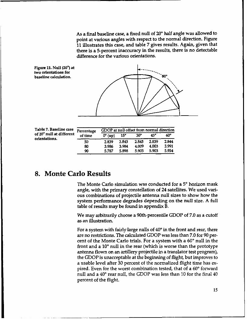
As a final baseline case, a fixed null of 200 half angle was allowed topoint at various angles with respect to the normal direction. Figure11 illustrates this case, and table 7 gives results. Again, given thatthere is a 5-percent inaccuracy in the results, there is no detectabledifference for the various orientations.

Figure 11. Null (200) attwo orientations forbaseline calculation.

Table 7. Baseline case Percentage GDOP at null offset from normal directionof 200 null at different of time 0* (up) 150 300 458 600orientations.

50 2.839 2.843 2.845 2.839 2.84480 3.986 3.984 4.009 4.003 3.99190 5.787 5.898 5.903 5.903 5.954

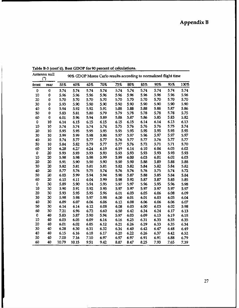
8. Monte Carlo ResultsThe Monte Carlo simulation was conducted for a 5* horizon maskangle, with the primary constellation of 24 satellites. We used vari-ous combinations of projectile antenna null sizes to show how thesystem performance degrades depending on the null size. A fulltable of results may be found in appendix B.

We may arbitrarily choose a 90th-percentile GDOP of 7.0 as a cutoffas an illustration.

For a system with fairly large nulls of 400 in the front and rear, thereare no restrictions. The calculated GDOP was less than 7.0 for 90 per-cent of the Monte Carlo trials. For a system with a 600 null in thefront and a 100 null in the rear (which is worse than the prototypeantenna flown on an artillery projectile in a translator test program),the GDOP is unacceptable at the beginning of flight, but improves toa usable level after 30 percent of the normalized flight time has ex-pired. Even for the worst combination tested, that of a 60* forwardnull and a 400 rear null, the GDOP was less than 10 for the final 40percent of the flight.

15

9. ConclusionsThe baseline calculations show that the Global Positioning System,because of the satellite geometry, is very tolerant of a null in the re-ceiver antenna pattern. It is somewhat less tolerant of horizon mask-ing, which would not be a problem in an airborne application. Theseobservations make sense when one considers the tetrahedral volumethat the geometric dilution of precision is based upon.

Overall, the artillery system was found to perform surprisingly wellwith substantial antenna nulls. As expected, the performance wasbetter at the end of flight for cases with large forward nulls, whenthe null would be pointed at the ground.

16

Appendix A. Firing . "ns for Artillery MissionsUsed in Monte Carlo Ana!vsis

Tables

Page

A-1. Projectile M483A1 ..................................................................................................... 18A-2. Projectile M795 ........................................................................................................... 18A -3. Projectile M 549 .......................................................................................... I ..................... 19A-4. Projectile M864 ........................................................................................................... 19A-5. Projectile M898 ........................................................................................................... 20

17

Appendix A

Tables A-1 to A-5 g±_: . quadrant elevations and charge conditionsused in the three-degree-of-freedom computer model to 'Zeneratethe trajectory database. These values were extracted from publishedand preliminary firing tables.

Table A-1. Projectile Range Quadrant elevation (Mils) according to chargeM483A1. (m) 4W 5G 5W 6W 7W 8 8R UNI

8000 602 524 465 356 2709000 680 566 416 310

10000 775 488 356 25811000 585 412 29512000 790 478 33613000 560 38314000 680 438 29215000 501 325

16000 578 365 27017000 690 415 29618000 470 33319000 530 370 .J20000 600 41221000 705

22000 51024000 635

25000 7302600028000 =30000

Table A-2. ProjectileM795. Range Quadrant elevation (mils) according to charge

(m) 4W 5G 5W 6W 7W 8 8R UNI

8000 562 500 435 322 2269000 660 538 387 274

10000 745 463 327 21511000 559 386 25512000 732 453 30013000 535 349 21014000 650 404 24315000 467. 279

16000 541 319 23217000 636 363 26418000 411 29819000 466 33620000 528 37621000 60222000 704 46824000 580

26000 7482800030000

18

Appendix A

Table A-3. Projectile Range Quadrant elevation (mils) according to chargeM549. (m) 4W 5G 5W 6W 7W 8 8R UNI

80009000

10000 22111000 25412000 29013000 331 22714000 376 25715000 426 291

16000 481 32817000 544 369 23518000 618 413 26219000 716 461 29120000 515 322 24022000 648 392 29023000 74624000 471 346

26000 564 40828000 681 47430000 887 54532000 62034000 69835000 741360003800040000


80009000 239

10000 27711000 31912000 364 23413000 414 26414000 471 29715000 538 333

16000 618 374 23917000 758 418 26518000 468 29219000 524 32120000 589 354 25521000 67122000 425 30024000 510 360

26000 620 41528000 838 47830000 55232000 64034000 74035000 8153600038000 1940000

Appendix A


8000 602 524 465 356 2709000 680 566 416 310

10000 775 488 356 25811000 585 412 29512000 790 478 33613000 560 38314000 680 438 29215000 501 325

16000 578 365 27017000 690 415 296

18000 470 333

19000 530 370

20000 600 412

21000 70522000 510

24000 635

25000 730260002800030000

20

Appendix B. Monte Carlo Results: Best CalculatedGDOP versus Normalized Flight Time and

Antenna Null ConditionsTables

Page

B-1. Best GDOP for 50 percent of calculations .............................................................. 22B-2. Best GDOP for 80 percent of calculations ............................................................. 24B-3. Best GDOP for 90 percent of calculations ............................................................. 26B-4. Best GDOP for 95 percent of calculations ............................................................. 28

21

Appendix B

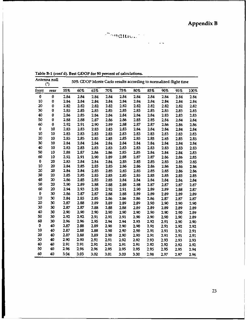
The values in table B-1 correspond to the best calculated GDOP atthe given percentage of flight increment for the specified antennanull angles. For the Monte Carlo analysis of 10,000 trials, 50 percentof the trials resulted in a calculated GDOP that was better (smaller)than that in the table.

Table B-1. Best GDOP for 50 percent of calculations.

Antenna null 50% GDOP Monte Carlo results according to normalized flight time(°)

front rear 5% 10% 15% 20% 25% 30% 35% 40% 45% 50%

0 0 2.84 2.84 2.84 2.84 2.84 2.84 2.84 2.84 2.84 2.8410 0 2.85 2.84 2.84 2.84 2.84 2.84 2.84 2.84 2.84 2.8420 0 2.84 2.84 2.84 2.84 2.84 2.83 2.83 2.83 2.83 2.8230 0 2.89 2.89 2.88 2.88 2.88 2.87 2.87 2.87 2.86 2.8640 0 2.91 2.91 2.90 2.90 2.89 2.89 2.88 2.88 2.87 2.8650 0 2.97 2.96 2.95 2.95 2.94 2.93 2.92 2.91 2.90 2.8960 0 3.04 3.02 3.01 3.00 2.98 2.98 2.96 2.95 2.94 2.930 10 2.83 2.83 2.83 2.83 2.83 2.83 2.83 2.83 2.83 2.8310 10 2.83 2.83 2.83 2.83 2.83 2.83 2.83 2.83 2.83 2.8320 10 2.87 2.86 2.86 2.86 2.86 2.85 2.85 2.85 2.85 2.8530 10 2.88 2.88 2.87 2.87 2.87 2.86 2.86 2.85 2.85 2.8540 10 2.82 2.82 2.82 2.82 2.82 2.82 2.82 2.82 2.82 2.8350 10 2.95 2.95 2.94 2.94 2.93 2.92 2.91 2.90 2.89 2.8960 10 3.03 3.01 3.00 2.99 2.98 2.96 2.95 2.94 2.93 2.930 20 2.82 2.82 2.82 2.82 2.82 2.82 2.82 2.83 2.83 2.83

10 20 2.84 2.84 2.84 2.84 2.84 2.84 2.84 2.84 2.84 2.8420 20 2.85 2.85 2.85 2.85 2.84 2.84 2.84 2.84 2.84 2.8430 20 2.88 2.88 2.87 2.87 2.86 2.86 2.86 2.85 2.85 2.8540 20 2.89 2.89 2.89 2.88 2.88 2.88 2.87 2.87 2.86 2.8650 20 2.96 2.95 2.94 2.94 2.93 2.92 2.92 2.91 2.91 2.9060 20 3.04 3.02 3.01 3.00 2.99 2.98 2.97 2.96 2.96 2.950 30 2.84 2.84 2.84 2.84 2.84 2.84 2.84 2.85 2.85 2.8610 30 2.83 2.83 2.83 2.83 2.83 2.83 2.83 2.83 2.83 2.8420 30 2.87 2.87 2.87 2.87 2.87 2.87 2.86 2.87 2.87 2.8730 30 2.88 2.88 2.88 2.88 2.88 2.88 2.88 2.88 2.87 2.8740 30 2.92 2.91 2.91 2.91 2.91 2.91 2.90 2.90 2.90 2.9050 30 2.96 2.95 2.95 2.95 2.95 2.94 2.94 2.94 2.94 2.9360 30 3.02 3.01 3.01 3.00 2.99 2.98 2.98 2.98 2.97 2.960 40 2.83 2.83 2.83 2.84 2.34 2.84 2.85 2.36 2.86 2.8710 40 2.83 2.83 2.84 2.84 2.84 2.84 2.85 2.85 2.86 2.8620 40 2.85 2.85 2.85 2.85 2.86 2.86 2.86 2.86 2.87 2.8730 40 2.88 2.88 2.88 2.88 2.89 2.89 2.89 2.89 2.90 2.9040 40 2.90 2.90 2.90 2.90 2.90 2.90 2.90 2.91 2.91 2.9050 40 2.97 2.97 2.97 2.97 2.97 2.97 2.97 2.97 2.97 2.9760 40 3.08 3.07 3.07 3.07 3.06 3.06 3.05 3.05 3.04 3.05

22

Appendix B

Table B-1 (cont'd). Best GDOP for 50 percent of calculations.

Antenna null 50% GDOP Monte Carlo results according to normalized flight time(0)front rear 55% 60% 65% 70% 75% 80% 85% 90% 95% 100%

0 0 2.84 2.84 2.84 2.84 2.84 2.84 2.84 2.84 2.84 2.8410 0 2.84 2.84 2.84 2.84 2.84 2.84 2.84 2.84 2.84 2.8420 0 2.82 2.82 2.82 2.82 2.82 2.82 2.82 2.82 2.82 2.8230 0 2.85 2.85 2.85 2.85 2.85 2.85 2.85 2.85 2.85 2.8540 0 2.86 2.85 2.84 2.84 2.84 2.84 2.84 2.83 2.83 2.8350 0 2.88 2.88 2.87 2.86 2.86 2.85 2.85 2.84 2.84 2.8460 0 2.92 2.91 2.90 2.89 2.88 2.87 2.87 2.86 2.86 2.860 10 2.83 2.83 2.83 2.83 2.83 2.84 2.84 2.84 2.84 2.8410 10 2.83 2.83 2.83 2.83 2.83 2.83 2.83 2.83 2.83 2.8320 10 2.85 2.85 2.85 2.85 2.85 2.85 2.85 2.85 2.85 2.8530 10 2.84 2.84 2.84 2.84 2.84 2.84 2.84 2.84 2.84 2.8440 10 2.83 2.83 2.83 2.83 2.83 2.83 2.83 2.83 2.83 2.8350 10 2.88 2.87 2.86 2.86 2.85 2.85 2.84 2.84 2.84 2.8360 10 2.92 2.91 2.90 2.89 2.88 2.87 2.87 2.86 2.86 2.850 20 2.83 2.84 2.84 2.84 2.85 2.85 2.85 2.85 2.85 2.8510 20 2.84 2.85 2.85 2.85 2.86 2.86 2.86 2.86 2.86 2.8620 20 2.84 2.84 2.85 2.85 2.85 2.85 2.85 2.85 2.86 2.8630 20 2.85 2.85 2.85 2.85 2.85 2.85 2.85 2.85 2.85 2.8540 20 2.86 2.85 2.85 2.85 2.84 2.84 2.84 2.84 2.84 2.8450 20 2.90 2.89 2.88 2.88 2.88 2.88 2.87 2.87 2.87 2.8760 20 2.94 2.93 2.93 2.92 2.91 2.90 2.89 2.89 2.88 2.870 30 2.86 2.87 2.87 2.88 2.88 2.89 2.89 2.89 2.89 2.8910 30 2.84 2.85 2.85 2.86 2.86 2.86 2.86 2.87 2.87 2.8720 30 2.87 2.88 2.89 2.89 2.89 2.89 2.90 2.90 2.90 2.9030 30 2.87 2.87 2.88 2.88 2.88 2.89 2.89 2.89 2.89 2.8940 30 2.90 2.90 2.90 2.90 2.90 2.90 2.90 2.90 2.90 2.8950 30 2.92 2.92 2.91 2.91 2.91 2.90 2.90 2.90 2.90 2.8960 30 2.96 2.96 2.95 2.94 2.94 2.93 2.92 2.91 2.90 2.900 40 2.87 2.88 2.89 2.90 2.90 2.90 2.91 2.91 2.92 2.9210 40 2.87 2.88 2.88 2.90 2.90 2.90 2.91 2.91 2.91 2.9120 40 2.87 2.88 2.89 2.90 2.90 2.90 2.91 2.91 2.91 2.9130 40 2.90 2.90 2.91 2.91 2.92 2.92 2.93 2.93 2.93 2.9340 40 2.91 2.91 2.91 2.91 2.91 2.91 2.92 2.92 2.92 2.9250 40 2.96 2.96 2.96 2.95 2.95 2.95 2.95 2.95 2.95 2.9460 40 3.04 3.03 3.02 3.01 3.00 3.00 2.98 2.97 2.97 2.96

23

Appendix B


Table B-2. Best GDOP for 80 percent of calculations.Antenna null 80% GDOP Monte Carlo results according to normalized flight time

(0)

front rear 5% 10% 15% 20% 25% 30% 35% 40% 45% 50%

0 0 3.95 3.95 3.95 3.95 3.95 3.95 3.95 3.95 3.95 3.9510 0 4.04 4.04 4.04 4.04 4.04 4.04 4.04 4.04 4.04 4.0420 0 3.99 3.99 3.99 3.98 3.98 3.98 3.98 3.97 3.97 3.9630 0 4.07 4.07 4.06 4.05 4.05 4.04 4.03 4.02 4.01 4.0140 0 4.12 4.12 4.11 4.09 4.08 4.06 4.04 4.03 4.01 4.0050 0 4.28 4.25 4.22 4.17 4.14 4.12 4.10 4.08 4.06 4.0560 0 4.91 4.77 4.65 4.53 4.43 4.35 4.30 4.25 4.21 4.180 10 4.01 4.01 4.01 4.01 4.01 4.01 4.01 4.01 4.01 4.0210 10 3.99 3.99 3.99 3.99 3.99 3.99 3.99 3.99 3.99 3.9920 10 4.09 4.09 4.09 4.09 4.08 4.07 4.07 4.07 4.06 4.0530 10 4.06 4.06 4.06 4.05 4.04 4.04 4.03 4.03 4.02 4.0240 10 3.98 3.98 3.98 3.98 3.98 3.98 3.98 3.98 3.98 3.9850 10 4.30 4.26 4.24 4.20 4.18 4.14 4.11 4.08 4.05 4.0460 10 4.90 4.75 4.61 4.51 4.41 4.33 4.27 4.23 4.19 4.160 20 3.94 3.94 3.94 3.94 3.94 3.94 3.94 3.95 3.95 3.9610 20 4.03 4.03 4.03 4.03 4.03 4.03 4.03 4.03 4.04 4.0420 20 4.02 4.02 4.02 4.02 4.01 4.01 4.01 4.01 4.01 4.0130 20 4.02 4.02 4.02 4.01 4.01 4.00 3.99 3.99 3.99 3.9840 20 4.08 4.05 4.03 4.02 4.01 4.01 4.00 3.99 3.99 3.9950 20 4.22 4.20 4.18 4.17 4.15 4.13 4.11 4.10 4.08 4.0760 20 4.89 4.77 4.62 4.53 4.42 4.36 4.31 4.26 4.23 4.210 30 4.01 4.01 4.01 4.01 4.02 4.02 4.02 4.03 4.04 4.05

10 30 3.98 3.98 3.98 3.98 3.98 3.99 3.99 4.00 4.00 4.0220 30 4.05 4.05 4.05 4.05 4.05 4.05 4.05 4.06 4.06 4.0630 30 4.07 4.07 4.07 4.06 4.06 4.06 4.06 4.06 4.05 4.0540 30 4.13 4.12 4.11 4.11 4.10 4.09 4.08 4.06 4.06 4.0650 30 4.28 4.26 4.23 4.21 4.20 4.18 4.17 4.16 4.13 4.1360 30 4.89 4.73 4.65 4.54 4.46 4.40 4.38 4.39 4.33 4.290 40 3.98 3.98 3.98 3.98 3.98 3.99 4.00 4.01 4.01 4.0310 40 3.98 3.98 3.98 3.99 3.99 3.99 3.99 4.00 4.01 4.0220 40 3.99 4.00 4.00 4.00 4.01 4.01 4.01 4.02 4.02 4.0330 40 4.06 4.06 4.05 4.06 4.06 4.06 4.06 4.06 4.06 4.0640 40 4.11 4.10 4.09 4.10 4.11 4.11 4.11 4.11 4.13 4.1450 40 4.43 4.42 4.40 4.39 4.40 4.39 4.37 4.39 4.38 4.3660 40 5.53 5.32 5.25 5.21 5.11 5.08 4.97 4.92 4.88 4.81

24

Appendix B


AfL... n GDOP Monte Carlo results according to normalized flight time

front rear 55 (5, C 70-, 75% 80% 85% 90% 95% 100%

0 0 3.95 3.95 3.95 3.95 3.95 2 Q ;.)35 3.95 3.95 3.9510 0 4.04 4.04 4.04 4.04 4.04 4.uz 4 U- 4.04 4.04 4.0420 0 3.96 3.96 3.96 3.96 3.96 3.96 3.•0 - "t 3.96 3.9630 0 4.01 4.00 4.00 4.00 4.00 4.00 4.00 3.v9 3.99 3.9940 0 4.00 3.99 3.98 3.98 3.97 3.97 3.97 3.96 3.96 3.9650 0 4.02 4.01 4.00 3.99 3.99 3.98 3.97 3.97 3.97 3.9660 0 4.15 4.12 4.10 4.08 4.07 4.05 4.05 4.04 4.03 4.030 10 4.02 4.02 4.02 4.02 4.02 4.02 4.02 4.02 4.02 4.0210 10 3.99 3.99 4.00 4.00 4.00 4.00 4.00 4.00 4.00 4.0020 10 4.06 4.06 4.06 4.06 4.06 4.06 4.06 4.06 4.06 4.0630 10 4.02 4.02 4.02 4.02 4.02 4.02 4.02 4.02 4.02 4.0240 10 3.98 3.98 3.98 3.98 3.98 3.98 3.98 3.98 3.98 3.9850 10 4.03 4.02 4.02 4.01 4.00 4.00 3.99 3.99 3.98 3.9860 10 4.15 4.13 4.11 4.09 4.07 4.05 4.05 4.04 4.02 4.010 20 3.96 3.97 3.97 3.97 3.97 3.97 3.98 3.97 3.98 3.9710 20 4.04 4.04 4.05 4.06 4.07 4.07 4.07 - 4.08 4.08 4.0920 20 4.01 4.02 4.02 4.02 4.03 4.03 4.04 4.04 4.04 4.0330 20 3.98 3.98 3.98 3.98 3.98 3.98 3.98 3.98 3.98 3.9840 20 3.98 3.98 3.97 3.97 3.97 3.97 3.97 3.97 3.97 3.9750 20 4.06 4.05 4.04 4.03 4.03 4.03 4.03 4.01 4.01 4.0160 20 4.19 4.18 4.16 4.15 4.14 4.12 4.11 4.10 4.09 4.080 30 4.06 4.06 4.06 4.08 4.08 4.09 4.10 4.11 4.11 4.1110 30 4.02 4.04 4.04 4.05 4.06 4.07 4.07 4.07 4.06 4.0720 30 4.07 4.08 4.08 4.10 4.12 4.12 4.13 4.13 4.13 4.1330 30 4.04 4.05 4.04 4.04 4.05 4.05 4.06 4.07 4.06 4.0640 30 4.06 4.06 4.06 4.07 4.07 4.07 4.07 4.07 4.07 4.0750 30 4.13 4.14 4.13 4.13 4.11 4.09 4.08 4.07 4.06 4.0560 30 4.28 4.27 4.25 4.21 4.19 4.17 4.14 4.12 4.11 4.100 40 4.05 4.06 4.08 4.10 4.13 4.14 4.15 4.17 4.17 4.1810 40 4.04 4.05 4.06 4.07 4.09 4.10 4.12 4.13 4.14 4.1420 40 4.03 4.03 4.06 4.07 4.10 4.12 4.14 4.15 4.15 4.1630 40 4.08 4.10 4.10 4.11 4.11 4.12 4.13 4.14 4.15 4.1540 40 4.14 4.13 4.13 4.14 4.15 4.16 4.16 4.17 4.18 4.1950 40 4.35 4.36 4.35 4.32 4.31 4.32 4.31 4.30 4.30 4.2860 40 4.72 4.66 4.63 4.60 4.57 4.49 4.44 4.39 4.35 4.31

25

Appendix B



Antenna null 90% GDOP Monte Carlo results according to normalized flight time(0)

frc i rear 5% 10% 15% 20% 25% 30% 35% 40, 45% 50%

0 0 5.74 5.74 5.74 5.74 5.74 5.74 5.74 5.74 5.74 5.7410 0 5.96 5.96 5.97 5.97 5.97 5.97 5.97 5.97 5.96 5.9620 0 5.71 5.72 5.72 5.72 5.72 5.72 5.71 5.71 5.70 5.7030 0 6.03 6.01 6.01 6.01 5.99 5.98 5.97 5.95 5.95 5.9540 0 6.20 6.19 6.17 6.12 6.10 6.05 6.02 6.00 5.97 5.9450 0 6.59 6.46 6.33 6.26 621 6.07 6.03 5.95 5.90 5.8760 0 16.06 12.27 10.04 8.64 7.59 7.02 6.56 6.35 6.20 6.080 10 6.12 6.12 6.12 6.12 6.12 6.12 6.12 6.12 6.13 6.1310 10 5.74 5.74 5.74 5.76 5.74 5.74 5.74 5.74 5.74 5.7420 10 5.99 5.99 5.99 5.98 5.98 5.96 5.95 5.95 5.95 5.9530 10 6.06 6.06 6.05 6.03 6.03 6.02 6.01 6.00 5.99 5.9940 10 5.74 5.74 5.74 5.74 5.74 5.74 5.74 5.74 5.74 5.7450 10 6.63 6.54 6.38 6.28 6.15 6.06 5.97 5.91 5.88 5.8560 10 15.16 11.64 9.58 8.49 7.54 7.12 6.77 6.57 6.40 4 K0 20 5.91 5.91 5.91 5.91 5.91 5.91 5.91 5.92 5.92 5.9310 20 5.98 5.98 5.98 5.98 5.98 5.98 5.98 5.98 5.98 5.9620 20 5.87 5.87 5.87 5.87 5.87 5.88 5.89 5.89 5.90 5.9030 20 5.86 5.86 5.84 5.84 5.83 5.81 5.80 5.81 5.81 5.8140 20 6.05 6.02 6.00 5.95 5.85 5.83 5.82 5.77 5.78 5.?9050 20 6.70 6.47 6.37 6.31 6.20 6.17 6.12 6.07 6.03 6.0460 20 15.15 11.85 9.63 8.35 7.42 6.99 6.71 6.39 6.30 6.220 30 5.84 5.85 5.85 5.85 5.85 5.85 5.87 5.87 5.88 5.8910 30 5.88 5.88 5.88 5.87 5.88 5.88 5.88 5.89 5.89 5.8920 30 5.93 5.93 5.96 5.94 5.94 5.92 5.93 5.92 5.92 5.9330 30 6.02 6.00 6.00 5.99 5.99 5.98 5.97 5.97 5.98 5.9740 30 6.15 6.16 6.14 6.14 6.13 6.14 6.14 6.12 6.10 6.0750 30 6.91 6.71 6.57 6.44 6.35 6.32 6.23 6.19 6.14 6.1360 30 16.04 12.39 10.89 9.32 8.48 8.04 7.95 7.98 7.59 7.260 40 5.78 5.78 5.79 5.79 5.79 5.80 5.80 5.81 5.82 5.8210 40 5.98 5.98 5.98 6.00 6.01 6.02 6.02 6.01 6.03 6.0320 40 5.97 5.97 5.98 5.97 5.97 5.99 6.00 6.01 6.00 6.0230 40 6.26 6.26 6.27 6.27 6.27 6.27 6.26 6.25 6.24 6.2440 40 6.22 6.22 6.17 6.18 6.16 6.17 6.18 6.17 6.17 6.1850 40 7.66 7.60 7.40 7.38 7.30 7.24 7.19 7.22 7.30 7.1260 40 33.80 23.38 19.62 17.71 16.10 15.59 13.64 12.90 12.32 11.68

26

Appendix B



front rear 55% 60% 65% 70% 75% 80% 85% 90% 95% 100%

0 0 5.74 5.74 5.74 5.74 5.74 5.74 5.74 5.74 5.74 5.7410 0 5.96 5.96 5.96 5.96 5.96 5.96 5.96 5.96 5.96 5.9620 0 5.70 5.70 5.70 5.70 5.70 5.70 5.70 5.70 5.70 5.7030 0 5.93 5.90 5.90 5.90 5.90 5.90 5.90 5.90 5.90 5.9040 0 5.94 5.92 5.92 5.91 5.88 5.88 5.88 5.88 5.87 5.8650 0 5.83 5.81 5.80 5.79 5.79 5.78 5.78 5.78 5.78 5.7560 0 6.01 5.96 5.94 5.89 5.88 5.87 5.86 5.85 5.83 5.820 10 6.14 6.15 6.15 6.15 6.15 6.15 6.14 6.14 6.13 6.1310 10 5.74 5.74 5.74 5.74 5.75 5.76 5.76 5.76 5.75 5.7420 10 5.95 5.95 5.95 5.95 5.95 5.95 5.95 5.95 5.95 5.9530 10 5.99 5.99 5.98 5.98 5.97 5.97 5.96 5.97 5.97 5.9740 10 5.74 5.77 5.77 5.77 5.76 5.77 5.77 5.76 5.77 5.7750 10 5.84 5.82 5.79 5.77 5.77 5.76 5.72 5.71 5.71 5.7060 10 6.28 6.27 6.24 6.19 6.19 6.14 6.10 6.04 6.03 6.020 20 5.93 5.93 5.93 5.93 5.93 5.93 5.93 5.93 5.93 5.9310 20 5.98 5.98 5.98 5.99 5.99 6.00 6.03 6.01 6.02 6.0320 20 5.91 5.90 5.90 5.90 5.90 5.90 5.88 5.89 5.88 5.8830 20 5.82 5.81 5.81 5.81 5.82 5.82 5.84 5.82 5.84 5.8240 20 5.77 5.76 5.75 5.74 5.76 5.76 5.76 5.75 5.74 5.7250 20 6.03 5.99 5.94 5.94 5.90 5.87 5.88 5.85 5.84 5.8460 20 6.15 6.11 6.04 5.99 5.98 5.92 5.87 5.87 5.85 5.850 30 5.89 5.90 5.94 5.95 5.97 5.97 5.96 5.95 5.96 5.9810 30 5.90 5.91 5.92 5.95 5.97 5.97 5.97 5.97 5.97 5.9720 30 5.93 5.95 5.95 5.96 6.01 6.03 6.05 6.06 6.08 6.0930 30 5.98 5.98 5.97 5.98 6.00 6.01 6.01 6.03 6.03 6.0440 30 6.09 6.07 6.06 6.06 6.12 6.08 6.06 6.06 6.06 6.0750 30 6.14 6.14 6.12 6.08 6.08 6.03 6.00 6.03 6.02 5.9860 30 7.21 6.96 6.72 6.60 6.50 6.42 6.34 6.24 6.17 6.130 40 5.83 5.87 5.90 5.94 5.97 6.03 6.09 6.13 6.19 6.1810 40 6.03 6.05 6.09 6.14 6.16 6.25 6.31 6.33 6.33 6.3520 40 6.01 6.02 6.05 6.12 6.21 6.26 6.29 6.33 6.35 6.3430 40 6.28 6.30 6.31 6.32 6.34 6.40 6.42 6.47 6.48 6.4940 40 6.15 6.16 6.18 6.17 6.20 6.22 6.26 6.37 6.42 6.5250 40 7.00 7.16 7.10 6.97 6.97 6.97 6.91 6.91 6.88 6.7960 40 10.79 10.15 9.51 9.42 8.87 8.47 8.25 7.93 7.65 7.39

27

Appendix B



Antenna null 95% GDOP Monte Carlo results according to normalized ffight time(0)

front rear 5% 10% 15% 20% 25% 30% 35% 40% 45% 50%

0 0 12.20 12.20 12.20 12.20 12.20 12.20 12.20 12.20 12.20 12.2010 0 13.60 13.60 13.60 13.54 13.54 13.54 13.54 13.54 13.54 13.5420 0 11.42 11.42 11.42 11.42 11.42 11.42 11.42 11.41 11.41 11.4130 0 12.95 12.95 12.95 12.87 12.87 12.83 12.81 12.78 12.78 12.7440 0 12.75 12.72 12.61 12.21 12.16 12.07 12.05 12.03 11.99 11.9950 0 16.31 15.05 13.99 13.05 12.42 11.81 11.70 11.58 11.19 11.1060 0 N/A 99.99 99.99 42.64 29.59 21.95 17.93 16.05 14.53 13.700 10 13.45 13.45 13.45 13.45 13.45 13.45 13.45 13.45 13.45 13.4510 10 12.54 12.54 12.67 12.67 12.67 12.67 12.67 12.54 12.54 12.6720 10 12.80 12.81 12.81 12.81 12.80 12.80 12.80 12.80 12.80 12.7930 10 12.47 12.53 12.44 12.44 12.44 12.44 12.44 12.44 12.44 12.4440 10 10.97 10.97 10.97 10.97 10.97 10.97 10.97 10.97 10.97 10.9750 10 18.48 17.12 15.98 15.14 14.15 13.23 12.39 11.92 11.75 11.7060 10 N/A 99.99 69.79 38.89 25.85 20.09 17.68 15.82 14.60 14.240 20 12.07 12.07 12.07 12.07 12.07 12.07 12.12 12.12 12.12 12.12

10 20 12.94 12.94 12.94 12.94 12.94 12.94 12.94 12.94 12.94 12.9420 20 12.94 12.94 12.94 12.94 12.94 12.94 12.94 12.94 12.96 12.9530 20 11.56 11.56 11.54 11.52 11.40 11.40 11.39 11.36 11.35 11.3640 20 13.90 13.81 13.47 13.26 13.02 12.88 12.78 12.69 12.74 12.6850 20 16.24 14.84 14.04 13.50 12.72 12.51 12.21 12.21 12.12 12.1560 20 N/A N/A 99.99 38.60 24.59 20.72 18.37 15.98 14.67 14.270 30 11.88 11.88 11.88 11.88 11.88 11.89 11.98 11.98 11.99 11.99

10 30 11.52 11.52 11.52 11.52 11.52 11.52 11.55 11.55 11.55 11.5220 30 11.67 11.67 11.67 11.67 11.74 11.80 11.74 11.74 11.66 11.6330 30 12.15 12.09 12.15 12.22 12.31 12.24 12.33 12.24 12.31 12.3140 30 12.34 12.39 12.40 12.39 12.39 12.34 12.35 12.30 12.28 12.3550 30 18.14 17.16 16.18 14.83 14.17 14.00 13.24 13.16 13.17 13.1260 30 N/A N/A 99.99 73.46 42.09 34.27 33.00 32.83 25.68 21.950 40 11.43 11.43 11.43 11.43 11.49 11.49 11.49 11.51 11.56 11.56

10 40 11.92 11.92 11.92 11.92 11.92 11.95 11.95 11.95 11.97 11.9920 40 12.11 12.11 12.14 12.14 12.15 12.15 12.24 12.39 12.40 12.4430 40 12.94 12.88 12.88 12.88 12.94 12.88 12.86 12.86 12.88 12.9440 40 13.55 13.54 13.35 13.49 13.55 13.56 13.70 13.79 13.56 13.5650 40 22.24 21.62 19.63 19.27 18.98 18.68 18.02 18.42 18.97 17.8760 40 N/A N/A N/A N/A N/A N/A N/A N/A N/A 99.99

28

Appendix B

Table B4 (contd). Best GDOP for 95 percent of calculations.


front rear 55% 60% 65% 70% 75% 80% 85% 90% 95% 100%

0 0 12.20 12.20 12.20 12.20 12.20 12.20 12.20 12.20 12.20 12.2010 0 13.54 13.54 13.54 13.54 13.54 13.54 13.54 13.54 13.54 13.5420 0 11.41 11.41 11.41 11.41 11.41 11.41 11.41 11.41 11.41 11.4130 0 12.74 12.72 12.68 12.68 12.68 12.68 12.68 12.68 12.68 12.6840 0 11.99 11.99 11.99 11.90 11.89 11.89 11.84 11.85 11.85 11.8550 0 11.01 11.00 10.80 10.79 10.70 10.69 10.69 10.64 10.64 10.5860 0 13.38 13.29 13.23 13.10 13.07 13.06 12.95 12.92 12.92 12.910 10 13.46 13.46 13.46 13.46 13.46 13.46 13.54 13.46 13.46 13.4610 10 12.67 12.67 12.67 12.67 12.67 12.54 12.54 12.54 12.54 12.5420 10 12.79 12.79 12.79 12.80 12.80 12.79 12.79 12.79 12.80 12.8030 10 12.44 12.42 12.42 12.44 12.48 12.42 12.42 12.42 12.42 12.4040 10 10.97 10.97 10.97 10.99 10.99 10.99 10.99 10.97 10.97 10.9950 10 11.69 11.69 11.69 11.60 11.58 11.55 11.47 11.40 11.47 11.4060 10 14.10 14.11 13.66 13.55 13.55 13.26 13.24 13.12 13.12 13.120 20 12.16 12.16 12.16 12.16 12.18 12.19 12.18 12.18 12.16 12.1610 20 12.94 12.95 12.95 12.95 12.95 12.95 12.95 12.95 12.96 12.9520 20 12.93 12.93 12.93 12.93 12.94 12.94 12.95 12.95 12.94 12.9430 20 11.36 11.36 11.36 11.34 11.34 11.29 11.29 11.29 11.29 11.3440 20 12.47 12.40 12.33 12.40 12.42 12.42 12.42 12.40 12.40 12.3350 20 12.09 12.04 11.93 11.89 11.83 11.83 11.66 11.65 11.65 11.6560 20 13.54 13.23 12.80 12.65 12.56 12.35 12.05 11.87 11.88 11.790 30 12.02 12.04 12.07 12.11 12.09 12.09 12.11 12.09 12.11 12.0710 30 11.56 11.56 11.56 11.59 11.68 11.68 11.68 11.69 11.68 11.6920 30 11.63 11.74 11.75 11.75 11.75 11.75 11.81 11.83 11.83 11.8330 30 12.31 12.31 12.15 12.11 12.15 12.24 12.15 12.47 12.47 12.2440 30 12.28 12.21 12.21 12.21 12.20 12.08 12.04 12.04 11.98 11.9550 30 13.09 13.16 13.08 12.68 12.53 12.46 12.41 12.34 12.22 11.9860 30 20.93 19.52 17.35 15.85 15.42 14.60 13.95 13.83 13.44 13.210 40 11.60 11.77 11.83 11.98 12.41 12.45 12.68 12.96 13.13 13.1110 40 12.01 12.04 12.08 12.31 12.39 12.51 12.91 13.10 13.15 13.4920 40 12.40 12.41 12.45 12.76 13.11 13.15 13.38 13.58 13.64 13.6430 40 13.08 13.08 12.94 12.94 13.15 13.40 13.67 13.91 13.96 14.0040 40 13.60 13.49 13.56 13.26 13.51 13.60 13.85 14.08 14.29 14.4850 40 17.10 18.03 17.64 16.92 16.96 16.71 15.79 15.57 15.52 15.0460 40 99.99 99.99 69.93 73.50 53.62 35.59 3036 26.56 23.27 20.45

29

Distribution

Administrator DirectoiDefense Technical Information Center U.S. Army ARDECAttn: DTIC-DDA (2 copies) Attn: T. BurchCameron Station, Building 5 Attn: J. Dyer (5 copies)Alexandria, VA 22304-6145 Attn: F. Scerbo

Picatinny Arsenal, NJ 07806-5000U.S. Army Research LaboratoryAttn: AMSRL-WT-WB, B. D'Amico Naval Surface Warfare CenterAberdeen Proving Ground, MD 21005-5066 Attn: Code K13, A. Evans (2 copies)

Dahlgren, VA 22448U.S. Army Research Laboratory

Attn: AMSRL-EP-MD, T. Lucaszek U.S. Army Research LaboratoryFT Monmouth, NJ 07703-5601 Attn: AMSRL-WT, Directorate Executive

Office of the Project Manager U.S. Army Research LaboratoryAttn: SFAE-ASM-AF-E, T. Kuriata Attn: AMSRL-D-C, Legal OfficePicatinny Arsenal, NJ 07428 Attn: AMSRL-OP-CI-AD, Library (. opies)

Attn: AMSRL-OP-CI-AD, Mail & RecordsU.S. Army Research Laboratory MgmtAttn: AMSRL-WT-WF, William Dousa Atm: AMSRL-OP-CI-AD, Tech Pub(5 copies) Atm: AMSRL-SS-SM, A. LadasAberdeen Proving Ground, MD 21005-5001 Attn: AMSRL-SS-SM, B. T. Mays

Attn: AMSRL-SS-SM, G. Wiles (50 copies)U.S. Army Research Laboratory Atm: AMSRL-SS-SM, J. CappsAttn: AMSRL-WT-WF, Joe Wall Attn: AMSRL-SS-SM, L. SimAberdeen Proving Ground, MD 21005-5001 Atm: AMSRL-SS-SM, R. Kapoor

Atm: AMSRL-SS-SM, J. Eicke

31

ad-a273 809 - defense technical information center · • ad-a273 809 •:s4 ,". -. ......

Documents