action potential conduction

8/4/2019 Action Potential Conduction

http://slidepdf.com/reader/full/action-potential-conduction 1/9

1

Action-potential Propagation

In the previous discussion of the ionic basis of the action potential, we were referring to

the changes in V m occurring at a given region of a neuron’s axon. In reality, action potentials

propagate along the axon at speeds (conduction velocities) ranging between 0.1 and 120 m/sec.

How is this accomplished?

The figure below shows membrane potentials along a length of axon. Positive and

negative potentials are denoted by plus and minus signs (+ and -) inside the axon. Assume thatthe peak of an action potential is occurring at position x = 0.

At regions nearby the action potential, V m is positive, but in neighboring regions away from the

action potential, V m is at the resting potential. These differences in potential cause electrotoniccurrents to flow, which are illustrated by the arrows in the figure. The currents flow axially

along the inside of the axon conducted by ions in the intracellular cytosol. They ultimately cross

the membrane and flow in the opposite direction in the extracellular solution. When the currentscross the membrane, they depolarize the membrane by an amount equal to the product of the

current and the membrane’s resistance, r m; the membrane resistance is simply equal to the

reciprocal of the total membrane conductance (i.e., r m = 1/ gT ).

Given the membrane potential displacement DV m (= V m - V rest ), one can compute the

potential at any distance along the axon using the following equation:

| |/ ( ) (0) xm mV x V e l

-D = D ,

where DV m(0) is the membrane potential at x = 0 and l is the termed the length constant. The

constant e is simply a positive number (2.71828…); it is raised to a power that becomes more

negative as x increases in either direction (note the absolute value). Thus, DV m becomes

exponentially smaller as x gets larger. Note that l has units of distance (e.g., mm), and for each

l mm traveled, DV m decreases by 63%, as shown in the following graph:



2

The figure shows V m plotted as a function of distance from the peak of the action potential

(membrane potential is +30 mV). The length constant is 1 mm, and as shown by the cross-hair

on the curve, V m decreases by 63% when one moves away a distance of one length constant. At adistance of four length constants (4 mm), V m decreases to a potential near the resting potential

(-70 mV).

The horizontal line shows a typical threshold potential of -50 mV. Recall that when themembrane is depolarized to the threshold potential, inward Na+ current just exceeds outward K+

current, and this triggers activation of the Na+ channels. Action potentials are elicited at all

regions of membrane that are depolarized at or above threshold—in the example above, atregions of the axon up to 1.6 mm from the action-potential peak. Thus, the action potential

effectively “moves” down the axon. Similar electrotonic currents flow in this new region of the

axon and the process continues, conducting the nerve impulse along the entire length of the axon.

Can action potentials conduct in two directions?

If one stimulates (with an electrode) a motor neuron’s axon at a distance halfway betweenthe soma and the nerve terminal (the end of the neuron that makes contact with a muscle) then

action potentials will conduct in both directions—toward the muscle as well as toward the

neuron’s soma. However, physiologically this rarely happens. The action potential normallystarts in the axon hillock region where the axon begins. As it conducts down the length of axon,

retrograde conduction (conduction in the reverse direction, toward the soma) is prevented since

the region of membrane just traversed by the action potential is in the refractory-period phase of

the action potential. Recall that during the refractory periods, the threshold potential is elevated.The electrotonic currents flowing in the retrograde direction are incapable of overcoming the

higher threshold.

Distance along axon (mm)-4 -3 -2 -1 0 1 2 3 4

V m

( m V )

-80

-60

-40

-20

0

20

40

l (potential¯ by 63%)

Threshold



3

Note that orthodromic conduction is the term that refers to the usual uni-directionconduction along an axon. Conduction in an abnormal direction (e.g., from the muscle to the

neuron’s soma) is called antidromic conduction. Antidromic conduction can only be elicited by

stimulating the axon using an external electrode.

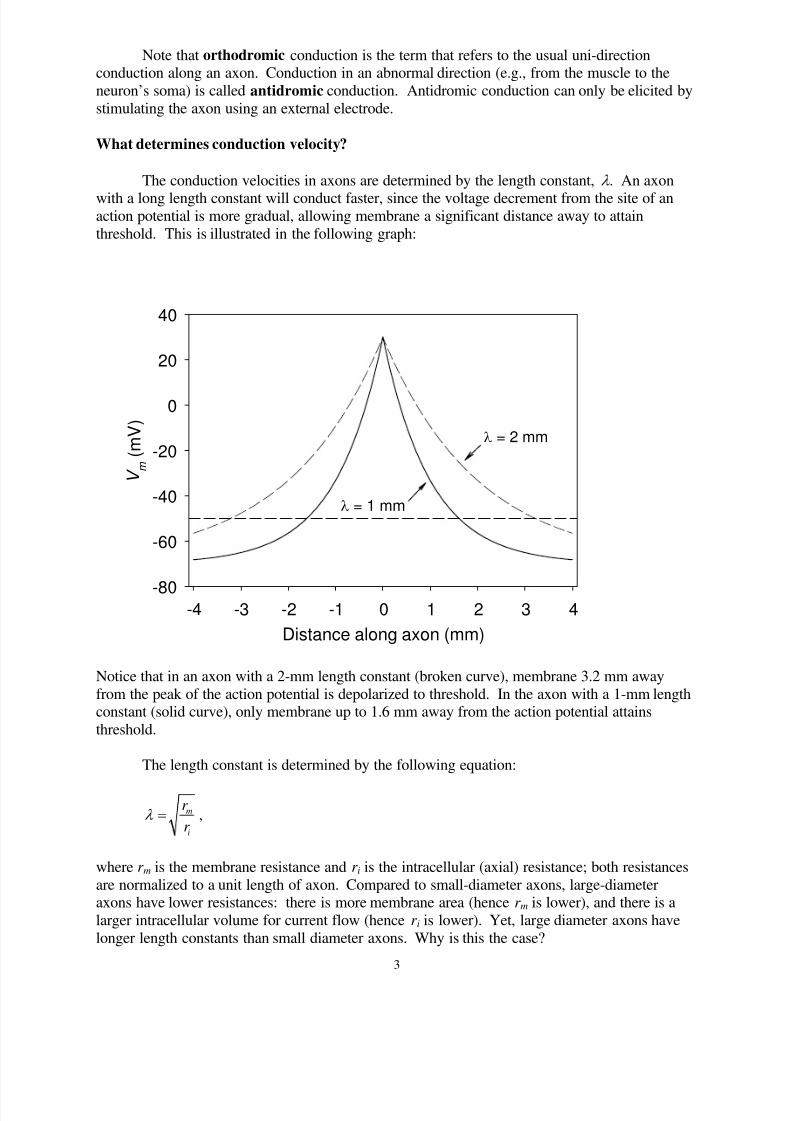
What determines conduction velocity?

The conduction velocities in axons are determined by the length constant, l . An axon

with a long length constant will conduct faster, since the voltage decrement from the site of anaction potential is more gradual, allowing membrane a significant distance away to attain

threshold. This is illustrated in the following graph:

Notice that in an axon with a 2-mm length constant (broken curve), membrane 3.2 mm away

from the peak of the action potential is depolarized to threshold. In the axon with a 1-mm lengthconstant (solid curve), only membrane up to 1.6 mm away from the action potential attains

threshold.

The length constant is determined by the following equation:

m

i

r

r l = ,

where r m is the membrane resistance and r i is the intracellular (axial) resistance; both resistances

are normalized to a unit length of axon. Compared to small-diameter axons, large-diameteraxons have lower resistances: there is more membrane area (hence r m is lower), and there is a

larger intracellular volume for current flow (hence r i is lower). Yet, large diameter axons have

longer length constants than small diameter axons. Why is this the case?

Distance along axon (mm)

-4 -3 -2 -1 0 1 2 3 4

V m

( m V )

-80

-60

-40

-20

0

20

40

l = 1 mm

l = 2 mm



4

The reason is that r m varies inversely with axon diameter, but r i varies inversely with the

square of axon diameter. Stated mathematically,

1mr

d µ and

2

1ir

d µ ,

where d is the axon diameter and µdenotes proportionality. Since with increasing diameter the

relative decrease in r m is less than the relative decrease in r i, / m ir r becomes larger, and thus l

( / m ir r = ) becomes larger as well.

So to reiterate… large-diameter axons conduct faster than small-diameter axons because

larg-diameter axons have longer length constants than small-diameter axons. Recall the studiesperformed using the squid giant axon—one of the largest diameter (1 mm) axon found in nature

(it was originally thought to be a vessel). Why is the squid giant axon so large? Recall also the

function of that axon: to cause contraction of the squid’s mantle thereby rapidly propelling theanimal out of harms way. It is in a squid’s best interest to have the conduction velocity of that

axon as fast as possible, such that the emergency escape reflex is as rapid as possible.

A major evolutionary advantage for vertebrates: myelin

Invertebrates can only achieve high conduction velocities solely by increasing (through

evolution) the diameter of their axons, but this comes with a price: having large-diameter axonslimits the number of high-speed axons in a given anatomical space. A major evolutionary

advantage occurred with the emergence of vertebrates, which permitted the packaging of literally

millions of high-speed axons in a small cross-sectional area (like that of the human spinal cord).

The strategy adopted by vertebrates was to increase l by effectively increasing r m, and

this is done by glial cells that surround axons. The glial cells wrap several layers of an insulating

material called myelin tightly around the axon (this is perfectly analogous to wrapping severallayers of electrical tape around a bare copper wire). The following diagram shows a cross

section of a so-called myelinated axon:

The concentric layers of myelin effectively increase r m and prevent electrotonic currentfrom flowing across the membrane. Thus, the current must flow axially down the length of the



5

axon until it finds a gap between successive glial cells. These gaps along the axon are located at

nodes of Ranvier, where the bare (unmyelinated) axon membrane is exposed to extracellular

fluid. This is shown in the following diagram:

The Na+ channels are located solely at the nodes of

Ranvier. When an action potential occurs at a given

node, the intracellular flow of electrotonic currentdepolarizes the membrane at the next node, which then

attains threshold and generates another action potential.

Thus, nerve conduction involves the generation of action potentials that “jump” from node to node. Thisdiscontinuous type of nerve conduction is termed

saltatory conduction.

Although the large increase in l brought about

by myelination results in a tremendous increase in

conduction velocity, still further speed ups are achievedby increasing axon diameter (thereby reducing r i).

Thus, the fastest axons in the body are large-diameter

myelinated axons—notably, motor neurons that

innervate skeletal muscles which are termed a motorneurons.

The graph on the following page shows typical conduction velocity as a function of neuron diameter in both myelinated and unmyelinated axons.

Multiple Sclerosis (MS)

MS is caused by scattered, discrete areas of

demyelination in different regions of the nervous

system. It is notable that the disease appears not

to affect the neurons themselves, other than

disrupting conduction of their axons. Individuals

suffering from MS typically experience recurrent

attacks that come and go seemingly randomly

over many years; a typical attack lasts several

weeks. Symptoms vary depending on the specific

locations of the demyelination. They include

impaired vision, loss of tactile sensations,

weakness or paralysis of the limbs, loss of

coordination, tremors, and other varied

symptoms.

The cause of MS is unknown, although some

evidence indicates that it may be an autoimmune

disorder whereby something goes awry with theimmune system, which then “attacks” the glial

cells.

There is no effective treatment of MS, although a

number of drugs are useful in ameliorating the

acute symptoms.



6

Notice that for unmyelinatedaxons, conduction velocity increases as

the square-root of the diameter (i.e., a

two-fold increase in diameter produces

only about a 2 1.4= -fold increase in

velocity). The conduction velocity of myelinated axons increases almost

linearly with diameter. But notice

something interesting, as seen in theinset of the figure. At very small axondiameters, unmyelinated axons actually

conduct faster than myelinated axons.

This is exploited by the body: smallneurons with axon diameters less than

»2 mm are unmyelinated, whereas

larger neurons are invariably always

found to be myelinated.

White matter versus gray matter

Myelin is a fatty substance (like “pig fat”) and is white in appearance. Neurons

composed of myelinated axons therefore appear white. Neurons lacking myelin appear gray.This has lead to the common differentiation of nervous tissue as being either white matter or

gray matter. When you see white matter, think of large myelinated high-speed axons that are

carrying information (nerve impulses) long distances. When you see gray matter, think of small-

diameter short neurons that are involved in processing the information.

Measuring neuron conduction velocities

In the laboratory, the conduction velocity of a neuron’s axon can be measured quite

simply by using two microelectrodes inserted into the axon at a known distance apart. This,however, is not feasible in the clinical setting. Neurologists measure the conduction velocity of,

say, the ulnar nerve of the arm, by measuring the so-called compound action potential.

Homework: Using the data in the above graph, estimate the

conduction velocity of an unmyelinated squid giant axon. Assume

that the diameter of the giant axon is 1 mm (1000 mm). (Answer:

about 90 m/sec.) Roughly how many mammalian axons of similarspeed could be placed within a 1 mm2 cross-sectional area (the

area occupied by one squid giant axon)? (Answer: about 400.)

Neuron Diameter (mm)

0 2 4 6 8 10 12

C o n d u c t i o n V e l o c i t y ( m / s e c )

0

20

40

60

80

100

mm0.0 0.4 0.8 1.2

m / s e c

0

2

4

6

8

Myelinated

Unmyelinated



7

The compound action potential differs from a neuron’s action potential in two ways.

First, it is an extracellular potential that does not reflect the axon’s true membrane potential.

And second, the compound action potential reflects the electrical response of the entire nerve.As such, it reflects the average response of all the neurons comprising the nerve.

The figure (above) shows how a compound action potential is recorded. The gray tube

depicts a nerve comprising a number of different axons (small ovals). A differential voltmeter

is attached to two electrodes placed on the skin (black rectangles). The voltmeter measures the

difference in the voltage between the two electrodes; if the left electrode is at a potential negative

to that of the right electrode, then a negative deflection will appear on the meter (and vice versa).Now, assume action potentials were elicited in the nerve axons at time t = 0 msec by stimulating

the nerve with an electric shock at the point indicated by the black arrow; also assume that this

triggers a recording device (typically an oscilloscope or a personal computer) that starts to plotthe meter’s voltage as a function of time (graph).

As the action potentials propagate down the nerve axons (white arrow), the extracellular

voltage starts off positive at rest (+’s on the right of the figure), briefly becomes negative where

the action potentials are occurring (-’s in the center of the figure), and returns to positive values

after the nerve axons repolarize (+’s on the left of the figure). This is due to the electrotonic

currents that flow across the axons and through the extracellular solution as the action potential

conducts. But, prior to the arrival of action potentials at the recording (skin) electrodes, thevoltmeter will record no voltage change, since the two electrodes are over regions measuring the

same potential (recall, the voltmeter measures the difference in the voltage between the twoelectrodes). This is depicted as no potential change in the recording (horizontal black line at

0 mV).

As the action potentials propagate under the recording electrodes (above), one starts toobserve a voltage difference. Namely, the left electrode is over the region of depolarized axons

while the right electrode is over a region of resting axons. This produces the negative deflection

shown in the graph. Notice, however, the size of the deflection—it is only a few microvolts

(mV) in amplitude, not the tens-of-millivolts typical of an action potential! The voltage simply

timemV

timemV



8

reflects the small extracellular currents flowing through the low resistance extracellular fluid

(i.e., by Ohm’s Law, eV ir D = ).

As the action potentials continue to propagate, the voltages under the electrodes briefly

reverse polarity (see above), where the right electrode measures the voltage of the depolarizedaxons, while the left electrode measures the voltage adjacent to repolarized axons.

Finally, after the action potentials have conducted past the recording electrodes, the measured

voltage returns to zero, reflecting the fact that the entire nerve has repolarized (or returned to

resting), thereby producing the characteristic biphasic tracing seen in the graph. The conductionvelocity of the compound action potential is computed by simply dividing the distance between

the stimulation electrode (black arrow in first figure, above) by the time of the first deflectionseen in the tracing.

The figure on the right shows the

actual setup for measuring nerve conduction

in the hand, in this case, to aid in thediagnosis of carpal tunnel syndrome (a

syndrome resulting in poor nerve conduction

in the wrist). The recording electrodes aretaped on the skin at the base of the thumb.

The two-pointed device placed over the wrist

is the stimulating electrode—a device(similar to a Taser®) that delivers a high-

voltage, but brief, shock, thereby eliciting

action potentials in the underlying nerves. When the clinician triggers the shock (switch on

stimulating electrode), this triggers the collection (by a personal computer) of the voltagesmeasured by the recording electrodes as a function of time.

timemV

time

mV



9

The figure on the next page shows an

actual recording displayed on the computer’s

monitor. In this example, the recording wasdone from recording electrodes placed over the

ulnar nerve at the wrist, with the stimulating

electrode positioned at the upper forearm.

Disregard the voltage scale, which shows

units of volts! It reflects the gain of an

amplifier (typically >1000) needed to amplifythe tiny extracellular voltage to levels suitablefor the computer.

The initial brief voltage deflection (seenat 0 msec) is the so-called stimulus artifact—a

signal produced by the stimulus electrode and conducted to the recording electrodes by the

resistive properties of the skin. The stimulus artifact does not reflect nerve conduction (albeit, it

does provide a useful index of when the stimulus was applied). The dark region of the tracingindicates the time period (4.6 msec) for the arrival of action potentials at the recording electrode.

In this example, the distance between the stimulus and recording electrodes was 30 cm, resulting

in a ulnar nerve conduction velocity of 0.3 m/0.0046 sec = 65 m/sec (a typical value).

But, notice something “odd” in the recording. The first deflection in voltage occurs at

4.6 msec, yet the compound action potential is >15 msec in duration. Aren’t action potentials

rapid events, with duration of 1-2 msec? The resolution of this apparent paradox is obviouswhen one remembers the fact that compound action potentials reflect the response in an entire

nerve as opposed to a single neuron. The nerve contains the axons of thousands of different

neurons, with differing conduction velocities. All these axons are being stimulatedsimultaneously, with the fastest conducting action potentials arriving at the recording electrodes

at 4.6 msec, but others taking substantially longer. This results in the somewhat complicated

(“bumpy”) waveform seen in the figure, with a duration far longer than that of a single action

potential.

What is the clinical utility of measuring a compound action potential? The progression of

(or recovery from) demyelinating diseases like multiple sclerosis and ALS (amyotrophic lateralsclerosis, or Lou Gehrig’s disease) can be monitored by monitoring nerve conduction velocity,

since demyelination causes a reduction in conduction velocity. Also, the anatomical site of a

nerve injury can often be precisely located by measuring a compound action potential. This isdone by positioning the recording electrodes at, say, the site of a denervated (paralyzed) muscle,

then positioning the stimulating electrode at different distances along the nerve looking for the

point at which it is capable of eliciting a compound action potential—i.e., at distances along thenerve just distal to the injury. And, the total amplitude of the compound action potential is

useful in assessing reinnervation of peripheral nerves following a nerve injury. Since theamplitude is proportional to the number of conducting axons within the nerve, the neurologistcan follow the gradual reinnervation process as more and more of the nerve’s axons start to

conduct.

action potential conduction

Documents