accelerometers: one size does not fit all
TRANSCRIPT
Accelerometers:One size does not fit all…Jeremy DailyJohn Daily20th Annual IATAI Conference 6-8 Sept 2006PA. State Police Reconstruction Conference 27 Sept 2006
Overview
Identify the need for accelerometersSurvey of accelerometer typesOverall measurement system
Sensors TransducersSignal ConditionersOutput
Accelerometer systemsSpecifications for measuring acceleration
Range, Resolution, and Frequency
Why use an accelerometer?
Need drag factor for speed computationsOnly technique capable of measuring truly representative valuesAccounts for total vehicle/braking/tire/road systemShould use an exemplar vehicle on site if possible
Measure straight line acceleration
What else?
Lateral Acceleration in Yaw testingCrash Testing and Sensing
Air bag deploymentNCAP, J211, Government sponsored crash testingCrash test dummiesDetermine PDOF during crashPost impact trajectory
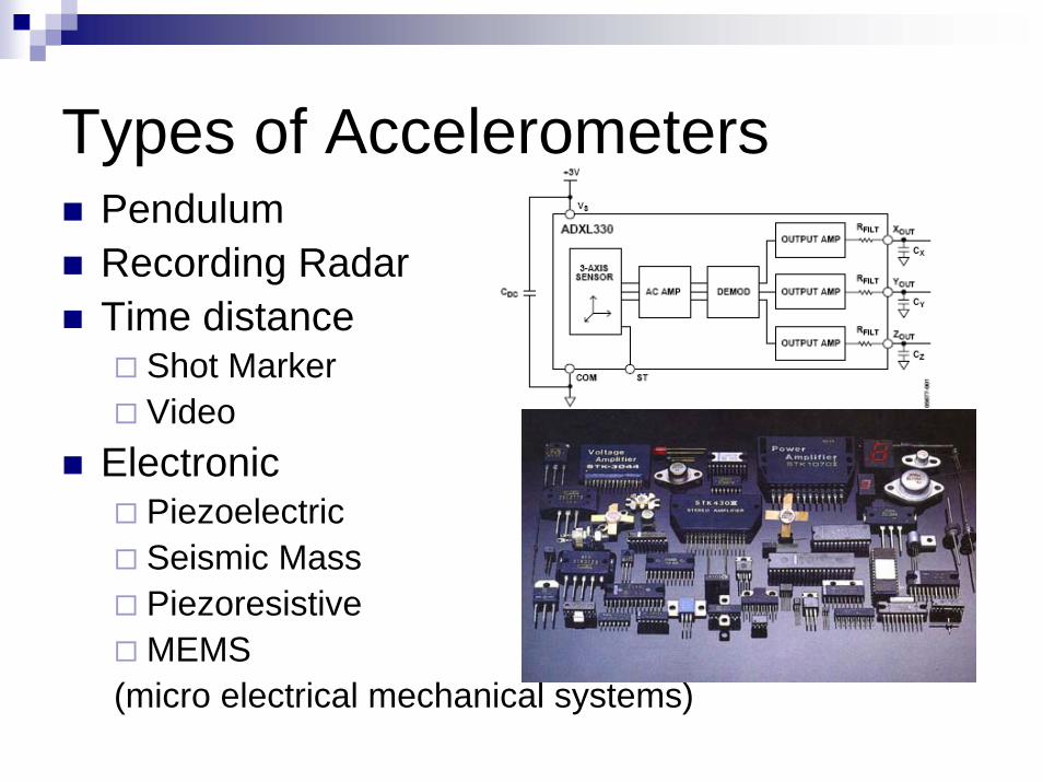
Types of AccelerometersPendulum Recording RadarTime distance
Shot MarkerVideo
ElectronicPiezoelectricSeismic Mass PiezoresistiveMEMS
(micro electrical mechanical systems)
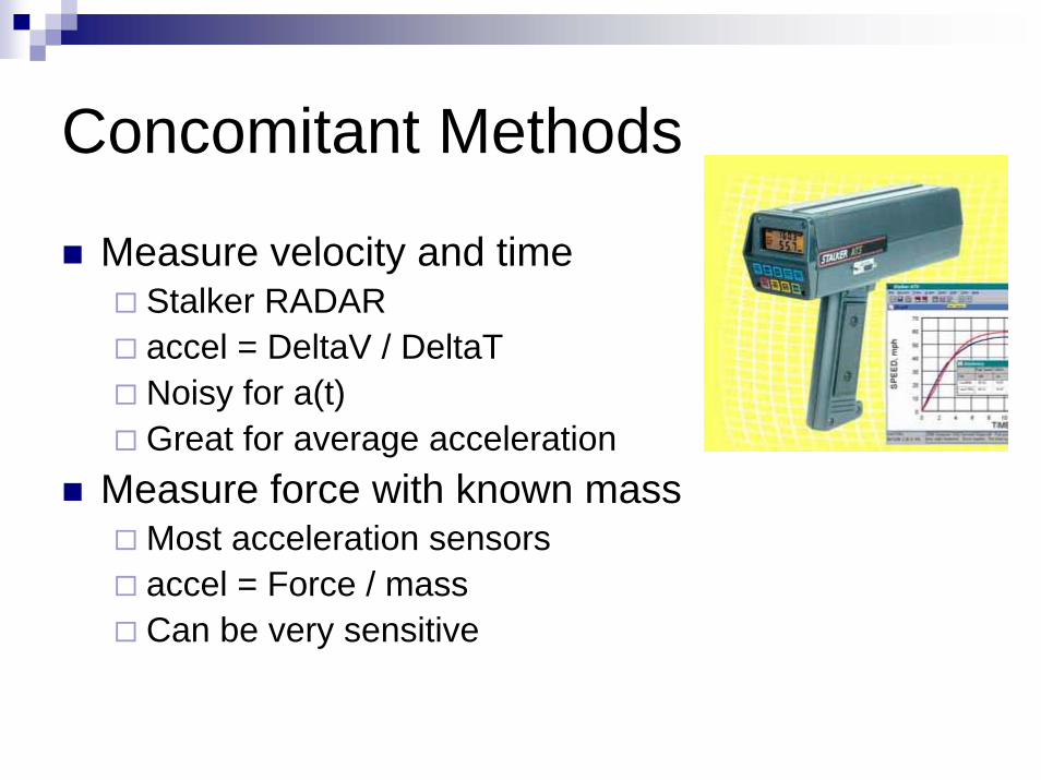
Concomitant Methods
Measure velocity and timeStalker RADARaccel = DeltaV / DeltaTNoisy for a(t)Great for average acceleration
Measure force with known massMost acceleration sensorsaccel = Force / massCan be very sensitive
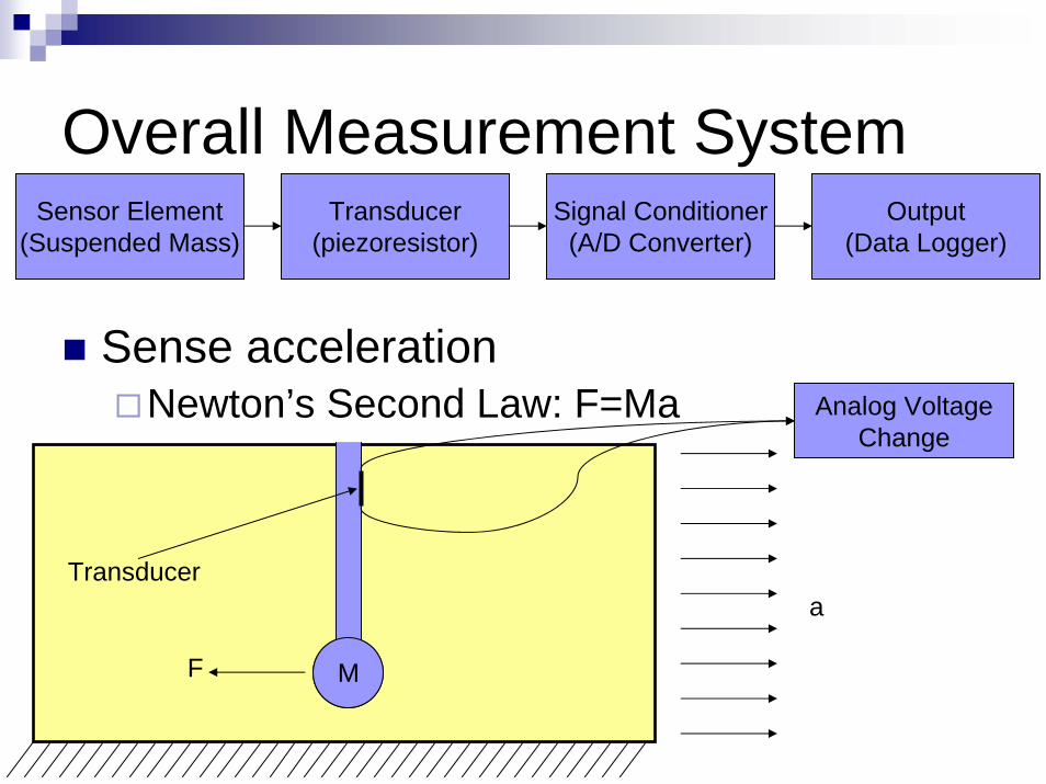
Overall Measurement SystemSensor Element
(Suspended Mass)Transducer
(piezoresistor)Signal Conditioner
(A/D Converter)Output
(Data Logger)
MM
Sense accelerationNewton’s Second Law: F=Ma Analog Voltage
Change
F
aTransducer
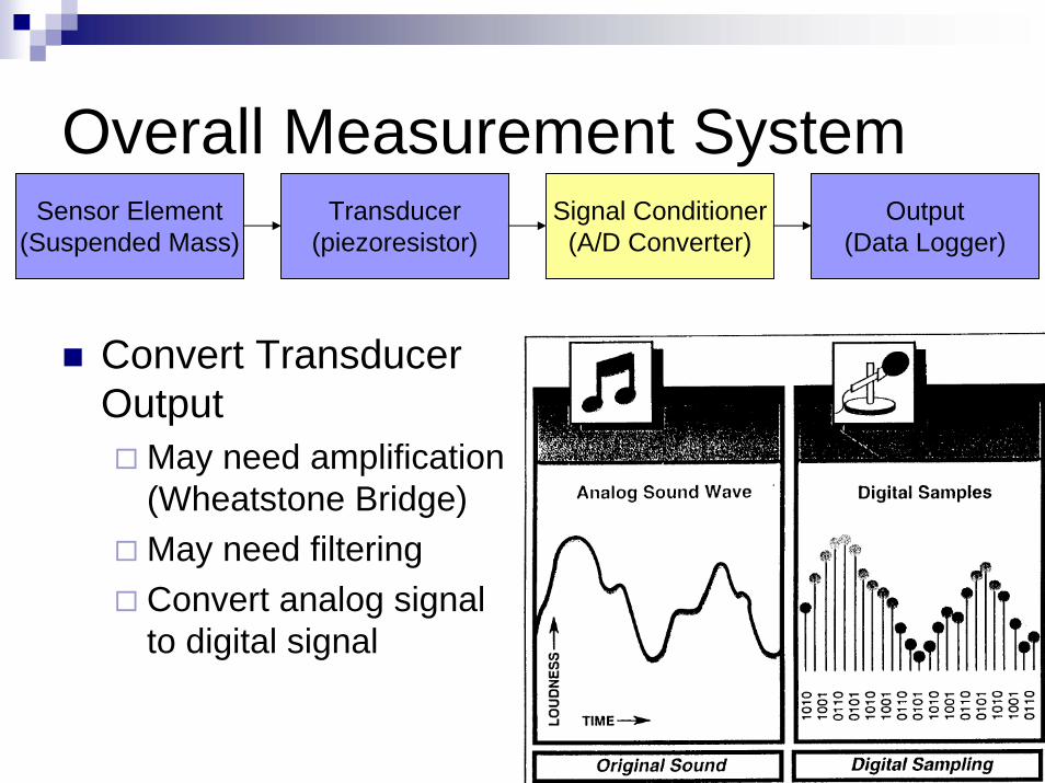
Overall Measurement System
Convert Transducer Output
May need amplification (Wheatstone Bridge)May need filteringConvert analog signal to digital signal
Sensor Element(Suspended Mass)
Transducer(piezoresistor)
Signal Conditioner(A/D Converter)
Output(Data Logger)
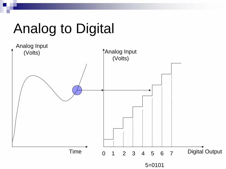
Analog to Digital
0 1 2 3 4 5 6 7
5=0101
Digital Output
Analog Input (Volts)
Analog Input (Volts)
Time
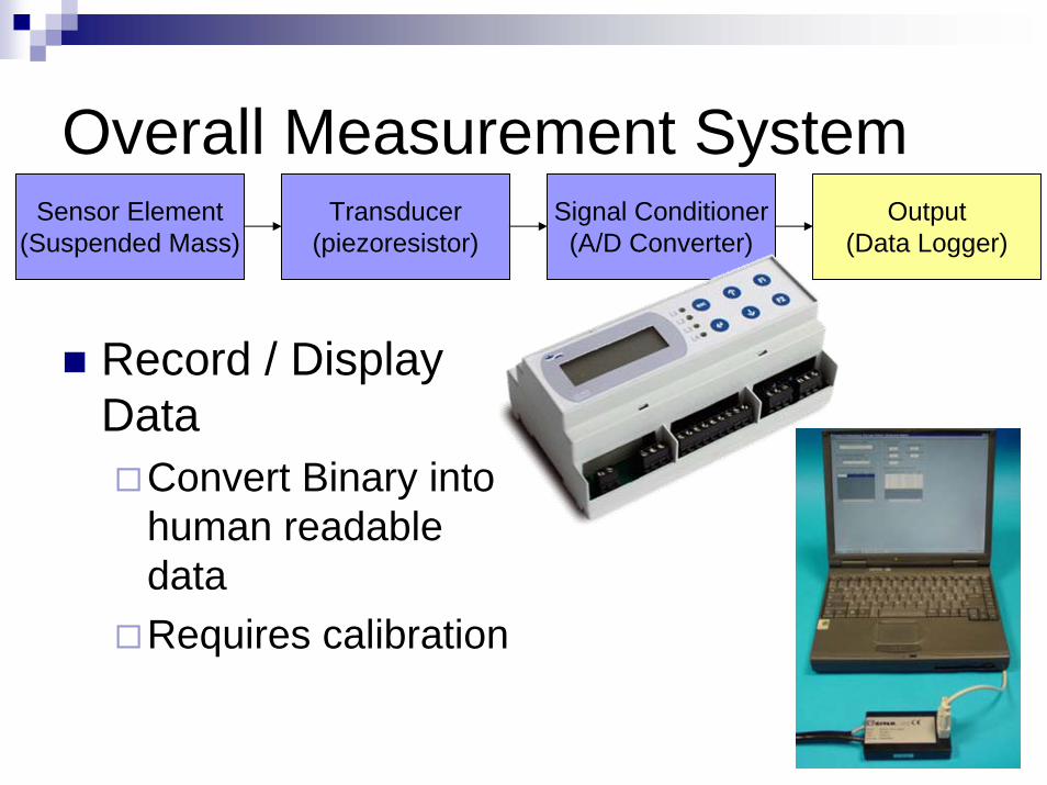
Overall Measurement System
Record / Display Data
Convert Binary into human readable dataRequires calibration
Sensor Element(Suspended Mass)
Transducer(piezoresistor)
Signal Conditioner(A/D Converter)
Output(Data Logger)
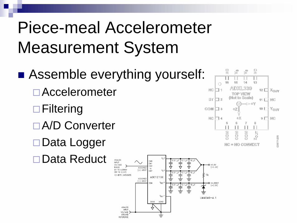
Piece-meal Accelerometer Measurement System
Assemble everything yourself:AccelerometerFilteringA/D ConverterData LoggerData Reduction/Interpretation
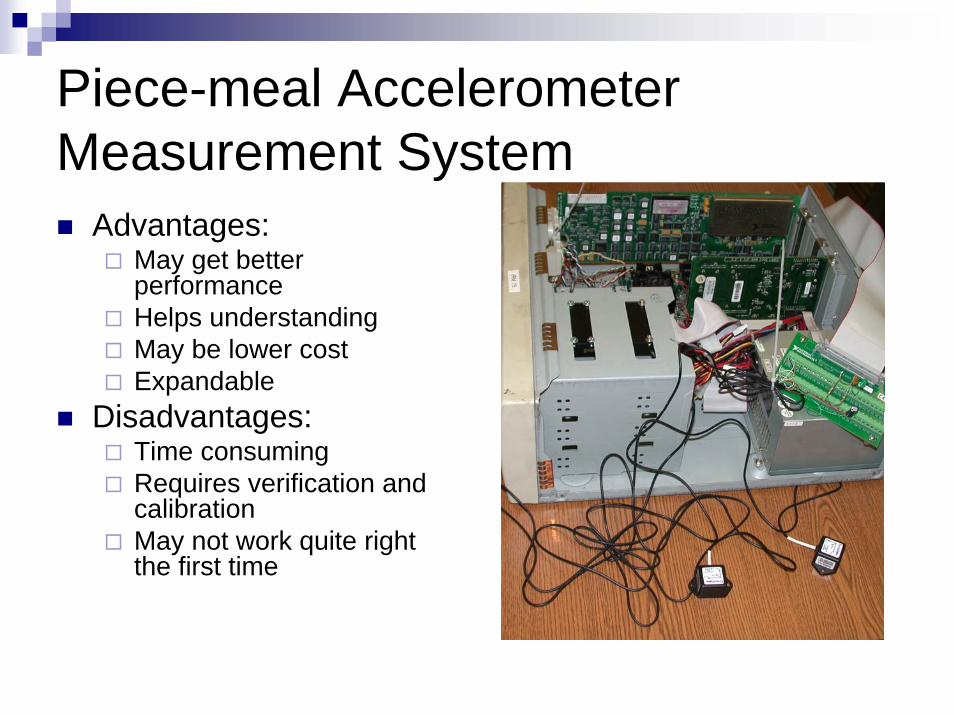
Piece-meal Accelerometer Measurement System
Advantages:May get better performanceHelps understandingMay be lower costExpandable
Disadvantages:Time consumingRequires verification and calibrationMay not work quite right the first time
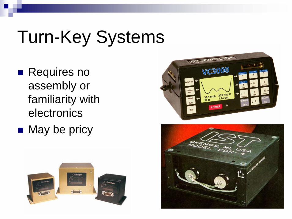
Turn-Key Systems
Requires no assembly or familiarity with electronicsMay be pricy
Comparing Accelerometer Systems
RangeWhat is the anticipated range (Peak-Peak) of the event?
+/- 1.5 G for braking/acceleration+/- 100G (possibly) for crash events
Sampling FrequencyHow long does your event last?
a.k.a: PeriodAre there details within your event?How much memory (cost) can you afford?Are there frequency limits for the sensor?
DC coupled/output (good for vehicle performance)High frequency capabilities (good for crash testing)
Comparing Accelerometer Systems
ResolutionHow many bits does your Analog to Digital Converter use?Number of levels = 2# of bits
e.g. 10 bits gives 210 = 1024 possible valuese.g. 12 bits gives 212 = 4096 possible values
Resolution is the range of the instrument divided by the number of levels
n
rangeres2
=
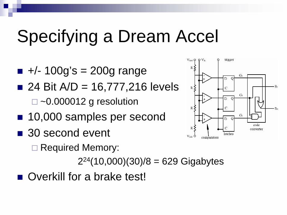
Specifying a Dream Accel
+/- 100g’s = 200g range24 Bit A/D = 16,777,216 levels
~0.000012 g resolution10,000 samples per second30 second event
Required Memory: 224(10,000)(30)/8 = 629 Gigabytes
Overkill for a brake test!
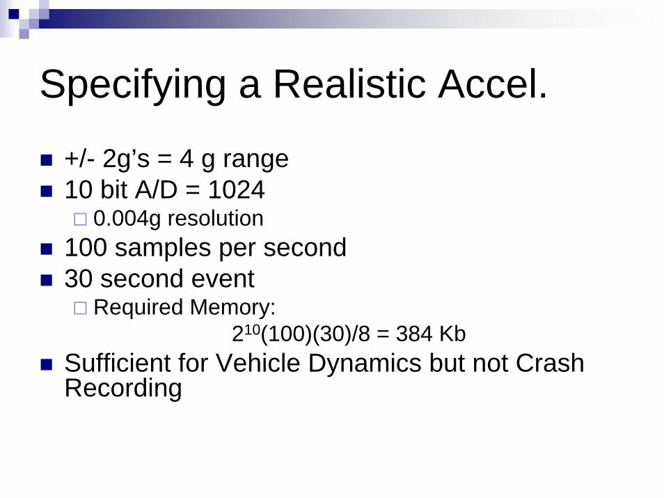
Specifying a Realistic Accel.
+/- 2g’s = 4 g range10 bit A/D = 1024
0.004g resolution100 samples per second30 second event
Required Memory: 210(100)(30)/8 = 384 Kb
Sufficient for Vehicle Dynamics but not Crash Recording
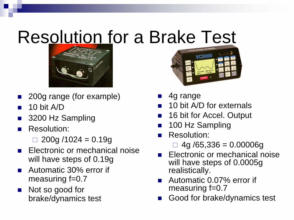
Resolution for a Brake Test
200g range (for example)10 bit A/D3200 Hz SamplingResolution:
200g /1024 = 0.19gElectronic or mechanical noise will have steps of 0.19gAutomatic 30% error if measuring f=0.7Not so good for brake/dynamics test
4g range10 bit A/D for externals16 bit for Accel. Output100 Hz SamplingResolution:
4g /65,336 = 0.00006gElectronic or mechanical noise will have steps of 0.0005g realistically.Automatic 0.07% error if measuring f=0.7Good for brake/dynamics test
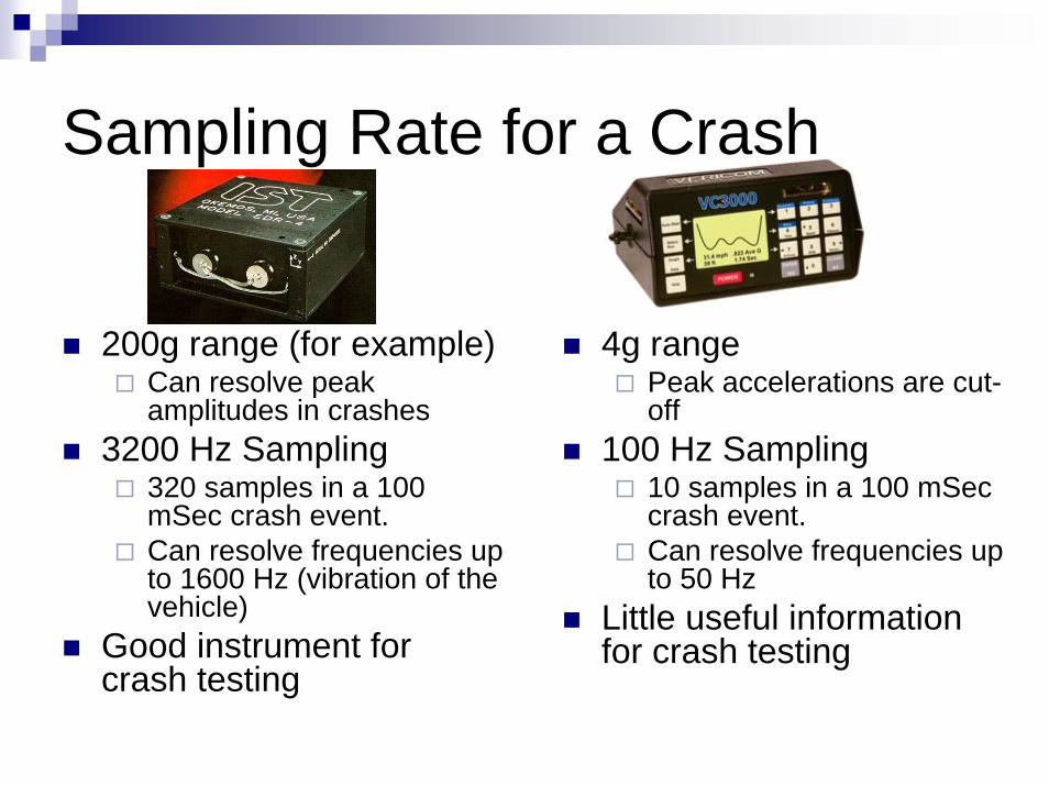
Sampling Rate for a Crash
200g range (for example)Can resolve peak amplitudes in crashes
3200 Hz Sampling320 samples in a 100 mSec crash event.Can resolve frequencies up to 1600 Hz (vibration of the vehicle)
Good instrument for crash testing
4g rangePeak accelerations are cut-off
100 Hz Sampling10 samples in a 100 mSeccrash event.Can resolve frequencies up to 50 Hz
Little useful information for crash testing
Common Mistakes
Reporting only peak valuesCommon in popular literature
Be wary of “misapplying” accelerometer results
Crown Vic with Eagle RS-A may not represent a Geo MetroNew F-150 may not represent old Chevy ¾ton.
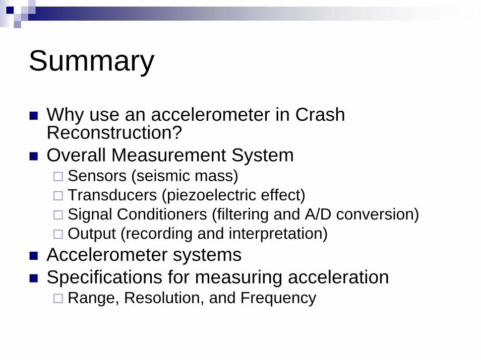
Summary
Why use an accelerometer in Crash Reconstruction?Overall Measurement System
Sensors (seismic mass)Transducers (piezoelectric effect)Signal Conditioners (filtering and A/D conversion)Output (recording and interpretation)
Accelerometer systemsSpecifications for measuring acceleration
Range, Resolution, and Frequency
Using Accelerometer Data
What do we do with the information?
What are we going to do?
First of all, we will examine various ways of starting the VC3000DAQ accelerometer.Next, we will look at the data generated during the accelerometer runs.We will look at how to read and interpret the accelerometer graphs.We will summarize the results.
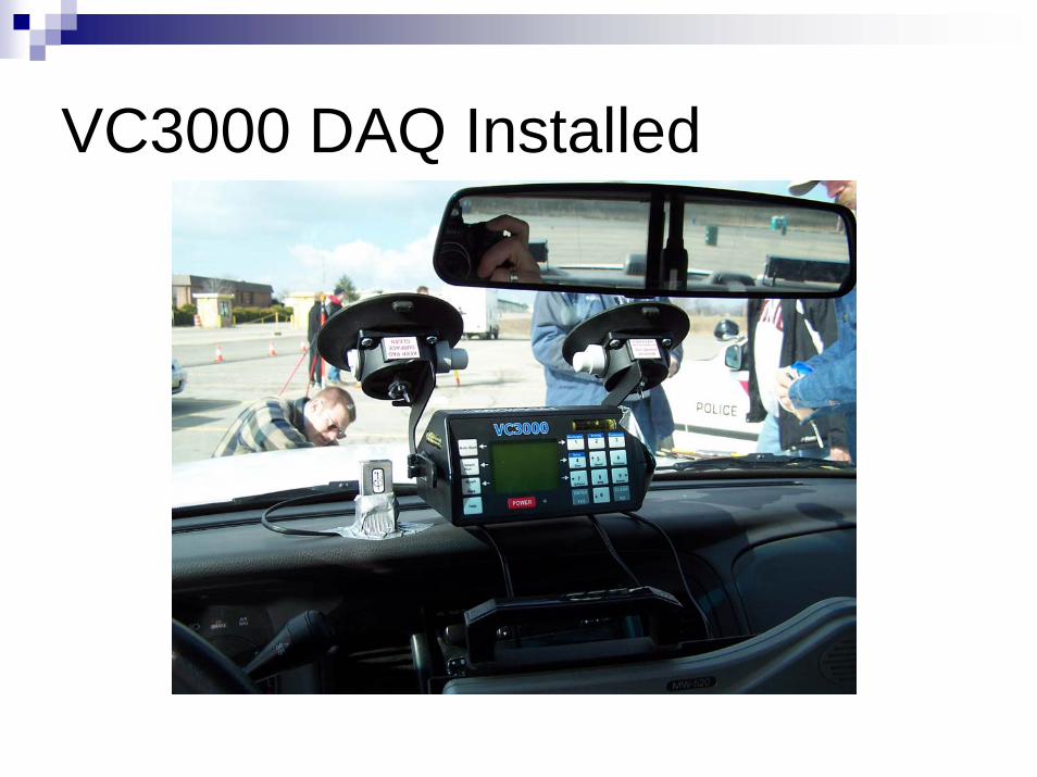
VC3000 DAQ Installed
Start Modes
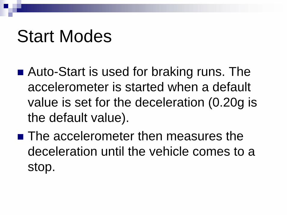
Auto-Start is used for braking runs. The accelerometer is started when a default value is set for the deceleration (0.20g is the default value).The accelerometer then measures the deceleration until the vehicle comes to a stop.
Start Modes
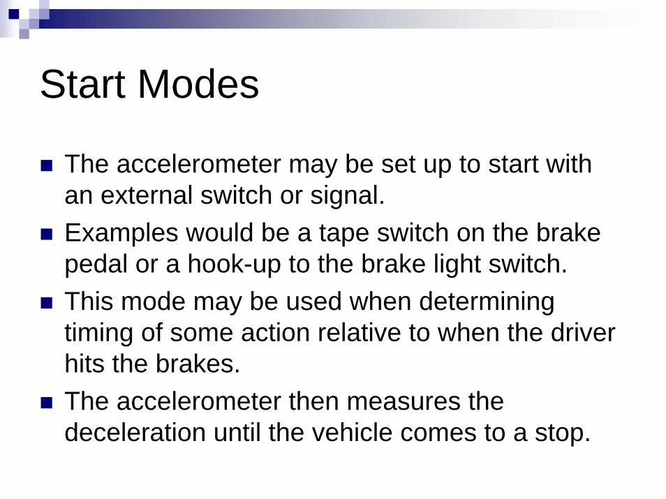
The accelerometer may be set up to start with an external switch or signal. Examples would be a tape switch on the brake pedal or a hook-up to the brake light switch.This mode may be used when determining timing of some action relative to when the driver hits the brakes.The accelerometer then measures the deceleration until the vehicle comes to a stop.
Start Modes
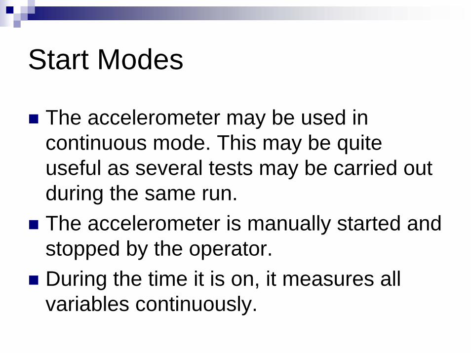
The accelerometer may be used in continuous mode. This may be quite useful as several tests may be carried out during the same run.The accelerometer is manually started and stopped by the operator.During the time it is on, it measures all variables continuously.
Auto-Start Braking Run
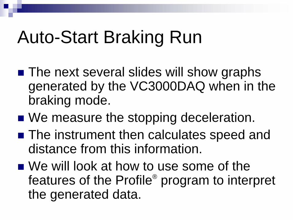
The next several slides will show graphs generated by the VC3000DAQ when in the braking mode. We measure the stopping deceleration.The instrument then calculates speed and distance from this information.We will look at how to use some of the features of the Profile® program to interpret the generated data.
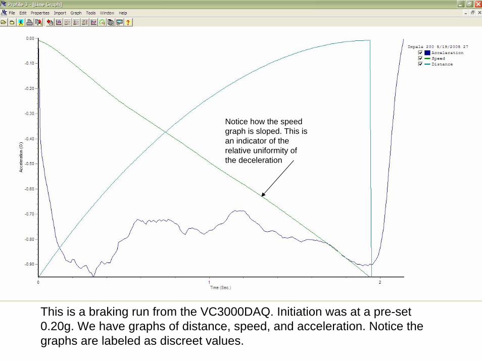
This is a braking run from the VC3000DAQ. Initiation was at a pre-set 0.20g. We have graphs of distance, speed, and acceleration. Notice the graphs are labeled as discreet values.
Notice how the speed graph is sloped. This is an indicator of the relative uniformity of the deceleration
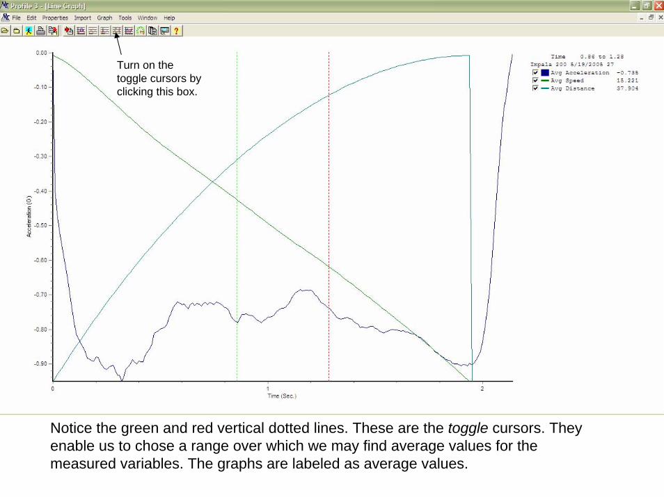
Notice the green and red vertical dotted lines. These are the toggle cursors. They enable us to chose a range over which we may find average values for the measured variables. The graphs are labeled as average values.
Turn on the toggle cursors by clicking this box.
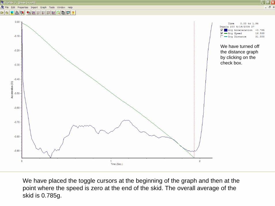
We have placed the toggle cursors at the beginning of the graph and then at the point where the speed is zero at the end of the skid. The overall average of the skid is 0.785g.
We have turned off the distance graph by clicking on the check box.
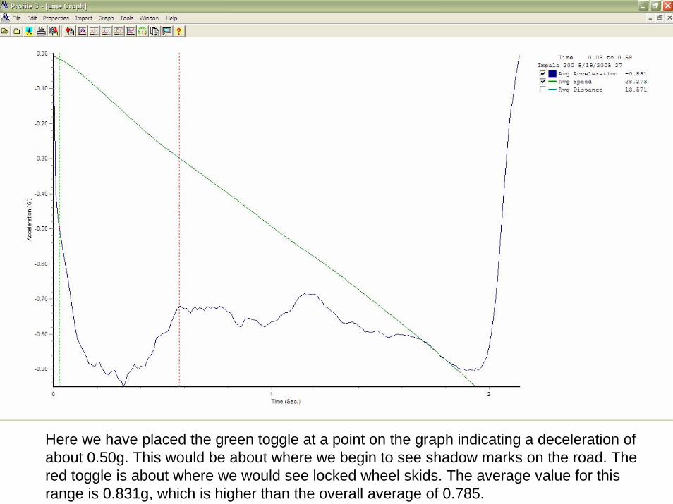
Here we have placed the green toggle at a point on the graph indicating a deceleration of about 0.50g. This would be about where we begin to see shadow marks on the road. The red toggle is about where we would see locked wheel skids. The average value for this range is 0.831g, which is higher than the overall average of 0.785.
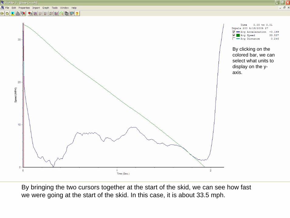
By clicking on the colored bar, we can select what units to display on the y-axis.
By bringing the two cursors together at the start of the skid, we can see how fast we were going at the start of the skid. In this case, it is about 33.5 mph.
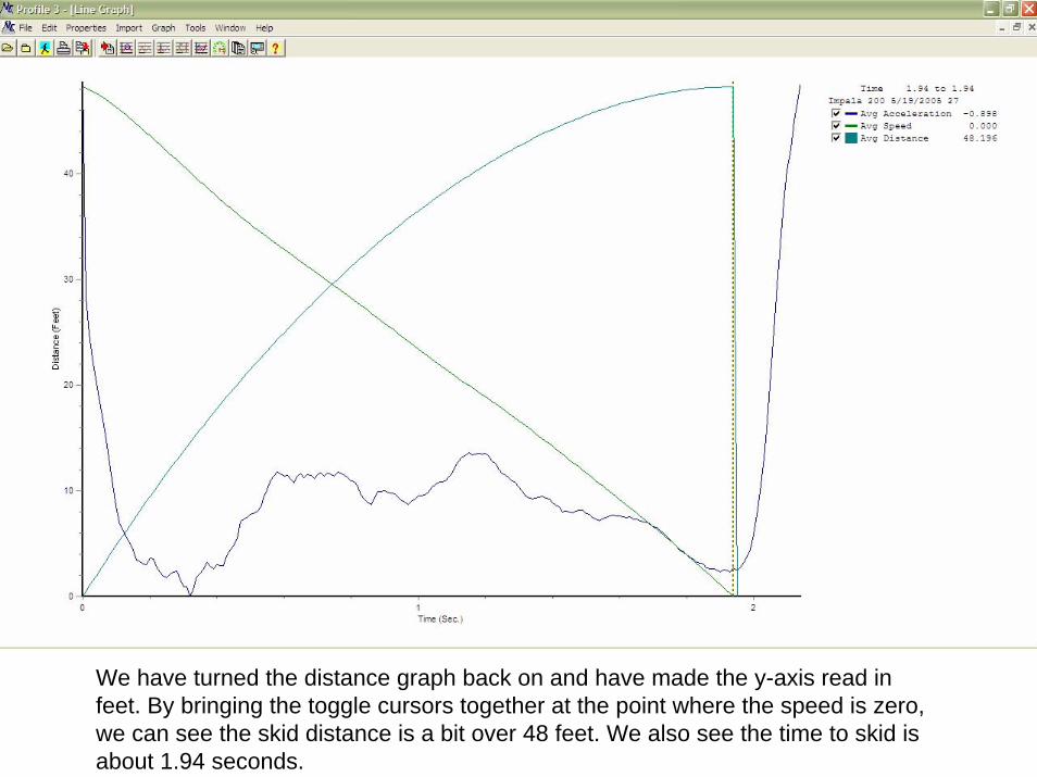
We have turned the distance graph back on and have made the y-axis read in feet. By bringing the toggle cursors together at the point where the speed is zero, we can see the skid distance is a bit over 48 feet. We also see the time to skid is about 1.94 seconds.
Discreet Start (Tape Switch)
This next set of slides will help us explore graphs generated by a discreet start.In this case, a tape switch on the brake
pedal will be used to start the instrument.In addition, an external pressure sensor will be plugged into the VC3000DAQ in order to measure the air pressure at the glad hands on a TT unit.
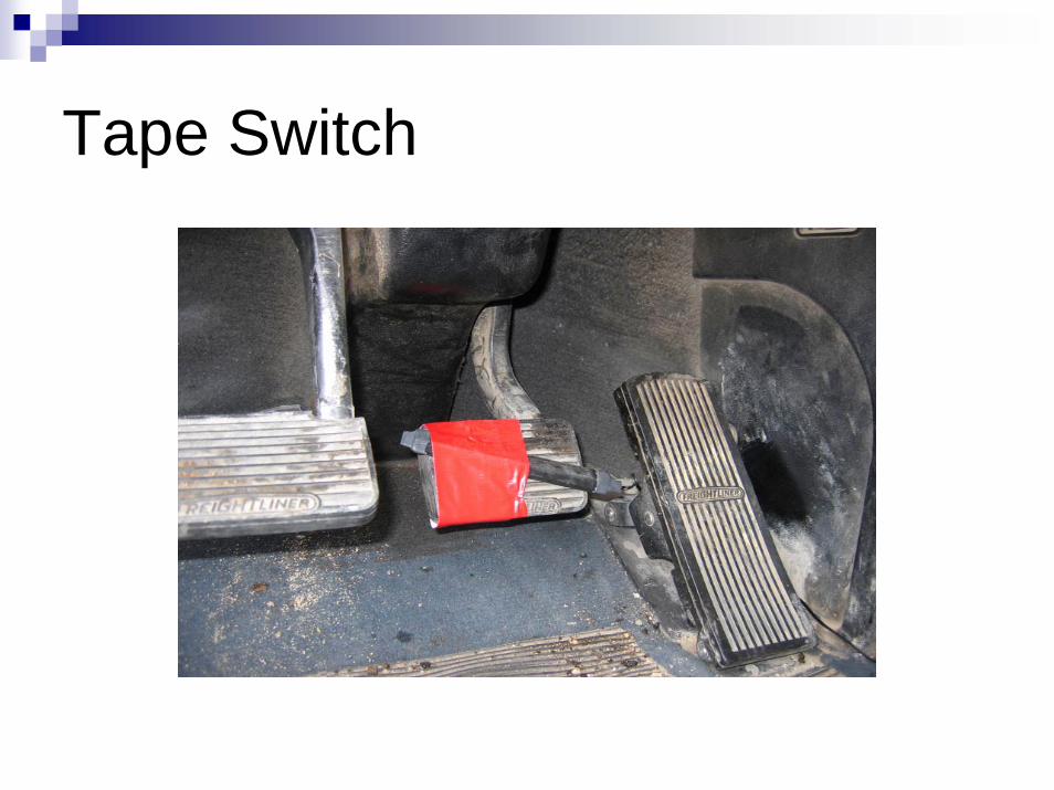
Tape Switch
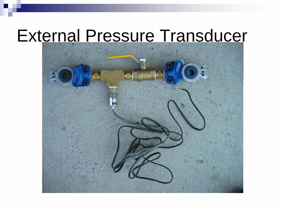
External Pressure Transducer
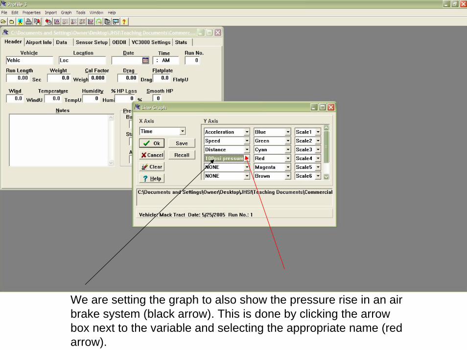
We are setting the graph to also show the pressure rise in an air brake system (black arrow). This is done by clicking the arrow box next to the variable and selecting the appropriate name (redarrow).
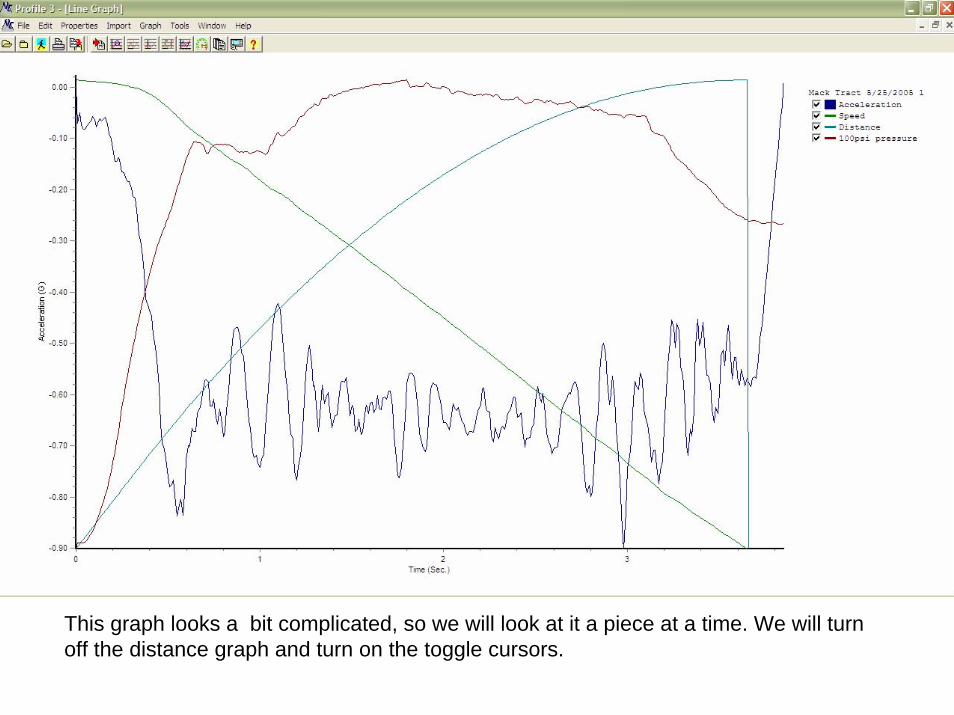
This graph looks a bit complicated, so we will look at it a piece at a time. We will turn off the distance graph and turn on the toggle cursors.
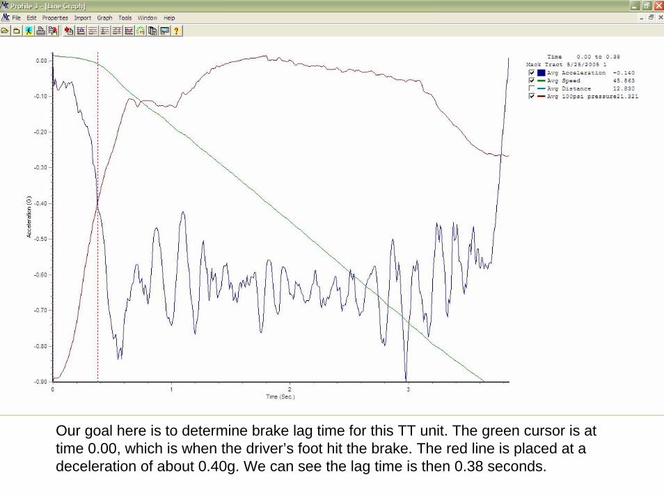
Our goal here is to determine brake lag time for this TT unit. The green cursor is at time 0.00, which is when the driver’s foot hit the brake. The red line is placed at a deceleration of about 0.40g. We can see the lag time is then 0.38 seconds.
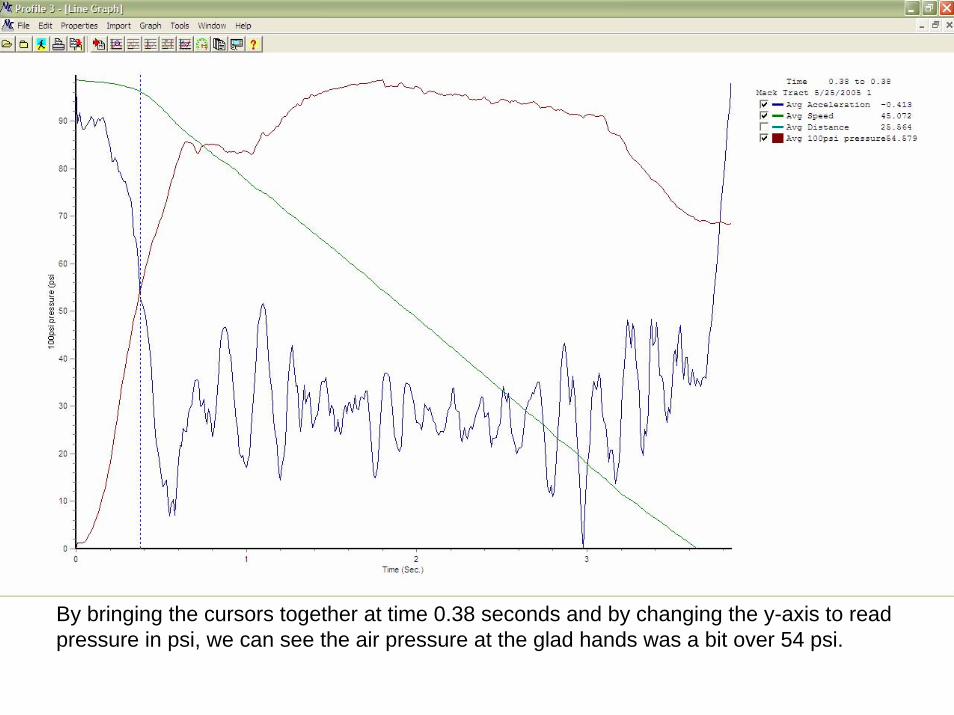
By bringing the cursors together at time 0.38 seconds and by changing the y-axis to read pressure in psi, we can see the air pressure at the glad hands was a bit over 54 psi.
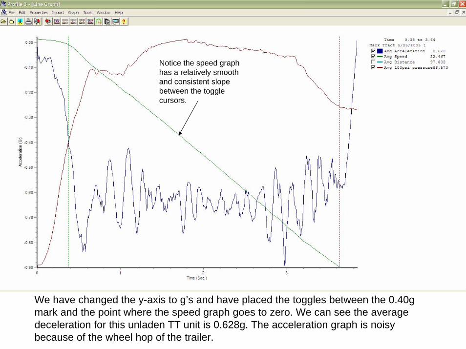
Notice the speed graph has a relatively smooth and consistent slope between the toggle cursors.
We have changed the y-axis to g’s and have placed the toggles between the 0.40g mark and the point where the speed graph goes to zero. We can see the average deceleration for this unladen TT unit is 0.628g. The acceleration graph is noisy because of the wheel hop of the trailer.
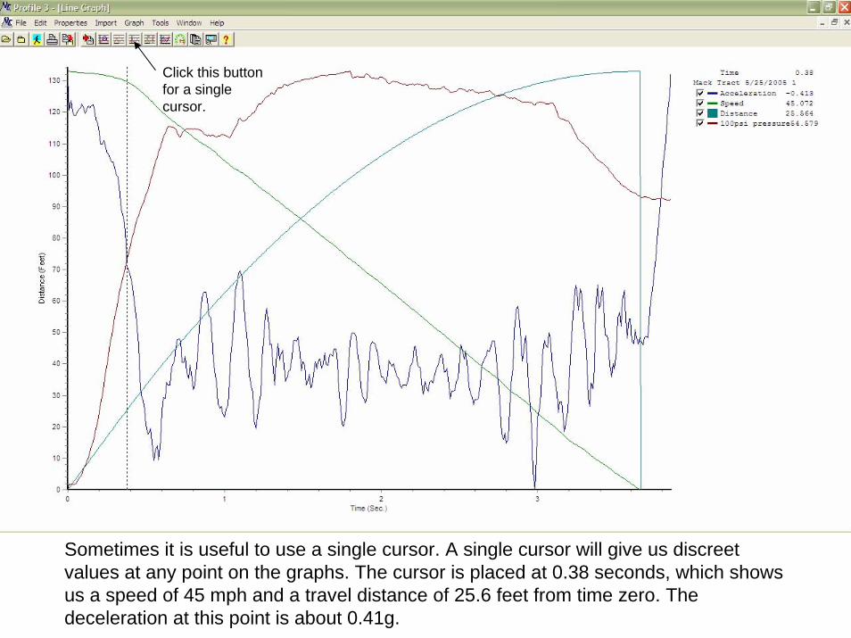
Click this button for a single cursor.
Sometimes it is useful to use a single cursor. A single cursor will give us discreet values at any point on the graphs. The cursor is placed at 0.38 seconds, which shows us a speed of 45 mph and a travel distance of 25.6 feet from time zero. The deceleration at this point is about 0.41g.
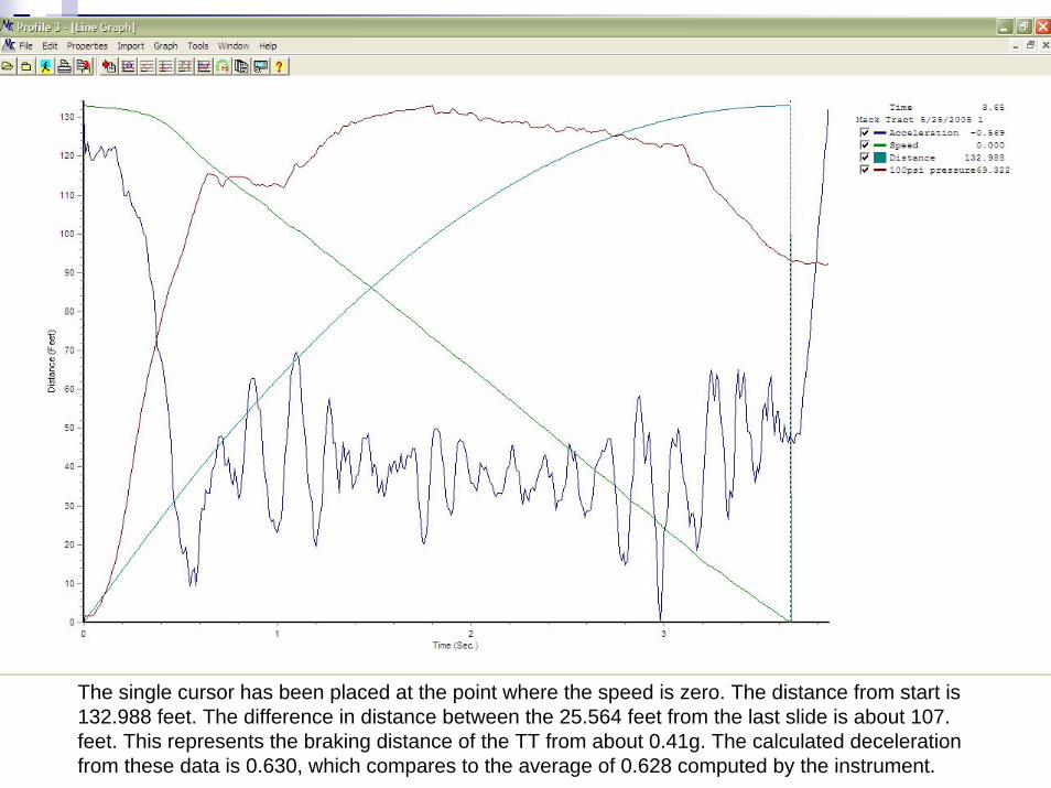
The single cursor has been placed at the point where the speed is zero. The distance from start is 132.988 feet. The difference in distance between the 25.564 feet from the last slide is about 107. feet. This represents the braking distance of the TT from about 0.41g. The calculated deceleration from these data is 0.630, which compares to the average of 0.628 computed by the instrument.
Continuous Mode
The continuous mode configuration allows measurement from the time the operator turns on the instrument until the instrument is turned off by the operator.This allows several performance variables to be measured in the same test, such as acceleration and braking.Lateral and longitudinal accelerations are measured simultaneously. Simultaneous data from other sensors may be gathered at the same time.
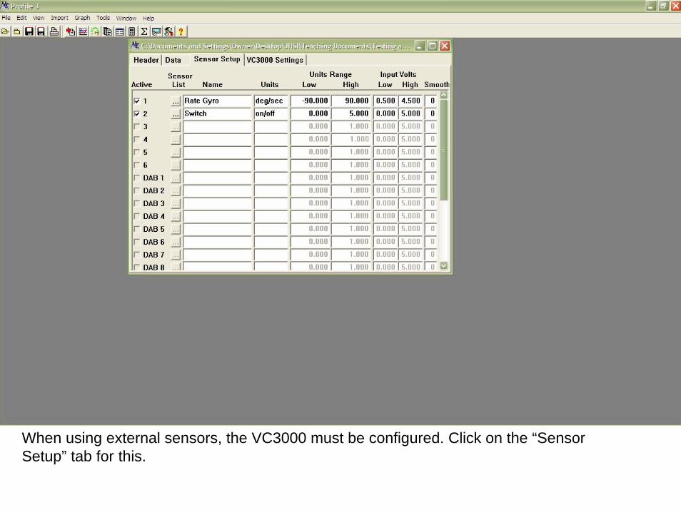
When using external sensors, the VC3000 must be configured. Click on the “Sensor Setup” tab for this.
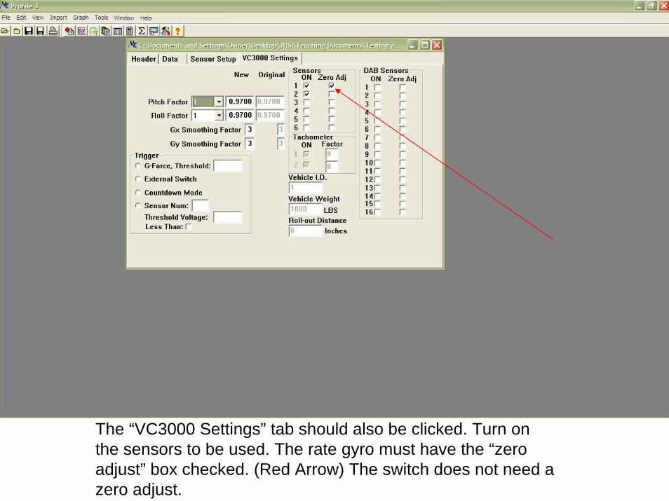
The “VC3000 Settings” tab should also be clicked. Turn on the sensors to be used. The rate gyro must have the “zero adjust” box checked. (Red Arrow) The switch does not need a zero adjust.
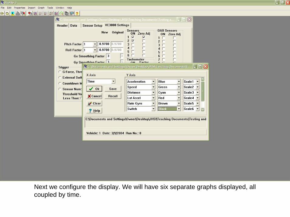
Next we configure the display. We will have six separate graphs displayed, all coupled by time.
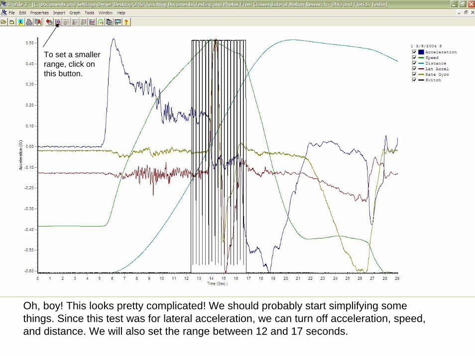
To set a smaller range, click on this button.
Oh, boy! This looks pretty complicated! We should probably start simplifying some things. Since this test was for lateral acceleration, we can turn off acceleration, speed, and distance. We will also set the range between 12 and 17 seconds.
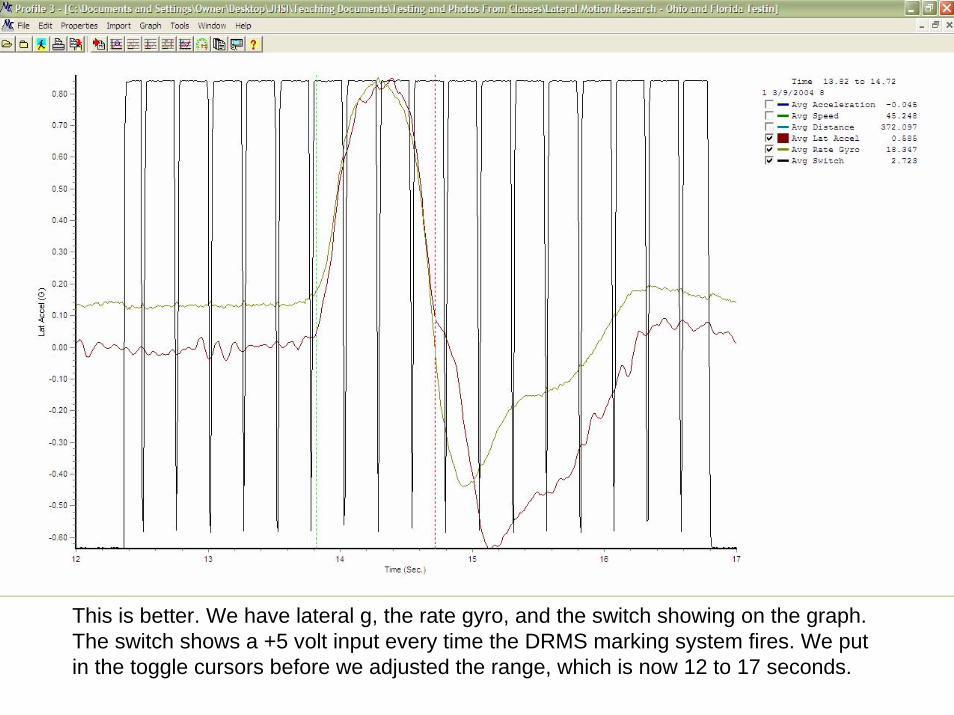
This is better. We have lateral g, the rate gyro, and the switch showing on the graph. The switch shows a +5 volt input every time the DRMS marking system fires. We put in the toggle cursors before we adjusted the range, which is now 12 to 17 seconds.
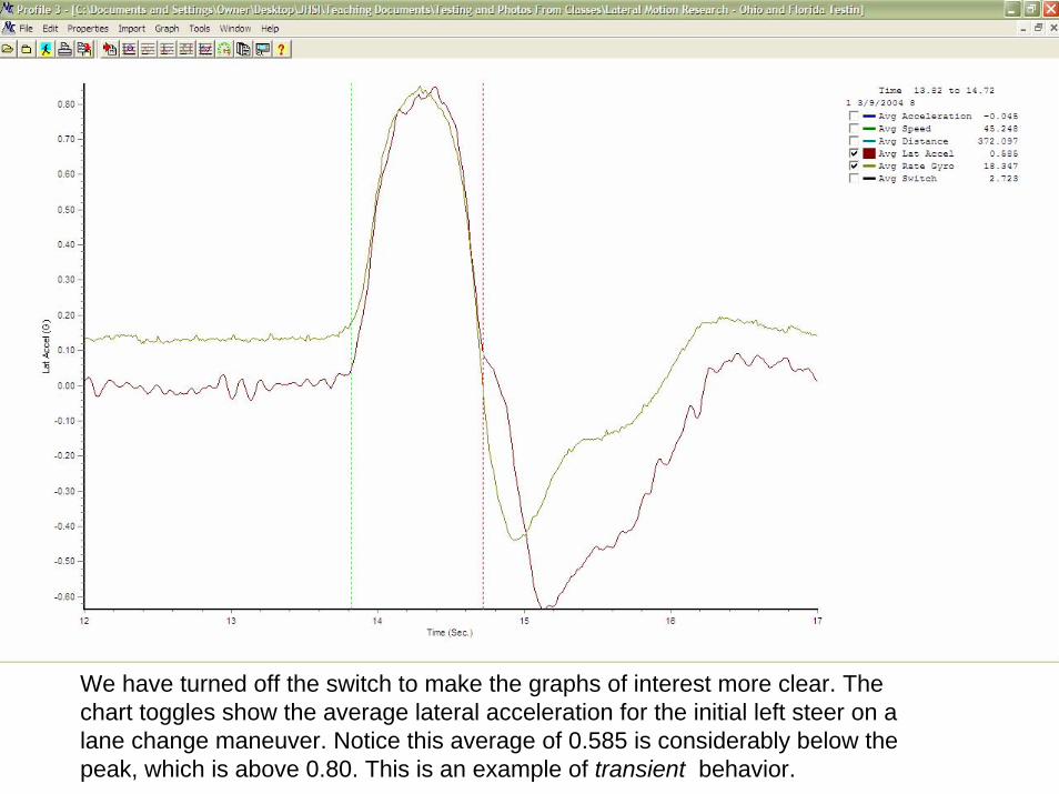
We have turned off the switch to make the graphs of interest more clear. The chart toggles show the average lateral acceleration for the initial left steer on a lane change maneuver. Notice this average of 0.585 is considerably below the peak, which is above 0.80. This is an example of transient behavior.
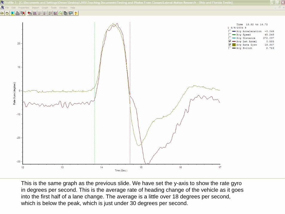
This is the same graph as the previous slide. We have set the y-axis to show the rate gyro in degrees per second. This is the average rate of heading change of the vehicle as it goes into the first half of a lane change. The average is a little over 18 degrees per second, which is below the peak, which is just under 30 degrees per second.
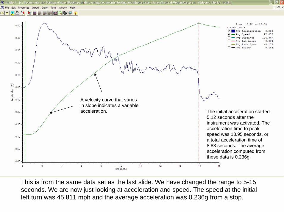
This is from the same data set as the last slide. We have changed the range to 5-15 seconds. We are now just looking at acceleration and speed. The speed at the initial left turn was 45.811 mph and the average acceleration was 0.236g from a stop.
A velocity curve that varies in slope indicates a variable acceleration. The initial acceleration started
5.12 seconds after the instrument was activated. The acceleration time to peak speed was 13.95 seconds, or a total acceleration time of 8.83 seconds. The average acceleration computed from these data is 0.236g.
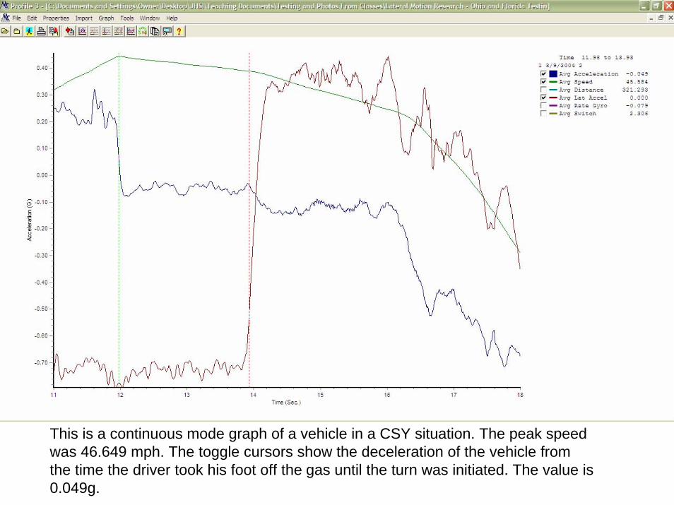
This is a continuous mode graph of a vehicle in a CSY situation. The peak speed was 46.649 mph. The toggle cursors show the deceleration of the vehicle from the time the driver took his foot off the gas until the turn was initiated. The value is 0.049g.
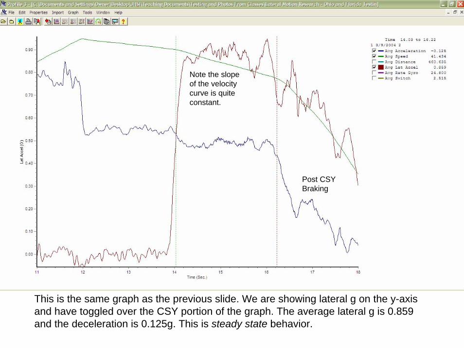
This is the same graph as the previous slide. We are showing lateral g on the y-axis and have toggled over the CSY portion of the graph. The average lateral g is 0.859 and the deceleration is 0.125g. This is steady state behavior.
Note the slope of the velocity curve is quite constant.
Post CSY Braking
Further Examples
The next several slides show the results of other testing.The accelerometer was in continuous mode, and the data extracted in the manner we have just discussed.
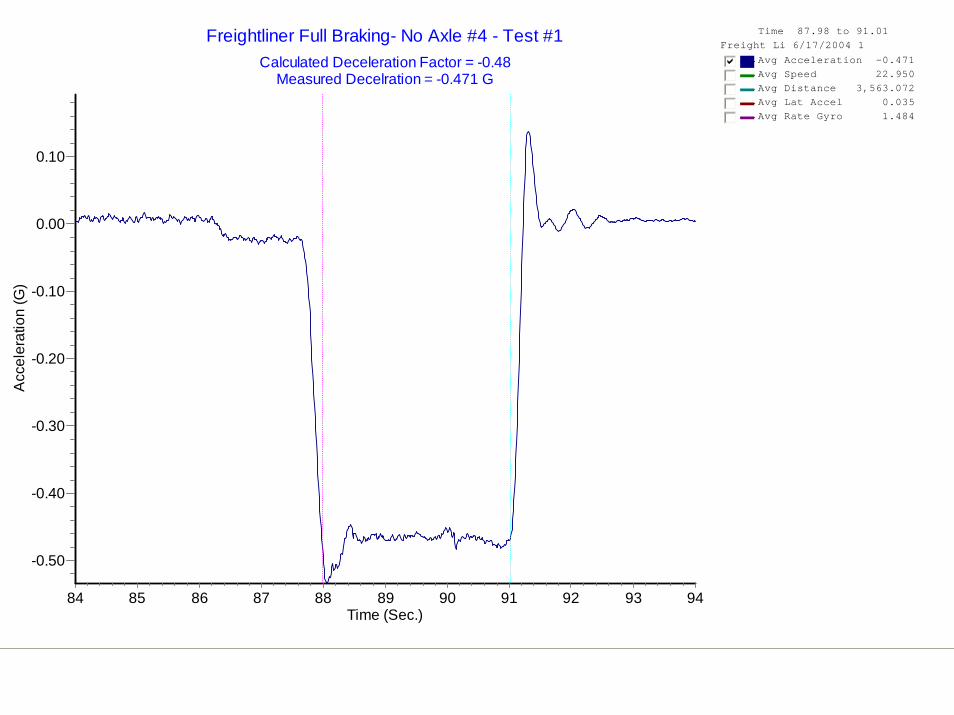
Time 87.98 to 91.01Freight Li 6/17/2004 1
Avg Acceleration -0.471gfedcbAvg Speed 22.950gfedcAvg Distance 3,563.072gfedcAvg Lat Accel 0.035gfedcAvg Rate Gyro 1.484gfedc
Freightliner Full Braking- No Axle #4 - Test #1Calculated Deceleration Factor = -0.48
Measured Decelration = -0.471 G
Time (Sec.)9493929190898887868584
Acc
eler
atio
n (G
)
0.10
0.00
-0.10
-0.20
-0.30
-0.40
-0.50
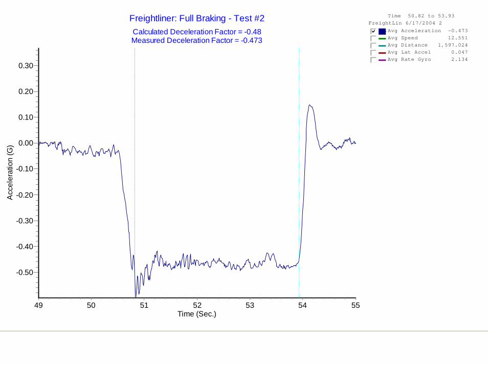
Time 50.82 to 53.93FreightLin 6/17/2004 2
Avg Acceleration -0.473gfedcbAvg Speed 12.551gfedcAvg Distance 1,597.024gfedcAvg Lat Accel 0.047gfedcAvg Rate Gyro 2.134gfedc
Freightliner: Full Braking - Test #2Calculated Deceleration Factor = -0.48Measured Deceleration Factor = -0.473
Time (Sec.)55545352515049
Acc
eler
atio
n (G
)
0.30
0.20
0.10
0.00
-0.10
-0.20
-0.30
-0.40
-0.50
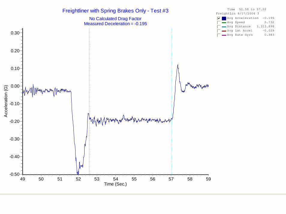
Time 52.58 to 57.02FreightLin 6/17/2004 3
Avg Acceleration -0.195gfedcbAvg Speed 5.732gfedcAvg Distance 1,313.898gfedcAvg Lat Accel -0.025gfedcAvg Rate Gyro 0.383gfedc
Freightliner with Spring Brakes Only - Test #3No Calculated Drag Factor
Measured Deceleration = -0.195
Time (Sec.)5958575655545352515049
Acc
eler
atio
n (G
)
0.30
0.20
0.10
0.00
-0.10
-0.20
-0.30
-0.40
-0.50
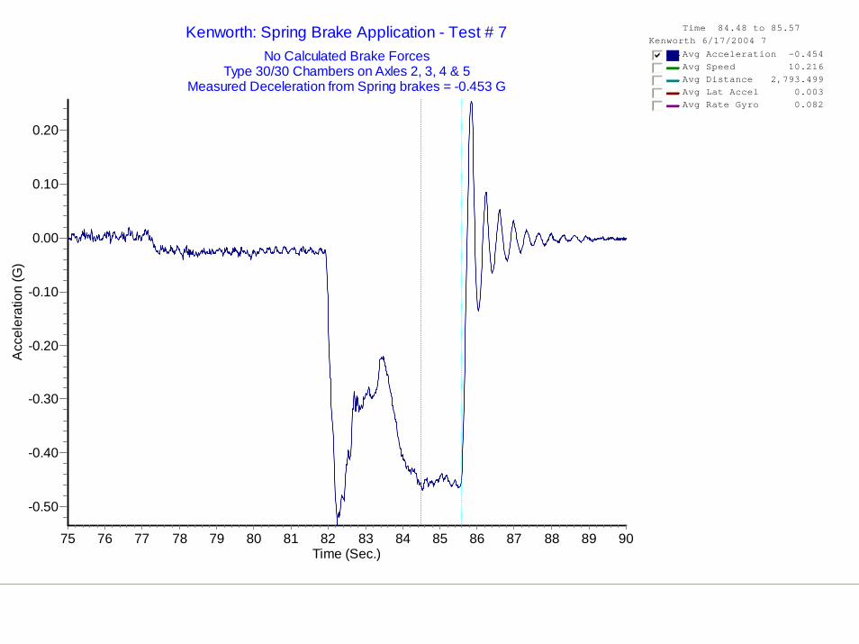
Time 84.48 to 85.57Kenworth 6/17/2004 7
Avg Acceleration -0.454gfedcbAvg Speed 10.216gfedcAvg Distance 2,793.499gfedcAvg Lat Accel 0.003gfedcAvg Rate Gyro 0.082gfedc
Kenworth: Spring Brake Application - Test # 7No Calculated Brake Forces
Type 30/30 Chambers on Axles 2, 3, 4 & 5Measured Deceleration from Spring brakes = -0.453 G
Time (Sec.)90898887868584838281807978777675
Acc
eler
atio
n (G
)
0.20
0.10
0.00
-0.10
-0.20
-0.30
-0.40
-0.50
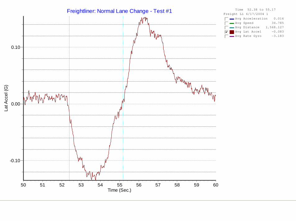
Time 52.38 to 55.17Freight Li 6/17/2004 1
Avg Acceleration 0.016gfedcAvg Speed 34.785gfedcAvg Distance 1,568.127gfedcAvg Lat Accel -0.083gfedcbAvg Rate Gyro -3.183gfedc
Freightliner: Normal Lane Change - Test #1
Time (Sec.)6059585756555453525150
Lat A
ccel
(G)
0.10
0.00
-0.10
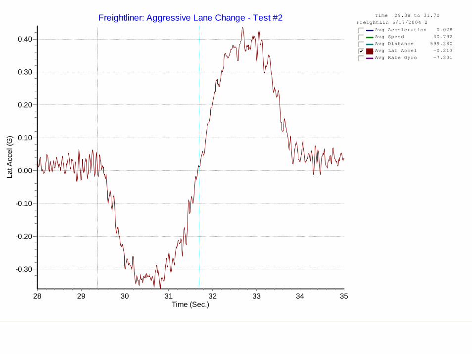
Time 29.38 to 31.70FreightLin 6/17/2004 2
Avg Acceleration 0.028gfedcAvg Speed 30.792gfedcAvg Distance 599.280gfedcAvg Lat Accel -0.213gfedcbAvg Rate Gyro -7.801gfedc
Freightliner: Aggressive Lane Change - Test #2
Time (Sec.)3534333231302928
Lat A
ccel
(G)
0.40
0.30
0.20
0.10
0.00
-0.10
-0.20
-0.30
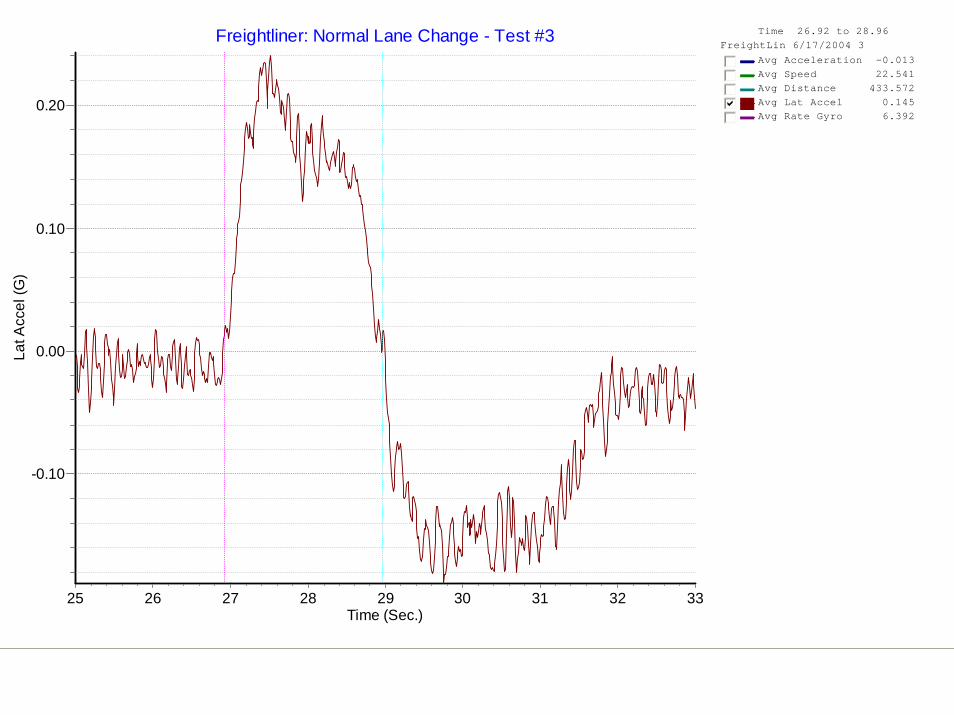
Time 26.92 to 28.96FreightLin 6/17/2004 3
Avg Acceleration -0.013gfedcAvg Speed 22.541gfedcAvg Distance 433.572gfedcAvg Lat Accel 0.145gfedcbAvg Rate Gyro 6.392gfedc
Freightliner: Normal Lane Change - Test #3
Time (Sec.)333231302928272625
Lat A
ccel
(G)
0.20
0.10
0.00
-0.10
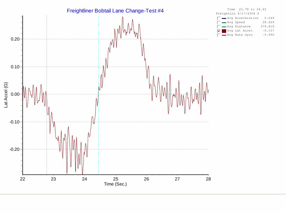
Time 22.78 to 24.45FreightLin 6/17/2004 4
Avg Acceleration 0.049gfedcAvg Speed 28.629gfedcAvg Distance 379.816gfedcAvg Lat Accel -0.157gfedcbAvg Rate Gyro -5.990gfedc
Freightliner Bobtail Lane Change-Test #4
Time (Sec.)28272625242322
Lat A
ccel
(G)
0.20
0.10
0.00
-0.10
-0.20
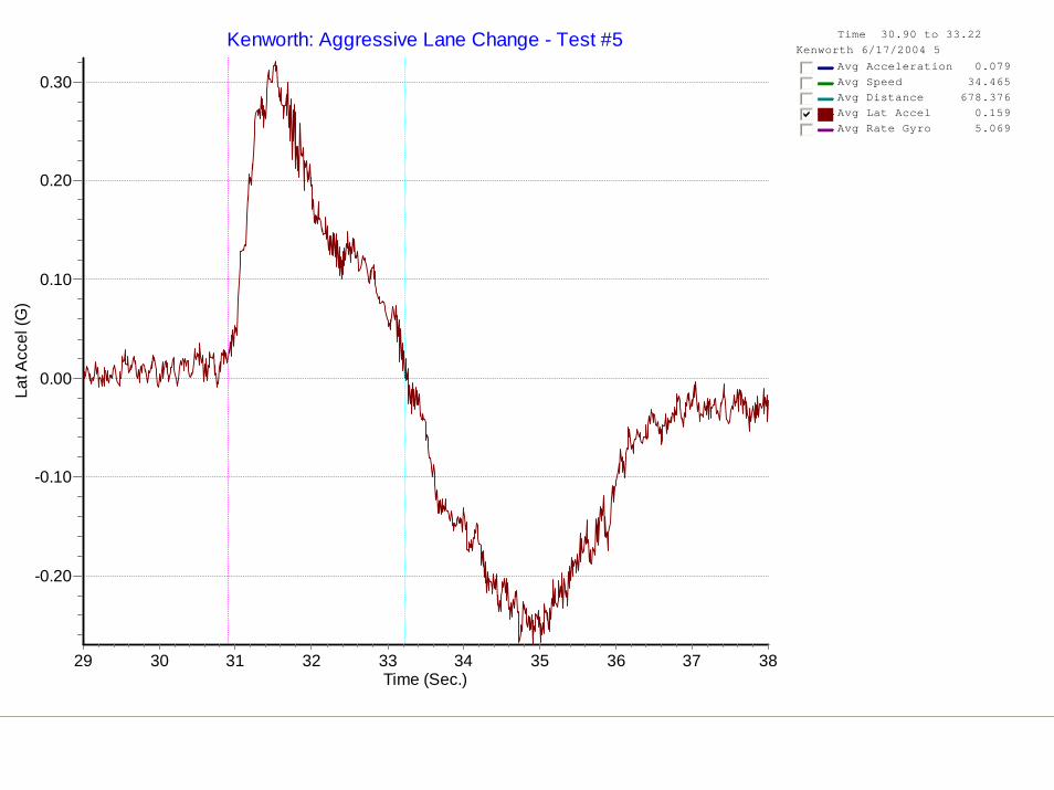
Time 30.90 to 33.22Kenworth 6/17/2004 5
Avg Acceleration 0.079gfedcAvg Speed 34.465gfedcAvg Distance 678.376gfedcAvg Lat Accel 0.159gfedcbAvg Rate Gyro 5.069gfedc
Kenworth: Aggressive Lane Change - Test #5
Time (Sec.)38373635343332313029
Lat A
ccel
(G)
0.30
0.20
0.10
0.00
-0.10
-0.20
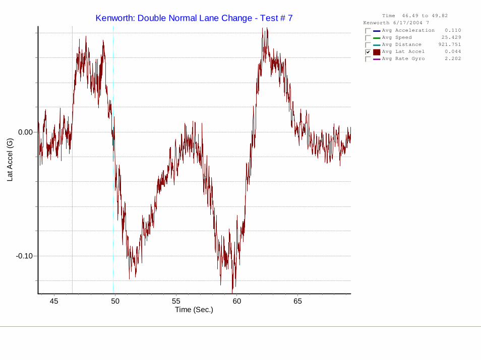
Time 46.49 to 49.82Kenworth 6/17/2004 7
Avg Acceleration 0.110gfedcAvg Speed 25.429gfedcAvg Distance 921.751gfedcAvg Lat Accel 0.044gfedcbAvg Rate Gyro 2.202gfedc
Kenworth: Double Normal Lane Change - Test # 7
Time (Sec.)6560555045
Lat A
ccel
(G)
0.00
-0.10
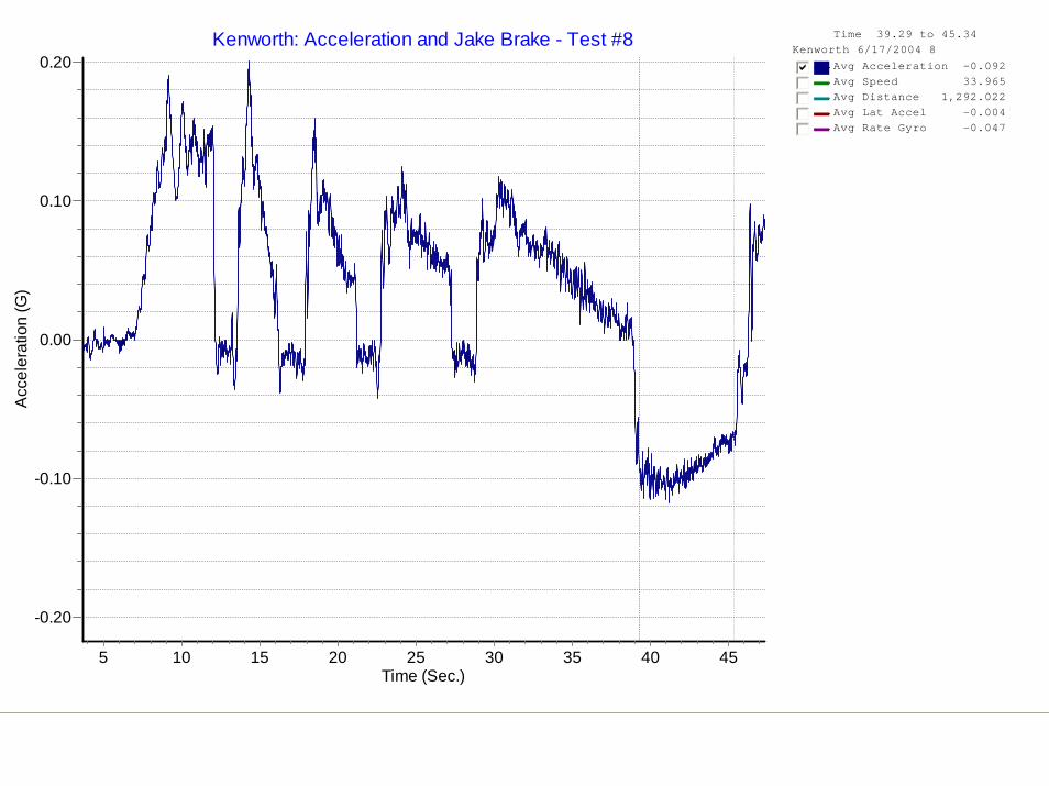
Time 39.29 to 45.34Kenworth 6/17/2004 8
Avg Acceleration -0.092gfedcbAvg Speed 33.965gfedcAvg Distance 1,292.022gfedcAvg Lat Accel -0.004gfedcAvg Rate Gyro -0.047gfedc
Kenworth: Acceleration and Jake Brake - Test #8
Time (Sec.)45403530252015105
Acc
eler
atio
n (G
)
0.20
0.10
0.00
-0.10
-0.20
Summary
In this presentation, we have examined how we may chose an accelerometer system.
The system we would use for brake testing is not the same system we would use for crash testing.
We have seen examples of how to set up and use the accelerometer to help us both measure and understand vehicle dynamics.This understanding assists us in becoming more informed and competent crash reconstructionists.