acceleration due to gravitynew2011 -...

1

Acceleration Due to Gravity

Introduction In this lab you will measure the acceleration due to gravity near the earth’s surface with two experiments: first, by determining the time for a steel ball to fall a known vertical distance (free fall), and then second, by measuring the velocity of a cart at various points as it glides down a slightly inclined and nearly frictionless track (slow fall).

Equipment Part 1: Free-Fall • Free-fall apparatus (steel plate, drop mechanism) • Electronic Timer • Steel Ball Part 2: Slow-Fall • Computer • Hard Ball, approximately 8 cm diameter • Rubber Ball, similar size • Vernier Computer Interface • Logger Pro Dynamics Cart • Vernier Motion Detector • Ruler and Meter Stick Part 1: Free Fall Acceleration Background Under the constant acceleration of gravity near the Earth’s surface, g, the vertical position, y, of a falling object is related to the time it has fallen by

!

y = y0

+ v0t "1

2gt2

where y0 and v0 are the initial position and velocity, respectively. The distance fallen after a time, t, has elapsed is:

!

y0" y =

1

2gt2" v

0t

If you release the object from rest, v0 = 0, the equation simplifies to

!

y0" y =

1

2gt2

!

By varying the distance the ball drops and measuring the corresponding transit times, we can determine the acceleration of gravity from a best fit line to a linear graph of the experimental data.

Acceleration Due to Gravity Physics 117/197/211

2

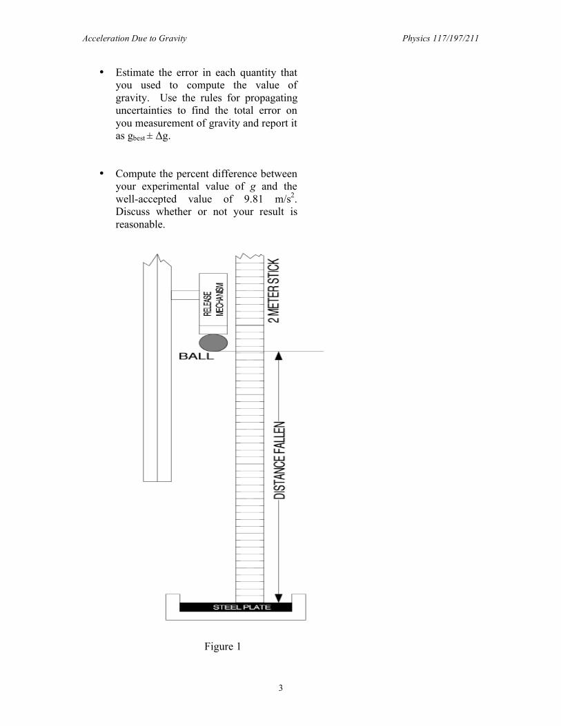
Procedure: Free-Fall Acceleration A diagram of the experimental apparatus is shown in Figure 1. When the ball loses contact with the release mechanism, the timer starts counting. It stops when the ball strikes the steel plate. The release mechanism can be adjusted vertically to vary the distance that the ball drops. Equipment Notes If you are using the Blue Timers: • Depress the POWER button until it locks in and the display comes on. • Engage the T2-T1 and TIME buttons. They should stay in, and a greenish-yellow

color should be visible through the windows on the front of the buttons. • Hold the steel ball against the indentation with a golf tee. Don’t push too hard - just

enough to click the switch. • When your hand is comfortably poised for release, first press the STOP button and

then the RESET button. The display should now read 0.00000. Everything is now ready for the release, which you should do with a swift and smooth downward motion. You may prefer to use both hands.

If you are using the Black Timers: • Turn the power switch to "ON" and the selector switch to ".0001 SEC". On some

units the selector switch is on the back. • Hold the steel ball in the indentation with a golf tee. Don’t push too hard - just

enough to click the switch. • Press the STOP button and then the RESET button; the display should read zero.

Everything is now ready for you to release the ball, which you should do with a swift and smooth downward motion. You may find it easier to use both hands.

The electronic timers can be a bit quirky in their display of leading zeros. Sometimes they will leave them out after the decimal point so that a value such as 23 milliseconds will be shown as ". 23" when it should be " .023". If you look closely you can see a blank digit where the zero should be. Furthermore, if you read it literally, the time measurements will be ten times greater than you expect, and that should tip you off.

• Measure the time of fall and the distance traveled from your starting point; record realistic uncertainties for the distance fallen and the timing measurement.

• Repeat for a total of ten distances,

ranging from near the bottom of the vertical bar to which the release mechanism is attached to as high as you can comfortably reach.

• Create a linear plot of

your data, and determine g from the slope of a best-fit line to your experimental measurements.


3

• Estimate the error in each quantity that you used to compute the value of gravity. Use the rules for propagating uncertainties to find the total error on you measurement of gravity and report it as gbest ± Δg.

• Compute the percent difference between your experimental value of g and the well-accepted value of 9.81 m/s2. Discuss whether or not your result is reasonable.

Figure 1


4

Part II: Slow Fall Acceleration

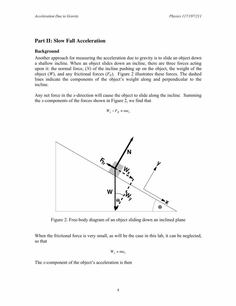
Background Another approach for measuring the acceleration due to gravity is to slide an object down a shallow incline. When an object slides down an incline, there are three forces acting upon it: the normal force, (N) of the incline pushing up on the object, the weight of the object (W), and any frictional forces (Ffr). Figure 2 illustrates these forces. The dashed lines indicate the components of the object’s weight along and perpendicular to the incline. Any net force in the x-direction will cause the object to slide along the incline. Summing the x-components of the forces shown in Figure 2, we find that

!

Wx " Ffr = max

Figure 2: Free-body diagram of an object sliding down an inclined plane

When the frictional force is very small, as will be the case in this lab, it can be neglected, so that

!

Wx

= max

The x-component of the object’s acceleration is then


5

!

ax =Wx

m=

mg sin"( )m

= g sin"

For a fixed inclination angle, θ, measurement of the acceleration down the incline permits g to be determined experimentally. Note that because the acceleration is constant we can appeal to the familiar kinematics equations to describe the motion of the object as it moves down the incline.

!

r r =

r r 0

+r v 0t +1

2

r a t2

!

r v =

r v 0

+r a t

For this lab, we are interested in ax, the acceleration of the object along the incline, so all positions, velocities, and accelerations will be associated with the x-direction. To further simplify the experiment, the initial velocity (v0) of the object will be chosen to be zero. Thus, our general equations of motion reduce to

!

x = x0

+1

2axt2

!

vx

= axt

when the +x-direction is defined to be down the incline. Experimentally, we will determine the velocity of the object after it has traveled specific distances along the incline. We can describe this mathematically by combining the previous two equations and eliminating the time variable,

!

x " x0

=1

2ax

vx( )2

The left side of the equation (x – x0) represents the distance traveled by the object. The acceleration of the object along the incline can be determined from the slope of a linear plot involving the distance the object travels and its velocity. During the early part of the seventeenth century, Galileo experimentally examined the concept of acceleration. One of his goals was to learn more about freely falling objects. Unfortunately, his timing devices were not precise enough to allow him to study free fall directly. Therefore, he decided to limit the acceleration by using fluids, inclined planes, and pendulums. In this lab exercise, you will see how the acceleration of a rolling ball or cart depends on the ramp angle. Then, you will use your data to extrapolate to the acceleration on a vertical “ramp;” that is, the acceleration of a ball in free fall. If the angle of an incline with the horizontal is small, a cart rolling down the incline moves slowly and can be easily timed. Using time and position data, it is possible to calculate the acceleration of the cart. When the angle of the incline is increased, the acceleration also increases. The acceleration is directly proportional to the sine of the incline angle, (θ). A graph of acceleration versus sin (θ ) can be extrapolated to a point where the value of sin(θ ) is 1. When sin θ is 1, the angle of the incline is 90°. This is


6

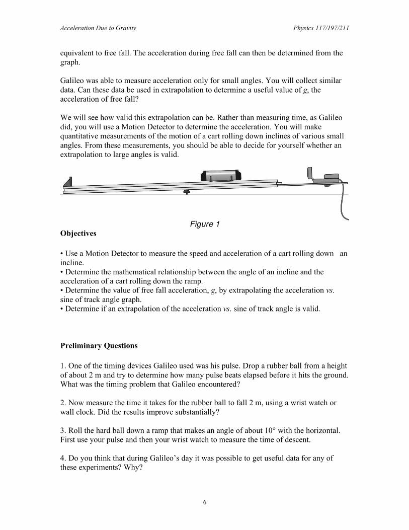
equivalent to free fall. The acceleration during free fall can then be determined from the graph. Galileo was able to measure acceleration only for small angles. You will collect similar data. Can these data be used in extrapolation to determine a useful value of g, the acceleration of free fall? We will see how valid this extrapolation can be. Rather than measuring time, as Galileo did, you will use a Motion Detector to determine the acceleration. You will make quantitative measurements of the motion of a cart rolling down inclines of various small angles. From these measurements, you should be able to decide for yourself whether an extrapolation to large angles is valid.

Figure 1

Objectives • Use a Motion Detector to measure the speed and acceleration of a cart rolling down an incline. • Determine the mathematical relationship between the angle of an incline and the acceleration of a cart rolling down the ramp. • Determine the value of free fall acceleration, g, by extrapolating the acceleration vs. sine of track angle graph. • Determine if an extrapolation of the acceleration vs. sine of track angle is valid. Preliminary Questions 1. One of the timing devices Galileo used was his pulse. Drop a rubber ball from a height of about 2 m and try to determine how many pulse beats elapsed before it hits the ground. What was the timing problem that Galileo encountered? 2. Now measure the time it takes for the rubber ball to fall 2 m, using a wrist watch or wall clock. Did the results improve substantially? 3. Roll the hard ball down a ramp that makes an angle of about 10° with the horizontal. First use your pulse and then your wrist watch to measure the time of descent. 4. Do you think that during Galileo’s day it was possible to get useful data for any of these experiments? Why?


7

Procedure 1. Connect the Motion Detector to the DIG/SONIC 1 channel of the interface. If the Motion Detector has a switch, set it to Track. 2. Elevate one end of a 1–2 m long board or track so that it forms a small angle with the horizontal. Adjust the points of contact of the two ends of the incline, so that the distance, x, in Figure 1 is between 1 and 2 m. 3. Place the Motion Detector at the top of an incline. Place it so the cart will never be closer than 0.15 m. 4. Open the file “04 g On An Incline” from the Physics with Vernier folder. 5. Hold the cart on the incline about 0.15 m from the Motion Detector. 6. Click to begin collecting data; release the cart after the Motion Detector starts to click. Get your hand out of the Motion Detector path quickly. You may have to adjust the position and aim of the Motion Detector several times before you get it right. Adjust and repeat this step until you get a good run showing approximately constant slope on the velocity vs. time graph during the rolling of the cart. 7. Logger Pro can fit a straight line to a portion of your data. First indicate which portion is to be used by dragging across the graph to indicate the starting and ending times. Then click on the Linear Fit button, to perform a linear regression of the selected data. Use this tool to determine the slope of the velocity vs. time graph, using only the portion of the data for times when the cart was freely rolling. From the fitted line, find the acceleration of the cart. Record the value in your data table. 8. Repeat Steps 5–7 two more times. 9. Measure the length of the incline, x, which is the distance between the two contact points of the ramp. See Figure 1. 10. Measure the height of the elevation , h. These last two measurements will be used to determine the angle of the incline. 11. Raise the incline. Adjust so that the distance, x, is the same as the previous reading. 12. Repeat Steps 5–10 for the new incline. 13. Repeat Steps 5–11 for different heights.


8

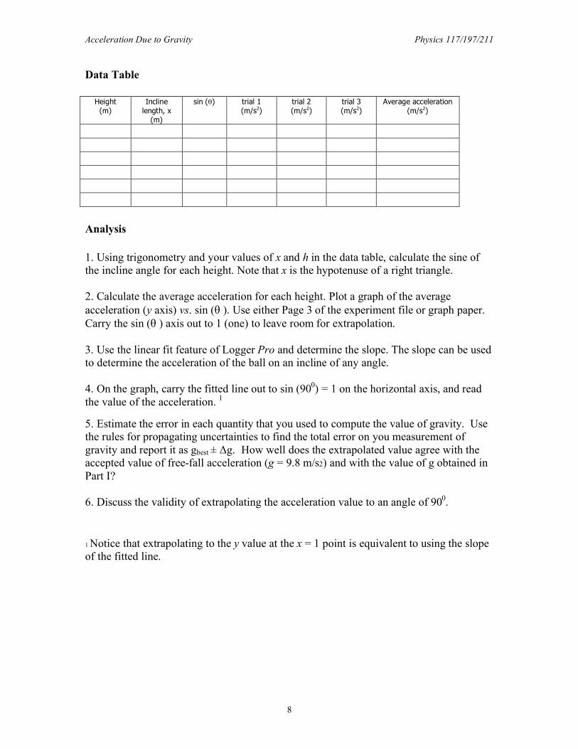
Data Table

Height (m)

Incline length, x

(m)

sin (θ) trial 1 (m/s2)

trial 2 (m/s2)

trial 3 (m/s2)

Average acceleration (m/s2)

Analysis 1. Using trigonometry and your values of x and h in the data table, calculate the sine of the incline angle for each height. Note that x is the hypotenuse of a right triangle. 2. Calculate the average acceleration for each height. Plot a graph of the average acceleration (y axis) vs. sin (θ ). Use either Page 3 of the experiment file or graph paper. Carry the sin (θ ) axis out to 1 (one) to leave room for extrapolation. 3. Use the linear fit feature of Logger Pro and determine the slope. The slope can be used to determine the acceleration of the ball on an incline of any angle. 4. On the graph, carry the fitted line out to sin (900) = 1 on the horizontal axis, and read the value of the acceleration. 1 5. Estimate the error in each quantity that you used to compute the value of gravity. Use the rules for propagating uncertainties to find the total error on you measurement of gravity and report it as gbest ± Δg. How well does the extrapolated value agree with the accepted value of free-fall acceleration (g = 9.8 m/s2) and with the value of g obtained in Part I? 6. Discuss the validity of extrapolating the acceleration value to an angle of 900. 1 Notice that extrapolating to the y value at the x = 1 point is equivalent to using the slope of the fitted line.


9

Concluding Questions When responding to the questions/exercises below, your responses need to be complete and coherent. Full credit will only be awarded for correct answers that are accompanied by an explanation and/or justification. Include enough of the question/exercise in your response that it is clear to your teaching assistant to which problem you are responding.

1. Does the acceleration of an object on an incline increase or decrease as the inclination angle gets smaller? Explain your reasoning.

2. Investigate how the value of g varies around the world. For example, how does altitude affect the value of g? What other factors cause this acceleration to vary from place to place? How much can g vary at a school in the mountains compared to a school at sea level?

!

10

=1•"

1800# 0.0175rad

acceleration due to gravitynew2011 -...

Documents