abstract manipulation of the quantum motion of …
TRANSCRIPT

ABSTRACT
Title of dissertation: MANIPULATION OF THE QUANTUMMOTION OF TRAPPED ATOMIC IONSVIA STIMULATED RAMAN TRANSITIONS
Kenneth Earl Wright IIDoctor of Philosophy, 2017
Dissertation directed by: Professor Christopher MonroeDepartment of Physics
Trapped ions have been a staple resource of quantum simulation for the past
decade. By taking advantage of the spin motion coupling provided by the Coulomb
interaction, trapped ions have been used to study quantum phase transitions of
highly frustrated spins, many body localization, as well as discrete time crystals.
However, all of these simulations involve decoupling the ion motion from spin at
the end of the experimental procedure. Here we present progress towards driving
bosonic interference between occupied phonon modes.
This thesis details a tool box for manipulating the motional states of a chain
of trapped ions. Taking advantage of spin motion interaction of tightly trapped
chains of 171Yb+ ions with two photon Raman transition, we show how to prepare
a specific number state of a given normal mode of motion. This is achieved without
traditional individual addressing but instead by using composite pulse sequences
and ion transport. This involves a stage of quantum state distillation, and we also
show preservation of phonon and spin coherence after this distillation step. This

Fock state preparation sets the stage to observe bosonic interference of different
phonon modes.
We use stimulated Raman transitions to create a parametric drive; this drive
will couple different normal modes of motion. To observe the bosonic nature of the
phonons, we preform a Hong-Ou-Mandel (HOM) interference experiment on two
singly occupied normal modes. We use the same spin motion coupling to read out
the spin states of individual ions as a witness for this interaction. We also describe
a process to use stimulated rapid adiabatic passage (STIRAP) to read out normal
mode occupation. The toolbox presented here will be useful for future experiments
towards boson sampling using trapped ions.

MANIPULATION OF THE QUANTUM MOTIONOF TRAPPED ATOMIC IONS
VIA STIMULATED RAMAN TRANSITIONS
by
Kenneth Earl Wright II
Dissertation submitted to the Faculty of the Graduate School of theUniversity of Maryland, College Park in partial fulfillment
of the requirements for the degree ofDoctor of Philosophy
2017
Advisory Committee:Professor Chris Monroe, Chair/AdvisorProfessor Gretchen CampbellProfessor Andrew ChildsProfessor Luis OrozcoProfessor James Williams

c© Copyright byKenneth Wright
2017

Dedication
to
Monica Gutierrez Galan,
Sally Morris, James Morris, and Kenneth Wright Sr
ii

Table of Contents
Dedication iv
Acknowledgments iv
List of Figures v
1 Introduction 1
2 Ion Trapping 52.1 Paul Traps . . . . . . . . . . . . . . . . . . . . . . . . . . . . . . . . . 5
2.1.1 Ion trap theory . . . . . . . . . . . . . . . . . . . . . . . . . . 62.1.2 Macro-fabricated traps . . . . . . . . . . . . . . . . . . . . . . 102.1.3 Micro-fabricated traps . . . . . . . . . . . . . . . . . . . . . . 12
2.2 Normal Modes . . . . . . . . . . . . . . . . . . . . . . . . . . . . . . . 162.3 Yb Ions . . . . . . . . . . . . . . . . . . . . . . . . . . . . . . . . . . 19
2.3.1 Ionization . . . . . . . . . . . . . . . . . . . . . . . . . . . . . 202.3.2 Doppler Cooling . . . . . . . . . . . . . . . . . . . . . . . . . . 222.3.3 Spin Sate Initialization and Readout . . . . . . . . . . . . . . 26
3 Experimental Apparatus 293.1 Vacuum Chamber . . . . . . . . . . . . . . . . . . . . . . . . . . . . . 29
3.1.1 External Chamber Components . . . . . . . . . . . . . . . . . 303.1.2 Internal Chamber Components . . . . . . . . . . . . . . . . . 32
3.2 Optics . . . . . . . . . . . . . . . . . . . . . . . . . . . . . . . . . . . 353.2.1 Cooling and Trapping Beam Paths . . . . . . . . . . . . . . . 353.2.2 Imaging system . . . . . . . . . . . . . . . . . . . . . . . . . . 423.2.3 Raman Beam Path . . . . . . . . . . . . . . . . . . . . . . . . 45
3.3 Control Electronics . . . . . . . . . . . . . . . . . . . . . . . . . . . . 493.3.1 Timing Control . . . . . . . . . . . . . . . . . . . . . . . . . . 493.3.2 Trapping Voltage Control . . . . . . . . . . . . . . . . . . . . 51
3.3.2.1 DC Voltages . . . . . . . . . . . . . . . . . . . . . . 523.3.2.2 RF Voltage . . . . . . . . . . . . . . . . . . . . . . . 54
3.3.3 Stabilization . . . . . . . . . . . . . . . . . . . . . . . . . . . . 56
iii

3.4 Ball Grid Array Trap . . . . . . . . . . . . . . . . . . . . . . . . . . . 58
4 Coherent Operations 624.1 Raman Interaction . . . . . . . . . . . . . . . . . . . . . . . . . . . . 62
4.1.1 Pulsed Raman Interaction . . . . . . . . . . . . . . . . . . . . 714.1.2 Yb Ion Coupling . . . . . . . . . . . . . . . . . . . . . . . . . 724.1.3 Raman Coupling with Normal Modes . . . . . . . . . . . . . . 764.1.4 STIRAP . . . . . . . . . . . . . . . . . . . . . . . . . . . . . . 82
5 Phonon Toolbox 865.1 Sideband Cooling . . . . . . . . . . . . . . . . . . . . . . . . . . . . . 87
5.1.1 Heating Rates . . . . . . . . . . . . . . . . . . . . . . . . . . . 895.2 Individual Addressing . . . . . . . . . . . . . . . . . . . . . . . . . . . 91
5.2.1 Transport . . . . . . . . . . . . . . . . . . . . . . . . . . . . . 925.2.2 Composite pulse sequences . . . . . . . . . . . . . . . . . . . . 94
5.3 Phonon State Initialization and Distillation . . . . . . . . . . . . . . . 1005.4 Readout . . . . . . . . . . . . . . . . . . . . . . . . . . . . . . . . . . 108
6 Phonon Interference 1116.1 Hong-Ou-Mandel Photon Example . . . . . . . . . . . . . . . . . . . 1116.2 Hong-Ou-Mandel Phonon Example . . . . . . . . . . . . . . . . . . . 118
6.2.1 Results . . . . . . . . . . . . . . . . . . . . . . . . . . . . . . . 122
7 Outlook 1307.1 Future Improvements . . . . . . . . . . . . . . . . . . . . . . . . . . . 130
A Laser locking 133A.1 Wavemeter Locking . . . . . . . . . . . . . . . . . . . . . . . . . . . . 133A.2 Locking via discharge cells . . . . . . . . . . . . . . . . . . . . . . . . 135A.3 Transfer Cavity Locking . . . . . . . . . . . . . . . . . . . . . . . . . 138
B Boson Sampling 141
Bibliography 144
iv

List of Figures
2.1 Florescence image of eight ion image . . . . . . . . . . . . . . . . . . 62.2 Linear Paul trap . . . . . . . . . . . . . . . . . . . . . . . . . . . . . 72.3 Linear Paul trap quadrapole . . . . . . . . . . . . . . . . . . . . . . . 82.4 Planar trap . . . . . . . . . . . . . . . . . . . . . . . . . . . . . . . . 122.5 Surface trap pseudopotential . . . . . . . . . . . . . . . . . . . . . . . 132.6 Surface trap confinement in three dimensions . . . . . . . . . . . . . . 142.7 Equally spaced four ion image . . . . . . . . . . . . . . . . . . . . . . 152.8 Three ion normal modes . . . . . . . . . . . . . . . . . . . . . . . . . 192.9 Energy levels 171Yb+ . . . . . . . . . . . . . . . . . . . . . . . . . . . 212.10 Energy levels for neutral Yb . . . . . . . . . . . . . . . . . . . . . . . 222.11 Doppler cooling scheme . . . . . . . . . . . . . . . . . . . . . . . . . . 232.12 Detection scheme . . . . . . . . . . . . . . . . . . . . . . . . . . . . . 262.13 Optical pumping scheme . . . . . . . . . . . . . . . . . . . . . . . . . 272.14 Optical pumping time scan . . . . . . . . . . . . . . . . . . . . . . . . 28
3.1 Vacuum chamber . . . . . . . . . . . . . . . . . . . . . . . . . . . . . 313.2 Oven assembly . . . . . . . . . . . . . . . . . . . . . . . . . . . . . . 343.3 399 nm optics layout . . . . . . . . . . . . . . . . . . . . . . . . . . . 363.4 935 nm optics layout . . . . . . . . . . . . . . . . . . . . . . . . . . . 373.5 369 nm optics layout . . . . . . . . . . . . . . . . . . . . . . . . . . . 383.6 Doppler cooling scheme, re-print . . . . . . . . . . . . . . . . . . . . . 393.7 S1/2 → P1/2 resonance curve . . . . . . . . . . . . . . . . . . . . . . . 403.8 Optical pumping scheme, re-print . . . . . . . . . . . . . . . . . . . . 413.9 Atomic energy levels used for detecting the spin state of the ion . . . 423.10 Histograms of bright and dark ions . . . . . . . . . . . . . . . . . . . 433.11 Optical layout of the ion imaging system . . . . . . . . . . . . . . . . 433.12 Spot diagrams for ions at the image place . . . . . . . . . . . . . . . 443.13 355 nm optics layout . . . . . . . . . . . . . . . . . . . . . . . . . . . 463.14 Chamber optics layout . . . . . . . . . . . . . . . . . . . . . . . . . . 473.15 Raman laser layout at the trap . . . . . . . . . . . . . . . . . . . . . 483.16 Control architecture . . . . . . . . . . . . . . . . . . . . . . . . . . . 493.17 Butterworth filter schematic . . . . . . . . . . . . . . . . . . . . . . . 52
v

3.18 Butterworth filter transfer function . . . . . . . . . . . . . . . . . . . 533.19 Helical resonator cross section . . . . . . . . . . . . . . . . . . . . . . 553.20 Resonator lumped element model . . . . . . . . . . . . . . . . . . . . 563.21 Repetition rate lock . . . . . . . . . . . . . . . . . . . . . . . . . . . . 583.22 BGA trap schematic . . . . . . . . . . . . . . . . . . . . . . . . . . . 593.23 Spherical octagon . . . . . . . . . . . . . . . . . . . . . . . . . . . . . 60
4.1 Clebsch Gordon . . . . . . . . . . . . . . . . . . . . . . . . . . . . . . 744.2 Carrier rabi flopping . . . . . . . . . . . . . . . . . . . . . . . . . . . 774.3 STIRAP theory . . . . . . . . . . . . . . . . . . . . . . . . . . . . . . 84
5.1 Sideband asymmetry, all three modes . . . . . . . . . . . . . . . . . . 885.2 Heating rate on mode b0 . . . . . . . . . . . . . . . . . . . . . . . . . 905.3 Sideband asymmetry after transport . . . . . . . . . . . . . . . . . . 935.4 Population transfer for composite pulse sequences . . . . . . . . . . . 945.5 Spin dynamics in a field gradient with composite pulse sequences . . 955.6 Spin dynamics with a single pulse . . . . . . . . . . . . . . . . . . . . 965.7 Single pulse . . . . . . . . . . . . . . . . . . . . . . . . . . . . . . . . 975.8 SK1 pulse . . . . . . . . . . . . . . . . . . . . . . . . . . . . . . . . . 975.9 Spin dynamics with an SK1 pulse sequence . . . . . . . . . . . . . . . 985.10 N2 pulse . . . . . . . . . . . . . . . . . . . . . . . . . . . . . . . . . . 985.11 Spin dynamics with an N2 pulse sequence . . . . . . . . . . . . . . . 995.12 Phonon preparation theory . . . . . . . . . . . . . . . . . . . . . . . . 1005.13 Phonon preparation experiment . . . . . . . . . . . . . . . . . . . . . 1025.14 Red sideband on mode b0 theory after preparation . . . . . . . . . . . 1035.15 Red sideband on mode b0 after preparation . . . . . . . . . . . . . . . 1055.16 Red sideband on mode b2 theory after preparation . . . . . . . . . . . 1065.17 Red sideband on mode b2 after preparation . . . . . . . . . . . . . . . 1075.18 STIRAP readout scheme . . . . . . . . . . . . . . . . . . . . . . . . . 109
6.1 Optical Hong-Ou-Mandel experiment . . . . . . . . . . . . . . . . . . 1126.2 Phonon HOM theoretical spin dynamics . . . . . . . . . . . . . . . . 1226.3 Phonon HOM theoretical phonon dynamics . . . . . . . . . . . . . . . 1236.4 Experimental HOM results . . . . . . . . . . . . . . . . . . . . . . . . 1256.5 Blue sideband OVAD . . . . . . . . . . . . . . . . . . . . . . . . . . . 1276.6 Blue sideband OVAD after improvements . . . . . . . . . . . . . . . . 128
A.1 Discharge cell optics layout . . . . . . . . . . . . . . . . . . . . . . . . 135A.2 Transfer cavity optics layout . . . . . . . . . . . . . . . . . . . . . . . 138
vi

Chapter 1: Introduction
The last century of physics has been one of great advancement in the under-
standing of macroscopic and microscopic processes. The advent of quantum the-
ory has lead to a deep understanding of physical systems that range in scale from
the inner workings of atoms to the inner workings of suns; modern society is full
of advancements created through better understanding of the effects of quantum
mechanics. For this alone, the importance of current quantum theory cannot be
overstated.
However, to study highly complicated many body quantum dynamics that
underlay important and practical applications of quantum mechanics, adequate tools
still remain elusive [1]. For example the natural catalysis that chemically fixes
nitrogen, is accomplished by simple bacteria and is one that, as a society, we spend
a vast amount of energy resources replicating. This process in integral to creating
the fertilizers necessary to grow food for the ever increasing world population. A
better understanding of this process might lead to a much more efficient way to feed
ourselves. This specific example is one of many that highlight the necessity for a
better understanding and implementation of tools that can be used to understand
complex quantum systems.
1

The idea of using a well understood, controlled quantum system to study a
more complicated intractable quantum system goes back to Feynman [2]. To store
the full quantum mechanical description for a large many body state classically
would require a system to store 2N complex amplitudes; where a quantum system
would only need N well controlled quantum resources. In response to this idea,
a vast field of physics has developed to try and create and manipulate quantum
resources.
Trapped atomic ions have for some time been a workhorse of experimental
quantum information science and quantum simulation. The reason that atomic
resources are so attractive for these applications is that all ions are in principle
created equal, therefore ions make for very clean quantum systems which can be
used as the basis for quantum computation or quantum simulation. The resources
almost exclusively used in trapped ion quantum systems are the internal degrees of
freedom of the ion’s electronic structure. However, this is not the only quantum
resource available to us when trapping ions. The external degrees of freedom, if
they can be cleanly initialized and manipulated, represent an interesting resource for
quantum simulation and remain widely unstudied in the community of ion trappers.
In this thesis, I will outline a set of tools we have developed with our trapped
ion system to better manipulate and initialize these external degrees of freedom.
This is done with an eye towards performing a proof of principle demonstration of
bosonic interference using the phonon excitations associated with a chain of trapped
ions. The thesis is broken out in seven chapters,
2

• Chapter 2: The basic theory of RF Paul traps; differences between macro-
fabricated and micro-fabricated traps. The normal modes of motion of a
trapped ion chain. It will also cover the incoherent atom-light interactions
which govern ionization, spin state preparation, spin readout, and Doppler
cooling.
• Chapter 3: Experimental apparatus including the vacuum system, the layout
of all of the optics from lasers to ions, as well as the optics used to image
ion florescence. The control loops that are used to lock various frequencies
and amplitudes throughout the lab are discussed, as well as a description of
the control electronics used to implement experimental sequences and collect
information about ion states.
• Chapter 4: Atom light interactions which we implement to drive coherent
operations. Including a toy description of Raman coupling via an excited state,
generalization of this model to 171Yb+ and mutli-ion chains. A description of
an adiabatic passage via the same laser fields is also discussed.
• Chapter 5: Description of the experimental procedure that we implement to
initialize and readout phonons, including data on our ability to prepare Fock
states of motion through composite pulse sequences and shuttling, as well as
our ability to distill these states through measurement.
• Chapter 6 : An example of photon interference and the observed Hong-Ou-
Mandel dip is discussed. Drawing an analogy with photonic experiments I de-
3

scribe how we intend to drive beam splitter-like interactions with the phonons
of our trapped ion chain.
• Chapter 7: Highlights some of the planned improvements, explaining how I
think these renovations of the experiment will help us reach our experimental
goals.
4

Chapter 2: Ion Trapping
2.1 Paul Traps
For the last two decades or more, ions have been used as cutting edge tools in
the development of quantum information processors as well as quantum simulators
[3–9]. One reason why ions are such a useful tool is that once confined, the atoms
are generally confined for substantial periods of time, this can be as much as several
days. This allows for repeated interrogation of the same ions. Another reason is that
each ion is identical, and unlike many other quantum systems being considered as
candidate qubits or quantum simulators, such as quantum dots or supper conducting
qubits, there is very little calibration of the qubit states themselves between different
experimental implementations1.
There are two ways in which researchers trap atomic ions, Penning traps and
Paul traps [10,11]. Penning traps rely on the cyclotron motion of charged particles
in a strong magnetic field to confine ions radially. Alternatively, Paul traps makes
use of only electric fields to confine atoms. All the work described in this thesis will
make use of Paul traps, specifically micro-fabricated linear Paul traps. I will spend
1The hyperfine splitting between the 171Yb+ clock states is the same for every laboratorytrapping Yb.
5

Figure 2.1: Eight ions trapped in the apparatus discussed in this thesis, the darkspaces are from ions which have been pumped to long lived dark states. These statesare efficiently re-pumped with the Raman laser we employ and in general are notan issue for our experiments. This chain was constructed in a deterministic fashionmoving ions between zones in a micro-fabricated trap.
the next sections on the theory background of the Paul trap, then elaborate on the
distinctions between macro-fabricated and micro-fabricated traps.
2.1.1 Ion trap theory
One might naively assume that by appropriately shaping direct current (DC)
potentials one would be able to create a potential minima in space that a charged
ion would find confining. Unfortunately, this of course violates Earnshaw’s theorem.
∇ ·E = 0 (2.1)
Which is to say that static electric fields will only have maxima or minima at
locations of charge density and that in free space there can be no local maxima or
minima of the field. The way ion trappers get around this is by applying oscillating
electric fields. Instantaneously, these fields do not violate Earnshaw’s theorem, but
if the frequency of oscillation can be made large enough, such that an ion experiences
a time average minima of the field, it will be trapped.
6

Figure 2.2: The copper colored rods here carry the RF potential, the brass coloredrods act as grounds for the RF voltage and the needles in blue, which act as “end-caps”, supply a large DC field in the axial direction of the trap. With these electrodesone can achieve three dimensional confinement.
The way this is accomplished is by creating a saddle point potential between
four electrodes which have spatial extent along an axial direction, z. Two of these
electrodes carry radio frequency power (RF) and are diagonal from each other, the
other two electrodes are grounded. This sets up an oscillating qudrapole field at
the center of these electrodes along the axis z of the trap. The radial escape route
of an ion sitting in the center of this quadrupole is rotating as the RF electrodes
oscillate between positive and negative cycles. An ion experiences a radial saddle
point potential of the form [3],
Φx,y =VRF
2cos(ΩRF t)
(1 +
x2 − y2
R2
)(2.2)
Where R is the characteristic distance of the trap, for RF traps this is the
7

Figure 2.3: By applying oscillating RF fields between diagonal rods with groundedrods adjacent to these rods sets up an oscillating quadrapole at a point equi-distantfrom all the rods along z. If this quadrapole oscillates fast enough trapped chargeswill see harmonic confinement radially from this point.
distance to the RF rail, VRF and ΩRF are the voltage and driving frequency of the
RF. To confine ions along the z axis, so called “end-cap” electrodes are placed at
the ends of the four electrodes forming the quadrapole field. By applying voltages
to these electrodes one can create harmonic confinement along the axial direction
of the trap. The potential takes the form,
Φz = U0
(z2 − x2 + y2
2
)(2.3)
We can verify that by looking at the total potential Earnshaw’s theorem is
still satisfied. The total potential is give by,
Φtotal =VRF
2cos(ΩRF t)
(1 +
x2 − y2
R2
)+ U0
(z2 − x2 + y2
2
)(2.4)
This gives an electric field with the following form which we can evaluate to
verify that Earnshaw’s theorem is still satisfied with the total potential,
8

E = −∇Φtotal (2.5)
= VRF cos(ΩRF t)
(yy − xxR2
)+ 2U0
(xx+ yy
2− zz
)(2.6)
∇ ·E =
(VRF
2− VRF
2
)cos(ΩRF t) + 2
(U0 + U0
2− U0
)(2.7)
= 0 (2.8)
From this equation for the electric field we can determine the force, F = qE,
and the equations of motion, ri − Fim
= 0,
x+
[eVRFmR2
cos(ΩRF t) +−eU0
m
]x = 0 (2.9)
y +
[−eVRFmR2
cos(ΩRF t) +−eU0
m
]y = 0 (2.10)
z +
[2eU0
m
]z = 0 (2.11)
Notice that all of these equations can be cast in the form of a Mathieu equa-
tions, ri + Ω2
4[ai + 2qi cos(ωt)] ri = 0, where the values of the unitless parameters ai
and qi define regions of trap stability. We can solve the Mathieu equations, and for
our purposes by keeping ai and qi 1, we can achieve a stable trap. The radial
solutions to the Mathieu equations take the following for.
9

ri = Ai cos(ωit+ φi)
[1 +
qi2
cos(ΩRF t) +q2i
32cos(2ΩRF t)
](2.12)
+ Aiβiqi2
sin(ωit+ φi) sin(ΩRF t) (2.13)
Where Ai depends on initial conditions and βi ≈ (ai+q2i
2)1/2, βi can be related
to the secular frequencies ωi by the relation ωi = βiΩRF
2. By defining these unitless
parameters in terms of the above trap parameters, we can also relate them to the
secular frequencies of the trap.
ax =−4eU0
mΩ2RF
qx =2eVRFmR2Ω2
RF
ωx =eVRF√
2mR2ΩRF
(2.14)
ay =−4eU0
mΩ2RF
qy =−2eVRFmR2Ω2
RF
ωy =eVRF√
2mR2ΩRF
(2.15)
az =8eU0
mΩ2RF
qz = 0 ωz =
√2eU0
m(2.16)
By controlling these parameters, we can affect the ion spacing and frequen-
cies of the normal modes of motion. It is important to directly fix some of these
parameters because of the direct impact on mode frequency. The next subsections
will discuss some of the differences between macro- and micro-fabricated ion traps.
2.1.2 Macro-fabricated traps
The more traditional traps which are still the main workhorses of most ion
trapping laboratories are what are known as macro-traps. In the ion trapping labo-
10

ratories at the University of Maryland we, almost exclusively, use blade traps [12–14];
where the four rods of the canonical Paul trap are formed by four thin segmented
blades. Two of these blades carry RF voltage to the trap, the other two have DC
potentials applied to their segments. These electrodes act as “end-caps” and this
segmentation allows for some shuttling of ions. Although, these procedures are quite
limited due to the small amount of segmentation. When they have segmented DC
electrodes, macro-traps tend to have only a few trapping zones. These traps usually
have dimensions on the scale of inches and are generally constructed by hand in a
laboratory setting. The ion to trap electrode distance can be quite small, on the
order of 100 µm. The greatest benefit of traps like this is that they have extremely
large well depths. The typical macro-trap can have well depths of approximately 10
eV, which corresponds to a temperature of 1 · 105 K, these traps have been known
to hold ions for weeks at a time.
The primary disadvantage of traps like this is that they are not scalable. If
one really wanted to build a large scale quantum information processor, they would
need thousands of ions or ion chains in separate traps coupled together [15, 16].
Holding progressively longer chains of ions in a single trap will eventually be limited
by vacuum and is therefore inherently unscalable. Coupling separate traps together
has promise, however if all of these traps need to be built by hand, where each trap
will be different and those differences need to be calibrated away, this also seems
like a no-go situation. That begin said, all of the most cutting edge work on high
fidelity gates [17], quantum simulation [18], or large entangled states [7] are still
performed on these traps.
11

2.1.3 Micro-fabricated traps
Figure 2.4: By laying out the rods of the traditional Paul trap one can make a trapwhere all electrodes are in one plane and the oscillating quadrapole potential liesabove the plane.
In contrast to the macro-fabricated traps of the previous section, micro-fabricated
traps were designed with the idea of scalability specifically in mind. For our pur-
poses, a micro-fabricated trap will be any trap which was produced in a CMOS
like foundry. In particular, this experiment has only used traps which consist of
etched metal features on silicon resulting in a planar geometry2. The general four
wire geometry we described earlier in this chapter for larger ion traps still applies to
micro-fabricated traps, however the geometry of electrodes is clearly modified. Con-
sider the same four rods as before but instead lay them out in a single plane, insert
2That is not to say that more symmetric three dimensional geometries are not considered micro-fabricated [19], only that they differ so slightly from the macro-fabricated traps that the theory ofoperation is essentially the same [20].
12

Figure 2.5: Simulation of the pseudo-potential above the micro-fabricated trap wecurrently are using, the color scale is in meV This null is found approximately 60µm above the trap surface and is 60 meV deep. The orientation of the cross hairsindicates the direction of the RF principal axes.
a DC electrode between the two RF electrodes, and assume that at infinity above
the surface there is a grounded plane. There will be a quadrapole potential, just as
before, above this plane [21]. If we flatten out these electrodes we have a standard
planar ion trap. The pseudo-potential tube is now located above the surface and
extends along the electrodes. Any or all of the DC electrodes can be segmented to
apply harmonic confinement along the axis.
The obvious advantage of traps formed in this way is that it allows for very
small structures to be built into the trapping architecture. The electrodes them-
selves can take on rather exotic shapes, and although this must be taken into account
when modeling the trap, there have been quite a range of novel architectures fabri-
13

Figure 2.6: Simulations of our trapping structure showing the transverse confine-ment as a function of the axial position along the trap, color scale in meV. Byshifting voltages on the DC electrodes this potential can be moved anywhere alongthe z axis.
cated into micro-fabricated ion traps. This includes slots to have laser beams pass
through the trapping structure [22], mirrors both concave [23,24] and diffractive [25],
junctions to send ions along different arms of crossed linear traps [26,27], as well as
microwave wave guides to couple atoms to near-field microwaves [28]. The discus-
sion of the particular trap used for these experiments is left to the next chapter. In
particular, having many electrodes which are small in extent allows for fine control
of the DC potential. This gives us the flexibility to adjust ion spacing as well as
modify the harmonicity of the DC potential. This allows us to make ions equally
spaced, or spaced widely apart to help in imaging individual ions. In general this
is more difficult for macro-fabricated traps where there are a limited number of
electrodes and they are far away, this in particular makes creating anharmonic DC
potentials more challenging.
14

Figure 2.7: Florescence image of four equally spaced ions, achieved by adjusting theproportion of harmonic and anharmonic terms in the axial potential. The four ionsare mostly imaged onto 4 circular spots onto the camera, however the residual lightaround these spots highlights imperfections in the imaging system.
The biggest problem for micro-fabricated traps also is that the trapping struc-
tures are so small, which limits the transverse confinement and the well depth that
can be achieved, and increases the heating rate. Because the structures that form
the RF electrodes are separated from adjacent ground planes by approximately 4
µm, at high enough voltage the RF will arc to ground. This process is violent and
can destroy the RF electrode. This puts a hard limit on the maximum amplitude
of the RF voltage that can be applied, which is directly proportional to transverse
trap frequency.
The RF potential of micro-fabricated traps is generally not as symmetric as
macro-fabricated traps, because of this it is harder to have a strong quadrapole
field. The strength of the field can be thought of as the depth of the radial con-
finement. Generally these traps have well depths of < 100 meV, for comparison
that corresponds to a temperature of 103 K. This means that ions routinely can be
boiled out of the trap due to collisions or general heating. The lifetime of chains in
micro-fabricated traps rarely exceeds days as opposed to weeks in the their macro-
fabricated counterparts.
The heating of ions is made especially worse in micro-traps because of the so
15

called “anomalous heating rate”, which has been found to scale approximately as
1/R4 [29], where R is the distance away from the nearest trapping surface3. With
electrodes so close to the ions this problem has limited the acceptance of micro-
fabricated traps in the community up until fairly recently.
2.2 Normal Modes
The external quantum degrees of freedom we are trying to initialize and ma-
nipulate are the excitations of the normal modes of motion of the ions. In the
low excitation limit, we can think of these excitations as bosonic particles known
as phonons. This thesis will describe the progress we have made in controlling
the number states of these phonons. It is therefore necessary to discuss how these
normal modes of motion arise in our physical system. In the previous section we
derived harmonic confinement in all three dimensions resulting from voltages ap-
plied to electrodes. To determine the collective modes of motion of the ion chain we
should balance this restoring potential with the Coulomb repulsion between ions.
Let us consider the full Hamiltonian for an arbitrary number of ions [30]
H = K + V (2.17)
=N∑i
3∑j
p2i,j
2m+
1
2mω2
i,jq2i,j +
∑i,k
e2
4πε0
1
di,k(2.18)
3 To be clear this distance can be quite similar to macro-fabricated traps, however the welldepth is so much lower that this heating rate can adversely effect ion lifetimes.
16

Where qi,j is the canonical position not the equilibrium position. The sum
over j is a sum over the different trapping directions, i and k are sums over the ions,
and di,k is the distance between ions i and k. We will assume here that ωx,y ωz;
this ensures that ion equilibrium positions will lie in a line along the z axis of the
trap. We need to calculate[∂V∂qz,i
]q0z,i
= 0 to determine the equilibrium positions of
the ions along this line.
0 = mω2zzi −
i−1∑k=1
e2
4πε0
1
|zi − zk|2+
N∑k=i+1
e2
4πε0
1
|zi − zk|2(2.19)
= zi +e2
4πε0mω2z
(N∑
k=i+1
1
|zi − zk|2−
i−1∑k=1
1
|zi − zk|2
)(2.20)
= uid0 +e2
4πε0mω2z
1
d20
(N∑
k=i+1
1
|ui − uk|2−
i−1∑k=1
1
|ui − uk|2
)(2.21)
= ui +N∑
k=i+1
1
|ui − uk|2−
i−1∑k=1
1
|ui − uk|2(2.22)
This equation can be numerically evaluated for any number of ions to de-
termine their equilibrium positions along the axial trapping direction. We de-
fine the unitless length ui = zid0
with the characteristic distance between ions,
d0 =(
e2
4πε0mω2z
) 13. If we expand the potential to second order in a Taylor expansion
about these equilibrium positions, in any direction, we can calculate the normal
17

modes of motion in that direction. More formally, we write the Lagrangian,
L = K − U (2.23)
=N∑i
1
2m ˙q2
i,j −N∑i,k
qi,j qk,j
[∂2V
∂qi,j∂qi,k
]qi,j qk,j=0
(2.24)
where once again i and k are sums over ions and j is an index representing the
direction of the motion. The qi,j are small amplitudes of motion about the ion
equilibrium positions, we evaluate the second partial derivative, ∂2V∂qi,j∂qi,k
, where these
terms are zero. If we define a matrix Ai,k that describes the collective coupling of
the ions
L =N∑i
1
2m ˙q2
i,j − ω2j
N∑i,k
Ai,kqi,j qk,j (2.25)
and has matrix elements of the form,
Aji,k =
(ωjωz
)2
+∑N
l=1,l 6=k1
|uk−ul|3if i = k
1|uk−ui|3
if i 6= k and j ∈ x, y
−2|uk−ui|3
if i 6= k and j ∈ z
(2.26)
We can solve for the eigenvalues of this matrix to determine the normal mode
frequencies, and we can solve for the eigenvectors of the matrix to determine the
relative amplitudes of normal mode motion at a given ion. In general this eigensys-
tem must be solved numerically. For a system of three ions, which will be presented
extensively later in this work, the transverse eigenvectors are found to be,
18

b0 =
1
1
1
b1 =
1
0
−1
b2 =
−1
2
−1
(2.27)
We will see the relative Rabi rates will vary based on the relative amplitudes
of motion when we couple the spin states of each ion in a three ion chain to these
various modes of motion.
Figure 2.8: Relative amplitudes of motion of each normal mode in a three ion chainbased on Eq 2.25.
2.3 Yb Ions
Choosing which ion to trap is a challenging selection, and depends highly on
the type of physics to explore. In the case of our experiment, the choice of Yb
was natural because of its internal structure. Ionization can be achieved through a
two photon process involving two commercially available diode lasers, 399 nm and
369 nm. There is a nearly closed-cycle cooling transition on one of the same lines
used to ionize. To optically pump the ion spin state into an |F = 0,mF = 0〉 qubit
state of a clock transition between long lived, magnetic field insensitive hyperfine
ground states we can use the same light we use for cooling, at 369 nm. The leak in
the closed cooling cycle is readily plugged with an infrared diode laser at 935 nm.
These three laser constitute all the necessary light for the incoherent interrogation
19

of 171Yb+. With these lasers we can cool, optically pump, and readout the ion spin
state [31].
The coherent manipulation of the clock transition can be achieved in two ways,
with direct microwave fields at 12.64 GHz or with a 355 nm pulsed laser. The later
is routinely used in an industrial setting and is nearly turn-key. One of the only
downsides to Yb is that its large mass means that transverse mode frequencies are
reduced for the same RF drive frequency and voltage. This problem is pronounced
in a micro-fabricated trap setting where the RF voltage is severely limited due to
the size of the trapping structures. However, this disadvantage is far outweighed by
the advantages provided by the internal structure of 171Yb+. It is routinely shown
that driving coherent spin flips with Raman transitions between clock states can
maintain coherence times of up to a large fraction of a minute with very minimal
effort. The longest coherence times achieved between these levels are measured
to be approximately 10 minutes [32]. Because this process is dependent on the
beatnote between two beams we only need to care about the microwave coherence
of the beatnote, at 12.64 GHz, which can be much easier to maintain than optical
coherence, in the THz regime.
2.3.1 Ionization
Atoms leaving the atomic source are generally still neutral, but for the the RF
quadrapole to trap them they must first carry some intrinsic charge. This can be
achieved by a handful of methods; bombardment with electrons from an electron
20

S1/22
F=1
F=012.64 GHz
P1/22
F=1
F=02.105 GHz
33 THz
66 THz
P3/22
F=1F=2
[3/2]1/23 F=1
F=02.2 GHz
D3/22
F=1
F=2
τ=52.7 ms
τ=8.12 ns0.9 GHz
τ=37.7 ns
355 n
m
369 n
m (9
9.5
%)
297
nm (9
8.2%
)
2.438 μm (0.5%)
935 n
m (1
.8%
)
Figure 2.9: Energy levels of the internal structure of 171Yb+. This diagram alsogives branching ratios and lifetimes for the various excited states.
gun, charge exchange from an already trapped ion, or through photo-ionization.
Photo-ionization is the cleanest of these methods as it does not require electrons
thrown at the trapping structure or an already trapped ion obtained through some
unknown process. It also allows for isotope selectivity by making use of the isotope
shifts in the photo-ionization resonances.
In Yb this ionization is particularly easy. There exists an S to P transition
in the neutral atom at 399 nm, at which point the 369 nm laser which will be used
for Doppler cooling can excite the P state to the continuum [33]. In our system we
take care to align the 399 nm laser as perpendicular as possible to the atomic flux
to minimize Doppler broadening effects and maintain the highest degree of isotope
selectivity. This allows us to determine which atoms are ionized by tuning the
frequency of the 399 nm laser [34]. This is important when trying to load chains,
21

S01
P11
399 n
m
369
nm
continuum
Figure 2.10: Energy levels relevant for ionization of neutral Yb.
because laser cooled ions of one isotope can sympathetically cool ions of a different
isotope, therefore if all isotopes are being ionized, pollutant ions can be trapped
along with the desired 171Yb+ ions we will use for our experiments. Although this
could be used as a resource, if the loading of other ions is not controllable this can
be problematic; for example the frequencies and eigenvectors of the normal modes
will all change because there would be unequal masses in the chain.
2.3.2 Doppler Cooling
Atoms entering the trapping region from the atomic source have a high velocity,
comparable to or greater than the trap depth. When ions are in such high orbits of
the trap, collisions with background gasses can cause the ions to undergo heating
from the RF drive. We therefore need to cool the ions down closer to the ground
state of the trap for them to remain in the trap. This is done by Doppler cooling
22

the ions on the nearly closed-cycle S1/2 to P1/2 transition.
S1/22
P1/22
F=1
F=1
F=0
F=012.64 GHz
2.105 GHz
Figure 2.11: To scatter as many photons as possible we send in light with all polar-ization components and apply sidebands to the 369 nm light to bridge the groundand excited state hyperfine splitting. The blue arrows represent the states con-nected via dipole allowed transitions driven by laser light. The grey bars representthe possible spontaneous decay paths from those excited states.
The mechanism for this cooling works by detuning the addressing 369 laser
red (lower frequency) of the transition. Due to the Doppler effect, atoms moving
counter propagating to the laser k-vector absorb photons preferentially. In so doing
the ion receives an hk momentum kick, associated with the photon momentum, in
the direction opposite to the atom motion [35, 36]. Once the photon is absorbed,
the excited state has a lifetime of τ = 9 ns before the photon is re-emitted into 4π
of free space. The probability to emit a σ or a π photon is equally probable, when
cooling we scatter from all of the excited states. Therefore, over many scattering
events this acts to dissipate the atom motion in one direction into 4π, decreasing the
atom motion in a direction which overlaps with k of the laser. Because the ions are
harmonically trapped, as long as the k vector has overlap with all three principle
axes of the trap this will cool the ions in all three dimensions. The rate at which
23

photons can be scattered from this transition is given by [35,36],
Γ =Γ0
2
s
1 + s+ (2∆Γ0
)2(2.28)
Where Γ0 is the natural linewidth of the atomic transition, in this case Γ0
2π= 19.7
MHz, ∆ is the detuning from the transition which is generally set to Γ2, and s is
the saturation parameter. The saturation parameter is given as the ratio of laser
intensity to the saturation intensity Isat. The saturation intensity is given by [35],
Isat =πhcΓ0
3λ3B(2.29)
The branching ratio, B is approximately 0.995 for this transition, therefore on av-
erage all but one scattering event in 200 results in the atom returning to the 2S1/2
manifold. This is important because this method of cooling relies on scattering
many photons.
In the case of 171Yb+, this is complicated by a low lying D3/2 state. After
200 scattering events the ions internal state can decay to this D3/2 state which
has a lifetime of 53.2 ms, long enough to sorely limit cooling and long enough for
background gas collisions in chains of substantial length to have deleterious impacts
on the chain lifetime. To close this leak, a re-pumping laser at 935 nm is employed
to excite ion population from the D3/2 to an excited [3/2]1/2 bracket state which has
a high branching ratio back to the S1/2 manifold, B = 0.982, and a short lifetime
38 ns.
24

This method of cooling is limited by the linewidth of the atomic transition
being used. The limit is known as the Doppler limit, in terms of average kinetic
energy it is given by Ekinetic = hΓ4
[35]. Expressed as the thermal population of the
harmonic oscillator modes, the average phonon occupation is given by, n = Γ4ω
. This
second limit tells us that the best Doppler cooling, for our trap parameters, will
still have a thermal occupation of n ≈ 5. To cool to the ground state, we must use
sub-Doppler cooling through coherent operations4.
The cooling is further complicated by additional Zeeman and hyperfine struc-
ture. The hyperfine structure requires additional frequency components be applied
to both the re-pump and the cooling laser light to bridge the hyperfine splitting
between the ground state and excited state hyperfine manifolds. For cooling, this
means applying 14.7 GHz sidebands to the 369 nm light, and for the re-pumper.
3.07 GHz sidebands must be applied to the 935 nm laser5.
Because the the ground state S1/2 |F = 1〉 manifold has three-fold degener-
acy and through cooling we couple these states to the P 1/2 |F = 0〉 excited state,
which has a degeneracy of one, after several cooling cycles the ions spin state will
be pumped to a coherent dark state of the 2S1/2 Zeeman states. This dark state will
have no excitation probability to the 2P1/2 |F = 0〉 excited state. In fact because
Jf = Ji− 1 there are are always two coherent dark states for any static polarization
of laser light [37]. This effectively turns the ion transparent to the cooling light.
To resolve this problem we apply a magnetic field, which acts to define a quanti-
4Discussed in depth in section 5.1.5Described in detail in section 3.2
25

zation axis as well as to break the degeneracy of the Zeeman levels and destabilize
the coherent dark state [37]. In out case this magnetic field is approximately 5.1
Gauss. Care must be taken not to increase this splitting beyond the linewidth of
the transition so that a single addressing frequency can still drive transitions from
all of the Zeeman lines.
2.3.3 Spin Sate Initialization and Readout
S1/22
P1/22
F=1
F=1
F=0
F=012.64 GHz
2.105 GHz
Figure 2.12: The gray line shows the possible decay paths and one can see that thereis no connection to the spin down state.When detecting the spin state of the ion,we want to scatter many photons without decaying to the |F = 0,mf = 0〉 groundstate.
Generally we define our qubit using the spin state of the ion as the occupation
of the the |mF = 0〉 states in the 2S1/2 ground state manifold, spin-down we define
as |↓〉 = |F = 0,mF = 0〉 and spin-up as |↑〉 = |F = 1,mF = 0〉. Resonant photons
can be scattered from the ions if the 369 nm laser is resonant with the transition
from the 2S1/2 |F = 1,mF = 0〉 ground state (spin-up) to the 2P1/2 |F = 1,mF = 0〉
excited state. The excited state in this case can only decay to the 2S1/2 |F = 1〉
manifold, therefore we can scatter many photons and look at histograms of collected
26
photons to determine the population of spin-up vs. spin-down.
S1/22
P1/22
F=1
F=1
F=0
F=012.64 GHz
2.105 GHz
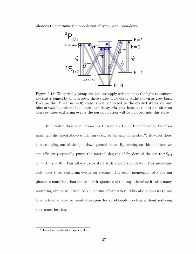
Figure 2.13: To optically pump the ions we apply sidebands to the light to connectthe states joined by blue arrows, these states have decay paths shown as grey bars.Because the |F = 0,mf = 0〉 state is not connected to the excited states via anyblue arrows but the excited states can decay, via grey bars, to this state; after onaverage three scattering events the ion population will be pumped into this state.
To initialize these populations, we turn on a 2.105 GHz sideband on the reso-
nant light discussed above which can decay to the spin-down state6. However there
is no coupling out of the spin-down ground state. By turning on this sideband we
can efficiently optically pump the internal degrees of freedom of the ion to 2S1/2
|F = 0,mF = 0〉. This allows us to start with a pure spin state. This procedure
only takes three scattering events on average. The recoil momentum of a 369 nm
photon is much less than the secular frequencies of the trap, therefore it takes many
scattering events to introduce a quantum of excitation. This also allows us to use
this technique later to reinitialize spins for sub-Doppler cooling without inducing
very much heating.
6Described in detail in section 3.2.
27

0 2 4 6 8 10
time (µs)
0.0
0.2
0.4
0.6
0.8
1.0
Prob. ↑
Figure 2.14: Average florescence of an ion as we gradually increase the time wepulse on the frequency sidebands for optical pumping. As this time is increased itbecomes more likely that the ion will decay to the |F = 0,mf = 0〉 state and nolonger scatter any photons, this is seen in the decrease in ion florescence observedat longer times.
28

Chapter 3: Experimental Apparatus
The experimental apparatus can be broken down into several parts: the vac-
uum chamber, which is used to trap and store ions. The optics, which are used to
trap and laser cool ions, as well as collect the light scattered from the ions during
detection. The Raman laser, which drives coherent operations between the clock
states of the ions. Finally, the electronics and control system which orchestrates the
interplay of all of the dynamical process introduced by the other systems. In this
chapter I will go over each of these systems and their sub-systems in detail.
3.1 Vacuum Chamber
A fundamental limitation to the number of ions in an experiment that one can
achieve in a trapped ion quantum simulator or quantum information processor is
fundamentally linked to the quality of the vacuum in the chamber that houses the ion
trap. The longer the ion chain is, the higher the probability of collisions occurring
with background gases. When there is more than one ion in the trap, re-cooling
from such collisions can be extremely difficult because the ions push each other into
orbits of the trap which can actually drive ion motion non-conservatively until ions
begin to exit the trap. Usually when these collisions occur in large ion chains, the
29

ion loss is catastrophic, resulting in only a single trapped ion after re-cooling.
Because of this, the trade off between the length of an experiment and the
length of the ion chain being used are strongly dependent on the quality of the
vacuum chamber. It is therefore paramount to achieve the best vacuum possible,
vacuum pressures commonly achieved are in the low 10−11 Torr range. This regime
is known as ultra-high vacuum (UHV), and achieving this level of vacuum requires a
great deal of care when assembling the vacuum chamber. Most importantly, before
any component is introduced to the vacuum side of the chamber it undergoes a
rigorous cleaning procedure.
In the case of the vacuum chamber discussed in this thesis this process con-
sisted of an ultra-sonic cleaning of all parts first in a bath of SimpleGreen and water,
to remove excess greases and hydrocarbons, followed by a bath of spectroscopic grade
acetone and finished with a bath of methanol. Once assembled the chamber was
baked, with blank steel flanges in place of the vacuum windows, at 200C for two
weeks. At this point the chamber was cooled down to room temperature, the trap
and windows were installed, and the chamber was baked again at 200C for eight
hours followed by two weeks at 180C1.
3.1.1 External Chamber Components
All external components are joined with metal to metal seals. In most cases
this means a ConFlat (CF) seal. This seal consists of two stainless steel “knife-
1This was done to be sure that surface effects would not damage the trap. For example ifthere was any pinned Aluminum in the trap would not grow ‘whiskers’, needles of Aluminum thatgrow out the planar surface, these ’whiskers’ can break through ground layers of the trap shortingvarious trapping components. This is less of a concern for the trap we are currently using.
30

Figure 3.1: CAD model of the vacuum chamber, labeling all of the relevant externalcontrols.
edges” on either side of the seal compressed into a copper gasket. This permanently
deforms the gasket to form the seal, and the chamber consists of many of these
CF components. The trap itself sits in the “spherical octagon” and all the wires
necessary for controlling a micro-fabricated trap exits through the 90 elbow on the
bottom 4.5” flange of the octagon. These wire are then routed out of the vacuum
chamber by D-sub connectors on the 4.5” four-way cross. Each feed-through flange
supports 50 wiring connections.
This four-way cross is attached to a five-wave cross that connects to all the
pumps and any additional feed-throughs. On the top of the cross is a 20 l/s ion pump
used to maintain the UHV conditions. On the bottom left there are connections to
31

an NEG cartridge from SAES (CapaciTorr D 400-2). This pump is made of sintered
porous Zr-V-Fe alloy disks which have high pumping rates for Hydrogen gas as
well as active gases. Opposite the getter is a three-way cross which houses a nude
UHV ion gauge to measure the vacuum pressure in the chamber and a Titanium
sublimation pump, which works by coating the inside walls of the chamber with
Titanium, which is a very good getter.
At the back of the cross there is another 2.75” tee which we use to attach a high
current feedthrough for the oven connections. This tee is also used to attach an all-
metal valve which we open during the bake out procedure to pump out the chamber
with mechanical pumps. This is necessary when the chamber reaches atmosphere,
because the internal pumps cannot handle a large gas load. When cooling down
the oven during the bake out procedure we seal this value and turn on the internal
pumps. The valve has a CF gasket internally which is pressed into a “knife-edge”.
If this is done consistently at the appropriate torque this gasket is re-sealable. The
decision to make everything 4.5” in diameter was made to maximize the conductance
to the internal ion pump and any external pumps used for baking the system.
3.1.2 Internal Chamber Components
All internal components are chosen to have as low of an out-gassing rate as
possible, and whenever possible we refrained from using components which are com-
prised of organic or porous materials. Organics, like plastics, tend to have worse
out-gassing rates compared with properly cleaned ceramics or metals. Porous ma-
32

terials can and will absorb the solvents used to clean them and then re-emit them
under vacuum conditions, which will limit the ultimate vacuum pressure achieved.
The internals of the vacuum chamber consist almost entirely of a wiring harness
that takes the connections from the trap electrodes to outside of vacuum.
In the spherical octagon, there are two groove grabbers that secure the stainless
steel wiring harness to the octagon. The trap assembly is plugged into a polyether
ether ketone (PEEK) socket, which is itself mounted to the wiring harness. All of
the 98 DC connections are routed out from the socket with 22 AWG kapton coated
wires; the RF connections2 are also made through this socket, however they are
directly routed out of the vacuum chamber via a 1.33” feed-through on the octagon
to minimize the length of the RF line. The socket is formed by two pieces of custom
machined PEEK, which captures 100 gold plated sockets that are crimped to the
ends of kapton wires. The PEEK has holes oriented so that a standard ceramic pin-
grid array (CPGA) can plug into the captured sockets. The trap that is discussed
in this thesis only has 48 DC electrodes, but this socket configuration is standard
across current ion trap foundries. In principle any micro-fabricated trap currently
available from GTRI, Honeywell, or Sandia can be plugged into this socket.
Besides the trap, the other major component internal to the vacuum chamber
is the Yb oven. We use an isotoptically enriched source of Yb that was purchased
from Oak Ridge National Labs. The oven is constructed from a tube of stainless
steel; one end of the tube is crimped shut and the other end is open. There are
2The RF lines constitute a current carrying wire and the current return which is connected tothe chamber at the resonator and to the ground plane of the chip.
33

Figure 3.2: Schematic of the oven, the oven is set back from the trap by approxi-mately 1 inch, the oven is an open aperture that sprays neutral Yb at the trap. Thesmall slot through the trap lets a relatively collimated beam of Yb into the trappingregion. The oven is supported by two stiff stainless steel wires of diameter 20 mil.
stainless steel wires spot welded to the exterior of the tube at either end, these
wires are bent to hold up the oven assembly. Each wire is wound around a gold
plated screw attached to a metal block; a kapton wire also attaches to the block and
is routed out of the vacuum chamber via a high current feed through. These wires
constitute the current and current return for the oven. When current is run through
the tube, it is resistively heated and sublimated Yb can exit the opening at the top
of the oven. This oven is pointed so that atom flux will be perpendicular to the trap
plane and directed at a small slot cut into the trap which will allow atoms to pass
through the trapping structure. The backside of the trap is coated with a grounding
layer and the gaps in-between electrodes are undercut to avoid sublimated Yb from
shorting the trap. This assembly is held by the stainless steel blocks which bolt
34
around macor rods attached to the metal wiring harness, which allows the oven to
be thermally and electrically isolated from the rest of the chamber.
3.2 Optics
Almost all of the available adjustable parameters in this experiment are op-
tical. All the interrogation of atoms is done with lasers, and our ability to discern
anything about the atomic quantum states is determined by collected the light which
is scattered from them. Which is to say that this piece of the experimental appara-
tus is one is which we need the highest degree of accuracy and control. There are
three main tasks for which we use optical elements: ionize and the Doppler cool3 the
ions in the trap, image the light scattered from the ions to determine information
about their internal degrees of freedom4, and finally interrogate ions with laser light
to manipulate their internal degrees of freedom5. The following subsections will
describe the physical systems that achieve these tasks.
3.2.1 Cooling and Trapping Beam Paths
The Doppler cooling and ionization light is generated by external cavity diode
lasers. The 399 nm and 935 nm lasers are DL 100 Toptica lasers, and the 369 nm
laser was produced by MogLabs. The final laser we have is a 780 nm DBR laser
which is locked via a saturated absorption lock to a Rb spectroscopy cell. The 780
nm light provides a stable reference for a WSU-2 wavemeter from High Finesse.
3The theory of this is discussed in section 2.3.24The theory of this is discussed in section 2.3.35The theory of this is discussed in section 4.1.1
35

This wavemeter is then used to lock the frequencies of the other lasers.
Figure 3.3: Optics for the the 399 nm laser the light is split out to a wavemeter toread the frequency, a cavity to lock the frequency, and finally to the chamber to beused as the first stage in photoionization
The 399 nm beam path is the most straight forward, and consists of an optical
isolator followed by several pelical beam splitters to route the light into various fiber
couplers. There is a coupler for a cavity locking setup, which in the future will be
used along with the other lasers in a scanning transfer cavity lock 6. Another coupler
brings approximately 20 µW of power to the wavemeter currently being used to lock
frequencies. An additional 700-900 µW of power is fiber coupled to the chamber.
Once at the chamber, the beam is focused to approximately w0 = 70µ m and is
directed perpendicular to the axial trapping direction, z. The beam is then raised
60 µm to address atoms as they pass through the loading slot and cross the trapping
region.
The 935 nm laser is our 2D3/2 state re-pump laser, and also has a relatively
simple beam path. The laser passes through an optical isolator and then is split
into three arms see Fig 3.4, each going to the same assemblies as the 399 nm arms,
6See Appendix A for a more detailed discussion of locking schemes.
36

as seen in Fig 3.3. The only difference is the light that gets directed to the chamber
first passes through a 3.086 GHz free space electro optical modulator (EOM) from
New Focus. This EOM introduces frequency sidebands on the light by modulating
the index of refraction of an internal crystal at an applied RF driving frequency.
Light passing through the crystal experiences shifts in the index of refraction at
this RF oscillation frequency, this imparts a time dependent phase shift to the
light, E(t) = E0ei(ω0t+β cos(ωRF t). If we expand this in Bessel functions we get an
electric feild of the form, E(t) = E0
(J0(β)eiω0t + J1(β)ei(ω0+ωRF )t − J1(β)ei(ω0−ωRF )t
)[38]. This imparts frequency sidebands to the light at the drive frequency with a
modulation depth dependent on the applied RF voltage. This modulation allows us
to use one laser to re-pump all of the possible hyperfine states coupled between the
D3/2 and the [3/2]1/2 bracket state.
Figure 3.4: Optical setup for the 935 nm light The addition of the EOM is the onlydifference from the 399 nm beam path, this EOM is from NewFocus and is used tobridge the hyperfine splittings of the D3/2 and [3/2]1/2 states.
The final laser system is far more complicated. This is maybe unsurprising, as
this is the laser used to ionize, cool, and detect the spin state of the trapped ions.
The 369 nm laser is also a direct diode laser, it passes through an optical isolator at
37

which point it is split into two paths, one that is subsequently split again to send
power to both the cavity as well as the wavemeter. The amount of power sent to
these paths is controlled by a waveplate and is varied to minimize the amount of
power directed to these arms.
Figure 3.5: Optical setup for the 369 nm laser. The 369 beam path is the mostinvolved, this path involves two acousto optical modulators (AOM) and two EOMs.Both AOMs are from Brimrose and the EOMs are from NewFocus. The 7.14 GHzEOM is to impart sidebands to drive all possible transitions to scatter the maximumnumber of photons during cooling. The 2.105 GHz EOM is used to optically pumpthe ions to the |F = 0,mf = 0〉 ground state.
The remaining power is split between two arms via polarizing beam splitter.
One arm passes through a 7.379 GHz free space EOM, from New Focus. This EOM
provides second order frequency sidebands at 14.758 GHz, the qubit splitting, 12.65
GHz, plus the hyperfine splitting of the 2P1/2 excited state, 2.105 GHz. This arm
is our Doppler cooling arm. These sidebands allow us to scatter photons from all
ground states7. Once light passes through this EOM, it is directed towards a double-
7Discussed further in Chapter 2
38

passed acousto-optical modulator (AOM). We use a double pass configuration to
shift the frequency of the beam without shifting its position.
S1/22
P1/22
F=1
F=1
F=0
F=012.64 GHz
2.105 GHz
Figure 3.6: Re-print from section 2.3.2 for ease of reference. To scatter as manyphotons as possible we send in light with all polarization components and apply side-bands to the 369 nm light to bridge the ground and excited state hyperfine splitting.The blue arrows represent the states connected via dipole allowed transitions drivenby laser light. The grey bars represent the possible spontaneous decay paths fromthose excited states.
The AOM works by applying a running acoustic wave to an internal crystal,
whcih diffracts light as it passes through the AOM. The light will absorb the mo-
mentum, ±kacoustic, shifting the propagation direction and shifting the frequency
of the light to maintain energy conservation. Our 369 nm AOM systems are set up
to maximize the -1 order of diffraction. This beam is then sent through a λ4
wave-
plate and onto a mirror at normal incidence. The light then passes back through
the whole assembly. The frequency of the light is shifted by twice the AOM drive
frequency but is not shifted in position. We set the frequency shift such that we are
red detuned from the 2S1/2 ↔2 P1/2 transition by 10 MHz for Doppler cooling the
ions. However, in the double-pass configuration we have the ability to easily tune
this frequency. Once the light hits the PBS that was directing it towards the AOM
39

the polarization has been rotated 90 by passing through the λ4
waveplate twice.
The beam then passes or reflects where previously it reflected or passed. This is a
common place technique in atomic physics experiments where the frequency of light
needs to be controlled quickly without affecting the final position of a beam.
170 175 180 185 190 195 2002
0
2
4
6
8
10
12
14
16M
ean P
hoto
n C
ounts
ωAOM(MHz)
Figure 3.7: Scattered phtons from the S1/2 → P1/2 transition as a function of theAOM frequency. By scanning the frequency of the detection AOM, we can scan theS1/2 → P1/2 transition to determine where to tune the AOM frequency to maximizescattered photons.
The other arm is similarly directed onto a free space EOM from New Focus,
operated at 2.105 GHz. This EOM, which we pulse on and off during the course of
an experiment, applies a sideband to the light at the hyperfine splitting of the 2P1/2
excited state. From this state the ion can decay to both the |F = 1〉 and |F = 0〉
ground state manifolds. This light will couple the |F = 1〉 ground state manifold to
the excited 2P1/2 state but does not couple the |F = 0〉 ground state to the excited
state, because this state is detuned by 12.64 GHz8. This sideband optically pumps
the ion spin state to the |F = 0〉 ground state, this is how we initialize the spin state
8Discussed in depth in section 2.3
40

of our ions.
S1/22
P1/22
F=1
F=1
F=0
F=012.64 GHz
2.105 GHz
Figure 3.8: Atomic energy levels used to initialize the ion in a pure spin state wemake use of the hyperfine splitting in the ground state, we can decouple it entirelyfrom the resonate excitations of the upper hyperfine manifold. By scattering off theF=1 manifold depicted in blue, ions can decay via the grey pathways to the F=0ground state manifold, thus pumping the ion to the |F = 0,mF = 0〉 state.
This beam without the sideband works as our detection beam. When this side-
band is off, the light is resonant with the 2S1/2 |F = 1,mF = 0〉 ↔ 2P1/2 |F = 0,mF = 0〉
transition. The decay of this excited state has zero overlap with the 2S1/2 |F = 0,mF = 0〉
ground state, due to angular momentum selection rules. Therefore we can scatter
many photons from this spin state before it exits our qubit spin basis. This arm
also passes through an AOM which we use to shift the frequency of this transition
to optimize scattering. Once it has exited the AOM setup it is recombined with the
cooling beam on a PBS. Both beams are then directed onto the same fiber and sent
to the chamber.
Once at the chamber the light is split into two arms, each arm contains cooling,
pumping, and detection light. Each arm is focused down to approximately 30 µm
and is directed at 45 to the axial trapping direction, z, to give an overlap with all
41

S1/22
P1/22
F=1
F=1
F=0
F=012.64 GHz
2.105 GHz
Figure 3.9: Atomic energy levels used for detecting the spin state of the ion. Thegray line shows the possible decay paths and one can see that there is no connectionto the spin down state.
principal axes of the trap. One arm of this light is directed towards the loading zone
of the trap and the other is directed to the region where we couple the ions to the
Raman laser, these regions are separated by 250 µm.
3.2.2 Imaging system
To determine the spin state of ions, as previously described, we scatter photons
off of the 2S1/2 ↔ 2P1/2 transition. We then need to collect the scattered photons,
the more photons we collect the higher our confidence will be in the spin state
discrimination. This is complicated by off resonant coupling to the 2P1/2 |F = 1〉
manifold, which can scatter back to the 2S1/2 |F = 0〉 ground state manifold. For
fixed laser power and detuning, the longer we attempt to collect scattered pho-
tons, the higher the probability we will off resonantly scatter to the 2S1/2 |F = 0〉
ground state. Therefore, the faster or the more photons we collect the better the
discrimination will be between the spin-up and spin-down states.
42

0 5 10 15 20 25 300.0
0.1
0.2
0.3
0.4
0.5
0.6
0.7
Dark IonBright Ion
Figure 3.10: Histograms of collected photons when illuminated for 200 µs. Thered bars, in which we collected 15 average photons, indicates this ion is bright. Theblue bars indicates a dark ion. The intermediate photon numbers is indicative of thecross talk we see between PMT channels. This histogram was taken with multipleions in different spin states in the trap. The shelf of low photon counts for the brightion is indicative of off resonant pumping to the 2S1/2 |F = 0〉 ground state.
Figure 3.11: Optical layout for the ion imaging system. The first set of 5 lenses is amulti-element objective that has a working distance of approximately 25 mm and anNA of 0.4, corrected for the vacuum chamber window thickness. The intermediateimage plane is focused back to either a mutli-channel PMT or a camera to imageions. The final cylindrical lens is used to correct for astigmatism in the lens stack.The distance between the two final spots shows the displacement of the imagesformed by two ions separated by 50 µm at the trap yielding a magnification of 276
To collect photons we employ a multi-element objective which has an NA≈ 0.4
and a working distance of WD ≈ 25.8 mm. This objective forms an image plane 215
mm back from its last surface. This intermediate image is re-imaged with a doublet
of two LBF254-040-A f = 40 mm best form lenses from Thorlabs. This doublet forms
43

4000.0
0
OBJ: 0.0000 mm
IMA: 0.000 mm
OBJ: 0.0500 mm
IMA: 13.806 mm
OBJ: 0.0015 mm
IMA: 0.414 mm
Airy Radius: 116.6 µm
RMS radius : 427.802 427.912 537.938
Figure 3.12: Spot diagrams for object ions separated perpendicular to the imagingaxis. The purpose of this simulation is to determine what aberrations are inducedby trying to image more than one position of the trap simultaneously. Diagram (a)shows the central ion, the black ring shows the Airy radius. The next spot diagramis for an ion displaced by 1.5 µm from the first ion, a close adjacent ion in the trap.The (c) image shows an ion displaced by 50 µm, the maximum distance we expectto have an ion if we trap the largest chain we can image. The other important thingto note is that the RMS radius of each spot is approximately 0.5 mm. This impliesthat well imaged ions should fit on a single PMT channel.
an image onto a multi-channel PMT 680 mm back. The multi-channel PMT has
channels spaced by 1 mm, and the measured overall magnification of this systems is
M ≈ 200, there is a small discrepancy between the simulated and measured values9.
This requires the ions to be spaced by at least 5 µm for individual detection, and
in practice we use our ability to deform the axial potentials to space the ions out
by at least 10 µm so that there is a dead channel in-between channels imaging ions.
This reduces cross talk on the multi-channel PMT.
9This is measured by imaging trap features onto a scientific CMOS camera with known pixelsize.
44

3.2.3 Raman Beam Path
The beam path for the Raman laser is the most critical, since the intensity of
this beam directly affects the coherence of our qubit transitions10. We use a Paladin
Compact pulsed NdYag laser from Coherent to generate these beams. This laser
is a tripled 1064 pulsed laser, and is used commercially for photo lithography in
semi-conductor fabrication facilities. Immediately out of the laser, a beam sampler
directs a small portion of the light onto a fast photodiode to measure the repetition
rate of the laser. We bridge the hyperfine transition by combining two pulse trains
of this laser and interfering two comb teeth, generating a beatnote at the qubit
splitting. This is followed by an AOM, which we use to stabilize the intensity of the
laser. The non-diffracted order of this AOM is sampled by a pick-off mirror with
very low reflectivity. The sampled light is then directed onto a slow photodiode to
generate an error signal to feed back to the AOM power for stabilizing the amplitude
of the pulse.
The beam is then split into two arms and focused down onto two AOMs. One
of these AOMs is used as a feed forward control of the repetetion rate of the later11.
The other is used to scan the frequency of the beatnote or apply multiple frequency
components to this beatnote. By focusing the beam down onto these AOMs, we
can use lenses afters the AOMs to image the waist formed in the AOM onto the
ions. We do this so that frequency shifts do not result in beam translations at the
ions. We collimate the diffracted orders out of each AOM,and pick off the +1 order
10Discussed further in Chapter 4.1.11This will be discussed more fully in section 3.3.3.
45

Figure 3.13: Raman beam paths to the chamber. The total path length is approx-imately 3 meters. The majority of this system is enclosed in beam tubes, whichare in turn enclosed in a box constructed of 80/20 Allucabest panels. The reasonfor this is two fold: it protects people in lab from the UV light and helps preventair currents from passing through the beam path. These air currents can causegradients in the index of refraction in air and lead to pointing instability.
on a D-shaped mirror. One of these arms is directly sent to the chamber via a
periscope, while the other arm passes through a variable delay stage. The delay
stage is necessary to make sure that the pulses overlap temporally and spatially at
the ion chain. Because we split the beam into two arms this delay stage acts to
make the arms equal length.
Before these beams are focused down onto the ions, they pass through PBS
cubes to achieve a clean horizontal polarization. At the ions, the beams are per-
46

Figure 3.14: Beam paths for all of the lasers as they enter the vacuum chamber.
pendicular to each other and parallel to the trap surface. With the magnetic field
defining a quantization axis pointing perpendicular to the trap surface, this satisfies
the lin ⊥ lin configuration [39] of polarization needed to drive Raman transitions12
in 171Yb+. Both beams are focused down with an f = 100 mm UV fused silica lens
from Thorlabs, this results in beam waists of approximately 40 µm. These beams
are oriented so that the δk of the two beams points parallel to the trap surface and
along a direction perpendicular to the axial trapping direction. This lets us induce
momentum transfer between the beatnote and the ion chain along only one of the
transverse trapping directions13.
Because of its commercial applications, this laser is almost entirely turn-key
12Discussed in depth in Chapter 4.1.2.13Discussed in depth in section 4.1.3.
47

Figure 3.15: The direction of the k vectors of the Raman beams at the trap, withthe relevant directions of the trap axes and magnetic field axes also defined.
and there is very little that the user has in the way of control. Unsurprisingly this is
insufficient for our purposes. In particular, the cavity that generates the pulse train
is totally inaccessible, and changes length over time which changes the spectrum
of the frequency comb emitted. The repetition rates of these lasers is typically
in the 80 MHz or 120 MHz range, where the exact frequency is variable laser to
laser. To bridge the hyperfine splitting at 12.64 GHz, we must interfere two comb
teeth separated by approximately 105 comb lines. That means 10 kHz shifts of the
repetition rate change our beatnote frequency by MHz. Because we have no control
over the length of this cavity, we must feed forward to a frequency modulator after
the laser. I will discuss this stabilization circuit in depth in section 3.3.3.
48

3.3 Control Electronics
The final piece of the experimental apparatus not discussed so far are the
control electronics. These can be broken down into electronics used to control the
timing of operations in an experiment, the control over the DC and RF trapping
voltages, and the electronics used to stabilize all the various parameters in the
experiment which are not passively stable enough for our purposes.
Figure 3.16: Illustration of the control structure, depicting all of the digital elec-tronics used to control this experiment.
3.3.1 Timing Control
The timing control for our experiment is orchestrated by an Opal Kelly XEM6010-
LX150 FPGA. This timing FPGA is clocked at 100 MHz, from an atomic Rb source,
and is loaded with firmware developed as part of the Sandia ion control system.
49

This firmware allows us to write python like pulse programs that support “for” and
“while” loop functionality as well as conditional branching of the experimental pro-
cedure. This functionality allows us to perform complex experimental procedures.
We will take full advantage of this to do state distillation, which requires adapting
the experimental procedure during the course of the experiment, depending on feed-
back from the ion. This is achieved by sending the timing FPGA multiple branches
for all possible future operations. Because the experimental time scale of 10’s of
µs this approach is preferable to sending new commands to the timing FPGA dur-
ing an experiment. Such communications would be difficult to achieve with the
asynchronous communication between the PC and the timing FPGA.
In addition to timing control, this FPGA also controls a handful of peripherals
used in pulse programs. The parameters of these devices can be updated on the fly
during the experimental procedure. These devices include 8 AD 9912 DDS chips,
8 DAC8568 digital to analog converters, 8 AD7606 analog to digital converters, as
well as 24 digital inputs. We use these digital inputs to read in the signals from
the muli-channel PMT. The current system takes low voltage differential signals
(LVDS) from the multi-channel PMT’s individual channels to a separate Opal Kelly
XEM6010-LX45 FPGA. This PMT FPGA emits TTL pulses on a digital line back
to the timing FPGA for each LVDS signal. In the future, we plan to send back the
number of LVDS counts received on all PMT channels through serial communication
with the timing FPGA. This will be done over the same digital lines currently being
used, this is why the task of translating LVDS to TTL signal is currently performed
by an FPGA. In the future this PMT FPGA will be necessary to implement the
50

logic to determine what serial command to communicate back to the timing FPGA.
This configuration of FPGAs allows the timing FPGA to get back photon
count values, collected during the course of an experiment, on experimental time
scales. That means the timing FPGA can be programmed with conditional logic
that selects the next branch of operations based on returned photon counts. This
allows us to perform feedback to the operational parameters during the course of an
experiment.
The same digital lines are also used to communicate with another FPGA that
controls the DC voltages, this is done so that we can change the voltages during the
course of an experiment. This allows us to move and manipulate the ion position
during an experiment, this is necessary for our individual addressing scheme [40].
3.3.2 Trapping Voltage Control
Generating and controlling both the DC and RF trapping voltages is probably
the most challenging component of the experimental apparatus. The difficulties
in producing stable, low noise DC lines and a stable RF line are distinct. The
trouble with the DC lines arises from the sheer number of electrodes which must
be controlled and filtered without compromising their dynamic performance. The
challenges with the RF arise from the high voltage necessary and intrinsic reactance
of the components making up the line into the vacuum chamber. Because of these
differences, we will address each separately in the next two subsections.
51
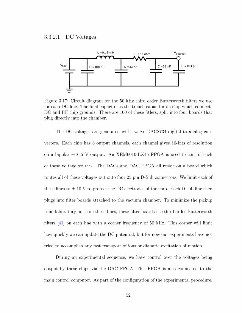
3.3.2.1 DC Voltages
C =100 nF C =33 nF C =33 nF
R =63 ohmL =0.15 mH
C =103 pF
Velectrode
VDAC
Figure 3.17: Circuit diagram for the 50 kHz third order Butterworth filters we usefor each DC line. The final capacitor is the trench capacitor on chip which connectsDC and RF chip grounds. There are 100 of these fitlers, split into four boards thatplug directly into the chamber.
The DC voltages are generated with twelve DAC8734 digital to analog con-
verters. Each chip has 8 output channels, each channel gives 16-bits of resolution
on a bipolar ±16.5 V output. An XEM6010-LX45 FPGA is used to control each
of these voltage sources. The DACs and DAC FPGA all reside on a board which
routes all of these voltages out onto four 25 pin D-Sub connectors. We limit each of
these lines to ± 10 V to protect the DC electrodes of the trap. Each D-sub line then
plugs into filter boards attached to the vacuum chamber. To minimize the pickup
from laboratory noise on these lines, these filter boards use third order Butterworth
filters [41] on each line with a corner frequency of 50 kHz. This corner will limit
how quickly we can update the DC potential, but for now our experiments have not
tried to accomplish any fast transport of ions or diabatic excitation of motion.
During an experimental sequence, we have control over the voltages being
output by these chips via the DAC FPGA. This FPGA is also connected to the
main control computer. As part of the configuration of the experimental procedure,
52

1.000 10.00 100.0 1.000k 10.00k 100.0k 1.000M 10.00M 100.0MFrequency (Hz)
(dB
)
-250.0
-212.5
-175.0
-137.5
-100.0
-62.50
-25.00
12.50
50.00 dB(in)
dB(out) for RC
dB(out) for Butterworth
Figure 3.18: Simulated filter function for the Butterworth filters we use, the knee issomewhat softened by the intrinsic resistance of the inductor.
we define a large array of voltages for each DC line. These voltages correspond to
simulated solutions to the DC potential along the axial trapping direction, z. These
simulations are based on Green’s functions of the trap geometry. The simulations
are performed by the trap designers and we have very limited access to the codes
they use to do these simulations. We then specially define the specific solutions
where we perform experimental procedure. These include specific positions along
the trap, as well as solutions which change ion spacing, or add anharmonic terms
to the DC potential. In general we have to get these specific solution types, once
specified, from the designers of the trap. When the simulations are run we get
specific solutions as well as the array voltages necessary to move between these
specific solutions. One can picture these particular solutions as nodes in a graph,
with the array defining the edges between nodes. By defining a graph in this way,
we have a map between different points of interest.
As part of the configuration of these voltage nodes we define the rate at which
voltages in the array should be applied to move from one node to another. We
53

also define the interpolation between lines in this array, as well as any wait times
to be executed as each line of the array is applied. When the nodes are defined,
they are loaded with the array of edges into the memory of the DAC FPGA. The
DAC FPGA and the main timing FPGA are connected via digital I/O lines of
the main timing FPGA. When an experiment is initialized on the PC side the two
FPGA’s synchronize. To manipulate the ions during an experiment, the timing
FPGA sends a serial command to the DAC FPGA that tells the DAC FPGA which
edge between operational nodes to execute. The timing FPGA then waits for a signal
from the DAC FPGA signaling completion of this operation before it continues with
the experimental procedure. This “handshake” synchronization between FPGAs is
sufficient for our purposes.
3.3.2.2 RF Voltage
The RF voltage applied to the trap is generated by an HP ESG-1000A source
amplified and then filtered by a helical resonator [42]. The challenging aspect of
generating this RF voltage is that the voltage at the trap is directly proportional to
the secular frequencies of the trap, and the frequency must be clean enough to not
drive secular motion of the trap14. Because of this second issue, we generally use
quarter wave resonators to transform power to voltage on the open voltage node of
the trap.
This resonator functions by coupling a source coil to a larger coil whose length
is approximately one quarter of the desired RF drive wavelength. The end of the coil
14Discussed in depth in section 2.1.1.
54

Figure 3.19: A cross section of the helical resonator used to step up the RF powerto voltage to drive the transverse confinement of the trap.
near the source is grounded to the housing of the resonator, which has cylindrical
symmetry. The other end of the coil is then connected to a feedthrough which is
connected in vacuum to the RF rail on the chip. This end of the coil is an anti-node
of the standing wave present in the resonator. By moving the source inductor in and
out of the larger coil, we can change the coupling impedance between the two. On
resonance, these circuits can have high quality factors Q = Ω0
ω∆, where ω∆ is the full
width half maximum frequency of the resonator and Ω0 is the resonance frequency of
the resonator. For our resonator, the drive frequency is Ω0 = 35MHz and Q ≈ 200.
Since the secular frequencies of our trap are usually in the 1-3 MHz range, this is
adequate spectral purity for the experiments we wish to perform. The bigger issue
for our experiment is trying to maintain a stable RF voltage at the trap, this will
be discussed in the next section.
55

3.3.3 Stabilization
Due to the sensitive nature of these experiments a handful of parameters must
be controlled actively. The two which are the most important are the RF voltage and
the beatnote frequency of the Raman laser. As previously stated the RF voltage in
directly proportional to mode frequency. Therefore, this voltage must be stabilized
or the coherence of a transition coupled via the motion will be strongly degraded.
LO
RFIF
PID
Ctrap
Rectifier
Helical Resonator
2 K
68 pF
5 KHMPS2822
5 Kf=36.17 MHz
Amp
Lcoupler
Lcoil
HMPS2822
0.2 pF
5.6 pF
Figure 3.20: The lumped element circuit model of the resonate circuit used to stepup the RF voltage for the trap.
The difficulty with stabilizing this signal is that it is high voltage at radio
frequency, derived from a resonate circuit. Any dissipative elements used to sample
the voltage will destroy the resonator quality factor. Because of this we use reactive
elements, specifically a capacitive voltage divider to sample the high voltage anti-
node of the resonator. If appropriate capacitors are chosen, the ratio of trap voltage
tap voltage can be stable to a few parts per million. In our experiment, the ratio
of trap voltage to tap voltage was measured to be 178. This signal is then sent
into a rectifier to turn this RF signal into a DC error signal. Once we have a DC
56

signal proportional to the RF amplitude, we feed this into a feedback loop [43].
Both the rectifier and the capacitive tap use very low thermal coefficient, passive
components. The error signal is then sent into an off the shelf servo controller,
NewFocus LB1500. We extensively test this feedback by measuring the stability of
the secular frequencies. The context in which we took this data and its implications
to our experimental goals are discussed in Chapter 6.
As stated previously, we interfere two comb teeth of our pulsed laser to create a
beatnote at the qubit splitting to drive all the coherent operations detailed through-
out this thesis. The beatnote must be stabilized because, as previously stated, the
internal laser cavity that is generating these pulses is not actively stabilized. Be-
cause the length of this cavity directly determines the repetition rate of the laser, if
environmental factors can couple into the length of this cavity, they can affect the
beatnote frequency. Unfortunately, our laser does not provide any external control
of this cavity length so it cannot be directly stabilized. However, because the beat-
note driving our Raman transitions is derived from two beams split from the same
source we can use an AOM to compensate for drifts in the repetition rate. This
feedforward method of stabilizing the beatnote is very similar to the stabilization
used in a phase locked loop (PLL).
To accomplish this lock, we sample the beam directly out of the laser and
measure, with a fast photodiode from Alphalas, the frequency comb of the laser. By
amplifying and filtering this comb we can isolate the specific comb line which will
participate in driving Raman transitions. We then mix this comb line down with
a stable frequency source. This source also acts as the global clock for all coherent
57

LORFIFBPF
LORF
IFPID
FM
AOM
f f
ff=12.74 GHz
f=80 MHz
From Raman Laser
Figure 3.21: A schematic for the feed forward lock used to stabilize drifts in therepetition rate of the 355 laser. We use an HP 8672 for the microwave source andan HP 8640 for the AOM drive. The bandpass filter is a 12 pole waveguide filterwhich I optimized for the comb line of interest. It has a bandwidth of approximately100 MHz and a center frequency of 12.8 GHz.
operations and therefore is referenced to a stable Rb clock. The demodulated beat-
note signal, which is around 79 MHz, is then mixed with the source used to drive
the AOM at approximately the same frequency. The resulting DC signal is fed into
another servo (NewFocus LB1500). The feedback is applied to the frequency mod-
ulation port of the source driving the AOM. This allows us to remove shifts in the
repetition rate of the laser before the light reaches the ions [44,45].
3.4 Ball Grid Array Trap
The trap we used to do all of the experiments discussed here was developed in a
collaboration between Honeywell and the Georgia Tech Research Institute (GTRI).
The trap is known officially as the ball grid array (BGA) trap and implements a
relatively simple linear trap design. The trap is gold on a silicon substrate, the ions
when trapped sit approximately 60 µm from the surface of the trap. There are 48
58

Figure 3.22: A schematic of the trap structure, the smaller DC electrodes in pink are60 µm apart, the larger DC electrodes near the loading zone are 100 µm wide. Theloading slot is approximately 60 µm wide. There are large DC electrodes aroundthe periphery of the trap to help rotate the DC axes if necessary.
DC electrodes, 60 µm in width each, a slot for loading ions from the backside, and
a specified ion to RF electrode distance of 94 µm. GTRI designed the trap and
Honeywell fabricated the trap. The intent was to create a trap with high optical
access. Because micro-fabricated traps are so small and the coupling between the
RF and DC electrodes can lead to pickup of RF on the DC electrodes, by having
small capacitors on-chip to mitigate this effect. This is a tradeoff, however, since
these capacitors take up real estate on the chip. If you want to focus down laser
beams to address individual ions, normally separated by no more than 5 µm, the
Rayleigh length of those beams will be quite short. This means that the trapping
structure itself can be the limiting factor when tightly focusing lasers above the
surface.
Groups have tried a variety of approaches to get around this difficulty. The
most popular of these approaches involves etching a slot through the chip which
can have very high NA from above the chip [46]. Another recent approach has
59

Figure 3.23: CAD model of the trap in the spherical octagon to give as sense ofscale for how close the trap is to nearby surfaces.
been to raise a relatively small trapping area above the carrier which routes the
electrical connections out to the ceramic pin grid array (CPGA) attached to the
wiring harness. To do this, however, you have to find a place to put all of the filtering
capacitors. This has led to the bow-tie like geometries of traps like the Sandia High
Optical Access (HOA) trap, as well as traps with some novel fabrication techniques
including our trap the BGA.
The BGA utilizes trench capacitors, which are located directly under each
electrode and go down to a ball which is bump bonded onto the carrier. This
configuration means the raised trapping structure can be very small. The BGA is
only 0.4× 1.1× 3.3 mm in extent, and the surface is essentially only populated with
the trapping electrodes. In principle this means that we can get tightly focused
60
beams across the surface, but this is not the case in practice due to an oversight in
design. The carrier which routes out electric connections is still too large, and the
trap is not tall enough. The smallest spot sizes we can achieve with our 355 nm
laser are approximately 8 µm.
In the future, we plan to move to the Sandia HOA trap which has both a high
NA≈ 0.2 from the side as well as a slot through the trap that has an NA≈ 0.6. This
will allow us to get beams focused down to 1 µm, at which point we should be able
to individually address ions in the chain.
61
Chapter 4: Coherent Operations
In this chapter I want to go through the atom-light interactions. To coherently
manipulate the spin state of the ions, we use stimulated Raman transitions. If we
so choose, we can align these beams to have a net δk momentum transfer along one
of the principal axes of the trap allowing us to couple to not only the spin degree of
freedom but also the external degrees of freedom.
4.1 Raman Interaction
Consider a three level atom described by two ground states |0〉,|1〉, and one
excited state |e〉. Leaving out the motion for a moment, choose the |0〉 as the zero
energy level, 〈0| H0 |0〉 = 0. Then we can write down an ion Hamiltonian of the
form,
H0 = hω1 |1〉 〈1|+ hωe |e〉 〈e| (4.1)
With an arbitrary wavefunction,
|ψ〉 = c0 |0〉+ c1 |1〉+ ce |e〉 (4.2)
62

To couple states |0〉 and |1〉 with light from two beams, the electric fields of
these beams takes the following form.
E1 =1
2E01e
−i(ωL1t+φ1) + h.c. (4.3)
=1
2E1ε1e
−i(ωL1t+φ1) + h.c. =1
2E1ΦL1ε1 + h.c. (4.4)
E2 =1
2E02e
−i(ωL2t+φ2) + h.c. (4.5)
=1
2E2ε2e
−i(ωL2t+φ2) + h.c. =1
2E2ΦL2ε2 + h.c. (4.6)
(4.7)
The vector amplitudes, E01 andE02, include a polarization vector, and the fre-
quencies of the beams are such that one laser couples |0〉 ↔ |e〉 with an arbitrary
detuning δ on top of a large detuning ∆0. The other laser couples |1〉 ↔ |e〉 with a
frequency similarly far detuned, minus the splitting between the two ground states
|1〉 and |0〉.
Explicitly, we have the frequencies, ωL1 = ωe+∆0−δ and ωL2 = ωe−ω1 +∆0.
We have also absorbed the position of the ions relative to the incident field into the
phases φ1,2; this position will allow us to couple to the external degrees of freedom
of the ion chain and will be discussed later in this chapter.
The coupling between states |0〉 ↔ |e〉 and |1〉 ↔ |e〉 is mediated by these two
beams, and takes the form of an electric dipole transition.
63

〈i| HI |e〉 = −〈i|µ ·Ej |e〉 (4.8)
= −〈i|µ · εj |e〉 Ej (4.9)
〈i|µi · εj |e〉 = 〈e|µi · ε∗j |i〉 (4.10)
µi · εj = µi,ejEj |i〉 〈e| (4.11)
µi · ε∗j = µ∗i,ejE∗j |i〉 〈e| (4.12)
Where µi,ej is related to a reduced dipole matrix element between states |i〉 and
|e〉 for the jth beam, Ej and εj are the electric field amplitude and the polarization
of the jth beam, we will look at these terms in depth in section 4.1.2. Equations
4.10-4.12 are a consequence of requiring Herminicity in the interaction Hamiltonian.
This gives us an atom-light interaction Hamiltonian of the following form,
HI = −µ ·E (4.13)
= − (µ0 + µ1) · (E2 +E1) (4.14)
= −1
2(µ0 + µ1) · (E2ΦL2ε2 + E1ΦL1ε1 + h.c.) (4.15)
where we have grouped all of the phases together in the terms Φi, and we have broken
out the individual polarization operators. We save the discussion of these parameters
for a later section detailing 171Yb+ specific parameters. Expanding equation 4.15,
we get
64

µ ·E =1
2(µ0 + µ1) · (E2ΦL2ε2 + E1ΦL1ε1 + h.c.) (4.16)
=1
2µ0 · (E1ΦL1ε1 + E∗1 Φ∗L1ε
∗1) +
1
2µ0 · (E2ΦL2ε2 + E∗2 Φ∗L2ε
∗2) (4.17)
+1
2µ1 · (E1ΦL1ε1 + E∗1 Φ∗L1ε
∗1) +
1
2µ1 · (E2ΦL2ε2 + E∗2 Φ∗L2ε
∗2)
(4.18)
To determine the population dynamics of an arbitrary state, we substitute
our interaction Hamiltonian into the Schrodinger equation, ihψ = Hψ = (H0 +
HI)ψ. For convenience we set h = 1 and solve the Schrodinger equation under some
simplifying assumptions. Solving for the individual probability amplitudes, ci, the
resulting time evolution is governed by,
ic0 = −1
2
(µ∗0e1E
∗1 Φ∗L1 + µ0e1E1ΦL1
)ce (4.19)
ic1 = ω1c1 −1
2(µ1e1E1ΦL1 + µ1e2E2ΦL2) ce (4.20)
ice = ωece −1
2
(µ∗0e1E
∗1 Φ∗L1 + µ∗0e2E
∗2 Φ∗L2
)c0 −
1
2
(µ∗1e1E
∗1 Φ∗L1 + µ∗1e2E
∗2 Φ∗L2
)c1 (4.21)
To make the following calculations a little less cumbersome, we will define the
single photon coupling rates for each of the transitions in the following way,
65

g0e1 = −µ0e1E1e−iφ1 (4.22)
g0e2 = −µ0e2E2e−iφ2 (4.23)
g1e1 = −µ1e1E1e−iφ1 (4.24)
g1e2 = −µ1e2E2e−iφ2 (4.25)
We can simplify the effects of multiple beams by writing the generalized cou-
pling as gikj = −µikjEje−iφj , where j is an index the beam, and i and k index the
coupled states. The coupled equations for the population dynamics then become,
ic0 =1
2
∑j=1
(g0eje
−iωLjt + g∗0ejeiωLjt
)ce (4.26)
ic1 = ω1c1 +1
2
∑j=1
(g1eje
−iωLjt + g∗1ejeiωLjt
)ce (4.27)
ice = ωece +1
2
∑j=1
[(g0eje
−iωLjt + g∗0ejeiωLjt
)c0 +
(g1eje
−iωLjt + g∗1ejeiωLjt
)c1
](4.28)
We can simplify these equations by moving to the frame rotating with respect
to the un-perturbed Hamiltonian. We apply the following transformation to our
system of coupled equations,
66

c0 = c0 (4.29)
c1 = c1e−iω1t (4.30)
ce = cee−iωet (4.31)
This will remove all of the stationary terms from this Hamiltonian leaving us
with the following evolution.
i ˙c0 =1
2
m∑j=1
(g0eje
−i(ωLj+ωe)t + g∗0eje−i∆ej t
)ce (4.32)
i ˙c1 =1
2
m∑j=1
(g1eje
−i(ωLj+ωe−ω1)t + g∗1eje−i(∆j−ω1)t
)ce (4.33)
i ˙ce =1
2
m∑j=1
[(g0eje
i∆ej t + g∗0ejei(ωj+ωe)t
)c0 +
(g1eje
i(∆ej−ω1)t + g∗1ejei(ωj+ωe−ω1)t
)c1
](4.34)
Where we have defined detuning frequencies for either beam, ∆e1 = ωe − ωL1 =
δ − ∆0 and ∆e2 = ωe − ωL2 = ω1 − ∆0. The relative rates of all of these terms
is δ ω1 ∆ej ωe. After the integration, these terms will pick up factors of
1ω
. Therefore we can make the so-called rotating wave approximation (RWA) and
assume that all terms which rotate with a total frequency ω > ∆ej will average to
zero. By moving into a rotating frame and making the rotating wave approximation
to remove terms rotating faster than ∆ej , we can get equations of the form,
67

i ˙c0 =1
2
m∑j=1
g∗0eje−i∆ej tce (4.35)
i ˙c1 =1
2
m∑j=1
g∗1eje−i(∆j−ω1)tce (4.36)
i ˙ce =1
2
m∑j=1
[g0eje
i∆ej tc0 + g1ejei(∆ej−ω1)tc1
](4.37)
We want to eliminate the excited state |e〉 from these equations, which can be
accomplished through adiabatic elimination. This is an approximation which will
allows us to find an approximate form for ce through direct integration, where we
consider all the population to be found in ce = 0 at t = 0. To be valid we need the
time dependence of ˙ce to be dominated by e−i∆ej t so that c0 and c1 can be considered
constant and move outside the integrand. This will be a valid approximation as long
as the ground states are sufficiently decoupled from the excited state, if the detuning
from the excited state is large then this approximation remains valid. Performing
the integration with this assumption gives,
ce =1
2
m∑j=1
g0ej
(1− ei∆ej t
)∆ej
c0 +g1ej
(1− ei(∆ej−ω1)t
)∆ej − ω1
c1
(4.38)
The amplitude, ce, can now be eliminated from the coupled differential equa-
tions leaving us with a coupled two-state system. This is the result we are after,
we have coupled the two ground states via the excited state without any population
residing in the, presumably short lived, excited state. In practice, this type of cou-
pling allows us to drive population between two long lived ground states without
68
the decoherence associated with spontaneous emission. In the case of 171Yb+, these
ground states can be the clock states of the 2S1/2 hyperfine manifold which can
maintain a long coherence time between each other [32]. At this point we are left
with.
i ˙c0 =m∑j=1
[|g0ej |2
(e−i∆ej t − 1
)4∆ej
c0 +g∗0ejg1ej
(e−i∆ej t − e−iω1t
)4(∆ej − ω1)
c1
](4.39)
i ˙c1 =m∑j=1
g0ejg∗1ej
(ei(∆ej−ω1)t − e−iω1t
)4∆ej
c0 +|g1ej |2
(ei(∆ej−ω1)t − 1
)4(∆ej − ω1)
c1
(4.40)
From earlier, we know that ∆ej ω1, and so we can make the approximation
that ∆ej − ω1 ≈ ∆ej . If we once again make a RWA, we can eliminate nearly all of
the time dependence,
i ˙c0 =m∑j=1
[−|g0ej |2
4∆ej
c0 −g∗0ejg1eje
−iω1t
4(∆ej − ω1)c1
](4.41)
i ˙c1 =m∑j=1
[−g0ejg
∗1eje−iω1t
4∆ej
c0 −|g1ej |2
4(∆ej − ω1)c1
](4.42)
By transforming back to the lab frame from the rotating frame we have been
working in, c0 = c0 and c1 = c1eiω1t and we can remove the final piece of time
dependence from these equations,
69

ic0 =m∑j=1
[−|g0ej |2
4∆ej
c0 −g∗0ejg1ej
4(∆ej − ω1)c1
](4.43)
ic1 =m∑j=1
[−g0ejg
∗1ej
4∆ej
c0 −(ω1 −
|g1ej |2
4(∆ej − ω1)
)c1
](4.44)
At this point it is convenient to re-label the on-diagonal and off-diagonal terms
of the coupled system. The on-diagonal elements correspond to AC Stark shifts
induced by the off resonant coupling Raman laser. The off-diagonal elements give
the effective coupling or Rabi rate between the two levels. We parametrize these
two effects by
δl0 =m∑j=1
|g0ej |2
4∆ej
(4.45)
δl1 =m∑j=1
|g1ej |2
4(∆ej − ω1)(4.46)
Ω =m∑j=1
g∗0ejg1ej
2∆ej
(4.47)
The system of equations 4.43-4.44 can be recast in matrix form with an effective
Hamiltonian,
i∂
∂t
(c0
c1
)=
(−δl0 −Ω
2
−Ω∗
2ω1 − δl1
)·
(c0
c1
)(4.48)
This gives us an effective model for Raman coupling via an excited state, now
we need to extend this model to include the effects of multiple excited states. This
70

will allow us to calculate effective Rabi rates from reduced dipole matrix elements.
In later sections we will dive into calculations of these parameters for specific 171Yb+
couplings.
4.1.1 Pulsed Raman Interaction
In practice, we drive the Raman transitions described above with a pulsed
laser. Briefly, let us look at how this difference affects the above derivation. It is
worth noting that a lot of the work is already done for us, we performed the above
derivation for two beams, in fact we can extend the above sums to any number of
beams. However we must consider the modification to the spectrum of the above
coupling lasers. Lets consider the changes to the electric field,
E1(t) =1
2E01e
−i(ωL1t+φ1) + h.c. (4.49)
=1
2E(t)1ε1e
−i(ωL1t+φ1) + h.c. (4.50)
=1
2E1
∑n
f(t− nT )e−i(ωL1t+φ1) + h.c. (4.51)
This is a sum over pulses from the laser in the time domain where T is the
time between subsequent pulses [44]. Where f is the functional form of the pulse,
in practice this is sech3(t), however, this will not be relavent for our discussion. If
we say the ions will interact with many pulses by taking a Fourier transform we can
look at the frequency components of this laser pulse,
71
E1(ω) =1
2E1
∑j
f(jωrep)e−i[(ωL1+jωrep)t+φj ] + h.c. (4.52)
Where we have absorbed the different kj vectors into phases,φj, just as before.
Our generalized gikj is still valid, and by following the derivation from the previous
section we come to the same results,
δl0 =∑j
|g0ej |2
4∆ej
(4.53)
δl1 =∑j
|g1ej |2
4(∆ej − ω1)(4.54)
Ω =∑j
g∗0ejg1ej
2∆ej
(4.55)
However, now the sum over j is over all spectral components of the pulse, and
the ∆ej detunings contain frequencies at intervals of the repetition rate of the laser,
∆ej = ωe − ωL1 = δ −∆0 + jωrep.
4.1.2 Yb Ion Coupling
It is necessary now to extend our model to include the effects of the other
coupled levels in 171Yb+. For the case of 171Yb+ the 355 nm Raman lasers will cou-
pled the 2S1/2 |F = 0,mF = 0〉 and |F = 1,mF = 0〉 to the excited state hyperfine
manifolds 2P1/2 |F = 1〉, 2P3/2 |F = 1〉, and 2P3/2 |F = 2〉. In general, we can extend
72

the form of our couplings to include any number of excited states by introducing a
sum over these excited states
δl0 =∑k∈|ei〉
∑j
|g0kj |2
4∆kj
(4.56)
δl1 =∑k∈|ei〉
∑j
|g1kj |2
4(∆kj − ω1)(4.57)
Ω =∑k∈|ei〉
∑j
g∗0kjg1kj
2∆kj
(4.58)
To calculate any of these parameters, the dipole matrix element embedded
with the gikj terms must be evaluated. By using the Wigner-Eckart theorem we can
calculate these matrix elements in terms of ClebschGordan coefficients and reduced
dipole matrix elements, which can then be evaluated with known quantities.
gikj = −µikjEje−iφj (4.59)
µikj = 〈i|µ · εj |e〉 (4.60)
= 〈i| T 1q |e〉 (4.61)
By making use of 3-J and 6-J symbols we can come up with a form of these
matrix elements which only require knowledge about the J angular momentum
couplings [47]. Note that µ·εj =∑
q Tκq , for single photon coupling κ = 1. The value
of q depends on the polarization of the coupling laser, εσ+ → q = 1, εσ− → q = −1,
and επ → q = 0, we can sum over all polarizations and explicitly we find
73

〈i| T 1q |e〉 =
∑q
〈J ′, F ′,m′F | T 1q |J, F,mF 〉 (4.62)
=〈J ′, F ′| |T 1| |J, F 〉√
2J ′ + 1
∑q
〈F,mF , 1, q|F ′,m′F 〉 (4.63)
= (−1)−F+1−m′F∑q
(F 1 F ′
mF q −m′F
)〈J ′, F ′| |T 1| |J, F 〉 (4.64)
= (−1)−J′+I−m′F
√(2F + 1)(2F ′ + 1)
∑q
(F 1 F ′
mF q −m′F
)J ′ F ′ I
F J 1
〈J ′| |T 1| |J〉
(4.65)
=∑q
C(J ′, F ′,m′F , J, F,mF , I, q) 〈J ′| |T 1| |J〉 (4.66)
S1/22
P1/22 Δ
P3/22
Figure 4.1: The coupling coefficents given by ClebschGordan coefficients for therelevant transitions in 171Y b+.
The values of the 6-j and 3-j symbols are readily calculated from Clebsch-
74
Gordon coefficients, or by using built-in functionality in programs like Mathematica.
By using Fermi’s golden rule, we can calculate a value for the reduced matrix element
〈J ′| |T 1| |J〉 in terms of experimentally relevant parameters.
| 〈J ′| |µ| |J〉 |2 =3hc3
4ω30
(2J ′ + 1)BiΓ0 (4.67)
Where once again, Bi is the branching ratio. We can equate this parameter
to the saturation intensity of the transition with the previously defined equation
Isat =πhcΓ0
3λ3B(4.68)
=hω3
0Γ0
12πc2B(4.69)
I =cE2
8π(4.70)
We can use these expressions to write the above coupling rate g in terms of
the intensity of the individual beams,
gikj = −µikjEje−iφj (4.71)
= −Eje−iφj∑q
C(J ′, F ′,m′F , J, F,m′F , q)
√3hc3
4ω30
(2J ′ + 1)BiΓ0 (4.72)
= −∑q
C(J ′, F ′,m′F , J, F,m′F , q)
√(2J ′ + 1)Γ0
√I
2Isate−iφj (4.73)
= −Γ0
√I
2Isate−iφj
∑q
Cikq (4.74)
75

This derivation allows us to compare relative coupling rates from the various
levels to various beams given their intensities and polarizations, parameters which
are routinely controlled in the lab. Putting everything together we get,
δl0 =∑k=|e〉
m∑j=1
hΓ2k
4∆kj
Ij2Isat
C20kq (4.75)
δl1 =∑k=|e〉
m∑j=1
hΓ2k
4(∆kj − ω1)
Ij2Isat
C21kq (4.76)
Ω =∑k=|e〉
m∑j=1
hΓ2k
2∆kj
Ij2Isat
C1kqC0kq (4.77)
At this point we have calculated all the relevant parameters to coherently drive
stimulated Raman transitions with a pulsed laser between the hyperfine ground
states of 171Yb+. We can use this coupling to drive coherent dynamics between the
|F = 1,mF = 0〉 and |F = 0,mF = 0〉 ground states for many oscillation periods.
The next section will cover how we use these same interactions to coherently address
the external phonon degrees of freedom.
4.1.3 Raman Coupling with Normal Modes
Once again start with the bare Hamiltonian for our three level system, but
now must consider the confining potential. The motion of the ion in the harmonic
potential will dress the internal degrees of freedom, and we get a Hamiltonian of the
form1,
1We have set h = 1 for convenience in this section.
76

5 10 15 20 25 30
time (µs)
0.0
0.2
0.4
0.6
0.8
1.0
Prob(↑
)
170 175 180 185 190 195 200
central ionend ionend ion
Figure 4.2: Rabi flops were performed with three ions trapped, by locking thebeatnote of the laser such that two comb teeth interfere to bridge the ground statehyperfine splitting of 171Yb+. We can coherently drive transitions between these twolevels for more than 20 flips. The phase jumps in the later flops we believe are theresult of air currents causing pointing instabilities. The error bars on this plot depicta 1 σ confidence interval. This interval was calculated using the Clapper-Pearsoninterval [48] for binomially distributed Bernoulli trials. This should give an overlyconservative estimate of the error bars. Error bars will be calculated in a similarfashion throughout this thesis.
H0 =2∑i
ωe |e〉i 〈e|i + ω1 |1〉i 〈1|i + ωa(a†a+
1
2) + ωb(b
†b+1
2) (4.78)
Where b† and a† are creation operators for phonons on modes a and b, where b
and a are destruction operators for phonons on these modes. We now want to apply
our radiation fields to couple the two ground states via the excited state. This
perturbation can be written as follows, Where we will no longer hide the position
phase dependence. The positions x are the positions of the individual ions which
yields,
77

HI =2∑i
E1 |e〉i 〈0|i e−iωL1teik1xi + E2 |e〉i 〈1|i e
−iωL2teik2xi + h.c. (4.79)
If we move to the interaction picture to remove the stationary terms of the Hamilto-
nian, similar to our rotating frame from before, we will rotate with respect to energy
eigenstates of the unperturbed Hamiltonian. This is equivalent to the transforma-
tion.
ˆHI =U †0HIU0 = eiH0tHIe−iH0t (4.80)
=E1 |e〉1 〈0|1 ei(ωe−ωL1)teik1·[x0a(a†eiωat+ae−iωat)+x0b(b
†eiωbt+be−iωbt)] (4.81)
+ E1 |e〉2 〈0|2 ei(ωe−ωL1)teik1·[x0a(a†eiωat+ae−iωat)−x0b(b
†eiωbt+be−iωbt)]
+ E2 |e〉1 〈1|1 ei(ωe−ω1−ωL2)teik2·[x0a(a†eiωat+ae−iωat)+x0b(b
†eiωbt+be−iωbt)]
+ E2 |e〉2 〈1|2 ei(ωe−ωL2)teik2·[x0a(a†eiωat+ae−iωat)−x0b(b
†eiωbt+be−iωbt)] + h.c.
An important point to note here is that spin operators on different ions have the same
sign but different signs with respect to the normal modes. This is the case because
we have made the substitution, x1 = xa + xb and x2 = xa − xb, which transforms
from real space ion coordinates, x1 and x2, to normal mode coordinates, xa and xb.
The corresponding operators can be written as xa = x0a(a†+ a) and xb = x0b(b
†+ b).
Where x0b and x0a are the amplitudes of zero point motion for either mode. These
are defined as x0i =√
h2mωi
. The amplitudes, which in principle depend on the
normal mode frequencies, we will wrap up in a Lambe-Dicke parameter, defined as
78

the dot product of momentum vector and the zero point motion of a given mode,
k · x0. In general, we can write HI for arbitrary numbers of ions.
HI =∑j
Ωσ+j e
iω1t∏i
e[iηi,j(a†i eiωit+aie
−iωit)]e−iω∆t + h.c. (4.82)
For now we will restrict the discussion to only two ions. However, by using the
above general interaction Hamiltonian, the following results can easily be generalized
to more ions. By considering only far detuned laser fields, we will make the same
adiabtic elimination as in the previous sections (we are never driving population
through the excited state), however the beatnote between our two radiation fields
will drive transitions in the ground state manifold (between spin-up and spin-down).
We are going to make the implicit assumption here that operators of the form |0〉i 〈1|j
where i 6= j are unphysical, as this would imply virtually exciting one ion to the
excited state and emitting on another ion. Our Hamiltonian then becomes,
ˆHI =E2E∗1 |0〉1 〈1|1 e
−i(ω1+ω2−ωL1)teiδk1·[x0,a(a†eiωat+ae−iωat)+x0,b(b†eiωbt+be−iωbt)] (4.83)
+ E2E∗1 |0〉2 〈1|2 e
−i(ω1+ω2−ωL1)teiδk2·[x0,a(a†eiωat+ae−iωat)−x0,b(b†eiωbt+be−iωbt)] + h.c.
This Hamiltonian represents all the coupling between spin and motion we can
drive via stimulated Raman transitions. We now make the assumption that all terms
ηi,m = δki ·x0,m 1, where m ∈ a, b are normal mode indicies and i ∈ 1, 2 are
ion/laser indicies. This allows us to expand the exponential terms in orders of η,
79

where we assume all η’s are of similar order.
O(η0):
Hη0 = (σ−1 + σ−2 )e−i(ω1+∆)t + h.c. (4.84)
O(η1):
Hη =i(η1,aσ−1 + η2,aσ
−2 )(a† + ae−2iωat)e−i(ω1+∆−ωa)t (4.85)
+ i(η1,bσ−1 − η2,bσ
−2 )(b† + be−2iωbt)e−i(ω1+∆−ωb)t + h.c.
O(η2):
Hη2 = −(η21,aσ
−1 + η2
2,aσ−2 )(a†a† + aa†e−2iωat + a†ae−2iωat + aae−4iωat)e−i(ω1+∆−2ωa)t
−(η21,bσ
−1 + η2
2,bσ−2 )(b†b† + bb†e−2iωbt + b†be−2iωbt + bbe−4iωbt)e−i(ω1+∆−2ωb)t
−2(η1,bη1,aσ−1 − η2,bη2,aσ
−2 )(a†b+ b†a(e2i(δωb,a)t + e2iωat) + abe2iωbt)e−i(ω1+∆+δωb,a)t
+ h.c. (4.86)
We have defined the spin raising and lowering operators |1, 0〉i 〈0, 1|i as
σ+,−i , respectively, where i is once again an ion index. The detunings are defined
∆ = ωL2 − ωL1 and δωb,a = ωb − ωa. Although this looks rather busy, everything
basically falls out with a RWA. By setting ∆ to different resonance frequencies we
can remove different terms just as before. We make this substitution for any of
these terms and we will say anything that is rotating faster than ∆ will rotate away.
80

Where we will now generalize to arbitrary numbers of ions. This leaves only leaves
a few terms in each order of η that we will be interested in.
O(η0): Spin flip transitions
HRWAI =
∑j
Ω(σ+j + σ−j ) (4.87)
O(η1): red sideband and blue sideband transitions (RSB and BSB)
HRWAI =
∑j
ηi,jΩ(σ+j ai + σ−j a
†i ) (4.88)
O(η2): Mixing transitions
HRWAI =
∑j
ηi,jηk,jΩ(σ+j aia
†k + σ−j a
†i ak) (4.89)
The index j is again an ion index where i and k index the modes. These terms
certainly do not constitute all of the terms in the expansion of η, however they will be
the only ones we are interested in. The η0 terms drive spin-flip transitions, without
coupling to the motion. The η1 terms add or subtract motional quanta conditional
on a spin-flip. Finally the η2 terms drive interference between the normal modes
conditional on a spin-flip. In the next champter I will show experimental results
driving the first two terms. The third term is one that will be the subject of Chapter
6.
81

4.1.4 STIRAP
The final type of coherent operation that we will consider is one that we
want to use for readout of the phonon states. One of the problems with reading
out the phonon occupation of a given normal mode is that if we try and readout
the occupation with the spin-motion coupling described in the previous section,
each number state will evolve at a different rate. One way to drive all of these
transitions at the same rate is to drive these transitions in the weak coupling limit
through an adiabatic passage [49]. We accomplish this passage by driving stimulated
Raman transitions, therefore this is known as stimulated Raman adiabatic passage
(STIRAP) [50]. The coupling lasers are the same, let us consider an unperturbed
Hamiltonian, H0, and coupling Hamiltonian, HI . The total Hamiltonian will have
the form,
H0 = h∆ |e〉 〈e|+ hδ |1〉 〈1| (4.90)
HI =1
2hΩP |0〉 〈e|+
1
2hΩS |1〉 〈e|+ h.c. (4.91)
Htot = H0 + HI (4.92)
= h
0 12ΩP 0
12ΩP ∆ 1
2ΩS
0 12ΩS δ
(4.93)
Where we have already made a RWA. We will have eigenstates made from the
bare Hamiltonian eigenstates |0〉, |1〉, and |e〉. These eigenstates can be parametrized
82

by,
|ψ+〉 = sin Θ sin Φ |0〉+ cos Φ |e〉+ cos Θ sin Φ |1〉 (4.94)
|ψ0〉 = cos Θ |0〉 − sin Θ |1〉 (4.95)
|ψ−〉 = sin Θ cos Φ |0〉 − sin Φ |e〉+ cos Θ cos Φ |1〉 (4.96)
The eigenvalues for these states are,
ω± = ∆±√
Ω2P + Ω2
S + ∆2 (4.97)
ω0 = 0 (4.98)
and the angles Θ and Φ can be controlled by tuning the coupling rates Ωp and ΩS.
Specifically, for the case where the two photon resonance condition is met, these
angles are give by [50],
tan Θ =ΩP
ΩS
(4.99)
tan Φ =(Ω2
P + Ω2S)
12
(Ω2P + Ω2
S + ∆2)12 + ∆
(4.100)
From these eigenstates we can see that one of these states, |φ0〉, will coherently
evolve between |0〉 and |1〉, if we initialize in |0〉 this state has a lot of overlap with
83

Figure 4.3: Evolution of various parameters as a function of normalized time if weramp the coupling in a Gaussian fashion as shown in (a). The eigenvalues evolveas depicted in (b). If we start in the initial state |0〉 then we can transfer all of thepopulation to |1〉. This is equivalent to smoothly varying the Θ parameter. This isshown in figures (c) and (d).
|ψ0〉 when the coupling fields are off. If we adiabatically turn on the couplings ΩP
followed by ΩS we can get full transfer of the population from |0〉 to |1〉 without
significant overlap with |ψ±〉. The condition on adiabaticity for this case is given
by,
|ω± − ω0| |Θ| (4.101)
∣∣∣∣∣ΩPΩS − ΩSΩP
Ω2S + Ω2
P
∣∣∣∣∣ (4.102)
84

We can perform these types of transition on our RSB transitions, this allows
us to transfer all the populations from the spin-down state to the spin-up state
regardless of the small variations in Rabi rates between different phonon occupations.
We want to use this operation extensively in a recursive procedure we will discuss
in the next chapter to readout the phonon excitation number.
85

Chapter 5: Phonon Toolbox
Control and manipulation of bosonic degrees of freedom have been proposed
as good candidates to test fundamental questions in quantum information sci-
ence [9, 51–53]. In particular boson sampling has emerged as an area of extensive
experimental research in the photonics community [54–56]. However, the experi-
mental challenges of a linear optics implementation of such a sampler may prove
extremely difficult to overcome in larger systems. Recently there have been propos-
als to use the external degrees of freedom in trapped ion chain as the bosons in a
trapped ion boson sampling device [52].
To perform any of these experiments, however, one will need to have exquisite
control of the phonon states of the ion chain. Here we present our progress towards
creating a toolbox which allows for the initialization of a specific phonon Fock state,
as well as readout of that state. We make use of our micro-fabricated ion trap
to manipulate and shuttle the ion chains. By making use of this transport and
known composite pulse sequences, we will show individual ion addressing without
tightly focused beams. We also show that distillation of this initialized phonon state
can be done through measurement without destroying the coherence of the coupled
phonon-spin state. By using a STIRAP process, we can in principle recover the
86

phonon occupation we initialized.
5.1 Sideband Cooling
To begin any experiments which utilize phonons as a resource for quantum
information, we need to be able to initialize the phonon state of the ion chain to
a pure state. The Doppler cooling we used to cool ions near the ground state of
the trap still left an average phonon occupation, n ≈ 5. The thermal distribution
associated with this many phonons is still too broad to use reliably in a simulation
of bosonic physics. To sub-Doppler cool, we will utilize the spin-motion coupling
derived from the coherent Raman interactions discussed previously. By tuning our
Raman beatnote to be resonant with terms which destroy phonons conditional on a
spin-flip,
HRSBI =
∑j
ηi,jΩ(σ+j ai + σ−j a
†i ) (5.1)
We can remove quanta of phonon excitation, these are known as red sideband
transitions (RSB). The other first order phonon modifying terms are transitions
that add a phonon conditional of a spin flip, which are known as blue sideband
transitions (BSB) and are given by,
HBSBI =
∑j
ηi,jΩ(σ+j a†i + σ−j ai) (5.2)
Once the ion spin is flipped, we can re-initialize it in the spin-down configura-
87

tion through the optical pumping scheme described earlier. This scattering imparts
hk of momentum to the ions but it only takes a few scattering events to optically
pump the ions and hk1 is much less than the secular frequency. Thus we expect
optical pumping to have a minimal impact on phonon state occupation. Once the
internal state of the atom is back in the spin-down state then we can repeat the
procedure of removing a phonon and optically pumping. By doing this, in our ex-
periment roughly 30 times, the average phonon number can be reduced to well below
one quantum.
1.60 1.64 1.680.0
0.1
0.2
0.3
0.4
0.5
0.6
0.7
0.8
Prob(↑)
1.98 2.02 2.06
|ω∆ | (MHz)2.20 2.24 2.28
Figure 5.1: Mode occupation as a function of detuning in a three ion chain. Byscanning the Raman beatnote over the the RSB and BSB transitions and comparingthe relative amplitudes, we can determine the mode occupations after sub-Dopplercooling. The average phonon occupations of the above curves are nmode1 ≈ 0.129,nmode2 ≈ 0.061, and nmode3 ≈ 0.026 for a three ion chain. The error bars on this plotdepict a 1 σ confidence interval. This interval was calculated using the Clapper-Pearson interval [48] for binomially distributed Bernoulli trials. This should givean overly conservative estimate of the error bars. Error bars will be calculated in asimilar fashion throughout this thesis.
1Discussed in depth in Chapter 2.3.3.
88

This process is then repeated on all modes, we have modified the principal axes
of the trap such that only the in plane transverse modes couple to the momentum
kick imparted by the Raman beatnote. This is accomplished by a applying a twist to
the DC quadrapole2. For a three ion chain we need to cool three modes. This is the
first stage of testing any of the tools we have developed to initialize and manipulate
phonon states.
We can measure the residual phonon population, as seen in Fig 5.1, by mea-
suring the amplitude of the phonon subtracting (RSB) vs phonon adding (BSB)
transitions. For a fixed time, the ratio between these amplitudes is related to the
mean phonon occupation of mode being measured by,
RSB
BSB=
n
n+ 1(5.3)
5.1.1 Heating Rates
As mentioned previously, one drawback to using a micro-fabricated ion trap
is that because the ions are close to the trapping surfaces, they undergo heating at
a rate which was has confounded the community for some time. Therefore if we are
going to claim any capability to manipulate and create Fock states of the motion
using a micro-fabricated ion trap, we need to say something concrete about the
heating rates of our trap. I want to preface this discussion by saying that heating
rates in general are a challenging thing to nail down. Our heating rates may not be
2This is one of the solutions we have the trap designers construct for us, we can add this ontop of the harmonic axial confinement to rotate the DC principal axis.
89

indicative of other laboratories, even if they use the same hardware.
Figure 5.2: Change in the number of phonons in mode b0 as a function of time aftercooling. The heating rate is found to be ˙nCOM ≈ 80 ± 9 quanta
s, the slope of this
line. The other two modes are strongly decoupled from environmental gradients, sothese rates were so low they became impractical to measure. Error bars are againcalculated from a binomial distribution.
In our case, we have found surprisingly low heating rates, see Fig. 5.2. The
largest heating rate will always be found in the normal mode associate with the
common mode of motion, b0. The b0 mode will be the only mode that has overlap
with scalar electric fields. To drive motion in the other modes the driving field must
have a gradient in the electric field amplitude across the ion chain. Considering the
ion spacing and the distance to the nearest surfaces, gradients across the ion chain
can be extremely hard to generate. These gradients are unlikely to occur due to
deposited charges or oscillating dipoles on the surface of the trap, which are two of
the current theories of anomalous heating3 [58–60].
3However, there has been very reccent work that suggests that the heating rate is somehowentirely dominated by the RF [57].
90

This heating rate has been measured to be 80±9 quantas
on the 2.7 MHz in plane
transverse b0 mode. This implies that we have approximately 1 ms in which to do
our experiments before a pollutant phonon finds its way into the system. Although
this may not seem like a long time, the longest interactions we generally induce
are on the order of 200 µs. Also, in other groups using micro-fabricated traps, the
heating rates were reduced by two orders of magnitude by going cryogenic [61–63].
Certainly this is a complication we wish to avoid, but it is not outside the realm of
possibility.
The heating rates associated with the other modes are the only other rates
relevant for the rest of this thesis. These rates were measured to be so low that we
have not been able to successfully extract a number for them. For the purposes of
this thesis, we will focus mainly on three ion chains using the center of mass mode,
b0, and the next order symmetric mode, b24. This means we will be limited by the
COM mode heating rate. However, we are still able to demonstrate the tools we
have developed thus far, which should continue to be applicable if we decide to take
steps to mitigate the effects of this heating rate.
5.2 Individual Addressing
All of the interactions that we are going to try and employ are derived by
couplings to the spin and the motion via Raman transitions which mediate changes
in the phonon state contingent on the spin state. For this reason it would be highly
4We do not use b1 because we hope to drive interference terms between these modes, discussedin Chapter 6, parametrically and the difference frequencies between other modes and b1 are twosmall to satisfy a RWA we must perform to drive this interaction.
91

advantageous to be able to initialize and manipulate the entire spin manifold to
specific states. The traditional way to achieve individual addressing is to tightly
focus laser beams so as to only interrogate single ions with a specific laser pulse [64].
This approach can prove challenging for micro-fabricated traps where beam must
either skim the surface of the trap or pass through the trapping structure. Beams
that skim the surface are usually limited to NA ≈ 0.2 before the beams begin to
clip on nearby surfaces that route electrode wiring out of the vacuum chamber.
One of the challenges specific to our particular trap, the BGA, is that it is
difficult to get a tight focus with our 355 nm laser beams. To individually interrogate
single ions by hitting only the ions of interest in the chain we need to achieve spots
sizes well below the ion spacing of, 5 µm, and the tightest Gaussian spots that we
can achieve before we begin to clip on parts of the trap assembly is 8 µm. Because
more traditional forms of individual addressing are not accessible to us we make
use of one of the features of a micro-fabricated trap and shuttle ions to an intensity
gradient of the beatnote, where the Rabi rates on ions will be different. This coupled
with composite pulse sequences allow us to flip single spins in our chain.
5.2.1 Transport
The greatest advantage of surface traps is the ability to manipulate the axial
confinement to a degree of resolution that is inaccessible to macro-fabricated traps.
By utilizing this ability, we shuttle our chain of ions 20 µm away from the center
of the overlap between our two Raman beams. Once the chain is sitting on the
92
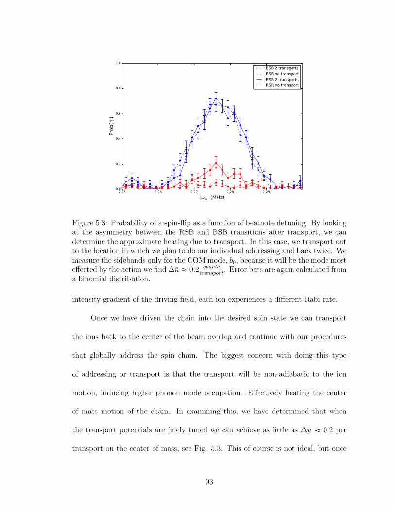
2.25 2.26 2.27 2.28 2.29
|ω∆| (MHz)
0.0
0.2
0.4
0.6
0.8
1.0
Pro
b(↑
)
BSB 2 transports
BSB no transport
RSR 2 transports
RSR no transport
Figure 5.3: Probability of a spin-flip as a function of beatnote detuning. By lookingat the asymmetry between the RSB and BSB transitions after transport, we candetermine the approximate heating due to transport. In this case, we transport outto the location in which we plan to do our individual addressing and back twice. Wemeasure the sidebands only for the COM mode, b0, because it will be the mode mosteffected by the action we find ∆n ≈ 0.2 quanta
transport. Error bars are again calculated from
a binomial distribution.
intensity gradient of the driving field, each ion experiences a different Rabi rate.
Once we have driven the chain into the desired spin state we can transport
the ions back to the center of the beam overlap and continue with our procedures
that globally address the spin chain. The biggest concern with doing this type
of addressing or transport is that the transport will be non-adiabatic to the ion
motion, inducing higher phonon mode occupation. Effectively heating the center
of mass motion of the chain. In examining this, we have determined that when
the transport potentials are finely tuned we can achieve as little as ∆n ≈ 0.2 per
transport on the center of mass, see Fig. 5.3. This of course is not ideal, but once
93

again it is sufficient for out purposes . With tighter foci of our Raman beams and
extensively optimized transport potentials, I am confident that this heating could
be made negligible.
In principle, this is all we need to flip individual spins, however, the difference
in Rabi rate between different ions is not sufficient to truly initialize them in a
clean manner. Therefore, we couple this technique with composite pulse sequences,
described in the next section, to try and obtain a more pure spin configuration.
5.2.2 Composite pulse sequences
0 π/2 π 2π/3 2π
normalized rotation (rad.)
0.0
0.2
0.4
0.6
0.8
1.0
P(↑
)
Rabi
SK1
N2
Figure 5.4: Probability of population transfer as a function of normalized time forthree different pulse sequences. By using different pulse sequences we can get fullpopulation transfer to the spin-up state with more or less dependence on the rotationangle about the Bloch sphere. This plot shows population transfer for a single pulseas well as two composite pulse sequences.
The goal of a composite pulse sequence is to reduce the error from an imperfect
roation around the Bloch sphere without knowledge of the specific error which has
94

occured, see Fig. 5.4. For example if a single pulse has a small amplitude error
O(ε), by repeating this rotation n times the error is reduced to O(εn) [65]. There
have been a few composite pulse sequences developed to compensate for arbitrary
errors, generally these pulses involve doing multiple rotations around the Bloch
sphere about different axes.
0 5 10 15 200.00.20.40.60.81.0
P(↑
)
Rabi
0 5 10 15 200.00.20.40.60.81.0
P(↑
)
SK1
0 5 10 15 20
normalized rotation (rad.)
0.00.20.40.60.81.0
P(↑
)
N2
Figure 5.5: Probability of a population transfer as a function of normalized rotationsfor three different composite pulse sequences. Each color represents a different ionwhich experiences a different intensity of the beatnote. The upper curve shows Rabiflopping with an intensity gradient. The middle curve shows the SK1 pulse sequenceand the bottom curve depicts the N2 pulse sequence.
From theoretical curves of the spin dynamics, we can see the differences in
population transfer between the various pulse sequences we perform as a function of
π-time, see Fig. 5.5. We compare three different sequences of driving pulses: First,
we directly compare the different rates at which individual ion spins are flipped by
turning on a single pulse. Next, we use a bandpass composite pulse sequence known
95

as SK1, which is less sensitive to intensity fluctuations, effectively flattening the
crests and troughs of the sinusoidal oscillations of the Bloch vector [65]. Finally, we
examine a narrow band pulse sequence, N2, which is extremely sensitive to intensity
[50,66]. This pulse sequence is narrowly peaked around a specific normalized π-time.
In the end we choose which pulse sequence to use based on the number of ions and
day-to-day calibrations. The three ion data used in this thesis was taken, almost
exclusively, with the N2 composite pulse sequence.
0 10 20 30 40 50 60 70 80
time (µs)
0.0
0.2
0.4
0.6
0.8
1.0
Pro
b(↑
)
0 10 20 30 40 50 60 70 803456789
10
PM
T c
hannel
Figure 5.6: The lower curve shows calculated spin-up probabilities by implementinga threshold on the PMT data. The semi-transparent lines show a sin2 fit to thedynamics, these curves are only meant as guides to the eye. The heat map showsthe photon count received by PMT channels on our multi-channel PMT. By usinga single pulse there is still a great deal of overlap between individual ions beingflipped up regardless of pulse time. Error bars are again calculated from a binomialdistribution.
By making use of the intensity gradient in the beatnote that we transport ions
over, we try and find a time where we find only one spin flipped for a given pulse
96

Figure 5.7: Single pulse sequence with normalized rotation angle around the Blochsphere. The phase φ represents the axis about which we are performing the rotation.
sequence. In principle we could achieve this with a single pulse, see Fig 5.6 and 5.7,
by manipulating the intensity gradient as well as the ion spacing. However, we can
get much better temporal separation of spin flips by employing the composite pulse
sequences discussed above.
Figure 5.8: The SK1 pulse sequence with normalized rotation angle. The two addi-tional pulses are done about a axes rotated from the initial rotation axis given bythe angle φ.
By applying the SK1 sequence, see Fig. 5.8, we can eliminate some of the
dependence on intensity, for example if a rotation angle, using a single pulse, would
rotate an ion spin state 80% bright, using the SK1 pulse sequence that same rotation
angle rotates the spin state fully bright, see Fig. 5.9. Similarly if a rotation angle,
using a single pulse, would rotate the ion spin state 20% bright, using the SK1
sequence the ion will remain totally dark. However, this comes at the cost of a
reduced effect of the intensity gradient. By separating ions by larger distances this
pulse sequence is quite effective. When trapping only two ions and manipulating
phonons, this is pulse sequence we use for initialization.
For three ion chains, we do much better using the N2 pulse sequence, see Fig.
5.10, because the N2 sequence is so strongly dependent on intensity, see Fig. 5.11.
97

0 10 20 30 40 50 60 70 80
time (µs)
0.0
0.2
0.4
0.6
0.8
1.0
Pro
b(↑
)
0 10 20 30 40 50 60 70 803456789
10
PM
T c
hannel
Figure 5.9: The SK1 pulse sequence results. It allows us to to get very high fidelityspin flips. The semi-transparent lines show the dynamics of perfect SK1 flopping.However as shown in the heat map there is considerable overlap with adjacent spinflips. These curves are meant as guides to the eye. Error bars are again calculatedfrom a binomial distribution.
Figure 5.10: N2 pulse sequence with normalized rotation angle. The two additionalpulses are done about a axes rotated from the initial rotation axis given by the angleφ.
This means we get the largest separation in time of individual spins flipped for the
same intensity gradient. Unfortunately this means that initialization is now very
sensitive to intensity fluctuations and pointing instabilities of the Raman laser. We
have measured these to be < 1% in approximately 100 ms of measurement time.
However, at long time scales the laser intensity can vary by as much as 20%, which
means we have to calibrate the appropriate time to initialize spins several times a
98

day.
0 10 20 30 40 50 60 70 80
time (µs)
0.0
0.2
0.4
0.6
0.8
1.0
Pro
b(↑
)
0 10 20 30 40 50 60 70 803456789
10
PM
T c
hannel
Figure 5.11: N2 pulse sequence measurement, this gives the best separation of spin-flips. This can be most readily observed in the multi-channel PMT where there isa distinct gap between adjacent ion spin flips. The semi-transparent lines show thedynamics of perfect N2 flopping. These curves are meant as guides to the eye. Errorbars are again calculated from a binomial distribution.
To initialize a specific phonon occupation, we will make use of the conditional
nature of our sideband transition, which will only change the phonon occupation if
there is a corresponding spin to flip. To change the phonon state by one quanta,
we need to have only one spin flipped before we apply a RSB. This requires the
individual ion addressing described above so that we can selectively change the spin
state of a specific ion. We expect to exchange the single spin-flip with one additional
excitation of motion.
99

5.3 Phonon State Initialization and Distillation
0.0 0.5 1.0 1.5 2.0
0.0
0.2
0.4
0.6
0.8
1.0
P(↑)
endcenterend
0.0 0.5 1.0 1.5 2.0
0.0
0.2
0.4
0.6
0.8
1.0
popula
tions
↓ ↓ ↓
1 spin up2 spins up↑ ↑ ↑
0.0 0.5 1.0 1.5 2.0
Normalized Time
0.0
0.2
0.4
0.6
0.8
1.0
phonon n
um
ber n=0
n=1
Figure 5.12: Calculation of the evolution of spin populations and phonon numberwith three ions. If we successfully flip an individual spin then we can drive a RSBon the mode we wish to prepare in order to initialize a single excitation in thatmode. The top curve shows the spin dynamics as we initialize an excitation in modeb2 from chapter 2. The middle curve shows the evolution of the spin manifold. Thebottom curve shows the expected evolution of the phonon excitation.
Once we have flipped a single spin, we can drive a RSB to put a single
phonon excitation in a given normal mode. Driving this term results in the state,
100
c↓,↓,↓ |↓, ↓, ↓〉 |1, 0, 0〉+ (c↑,↓,↓ |↑, ↓, ↓〉+ c↓,↑,↓ |↓, ↑, ↓〉+ c↓,↓,↑ |↓, ↓, ↑〉) |0, 0, 0〉, which has
the highest overlap with |↓, ↓, ↓〉 |1, 0, 0〉, but still has a non-zero overlap with a zero
phonon excitation state, see Fig. 5.12. This is because the manifold of possible spin
flips is not a two state manifold. As we drive the spin, which was initialized up,
back down adding a phonon in the process, we also begin to flip up all the other
combinations of one spin flipped up states by removing the phonon we just added.
This process is identical to how phonons were previously removed from the system
during sideband cooling.
This complication requires us to distill only the component of the state which
has the phonon we are interested in, and trace out all other spin components. To
make sure we can start with a pure Fock state of the normal modes we are interested
in, we perform a RSB such that we maximize overlap with |↓, ↓, ↓〉 |1, 0, 0〉, see Fig.
5.13, and then turn on our 369 nm laser tuned to scatter photons from the spin up
state via the 2P1/2 state. The splitting between the two hyperfine ground states we
are using as spin-up and spin-down is large enough that the spin down states do
not couple to the excited state. The spin-down state will remain unaffected by this
light. If we collect any scattered photons, we re-pump the ion chain and repeat this
procedure until we do not detect any scattered photons. This distills our quantum
state to only that component with all spins down in a probabilistic fashion, where
the probability of success is dependent on the mode we are driving and the ion
we individually addressed. This state distillation has not been used before in this
context and constitutes a new tool for engineering specific Fock states in 171Yb+
trapped ion chains.
101

0 10 20 30 40 50 60 70
time (µs)
0.0
0.2
0.4
0.6
0.8
1.0
Pro
b(↑
)central ion
end ion
end ion
0 10 20 30 40 50 60 70
time (µs)
0.0
0.2
0.4
0.6
0.8
1.0
Pro
b
↓ ↓ ↓1 spin up
2 spins up↑ ↑ ↑
Figure 5.13: Measured evolution of the three ion populations. By driving a RSBtransition, we flip a single spin as expected but which ion flips begins to becomeunclear after one exchange of motion with spin. The solid lines on the lower plot aresin2 fits to the data. Error bars are again calculated from a binomial distribution.
To verify that we still maintain purity in our phonon state after this distillation,
we test the coherence of spin motion coupling by Rabi flopping on a RSB of the
mode containing the excitation we introduced. If we have truly distilled |↓, ↓, ↓〉 |1〉
102

0 1 2 3 4 5 6
0.0
0.2
0.4
0.6
0.8
1.0
P(↑)
endcenterend
0 1 2 3 4 5 6
0.0
0.2
0.4
0.6
0.8
1.0
popula
tions
↓ ↓ ↓
1 spin up2 spins up↑ ↑ ↑
0 1 2 3 4 5 6
Normalized Time
0.0
0.2
0.4
0.6
0.8
1.0
phonon n
um
ber n=0
n=1
Figure 5.14: Calculated spin population and phonon number evolution. By drivinga RSB after distillation, hopefully we exchange the single excitation of motion witha single spin flip. These theoretical curves show this for the b0 mode. The top curveshows the spin dynamics of each ion. The middle curve shows the spin-manifoldpopulations. The bottom curve shows the expected evolution of the excitation ofmotion. The time here is normalized to the coupling strength, for these simulationsall of these coupling rates were set to unity.
in whatever mode we want to distill, then we should maintain coherent flopping
between the |↓, ↓, ↓〉 state and the one spin flipped manifold. Any leakage into higher
phonon population or thermal state contamination should manifest as multiple spins
103

being flipped simultaneously. These populations remain negligible, and we take this
to mean our procedure up to this point, including transport and state distillation,
is not overly contaminated with undesirable phonon occupation. We can perform
these experiments on all three modes after multiple steps of distillation.
We look specifically at the case where we are trying to initialize the state
|↓, ↓, ↓〉 |1, 0, 0〉, where the basis for the motion is |b0, b1, b2〉 from before. In this
case, we should expect to see all spins flip equally but not simultaneously as we drive
spin-motion coupling through a RSB on mode b0, see Fig. 5.14. Our results show
that we maintain coherent flopping between the equal spin manifolds5 we expect to
be moving population between, see Fig. 5.15. However, the contrast of both of these
curves is lower than expected. We believe this has to do with imperfect spin-flips in
our individual addressing procedure. If we leave population in the spin-down state
of the ion we are trying to individually address, it will not participate in the phonon
initialization. This specific error is not caught by the distillation procedure.
In the case of the b2 mode, we should expect to see the middle spin flip twice
as much as the outer ions, see Fig. 5.16, given the relative normal mode amplitudes.
Once again we expect that none of the spins should flip simultaneously because
we only have one excitation to exchange. Similar to mode b0, we see a decrease
of approximately 20% in contrast, see Fig. 5.17. This consistency between two
very different modes reinforces our belief that the contrast degradation is due to a
problem in spin initialization before adding a phonon.
5All spins down, one spin up, two spins up, or three spins up.
104

0 50 100 150 200 250 300
time (µs)
0.0
0.2
0.4
0.6
0.8
1.0
Pro
b(↑
)central ion
end ion
end ion
0 50 100 150 200 250 300
time (µs)
0.0
0.2
0.4
0.6
0.8
1.0
Pro
b
↓ ↓ ↓1 spin up
2 spins up↑ ↑ ↑
Figure 5.15: Experimental results of the simulated experiments in Fig. 5.14. Thetop plot shows the measured spin dynamics of each ion. The bottom plot shows thepopulations of the spin-manifolds. Note the reduced contrast in the spin manifoldplot, we attribute this to poor initialization of spin. The solid lines are sine squaredfits to the data of the form A sin2(ωt + φ) + C. Where A, ω, φ, and C are allfit parameters. Error bars are again calculated from a binomial distribution. Theaverage reduced χ2 for the fits on the upper plot is 0.95, for the lower plot theaverage reduced χ2 is 0.985.
105

0 1 2 3 4 5 6
0.0
0.2
0.4
0.6
0.8
1.0
P(↑)
endcenterend
0 1 2 3 4 5 6
0.0
0.2
0.4
0.6
0.8
1.0
popula
tions
↓ ↓ ↓
1 spin up2 spins up↑ ↑ ↑
0 1 2 3 4 5 6
Normalized Time
0.0
0.2
0.4
0.6
0.8
1.0
phonon n
um
ber n=0
n=1
Figure 5.16: Calculated spin population and phonon number evolution. By drivinga RSB after distillation hopefully we exchange the single excitation of motion witha single spin flip. These theoretical curves show this for the b2 mode. The top curveshows the spin dynamics of each ion. The middle curve shows the spin-manifoldpopulations. The bottom curve shows the expected evolution of the excitation ofmotion. Once again the normalized time is set but making the coupling strengthunity and directly integrating the Schrodinger equation.
106

0 50 100 150 200 250 300
time (µs)
0.0
0.2
0.4
0.6
0.8
1.0
Pro
b(↑
)
central ion
end ion
end ion
0 50 100 150 200 250 300
time (µs)
0.0
0.2
0.4
0.6
0.8
1.0
Pro
b
↓ ↓ ↓1 spin up
2 spins up↑ ↑ ↑
Figure 5.17: Experimental results of the simulation shown in Fig. 5.16. As beforethe top plot shows the measured spin dynamics of each ion and the bottom plotshows the populations of the spin-manifolds. The solid lines are sin squared fitsto the data of the form A sin2(ωt + φ) + C. Where A, ω, φ, and C are all fitparameters. The average reduced χ2 for the fits on the upper plot is 0.74, for thelower plot the average reduced χ2 is 0.714. Error bars are again calculated from abinomial distribution.
107

5.4 Readout
In principle, the phonon occupation can be read out by comparing Rabi rates
on the sideband transitions to known phonon occupations. However, this measure-
ment would be subject to calibration errors which would make it less reliable than
we would like it to be. Instead, we will read out the phonon occupation through
a STIRAP process on the red sideband. The effect of this STIRAP procedure is
to move all Fock population from |n〉 → |n− 1〉, and in so doing flip a spin. By
using this STIRAP procedure we are able to do this for wide a range of Fock states
even though they each have Rabi rates that scale like√n. The pulse we use for our
experiment is chirped in both frequency and amplitude [67].
Once mapped to the excited state, we do a spin flip transition to map all of the
excited state populations to the ground state. However, the population associated
with zero excitation, the ground state of the mode, will not have undergone a tran-
sition under the STIRAP process. The subsequent spin flip will put this population
in the spin up state as opposed to the spin down state. If we try and detect the
excited state, and collect any scattered photons we can say our population was in
the |n = 0〉 phonon Fock state at the beginning of this procedure. By repeating
successive iterations of this process, leaving detection for the last step, then we can
measure whether we have population in a given Fock state, see Fig. 5.19. This
technique was proposed recently in the context of Boson sampling with ions [52],
and has been demonstrated extensively for single ion states [49, 67]. We are cur-
rently working on generalizing a similar method for multi-ion chains, however, this
108
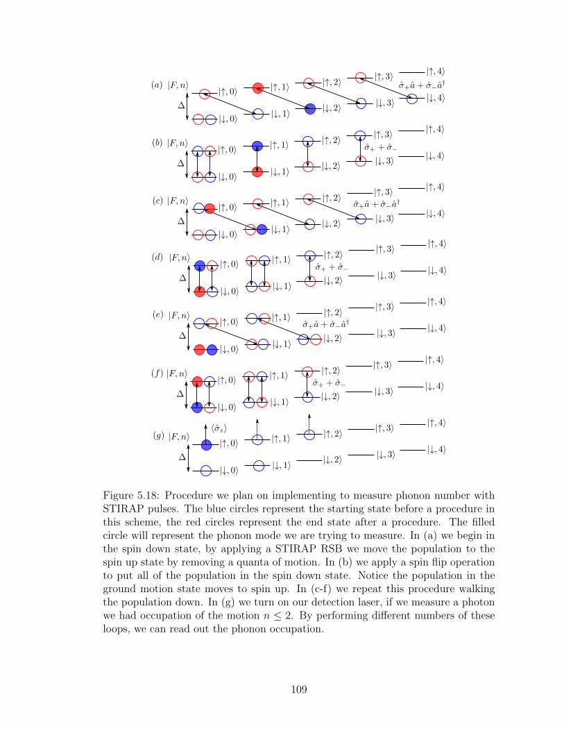
Figure 5.18: Procedure we plan on implementing to measure phonon number withSTIRAP pulses. The blue circles represent the starting state before a procedure inthis scheme, the red circles represent the end state after a procedure. The filledcircle will represent the phonon mode we are trying to measure. In (a) we begin inthe spin down state, by applying a STIRAP RSB we move the population to thespin up state by removing a quanta of motion. In (b) we apply a spin flip operationto put all of the population in the spin down state. Notice the population in theground motion state moves to spin up. In (c-f) we repeat this procedure walkingthe population down. In (g) we turn on our detection laser, if we measure a photonwe had occupation of the motion n ≤ 2. By performing different numbers of theseloops, we can read out the phonon occupation.
109

is complicated by the larger spin manifold. In principle, we can map normal mode
excitations on single ion excitations6 and read out in this way.
6Discussed in depth in section 6.2
110

Chapter 6: Phonon Interference
We have yet to talk about how these modes can be used for anything besides
poor quantum memories. The tricky part is to engineer interactions between normal
modes which will have dynamics that are not well captured by the spin degrees of
freedom of the ion chain. For this we look to the photonics community, where pho-
tons play an identical role to the phonons in our current experiments. In photonics,
interesting physics is achieved by using a network of beam splitters and utilizing
bosonic statistics to generate non-trivial states. It would be ideal to demonstrate
an experiment that has a direct analog to photonics using phonon excitations. This
would also show the versatility of the tools we have been developing thus far. The
demonstration experiment we have chosen to try is to look for Hong-Ou-Mandel
(HOM) interference between phonon modes. I want to take some time to walk
through these experiments, and then give our current results.
6.1 Hong-Ou-Mandel Photon Example
Hong-Ou-Mandel interference is a canonical example of the quantum behavior
of light [68]. The experiment is relatively simple, given a beam splitter with perfect
50/50 visibility, take two identical single-photon sources and impinge those sources
111

Figure 6.1: If a photon from input mode a and an identical photon from input modeb hit the beam splitter at exactly the same time then one measures the coincidenceof both output detectors measuring a photon, the result will be zero due to bosonicstatistics.
on two of the ports of the beam splitter. On the output ports, place two-single
photon detectors. If you vary the amount of time it takes for one of the photons to
hit the beam splitter, there will be a specific time at which point there will no longer
be coincident counts on the detectors, see Fig. 6.1. This is known as the Hong-Ou-
Mandel dip, and it is a consequence of the interference of the photon wavepackets
at the beam splitter1. One way to view this experiment is to consider the beam
splitter as a unitary rotation of input modes to output modes,
1If this dip exceeds 50% this effect exceeds the interference one might expect of classical corre-lations.
112

a† =c† + d†√
2(6.1)
b† =c† − d†√
2(6.2)
Because these operators are bosonoic they commute with each other, specif-
ically [c†, d†] = 0. Then if we consider the input state acting on the vacuum to
generate the two input photons, we end up with input and output states given by,
a†b† |0a, 0b〉 →1
2(c†2 + d†c† − c†d† − d†2) |0c, 0d〉
a†b† |0a, 0b〉 →1
2(c†2 − d†2) |0c, 0d〉
|1a, 1b〉 →|2c, 0d〉 − |0c, 2d〉√
2(6.3)
In other words, when measuring the output, there will be no coincident detec-
tion at different output ports. Just to highlight the point, if the particles interfering
on the beam splitter were fermions, which anti-commute c†, d† = 0, then the
cross terms would not cancel. In fact they would be the only terms due to the
Pauli exclusion principle, and there would only be coincident counts on the de-
tectors. The resulting output state is an entangled state of the two modes. This
basic interference is one way linear optical quantum information processors generate
entanglement [69]. It is also a perfect test for the bosonic nature of our phonons.
Good Hong-Ou-Mandel contrast is indicative of good bosonic statistics; furthermore
113

it requires us to generate specific Fock states and be able to read them out.
To give a more general mathematical description of this phenomena [70], we
can start with two photons which have a joint Gaussian pulse shape β impinging
on a beam splitter with unknown transmission (T ) and reflection (R) coefficients.
The creation and annihilation operators for the input state can be described as an
integral over the pulse time, with corresponding creation operators acting on the
vacuum state,
|11, 12〉 =
∫dt
∫dt′β(t, t′)a†1(t)a†2(t′) |0〉 (6.4)
Where β is given by the overlap of the spectral amplitudes, ζ, normalized in
the following way,
β(t, t′) = ζ(t)ζ(t′) (6.5)
ζ(t) =
(2∆2
π
) 14
e−iω0te−∆2(t0−t)2
(6.6)
1 =
∫dt
∫dt′|β(t, t′)|2 (6.7)
1 = |R|2 + |T |2 (6.8)
The ∆ in the above expression is the spectral bandwidth of the light. In terms
of the output operators, the input operators are defined as,
114

a†1(t) = Ra†3(t) + T a†4(t) (6.9)
a†2(t) = T a†3(t) +Ra†4(t) (6.10)
We can write the integration above in terms of the output operators to obtain,
|11, 12〉 =
∫dt
∫dt′
1
2RT [β(t, t′) + β(t′, t)]
[a†3(t)a†3(t′) + a†4(t)a†4(t′)
](6.11)
+[R2β(t, t′) + T 2β(t′, t)
] [a†3(t)a†4(t′) + a†4(t)a†3(t′)
]|0〉
From the form of the operators, we can conclude that there will be two cases
that will be interesting: The case where we get coincident detection on the output
ports, 〈13, 14|, and those in which we do not, 〈23, 04| and 〈03, 24|. The probability
of the first case is given by,
115

〈13, 14|11, 12〉 =
∫dt
∫dt′[R2β(t, t′) + T 2β(t′, t)
](6.12)[
〈13, 14| a†3(t)a†4(t′) |0〉+ 〈13, 14| a†4(t)a†3(t′) |0〉]
=
∫dt
∫dt′R2β(t, t′) + T 2β(t′, t) (6.13)
P (13, 14) = | 〈13, 14|11, 12〉 |2 (6.14)
= |∫dt
∫dt′R2β(t, t′) + T 2β(t′, t)|2 (6.15)
= R4
∫dt
∫dt′β∗(t, t′)β(t, t′) + T 4
∫dt
∫dt′β∗(t′, t)β(t′, t) (6.16)
+ |R|2|T |2∫dt
∫dt′ [β∗(t, t′)β(t′, t) + β∗(t′, t)β(t, t′)]
= |R|4 + |T |4 + 2|R|2|T |2|J |2 (6.17)
|J |2 =
∫dt
∫dt′β∗(t, t′)β(t′, t) (6.18)
By completing the square and using the normalization convention defined
above we get a term that looks like,
P (13, 14) = 1− 2|R|2|T |2(1 + |J |2) (6.19)
Similarly we can look at the probability that both photons exit the same port
of the beam splitter,
116

〈24, 04|11, 12〉 = 〈04, 24|11, 12〉 =
∫dt
∫dt′√
2
2RT [β(t, t′) + β(t′, t)] (6.20)
P (23, 04) = P (03, 24) = | 〈23, 04|11, 12〉 |2 = | 〈03, 24|11, 12〉 |2 (6.21)
=2
4|R|2|T |2
∫dt
∫dt′| [β(t, t′) + β(t′, t)] |2 (6.22)
= |R|2|T |2(1 + |J |2
)(6.23)
For the special case of a 50/50 beamsplitter, where |R|2 = |T |2 = 12, the
probabilities for each case reduces to,
P (23, 04) = P (03, 24) =1
4
(1 + |J |2
)(6.24)
P (13, 14) =1
2(1− |J |2) (6.25)
We can see that |J |2 is the overlap integral of the photon wavepackets in time.
For the case in which both of these photons have perfect overlap in arrival time and
have the same center frequency, ω0, we say the photons are identical and the overlap
integral |J |2 = 1. For this case, the probability for both photons to exit the same
port is P (23, 04) = P (03, 24) = 12
and the probability that they exit different ports
vanishes, P (13, 14) = 0. This gives rise to the aforementioned Hong-Ou-Mandel dip
in coincident counts as the photon arrival time of one of the wavepackets is scanned.
117

6.2 Hong-Ou-Mandel Phonon Example
For the phonons we create, it can be challenging to create a direct analog of
this beam splitter interaction. Essentially, this requires generating an xi ·xj coupling
of the modes we want to mix. This type of non-linearity requires us to introduce a
gradient between normal modes. That can be difficult without perturbing the ions
motion in such a way as to ruin the Fock states we have prepared. There are three
approaches worth mentioning.
The first approach studied experimentally, but not in this context, involves
driving a gradient of field electric field at the difference frequency between two
modes [71–74]. This gradient needs to spatially overlap with both modes of interest,
and the gradient itself will determine the strength of the coupling. This has been
shown in a micro-fabricated trap where mixing was driven between the in and out of
plane normal modes. There are a few reasons why we find this approach unappealing
for our experiments. First, it is sometimes challenging to drive the nominally DC
potentials without inducing micro-motion and subsequent heating of the normal
modes.
More problematic is the fact that even though the trap electrodes are small,
on the order of 60 µm and they are close ≈ 90µm away from ions, the ions in a chain
are spaced by ≈ 5µm. This means that there needs to be a strong field gradient
between ions created from electrodes that are an order of magnitude farther away.
In practice this means that extremely large voltages must be applied to electrodes to
get any non-negligible coupling. Because our trap has delicate features, for example
118

the trench capacitors used to eliminate RF pick-up on the DC electrodes, we are
limited to no more than 10 V on the DC electrodes. In simulations we estimated this
would allow us to get less than a 10 Hz coupling between different normal modes an
the same trapping axis. One could do better by coupling in and out of plane modes,
however, we would then have to cool twice as many modes which might increase the
length of experiments such that heating effects would start to set in before we could
see any interference.
The second and more promising technique involves weakening the axial trap
depth, which is equivalent to weakening the springs between ions by increasing their
distance from one another [75]. If the distance is made large enough and a single
ion is addressed2 then the addressed mode is more of a local mode than a collective
mode [51]. This local excitation will naturally begin to mix with the other local
modes, and this mixing can be used as a beam splitter between local phonons when
viewed at certain times. As a classical analog, think of beads connected axially
by springs. When the springs are strong and a bead is displaced in the transverse
direction and all the beads participate in the resulting harmonic motion, this is
exciting a normal mode of motion. However, if the springs between beads are
incredibly weak, then a bead displaced will oscillate at its center of mass frequency
before the excitation slowly couples to the other beads. An alternative interpretation
is to consider the fact that the normal modes of motion are the eigenstates of the
confining Hamiltonian, while the local modes are superpositions of the normal modes
and since they are not eigenstates the local modes, they will undergo time evolution
2This is much more easily accomplished now that the ions are separated by much larger distances
119

into one another at a rate given by the difference in their associated energies. The
hopping between the local modes can be thought of as a beam splitter between local
modes. This hopping between local modes goes like,
ti,i+1 ∝ω2z
2ωx,y(6.26)
This coupling has been shown to exhibit HOM type interference using two
trapped Ca+ ions in a macro-fabricated trap [75]. The main issue with this type of
coupling is that it is very difficult to engineer the coupling exactly. It is difficult to
modify the DC potential without inducing heating, in the experiments where this
was demonstrated the potential was not changed and they observed the phonons
hop back and forth. But if you want to stop the hopping for readout or to freeze
the state in a given phonon configuration, this can be challenging to do with DC
electrodes.
The way in which we are trying to induce this coupling relies on our Raman
interaction. In Chapter four, we wrote down the coupling, for an arbitrary length
ion chain, of the ion chain motion to light. Before making the Lamb-Dicke approx-
imation that Hamiltonian took the form,
HI =∑j
Ωσ+j e
iωHF t∏i
e[iηi,j(a†i eiωit+aie
−iωit)]e−iω∆t + h.c. (6.27)
By saying that the parameter η was small, we expanded the exponential in
a Taylor series. However, not only are the terms in the expansion separated in
120

strength by η, they are also spectrally resolved by combination of the normal mode
frequencies. Therefore there are terms that are higher order in η which separate
spectrally and can be driven [76]. More concretely, there exists a term that is
second order in η that has the form,
O(η2)→ HRWAI =
∑j
ηi,jηk,jΩ(σ+j aia
†k + σ−j a
†i ak)
Once an appropriate rotating wave approximation is made, requiring the driving
field to be at the difference frequency of the two modes of interest ω∆ = ±|ωi−ωk|.
This term looks a lot like the traditional beam splitter Hamiltonian,
HBS ∝ (aia†k + a†i ak) (6.28)
If we can drive two colors, one color at the positive difference frequency, and
one at the negative difference frequency then we can drive a Hamiltonian which is
identical to this beam splitter Hamiltonian for the phonon modes, see Fig. 6.3
HHOM =∑j
ηi,jηk,jΩ(σ+j + σ−j )(aia
†k + a†i ak) (6.29)
This is the term we are attempting to drive when we induce our HOM coupling.
The reason we find this coupling scheme appealing is that in principle we can drive
many different interference terms by adding additional frequencies to our Raman
beatnote, which is relatively trivial. It is also an externally driven interaction, which
allows us to turn on and off the coupling at will. This would in principal allow us
121

0.0 0.1 0.2 0.3 0.4 0.5 0.60.0
0.2
0.4
0.6
0.8
1.0
P(↑)
end ioncentral ionend ion
0.0 0.1 0.2 0.3 0.4 0.5 0.6Normalized Time
0.0
0.2
0.4
0.6
0.8
1.0
popula
tions
↓ ↓ ↓
1 spin up2 spins up↑ ↑ ↑
Figure 6.2: Theory plots describing the evolution, under the Hamiltonian HHOM =∑j ηi,jηk,jΩ(σ+
j +σ−j )(aia†k+ a†i ak), of the quantum state as a function of drive time.
The upper plot shows how the individual spins should flip in a three ion chain. Thebottom plot dipicts the evolution of the spin manifolds. The normalized time is aresult of setting ηi,jηk,jΩ = 1 when calculating the state evolution.
to tune the visibility of the beam splitters we are creating. Finally, this type of
interaction only relies on the normal modes; we are not required to modify the DC
potential, and incur the heating that might result. Finally, once the interaction is
turned off the modes will stop evolving which makes measurement less daunting.
6.2.1 Results
We have attempted to drive the interference term detailed above, and although
our results thus far are not in agreement with theory, they give us some hope for a
way forward and hint at what are our current limitations. Using the tools developed
122

0.0 0.1 0.2 0.3 0.4 0.5 0.6Normalized Time
0.0
0.2
0.4
0.6
0.8
1.0
popula
tions
N=0N=1N=2
Figure 6.3: Theory plots describing the evolution of the quantum state as a functionof drive time. This plot shows the evolution of the motion state for one of the modesas function of drive time. Where the red curve is the evolution of the |n = 2〉 phononstate, green show the|n = 1〉 phonon state, and blue is the |n = 0〉 phonon state.In the beginning we initialize in |n = 1〉 and this state oscillates between this and|n = 0〉 + |n = 2〉, very similar to a Hong-Ou-Mandel experiment. The normalizedtime is a result of setting ηi,jηk,jΩ = 1 when calculating the state evolution.
in the previous chapters, we have tried to initialize our chain of three ions in the
state,
|Ψ〉 = |ψ〉spin |ϕ〉motion (6.30)
= |↓, ↓, ↓〉 |1, 0, 1〉 (6.31)
When we drive the HOM term, we are going to look at the spin component of
123

the three ion state, see Fig. 6.2. By using spin as a witness, we should expect to
see flopping between the all spin down state ψ0 = |↓, ↓, ↓〉 and the one spin flipped
up manifold ψ = |↑, ↓, ↓〉 + |↓, ↑, ↓〉 + |↓, ↓, ↑〉, without any two spins being flipped
simultaneously. This condition comes from the coupling we are trying to drive,
which can only exchange one beam splitter excitation with one spin flip excitation.
If we start with φ0 = |1, 0, 1〉, then the only other coupled state of the phonons is
φ = |2, 0, 0〉 − |0, 0, 2〉.
What we observe is that we can induce some mixing, however the coherence
of this mixing appears to be limited, see Fig. 6.4. What is interesting is that the
decoherence we observe is still confined to the spin manifold we expect to couple
to, which is not what we would expect if heating were the limiting factor. In
fact, if the purity of the phonon state was limiting us, we would expect that the
other spin manifolds, two spins and all spins being flipped up, would play a role
in the dynamics. Our ability to create the φ0 = |1, 0, 1〉 Fock states of motion is
all that limits how many spins are flipped. Our current working theory as to why
the coherence is limited in this manner has to do with the stability of transverse
mode frequencies. In Chapter 2, we showed that the transverse mode frequency
is proportional to the RF voltage, ωx,y ∝ VRF and as discussed previously in this
chapter, the HOM terms we are driving are of order η2. For fixed interaction time
this means that these terms are a factor of η more narrow than a RSB or BSB. To
maintain coherence the transverse secular frequencies must be stable to better than
a fraction of the linewidth of those transitions. This means that the VRF must be
stable to much less than the linewidth of the HOM term. We estimate this level of
124

200 300 400 500 600 700 800 900 1000
time (µs)
0.0
0.2
0.4
0.6
0.8
1.0
Prob(↑
)central ionend ionend ion
200 300 400 500 600 700 800 900 1000
time (µs)
0.0
0.2
0.4
0.6
0.8
1.0
Prob
↓ ↓ ↓
1 spin up2 spins up↑ ↑ ↑
Figure 6.4: The state is initialized to ψ0 = |↓, ↓, ↓〉 |1, 0, 1〉. By driving the HOMterm, we see qualitatively what we expect, namely only the one spin flipped manifoldis participating in the interaction. The solid lines on the lower curves are sin2 fits tothe data of the form A sin2(ωt+φ)+C. Where A, ω, φ, and C are all fit parameters.The average reduced χ2 for the fits on the upper plot is 0.887, for the lower plotthe average reduced χ2 is 0.785. Error bars are again calculated from a binomialdistribution.
stability as,
125

V0 = ωx,y (6.32)
δω <γ
10(6.33)
δω =ωx,yV0
δV (6.34)
δV <γ
10ωx,yV0 (6.35)
Where the term γ is the linewidth of the RSB or BSB, experimentally these
transitions are 50 kHz wide with a center frequency of 2.7 MHz, which means the
HOM term should be approximately 5 kHz wide. This means that the voltage must
be stable to a part in 104 for us to be able to drive coherent flopping:
δV
V0
<γ
10ωx,y(6.36)
<5kHz
10 · 2.7MHz(6.37)
< 2 · 10−4 (6.38)
From the data we have taken for the HOM drive so far we have much more like
a part in 103 stability. To verify this, we took overlapping Allan deviation (OVAD)
measurements of the frequency of the BSB transition [43]. We accomplish this by
doing Ramsey spectroscopy. We applied a π/2 pulse on a cold BSB and wait a time
τ and apply another π/2 pulse. By varying the delay τ , we obtained a fringe which
126

we can fit to determine the frequency of the BSB. For our purpose, it is important
to make the time τ ≥ 200 µ s as this is the relevant time for our fastest HOM drive
time. By repeating this measurement as fast as we can over an hour or more, we
were able to calculate overlapping Allan deviations for the carrier as well as the
BSB. The overlapping Allan deviation is given by [77],
σ2y =
1
2m2(M − 2m+ 1)
M−2m+1∑j=1
j+m−1∑i=j
[yi+m − yi]
2
(6.39)
100 101 102 103
Tau (s)
10-2
10-1
100
101
102
103
Overl
appin
g A
llan d
evia
tion (
Hz)
BSB Mode 1
BSB Mode 2
Carrier
White f Noise
Random Walk f Noise
Figure 6.5: Allan deviation of the frequency of the b0 and b1 modes via Ramseyspectroscopy, we can see that the drifts in the sidebands are a limiting factor inperforming the desired HOM interaction.
When compared to the carrier the BSB has substantially worse stability, which
means the dominate drift is not the beatnote itself, see Fig. 6.5. We see that at
127

the earliest time scales we can measure the BSB is already drifting with a slope
similar to a random frequency walk. This implies that over a few seconds the BSB
has moved by 100 Hz, because the distillation is probabilistic these experiments can
take minutes from the first scan point to the last scan point. If the sidebands are
moving by a part in 103 during this time, as the last few points in the plot suggest,
this accounts for at least a portion of our loss of contrast.
100 101 102 103
Tau (s)
100
101
102
Overl
appin
g A
llan d
evia
tion
Amplitude
100 101 102 103
Tau (s)
101
102
103 Frequency
Figure 6.6: Allan deviation after better stabilization. The blue points are the sameas the points in Fig. 6.5, the pink and purple points represent recent improvements inthe stabilization of the mode frequencies. Where we have also measured the stabilityof the amplitude of Ramsey fringe we measure, this gives us an indication of theintensity drift of the beatnote. This is on the same order as the best stabilizationachieved for similar stabilization circuits, and we still believe this may be the limitingfactor in driving interference.
We think this is by far the limiting factor in driving our HOM terms. Recently,
we have been trying to improve on the stabilization of this frequency by better
128

stabilization the RF drive frequency. In doing so, we have made some improvements
on the above results, see Fig. 6.6. Specifically we have temperature stabilized the
helical resonator as well at the rectifier we use. We also have integrated a part per
million stable voltage reference into the locking circuitry, this is done to stabilize
the setpoint of the servo controller. However, we still believe this to be our limiting
factor. This in fact is what motivated us to try and the develop phonon excitation
readout discussed in section 5.4. This would allow us to look at the external degree
of freedom as well as the spin degree of freedom.
129

Chapter 7: Outlook
7.1 Future Improvements
The intent of this chapter is to discuss some of our strategies for mitigating
the problems we have encountered so far and try to motivate why these tool could
be interesting in the future. We need to find a way to increase the coherence of the
HOM interference we have seen thus far. We have begun by temperature stabilizing
all the components in the RF stabilization circuit as well as try and find what
component in that circuit 1 is inducing the most noise.
The biggest hurdle will be any out of loop noisy reactive elements in the
vacuum chamber itself. In principle, if the RF leads are moving in the chamber this
could change the line inductance and lead to a shift between measured tap voltage
and trap voltage. This shift only has to be a part in 103 before it would account for
all of the drifts we see in the experiment. If there is noise in the RF voltage picked
up after the resonator, the feedback to the resonator itself will be limited in the
bandwidth to the linewidth of the resonator. With feedback before the resonator,
precisely because the helical resonator is a very good filter, it will be difficult to
address frequencies that couple onto the RF line after the resonator.
1Discussed fully in Chapter 3.3.2.2.
130

There are two approaches we have devised to address these issues. We can
move away from using transverse modes and instead couple to the axial modes of
motion. This has two advantages, as stated in Chapter 2: First, the axial modes
depend on the DC trapping voltages, which are much easier to stabilize and can
be heavily low-pass filtered. Secondly, all of the mixing terms will have similar
difference frequencies, which may make future experiments less challenging. The
biggest problem with the axial modes is that they are at lower frequencies. Because
the heating rate as well as the Doppler limit depend on this frequency, it can be
much harder to cool these modes. Despite these drawbacks, with the voltages we
are currently applying, we think we should be able to achieve axial frequencies of
approximately 1 MHz.
The most invasive change, which would require us to break vacuum and replace
the trap with a different trapping architecture, would be to arrange true individual
addressing. The way in which we would achieve this is by making use of a new
trap design, the HOA trap, where the NA from the side of the trap is around 0.25.
This trap also has a slot through the trapping structure which allows tightly focused
beams to be sent through the trap. This change is planned to occur in the next
year, and this will require most of the experiment be dismantled for a few months.
Luckily, the infrastructure of optics and electronics can readily be re-aligned to the
new chamber assembly when it is under vacuum.
In conclusion, we have demonstrated a toolset for initializing and reading out
the external degrees of freedom in a trapped ion chain. We do this with the hope of
being able to utilize this additional quantum resource in experiments that require
131

sampling from bosonic distributions2. This experiment is of interest because it is
classically very difficult, P#-complete, to determine the probability of a specific
output configuration from a bosonic distribution of output configurations derived
from a network of linear beam splitters [54, 78]. If an experiment can bound that
probability for a sufficiently large number of output modes, even to a multiplicative
factor, it would be interesting to several communities of scientists [56].
2See Appendix B for more details on Boson Sampling.
132

Appendix A: Laser locking
Locking the frequency of our laser sources is of paramount importance to
performing high fidelity operations. In previous chapters, there was a discussion of
how we lock the frequency of the Raman beatnote, but the locks used to stabilize
the frequencies of our various CW laser sources was left for this appendix. The
reason why this is so challenging is two-fold. Firstly, we are trying to lock a wide
spectral range of wavelengths from 369 nm to 935 nm1. Secondly, the 369 nm light is
far enough into the blue that certain traditional locking schemes can prove difficult.
This appendix is intended to discuss the several ways we have attempted to lock
our lasers, as well as the planned improvements to our laser locking scheme.
A.1 Wavemeter Locking
The current, unsustainable, locking scheme we are using involves a waveme-
ter from High Finesse, this instrument has an accuracy of 50 MHz around the 369
nm wavelength, a precision of approximately 5 MHz, and returns a measurement
of wavelength approximately every 2 seconds. These wavemeters operate by cou-
pling light to a series of Fizeau interferometers of different lengths. By comparing
1Where some experiments in our group have Ba+ wavelengths peppered throughout that region.
133

the interference pattern from each of these interferometers, software calculates the
wavelength based on an interference pattern of a known calibration wavelength.
The operational implementation of this lock is trivial, the wavemeter, a commercial
product, determines the wavelength of the light you send to it via an optical fiber.
One can then use that reading to feedback to the frequency of an ECDL by adjust-
ing the cavity length or the diode current. The main issues with this type of lock
involves timing, and for our purposes precision.
In the ion trapping community, as long as you can trap one ion then you can
always use the ion as an accurate reference in this case the wavemeter. Therefore, we
do not necessarily need high accuracy, just high precision. The problem, arises when
you want to lock multiple wavelengths with this method using only one wavemeter.
The cited precision specifications are only valid within a 2 nm band around the
calibration wavelength. More problematic is how to couple all of these wavelengths
into the same device. Until recently, there was only one port into these wavemeters,
which meant a switch needed to be used. The switches generally sold for these
devices work by taking many input fibers and directing them sequentially onto an
output coupler using a MEMS mirror.
There are two problems with this. First, to be broadband the switch uses mul-
timode optical fiber. By sending multimode light into the wavemeter, the precision
specification will be degraded up to two orders of magnitude. The second problem
is that the time it takes to switch between wavelengths can dramatically impact the
bandwidth of a feedback loop that is relying on a measurement from the wavemeter.
134

A.2 Locking via discharge cells
Figure A.1: The optics path for using a hollow cathode lamp in a polarizationspectroscopy configuration. This requires interrogation of the 174Yb+ isotope. Toshift the 174Yb+ line onto the 171Yb+ S1/2 → P1/2 resonance requires an EOM oranother source of 369 nm light beatnote referenced to 174Yb+. Because the ionsignals in the cell are so small we use lock-in amplification by modulating the powerof the pump light via an AOM to achieve sufficient signal strength.
If for a moment we wish to only lock the 369 nm line and we wish to do
so in a very accurate way, we can think about locking the laser to a cell of Yb+
ions. This is most readily achieved by taking a hollow cathode lamp of Yb and
running a large amount of current through the lamp, 10-30 mA, to create a plasma
of Yb. Once a plasma is achieved, 369 nm light can be locked to the atoms in
whatever way is most convenient. The most commonly used lock for this setup is a
polarization lock [79–81]. This lock works by comparing the differential absorption
of polarized light as the light is swept over resonance. By comparing the amplitude
of transmitted light of different polarizations, a dispersive curve can be obtained
135

with a zero crossing at the peak of resonance. This works because the presence of
the pump changes the proportion of absorbed probe light of different polarizations.
We can see this is we follow a derivation of transmitted intensity [82]. First, we note
that a linearly polarized field in the circular polarization basis is of the form,
E = E0
(cosφ
sinφ
)= E
e−iφ
2
[1
i
]+eiφ
2
[1
−i
](A.1)
After passing through the cell, there will be different absorption of the two
polarizations, where we are ignoring the birefringent effects of the windows. The
probe beam will have an electric field.
E = E0
e−iφ
2
[1
i
]e−L(iω
cn++
α+2
) +eiφ
2
[1
−i
]eL(iω
cn−−
α−2
)
(A.2)
= E0e[−i(ωc nL−iα
L2 )]
e−iφ
2
[1
i
]eiΩ +
eiφ
2
[1
−i
]e−iΩ
(A.3)
Ω =ωL
8c(4∆n− i∆α) (A.4)
Where the ωcn term corresponds to the phase shift the light acquires passing
through the gas. We define ω as the frequency of the light and n as the index of
refraction of the gas. The absorption of the light is defined as α±. The measurement
we want to make is a differential measurement of the two different polarizations in
the linear basis. By using a Wollaston prism to spatially separate both polarization
and then direct each onto one port of a differential photodiode we can make this
differential measurement. In this case, the intensity of the signal we mesure will be,
136

Isig = Iy − Ix (A.5)
= I0e−αL cos
(2φ+
Lω
c∆n
)(A.6)
We can use the Kramers-Kronig dispersion relation to relate ∆α and ∆n, ∆n =
cω0
x1+x2 ∆α, whose parameters we will define shortly. If we make the approximation
that the accumulated polarization angle is small, and we set φ = π4
to maximize our
sensitivity to polarization, we can make a small angle approximation. This leaves
the following equation for the intensity of our signal,
Isig = −I0e−αL
(L∆α0
x
1 + x2
)(A.7)
x =ω0 − ωΓ0/2
(A.8)
From this equation we see that we get a dispersive curve, where there is a zero
crossing on resonance. We can use this curve to feedback to the frequency of our
laser source. The problem here, is that there will be very few 171Yb+ ions and the
signal from these atoms will be small and will also be convoluted with all the other
isotope signals. This leads to a DC offset in the zero crossing of the line we are
interested in locking. In practice, we found it necessary to apply EOM sidebands to
the pump and probe light to align the signals derived from the much more prevalent
174Yb+ isotope with the 171Yb+ resonance we were interested in locking. What we
137

found when using this lock was that sufficient lock performance, < 2 MHz drift of
the laser as measure by the ion, required very specific parameters of the lock and
that small deviations from these parameters could dramatically and adversely affect
lock performance.
A.3 Transfer Cavity Locking
Figure A.2: The optics path for our scanning transfer cavity. The separation ofwavelength can be accomplished with a variety of off the shelf filters. The photodi-odes used depend on the electronics which digitize this signal. Ideally the responsetime of the photodiode is matched to the speed of the ADC to minimize dark counts.
The approach we are pursuing is to lock all of the lasers to a scanning opti-
cal cavity [83]. Light impinging on a Fabry-Perot interferometer will be resonant
when the frequency of light satisfies the resonance condition, ν = m c2nL
where m
138

is a positive integer. By comparing the positions of resonances in a scan of the
cavity length, we can compare frequencies of disparate laser sources. This can be
accomplished while canceling the dependence of the resonance frequencies on the
length of the cavity [84]. If one of these lasers is stabilized elsewhere to a known
reference frequency, then we can use the cavity to stabilize the other laser sources to
this laser. This can be seen if we compare the resonance condition for two adjacent
cavity resonances of the reference laser to a laser we want to stabilize,
Mλref = 2nrefL0 (A.9)
Mλref +λref
2= 2nref (L0 + ∆L0) (A.10)
Nλsig = 2nsigα∆L0 (A.11)
(A.12)
Where ∆L0 corresponds to scanned length of the cavity, which is less than the
total length. The term α∆L0 is a position along that scanned length. The terms
N and M are integers associated with the cavity resonance and nref is the index of
refraction for the reference laser. In more physical terms, these equations represent
the length change of the cavity necessary to see two reference lines, where we have
arranged to have a resonance of the laser we are going to lock in-between these
resonances. From these equations, we can solve for the wavelength of the signal
light as a function of reference light.
139

L0 =Mλref2nref
(A.13)
∆L0 =
(M + 1
2
)λref
2nrefL0
− 1 (A.14)
λsig = λrefnsignref
2M + α
2N(A.15)
Therefore if use the value of α as our set point, in a feedback loop we can
effectively cancel out the length of the cavity, L0, to first order. In practice, we
must also stabilize the static length of the cavity L0 to minimize the effect of pizeo
non-linearities. We do this by stabilizing the value of ∆ between the two reference
resonances. This approach has the advantage that, in principle, we can lock all of
the lasers to a single reference. Moreover, this can be accomplished without a large
amount of overhead 2 in laboratory equipment. This is because the laser frequencies
do not need to be tuned to the resonance as along as the element translating the
mirrors of the cavity has enough throw to cover all the wavelengths.
The obvious problem with this lock is that the feedback bandwidth depends on
the rate at which the scanned mirror can be translated. For larger mirrors, this rate
can be truly limiting. In our current setup we use a 1 inch mirror and can only scan at
a rate of approximately 100 Hz. However, by increasing the overhead involved with
locking these lasers, one can do a Pound-Drever-Hall lock the cavity [85], operated
as a static cavity, with much larger bandwidth.
2By overhead, I am referring to the AOMs, EOMs, and assorted electronics that would beneeded to assure that the lasers are resonate with a static cavity.
140

Appendix B: Boson Sampling
In this section I am going to give a brief view of an experimentalist of how a
Boson sampling experiment would work, and why it is interesting. Boson sampling
is an interesting candidate experiment in the context of building a quantum device
which can perform some simulation of computation that a classical computer can
never hope to achieve. The experiment is as follows, given a set of Fock modes,
we populate some known number state of those modes. If these modes then un-
der go some form of coherent mixing, under a unitary transformation, U , and the
excitation occupation of the output modes is measured, the probability of getting
population out on specific configurations of output channels depends on the matrix
elements of U which mixed input modes to specific output modes. This probability
is proportional to the permanent of a sub-matrix of U which does this mapping of
input modes to output modes [56]. Specifically, this sub-matrix is constructed from
elements of column vectors corresponding to the initial excitation, where the spe-
cific elements of these vectors are chosen corresponding to the rows of the measured
output configuration. More formally, given the input state |ψ〉 the general output
state will be |Γout〉,
141

|Ψ〉 = |ψ1, ψ2, ..., ψM〉 (B.1)
|Γout〉 =∑s
cs
∣∣∣φ(s)1 , φ
(s)2 , ..., φ
(s)M
⟩(B.2)
Where the sum is over all possible configurations of output excitations. The
probability of measuring a specific output configuration is then given by,
Ps(Φs|Ψ) =|Per(U (Φs|Ψ))|2∏Mj=1 φj!
∏Mi=1 ψi!
(B.3)
The reason why this experiment is interesting is that, from the above calcu-
lation we have shown that to calculate the probability of getting a specific output
configuration requires calculating the permanent of a matrix, and in principle, this
matrix can be large. This is significant because calculating the permanent is in-
credibly challenging classically, it belongs to the complexity class P#, and is in fact
P#-complete. P# is not a class of decision problems like NP, instead it is a class
of functions and in a sense can be related to a class of problems associated with
determining the number of solutions to NP problems. Classically the most efficient
algorithm for calculating the permanent of an N × N matrix is of order O(n22n).
This implies that reasonably small systems can become intractable for a classical
computer.
However, the experimental implementation of such an experiment seems fea-
sible. In the linear optics community people are pursuing experiments in this vein
142

for quite some time [56] [86]. Recently there have proposals on how to accomplish
similar experiments with trapped ions [52]. The advantage to ions is that it might
be easier to scale the number of ions, which would increase the number of modes
and complexity of the classical computation. This is compared to scaling up the
number of single photon sources, the bosonic excitations used in photonic boson
sampler. The current state of the art in the photonics community is a 10 photon
boson sampler [86], in the ion trap community no experimental implementations of
boson sampling have been demonstrated.
To be clear, the experimental implementation would not hope to reconstruct
the permanent of the unitary, U . Such an experiment would take exponentially
many measurements and would be highly limited by realistic error models [87, 88].
However, if an experiment can determine the probability of getting a given output
mode configuration to within even some multiplicative factor for a sufficiently large
U ; this might still constitute a demonstration of a quantum device performing a
classically intractable problem. Even if an experiment was to demonstrate such a
calculation the question of how to verify that the output probability was actually
sampled from the unitary of interest is an open question [55]. However, there are
some theoretical proposals and schemes to verify that the sampled distribution was
not uniform [89,90].
143

Bibliography
[1] M. Reiher, N. Wiebe, K.M. Svore, D. Wecker, and M. Troyer. ElucidatingReaction Mechanisms on Quantum Computers. arXiv, 1605(03590):1–28, 2016.
[2] Richard P. Feynman. Simulating physics with computers. International Journalof Theoretical Physics, 21(6-7):467–488, 1982.
[3] D Wineland, C Monroe, W Itano, D Leibfried, B King, and D Meekhof. Ex-perimental issues in coherent quantum-state manipulation of trapped atomicions. Journal of Research of the National Institute of Standards and Technology,103(3), 1998.
[4] Rainer Blatt and David Wineland. Entangled states of trapped atomic ions.Nature, 453(7198):1008–1015, jun 2008.
[5] Thaddeus Ladd, Fedor Jelezko, Raymond Laflamme, Yasunobu Nakamura,Christopher Monroe, and Jeremy O’Brien. Quantum computers. Nature,464(7285):45–53, 2010.
[6] Jacob Smith, Aaron Lee, Philip Richerme, Brian Neyenhuis, Paul W Hess,Philipp Hauke, Markus Heyl, David A. Huse, and Christopher Monroe. Many-body localization in a quantum simulator with programmable random disorder.Nature Physics, 12(10):907–911, jun 2016.
[7] R Blatt and C F Roos. Quantum simulations with trapped ions. Nat. Phys.,8(4):277–284, 2012.
[8] D. Kielpinski, C. Monroe, and D. J. Wineland. Architecture for a large-scaleion-trap quantum computer. Nature, 417(6890):709–711, jun 2002.
[9] Yangchao Shen, Joonsuk Huh, Yao Lu, Junhua Zhang, Kuan Zhang, ShuainingZhang, and Kihwan Kim. Quantum simulation of molecular spectroscopy intrapped-ion device. arXiv, pages 1–17, 2017.
144

[10] H.G. Dehmelt. Radiofrequency Spectroscopy of Stored Ions I: Storage. InAdvances in Atomic and Molecular Physics, pages 53–72. 1968.
[11] Wolfgang Paul. Electromagnetic Traps for Charged and Neutral Particles (No-bel Lecture). Angewandte Chemie International Edition in English, 29(7):739–748, 1990.
[12] D Hucul, I V Inlek, G Vittorini, C Crocker, S Debnath, S M Clark, and C Mon-roe. Modular Entanglement of Atomic Qubits using both Photons and Phonons.ArXiv, 20742(July 2015):1–6, 2014.
[13] S. Debnath, N. M. Linke, C. Figgatt, K. A. Landsman, K. Wright, and C. Mon-roe. Demonstration of a small programmable quantum computer with atomicqubits. Nature, 536(7614):63–66, aug 2016.
[14] J. D. Wong-Campos, K. G. Johnson, B. Neyenhuis, J. Mizrahi, and C. Monroe.High resolution adaptive imaging of a single atom. arXiv, (July):1–9, 2015.
[15] J I Cirac and Peter Zoller. A scalable quantum computer with ions in an arrayof microtraps. Nature, 404(6778):579–81, 2000.
[16] C Monroe and J Kim. Scaling the Ion Trap Quantum Processor. Science,339(6124):1164–1169, mar 2013.
[17] C. J. Ballance, T. P. Harty, N. M. Linke, M. A. Sepiol, and D. M. Lucas. High-Fidelity Quantum Logic Gates Using Trapped-Ion Hyperfine Qubits. PhysicalReview Letters, 117(6):060504, aug 2016.
[18] J. Zhang, P. W. Hess, A. Kyprianidis, P. Becker, A. Lee, J. Smith, G. Pagano,I.-D. Potirniche, A. C. Potter, A. Vishwanath, N. Y. Yao, and C. Monroe.Observation of a discrete time crystal. Nature, 543(7644):217–220, mar 2017.
[19] Fayaz Shaikh, Arkadas Ozakin, Jason M. Amini, Harley Hayden, C. S. Pai,Curtis Volin, Douglas R. Denison, Daniel Faircloth, Alexa W. Harter, andRichart E. Slusher. Monolithic Microfabricated Symmetric Ion Trap for Quan-tum Information Processing. arXiv preprint arXiv: . . . , page 911, may 2011.
[20] Fayaz A. Shaikh and Arkadas Ozakin. Stability analysis of ion motion in asym-metric planar ion traps. Journal of Applied Physics, 112(7):074904, oct 2012.
[21] J. Chiaverini, R. B. Blakestad, J. Britton, J. D. Jost, C. Langer, D. Leibfried,R. Ozeri, and D. J. Wineland. Surface-Electrode Architecture for Ion-TrapQuantum Information Processing. Quantum Information and Computation,5(6):419–439, 2005.
[22] Emily Mount, So-Young Baek, Matthew Blain, Daniel Stick, Daniel Gaultney,Stephen Crain, Rachel Noek, Taehyun Kim, Peter Maunz, and Jungsang Kim.Single qubit manipulation in a microfabricated surface electrode ion trap. NewJournal of Physics, 15(9):093018, sep 2013.
145

[23] J. True Merrill, Curtis Volin, David Landgren, Jason M. Amini, KennethWright, S. Charles Doret, C. S. Pai, Harley Hayden, Tyler Killian, Daniel Fair-cloth, Kenneth R. Brown, Alexa W. Harter, and Richart E. Slusher. Demon-stration of integrated microscale optics in surface-electrode ion traps. NewJournal of Physics, 13, 2011.
[24] Andre Van Rynbach, Peter Maunz, and Jungsang Kim. An integrated mirrorand surface ion trap with a tunable trap location. Applied Physics Letters,109(22):221108, nov 2016.
[25] Erik W. Streed, Benjamin G. Norton, Andreas Jechow, Till J. Weinhold, andDavid Kielpinski. Imaging of Trapped Ions with a Microfabricated Optic forQuantum Information Processing. Physical Review Letters, 106(1):010502, jan2011.
[26] D L Moehring, C Highstrete, D Stick, K M Fortier, R Haltli, C Tigges, andM G Blain. Design, fabrication and experimental demonstration of junctionsurface ion traps. New Journal of Physics, 13:75018.
[27] Kenneth Wright, Jason M. Amini, Daniel L. Faircloth, Curtis Volin, S. CharlesDoret, Harley Hayden, C. S. Pai, David W. Landgren, Douglas Denison, TylerKillian, Richart E. Slusher, and Alexa W. Harter. Reliable transport through amicrofabricated X-junction surface-electrode ion trap. New Journal of Physics,15, 2013.
[28] C. M. Shappert, J. T. Merrill, K. R. Brown, J. M. Amini, C. Volin, S. C. Doret,H. Hayden, C. S. Pai, K. R. Brown, and A. W. Harter. Spatially uniformsingle-qubit gate operations with near-field microwaves and composite pulsecompensation. New Journal of Physics, 15, 2013.
[29] L. Deslauriers, S. Olmschenk, D. Stick, W. K. Hensinger, J. Sterk, and C. Mon-roe. Scaling and Suppression of Anomalous Heating in Ion Traps. PhysicalReview Letters, 97(10):103007, sep 2006.
[30] D F V James. Quantum dynamics of cold trapped ions with application toquantum computation. Applied Physics B: Lasers and Optics, 66(2):20, 1997.
[31] S. Olmschenk, K. C. Younge, D. L. Moehring, D. N. Matsukevich, P. Maunz,and C. Monroe. Manipulation and detection of a trapped Yb+ hyperfine qubit.Physical Review A - Atomic, Molecular, and Optical Physics, 76(5):1–9, 2007.
[32] Ye Wang, Mark Um, Junhua Zhang, Shuoming An, Ming Lyu, Jing Ning Zhang,L. M. Duan, Dahyun Yum, and Kihwan Kim. Single-qubit quantum memoryexceeding $10$-minute coherence time. pages 1–6, jan 2017.
[33] S. Olmschenk, D. Hayes, D. N. Matsukevich, P. Maunz, D. L. Moehring, K. C.Younge, and C. Monroe. Measurement of the lifetime of the 6p 2P1/2 level ofYb+. Physical Review A, 80(2):022502, aug 2009.
146

[34] Chr Balzer, A. Braun, T. Hannemann, Chr Paape, M. Ettler, W. Neuhauser,and Chr Wunderlich. Electrodynamically trapped Yb+ ions for quantum in-formation processing. Physical Review A - Atomic, Molecular, and OpticalPhysics, 73(4):2–5, 2006.
[35] Harold J. Metcalf and Peter van der Straten. Laser Cooling and Trapping,volume 20 of Graduate Texts in Contemporary Physics. Springer New York,New York, NY, 1999.
[36] Christopher Foot. Atomic Physics, volume 1. Oxford University Press, 1 edi-tion, 2005.
[37] D. J. Berkeland and M. G. Boshier. Destabilization of dark states and op-tical spectroscopy in Zeeman-degenerate atomic systems. Physical Review A,65(3):033413, 2002.
[38] Eric D. Black. An introduction to PoundDreverHall laser frequency stabiliza-tion. American Journal of Physics, 69(1):79–87, jan 2001.
[39] P. C. Haljan, K.-A. Brickman, L. Deslauriers, P. J. Lee, and C. Monroe. Spin-Dependent Forces on Trapped Ions for Phase-Stable Quantum Gates and En-tangled States of Spin and Motion. Physical Review Letters, 94(15):153602, apr2005.
[40] J. True Merrill, S. Charles Doret, Grahame Vittorini, J. P. Addison, and Ken-neth R. Brown. Transformed composite sequences for improved qubit address-ing. Physical Review A - Atomic, Molecular, and Optical Physics, 90(4):2–5,2014.
[41] Stephen Butterworth. On the theory of filter amplifiers. Experimental Wirelessand the Wireless Engineer, 7:536–541, 1930.
[42] A. Zverev and H. Blinchikoff. Realization of a filter with helical components.Component Parts, IRE Transactions on, 8(3):99–110, 1961.
[43] K. G. Johnson, J. D. Wong-Campos, A. Restelli, K. A. Landsman, B. Neyen-huis, J. Mizrahi, and C. Monroe. Active stabilization of ion trap radiofrequencypotentials. Review of Scientific Instruments, 87(5), 2016.
[44] D. Hayes, D. N. Matsukevich, P. Maunz, D. Hucul, Q. Quraishi, S. Olm-schenk, W. Campbell, J. Mizrahi, C. Senko, and C. Monroe. Entanglementof Atomic Qubits Using an Optical Frequency Comb. Physical Review Letters,104(14):140501, apr 2010.
[45] Emily Mount, Daniel Gaultney, Geert Vrijsen, Michael Adams, So-Young Baek,Kai Hudek, Louis Isabella, Stephen Crain, Andre van Rynbach, Peter Maunz,and Jungsang Kim. Scalable digital hardware for a trapped ion quantum com-puter. Quantum Information Processing, 15(12):5281–5298, dec 2016.
147

[46] Emily Mount, Chingiz Kabytayev, Stephen Crain, Robin Harper, So-YoungBaek, Geert Vrijsen, Steven T. Flammia, Kenneth R. Brown, Peter Maunz,and Jungsang Kim. Error compensation of single-qubit gates in a surface-electrode ion trap using composite pulses. Physical Review A, 92(6):060301,dec 2015.
[47] Dmitry Budker, Derek F Kimball, and David P Demille. Atomic Physics: AnExploration Through Problems and Solutions. Oxford University Press, 2ndeditio edition, 2008.
[48] Anirban DasGupta, T Tony Cai, and Lawrence D Brown. Interval Estimationfor a Binomial Proportion. Statistical Science, 16(2):101–133, may 2001.
[49] Shuoming An, Jing-Ning Zhang, Mark Um, Dingshun Lv, Yao Lu, JunhuaZhang, Zhang-Qi Yin, H. T. Quan, and Kihwan Kim. Experimental test ofthe quantum Jarzynski equality with a trapped-ion system. Nature Physics,11(2):193–199, 2014.
[50] Nikolay V. Vitanov, Andon A. Rangelov, Bruce W. Shore, and Klaas Bergmann.Stimulated Raman adiabatic passage in physics, chemistry, and beyond. Re-views of Modern Physics, 89(1):015006, mar 2017.
[51] D Porras and J I Cirac. Bose-Einstein Condensation and Strong-CorrelationBehavior of Phonons in Ion Traps. Physical Review Letters, 93(26):263602, dec2004.
[52] Chao Shen, Zhen Zhang, and L.-M. Duan. Scalable Implementation of BosonSampling with Trapped Ions. Physical Review Letters, 112(5):050504, feb 2014.
[53] X.-L. Deng, D. Porras, and J. I. Cirac. Quantum phases of interacting phononsin ion traps. Physical Review A, 77(3):033403, mar 2008.
[54] Daniel Grier and Luke Schaeffer. New Hardness Results for the PermanentUsing Linear Optics. (1122374):1–28, 2016.
[55] Sheng-Tao Wang and Lu-Ming Duan. Certification of boson sampling deviceswith coarse-grained measurements. arXiv:1601.02627, 2016.
[56] Bryan T Gard, Keith R Motes, Jonathan P Olson, Peter P Rohde, andJonathan P Dowling. An Introduction to Boson-Sampling. In From Atomic toMesoscale, pages 167–192. WORLD SCIENTIFIC, aug 2015.
[57] D. A. Hite, K. S. McKay, S. Kotler, D. Leibfried, D. J. Wineland, and D. P.Pappas. Measurements of trapped-ion heating rates with exchangeable surfacesin close proximity. MRS Advances, 80305:1–9, jan 2017.
[58] Philipp Schindler, Dylan J. Gorman, Nikos Daniilidis, and Hartmut Haffner.Polarization of electric-field noise near metallic surfaces. Physical Review A,92(1):013414, jul 2015.
148
[59] I. Talukdar, D. J. Gorman, N. Daniilidis, P. Schindler, S. Ebadi, H. Kauf-mann, T. Zhang, and H. Haffner. Implications of surface noise for the motionalcoherence of trapped ions. Physical Review A, 93(4):043415, apr 2016.
[60] E. Kim, A. Safavi-Naini, D. A. Hite, K. S. McKay, D. P. Pappas, P. F. Weck,and H. R. Sadeghpour. Electric-field noise from carbon-adatom diffusion on aAu(110) surface: First-principles calculations and experiments. Physical ReviewA, 95(3):033407, mar 2017.
[61] Grahame Vittorini, Kenneth Wright, Kenneth R. Brown, Alexa W. Harter, andS. Charles Doret. Modular cryostat for ion trapping with surface-electrode iontraps. Review of Scientific Instruments, 84(4), 2013.
[62] J. Chiaverini and J. M. Sage. Insensitivity of the rate of ion motional heatingto trap-electrode material over a large temperature range. Physical Review A,89(1):012318, jan 2014.
[63] C. D. Bruzewicz, J. M. Sage, and J. Chiaverini. Measurement of ion motionalheating rates over a range of trap frequencies and temperatures. Physical ReviewA, 91(4):041402, apr 2015.
[64] Emily Mount, So-Young Baek, Matthew Blain, Daniel Stick, Daniel Gaultney,Stephen Crain, Rachel Noek, Taehyun Kim, Peter Maunz, and Jungsang Kim.Single qubit manipulation in a microfabricated surface electrode ion trap. NewJournal of Physics, 15(9):093018, sep 2013.
[65] Kenneth R. Brown, Aram W. Harrow, and Isaac L. Chuang. Arbitrarily accu-rate composite pulse sequences. Physical Review A, 70(5):052318, nov 2004.
[66] Nikolay V. Vitanov. Arbitrarily accurate narrowband composite pulse se-quences. Physical Review A - Atomic, Molecular, and Optical Physics, 84(6):14–17, 2011.
[67] Shuoming An, Dingshun Lv, Adolfo del Campo, and Kihwan Kim. Shortcuts toadiabaticity by counterdiabatic driving for trapped-ion displacement in phasespace. Nature Communications, 7:12999, 2016.
[68] C. K. Hong, Z. Y. Ou, and L. Mandel. Measurement of subpicosecondtime intervals between two photons by interference. Physical Review Letters,59(18):2044–2046, nov 1987.
[69] N. J. Cerf, C. Adami, and P. G. Kwiat. Optical simulation of quantum logic.Physical Review A, 57(3):R1477–R1480, mar 1998.
[70] Rodney Loudon. Quantum Theory of Light. Oxford University Press, 2000.
[71] M Gessner, M Ramm, T Pruttivarasin, A Buchleitner, H-P Breuer, andH Haffner. Local detection of quantum correlations with a single trapped ion.Nature Physics, 10(2):105–109, dec 2013.
149

[72] Dylan J. Gorman, Philipp Schindler, Sankaranarayanan Selvarajan, NikosDaniilidis, and Hartmut Haffner. Two-mode coupling in a single-ion oscilla-tor via parametric resonance. Physical Review A, 89(6):062332, jun 2014.
[73] Shiqian Ding, Gleb Maslennikov, Roland Hablutzel, Huanqian Loh, andDzmitry Matsukevich. A quantum parametric oscillator with trapped ions.arXiv, pages 1–6, dec 2015.
[74] Shiqian Ding, Gleb Maslennikov, Roland Hablutzel, and Dzmitry Matsukevich.Cross-Kerr nonlinearity for phonon counting. Arxiv, pages 1–5, mar 2017.
[75] Kenji Toyoda, Ryoto Hiji, Atsushi Noguchi, and Shinji Urabe. HongOuMandelinterference of two phonons in trapped ions. Nature, 527(7576):74–77, 2015.
[76] Hoi Kwan Lau and Daniel F V James. Proposal for a scalable universal bosonicsimulator using individually trapped ions. Physical Review A - Atomic, Molec-ular, and Optical Physics, 85(6):1–11, 2012.
[77] W J Riley. Handbook of Frequency Stability Analysis. NIST Special Publica-tion, 1065, feb 2008.
[78] Scott Aaronson and Alex Arkhipov. The computational complexity of linearoptics. In Proceedings of the 43rd annual ACM symposium on Theory of com-puting - STOC ’11, page 333, New York, New York, USA, 2011. ACM Press.
[79] E. W. Streed, T. J. Weinhold, and D. Kielpinski. Frequency stabilization ofan ultraviolet laser to ions in a discharge. Applied Physics Letters, 93(7):5–8,2008.
[80] S. C. Burd, P. J. W. du Toit, and Hermann Uys. Coupled optical resonancelaser locking. Optics Express, 22(21):25043, oct 2014.
[81] Michael W Lee, Marie Claire Jarratt, Christian Marciniak, and Michael J Bier-cuk. Frequency Stabilization of a 369 nm Diode Laser by Nonlinear Spec-troscopy of Ytterbium Ions in a Discharge. ArXiv, 759(2006):757–759, 2014.
[82] C P Pearman, C S Adams, S G Cox, P F Griffin, D A Smith, and I GHughes. Polarization spectroscopy of a closed atomic transition: applications tolaser frequency locking. Journal of Physics B: Atomic and Molecular Physics,35(02):5141–5151, 2002.
[83] W. Z. Zhao, J. E. Simsarian, L. A. Orozco, and G. D. Sprouse. A computer-based digital feedback control of frequency drift of multiple lasers. Review ofScientific Instruments, 69(11):3737–3740, nov 1998.
[84] S. Uetake, K. Matsubara, H. Ito, K. Hayasaka, and M. Hosokawa. Frequencystability measurement of a transfer-cavity-stabilized diode laser by using anoptical frequency comb. Applied Physics B: Lasers and Optics, 97(2):413–419,2009.
150

[85] R. W. P. Drever, J. L. Hall, F. V. Kowalski, J. Hough, G. M. Ford, A. J.Munley, and H. Ward. Laser phase and frequency stabilization using an opticalresonator. Applied Physics B Photophysics and Laser Chemistry, 31(2):97–105,jun 1983.
[86] Hui Wang, Yu-Ming He, Yu-Huai Li, Zu-en Su, Bo Li, He-liang Huang, XingDing, Ming-cheng Chen, Chang Liu, Jian Qin, Jin-peng Li, Yu-Ming He, Chris-tian Schneider, Martin Kamp, Cheng-Zhi Peng, Sven Hoefling, Chao-Yang Lu,and Jian-Wei Pan. Multi-photon boson-sampling machines beating early clas-sical computers. ArXiv, dec 2016.
[87] J. B. Spring, B. J. Metcalf, P. C. Humphreys, W. S. Kolthammer, X.-M. Jin,M. Barbieri, A. Datta, N. Thomas-Peter, N. K. Langford, D. Kundys, J. C.Gates, B. J. Smith, P. G. R. Smith, and I. A. Walmsley. Boson Sampling on aPhotonic Chip. Science, 339(6121):798–801, feb 2013.
[88] Bryan T. Gard, Jonathan P. Olson, Robert M. Cross, Moochan B. Kim,Hwang Lee, and Jonathan P. Dowling. Inefficiency of classically simulatinglinear optical quantum computing with Fock-state inputs. Physical Review A,89(2):022328, feb 2014.
[89] Scott Aaronson and Alex Arkhipov. BosonSampling Is Far From Uniform. sep2013.
[90] Kai Liu, Austin Peter Lund, YongJian Gu, and Timothy Cameron Ralph. Acertification scheme for the boson sampler. Journal of the Optical Society ofAmerica B, 33(9):1835, 2016.
151