abstract informal social control: are there conditional
TRANSCRIPT

ABSTRACT
Title: ASSESSING AN AGE-GRADED THEORY OF INFORMAL SOCIAL CONTROL: ARE THERE CONDITIONAL EFFECTS OF LIFE EVENTS IN THE DESISTANCE PROCESS?
Elaine Eggleston Doherty, Ph.D., 2005
Dissertation directed by: Professor John H. Laub
Department of Criminology and Criminal Justice
In 1993, Sampson and Laub presented their age-graded theory of informal
social control in Crime in the Making: Pathways and Turning Points Through Life.
In essence, Sampson and Laub state that, among offenders, strong social bonds
stemming from a variety of life events predict desistance from criminal offending in
adulthood. In the past decade, there has been a growing amount of research
supporting this general finding. However, little research has examined the potential
conditional effects of life events on desistance. Using Sheldon and Eleanor Gluecks’
Unraveling Juvenile Delinquency data, their follow-up data to age 32, and the long-
term follow-up data collected by John Laub and Robert Sampson, this research
focuses on the potential conditional effects of marital attachment, stable employment,
honorable military service, and long-term juvenile incarceration on criminal
offending over the life course.

Specifically, the present study tests Sampson and Laub’s notion that strong
social bonds predict desistance by asking two fundamental questions that bear on both
theory and policy surrounding desistance from crime. First, does a high level of
social integration as evidenced by the accumulation of social bonds stemming from
life events within the same individual influence a person’s level of offending and/or
rate of desistance? Second, does the individual risk factor of low self-control or the
related protective factor of adolescent competence interact with life events such that
they differentially influence adult offending patterns?
Using the longitudinal methodologies of semiparametric mixed Poisson
modeling and hierarchical linear modeling, the analyses find additional support for
Sampson and Laub’s theory. First, a person’s level of social integration significantly
affects his future offending patterns even after controlling for criminal propensity and
prior adult crime. Second, no significant interaction effects emerge between life
events and individual characteristics on future offending patterns. The conclusion
then is that a high level of social bonding within the same individual influences
offending, regardless of a person’s level of self-control or adolescent competence.
The implications of this research for life-course theories of crime, future research, and
policies regarding desistance are discussed.

ASSESSING AN AGE-GRADED THEORY OF INFORMAL SOCIAL CONTROL: ARE THERE CONDITIONAL EFFECTS OF LIFE EVENTS IN THE
DESISTANCE PROCESS?
by
Elaine Eggleston Doherty
Dissertation submitted to the Faculty of the Graduate School of the University of Maryland, College Park, in partial fulfillment
of the requirements for the degree of Doctor of Philosophy
2005
Advisory Committee:
Professor John H. Laub, Chair Professor Shawn Bushway Professor Denise Gottfredson Professor Joan Kahn Professor Gary LaFree

© Copyright by
Elaine Eggleston Doherty
2005

ii
ACKNOWLEDGEMENTS
An endeavor that takes years to complete is something that cannot be achieved
alone. Therefore, I have a number of people to thank who have been instrumental in
getting me to this point. I want to start by thanking my dissertation committee,
Professors Shawn Bushway, Denise Gottfredson, Gary LaFree, and Joan Kahn, for their
guidance and insight. Their advice and wisdom on my dissertation has been invaluable.
Also, although he is not officially a member of my committee, I want to thank Professor
Robert Sampson for his knowledge and encouragement. It has been an honor and a
privilege to work with him throughout these many years.
Most importantly, I would like to thank my dissertation chair, advisor, and
mentor, Professor John Laub. He has seen me through the past seven years with
incredible patience, inspiring energy, humor, and confidence in me when I doubted
myself. I truly cannot imagine this experience without him as my mentor. Finally, I
want to thank David, Brady, my family, and my friends for their constant encouragement
and unconditional love.

iii
TABLE OF CONTENTS
List of Tables ...................................................................................................................... v
List of Figures .................................................................................................................. vii
Chapter 1: Introduction ................................................................................................ 1 Background: Life-Course Criminology ................................................................. 1 Defining “Life Events” .......................................................................................... 3 Cumulative Advantage/Social Integration ............................................................. 5 Person-Situation Interactions ................................................................................. 6 Self-Control ................................................................................................ 8 Adolescent Competence ............................................................................. 9 Conclusion ........................................................................................................... 11 Chapter 2: Linking Life Events and Desistance ........................................................ 13 Life Events and Desistance .................................................................................. 13 Theoretical Explanations of Desistance ............................................................... 16 Sampson and Laub’s Age-Graded Theory of Informal Social Control ... 17 Supporting Empirical Evidence ............................................................... 19 Conditional Effects of Life Events on Desistance ............................................... 23 Cumulative Advantage/Social Integration ............................................... 24 Person-Situation Interactions ................................................................... 26 Self-Control .................................................................................. 28 Adolescent Competence ............................................................... 31 Conclusion ........................................................................................................... 33 Chapter 3: Data and Methods .................................................................................... 35 The Glueck Data and Follow-Ups ....................................................................... 35 Measures .............................................................................................................. 37 Dependent Variable ................................................................................. 37 Independent Variables ............................................................................. 38 Binding Life Events ..................................................................... 38 Non-Binding Life Events ............................................................. 42 Social Integration ......................................................................... 42 Criminal Propensity and Prior Adult Crime ................................ 44 Self-Control .................................................................................. 46 Adolescent Competence ............................................................... 52 Analysis ................................................................................................................ 54 Cumulative Advantage/Social Integration ............................................... 59 Interactions ............................................................................................... 61 Chapter 4: Social Integration and Desistance ............................................................ 64 Social Integration and Short-Term Offending ..................................................... 65

iv
Social Integration Between Ages 17 to 25 ............................................... 65 Social Integration Between Ages 25 to 32 ............................................... 70 Summary of Short-Term Results ............................................................. 71 Social Integration and Long-Term Offending ..................................................... 72 Social Integration Between Ages 17 and 25 ............................................ 72 Social Integration Between Ages 25 and 32 ............................................ 76 Summary of Long-Term Results ............................................................. 79 Conclusion ........................................................................................................... 80 Chapter 5: Person-Situation Interactions and Desistance .......................................... 81 Interactions of Social Integration on Adult Offending ........................................ 81 Interactions Between Social Integration and Self-Control ...................... 83 Interactions Between Social Integration and Adolescent Competence .... 87 Summary of Results ................................................................................. 92 Interactions of Juvenile Incarceration on Adult Offending ................................. 93 Interactions Between Juvenile Incarceration and Self-Control ............... 95 Interactions Between Juvenile Incarceration and Adolescent Competence .................................................................................. 97 Summary of Results ................................................................................. 98 Conclusion ........................................................................................................... 98 Chapter 6: Conclusion ............................................................................................. 100 Theoretical and Research Implications .............................................................. 101 Social Integration ................................................................................... 101 Interactions Between Social Integration and Individual Characteristics ............................................................................ 104 Interactions Between Juvenile Incarceration and Individual Characteristics ............................................................................ 107 Policy Implications ............................................................................................ 107 Looking To The Future ...................................................................................... 110 References ...................................................................................................................... 143

v
LIST OF TABLES
3.1 Descriptive Statistics on Life Event Measures .................................................. 112 3.2 Descriptive Statistics on Social Integration Measures ....................................... 113 3.3 Missing Data from the Glueck Delinquents ....................................................... 114 3.4 Frequency Distributions of Self-Control and Adolescent Competence ............. 115 4.1 Semiparametric Group-Based Model Diagnostics, Age 25 to 32 Model .......... 116 4.2 Multinomial Logit of Social Integration (Ages 17 to 25) on Offending Trajectory Groups (Ages 25 to 32) .................................................................... 117 4.3 Hierarchical Poisson Models of Social Integration (Ages 17 to 25) on Short-Term Offending While Free (Ages 25 to 32) ........................................... 119 4.4 Semiparametric Group-Based Model Diagnostics, Age 32 to 45 Model .......... 120 4.5 Semiparametric Group-Based Model Diagnostics, Age 25 to 70 Model .......... 121 4.6 Multinomial Logit of Social Integration (Ages 17 to 25) on Offending Trajectory Groups (Ages 25 to 70) .................................................................... 122 4.7 Logistic Regression of Social Integration (Ages 17 to 25) on Long-Term Offending (Ages 25 to 70) ................................................................................. 123 4.8 Hierarchical Poisson Models of Social Integration (Ages 17 to 25) on Long-Term Offending While Free (Ages 25 to 70) ........................................... 124 4.9 Semiparametric Group-Based Model Diagnostics, Age 32 to 70 Model .......... 125 4.10 Logistic Regression of Social Integration (Ages 25 to 32) on Long-Term Offending (Ages 32 to 70) ................................................................................. 126 5.1 Logistic Regression of Interaction Effects Between Social Integration and Self-Control on Short- and Long-Term Offending While Free ......................... 127 5.2 Hierarchical Poisson Models of Interaction Effects Between Social Integration
and Self-Control on Short- and Long-Term Offending While Free .................. 128 5.3 Logistic Regression of Interaction Effects Between Social Integration and Adolescent Competence on Short- and Long-Term Offending While Free ...... 129

vi
5.4 Hierarchical Poisson Models of Interaction Effects Between Social Integration and Adolescent Competence on Short-Term Offending While Free............................................................................................................130 5.5 Hierarchical Poisson Models of Interaction Effects Between Social Integration and Adolescent Competence on Long-Term Offending While Free .......................................................................................................... 131 5.6 Logistic Regression of Interaction Effects Between Juvenile Incarceration and Self-Control on Short- and Long-Term Offending While Free ......................... 132 5.7 Logistic Regression of Interaction Effects Between Juvenile Incarceration and Adolescent Competence on Short- and Long-Term Offending While Free ...... 133

vii
LIST OF FIGURES
3.1 Actual Mean Number of Offenses for Total Crime: Ages 17 to 70 ................... 134 4.1 Offending Trajectories of Total Crime, Ages 25 to 32 ...................................... 135 4.2 Impact of Binding Life Event Scale Score (Age 17 to 25) on Short-Term Offending Trajectory Group Probabilities (Age 25 to 32) ................................. 136 4.3 Offending Trajectories of Total Crime, Ages 32 to 45 ...................................... 137 4.4 Offending Trajectories of Total Crime, Ages 25 to 70 ...................................... 138 4.5 Impact of Binding Life Event Scale Score (Age 17 to 25) on Long-Term Offending Trajectory Group Probabilities (Age 25 to 70) ................................. 139 4.6 Offending Trajectories for Total Crime, Ages 32 to 70 ..................................... 140 5.1 Offending Trajectories for Total Crime, Ages 17 to 25 ..................................... 141 5.2 Offending Trajectories for Total Crime, Ages 17 to 70 ..................................... 142

1
CHAPTER 1: INTRODUCTION In 1993, Sampson and Laub presented their age-graded theory of informal social
control in Crime in the Making: Pathways and Turning Points Through Life. This book
not only explicitly outlines their theory of crime but also tests its key hypotheses. In
essence, Sampson and Laub draw on the life-course framework (see Elder, 1985) and
Travis Hirschi’s social control theory (1969) and find that, among offenders, strong social
bonds stemming from a variety of life events predict desistance from criminal offending
in adulthood. In the past decade, there has been a growing amount of research supporting
this general finding. However, little research has examined the potential conditional
effects of life events in the desistance process.
The present study further tests Sampson and Laub’s finding that there are
independent effects of life events and their subsequent social bonds on desistance by
investigating the sensitivity of this finding to two different conditions. First, this study
examines whether the accumulation of social bonds within the same individual is
associated with a greater reduction in criminal offending. Second, this study examines
the potential interactive effects between social bonds and the individual characteristics of
self-control and adolescent competence.
BACKGROUND: LIFE-COURSE CRIMINOLOGY
Beginning in the early 1990s, Sampson and Laub applied the life-course
framework to criminological issues and shifted the traditional focus from asking why
people begin offending to questions relating to the dimensions of criminal offending over

2
the entire life course (Sampson and Laub, 1992). For instance, why do most juvenile
delinquents stop offending? Why do others continue to offend?
According to the life-course perspective, lives are shaped by multiple trajectories
over the life span that are bound by both social and structural context and represent
different dimensions of life’s components (e.g., family, career, health, offending, etc.).
Embedded within these long-term trajectories are transitions, which are short-term
discrete events. Examples of transitions include first marriage, high school graduation, or
entrance into the military, to name a few. These transitions have the potential to become
turning points that redirect a trajectory or these transitions can be adapted to the existing
trajectory direction allowing for continuity (Elder, 1985).
In Crime in the Making, Sampson and Laub draw on this life-course framework
and present their age-graded theory of informal social control which emphasizes the
importance of social bonds at all ages. According to their theory, the strength of a
person’s bonds to social institutions (e.g., family, school, work, etc.) will predict criminal
involvement over the entire life course. Thus, social bonds in adulthood stemming from
life events will explain persistence in or desistance from crime despite early childhood
propensities or antisocial behavior (see Sampson and Laub, 1993; Laub, Nagin, and
Sampson, 1998, Laub and Sampson, 2003). Their theory and supporting empirical
research answers the question “why do offenders stop offending?” by emphasizing social
bonds stemming from marriage, employment, and military service. Therefore, these key
life events and the subsequent social bonds that are generated can become turning points
which reshape trajectories of criminal offending (Sampson and Laub, 1992, 1993, 1996,
Laub and Sampson, 2003).

3
In the wake of Sampson and Laub's findings presented in Crime in the Making,
life-course criminology and the effect of life events on offending careers has become a
“hot topic” in the field. As a result, several studies have empirically investigated discrete
life events (e.g., school completion, military service, marriage, employment, parenthood,
etc.) and their impact on criminal outcomes. Overall, these studies agree that life events
influence a person's offending trajectory (see e.g., Farrington and West, 1995; Horney,
Osgood, and Marshall, 1995, Warr, 1998, Uggen, 2000, Giordano, et al, 2002).
However, the possible conditional effects of these types of events and their
subsequent social bonds have been under-researched in the field of life-course
criminology. Not all transitions (or life events) become turning points. As Rutter (1996)
explains, while life transitions may change one or more of a person’s life trajectories,
transitions may also accentuate pre-existing characteristics as opposed to promoting
change. The question then becomes, Are there identifiable factors that can predict
whether a life event will become a turning point and lead to desistance? Specifically, 1)
Is the influence of a life event and its subsequent social bond on offending conditioned on
the accumulation of social bonds and 2) Is the impact of a social bond on an individual’s
offending conditioned on his or her personal characteristics?
DEFINING “LIFE EVENTS”
For clarification, some definitions are necessary at this time. First, transitions are
marked by life events. The term life event, then, implies a single event whose timing is
precisely measured. While the current study is measuring the social bonds stemming
from a life status as opposed to the exact timing of a life event, the use of the term life

4
event is used for consistency. The literature on social bonds and desistance utilizes this
terminology even though the transition is often measured as a life status such as a
person’s marriage or employment experience over several years as opposed to a life event
in a single point in time (see, e.g., Sampson and Laub, 1993).
Second, this study focuses on four life events --- marriage, military service,
employment, and incarceration. These four events represent only a sample of the several
life events that are theoretically and/or empirically linked to persistence in and desistance
from crime (e.g., school entrance, separation or divorce, parenthood, etc.) (see, e.g.,
Horney, Osgood, and Marshall, 1995, Farrington and West, 1995). Third, not all life
events that have the potential to affect persistence in and desistance from crime can be
labeled positive or negative, a priori. For instance, incarceration, which is usually
thought of as a negative event, could act as a deterrent, indicating a positive outcome, and
thus could be considered a positive life event. On the other hand, a parallel example
would be the idea that marriage, typically considered a positive life event, could be an
abusive marriage and thus would be retrospectively labeled a negative event. To avoid
confusion, this research abandons these value-laden terms of “positive” and “negative” to
characterize a life event. Fourth, several researchers have distinguished between the
quality of a life event as influencing criminal offending patterns as opposed to the mere
presence of an event. Consistent with Sampson and Laub’s theory, those who experience
good relationships and stable jobs are predicted to desist from crime as opposed to those
with unstable relationships or jobs. Therefore, the current study also distinguishes
between the quality of each life event. Here, the quality of each life event is defined as a
cohesive marriage, an honorable discharge from military service, stable employment, and

5
long-term juvenile incarceration (more than two years spent in reform school between
ages 7 and 17). The first three, as a group, are labeled “binding” events since they are
experienced in a way that bind a person to at least one aspect of conventional society.
Long-term juvenile incarceration is labeled a “non-binding” life event since this event
removes a juvenile from conventional society for a significant portion of their adolescent
development. Given the concept of binding and non-binding life events, which is
discussed in greater detail in the following chapters, the primary questions become, (1) Is
the impact of a life event on an individual’s future offending conditioned on that person’s
accumulation of binding life events (i.e., level of social integration) and (2) Does the
impact of a binding or non-binding life event on an individual’s future offending interact
with that person’s level of self-control or adolescent competence?1 The following
sections briefly introduce each of these areas, their application to criminology, and the
research questions posed in this study.
CUMULATIVE ADVANTAGE/SOCIAL INTEGRATION
Using the binding life event language just introduced, Sampson and Laub’s
finding is that a binding life event in adulthood elicits a reduction in criminal offending
over time, independent of childhood differences. Indeed, Sampson and Laub found
evidence of independent effects of job stability and marital attachment on desistance from
offending (1993: Chapter 7). As an extension to this conclusion, the current study asks
1 Many researchers have noted the importance of the ordering of life events as a predictor of whether a transition becomes a turning point (e.g., Hogan, 1978). Unfortunately, the Glueck data lack substantial variation in the ordering of these life events. In addition, the data do not allow an ordering of the quality of attachment to society for each of these events making it impossible to establish the timing of binding events.

6
the principal question of whether or not the impact of social bonds on this reduction in
crime is affected by the degree of social integration in a person’s life as evidenced by the
proportion of binding events experienced by the same individual.
The idea of cumulative advantage predicts that with some success comes more
resources and in turn continued success (see Merton, 1968, Dannefer, 1987, 2003). Thus,
those who experience one binding life event are more likely to experience another
binding life event. The idea of social integration (Durkheim, 1951) predicts that those
with more social relationships or social ties will have better outcomes than those with
fewer social ties (see also House, Umberson, and Landis, 1988). Therefore, experiencing
a greater proportion of life events as binding will produce greater social integration into
conventional society creating increased constraints (i.e., controls) and a greater reduction
in criminal and deviant behavior. In other words, drawing on classic social control theory
(Hirschi, 1969), high social integration creates a stronger attachment to conventional
society than low social integration, which in turn predicts the influence of these events on
desistance.2
PERSON-SITUATION INTERACTIONS
Another key question with respect to the possible conditional effects of life events
on desistance is how these experiences interact with a person’s individual characteristics.
As Rutter states, “another possible reason for diversity in outcome is the existence of
2 While Laub and Sampson (2003) clearly state that desistance can occur through multiple pathways, the question here is whether the relationship between binding life events and desistance is stronger given a greater proportion of life events experienced as binding by the same person as opposed to a lower proportion.

7
individual differences in susceptibility to the stress experiences” (1994a: 933).3
However, few empirical tests of the impact of life events on criminal offending go
beyond the direct effects of life events while controlling for individual factors. In
addition, researchers recently have indicated that there is a need to include interactions to
main effect models when studying crime over the life course because “it is not simply
that behaviors and settings add to one another in their effects but that the effects of
behavior and setting are contingent on one another and produce unique outcomes in
particular ways” (Hagan, 1998: 505).
As Rutter (1994b) explains, there are several ways that a transition can affect a
person’s life. The first is as a turning point that directly redirects a life trajectory. For
instance, a person may move from criminal to non-criminal or non-healthy to healthy due
to a life event or experience. The second is through the accentuation principle which
states that negative events have their biggest impact on the most vulnerable by
strengthening or amplifying the pre-existing vulnerability (see also Caspi and Moffitt,
1993). Specifically, “when individuals are in situations that are characterized by novelty,
uncertainty and unpredictability, but yet require some sort of action or response, they
necessarily must have recourse to their own inner resources in deciding how to negotiate
the change” (Rutter, 1994b: 6-7). The third mechanism is through the effect of a
protective factor that moderates a situation. A protective factor can be a trait or an
experience which changes an unconventional trajectory into a more adaptive or
conventional one (Rutter, 1987).
3 This notion can be expanded to include all types of life experiences, not just stress experiences, since again there is no a priori indication whether a life event will be positive or negative.

8
This study investigates some potential interactions between individual
characteristics and binding life events. While there have been calls to investigate these
types of interaction effects in the past, there have been few hypotheses presented and
little direct analyses of the types of questions posed in this study. Therefore, this portion
of the study is an exploratory one in which possible interactions between binding and
non-binding life events and self-control and adolescent competence will be analyzed in
an attempt to explain differential outcomes in adult offending.
Self-Control
The first personal characteristic examined is self-control. Low self-control is a
well-known and empirically established risk factor of crime (Gottfredson and Hirschi,
1990, Pratt and Cullen, 2000). It entails being impulsive, taking risks, having low
tolerance for frustration, and being short-sighted, among others. Wright, Caspi, Moffitt,
and Silva (2001) find evidence of an interaction between low self-control and prosocial
ties. In their study, those with low self-control are affected more strongly from prosocial
ties than those with high self-control. There are several speculative explanations for this
relationship. For instance, with respect to marriage, those with low self-control may be
“protected” more strongly by a stable marriage than those with high self-control. In a
recent interview, Travis Hirschi suggested that the monitoring aspect of marriage might
affect those with low self-control more strongly than those with high self-control in its
influence on offending patterns (see Laub, 2002: xxxvi). In addition, stable employment
may promote a change in social relationships or create a stronger bond through informal
social control that in turn may redirect the manifestations of a person’s low self-control
tendencies toward more conventional avenues. Regardless of the exact mechanism, there

9
is suggestive evidence that those with low self-control may be differentially affected by
binding life events than those with high self-control.
Wright, et al (2001) also find an interaction between low self-control and
antisocial ties with those low in self-control being affected more strongly by antisocial
ties (i.e., delinquent peers) than those with high self-control. The antisocial tie in the
current study is long-term incarceration, which is defined as two years or more in reform
school by age 17. Several studies have found that those who show psychological
difficulties tend to react more adversely to challenging and stressful situations --- the
accentuation principle (Caspi and Moffitt, 1993). Thus, when those with low self-control
are placed in a stressful situation, such as reform school, for a large portion of their
adolescence, their low self-control attributes may be exacerbated by the experience
resulting in increased offending or a stabilization of offending as opposed to desistance.
Adolescent Competence
The second personal characteristic examined is adolescent competence. Although
adolescent competence and self-control are similar and related, adolescent competence is
considered a protective factor as opposed to a risk factor (Rutter, Giller, Hagell, 1998).
Adolescent competence has been indicated by self-confidence, intellectual investment,
and dependability. It entails knowing who you are and what you are capable of, having
the ability to look futuristically when making decisions, and showing reliability by
fulfilling one’s commitments (Clausen, 1991, 1993). Similar to the questions posed with
low self-control, possible interaction effects may occur between adolescent competence
and binding life events. First, marriage represents “the acceptance of a lasting personal
commitment to another person, together with the taking on of financial, and potentially

10
family, responsibilities” (Rutter, 1994b: 18). However, marriage is not a homogeneous
experience in that a person’s personal characteristics may interact with the situation. A
stable marriage may affect the offending patterns of individuals with low adolescent
competence more strongly than those with high competence. The logic here is that the
offending patterns of a person who is less planful and less responsible will be more
affected by the external structure and support of a stable marriage since marriage requires
these same characteristics that are lacking in the individual. Military service and
employment can also be characterized as representing a commitment that takes on a great
deal of responsibility and obligation. Thus, adolescent competence may similarly interact
with these binding life events to produce differential outcomes in criminal trajectories
over time.
Finally, adolescent competence has also been theorized to interact with life
challenges such that those high in adolescent competence will have more favorable
outcomes through their reluctance to make decisions that will negatively impact their life
in the long-term (Clausen, 1993, Laub and Sampson, 1998). As one researcher theorizes,
“having a positive way of interpreting and adjusting to life events is as essential as the
occurrence of positive life events” (Park, 2004: 31). Thus, adolescent competence should
serve as a protection, or buffer, against the non-binding event of long-term juvenile
incarceration since the adolescent years are tumultuous and often require parental, school,
and community support and socialization to negotiate through them successfully. Those
with high adolescent competence are expected to maneuver through the challenging
world of reform school more successfully than those with low adolescent competence

11
given their higher level of self-assurance and their ability to make better decisions inside
and outside of reform school.
CONCLUSION
In the past 10 to 15 years, a number of studies have found evidence supporting
Sampson and Laub’s conclusion that strong social bonds stemming from life events affect
criminal trajectories of offending, above and beyond childhood risk factors. However,
these studies do not investigate if the accumulation of these binding events or the
interactive effects between these binding events and selected characteristics impact
offending patterns over time. To extend the current literature, this study asks two
fundamental questions that bear on both theory and policy surrounding desistance from
crime. First, does a high level of social integration as evidenced by a greater proportion
of life events experienced as binding within the same individual impact a person’s level
of offending and/or rate of decline? Second, does the individual risk factor of low self-
control or the related protective factor of adolescent competence interact with binding or
non-binding life events such that they differentially influence adult criminal offending
patterns?
The outline for this dissertation is as follows: Chapter 2 reviews the literature on
discrete life events and offending outcomes, as well as the current literature regarding
cumulative advantage, social integration, self-control, and adolescent competence.
Chapter 3 presents the data and the analytic methods. This study employs the rich dataset
from the Gluecks’ Unraveling Juvenile Delinquency archive (Glueck and Glueck, 1950,
1968, see also, Sampson and Laub, 1993) and the follow-up data collected by John Laub

12
and Robert Sampson (Laub and Sampson, 2003). While the total sample is comprised of
500 juvenile delinquent males selected from two reform schools in Massachusetts and
500 matched non-delinquent males selected from the Boston public school system, this
study focuses on the delinquent sample and the change in offending patterns among these
delinquents. The analyses utilize two longitudinal methodologies: the semiparametric
group-based method (see Nagin, 1999, 2005) and hierarchical linear modeling (see
Raudenbush and Bryk, 2002). Chapters 4 and 5 present the results of the analyses
followed by a concluding chapter, which summarizes the research and offers an
assessment of its implications for future theory, research, and policy.

13
CHAPTER 2: LINKING LIFE EVENTS AND DESISTANCE The concept of desistance from crime has a long history dating back to the
Gluecks' research in the 1930s and 1940s (see, e.g., Glueck and Glueck, 1930, 1940,
1943). However, it wasn’t until the 1970s and 1980s when interest in desistance
increased dramatically --- a time when subjects from several longitudinal research studies
on crime and delinquency were reaching adulthood. For instance, the 1945 Philadelphia
birth cohort subjects were 25 in 1970 (see Wolfgang, Thornberry, and Figlio, 1987), the
boys in the Cambridge Study in Delinquent Development were 25 in 1978 (see
Farrington, 1983), and the 1958 Philadelphia birth cohort subjects were 25 in 1983 (see
Tracy and Kempf-Leonard, 1996).
Accumulating evidence from these studies and others reveal the now commonly
cited paradox that while there is continuity in offending from adolescence to adulthood,
change is also evident in that most juvenile offenders do not become adults offenders (see
Blumstein, Cohen, Farrington, and Visher, 1986). Recently, Laub and Sampson (2001)
conducted an extensive review of qualitative and quantitative criminal-career and
recidivism research which documents the fact that desistance is a phenomenon worthy of
study (2001: 12-30). Overall, the consensus is that there is heterogeneity in criminal
outcomes among juvenile delinquents in their offending patterns over the life course.
LIFE EVENTS AND DESISTANCE
So, why do some juvenile delinquents desist while others continue offending into
adulthood? One commonly found relationship among desisters is the presence of life
events and their corresponding social bonds that mark the transition into adulthood. For

14
instance, marriage is often discussed as a “rite of passage” into adulthood. A stable job
that allows financial independence is another example of adult status. Serving in the
military can also provide independence and a mark of adulthood. Initial explorations of
these transitional life events have shown them to be linked to a decline or termination of
criminal activity.
Some of the first investigations into desistance were studies of recidivism (the
opposite of desistance) among parolees. These initial explorations found that those who
did not recidivate were more likely to have steady employment and were more likely to
be married. For instance, Irwin (1970) interviewed several parolees from California’s
prison system in the late 1960s and discovered that a good relationship with a woman
was a crucial component to successful desistance. Also, a good job was seen as an
important mechanism to terminating crime. Similarly, Reitzes (1955) found that among a
sample of male parolees, the 104 men who were labeled as non-recidivists were more
likely than the 46 recidivists to have steady employment in better jobs, were more likely
to be married, and more likely to report good relationships with their wives.
Meisenhelder (1977) also found that positive interpersonal relationships and a good job
were key components in terminating criminal activity among the 20 parolees he
interviewed. Similarly, Glaser (1969) also found that recidivism among parolees was
associated with job instability. 4
4 However, not all studies have found evidence of a relationship between life events and desistance. For example, Knight, Osborn, and West (1977) studied 411 males from the Cambridge Study in Delinquent Development and found no differences in criminal convictions among married and single males matched on birthday and number of prior convictions. However, there was a relationship between marriage and lower levels of drinking and drug use. In addition, Rand (1987) analyzed 106 males from the 1945 Philadelphia Birth Cohort follow-up sample of 945 males with respect to a number of life events. While she found a relationship between marriage and desistance, her results varied based on certain demographic characteristics of the offender.

15
Research on military service and recidivism shows similar results. For instance,
Mattick (1960) found that men paroled to the civilian population violated parole four
times more often than those paroled to the army. In addition, eight years after parole the
recidivism rate among men paroled to the army was much lower than the national
average at the time (10.5 percent versus 66.6 percent). While these components of
conventional life were found to be related to criminal desistance, this body of research is
lacking in three major ways. First, these studies often use relatively small samples.
Second, they are simplistic in their design in that they do not introduce any control
variables. Third, the researchers do not attempt to identify the specific processes of
desistance to explain the empirical findings.
Another key life event that can occur in a criminal’s lifetime is incarceration.
Incarceration, whether as an adult or as a juvenile, places a person in an oppressive
environment. Prisons are “total institutions” where the inmates are removed from their
community, stripped of their possessions, and are at the whim of the prison staff
(Goffman, 1961). In his classic study, Sykes (1958) provides a detailed analysis of the
“primary pains” of imprisonment. He explores the effects of deprivations of liberty and
deprivation of autonomy which threatens the self-image. These “pains” can be especially
detrimental to incarcerated juveniles who are beginning to assert their autonomy and
develop their self-concept in adolescence. Thus, not only does the physical deprivation
of liberty affect a person, the deprivations that accompany the physical imprisonment,
such as deprivations of autonomy, goods and services, and security, can also be
damaging.

16
Sampson and Laub have investigated the indirect role of incarceration on future
crime and found that long-term incarceration positively impacts crime through
subsequent job instability (Sampson and Laub, 1993, 1997; Laub and Sampson, 1995).
In general, jobs and other life chances are cut off from delinquents, which increases the
likelihood of future crime. Thus, the life event of incarceration, or long-term
incarceration, has been found to preclude desistance from crime through deteriorating
social bonds.5
THEORETICAL EXPLANATIONS OF DESISTANCE
In the 1990s, research shifted from studying the existence of a relationship
between life events and desistance to theorizing about the mechanisms of this relationship
(see Sampson and Laub, 1993, Laub and Sampson, 2003, Shover, 1996). According to
Laub and Sampson (2001), the theoretical framework that best explains the relationship
between transitional life events and desistance is the life-course framework. This
framework recognizes that the desistance process occurs at the individual, community,
and situational levels and emphasizes “a focus on continuity and change in criminal
behavior over time, especially its embeddedness in historical and other contextual
features of social life” (Laub and Sampson, 2001: 43). Sampson and Laub’s age-graded
theory of informal social control exemplifies this life-course framework of desistance as
it focuses on not whether salient life events in the life course change behavior but rather
5 It is an open question as to whether incarceration leads to desistance from offending or is criminogenic. In their analysis of the life-history narratives of the Glueck delinquents at age 70, Laub and Sampson (2003) uncover that incarceration can lead to stability in offending in some men as well as change in offending in other men. For some men reform school was a transformative experience and served as a positive turning point while for others reform school was a negative experience that facilitated later crime.

17
“how these salient life events --- work, marriage, and military --- affect social bonds and
informal social control” (2001: 44).
Sampson and Laub’s Age-Graded Theory of Informal Social Control
The initial explorations discussed above found a consistent relationship between
life events and desistance. At the time, researchers cited the social bond to conventional
life as the plausible explanation for these relationships. Meisenhelder, for example, in
reference to the 20 inmates he interviewed wrote, “The factors that were most influential
in successful exiting are all contingencies that are indicative of the actor’s acquisition of a
meaningful bond to the conventional social order” (1977: 325). The interviewed inmates
reported that these bonds were formed from a good job and ties to family and
conventional others. The perceived mechanism was that “society produces conformity by
burdening its members with attachments that are defined as potential costs of engaging in
criminal activities” (1977: 331).
While these researchers surmised that social bonding was the process through
which desistance occurred, Sampson and Laub’s age-graded theory of informal social
control explicitly theorizes the connection between adult life events and desistance
through social control theory and the idea of the social bond to conventional life
(Sampson and Laub, 1993; Laub and Sampson, 2003). Sampson and Laub state that
crime is more likely to occur when social bonds to society are weakened or broken.
More specifically, informal social controls, which stem from the social relations between
individuals and institutions at each stage of the life course, are characterized as a form of
social investment or social capital (see Coleman, 1988). Social capital “includes the
knowledge and sense of obligations, expectations, trustworthiness, information channels,

18
norms, and sanctions that these relations engender” (Hagan, 1998: 503). In essence,
bonds to society create social capital and interdependent systems of obligation that make
it too costly to commit crime (Sampson and Laub, 1993).
In their empirical analysis, Sampson and Laub (1993) found continuity in
offending over the life course. First, they find strong evidence of homotypic continuity
from childhood to adulthood among the delinquents. For instance, arrests in early and
middle adulthood were greater for the delinquent subsample than for the nondelinquents
with 76 percent of the delinquents arrested between ages 17 and 25 and only 20 percent
of the nondelinquents arrested over these ages. These percentages remain similar when
arrests for ages 32 to 45 are compared (55 percent and 16 percent for delinquents and
nondelinquents, respectively) (Sampson and Laub, 1993: 127-129). Heterotypic
continuity was also evident among the Glueck delinquents. Here, Sampson and Laub
find that among those who served in the military, 60 percent of the delinquents were
charged with an offense during their term of service compared with 20 percent of non-
delinquents. Also, the delinquents were more likely to have a dishonorable discharge,
less likely to finish high school, and more likely to have low job stability, among others.
They explain this continuity not only through childhood propensity but also through a
process they call cumulative disadvantage. Specifically, they explain continuity through
a “cumulative, developmental model whereby delinquent behavior has a systematic
attenuating effect on the social and institutional bonds linking adults to society (for
example, labor force attachment, marital cohesion)” (Sampson and Laub, 1993: 138).
In spite of this continuity, however, they also find support that change in criminal
behavior occurs due to variation in the strength of adult social bonds stemming from life

19
events such as a cohesive marriage, stable employment, and serving in the military,
independent of criminal propensity using a number of different statistical techniques.
They emphasize that it is the quality of the relationship or “the social investment or social
capital in the institutional relationship, whether it involves a family, work, or community
setting, that dictates the salience of informal social control at the individual level” (1993:
140). With respect to incarceration, Sampson and Laub investigate the indirect role of
incarceration on future crime and find that long-term incarceration facilitates crime
through subsequent job instability (Sampson and Laub, 1993, 1997; Laub and Sampson,
1995).
Supporting Empirical Evidence
In essence, Sampson and Laub’s theory explains persistence in offending through
prior delinquency and weak adult social bonds which in turn explain concurrent and
future adult crime. In addition, salient life events and socialization experiences in
adulthood can counteract the influence of early life experiences. To date, these premises
have received a considerable amount of supporting evidence.
Horney, Osgood, and Marshall (1995) analyzed local life circumstances to
investigate short-term change among over 600 incarcerated offenders. This study found
general support for Sampson and Laub’s theory. For example, these researchers found
that living with a wife reduced the probability of committing an assault by 57 percent.
Laub, Nagin, and Sampson (1998) analyzed the Glueck data using a semiparametric
mixed Poisson modeling approach to model changes in offending and found that an early
and high quality marriage facilitated the desistance process and that this desistance
process was both gradual and cumulative. Also, the childhood background

20
characteristics of the men had only a limited ability to predict desistance in adulthood,
again pointing to the importance of adult social bonds.
Farrington and West (1995) studied the Cambridge Study of Delinquent
Development men and found that separation from a wife was predictive of future
offending while a strong marriage was negatively associated with offending. In addition,
the men who were never married did not have the same high level of antisocial outcomes
seen among the separated men (i.e., heavy drinking, drug use, fighting). Therefore, the
life event of marital separation seems to have a negative effect on offending beyond
having free time and a lack of guardianship while marital attachment decreases
offending. A separate analysis of the Cambridge sample showed that offending rates
significantly increased during periods of unemployment after leaving school, controlling
for different base offending rates (Farrington, Gallagher, Morley, St. Ledger, and West,
1986). Specifically, the rate of offending during periods of unemployment approached
three times the rate during times of employment.6
Opponents to Sampson and Laub’s work (e.g., Gottfredson and Hirschi, 1990)
argue that desistance among those who are socially bonded is merely a selection artifact
and that socially bonded individuals would be those predicted to desist as well as to form
adult bonds. However, in support of Sampson and Laub, Chris Uggen (2000) used an
experimental design with random assignment to study the link between desistance and
employment. Given the experimental research design, Uggen was able to control for the
selectivity problem of desistance research. He found that employment among those
involved in the National Supported Work Program who were 27 years old or older
6 While these studies do not all specifically measure the quality of life events, they do link the key life events that are associated with social bonding to desistance from crime.

21
predicted desistance from offending. However, offending among those who were 26 and
younger was not affected by employment, indicating a possible timing effect between
employment and future offending.
With respect to the military, Sampson and Laub (1996) present evidence that
military service can serve as a turning point (see also Elder, 1986). Specifically, they
find that overseas duty, in-service schooling, and G.I.-Bill training increased job stability
and economic security. In a recent analysis of four longitudinal data sets, Bouffard and
Laub (2004) find military service to be positively and significantly related to desistance
from crime in three of the four data sets. 7 After controlling for several demographic and
juvenile factors, the significant relationship disappears although the findings are in the
predicted direction for all four cohorts. The authors contend that, “despite the lack of
significant findings in these analyses, there is a consistent pattern in the relationship
between military service and having an adult police contact, suggesting that desistance
may occur more frequently for those with military experience” (Bouffard and Laub,
2004: 140). Thus, there has been corroborating evidence of Sampson and Laub’s
conclusions from extensions of their work as well as from independent researchers over
the past 10 years with respect to these three binding life events detailed in this study.
As mentioned previously, Sampson and Laub (1997) found that delinquency has a
systematic attenuating effect on the social bonds to employment through incarceration.
They define this process as one of cumulative disadvantage by which “adolescent
delinquency and its negative consequences (e.g., arrest, official labeling, incarceration)
increasingly ‘mortgages’ ones future, especially later life chances molded by schooling
7 These four data sets include Shannon’s 1942 and 1949 Racine data, the Philadelphia 1945 Birth Cohort study, and the National Longitudinal Survey of Youth.

22
and employment” (1997: 147). In accordance with Sampson and Laub’s finding,
Western and Beckett find that “youth incarceration reduces employment by about five-
percentage points, or about three weeks per year [and that] adult employment lost through
youth incarceration exceeds the large negative effects of dropping out of high school or
living in a high unemployment area” (1999:1048). Thus, Sampson and Laub and others
have found evidence that lengthy incarceration has a non-binding effect on individuals
which in turn hinders desistance.
Over these same ten years, Sampson and Laub have conducted additional data
collection on the Glueck men into late adulthood and expanded their age-graded theory of
informal social control by further unpacking the desistance process. They present
additional quantitative and qualitative evidence in support of their theory in their 2003
book, Shared Beginnings, Divergent Lives: Delinquent Boys to Age 70. This book
focuses more closely on the persistence in and desistance from offending in adulthood,
specifically, and the life events of work, family, and the military as well as formal social
control institutions such as prison.
Using evidence from their updated criminal history data to age 70 and interviews
with 52 of the original Glueck delinquents, Laub and Sampson (2003) outline the
desistance process with respect to marriage, military, and employment. The strongest
and most consistent finding in both the quantitative and qualitative data is that marriage is
a key mechanism in the desistance process. First, using hierarchical linear modeling,
they find that offending is lower when men are married, showing within-individual
change. Second, using extensive information from the in-depth interviews, they conclude
that not only does marriage create informal social control by fostering social bonds and

23
creating a situation where a person’s risk of losing his “investment” outweighs the
benefits of crime, marriage also introduces direct control and supervision by wives, and a
change in routine activities (e.g., staying at home rather than drinking with “the guys”).
Finally, Laub and Sampson state that marriage can change one’s sense of self --- e.g., a
change from a delinquent to a husband or family man. The processes identified for
desistance due to stable employment and military service are similar to those for
marriage. In addition, Laub and Sampson (2003) note that reform school for some men
was criminogenic in itself leading to cynicism and defiance as well as a deterrent for
others who did not want to risk returning to prison.
Overall, Laub and Sampson conclude that “men who desisted from crime were
embedded in structured routines, socially bonded to wives, children, and significant
others, drew on resources and social support from their relationships, and were virtually
and directly supervised and monitored” (Laub and Sampson, 2003: 279-280). In contrast,
the persistent offenders experienced a lack of structure, marital and job instability, failure
in the military and continued incarceration.
CONDITIONAL EFFECTS OF LIFE EVENTS ON DESISTANCE
While there has been a great deal of evidence that social bonds influence a
person's offending trajectory (see e.g., Farrington and West, 1995; Horney, Osgood, and
Marshall, 1995, Warr, 1998, Sampson and Laub, 1997, Laub and Sampson, 2003), the
possible conditional effects of these life events have not been adequately addressed.
Thus, there is a need for additional research to extend the current knowledge about life
events, social bonds, and desistance by addressing possible conditional effects. This

24
research investigates two conditions – 1) the accumulation of binding life events within
an individual (i.e., the degree of social integration) and 2) the person-situation interaction
between binding and non-binding life events and the individual characteristics of self-
control and adolescent competence.
Cumulative Advantage/Social Integration
Research evidence shows that desistance occurs for all offenders yet this
desistance occurs at different rates and at different ages (Laub and Sampson, 2003:
Chapter 5). One explanation for these differences in ages and rates may be that
desistance is contingent on the accumulation of binding events experienced over time.
Intuitively, the reinforcement of changing lives and the creation of social ties in
adulthood may be stronger when a person’s life is “getting on track” in many realms
rather than in merely one. The ideas of cumulative advantage and social integration help
to explain this logic.
The theory of cumulative advantage was developed by Robert Merton (1968) to
explain the differential productivity of scientific researchers and increasing prestige
among certain scientists as they age. As the idea of cumulative advantage is applied to
life-course events, the implication is that when a person experiences one binding life
event they are more likely to experience additional binding life events, perhaps due to an
accumulation of knowledge, skills, and resources available to them (see also Dannefer,
1987, 2003; Ross and Wu, 1996). For instance, a person who is strongly attached to their
spouse may have access to a greater support system which encourages them to continue
their employment. Or job stability may be seen as an indicator that someone is “marriage
material” and therefore that person is more likely to marry and more likely to have a

25
wider range of choice in whom they marry. Finally, a man who has been honorably
discharged from the military may have increased interpersonal skills after successfully
interacting with a variety of types of people, or a job skill which in turn may make job
and/or marital success more likely. While these are mere speculations as to the
mechanisms through which the differences in adult success may occur, the underlying
premise is that those with one social tie are likely to have multiple social ties.8
The idea of cumulative advantage is consistent with psychological research which
suggests that risk factors tend to cluster in the same individual. Using the outcome of
psychiatric disorder, Rutter (1979) found that those with a “multiplicity” of risk factors
were the most negatively affected when compared to those with fewer risk factors
(Rutter, 1979: 52). Recent literature on positive youth development also suggests a
clustering of positive factors in individuals whether they be physical, intellectual,
psychological, and/or social (Eccles and Gootman, 2002). The idea of clustering of risk
factors or positive factors is extended here to the clustering of social ties among
individuals. In turn, the accumulation of social ties translates into greater social
integration into conventional society.
Drawing on the cumulative advantage literature, the key question posed in this
study is, Does social integration into conventional society influence future patterns of
offending? Social integration is a concept originally developed in Durkheim’s (1951)
Suicide and has been applied to contemporary research and theory, predominantly in the
area of mortality and health behaviors. In these arenas, social integration has been
8 This statement is not meant to imply that if a person experiences one social bond he is guaranteed to experience multiple social bonds or that there is no variation in the number of social bonds a person experiences. The idea of cumulative advantage is merely used here as a means to structure the argument with respect to social integration and desistance.

26
defined as “the existence or quantity of social ties or relationships” (House, Umberson,
and Landis, 1988: 302). The premise is that those who have multiple social ties will
exhibit healthy behaviors and in turn will be more likely to live longer than those with
fewer or no social ties. For instance, Umberson (1987) finds that while marital status and
parental status individually decrease negative health behaviors, men who were both
married and lived with their children were the least likely to exhibit negative health
behaviors. She concluded that this finding “supports the notion that the highest levels of
social integration are characterized by the lowest levels of health-compromising
behavior” (1987: 314).
The finding that marriage and parenthood each decreased health-compromising
behavior coincides with Sampson and Laub’s conclusion of independent effects of social
bonds on desistance. The current study extends the existing criminological literature on
these independent effects by addressing differing levels of social integration as seen in
the health literature. The prediction then is that those with multiple ties to conventional
society will be more socially integrated and in turn will be least likely to commit criminal
offenses (i.e., most likely to desist). In other words, it is predicted that a greater
accumulation of binding life events will reduce the level of criminal offending over time
and increase the rate of decline in offending.
Person-Situation Interactions
Another extension to the current literature is an investigation into if and how life
events and their subsequent social bonds may interact with individual characteristics. As
Rutter states, “it is certainly striking how very differently people respond to what is
apparently the same situation” (1985: 607). However, there is very little theoretical basis

27
or empirical evidence that predicts the presence or direction of interactions in life-course
criminology. Abbott (1997) identifies several types of turning points, one being the
contingent turning point. One contingent turning point he describes is “a turning point
whose outcome is dependent on its internal event sequence” (1997: 102). Another type
of contingent turning point could be one whose outcome is dependent on certain personal
characteristics that interact with life events and act as factors that exacerbate or buffer the
effect of a life event.
Either a personal characteristic or a life event can act as a protective factor that
buffers the effect of a risk factor. As Rutter (1987) explains, there are several
mechanisms through which protective factors interact with risk factors. First, a protective
factor can reduce the impact of a risk factor on an individual by altering their appraisal of
the situation and the coping strategies used. Second, a protective factor may reduce the
negative chain reactions that occur in the aftermath of a stressful situation or exposure to
risk. Third, the protective factor may allow a person to retain their self-esteem
throughout a risk event; and finally, the protective factor may work in a way that allows
opportunities for success that otherwise may not have been available (Rutter, 1987: 325-
328). In addition, as opposed to buffering a life event, risk or protective factors can
interact with life events to exacerbate or enhance its effect on future crime by
strengthening those same risk or protective factors (see Caspi and Moffitt, 1993). Thus,
when faced with a novel situation, a person will utilize their existing personal resources
to negotiate through life’s obstacles and opportunities.
To begin to explore the possibility of person-situation interactions, this study
focuses on self-control and adolescent competence as two factors with which binding and

28
non-binding life events may interact to produce differential outcomes in subsequent
criminal behavior. These factors and the rationale for their selection in producing
interaction effects with life events are discussed in detail below.
Self-Control
One prominent risk factor in criminological research is low self-control. In 1990,
Gottfredson and Hirschi developed an entire theory centered on the notion of low self-
control. They contend that in order to control a person’s natural motivation to offend,
effective socialization by parents is required to establish a high level of self-control.
Effective socialization is characterized by 1) the monitoring of a child’s behavior, 2) the
recognition of deviant behavior, and 3) the punishment of that deviance within the family
(Gottfredson and Hirschi, 1990). Once this level of self-control is established (by age 8
or so), it is considered to be the child’s propensity to offend which remains stable
throughout the life course. If this socialization is ineffective, a child will have low self-
control which is characterized by six elements. “People who lack self-control will tend to
be impulsive, insensitive, physical (as opposed to mental), risk-taking, short-sighted, and
nonverbal, and they will tend therefore to engage in criminal and analogous acts”
(Gottfredson and Hirschi, 1990: 90). A criminal event is predicted to occur when a
person of low self-control encounters an opportunity for crime.
Overall, Gottfredson and Hirschi’s notion of self-control as a key risk factor for
criminal behavior has received empirical support. For instance, Pratt and Cullen (2000)
conducted a meta-analysis of 21 studies and found strong support for Gottfredson and
Hirschi’s theory. In this meta-analysis, self-control was found to be a strong predictor of
crime regardless of whether the study used an attitudinal or behavioral scale and

29
regardless of whether opportunity to offend or competing variables were included in the
model. However, this theory is not without its critics and contradictory empirical
evidence. For instance, in this same meta-analysis, Pratt and Cullen find that social
learning variables are also strong predictors of crime, in addition to self-control. In fact,
models with self-control and social learning variables explain 15 percent more of the
variance than those with only self-control.
With respect to the possible relationships between self-control and life events, one
recent development in life-course criminology has been the finding of interdependence
between self-control and social ties. Wright, et al (2001) go beyond the traditional three
hypotheses of social selection, social causation, or a combination of the two to explain
stability and change. They find evidence for a fourth hypothesis they call life-course
interdependence. They investigate a “social-protection” effect and hypothesize that
“prosocial ties, such as education, employment, the family, and partnerships, that deter
criminal behavior should do so most strongly for the criminally prone for a simple
reason: These individuals have more potential antisocial behavior in need of deterrence”
(Wright, et al., 2001: 326). Using the Dunedin longitudinal sample, these researchers
find evidence that, indeed, the effect of social ties are contingent on levels of criminal
propensity such that prosocial ties have their greatest effect on self-reported and official
adult crime among those with low self-control.
In the current study, self-control is explored as a potential moderator between the
binding life events of a cohesive marriage, a stable job, and honorable military service
and criminal offending. As mentioned previously, these binding life events may
introduce responsibility and obligation, direct control and monitoring, informal social

30
control, and a change in identity. Therefore, those with low self-control may have a
greater reduction in crime from being socially integrated than those with high self-control
--- i.e., an interaction exists.
The predicted relationship between the non-binding life event of long-term
juvenile incarceration and self-control on future offending patterns is different than that
predicted when binding life events were considered. Here, instead of predicting a greater
reduction in offending in the presence of a binding life event among those with low self-
control, the prediction is an increase or stabilization in offending in the presence of a non-
binding life event among those with low self-control. Wright, et al (2001) investigate this
“social-amplification” effect and hypothesize that “antisocial ties that promote crime,
such as delinquent peers, should also do so most strongly for the criminally prone
because criminal propensity alters their experience of the social environment in a way
that is more conducive, supportive, and even demanding of criminal behavior” (2001:
327). Thus, on the other side of the coin, the non-binding event of long-term juvenile
incarceration may increase criminal offending among low self-control individuals more
strongly than high self-control individuals.
Incarceration is an environment with many rules while those with low self-control
are characterized by impulsivity and risk-taking behaviors. When faced with a novel
situation with strict rules of conduct, lack of autonomy, and delinquent peers, a person
with low self-control may experience long-term juvenile incarceration with increased
impulsivity and risk-taking, strengthening these pre-existing characteristics. Drawing on
Sampson and Laub’s (1993) finding that incarceration led to a continuation of crime
through job instability, this exacerbation of the low self-control characteristic may lead to

31
an increased likelihood of job instability and a subsequent continuation of crime. The
result, then, would be an increase or stabilization in criminal offending while those with
high self-control may be better equipped to respond and adapt to long-term incarceration.
Adolescent Competence
To mirror the analyses using self-control, this study also investigates the potential
interactions between binding and non-binding life events and adolescent competence. It
is widely acknowledged that impulsivity is a major component of self-control. As Rutter,
Giller, and Hagell (1998: 147) state, “the opposite of impulsivity may be conceptualized
as a tendency to plan ahead, although planning or planful competence has been measured
in quite a different way.” Competence can be defined in several ways but in general it
“refers to a pattern of effective adaptation in the environment” (Masten and Coatsworth,
1998: 206). Clausen (1991, 1993) developed the concept of age-graded planful
competence and included measures of self-confidence, intellectual investment, and
dependability. More specifically, adolescent competence entails being self-aware and
self-assured, knowing your capabilities and weaknesses, being able to look futuristically
and see all possibilities when making decisions, and showing reliability by fulfilling
one’s commitments.
Using samples from three longitudinal studies conducted at the University of
California at Berkeley, Clausen found that men who were higher in planful competence
led more orderly lives with respect to marriage, career, and education than those lower in
adolescent competence and that these differences extended well into the later years. Laub
and Sampson (1998) came to similar conclusions about the relationship of adolescent
competence and later life outcomes. In their study of the Glueck data, they found that

32
after controlling for a number of related factors, their measure of adolescent competence
significantly predicted the socioeconomic outcomes at ages 32 and 47 in their sample of
disadvantaged men.
Similar to the hypothesis put forth with regard to low self-control, the binding life
events of marital stability, job stability, and honorable military service may interact with
low adolescent competence. For instance, each of these binding life events entails acts of
selflessness, responsibility, and obligation. In turn, adolescent competence is
characterized by responsibility, knowledge, and self-assurance. Thus, these binding life
events may be redundant to the qualities of a person high in adolescent competence,
resulting in no effect in criminal offending while inducing a reduction in offending
among those with low adolescent competence --- i.e., an interaction exists.
A related topic to competence is the idea of resilience. Resilience refers to
“manifested competence in the context of significant challenges to adaptation or
development” (Masten and Coatsworth, 1998: 206). To be more specific, resilience “is
concerned with individual variations in response to risk factors…it is not just a dose
effect by which children who have the better outcome have been exposed to a lesser
degree of risk” (Rutter, 1990: 183). Researchers have found that some who experience
negative life events manage to acquire successful adult lives --- they are resilient (Werner
and Smith, 1992).9
Adolescent competence has been theorized to interact with life challenges such
that those high in adolescent competence will have more favorable outcomes through
their reluctance to make decisions that will negatively impact their life in the long-term
9 Resilience is seen as a process rather than as a trait and, like desistance, is complicated to define and positively identify.

33
(Clausen, 1993, Laub and Sampson, 1998). The reasoning is that those with high
adolescent competence will have more “knowledge, abilities, and controls” (Clausen,
1991: 808) which are instrumental in resilience among disadvantaged youth.
Again, the predicted relationship between the non-binding life event of long-term
juvenile incarceration and adolescent competence on future offending patterns is different
than the predicted interaction between binding life events and adolescent competence.
Here, instead of predicting a greater reduction in offending in the presence of a binding
life event among those with low adolescent competence, the prediction is a greater
reduction in offending in the presence of a non-binding life event among those with high
adolescent competence. Incarceration is a life event that removes a youth from his or her
family and community and is associated with deprivation of autonomy. Drawing on the
resilience literature, a juvenile with a high level of adolescent competence may be better
equipped to retain his or her self-esteem throughout a long incarceration term in
adolescence more than someone with low adolescent competence, allowing him or her to
avoid a severance of social bonds.
CONCLUSION
Life-course criminology is a relatively recent but major area of study in
criminology. Extensive research in the 1960s, 1970s, and 1980s on criminal careers,
desistance from crime, and its link to numerous life events led to the emergence of life-
course criminology, developed by John Laub and Robert Sampson (for a review of this
literature, see, e.g., Blumstein, et al 1986, Laub and Sampson, 2001). In their theory of
age-graded informal social control Sampson and Laub outline and provide evidence for

34
what they believe are the mechanisms at work that explain the link between life events
and desistance. Put most simply, they contend that a person’s bond to conventional
society and others will make the commission of crime too “costly” and thus will lead to
eventual desistance (Sampson and Laub, 1993). While there has been a good deal of
empirical research directly testing this notion, there has been little research which goes
beyond the core theoretical hypotheses.
In response to this fact, two conditional effects are addressed in this study that
may influence the impact of a life event on future offending. Drawing on the idea of
cumulative advantage and prior research on social integration and health, one condition
may be that the turning point potential of a binding life event depends on the clustering of
binding life events or overall level of social integration that exists in a person’s life.
Secondly, drawing on prior criminological and psychological research, another condition
may be that certain interactions exist between individual characteristics and binding and
non-binding life events. The next chapter details the study population and analytic plan
proposed to address these areas of research.

35
CHAPTER 3: DATA AND METHODS This study uses data from the Gluecks’ Unraveling Juvenile Delinquency study
and follow-up (1950, 1968) and the follow-up data collected by John Laub and Robert
Sampson to examine the conditional effects of life events on desistance from crime. The
Glueck data are particularly well-suited to investigate the issue of persistence in and
desistance from crime since they contain information on criminal histories up to age 70.
In addition, attitudinal, behavioral, and life event data from childhood through middle
adulthood are available from several sources such as the boys in the sample, their parents
and teachers, and others such as social workers and/or psychiatrists. This rich data set
and the measures used in the following analyses are outlined in detail below.
THE GLUECK DATA AND FOLLOW-UPS
The Gluecks’ conducted a thorough investigation of the juvenile and young adult
criminal careers for 1,000 Boston males who were born between 1925 and 1932. In total,
the sample is comprised of 500 males selected from two reform schools in Massachusetts,
labeled juvenile delinquent, and 500 non-delinquent males selected from the Boston
public school system. Each delinquent and non-delinquent subject was matched on age,
ethnicity, IQ, and neighborhood socioeconomic status. The subjects were first
interviewed at age 14, on average, and then again at ages 25 and 32.
While the boys are all white in race, their ethnicities range extensively with the
majority being English, Italian, or Irish (69.2 percent) (Glueck and Glueck, 1950: 38).
The delinquent group averages an IQ score of 92.28 and the majority of the delinquents
(59.2 percent) come from neighborhoods with a delinquency rate of 10 per thousand to

36
24.9 per thousand (Glueck and Glueck, 1950: 36-38). According to the information taken
during the first wave of interviews, the mean age of onset of persistent misbehaviors was
8.35 years (Glueck and Glueck, 1950: 28). On average, the first court appearance
occurred at age 12.39, the first conviction at age 12.52, and the first confinement to
reform school at age 13.88. These delinquent boys averaged 3.66 court appearances, 3.46
convictions, and spent an average of 7.12 months in reform school (Glueck and Glueck,
1950: 293-296). Finally, the majority of the delinquent boys first appeared in juvenile
court as a result of either burglary (30.8 percent) or larceny (27.8 percent) (Glueck and
Glueck, 1950: 295). Overall, it is evident that these boys were serious and persistent
offenders as juveniles.
Beginning in 1987 and extending over a period of six years, Laub and Sampson
reconstructed, augmented, and analyzed the Gluecks’ Unraveling Juvenile Delinquency
data. In 1994, they began a follow-up data collection effort for the Glueck men who then
ranged from ages 62 to 70. In part, this follow-up included collecting annual criminal
histories and death information for the delinquent sample to age 70 (for more information
on the full follow-up effort, see Laub and Sampson, 2003: Chapter 4). The resulting
long-term criminal history data revealed a great deal of criminal activity among the
delinquent sample well into middle adulthood (30s and 40s) as well as a general picture
of decline as these delinquent men aged. For instance, 65 percent of the men were
arrested between ages 25 and 31 and 60 percent were arrested between the ages of 32 and
39. This percentage fell to 44 percent between ages 40 and 49 and then to 23 percent for
ages 50 to 59 (Laub and Sampson, 2003: 90).

37
MEASURES
Dependent Variable
Laub and Sampson coded the archival criminal history data from ages 7 to 32 as
well as the criminal history data from ages 32 to 70 based on their in-depth search of
Massachusetts and national criminal databases. The outcome of interest, adult criminal
offending over the life course, is operationalized as annual arrest counts for various time
frames ranging from ages 17 to 70. Specifically, desistance, or the reduction in criminal
offending, is the outcome of interest using this criminal history information. In
accordance with Bushway, et al. (2001) and Laub and Sampson (2001), desistance among
the Glueck men is defined as a process. Specifically, it is defined as the process of
reducing persistent and serious delinquency among this group of formerly incarcerated
juveniles (see Laub and Sampson, 2001: 10-11).
The criminal history records contain arrests for each age categorized as one of
four offense types – violent (e.g., homicide, assault, rape, and robbery), property (e.g.,
burglary, larceny, auto theft, fraud, and vandalism), alcohol/drug offenses (e.g.,
drunkenness, operating under the influence, and narcotics (both selling and possession)),
and an other category (e.g., conspiracy to commit theft, disorderly conduct, vagrancy,
gambling, and traffic offenses such as speeding) (Laub and Sampson, 2003: Chapter 4,
note 2). Total offending is the sum of these four offense types.
Mortality information was integrated into the longitudinal criminal histories to
safeguard against presuming someone had stopped offending who had instead died ---
referred to as "false desisters" (Reiss, 1989). Laub and Sampson recorded deaths
occurring in Massachusetts and nationally. When possible, incarceration information is
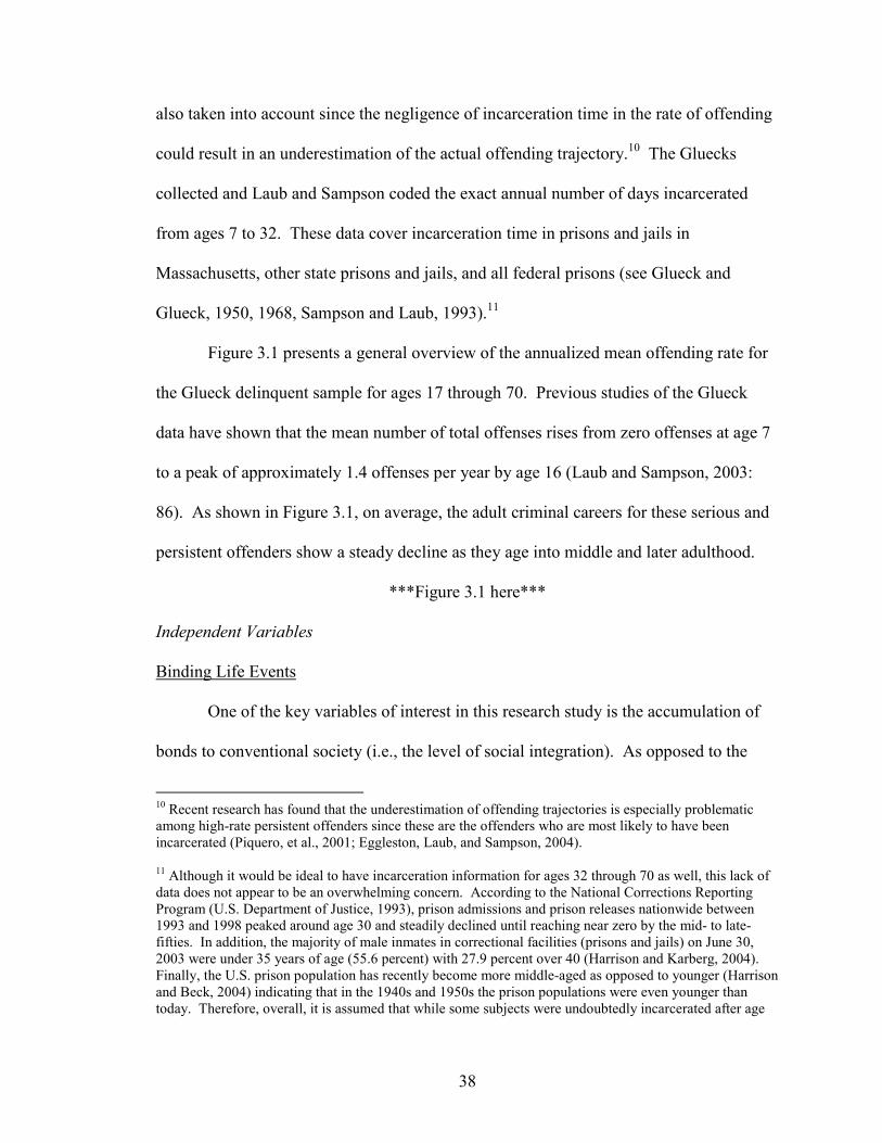
38
also taken into account since the negligence of incarceration time in the rate of offending
could result in an underestimation of the actual offending trajectory.10 The Gluecks
collected and Laub and Sampson coded the exact annual number of days incarcerated
from ages 7 to 32. These data cover incarceration time in prisons and jails in
Massachusetts, other state prisons and jails, and all federal prisons (see Glueck and
Glueck, 1950, 1968, Sampson and Laub, 1993).11
Figure 3.1 presents a general overview of the annualized mean offending rate for
the Glueck delinquent sample for ages 17 through 70. Previous studies of the Glueck
data have shown that the mean number of total offenses rises from zero offenses at age 7
to a peak of approximately 1.4 offenses per year by age 16 (Laub and Sampson, 2003:
86). As shown in Figure 3.1, on average, the adult criminal careers for these serious and
persistent offenders show a steady decline as they age into middle and later adulthood.
***Figure 3.1 here***
Independent Variables
Binding Life Events
One of the key variables of interest in this research study is the accumulation of
bonds to conventional society (i.e., the level of social integration). As opposed to the
10 Recent research has found that the underestimation of offending trajectories is especially problematic among high-rate persistent offenders since these are the offenders who are most likely to have been incarcerated (Piquero, et al., 2001; Eggleston, Laub, and Sampson, 2004). 11 Although it would be ideal to have incarceration information for ages 32 through 70 as well, this lack of data does not appear to be an overwhelming concern. According to the National Corrections Reporting Program (U.S. Department of Justice, 1993), prison admissions and prison releases nationwide between 1993 and 1998 peaked around age 30 and steadily declined until reaching near zero by the mid- to late-fifties. In addition, the majority of male inmates in correctional facilities (prisons and jails) on June 30, 2003 were under 35 years of age (55.6 percent) with 27.9 percent over 40 (Harrison and Karberg, 2004). Finally, the U.S. prison population has recently become more middle-aged as opposed to younger (Harrison and Beck, 2004) indicating that in the 1940s and 1950s the prison populations were even younger than today. Therefore, overall, it is assumed that while some subjects were undoubtedly incarcerated after age

39
occurrence of life events, the focus is on the quality of the social bond that stems from
various life events. As a group, the three high quality life events of a stable marriage,
stable employment, and an honorable discharge from military service are labeled
“binding” events. To be clear, while marriage, military service, and employment are all
life events, stable marriage, honorable military service, and stable employment are
binding life events since they bind a person to conventional society.
The quality of each life event measure is a dichotomous variable, sometimes
created from a continuous variable. This dichotomization strategy was adopted for a
number of reasons. First, in order to calculate the accumulation of life events that are
experienced as binding, it is advantageous to dichotomize the continuum of scores into
“binding” or “not binding” and then add these together to get the number of binding life
events experienced. Also, as outlined by Farrington and Loeber (2000), interaction
effects are more easily studied and interpreted with dichotomous data. Also, these
researchers found, as opposed to losing information by dichotomizing, there is a decrease
in classification error when there are fewer categories into which a person can be
assigned. Finally, Farrington and Loeber conclude that “dichotomization greatly
simplifies the presentation of results, yields findings that are easily understandable by a
wide audience, and shows no sign in our analyses of producing misleading conclusions”
(2000: 121). However, it cannot be assumed that there will be no substantive differences
between the dichotomous and continuous variables in this data specifically. Therefore,
the interaction analyses will be conducted multiple times with dichotomous and with
32, the impact of this lack of data is not a fatal flaw given the fact that prison populations decrease with age and were even younger 50 years ago than today.

40
continuous measures to safeguard against the possibility that the dichotomization
substantively affects the results.
Table 3.1 presents the summary statistics of the dichotomized life event measures.
First, in order to measure the quality of military service, those with an honorable
discharge from military service is used. The Gluecks collected data from Army and
Navy officials on whether the subject was discharged from these branches of the service
with an honorable or a dishonorable discharge. This binary variable is used to measure
the strength of military service with the assumption that those who experienced a
dishonorable discharge were not likely to have adapted well to their military experience.
***Table 3.1 here***
Next, marital attachment is measured for the time periods between ages 17 and 25
and again between ages 25 and 32. Marital attachment for ages 17 to 25 was originally
constructed by Sampson and Laub and is a composite measure of information taken at the
time of the age 25 interview regarding the conjugal relationship between the subject and
his spouse as well as his sense of marital responsibility (Sampson and Laub, 1993: 144).
The dichotomous measure for marital attachment indicates whether the subject was or
was not strongly attached to his wife during that wave. Subjects who were labeled as
attached were those who assumed their marital financial and emotional responsibilities
and those who were living together amicably with no thought of separation (see also
Glueck and Glueck, 1968: 84). Fifty-one percent of the married men experienced a
cohesive marriage between ages 17 and 25.
Marital attachment between 25 and 32, also constructed by Sampson and Laub, is
a standardized composite measure that describes the strength of the subject’s attachment

41
to his wife during this time period. This measure again includes the indicator of conjugal
relations plus a measure of family cohesion (i.e., the extent to which the family unit had
integrated interests and affection) (see Sampson and Laub, 1993: 144). This measure is
dichotomized to reflect a strong marital attachment or not. Those with a marital
attachment score at age 32 that was greater than zero were coded a 1 and those with a
marital attachment score less than zero were coded a 0, splitting the sample virtually in
half. The 49 percent of the married subjects who were labeled as attached for ages 25 to
32 were those who showed integrated family cohesion and were happily living together
with no thought of separation (see also Glueck and Glueck, 1968: 84).
With respect to employment, the measure of job stability was originally
constructed by Laub and Sampson from the Gluecks’ interviews. Job stability for ages
17 to 25 and 25 to 32 are measured by a composite of three standardized variables – 1)
employment status at the time of interview, 2) length of time employed at present or most
recent job, and 3) work habits (Sampson and Laub, 1993: 143-144). These composite job
stability measures were then dichotomized to reflect the presence of strong job stability
for each time period. Those with a job stability score greater than zero at age 25 were
coded a 1 and those with a job stability score less than zero at age 25 were coded a 0.
This dichotomization was repeated for the age 32 measures (see Table 3.1 for
descriptives on these measures). Overall, those who are labeled as having job stability
tended to be those who were employed at the time of interview, had reliable and
industrious work habits, were seen as an asset to their employer, and had been in their
most recent job for a longer period of time (48 percent for ages 17 to 25 and 37 percent
for ages 25 to 32).

42
Non-Binding Life Events
The fourth life event measured in this study is the “non-binding” life event of
length of juvenile incarceration. Although all of the delinquent boys were incarcerated as
juveniles by design, there is considerable variability in incarceration time during these
years (see Sampson and Laub, 1993; Sampson, Laub, and Eggleston, 2004). Overall,
length of juvenile incarceration ranges from just a few months to over seven years
incarcerated during the 10-year juvenile period (ages 7 to 17) with an average of about
1.5 years spent in reform school.
This continuous variable was dichotomized into 730 days or more (2 years or
more) and less than 730 days and labeled long-term juvenile incarceration and short-term
juvenile incarceration, respectively. The rationale for this cut-point is that two years or
more, whether the days are served consecutively or sporadically throughout ages 7 to 17,
represents a substantial amount of time spent in confinement and away from family and
the community, especially during this crucial developmental period. Thus, long-term
juvenile incarceration is viewed as a non-binding life event that may interact with self-
control and/or adolescent competence. Using this dichotomization technique, 26 percent
of the sample experienced “long-term” juvenile incarceration (see Table 3.1).12
Social Integration
The method used to measure social integration (i.e., the accumulation of social
bonds) is the binding life event scale, which ranges from 1 to 9 for both the 17 to 25
12 Additional analyses will also be conducted with cut points at the 25th and 50th percentiles to test the robustness of the results. Specifically, using the 25th percentile as a cut point, long-term juvenile incarceration is defined as 9 months or longer incarcerated between ages 7 and 17 and using the 50th percentile as a cut point, long-term juvenile incarceration is defined as 14 months or longer incarcerated between ages 7 and 17.

43
measures of social bonds and the 25 to 32 measures of social bonds. This scale is based
on the proportion of the number of life events experienced as binding divided by the
number of life events experienced, for the three possible binding life events. This
proportion quantifies the accumulation of bonds under the assumption that a higher
percentage of events experienced as binding corresponds to a higher level of social
integration. For instance, a person with two binding events out of two life events
experienced has a stronger bond to conventional society than someone who experienced
only one of three life events as binding. Using a proportion as opposed to the raw
number of binding life events experienced allows more cases to be retained in the sample
by allowing those who experienced 1, 2, or 3 life events to be included.
In the straight proportion, someone who experiences one life event and
experiences that event as binding has the same proportion (1.0) as someone who
experiences three life events and experiences all three of them as binding. Therefore,
according the straight proportion measure, these individuals would be treated as equally
bonded to conventional society. To account for the potential differences between these
two scenarios, the binding life event scale differentiates between those who may have the
same numerical proportion but who experience a different number of life events.13
Descriptive data for the proportion of binding life events and the binding life event scale
are displayed in Table 3.2. Those with zero life events experienced are treated as missing
and are controlled for in the analysis. The issue of missing cases is discussed next.
***Table 3.2 here***
13 It is an open question as to whether someone who experiences three out of three events as binding is “more bonded” to society than someone who experiences one out of one life event as binding. Therefore, the analyses are conducted using both the straight proportion and the binding life event scale.

44
The sample sizes are 396 men for the age 17 to 25 measures and 406 men for the
age 25 to 32 measures. There are several reasons for missing data as outlined in Table
3.3. First, there are 20 cases which were lost in the archival process, reducing the sample
size to 480 for both age periods.14 Second, there are those who are missing because they
died before the interview age or were not followed-up by the Glueck research team. For
the 17 to 25 measures, 18 men died before age 25 and 15 were not followed up at the age
25 interview. These numbers rise to 24 dead and 22 not followed up for the 25 to 32
measures. Third, there are those cases that are missing information on key variables at
ages 25 and/or 32. Specifically, 51 cases are missing for the age 17 to 25 measure and 28
cases are missing for the 25 to 32 measure. It appears that the majority of these cases
spent a vast amount of the sampling period incarcerated, and hence, the requisite
information needed for the binding life event scale was not assessed.
***Table 3.3 here***
Criminal Propensity and Prior Adult Crime
The present investigation proposes to analyze the Gluecks’ and Sampson and
Laub’s longitudinal data using various statistical methods. The most severe threat to
internal validity for this study is the selection bias inherent in the research design.
Following the analyses conducted in Crime in the Making, three strategies are undertaken
in this study to control for potential selection bias (see Sampson and Laub,1993: 149-
153). First, all of these analyses focus solely on the delinquent sample such that the
selection bias inherent in the design of the study is controlled. Second, the strategy to
control for potentially important early individual differences (i.e., propensity) based on
14 Previous analyses on these cases have found “nothing unusual” about them (Sampson and Laub, 1993: 270, note 6).

45
available information that is observed and recorded in the data set is employed.
Specifically, criminal propensity will be measured using two observed variables,
unofficial delinquency and juvenile arrests while free (ages 7 to 17).
Unofficial delinquency represents a composite measure of total self-, parent-, and
teacher-reported delinquency and misbehavior. This variable ranges from 1 to 26 with a
mean of 14.24 (s.d. = 4.16) and taps into early antisocial behavior that may not have been
identified in official records (Sampson and Laub, 1993: 50-53). The offending rate for
the juvenile years measures the arrests for total crime from ages 7 to 17, accounting for
incarceration time, and has a mean of .425, a standard deviation of .246, and ranges from
.06 to 1.85. While it is impossible to control for every potential individual difference and
childhood factor that may be correlated with criminal propensity, this combined strategy
taps into the between-individual differences with respect to criminal propensity that are
manifested in official and unofficial delinquent behavior. Therefore, any significant
relationships between the key variables of interest and adult offending patterns will be
less likely to be attributable solely to individual propensities towards crime and
misbehavior.
Third, past offending is the best predictor of future offending. Therefore, in order
to control for prior adult offending, the prior adult arrest rate is used. For the analyses
investigating the conditional effect of life events during ages 17 to 25, this control
variable is the young adult arrest rate for ages 17 to 25. This rate is the number of total
arrests while free during those eight years. The mean arrest rate for this time period is
1.61 offenses while free (s.d. = 2.78) although the arrest rates range from zero to 30
offenses while free. Similarly, the prior arrest rate between ages 25 and 32 is used in the

46
models that investigate the conditional effects of binding life events on short-term and
long-term offending past age 32. The arrest rate for this later time frame has a slightly
lower mean than the earlier adult period with a mean of 1.02 offenses while free (s.d. =
2.44), although there is again a vast range in values from zero to 29 arrests while free
over the late 20s and early 30s.
One potential concern with including juvenile criminal propensity measures and
prior adult crime is multicollinearity between these measures. However, this issue does
not appear to be a cause for concern in this study. First, the correlations between
unofficial delinquency and both adult arrest rate measures are not significant within the
delinquent sample.15 Second, while the correlations between the juvenile, young adult
(17 to 25) and later adult (25 to 32) arrest rate measures are significant, their magnitudes
are not large. For instance, the correlation between the juvenile and young adult arrest
rates is .158 (p = .001) and similarly, the correlation between the juvenile arrest and later
adult arrest is .198 (p = .000).
Self-Control
There has been a substantial amount of research on the measurement of self-
control such as whether it is a unidimensional scale or a multidimensional scale, and
whether the scale should be measured by attitudes or behaviors. For instance, while there
are exceptions (e.g., Longshore, et al., 1996), many studies have used Grasmick, et al’s
(1993) unidimensional scale and have agreed that it is indeed unidimensional using
traditional factor analysis methods. With respect to attitudinal versus behavioral scales,
15 Although there is no correlation between unofficial delinquency and these adult arrest rates (i.e., lambda measures), unofficial delinquency is correlated with percent arrested between ages 17 and 25 (r = .148, p < .01) and ages 25 and 32 (r = .158, p < .01). Unofficial delinquency is also correlated with the frequency of arrests for ages 17 to 25 (r = .168, p < .01) and ages 25 to 32 (r = .103, p < .05).

47
Gottfredson and Hirschi (1990) state that since self-control is not a personality trait, a
behavioral scale is best to use. However, critics state that using a behavioral scale raises
questions of tautology in that using the elements of criminal behavior to characterize the
elements of low self-control translates into crime predicting crime since low self-control
is posited to predict crime (Akers, 1991).
One group of researchers states, “behaviorally based scales of self-control
produce no advantage over cognitively based ones in the prediction of criminal/deviant
behavior” (Tittle, Ward, and Grasmick, 2003: 362-363). Similarly, Pratt and Cullen’s
(2000) meta-analysis of self-control studies found that low self-control strongly predicts
crime and analogous behavior regardless of whether an attitudinal or behavioral scale was
used, and whether the scale was Grasmick, et al’s scale or an alternative attitudinal scale.
In essence, while there is a great deal of debate surrounding the type of scale used to
measure self-control, the conclusion appears to be that the findings are robust with
several different types of measures (cf., Marcus, 2004).
In general, scales measuring low self-control, either behaviorally or attitudinally,
have tapped into traits such as impulsivity, risk-seeking, self-centeredness, irritability,
lack of persistence, inattention, hyperactivity, physical responses to conflict, and a low
tolerance for frustration (see, e.g., Wright, et al., 2001, Grasmick, et al., 1993, Longshore,
et al., 1996, Evans, et al., 1997). The measure of self-control used here draws on several
childhood and adolescent behavioral manifestations of low self-control assessed through
self-, parent-, and teacher-reports collected during the first wave of the Gluecks’ study
(Glueck and Glueck, 1950). This variable is a composite measure of four separate

48
behaviors, each measured as dichotomous variables and reverse coded so that higher
scores indicate higher self-control.
The first two components of the self-control variable are drawn from early
childhood measures that Sampson and Laub have used in prior research as indicators of
childhood predisposition toward disruptive behavior (see Sampson and Laub, 1993: 88).
The first is a variable originally created from the parent’s interview and labeled difficult
child. This variable distinguishes between children who were overly restless and irritable
from children who were not. The second early childhood variable measures the extent to
which a child engaged in violent temper tantrums and was predisposed to aggressiveness
and fighting. This variable reflects the tendency towards a physical response by the child
to difficult situations growing up. These measures tap into irritability, physicality, and
hyperactivity --- three characteristics that have been theorized to distinguish between
levels of self-control.
Two adolescent behavioral manifestations comprise the final components of the
self-control measure. These are 1) whether the parents reported that the one of the boy’s
bad habits at the first wave interview was smoking and 2) whether, according to teacher
reports and school records, he was a persistent truant as opposed to never or only
occasionally truant. 16 These variables were combined to create a behavioral scale of self-
control ranging from 0 to 4. The self-control measure was then reverse coded so that a
high score represents high self-control and a low score represents low self-control. While
16 Self-reported, teacher-reported, and parent-reported information are available on whether or not the boy smoked at the wave I interview. Since these three measures are strongly correlated at r = .498 or greater, only the parent-reported measure was selected. While the three sources of information were also available for whether the boy was truant or not, only the school records and teacher reports provided information on the frequency of truancy.

49
this measure of self-control is a scale constructed from behavioral indicators measured
during childhood and adolescence, the assumption is that self-control is stable throughout
childhood, adolescence, and adulthood. 17
For the total sample (delinquents and non-delinquents), the mean level of self-
control is 2.61 with a standard deviation of 1.22. The frequency distributions for the
delinquents and nondelinquents are presented separately in Table 3.4. It is clear that the
scale for the nondelinquent sample is skewed to the higher end, indicating a tendency
toward higher levels of self-control. Specifically, two percent of the nondelinquents
score a zero or one, the lowest levels of self-control, while 54 percent score a four,
indicating the highest level of self-control. In contrast, the delinquents, as a group, are
more prone to have lower self-control on the scale with 40 percent scoring a zero or one
and only 5 percent scoring a four. These differences in distribution are expected given
that these subjects were selected into the study based on their delinquent or
nondelinquent status.
***Table 3.4 here***
Before this measure can be confidently used in the following analyses, its
reliability and validity must be confirmed. Reliability is a concern when using any type
of data and reflects how well a number of items measure a single latent construct.
Cronbach’s alpha is a coefficient of reliability that indicates the inter-correlation between
the selected items and is commonly used to assess reliability. For the measure of low
self-control, the Cronbach’s alpha shows that this latent construct is reliable with an alpha
17 This is a plausible assumption given the amount of research on the longitudinal stability of personality traits. For instance, in an extensive study on this topic, Conley found that across trait, method, and occasion over a 19-year period, several traits, including impulse control, were “valid personality traits that

50
of .545, which is slightly low but comparable to self-control scales used in other
published studies (see, e.g., Wright, et al., 2001; Evans, et al., 1997).
Although it is impossible to conclude that a measure is 100 percent valid, one way
to check for construct validity is to see if the variable in question performs as expected.
First, self-control among the entire sample should be strongly correlated with whether a
case is in the delinquent sample or the nondelinquent sample, which it is (r = -.672, p =
.000) and the related overall measure of unofficial delinquency, which it is (r = -.730, p =
.000). Second, self-control among the delinquent sample should be correlated with
official crime into later adulthood. Indeed, the results from the correlation analyses show
that the self-control scale appears to have face validity as it is significantly correlated
with total arrests between ages 17 and 70 (r = -.125, p = .006), between ages 25 and 70 (r
= -.115, p = .012), and between ages 32 and 70 (r = -.100, p =.031). Third, an early age
of onset is commonly linked with low self-control and therefore this measure should be
correlated with early onset of serious misbehavior, which it is (r = .177, p = .000).
Moreover, while these measures are all significantly correlated, their magnitudes are not
extremely strong, indicating that the measure of self-control is tapping into a different
domain than crime itself.
Finally, self-control should be correlated with the binding life event scales
described previously. According to Gottfredson and Hirschi (1990), those with low self-
control are not only more likely to commit crime but also less likely to experience
binding life events (see also Wright, et al, 1999). The correlation between self control
and the binding life event scale between ages 17 and 25 is .108 (p = .033) and between
[were] longitudinally stable during the decades of adulthood” (1985: 1280) (see also, Moss and Susman, 1980).

51
ages 25 and 32 is .162 (p = .001). While these correlations with the binding life event
scales are again significant but relatively low in magnitude, it is impressive that this
measure, based on childhood and adolescent behaviors, continues to be correlated with
distal factors occurring decades later.
Since the delinquent sample is largely comprised of those with low self-control,
the cut-points for dichotomization are chosen from the distribution of the total sample
(delinquents and non-delinquents) and split at approximately the 50 percent mark. Thus,
for the delinquents, the scale is dichotomized into those with low self-control (75 percent)
who scored a 0, 1 or 2 on the full scale and those with high self-control (25 percent) who
scored a 3 or 4 on the full scale. The bottom of Table 3.4 presents the summary statistics
for this dichotomized measure.
One concern with using a measure of self-control among a sample of delinquents
is that there is much less within-group variation than when the entire sample is used.
However, given that the outcome of interest is desistance from crime, one must analyze
the within-group differences in future crime among those already delinquent. This
situation is a “catch-22” in that the solution is denied by the circumstances inherent in the
problem. Therefore, in an attempt to increase variability, several alternative
specifications will be used in the interaction analyses. One alternative specification
dichotomizes the scale based on the frequency distribution of the delinquent sample,
which results in 187 boys (40 percent) labeled as low self-control (scores of 0 or 1) and
284 boys (60 percent) labeled as high self-control (scores of 2, 3, or 4). Another
specification is the continuous scale which will also be used in an effort to detect an
interaction effect.

52
Adolescent Competence
The measure of adolescent competence in this study is derived from the measure
used by Laub and Sampson (1998) to predict the effects of adolescent competence on
long-term socioeconomic status among the Glueck men. Drawing on Clausen’s work
(1991, 1993), Laub and Sampson constructed a measure of adolescent competence that is
consistent with Clausen’s idea of planful competence (see Laub and Sampson, 1998: 93-
94). This measure is a composite of 6 factors. The first two factors tap into whether the
boy had academic or vocational ambitions, meaning a desire for further schooling or to
learn a specialized trade and assesses the boy’s planfulness in the use of money. This
variable also includes whether the boy was labeled as intellectual or conscientious during
the psychiatric interview. Finally, the boy’s attitude towards school and whether he
performed well on his grades as stated by his teacher are the final two elements. With
each component being a binary variable, this measure of adolescent competence ranges
from 0 to 6, has a mean of 1.99, and a standard deviation of 1.55 (N=905). The
frequency distributions for the delinquent and nondelinquent samples are presented in
Table 3.4. 18
Laub and Sampson (1998: 94) conducted several validity checks of their scale of
adolescent competence and found this measure to be valid. In addition, as with self-
control, adolescent competence among the entire sample should be strongly correlated
with whether a case is a delinquent or nondelinquent, which it is (r = -.477, p = .000) and
with the related overall measure of unofficial delinquency, which it is (r = -.513, p =
18 It should be noted that there are 42 missing cases among the delinquent sample for this variable, largely due to a lack of school attachment and adolescent ambition data. However, t-tests comparing the missing and non-missing cases did not reveal any significant differences with respect to childhood characteristics, school or family experiences, or juvenile offending.

53
.000). Specifically, for the sample of delinquents, adolescent competence is significantly
and negatively related to total arrests between ages 17 and 70 (r = -.164, p = .001), total
arrests between ages 25 and 70 (r = -.144, p = .002), and total arrests between ages 32
and 70 (r = -.105, p = .029). Finally, adolescent competence should be positively and
significantly correlated with self-control which it is (r = .106, p = .028). However,
although adolescent competence and self-control are related to each other, the magnitude
of the correlation is not strong indicating that these two measures have discriminant
validity as well and are thus, not one in the same.19
As seen with the self-control measure, the delinquents are more prone to have
lower adolescent competence due to the study design. Here, none of the delinquents
scored a six (the highest level of adolescent competence) and only 5 percent scored a four
or five (see Table 3.4). The cut-off points for dichotomization were again determined
from the distribution of the total sample, leaving 88 percent of the sample representing
those with low adolescent competence (scores of 0, 1 or 2) and 12 percent of the sample
representing those with high adolescent competence (scores of 3 or more). Again, this
measure of adolescent competence is assumed to be stable into adulthood. Table 3.4
presents the summary statistics for this dichotomized measure.
Again, there is a problem of variation in the adolescent competence measure
within the group of delinquents. Therefore, alternative specifications such as a second
dichotomous variable based on the frequency distribution of the delinquent sample is
used in the interaction analyses. Dichotomizing on the delinquent sample leaves 287
19 In addition, a factor analysis also indicates that these two variables are measuring separate constructs. On the total sample, two factors emerge with the self-control components loading on one factor and the adolescent competence component measures loading on the second factor.

54
boys (65 percent) labeled low in adolescent competence (scores of 0 and 1) and 151 boys
(35 percent) labeled high in adolescent competence (scores of 2 through 5). The
continuous adolescent competence variable is also used as an alternative specification.
ANALYSIS
The analytical models used to investigate the question of whether social
integration and/or person-situation interactions influence adult offending are the
semiparametric mixed Poisson model (SPMM) and the hierarchical linear model (HLM).
The semiparametric mixed Poisson model is a relatively recent statistical technique
developed by Daniel Nagin (1999, 2005) which allows a disaggregation of offending
trajectories to reveal variability in offending over time. This model assumes that the
population is comprised of discrete Poisson distributions with a λ rate of offending. In
essence, different groups of offenders are assumed to commit crimes, and desist, at
different rates. This procedure assigns each individual a posterior probability of
membership into each estimated trajectory group and then assigns each case to the group
that he or she is most likely to belong. The final result is a number of different groups
comprised of individuals who demonstrate similar patterns of offending over time.
Specifically, the group-based model used for offending count data is the
semiparametric mixed Poisson model, which estimates the predicted number of offenses
per year at each age for each trajectory group. Each developmental trajectory assumes a
quadratic (or cubic) relationship that links age and offending as illustrated by the
equation 2
210log itj
itjjj
it ageage βββλ ++= (1)

55
where jitλ is the predicted rate of offending for person i in group j for time period t, itAge
is the age of person i for time period t, 2itAge is the squared age of person i for time period
t, and the coefficients jjj and 210 ,, βββ structure the shape of the trajectory for each group j.
Although every individual in each group is constrained to the same slope and intercept of
that trajectory, these parameters, which determine the level and shape of the trajectory,
are free to vary by group (Nagin, 2005: 33).
The trajectory method estimates these model parameters using maximum
likelihood for a fixed number of groups. The optimal number of groups is determined by
the Bayesian Information Criterion (BIC) which can inform the selection of the best
model for comparison of both nested and unnested models (see D’Unger, et al, 1998;
Nagin, 1999). The BIC is estimated using the following equation
knLBIC *)log()log(2 +−= (2)
where L is the maximum likelihood, n is the sample size, and k is the number of model
parameters (Nagin, 2005: 64). Lastly, this procedure assigns each individual a
probability of membership in each group. This posterior probability is determined using
the equation
∑=j
ji
jii jYP
jYPYjP ππ
ˆ)(ˆˆ)(ˆ
)(ˆ (3)
where )(ˆ jYP i is the estimated probability of observing the actual offending behavior Yi
conditional on membership in group j for person i, and jπ̂ is the estimated proportion of
the population in group j (Nagin, 2005: 79). Based on these probabilities, each individual
is assigned to the group displaying the largest group assignment probability. In other

56
words, individuals are assigned to the group to which they are most likely to belong
based on their offending patterns.
The simplest model assumes that exposure time for everyone is equal. When
exposure time is not equal, a parameter that accounts for exposure time can be added to
Eq. (1) when estimating the predicted rate of offending. Thus, for the analyses that take
incarceration into account, the group-based model includes an incarceration parameter in
the estimation. This added parameter incorporates the amount of time each person spent
in the community each year. With this additional parameter, jitλ from Eq. (1) becomes a
weighted λ representing the predicted number of offenses that person i in group j would
have committed if he had been free for the entire time period t (i.e., 365 days of the year).
Nagin (2005) describes several diagnostics to better assure the user that the
selected model is adequately capturing the heterogeneity in the sample and not
identifying nonsensical groups. The first diagnostic is the average posterior probability
of assignment for each group. This measure reflects the accuracy or certainty of group
assignment. The closer the average posterior probability is to 1, the more certain a
researcher can be about the group assignment. Also, a simple comparison between the
group probabilities that are estimated for the population and the actual proportion of
individuals who are assigned to the group can be informative. The closer these
proportions are, the more adequate the model.
A related diagnostic is the odds of correct classification (OCC). Using the
average posterior probability and the estimated proportion of the population for each
group, the equation for the odds of correct classification, as detailed in Nagin (2005: 88),
is

57
∧
∧
−
−=
j
j
j
j
jAvePP
AvePP
OCC
ππ
1
1 (4)
The numerator represents the odds of a correct classification into group j based on the
maximum probability classification rule while the denominator is the odds of correct
classification into group j based on random chance. Therefore, the OCC, in essence,
measures the predictive capacity of the average probability of assignment beyond random
chance. The larger the OCC, the better the assignment accuracy.
The offending trajectories for six different time periods are estimated to identify
the short-term and long-term offending trajectory groups between ages 17 and 25, 17 and
70, 25 and 32, 25 and 70, 32 and 45, and 32 and 70. To begin the estimation process, an
incrementally larger number of groups are estimated and the optimal model is assessed
using the BIC statistic along with other model diagnostics such as population estimates
for each group and posterior probabilities of assignment.
The semiparametric group-based model assumes that the population is comprised
of discrete groups of offenders. Since this is an assumption that may or may not be true,
hierarchical linear modeling is also used which assumes that there is a continuous
distribution of trajectories rather than a multinomial distribution. This additional analysis
will safeguard against making conclusions based on possibly erroneous model
assumptions (see Bushway, Brame, and Paternoster, 1999).
Briefly, hierarchical linear modeling allows a simultaneous estimate of variations
in crime within individuals over time and between-individual differences in offending
patterns. To study individual change within the HLM framework, the crime counts for

58
each individual by age are viewed as nested within that individual. There are two levels
of analysis. Level 1 estimates each person’s development with a unique individual
growth trajectory that depends on a set of parameters. The growth parameters from Level
1 become the outcome variables in Level 2 of the model and are determined by person-
level characteristics. Therefore, Level 1 in the model estimates the within-individual
change and Level 2 in the model represents the between-individual analysis (Raudenbush
and Bryk, 2002).
At the within-individual level, crime is modeled as a quadratic function of age.
Specifically, a hierarchical Poisson model is used that incorporates incarceration when
available (i.e., time on the street) (Raudenbush, Bryk, and Congdon, 2004). Therefore,
the outcome variable in this model is the log of total offending per year (lambda). For the
models that include ages prior to age 32, the outcome variable is the log of the total
offending rate per year free (lambda*days free). The basic elements of this within-person
model are:
Log(Crimeit ) = π0i + π1i Ageit + π2i Age2it + eit, (5)
where i is the index for individuals and t stands for the longitudinal observations. The
intercept, π0i, is the estimated rate of crime when age is set to zero (i.e., initial status).
The π1i and π2i parameters estimate the average rate of change and rate of acceleration or
deceleration, respectively (Raudenbush and Bryk, 2002: 163). To increase the
meaningfulness of the interpretation of the intercept term, researchers use the technique
of centering their data. Centering at the mean provides a more meaningful anchor to
better understand the variation around the mean. Here I center age at the mean of the
observed age-person distribution (age 20.5 for the 17 to 25 model, age 28 for the 25 to 32

59
model, 38 for the 32 to 45 model, age 43 for the 17 to 70 model, age 47 for the 25 to 70
model, and age 50.5 for the 32 to 70 model).
At the between-individual level, the parameters from Level 1 are estimated from
the Level 2 equations. According to the model used in this analysis, the slope parameters
for age are allowed to vary across persons, as indicated by the error term but the
acceleration parameter is fixed.20 The basic elements of the between-individual model
are:
π0i = β00 + β01 X i + β02 Wi + β03 Zi + r0i (6)
π1i = β10 + r1i (7)
π2i = β20 (8)
where X, W, and Z represent the various individual-level and control variables described
previously that are presumed to predict patterns of crime over time (Raudenbush and
Bryk, 2002: 164). 21 The specific models for the different analyses are described next.
Cumulative Advantage/Social Integration
Sampson and Laub (1993) found that strong social bonds lead to a reduction in
criminal activity. Drawing on the cumulative advantage and social integration literatures,
the current study investigates whether there is a conditional effect of social bonds on
adult offending based on the amount of bonding a person has to society. Specifically, the
hypothesis is that those who are more socially integrated into society will have lower
levels of short-term and long-term offending and steeper rates of decline over the short-
and long-term than those who are less socially integrated. As outlined in the previous
20 In all of the analyses, the residual parameter variance for age-squared is set to zero. When this is free to vary, the model fails to converge. 21 The model results reported are the population-average model parameters with robust standard errors.

60
section, social integration is measured according to the binding life event scale where
high social integration is indicated by higher scores on the binding life event scale and
low social integration is indicated by lower scores on the scale. The longitudinal
methods of semiparametric mixed Poisson modeling and hierarchical linear modeling are
used to investigate these hypotheses.
In the case of the semiparametric mixed Poisson model, a multinomial logit
analysis within the semiparametric model is used which links individual characteristics to
the probability of group membership in order to test whether the individual-level
characteristics can predict group membership (Nagin, 2005: Chapter 6). In order to do
this, independent variables of interest (i.e., the binding life event scale score) and the
control variables are included, along with age, in the trajectory equation. The group
membership probability then follows a multinomial logit function. The specific question
then is: Controlling for criminal propensity and prior adult crime, does the binding life
event score predict trajectory group membership? If a higher binding life event scale
score significantly distinguishes between the offending trajectory groups whose levels
differ and/or rates of decline diverge, the implication would be that one condition of the
influence of life events on offending patterns is a person’s level of social integration.
With respect to the HLM analyses, social integration and the control variables are
included in the Level-2 model, along with age and age-squared at Level-1. For each
model, the Level-2 variables will be used to explain the variation in the intercept term,
which translates to explaining the rate or level of offending. Social integration will then
be entered as a Level-2 variable to explain variation in both the intercept term and in the
slope parameter, or rate of decline. If the social integration coefficient significantly

61
impacts the slope parameter, the control variables will also be entered into the Level-2
model. This modeling will allow an investigation into whether variation in social
integration is associated with variation in the rate of decline over the life course as well as
the level of offending.
Interactions
The exploratory hypothesis put forth with regard to the relationship between self-
control and adolescent competence and life events is that the effect of life events on
desistance from crime may depend on these individual characteristics. For instance, it is
hypothesized that those with lower self-control will be affected more from having
multiple binding life events of marital stability, job stability, and honorable military
service as measured by the binding life event scale than those with higher self-control. In
addition, those who experience long-term incarceration may also be affected differently
depending on their individual characteristics. Again, the focus in the interaction analyses
is on identifying different levels and rates of decline in future offending. Not only could
future offending levels be affected by social integration or long-term incarceration for
those with low self-control or low adolescent competence but the rates of change in
offending may also be affected.
To begin, as a global test, the interaction analyses will be conducted with self-
control or adolescent competence and the binding life event scale, using a variety of
specifications. First, a dichotomization of the binding life event scale for ages 17 to 25
and 25 to 32 is used to test whether interactive effects exist between social integration
and individual characteristics on adult offending. For each time period the binding life
event scale is divided into those whose proportion of binding life events to life events

62
experienced was 50 percent or less (i.e., a binding scale score of 1 through 5) and those
whose proportion of binding life events to life events experienced was over 50 percent
(i.e., a binding scale score of 6 through 9). This dichotomization results in 219 men
labeled low in social integration (55 percent) and 177 high in social integration (45
percent) between ages 17 and 25 and 246 men labeled low in social integration (61
percent) and 160 labeled high in social integration (39 percent) between ages 25 and 32.
Again the semiparametric mixed Poisson model and the hierarchical linear model
will be used to estimate these effects on short-term and long-term adult crime. Basically,
the same approach as described in the previous section is used for the interaction
analysis. The difference here is that, instead of modeling social integration only, an
interaction term of the binding life events scale and the individual characteristic and their
corresponding main effect variables are modeled as the variables of interest.
Specifically, the dichotomous social integration measure will be interacted with
the dichotomous individual characteristic measure described in Table 3.4 to estimate this
interaction effect on the short- and long-term levels of adult offending. These analyses
will then be replicated with the individual characteristic measure that was dichotomized
based on the delinquent sample as opposed to the total sample and replicated again with
the continuous individual characteristic measure and the continuous binding life events
scale. Depending on the results of these findings, evidence of an interactive effect will
then be investigated further to identify if a certain binding life event is the driving force
behind the interaction effect. Finally, if these analyses find evidence of interactions, the
conclusion would be that one condition of the influence of social bonds stemming from

63
life events on desistance is the individual characteristic of adolescent competence and/or
self-control.
In addition to a predicted interaction between binding life events and individual
characteristics, it is also predicted that the non-binding life event of long-term
incarceration and these individual characteristics will interact. For example, those with
low self-control may show amplification effects from long-term incarceration. In the
same vein, it is hypothesized that those with higher adolescent competence will be less
affected by long-term incarceration. Here, the time frame of the dependent variable shifts
to 17 to 25 for the short-term analysis and 17 to 70 for the long-term analysis since
juvenile incarceration ends at age 17 and everyone experienced this life event.
Multinomial logit analyses of the trajectory groupings from the semiparametric
mixed Poisson model and HLM analyses for these same time periods will be used to
examine the interactive effect for juvenile incarceration and self-control or adolescent
competence. Specifically, the dichotomous measure of juvenile incarceration described
in Table 3.1 will be interacted with the dichotomous self-control and adolescent
competence measures described in Table 3.4 to estimate the interaction effect on the
short- and long-term levels and rates of change in offending. Again, these analyses will
be replicated with the measures that were dichotomized based on the delinquent sample
as opposed to the total sample and the scale measures. The following chapters present
the results of the analyses described in this chapter.

64
CHAPTER 4: SOCIAL INTEGRATION AND DESISTANCE Drawing on the cumulative advantage and social integration literature discussed
in Chapter 2, one potential condition of desistance examined here is the accumulation of
life events and their subsequent social bonds (i.e., level of social integration). The
current research acknowledges Sampson and Laub’s finding that independent effects
exist between binding life events and desistance and further tests their theory by asking
whether the presence of additional social bonds to conventional society within the same
individual is related to lower levels and steeper rates of offending, in both the short- and
long-term. The expectation is that social integration will affect the level of offending and
rate of decline, controlling for criminal propensity and prior adult crime.
The semiparametric mixed Poisson models (SPMM) and hierarchical linear
models (HLM) are utilized to address the relationship between social integration and
short-term and long-term future offending in adulthood. For each time period, the
semiparametric trajectory model will be presented followed by the findings from the
multinomial logit comparisons with respect to the influence of social integration on the
offending trajectory groupings. The HLM models will then be presented for the
corresponding time period. As described in Chapter 3, social integration is
operationalized in two ways, the proportion of binding life events and the binding life
event scale. Since the substantive conclusions are the same regardless of the
operationalization of social integration, only the results using the binding life event scale
are presented.

65
SOCIAL INTEGRATION AND SHORT-TERM OFFENDING
Social Integration Between Ages 17 to 25
To begin, the influence of social integration measured between ages 17 and 25 on
short-term offending (ages 25 to 32) is examined. The semiparametric mixed Poisson
model estimated five groups to best describe the adult offending patterns for ages 25 to
32 for these delinquent boys. As displayed in Table 4.1, while the BIC statistic
continued to increase up to at least six groups, the five group model was selected on the
basis of parsimony and the model diagnostics described in Chapter 3. In essence, the
group-based method was no longer identifying substantively interesting groups past the
five groups identified. In addition, the group population and sample proportion were
similar, the average posterior probabilities were relatively high, and the odds of correct
classification were above the recommended number five for the five group model (see
Table 4.1).
***Table 4.1 here***
Figure 4.1 displays the five estimated offending trajectories for this time period.
The first group is labeled the “high-level declining offender” group who display high
levels of offending throughout this time period but begin decreasing in their rate of
offending around age 28.22 The second group, the “low-level declining offenders,” begin
at a much lower rate than their high-level counterparts and decline to a near zero rate of
offending by age 32. The “inclining offenders” in this model begin at a relatively low
rate of offending at age 25 but nearly triple their rate of offending by age 32. The “low-
22 It should be noted that the group labels used in each model are not meant to reflect groups that occur in reality. The technique is used as a heuristic device to cluster the data with respect to their developmental trajectories over time. Also, these labels are assigned relative to other groups in the sample. For instance, the label “high-level declining offender” is relative to others in this delinquent sample.

66
level offenders” and “nonoffenders” display somewhat parallel trajectories with the low-
level offenders committing a very low but non-zero rate of offending from ages 25 to 32.
***Figure 4.1 here***
Simple univariate chi-square and ANOVA tests reveal that there is a significant
relationship between the binding life event scale score and these semiparametric
offending trajectory groups (data not shown). 23 However, while the chi-square and
ANOVA tests begin to identify these relationships through an analysis of group mean
differences, these are univariate tests that do not control for other important factors that
may be influencing group differences, such as criminal propensity. Therefore,
multinomial logit analyses that include a control for criminal propensity and prior adult
crime is employed.
The multinomial logit analysis results for the effect of social integration between
ages 17 and 25 on short-term adult offending between ages 25 and 32 are presented in
Table 4.2. One pattern that emerges in these comparisons is that the binding life event
scale significantly distinguishes between each of the trajectory groups that are still
offending between ages 25 and 32 and the group that is not offending during this adult
period. Based on the negative direction of the significant binding life event scale
coefficients in these comparisons (i.e., -.2983, -.3791, -1.099, and -.4367), more socially
integrated individuals are associated with a lower likelihood of being classified into an
23 As expected, these findings correspond with a decrease in the mean binding life event score by trajectory group. For instance, in the 25 to 32 model, nonoffenders average a score of 5.885, low-level offenders average a score of 4.853, inclining offenders average a score of 3.840, low-level declining offenders average a score of 3.535, and the high-level declining offender group average a score of only 2.625. Similarly, the mean proportion of life events experienced as binding ranged from .69 for nonoffenders to .05 for high-level declining offenders.

67
offender group as opposed to the nonoffender group, controlling for official and
unofficial juvenile offending and prior adult crime.
***Table 4.2 here***
In order to interpret these results, the coefficients can be converted into predicted
probabilities of group membership within the semiparametric mixed Poisson framework
for different levels of social integration (Nagin, 2005: Chapter 6). After setting the
controls at their mean, the predicted probability of being classified as a high-level
declining offender with a binding life event score of 1 (low social integration) is .290. In
contrast, the predicted probability of being classified as a nonoffender with low social
integration is .005. For those with high social integration (binding life event score of 9),
these probabilities of membership drop to .001 for high-level declining offenders and rise
to .103 for nonoffenders.24 This same pattern exists for the remaining offender group
comparisons with the nonoffender group as well.
In addition, a similar pattern appears between high-level offenders and low-level
offenders. Here, a lower binding life event score significantly corresponds to being
assigned to the high-level declining group as opposed to being classified into any of the
other three offending groups. For instance, the significant coefficient of -.8006 for the
binding life event scale in the comparison between the high-level declining group and the
low-level offenders indicates that those with higher levels of social integration are more
likely to be low-level offenders between ages 25 and 32. Again this coefficient can be
translated into predicted probabilities with the controls set at their mean values. Here,
24 Since these probabilities are dependent on the population base rates for each group and on holding the control variables at their mean, the shift in probability with changing levels of social integration rather than the numerical magnitude of the probability is emphasized.

68
while the predicted probabilities of membership fall from .290 to .001 as high-level
declining offenders move from the lowest to highest levels of social integration, the
predicted probabilities of membership for low-level offenders rises from .384 to .676 as
the level of social integration increases from low to high.
One additional comparison of note in Table 4.2 is between the inclining group and
the high-level declining group --- the two groups with drastically different slopes of
offending between ages 25 and 32. As the significant coefficient of -.7198 indicates,
higher social integration is associated with a higher likelihood of being in the inclining
group when compared to the high-level declining group. In other words, a person with
high social integration is more likely to be in the lower-level but increasing offending
group (inclining offender) when compared to the higher-level yet decreasing group (high-
level declining offender). This suggests that social integration is a better predictor of
offending level than rate of change in offending.
To show the overall pattern of the differing predicted probabilities, Figure 4.2
displays the hypothetical impact of increasing the binding life event scale score on the
probability of belonging to each group, holding the control variables in the model at their
means. For ease of comparison, the predicted probabilities of belonging to the inclining
offenders and low-level declining offenders have been combined as well as the low-level
and nonoffenders. Overall, there is a clear decrease in probability for those in the high-
level declining offender group and a sharp increase in probability of being assigned to
either the nonoffender or low-level offender groups as the level of social integration
increases. For instance, a score of 1 corresponds to a .390 chance of being in the
nonoffender or low-level offender groups. This probability doubles to .779 if a person

69
were to experience a binding life event scale score of 9 (i.e., experiencing marital
attachment, honorable military service, and stable employment between ages 17 and 25).
This is in stark contrast to the predicted decrease of membership probability in the high-
level declining offender group as the level of social integration increases, again with the
controls set at their mean.
***Figure 4.2 here***
The results of social integration between ages 17 and 25 on short-term offending
(ages 25 to 32) from the HLM analysis concur with the multinomial logit model results.
Again, the binding life event scale significantly affects the levels of offending in the
short-term. From the unconditional model in Table 4.3, it is evident that the average total
offending rate is .68 crimes while free at age 28 (e-6.291 * 365) and the average rate of
decline is 6 percent per year as indicated by the age-slope coefficient ((e-.0616 – 1)*100).25
The conditional model, introduces the binding life event scale, criminal propensity, and
prior adult arrest as explanatory variables for the intercept parameter.26 The level of
social integration significantly affects the level of offending as indicated by the
significant coefficient of -.2263 in the Level-2 model. Thus, a unit increase in the
binding life event score is associated with having a predicted 20 percent lower level of
offending at age 28. Again, this is especially convincing since this model controls for
criminal propensity and prior adult crime. With respect to whether social integration
affects the rate of decline in short-term offending, a conditional model which included the
25 The correlation between the initial status and growth rate coefficients is .186. This positive correlation indicates that those with a higher level of offending at age 28 decline at a faster rate per year. 26 The reliability of the initial status parameter is .697 signaling that much of the variability in the estimate is due to systematic error as opposed to model error (Raudenbush and Bryk, 2002: 165-166). This indicates that the addition of Level-2 variables for the age parameter is warranted.

70
social integration measure as an explanatory variable for the slope parameter was
analyzed. The binding life event scale score was not significant.27 The non-significance
of this coefficient indicates that a person’s level of social integration has no effect on his
rate of decline in the short-term (data not shown).
***Table 4.3 here***
Social Integration Between Ages 25 and 32
When the focus is on social integration measured between ages 25 and 32 on
short-term offending between ages 32 and 45, a similar story emerges. Here, the
semiparametric mixed Poisson model identifies four groups to best describe short-term
adult offending patterns. Again, while the BIC statistic continued to increase up to six
groups, the four group model was chosen based on the group population and sample
proportion comparisons, the average posterior probabilities, the odds of correct
classification, and parsimony (see Table 4.4).
***Table 4.4 here***
As Figure 4.3 indicates, these different patterns predominantly show variation in
levels of offending as opposed to variation in change patterns over this time period. The
“high-level offenders” commit more offenses on average than the “mid-level offenders”
who in turn commit more offenses per year than the “low-level offenders.” Finally, these
three groups all commit more offenses than the “nonoffender” group who commit
virtually zero offenses throughout this time frame.
***Figure 4.3 here***
27 The reliability of the growth parameter is .281 signaling that much of the variability in the estimate is due to model error as opposed to systematic error making the finding of significance for this level-2 variable unlikely (Raudenbush and Bryk, 2002: 165-166).

71
The multinomial logit results indicate a very similar story to that described above.
Therefore, these results will be described but not presented in tabular form. Here, the
binding life event scale score significantly distinguishes between the offender groups and
the nonoffender group depicted in Figure 4.3, controlling for criminal propensity and
prior adult crime. The main difference between the results of social integration measured
between ages 25 and 32 and the results of social integration measured between ages 17
and 25 on short-term offending detailed above, is that there are no significant differences
between the different levels of offending. The lack of significance between the high-
level offender group and the remaining groups is likely due to the fact that the sample
size for the high-level offender group is very low (N = 15). However, this explanation is
not likely to be the reason for the nonsignificant finding between the mid-level and low-
level offenders.
The HLM analysis of the influence of social integration (age 25 to 32) on short-
term offending is virtually identical to that described above for the social integration (age
17 to 25) analyses on short-term offending (data not shown). Here, a higher level of
social integration is associated with a 14 percent lower level of offending at age 38,
controlling for criminal propensity and prior adult arrest. In addition, as seen in the
earlier analyses, social integration does not significantly affect the rate of decline in
short-term offending.28
Summary of Short-Term Results
Overall, there is consistent evidence in the short-term models that levels of total
offending are significantly influenced by the level of social integration a person
28 The reliabilities for the initial status and growth parameters in these models are .696 and .286, respectively. The correlation between these two parameters is .271.

72
experiences in their recent past. This is especially apparent between offenders and
nonoffenders but is also true, although less consistently so, between different groups of
offenders. Finally, there is consistent evidence from these analyses that the rates of
decline are not significantly affected by a person’s level of social integration. We move
next to an examination of long-term adult offending to see if a person’s level of social
integration in early adulthood continues to affect their offending over the entire life
course.
SOCIAL INTEGRATION AND LONG-TERM OFFENDING
Social Integration Between Ages 17 and 25
When the trajectory groups are estimated over the long-term from ages 25 to 70,
four groups of offenders with different rates of offending are identified. Again, based on
parsimony and the model diagnostics, four groups were estimated even though the BIC
continued to increase up to six groups (see Table 4.5). The four trajectory patterns in
this model are displayed in Figure 4.4. The “high-level late declining offender” group
displays high levels of offending throughout most of adulthood. Beginning in their late
30s, they show a steady rate of decline before terminating their offending in late
adulthood. The “high-level declining offender” group also displays a high level of
offending in their late 20s but declines at a much faster rate than the high-level late
declining offenders. The “low-level declining offenders” display a desisting pathway in
early adulthood that again somewhat parallels the nonoffenders. Finally, the adult
“nonoffenders” trajectory describes the offending patterns of those delinquent boys who
have the lowest rate of offending in their twenties and who, for all intents and purposes,

73
have desisted by their early 40s. While these men do not literally exhibit zero offenses in
each year, they are considered nonoffenders relative to the other groups and labeled as
such for the sake of consistency across models.
***Table 4.5 here***
***Figure 4.4 here***
The analyses of the long-term impact of social integration on offending are
somewhat inconsistent with each other making any concrete conclusions problematic.
First, in the multinomial logit analysis of the offending trajectories from ages 25 to 70,
the binding life event scale, measured between ages 17 and 25, inconsistently predicts
group membership between offenders and nonoffenders and between different levels of
offenders. As Table 4.6 indicates, only two of the six comparisons are statistically
significant. Here, the level of social integration significantly distinguishes membership
between the high-level declining offender and the nonoffender or low-level declining
offender groups, after controlling for criminal propensity and prior adult crime. Again,
the lack of significance between the high-level late declining group and the other three
groups may be due to the fact that the sample size for the high-level late declining group
is very low (see Nagin, 2005: 109). However, this explanation is not likely to be the
reason for the nonsignificant finding between the low-level declining offenders and the
nonoffender group.
***Table 4.6 here***
Second, the multinomial logit results indicate that social integration does not seem
to affect rates of decline over the life course. This conclusion stems from the lack of
significant difference between the high-level late declining offenders and the high-level

74
declining offenders --- the two groups who both begin at high rates of offending at age 25
but who desist at very different rates of decline over the life course. However, this lack
of significance again may be a function of the low population base rate of 3.3 percent and
low sample size for the high-level late declining group.
Figure 4.5 displays the overall impact of increasing social integration on
trajectory group membership probabilities. This figure clearly depicts the decrease in
probability for those in the high-level declining group and the increase in probability of
being assigned to the nonoffender and the low-level declining group as the level of social
integration increases. For instance, after setting the controls to their means, the predicted
probability of being classified as a high-level declining offender between ages 25 and 70
with a binding life event score of 1 is .416. This probability falls to .067 for those with a
binding life event score of 9. This trend is drastically different than the one seen with the
nonoffender group. For this group, experiencing zero of the three life events as binding
between ages 17 and 25 (i.e., a score of 1) is associated with a .218 probability of being
classified as a nonoffender between ages 25 and 70. This probability of group
membership rises to .469 when a person experiences a stable marriage, honorable
military service, and stable employment (i.e., a score of 9). What is also clear is the
similarity in trends between the nonoffenders and the low-level declining offenders as
well as the stability of the high-level late declining offender group across the different
levels of social integration.
***Figure 4.5 here***
Overall, there appears to be some evidence to suggest that the binding life event
scale predicts between offenders and nonoffenders and between different offender groups

75
in the long-term. However, this evidence is not consistent across all models or all
comparisons. To investigate this further, a logistic regression that combines all offender
groups into one group and compares them to the nonoffender group shows that, indeed, a
higher level of social integration is associated with being a nonoffender as opposed to an
offender, after controlling for criminal propensity and prior adult crime (see Table 4.7).
A separate logistic comparison between the high-level and low-level groups of offenders
(i.e., the two high-level declining offender groups versus the low-level declining offender
group) displayed at the bottom of Table 4.7 also shows a significant impact of social
integration. Taken together, these findings indicate that while there is inconsistent
evidence that social integration affects levels of offending individually, the aggregate
logistic analyses show that social integration does predict differences among offenders
and nonoffenders and among high- and low-level offenders in the long-term.
***Table 4.7 here***
The HLM results for long-term offending are presented in Table 4.8 and show
evidence both consistent and inconsistent with these results. To begin, the average total
offending rate in the unconditional model is .13 crimes while free at age 47 (e-7.925 * 365)
and the average rate of decline is 9 percent per year.29 Model I, the first conditional
model, introduces the binding life events scale score for ages 17 to 25 and the control
variables for criminal propensity and prior adult crime.30 The significant coefficient of -
.1599 for the binding life event scale indicates that those with a higher level of social
29 The correlation between the initial status and growth parameters is .536, indicating that those who have a higher level of offending at age 47 decline at a faster rate per year. 30 The reliability of the initial status parameter is .639 signaling that including level-2 variables to explain the variability in the estimate is warranted (Raudenbush and Bryk, 2002: 165-166).

76
integration between ages 17 and 25 have a 15 percent lower level of offending at age 47.
Next, in Model II, the level of social integration and the control variables are added as
Level-2 explanatory variables to the slope parameter.31 In contrast to the short-term
models, the impact of social integration on the rate of decline in this long-term model
indicates that higher levels of social integration significantly correspond with a faster rate
of decline.32 In this final model, the significant intercept and growth rate coefficients for
the binding life event scale indicate a 5 percent lower level of offending at age 47 and a
one percent faster rate of decline for those with a unit increase in level of social
integration, after controlling for criminal propensity and prior adult arrest. Thus,
according to this model, social integration affects both the level of offending and the rate
of decline over time in the long-term.
***Table 4.8 here***
Social Integration Between Ages 25 and 32
Finally, five groups were estimated to best describe the long-term adult offending
patterns from ages 32 to 70. The model diagnostics are presented in Table 4.9. Again,
the five group model was chosen based on the group population and sample proportion
comparisons, the average posterior probabilities, the odds of correct classification, and
parsimony.
***Table 4.9 here***
The offending trajectories for this five group model are displayed in Figure 4.6.
The first group is labeled the “high-level late declining offender” group who display high
31 The reliability of the growth parameter is .451. 32 This is true in models with and without the controls added (data not shown).

77
levels of offending throughout the time frame and slowly begin to decrease their rate of
offending around age 40. The second group, the “high-level declining offender” group
offends at a higher rate at age 32 than the high-level late declining group but is already on
a downward trajectory at this age and terminates offending in their early 50s. The third
and fourth groups are labeled the “low-level declining offenders I and II,” and display
parallel trajectories. These two groups both begin at a much lower rate of offending at
age 32 than their high-level counterparts and slowly decline in their offending over the
life course. The low-level declining offender I group continues offending at a non-zero
rate into late adulthood while the low-level declining offender II group decline to a near
zero rate of offending by around age 50. Finally, there is the “nonoffender” group who
for all intents and purposes refrain from offending throughout this time period.
***Figure 4.6 here***
The overall story of the influence of social integration on long-term offending
becomes even less clear when the focus is on the influence of social integration between
ages 25 and 32 on offending trajectories between 32 and 70. Here, the multinomial logit
model reveals that levels of social integration only significantly distinguish between one
group of offenders and the nonoffenders. Therefore, on the whole, it does not distinguish
between offenders and nonoffenders or between levels of offenders (data not shown).
Similar to the long-term analysis of social integration between ages 17 and 25 described
above, logistic regression analyses were conducted to further investigate this lack of
significant findings. These results are displayed in Table 4.10.
***Table 4.10 here***

78
A comparison between the four offender groups combined and the nonoffender
group reveals that higher levels of social integration between ages 25 and 32 are
associated with being a nonoffender, controlling for criminal propensity and prior adult
crime. However, a similar logistic analysis which combines the two high-level groups
and the two low-level declining groups (and excludes the nonoffenders) finds a
nonsignificant effect of social integration on long-term offending groups. Therefore,
while an aggregation of groups indicates that social integration appears to predict
between offenders and nonoffenders, it does not show that social integration predicts
differences in levels of offending among offenders over the entire life course. However,
the sample size of high-level offenders is still quite small (N=21) (see Table 4.10).
Thus, we move next to the HLM analysis which assumes a continuous
distribution of offending trajectories as opposed to a multinomial distribution. In this
model, higher levels of social integration between ages 25 and 32 is significantly related
to lower levels of offending in the long-term (data not shown). Here, a higher level of
social integration is associated with a 13 percent lower level of offending at age 50.5,
controlling for criminal propensity and prior adult crime.
Finally, social integration measured between ages 25 to 32 does not seem to affect
rates of decline over the life course. First, the multinomial logit results for the 32 to 70
models indicate that the binding life event scale does not distinguish between the two
groups offending at high levels at the beginning of the time period but declining at
different rates across the life course (i.e., the high-level late and high-level declining
offender groups in Figure 4.6) (data not shown). However, again, this is likely due to the
small sample sizes of these two groups (N = 11 and 10, respectively). Second, in the

79
HLM model for social integration measured between ages 25 and 32, unlike in the earlier
long-term HLM analyses in Table 4.8, the HLM analyses of social integration between
ages 25 and 32 finds that the rate of decline is not significantly impacted by the binding
life event score (data not shown).
Summary of Long-Term Results
In sum, the results from the long-term analyses are less consistent than those seen
in the short-term analyses. First, the evidence from the multinomial logit analyses
indicates that while social integration significantly predicts differences in offenders and
nonoffenders, these differences are only found in some of the individual comparisons.
The aggregated logistic analyses, however, do consistently show that social integration
predicts the probability of being classified as an adult offender. Second, although the
HLM analyses found evidence that social integration predicts levels of offending, the
evidence from the multinomial logit models indicate that social integration does not
consistently predict between different offender groups, controlling for criminal
propensity and prior adult offending. Moreover, in the aggregate logistic regression
models, while social integration between ages 17 and 25 distinguishes between high-level
and low-level offenders, this finding was not true when social integration between ages
25 and 32 was analyzed. However, this again may be due to the small number of high-
level offenders. Third, the bulk of the evidence indicates that there is no effect of social
integration on the rate of decline. Although the long-term HLM analysis for social
integration between ages 17 and 25 indicates otherwise, this finding did not emerge in the
25 to 32 HLM analyses or in either multinomial analyses.33
33 However, less weight is placed on the multinomial results due to the fact that the lack of significant findings is likely an artifact of small sample sizes.

80
Taken together, the more conservative conclusion is that social integration
consistently predicts between offending and nonoffending in the long-term but only
sometimes predicts between levels of offending and rarely predicts rates of decline
among those still offending throughout the life course. The apparent inconsistency found
in these long-term analyses could be a result of the general difficulty of predicting long-
term outcomes. Therefore, social integration may simply be better able to predict short-
term offending patterns as opposed to predicting offending into old age. One piece of
evidence to support this conclusion is that the amount of variation explained in the short-
term HLM models were 39 percent and 23 percent for social integration at 17 to 25 and
25 to 32, respectively while these percentages in the long-term HLM models fell to 8
percent and 15 percent, respectively.
CONCLUSION
The general conclusion from these analyses is that social integration is
significantly related to a reduction in offending over time, at least in the short-term. This
finding is in agreement with Sampson and Laub’s theory of age-graded informal social
control. In addition, this conclusion extends their previous finding that binding life
events have independent effects on the reduction of offending by showing that the
concentration of social bonds within the same individual is related to lower levels of
offending. It is important to note that these effects are evident even after controlling for
criminal propensity and prior adult crime, which increases the level of confidence that
levels of social integration inhibit crime.

81
CHAPTER 5: PERSON-SITUATION INTERACTIONS AND
DESISTANCE A second potential “condition” of life events on desistance is the interaction
between pre-existing individual characteristics and life events and their subsequent social
bonds. While there have been calls to investigate person-situation interactions in
criminology, few researchers directly test the types of questions posed in this study. In
the current study, both self-control and adolescent competence are explored as potential
moderators between the binding life events of a cohesive marriage, a stable job, and
honorable military service on future criminal offending. The expectation is that those
with low self-control and/or low adolescent competence will benefit more from being
socially integrated resulting in a greater reduction in future crime. In addition, this study
explores self-control and adolescent competence as potential moderators between the
non-binding life event of long-term juvenile incarceration, defined as two years or more
spent in reform school between ages 7 and 17, and criminal offending. The hypothesis
here is that long-term juvenile offending may encourage future crime among those with
low self-control leading to a subsequent increase or stabilization in criminal offending.
Or, a juvenile with a high level of adolescent competence may be more resilient in the
face of long-term juvenile incarceration.
INTERACTIONS OF SOCIAL INTEGRATION ON ADULT OFFENDING
First, the interaction effects between social integration and each individual
characteristic were investigated using semiparametric mixed Poisson modeling (SPMM)
and hierarchical linear modeling (HLM). While the intention was to use the short-term

82
and long-term semiparametric trajectory models depicted in Figures 4.1, 4.3, 4.4, and 4.6
to assess whether interaction effects were present, a number of the comparisons in the
multinomial logit analyses reported very large standard errors. This was often true
regardless of the specification of interaction used.
Therefore, to increase the stability of the analyses, logistic regressions were
conducted to compare the offender groups as a whole against the nonoffender group. For
instance, for the 25 to 32 offending trajectory model depicted in Figure 4.1, the high-level
declining offenders, low-level declining offenders, inclining offenders, and low-level
offenders were combined into one group of adult offenders and compared to the
nonoffender group. The standard errors in these analyses were more reasonable and
concurred with the substantive conclusions from the multinomial logit analyses.
Therefore, the logistic regression results are reported here as opposed to the individual
group comparisons. In addition, due to the consistency of the findings from the various
models and alternative specifications of the independent variables, only a representation
of the results are presented in tabular form.
To begin to understand the relationship between social integration and the
individual characteristics studied here, each model was first estimated without the control
variables included. While the measure of social integration significantly predicts adult
offending, the majority of the analyses showed no significant main effects for the
individual characteristic of interest and no significant interactions effects. As a next step,
several specifications of the analyses were conducted (as outlined in Chapter 3). First,
the dichotomous social integration measure was interacted with the dichotomous
individual characteristic measures described in Table 3.4 to estimate the interaction effect

83
on the short- and long-term levels of adult offending. Specifically, the multinomial logit,
the logistic, and the HLM analyses were conducted for the interaction between social
integration between ages 17 to 25 on short-term and long-term offending (ages 25 to 32
and 25 to 70, respectively) as well as for the interaction between social integration
between ages 25 to 32 on short-term and long-term offending (ages 32 to 45 and 32 to 70,
respectively). The results from the logistic and HLM analyses are presented in this
chapter.
Second, to safeguard against drawing false conclusions due the dichotomization
techniques employed here, these multinomial logit, logistic, and HLM analyses were then
replicated using the individual characteristic measure that was dichotomized based on the
delinquent sample as opposed to the total sample. These models were replicated a third
time using the continuous individual characteristic measure and the continuous binding
life events scale. Finally, when evidence of an interactive effect emerged, additional
analyses were conducted to examine the interactions between each individual life event
and the individual characteristic to test for the robustness of the results.
Interactions Between Social Integration and Self-Control
The question investigated here is, among those who experience high social
integration, do those low in self-control display different offending patterns than those
high in self-control? Based on extensive analyses, the answer to this question is no. For
example, the logistic regression analyses of social integration and self-control for the
offender groups and the nonoffender group reveal no interaction effects. The logistic
regression coefficient is interpreted as the change in the log of the odds of offending
associated with a one-unit increase in the independent variable. Through mathematical

84
manipulation of the full equation, predicted probabilities can be calculated (Liao, 1994).
One purpose of interpreting predicted probabilities based on different hypothetical
characteristics is to better understand the magnitude of the effect of social integration on
adult offending among those low or high in self-control. In addition, the effect of the
interaction coefficient and the direct effects of the component variables of the interaction
term should be interpreted as a system which the predicted probabilities allow (Jaccard,
Turrisi, and Wan, 1990).
Table 5.1 displays the results of the logistic regression for social integration (age
17 to 25) and self-control on short- and long-term adult offending (age 25 to 32 and 25 to
70, respectively). As mentioned above, the adult offender group for the short-term model
consists of those classified as high-level declining offenders, low-level declining
offenders, inclining offenders, and low-level offenders (see Figure 4.1). As Table 5.1
indicates, social integration significantly distinguishes between being in an adult offender
group and being classified as a nonoffender in both the short- and long-term. In addition,
there are no significant interactions between social integration and self-control on adult
offending probability. For instance, in the short-term model, with the control variables
held at their mean, someone who is high in social integration and high in self-control has
a 53 percent predicted probability of being an adult offender. This is compared to a 46
percent probability of adult offending for someone who is high in social integration but
low in self-control, which is not a substantial difference. Therefore, the key finding here
is that among those with high social integration, there is no significant difference in the
probability of being an adult offender based on levels of self-control. Not surprisingly,

85
those low in social integration and low in self-control have the highest probability of
being classified into one of the offending groups (77 percent).
***Table 5.1 here***
When the offending trajectory is expanded into late adulthood, as shown in the
bottom of Table 5.1, the probabilities of being classified as an adult offender are similar
to those seen in the short-term models. Here the adult offender group consists of those
classified as high-level late declining offenders, high-level declining offenders, and low-
level declining offenders (see Figure 4.4). In the long-term model, among those high in
social integration, a person high in self-control has virtually the same probability of being
classified as an adult offender as a person low in self-control (43 percent and 46 percent,
respectively). Those low in social integration and low in self-control again have the
highest probability of being classified into one of the offending groups with a 64 percent
chance.34
Logistic regression, however, cannot test whether there are interactive effects in
distinguishing levels of offending since it is a comparison between being classified as an
offender or an nonoffender. To examine the data in a different way, the hierarchical
linear models are employed. The results concur with those seen in the logistic analyses
and reveal no significant interactions between social integration (age 17 to 25) and self-
control on short- or long-term adult offending (ages 25 to 32 and 25 to 70, respectively)
(see Table 5.2).35 Using the HLM mixed model it is possible to calculate predicted mean
34 To safeguard against false conclusions due to potential multicollinearity between the self-control measure and the unofficial delinquency measure, additional analyses were conducted which omitted unofficial delinquency from the model. The findings from these analyses are similar with respect to significance, direction, and magnitude of the coefficients. 35 The reliabilities for the initial status and growth parameters in the short-term model are .590 and .278, respectively. The correlation between these two parameters is .233. The reliabilities for the initial status

86
rates of offending while free for different hypothetical values to better understand the
results and to interpret the main effects and interactions as a system. Here, with the
controls set to their mean values, at age 28 those with high social integration and low
self-control are predicted to commit .92 offenses per year free while those high in both
social integration and self-control are predicted to commit .70 offenses per year free.
These two rates are neither statistically significant nor substantively different especially
when compared to the rates for those low in social integration (2.88 and 2.13 for those
with low and high self-control, respectively).
***Table 5.2 here***
An identical story emerges when the time frame is expanded to age 70 with
respect to interactions between self-control and social integration. First, as the significant
and negative coefficient for social integration in Table 5.2 indicates, in the long-term
those with high social integration are predicted to commit fewer crimes per year at age 47
than those with low social integration. However, the lack of a significant interaction
coefficient indicates that this effect is the same regardless of a person’s level of self-
control. Here, using the coefficients from the long-term model of social integration and
self-control displayed in Table 5.2, those with high social integration and low self-control
are predicted to commit .91 offenses while free at age 47 compared to a predicted .59
offenses for those with high self-control. These are low compared to the 1.79 offenses
while free predicted at age 47 for those low in both social integration and self-control.36
and growth parameters in the long-term model are .625 and .453, respectively. The correlation between these two parameters is .739. 36 Again, additional analyses that omitted unofficial delinquency from the model were conducted to safeguard against the results being affected by multicollinearity with the self-control measure. The results from these analyses are similar to those reported here based on the significance, direction, and magnitude of the coefficients.

87
However, the lack of interaction effects on short-term offending and long-term
offending could be sensitive to the time period when social integration was measured.
Therefore, both the logistic and the HLM analyses were repeated using the dichotomous
measure of social integration experienced between ages 25 and 32 on short-term and
long-term offending (ages 32 to 45 and 32 to 70, respectively) (data not shown). These
results lead to the same conclusion as the one reported above. This fact lends additional
support to the finding that no interaction effects exist between social integration and self-
control on either short-term or long-term offending.
To push the analysis even further, the interaction effects using the alternative
dichotomization and continuous independent variables were examined for both time
periods of social integration on short-term and long-term offending (data not shown). All
of the analyses using these alternative specifications concur with the findings presented
above. Therefore, extensive analyses from a variety of time periods, statistical models
with different assumptions, and alternative measures of the variables of interest all
indicate that no interaction effects exist between social integration and self-control on
short-term or long-term adult offending.
Interactions Between Social Integration and Adolescent Competence
The hypothesis tested with respect to adolescent competence mirrors that tested
with respect to self-control discussed above. The question here is, among those who
experience high social integration, do those low in adolescent competence display
different offending patterns than those high in adolescent competence? Again, the
findings based on extensive analysis indicate that the answer is no. The results presented
in Table 5.3 indicate that while social integration significantly distinguishes between

88
adult offender groups and nonoffenders in both the short- and long-term, there are no
significant interactions between social integration and adolescent competence on
offending. In the short-term, with the control variables held at their mean, the predicted
probabilities of being an adult offender move from 46 percent for those with high social
integration and low adolescent competence to 37 percent for those with high social
integration and high adolescent competence. Again, those low in both have the highest
predicted probability of adult offending with a 73 percent chance of being classified into
one of the offending groups as opposed to the nonoffender group. In the long-term, these
predicted probabilities are 40 percent, 44 percent, and 61 percent, respectively.
Therefore, among those with high social integration there is little substantive difference
in the probability of being an adult offender between those with high or low adolescent
competence.
***Table 5.3 here***
Additional logistic regression analyses using the alternative dichotomization and
continuous independent variables were conducted to further test the robustness of the
results (data not shown). Again, all of the logistic analyses concur that there are no
interaction effects between social integration and adolescent competence on short-term or
long-term offending. In addition, these results were further confirmed in the logistic
analyses that use social integration measured between ages 25 and 32 and each
alternative specification of the independent variables.
The HLM analyses, however, indicate somewhat different conclusions. Here, the
analyses for the interaction between social integration and adolescent competence
indicate that while social integration has a direct effect on the levels of offending, there is

89
also an interaction effect in the rate of decline between social integration and adolescent
competence (see Tables 5.4 and 5.5). First, with respect to the level of offending and the
controls set to their mean values, for the short-term model, at age 28 those with high
social integration and low self-control are predicted to commit .81 offenses per year free
while those high in both social integration and self-control are predicted to commit .50
offenses per year free. These two rates are not statistically significant although they
appear somewhat substantively different. However, these are both in stark contrast to the
predicted rates of offending per year free for those low in social integration for both
levels of adolescent competence (2.83 and 2.27 for those with low and high adolescent
competence, respectively).
***Table 5.4 here***
***Table 5.5 here***
The interaction terms in the growth rate parameter between adolescent
competence and social integration are significant. 37 Here, the significant interaction
effect in the growth rate parameter can be interpreted by comparing the predicted rate of
offending at the beginning of the sampling period with the predicted rate of offending at
the end of the sampling period. Based on the coefficients in Table 5.4, the rates of
offending between ages 25 and 32 fall for those who are high in social integration and
low in adolescent competence but rise for those who are high in each. Specifically, those
high in social integration but low in adolescent competence fall from .85 offenses per
year free at age 25 to .52 offenses per year free by age 32. In contrast, those who are
37 The reliabilities for the initial status and growth parameters in the short-term model are .578 and .281, respectively. The correlation between these two parameters is .222. The reliabilities for the initial status and growth parameters in the long-term model are .610 and .405, respectively. The correlation between these two parameters is .660.

90
high in both social integration and adolescent competence rise from a predicted rate of
offenses per year free of .24 at age 25 to .71 by age 32. This increase in offending for
those high in adolescent competence and high in social integration contradicts theoretical
expectations. Based on additional analyses described below, the conclusion is that the
significance of this finding is likely to be due to chance.
In the long-term model shown in Table 5.5, the interaction term for the growth
rate parameter again is significant, even after controlling for criminal propensity and
prior adult crime. Here, at age 47 and with the controls set to their means, those with
high social integration and low adolescent competence are predicted to commit .66
offenses per year free while those high in both are predicted to commit .61 offenses per
year free. In contrast to the short-term model results, the statistical significance seen in
the rate of decline in the long-term model appears to be one of degree as opposed to
direction. In this model those with high social integration and low adolescent
competence fall from an expected 1.93 offenses per year free at age 25 to 1.59 by age 32,
to .66 at age 47, before ending at .08 by age 70. Those high in both start lower at age 25
with 1.09 offenses while free, fall to only 1.03 by age 32 and end higher at .12 offenses
by age 70. Again, these findings are likely to be due to chance.
A number of additional analyses were conducted to better understand these
interaction effects in the rate of decline. These additional analyses are especially
important given the unexpected direction of the interaction effect in the short-term HLM
model. First, analyses on social integration between ages 17 and 25 on short-term and
long-term offending which employ the different specifications of the key variables of
interest (i.e., alternative dichotomization cut-points and continuous variables) do not find

91
any evidence of an interactive effect in either the initial status or growth rate parameters.
Thus, these interactions do not emerge when adolescent competence is dichotomized
based on the delinquent sample or when the continuous binding life event scale (ages 17
to 25) and the adolescent competence scale are interacted (data not shown).
Second, virtually all of the HLM analyses of social integration measured between
ages 25 and 32 on short-term and long-term offending and employ each of the
specifications of the key variables of interest indicate no interactions in the initial status
or growth rate parameters. The one exception is a significant interaction effect on the
growth rate parameter for the model that interacts the continuous social integration
measure and the continuous adolescent competence scale on long-term offending (ages
32 to 70).
Finally, a series of analyses interacted each individual binding life event measured
between ages 17 and 25 with the dichotomous adolescent competence measure used in
Tables 5.4 and 5.5 on short-term and long-term offending. The vast majority of these
analyses indicate no interaction effects in either the initial status or slope parameter.
Again, there is one exception which is a significant interaction effect on the slope
parameter between marital attachment at age 25 and adolescent competence on long-term
offending. However, again the interpretation is curious in that those with a cohesive
marriage and low adolescent competence decrease in their offending from age 25 to age
70 while those with a cohesive marriage and high adolescent competence increase in their
offending from age 25 through age 47 and then decline to age 70.
Taken together, while some interaction effects emerge in these additional
analyses, only two were significant. The issue of multiple test bias also comes into play

92
when multiple tests using the same variables are analyzed. Using a more conservative p-
value of .01 to test significance reveals no significant interactions in the additional
analyses. Therefore, the lack of significant findings in the majority of the analyses, the
curious interpretation of the interactions that did emerge, and the consideration of
possible multiple test bias all indicate that these significant interaction effects do not
appear robust across the different alternative models. Therefore, the conclusion is that
these interactions occurred by chance.
Summary of Results
Overall, there are two findings that consistently emerge from the analyses of
interactions between social integration and self-control or adolescent competence for
short-term and long-term offending. First, these models indicate that there are no
significant interaction effects and therefore, there is no conditional effect of social
integration on desistance based on these individual characteristics. A statistically
significant interaction term did emerge between social integration and adolescent
competence for the slope parameter in both the short-term and long-term models.
However, after extensive analysis, this finding is assumed to be one due to chance.
Second, social integration impacts the probability of being an offender as opposed to a
nonoffender and impacts the levels of offending in both the short-term and long-term
models. This finding is consistent with the results presented in Chapter 4 and
interestingly, emerges again here, even after self-control and adolescent competence are
included.

93
INTERACTIONS OF JUVENILE INCARCERATION ON ADULT OFFENDING
Sampson and Laub discovered an indirect role of incarceration on future crime
when they found that long-term juvenile incarceration was positively related to crime
through subsequent job instability in adulthood. Here, the question is whether long-term
juvenile incarceration interacts with personal characteristics resulting in differential
offending outcomes over time.
The time frame for offending shifts to begin at age 17 in the interaction analyses
between juvenile incarceration and adult offending. This shift in time frames is due to
the fact that juvenile incarceration is complete by age 17. Therefore, for the following
analyses, short-term offending refers to ages 17 to 25 and long-term offending refers to
ages 17 to 70.
To begin this portion of the analysis, the semiparametric trajectory models for
ages 17 to 25 and 17 to 70 are estimated. First, the BIC and other model diagnostics
outlined in Chapter 3 were examined. The number of groups for these age ranges were
again based on the BIC statistics, parsimony, and the model diagnostics for these two
models. Briefly, the group proportions for the sample and population were similar in
both models, the average posterior probabilities for the 17 to 25 model ranged from .819
to .922 and from .934 to .972 for the 17 to 70 model. In addition, the odds of correct
classification were well over the recommended cutoff point of 5 (see Nagin, 2005: 88).
Figure 5.1 displays the four offending trajectories identified from the
semiparametric mixed Poisson model for ages 17 to 25. The first group is labeled “high-
level declining offenders” who display a high-level of offending throughout early
adulthood but begin to decline in their offending after age 20. The “low-level declining

94
offenders” begin at a lower level than the high-level declining offenders and fall to near
zero offenses per year free by the end of the sampling period. A group of early adult
“inclining offenders” also emerges. These offenders begin at a low rate of offending just
after adolescence but incline in their offending as they progress through early adulthood.
Finally, the largest group is the early adult “nonoffender” group. Although these men are
predicted to offend at a non-zero rate of offending per year free throughout early
adulthood, they are labeled nonoffenders due to their very low levels of offending relative
to the other groups and for consistency across other models used in the analysis.
***Figure 5.1 here***
When the trajectory groups are estimated for ages 17 to 70, again four groups are
identified as the optimal number of groups (see Figure 5.2). The first group is labeled the
“high-level late declining offender” group who display high levels of offending
throughout most of adulthood before desisting in late adulthood. The “high-level
declining offender” group also displays a high level of offending throughout adulthood
but desists at a much faster rate than the high-level late declining offenders. The “low-
level declining offenders” display a desisting pathway in early adulthood and parallel the
nonoffenders by their mid-thirties. Finally, the adult “nonoffenders” trajectory describes
the offending patterns of those delinquent boys who, for all intents and purposes, are the
adult desisters. Again, although they are predicted to offend at a non-zero rate, their rates
of offending are extremely low compared to the other groups in the model.
***Figure 5.2 here***
To begin investigating the potential relationships between juvenile incarceration
and individual characteristics, each model was first estimated without the controls. In

95
both the short-term and long-term models, long-term incarceration significantly predicted
whether someone was classified as an adult offender in the logistic regression analyses
and the levels of offending in the HLM analyses. However, once the controls for
criminal propensity were included in the models, the effects of juvenile incarceration on
short- and long-term offending fell to non-significance. More importantly, no significant
interaction effects emerged in either the logistic or the HLM analyses.
Interactions Between Juvenile Incarceration and Self-Control
Drawing on the “social-amplification” effect introduced by Wright, et al (2001)
and the “accentuation principle” (see Caspi and Moffitt, 1993), the expectation here is
that long-term juvenile incarceration for a person with low self-control will affect his
criminal trajectory by strengthening his pre-existing characteristic of low self-control
resulting in a stabilization or increase in offending. However, this hypothesis was not
supported in the data.
As presented in Table 5.6, the results from the logistic regression for the short-
term and long-term models between juvenile incarceration and self-control show no such
effect. The adult offender group for the short-term model consists of those classified as
high-level declining offenders, low-level declining offenders, and inclining offenders in
the 17 to 25 offending trajectory model displayed in Figure 5.1. As Table 5.6 indicates,
juvenile incarceration does not significantly predict whether a person will be classified as
an adult offender or a nonoffender in either the short- or long-term, regardless of a
person’s level of self-control. Each of the combinations of juvenile incarceration length
and levels of self-control result in similar predicted probabilities of being an adult
offender, with the control variables held at their mean. For instance, in the short-term

96
model, someone with high self-control who spent over two years in reform school
(defined here as long-term juvenile incarceration) has a 56 percent chance of being
classified as an adult offender compared to a 69 percent chance if that person were low in
self-control. While this difference appears to be substantively different, it is not
statistically different. In addition, those with short-term incarceration have similar
predicted probabilities with 56 percent and 61 percent of being classified as an adult
offender for those with high and low self-control.
***Table 5.6 here***
The results for the long-term offending analyses displayed at the bottom of Table
5.6 are virtually identical to those from the short-term offending models. The adult
offender group for the 17 to 70 model consists of those classified as high-level late
declining offenders, high-level declining offenders, and low-level declining offenders
(see Figure 5.2). Here, as expected, those with low self-control and long-term
incarceration have a higher probability of being classified as an adult offender compared
to those high in self-control (70 percent and 57 percent, respectively). Again, this
difference appears to be somewhat substantively different but is not statistically different.
These logistic regression results cannot address whether there are interactive
effects within the different levels of offending. Therefore, we look to the hierarchical
linear models, which also indicate no significant interactions between juvenile
incarceration and self-control on short- and long-term adult offending. Calculation of the
predicted mean rates of offending per year free at age 20.5 (for the 17 to 25 model) and
43 (for the 17 to 70 model) reveal very similar predicted mean rates of offending

97
regardless of levels of self-control (data not shown). Therefore, regardless of the time
period or distributional assumptions, the lack of significant interaction effects is robust.
Interactions Between Juvenile Incarceration and Adolescent Competence
The hypothesis for the relationship between juvenile incarceration and adolescent
competence is that those with high adolescent competence will fare better in the face of
long-term juvenile incarceration than those low in adolescent competence. There is no
evidence in support of this hypothesis. As Table 5.7 indicates, there are no significant
main effects or interaction effects between length of juvenile incarceration and adolescent
competence on short-term or long-term offending. In accordance with these results, the
predicted probabilities of being an adult offender are similar across levels of juvenile
incarceration and adolescent competence with the criminal propensity measures held at
their mean values. For instance, among those who experience long-term juvenile
incarceration, those low in adolescent competence have a 65 percent chance of being
classified as an adult offender compared to a 68 percent chance for those with high
adolescent competence. The results among those with long-term juvenile incarceration
for the long-term offending analyses are virtually identical to those reported above with
the corresponding predicted probabilities of 66 percent for those low in adolescent
competence and 68 percent for those high in adolescent competence.
***Table 5.7 here***
In a final attempt to uncover any interaction effects between juvenile
incarceration and adolescent competence, hierarchical linear models (HLM) for both time
frames were employed. In concurrence with the findings presented above, these analyses
again reveal no significant interactions between juvenile incarceration and adolescent

98
competence on short- and long-term adult offending. In addition, the predicted mean
rates of offending were similar across all levels of incarceration and adolescent
competence (data not shown).
Summary of Results
Two clear conclusions can be drawn from the above analyses on the interaction
between juvenile incarceration and self-control and adolescent competence. First, once
criminal propensity is controlled, on the whole, juvenile incarceration no longer predicts
adult offending patterns in the short-term or the long-term. Second, there are no
significant interaction effects and therefore, there is no conditional effect of juvenile
incarceration on desistance based on these individual characteristics.38
CONCLUSION
It is clear from the results presented in this chapter that no interactions exist
between the individual characteristics of self-control and adolescent competence and the
binding or non-binding life events of social integration and juvenile incarceration. The
expectation was that those with low self-control and/or low adolescent competence would
show greater reductions in future offending given high social integration than those better
“equipped” for desistance. However, there was no consistent evidence to suggest this
conclusion. In addition, there was no evidence to suggest that those faced with long-term
juvenile incarceration have different future offending patterns based on different levels of
self-control or adolescent competence.
38 Additional interaction analyses based on different cut points to define long-term juvenile incarceration reveal no significant interaction effects between juvenile incarceration length and self-control or adolescent competence, regardless of the alternate cut-point specifications.

99
The lack of statistical significance in the current study could be due to a lack of
power. One argument against using a sample of seriously delinquent juveniles to test
interaction effects between risk factors and desistance is that the sample may be too
homogeneous and hence show too little variation on key variables of interest. This
concern was addressed in Chapter 3 in reference to the lack of variation in levels of self-
control and adolescent competence. The Glueck sample consists of juvenile delinquents
who are likely to be in the highest strata of the population on the risk factors of self-
control and adolescent competence, among others. Thus, a lack of variation in these
individual characteristics simply may make it more difficult for any statistical findings to
emerge. However, the issue at hand is desistance from serious crime. Therefore, a
sample which contained individuals who are much less delinquent, while it may provide a
wider range of self-control levels, can no longer address the desistance patterns of serious
and persistent offenders, who are arguably of most interest in desistance research.
One robust finding that did emerge from these analyses is that social integration
influences patterns of adult offending for all individuals, regardless of their individual
differences. In fact, social integration consistently predicted a reduction in offending
over time even when the measures of criminal propensity, prior adult crime, and self-
control or adolescent competence were included. We move next to the final chapter,
which discusses the theoretical, research, and policy implications of these results.

100
CHAPTER 6: CONCLUSION Since Sampson and Laub first presented their age-graded theory of informal
social control in Crime in the Making: Pathways and Turning Points Through Life
(1993), several researchers, including Sampson and Laub themselves, have examined and
extended their main theoretical propositions. This growing body of literature provides
convincing evidence that strong social bonds stemming from a variety of life events
predict desistance from criminal offending into adulthood (for a complete review of the
desistance literature, see Laub and Sampson, 2001).
The current study utilizes a somewhat different assessment of this theory by
asking whether the theory and results hold up under different conditions. More precisely,
two fundamental questions are addressed here: 1) Does the accumulation of binding life
events facilitate desistance from crime? 2) Are there certain person-situation interactions
present that condition the influence of social bonds in adulthood? Drawing on data from
the longest longitudinal study in the world, three primary conclusions can be drawn from
the results of this analysis. First, levels of criminal offending are significantly influenced
by recently experienced social integration (defined as the proportion of life events
experienced as binding, such as a cohesive marriage, a stable job, and an honorable
discharge from military service). Thus, a higher level of bonding to conventional society
within the same individual is related to lower levels of offending. Impressively, this
finding emerges after criminal propensity, prior adult crime, and self-control or
adolescent competence are included in the model. At the same time, despite expectations
to the contrary, men who had a higher level of social bonding did not desist more quickly.

101
Second, the effect of social integration on future offending does not continue to
consistently predict offending patterns through age 70. Specifically, although the logistic
and HLM analyses found more consistent findings, the results were slightly less robust
with respect to the ability of social integration to predict membership into specific
trajectory offending groups into old age. Third, no interaction effects were present
between self-control or adolescent competence and binding or non-binding life events
(defined here as long-term juvenile incarceration).
THEORETICAL AND RESEARCH IMPLICATIONS
Social Integration
Overall, Sampson and Laub’s theory appears to be robust under the conditions
tested here. This fact has a number of implications for future research. For instance, the
finding that there is an inverse relationship between adult criminal offending and the
accumulation of social bonds within the same individual has two key implications. First,
Sampson and Laub’s theory is premised on a sociogenic model of crime and deviance,
which states that both stability and change are present over the life course. The fact that
social integration consistently emerged as a significant predictor of future offending
patterns, even after controlling for criminal propensity, prior adult crime, and the
individual characteristics of self-control and adolescent competence indicates that a
sociogenic model is appropriate. Social integration is comprised of social bonds
generated from life events that are structurally and culturally shaped, indicating a
sociogenic process, as opposed to individually and developmentally determined, which
would indicate an ontogenetic process (see Dannefer, 1984).

102
Second, the fact that a higher level of social bonding has a positive effect on
reducing levels of criminal offending as opposed to a lower level provides suggestive
evidence of a possible dose-response relationship. In epidemiology, one criterion for
judging whether an association is causal is to test whether the risk of disease increases as
the dose or exposure to the disease-causing agent increases. While the absence of a dose-
response relationship cannot prove that no causal relationship exists, a finding of a dose-
response relationship is strong evidence that a causal relationship does exist (Gordis,
1996). In this study the measure of social integration can be thought of as a “dose” of
social bonds. The “response” in this study is the reduction in future offending.
According to Rutter (1994a: 936), “causal inferences are strengthened when it is
possible to show consistent dose-response relationships.” Thus, loosely put, the dose-
response relationship shown here is that offending decreases as the “dose” of a person’s
stake in conventional society increases, which strengthens the support in favor of
Sampson and Laub’s theory. Researchers who test criminological theories should begin
to use this dose-response logic. A dose-response relationship shown to exist between a
theoretically proposed causal factor and the outcome of interest would strengthen support
for the tested theory. On the other hand, if no such relationship emerged, that causal
factor and subsequent theory would be called into question.
The finding that social integration predicted offending patterns in the short-term
more consistently across all models than in the long-term implies that a dynamic theory is
necessary, which is also supportive of Sampson and Laub’s propositions. One
supposition is that trajectories of offending have the potential to continually change over
time due to life events and their subsequent social bonds. Therefore, social bonds

103
measured more closely in time to the offending measure have greater ability to predict
these outcomes than bonds measured several decades prior to the offending events.
Sampson and Laub have repeatedly emphasized that desistance is a process rather than an
event that must be continually renewed (Laub, Nagin, and Sampson, 1998; Laub and
Sampson, 2003). Therefore, future research needs to focus on time-varying measures of
social bonds that coincide with offending patterns. Simultaneously modeling the
covariation of social bonds and offending allows the causal processes between changes in
social bonds and changes in offending to be addressed.
To illustrate, Sampson and Laub were able to model this covariation between one
life event, marriage, and offending for the Glueck delinquents in their recent book,
Shared Beginnings, Divergent Lives (Laub and Sampson, 2003: Chapter 9). Using
hierarchical linear modeling, they simultaneously estimated variations in crime and
marriage within individuals over time while controlling for between-individual
differences in criminal propensity. Given that marriage and crime were both within-
individual measures, each subject acted as his own control. Therefore, this model was
also able to statistically incorporate the likely variation between individuals in their
unobserved propensity to offend. Sampson and Laub found that offending is lower when
men are married, showing within-individual change and allowing them to speak to the
causal effect of marital bonds on criminal offending. As new data collection efforts are
begun and current data collection efforts are extended into the adult years, there needs to
be a strong emphasis placed on measuring the multitude of life events and subsequent
social bonds in a person’s life as well as their criminal activity at multiple points in time.

104
Interactions between Social Integration and Individual Characteristics
Sampson and Laub’s theory is a general theory of crime, which predicts that
social bonds will decrease offending for all individuals, regardless of their individual
differences. The finding that no interaction effects were present between social bonds
stemming from a variety of life events and two individual-level characteristics (i.e., self-
control or adolescent competence) is supportive of their theory. While Sampson and Laub
state that there are multiple pathways to desistance, they also emphasize that there are
important general processes with respect to informal social control that are present in an
age-graded manner across different contexts. Paternoster and colleagues (1997: 236) state
that “we should want to relax the constraint of a single theory only if the additional
complexity of a ‘multiple pathways’ theory significantly increases our understanding of
the etiology of crime.” The current findings do not suggest that this additional
complexity is necessary.
However, one area for future research is the examination of these questions by
crime type. Crime type differences were not examined in this study for several reasons.
First, overall the analyses showed no support for an interactive effect. Arguably, while
an interaction effect could be masked in an analysis of total crime but emerge in one that
breaks offending into crime types, there is no theoretical argument to support further
investigation. Stated plainly, it is not clear how social integration or its interaction with
self-control or adolescent competence would have a differential effect on property crime
as opposed to violent crime.
Second, the decision was also based on the practical issue of sample size. This is
especially problematic given the problems with the multinomial logit analyses with

105
respect to sample size. The semiparametric models employed in this study for total crime
revealed very small numbers of men in the more interesting high level declining groups.
Once the dependent variable is restricted by crime type and the time frame is expanded
into older ages, these sample sizes become even smaller. The participation and
frequency of offending is low when disaggregated into crime type. For instance, between
ages 25 and 31, 65 percent of the sample was arrested for any type of crime with a mean
of 2.96 arrests. In contrast, only 16 percent were arrested for a violent crime and 27
percent were arrested for a property crime with means of .23 and .56 arrests, respectively.
These percentages and rates decline and the gaps continue with age (Laub and Sampson,
2003: 90). Therefore, the conclusion based on these analyses is that a theory of
desistance should be a general one that focuses on desistance from offending, broadly
defined.
It could also be argued, however, that the current study only tested two individual
characteristics as potential moderators of social bonds and offending while there may be
others that are theoretically important to examine as well. This is true and future research
could examine these additional characteristics to verify whether a general theory is, in
fact, most appropriate. For instance, there may be structural, individual, and/or family
characteristics that may prove to interact with social integration such as neighborhood
poverty, IQ, or parental deviance, to name a few. On the other hand, perhaps the long list
of traditional correlates of crime should be considered as a whole. A better approach may
be to address these multiple individual characteristics as a group as opposed to one
attribute in isolation. Psychological and criminological research suggests that risk factors
tend to cluster in the same individual and that those with multiple risk factors are the

106
most negatively affected when compared to those with fewer risk factors (Rutter, 1979,
Hawkins, et al., 1998). This study drew on the idea of clustering with respect to social
bonds stemming from life events. Another approach would be to consider whether the
clustering of risk factors interact, as a group, with social bonds, as a group, on future
offending patterns.
On the other hand, another direction may be to abandon these traditional
correlates as interaction measures and examine factors such as intertemporal choice or
time discounting. In the economic literature, intertemporal choice simply means choices
that occur across time or across different periods of time. Time discounting has been
defined to “encompass any reason for caring less about a future consequence, including
factors that diminish the expected utility generated by a future consequence, such as
uncertainty or changing tastes” (Frederick, Loewenstein, and O’Donoghue, 2002: 352,
emphasis in original). While, in the past, the assumption has been that a variety of
psychological motives that underlie intertemporal choice could be condensed into one
discounted-utility model, more recent research indicates that the idea of time discounting
is more complex than a single discount rate. These recent models allow for time-
inconsistent preferences that change over time (for an extensive review, see Frederick,
Loewenstein, and O’Donoghue, 2002). Time preferences and intertemporal choices may
provide an intriguing new area for criminological research which could map the time-
varying measures of social integration and these time-varying preferences to begin to
address the possible direct and interaction effects between the two on offending
outcomes.

107
Interactions between Juvenile Incarceration and Individual Characteristics
As mentioned previously, Laub and Sampson (2003) found evidence in their
interviews with the Glueck men that reform school served as a positive turning point for
some men and a negative experience that facilitated later crime for others. Overall, the
analyses in the current study indicate that long-term versus short-term incarceration has
no direct effect on future offending once criminal propensity is controlled. In addition,
no interaction effects between juvenile incarceration, self-control, and adolescent
competence were found to exist. However, length of incarceration may be only one
potential predictor of future offending. Future research should investigate the potential
effects of the incarceration experience defined more broadly. This could include aspects
such as the number of programs a person is involved in, victimization experiences, or the
quality of relationships with counselors, among others. In addition, what may matter
most is not a person’s experiences within the institution but the support received while on
parole or in an aftercare program. These types of quantifiable experiences while
incarcerated may prove to be a more productive avenue in explaining the differential
outcomes in future criminal offending than merely the length of the incarceration.
POLICY IMPLICATIONS
All of these conclusions have general implications for criminal justice and social
policy. First and foremost, the finding that a higher concentration of social bonds are
associated with lower levels of offending, controlling for criminal propensity and prior
adult crime, indicates that an emphasis of policies relating to desistance from crime
should direct attention to the creation and cultivation of social ties among offenders.

108
Crime is the result of weakened relationships. However, crime is also a cause of
weakened relationships in that the consequences of crime often break up existing social
networks.
Based on Sampson and Laub’s age-graded theory of informal social control and in
light of the findings in this study, it may be that incarceration is not a productive criminal
justice policy if the goal is to reduce future offending. First, in these analyses, length of
juvenile incarceration shows no consistent effect on future crime once criminal
propensity was controlled while social integration does have a significant and very robust
effect on offending. The concern is that arresting and imprisoning offenders may disrupt
social ties, foster alienation, and produce family and economic disruption which is the
opposite of what these findings would advocate (Rose and Clear, 1998). Not only does
the removal of offenders weaken the social integration potential of that individual, it also
weakens the larger social integration potential of a community. "The incarceration of an
offender is not simply the sanctioning of an individual, but part of a broader corrosion of
social bonds - bonds that sustain people, particularly people in difficult circumstances.
And as these bonds are strained, the resources available to members of the family, both
material and emotional, are also diminished. As a result, not only individual families
suffer from the overuse of incarceration, but the extended networks of kinship and
friendship that make up a community suffer as well" (Braman, 2002: 135).
Laub and Allen (2000) outline a number of correctional programs that are
congruent with the theoretical underpinnings and findings from this study. In general
these are ones that emphasize building social bonds and retaining a person in the
community such as residential community corrections programs, day reporting centers,

109
and home confinement. These programs create the structure and surveillance that are
important for public safety while also allowing offenders to maintain and create social
bonds to family, employment, and community. Laub and Allen (2000) also suggest an
increased use in restorative justice programs. Restorative justice programs involve the
victim, offender, and the community in a search for solutions, which promote
reconciliation and restoration of relationships. The main objectives of restorative justice
are reparation of harm done to victims, recognition by the offender of harm done, and
reconciliation among victim, offender, and community. This type of intervention allows
social relationships to be preserved (Bazemore, 2000).
Therefore, community-correction and restorative justice programs adhere well to
informal social control tenets in general and to the findings of the current study with
respect to social integration and crime cessation. In fact, the consistent finding of a
relationship between social integration and lower levels of offending indicates that not
only should programs be community-based and focus on building social bonds in general,
but they should focus on cultivating social bonds across multiple areas of life. These
programs concur with the notion that deterrence is not achieved through increased
sanction severity but rather through an individual’s increased social embeddedness (see
Braithwaite, 1989).
Finally, among serious delinquents, social integration predicts future levels of
offending, controlling for criminal propensity, regardless of a person’s level of self-
control or adolescent competence. Therefore, community programs and other
interventions should be applied to all offenders. There is no evidence that those with low
self-control or low adolescent competence will exhibit different offending patterns in the

110
presence of multiple social bonds. Finally, with respect to the dynamic nature of
offending, it is crucial to remember that individuals continue to develop over time, both
in their social bonds and in their offending patterns. Therefore, programs that continually
create and foster social ties to others and the community will be the most successful in
reducing offending and maintaining nonoffending over the life course.39
LOOKING TO THE FUTURE
Research over the past several decades on life events has shifted from
investigating the timing and sequencing of events to emphasizing the developmental
perspective that links childhood situations to experiences in adulthood. In the 1980s,
researchers drew on the life-course principle that timing of life events are key to
explaining individual variation in outcomes. For instance, researchers have highlighted
the dispersion and sequencing of life events as explanations. In these explanations, the
normative sequence of life events such as the timing of marriage relative to military
service, finishing school, obtaining a job, and/or parenthood impacted the success of
these adult outcomes (see, e.g., Hogan, 1978, 1980, Rindfuss, Swicegood, and Rosenfeld,
1987).
However, as the generations advance, the ideas of a “normative sequence” or “on
time” versus “off time” events are in danger of becoming obsolete. There has been an
increase in the variability of life course patterns that coincides with prolonged
educational attainment and an overlap between parenting, education, and employment
39 The findings from this study can also inform early prevention policies that promote social integration. For instance, additional ways to promote social integration and prevent offending may include mentoring programs, parent training to promote good parenting, and school and employment programs to increase years in school and to provide the necessary job skills before reaching adulthood.

111
(Shanahan, 2000). Therefore, the “norm” is now a wide variety of ordering among life
events. This diversification in life course patterns has led researchers to redirect their
focus as to what factors might affect the individual variation in stability and change in
offending over time.
“The transition to adulthood is now viewed less as a discrete set of experiences
that are temporally bounded in the life course and more as an integral part of a biography
that reflects the early experiences of youth and also that shapes later life” (Shanahan,
2000: 668). As Shanahan states, recently, researchers have attempted to theoretically
advance the field by focusing more on the linkages between childhood, adolescence, and
adulthood to explain stability and change in offending. The strategy used in the current
study focused on the bonding experiences over several years and tested the effects of
those experiences as a whole on stability and change in offending. In addition, this study
interacted adult social experiences with stable individual characteristics. In the end, this
approach uncovered evidence for the effect of social integration on desistance but no
effects of an interaction between background characteristics and social experiences.
Future research needs to continue the investigation of the life-course of crime throughout
childhood, adolescence, and adulthood. The evidence from this study indicates that
Sampson and Laub’s age-graded theory of informal social control is a useful foundation
from which to further investigate crime over the life course.

112
TABLE 3.1 Descriptive Statistics on Life Event Measures
Binding Life Event Measures Mean Standard
Deviation Honorable Military Service (N=274) (1 = honorable, 0 = dishonorable)
0.7044 0.4572
Marital Attachment between ages 17 and 25 (N=231) (1 = stable, 0 = unstable)
0.5108 0.5010
Marital Attachment between ages 25 and 32 (N=311) (1 = stable, 0 = unstable)
0.4952 0.5208
Job Stability between ages 17 and 25 (N=325) (1 = stable, 0 = unstable)
0.4800 0.5004
Job Stability between ages 25 and 32 (N=358) (1 = stable, 0 = unstable)
0.3659 0.4824
Non-Binding Life Event Measure Mean Standard Deviation
Incarceration, Ages 7 to 17 (N=480) (1 = long-term, 0 = short-term)
0.2563 0.4370

113
TABLE 3.2 Descriptive Statistics on Social Integration Measures
AGE 25 (N=396) AGE 32 (N=406) Proportion of Binding Life Events* Frequency Percent Frequency Percent
1.0 145 36.6% 116 28.6% .66 32 8.1% 44 10.8% .50 61 15.4% 46 11.3% .33 30 7.6% 55 13.5% 0.0 128 32.3% 145 35.7%
AGE 25 (N=396) AGE 32 (N=406) Proportion of Binding Life Events*
Coded Score Frequency Percent Frequency Percent
Three out of Three (1.0) 9 54 13.6% 63 15.5% Two out of Two (1.0) 8 59 14.9% 40 9.8% One out of One (1.0) 7 32 8.1% 13 3.2% Two out of Three (.66) 6 32 8.1% 44 10.8% One out of Two (.50) 5 61 15.4% 46 11.3% One out of Three (.33) 4 30 7.6% 55 13.6% Zero out of One (.00) 3 64 16.2% 52 12.8% Zero out of Two (.00) 2 47 11.9% 68 16.7% Zero out of Three (.00) 1 17 4.3% 25 6.2%
* The proportion of binding life events is the number of events experienced as binding divided by the number of life events experienced.

114
TABLE 3.3 Missing Data from the Glueck Delinquents
Age 25 Age 32 Starting Sample Size 500 500 Missing Due to Lost Records 20 20 Dead by Interview Age 18 24 Not Followed-Up By Gluecks 15 22 Missing Data on Key Variables 51 28 Final Sample Size 396 406

115
TABLE 3.4 Frequency Distributions of Self-Control and Adolescent Competence
SCALED MEASURES
Self-Control (Mean = 2.61, SD = 1.22) Delinquents (N=471) Non-Delinquents (N=494)
Number Percent Number PercentLow = 0 59 13% 0 0%
1 128 27% 8 2% 2 168 36% 45 9% 3 92 20% 176 36%
High = 4 24 5% 265 54%
Adolescent Competence (Mean = 1.99, SD = 1.55) Delinquents (N=438) Non-Delinquents (N=467)
Number Percent Number PercentLow = 0 138 32% 38 8%
1 149 34% 68 15% 2 97 22% 99 21% 3 33 8% 119 25% 4 14 3% 87 19% 5 7 2% 39 8%
High = 6 0 0% 17 4%
DICHOTOMOUS MEASURES Self-Control (Mean = .246, SD = .431)
Delinquents (N=471) Number Percent
Low Self-Control 355 75% High Self-Control 116 25%
Adolescent Competence (Mean = .123, SD = .329) Delinquents (N=438)
Number PercentLow Adolescent Competence 384 88% High Adolescent Competence 54 12%

116
TABLE 4.1 Semiparametric Group-Based Model Diagnostics, Age 25 to 32 Model
BIC Group Proportion
Population Sample 2 Groups -2733.84 Group 1 0.479 0.533 3 Groups -2644.58 Group 2 0.287 0.250 4 Groups -2622.38 Group 3 0.066 0.056 5 Groups -2601.66 Group 4 0.059 0.056 6 Groups -2595.98 Group 5 0.109 0.104
Average Posterior Probability (AvePP) Group 1 Group 2 Group 3 Group 4 Group 5 Group 6
2 Groups 0.9716 0.9462 3 Groups 0.9328 0.8781 0.9219 4 Groups 0.8926 0.8099 0.8374 0.9145 5 Groups 0.8513 0.8204 0.8463 0.8950 0.8094 6 Groups 0.8415 0.7778 0.7337 0.8464 0.8194 0.9135
Odds of Correct Classification (OCC) Group 1 Group 2 Group 3 Group 4 Group 5 Group 6
2 Groups 11.162 53.906 3 Groups 8.763 18.250 101.697 4 Groups 7.702 10.901 32.442 159.080 5 Groups 6.227 11.348 77.921 135.948 34.713 6 Groups 5.915 26.164 12.058 96.534 35.614 171.520

TABLE 4.2Multinomial Logit of Social Integration (Ages 17 to 25) on
Offending Trajectory Groups (Ages 25 to 32)
Low-level Offendersvs. Nonoffenders
Inclining Offendersvs. Nonoffenders
High-level DecliningOffenders vs.Nonoffenders
Low-level DecliningOffenders vs.Nonoffenders
Inclining Offendersvs. Low-level
OffendersEstimate
(SE) t-ratioEstimate
(SE) t-ratioEstimate
(SE) t-ratioEstimate
(SE) t-ratioEstimate
(SE) t-ratioConstant -.1177 -0.109 -2.971b -2.091 -1.937 -1.159 -2.927b -2.224 -2.853b -2.408
(1.086) (1.420) (1.671) (1.316) (1.185)Social IntegrationBinding Life EventScale (17 to 25) -.2983a -3.019 -.3791a -2.698 -1.099a -3.729 -.4367a -3.364 -.0808 -0.689
(.0988) (.1405) (.2947) (.1298) (.1174)Criminal PropensityArrest Rate (7 to 17) 2.339 1.870 1.424 0.891 2.841 1.791 2.793b 2.044 -.9154 -0.776
(1.250) (1.597) (1.586) (1.366) (1.180)UnofficialDelinquency .0062 0.124 .0527 0.743 .0657 0.794 .0842 1.316 .0465 0.779
(.0499) (.0709) (.0828) (.0640) (.0597)Prior Adult OffendingArrest Rate(17 to 25) 2.238a 2.926 3.048a 3.876 3.030a 3.852 2.916a 3.726 .8097a 4.009
(.7648) (.7864) (.7867) (.7827) (.2020)a p < .01b p < .05
Group Ns: Nonoffenders = 256; Low-Level Offenders = 120; Inclining Offenders = 27;Low-Level Declining Offenders = 50; High Level Declining Offenders = 27

TABLE 4.2 (con’t)Multinomial Logit of Social Integration (Ages 17 to 25) on
Offending Trajectory Groups (Ages 25 to 32)
High-level DecliningOffenders vs. Low-
level Offenders
Low-level DecliningOffenders vs. Low-
level Offenders
High-level DecliningOffenders vs. Inclining
Offenders
Low-level DecliningOffenders vs.
Inclining Offenders
Low-level DecliningOffenders vs.
High-level DecliningOffenders
Estimate(SE) t-ratio
Estimate(SE) t-ratio
Estimate(SE) t-ratio
Estimate(SE) t-ratio
Estimate(SE) t-ratio
Constant -1.819 -1.272 -2.809a -2.650 1.033 0.656 .0437 0.032 -.9898 -0.639(1.430) (1.060) (1.575) (1.354) (1.550)
Social IntegrationBinding Life EventScale (17 to 25) -.8006a -2.854 -.1385 -1.296 -.7198b -2.418 -.0576 -0.405 .6621b 2.256
(.2805) (.1091) (.2977) (.1424) (.2935)Criminal PropensityArrest Rate (7 to 17) .5016 0.467 .4544 0.560 1.417 0.958 1.370 1.076 -.0471 -0.038
(1.075) (.8110) (1.479) (1.273) (1.228)UnofficialDelinquency .0595 0.834 .0780 1.515 .0130 0.162 .0316 0.468 .0185 0.243
(.0714) (.0515) (.0807) (.0674) (.0761)Prior Adult OffendingArrest Rate(17 to 25) .7922a 3.944 .6780a 3.387 -.0175 -0.147 -.1317 -0.838 -.1142 -0.768
(.2009) (.2002) (.1187) (.1572) (.1488)a p < .01b p < .05
Group Ns: Nonoffenders = 256; Low-Level Offenders = 120; Inclining Offenders = 27;Low-Level Declining Offenders = 50; High Level Declining Offenders = 27

119
TABLE 4.3 Hierarchical Poisson Models of Social Integration (Ages 17 to 25)
on Short-Term Offending While Free (Ages 25 to 32) (N = 395 individuals; 2,620 observations)
Unconditional Model Conditional Model
Estimate (SE)
Estimate (SE)
-6.291a -6.562aIntercept (.0764) (.2134) Within-Individual
-.0616a -.0630aAge (.0145) (.0169)
-.0174b -.0166bAge-squared
(.0078) (.0080) Between-Individual Initial Status Social Integration
-.2263aBinding Life Event Scale (17 to 25)
(.0207) Criminal Propensity
.0347aUnofficial Delinquency (.0118)
.6438aArrest Rate (7 to 17) (.1708) Prior Adult Offending
.2929aArrest Rate (17 to 25) (.0370) Variance Components Between-Individual 1.768a 1.083aa p < .01 b p < .05

120
TABLE 4.4 Semiparametric Group-Based Model Diagnostics, Age 32 to 45 Model
BIC Group Proportion
Population Sample 2 Groups -3974.88 Group 1 0.487 0.515 3 Groups -3799.39 Group 2 0.331 0.317 4 Groups -3757.25 Group 3 0.150 0.138 5 Groups -3740.80 Group 4 0.032 0.031 6 Groups -3701.52
Average Posterior Probability (AvePP) Group 1 Group 2 Group 3 Group 4 Group 5 Group 6
2 Groups 0.9682 0.9514 3 Groups 0.9262 0.9131 0.9489 4 Groups 0.8878 0.8446 0.8818 0.9571 5 Groups 0.8772 0.8565 0.9841 0.8633 0.9648 6 Groups 0.8941 0.8343 0.8804 0.8816 1.000 0.9846
Odds of Correct Classification (OCC) Group 1 Group 2 Group 3 Group 4 Group 5 Group 6
2 Groups 9.667 61.653 3 Groups 9.014 19.514 254.511 4 Groups 8.335 10.985 42.275 674.878 5 Groups 7.864 11.795 2072.351 37.238 1930.3836 Groups 8.409 10.798 52.003 183.476 --- 3932.006

121
TABLE 4.5 Semiparametric Group-Based Model Diagnostics, Age 25 to 70 Model
BIC Group Proportion
Population Sample 2 Groups -8598.43 Group 1 0.033 0.031 3 Groups -8314.01 Group 2 0.163 0.158 4 Groups -8185.63 Group 3 0.274 0.250 5 Groups -8114.39 Group 4 0.530 0.560 6 Groups -8051.87
Average Posterior Probability (AvePP) Group 1 Group 2 Group 3 Group 4 Group 5 Group 6
2 Groups 0.9831 0.9745 3 Groups 0.9773 0.9570 0.9608 4 Groups 0.9883 0.9379 0.9137 0.9195 5 Groups 0.9792 0.9314 0.9121 0.8746 0.8716 6 Groups 0.9734 0.8352 0.9030 0.8953 0.8677 0.8915
Odds of Correct Classification (OCC) Group 1 Group 2 Group 3 Group 4 Group 5 Group 6
2 Groups 164.708 13.497 3 Groups 619.299 50.239 14.519 4 Groups 2475.229 77.554 28.053 10.129 5 Groups 1471.533 89.281 94.437 14.821 9.451 6 Groups 1370.867 32.472 89.726 73.671 28.327 9.922

TABLE 4.6Multinomial Logit of Social Integration (Ages 17 to 25) on
Offending Trajectory Groups (Ages 25 to 70)
High-level LateDeclining vs.Nonoffenders
High-levelDeclining vs.Nonoffenders
Low-levelDeclining vs.Nonoffenders
High-level Decliningvs. High-level Late
Declining
Low-level Decliningvs. High-level Late
Declining
Low-level Decliningvs. High-level
DecliningEstimate
(SE) t-ratioEstimate
(SE) t-ratioEstimate
(SE) t-ratioEstimate
(SE) t-ratioEstimate
(SE) t-ratioEstimate
(SE) t-ratioConstant -3.995a -2.643 -2.196b -2.408 -1.250 -1.749 1.799 1.175 2.744 1.819 .9458 1.034
(1.512) (.9120) (.7147) (1.530) (1.509) (.9149)Social IntegrationBinding Life EventScale (17 to 25) -.1519 -1.004 -.3242a -3.721 -.0577 -0.912 -.1723 -1.067 .0942 0.618 .2664a 2.968
(.1513) (.0871) (.0633) (.1614) (.1524) (.0898)Criminal PropensityArrest Rate (7 to17) .8243 0.751 -.1075 -0.138 .5705 0.807 -.9320 -0.872 -.2537 -0.246 .6781 0.951
(1.097) (.7820) (.7067) (1.069) (1.030) (.7131)UnofficialDelinquency .0203 0.259 .0860 1.827 .0164 0.471 .0658 0.812 -.0039 -0.049 -.0696 -1.473
(.0784) (.0471) (.0348) (.0810) (.0783) (.0473)Prior Adult OffendingArrest Rate (17 to25) 1.212a 5.099 1.234a 5.880 .7555a 3.620 .0221 0.159 -.4569a -2.419 -.4790a -3.091
(.2378) (.2099) (.2087) (.1386) (.1889) (.1549)a p < .01b p < .05
Group Ns: Nonoffenders = 269; Low-level Declining Offenders = 120;High-level Declining Offenders = 76; High-level Late Declining Offenders = 15

123
TABLE 4.7 Logistic Regression of Social Integration (Ages 17 to 25) on
Long-Term Offending (Ages 25 to 70)
A Comparison of Adult Offenders and Nonoffenders* (N = 395) B Std Error Wald P value
Constant -.604 .556 1.183 .277 Social Integration (17 to 25)a -.143 .050 8.013 .005 Criminal Propensity Arrest Rate (7 to 17) -.355 .476 .557 .456 Unofficial Delinquency .036 .028 1.613 .204 Prior Adult Offending Arrest Rate (17 to 25)a .714 .135 28.133 .000
A Comparison of High-Level Offenders and Low-Level Offenders* (N = 172) B Std Error Wald P value
Constant -1.103 .897 1.511 .219 Social Integration (17 to 25)a -.227 .085 7.079 .008 Criminal Propensity Arrest Rate (7 to 17) .097 .682 .020 .887 Unofficial Delinquency .067 .044 2.357 .125 Prior Adult Offending Arrest Rate (17 to 25)a .387 .128 9.159 .002
a p < .01 b p < .05
*In this long-term offending model, 211 men were classified as adult offenders and 269 were classified as adult nonoffenders, 92 men were classified as high-level offenders and 120 were classified as low-level offenders.

124
TABLE 4.8 Hierarchical Poisson Models of Social Integration (Ages 17 to 25)
on Long-Term Offending While Free (Ages 25 to 70) (N = 395 individuals; 14,585 observations)
Unconditional
Model Model I Model II Estimate
(SE) Estimate
(SE) Estimate
(SE) Estimate
(SE) -7.925a -7.997a -8.152a
Intercept (.0780) (.2202) (.2571) Within-Individual
-.0974a -.0832a -.0992aAge (.0039) (.0033) (.0110)
-.0010a -.0006a -.0010aAge-squared
(.0002) (.0002) (.0002) Initial Status Initial Status
Growth Rate
Between-Individual Social Integration
-.1599b -.0568b .0067aBinding Life Event Scale (17 to 25)
(.0214) (.0235) (.0010) Criminal Propensity
.0317a .0135 -.0012 Unofficial Delinquency (.0109) (.0139) (.0006)
.1607 -.1152 -.0181 Arrest Rate (7 to 17) (.1889) (.2634) (.0101) Prior Adult Offending
.2664a .2476a -.0012 Arrest Rate (17 to 25) (.0354) (.0390) (.0010) Variance Components Between-Individual 2.118a 2.170a 1.939aa p < .01 b p < .05

125
TABLE 4.9 Semiparametric Group-Based Model Diagnostics, Age 32 to 70 Model
BIC Group Proportion
Population Sample 2 Groups -5661.65 Group 1 0.022 0.023 3 Groups -5452.75 Group 2 0.159 0.144 4 Groups -5360.06 Group 3 0.024 0.021 5 Groups -5306.22 Group 4 0.317 0.317 6 Groups -5294.77 Group 5 0.477 0.496
Average Posterior Probability (AvePP) Group 1 Group 2 Group 3 Group 4 Group 5 Group 6
2 Groups 0.9615 0.9750 3 Groups 0.9413 0.9479 0.9415 4 Groups 0.9528 0.9657 0.8964 0.8669 5 Groups 0.9210 0.9483 0.9612 0.8593 0.8978 6 Groups 0.9323 0.9434 0.8165 0.9263 0.7832 0.8740
Odds of Correct Classification (OCC) Group 1 Group 2 Group 3 Group 4 Group 5 Group 6
2 Groups 81.753 11.914 3 Groups 33.920 345.683 9.493 4 Groups 675.898 133.653 9.640 13.589 5 Groups 518.261 97.018 1007.443 13.159 9.632 6 Groups 612.186 777.039 13.068 74.713 31.805 8.242

126
TABLE 4.10 Logistic Regression of Social Integration (Ages 25 to 32) on
Long-Term Offending (Ages 32 to 70)
A Comparison of Adult Offenders and Nonoffenders* (N = 404) B Std Error Wald P value
Constant .129 .524 .061 .806 Social Integration (25 to 32)b -.116 .047 5.971 .015 Criminal Propensity Arrest Rate (7 to 17) -.153 .481 .101 .750 Unofficial Delinquency .007 .026 .073 .787 Prior Adult Offending Arrest Rate (25 to 32)a 1.007 .210 23.074 .000
A Comparison of High-Level Offenders and Low-Level Offenders* (N = 218) B Std Error Wald P value
Constant a -3.219 1.234 6.803 .009 Social Integration (25 to 32) -.084 .120 .488 .485 Criminal Propensity Arrest Rate (7 to 17) .124 .957 .017 .897 Unofficial Delinquency .065 .060 1.166 .280 Prior Adult Offending Arrest Rate (25 to 32) .098 .066 2.215 .137
a p < .01 b p < .05
*In this long-term offending model, 242 men were classified as adult offenders and 238 were classified as adult nonoffenders, 21 men were classified as high-level offenders and 221 were classified as low-level offenders.

127
TABLE 5.1 Logistic Regression of Interaction Effects Between Social Integration and Self-Control on Short- and Long-Term Offending While Free (N = 388)
Short-Term Offending (Ages 25 to 32): Adult Offenders vs. Nonoffenders*
B Std Error Wald P value Constant -.663 .533 1.547 .214 Interaction Effects Social Integration (17 to 25)a -1.344 .290 21.529 .000 Self-Control -.559 .414 1.826 .177 Social Integration*Self-Control .856 .567 2.280 .131 Criminal Propensity Arrest Rate (7 to 17)a 1.133 .561 4.082 .000 Unofficial Delinquency -.008 .031 .067 .796 Prior Adult Offending Arrest Rate (17 to 25)a .924 .162 32.304 .000
Long-Term Offending (Ages 25 to 70): Adult Offenders vs. Nonoffenders* B Std Error Wald P value
Constant -.832 .512 2.645 .104 Interaction Effects Social Integration (17 to 25)a -.730 .276 7.008 .008 Self-Control -.365 .391 .873 .350 Social Integration*Self-Control .224 .551 .166 .684 Criminal Propensity Arrest Rate (7 to 17) -.429 .488 .774 .379 Unofficial Delinquency .025 .030 .700 .403 Prior Adult Offending Arrest Rate (17 to 25)a .765 .136 31.707 .000
a p < .01 b p < .05
*In the short-term offending model, 224 men were classified as adult offenders and 256 were classified as adult nonoffenders. In the long-term offending model, 211 men were classified as adult offenders and 269 were classified as adult nonoffenders.

128
TABLE 5.2 Hierarchical Poisson Models of Interaction Effects between Social Integration and Self-
Control on Short- and Long-Term Offending While Free
Short-Term Offending: Ages 25 to 32 (N = 387 individuals; 2,565
observations)
Long-Term Offending: Ages 25 to 70 (N = 387 individuals; 14,321
observations)
Unconditional Model
Conditional Model
Unconditional Model
Conditional Model
Estimate (SE)
Estimate (SE)
Estimate (SE)
Estimate (SE)
-6.281a -7.085a -7.944a -8.336aIntercept
(.0770) (.1966) (.0785) (.2118) Within-Individual
-.0589a -.0661a -.0968a -.0803aAge
(.0145) (.0164) (.0040) (.0034)
-.0173b -.0162b -.0009a -.0005aAge-squared
(.0078) (.0079) (.0002) (.0002) Between-Individual Initial Status Initial Status Interactions Social Integration -1.141a -.6797a
(.1529) (.1815) Self-Control -.3029b -.1742 (.1472) (.1311) Social Integration* Self-Control .0360 -.2554 (.2373) (.2481) Criminal Propensity
.0261b .0231bUnofficial Delinquency (.0114) (.0111)
.6452a .0969 Arrest Rate (7 to 17) (.1813) (.1997) Prior Adult Offending
.3092a .2864aArrest Rate (17 to 25) (.0383) (.0372) Variance Components Between-Individual 1.813a 1.100a 2.074a 2.190aa p < .01 b p < .05

129
TABLE 5.3 Logistic Regression of Interaction Effects Between Social Integration and Adolescent
Competence on Short- and Long-Term Offending While Free (N = 361) Short-Term Offending (Ages 25 to 32): Adult Offenders vs. Nonoffenders* B Std Error Wald P value Constant -.894 .555 2.598 .107 Interaction Effects Social Integration (17 to 25) -1.140 .282 16.352 .000 Adolescent Competence .286 .587 .237 .626 Social Integration*Adolescent Competence
-.666 .826 .649 .420
Criminal Propensity Arrest Rate (7 to 17) 1.284 .590 4.744 .029 Unofficial Delinquency -.003 .033 .009 .923 Prior Adult Offending Arrest Rate (17 to 25) .865 .162 28.576 .000
Long-Term Offending (Ages 25 to 70): Adult Offenders vs. Nonoffenders* B Std Error Wald P value
Constant -.959 .534 3.227 .072 Interaction Effects Social Integration (17 to 25)a -.871 .281 9.606 .002 Adolescent Competence -.395 .565 .488 .485 Social Integration*Adolescent Competence
.561 .761 .544 .461
Criminal Propensity Arrest Rate (7 to 17) -.361 .494 .533 .465 Unofficial Delinquency .026 .032 .662 .416 Prior Adult Offending Arrest Rate (17 to 25)a .750 .138 29.510 .000
a p < .01 b p < .05 *In the short-term offending model, 224 men were classified as adult offenders and 256 were classified as adult nonoffenders. In the long-term offending model, 211 men were classified as adult offenders and 269 were classified as adult nonoffenders.

130
TABLE 5.4 Hierarchical Poisson Models of Interaction Effects between Social Integration and
Adolescent Competence on Short-Term Offending While Free (N = 360 individuals; 2,382 observations)
Unconditional
Model Final Conditional Model Estimate
(SE) Estimate
(SE) Estimate
(SE) -6.259a -7.107a
Intercept (.0810) (.2083) Within-Individual
-.0632a .1026 Age (.0152) (.0655)
-.0225a -.0225aAge-squared
(.0079) (.0080) Between-Individual Initial Status Growth Rate Interactions Social Integration -1.245a -.0923b
(.1375) (.0441) Adolescent Competence -.2202 .0601 (.1665) (.0588) Social Integration* Adolescent Competence -.2596 .2036b
(.2920) (.0960) Criminal Propensity
.0239 -.0088bUnofficial Delinquency (.0130) (.0044)
.6888a -.0630 Arrest Rate (7 to 17) (.1742) (.0508) Prior Adult Offending
.3223a -.0012 Arrest Rate (17 to 25) (.0443) (.0056) Variance Components Between-Individual 1.820a 1.095aa p < .01 b p < .05

131
TABLE 5.5 Hierarchical Poisson Models of Interaction Effects between Social Integration and
Adolescent Competence on Long-Term Offending While Free (N = 360 individuals; 13,311 observations)
Unconditional
Model Final Conditional Model Estimate
(SE) Estimate
(SE) Estimate
(SE) -7.957a -8.447a
Intercept (.0737) (.2185) Within-Individual
-.0993a -.0878aAge (.0043) (.0104)
-.0010a -.0010aAge-squared
(.0003) (.0002) Between-Individual Initial Status Growth Rate Interactions Social Integration -.3062 .0331a
(.1669) (.0074) Adolescent Competence -.3633b -.0066 (.1758) (.0084) Social Integration* Adolescent Competence .2896 .0290b
(.2900) (.0127) Criminal Propensity
.0077 -.0011 Unofficial Delinquency (.0137) (.0006) .0675 -.0112 Arrest Rate
(7 to 17) (.1988) (.0093) Prior Adult Offending
.3080a .0009 Arrest Rate (17 to 25) (.0392) (.0014) Variance Components Between-Individual 2.037a 1.801aa p < .01 b p < .05

132
TABLE 5.6 Logistic Regression of Interaction Effects Between Juvenile Incarceration
and Self-Control on Short- and Long-Term Offending While Free (N = 471) Short-Term Offending (Ages 17 to 25): Adult Offenders vs. Nonoffenders* B Std Error Wald P value Constanta -1.382 .431 10.276 .001 Interaction Effects Juvenile Incarceration .373 .282 1.740 .187 Self-Control -.222 .264 .708 .400 Juvenile Incarceration*Self-Control -.359 .586 .376 .540 Criminal Propensity Arrest Rate (7 to 17)a 2.906 .556 27.352 .000 Unofficial Delinquency .042 .025 2.726 .099
Long-Term Offending (Ages 17 to 70): Adult Offenders vs. Nonoffenders* B Std Error Wald P value Constanta -1.457 .433 11.324 .001 Interaction Effects Juvenile Incarceration .401 .285 1.986 .159 Self-Control -.189 .264 .514 .473 Juvenile Incarceration*Self-Control -.407 .585 .482 .487 Criminal Propensity Arrest Rate (7 to 17)a 2.731 .553 24.421 .000 Unofficial Delinquencyb .054 .025 4.592 .032
a p < .01 b p < .05
*In the short-term offending model, 285 men were classified as adult offenders and 195 were classified as adult nonoffenders. In the long-term offending model, 291 men were classified as adult offenders and 189 were classified as adult nonoffenders.
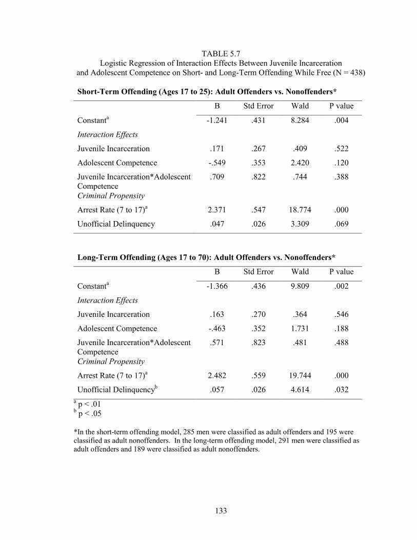
133
TABLE 5.7 Logistic Regression of Interaction Effects Between Juvenile Incarceration
and Adolescent Competence on Short- and Long-Term Offending While Free (N = 438) Short-Term Offending (Ages 17 to 25): Adult Offenders vs. Nonoffenders*
B Std Error Wald P value Constanta -1.241 .431 8.284 .004 Interaction Effects Juvenile Incarceration .171 .267 .409 .522 Adolescent Competence -.549 .353 2.420 .120 Juvenile Incarceration*Adolescent Competence
.709 .822 .744 .388
Criminal Propensity Arrest Rate (7 to 17)a 2.371 .547 18.774 .000 Unofficial Delinquency .047 .026 3.309 .069
Long-Term Offending (Ages 17 to 70): Adult Offenders vs. Nonoffenders* B Std Error Wald P value
Constanta -1.366 .436 9.809 .002 Interaction Effects Juvenile Incarceration .163 .270 .364 .546 Adolescent Competence -.463 .352 1.731 .188 Juvenile Incarceration*Adolescent Competence
.571 .823 .481 .488
Criminal Propensity Arrest Rate (7 to 17)a 2.482 .559 19.744 .000 Unofficial Delinquencyb .057 .026 4.614 .032
a p < .01 b p < .05
*In the short-term offending model, 285 men were classified as adult offenders and 195 were classified as adult nonoffenders. In the long-term offending model, 291 men were classified as adult offenders and 189 were classified as adult nonoffenders.

FIGURE 3.1Actual Mean Number of Offenses for Total Crime: Ages 17 to 70
0
0.1
0.2
0.3
0.4
0.5
0.6
0.7
0.8
0.9
1
17 19 21 23 25 27 29 31 33 35 37 39 41 43 45 47 49 51 53 55 57 59 61 63 65 67 69Age
Mean
numb
er of
offens
es

FIGURE 4.1Offending Trajectories* of Total Crime, Ages 25 to 32 (N = 480)
0
1
2
3
4
5
6
7
25 26 27 28 29 30 31Age
Offen
ding
High-level Declining Offenders (5.9%)Low-level Declining Offenders (10.9%)Inclining Offenders (6.6%)Low-level Offenders (28.7%)Nonoffenders (47.9%)
* The offending trajectories in this model represent the mean number of arrests per year free for all ages.

FIGURE 4.2Impact of Binding Life Event Scale Score (Age 17 to 25) on Short-Term Offending Trajectory
Group Probabilities (Age 25 to 32)*
0.000
0.100
0.200
0.300
0.400
0.500
0.600
0.700
0.800
0.900
1 3 5 7 9Binding Life Event Scale Score
Probab
ility
High-level Declining Offenders (N = 27)Inclining Offenders or Low-Level Declining Offenders (N = 77)Nonoffenders or Low-Level Offenders (N = 376)
* The predicted probabilities are calculated with the control variables set at their mean values.

FIGURE 4.3Offending Trajectories* of Total Crime, Ages 32 to 45 (N = 480)
0
0.5
1
1.5
2
2.5
3
32 33 34 35 36 37 38 39 40 41 42 43 44Age
Offen
ding High-level Offenders (3.2%)
Mid-level Offenders (15.0%)Low-level Offenders (33.1%)Nonoffenders (48.7%)
* The offending trajectories in this model represent the mean number of arrests per year for all ages. These do not take incarceration into account.

FIGURE 4.4Offending Trajectories* for Total Crime, Ages 25 to 70 (N = 480)
0
0.5
1
1.5
2
2.5
3
25 27 29 31 33 35 37 39 41 43 45 47 49 51 53 55 57 59 61 63 65 67 69
Age
Offen
ding
High-level Late Declining Offenders (3.3%)High-level Declining Offenders (16.3%)Low-level Declining Offenders (27.4%)Nonoffenders (53.0%)
* The offending trajectories in this model represent the mean number of arrests per year free for ages 25 to 32 but do not take incarceration into accountfor ages 32 to 70.

FIGURE 4.5Impact of Binding Life Event Scale Score (Age 17 to 25) on Long-Term Offending Trajectory
Group Probabilities (Age 25 to 70)*
0.000
0.050
0.100
0.150
0.200
0.250
0.300
0.350
0.400
0.450
0.500
1 3 5 7 9Binding Life Event Scale
Probab
ility
Nonoffenders (N = 269)Low-level Declining Offenders (N = 120)High-level Declining Offenders (N = 76)High-level Late Declining Offenders (N = 15)
* The predicted probabilities are calculated with the control variables set at their mean values.

FIGURE 4.6Offending Trajectories* for Total Crime, Ages 32 to 70 (N = 480)
0
0.5
1
1.5
2
2.5
3
3.5
4
32 33 34 35 36 37 38 39 40 41 42 43 44 45 46 47 48 49 50 51 52 53 54 55 56 57 58 59 60 61 62 63 64 65 66 67 68 69Age
Offen
ding
High-level Late Declining Offenders (2.2%)High-level Declining Offenders (2.4%)Low-level Declining Offenders I (15.9%)Low-level Declining Offenders II (31.7%)Nonoffenders (47.7%)
* The offending trajectories in this model represent the mean number of arrests per year for all ages. These do not take incarceration into account.

FIGURE 5.1Offending Trajectories* of Total Crime, Ages 17 to 25 (N = 480)
0
0.5
1
1.5
2
2.5
3
3.5
4
4.5
17 18 19 20 21 22 23 24Age
Offen
ding
High-level Declining Offenders (18.5%)Low-level Declining Offenders (22.7%)Inclining Offenders (19.0%)Nonoffenders (39.8%)
* The offending trajectories in this model represent the mean number of arrests per year free for all ages.

FIGURE 5.2Offending Trajectories* for Total Crime, Ages 17 to 70 (N = 480)
0
0.5
1
1.5
2
2.5
17 19 21 23 25 27 29 31 33 35 37 39 41 43 45 47 49 51 53 55 57 59 61 63 65 67 69Age
Offen
ding
High-level Late Declining Offenders (3.9%)High-level Declining Offenders (25.5%)Low-Level Declining Offenders (32.2%)Nonoffenders (38.5%)
* The offending trajectories in this model represent the mean number of arrests per year free for ages 17 to 32. These do not take incarceration into account forages 32 to 70.

143
REFERENCES Abbott, Andrew. 1997. “On the Concept of Turning Point.” Comparative Social
Research 16: 85-105.
Akers, Ronald L. 1991. “Self-Control as a General Theory of Crime.” Journal of
Quantitative Criminology 7: 201-211.
Bazemore, Gordon. 2000. “Community Justice and a Vision of Collective Efficacy: The
Case of Restorative Conferencing.” Pp. 225-297 in Criminal Justice 2000, Volume 3:
Policies, Processes, and Decisions of the Criminal Justice System, ed. Julie Horney.
Washington, DC: U.S. Department of Justice.
Blumstein, Alfred, Jacqueline Cohen, Jeffrey Roth, and Christy Visher, eds. 1986.
Criminal Careers and Career Criminals. Washington, D.C.: National Academy Press.
Bouffard, Leana Allen and John H. Laub. 2004. “Jail or the Army: Does Military
Service Facilitate Desistance?" Pp. 129-151 in After Crime and Punishment, ed. Shadd
Maruna and Ross Immarigeon. London: Willan Publishing.
Braithwaite, John. 1989. Crime, Shame, and Reintegration. Cambridge: Cambridge
University Press.
Braman, Donald. 2002. "Families and Incarceration." Pp. 117-135 in Invisible
Punishment: The Collateral Consequences of Mass Imprisonment, eds. Marc Mauer
and Meda Chesney-Lind. New York: The New Press.
Bushway, Shawn D., Robert Brame, and Raymond Paternoster. 1999. “Assessing
Stability and Change in Criminal Offending: A Comparison of Random Effects,
Semiparametric, and Fixed Effects Modeling Strategies.” Journal of Quantitative
Criminology 15: 23-61.

144
Bushway, Shawn D., Alex R. Piquero, Lisa M. Broidy, Elizabeth Cauffman, and Paul
Mazerolle. 2001. “An Empirical Framework for Studying Desistance as a Process.”
Criminology 39: 491-515.
Caspi, Avshalom, and Terrie E. Moffitt. 1993. “When Do Individual Differences Matter?
A Paradoxical Theory of Personality Coherence.” Psychological Inquiry 4: 247-271.
Clausen, John A. 1991. “Adolescent Competence and the Shaping of the Life Course.”
American Journal of Sociology 96: 805-842.
------ 1993. American Lives: Looking Back at the Children of the Great Depression. New
York: Free Press.
Coleman, James S. 1988. ‘Social Capital in the Creation of Human Capital.” American
Journal of Sociology 94: S95-S120.
Conley, James J. 1985. “Longitudinal Stability of Personality Traits: A Multitrait-
Multimethod-Multioccassion Analysis.” Journal of Personality and Social Psychology
49: 1266-1282.
Dannefer, Dale. 1984. “Adult Development and Social Theory: A Paradigmatic
Reappraisal.” American Sociological Review 49: 100-116.
------. 1987. “Aging as Intracohort Differentiation: Accentuation, the Matthew Effect, and
the Life Course.” Sociological Forum 2: 211-236.
------. 2003. “Cumulative Advantage/Disadvantage and the Life Course: Cross-
Fertilizing Age and Social Science Theory.” Journal of Gerontology 58B: S327-S337.
D’Unger, Amy V., Kenneth C. Land, Patricia L. McCall, and Daniel S. Nagin. 1998.
“How Many Latent Classes of Delinquent/Criminal Careers? Results from Mixed
Poisson Regression Analyses.” American Journal of Sociology 103: 1593-1630.

145
Durkheim, Emile. (1897) 1951. Suicide: A Study in Sociology, translated by John A.
Spaulding and George Simpson. Glencoe, Ill.: Free Press.
Eccles, Jacquelynne S. and Jennifer Appleton Gootman (eds.). 2002. Community
Programs to Promote Youth Development. Washington, D.C.: National Academy
Press.
Elder, Glen H., Jr. 1985. "Perspectives on the Life Course." Pp. 23-49 in Life Course
Dynamics, ed. Glen H. Elder, Jr. Ithaca: Cornell University Press.
------. 1986. “Military Times and Turning Points in Men's Lives.” Developmental
Psychology 22: 233-245.
Eggleston, Elaine, John H. Laub, and Robert J. Sampson. 2004. “Methodological
Sensitivities to Latent Class Analysis of Long-Term Criminal Trajectories.” Journal of
Quantitative Criminology 20: 1-26.
Evans, T. David, Francis T. Cullen, Velmer S. Burton, Jr., R. Gregory Dunaway, and
Michael L Benson. 1997. “The Social Consequences of Self-Control: Testing the
General Theory of Crime.” Criminology 35: 475 – 504.
Farrington, David P. 1983. “Offending from 10 to 25 years of age.” Pp. 17 - 37 in
Prospective Studies of Crime and Delinquency, ed. Katherine Teilmann Van Dusen and
Sarnoff A. Mednick. Boston: Kluwer-Nijhoff Publishing.
Farrington, David P., and Rolf Loeber. 2000. “Some Benefits of Dichotomization in
Psychiatric and Criminological Research.” Criminal Behaviour and Mental Health 10:
100-122.
Farrington, David P., and Donald J. West. 1995. “Effects of Marriage, Separation, and
Children on Offending by Adult Males.” Pp. 249-281 in Current Perspectives on Aging

146
and the Life Cycle, Volume 4: Delinquency and Disrepute in the Life Course, ed. Zena
Smith Blau and John Hagan. Greenwich, Conn.: JAI Press, Inc.
Farrington, David P., Bernard Gallagher, Lynda Morley, Raymond J. St. Ledger, and
Donald J. West. 1986. “Unemployment, School Leaving, and Crime.” British Journal
of Criminology 26: 335-356.
Frederick, Shane, George Loewenstein, and Ted O’Donoghue. 2002. “Time Discounting
and Time Preference: A Critical Review.” Journal of Economic Literature 40: 351-
401.
Giordano, Peggy C., Stephen A. Cernkovich, and Jennifer L. Rudolph. 2002. “Gender,
Crime, and Desistance: Toward a Theory of Cognitive Transformation.” American
Journal of Sociology 107: 990-1064.
Glaser, Daniel. 1969. The Effectiveness of a Prison and Parole System, abridged ed.
Indianapolis, Ind.: Bobbs-Merrill.
Glueck, Sheldon, and Eleanor Glueck. 1930. 500 Criminal Careers. New York: A.A.
Knopf.
------ 1940. Juvenile Delinquents Grown Up. New York: The Commonwealth Fund.
------ 1943. Criminal Careers in Retrospect. New York: The Commonwealth Fund.
------ 1950. Unraveling Juvenile Delinquency. New York: The Commonwealth Fund.
------ 1968. Delinquents and Nondelinquents in Perspective. Cambridge, Mass.: Harvard
University Press.
Goffman, Erving. 1961. Asylums: Essays on the Social Situation of Mental Patients and
Other Inmates. Garden City, NY: Anchor Books.
Gordis, Leon. 1996. Epidemiology. Philadelphia: W.B. Saunders Company.

147
Gottfredson, Michael R., and Travis Hirschi. 1990. A General Theory of Crime. Stanford,
Calif.: Stanford University Press.
Grasmick, Harold G., Charles R. Tittle, Robert J. Bursik, Jr., and Bruce J. Arneklev.
1993. "Testing the Core Empirical Implications of Gottfredson and Hirschi's General
Theory of Crime." Journal of Research in Crime and Delinquency 30: 5-29.
Hagan, John. 1998. “Life Course Capitalization and Adolescent Behavioral
Development.” Pp. 499-517 in New Perspectives on Adolescent Risk Behavior, ed.
Richard Jessor. Cambridge, Cambridge University Press.
Harrison, Paige M., and Allen J. Beck. 2004. Prisoners in 2003. Washington, DC: US.
Department of Justice.
Harrison, Paige M., and Jennifer C. Karberg. 2004. Prison and Jail Inmates at Midyear
2003. Washington, DC: US. Department of Justice.
Hawkins, J. David, Todd I. Herrenkohl, David P. Farrington, Devon Brewer, Richard F.
Catalano, and Tracy W. Harachi. 1998. “A Review of Predictors of Youth Violence.”
Pp. 106-146 in Serious and Violent Juvenile Offenders: Risk Factors and Successful
Interventions, ed. Rolf Loeber and David P. Farrington. Thousand Oaks, Calif.: Sage
Publications.
Hirschi, Travis. 1969. Causes of Delinquency. Berkeley: University of California Press.
Hogan, Dennis P. 1978. “The Variable Order of Events in the Life Course.” American
Sociological Review 43: 573-586.
------. 1980. “The Transition to Adulthood as a Career Contingency.” American
Sociological Review 45: 261-276.

148
Horney, Julie, D. Wayne Osgood, and Ineke Haen Marshall. 1995. “Criminal Careers in
the Short-Term: Intra-Individual Variability in Crime and Its Relation to Local Life
Circumstances.” American Sociological Review 60: 655-673.
House, James S., Debra Umberson, and Karl R. Landis. 1988. “Structures and Processes
of Social Support.” Annual Review of Sociology 14: 293-318.
Irwin, John. 1970. The Felon. Englewood Cliffs, NJ: Prentice-Hall.
Jaccard, James, Robert Turrisi, and Choi K. Wan. 1990. Interaction Effects in Multiple
Regression. Newbury Park, Calif.: Sage Publications.
Knight, B.J., S.G. Osborn, and D.J. West. 1977. “Early Marriage and Criminal Tendency
in Males.” British Journal of Criminology 17: 348-360.
Laub, John H. 2002. “Introduction: The Life and Work of Travis Hirschi.” Pp. xi-xlix in
The Craft of Criminology: Selected Papers by Travis Hirschi. New Brunswick, N.J.:
Transaction Books.
Laub, John H., and Leana C. Allen. 2000. “Life Course Criminology and Community
Corrections.” Perspectives 24: 20-29.
Laub, John H., Daniel S. Nagin, and Robert J. Sampson. 1998. “Trajectories of Change in
Criminal Offending: Good Marriages and the Desistance Process.” American
Sociological Review 63: 225-238.
Laub, John H., and Robert J. Sampson. 1995. “The Long-Term Effects of Punitive
Discipline.” Pp. 247-258 in Coercion and Punishment in Long-Term Perspectives, ed.
Joan McCord. Cambridge: Cambridge University Press.
------. 1998. “The Long-Term Reach of Adolescent Competence: Socioeconomic
Achievement in the Lives of Disadvantaged Men.” Pp. 89-112 in Competence and

149
Character Through Life, ed. Anne Colby, Jacquelyn James, and Daniel Hart. Chicago:
University of Chicago Press.
------ 2001. “Understanding Desistance from Crime.” Pp. 1-69 in Crime and Justice: A
Review of Research, Volume 28, ed. Michael Tonry. Chicago: University of Chicago
Press.
------ 2003. Shared Beginnings, Divergent Lives: Delinquent Boys to Age 70.
Cambridge, Mass.: Harvard University Press.
Liao, Tim Futing. 1994. Interpreting Probability Models: Logit, Probit, and Other
Generalized Linear Models. Thousand Oaks, Calif.: Sage Publications.
Longshore, Douglas, Susan Turner, and Judith A. Stein. 1996. "Self-Control in a
Criminal Sample: An Examination of Construct Validity." Criminology 34: 209-227.
Marcus, Bernd. 2004. "Self-Control in the General Theory of Crime: Theoretical
Implications of a Measurement Problem." Theoretical Criminology 8: 33-55.
Masten, Ann S., and J. Douglas Coatsworth. 1998. “The Development of Competence in
Favorable and Unfavorable Environments: Lessons from Research on Successful
Children.” American Psychologist 53: 205-220.
Mattick, Hans W. 1960. “Parolees in the Army During World War II.” Federal Probation
24: 49-55.
Meisenhelder, Thomas. 1977. “An Exploratory Study of Exiting from Criminal
Careers.” Criminology 15: 319-334.
Merton, Robert. 1968. “The Matthew Effect in Science.” Science 159: 56-63.

150
Moss, Howard A., and Elizabeth J. Susman. 1980. “Longitudinal Study of Personality
Development.” Pp. 530-595 in Constancy and Change in Human Development, ed.
Orville G. Brim, Jr. and Jerome Kagan. Cambridge, Mass: Harvard University Press.
Nagin, Daniel S. 1999. “Analyzing Developmental Trajectories: A Semi-Parametric,
Group-Based Approach.” Psychological Methods 4: 139-157.
------. 2005. Group-Based Modeling of Development over the Life Course. Cambridge,
Mass: Harvard University Press.
Park, Nansook. 2004. “The Role of Subjective Well-Being in Positive Youth
Development” Annals of the American Academy of Political and Social Sciences
591:25-39.
Paternoster, Raymond, Charles W. Dean, Alex Piquero, Paul Mazerolle, and Robert
Brame. 1997. “Generality, Continuity, and Change in Offending.” Journal of
Quantitative Criminology 13:231-266.
Piquero, Alex R., Alfred Blumstein, Robert Brame, Rudy Haapanen, Edward P. Mulvey,
and Daniel S. Nagin. 2001. “Assessing the Impact of Exposure Time and
Incapacitation on Longitudinal Trajectories of Criminal Offending.” Journal of
Adolescent Research 16: 54-74.
Pratt, Travis C. and Frank T. Cullen. 2000. "The Empirical Status of Gottfredson and
Hirschi's General Theory of Crime: A Meta-Analysis." Criminology 38: 931-964.
Rand, Alicia. 1987. “Transitional Life Events and Desistance from Delinquency and
Crime.” Pp. 134-162 in From Boy to Man, From Delinquency to Crime, ed. Marvin E.
Wolfgang, Terence P. Thornberry, and Robert Figlio. Chicago: University of Chicago
Press.

151
Raudenbush, Stephen W., and Anthony S. Bryk. 2002. Hierarchical Linear Models:
Applications and Data Analysis Methods, Second Edition. Thousand Oaks, Calif.:
Sage.
Raudenbush, Stephen W., Anthony S. Bryk, and Richard Congdon. 2004. HLM6:
Hierarchical Linear and Nonlinear Modeling. Lincolnwood, IL: Scientific Software
International.
Reiss, Albert J., Jr. 1989. “Ending Criminal Careers.” Prepared for the Final Report of the
“Desistance/Persistence Working Group” of the Program on Human Development and
Criminal Behavior. MacArthur Foundation and National Institute of Justice.
Reitzes, Dietrich. 1955. The Effects of Social Environment upon Former Felons.”
Journal of Criminal Law, Criminology, and Police Science 46: 226-231.
Rindfuss, Ronald R., C. Gary Swicegood, and Rachel A. Rosenfeld. 1987. “Disorder in
the Life Course: How Common and Does it Matter?” American Sociological Review
52: 785-801.
Rose, Dina R., and Todd R. Clear. 1998. “Incarceration, Social Capital, and Crime:
Implications for Social Disorganization Theory.” Criminology 36: 441-479.
Ross, Catherine E., and Chia-Ling Wu. 1996. “Education, Age, and the Cumulative
Advantage in Health.” Journal of Health and Social Behavior 37: 104-120.
Rutter, Michael. 1979. “Protective Factors in Children’s Responses to Stress and
Disadvantage.” Pp. 49-74 in Primary Prevention of Psychopathology, Volume 3:
Social Competence in Children, ed. Martha Whalen Kent, and Jon E. Rolf. Hanover,
NH: University Press of New England.

152
------. 1985. “Resilience in the Face of Adversity: Protective Factors and Resistance to
Psychiatric Disorder.” British Journal of Psychiatry 147: 598-611.
------. 1987. “Psychosocial Resilience and Protective Mechanisms.” American Journal of
Orthopsychiatry 57: 316-331.
------. 1990. “Psychosocial Resilience and Protective Mechanisms.” Pp. 181-214 in Risk
and Protective Factors in the Development of Psychopathology, ed. Jon Rolf, Ann S.
Masten, Dante Cicchetti, Keith H. Nuechterlein, and Sheldon Weintraub. Cambridge:
Cambridge University Press.
------. 1994a. “Beyond Longitudinal Data: Causes, Consequences, Changes, and
Continuity.” Journal of Consulting and Clinical Psychology 62: 928-940.
-------. 1994b. “Continuities, Transitions and Turning Points in Development." Pp. 1-25
in Development Through Life, ed. M. Rutter and D.F. Hay. Oxford: Blackwell
Scientific Publications.
-------. 1996. “Transitions and Turning Points in Developmental Psychopathology: As
Applied to the Age Span Between Childhood and Mid-Adulthood.” International
Journal of Behavioral Development 19: 603-626.
Rutter, Michael, Henri Giller, and Ann Hagell. 1998. Antisocial Behavior by Young
People. Cambridge: Cambridge University Press.
Sampson, Robert J., and John H. Laub. 1990. “Crime and Deviance Over the Life
Course: The Salience of Adult Social Bonds.” American Sociological Review, 55: 609-
627.
------. 1992. "Crime and Deviance in the Life Course." Annual Review of Sociology: 18:
63-84.

153
------. 1993. Crime in the Making: Pathways and Turning Points Through Life.
Cambridge, Mass.: Harvard University Press.
------. 1996. “Socioeconomic Achievement in the Life Course of Disadvantaged Men:
Military Service as a Turning Point, Circa 1940-1965.” American Sociological Review
61: 347-367.
------. 1997. “A Life-Course Theory of Cumulative Disadvantage and the Stability of
Delinquency.” Pp. 133-161 in Developmental Theories of Crime and Delinquency, ed.
Terence P. Thornberry. New Brunswick, N.J.: Transaction Publishers.
Sampson, Robert J., John H. Laub, and Elaine P. Eggleston. 2004. “The Aftermath of
Incarceration in the Lives of Disadvantaged Men: A 50-Year Follow-Up Study.” Final
Report prepared for “The ‘Mass’ Incarceration Working Group.” New York: Russell
Sage Foundation.
Shanahan, Michael J. 2000. “Pathways to Adulthood in Changing Societies: Variability
and Mechanisms in Life Course Perspective.” Annual Review of Sociology 26: 667-
692.
Shover, Neal. 1996. Great Pretenders: Pursuits and Careers of Persistent Thieves.
Boulder, Colo.: Westview Press.
Sykes, Gresham M. 1958. The Society of Captives: A Study of Maximum Security Prison.
Princeton, N.J.: Princeton University Press.
Tittle, Charles R., David A. Ward, and Harold G. Grasmick. 2003. “Self-Control and
Crime/Deviance: Cognitive vs. Behavioral Measures.” Journal of Quantitative
Criminology 19: 333-365.

154
Tracy, Paul E. and Kimberly Kempf-Leonard. 1996. Continuity and Discontinuity in
Criminal Careers. New York: Plenum Press.
Uggen, Christopher. 2000. “Work as a Turning Point in the Life Course of Criminals: A
Duration Model of Age, Employment, and Recidivism.” American Sociological Review
65: 529-546.
Umberson, Debra. 1987. “Family Status and Health Behaviors: Social Control as a
Dimension of Social Integration.” Journal of Health and Social Behavior 28: 306-319.
U.S. Department of Justice, Bureau of Justice Statistics. 1993. National Corrections
Reporting Program: [United States] [Computer File]. Conducted by U.S. Department
of Commerce, Bureau of the Census. ICPSR ed. Ann Arbor, MI: Inter-university
Consortium for Political and Social Research [producer and distributor], 1997.
Warr, Mark. 1998. “Life-Course Transitions and Desistance From Crime.” Criminology
36: 183-216.
Werner, Emmy E. and Ruth S. Smith. 1992. Overcoming the Odds: High Risk Children
from Birth to Adulthood. Ithaca, New York: Cornell University Press.
Western, Bruce, and Katherine Beckett. 1999. “How Unregulated is the U.S. Labor
Market? The Penal System as a Labor Market Institution.” American Journal of
Sociology 104: 1030-1060.
Wolfgang, Marvin E., Terence P. Thornberry, and Robert Figlio, eds. 1987. From Boy to
Man, From Delinquency to Crime. Chicago: University of Chicago Press.
Wright, Bradley R. Entner, Avshalom Caspi, Terrie E. Moffitt, and Phil A. Silva. 1999.
“Low Self-Control, Social Bonds, and Crime: Social Causation, Social Selection, or
Both?” Criminology 37: 479-514.

155
------. 2001. “The Effects of Social Ties on Crime Vary by Criminal Propensity: A Life-
Course Model of Interdependence.” Criminology 39: 321-351.