Alternative Models for Stock Price Dynamics1

Mikhail Chernov

Columbia University

A. Ronald Gallant

University of North Carolina

Eric Ghysels

University of North Carolina

George Tauchen

Duke University

First draft: September 2000

Last revised: January 23, 2001

1A preliminary draft of the paper was presented at the CAP Mathematical Finance Workshop,

Columbia University, the Conference on Risk Neutral and Objective Probability Distributions,

Fuqua School of Business, Duke University and at Vanderbilt University. We would like to thank the

conference and seminar pariticpants, as well as Luca Benzoni, Paul Glasserman, Michael Johannes

and Nour Meddahi, for their comments.

Abstract

The purpose of this paper is to shed further light on the tensions that exist between the empirical �t

of stochastic volatility (SV) models and their linkage to option pricing. A number of recent papers

have investigated several speci�cations of one-factor SV di�usion models associated with option

pricing models. The empirical failure of one-factor aÆne, Constant Elasticity of Variance (CEV),

and one-factor logarithmic SV models leaves us with two strategies to explore: (1) add a jump

component to better �t the tail behavior or (2) add an additional (continuous path) factor where

one factor controls the persistence in volatility and the second determines the tail behavior. Both

have been partially pursued and our paper embarks on a more comprehensive examination which

yields some rather surprising results. Adding a jump component to the basic Heston aÆne model is

known to be a successful strategy as demonstrated by Andersen et al. (1999), Eraker et al. (1999),

Chernov et al. (1999), and Pan (1999). Unfortunately, the presence of a jump component introduces

quite a few unpleasant econometric issues. In addition, several �nancial issues, like hedging and

risk factors become more complex. In this paper we show that a two-factor logarithmic SV di�usion

model (without jumps) appears to yield a remarkably good empirical �t. We estimate the model

via the EMM procedure of Gallant and Tauchen (1996) which allows us to compare the non-nested

logarithmic SV di�usion with the aÆne jump speci�cation. Obviously, there is one drawback to

the logarithmic SV models when it comes to pricing derivatives since no closed-form solutions are

available. Against this cost weights the advantage of avoiding all the complexities involved with

jump processes.

JEL classi�cation: G13; C14, C52, C53

Key Words: EÆcient method of moments, Poisson jump processes, Stochastic volatility models

1

Introduction

The purpose of this paper is to shed further light on the tensions which exist between the

empirical �t of stochastic volatility (SV) models and their linkage to option pricing. While SV

models are well-established, there are still many unresolved questions about the empirical

merits and shortcomings of the available speci�cations. A number of recent papers have

investigated the Heston (1993) option pricing SV model. It is a natural starting point since

it is the simplest among the class of aÆne di�usion models. It implies that the stock-price

process follows a geometric Brownian motion with stochastic variance governed by a square-

root mean-reverting process. Using di�erent estimation techniques and/or sample data,

Andersen et al. (1999), Benzoni (1998), Chernov and Ghysels (2000), Jones (2000), Eraker

et al. (1999) and Pan (1999) reject the model resoundingly because it is not able to generate

enough kurtosis. Jones (2000) estimates an SV model with CEV volatility dynamics, which

unlike the aÆne di�usion, features state-dependent volatility of volatility. Unfortunately,

contrary to the Heston model, the CEV model generates too many extreme observations.

Andersen et al. (2000) compare the empirical �t of the Scott (logarithmic volatility) and

Heston models using returns data and conclude that neither model is accepted and are

roughly equivalent in empirical (mis)�t. Moreover, Benzoni (1998) also �nds that these

models are roughly the same in terms of option (mis)pricing.

These observations prompt us to embark on a comprehensive examination of models with

two stochastic volatility factors. The presence of two volatility factors breaks the link between

tail thickness and volatility persistence i.e. one factor controls persistence while another

handles kurtosis. The analysis is structured as a comparison of three types of two-factor

models, they are (1) logarithmic di�usions with two continuous path volatility factors, (2)

aÆne di�usions with two continuous path factors and (3) aÆne di�usions with a mixture of

continuous path volatility factor and a discrete jump component. Adding a jump component

to the basic Heston aÆne model turns out to be a successful strategy as demonstrated by

Andersen et al. (1999), Chernov et al. (1999) and Eraker et al. (1999). Unfortunately, the

presence of a jump component introduces quite a few unpleasant econometric issues. Jump

components are diÆcult to estimate and complicate the extraction of the volatility process,

an issue so far only addressed by Eraker et al. (1999) using MCMC methods. Moreover, the

evidence from options data indicates that jumps are not suÆcient to generate all empirical

regularities in the data, and the stochastic volatility of volatility in particular.1 The results

1See Bakshi, Cao, and Chen (1997), Bates (2000), Jones (2000), Pan (2000) and discussion in the next

section.

2

we �nd show that a two-factor logarithmic SV di�usion model (without jumps) yields a

remarkably good empirical �t, i.e. the model is not rejected at conventional signi�cance

levels unlike the jump di�usion and aÆne two-factor models.2 The fact that logarithmic

volatility factors are used, instead of the aÆne speci�cation, adds the exibility of state

dependent volatility as noted by Jones (2000). In addition an appealing feature of the

logarithmic speci�cation is the multiplicative e�ect of volatility factors on returns. One

volatility factor takes care of long memory, whereas the second factor is fast mean-reversting

(but not a spike like a jump). This property of logarithmic models facilitates mimicking

the very short-lived but erratic extreme event behavior through the second volatility factor.

Neither one volatility factor models with jumps nor aÆne two-factor speci�cations are well

equiped to handle such patterns typically found during �nancial crisis.

Finally, the EMM estimation approach of Gallant and Tauchen (1996) allows for a formal

statistical comparison of the non-nested two-factor logarithmic volatility and aÆne factor

with jump process model speci�cations. Obviously, there is one drawback to logarithmic SV

di�usion models when it comes to pricing derivatives. Unlike the aÆne di�usions with jumps,

no closed-form solutions are readily available and pricing formulas need to be mimicked by

simulation. While a drawback it may also serve as an advantage with respect to risk-neutral

measure transformations. Moreover, adopting a logarithmic volatility speci�cation avoids all

the complexities involved with jump processes which need to be added to aÆne di�usions.

The paper is organized as follows. In a �rst section we describe the SV models that we

consider in the study. The next section covers the estimation methods, brie y summarizing

EMM procedure and the SNP model selection. Section three reports the empirical results.

A �nal section concludes the paper.

1 Continuous time SV Models

In recent years we have made considerable progress on various aspects of estimating di�usions

particularly those involving stochastic volatility or other latent factors. The literature on the

estimation of di�usions with or without stochastic volatility and/or jumps, is summarized in

a number of surveys and textbooks, including Bates (1996), Campbell et al. (1996), Ghysels

et al. (1996), Melino (1994), Renault (1997) and Tauchen (1997). Research is focusing more

2We are not the �rst to suggest two-factor logarithmic SV models, see for instance Alizadeh et al. (1999),

Chacko and Viceira (1999), Gallant, Hsu and Tauchen (1999) and the two-factor GARCH model of Engle

and Lee (1999).

3

on model speci�cation and diagnostics, now that estimation procedures are �ne-tuned and

more widely available. It is natural that attention went �rst to the stochastic volatility

models known from the option pricing literature, in particular the models of Heston (1993)

and Hull and White (1987). Unfortunately, we have come to a consensus that neither model

is capable of generating the tail behavior and volatility dynamics observed in equity index

data such as the S&P 500 series. These conclusions can be drawn from several papers,

including Andersen et al. (1999), Benzoni (1998), Chernov and Ghysels (2000), Eraker et al.

(1999), Jones (2000) and Pan (1999).

This consensus is the starting point of our paper. We consider models with at most four

factors, namely:

dPt=Pt = (�10 + �12U2t) dt+ � (U3t; U4t) (dW1t + 13dW3t + 14dW4t) (1)

dU2t = (�20 + �22U2t) dt+ �20dW2t (2)

In the above, Pt represents the �nancial price series evolving in continuous time (we reserve

the notation U1t for the logarithm of the price). We allow for a exible drift speci�cation

via a stochastic factor U2t; which evolves according to the Ornstein-Uhlenbeck process. This

speci�cation can accommodate the mild serial correlation appearing in the returns series,

which may be explained by the nonsynchronous trading and unexpected stochastic dividend

e�ects. An alternative strategy to incorporate these e�ects would be to pre�lter the data as

was done in Andersen et al. (1999) or Gallant et al. (1993). We model the di�usion coeÆcient

� as a function of two stochastic volatility factors U3t and U4t. We will use both aÆne and

logarithmic speci�cations for these two factors. Finally, 13 and 14 capture the leverage

e�ect. While we assume the usual probability space setup for (1) we will not assume the

usual regularity conditions for the logarithmic speci�cations. This will be discussed later

and also in Appendix A.

This speci�cation yields the classical models of Heston (1993) and Scott (1987) when U2t

and U4t are switched o�. These models proved to be a substantial improvement over the

Black-Scholes speci�cation because of their formulation of volatility as a random persistent

process. However, this persistence turned out to be the weakness of the model as well:

the EMM estimation diagnostics reported by for instance Andersen et al. (1999) (and also

discussed in the next sections) show that the main diÆculty is that the speci�cations do

not generate enough tail thickness in the implied transition density of the returns series. In

other words, extreme movements in returns occur more frequently in the observed data than

would be implied by the Heston or Scott model dynamics.

A common generalization is to augment the price dynamics in the one-factor SV version

4

of (1) with a jump component described by a Poisson process. The continuous path stochas-

tic volatility part accommodates the persistence in the returns volatility whereas the discrete

jump component accommodates the infrequent large price movements and hence accommo-

dates the tail behavior. These models have received considerable attention recently. Various

papers have examined the econometric estimation and/or derivative security pricing with

such processes. Examples include Bates (1996a), Ho, Perraudin and S�rensen (1996), Scott

(1997), Bakshi, Cao and Chen (1997), Scott (1997), Bates (1998), Andersen, Benzoni and

Lund (1999), Chernov et al. (1999) and Pan (1999) among others. Bakshi and Madan (2000)

and DuÆe, Pan and Singleton (2000) provide very elegant general discussions of the class of

aÆne jump-di�usions with stochastic volatility which yield analytic solutions to derivative

security pricing.

However, the evidence from option markets shows that the jump component is not suÆ-

cient to fully capture the dynamics of �nancial series. In particular, Bakshi, Cao and Chen

(1997) and Bates (2000) �nd that the volatility of volatility coeÆcient, which is estimated

from the underlying asset time series is much lower than the one estimated from the options

cross-section. Moreover, Pan (2000) in a study of a joint dataset �nds evidence suggesting

that the volatility of volatility is stochastic. This observation is con�rmed by Jones (2000)

who �nds, based on the implied volatility series, that volatility of volatility is higher during

the more volatile periods in the stock market.

These observations prompt us to explore alternative strategies for generalizing the Heston

and Scott models to better accommodate the data. Speci�cally, we introduce a second

stochastic volatility factor, and we consider more complicated volatility dynamics. These

strategies provide considerable exibility. The presence of two volatility factor breaks the

link between tail thickness and volatility persistence. In models with only a single volatility

factor, these two features get intertwined, since the single factor has to account for both

thick tails and volatility persistence, which proves impossible. This intertwinement has been

noted before in the discrete-time GARCH literature, see e.g. the discussion in Engle and

Lee (1999). By allowing for two factors, we permit one factor to generate tail thickness and

the other to account for volatility persistence. We will introduce the speci�cs of our models

in the following two subsection.

1.1 AÆne Models

AÆne di�usion models are characterized by drift and variance functions which are linear

functions of the factors. Dai, Liu and Singleton (1998) discuss the most general speci�cation

5

of such models including the identi�cation and admissibility conditions. We consider a very

simple representative of this class:

� (U3t; U4t) =q�10 + �13U3t + �14U4t (3)

dUit = (�i0 + �iiUit) dt+q�i0 + �iiUitdWit; i = 3; 4 (4)

The volatility factors enter additively into the di�usion component speci�cation, as in Engle

and Lee (1999). Hence, they could be interpreted as short and long memory components.

The long memory (persistent) component should be responsible for the main part of the

returns distribution, while the short memory component will accommodate the extreme

observations.

Also, as a benchmark, we will consider a zero-mean constant intensity jump di�usion

model of Andersen et al. (2000). Namely we specify the jump component as

dqt = JtdNt; where (5)

dNt � Poi (�Jdt)

Jt � N(0; �2J)

and add it to the aÆne version of (1) when U4t � 0: Andersen, Benzoni, and Lund (1999)

and Chernov et al. (1999) are the most closely related to the current study since they all

share a common EMM estimation approach. Andersen et al. (1999) examine jump processes

of the type appearing in (5), while Chernov et al. (1999) examine more complex processes

with time-varying jump intensity and other jump size distributions. Both papers document

that jump processes can indeed generate thick-tailed error densities but at the cost of greatly

complicating the estimation. For example, the simulation-based EMM algorithm requires

either pro�ling the estimation as a function of the jump intensity parameter, a procedure

followed here and discussed later, or smoothing locally the discrete jumps, as Andersen et

al. (1999) did. Moreover, the extraction of jumps and volatility via reprojection methods

(see Gallant and Tauchen (1998)) is also challenging.

1.2 Logarithmic Models

In logarithmic models the variance is an exponential function of the factors. We consider

the following models from this class:

� (U3t; U4t) = exp (�10 + �13U3t + �14U4t) (6)

dUit = (�i0 + �iiUit) dt+��i0 + �ii Uit

�dWit; i = 3; 4 (7)

6

We study two di�erent avors of the logarithmic models, depending on the value of the

coeÆcients �ii: When �ii = 0, the volatility factors are described by Ornstein-Uhlenbeck

processes. In this case, the drift and variance of these factors are linear functions and, hence,

the model can be described as logarithmic or log-aÆne to be consistent with the previous

subsection. Whenever, �ii 6= 0 either for i = 3 or 4 we have feedback, a feature which will

turn out to be empirically relevant. The key property is that it permits the volatilities of the

volatility factors, via the terms �33U3t and/or �44U4t; to be high when the volatility factors

themselves are high. These terms are found to be important in Gallant, Hsu, and Tauchen

(1999), and Jones (2000). The variance of the factors is a quadratic function in the feedback

model. Extra care should be taken in de�ning the stochastic integrals and solving the SDEs

associated with logarithmic models, because they violate the standard regularity conditions.

We dedicate Appendix A to these issues.

It is perhaps not so surprising that this model has a good empirical �t. Intuitively, the

second factor not only takes care of the tail behavior, as the jump process does, it also

features dynamics that seem appealing for modeling extreme market conditions. Indeed,

the process can accommodate (mild) persistence in volatility during high volatility days,

and when �44 6= 0 (assuming the second factor determines tail behavior), the volatility of

volatility increases as well. These properties cannot be accomplished by a simple Poisson

jump process, which can accommodate tail behavior but not the dynamics of extreme events.

It should also be noted that a nice feature of the logarithmic speci�cation is the multiplicative

e�ect of U3t and U4t on the volatility of returns. Neither aÆne models nor jump processes

feature separate factors which scale multiplicatively the Brownian motionW1t: This property

of logarithmic models facilitates mimicking the very short-lived but erratic extreme event

behavior through the second volatility factor.

1.3 Normalizations and Model Abbreviations

Some normalizations are needed to achieve identi�cation of the various speci�cations de-

scribed in the previous subsection. In the generic speci�cation (1), (2) the long-run mean of

the drift is simultaneously controlled by �10 and �20; while the volatility of the drift volatility

is controlled by �12 and �20: Therefore, we impose:

�20 = 0; �20 = 1 (8)

By analogy, for the general aÆne model in (3) and (4) we impose the restrictions:

�10 = 0; �30 = 0; �33 = 1; �40 = 0; �44 = 1 (9)

7

Finally, for the logarithmic speci�cation (6) and (7) we set

�30 = 0; �40 = 0; �30 = 1; �40 = 1 (10)

Note, that �10 is not equal to zero here, because it controls the long-run mean of the total

volatility.

It proves convenient to have acronyms for the various models:

AFF2V stands for the AFFine Two Volatility factor model, i.e. the most general model

appearing in (1), (2), (3), and (4). This model augments the previous one with an additional

continuous path factor.

AFF1V means the simplest AFFine One Volatility factor model appearing in (1), (2), (3),

and (4). This model with constant drift corresponds to the Heston model.

AFF1V-J represents the simplest AFFine One Volatility factor model with Jumps ap-

pearing in (1), (2), (3), and (4) in combination with the Poisson process as speci�ed in

(5).

LL2VF is the most general model (1), (2), (6), and (7), where the acronym means Log

Linear, Two Volatility Factors, which feature Feedback via �33 6= 0 and �44 6= 0 from the

volatility factors to their own volatilities.

LL2V is the model meaning Log Linear, Two Volatility Factors without volatility feedback

since �33 = 0 and �44 = 0:

LL1VF means the One Volatility factor version of (1), (2), (6), and (7) with �14 = 0

making the second volatility factor irrelevant.

LL1V means the simplest Log Linear One Volatility factor model with no volatility feed-

back.

The speci�cation LL1V is the speci�cation most commonly estimated in the literature,

though Gallant, Hsu, and Tauchen (1999) explored LL2VF, with only modest success for

explaining IBM daily range data.

The various models are summarized in Table 1. In what follows, � denotes the parameters

of the underlying SDE that is to be estimated. For example, for the largest logarithmic

speci�cation LL2VF the parameter vector is

� = (�10; �12; �22; �33; �44; �10; �13; �14; �33; �44; 13; 14) (11)

8

2 EÆcient Method of Moments

Let fytg1t=�1; yt 2 <M ; be a discrete stationary time series. In this paper, fytg is

100 � [log(Pt) � log(Pt�1)]; where Pt is the daily DJIA. When, as here, fytg comes from

a discretely sampled SDE system, then the SDE speci�cation implicitly determines the den-

sity p(yt�L; : : : ; ytj�) of a contiguous stretch of length L + 1 from fytg; where � 2 <p� is a

vector of unknown parameters of the generic di�usion process (1). The fundamental problem

that blocks straightforward application of standard statistical methods is that an analytic

expression for p(yt�L; : : : ; y0j�) is not available. (see for instance Ait-Sahalia, 2000; Elerianet al. 2000, Durham and Gallant, 2000 for further discussion). However, by using simulation,

an expectation of the form

E�(g) =Z� � �Zg(y�L; : : : ; y0) p(y�L; : : : ; y0j�) dy�L � � �dy0

can be computed for given �: That is, for given �; one can generate a simulation fytgNt=1 fromthe system and put

E�(g) = 1

N

NXt=1

g(yt�L; : : : ; yt);

with N large enough that Monte Carlo error is negligible.

The EMM estimation involves simulating continuous path di�usions which has been

covered extensively in the literature. We rely on a standard Euler discretization scheme.3

The simulations involve a sampling frequency with twenty four steps per trading day. The

trading day was set equal to 1=252; therefore the models parameters have annual scaling.

We use a nonstandard approach to simulate the aÆne di�usions from (1), (2), (3), and

(4).4 Instead of a naive discretization of U3t and U4t, we �rst derive the dynamics of logU3t

and logU4t using the Ito's lemma. Then we apply the Euler scheme to these processes. As is

well known, square-root processes require constraints on the coeÆcients for the processes to

stay positive (e.g. Feller, 1951). Given our normalizations in (9), these constraints translate

into �i0 > 0:5 for i = 3; 4: If we directly simulate the aÆne processes these constraints impose

numerical burdens, as it becomes hard to take numerical derivatives and even simulate for

the borderline cases. When we simulate the log-versions of U3t and U4t; we are not concerned

with the positivity of the processes, so we can let the parameters �i0 change freely. This

3SuÆcient conditions for the Euler scheme convergences appearing in Kloeden and Platen (1995) are

violated by the models from the logarithmic class. However, their suÆcient conditions are too strong. We

discuss weaker conditions in the Appendix A.4We are greatful to Michael Johannes for suggesting this.

9

manipulation improves the stability of the procedure tremendously. Therefore , although

aÆne di�usions satisfy the standard regularity conditions, we might expect, on this basis,

that simulating the log provides some increase in numerical accuracy.

We took the following approach with respect to jump component simulation. We opted

a pro�ling approach, where the EMM objective function is optimized with respect to the

parameters � appearing in (11) and the jump size parameters. Since we focus on a standard

Merton type jump process the size distribution is Gaussian and involves two parameters.

The jump frequency is drawn from a Poisson process, with its intensity parameter �xed and

moved over a grid to appraise the overall �t of the model. The jump process was implemented

by drawing durations between jumps from a exponential distribution. When the durations

fell inside the discretization interval, the size of the jump was attributed time-proportionally

to the hourly observations bracketing the jump event. In practice this scheme is equivalent

to the one in Platen and Rebolledo (1985) and hence achieves the same convergence.

Gallant and Tauchen (1996) propose a minimum chi-squared estimator for � in this situa-

tion, which they termed the eÆcient method of moments (EMM) estimator. Being minimum

chi-squared, the optimized chi-square criterion can be used to test system adequacy. The

moment equations that enter the minimum chi-squared criterion of the EMM estimator are

obtained from the score vector (@=@�) log f(ytjxt�1; �) of an auxiliary model f(ytjxt�1; �)where xt�1 is a lagged state vector. The auxiliary model is termed the score generator.

Gallant and Long (1997) show that if the score generator is the SNP density fK(yjx; �K)described below, then the eÆciency of the EMM estimator can be made as close to that of

maximum likelihood as desired by taking K large enough. The �rst step in computing the

EMM estimator �n is to use the score generator

f(ytjxt�1; �) � 2 � (12)

to summarize the data f~yt; ~xt�1gnt=1 by computing the quasi maximum likelihood estimate

~�n =�2�

argmax1

n

nXt=1

log[f(~ytj~xt�1; �)];

and the corresponding estimate of the information matrix

~In = 1

n

nXt=1

h @@�

log f(~ytj~xt�1; ~�n)ih @@�

log f(~ytj~xt�1; ~�n)i0; (13)

The estimator (13) presumes the score generator (12) provides an adequate statistical approx-

imation to the transition density of the data, so that f(@=@�) log f(~ytj~xt�1; ~�n)g is essentiallyserially uncorrelated. If (12) is not adequate, then one of the more complicated expressions

10

for ~In set forth in Gallant and Tauchen (1996) must be used, although the EMM estimator

is still consistent and asymptotically normal. De�ne

m(�; �) = E�(@

@�log[f(y0jx�1; �)]

)

which is computed by averaging over a long simulation

m(�; �):=

1

N

NXt=1

@

@�log[f(ytjxt�1; �)]: (14)

The EMM estimator is

�n =�2<p�

argminm0

(�; ~�n)(~In)�1m(�; ~�n) (15)

The estimator is consistent and asymptotically normally distributed with asymptotic dis-

tribution given in Gallant and Tauchen (1996). Under the null hypothesis that p(y�L; : : : ; y0j�)is the correct model, n times the minimized value of the objective function is asymptotically

chi-squared on p� � p� degrees of freedom where p� and p� are respectively the lengths of

parameter vectors � and �:

The best choice of a moment function to implement simulated method of moments is the

score of a auxiliary model that closely approximates the system dynamics where the parame-

ter vector of the auxiliary model is evaluated at its quasi maximum likelihood estimate. The

SNP density of Gallant and Tauchen (1989, 1991, 2000), which is derived as a location-scale

transform of an innovation density represented as a Hermite expansion leads to a useful,

general purpose auxiliary model. We give a brief description. Here, yt represents the ob-

served process and, for now, xt�1 = (yt�L; :::; yt�1): We frequently drop the time subscripts

and write y and x generically.

If one expandspp(x; y j �o) in a Hermite series, that is, expands the square root of the

stationary density of the system (1) in a Hermite series, and derives the approximation to

the transition density p(y j x; �o) of the system that corresponds to the truncated expansion,

then one obtains an approximating transition density fK(yt j xt�1) that has the form of a

location-scale transform

y = Rxz + �x (16)

of an innovation zt; where Rx is an upper triangular matrix (see Gallant, Hsieh, and Tauchen,

11

1991).5 The density function of the innovation zt; is

hK(zjx) = [P(z; x)]2�(z)R[P(u; x)]2�(u) du; (17)

where P(z; x) is a polynomial in (z; x) of degree K and �(z) denotes the multivariate normal

density function with dimension M; mean vector zero, and variance-covariance matrix the

identity.

It proves convenient to express the polynomial P(z; x) in a rectangular expansion

P(z; x) =KzXjjj=0

0@ KxXjij=0

aijxi

1A zj; (18)

where K = (Kz; Kx); i and j are multi-indexes, and j � j denotes the degree of an index.

Because [P(z; x)]2= R [P(u; x)]2�(u)du is a homogeneous function of the coeÆcients of the

polynomial P(z; x); P(z; x) can only be determined to within a scalar multiple. To achieve

a unique representation, the constant term a00 of the polynomial P(z; x) is put to one. With

this normalization, hK(zjx) has the interpretation of a series expansion whose leading term

is the normal density �(z) and whose higher order terms induce departures from normality.

The advantage of a rectangular expansion is that it gives the polynomial P(z; x) the

interpretation of a polynomial in z of degree Kz whose coeÆcients are polynomials of degree

Kx in x. This is useful in applications because putting Kx = 0 implies that the innovation

density hK(ztjxt�1) does not depend on xt�1 and is therefore homogeneous. That is, if

Kx = 0 none of the moments of the innovation density hK(zjxt�1) will depend on the past.

Conversely, if Kx > 0; then the shape of the innovation distribution does depend on the

history xt�1 = (yt�L; : : : ; yt�1) of the process fytg1t=�1. In the empirical application we will

compare parameter estimates obtained from homogeneous heterogeneous score speci�cations

for certain model speci�cations.

The location function takes the form of an autoregression �x = b0+PLu

k=1Bkyt�k: Conse-

quently, the density determined by the location-scale transform y = Rz + �x together with

the innovation density hK(zjx) is a Gaussian vector autoregression if Kz = Kx = 0. It

is a semi-parametric autoregression along the lines of Engle and Gonzales-Rivera (1991) if

Kz > 0 and Kx = 0; and is a fully nonparametric nonlinear process if Kz > 0 and Kx > 0:

The two choices of Rx that have given good results in applications are an ARCH-like moving

5Although R does not depend on x in this derivation, it proves advantageous in applications to allow

the scale matrix Rx to depend on x because it reduces the degree Kx required to achieve an adequate

approximation to the transition density p(yjx; �o).

12

average speci�cation and a GARCH-like ARMA speci�cation which are discussed in Gallant

and Tauchen (1997). In summary, Lu; Lg; and Lr determine the location-scale transforma-

tion y = Rxzt + �x and hence determine the nature of the leading term of the expansion.

The number of lags in the location function �x is Lu and the number of lags in the scale

function Rx is Lu+Lr. The number of lags that go into the x part of the polynomial P(z; x)is Lp. The parameters Kz; Kx determine the degree of P(z; x) and hence the nature of the

innovation process fztg.

3 Empirical Results

In a �rst subsection we cover the estimation of the auxiliary model. The second subsection

reports and discusses the EMM estimates. A �nal subsection discusses reprojection of the

factors and their properties.

3.1 Data and Auxiliary Model

The raw data for analysis consist of 11,717 daily observations January 2, 1953, to July 16,

1999, on the (geometric) percent movement

yt = 100 � [log(Pt)� log(Pt�1)] (19)

of the Dow Jones Industrial Average (DJIA), Pt. As noted earlier, we use the raw series and

do not perform any transformation on the raw data which are plotted in Figure 1. The �rst is

to project the data fytg onto an auxiliary model, which here we use the SNP model described

above. We reserve the �rst 47 data points for forming lags leaving 11,670 observations, net.

The tuning parameters Lu; Lg; Lr; Lp; Kz; and Kx are selected by moving upward along an

expansion path using the BIC criterion (Schwarz, 1978),

BIC = sn(~�) + (1=2)(pK=n) log(n);

where the objective function sn(�) is given by

sn(�) = � 1

n

nXt=1

log[fK(~ytj~xt�1; �)]

to guide the search. Models with small values of BIC are preferred.

The expansion path has a tree structure. Rather than examining the full tree, the strategy

is to expand �rst in Lu with Lg = Lr = Lp = Kz = Kx = 0 until BIC turns upward. For

13

ARCH-type speci�cations, we expand Lr with Lg = Lp = Kz = Kx = 0; then expand Kz

with Kx = 0; and lastly Lp and Kx. It is useful to expand in Kz; Lp and Kx at a few

intermediate values of Lr because it sometimes happens that the smallest value of BIC lies

elsewhere within the tree. For GARCH-type speci�cations, the strategy is similar: we put

Lg = Lr = 1; then expand Kz; Lp and Kx as above. We then check Lg = Lr = 2. These

two are the only GARCH-type speci�cations considered, which is consistent with standard

practice among GARCH practitioners. There is the diÆculty that increases in Kx add a

plethora of parameters. We control this by restricting the coeÆcients aij of the Hermite

expansion (18) to be zero when jjj > 2 and jij � 1, which was motivated by inspecting

t-statistics on Hermite coeÆcients of larger models without such restrictions. The net e�ect

of the restrictions is that the Hermite coeÆcients of (18) are state dependent, i.e, dependent

upon x, only up through quadratic terms; the Hermite coeÆcients of zj are constant for

cubics and higher.

The �nal SNP model selected via this procedure has

Lu = 1; Lr = 1; Lg = 1; Lp = 1; Kz = 8; Kx = 1 (20)

This SNP model, preferred under BIC, can be characterized as a GARCH(1,1) with a non-

parametric error density represented as an eigth-degree Hermite expansion where the Hermite

coeÆcients up through quadratic terms are state dependent. The model is akin to the semi-

parametric GARCH of Engle and Gonzales-Rivera, except their nonparametric error density

is represented as a state-independent kernel density. (Unlike SNP, the kernel representation

of the semiparametric GARCH precludes state dependence of the error density, which is

found to be empirically important for this data set.)

For purpose of comparison we also consider an homogeneous score where the state de-

pendence of the Hermite polynomial is not incorporated, namely the tuning parameters are

set to:

Lu = 1; Lr = 1; Lg = 1; Lp = 1; Kz = 8; Kx = 0 (21)

In particular for the one-factor aÆne speci�cation we will use this score for comparing the

parameter estimates obtained from the heterogeneous score (20) and the homogeneous one.

The latter is similar to the score considered by Andersen et al. (1999) with the exception

that the lead term is EGARCH instead of GARCH.

In general we proceeded as follows in the estimation of the models. At �rst we used

the homogeneous score (21) to attain a �rst set of parameter estimates and then further

optimized with the heterogenous score. In most cases this yielded a satisfactory �t, with

14

some exceptions. The exceptions were typically cases of local minima, some of which will be

highlighted in the next section, since they are of interest.

3.2 EMM Estimates

Table 1 shows the various model speci�cations along with the minimized value of the EMM

objective function appearing in (15), scaled to follow an asymptotic chi-squared on p� � p�

degrees of freedom. The statistics both con�rm prior �ndings in the literature and reveal

new results. For example, we note that the one-factor stochastic volatility speci�cations,

AFF1V, LL1V and LL1VF, do not �t the data as previously reported in the literature.

We note that the asymptotic chi-squared for the one-factor logarithmic and aÆne models are

roughly equivalent, as noted by Benzoni (1998). The two-factor model aÆne modelAFF2V;

does much better but does not quite �t the data. The same conclusion applies to aÆne model

with jumps, AFF1V-J. Based on the p-values we �nd that the logarithmic two-factor model

speci�cation without feedback, LL2V, does better than any of the aforementioned models,

but is still rejected at conventional signi�cance levels. The most important �nding is that

the general speci�cation, LL2VF, does �t the data at conventional signi�cance levels. These

conclusions appear relatively insensitive to the simulation size, and in what follows we report

results for the longest simulation 100k; i.e., N = 100; 000 in (14). In the remaining of this

section we will provide the details of these �ndings.

It is natural to start with aÆne models as they were recently considered extensively

in the literature, most notably Andersen et al. (1999) who use the same methodology and

cover roughly the same time period. Although we have chosen to work with a heterogeneous

score as auxiliary model, 11118010 appearing in (20), prior empirical �ndings are based

homogeneous score 11118000 appearing in (21), see e.g. Andersen et al. (1999).6 Hence,

we start with examining the particularly interesting case of AFF1V based on both scores

to set the stage for understanding our empirical �ndings and comparing them with prior

results. Table 2 reports the parameter estimates of AFF1V based on the homogeneous

score 11118000. The time unit is one year, and the estimates are in decimal, not percent

form, in compliance with the usual conventions of the derivatives literature. The units should

be kept in mind when interpreting the results. Thus, the estimate of 0:1037 for �10 under

the AFF1V model corresponds to an annual return of 10.37 %, with similar scaling of

6Note that Andersen et al (1999) use the EGARCH based score. Therefore, the leverage e�ect accounts

for part of the heterogeneity in our GARCH based score. Because of this direct comparison of our results is

not possible.

15

other parameters. The most interesting feature in Table 2 is the comparison of the AFF1V

model estimates labeled intuitive �t with a �2 of 31:978 and the estimates best �t with a

lower �2 of 29:482: Both �ts are obtained from the homogeneous score. The parameter

estimates di�er particularly with respect to �33 measuring the speed of mean reversion in

the volatility process. The intuitive �t yields estimates with slow mean reversion, i.e. �33

equals �3:39 which conforms with the usual empirical �ndings (recall that the time unit is

one year, and the estimates are also in decimal form). However, the intuitive �t turns out

to be a local optimum, as there is a better �t with the homogeneous score, namely the best

�t with a lower �2 of 29:482: and, unlike previous �ndings reported in the literature, with

very fast mean reversion. The better �t was discovered with the help of the heterogneous

score, but theortically it can be found via meticulous grid search of the starting values, so

the heterogeneous score is not required for this. The estimates for the same model, using

the heterogeneous score 11118010, are reported under AFF1V in Table 3. They also di�er

dramatically from the usual estimates of a slowly mean-reverting volatility process found in

the literature. We learn from this evidence that with one-factor models there is a dilemma

in accomodating at the same time volatility persistence and tail behavior. The AFF1V

model combined with the homogenous score can put emphasis either on the persistence in

the volatility or the tail behavior whereas the hetergoneous score restricts the one factor

model to emphasizing the tail behavior only. Panel B of Table 2 shows the EMM quasi-

t-ratio diagnostics.7 From the EMM quasi-t-ratio diagnostics we learn that the intuitive

�t violates the moment conditions associated with Hermite polynomial coeÆcients �tting

the tail behavior, whereas the best �t fails at mimicking the GARCH volatility persistence

moment conditions.

Table 3 shows the parameter estimates for the aÆne and aÆne-jump models along with

Wald-type standard errors. Adding jumps improves the �t considerably, as noted before in

the literature by Andersen et al. (1999), Eraker et al. (1999), Chernov et al. (1999), and Pan

(1999). We note that the �t of AFF1V-J is a remarkable improvement over the one-factor

speci�cation, and in terms of chi-squared �t is roughly equivalent to the LL2V and AFF2V

speci�cations (the former to be discussed shortly). The jump intensity �J obtained through

pro�ling of the objective function is 5:6: Also note that estimate of the variance of the jump

process is very small. Both parameters combined indicate that there are very frequent small

jumps. This feature is somewhat unappealing, as the usual arguments in favor of jump

processes are based on infrequent extreme events. The heterogeneous score yields instead a

7Technical details regarding quasi-t-ratios appear later with the discussion of results in Table 5.

16

jump process which �ts the tails with small frequent discrete price movements. Lastly, we

also cover the two-factor aÆne class of processes, reported as AFF2V. From Table 3 we

note that one factor is slowly mean reverting relative to the second factor. The two-factor

model does roughly as well as the jump model in terms of overall �t, indicating that a second

continuous path factor and discrete jump process do play the same role of �tting the tail

behavior.

The best �t of the jump process is still far inferior to the two-factor logarithmic model

with feedback, i.e. LL2VF. Recall that we have a common score benchmark that allows

us to appraise these non-nested models. Table 4 shows the parameter estimates for the

logarithmic models along with conventional Wald-type standard errors determined by nu-

merical di�erentiation. As seen from the lower part of the table, there is a clear separation

of volatility into two separate factors, with the point estimates of �33 implying extreme per-

sistence, i.e., near unit root discretely sampled, in the �rst factor and the estimates of �44

implying extreme mean reversion, near white noise discretely sampled, in the second factor.

Interestingly, the point estimates of 13 and 14 imply signi�cant leverage e�ects for both

volatility factors with somewhat stronger leverage for the strongly mean-reverting factor.

The only anomaly in the table is the apparent insigni�cance of the estimates of �33 and �44;

while Table 1 suggests that volatility feedback is very important for the DJIA dynamics.

Gallant and Tauchen (1997, 2000) show how approximate con�dence intervals can be con-

structed by inverting the chi-squared criterion function. The 95 percent intervals for these

two parameters are

�33 = 0:2404 : (0:2394; 0:2568)

�44 = 1:2047 : (1:2034; 1:2375)(22)

which are asymmetric and fairly narrow, which strongly suggests that the volatility feedback

is an important feature of the data. The asymmetry suggests the Wald-type standard errors

on these parameters in Table 4 might not be reliable, as the Wald approximations presume

an approximately symmetric objective function.

Table 5 shows the EMM quasi-t-ratio diagnostics (Gallant and Tauchen, 1996) for the

various speci�cations. These ratios would be asymptotically Gaussian if evaluated at the

true parameter values, but they are asymptotically downward biased relative to 2.0 because

of pre�tting e�ects associated with evaluating at the point estimates. There are correction

factors discussed in Gallant and Tauchen (1996), but we have recently uncovered evidence

that the corrections might not be reliably estimated when the degrees of freedom are small.

Thus, here we only report the unadjusted t-ratios, keeping in mind the downward bias

17

and remembering that the asymptotically valid chi-squared tests of Table 1 protect the

inference. The diagnostics reveal a very straightforward story. The one-factor logarithmic

volatility models adequately account for location and scale, as the t-ratios are well below

2.0 on the scores corresponding the autoregressive and GARCH parameters. But the one-

factor logarithmic volatility models miss badly on the scores corresponding to the Hermite

parameters, as these govern skewness kurtosis and other higher order properties. On the

other hand, for the aÆne models, the one-factor models �t the �rst and higher moments,

but miss on the second moments. The two-factor aÆne model �xes this shortcoming of

one-factor aÆne models, and several of the quasi t-ratio are close to the ones from LL2VF.

As for jumps, they too seem unable to �t second moments as the GARCH t ratios indicate.

3.3 Analysis of Volatility Factors

We turn our attention now to the time series properties of the volatility factors. Since the

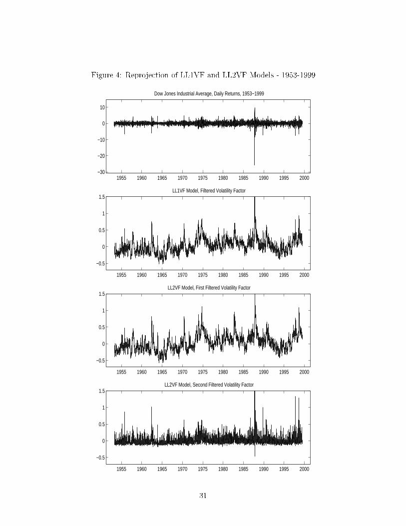
factors are latent we use the reprojection method of Gallant and Tauchen (1998). Figures 2

through 5 report time series plots of the Dow Jones series as well as the one- and two-factor

reprojected volatilities for aÆne and logarithmic di�usions. The �rst two plots pertain to

AFF1V and AFF2V covering sample 1953-1999 (Figure 2) and a single year, namely 1998

(Figure 3). Likewise, Figrues 4 and 5 cover LL1VF and LL2VF for the same samples, i.e.

1953-1999 and 1998. The one-factor models yield reprojected volatilities which look very

similar regardless of the model speci�cation. Hence, the reprojected volatilities for AFF1V

and LL1VF exhibit many common time series patterns. These plots con�rm the �nding

of Andersen et al. (2000) and Benzoni (1998) who compare the empirical �t of logarithmic

and aÆne volatility models. Both model speci�citions are empirically indistinguishable and

produce similar and persistent volatility.

These �nding do not extend to two-factor speci�cations, which explains why we are able

to discriminate between the aÆne and logarithmic speci�cations. Over the entire sample,

i.e. 1953-1999, we note that the �rst factor in AFF2V and LL2VF features the long run

persistent volatility uctuations. Given the long sample this may not be directly apparent

since the reprojected U3t factor still looks erratic. We plotted a single year from the sample,

namely 1998, to highlight that the �rst factor picks up persistence (see Figures 3 and 5),

and in fact resembles very much the single factor model reprojected volatilities (for the aÆne

model speci�cation more so than for the logarithmic one). The second factor for the AFF2V

and LL2VF speci�cations look very di�erent. This is apparent from both the entire sample

plots in Figures 2 and 4 as well as the 1998 reprojected volatilities. Particularly for the latter

18

we notice that with the aÆne speci�cation the second factor hardly moves (hence the �rst

factor resembles so closely the one-factor model reprojected volatility). For the logarithmic

volatility model we notice that the reprojected path of U4t features the local exhuberance

around the summer of 1998 when LTCM and the Russian �nancial crisis shook �nancial

markets.

4 Conclusion

In this paper we examine various two-factor SV models using the EMM estimation procedure

applied to a sample of post-war Dow Jones daily return series. The motivation to examine

two-factor models is the empirical failure of one-factor aÆne, Constant Elasticity of Variance

(CEV) and one-factor logarithmic SV models. We explored and compared the following two-

factor speci�cations (1) a continuous path aÆne di�usion factor process augmented with a

jump component to better �t the tail behavior, (2) a two-factor logarithmic SV speci�cation

with possible feedback, the latter causing volatility of volatility to increase, and (3) the

two factor aÆne SV model. We report that the speci�cation (2) is empirically the most

successful and provides a superior �t when compared, using a common SNP score, to the

two alternative two-factor speci�cations.

All two-factor speci�cations feature one factor which accounts for the the persistence in

volatility and the second determines the tail behavior. The empirical success of the loga-

rithmic speci�cation can intuitively be explained by the fact that the second factor not only

accommodates the tails of the (conditional) return distribution, but also accommodates the

volatility dynamics during extreme market conditions, since the speci�cation of the second

factor is mean-reverting with local persistence and state-dependent volatility of volatility.

Neither the jump process nor an aÆne di�usion as a second factor has such features.

It should also be noted that the two-factor logarithmic speci�cation avoids many complex

econometric as well as �nancial issues. We noted the problems in identifying the jump

intensity parameter. Andersen et al. (1999) resolved the identi�cation of jump intensity

via the smoothing of discrete jumps in simulations while we opted for a pro�ling procedure

(i.e. grid-seaching). The presence of jumps also considerably complicates the extraction

of the latent volatility and jump components since traditional �lters no longer apply. In

contrast, the continuous path two-factor logarithmic SV process does not pose any diÆculties

for �ltering via reprojection. We saw with the examples of one-factor speci�cations, that

di�erent types of models can generate similar returns dynamics. Therefore, the ultimate

19

contribution of the LL2VF model can be determined only after more stringent testing. For

instance, considering options data in addition to the underlying returns may be very useful.

They contain information regarding the tails of return distribution and, therefore, will allow

to separate competeing models of extreme events. This is subject of the future research.

There are other appealing properties to the two-factor logarithmic SV model. While

there are no analytic option-pricing solutions, the model has a smaller number of risk factors

compared to many of the alternative speci�cations. A good example is the aÆne jump

di�usion for which analytic option pricing formula are available. In such a model there is

a price of jump risk and a price of risk size, in addition to the �rst factor volatility risk

price and return risk common to all competing model speci�cations. Hence, there is at least

one additional price of risk to specify compared to the two-factor logarithmic speci�cation.

Moreover, complex speci�cations of the jump process with state-dependent jump intensity,

as discussed for instance in Chernov et al. (1999) and Pan (1999), result in an even larger

number of prices of risk.

Last, but not least, there are many �nancial complexities with the hedging of jump

processes. Again, the SV processes we �nd to be empirically superior belong to the type of

stochastic processes for which hedging strategies are straightforward extensions of standard

textbook material.

20

References

[1] Andersen, T., L. Benzoni and J. Lund (1999): Estimating Jump-Di�usions for Equity

Returns, Working Paper.

[2] Amin, K.I. and V.K Ng (1993): Option Valuation with Systematic Stochastic Volatility,

Journal of Finance 48, 881-910.

[3] Alizadeh, S., M.W. Brandt and F.X. Diebold (1999): Range-based Estimation of

Stochastic Volatility Models, Discussion Paper University of Pennsylvania.

[4] Baillie, R. T., T. Bollerslev, and H.-O. Mikkelsen, 1996, Fractionally integrated gener-

alized autoregressive conditional heteroskedasticity, Journal of Econometrics 74, 3-30.

[5] Ball, C. and W. Torous (1983): A Simpli�ed Jump Process for Common Stock Returns,

Journal of Financial and Quantitative Analysis, 18, 53-61.

[6] Ball, C. and W. Torous (1985): On Jumps in Common Stock Prices and Their Impact

on Call Option Pricing, Journal of Finance, 40, 155-173.

[7] Bakshi, G., C. Cao and Z. Chen (1997a): Empirical performance of alternative option

pricing models, Journal of Finance, 52, 2003-2049.

[8] Bakshi, G. and D. Madan (2000): Spanning and Derivative-Security Valuation, Journal

of Financial Economics, 55, 205-238.

[9] Bates, D. (1996a): Jumps and Stochastic Volatility: Exchange Rate Processes Implicit

in Deutsche Mark Options, Review of Financial Studies, 9, 69-107.

[10] Bates, D.S. (1996b): Testing Option Pricing Models. In Maddala, G.S. and C.R. Rao

(eds.), Handbook of Statistics, Vol. 14, Elsevier Science B.V.

[11] Bates, D. (2000): Post-'87 Crash Fears in the S&P 500 Futures Option Market, Journal

of Econometrics, 94, 181-238.

[12] Benzoni, L. (1998): Pricing Options Under Stochastic Volatility: An Econometric Anal-

ysis, Working Paper.

[13] Bollerslev, T., R. Engle and D. Nelson (1994): ARCH Models, in R. Engle and D.

McFadden (eds.) Handbook of Econometrics, Vol. 4, Elsevier Science B.V.

21

[14] Brace, A., D. Gatarek, and M. Musiela (1997): The Market Model of Interest Rate

Dynamics, Mathematical Finance, 7, 127-155

[15] Campbell, J., A. Lo and C. MacKinlay (1997): The Econometrics of Financial Markets,

Princeton University Press.

[16] Chernov, M. and E. Ghysels (2000): A study towards a uni�ed approach to the joint

estimation of objective and risk neutral measures for the purpose of options valuation,

Journal of Financial Economics 56, 407-458.

[17] Chernov, M., A.R. Gallant, E. Ghysels and G. Tauchen (1999): A New Class of Stochas-

tic Volatility Models with Jumps: Theory and Estimation, Discussion Paper.

[18] Chung, K. L. and R.J. Williams (1990): Introduction to Stochastic Integration, 2nd

edition, Birkh�auser.

[19] Conley, T., L. Hansen., and W.-F. Liu (1997): Bootstarpping the Long Run, Macroe-

conomic Dynamics, 1, 279-311

[20] Dai, Q. and K. Singleton (2000): Speci�cation Analysis of AÆne Term Structure Models,

Journal of Finance, (forthcoming).

[21] Das, S. and R. Sundaram (1997): Of Smiles and Smirks: A Term-Structure Perspective,

Working Paper, Harvard University

[22] Duan, J.C. (1995): The GARCH option pricing model, Mathematical Finance, 5, 13-32

[23] DuÆe, D. and R. Kan (1996): A Yield-Factor Model of Interest Rates, Mathematical

Finance, 6, 379-406

[24] DuÆe, D., J. Pan and K. Singleton (2000): Transform Analysis and Option Pricing for

AÆne Jump-Di�usions, Econometrica, 68, 1343-1377.

[25] Durham, G. and A.R. Gallant (2000): Numerical Techniques for Maximum Likeli-

hood Estimation of Continuous-Time Di�usion Processes, Working Paper, University

of North Carolina.

[26] Engle, R.F. and G. Lee (1999): A Long-Run and Short-Run Component Model of

Stock Return Volatility, in R.F. Engle and H. White (eds.) Cointegration, Causality

and Forecasting - A Festschrift in Honour of Clive W. J. Granger, Oxford University

Press.

22

[27] Eraker, B., M. Johannes and N. Polson (1999): Return Dynamics with Jumps to

Stochastic Volatility and Returns, Discussion Paper, Graduate School of Business, Uni-

versity of Chicago.

[28] Fenton, V.M. and A.R. Gallant (1996): Qualitative and Asymptotic Performance of

SNP Density Estimators, Journal of Econometrics 74, 77-118.

[29] Foster, D. and D. Nelson (1996): Continuous Record Asymptotics for Rolling Sample

Estimators, Econometrica, 64, 139-174.

[30] Gallant, A.R., D. Hsieh and G. Tauchen (1997): Estimation of stochastic volatility

models with diagnostics, Journal of Econometrics, 81, 159-192.

[31] Gallant, A.R., C.-T. Hsu and G.Tauchen (1999): Using Daily Range Data to Calibrate

Volatility Di�usions and Extract the Forward Integrated Variance, Review of Economics

and Statistics, (forthcoming).

[32] Gallant, A.R. and J. R. Long (1997): Estimating Stochastic Di�erential Equations

EÆciently by Minimum Chi-Square, Biometrika, 84, 125-141.

[33] Gallant, A.R., P.E. Rossi and G. Tauchen (1992): Stock Prices and Volume, Review of

Financial Studies, 5, 199-242.

[34] Gallant, A.R. and G. Tauchen (1989): Seminonparametric Estimation of Conditionally

Constrained Heterogeneous Processes: Asset Pricing Applications, Econometrica, 57,

1091-1120.

[35] Gallant, A.R. and G. Tauchen (1993): SNP: A Program for Nonparametric Time Series

Analysis, version 8.3, User's Guide, Discussion paper, University of North Carolina at

Chapel Hill.

[36] Gallant, A.R. and G. Tauchen (1996): Which Moments to Match? Econometric Theory,

12, 657-681.

[37] Gallant, A.R. and G. Tauchen (1997): EMM: a program for eÆcient method of moments

estimation, Version 1.4, User's guide, Discussion paper, University of North Carolina at

Chapel Hill.

[38] Gallant, A.R. and G. Tauchen (1998): Reprojecting Partially Observed Systems with

Application to Interest Rate Di�usions, Journal of American Statistical Association, 93,

10-24.

23

[39] Ghysels, E., A. Harvey and E. Renault (1996): Stochastic Volatility, in Maddala, G.S.

and C.R. Rao (eds.): Handbook of Statistics, Vol. 14, Elsevier Science B.V.

[40] Heston, S.L. (1993): A Closed-Form Solution for Options with Stochastic Volatility with

Applications to Bond and Currency Options, Review of Financial Studies, 6, 327-343.

[41] Heston, S.L. and S. Nandi (2000): A Closed-Form GARCH Option Pricing Model,

Review of Financial Studies, 13, 585-625.

[42] Ho, M., W. Perraudin and B. S�rensen (1996): A Continuous-Time Arbitrage-Pricing

Model With Stochastic Volatility and Jumps, Journal of Business and Economic Statis-

tics, 14, 31-43.

[43] Hull, J. and A. White (1987): The pricing of options on assets with stochastic volatilities,

Journal of Finance, 42, 281-300.

[44] Jacquier, E., N.G. Polson and P.E. Rossi (1994): Bayesian Analysis of Stochastic Volatil-

ity Models (with discussion): Journal of Business and Economic Statistics, 12, 371-417.

[45] Jarrow, R.A. and E. Rosenfeld (1984): Jump Risks and the Intertemporal Capital Asset

Pricing Model, Journal of Business, 57, 337-351.

[46] Johannes, M., R. Kumar and N.G. Polson (1999): State Dependent Jump Models: How

do US Equity Indices Jump?, Discussion Paper, Graduate School of Business, University

of Chicago.

[47] Jones, C. (1999): The Dynamics of Stochastic Volatility, Discussion Paper, University

of Rochester.

[48] Jorion, P. (1988): On Jump Processes in the Foreign Exchange and Stock Markets,

Review of Financial Studies, 1, 427-445.

[49] Kloeden, P.E. and E. Platen (1995): Numerical Solution of Stochastic Di�erential Equa-

tions, Springer Verlag.

[50] Krylov, N. V. (1995): Introduction to the Theory of Di�usion Processes, American

Mathematical Society.

[51] Lewis, A. (2000): Option Valuation Under Stochastic Volatility with Mathematica Code,

Finance Press.

24

[52] Nelson, D.: (1991) Conditional Heteroskedasticity in Asset Returns: a New Approach,

Econometrica 59, 347-370.

[53] Pan, J. (1999): Integrated Time-Series Analysis of Spot and Option Prices, Discussion

Paper, Graduate School of Business, Stanford University.

[54] Renault, E. (1997): Econometric models of option pricing errors. In Kreps, D.M. and

K.F. Wallis (eds.): Advances in economics and econometrics: Theory and applications,

Seventh World Congress, Vol. 3, Cambridge University Press.

[55] Schwert, G. W. (1990): Indexes of U.S. Stock Prices from 1802 to 1987, Journal of

Business, 63, 399-426.

[56] Scott, L. (1997): Pricing Stock Options in a Jump-Di�usion Model with Stochastic

Volatility and Interest Rates: Applications of Fourier Inversion Methods, Mathematical

Finance, 7, 413-426.

[57] Tauchen, G. (1997): New Minimum Chi-square methods in empirical �nance. In Kreps,

D.M. and K.F. Wallis (eds.): Advances in economics and econometrics: Theory and

applications, Seventh World Congress, Vol. 3, Cambridge University Press.

[58] Wiggins, J. B. (1987): Option values under stochastic volatility: Theory and empirical

estimates, Journal of Financial Economics, 19, 351-372.

25

A Regularity Conditions for Logarithmic Models

The use of logarithmic volatility models raises several issues regarding regularity condi-

tions which ensure existence of moments, strong solutions to stochastic di�erence equations

(SDEs), well-de�ned option prices and convergence of discretization schemes. For the class of

aÆne models such conditions are well established, see for instance DuÆe, Pan and Singleton

(2000) and Kloeden and Platen (1995) for elaborate discussion of the various issues.

For logarithmic SV models these issues are not so well-documented and more involved.

In particular, the stochastic integrals associated with the SDEs of the logarithmic SV class

are not de�ned in the usual sense (the integrand has to be in L2; e.g. Krylov, 1995, p.

91).8 The exponential transformation of the volatility factors results in explosive behavior.

The explosiveness of the logarithmic SV process has been recognized for a while in the term

structure literature. For instance, Brace et al. (1997) replace the continously compounded

rate by the e�ective annual rate. This removes the exponentiation of a lognormal variable,

which in its turn removes fatness in the tail, so that the moments exist.

There several issues which help us circumvent the ill-behaved asymptotic features. The

scope of �nancial applications, which typically involves a �nite horizon, allows us to consider

a weaker de�nition of the stochastic integral for the localized integrand (Krylov, 1995, p. 95

and Lewis (2000)). We inforce this de�nition via our simulation scheme, where we efectively

localize the process.

We also have to ensure that solutions to the speci�ed logarithmic SV processes exist and

are unique. The processes we consider do satisfy the local Lipshitz conditions, but violate the

usual growth conditions in Ito's theorem (Krylov, 1995, Remark on p. 167). The logarithmic

SV processes satisfy the weaker growth condition (Krylov, 1995, Theorem on p. 166). This

weaker growth condition is satis�ed because the drift of the log-return process U1 contains

the Ito formula correction term, which is equal to a negative half of the variance. Hence, the

potentially explosive variance cancels out. Krylov (1995) also shows the convergence of the

Euler SDE discretization scheme for such processes (Section V.3).

The potential explosiveness of the variance process puts the stationarity of logarithmic

SV processes into doubt. This issue is especially important since asymptotic results of EMM

rely on the stationarity assumptions. The key implication of stationarity is that moments do

not grow with horizon, a feature which was veri�ed via simulation by computing moments

of di�erent sample sizes.

Finally, in �nance, we are quite often interested in the moments of the price level, i.e.

8We are greatful to Nour Meddahi for pointing this out to us.

26

expU1: Let us describe the problem in stylized notations. If expU1 has independent drift �t

and variance Vt; then we can write the �rst moment as follows:

E�eU1t

�= E

�eR t0(�s� 1

2Vs)ds+

R t0

pVsdWs

�= E

�eR t0�sds

�� E

�e�

1

2

R t0Vsds+

R t0

pVsdWs

�(23)

Chung and Williams (1990 Theorem 6.2) show that ifR t0

pVsdWs is a local martingale, then

the second term under the expectation operator is a local martingale.9 Therefore, given our

understanding of the weaker de�nition of the stochastic integral, we know that for logarithmic

SV processes that term is a local martingale.

9Note that ifR t0

pVsdWs is a martingale and the Novikov condition is satis�ed, then this term is a

martingale.

27

1950 1955 1960 1965 1970 1975 1980 1985 1990 1995 2000

−25

−20

−15

−10

−5

0

5

10

15

20

25

Dow Jones Industrials, 1953−1999

Figures and Tables

Figure 1: Dow Jones Industrial Average 1953 - 1999

28

1955 1960 1965 1970 1975 1980 1985 1990 1995 2000−30

−20

−10

0

10

Dow Jones Industrial Average, Daily Returns, 1953−1999

1955 1960 1965 1970 1975 1980 1985 1990 1995 2000

−6

−4

−2

0

2

4

AFF1V Model, Filtered Log Volatility Factor

1955 1960 1965 1970 1975 1980 1985 1990 1995 2000

−6

−4

−2

0

2

4

AFF2V Model, First Filtered Log Volatility Factor

1955 1960 1965 1970 1975 1980 1985 1990 1995 2000

−6

−4

−2

0

2

4

AFF2V Model, Second Filtered Log Volatility Factor

Figure 2: Reprojection of AFF1V and AFF2V Models - 1953-1999

29

1998 1998.1 1998.2 1998.3 1998.4 1998.5 1998.6 1998.7 1998.8 1998.9 1999

−10

−5

0

5

Dow Jones Industrial Average, Daily Returns, 1998

1998 1998.1 1998.2 1998.3 1998.4 1998.5 1998.6 1998.7 1998.8 1998.9 1999

−6

−4

−2

0

2

4

aff1v Model, Filtered Log Volatility Factor

1998 1998.1 1998.2 1998.3 1998.4 1998.5 1998.6 1998.7 1998.8 1998.9 1999

−6

−4

−2

0

2

4

aff2v Model, First Log Filtered Volatility Factor

1998 1998.1 1998.2 1998.3 1998.4 1998.5 1998.6 1998.7 1998.8 1998.9 1999

−6

−4

−2

0

2

4

aff2v Model, Second Log Filtered Volatility Factor

Figure 3: Reprojection of AFF1V and AFF2V Models - 1998

30

1955 1960 1965 1970 1975 1980 1985 1990 1995 2000−30

−20

−10

0

10

Dow Jones Industrial Average, Daily Returns, 1953−1999

1955 1960 1965 1970 1975 1980 1985 1990 1995 2000

−0.5

0

0.5

1

1.5LL1VF Model, Filtered Volatility Factor

1955 1960 1965 1970 1975 1980 1985 1990 1995 2000

−0.5

0

0.5

1

1.5LL2VF Model, First Filtered Volatility Factor

1955 1960 1965 1970 1975 1980 1985 1990 1995 2000

−0.5

0

0.5

1

1.5LL2VF Model, Second Filtered Volatility Factor

Figure 4: Reprojection of LL1VF and LL2VF Models - 1953-1999

31

1998 1998.1 1998.2 1998.3 1998.4 1998.5 1998.6 1998.7 1998.8 1998.9 1999

−10

−5

0

5

Dow Jones Industrial Average, Daily Returns, 1998

1998 1998.1 1998.2 1998.3 1998.4 1998.5 1998.6 1998.7 1998.8 1998.9 1999

−0.5

0

0.5

1

1.5LL1VF Model, Filtered Volatility Factor

1998 1998.1 1998.2 1998.3 1998.4 1998.5 1998.6 1998.7 1998.8 1998.9 1999

−0.5

0

0.5

1

1.5LL2VF Model, First Filtered Volatility Factor

1998 1998.1 1998.2 1998.3 1998.4 1998.5 1998.6 1998.7 1998.8 1998.9 1999

−0.5

0

0.5

1

1.5LL2VF Model, Second Filtered Volatility Factor

Figure 5: Reprojection of LL1VF and LL2VF Models - 1998

32

Table 1. Model De�nitions and Minimized Chi-Squared Criterion.

�10 �12 �22 �30 �33 �40 �44 �10 �13 �14 �33 �44 13 14 �J �J N �2(�) df p-value

AFF1V * * * * * * 1 * 50k 29.787 9 0.0001

AFF1V * * * * * * 1 * 75k 29.098 9 0.0002

AFF1V * * * * * * 1 * 100k 30.687 9 0.0001

LL1V * * * * * * * 50k 38.613 9 0.1e-04

LL1V * * * * * * * 75k 31.375 9 0.4e-04

LL1V * * * * * * * 100k 30.866 9 0.1e-04

LL1VF * * * * * * * * 50k 27.074 8 .0007

LL1VF * * * * * * * * 75k 28.117 8 .0005

LL1VF * * * * * * * * 100k 25.290 8 .001

AFF2V * * * * * * * * * 1 1 * * 50k 22.224 5 0.0002

AFF2V * * * * * * * * * 1 1 * * 75k 23.139 5 0.0001

AFF2V * * * * * * * * * 1 1 * * 100k 25.300 5 0.5e-04

AFF1V-J * * * * * * 1 * 5.60 * 50k 28.276 8 0.0002

AFF1V-J * * * * * * 1 * 5.60 * 75k 18.355 8 0.0067

AFF1V-J * * * * * * 1 * 5.60 * 100k 20.806 8 0.0028

LL2V * * * * * * * * * * * * 50k 21.377 6 .002

LL2V * * * * * * * * * * * * 75k 20.334 6 .002

LL2V * * * * * * * * * * * * 100k 17.075 6 .002

LL2VF * * * * * * * * * * * * 50k 8.205 4 .084

LL2VF * * * * * * * * * * * * 75k 7.419 4 .115

LL2VF * * * * * * * * * * * * 100k 9.539 4 .049

Notes: * denotes a free parameter; 1 denotes a parameter pinned at unity; blank denotes

a parameter set to zero. 100k denotes a simulation of length N = 100; 000 simulated at

1=� = 6048 steps per year, or, equivalently 24 steps per day with 252 trading days per year.

33

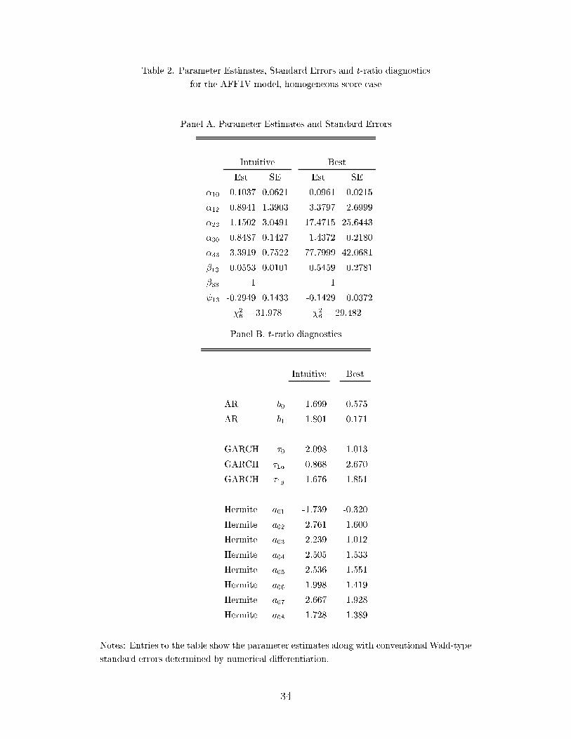
Table 2. Parameter Estimates, Standard Errors and t-ratio diagnostics

for the AFF1V model, homogeneous score case

Panel A. Parameter Estimates and Standard Errors

Intuitive Best

Est SE Est SE

�10 0.1037 0.0621 0.0961 0.0215

�12 0.8941 1.3903 3.3797 2.6999

�22 -1.1502 3.0491 -17.4715 25.6443

�30 0.8487 0.1427 1.4372 0.2180

�33 -3.3919 0.7522 -77.7999 42.0681

�13 0.0553 0.0101 0.5459 0.2781

�33 1 1

13 -0.2949 0.1433 -0.1429 0.0372

�26= 31:978 �2

6= 29:482

Panel B. t-ratio diagnostics

Intuitive Best

AR b0 -1.699 0.575

AR b1 1.801 0.171

GARCH �0 2.098 1.013

GARCH �1a 0.868 2.670

GARCH �1g 1.676 1.851

Hermite a01 -1.739 -0.320

Hermite a02 2.761 1.600

Hermite a03 -2.239 -1.012

Hermite a04 2.505 1.533

Hermite a05 -2.536 -1.551

Hermite a06 1.998 1.419

Hermite a07 -2.667 -1.928

Hermite a08 1.728 1.389

Notes: Entries to the table show the parameter estimates along with conventional Wald-type

standard errors determined by numerical di�erentiation.

34

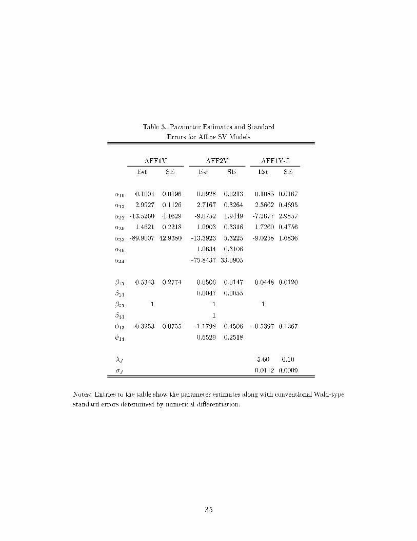
Table 3. Parameter Estimates and Standard

Errors for AÆne SV Models

AFF1V AFF2V AFF1V-J

Est SE Est SE Est SE

�10 0.1004 0.0196 0.0928 0.0213 0.1085 0.0167

�12 2.9927 0.1126 2.7167 0.3264 2.3662 0.4695

�22 -13.5260 4.1629 -9.0752 1.9449 -7.2677 2.9857

�30 1.4621 0.2218 1.0903 0.3316 1.7260 0.4756

�33 -89.9007 42.9380 -13.3923 5.3225 -9.0258 1.6836

�40 1.0634 0.3106

�44 -75.8437 33.0905

�13 0.5343 0.2774 0.0506 0.0147 0.0448 0.0120

�14 0.0047 0.0055

�33 1 1 1

�44 1

13 -0.3253 0.0755 -1.1798 0.4506 -0.5397 0.1367

14 0.6529 0.2518

�J 5.60 0.10

�J 0.0112 0.0009

Notes: Entries to the table show the parameter estimates along with conventional Wald-type

standard errors determined by numerical di�erentiation.

35

Table 4. Parameter Estimates and Standard

Errors for Logarithmic SV Models

Est SE Est SE

One Volatility Factor

LL1V LL1VF

�10 0.0780 0.0199 0.0624 0.0207

�12 0.8584 0.0348 1.2240 0.1629

�22 -0.9766 0.0911 -1.8576 0.4109

�33 -4.5825 0.5282 -2.8438 0.2720

�10 -2.6131 0.0346 -2.9725 0.0259

�13 1.1549 0.0370 1.0096 0.0233

�33 0.6999 0.0990

13 -0.9930 0.0253 -1.8534 0.0451

Two Volatility Factors

LL2V LL2VF

�10 0.0775 0.0218 0.0585 0.0245

�12 1.0266 0.4181 1.0238 0.6858

�22 -1.3253 1.1033 -1.3151 1.6807

�33 -0.0079 0.0021 -0.0684 0.1679

�44 -70.2041 19.2029 -52.5609 10.0369

�10 -2.3614 0.0797 -2.3918 0.0797

�13 0.0419 0.0324 0.0946 0.1774

�14 3.4352 0.4725 2.7558 0.4115

�33 0.2404 1.0879

�44 1.2047 1.8136

13 -0.5592 0.1859 -0.3034 0.0887

14 -0.4138 0.0929 -0.4179 0.1049

Notes: Entries to the table show the parameter estimates along with conventional Wald-type

standard errors determined by numerical di�erentiation. It is shown in section 3 that the

apparent insigni�cance of the estimates of �33 and �44; is a result of the failure of the Wald-

based statistics to capture asymmetric con�dence sets. Approximate con�dence intervals

can be constructed by inverting the chi-squared criterion function (see Gallant and Tauchen

(1997, 2000)) and are reported in section 3.

36

Table 5. t-Ratio Diagnostics

LLV1 LLV1F LLV2 LLV2F AFFV1 AFFV2 AFFV1-J

AR b0 -0.618 -0.539 0.117 0.126 0.506 -0.422 -0.385

AR b1 0.452 0.073 0.123 0.122 0.317 -0.157 0.596

GARCH �0 1.913 1.422 1.590 1.331 1.984 1.626 1.550

GARCH �1a 1.543 0.780 1.897 1.408 3.400 1.816 1.716

GARCH �1g 1.722 1.114 1.823 1.407 2.826 1.590 1.757

Hermite a10 -0.204 -0.062 -0.877 -0.196 -0.133 0.547 -0.760

Hermite a01 0.206 -0.036 0.788 0.742 0.724 0.561 -0.917

Hermite a11 0.859 -0.296 0.388 0.075 0.465 0.343 0.657

Hermite a02 2.820 1.875 0.997 1.033 2.125 1.559 2.062

Hermite a12 -1.066 -0.937 -1.735 -0.747 -1.347 -0.887 -1.489

Hermite a03 -0.619 -0.848 0.856 0.741 0.509 -0.113 -1.019

Hermite a04 3.257 1.916 0.883 0.806 1.857 1.979 2.207

Hermite a05 -1.648 -1.657 0.044 0.143 -0.278 -1.346 -1.104

Hermite a06 2.858 1.435 0.873 0.486 1.781 2.104 1.881

Hermite a07 -2.126 -2.012 -0.618 -0.317 -0.814 -1.979 -1.200

Hermite a08 2.492 1.315 1.009 0.445 1.806 2.175 1.664

37