absolute momentum: a simple rule-based strategy and ... · pdf file1 absolute momentum: a...

1

Absolute Momentum: a Simple Rule-Based Strategy and Universal

Trend-Following Overlay

Gary Antonacci

Portfolio Management Associates, LLC1

February 28, 2013

Abstract

There is a considerable body of research on relative strength price momentum but

relatively little on absolute, time series momentum. In this paper, we explore the

practical side of absolute momentum. We first explore its sole parameter - the

formation, or look back, period. We then examine the reward, risk, and correlation

characteristics of absolute momentum applied to stocks, bonds, and real assets. We

finally apply absolute momentum to a 60-40 stock/bond portfolio and a simple risk

parity portfolio. We show that absolute momentum can effectively identify regime

change and add significant value as an easy to implement, rule-based approach with

many potential uses as both a stand- alone program and trend following overlay.

1 http://optimalmomentum.com

2

1. Introduction

The cross-sectional momentum effect is one of the strongest and most pervasive

financial phenomena (Jegadeesh and Titman (1993), (2001)). Researchers have verified

its value with many different asset classes, as well as across groups of assets (Blitz and

Van Vliet (2008), Asness, Moskowitz and Pedersen (2012)). Since its publication,

momentum has held up out-of-sample going forward in time (Grundy and Martin

(2001), Asness, Moskowitz and Pedersen (2012)) and back to the Victorian Age

(Chabot, Ghysels, and Jagannathan (2009)).

In addition to cross-sectional momentum, in which an asset's performance

relative to other assets predicts its future relative performance, momentum also works

well on an absolute, or time series basis, in which an asset's own past return predicts its

future performance. In absolute momentum there is significant positive auto-covariance

between an asset's excess return next month and its lagged one-year return (Moskowitz,

Ooi and Pedersen (2012)).

Absolute momentum is therefore trend following by nature. Trend following

methods, in general, have slowly achieved recognition and acceptance in the academic

community (Brock, Lakonishok and LeBaron (1992), Lo, Mamaysky, and Wang

(2000), Zhu and Zhou (2009), Han, Yang, and Zhou (2011)).

Absolute momentum appears to be just as robust and universally applicable as

cross-sectional momentum. It performs well in extreme market environments, across

3

multiple asset classes (commodities, equity indices, bond markets, currency pairs), and

back in time to the turn of the century (Hurst, Ooi, and Pedersen (2012)).

Despite an abundance of momentum research over the past twenty years, no one

is sure why it works so well. The most common explanations for both momentum and

trend following profits have to do with behavioral factors, such as anchoring, herding,

and the disposition effect (Tversky and Kahneman (1974), Barberis, Shleifer, and

Vishny (1998), Daniel, Hirshleifer, and Subrahmanyam (1998), Hong and Stein (1999),

Frazzini (2006)).

In anchoring, investors are slow to react to new information, which leads initially

to under reaction. In herding, buying begets more buying and causes prices to over react

and move beyond fundamental value after the initial under reaction. Through the

disposition effect, investors sell winners too soon and hold losers too long. This creates

a headwind making trends continue longer before reaching true value.

Risk management schemes that sell in down markets and buy in up markets can

also cause trends to persist (Garleanu and Pedersen (2007)), as can confirmation bias,

which causes investors to look at recent price moves as representative of the future.

This then leads them to move money into investments that have recently appreciated,

thus causing trends to continue further (Tversky and Kahneman (1974)). Behavioral

biases are deeply rooted, which may explain why momentum profits have persisted and

are likely to continue to persist.

4

In this paper, we focus on absolute momentum because of its simplicity and the

advantages it holds for long-only investing. We can apply absolute momentum to any

asset or portfolio of assets without losing any of the contributory value of other assets.

With relative strength momentum, on the other hand, we have to exclude weaker assets

from the active portfolio. This can reduce the benefits that come from multi-asset

diversification and create opportunity loss by excluding assets that may suddenly start

outperforming.

The second advantage of absolute momentum is its superior ability to reduce

downside volatility and drawdown by identifying regime change. Both relative and

absolute momentum can enhance return, but absolute momentum, by its trend-following

nature, is much more effective in reducing the downside exposure associated with long-

only investing (Antonacci (2013)).

The next section of this paper describes our data and the methodology we use to

work with absolute momentum. The following section explores the formation period

used for determining absolute momentum. After that, we show what effect absolute

momentum has on the reward, risk, and correlation characteristics of a number of

diverse markets, compared to a buy and hold approach. Finally, we apply absolute

momentum to two representative multi-asset portfolios - a 60-40 balanced stock/bond

portfolio and a simple, diversified risk parity portfolio.

5

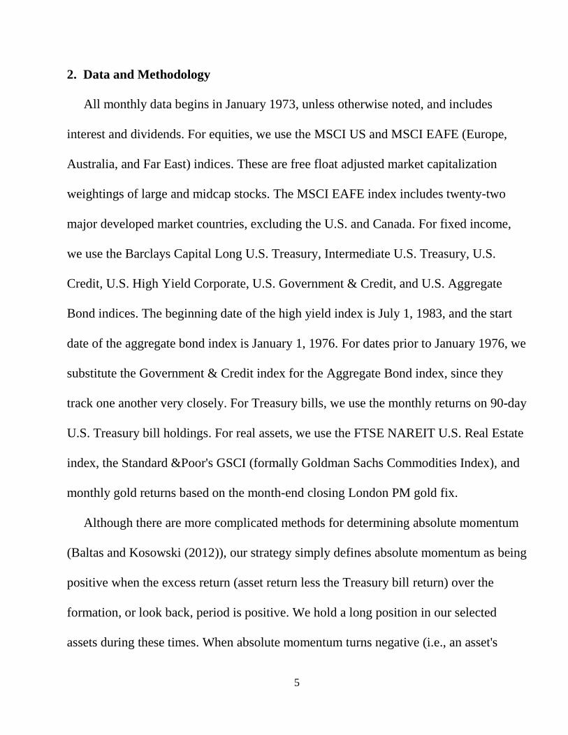
2. Data and Methodology

All monthly data begins in January 1973, unless otherwise noted, and includes

interest and dividends. For equities, we use the MSCI US and MSCI EAFE (Europe,

Australia, and Far East) indices. These are free float adjusted market capitalization

weightings of large and midcap stocks. The MSCI EAFE index includes twenty-two

major developed market countries, excluding the U.S. and Canada. For fixed income,

we use the Barclays Capital Long U.S. Treasury, Intermediate U.S. Treasury, U.S.

Credit, U.S. High Yield Corporate, U.S. Government & Credit, and U.S. Aggregate

Bond indices. The beginning date of the high yield index is July 1, 1983, and the start

date of the aggregate bond index is January 1, 1976. For dates prior to January 1976, we

substitute the Government & Credit index for the Aggregate Bond index, since they

track one another very closely. For Treasury bills, we use the monthly returns on 90-day

U.S. Treasury bill holdings. For real assets, we use the FTSE NAREIT U.S. Real Estate

index, the Standard &Poor's GSCI (formally Goldman Sachs Commodities Index), and

monthly gold returns based on the month-end closing London PM gold fix.

Although there are more complicated methods for determining absolute momentum

(Baltas and Kosowski (2012)), our strategy simply defines absolute momentum as being

positive when the excess return (asset return less the Treasury bill return) over the

formation, or look back, period is positive. We hold a long position in our selected

assets during these times. When absolute momentum turns negative (i.e., an asset's

6

excess return turns negative), our baseline strategy is to exit the asset and switch into

90-day U.S. Treasury bills until absolute momentum again becomes positive. Treasury

bills are a safe harbor for us during times of market stress.

We reevaluate and adjust positions on a monthly basis. The number of transactions

per year into or out of Treasury bills ranges from a low of 0.33 for REITs to a high of

1.08 for high yield bonds. We deduct 20 basis points per trade for transaction costs.

Maximum drawdown is the greatest peak-to-valley equity erosion on a month-end

basis.

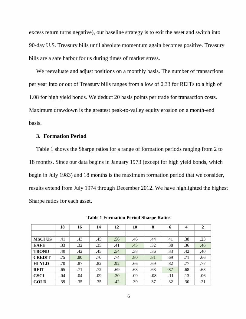
3. Formation Period

Table 1 shows the Sharpe ratios for a range of formation periods ranging from 2 to

18 months. Since our data begins in January 1973 (except for high yield bonds, which

begin in July 1983) and 18 months is the maximum formation period that we consider,

results extend from July 1974 through December 2012. We have highlighted the highest

Sharpe ratios for each asset.

Table 1 Formation Period Sharpe Ratios

18 16 14 12 10 8 6 4 2

MSCI US .41 .43 .45 .56 .46 .44 .41 .38 .23

EAFE .33 .32 .35 .41 .45 .32 .38 .36 .46

TBOND .40 .42 .45 .54 .38 .36 .33 .42 .40

CREDIT .75 .80 .70 .74 .80 .81 .69 .71 .66

HI YLD .70 .87 .82 .92 .66 .69 .82 .77 .77

REIT .65 .71 .72 .69 .63 .63 .87 .68 .63

GSCI .04 .04 .09 .20 .09 -.08 -.11 .13 .06

GOLD .39 .35 .35 .42 .39 .37 .32 .30 .21

7

Best results cluster at 12 months.2 As a check on this, we segment our data into

subsamples and find the highest Sharpe ratios for each asset in every decade from 1974

through 2012. Figure 1 shows the number of times the Sharpe ratio is highest (or within

two percentage points of being the highest) for each look back period across all the

decades.

Figure 1 Top Formation Periods 1974-2012

Our results coincide with the best formation periods of cross-sectional momentum,

which extend from 3 to 12 months and also cluster at 12 months3 (Jegadeesh and

Titman (1993)). Many momentum papers use a 12-month formation period with a 1-

2 We looked at monthly moving average penetrations as an alternative trend following filter and found no discernible

pattern of optimal values. 3 Cowles and Jones (1937) were the first to point out the profitable look back period of 12 months using U.S. stock market

data from 1920 through 1935.

0

1

2

3

4

5

6

7

8

9

18 16 14 12 10 8 6 4 2

O

c

c

u

r

a

n

c

e

s

Best Look Back Months

8

month holding period as a benchmark strategy for research purposes. Given its

dominance here and throughout the literature, we will also use a 12-month formation

period as our benchmark strategy. This should minimize the risk of data snooping.

4. Absolute Momentum Characteristics

Table 2 is a performance summary of each asset and the median of all the assets,

with and without 12-month absolute momentum.

Table 2 Absolute Momentum Results 1974-2012

Annual

Return

Annual

Std Dev

Annual

Sharpe

Maximum

Drawdown

% Profit

Months

MSCI US Abs Mom

12.26 11.57 .55 -22.90 75

MSCI US No Mom 11.62 15.74 .37 -50.65 61

EAFE Abs Mom 10.39 11.82 .39 -25.14 78

EAFE No Mom 11.56 17.53 .33 -56.40 60

TBOND Abs Mom 10.08 8.43 .52 -12.92 77

TBOND No Mom 9.74 10.54 .39 -20.08 61

CREDIT Abs Mom 8.91 4.72 .70 -8.70 82

CREDIT No Mom 8.77 7.18 .44 -19.26 67

HI YLD Abs Mom 9.97 4.76 .90 -7.14 88

HI YLD No Mom 10.05 8.70 .50 -33.31 75

REIT Abs Mom 14.16 11.74 .69 -19.97 75

REIT No Mom 14.74 17.25 .50 -68.30 62

GSCI Abs Mom 8.24 15.46 .17 -48.93 81

GSCI No Mom 4.93 19.96 -.02 -61.03 54

GOLD Abs Mom 13.68 16.62 .46 -24.78 81

GOLD No Mom 9.44 19.97 .19 -61.78 53

MEDIAN Abs Mom 10.25 11.66 .53 -21.43 79

MEDIAN No Mom 9.90 16.48 .38 -53.53 61

9

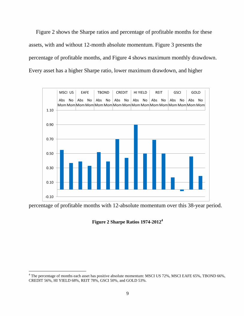
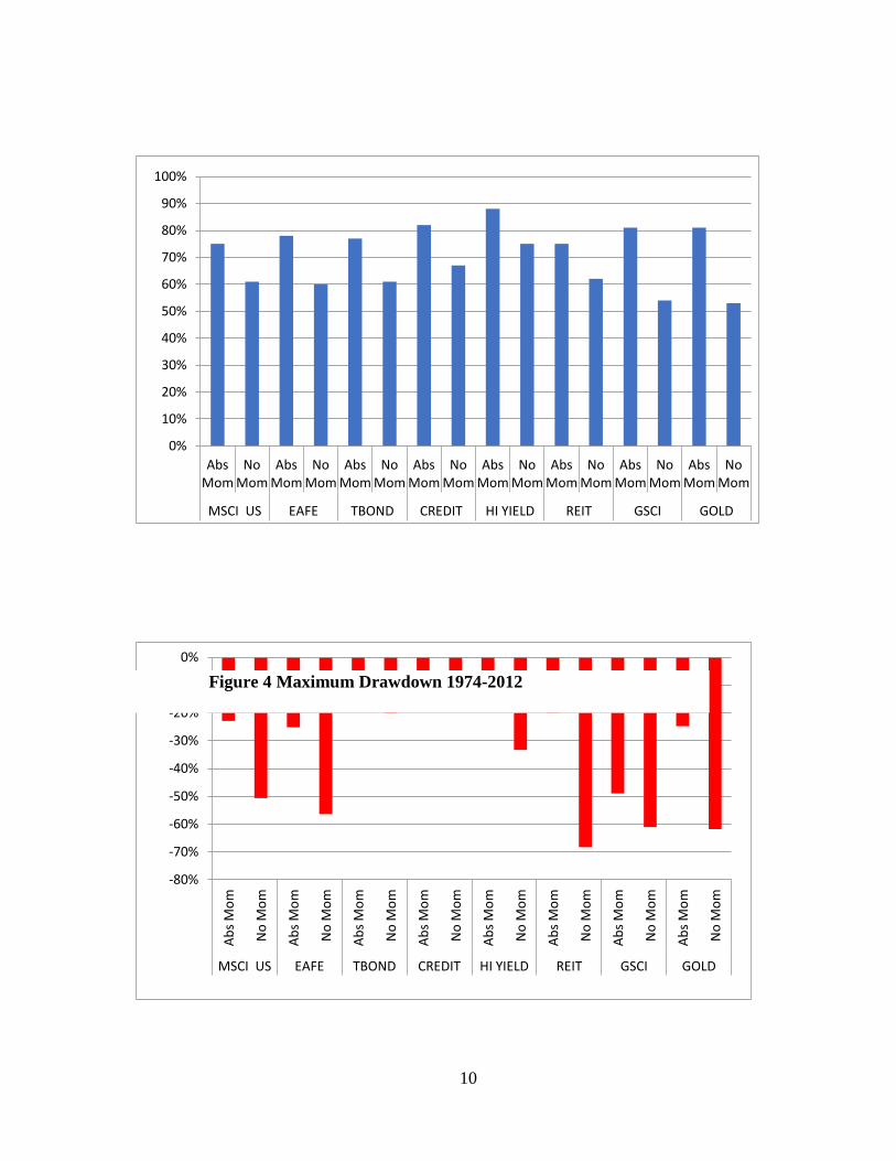
Figure 2 shows the Sharpe ratios and percentage of profitable months for these

assets, with and without 12-month absolute momentum. Figure 3 presents the

percentage of profitable months, and Figure 4 shows maximum monthly drawdown.

Every asset has a higher Sharpe ratio, lower maximum drawdown, and higher

percentage of profitable months with 12-absolute momentum over this 38-year period.

Figure 2 Sharpe Ratios 1974-20124

4 The percentage of months each asset has positive absolute momentum: MSCI US 72%, MSCI EAFE 65%, TBOND 66%,

CREDIT 56%, HI YIELD 68%, REIT 78%, GSCI 50%, and GOLD 53%.

-0.10

0.10

0.30

0.50

0.70

0.90

1.10

Abs Mom

No Mom

Abs Mom

No Mom

Abs Mom

No Mom

Abs Mom

No Mom

Abs Mom

No Mom

Abs Mom

No Mom

Abs Mom

No Mom

Abs Mom

No Mom

MSCI US EAFE TBOND CREDIT HI YIELD REIT GSCI GOLD

10

Figure 3 Percentage Profitable Months 1974-2012

0%

10%

20%

30%

40%

50%

60%

70%

80%

90%

100%

Abs Mom

No Mom

Abs Mom

No Mom

Abs Mom

No Mom

Abs Mom

No Mom

Abs Mom

No Mom

Abs Mom

No Mom

Abs Mom

No Mom

Abs Mom

No Mom


-80%

-70%

-60%

-50%

-40%

-30%

-20%

-10%

0%

Ab

s M

om

No

Mo

m

Ab

s M

om

No

Mo

m

Ab

s M

om

No

Mo

m

Ab

s M

om

No

Mo

m

Ab

s M

om

No

Mo

m

Ab

s M

om

No

Mo

m

Ab

s M

om

No

Mo

m

Ab

s M

om

No

Mo

m


Figure 4 Maximum Drawdown 1974-2012

11

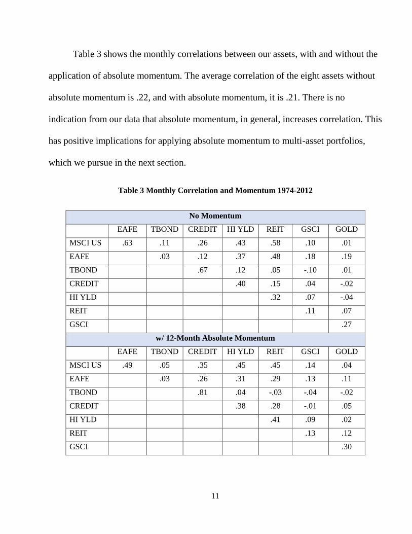
Table 3 shows the monthly correlations between our assets, with and without the

application of absolute momentum. The average correlation of the eight assets without

absolute momentum is .22, and with absolute momentum, it is .21. There is no

indication from our data that absolute momentum, in general, increases correlation. This

has positive implications for applying absolute momentum to multi-asset portfolios,

which we pursue in the next section.

Table 3 Monthly Correlation and Momentum 1974-2012

No Momentum

EAFE TBOND CREDIT HI YLD REIT GSCI GOLD

MSCI US .63 .11 .26 .43 .58 .10 .01

EAFE .03 .12 .37 .48 .18 .19

TBOND .67 .12 .05 -.10 .01

CREDIT .40 .15 .04 -.02

HI YLD .32 .07 -.04

REIT .11 .07

GSCI .27

w/ 12-Month Absolute Momentum

EAFE TBOND CREDIT HI YLD REIT GSCI GOLD

MSCI US .49 .05 .35 .45 .45 .14 .04

EAFE .03 .26 .31 .29 .13 .11

TBOND .81 .04 -.03 -.04 -.02

CREDIT .38 .28 -.01 .05

HI YLD .41 .09 .02

REIT .13 .12

GSCI .30

12

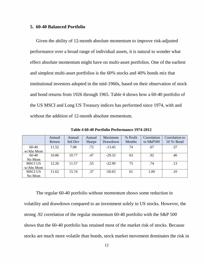
5. 60-40 Balanced Portfolio

Given the ability of 12-month absolute momentum to improve risk-adjusted

performance over a broad range of individual assets, it is natural to wonder what

effect absolute momentum might have on multi-asset portfolios. One of the earliest

and simplest multi-asset portfolios is the 60% stocks and 40% bonds mix that

institutional investors adopted in the mid-1960s, based on their observation of stock

and bond returns from 1926 through 1965. Table 4 shows how a 60-40 portfolio of

the US MSCI and Long US Treasury indices has performed since 1974, with and

without the addition of 12-month absolute momentum.

Table 4 60-40 Portfolio Performance 1974-2012

Annual

Return

Annual

Std Dev

Annual

Sharpe

Maximum

Drawdown

% Profit

Months

Correlation

to S&P500

Correlation to

10 Yr Bond

60-40

w/Abs Mom

11.52 7.88 .72 -13.45 74 .67 .37

60-40

No Mom

10.86 10.77 .47 -29.32 63 .92 .46

MSCI US

w/Abs Mom

12.26 11.57 .55 -22.90 75 .74 .13

MSCI US

No Mom

11.62 15.74 .37 -50.65 61 1.00 .10

The regular 60-40 portfolio without momentum shows some reduction in

volatility and drawdown compared to an investment solely in US stocks. However, the

strong .92 correlation of the regular momentum 60-40 portfolio with the S&P 500

shows that the 60-40 portfolio has retained most of the market risk of stocks. Because

stocks are much more volatile than bonds, stock market movement dominates the risk in

13

a 60-40 portfolio. From a risk perspective, the regular 60/40 portfolio is, in fact, mainly

an equity portfolio, since stock market variation explains nearly all the variation in

performance of the regular 60-40 portfolio.

The MSCI US index with the addition of absolute momentum has a .74

correlation to the S&P 500 index, which is lower than the correlation of the regular 60-

40 index. It does a better job than the 60-40 portfolio in reducing portfolio drawdown,

while also providing higher returns. The correlation to the S&P 500 of the 60-40

portfolio using 12-month absolute momentum drops to .67, indicating more reduction in

stock market exposure.5 The 60-40 portfolio with absolute momentum retains the same

return as the normal MSCU US index, but with only half the volatility. The maximum

drawdown drops by more than 70%.

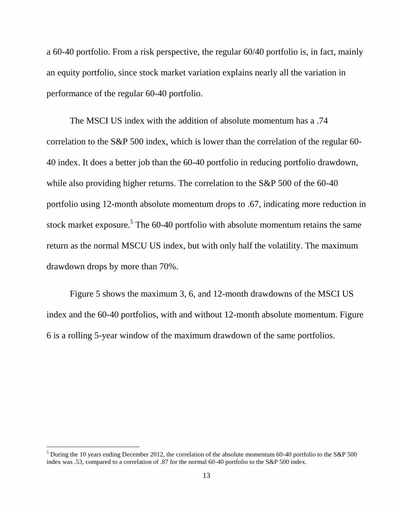
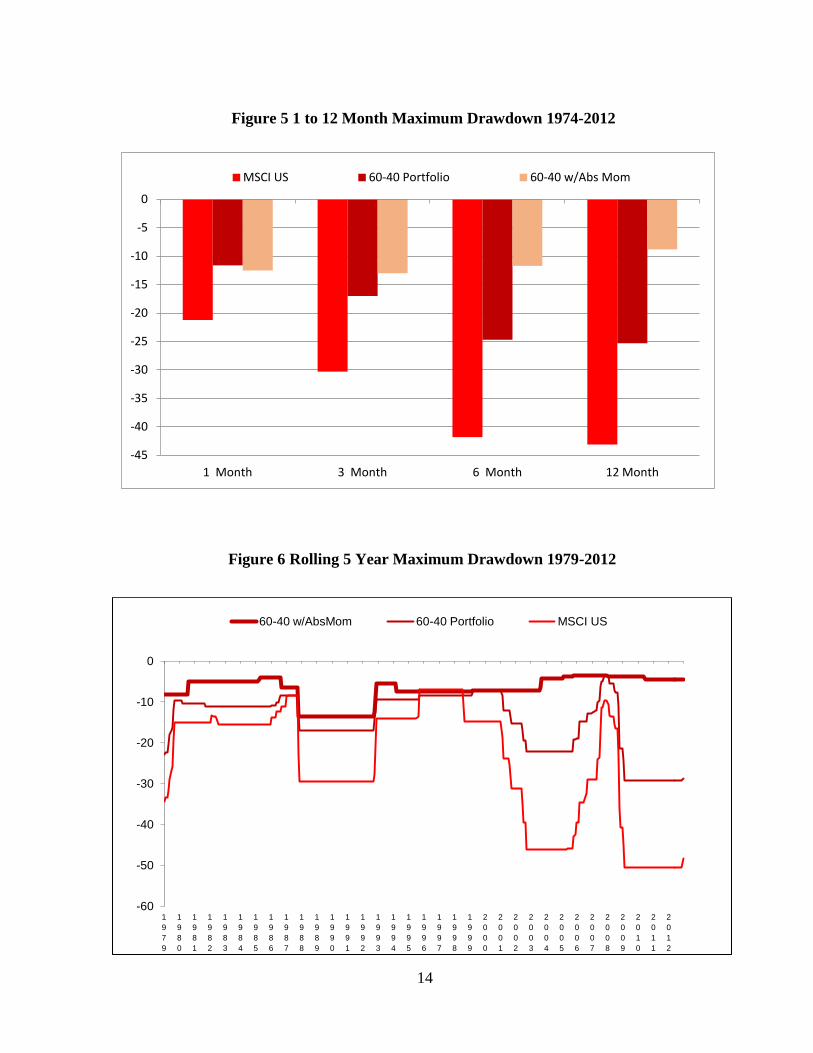
Figure 5 shows the maximum 3, 6, and 12-month drawdowns of the MSCI US

index and the 60-40 portfolios, with and without 12-month absolute momentum. Figure

6 is a rolling 5-year window of the maximum drawdown of the same portfolios.

5 During the 10 years ending December 2012, the correlation of the absolute momentum 60-40 portfolio to the S&P 500

index was .53, compared to a correlation of .87 for the normal 60-40 portfolio to the S&P 500 index.

14

Figure 5 1 to 12 Month Maximum Drawdown 1974-2012

-60

-50

-40

-30

-20

-10

0

1

9

7

9

1

9

8

0

1

9

8

1

1

9

8

2

1

9

8

3

1

9

8

4

1

9

8

5

1

9

8

6

1

9

8

7

1

9

8

8

1

9

8

9

1

9

9

0

1

9

9

1

1

9

9

2

1

9

9

3

1

9

9

4

1

9

9

5

1

9

9

6

1

9

9

7

1

9

9

8

1

9

9

9

2

0

0

0

2

0

0

1

2

0

0

2

2

0

0

3

2

0

0

4

2

0

0

5

2

0

0

6

2

0

0

7

2

0

0

8

2

0

0

9

2

0

1

0

2

0

1

1

2

0

1

2

60-40 w/AbsMom 60-40 Portfolio MSCI US

-45

-40

-35

-30

-25

-20

-15

-10

-5

0

1 Month 3 Month 6 Month 12 Month

MSCI US 60-40 Portfolio 60-40 w/Abs Mom

Figure 6 Rolling 5 Year Maximum Drawdown 1979-2012

15

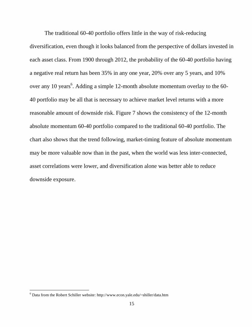
The traditional 60-40 portfolio offers little in the way of risk-reducing

diversification, even though it looks balanced from the perspective of dollars invested in

each asset class. From 1900 through 2012, the probability of the 60-40 portfolio having

a negative real return has been 35% in any one year, 20% over any 5 years, and 10%

over any 10 years6. Adding a simple 12-month absolute momentum overlay to the 60-

40 portfolio may be all that is necessary to achieve market level returns with a more

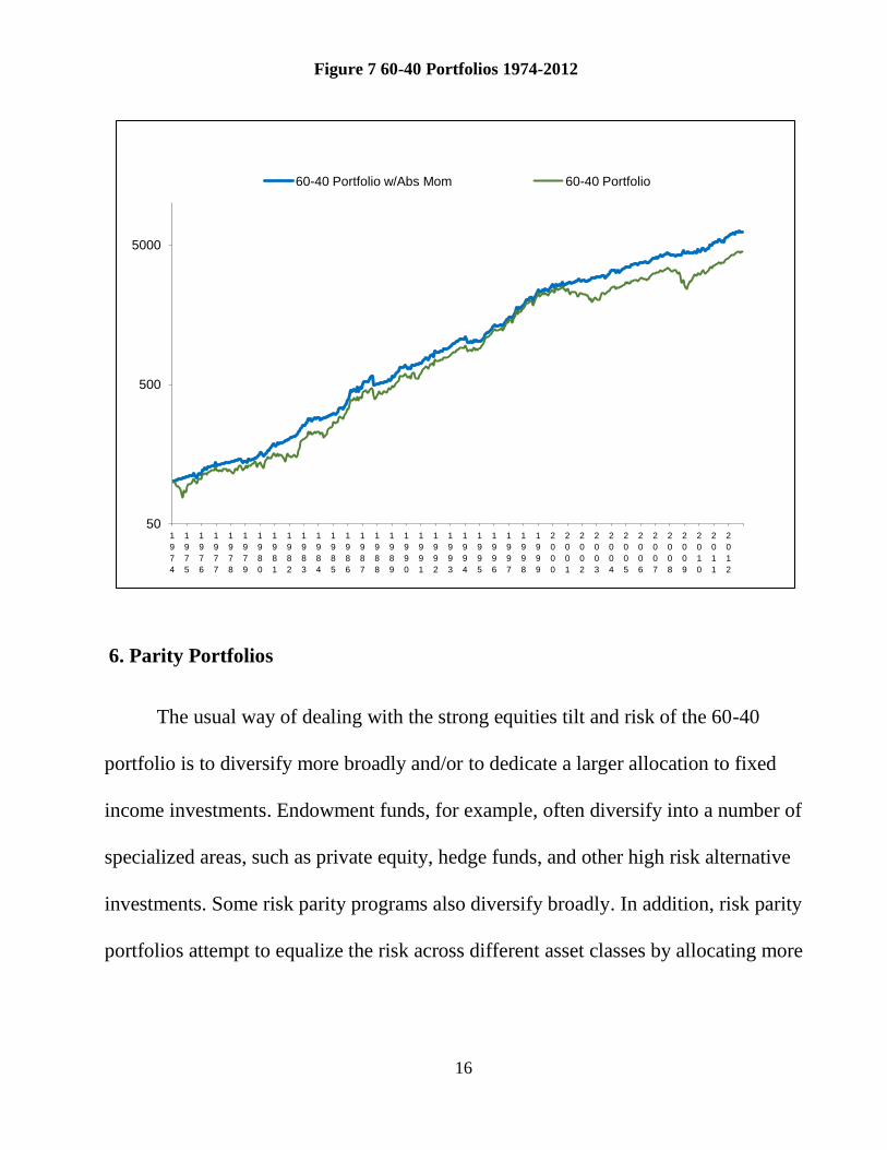
reasonable amount of downside risk. Figure 7 shows the consistency of the 12-month

absolute momentum 60-40 portfolio compared to the traditional 60-40 portfolio. The

chart also shows that the trend following, market-timing feature of absolute momentum

may be more valuable now than in the past, when the world was less inter-connected,

asset correlations were lower, and diversification alone was better able to reduce

downside exposure.

6 Data from the Robert Schiller website: http://www.econ.yale.edu/~shiller/data.htm

16

6. Parity Portfolios

The usual way of dealing with the strong equities tilt and risk of the 60-40

portfolio is to diversify more broadly and/or to dedicate a larger allocation to fixed

income investments. Endowment funds, for example, often diversify into a number of

specialized areas, such as private equity, hedge funds, and other high risk alternative

investments. Some risk parity programs also diversify broadly. In addition, risk parity

portfolios attempt to equalize the risk across different asset classes by allocating more

50

500

5000

1

9

7

4

1

9

7

5

1

9

7

6

1

9

7

7

1

9

7

8

1

9

7

9

1

9

8

0

1

9

8

1

1

9

8

2

1

9

8

3

1

9

8

4

1

9

8

5

1

9

8

6

1

9

8

7

1

9

8

8

1

9

8

9

1

9

9

0

1

9

9

1

1

9

9

2

1

9

9

3

1

9

9

4

1

9

9

5

1

9

9

6

1

9

9

7

1

9

9

8

1

9

9

9

2

0

0

0

2

0

0

1

2

0

0

2

2

0

0

3

2

0

0

4

2

0

0

5

2

0

0

6

2

0

0

7

2

0

0

8

2

0

0

9

2

0

1

0

2

0

1

1

2

0

1

2

60-40 Portfolio w/Abs Mom 60-40 Portfolio

Figure 7 60-40 Portfolios 1974-2012

17

to lower volatility assets. A stock-bond only portfolio, for example, would require at

least a 70% allocation to bonds in order to have equal risk from bonds and equities.

We can construct a simple, monthly-rebalanced risk parity portfolio and apply

12-month absolute momentum to it. Starting with the same MSCI US and long Treasury

bond indices used in our 60-40 portfolio, we add REITs, credit bonds, and gold, with an

equal weighting given to all. We use credit bonds to increase the low-volatility, fixed

income side of the portfolio. Credit bonds also diversify our fixed income allocation by

providing credit risk premium and less duration risk than long Treasuries. REITs give

exposure to real assets and equities. Gold has the highest volatility, and so represents

only 20% of the portfolio, whereas equities and fixed income make up the majority of

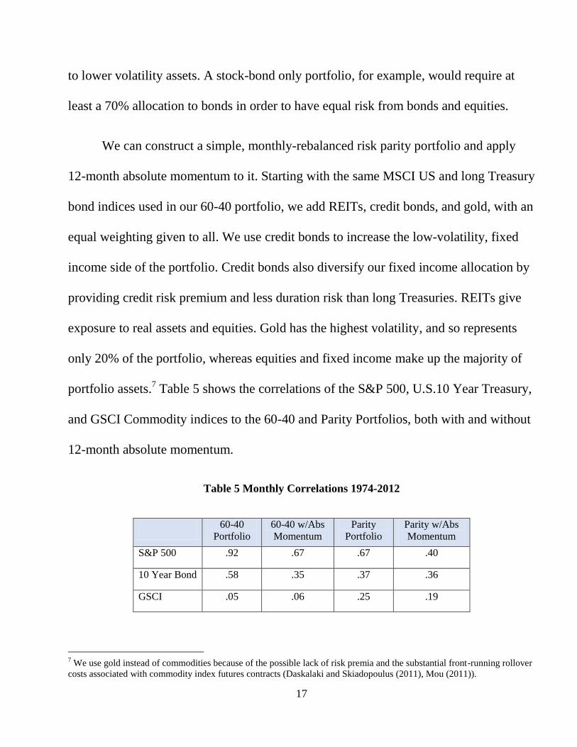
portfolio assets.7 Table 5 shows the correlations of the S&P 500, U.S.10 Year Treasury,

and GSCI Commodity indices to the 60-40 and Parity Portfolios, both with and without

12-month absolute momentum.

Table 5 Monthly Correlations 1974-2012

7 We use gold instead of commodities because of the possible lack of risk premia and the substantial front-running rollover

costs associated with commodity index futures contracts (Daskalaki and Skiadopoulus (2011), Mou (2011)).

60-40

Portfolio

60-40 w/Abs

Momentum

Parity

Portfolio

Parity w/Abs

Momentum

S&P 500 .92 .67 .67 .40

10 Year Bond .58 .35 .37 .36

GSCI .05 .06 .25 .19

18

Our Parity Portfolio with 12-month absolute momentum shows a modest and

nearly equal correlation to both stocks and bonds. Because of the downside risk

attenuation through absolute momentum, we have achieved risk parity while limiting

fixed income to only 40% of our assets. Having a well-balanced portfolio means that in

low growth and low inflation environments, gold and bonds may outperform and

sustain the portfolio, whereas equities and REITs may perform better under high

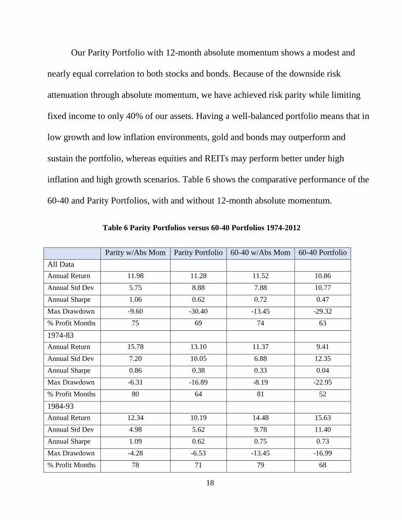
inflation and high growth scenarios. Table 6 shows the comparative performance of the

60-40 and Parity Portfolios, with and without 12-month absolute momentum.

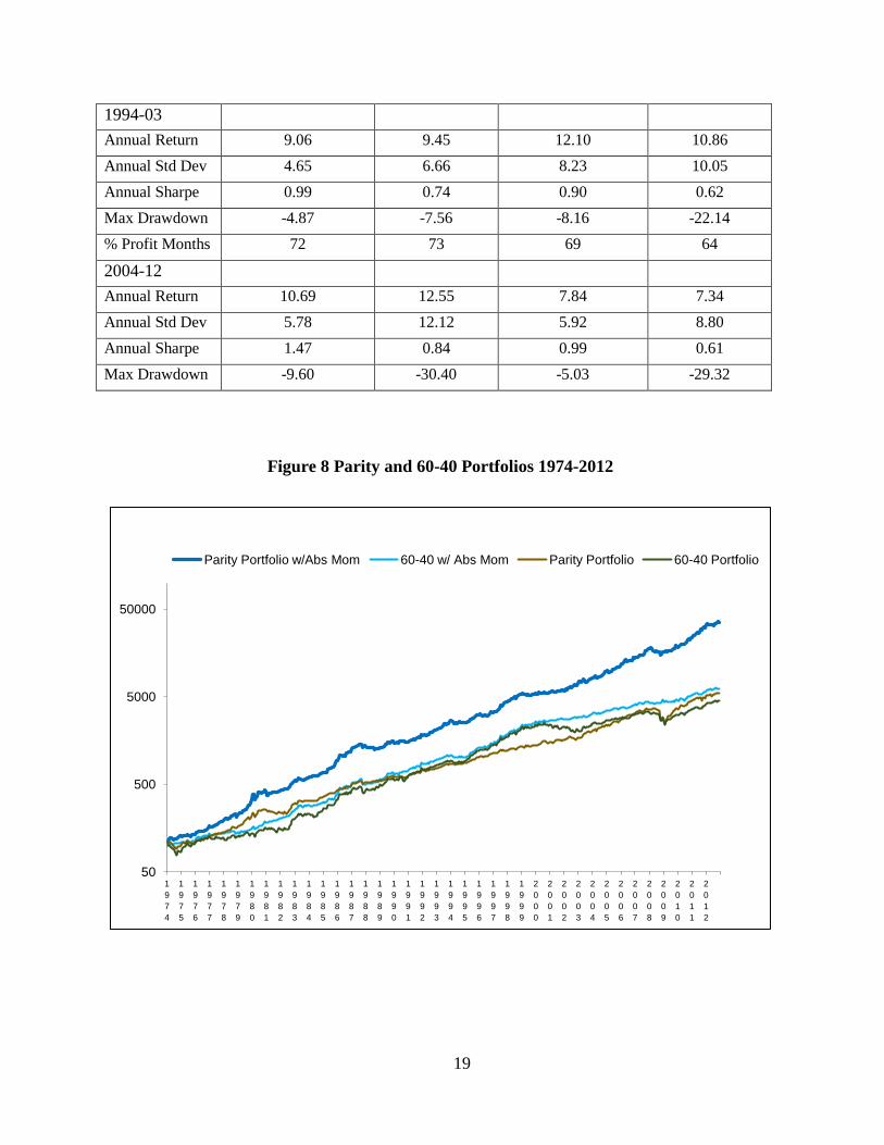
Table 6 Parity Portfolios versus 60-40 Portfolios 1974-2012

Parity w/Abs Mom Parity Portfolio 60-40 w/Abs Mom 60-40 Portfolio

All Data

Annual Return 11.98 11.28 11.52 10.86

Annual Std Dev 5.75 8.88 7.88 10.77

Annual Sharpe 1.06 0.62 0.72 0.47

Max Drawdown -9.60 -30.40 -13.45 -29.32

% Profit Months 75 69 74 63

1974-83

Annual Return 15.78 13.10 11.37 9.41

Annual Std Dev 7.20 10.05 6.88 12.35

Annual Sharpe 0.86 0.38 0.33 0.04

Max Drawdown -6.31 -16.89 -8.19 -22.95


1984-93

Annual Return 12.34 10.19 14.48 15.63

Annual Std Dev 4.98 5.62 9.78 11.40

Annual Sharpe 1.09 0.62 0.75 0.73

Max Drawdown -4.28 -6.53 -13.45 -16.99


19

1994-03

Annual Return 9.06 9.45 12.10 10.86

Annual Std Dev 4.65 6.66 8.23 10.05

Annual Sharpe 0.99 0.74 0.90 0.62

Max Drawdown -4.87 -7.56 -8.16 -22.14


2004-12

Annual Return 10.69 12.55 7.84 7.34

Annual Std Dev 5.78 12.12 5.92 8.80

Annual Sharpe 1.47 0.84 0.99 0.61

Max Drawdown -9.60 -30.40 -5.03 -29.32

50

500

5000

50000

1

9

7

4

1

9

7

5

1

9

7

6

1

9

7

7

1

9

7

8

1

9

7

9

1

9

8

0

1

9

8

1

1

9

8

2

1

9

8

3

1

9

8

4

1

9

8

5

1

9

8

6

1

9

8

7

1

9

8

8

1

9

8

9

1

9

9

0

1

9

9

1

1

9

9

2

1

9

9

3

1

9

9

4

1

9

9

5

1

9

9

6

1

9

9

7

1

9

9

8

1

9

9

9

2

0

0

0

2

0

0

1

2

0

0

2

2

0

0

3

2

0

0

4

2

0

0

5

2

0

0

6

2

0

0

7

2

0

0

8

2

0

0

9

2

0

1

0

2

0

1

1

2

0

1

2

Parity Portfolio w/Abs Mom 60-40 w/ Abs Mom Parity Portfolio 60-40 Portfolio

Figure 8 Parity and 60-40 Portfolios 1974-2012

20

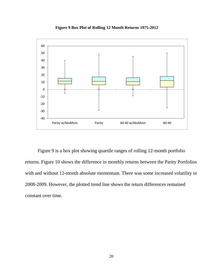
Figure 9 Box Plot of Rolling 12 Month Returns 1975-2012

Figure 9 is a box plot showing quartile ranges of rolling 12-month portfolio

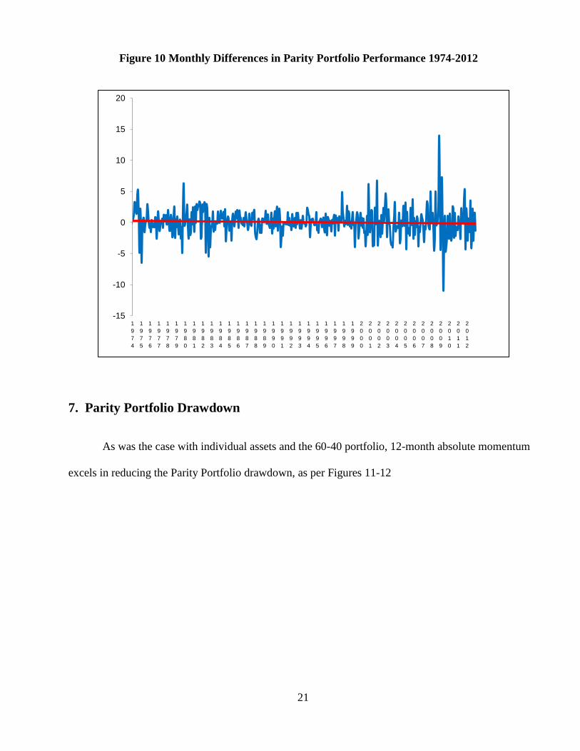
returns. Figure 10 shows the difference in monthly returns between the Parity Portfolios

with and without 12-month absolute momentum. There was some increased volatility in

2008-2009. However, the plotted trend line shows the return differences remained

constant over time.

-40

-30

-20

-10

0

10

20

30

40

50

60

Parity w/AbsMom Parity 60-40 w/AbsMom 60-40

21

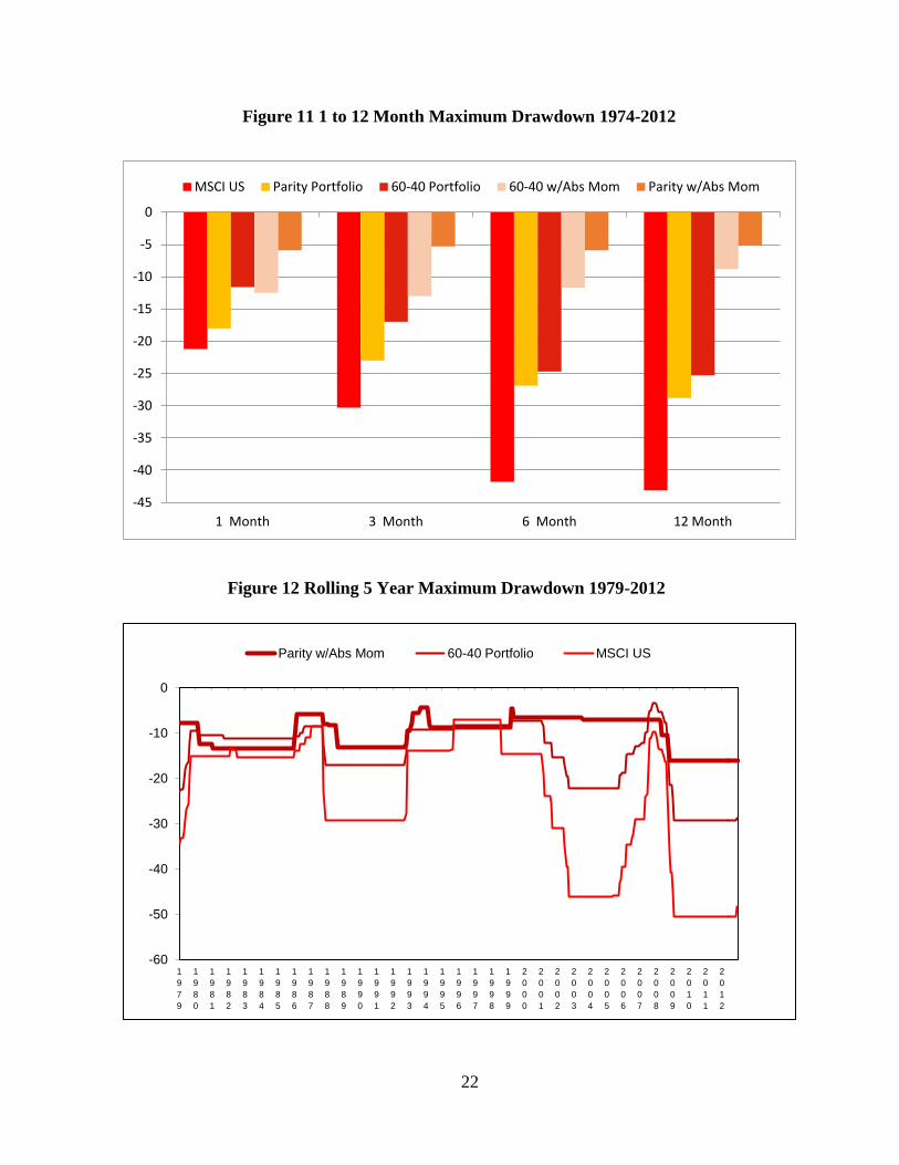
7. Parity Portfolio Drawdown

As was the case with individual assets and the 60-40 portfolio, 12-month absolute momentum

excels in reducing the Parity Portfolio drawdown, as per Figures 11-12

-15

-10

-5

0

5

10

15

20

1

9

7

4

1

9

7

5

1

9

7

6

1

9

7

7

1

9

7

8

1

9

7

9

1

9

8

0

1

9

8

1

1

9

8

2

1

9

8

3

1

9

8

4

1

9

8

5

1

9

8

6

1

9

8

7

1

9

8

8

1

9

8

9

1

9

9

0

1

9

9

1

1

9

9

2

1

9

9

3

1

9

9

4

1

9

9

5

1

9

9

6

1

9

9

7

1

9

9

8

1

9

9

9

2

0

0

0

2

0

0

1

2

0

0

2

2

0

0

3

2

0

0

4

2

0

0

5

2

0

0

6

2

0

0

7

2

0

0

8

2

0

0

9

2

0

1

0

2

0

1

1

2

0

1

2

Figure 10 Monthly Differences in Parity Portfolio Performance 1974-2012

22

-60

-50

-40

-30

-20

-10

0

1

9

7

9

1

9

8

0

1

9

8

1

1

9

8

2

1

9

8

3

1

9

8

4

1

9

8

5

1

9

8

6

1

9

8

7

1

9

8

8

1

9

8

9

1

9

9

0

1

9

9

1

1

9

9

2

1

9

9

3

1

9

9

4

1

9

9

5

1

9

9

6

1

9

9

7

1

9

9

8

1

9

9

9

2

0

0

0

2

0

0

1

2

0

0

2

2

0

0

3

2

0

0

4

2

0

0

5

2

0

0

6

2

0

0

7

2

0

0

8

2

0

0

9

2

0

1

0

2

0

1

1

2

0

1

2

Parity w/Abs Mom 60-40 Portfolio MSCI US

-45

-40

-35

-30

-25

-20

-15

-10

-5

0

1 Month 3 Month 6 Month 12 Month

MSCI US Parity Portfolio 60-40 Portfolio 60-40 w/Abs Mom Parity w/Abs Mom

Figure 12 Rolling 5 Year Maximum Drawdown 1979-2012

Figure 11 1 to 12 Month Maximum Drawdown 1974-2012

23

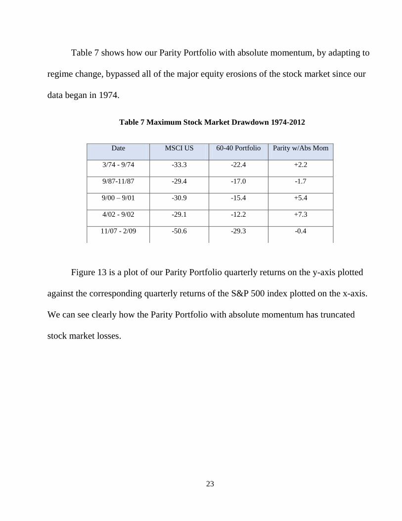
Table 7 shows how our Parity Portfolio with absolute momentum, by adapting to

regime change, bypassed all of the major equity erosions of the stock market since our

data began in 1974.

Table 7 Maximum Stock Market Drawdown 1974-2012

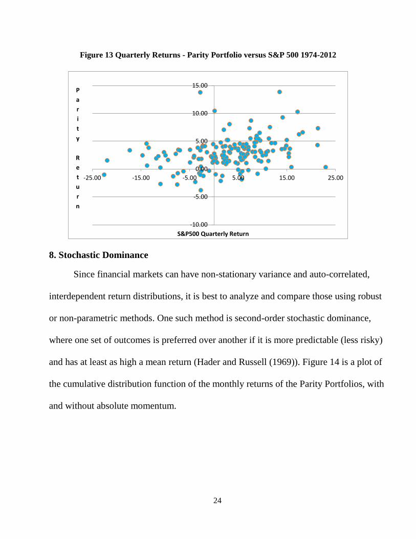
Figure 13 is a plot of our Parity Portfolio quarterly returns on the y-axis plotted

against the corresponding quarterly returns of the S&P 500 index plotted on the x-axis.

We can see clearly how the Parity Portfolio with absolute momentum has truncated

stock market losses.

Date MSCI US 60-40 Portfolio Parity w/Abs Mom

3/74 - 9/74 -33.3 -22.4 +2.2

9/87-11/87 -29.4 -17.0 -1.7

9/00 – 9/01 -30.9 -15.4 +5.4

4/02 - 9/02 -29.1 -12.2 +7.3

11/07 - 2/09 -50.6 -29.3 -0.4

24

8. Stochastic Dominance

Since financial markets can have non-stationary variance and auto-correlated,

interdependent return distributions, it is best to analyze and compare those using robust

or non-parametric methods. One such method is second-order stochastic dominance,

where one set of outcomes is preferred over another if it is more predictable (less risky)

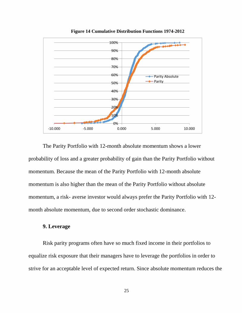
and has at least as high a mean return (Hader and Russell (1969)). Figure 14 is a plot of

the cumulative distribution function of the monthly returns of the Parity Portfolios, with

and without absolute momentum.

-10.00

-5.00

0.00

5.00

10.00

15.00

-25.00 -15.00 -5.00 5.00 15.00 25.00

P

a

r

i

t

y

R

e

t

u

r

n

S&P500 Quarterly Return

Figure 13 Quarterly Returns - Parity Portfolio versus S&P 500 1974-2012

25

Figure 14 Cumulative Distribution Functions 1974-2012

The Parity Portfolio with 12-month absolute momentum shows a lower

probability of loss and a greater probability of gain than the Parity Portfolio without

momentum. Because the mean of the Parity Portfolio with 12-month absolute

momentum is also higher than the mean of the Parity Portfolio without absolute

momentum, a risk- averse investor would always prefer the Parity Portfolio with 12-

month absolute momentum, due to second order stochastic dominance.

9. Leverage

Risk parity programs often have so much fixed income in their portfolios to

equalize risk exposure that their managers have to leverage the portfolios in order to

strive for an acceptable level of expected return. Since absolute momentum reduces the

0%

10%

20%

30%

40%

50%

60%

70%

80%

90%

100%

-10.000 -5.000 0.000 5.000 10.000

Parity Absolute Parity

26

volatility of our Parity Portfolio while, at the same, preserving equity level returns,

there is not the same need for leverage.

However, given the low expected drawdown of an absolute momentum Parity

Portfolio, one may still wish to use leverage in order to boost expected returns, as is

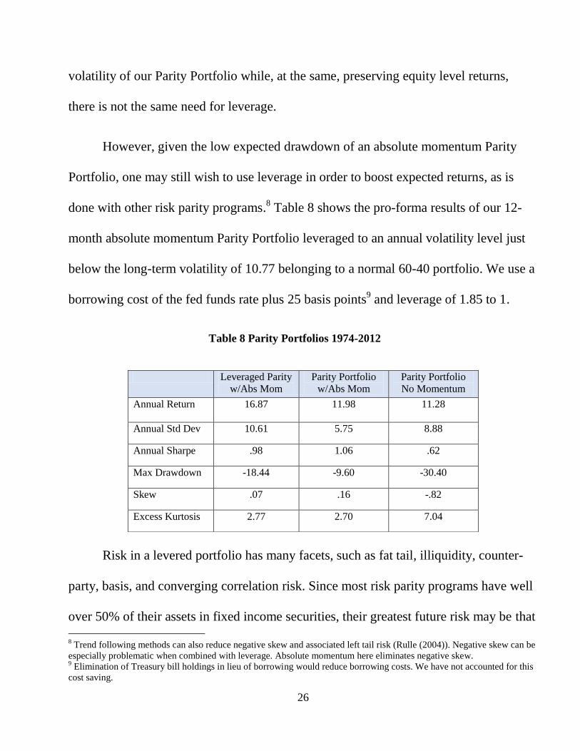
done with other risk parity programs.8 Table 8 shows the pro-forma results of our 12-

month absolute momentum Parity Portfolio leveraged to an annual volatility level just

below the long-term volatility of 10.77 belonging to a normal 60-40 portfolio. We use a

borrowing cost of the fed funds rate plus 25 basis points9 and leverage of 1.85 to 1.

Table 8 Parity Portfolios 1974-2012

Risk in a levered portfolio has many facets, such as fat tail, illiquidity, counter-

party, basis, and converging correlation risk. Since most risk parity programs have well

over 50% of their assets in fixed income securities, their greatest future risk may be that

8 Trend following methods can also reduce negative skew and associated left tail risk (Rulle (2004)). Negative skew can be

especially problematic when combined with leverage. Absolute momentum here eliminates negative skew. 9 Elimination of Treasury bill holdings in lieu of borrowing would reduce borrowing costs. We have not accounted for this

cost saving.

Leveraged Parity

w/Abs Mom

Parity Portfolio

w/Abs Mom

Parity Portfolio

No Momentum

Annual Return 16.87

11.98 11.28

Annual Std Dev 10.61 5.75 8.88

Annual Sharpe .98 1.06 .62

Max Drawdown -18.44 -9.60 -30.40

Skew .07 .16 -.82

Excess Kurtosis 2.77 2.70 7.04

27

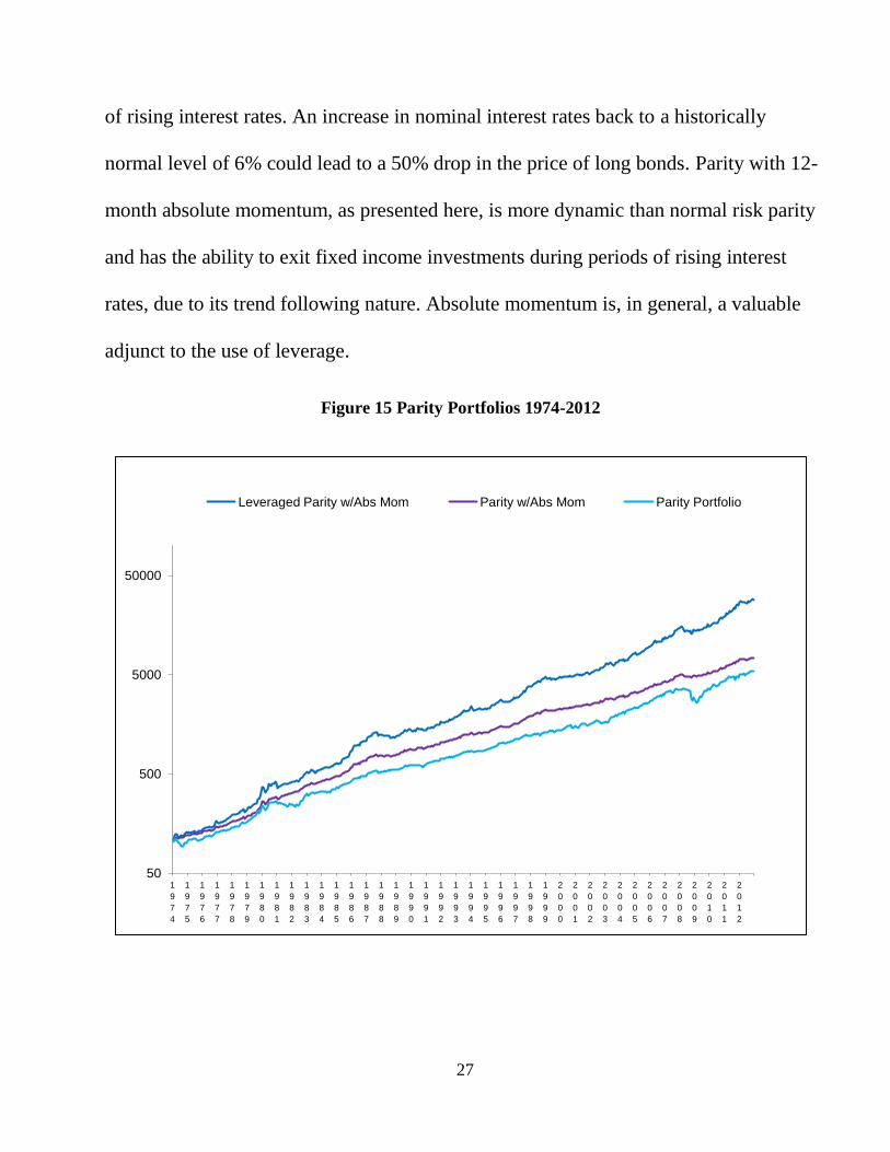
of rising interest rates. An increase in nominal interest rates back to a historically

normal level of 6% could lead to a 50% drop in the price of long bonds. Parity with 12-

month absolute momentum, as presented here, is more dynamic than normal risk parity

and has the ability to exit fixed income investments during periods of rising interest

rates, due to its trend following nature. Absolute momentum is, in general, a valuable

adjunct to the use of leverage.

50

500

5000

50000

1

9

7

4

1

9

7

5

1

9

7

6

1

9

7

7

1

9

7

8

1

9

7

9

1

9

8

0

1

9

8

1

1

9

8

2

1

9

8

3

1

9

8

4

1

9

8

5

1

9

8

6

1

9

8

7

1

9

8

8

1

9

8

9

1

9

9

0

1

9

9

1

1

9

9

2

1

9

9

3

1

9

9

4

1

9

9

5

1

9

9

6

1

9

9

7

1

9

9

8

1

9

9

9

2

0

0

0

2

0

0

1

2

0

0

2

2

0

0

3

2

0

0

4

2

0

0

5

2

0

0

6

2

0

0

7

2

0

0

8

2

0

0

9

2

0

1

0

2

0

1

1

2

0

1

2

Leveraged Parity w/Abs Mom Parity w/Abs Mom Parity Portfolio

Figure 15 Parity Portfolios 1974-2012

28

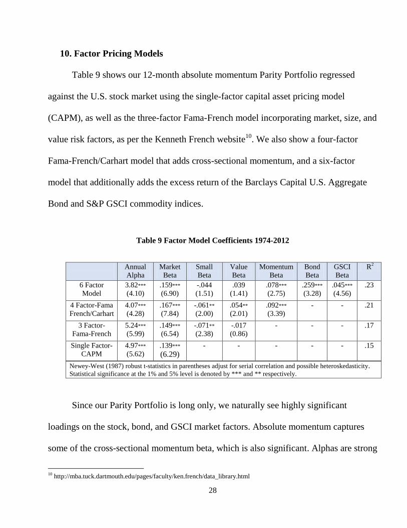
10. Factor Pricing Models

Table 9 shows our 12-month absolute momentum Parity Portfolio regressed

against the U.S. stock market using the single-factor capital asset pricing model

(CAPM), as well as the three-factor Fama-French model incorporating market, size, and

value risk factors, as per the Kenneth French website10

. We also show a four-factor

Fama-French/Carhart model that adds cross-sectional momentum, and a six-factor

model that additionally adds the excess return of the Barclays Capital U.S. Aggregate

Bond and S&P GSCI commodity indices.

Table 9 Factor Model Coefficients 1974-2012

Newey-West (1987) robust t-statistics in parentheses adjust for serial correlation and possible heteroskedasticity. Statistical significance at the 1% and 5% level is denoted by *** and ** respectively.

Since our Parity Portfolio is long only, we naturally see highly significant

loadings on the stock, bond, and GSCI market factors. Absolute momentum captures

some of the cross-sectional momentum beta, which is also significant. Alphas are strong

10

http://mba.tuck.dartmouth.edu/pages/faculty/ken.french/data_library.html

Annual

Alpha

Market

Beta

Small

Beta

Value

Beta

Momentum

Beta

Bond

Beta

GSCI

Beta

R2

6 Factor

Model

3.82***

(4.10)

.159***

(6.90)

-.044

(1.51)

.039

(1.41)

.078***

(2.75)

.259***

(3.28)

.045***

(4.56)

.23

4 Factor-Fama

French/Carhart

4.07***

(4.28)

.167***

(7.84)

-.061**

(2.00)

.054**

(2.01)

.092***

(3.39)

- - .21

3 Factor-

Fama-French

5.24***

(5.99)

.149***

(6.54)

-.071**

(2.38)

-.017

(0.86)

- - - .17

Single Factor-

CAPM

4.97***

(5.62)

.139***

(6.29) - - - - - .15

29

and highly significant under all four pricing models. Our Parity Portfolio with 12-month

absolute momentum provides substantial and significant alphas according to all four

models.

11. Conclusions

Cowles and Jones first presented 12-month momentum to the public in 1937. It has

held up remarkably well ever since. Relative strength momentum, looking at

performance against one's peers, has attracted the most attention from researchers and

investors. Yet it is only a secondary way of looking at price strength. Absolute

momentum, measuring an asset's performance with respect to its own past, is a more

direct way of looking at and utilizing market trends to determine price continuation.

Trend determination through absolute momentum can help one navigate downside

risk, take advantage of regime persistence, and achieve extraordinary risk-adjusted

returns. Absolute momentum, as used here, is a simple rule-based approach that is easy

to implement. One needs only see if returns relative to Treasury bills have been up or

down for the preceding year.

We have seen how 12-month absolute momentum can help improve the reward-to-

risk characteristics of a broad range of individual investments. Absolute momentum

also has considerable value as a tactical overlay to multi-asset portfolios, where it has

many potential uses. Absolute momentum can enhance the expected return and reduce

the expected drawdown of core portfolios, as we have shown in this paper. It can help

30

investors with basic stock/bond allocations, such as the 60-40 mix, meet their

investment objectives without resorting to leverage, riskier assets such as hedge funds

and private placements, and complex portfolio constructs that rely heavily on the use of

non-stationary correlation and covariance.

Absolute momentum can be an attractive alternative to option overwriting by

retaining more of the potential for upside appreciation, while at the same time providing

greater downside protection. Absolute momentum can similarly be an attractive

alternative to costly tail risk hedging. It can reduce or eliminate diminishing returns

from over-aggressive diversification. If one wishes to achieve higher returns by using

riskier assets or by leveraging a portfolio, then 12- month absolute momentum can

make that more viable by truncating expected drawdown.

Despite its many possible uses, absolute momentum has yet to attract the attention

it deserves as an attractive investment strategy and risk management tool. We have

developed applications for, variations of, and enhancements to 12- month absolute

momentum that go beyond the scope of this introductory paper. Yet all investors would

do well to become familiar with absolute momentum, since, even in its simplest form as

presented here, absolute momentum can be an attractive stand-alone strategy, or a

powerful tactical overlay for improving the risk-adjusted performance of most any asset

or portfolio.

31

References

Antonacci, Gary, 2013, "Risk Premia Harvesting Through Dual Momentum," working

paper, Portfolio Management Associates, LLC, working paper

Asness, Clifford S., Tobias J. Moskowitz, and Lasse J. Pedersen, 2012, “Value and

Momentum Everywhere,” Journal of Finance, forthcoming

Baltas, Akindynos-Nikolaos and Robert Kosowski, 2012, "Improving Time Series

Momentum Strategies: The Role of Trading Signals and Volatility Estimators," working

paper

Barberis, Nicholas, Andrei Shleifer, and Robert Vishny, 1998, "A Model of Investor

Sentiment," Journal of Financial Economics 49, 307–343

Blitz, David C and Pim Van Vliet, 2008, "Global Tactical Cross-Asset Allocation:

Applying Value and Momentum Across Asset Classes," Journal of Portfolio

Management 35(1), 23-38

Brock, William, Josef Lakonishok, and Blake LeBaron, 1992, "Simple Technical

Trading Rules and the Stochastic Properties of Stock Returns," Journal of Finance 47,

1731–1764

Chabot, Benjamin R., Eric Ghysels, and Ravi Jagannathan, 2009, “Price Momentum in

Stocks: Insights from Victorian Age Data,” working paper, National Bureau of

Economic Research

Cowles, Alfred III and Herbert E. Jones, 1937, "Some A Priori Probabilities in Stock

Market Action," Econometrica 5(3), 280-294

Daniel, Kent, David Hirshleifer, and Avanidhar Subrahmanyam, 1998, "Investor

Psychology and Security Market Under-and Over-Reactions." Journal of Finance 53,

1839–1886

Daskalaki, Charoula and George S Skiadopoulus, 2011, "Should Investors Include

Commodities in Their Portfolios After All? New Evidence," Journal of Banking and

Finance 35 (10), 2606-2626

Frazzini, Andrea, 2006, "The Disposition Effect and Underreaction to News,"

Journal of Finance 61, 2017-2046

32

Garleanu, Nicolae and Lasse H Pedersen, 2007, “Liquidity and Risk Management,” The

American Economic Review 97, 193-197

Grundy, Bruce D and J Spencer Martin, 2001, “Understanding the Nature of the Risks

and the Sources of the Rewards to Momentum Investing,” Review of Financial Studies

14, 29-78

Hader, Josef and William R Russell, 1969, "Rules for Ordering Uncertain Prospects,"

The American Economic Review 59(1), 25-34.

Han, Yufeng, Ke Yang, and Guofo Zhou, 2011, "A New Anomaly: The Cross-Sectional

Profitability of Technical Analysis," working paper

Hong, Harrison and Jeremy Stein, 1999, "A Unified Theory of Underreaction,

Momentum Trading, and Overreaction in Asset Markets," Journal of Finance 54, 2143-

2184

Hurst, Brian, Yao Hua Ooi, and Lasse H Pedersen, 2012, "A Century of Evidence on

Trend-Following Investing," AQR Capital Management, LLC

Jegadeesh, Narasimhan and Sheridan Titman, 1993, “Returns to Buying Winners and

Selling Losers: Implications for Stock Market Efficiency,” Journal of Finance 48, 65-

91

Jegadeesh, Narasimhan and Sheridan Titman, 2001, "Profitability of Momentum

Strategies: An Evaluation of Alternative Explanations," Journal of Finance 56(2), 699–

720

Lo, Andrew W., Harry Mamaysky, and Jiang Wang, 2000, "Foundations of Technical

Analysis: Computational Algorithms, Statistical Inference, and Empirical

Implementation," Journal of Finance 55, 1705–1770

Mou, Ziqun, 2011, "Limits to Arbitrage and Commodity Index Investment: Front-

Running the Goldman Yield," working paper

Moskowitz, Tobias J., Yao Hua Ooi, and Lasse Heje Pedersen, 2012, "Time Series

Momentum," Journal of Financial Economics 104, 228-250

Newey, Whitney K. and Kenneth D. West, 1987, "A Simple, Positive Semi-Definite,

33

Heteroskedasticity and Autocorrelation Consistent Covariance Matrix," Econometrica

55(3),

703–708

Rulle, Michael, 2004, "Trend Following: Performance, Risk, and Correlation

Characteristics," Grantham Capital Management

Tversky, Amos and Daniel Kahneman, 1974, "Judgment Under Uncertainty: Heuristics

and Biases," Science 185, 1124-1131

Zhu, Yingzi and Guofu Zhou, 2009, "Technical Analysis: An Asset Allocation

Perspective on the Use of Moving Averages," Journal of Financial Economics 92, 519-

544

absolute momentum: a simple rule-based strategy and ... · pdf file1 absolute momentum: a...

Documents