aalborg universitet learning bayesian networks with …vbn.aau.dk/files/1278250/phd11.pdflearning...
TRANSCRIPT

Aalborg Universitet
Learning Bayesian Networks with Mixed Variables
Bøttcher, Susanne Gammelgaard
Publication date:2005
Document VersionPublisher's PDF, also known as Version of record
Link to publication from Aalborg University
Citation for published version (APA):Bøttcher, S. G. (2005). Learning Bayesian Networks with Mixed Variables. Ph.D. Report Series, No. 11
General rightsCopyright and moral rights for the publications made accessible in the public portal are retained by the authors and/or other copyright ownersand it is a condition of accessing publications that users recognise and abide by the legal requirements associated with these rights.
? Users may download and print one copy of any publication from the public portal for the purpose of private study or research. ? You may not further distribute the material or use it for any profit-making activity or commercial gain ? You may freely distribute the URL identifying the publication in the public portal ?
Take down policyIf you believe that this document breaches copyright please contact us at [email protected] providing details, and we will remove access tothe work immediately and investigate your claim.
Downloaded from vbn.aau.dk on: juni 28, 2018

Learning Bayesian Networkswith Mixed Variables
Susanne Gammelgaard Bøttcher
Ph.D. Thesis
2004
AALBORG UNIVERSITY
Department of Mathematical Sciences


Preface
This thesis is the result of my Ph.D. study at the Department of MathematicalSciences, Aalborg University, Denmark. The work has mainlybeen founded byAalborg University, but also in parts by the ESPRIT project P29105 (BaKE) andby Novo Nordisk A/S.
The thesis concerns learning Bayesian networks with both discrete and contin-uous variables and is based on the following four papers:
I. Learning Conditional Gaussian Networks.
II. deal: A Package for Learning Bayesian Networks.
III. Prediction of the Insulin Sensitivity Index using Bayesian Networks.
IV. Learning Dynamic Bayesian Networks with Mixed Variables.
Many of the results in Paper I are published in Bøttcher (2001). Paper II ispublished in Bøttcher and Dethlefsen (2003a). The developed software pack-age,deal, is written inR (R Development Core Team 2003) and can be down-loaded from the ComprehensiveR Archive Network (CRAN)http://cran.R-project.org/. Paper II and Paper III are written together with ClausDethlefsen, Aalborg University.
The individual papers are self-contained with an individual bibliography andfigure, table and equation numbering. Parts and bits therefore appear in morethan one paper. A basic understanding of the results in Paper1 is though anadvantage in reading the other papers. Those who are not familiar with Bayesiannetworks in general, might consult introductory books suchas Jensen (1996)and Cowell, Dawid, Lauritzen and Spiegelhalter (1999).
iii

iv PREFACE
I am much indebted to my supervisor Steffen L. Lauritzen for inspiring dis-cussions and for many valuable comments. Also thanks to Søren Lundbye-Christensen who has always taken the time to help me, when I had some ques-tions.
I owe a special thanks to Claus Dethlefsen for an inspiring collaboration and forsharing his expertise within statistical programming withme.
Part of the work is based on data provided by Torben Hansen, Novo NordiskA/S. Thanks for letting us use these data.
From September 1999 to November 1999 I visited the Fields Institute in Toronto,Canada, as a participant in the research program "Causal Interpretation andIdentification of Conditional Independence Structures". Iwish to thank all thepeople there for a memorable stay.
Acknowledgements also go to my colleagues at the Departmentof Mathemati-cal Sciences for providing a nice working environment and especially to E. Su-sanne Christensen, who has been my mentor and one of my best friends duringthe years I have worked at the department.
Special thanks go to my colleagues and very dear friends Malene, Kim andClaus. We always have a lot of fun together and we are also their for each otherduring the hard times.
Both my parents and my in-laws have been very supportive during this studyand that has meant a lot to me, so a word of thanks also goes to them.
All my thanks go to my two sons, Johannes and Magnus, for reminding me ofthe things that are the most important in life.
Finally, I would like to thank my husband Peter for his invaluable support andendless encouragement during my Ph.D. study. Also thanks for caring for Jo-hannes and Magnus during my sometimes long work hours. It wasthe thoughtof having more time to spent with the three of you that finally made me finishthis thesis.
Aalborg, Denmark, March 2004 Susanne Gammelgaard Bøttcher

Summary
The main topic of this thesis is learning Bayesian networks with discrete andcontinuous variables.
A Bayesian network is a directed acyclic graph that encodes the joint probabilitydistribution for a set of random variables. The nodes in the graph representthe random variables and missing arrows between the nodes, specify propertiesof conditional independence between the variables. It consists of two parts,a knowledge base and an inference engine for handling this knowledge. Thisthesis relies on already developed methods for inference and concentrate onconstructing the knowledge base.
When constructing the knowledge base, there are two things to consider, namelylearning the graphical structure and learning the parameters in the probabilitydistributions. In this thesis, the focus is on learning Bayesian networks, wherethe joint probability distribution is conditional Gaussian. To learn the parame-ters, conjugate Bayesian analysis is used and parameter independence and com-plete data are assumed. To learn the graphical structure, network scores forthe different structures under evaluation, are calculatedand used to discriminatebetween the structures. To calculate these scores, the prior distribution for theparameters for each network under evaluation, must be specified. An automatedprocedure for doing this is developed. With this procedure,the parameter priorsfor all possible networks are deduced from marginal priors calculated from animaginary database.
Bayes factors to be used when searching for structures with high network score,are also studied. To reduce the search complexity, classes of models are iden-tified for which the Bayes factor for testing an arrow betweenthe same twovariables, is the same.
v

vi SUMMARY
To be able to use the methods in practice, a software package called deal,written inR, is developed. The package includes procedures for definingpriors,estimating parameters, calculating network scores, performing heuristic searchas well as simulating data sets with a given dependency structure.
To illustrate the Bayesian learning procedure, a dataset from a study concern-ing the insulin sensitivity index, is analyzed. The insulinsensitivity index isan index that can be used in assessing the risk of developing type 2 diabetes.Interest is in developing a method to determine the index from measurementsof glucose and insulin concentrations in plasma sampled subsequently after anglucose intake. As the dependency relations between the glucose and insulinmeasurements are complicated, it is proposed to use Bayesian networks. Theconclusion is that the insulin sensitivity index for a non-diabetic glucose tol-erant subject can be predicted from the glucose and insulin measurements, thegender and the body mass index, using Bayesian networks.
Finally, dynamic Bayesian networks with mixed variables are studied. A dy-namic Bayesian network is just a simple extension of an ordinary Bayesiannetwork and is applied in the modeling of time series. It is shown how themethods developed for learning Bayesian networks with mixed variables, canbe extended to use for learning dynamic Bayesian networks with mixed vari-ables. As the Markov order of a times series is not always known, it is alsoshown how to learn this order.

Summary in Danish – sammendrag
Denne afhandling omhandler konstruktion (indlæring) af bayesianske netværkmed diskrete og kontinuerte variable.
Et bayesiansk netværk er en orienteret graf uden kredse, derbeskriver den si-multane sandsynlighedsfordeling for en mængde af stokastiske variable. Knu-derne i grafen repræsenter de stokastiske variable og manglende pile imellemknuderne repræsenterer betingede uafhængighedsantagelser. Et bayesiansk net-værk består af to dele, en vidensbase og en inferensmaskine til at håndteredenne viden. Denne afhandling bruger allerede udviklede metoder til inferensog fokuserer på at konstruere vidensbasen.
Konstruktionen af vidensbasen kan deles op i to dele, nemligselektion af dengrafiske struktur og estimation af parametrene i sandsynlighedsfordelingerne.I denne afhandling fokuseres der på bayesianske netværk, hvor den simultanesandsynlighedsfordeling er betinget gaussisk. Til parameter estimation brugeskonjugeret bayesiansk analyse og det antages, at parametrene er uafhængige ogat data er fuldstændige.
Til selektion af den grafiske struktur beregnes et mål for hvor godt en givenstruktur beskriver data, i afhandlingen kaldet for en netværksscore. Netværks-scoren beregnes for alle de strukturer, der tages i betragtning og bruges såledestil at diskriminere imellem de forskellige strukturer.
For at kunne beregne disse netværksscorer skal man kende apriori fordelingenfor parametrene i alle de betragtede netværk. En automatiskprocedure til at de-ducere disse apriori fordelinger fra marginale apriori fordelinger, beregnet fra enimaginær database, udvikles. Desuden studeres bayes faktorer, da disse bruges iforskellige søge strategier til søgning efter netværk med høj netværksscore. Forat reducere søge kompleksiteten identificeres klasser af modeller, hvor bayes
vii

viii SUMMARY IN DANISH – SAMMENDRAG
faktoren til at teste en pil mellem de samme to variable, er den samme.
For at kunne bruge de udviklede metoder i praksis, er et software program,kaldetdeal, udviklet. Pakken, som er skrevet tilR, inkluderer procedurertil at definere apriori fordelinger, estimere parametre, beregne netværksscorer,søge efter netværk med høj netværksscore og simulerer datasæt med en givenafhængighedsstruktur.
Til illustration af den bayesianske indlæringsprocedure analyseres et datasætfra et studie, der omhandler insulin sensitivitets indekset. Insulin sensitivitetsindekset er et indeks, der kan bruges til at vurdere risikoenfor at udvikle type2 diabetes. Formålet med studiet er at udvikle en metode, derkan bestemmedette indeks ud fra gentagne målinger af glukose og insulin koncentrationerne iplasma efter et glukose indtag. Da afhængighedsstrukturenmellem glukose oginsulin målingerne er kompleks, bruges bayesianske netværk til at repræsenteredisse afhængigheder. Konklusionen er at insulin sensitivitets indekset for ikke-diabetiske glukose tolerante individer, kan predikteres fra glukose og insulinmålingerne, kønnet og body mass indekset, ved at bruge bayesianske netværk.
Til sidst i afhandlingen studeres dynamiske bayesianske netværk med bland-ede variable. Et dynamisk bayesiansk netværk er en simpel udvidelse af desædvanlige bayesianske netværk og anvendes til modellering af tidsrække data.Det vises hvordan de metoder, der er udviklet til indlæring af de sædvanligebayesianske netværk med blandede variable, kan udvides, såde kan anvendestil indlæring af dynamiske bayesianske netværk med blandede variable. DaMarkov ordenen af en tidsrække ikke altid er kendt, vises detogså, hvordanman kan indlære denne orden.

Contents
Preface iii
Summary v
Summary in Danish – sammendrag vii
Introduction 1
Paper I. Learning Conditional Gaussian Networks 111 Introduction . . . . . . . . . . . . . . . . . . . . . . . . . . . . 132 Bayesian Networks . . . . . . . . . . . . . . . . . . . . . . . . 143 Bayesian Networks for Mixed Variables . . . . . . . . . . . . . 154 Learning the Parameters in a CG Network . . . . . . . . . . . . 175 Learning the Structure of a CG Network . . . . . . . . . . . . . 236 The Master Prior Procedure . . . . . . . . . . . . . . . . . . . . 267 Local Masters for Mixed Networks . . . . . . . . . . . . . . . . 318 Model Search . . . . . . . . . . . . . . . . . . . . . . . . . . . 349 Example . . . . . . . . . . . . . . . . . . . . . . . . . . . . . . 41
Paper II. deal: A Package for Learning Bayesian Networks 571 Introduction . . . . . . . . . . . . . . . . . . . . . . . . . . . . 592 Bayesian Networks . . . . . . . . . . . . . . . . . . . . . . . . 613 Data Structure . . . . . . . . . . . . . . . . . . . . . . . . . . . 624 Specification of a Bayesian Network . . . . . . . . . . . . . . . 635 Parameter Learning . . . . . . . . . . . . . . . . . . . . . . . . 676 Learning the Structure . . . . . . . . . . . . . . . . . . . . . . 737 Hugin Interface . . . . . . . . . . . . . . . . . . . . . . . . . . 788 Example . . . . . . . . . . . . . . . . . . . . . . . . . . . . . . 799 Discussion and Future Work . . . . . . . . . . . . . . . . . . . 8210 Manual Pages fordeal . . . . . . . . . . . . . . . . . . . . . . 84
ix

X CONTENTS
Paper III. Prediction of the Insulin Sensitivity Index using BayesianNetworks 1071 Introduction . . . . . . . . . . . . . . . . . . . . . . . . . . . . 1092 Data . . . . . . . . . . . . . . . . . . . . . . . . . . . . . . . . 1103 Bayesian Networks . . . . . . . . . . . . . . . . . . . . . . . . 1114 Inference . . . . . . . . . . . . . . . . . . . . . . . . . . . . . 1135 Results . . . . . . . . . . . . . . . . . . . . . . . . . . . . . . . 1156 Discussion . . . . . . . . . . . . . . . . . . . . . . . . . . . . . 124
Paper IV. Learning Dynamic Bayesian Networks with Mixed Variables1271 Introduction . . . . . . . . . . . . . . . . . . . . . . . . . . . . 1292 Dynamic Bayesian Networks . . . . . . . . . . . . . . . . . . . 1303 Dynamic Bayesian Networks for Mixed Variables . . . . . . . . 1344 Examples of DBNs . . . . . . . . . . . . . . . . . . . . . . . . 1375 Learning DBNs with Mixed Variables . . . . . . . . . . . . . . 1406 Specifying Prior Distributions . . . . . . . . . . . . . . . . . . 1497 Example . . . . . . . . . . . . . . . . . . . . . . . . . . . . . . 152

Introduction
The main focus of this Ph.D. thesis is to develop statisticalmethods for learningBayesian networks with mixed variables. To be able to use these methods inpractice, the software packagedeal is developed. Besides, the methods areextended to use for dynamic Bayesian networks.
Background
Bayesian networks was developed in the late 80’s by Pearl (1988) and Lauritzenand Spiegelhalter (1988). For terminology and theoreticalaspects, see Lauritzen(1996), Jensen (1996) and Cowell et al. (1999) among others.
A Bayesian network is a directed acyclic graph that encodes the joint probabilitydistribution for a set of random variables. The nodes in the graph represent therandom variables and missing arrows between the nodes, specify properties ofconditional independence between the variables.
A Bayesian network consists of two parts, a knowledge base and an inferenceengine for handling this knowledge. Generally, inference is computationallyheavy as it involves calculating huge joint distributions,especially if there aremany variables in the network. Therefore efficient methods of implementingBayes’ theorem are being used. These implementations uses the fact that thethe joint probability distribution of all the variables in anetwork, factorizes ac-cording to the structure of the graph. The distributions of interest can then befound by a series of local computations, involving only someof the variables ata time, seee.g.Cowell et al. (1999) for a thorough treatment of these methods.The methods are implemented ine.g. Hugin (http://www.hugin.com).Bayesian networks are therefore suitable for problems where the variables ex-hibit a complicated dependency structure. See Lauritzen (2003) for a recentoverview over different applications.
1

2 INTRODUCTION
In this thesis, we will rely on already developed methods forinference and con-centrate on constructing the knowledge base. The work is documented throughfour papers, which will be described in the following.
Paper I. Learning Conditional Gaussian Networks
When constructing the knowledge base there are two things toconsider, namelyspecifying the graphical structure and specifying the probability distributions.Paper I addresses these issues for Bayesian networks with mixed variables.
In this paper, the focus is on learning Bayesian networks, where the joint prob-ability distribution is conditional Gaussian. For an introductory text on learningBayesian networks, see Heckerman (1999). To learn the parameters in the lo-cal probability distributions, conjugate Bayesian analysis is used. As conjugatelocal priors, the Dirichlet distribution is applied for discrete variables and theGaussian-inverse gamma distribution is applied for continuous variables, givena configuration of the discrete parents. We assume parameterindependence andcomplete data. To learn the graphical structure, network scores for the differentstructures under evaluation, are calculated and these scores are used to discrim-inate between the structures. To calculate these scores, the prior distributionfor the parameters, for each network under evaluation, mustbe specified. InHeckerman, Geiger and Chickering (1995) and Geiger and Heckerman (1994)an automated procedure for doing this in respectively the purely discrete caseand the purely continuous case, is developed. Their work is based on principlesof likelihood equivalence, parameter modularity, and parameter independence.It leads to a method where the parameter priors for all possible networks, arededuced from one joint prior distribution, in this thesis called a master priordistribution.
In Paper I, we build on their results and develop a method, which can be usedon networks with mixed variables. If used on networks with only discrete vari-ables or only continuous variables, it coincides with the methods developed inin respectively Heckerman et al. (1995) and Geiger and Heckerman (1994).
If the number of random variables in a network is large, it is computationallyinfeasible to calculate the network score for all the possible structures. There-fore different methods for searching for structures with high network score, arebeing used, seee.g. Cooper and Herskovits (1992). Many of these methodsuse Bayes factors as a way of comparing the network scores fortwo differentmodels. We therefore study Bayes factors for mixed networks. To reduce thesearch complexity, classes of models are identified for which the Bayes factor

INTRODUCTION 3
for testing an arrow between the same two variables, is the same.
Finally, an analysis of a simple example illustrates the developed methods andis also used for showing how the strength of the prior parameter distributionaffects the result of the analysis.
Paper II. deal: A Package for Learning Bayesian Networks
To be able to use the methods presented in Paper I in practice,we have de-veloped a software package calleddeal, written in R (R Development CoreTeam 2003).
In particular, the package includes procedures for definingpriors, estimatingparameters, calculating network scores, performing heuristic search as wellas simulating data sets with a given dependency structure. The package canbe downloaded from the ComprehensiveR Archive Network (CRAN)http://cran.R-project.org/ and may be used under the terms of the GNUGeneral Public License Version 2.
The package supports transfer of the learned network to Hugin (http://www.hugin.com). The Hugin graphical user interface (GUI) can then be used forfurther inference in this network. Besides,deal adds functionality toR, so thatBayesian networks can be used in conjunction with other statistical methodsavailable inR for analyzing data. In particular,deal is part of the gR project,which is a newly initiated workgroup with the aim of developing proceduresin R for supporting data analysis with graphical models, seehttp://www.r-project.org/gR.
Paper III. Prediction of the Insulin Sensitivity Index using BayesianNetworks
To illustrate the Bayesian learning procedure, we have in Paper III analyzed adataset collected by Torben Hansen, Novo Nordisk A/S.
The insulin sensitivity index,SI , is an index that can be used in assessing therisk of developing type 2 diabetes. The index is determined from an intravenousglucose tolerance test (IVGTT), where glucose and insulin concentrations inplasma are subsequently sampled after an intravenous glucose injection. How-ever, an IVGTT is time consuming and expensive and thereforenot suitable forlarge scale epidemiological studies. Therefore interest is in developing a methodto assessSI from measurements from an oral glucose tolerance test (OGTT). Inan OGTT, glucose and insulin concentrations in plasma are, after an glucose

4 INTRODUCTION
intake, sampled at a few time points.
In the present study, 187 non-diabetic glucose tolerant subjects underwent bothan OGTT and an IVGTT. From the IVGTT, theSI values are determined usingBergmans minimal model (Bergman, Ider, Bowden and Cobelli 1979) as donein Pacini and Bergman (1986). The aim of our analysis is to determine theSI
values from the measurements from the OGTT and investigate whether theSI
values from the oral study, are correlated to theSI values determined from theintravenous study.
As the dependency relations between the glucose and insulinmeasurements arecomplicated, we propose to use Bayesian networks. We learn various Bayesiannetworks, relating measurements from the OGTT to theSI values determinedfrom the IVGTT. We conclude that theSI values from the oral study, deter-mined using Bayesian networks, are highly correlated to theSI values from theintravenous study, determined using Bergmans minimal model.
Paper IV. Learning Dynamic Bayesian networks with Mixed Vari-ables
A dynamic Bayesian network is an extension of an ordinary Bayesian networkand is applied in the modeling of time series, see Dean and Kanazawa (1989).In Murphy (2002) a thorough treatment of these models for first order Markovtime series, is presented and in Friedman, Murphy and Russell (1998), learningthese networks in the case with only discrete variables, is described. In PaperIV, methods for learning dynamic Bayesian networks with mixed variables, aredeveloped. These methods are just simple extensions of the methods describedin Paper I for learning Bayesian networks with mixed variables. It is thereforealso straight forward to usedeal to learn dynamic Bayesian networks.
Contrary to previous work, we consider time series with Markov order higherthan one and show how the Markov order can be learned.
To illustrate the developed methods, the Wölfer’s sunspot numbers are analyzed.

INTRODUCTION 5
References
Anderson, T. W. (1971).The Statistical Analysis of Time Series, John Wiley andSons, New York.
Badsberg, J. H. (1995).An Environment for Graphical Models, PhD thesis,Aalborg University.
Bergman, R. N., Ider, Y. Z., Bowden, C. R. and Cobelli, C. (1979). Quan-titative estimation of insulin sensitivity,American Journal of Physiology236: E667–E677.
Bernardo, J. M. and Smith, A. F. M. (1994).Bayesian Theory, John Wiley &Sons, Chichester.
Bøttcher, S. G. (2001). Learning Bayesian Networks with Mixed Variables,Ar-tificial Intelligence and Statistics 2001, Morgan Kaufmann, San Francisco,CA, USA, pp. 149–156.
Bøttcher, S. G. (2003). Learning Bayesian networks with mixed variables, Aal-borg University,http://www.math.auc.dk/~alma.
Bøttcher, S. G. and Dethlefsen, C. (2003a).deal: A Package for LearningBayesian Networks,Journal of Statistical Software8(20): 1–40.
Bøttcher, S. G. and Dethlefsen, C. (2003b). Learning Bayesian networks withR, in K. Hornik, F. Leisch and A. Zeileis (eds),Proceedings of the 3rdinternational workshop on distributed statistical computing. ISSN 1609-395X.
Bøttcher, S. G., Milsgaard, M. B. and Mortensen, R. S. (1995). Monitoring byusing dynamic linear models - illustrated by tumour markersfor cancer,Master’s thesis, Aalborg University.
Chickering, D. M. (1995). A transformational characterization of equivalentBayesian-network structures,Proceedings of Eleventh Conference on Un-certainty in Artificial Intelligence, Morgan Kaufmann, San Francisco, CA,USA, pp. 87–98.
Chickering, D. M. (1996). Learning Bayesian networks is NP-Complete,inD. Fisher and H. J. Lenz (eds),Learning from Data: Artificial Intelligenceand Statistics V, Springer-Verlag, New York, pp. 121–130.

6 INTRODUCTION
Chickering, D. M. (2002). Optimal structure identificationwith greedy search,Journal of Machine Learning Research3: 507–554.
Cooper, G. and Herskovits, E. (1992). A Bayesian method for the induction ofprobabilistic networks from data,Machine Learning9: 309–347.
Cowell, R. G., Dawid, A. P., Lauritzen, S. L. and Spiegelhalter, D. J. (1999).Probabilistic Networks and Expert Systems, Springer-Verlag, Berlin-Heidelberg-New York.
Dawid, A. P. (1982). The Well-Calibrated Bayesian,Journal of the AmericanStatistical Association77(379): 605–610.
Dawid, A. P. and Lauritzen, S. L. (1993). Hyper Markov laws inthe statisti-cal analysis of decomposable graphical models,The Annals of Statistics21(3): 1272–1317.
Dean, T. and Kanazawa, K. (1989). A model for reasoning aboutpersistenceand causation,Computational Intelligence5: 142–150.
DeGroot, M. H. (1970). Optimal Statistical Decisions, McGraw-Hill, NewYork.
Drivsholm, T., Hansen, T., Urhammer, S. A., Palacios, R. T.,Vølund, A., Borch-Johnsen, K. and Pedersen, O. B. (2003). Assessment of insulin sensitivityindex and acute insulin reponse from an oral glucose tolerance test in sub-jects with normal glucose tolerance, Novo Nordisk A/S.
Edwards, D. (1995). Introduction to Graphical Modelling, Springer-Verlag,New York.
Friedman, N., Murphy, K. P. and Russell, S. (1998). Learningthe Structure ofDynamic Probabilistic Networks,Proceedings of Fourteenth Conferenceon Uncertainty in Artificial Intelligence, Morgan Kaufmann, San Fran-cisco, CA, USA, pp. 139–147.
Frydenberg, M. (1990). Marginalization and collapsibility in graphical interac-tion models,Annals of Statistics18: 790–805.
Furnival, G. M. and Wilson, R. W. (1974). Regression by Leapsand Bounds,Technometrics16(4): 499–511.
Geiger, D. and Heckerman, D. (1994). Learning Gaussian Networks,Proceed-ings of Tenth Conference on Uncertainty in Artificial Intelligence, MorganKaufmann, San Francisco, CA, USA, pp. 235–243.

INTRODUCTION 7
Harrison, P. J. and Stevens, C. F. (1976). Bayesian forecasting,Journal of RoyalStatistics38: 205–247.
Haughton, D. M. A. (1988). On The Choice of a Model to fit Data From anExponential Family,The Annals of Statistics16(1): 342–355.
Heckerman, D. (1999). A Tutorial on Learning with Bayesian Networks, inM. Jordan (ed.),Learning in Graphical Models, MIT Press, Cambridge,MA.
Heckerman, D., Geiger, D. and Chickering, D. M. (1995). Learning Bayesiannetworks: The combination of knowledge and statistical data, MachineLearning20: 197–243.
Ihaka, R. and Gentleman, R. (1996). R: A language for data analysis and graph-ics,Journal of Computational and Graphical Statistics5: 299–314.
Jensen, F. V. (1996).An Introduction to Bayesian Networks, UCL Press, Lon-don.
Lauritzen, S. L. (1992). Propagation of probabilities, means and variances inmixed graphical association models,Journal of the American StatisticalAssociation87(420): 1098–1108.
Lauritzen, S. L. (1996).Graphical Models, Clarendon press, Oxford, New York.
Lauritzen, S. L. (2003). Some modern applications of graphical models,in P. J.Green, N. L. Hjort and S. Richardson (eds),Highly Structured StochasticSystems, Oxford University Press, Oxford, pp. 13–32.
Lauritzen, S. L. and Jensen, F. (2001). Stable local computation with conditionalGaussian distributions,Statistics and Computing11: 191–203.
Lauritzen, S. L. and Spiegelhalter, D. J. (1988). Local computations with proba-bilities on graphical structures and their application to expert systems (withdiscussion),J. Royal Statist. Soc. Series B.
Martin, B. C., Warram, J. H., Krolewski, A. S., Bergman, R. N., Soeldner, J. S.and Kahn, C. R. (1992). Role of glucose and insulin resistance in develop-ment of type 2 diabetes mellitus: results of a 25-year follow-up study,TheLancet340: 925–929.
Morrison, D. F. (1976).Multivariate Statistical Methods, McGraw-Hill, USA.

8 INTRODUCTION
Murphy, K. P. (2002).Dynamic Bayesian Networks: Representation, Inferenceand Learning, PhD thesis, University of California, Berkeley.
Pacini, G. and Bergman, R. N. (1986). MINMOD: a computer program to cal-culate insulin sensitivity and pancreatic responsivity from the frequentlysampled intraveneous glucose tolerance test,Computer Methods and Pro-grams in Biomedicine23: 113–122.
Pearl, J. (1988).Probabilistic Reasoning in Intelligence Systems: Networks ofPlausible Inference, Morgan Kaufmann, Los Altos, CA.
R Development Core Team (2003).R: A language and environment for statis-tical computing, R Foundation for Statistical Computing, Vienna, Austria.ISBN 3-900051-00-3.
Robinson, R. W. (1977). Counting unlabeled acyclic digraphs,Lecture Notes inMathematics, 622: Combinatorial Mathematics Vpp. 239–273.
Schaerf, M. C. (1964). Estimation of the covariance and autoregressive struc-ture of a stationary time series,Technical report, Department of Statistics,Stanford University.
Seber, G. A. F. (1984).Multivariate Observations, John Wiley and Sons, NewYork.
Shachter, R. D. and Kenley, C. R. (1989). Gaussian influence diagrams,Man-agement Science35: 527–550.
Spiegelhalter, D. J. and Lauritzen, S. L. (1990). Sequential updating of con-ditional probabilities on directed graphical structures,Networks20: 579–605.
Steck, H. and Jaakkola, T. S. (2002). On the Dirichlet Prior and Bayesian Regu-larization,Conference on Advances in Neural Information Processing Sys-tems, Vol. 15, MIT Press, Cambridge, USA.
Tong, H. (1996).Non-Linear Time Series, Clarendon Press, Oxford.
Venables, W. N. and Ripley, B. D. (1997).Modern Applied Statistics with S-PLUS, second edn, Springer-Verlag, New York.
West, M. and Harrison, J. (1989).Bayesian Forecasting and Dynamic Models,Springer-Verlag, New York.

INTRODUCTION 9
Yule, G. U. (1927). On a method for investigating periodicities in disturbedseries with special reference to Wölfer’s sunspot numbers,PhilosophicalTransactions of the Royal Society, Series A226: 267–298.

10 INTRODUCTION

Paper ILearning Conditional Gaussian
Networks
Susanne G. Bøttcher
Many of the results in this paper have been published in
Proceedings of the Eight International Workshop onArtificial Intelligence and Statistics(2001),
pp. 149-156.
11


Learning Conditional Gaussian Networks
Susanne G. Bøttcher
Aalborg University, Denmark
Abstract.This paper considers conditional Gaussian networks. The parameters in the net-work are learned by using conjugate Bayesian analysis. As conjugate local priors,we apply the Dirichlet distribution for discrete variables and the Gaussian-inversegamma distribution for continuous variables, given a configuration of the discreteparents. We assume parameter independence and complete data. Further, tolearn the structure of the network, the network score is deduced. We then developa local master prior procedure, for deriving parameter priors in these networks.This procedure satisfies parameter independence, parameter modularity and like-lihood equivalence. Bayes factors to be used in model search are introduced.Finally the methods derived are illustrated by a simple example.
1 Introduction
The aim of this paper is to present a method for learning the parameters andstructure of a Bayesian network with discrete and continuous variables. InHeckerman et al. (1995) and Geiger and Heckerman (1994), this was done forrespectively discrete networks and Gaussian networks.
We define the local probability distributions such that the joint distribution ofthe random variables is a conditional Gaussian (CG) distribution. Thereforewe do not allow discrete variables to have continuous parents, so the networkfactorizes into a discrete part and a mixed part. The local conjugate parameterpriors are for the discrete part of the network specified as Dirichlet distributionsand for the mixed part of the network as Gaussian-inverse gamma distributions,for each configuration of discrete parents.
To learn the structure,D, of a network from data,d, we use the network score,p(d, D), as a measure of how probableD is. To be able to calculate this scorefor all possible structures, we derive a method for finding the prior distributionof the parameters in the possible structures, from marginalpriors calculatedfrom an imaginary database. The method satisfies parameter independence, pa-rameter modularity and likelihood equivalence. If used on networks with only
13

14 PAPER I
discrete or only continuous variables, it coincides with the methods developedin Heckerman et al. (1995) and Geiger and Heckerman (1994).
When many structures are possible, some kind of strategy to search for the struc-ture with the highest score, has to be applied. In Cooper and Herskovits (1992),different search strategies are presented. Many of these strategies use Bayesfactors for comparing the network scores of two different networks that differby the direction of a single arrow or by the presence of a single arrow. Wetherefore deduce the Bayes factors for these two cases. To reduce the numberof comparisons needed, we identify classes of structures for which the corre-sponding Bayes factor for testing an arrow between the same two variables in anetwork, is the same.
Finally a simple example is presented to illustrate some of the methods devel-oped.
In this paper, we follow standard convention for drawing a Bayesian networkand use shaded nodes to represent discrete variables and clear nodes to representcontinuous variables.
The results in Section 2 to Section 7 are also published in Bøttcher (2001).
2 Bayesian Networks
A Bayesian network is a graphical model that encodes the joint probability dis-tribution for a set of variablesX. For terminology and theoretical aspects ongraphical models, see Lauritzen (1996). In this paper we define it as consistingof
• A directed acyclic graph (DAG)D = (V, E), whereV is a finite set ofvertices andE is a finite set of directed edges between the vertices. TheDAG defines the structure of the Bayesian network.
• To each vertexv ∈ V in the graph corresponds a random variableXv,with state spaceXv. The set of variables associated with the graphD isthenX = (Xv)v∈V . Often we do not distinguish between a variableXv
and the corresponding vertexv.
• To each vertexv with parents pa(v), there is attached a local probabilitydistribution,p(xv|xpa(v)). The set of local probability distributions for allvariables in the network is denotedP.
LEARNING CONDITIONAL GAUSSIAN NETWORKS 15
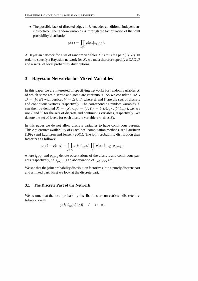
• The possible lack of directed edges inD encodes conditional independen-cies between the random variablesX through the factorization of the jointprobability distribution,
p(x) =∏
v∈V
p(xv|xpa(v)).
A Bayesian network for a set of random variablesX is thus the pair(D,P). Inorder to specify a Bayesian network forX, we must therefore specify a DAGDand a setP of local probability distributions.
3 Bayesian Networks for Mixed Variables
In this paper we are interested in specifying networks for random variablesXof which some are discrete and some are continuous. So we consider a DAGD = (V, E) with verticesV = ∆ ∪ Γ, where∆ andΓ are the sets of discreteand continuous vertices, respectively. The correspondingrandom variablesXcan then be denotedX = (Xv)v∈V = (I, Y ) = ((Iδ)δ∈∆, (Yγ)γ∈Γ), i.e. weuseI andY for the sets of discrete and continuous variables, respectively. Wedenote the set of levels for each discrete variableδ ∈ ∆ asIδ.
In this paper we do not allow discrete variables to have continuous parents.Thise.g.ensures availability of exact local computation methods, see Lauritzen(1992) and Lauritzen and Jensen (2001). The joint probability distribution thenfactorizes as follows:
p(x) = p(i, y) =∏
δ∈∆
p(iδ|ipa(δ))∏
γ∈Γ
p(yγ |ipa(γ), ypa(γ)),
whereipa(γ) andypa(γ) denote observations of the discrete and continuous par-ents respectively,i.e. ipa(γ) is an abbreviation ofipa(γ)∩∆ etc.
We see that the joint probability distribution factorizes into a purely discrete partand a mixed part. First we look at the discrete part.
3.1 The Discrete Part of the Network
We assume that the local probability distributions are unrestricted discrete dis-tributions with
p(iδ|ipa(δ)) ≥ 0 ∀ δ ∈ ∆.
16 PAPER I
A way to parameterize this is to let
θiδ |ipa(δ)= p(iδ|ipa(δ), θδ|ipa(δ)
), (1)
whereθδ|ipa(δ)= (θiδ|ipa(δ)
)iδ∈Iδ.
Then∑
iδ∈Iδθiδ |ipa(δ)
= 1 and0 ≤ θiδ |ipa(δ)≤ 1. All parameters associated
with a nodeδ is denotedθδ, i.e.θδ = (θδ|ipa(δ))ipa(δ)∈Ipa(δ)
.
Using this parameterization, the discrete part of the jointprobability distributionis given by
p(i|(θδ)δ∈∆) =∏
δ∈∆
p(iδ|ipa(δ), θδ|ipa(δ)).
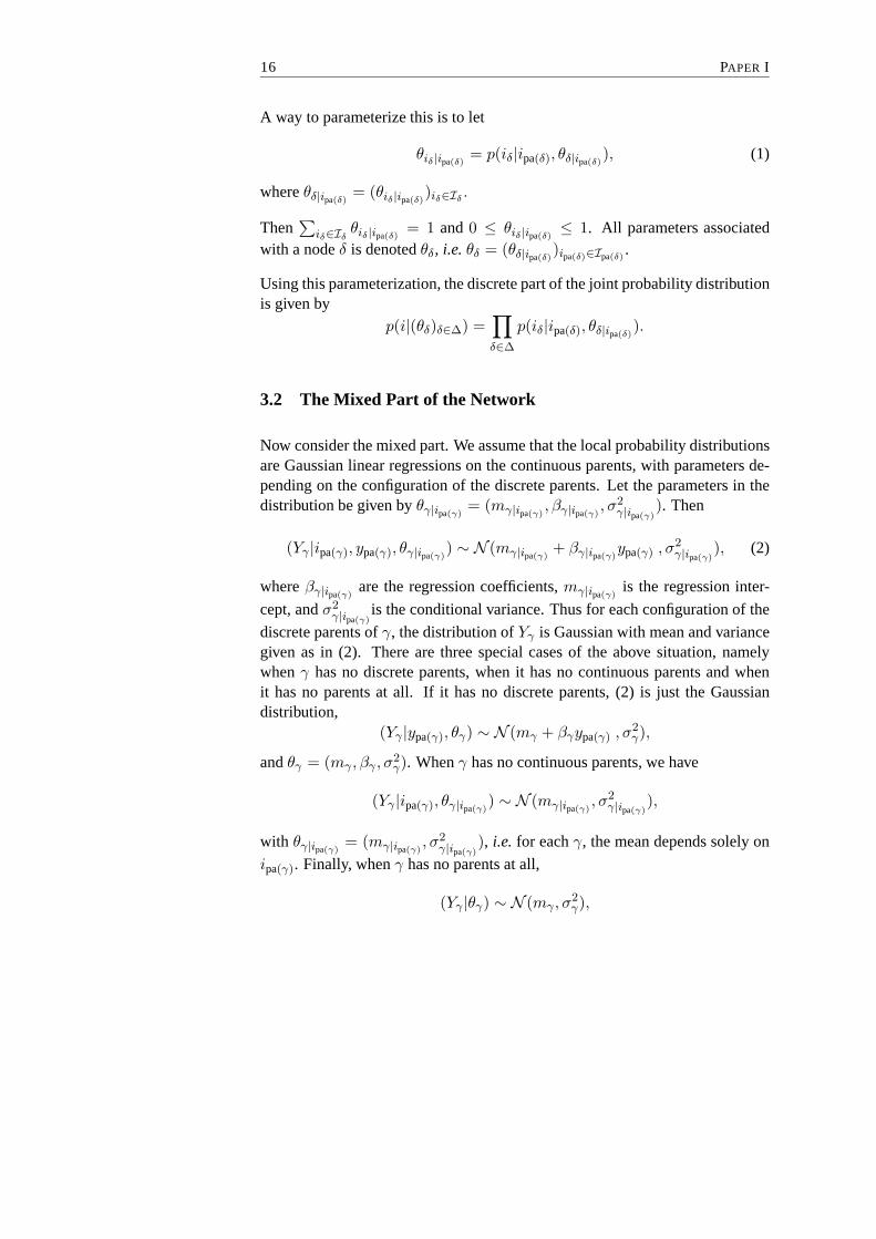
3.2 The Mixed Part of the Network
Now consider the mixed part. We assume that the local probability distributionsare Gaussian linear regressions on the continuous parents,with parameters de-pending on the configuration of the discrete parents. Let theparameters in thedistribution be given byθγ|ipa(γ)
= (mγ|ipa(γ), βγ|ipa(γ)
, σ2γ|ipa(γ)
). Then
(Yγ |ipa(γ), ypa(γ), θγ|ipa(γ)) ∼ N (mγ|ipa(γ)
+ βγ|ipa(γ)ypa(γ) , σ2
γ|ipa(γ)), (2)
whereβγ|ipa(γ)are the regression coefficients,mγ|ipa(γ)
is the regression inter-
cept, andσ2γ|ipa(γ)
is the conditional variance. Thus for each configuration of the
discrete parents ofγ, the distribution ofYγ is Gaussian with mean and variancegiven as in (2). There are three special cases of the above situation, namelywhenγ has no discrete parents, when it has no continuous parents and whenit has no parents at all. If it has no discrete parents, (2) is just the Gaussiandistribution,
(Yγ |ypa(γ), θγ) ∼ N (mγ + βγypa(γ) , σ2γ),
andθγ = (mγ , βγ , σ2γ). Whenγ has no continuous parents, we have
(Yγ |ipa(γ), θγ|ipa(γ)) ∼ N (mγ|ipa(γ)
, σ2γ|ipa(γ)
),
with θγ|ipa(γ)= (mγ|ipa(γ)
, σ2γ|ipa(γ)
), i.e. for eachγ, the mean depends solely on
ipa(γ). Finally, whenγ has no parents at all,
(Yγ |θγ) ∼ N (mγ , σ2γ),
LEARNING CONDITIONAL GAUSSIAN NETWORKS 17
with θγ = (mγ , σ2γ).
With θγ = (θγ|ipa(γ))ipa(γ)∈Ipa(γ)
, the mixed part of the joint distribution can bewritten as
p(y|i, (θγ)γ∈Γ) =∏
γ∈Γ
p(yγ |ipa(γ), ypa(γ), θγ|ipa(γ)).
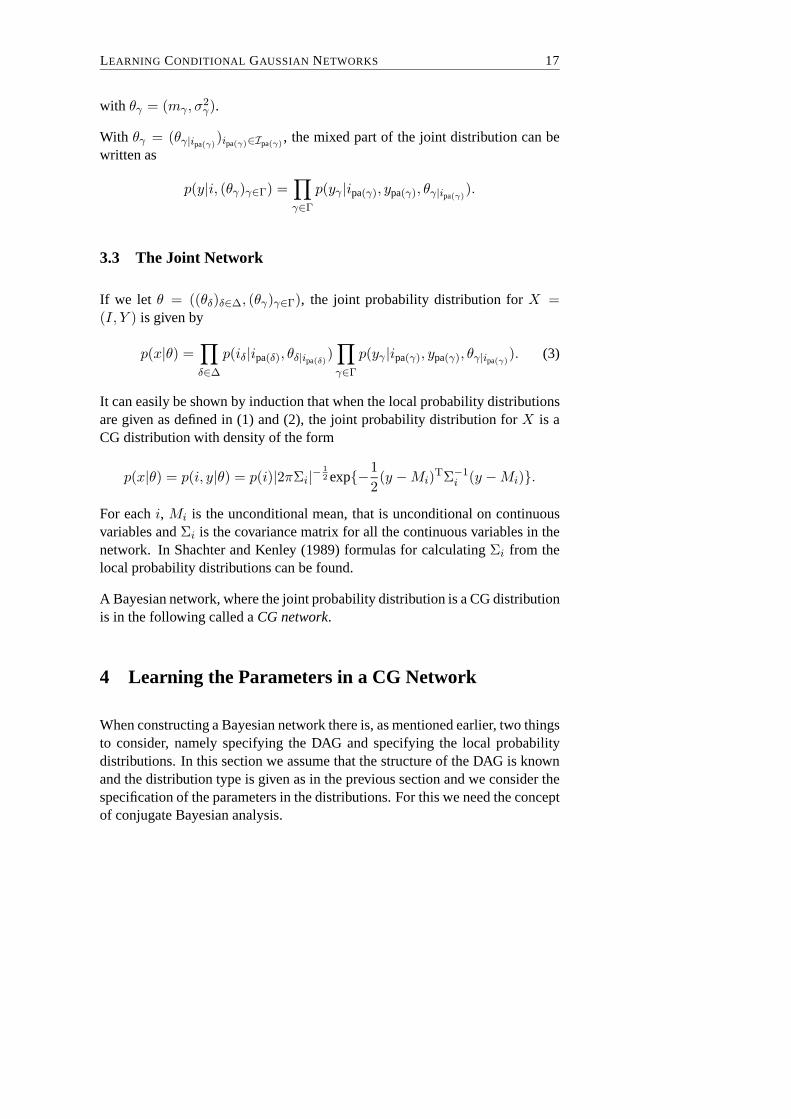
3.3 The Joint Network
If we let θ = ((θδ)δ∈∆, (θγ)γ∈Γ), the joint probability distribution forX =(I, Y ) is given by
p(x|θ) =∏
δ∈∆
p(iδ|ipa(δ), θδ|ipa(δ))∏
γ∈Γ
p(yγ |ipa(γ), ypa(γ), θγ|ipa(γ)). (3)
It can easily be shown by induction that when the local probability distributionsare given as defined in (1) and (2), the joint probability distribution for X is aCG distribution with density of the form
p(x|θ) = p(i, y|θ) = p(i)|2πΣi|− 1
2 exp{−1
2(y −Mi)
TΣ−1i (y −Mi)}.
For eachi, Mi is the unconditional mean, that is unconditional on continuousvariables andΣi is the covariance matrix for all the continuous variables inthenetwork. In Shachter and Kenley (1989) formulas for calculating Σi from thelocal probability distributions can be found.
A Bayesian network, where the joint probability distribution is a CG distributionis in the following called aCG network.
4 Learning the Parameters in a CG Network
When constructing a Bayesian network there is, as mentionedearlier, two thingsto consider, namely specifying the DAG and specifying the local probabilitydistributions. In this section we assume that the structureof the DAG is knownand the distribution type is given as in the previous sectionand we consider thespecification of the parameters in the distributions. For this we need the conceptof conjugate Bayesian analysis.

18 PAPER I
4.1 Conjugate Bayesian Analysis
There are several ways of assessing the parameters in probability distributions.An expert could specify them, or they could be estimated fromdata. In ourapproach we encode our uncertainty about the parameterθ in aprior distributionp(θ), use data to update this distribution,i.e. learn the parameter and hereby, byusing Bayes’ theorem, obtain theposteriordistributionp(θ|data), see DeGroot(1970).
Consider a situation with one random variableX. Let θ be the parameter tobe assessed,Θ the parameter space andd a random sample of sizen from theprobability distributionp(x|θ). We calld our database andxc ∈ d a case. Then,according to Bayes’ theorem,
p(θ|d) =p(d|θ)p(θ)
p(d), θ ∈ Θ, (4)
wherep(d|θ) =∏
xc∈d p(xc|θ) is the joint probability distribution ofd, alsocalled the likelihood ofθ. Furthermore the denominator is given by
p(d) =
∫
Θp(d|θ)p(θ)dθ,
and for fixedd it may be considered as a normalizing constant. Therefore (4)can be expressed as
p(θ|d) ∝ p(d|θ)p(θ),
where the proportionality constant is determined by the relation∫
Θ p(θ|d)dθ =1.
When the prior distribution belongs to a given family of distributions and theposterior distribution, after sampling from a specific distribution, belongs tothe same family of distributions, then this family is said tobe closed undersampling and called aconjugate familyof distributions. Further, if a parameteror the distribution of a parameter has a certain property which is preserved undersampling, then this property is said to be aconjugate property.
In a conjugate family of distributions it is generally straightforward to calculatethe posterior distribution.

LEARNING CONDITIONAL GAUSSIAN NETWORKS 19
4.2 Some Simplifying Properties
In the previous section we showed how to update a prior distribution for a sin-gle parameterθ. In a Bayesian network with more than one variable, we alsohave to look at the relationship between the different parameters for the dif-ferent variables in the network. In this paper we assume thatthe parametersassociated with one variable is independent of the parameters associated withthe other variables. This assumption was introduced by Spiegelhalter and Lau-ritzen (1990) and we denote itglobal parameter independence. In addition tothis, we will assume that the parameters are independent foreach configurationof the discrete parents, which we denote aslocal parameter independence. Soif the parameters have the property of global parameter independence and localparameter independence, then
p(θ) =∏
δ∈∆
∏
ipa(δ)∈Ipa(δ)
p(θδ|ipa(δ))∏
γ∈Γ
∏
ipa(γ)∈Ipa(γ)
p(θγ|ipa(γ)), (5)
and we will refer to (5) simply asparameter independence.
A consequence of parameter independence is that, for each configuration of thediscrete parents, we can update the parameters in the local distributions inde-pendently. This also means that if we havelocal conjugacy, i.e. the distributionsof θδ|ipa(δ)
andθγ|ipa(γ)belongs to a conjugate family, then because of parameter
independence, we haveglobal conjugacy, i.e. the joint distribution ofθ belongsto a conjugate family.
Further, we will assume that the databased is complete, that is, in each case itcontains at least one instance of every random variable in the network. With thiswe can show that parameter independence is a conjugate property.
Due to the factorization (3) and the assumption of complete data,
p(d|θ) =∏
c∈d
p(xc|θ)
=∏
c∈d
∏
δ∈∆
p(icδ|icpa(δ), θδ|ipa(δ)
)∏
γ∈Γ
p(ycγ |y
cpa(γ), i
cpa(γ), θγ|ipa(γ)
)
,
whereic andyc respectively denotes the discrete part and the continuous part of

20 PAPER I
a casexc. Another way of writing the above equation is
p(d|θ) =∏
δ∈∆
∏
ipa(δ)∈Ipa(δ)
∏
c:icpa(δ)=ipa(δ)
p(icδ|ipa(δ), θδ|ipa(δ))
×∏
γ∈Γ
∏
ipa(γ)∈Ipa(γ)
∏
c:icpa(γ)=ipa(γ)
p(ycγ |y
cpa(γ), ipa(γ), θγ|ipa(γ)
),(6)
where the product over cases is split up into a product over the configurations ofthe discrete parents and a product over those cases, where the configuration ofthe discrete parents is the same as the currently processed configuration. Noticehowever that some of the parent configurations might not be represented in thedatabase, in which case the product over cases with this parent configurationjust adds nothing to the overall product.
By combining (5) and (6) it is seen that
p(θ|d) =∏
δ∈∆
∏
ipa(δ)∈Ipa(δ)
p(θδ|ipa(δ)|d)∏
γ∈Γ
∏
ipa(γ)∈Ipa(γ)
p(θγ|ipa(γ)|d),
i.e. the parameters remain independent given data. We call this propertyposte-rior parameter independence. In other words, the properties of local and globalindependence are conjugate.
Notice that the posterior distribution,p(θ|d), can be found usingbatchlearningor sequentiallearning. In batch learning,p(θ|d) is found by updatingp(θ) withall cases ind at the same time,i.e. in a batch. In sequential learning,p(θ)is updated one case at a time, using the previous posterior distribution as theprior distribution for the next case to be considered. When the databased iscomplete, batch learning and sequential learning leads to the same posteriordistribution and the final result is independent of the orderin which the cases ind are processed. It is of course also possible to process some of the cases in abatch and the rest sequentially, which could be done ife.g.a new case is addedto an already processed database, see Bernardo and Smith (1994).
4.3 Learning in the Discrete Case
We now consider batch learning of the parameters in the discrete part of thenetwork. Recall that the local probability distributions are unrestricted discretedistributions defined as in (1). As pointed out in the previous section we can,
LEARNING CONDITIONAL GAUSSIAN NETWORKS 21
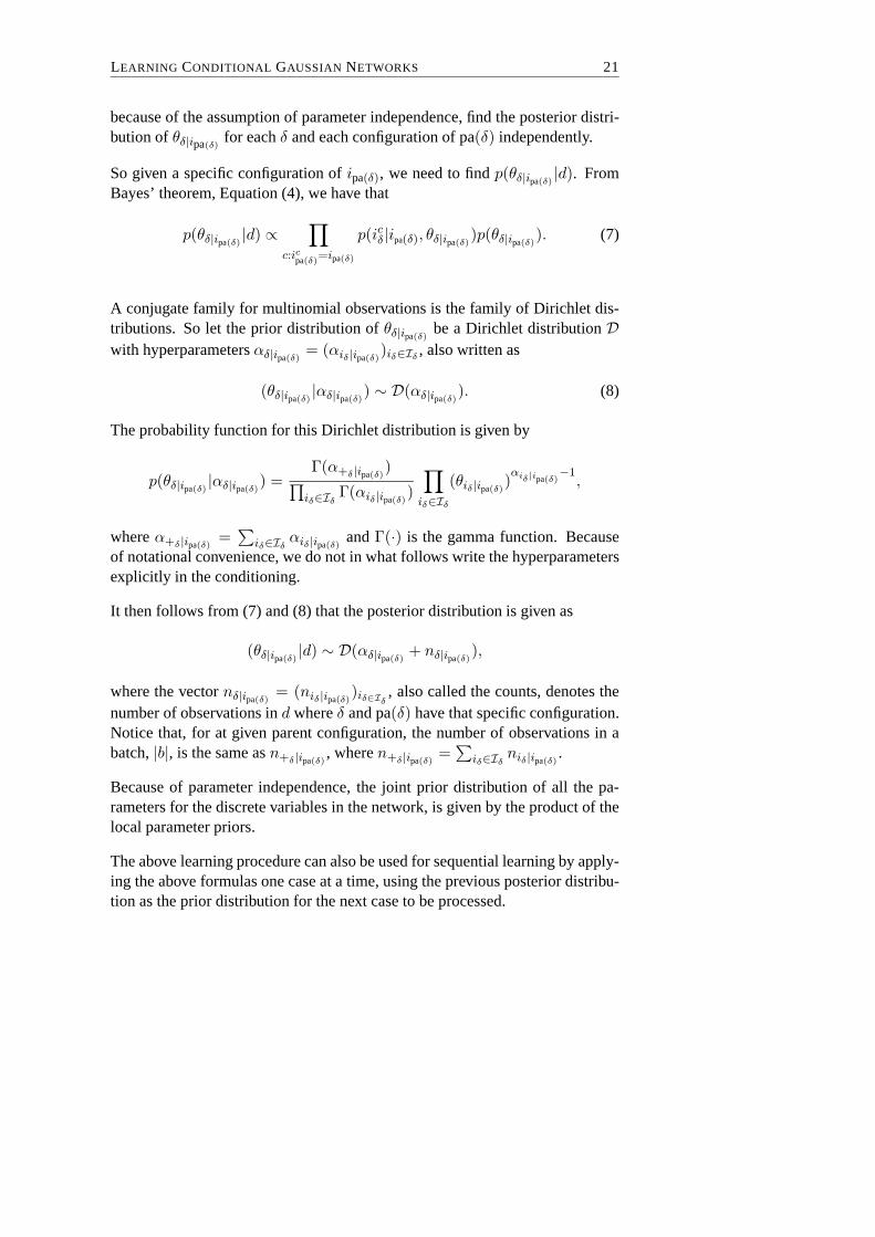
because of the assumption of parameter independence, find the posterior distri-bution ofθδ|ipa(δ) for eachδ and each configuration of pa(δ) independently.
So given a specific configuration ofipa(δ), we need to findp(θδ|ipa(δ)|d). From
Bayes’ theorem, Equation (4), we have that
p(θδ|ipa(δ)|d) ∝
∏
c:icpa(δ)=ipa(δ)
p(icδ|ipa(δ), θδ|ipa(δ))p(θδ|ipa(δ)
). (7)
A conjugate family for multinomial observations is the family of Dirichlet dis-tributions. So let the prior distribution ofθδ|ipa(δ)
be a Dirichlet distributionDwith hyperparametersαδ|ipa(δ)
= (αiδ|ipa(δ))iδ∈Iδ
, also written as
(θδ|ipa(δ)|αδ|ipa(δ)
) ∼ D(αδ|ipa(δ)). (8)
The probability function for this Dirichlet distribution is given by
p(θδ|ipa(δ)|αδ|ipa(δ)
) =Γ(α+δ|ipa(δ)
)∏
iδ∈IδΓ(αiδ|ipa(δ)
)
∏
iδ∈Iδ
(θiδ|ipa(δ))αiδ |ipa(δ)
−1,
whereα+δ |ipa(δ)=∑
iδ∈Iδαiδ|ipa(δ)
andΓ(·) is the gamma function. Becauseof notational convenience, we do not in what follows write the hyperparametersexplicitly in the conditioning.
It then follows from (7) and (8) that the posterior distribution is given as
(θδ|ipa(δ)|d) ∼ D(αδ|ipa(δ)
+ nδ|ipa(δ)),
where the vectornδ|ipa(δ)= (niδ|ipa(δ)
)iδ∈Iδ, also called the counts, denotes the
number of observations ind whereδ and pa(δ) have that specific configuration.Notice that, for at given parent configuration, the number ofobservations in abatch,|b|, is the same asn+δ|ipa(δ)
, wheren+δ|ipa(δ)=∑
iδ∈Iδniδ|ipa(δ)
.
Because of parameter independence, the joint prior distribution of all the pa-rameters for the discrete variables in the network, is givenby the product of thelocal parameter priors.
The above learning procedure can also be used for sequentiallearning by apply-ing the above formulas one case at a time, using the previous posterior distribu-tion as the prior distribution for the next case to be processed.

22 PAPER I
4.4 Learning in the Mixed Case
In the mixed case we write the local probability distributions as
(Yγ |ipa(γ), ypa(γ), θγ|ipa(γ)) ∼ N (zpa(γ)(mγ|ipa(γ)
, βγ|ipa(γ))T, σ2
γ|ipa(γ)),
wherezpa(γ) = (1, ypa(γ)). This vector has dimensionk + 1, wherek is thenumber of continuous parents toγ.
As in the discrete case we can because of parameter independence update theparameters for eachγ and each configuration of the discrete parents indepen-dently. By Bayes’ theorem,
p(θγ|ipa(γ)|d) ∝
∏
c:icpa(γ)=ipa(γ)
p(ycγ |y
cpa(γ), ipa(γ), θγ|ipa(γ)
)p(θγ|ipa(γ)).
We now join all the observationsycγ for which ic
pa(γ) = ipa(γ) in a vectorybγ , i.e.
ybγ = (yc
γ)icpa(γ)=ipa(γ)
. The same is done with the observations of the continuous
parents ofγ, i.e. ybpa(γ) = (yc
pa(γ))icpa(γ)=ipa(γ)
. As the observations ind are inde-
pendent,p(ybγ |y
bpa(γ), ipa(γ), θγ|ipa(γ)
) is the likelihood function for a multivariate
normal distribution with mean vectorzbpa(γ)(mγ|ipa(γ)
, βγ|ipa(γ))T and covariance
matrix σ2γ|ipa(γ)
I, whereI is the identity matrix andzbpa(γ) is defined through
ybpa(γ).
The posterior distribution ofθγ|ipa(γ)can now be written as
p(θγ|ipa(γ)|d) ∝ p(yb
γ |ybpa(γ), ipa(γ), θγ|ipa(γ)
)p(θγ|ipa(γ)).
A standard conjugate family for these observations is the family of Gaussian-inverse gamma distributions. Let the prior joint distribution of (mγ|ipa(γ)
, βγ|ipa(γ))
andσ2γ|ipa(γ)
be as follows.
(mγ|ipa(γ), βγ|ipa(γ)
|σ2γ|ipa(γ)
) ∼ Nk+1(µγ|ipa(γ), σ2
γ|ipa(γ)τ−1γ|ipa(γ)
)
(σ2γ|ipa(γ)
) ∼ IΓ
(
ργ|ipa(γ)
2,φγ|ipa(γ)
2
)
.

LEARNING CONDITIONAL GAUSSIAN NETWORKS 23
The posterior distribution is then
(mγ|ipa(γ), βγ|ipa(γ)
|σ2γ|ipa(γ)
, d) ∼ Nk+1(µ′γ|ipa(γ)
, σ2γ|ipa(γ)
(τ−1γ|ipa(γ)
)′)
(σ2γ|ipa(γ)
|d) ∼ IΓ
(
ρ′γ|ipa(γ)
2,φ′
γ|ipa(γ)
2
)
,
where
τ ′γ|ipa(γ)
= τγ|ipa(γ)+ (zb
pa(γ))Tzb
pa(γ)
µ′γ|ipa(γ)
= (τ ′γ|ipa(γ)
)−1(τγ|ipa(γ)µγ|ipa(γ)
+ (zbpa(γ))
Tybγ)
ρ′γ|ipa(γ)= ργ|ipa(γ)
+ |b|
φ′γ|ipa(γ)
= φγ|ipa(γ)+ (yb
γ − zbpa(γ)µ
′γ|ipa(γ)
)Tybγ
+(µγ|ipa(γ)− µ′
γ|ipa(γ))Tτγ|ipa(γ)
µγ|ipa(γ),
where|b| denotes the number of observations inb.
As for the discrete variables, we can with these formulas also use the sequentialapproach and update the parameters one case at a time.
Further, because of parameter independence, the joint prior distribution is givenas the product of the local prior distributions for all parameters in the network.
5 Learning the Structure of a CG Network
In this section we consider how to learn the structure of a CG network.
5.1 The Network Score
There are basically two ways of determining which DAG shouldrepresent theconditional independencies between a set of random variables. First, if the re-lations between the variables are well understood by an expert, then he couldspecify the DAG, using a causal interpretation of the arrows. Second, we couldlearn the DAG from data. That is, we could find out how well a DAGD rep-resents the conditional independencies, by measuring how probableD is, giventhat we have observed datad. Different approaches use different measures. An

24 PAPER I
often used measure is the posterior probability of the DAG,p(D|d), which fromBayes’ theorem is given by
p(D|d) ∝ p(d|D)p(D),
wherep(d|D) is the likelihood ofD andp(D) is the prior probability. As thenormalizing constant does not depend upon structure, another measure, whichgives the relative probability, is
p(D, d) = p(d|D)p(D).
We refer to the above measures asnetwork scores. So learning the DAG fromdata, we can in principle first calculate the network scores for all possible DAGsand then select the DAG with the highest network score. If many DAGs arepossible, it is computationally infeasible to calculate the network score for allthese DAGs. In this situation it is necessary to use some kindof search strategyto find the DAG with the highest score, seee.g.Cooper and Herskovits (1992).
In some cases it can be more accurate to average over the possible DAGs forprediction, instead of just selecting a single DAG. So ifx is the quantity we areinterested in, we can use the weighted average,
p(x|d) =∑
D∈DAG
p(x|d, D)p(D|d),
whereDAG is the set of all DAGs andp(D|d) is the weight.
Again, if many DAGs are possible, this sum is to heavy to compute, so instead,by using a search strategy, we can find a few DAGs with high score and averageover these.
5.2 The Network Score for a CG Network
In order to calculate the network score for a specific DAGD, we need to knowthe prior probability and the likelihood of the DAG. For simplicity, we could forexample choose to let all DAGs be equally likely, then
p(D|d) ∝ p(d|D).

LEARNING CONDITIONAL GAUSSIAN NETWORKS 25
In a CG network, the likelihood of the DAGD is given by
p(d|D) =
∫
θ∈Θp(d|θ, D)p(θ|D)dθ
=∏
δ∈∆
∏
ipa(δ)∈Ipa(δ)
∫
∏
c:icpa(δ)=ipa(δ)
p(icδ|ipa(δ), θδ|ipa(δ), D)p(θδ|ipa(δ)
|D)dθδ|ipa(δ)
×∏
γ∈Γ
∏
ipa(γ)∈Ipa(γ)
∫
∏
c:icpa(γ)=ipa(γ)
p(ycγ |y
cpa(γ), ipa(γ), θγ|ipa(γ)
, D)p(θγ|ipa(γ)|D)dθγ|ipa(γ)
.
Again we see that we can consider the problem for the discretepart and themixed part of the network separately.
The discrete part is from the formulas in Section 4.3 found tobe
∏
δ∈∆
∏
ipa(δ)∈Ipa(δ)
Γ(α+δ|ipa(δ))
Γ(α+δ|ipa(δ)+ n+δ|ipa(δ)
)
∏
iδ∈Iδ
Γ(αiδ|ipa(δ)+ niδ |ipa(δ)
)
Γ(αiδ|ipa(δ))
.
In the mixed part of the network, the local marginal likelihoods are non-centraltdistributions withργ|ipa(γ)
degrees of freedom, location vectorzbpa(γ)µγ|ipa(γ)
and
scale parametersγ|ipa(γ)=
φγ|ipa(γ)
ργ|ipa(γ)
(I + (zbpa(γ))τ
−1γ|ipa(γ)
(zbpa(γ))
T). The indexb
is defined as in Section 4.4.
So the mixed part is given by
∏
γ∈Γ
∏
ipa(γ)∈Ipa(γ)
Γ((ργ|ipa(γ)+ |b|)/2)
Γ(ργ|ipa(γ)/2)[det(ργ|ipa(γ)
sγ|ipa(γ)π)]
12
×
[
1 +1
ργ|ipa(γ)
(ybγ − zb
pa(γ)µγ|ipa(γ))s−1
γ|ipa(γ)(yb
γ − zbpa(γ)µγ|ipa(γ)
)T
]
−(ργ|ipa(γ)+|b|)
2
.
The network score for a CG network is thus the product of the prior probabilityfor the DAGD, the term for the discrete part and the term for the mixed part.Notice that the network score has the property that it factorizes into a productover terms involving only one node and its parents. This property is calleddecomposability.
To evaluate which DAG or possible several DAGs that represent the conditionalindependencies in a Bayesian network well, we want to find theDAG or DAGs

26 PAPER I
with the highest network scores. To calculate these scores,we must specify thelocal probability distributions and the local prior distributions for the parametersfor each network under evaluation. In the next section, a method for doing thisis developed.
6 The Master Prior Procedure
The papers Heckerman et al. (1995) and Geiger and Heckerman (1994) developsa method for finding the prior distributions for the parameters in respectivelythe purely discrete case and the purely continuous case. Thework is basedon principles of likelihood equivalence, parameter modularity, and parameterindependence. It leads to a method where the parameter priors for all possiblenetworks are deduced from one joint prior distribution, in the following calleda master priordistribution.
In this paper we will build on this idea, which can be used on networks withmixed variables. We will therefore in the following describe their method forthe pure cases.
6.1 The Master Prior in the Discrete Case
In the purely discrete case, or the discrete part of a mixed network, the followingis a well known classical result.
Let A be a subset of∆ and letB = ∆ \A. Let the discrete variablesi have thejoint distribution
p(i|Ψ) = Ψi.
Notice here, that the setΨ = (Ψi)i∈I contains the parameters for the jointdistribution, contrary toθ in Section 3, which contains the parameters for theconditional local distributions.
In the following we use the notationziA =∑
j:jA=iAzj , wherez is any param-
eter. Then the marginal distribution ofiA is given by
p(iA|Ψ) = ΨiA ,
and the conditional distribution ofiB giveniA is
p(iB|iA, Ψ) =Ψi
ΨiA
= ΨiB |iA .

LEARNING CONDITIONAL GAUSSIAN NETWORKS 27
Further if the joint prior distribution for the parametersΨ is Dirichlet, that is
(Ψ) ∼ D(α),
whereα = (αi)i∈I , then the marginal distribution ofΨA is Dirichlet, i.e.
(ΨA) ∼ D(αA),
with αA = (αiA)iA∈IA. The conditional distribution ofΨB|iA is
(ΨB|iA) ∼ D(αB|iA),
with αB|iA = (αiB |iA)iB∈IBandαiB |iA = αi. Furthermore the parameters are
independent, that is
p(Ψ) =∏
iA∈IA
p(ΨB|iA)p(ΨA). (9)
From the above result we see, that for each possible parent/child relationship, wecan find the marginal parameter priorp(Ψδ∪pa(δ)). Further, from this marginaldistribution we can, for each configuration of the parents, find the conditionallocal prior distributionp(Ψδ|ipa(δ)
). Notice thatΨδ|ipa(δ)= θδ|ipa(δ)
, whereθδ|ipa(δ)
was specified for the conditional distributions in Section (3.1). Further, becauseof parameter independence, given by (9), we can find the jointparameter priorfor any network as the product of the local priors involved.
To use this method, we must therefore specify the joint Dirichlet distribution,i.e. the master Dirichlet prior. This was first done in Heckerman et al. (1995) andhere we follow their method. We start by specifying a prior Bayesian network(D,P). From this we calculate the joint distributionp(i|Ψ) = Ψi. To specify amaster Dirichlet distribution, we must specify the parametersα = (αiδ)i∈I andfor this we use the following relation for the Dirichlet distribution,
p(i) = E(Ψi) =αi
n,
with n =∑
i∈I αi. Now we let the probabilities in the prior network be anestimate ofE(Ψi), so we only need to determinen in order to calculate theparametersαi. We determinen by using the notion of an imaginary database.We imagine that we have a database of cases, from which we fromtotal igno-rance have updated the distribution ofΨ. The sample size of this imaginarydatabase is thusn. Therefore we refer to the estimate ofn as theimaginarysample sizeand it expresses how much confidence we have in the dependencystructure expressed in the prior network.

28 PAPER I
6.2 The Master Prior in the Gaussian Case
For the Gaussian case, the following result is used, seee.g.Dawid and Lauritzen(1993). LetA be a subset ofΓ and letB = Γ \A. If
(y|m, Σ) ∼ N (m, Σ),
then(yA|m, Σ) ∼ N (mA, ΣAA)
and(yB|yA, mB|A, βB|A, ΣB|A) ∼ N (mB|A + βB|AyA, ΣB|A),
where
Σ =
(
ΣAA ΣAB
ΣBA ΣBB
)
, ΣB|A = ΣBB − ΣBAΣ−1AAΣAB ,
mB|A = mB − βB|AmA and βB|A = ΣBAΣ−1AA.
Further, if
(m|Σ) ∼ N (µ,1
νΣ) and (Σ) ∼ IW (ρ, Φ),
where the scale matrixΦ is partitioned asΣ, then
• (mA|ΣAA) ∼ N (µA, 1ν ΣAA)
• (ΣAA) ∼ IW (ρ, ΦAA)
• (ΣB|A) ∼ IW (ρ + |A|, ΦB|A)
• (mB|A, βB|A|ΣB|A) ∼ N (µB|A, ΣB|A ⊗ τ−1B|A)
• mA, ΣAA ⊥⊥ mB|A, βB|AΣB|A
whereµB|A = (µB − ΦBAΦ−1
AAµA, ΦBAΦ−1AA)
and
τ−1B|A
=
1ν + µT
AΦ−1AAµA −µT
AΦ−1AA
−Φ−1AAµA Φ−1
AA
,
and⊗ denotes the Kronecker product. Notice that the dimension ofµB|A isgiven as(|B|, |B| × |A|).
As in the discrete case, this result shows us how to deduce thelocal proba-bility distributions and the local prior distributions from the joint distributions.

LEARNING CONDITIONAL GAUSSIAN NETWORKS 29
Further, because of parameter independence, the joint parameter prior for anyGaussian network can be specified as the product of the local priors. Noticethat the parameters found here for a node given its parents, coincides with theparameters specified in Section 3.2.
Before we show how to construct the master prior, we need the following result.The Gaussian-inverse Wishart prior is conjugate to observations from a Gaus-sian distribution (DeGroot 1970). So let the probability distribution and the priordistribution be given as above. Then, given the databased = {y1, . . . , yn}, theposterior distributions are
(m|Σ, d) ∼ N (µ′,1
ν ′Σ) and (Σ|d) ∼ IW (ρ′, Φ′),
where
ν ′ = ν + n,
µ′ =νµ + ny
ν + n, (10)
ρ′ = ρ + n,
Φ′ = Φ + ssd +νn
ν + n(µ− y)(µ− y)T,
with
y =1
n
n∑
i=1
yi and ssd =n∑
i=1
(yi − y)(yi − y)T.
From these updating formulas we see thatν ′ andρ′ are updated with the numberof cases in the database. Furtherµ′ is a weighted average of the prior mean andthe sample mean, each weighted by their sample sizes. Finally Φ is updated withthe ssd, which expresses how much each observation differs from thesamplemean, and an expression for how much the prior mean differs from the samplemean.
To specify the master prior, we need to specify the four parametersν, µ, ρ andΦ. As for the discrete variables we start by specifying a priorBayesian network,(D,P). From this, a prior joint probability distributionp(y|m, Σ) = N (m, Σ)can be deduced. Now imagine that the meanm and the varianceΣ were cal-culated from an imaginary database, so that they actually are the sample meanand the sample variance. Further, assume that before this imaginary databasewas observed, we were totally ignorant about the parameters. The formulas in(10) can now be used to “update” the parameters on the basis ofthe imaginary

30 PAPER I
database. As we have not seen any cases before,ν andρ are estimated by thesize of the imaginary database. Further
µ = m and Φ = ssd = (ν − 1)Σ.
In Geiger and Heckerman (1994),µ andΦ are found in a slightly different way.They use the fact that the marginal likelihoodp(y) is a multivariate non-centralt distribution with ρ degrees of freedom, location vectorµ and scale matrixS = ν+1
νρ Φ. Now the mean and covariance matrix in thet distribution is givenby
E(y) = µ and Cov(y) =ρ
ρ− 2S.
They then let the mean and covariance matrix from the prior network estimatethe mean and covariance matrix in thet distribution, which implies that
µ = m and Φ =ν(ρ− 2)
ν + 1Σ.
Experimental results have not shown noticeable differences between the twoapproaches.
6.3 Properties of the Master Prior Procedure
The method for finding prior parameter distributions described in the previoussection has some properties, which we will describe here. Inthis section we useΨ as a parameter defined for a joint distribution,i.e.Ψ can be the parameter forthe discrete variables or in the continuous case,Ψ = (m, Σ).
Clearly a consequence of using the above method is that the parameters areindependent. Further it can be seen, that if a nodev has the same parents in twoDAGsD andD∗, then
p(Ψv|pa(v)|D) = p(Ψv|pa(v)|D∗).
This property is referred to asparameter modularity. Now both the discrete andthe Gaussian distribution has the property that if the jointprobability distribu-tion p(x) can be factorized according to a DAGD, then it can also be factorizedaccording to all other DAGs, which represents the same set ofconditional inde-pendencies asD. A set of DAGs,De, which represents the same independenceconstraints is referred to asindependence equivalentDAGs. So letD andD∗
be independence equivalent DAGs, then
p(x|Ψ, D) = p(x|Ψ, D∗).
LEARNING CONDITIONAL GAUSSIAN NETWORKS 31
This means, that from observations alone we can not distinguish between dif-ferent DAGs in an equivalence class. In the papers Heckermanet al. (1995) andGeiger and Heckerman (1994) it is for respectively the discrete and the Gaussiancase shown, that when using the master prior procedure for the construction ofparameter priors, the marginal likelihood for data is also the same for indepen-dence equivalent networks,i.e.
p(d|D) = p(d|D∗).
This equivalence is referred to aslikelihood equivalence. Note that likelihoodequivalence imply that ifD andD∗ are independence equivalent networks, thenthey have the same joint prior for the parameters,i.e.
p(Ψ|D) = p(Ψ|D∗).
7 Local Masters for Mixed Networks
In this section we will show how to specify prior distributions for the parametersin a CG network. In the mixed case, the marginal of a CG distribution is notalways a CG distribution. In fact it is only a CG distributionif we marginalizeover continuous variables or if we marginalize over a setB of discrete variable,where(B ⊥⊥ Γ) | (∆ \ B), see Frydenberg (1990). Consider the followingexample. We have a network of two variables,i andy, and the joint distributionis given by
p(i, y) = p(i)N (mi, σ2i ).
Then the marginal distribution ofy is given as a mixture of normal distributions
p(y) =∑
i∈I
p(i)N (mi, σ2i ),
so there is no simple way of using this directly for finding thelocal priors.
7.1 The Suggested Solution
The suggested solution is very similar to the solution for the pure cases. We startby specifying a prior Bayesian network(D,P) and calculate the joint probabil-ity distribution
p(i, y|H) = p(i|Ψ)N (mi, Σi),

32 PAPER I
with H = (Ψ, (mi)i∈I , (Σi)i∈I). So from the conditional parameters in thelocal distributions in the prior network, we calculate the parameters for the jointdistribution. Then we translate this prior network into an imaginary database,with imaginary sample sizen. From the probabilities in the discrete part ofthe network, we can, as in the pure discrete case, calculateαi for all configu-rations ofi. Now αi represents how many times we have observedI = i inthe imaginary database. We can assume that each time we have observed thediscrete variablesI, we have observed the continuous variablesY and thereforesetνi = ρi = αi. Now for each configuration ofi, we letmi be the samplemean in the imaginary database, andΣi the sample variance. Further, as for thepure Gaussian case, we usemi = µi andΦi = (νi − 1)Σi. However, forΦi tobe positive,νi has to larger than1, for all configurationsi and this has an impacton how small we can choosen to be, asn =
∑
i νi. If the number of discretevariables is large, and/or the number of configurations of the discrete variablesis large, then we might have to letn be larger than the value, that really reflectsour confidence in the prior network. For these situations it might therefore bebetter toe.g. let Φi = νiΣi as we then can choose the value ofn any way wewant. Or, we can just chooseνi andρi independently ofn.
All the parameters needed to define the joint prior distributions for the parame-ters are now specified, so
p(Ψ) = D(α),
p(Mi|Σi) = N (µi,1
νiΣi),
p(Σi) = IW (ρi, Φi).
But we can not use these distributions to derive priors for other networks, soinstead we use the imaginary database to derive local masterdistributions.
Let, for each familyA = v ∪ pa(v), the marginal CG distribution ofXa givenHA be given by
(XA|HA) ∼ CG(ΨiA∩∆ , mA∩Γ|iA∩∆, ΣA∩Γ|iA∩∆
).
Then we suggest that the marginal prior distributions, alsocalled thelocal mas-ters, are found in the following way:

LEARNING CONDITIONAL GAUSSIAN NETWORKS 33
Let, for any variablez, ziA∩∆ =∑
j:jA∩∆=iA∩∆zj. Then
(ΨA∩∆) ∼ D(αA∩∆),
(ΣA∩Γ|iA∩∆) ∼ IW (ρiA∩∆ , (ΦA∩Γ|iA∩∆
),
(mA∩Γ|iA∩∆|ΣA∩Γ|iA∩∆
) ∼ N (µA∩Γ|iA∩∆,
1
νiA∩∆
ΣA∩Γ|iA∩∆),
where
µiA∩∆=
(∑
j:jA∩∆=iA∩∆µjνj)
νA∩∆,
and
ΦiA∩∆ = ΦiA∩∆ +∑
j:jA∩∆=iA∩∆
νj(µj − µiA∩∆)(µj − µiA∩∆
)T.
The equations in the above result are well known from the analysis of variancetheory, seee.g.Seber (1984). The marginal mean is found as a weighted averageof the mean in every group, where a group here is given as a configurationof the discrete parents we marginalize over. The weights arethe number ofobservations in each group. The marginalssd is given as the within groupvariation plus the between group variation. Notice that with this method, it ispossible to specify mixed networks, where the mean in the mixed part of thenetwork depends on the discrete parents, but the variance does not.
From the local masters we can now, by conditioning as in the pure cases, derivethe local priors needed to specify the prior parameter distribution for a CG net-work. So the only difference between the master procedure and the local masterprocedure is in the way the marginal distributions are found.
7.2 Properties of the Local Master Procedure
The local master procedure coincides with the master procedure in the purecases. Further, the properties of the local master procedure in the mixed case,are the same as of the master prior procedure in the pure cases.
Parameter independence and parameter modularity follows immediately fromthe definition of the procedure. To show likelihood equivalence, we need thefollowing result from Chickering (1995). LetD andD∗ be two DAGs and letRD,D∗ be the set of edges by whichD andD∗ differ in directionality. Then,D andD∗ are independence equivalent if and only if there exists a sequence of|RD,D∗ | distinct arc reversals applied toD with the following properties:
34 PAPER I
• After each reversal, the resulting network structure is a DAG, i.e. it con-tains no directed cycles and it is independence equivalent to D∗.
• After all reversals, the resulting DAG is identical toD∗.
• If w → v is the next arc to be reversed in the current DAG, thenw andvhave the same parents in both DAGs, with the exception thatw is also aparent ofv in D.
Note that as we only reverse|RD,D∗ | distinct arcs, we only reverse arcs inRD,D∗ . For mixed networks this means that we only reverse arcs between dis-crete variables or between continuous variables, as the only arcs that can differin directionality are these. So we can use the above result for mixed networks.
From the above we see that we can show likelihood equivalenceby showingthatp(d|D) = p(d|D∗) for two independence equivalent DAGsD andD∗ thatdiffer only by the direction of a single arc. Asp(x|H, D) = p(x|H, D∗) inCG networks, we can show likelihood equivalence by showing thatp(H|D) =p(H|D∗).
In the following letv → w in D andw → v in D∗. Further let∇ be the setof common discrete and continuous parents forv andw. Of course, ifv andw are discrete variables, then∇ only contains discrete variables. The relationbetweenp(H|D) andp(H|D∗) is given by:
p(H|D)
p(H|D∗)=
p(Hv|w∪∇, D)p(Hw|∇, D)
p(Hw|v∪∇, D∗)p(Hv|∇, D∗)
=p(Hv∪w|∇, D)
p(Hv∪w|∇, D∗). (11)
When using the local master procedure, the terms in (11) are equal. This isevident, as we find the conditional priors from distributions over familiesA, inthis caseA = v ∪ w ∪ ∇, which is the same for both networks. Thereforelikelihood equivalence follows.
8 Model Search
In the search for Bayesian networks with high network score,we can, in theory,calculate the network score for all possible DAGs and then choose the DAG orDAGs with the highest score.

LEARNING CONDITIONAL GAUSSIAN NETWORKS 35
In Robinson (1977), a recursive formula for the number of possible DAGs thatcontainsn nodes, is found to be
f(n) =n∑
i=1
(−1)i+1
(
ni
)
2i(n−i)f(n− i),
where
(
ni
)
are the binomial coefficient. As we in mixed networks do not
allow discrete nodes to have continuous parents, the numberof possible mixedDAGs is given by
f(|∆|, |Γ)|) = f(|∆|)× f(|Γ|)× 2|∆|×|Γ|,
wheref(|∆|) andf(|Γ|) are the numbers of DAGs for respectively the discreteand the continuous nodes, and2|∆|×|Γ| denotes the number of different combi-nations of arrows from discrete to continuous nodes. If the number of randomvariables in the network is large, it is computationally infeasible to calculatethe network score for all the possible DAGs. Therefore different methods forsearching for DAGs with high network score have been tried, seee.g.Cooperand Herskovits (1992). In Section 8.3 we will describe one ofthese methods,namely greedy search with random restarts. This method, like many others,make use of Bayes factors as a way of comparing the network scores for twodifferent DAGs. In the next section we will therefore consider Bayes factors formixed networks.
8.1 Bayes Factors
A way to compare the network score for two different networks, D andD∗, isto calculate theposterior odds, given by
p(D|d)
p(D∗|d)=
p(D, d)
p(D∗, d)=
p(D)
p(D∗)×
p(d|D)
p(d|D∗),
wherep(D)/p(D∗) is theprior oddsandp(d|D)/p(d|D∗) is theBayes factor.
The posterior odds is for numerical reasons often calculated using the logarithm,
log
(
p(D|d)
p(D∗|d)
)
= log(p(D|d))− log(p(D∗|d)).
For two models that differ only by a single arrow, the Bayes factor is, becauseof decomposability, especially simple. In this section, wewill specify the Bayes

36 PAPER I
factor in the case where two DAGs differ by the direction of a single arrow andin the case where two DAGs differ by the presence of a single arrow.
First we look at the former case. As discrete nodes can not have continuousparents, we only look at reversing an arrow between two discrete variables ortwo continuous variables. In the following letv ← w in D andv → w in D∗.Further let∇w be the parents ofw in D and∇v the parents ofv in D∗. As DandD∗ only differ by the direction of the arrow betweenv andw, the parentsof w in D∗ are∇w andv and the parents ofv in D are∇v andw. Noticethat if v andw are discrete nodes, then the nodes in∇v and∇w can only bediscrete, whereas ifv andw are continuous nodes, they can be both discrete andcontinuous.
To simplify, we let the database consist of just one case, sod = {x}. As thelikelihood terms are decomposable, the Bayes factor is given by
p(x|D)
p(x|D∗)=
p(v|∇v, w, D)p(w|∇w, D)
p(w|∇w, v, D∗)p(v|∇v, D∗)
=
∫
p(xv|xw∪∇v , Hv|w∪∇v, D)p(Hv|w∪∇v
|D)dHv|w∪∇v∫
p(xw|xv∪∇w , Hw|v∪∇w, D∗)p(Hw|v∪∇w
|D∗)dHw|v∪∇w
×
∫
p(xw|x∇w , Hw|∇w, D)p(Hw|∇w
|D)dHw|∇w∫
p(xv|x∇v , Hv|∇v, D∗)p(Hv|∇v
|D∗)dHv|∇v
.
So to calculate the Bayes factor betweenD andD∗, we only need to considerthe terms involving the conditional distributions ofv and ofw.
Notice that if∇v = ∇w, thenD andD∗ are independence equivalent networksand the Bayes factor is equal to one.
Now let D and D∗ be two different networks, that differ by a single arrowbetween the nodesv andw, with v ← w in D andv 8 w in D∗. Herev andw can be either both discrete variables, both continuous orv continuous andwdiscrete. Again, let∇v be the set of variables that are parents ofv in D∗, so inD the parents ofv are∇v andw. As the likelihood terms are decomposable, theBayes factor is given by
p(x|D)
p(x|D∗)=
p(xv|xw∪∇v , D)
p(xv|x∇v , D∗)
=
∫
p(xv|xw∪∇v , Hv|w∪∇v, D)p(Hv|w∪∇v
|D)dHv|w∪∇v∫
p(xv|x∇D, Hv|∇v
, D∗)p(Hv|∇v|D∗)dHv|∇v
.
LEARNING CONDITIONAL GAUSSIAN NETWORKS 37
8.2 Equivalent Bayes Factors
To compare network scores for all networks which differ by only one arrow,is computationally inefficient. When using the local masterprocedure, we canreduce the number of comparisons needed.
Our goal is to identify classes of DAGs for which the corresponding Bayesfactors for testing an arrow between the same two variables in the network, arethe same. So letD1 andD∗
1 be two different networks that differ by a singlearrow between the nodesv andw, with v ← w in D1 andv 8 w in D∗
1. Further,let∇v1 be the set of variables that are parents ofv in bothD1 andD∗
1, i.e. in D1
the parents ofv are∇v1 andw and inD∗1 just∇D1 .
Further letD2 andD∗2 be another two networks different fromD1 andD∗
1 thatdiffer by an arrow betweenv andw and let∇v2 be the set of variables that areparents ofv in bothD2 andD∗
2. There are two situations to consider, namelywhenv ← w in D2 and whenv → w in D2.
Consider first the former situation. The Bayes factor for testing D1 againstD∗1
was in the previous section found to be
p(x|D1)
p(x|D∗1)
=
∫
p(xv|xw∪∇v1, Hv|w∪∇v1
, D1)p(Hv|w∪∇v1|D1)dHv|w∪∇v1
∫
p(xv|x∇v1, Hv|∇v1
, D∗1)p(Hv|∇v1
|D∗1)dHv|∇v1
. (12)
Likewise the Bayes factor for testingD2 againstD∗2 is
p(x|D2)
p(x|D∗2)
=
∫
p(xv|xw∪∇v2, Hv|w∪∇v2
, D2)p(Hv|w∪∇v2|D2)dHv|w∪∇v2
∫
p(xv|x∇v2, Hv|∇v2
, D∗2)p(Hv|∇v2
|D∗2)dHv|∇v2
.
As the local master procedure has the property of parameter modularity, then if∇v1 = ∇v2 it follows that
p(Hv|w∪∇v1|D1) = p(Hv|w∪∇v2
|D2),
and
p(xv|xw∪∇v1, Hv|w∪∇v1
, D1) = p(xv|xw∪∇v2, Hv|w∪∇v2
, D2).
So the Bayes factor for testing the arrow fromv to w is equivalent to testingthis arrow in any other network, wherev has the same parents as inD1, i.e. if∇v1 = ∇v2 . This is illustrated in Figure 1.

38 PAPER I
∇v
v w
∇v
v w
Figure 1: Equivalence due to parameter modularity.
∇v
v w
∇v
v w
Figure 2: Equivalence due to property of local master procedure.
Consider now the situation wherev → w in D2. Let∇w2 be the set of variables,that are parents ofw in bothD2 andD∗
2. The Bayes factor is given as
p(x|D2)
p(x|D∗2)
=p(xw|xv∪∇w2
, D2)
p(xw|x∇w2, D∗
2)
=
∫
p(xw|xv∪∇w2, Hw|v∪∇w2
, D2)p(Hw|v∪∇w2|D2)dHw|v∪∇w2
∫
p(xw|x∇w2, Hw|∇w2
, D∗2)p(Hw|∇w2
|D∗2)dHw|∇w2
.
Again we see that because of parameter modularity, this Bayes factor is the sameas the Bayes factor given in (12), if∇v1 = ∇w2 , i.e. if w in D2 has the sameparents asv does inD1, with the exception thatv is a parent ofw in D2. For anillustration, see Figure 2.
To show that these situations are the only ones where the Bayes factors alwaysare the same, it is easy to find an example where∇v1 6= ∇v2 and the Bayesfactors are not same.
The above result is summarized in the following theorem.
Theorem 8.1The Bayes factor for testing the arrowv ← w in a DAGD1 is equivalent to theBayes factor for testing the same arrow in any other networkD2 if and only ifthe following two criteria are met:
(1) v ← w andv in D2 has the same parents as inD1.

LEARNING CONDITIONAL GAUSSIAN NETWORKS 39
(2) v → w and w in D2 has the same parents asv does inD1, with theexception thatv is a parent ofw in D2.
Although using the two criteria reduces the number of comparisons, there willstill, for large networks, be too many comparisons needed for finding the mostlikely DAG. Therefore it is still necessary to use some kind of search strategy.
8.3 Greedy search with random restarts
As mentioned earlier, many search strategies use Bayes factors as a way to com-pare the network score for two different networks. In the following we willdescribe one such strategy calledgreedy search.
Greedy search is initialized by choosing a networkD from which to start thesearch. Let∆e be the posterior odds between two networks that differ by anarrow. Calculate then∆e for all DAGs D∗ that differ fromD by a single ar-row e, either added, removed or reversed. Make the changee for which ∆eis a minimum, that is wherep(D∗|d) is a maximum and continue the searchfrom this new network. The search is terminated when there isno e with ∆esmaller than1. As shown in the previous section, the posterior odds is becauseof decomposability especially simple, asD andD∗ only differ by one arrow.Further, it is possible to reduce the time complexity by using the equivalencecriteria developed in Section 8.2.
As this search is local in the sense that it only evaluates local changes to thenetwork, there is a chance that the found maximum is only a local maximum. Away to overcome this problem is to randomly perturb the structure of the startnetworkD and restart the greedy search from this new network. This canberepeated a manageable number of times and between the networks found by thesearch strategy, the network with the highest score is chosen.
8.4 Priors on DAGs
In this section we will consider how to assign prior probabilities to the possibleDAGs in a given problem. As shown in various papers, there aredifferent waysof doing this. The Bayesian way would be to assess the prior belief in eachDAG, but as the number of different DAGs grow, this is not manageable. Insteadautomated methods is being used.

40 PAPER I
D1
v w q
D2
v w q
Figure 3: Models for which the Bayes factors are equivalent.
An often used approach is to assume that all DAGs are equally likely, thus let-ting the prior probability distribution over DAGs be uniform. This approach ismostly used only for simplicity and can be refined in various ways. For example,if we know that some of the DAGs are not possible, then we can assign prob-ability zero to these and equal probabilities to the rest. Because of likelihoodequivalence, DAGs within the same equivalence class will, with this approach,be assigned the same network score.
One argument against letting the prior over DAGs be uniform is that the numberof different DAGs in an equivalence class varies between equivalence classes.This means that the conditional independencies represented in an equivalenceclass with many DAGs, a priori are more probable than those represented inan equivalence class with fewer DAGs. When using model averaging, this is aproblem because it involves a sum over all the different DAGs. The conditionalindependencies represented by a large equivalence class, therefore influence theresult more than those represented by a small equivalence class. A way to han-dle this problem is to either include only one DAG from each equivalence classor instead let all equivalence classes be equally likely andassign to each DAGa prior probability inversely proportional to the number ofDAGs in the equiva-lence class it belongs to.
This last approach has, however, an affect on the posterior odds. Consider thefollowing example, illustrated in Figure 3.
According to criteria one in Theorem 8.1, the Bayes factor for testing the pres-ence of the arrowv ← w in D1 is equivalent to testingv ← w in D2, i.e.
p(v|w, D1)
p(v|D∗1)
=p(v|w, D2)
p(v|D∗2)
.
If we assign equal priors to all DAGs, the posterior odds are the same as theBayes factors and they will therefore also be equivalent in the above example.However, if we let all equivalence classes be equally likelyand assign to eachDAG a prior probability inversely proportional to the number of DAGs in the

LEARNING CONDITIONAL GAUSSIAN NETWORKS 41
equivalence class it belongs to, the posterior odds are no longer the same as theBayes factors. In the above example, the number of DAGs in theequivalenceclasses forD1, D∗
1, D2 andD∗2 are respectively3, 2, 2 and1. So the prior odds
are not equivalent,i.e.
p(D1)
p(D∗1)
=2
36=
1
2=
p(D2)
p(D∗2)
,
and therefore the posterior odds are not equivalent either.So this approachshould not be used if we in a search strategy want to utilize that some of theBayes factors are equivalent.
9 Example
In the following, some of the methods derived are illustrated by a simple ex-ample. This example was constructed by Morrison (1976) and also studied inEdwards (1995).
9.1 The Dataset
The dataset is from a hypothetical drug trial, where the weight losses of maleand female rats under three different drug treatments have been measured afterone and two weeks. Thus we have the discrete variablesIsex andIdrug withstates
Isex = {male= 1, female= 2}
Idrug = {1, 2, 3},
and the continuous variablesYw1 and Yw2 which respectively represents theweight losses after one and two weeks. For every drug, four rats of each sexhave been treated, which gives a total of 24 observations. The observations areshown in Table 1.
9.2 Specifying the Prior Network
We start by specifying a prior Bayesian network(D,P). To simplify the spec-ification of the joint parameter prior, we choose to let all the variables be inde-

42 PAPER I
sex drug w1 w2 sex drug w1 w2
1 1 5 6 2 1 7 101 1 7 6 2 1 8 101 1 9 9 2 1 6 61 1 5 4 2 1 9 71 2 9 12 2 2 7 61 2 7 7 2 2 10 131 2 7 6 2 2 6 91 2 6 8 2 2 8 71 3 14 11 2 3 14 91 3 21 15 2 3 14 81 3 12 10 2 3 16 121 3 17 12 2 3 10 5
Table 1: Observations of weight loss of male and female rats under three differ-ent drug treatments.
pendent, so the local probability distribution for each node only depends on thenode itself, and we can specify them as follows.
For each discrete variable, we let each state be equally likely, so
p(isex = 1) = p(isex = 2) =1
2
and
p(idrug = 1) = p(idrug = 2) = p(idrug = 3) =1
3.
This in fact is true by design.
For the continuous variables we use the sample mean and the sample varianceas an initial estimate of the mean and the variance. Using this approach, theposition and scale of the parameters are determined. We find that
p(yw1) = N (9.6, 17.1)
andp(yw2) = N (8.7, 7.6).
So jointlyp(i, y) = p(i)N (mi, Σi),

LEARNING CONDITIONAL GAUSSIAN NETWORKS 43
with
p(i) =1
6, mi =
(
9.68.7
)
and Σi =
(
17.1 00 7.6
)
,
for all possible configurations ofi.
Be aware that in this way the dataset is used twice, namely both to initiallyspecify the local probability distributions and later to find the posterior param-eter distributions. This could result in parameter values that are overfitted todata.
9.3 Specifying Parameter Priors
In order to specify parameter priors for all possible networks, we use the localmaster procedure.
First we translate the prior network into an imaginary database. The parametersneeded to represent this imaginary database aren, αi, νi, ρi, µi andΦi.
Here we letΦi = (νi − 1)Σi, soνi must be larger than1. This means in thisexample thatn must be larger than6. We choosen = 12 and find that
αi = νi = ρi = p(i)n =1
612 = 2.
Further
µi = mi =
(
9.68.7
)
and Φi = (νi − 1)Σi =
(
17.0 00 7.6
)
,
for all configurations ofi.
We can now specify parameter priors for all possible networks. As an illustra-tion, consider the parameter prior for the network in Figure4.
We need to find the local masters for the following four families
A1 = {sex},
A2 = {drug},
A3 = {w1},
A4 = {sex, w1, w2}.

44 PAPER I
sex
drug
w2
w1
Figure 4: The DAG in the example for specification of local parameter priors.
As the variables inA1, A2 andA3 do not have any parents, the local mastersfor these families are also the local parameter priors. Thusthe local parameterprior for Isex is given by
Ψsex ∼ D(αsex),
withαisex=1 =
∑
j:jsex=1
αj = 6 and αisex=2 =∑
j:jsex=2
αj = 6.
Similarly the local parameter prior forIdrug is
Ψdrug ∼ D(αdrug),
withαidrug=1 = αidrug=2 = αidrug=3 = 4.
ForYw1 we find the local parameter prior to be
Σw1 ∼ IW (ρ, Φw1),
mw1|Σw1 ∼ N (µw1,1
νΣw1),
withρ =
∑
j
ρj = 12 and ν =∑
j
νj = 12,
and
µ =
∑
i µiνi
ν=
(
9.68.7
)
,
Φ =∑
i
Φi +∑
i
νi(µi − µ)(µi − µ)T =
(
102.6 00 45.6
)
,
soµw1 = 9.6 and Φw1 = 102.6.

LEARNING CONDITIONAL GAUSSIAN NETWORKS 45
The local master for the familyA4 is given as
(Σisex) ∼ IW (ρisex , (Φisex)),
(misex)|(Σisex) ∼ N ((µisex),
1
νisex
(Σisex)),
withρisex=1 =
∑
j:jsex=1
ρj = 6 and ρisex=2 =∑
j:jsex=2
ρj = 6.
Likewise forνisex . Further
µisex=1 =
∑
j:jsex=1 µjνj
νisex=1=
(
9.68.7
)
and
Φisex=1 =∑
j:jsex=1
Φj +∑
j:jsex=1
νj(µj − µisex=1)(µj − µisex=1)T
=
(
51.3 00 22.8
)
and the same forisex = 2.
The local parameter prior forYw2 given Yw1 and Isex can now be found byconditioning in this local master distribution.
We have now specified the parameters needed to calculate the likelihood of aDAG, p(d|D). To calculate the network score ofD, we also need to specifythe prior probability ofD. In this example we just choose to let all DAGs beequally likely and thus use the likelihoodp(d|D) as the network score.

46 PAPER I
9.4 Result
Using the formula on page 35, we find that for a network with twodiscrete andtwo continuous nodes, there are 144 possible DAGs. So in thisexample, thereare no computational problems in calculating the network score for all theseDAGs. Further, if we only calculate the score for DAGs that are not indepen-dence equivalent, the number of different DAGs are reduced to 88.
Prior network Imaginary sample size 12
1 0.68 0.30 0.20 0.12 0.12
0.075 0.060 0.051 0.037 0.035 0.028
0.023 0.022 0.018 0.015 0.0093 0.0084
0.0076 0.0072 0.0069 0.0037 0.0028 0.0023
0.0022 0.0020 0.0019 0.0017 0.0011 9.6 · 10−4
6.0 · 10−4
5.6 · 10−4
5.2 · 10−4
4.5 · 10−4
2.9 · 10−4
1.9 · 10−4
1.7 · 10−4
1.7 · 10−4
1.6 · 10−4
1.5 · 10−4
1.4 · 10−4
1.4 · 10−4
1.3 · 10−4
1.1 · 10−4
8.9 · 10−5
8.0 · 10−5
7.2 · 10−5
5.5 · 10−5
5.2 · 10−5
5.0 · 10−5
4.7 · 10−5
4.5 · 10−5
4.2 · 10−5
4.2 · 10−5
continued on next page

LEARNING CONDITIONAL GAUSSIAN NETWORKS 47
continued from previous page
Prior network Imaginary sample size 12
3.9 · 10−5
3.8 · 10−5
3.4 · 10−5
3.2 · 10−5
2.7 · 10−5
2.4 · 10−5
2.2 · 10−5
2.0 · 10−5
1.6 · 10−5
1.3 · 10−5
1.1 · 10−5
1.0 · 10−5
5.9 · 10−6
4.9 · 10−6
3.6 · 10−6
3.0 · 10−6
1.1 · 10−6
9.0 · 10−7
3.2 · 10−7
3.0 · 10−7
2.6 · 10−7
2.5 · 10−7
1.5 · 10−7
1.3 · 10−7
9.4 · 10−8
8.9 · 10−8
7.8 · 10−8
7.4 · 10−8
7.2 · 10−8
5.9 · 10−8
4.5 · 10−8
3.8 · 10−8
2.1 · 10−8
1.8 · 10−8
Table 2: The DAGs in the reduced search space, listed in decreasing order ofprobability. The number below each DAG is the Bayes factor betweenthe given DAG and the DAG with the highest network score.
In Table 2 the result of the learning procedure is given. The DAGs are listed indecreasing order of probability, and the number below each DAG is the posteriorodds between the given DAG and the DAG with the highest network score. Thisnumber expresses the relative probability of a DAG, that is,relative to the DAGwith the highest network score. As we have chosen a uniform prior over DAGs,the posterior odds is in this example equal to the Bayes factor.
Before analyzing the result, we can discard some of the networks in Table 2. Bydesign, the discrete variablessex anddrug are independent, so there should notbe an arrow betweensex anddrug. Further, there is a time restriction betweenw1 andw2, asw1 is observed beforew2. So if w1 andw2 are dependent, thearrow betweenw1 andw2 must go fromw1 to w2. Taking these restrictionsinto account, we only consider the32 different DAGs listed in Table 3.
In the most probable DAG, we see thatw2 depends onw1 andw1 depends on
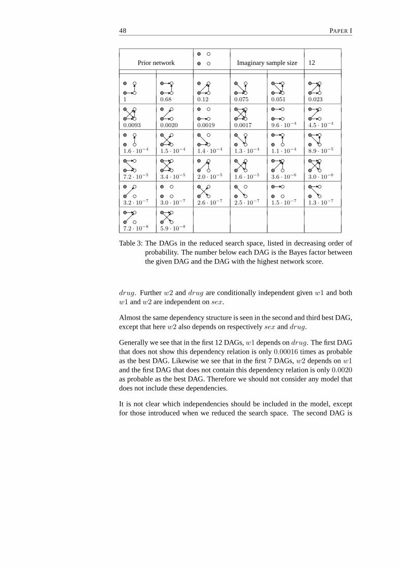
48 PAPER I
Prior network Imaginary sample size 12
1 0.68 0.12 0.075 0.051 0.023
0.0093 0.0020 0.0019 0.0017 9.6 · 10−4
4.5 · 10−4
1.6 · 10−4
1.5 · 10−4
1.4 · 10−4
1.3 · 10−4
1.1 · 10−4
8.9 · 10−5
7.2 · 10−5
3.4 · 10−5
2.0 · 10−5
1.6 · 10−5
3.6 · 10−6
3.0 · 10−6
3.2 · 10−7
3.0 · 10−7
2.6 · 10−7
2.5 · 10−7
1.5 · 10−7
1.3 · 10−7
7.2 · 10−8
5.9 · 10−8
Table 3: The DAGs in the reduced search space, listed in decreasing order ofprobability. The number below each DAG is the Bayes factor betweenthe given DAG and the DAG with the highest network score.
drug. Furtherw2 anddrug are conditionally independent givenw1 and bothw1 andw2 are independent onsex.
Almost the same dependency structure is seen in the second and third best DAG,except that herew2 also depends on respectivelysex anddrug.
Generally we see that in the first 12 DAGs,w1 depends ondrug. The first DAGthat does not show this dependency relation is only0.00016 times as probableas the best DAG. Likewise we see that in the first 7 DAGs,w2 depends onw1and the first DAG that does not contain this dependency relation is only0.0020as probable as the best DAG. Therefore we should not considerany model thatdoes not include these dependencies.
It is not clear which independencies should be included in the model, exceptfor those introduced when we reduced the search space. The second DAG is
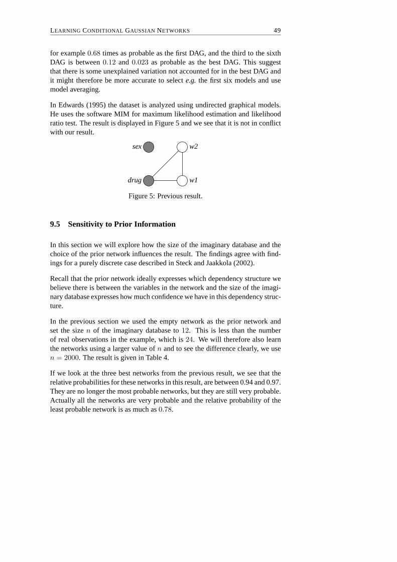
LEARNING CONDITIONAL GAUSSIAN NETWORKS 49
for example0.68 times as probable as the first DAG, and the third to the sixthDAG is between0.12 and 0.023 as probable as the best DAG. This suggestthat there is some unexplained variation not accounted for in the best DAG andit might therefore be more accurate to selecte.g. the first six models and usemodel averaging.
In Edwards (1995) the dataset is analyzed using undirected graphical models.He uses the software MIM for maximum likelihood estimation and likelihoodratio test. The result is displayed in Figure 5 and we see thatit is not in conflictwith our result.
sex
drug
w2
w1
Figure 5: Previous result.
9.5 Sensitivity to Prior Information
In this section we will explore how the size of the imaginary database and thechoice of the prior network influences the result. The findings agree with find-ings for a purely discrete case described in Steck and Jaakkola (2002).
Recall that the prior network ideally expresses which dependency structure webelieve there is between the variables in the network and thesize of the imagi-nary database expresses how much confidence we have in this dependency struc-ture.
In the previous section we used the empty network as the priornetwork andset the sizen of the imaginary database to12. This is less than the numberof real observations in the example, which is24. We will therefore also learnthe networks using a larger value ofn and to see the difference clearly, we usen = 2000. The result is given in Table 4.
If we look at the three best networks from the previous result, we see that therelative probabilities for these networks in this result, are between 0.94 and 0.97.They are no longer the most probable networks, but they are still very probable.Actually all the networks are very probable and the relativeprobability of theleast probable network is as much as0.78.

50 PAPER I
Prior network Imaginary sample size 2000
1 0.99 0.97 0.96 0.96 0.95
0.94 0.93 0.89 0.89 0.89 0.89
0.88 0.88 0.88 0.87 0.87 0.87
0.86 0.86 0.85 0.85 0.84 0.83
0.79 0.79 0.79 0.79 0.78 0.78
0.78 0.78
Table 4: The revised result with the prior network and the imaginary sample sizespecified as in the first line of this table.
The reason for this is that the prior network is the empty network, which repre-sents that all the variables are independent. This model is therefore a submodelof all other models. Whenn is large, we have much confidence in these inde-pendencies, so all networks will a priori be very probable. As the real databaseonly contains few observations, we have not enough information to differentiatebetween these networks and all the networks are therefore almost equally likely.
We will now explore what happens if we change the prior network. First we willlearn the structure using the most probable structure from Table 3 as the priornetwork. The results withn = 12 andn = 2000 are given in respectively Table5 and Table 6.
For n = 12 we see almost the same result as when using the empty network.The best networks are, not surprisingly, the same, only the order between themare a little different. To some extent, this also applies forn = 2000.

LEARNING CONDITIONAL GAUSSIAN NETWORKS 51
Prior network Imaginary sample size 12
1 0.59 0.38 0.34 0.17 0.10
0.064 0.056 2.7 · 10−4
1.3 · 10−4
1.2 · 10−4
4.8 · 10−5
4.5 · 10−5
2.2 · 10−5
1.9 · 10−5
7.9 · 10−6
7.5 · 10−8
5.0 · 10−8
4.4 · 10−8
2.9 · 10−8
2.9 · 10−8
2.6 · 10−8
1.9 · 10−8
1.7 · 10−8
2.1 · 10−11
1.4 · 10−11
9.9 · 10−12
8.9 · 10−12
6.5 · 10−12
5.8 · 10−12
3.6 · 10−12
2.4 · 10−12
Table 5: The revised result with the prior network and the imaginary sample sizespecified as in the first line of this table.
Further we see that for bothn = 12 andn = 2000, the 32 networks categorizeas follows. The8 networks with both arrowsdrug → w1 andw1→ w2 are the8 most probable networks. In the succeeding8 networks we havedrug → w1andw1 9 w2, after that the 8 networks withdrug 9 w1 andw1 → w2.In the last 8 networks we havedrug 9 w1 andw1 9 w2. Also we see thatwithin each category, the networks are almost equally likely, mostly pronouncedfor n = 2000. These finding are what we expected. The arrows included inthe prior network are all represented in the most probable networks and thesenetworks are all almost equally likely, as the prior networkis a submodel ofthese. Further there is a large difference in relative scorebetween the differentcategories, which shows that networks which include the arrowsdrug → w1andw1 → w2, are much more likely than those that do not. As this is validfor bothn = 12 andn = 2000, it is not only due to the influence of the priornetwork, but also because the dataset supports these dependencies.
We will now explore what happens if we choose the prior network to be the least

52 PAPER I
Prior network Imaginary sample size 2000
1 1 0.99 0.98 0.98 0.98
0.97 0.96 6.5 · 10−4
6.4 · 10−4
6.4 · 10−4
6.3 · 10−4
1.9 · 10−4
1.8 · 10−4
1.8 · 10−4
1.8 · 10−4
3.5 · 10−9
3.5 · 10−9
3.5 · 10−9
3.5 · 10−9
3.4 · 10−9
3.4 · 10−9
3.4 · 10−9
3.4 · 10−9
2.2 · 10−12
2.2 · 10−12
2.2 · 10−12
2.2 · 10−12
6.4 · 10−13
6.4 · 10−13
6.4 · 10−13
6.4 · 10−13
Table 6: The revised result with the prior network and the imaginary sample sizespecified as in the first line of this table.
probable network from Table 3. The results are forn = 12 andn = 2000 givenin respectively Table 7 and Table 8.
Forn = 12 we see almost the same result as with the other prior networks. Forn = 2000 we see that the8 most probable models actually are the8 modelsthat are possible with both the arrowssex → w1 andsex → w2. Further wesee that all networks are almost equally likely and there is not, as would beexpected, a large difference in score between networks withboth arrows and theothers. Actually for bothn = 12 andn = 2000 the result is very similar to theresult with the empty network as the prior networks. The reason for this is thatthe probability distribution of the prior network is estimated from data,i.e. weuse the sample mean and sample variance as the mean and variance in the priornetwork. If data does not support a dependence betweensex and respectivelyw1 andw2, then this prior network will be almost the same as the empty priornetwork and so will the result of the learning procedure. However, it can beseen that even small differences from the empty prior network have an impact

LEARNING CONDITIONAL GAUSSIAN NETWORKS 53
Prior network Imaginary sample size 12
1 0.25 0.13 0.094 0.023 0.012
0.0079 0.0020 0.0018 9.6 · 10−4
7.4 · 10−4
3.9 · 10−4
1.8 · 10−4
1.7 · 10−4
1.6 · 10−4
1.4 · 10−4
9.0 · 10−5
3.9 · 10−5
3.7 · 10−5
3.5 · 10−5
2.0 · 10−5
1.8 · 10−5
1.2 · 10−6
1.1 · 10−6
3.1 · 10−7
2.9 · 10−7
2.8 · 10−7
2.6 · 10−7
1.5 · 10−7
1.4 · 10−7
6.2 · 10−8
5.5 · 10−8
Table 7: The revised result with the prior network and the imaginary sample sizespecified as in the first line of this table.
whenn is large, as the8 most probable networks actually are the ones with bothsex→ w1 andsex→ w2.

54 PAPER I
Prior network Imaginary sample size 2000
1 0.99 0.94 0.94 0.91 0.90
0.86 0.86 0.67 0.65 0.61 0.59
0.59 0.59 0.54 0.53 0.38 0.37
0.35 0.35 0.34 0.33 0.32 0.31
0.25 0.25 0.22 0.22 0.22 0.22
0.20 0.20
Table 8: The revised result with the prior network and the imaginary sample sizespecified as in the first line of this table.
Acknowledgements
This research was supported by the ESPRIT project P29105 (BaKE). Also Iwould like to thank my supervisor Steffen L. Lauritzen for his dedicated helpand support.

LEARNING CONDITIONAL GAUSSIAN NETWORKS 55
References
Bernardo, J. M. and Smith, A. F. M. (1994).Bayesian Theory, John Wiley &Sons, Chichester.
Bøttcher, S. G. (2001). Learning Bayesian Networks with Mixed Variables,Ar-tificial Intelligence and Statistics 2001, Morgan Kaufmann, San Francisco,CA, USA, pp. 149–156.
Chickering, D. M. (1995). A transformational characterization of equivalentBayesian-network structures,Proceedings of Eleventh Conference on Un-certainty in Artificial Intelligence, Morgan Kaufmann, San Francisco, CA,USA, pp. 87–98.
Cooper, G. and Herskovits, E. (1992). A Bayesian method for the induction ofprobabilistic networks from data,Machine Learning9: 309–347.
Dawid, A. P. and Lauritzen, S. L. (1993). Hyper Markov laws inthe statisti-cal analysis of decomposable graphical models,The Annals of Statistics21(3): 1272–1317.
DeGroot, M. H. (1970). Optimal Statistical Decisions, McGraw-Hill, NewYork.
Edwards, D. (1995). Introduction to Graphical Modelling, Springer-Verlag,New York.
Frydenberg, M. (1990). Marginalization and collapsibility in graphical interac-tion models,Annals of Statistics18: 790–805.
Geiger, D. and Heckerman, D. (1994). Learning Gaussian Networks,Proceed-ings of Tenth Conference on Uncertainty in Artificial Intelligence, MorganKaufmann, San Francisco, CA, USA, pp. 235–243.
Heckerman, D., Geiger, D. and Chickering, D. M. (1995). Learning Bayesiannetworks: The combination of knowledge and statistical data, MachineLearning20: 197–243.
Lauritzen, S. L. (1992). Propagation of probabilities, means and variances inmixed graphical association models,Journal of the American StatisticalAssociation87(420): 1098–1108.
Lauritzen, S. L. (1996).Graphical Models, Clarendon press, Oxford, New York.
Lauritzen, S. L. and Jensen, F. (2001). Stable local computation with conditionalGaussian distributions,Statistics and Computing11: 191–203.
Morrison, D. F. (1976).Multivariate Statistical Methods, McGraw-Hill, USA.
Robinson, R. W. (1977). Counting unlabeled acyclic digraphs,Lecture Notes inMathematics, 622: Combinatorial Mathematics Vpp. 239–273.

56 PAPER I
Seber, G. A. F. (1984).Multivariate Observations, John Wiley and Sons, NewYork.
Shachter, R. D. and Kenley, C. R. (1989). Gaussian influence diagrams,Man-agement Science35: 527–550.
Spiegelhalter, D. J. and Lauritzen, S. L. (1990). Sequential updating of con-ditional probabilities on directed graphical structures,Networks20: 579–605.
Steck, H. and Jaakkola, T. S. (2002). On the Dirichlet Prior and Bayesian Regu-larization,Conference on Advances in Neural Information Processing Sys-tems, Vol. 15, MIT Press, Cambridge, USA.

Paper IIdeal: A Package for Learning
Bayesian Networks
Susanne G. Bøttcher and Claus Dethlefsen
Published in:Journal of Statistical Software(2003),
8(20):1-40.
57


deal: A Package for LearningBayesian Networks
Susanne G. Bøttcher
Aalborg University, Denmark
Claus Dethlefsen
Aalborg University, Denmark
Abstract.deal is a software package for use with R. It includes several methods for ana-lyzing data using Bayesian networks with variables of discrete and/or continuoustypes but restricted to conditionally Gaussian networks. Construction of priors fornetwork parameters is supported and their parameters can be learned from datausing conjugate updating. The network score is used as a metric to learn thestructure of the network and forms the basis of a heuristic search strategy. dealhas an interface to Hugin.
1 Introduction
A Bayesian network is a graphical model that encodes the joint probability dis-tribution for a set of random variables. Bayesian networks are treated ine.g.Cowell et al. (1999) and have found application within many fields, see Lau-ritzen (2003) for a recent overview.
Here we consider Bayesian networks with mixed variables,i.e. the random vari-ables in a network can be of both discrete and continuous types. A method forlearning the parameters and structure of such Bayesian networks has recentlybeen described by Bøttcher (2001). We have developed a package calleddeal,written in R (R Development Core Team 2003), which provides these methodsfor learning Bayesian networks. In particular, the packageincludes proceduresfor defining priors, estimating parameters, calculating network scores, perform-ing heuristic search as well as simulating data sets with a given dependencystructure. Figure 1 gives an overview of the functionality in deal. The pack-age can be downloaded from the ComprehensiveR Archive Network (CRAN)http://cran.R-project.org/ and may be used under the terms of the
59

60 PAPER II
GNU General Public License Version 2.
Figure 1: From prior knowledge and training data, a posterior network is pro-duced bydeal. The network may be transferred to Hugin for furtherinference.
In Section 2 we define Bayesian networks for mixed variables.To learn aBayesian network, the user needs to supply a training data set and representany prior knowledge available as a Bayesian network. Section 3 shows how tospecify the training data set indeal and Section 4 discusses how to specify aBayesian network in terms of a Directed Acyclic Graph (DAG) and the localprobability distributions.
deal uses the prior Bayesian network to deduce prior distributions for all pa-rameters in the model. Then, this is combined with the training data to yieldposterior distributions of the parameters. The parameter learning procedure istreated in Section 5.
Section 6 describes how to learn the structure of the network. A network scoreis calculated and a search strategy is employed to find the network with thehighest score. This network gives the best representation of data and we call ittheposterior network.
Section 7 describes how to transfer the posterior network toHugin (http://www.hugin.com). The Hugin graphical user interface (GUI) can then be

DEAL : A PACKAGE FOR LEARNING BAYESIAN NETWORKS 61
used for further inference in the posterior network.
In the appendix we provide manual pages for the main functions indeal.
2 Bayesian Networks
Let D = (V, E) be a Directed Acyclic Graph (DAG), whereV is a finite set ofnodes andE is a finite set of directed edges (arrows) between the nodes. TheDAG defines the structure of the Bayesian network.
To each nodev ∈ V in the graph corresponds a random variableXv. The set ofvariables associated with the graphD is thenX = (Xv)v∈V . Often, we do notdistinguish between a variableXv and the corresponding nodev. To each nodev with parents pa(v) a local probability distribution,p(xv|xpa(v)), is attached.The set of local probability distributions for all variables in the network isP.
A Bayesian network for a set of random variablesX is the pair(D,P).
The possible lack of directed edges inD encodes conditional independenciesbetween the random variablesX through the factorization of the joint probabil-ity distribution,
p(x) =∏
v∈V
p(
xv|xpa(v)
)
.
Here, we allow Bayesian networks with both discrete and continuous variables,as treated in Lauritzen (1992), so the set of nodesV is given byV = ∆ ∪ Γ,where∆ and Γ are the sets of discrete and continuous nodes, respectively.The set of variablesX can then be denotedX = (Xv)v∈V = (I, Y ) =((Iδ)δ∈∆, (Yγ)γ∈Γ), whereI andY are the sets of discrete and continuous vari-ables, respectively. For a discrete variable,δ, we letIδ denote the set of levels.
To ensuree.g.availability of exact local computation methods, we do not allowdiscrete variables to have continuous parents. The joint probability distributionthen factorizes into a discrete part and a mixed part, so
p(x) = p(i, y) =∏
δ∈∆
p(
iδ|ipa(δ))
∏
γ∈Γ
p(
yγ |ipa(γ), ypa(γ)
)
.

62 PAPER II
3 Data Structure
deal expects data as specified in a data frame which is a standard data structurein R. For example, standard ASCII data files with one column per variable andone line per observation can be read usingread.table()which returns a dataframe.
The rats example in Table 1 was constructed by Morrison (1976) and also stud-ied in Edwards (1995). The data set is from a hypothetical drug trial, where theweight losses of male and female rats under three different drug treatments havebeen measured after one and two weeks.
Sex Drug W1 W2M D1 5 6M D1 7 6M D1 9 9M D1 5 4M D2 9 12M D2 7 7M D2 7 6M D2 6 8M D3 14 11M D3 21 15M D3 12 10M D3 17 12F D1 7 10F D1 8 10F D1 6 6F D1 9 7F D2 7 6F D2 10 13F D2 6 9F D2 8 7F D3 14 9F D3 14 8F D3 16 12F D3 10 5
Table 1: An example data file,rats.dat.
The data are loaded into a data framerats.df by the following command
rats.df <- read.table("rats.dat",header=TRUE)
Before continuing, it is essential that the column variables have the correcttypes. Discrete variables should be specified asfactorsand continuous variablesasnumeric. To alter the type of a variable so that it is regarded as a discrete vari-able, use thefactor() function (standard inR). In the rats example,Sex and

DEAL : A PACKAGE FOR LEARNING BAYESIAN NETWORKS 63
Drug are interpreted to be factors byread.table, and thus no changes arenecessary.
We assume that we have observed complete data which means that noNA’s arepresent in the data frame.
4 Specification of a Bayesian Network
As described in Section 2, a Bayesian network is specified by aDAG and a setof local probability distributions. In this section we willshow how to specifythese terms indeal.
4.1 The Network Class and Associated Methods
In deal, a Bayesian network is represented as an object of classnetwork. Thenetwork object is a list of properties that are added or changed by the methodsdescribed in following sections.
A network is generated by the following command
rats <- network(rats.df)
and by default it is set to the empty network (the network without any arrows).
If the optionspecifygraph is set, a point and click graphical interface allowsthe user to insert and delete arrows until the requested DAG is obtained.
rats <- network(rats.df,specifygraph=TRUE)
A plot of the network (see Figure 2) is generated by
plot(rats)
Note that discrete nodes are grey and continuous nodes are white.
The primary property of a network is the list of nodes, in the example the list is:nodes(rats). Each entry in the list is an object of classnode representing a

64 PAPER II
Sex W2
Drug W1
Figure 2: Graphical representation of the rats network.
node in the graph, which includes information associated with the node. Severalmethods for the network class operate by applying an appropriate method forone or more nodes in the list of nodes. The nodes appear in the node list in thesame order as in the data frame used to create the network object.
It is possible to access the individual nodes in a network by referring either totheir index (the column number in the data frame) or to their name:
rats.nd <- nodes(rats)# the list of nodesrats.nd[[1]] # the first noderats.nd$Drug # the node ‘‘Drug’’
A collection of networks is represented in an object of classnetworkfamily,which has associatedprint() andplot() functions.
4.2 Specification of the Probability Distributions
The joint distribution of the random variables in a network in deal is a condi-tional Gaussian (CG) distribution.
For discrete nodes, this means that the local probability distributions are unre-stricted discrete distributions. We parameterize this as
θiδ |ipa(δ)= p(
iδ|ipa(δ), θδ|ipa(δ)
)
,
whereθδ|ipa(δ)= (θiδ|ipa(δ)
)iδ∈Iδ. The parameters fulfill
∑
iδ∈Iδθiδ |ipa(δ)
= 1and0 ≤ θiδ|ipa(δ)
≤ 1.
For continuous nodes, the local probability distributionsare Gaussian linear re-gressions on the continuous parents with parameters depending on the configu-ration of the discrete parents. We parameterize this as
θγ|ipa(γ)=(
mγ|ipa(γ), βγ|ipa(γ)
, σ2γ|ipa(γ)
)
,

DEAL : A PACKAGE FOR LEARNING BAYESIAN NETWORKS 65
so that
(
Yγ |ipa(γ), ypa(γ), θγ|ipa(γ)
)
∼ N(
mγ|ipa(γ)+ ypa(γ)βγ|ipa(γ)
, σ2γ|ipa(γ)
)
.
A suggestion for the local probability distributions is generated and attached toeach node as the propertyprob. The suggestion can then be edited afterwards.
For a discrete variableδ, the suggested local probability distributionp(iδ|ipa(δ))is taken to be uniform over the levels for each parent configuration,i.e.
p(iδ|ipa(δ)) = 1/Iδ.
Definezpa(γ) = (1, ypa(γ)) and letηγ|ipa(γ)= (mγ|ipa(γ)
, βγ|ipa(γ)), wheremγ|ipa(γ)
is the intercept andβγ|ipa(γ)is the vector of coefficients. For a continuous vari-
ableγ, the suggested local probability distribution
N (zpa(γ)ηγ|ipa(γ), σ2
γ|ipa(γ)),
is determined as a regression on the continuous parents for each configurationof the discrete parents.
The prob property for discrete nodes is a multi-way array with the node it-self occupying the first dimension and the parents each occupying one dimen-sion. For continuous nodes,σ2
γ|ipa(γ)andηγ|ipa(γ)
are stored in a matrix with one
row for each configuration of the discrete variables. The first column containsσ2
γ|ipa(γ)and the remaining columnsηγ|ipa(γ)
.
It is possible to inspect the suggested local probability distributions by settingthe optioninspectprob as
rats <- network(rats.df,inspectprob=TRUE)
This gives a graphical way of inspecting the local probability distribution byclicking on the nodes. Then, it is possible to adjust the local distributions,e.g.
localprob(rats,"Sex") <- c(0.6, 0.4)localprob(rats,"W1") <- c(10, 0)localprob(rats,"W2") <- c(10, 0, 1) # if eg. W2|W1

66 PAPER II
4.3 The Joint Distribution
We now show how the joint probability distribution of a network can be calcu-lated from the local probability distributions.
For the discrete part of the network, the joint probability distribution is found as
p(i) =∏
δ∈∆
p(
iδ|ipa(δ))
.
For continuous variables, the joint distributionN (Mi, Σi) is determined foreach configuration of the discrete variables by applying thefollowing sequentialalgorithm, see Shachter and Kenley (1989).
The order is determined so that the joint distribution of theparents have al-ready been determined for the current node. For notational convenience, weskip the indexi and determine the joint distribution of nodeγ and all previ-ously processed nodes,p. From the prior network, we have givenηγ|pa(γ) =(mγ|pa(γ), βγ|pa(γ)) andσ2
γ|pa(γ). Previously evaluated areMp andΣp. Now, thecovariance is given by
Σγ,p = Σp βγ|p,
whereβγ|p is a column vector of the regression coefficients given all previouslyevaluated nodes. All coefficients are zero, except the coefficients,βγ|pa(γ), cor-responding to the parents of the node. The variance and mean are then givenby
Σγ = σ2γ|pa(γ) + Σγ,p βγ|p
Mγ = mγ|pa(γ) + β⊤γ|p Mp.
In deal, we can assess these quantities by
rats.j <- jointprior(rats)
and inspect the propertiesjointmu, containingMi, jointsigma, containingΣi, andjointalpha. The discrete part,p(i), is not returned directly, but isfound by dividingrats.j$jointalpha with sum(rats.j$jointalpha).
DEAL : A PACKAGE FOR LEARNING BAYESIAN NETWORKS 67
5 Parameter Learning
In the previous section we showed how to specify a Bayesian network, i.e. aDAG and the local probability distributions. In this section we will show how toestimate the parameters in the local probability distributions from data. The firstsections present the theory behind the learning procedure and the last sectionshows how it is done indeal.
5.1 The Bayesian Approach
To estimate the parameters in the network, we use a Bayesian approach. Weencode our uncertainty about parametersθ in a prior distributionp(θ), use datad to update this distribution, and hereby obtain the posterior distributionp(θ|d)by using Bayes’ theorem,
p(θ|d) =p(d|θ)p(θ)
p(d), θ ∈ Θ. (1)
HereΘ is the parameter space,d is a random sample from the probability dis-tribution p(x|θ) andp(d|θ) is the joint probability distribution ofd, also calledthe likelihood ofθ. We refer to this asparameter learningor just learning.
In deal, we assume that the parameters associated with one variableare inde-pendent of the parameters associated with the other variables and, in addition,that the parameters are independent for each configuration of the discrete par-ents,i.e.
p(θ) =∏
δ∈∆
∏
ipa(δ)∈Ipa(δ)
p(θδ|ipa(δ))∏
γ∈Γ
∏
ipa(γ)∈Ipa(γ)
p(θγ|ipa(γ)). (2)
We refer to (2) asparameter independence. Further, as we have assumed com-plete data, the parameters stay independent given data, seeBøttcher (2001).This means that we can learn the parameters of a node independently of the pa-rameters of the other nodes,i.e.we update thelocal parameter priorp(θv|ipa(v)
)for each nodev and each configuration of the discrete parents.
As local prior parameter distributions, we use the Dirichlet distribution for thediscrete variables and the Gaussian-inverse gamma distribution for the contin-uous variables. These distributions are conjugate to observations from the re-spective distributions and this ensures simple calculations of the posterior dis-tributions.

68 PAPER II
In the next section we present an automated procedure for specifying the localparameter priors associated with any possible DAG. The procedure is called themaster prior procedure. For the mixed case it is treated in Bøttcher (2001), forthe purely discrete and the purely continuous cases it is treated in Heckerman etal. (1995) and Geiger and Heckerman (1994), respectively.
5.2 The Master Prior Procedure
In the following sections we will show how to deduce and update the local priorparameter distributions for discrete and continuous nodes, respectively. Here,we will summarize the steps in the master prior procedure.
The idea is that from a given Bayesian network, we can deduce parameter priorsfor any possible DAG. The user just has to specify the Bayesian network as hebelieves it to be. We call this network aprior Bayesian network.
1. Specify a prior Bayesian network,i.e. a prior DAG (Section 4.1) and priorlocal probability distributions (Section 4.2). Calculatethe joint prior distri-bution (Section 4.3).
2. From this joint prior distribution, the marginal distribution of all parametersin the family consisting of the node and its parents can be determined. Wecall this themaster prior.
3. The local parameter priors are now determined by conditioning in the mas-ter prior distribution.
This procedure ensures parameter independence. Further, it has the property thatif a node has the same set of parents in two different networks, then the localparameter prior for this node will be the same in the two networks. Therefore,we only have to deduce the local parameter prior for a node given the same setof parents once. This property is calledparameter modularity.
5.3 Discrete Nodes
We will now show how to find the local parameter priors for the discrete nodes.Recall that the local probability distributions are unrestricted discrete distribu-tions defined as in Section 4.2.

DEAL : A PACKAGE FOR LEARNING BAYESIAN NETWORKS 69
Master Prior
Let Ψ = (Ψi)i∈I be the parameters for the joint distribution of the discretevariables. The joint prior parameter distribution is assumed to be a Dirichletdistribution
p(Ψ) ∼ D(α),
with hyperparametersα = (αi)i∈I . To specify this Dirichlet distribution, weneed to specify these hyperparameters.
Consider the following relation for the Dirichlet distribution,
p(i) = E(Ψi) =αi
N,
with N =∑
i∈I αi. Now we use the probabilities in the prior network as anestimate ofE(Ψi), so we only need to determineN in order to calculate theparametersαi.
We determineN by using the notion of an imaginary data base. We imagine thatwe have a data base of cases, from which we have updated the distribution ofΨout of total ignorance. Theimaginary sample sizeof this imaginary data baseis thusN . It expresses how much confidence we have in the (in)dependenciesexpressed in the prior network, see Heckerman et al. (1995).
We use this joint distribution to deduce the master prior distribution of the familyA = δ ∪ pa(δ). Let
αiA =∑
j:jA=iA
αj ,
and letαA = (αiA)iA∈IA. Then the marginal distribution ofΨA is Dirichlet,
p(ΨA) ∼ D(αA). This is the master prior in the discrete case.
Local Parameter Prior
From the master prior, we calculate the conditional distribution Ψδ|ipa(δ)=
θδ|ipa(δ)which is the local parameter prior in the discrete case. Then,
αiδ|ipa(δ)= αiA ,
αδ|ipa(δ)=(
αiδ |ipa(δ)
)
iδ∈Iδ,
θδ|ipa(δ)|αiδ|ipa(δ)
∼ D(
αδ|ipa(δ)
)
.

70 PAPER II
Local Parameter Posterior
Let nδ|ipa(δ)be the number of cases observed with the particular parent configu-
ration in the data base and letn be the total number of observations.
Then, the posterior parametersα′δ|ipa(δ)
are given by
α′δ|ipa(δ)
= αδ|ipa(δ)+ nδ|ipa(δ)
.
5.4 Continuous Nodes
We now show how to find the local parameter priors for the continuous nodes.Recall that the local probability distributions are normaldistributions defined asin Section 4.2.
Master Prior
Bøttcher (2001) derived this procedure in the mixed case. For a configurationi of the discrete variables we letνi = ρi = αi, whereαi was determined inSection 5.3. Also,Φi = (νi − 1)Σi.
The joint parameter priors are assumed to be distributed as
p(Mi|Σi) = N
(
µi,1
νiΣi
)
,
p(Σi) = IW (ρi, Φi),
whereIW is the inverse Wishart distribution.
However, since the marginal distribution of a CG distribution is not necessarilya CG distribution, there is no simple way to derive priors forother networks.Instead we use the imaginary data base to derive local masterpriors.
Define the notation
ρiA∩∆ =∑
j:jA∩∆=iA∩∆
ρj
and similarly forνiA∩∆ andΦiA∩∆ . For the familyA = γ ∪ pa(γ), the local

DEAL : A PACKAGE FOR LEARNING BAYESIAN NETWORKS 71
master prior is then found as
ΣA∩Γ|iA∩∆∼ IW
(
ρiA∩∆ , ΦA∩Γ|iA∩∆
)
,
MA∩Γ|iA∩∆|ΣA∩Γ|iA∩∆
∼ N
(
µA∩Γ|iA∩∆,
1
νiA∩∆
ΣA∩Γ|iA∩∆
)
,
where
µiA∩∆ =
∑
j:jA∩∆=iA∩∆µjνj
νiA∩∆
,
ΦA∩Γ|iA∩∆= ΦiA∩∆ +
∑
j:jA∩∆=iA∩∆
νj(µj − µiA∩∆)(µj − µiA∩∆)⊤.
Local Parameter Prior
UsingIΓ for the inverse gamma distribution, the local prior parameters, givenas
(
mγ|ipa(γ), βγ|ipa(γ)
| σ2γ|ipa(γ)
)
∼ N(
µγ|ipa(γ), σ2
γ|ipa(γ)τ−1γ|ipa(γ)
)
,
σ2γ|ipa(γ)
∼ IΓ
(
ργ|ipa(γ)
2,φγ|ipa(γ)
2
)
,
are deduced from the local master prior by conditioning as follows. To sim-plify notation, we ignore all subscripts in the master priorand thus consider theconfigurationiA∩∆ = ipa(γ) and assume thatA ∩ Γ is ordered withγ as thefirst entry. Write pa(γ) for the continuous parents{A ∩ Γ} \ {γ}. Define thepartitioning
ΦA∩Γ|iA∩∆=
[
φγ Φγ,pa(γ)
Φpa(γ),γ Φpa(γ)
]
,
µiA∩∆ =
(
µγ , µpa(γ)
)
.
Then
µγ|ipa(γ)=
(
µγ − Φγ,pa(γ)Φ−1pa(γ)µpa(γ) , Φγ,pa(γ)Φ
−1pa(γ)
)
,
φγ|ipa(γ)= φγ − Φγ,pa(γ)Φ
−1pa(γ)Φpa(γ),γ ,
ργ|ipa(γ)= ρiA∩∆ + |pa(γ)|,
τγ|ipa(γ)=
(
1/νiA∩∆ + µ⊤pa(γ)Φ
−1pa(γ)µpa(γ) −µ⊤
pa(γ)Φ−1pa(γ),
−Φ−1pa(γ)µpa(γ) Φ−1
pa(γ)
)−1
.

72 PAPER II
Local Parameter Posterior
Define zbpa(γ)|ipa(γ)
as the matrix withn rows and with a column of ones and
columns of the observed continuous parents for a given configuration of thediscrete parents. Letyb
γ|ipa(γ)be the vector of observations of the nodeγ for a
configuration of the discrete parents.
Then, the prior parametersτγ|ipa(γ), µγ|ipa(γ)
, ργ|ipa(γ), φγ|ipa(γ)
are updated toposterior parameters (denoted with a prime) by the following relations
τ ′γ|ipa(γ)
= τγ|ipa(γ)+(
zbpa(γ)|ipa(γ)
)⊤zb
pa(γ)|ipa(γ),
µ′γ|ipa(γ)
=(
τ ′γ|ipa(γ)
)−1×
(
τγ|ipa(γ)µγ|ipa(γ)
+ (zbpa(γ)|ipa(γ)
)⊤ybγ|ipa(γ)
)
,
ρ′γ|ipa(γ)= ργ|ipa(γ)
+ n,
φ′γ|ipa(γ)
= φγ|ipa(γ)
+(
ybγ|ipa(γ)
− zbpa(γ)µ
′γ|ipa(γ)
)⊤yb
γ|ipa(γ)
+(
µγ|ipa(γ)− µ′
γ|ipa(γ)
)⊤τγ|ipa(γ)
µγ|ipa(γ).
5.5 The Learning Procedure indeal
Assume that the training data are available in a data frame,rats.df, as de-scribed in Section 3. Also, assume that the user has specifieda Bayesian net-work to be used as prior network, calledrats, see Section 4.
The parameters of the joint distribution of the variables inthe network are thendetermined by the functionjointprior() with the size of the imaginary database as optional argument. If the size is not specified,deal sets the size to areasonably small value.
rats.prior <- jointprior(rats)## auto set size of imaginary data base
rats.prior <- jointprior(rats,12)## set size of imaginary data base to 12
The parameters in the objectrats.prior may be assessed as

DEAL : A PACKAGE FOR LEARNING BAYESIAN NETWORKS 73
rats.prior$jointalpharats.prior$jointnurats.prior$jointrhorats.prior$jointphi
The procedurelearn() determines the master prior, local parameter priors andlocal parameter posteriors and may be called on all nodes or just a single node.The result is accessed using thegetnetwork() extractor function.
rats <- getnetwork(learn(rats,rats.df,rats.prior))## all nodes
rats <- getnetwork(learn(rats,rats.df,rats.prior,2))## only node 2
In the result, each learned node has now attached two properties. These containthe parameters in the local prior distribution and the parameters in the localposterior distribution, respectively. For the nodeSex, the properties are assessedas
localprior(nodes(rats)$Sex)localposterior(nodes(rats)$Sex)
6 Learning the Structure
In this section we will show how to learn the structure of the DAG from data.The section is based on Bøttcher (2001), Heckerman et al. (1995) and Geigerand Heckerman (1994).
6.1 Network Score
As a measure of how well a DAGD represents the conditional independenciesbetween the random variables, we use the relative probability
S(D) = p(D, d) = p(d|D)p(D),
and refer to it as anetwork score.
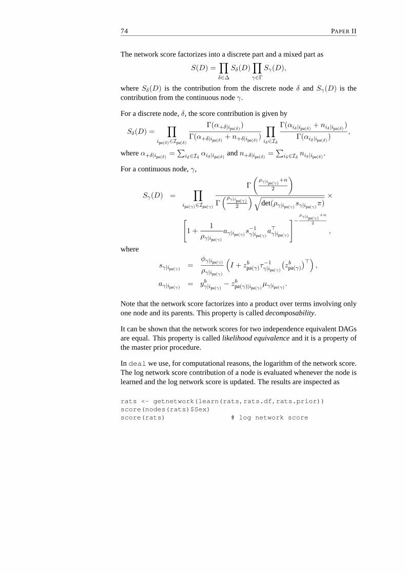
74 PAPER II
The network score factorizes into a discrete part and a mixedpart as
S(D) =∏
δ∈∆
Sδ(D)∏
γ∈Γ
Sγ(D),
whereSδ(D) is the contribution from the discrete nodeδ and Sγ(D) is thecontribution from the continuous nodeγ.
For a discrete node,δ, the score contribution is given by
Sδ(D) =∏
ipa(δ)∈Ipa(δ)
Γ(α+δ|ipa(δ))
Γ(α+δ|ipa(δ)+ n+δ|ipa(δ)
)
∏
iδ∈Iδ
Γ(αiδ|ipa(δ)+ niδ|ipa(δ)
)
Γ(αiδ|ipa(δ))
,
whereα+δ|ipa(δ)=∑
iδ∈Iδαiδ |ipa(δ)
andn+δ|ipa(δ)=∑
iδ∈Iδniδ |ipa(δ)
.
For a continuous node,γ,
Sγ(D) =∏
ipa(γ)∈Ipa(γ)
Γ
(
ργ|ipa(γ)+n
2
)
Γ(ργ|ipa(γ)
2
)√
det(ργ|ipa(γ)sγ|ipa(γ)
π)×
[
1 +1
ργ|ipa(γ)
aγ|ipa(γ)s−1γ|ipa(γ)
a⊤γ|ipa(γ)
]−ργ|ipa(γ)
+n
2
,
where
sγ|ipa(γ)=
φγ|ipa(γ)
ργ|ipa(γ)
(
I + zbpa(γ)τ
−1γ|ipa(γ)
(
zbpa(γ)
)⊤)
,
aγ|ipa(γ)= yb
γ|ipa(γ)− zb
pa(γ)|ipa(γ)µγ|ipa(γ)
.
Note that the network score factorizes into a product over terms involving onlyone node and its parents. This property is calleddecomposability.
It can be shown that the network scores for two independence equivalent DAGsare equal. This property is calledlikelihood equivalenceand it is a property ofthe master prior procedure.
In deal we use, for computational reasons, the logarithm of the network score.The log network score contribution of a node is evaluated whenever the node islearned and the log network score is updated. The results areinspected as
rats <- getnetwork(learn(rats,rats.df,rats.prior))score(nodes(rats)$Sex)score(rats) # log network score

DEAL : A PACKAGE FOR LEARNING BAYESIAN NETWORKS 75
6.2 Model Search
In principle, we could evaluate the network score for all possible DAGs andindeed this is provided indeal.
allrats <- networkfamily(rats.df,rats,rats.prior)allrats <- nwfsort(getnetwork(allrats))
However, the number of possible DAGs grows more than exponentially withthe number of nodes (see Table 2) and, in general, the problemof identifyingthe network with the highest score is NP-complete (see Chickering (1996)). If
# nodes # networks1 12 2–33 12–254 144–5435 4800–292816 320000–37815037 ≈ 56 · 106 – 109
8 ≈ 1010 – 1011
9 ≈ 1013 – 1015
10 ≈ 1016 – 1018
Table 2: The (approximate) number of networks for a given number of nodes.Since we do not allow arrows from continuous to discrete nodes, thenumber of networks for a given number of nodes is given as a lowerand upper bound.
the number of random variables in a network is large, it is notcomputationallypossible to calculate the network score for all the possibleDAGs. For thesesituations a strategy for searching for DAGs with high scoreis needed. Indeal,the search strategygreedy search with random restarts, see Heckerman et al.(1995), is implemented. As a way of comparing the network scores for twodifferent DAGs,D andD∗, we use the posterior odds,
p(D|d)
p(D∗|d)=
p(D, d)
p(D∗, d)=
p(D)
p(D∗)×
p(d|D)
p(d|D∗),
wherep(D)/p(D∗) is the prior odds andp(d|D)/p(d|D∗) is the Bayes factor.At the moment, the only option indeal for specifying prior distribution over

76 PAPER II
DAGs is to let all DAGs be equally likely, so the prior odds arealways equal toone. Therefore, we use the Bayes factor for comparing two different DAGs.
In greedy search we compare models that differ only by a single arrow, eitheradded, removed or reversed. In these cases, the Bayes factoris especially sim-ple, because of decomposability of the network score.
Greedy search works as follows.
1. Select an initial DAGD0, from which to start the search.
2. Calculate Bayes factors betweenD0 and all possible networks, which differby only one arrow, that is
(a) One arrow is added toD0.
(b) One arrow inD0 is deleted.
(c) One arrow inD0 is turned.
3. Among all these networks, select the one that increases the Bayes factorthe most.
4. If the Bayes factor is not increased, stop the search. Otherwise, let thechosen network beD0 and repeat from 2.
In deal
rats.s <- getnetwork(autosearch(rats,rats.df,rats.prior))
returns all tried networks in a greedy search from the initial network rats,which may be constructed usingdrawnetwork().
Sex W2
Drug W1
Figure 3: The network with the highest score in the rats example.
To manually assess the network score of a network (e.g.to use as initial networkin a search), use
rats <- getnetwork(drawnetwork(rats,rats.df,rats.prior))

DEAL : A PACKAGE FOR LEARNING BAYESIAN NETWORKS 77
In the drawnetwork() procedure, it is possible to mark (ban) some of thearrows. In the search,deal then disregards any DAG which contains any ofthese arrows, and this reduces the search space.
The search algorithm may also be used with restarts which is implemented inthe functionheuristic(). The initial network is then perturbed according tothe parameterdegree and the search is performed starting with the perturbednetwork. The process is restarted the number of times specified by the optionrestart. A network family of all visited networks is returned.
rats.h <- getnetwork(heuristic(rats,rats.df,rats.prior,restart=10,degree=5))
The perturbation of the initial network is done as follows
1. Randomly choose between one of three actions(a) Insert an arrow.(b) Delete an arrow.(c) Turn an arrow.
2. After selection of the action, perform the action according toInsert Choose randomly between all possible insertions of one arrow.Delete Choose randomly between all possible deletions of one arrow.Turn Choose randomly between all possible turns of one arrow.If the action is not possible, return the unchanged network.
Perturbation is done automatically inheuristic() by calling the functionperturb(). However, a random graph may also be generated by directly call-ing perturb()
rats.rn <- getnetwork(perturb(rats,rats.df,rats.prior,degree=10))
6.3 Using Equivalence Relations to Speed up Model Search
In Bøttcher (2003) two types of equivalences are identified and it is shown thatno other equivalences exist. LetD1 andD∗
1 be two different networks that differby a single arrow between the nodesv andw, with v ← w in D1 andv 8 win D∗
1. Further, letD2 andD∗2 be another two networks that differ by an arrow
betweenv andw.

78 PAPER II
1. The Bayes factor for testing the arrow fromv to w is equivalent to testingthis arrow in any other network, wherev has the same parents as inD1.
2. The Bayes factor for testing the arrow fromv to w is equivalent to thisarrow in the network, wherew has the same parents inD2 asv has inD1,with the exception thatv is also a parent ofw in D2.
We use the first equivalence in all functions that call the learning procedure, in-cludingheuristic(), learn(), drawnetwork(), networkfamily() andperturb(), by maintaining a so-calledtrylist. Thetrylist may be givenas input to the functions and is returned in an updated version.
Thetrylist contains a list for each node in the network. The list for a nodeconsists of the result after learning the node for all parentconfigurations thathas previously been tried. When a node is learned after a change in its parentstructure, we first look in thetrylist to see if the node has been learned beforewith the same parent configuration (Equivalence 1). If the equivalence cannot beused, the node is learned and the result is inserted in thetrylist. Utilizationof Equivalence 2 is not yet implemented indeal.
The cost of looking in thetrylist is smaller than learning a node. Note,however, that thetrylist must be recalculated if the imaginary data base sizeis changed or if the data base is changed.
In deal, there is support for generating the completetrylist, that is, allnodes are learned with all possible parent configurations.
rats.tl <- maketrylist(rats,rats.df,rats.prior)rats.h <- getnetwork(heuristic(rats,rats.df,rats.prior,
trylist=rats.tl))
7 Hugin Interface
A network object may be written to a file in the Hugin.net language. Hugin(http://www.hugin.com) is commercial software for inference in Bayes-ian networks. Hugin has the ability to learn networks with only discrete vari-ables, but cannot learn either purely continuous or mixed networks.deal maytherefore be used for this purpose and the result can then be transferred to Hugin.
The proceduresavenet() saves a network to a connection (for example a file).

DEAL : A PACKAGE FOR LEARNING BAYESIAN NETWORKS 79
For each node, we use point estimates of the parameters in thelocal probabilitydistributions.
Thereadnet() procedure reads the network structure from a connection butdoes not, however, read the probability distributions. This is planned to be in-cluded in a future version ofdeal.
8 Example
In this section,deal is used to analyze a large data set which includes bothdiscrete and continuous variables. Theksldata set, included in Badsberg (1995),is from a study measuring health and social characteristicsof representativesamples of Danish 70-year old people, taken in 1967 and 1984.In total, 1083cases have been recorded and each case contains observations on nine differentvariables, see Table 3.
Node index Variable Explanation1 Fev Forced ejection volume – lung function2 Kol Cholesterol3 Hyp Hypertension (no/yes)4 BMI Body Mass Index5 Smok Smoking (no/yes)6 Alc Alcohol consumption (seldom/frequently)7 Work Working (yes/no)8 Sex Gender (male/female)9 Year Survey year (1967/1984)
Table 3: Variables in theksl data set. The variablesFev, Kol, BMI are continu-ous variables and the rest are discrete variables.
The purpose of our analysis is to find dependency relations between the vari-ables. One interest is to determine which variables influence the presence orabsence of hypertension. From a medical viewpoint, it is possible that hyper-tension is influenced by some of the continuous variablesFev, Kol andBMI.However, indeal we do not allow continuous parents of discrete nodes, so wecannot describe such a relation. A way to overcome this problem is to treatHypas a continuous variable, even though this is obviously not most natural. This isdone in the analysis below.

80 PAPER II
Further, the initial data analysis indicates a transformation ofBMI into log(BMI).With these adjustments, the data set is ready for analysis indeal.
First,deal is activated and the data are read into a data frame and prepared foranalysis.
library(deal) ## invoke DEAL
data(ksl) ## read data (included in DEAL)
The next step in the analysis is to specify a prior Bayesian network. We haveno prior knowledge about specific dependency relations, so for simplicity weuse the empty DAG as the prior DAG and let the probability distribution of thediscrete variables be uniform. The assessment of the probability distribution forthe continuous variables is based on data, as described in Section 4.2.
## specify prior networkksl.nw <- network(ksl)
## make joint prior distributionksl.prior <- jointprior(ksl.nw)
We do not allow arrows into Sex and Year, as none of the other variables can in-fluence these variables. So we create a ban list which is attached to the network.The ban list is a matrix with two columns. Each row contains the directed edgethat is not allowed. The ban list could also have been createdinteractively usingthe functiondrawnetwork().
## ban arrows towards Sex and Yearmybanlist <- matrix(c(5,5,6,6,7,7,9,
8,9,8,9,8,9,8),ncol=2)banlist(ksl.nw) <- mybanlist
Finally, the parameters in the network are learned and structural learning is ini-tiated usingautosearch() and heuristic(). We use the prior DAG asstarting point for the structural search.

DEAL : A PACKAGE FOR LEARNING BAYESIAN NETWORKS 81
## learn the initial networkksl.nw <- getnetwork(learn(ksl.nw,ksl,ksl.prior))
## Do structural searchksl.search <- autosearch(ksl.nw,ksl,ksl.prior,trace=TRUE)
## perturb ’thebest’ and rerun search twice.ksl.heuristic <- heuristic(getnetwork(ksl.search),
ksl,ksl.prior,restart=2,degree=10,trace=TRUE,trylist=gettrylist(ksl.search))
thebest2 <- getnetwork(ksl.heuristic)
savenet(thebest2, file("ksl.net"))
FEV
Kol
Hyp
logBMI
SmokAlc
Work
Sex
Year
Figure 4: The network with the highest score,log(score) = −15957.91.
The resulting networkthebest2 is shown in Figure 4 and it is the network withthe highest network score among those networks that have been tried throughthe search.
In the result we see for the discrete variables thatAlc, Smok andWork dependdirectly onSex andYear. In addition,Smok andWork also depend onAlc.

82 PAPER II
These two arrows are, however, not causal arrows, asSmok ← Alc → Work
in the given DAG represents the same probability distribution as the relationsSmok ← Alc ← Work andSmok → Alc → Work, i.e. the three DAGs areindependence equivalent.
Year andSex are independent on all variables, as specified in the ban list.
For the continuous variables all the arrows are causal arrows. We see thatFevdepends directly onYear, Sex andSmok. So given these variables,Fev isconditionally independent on the rest of the variables.Kol depends directly onYear andSex, andlogBMI depends directly onKol andSex.
GivenlogBMI andFev, the variableHyp is conditionally independent on therest of the variables. So according to this study, hypertension can be determinedby the body mass index and the lung function forced ejection volume. However,asHyp is not continuous by nature, other analyses should be performed withHyp as a discrete variable,e.g. a logistic regression withHyp as a responseand the remaining as explanatory variables. Such an analysis indicates that, inaddition,Sex andSmok may influenceHyp, but otherwise identifieslogBMI asthe main predictor.
9 Discussion and Future Work
deal is a tool box that adds functionality toR so that Bayesian networks maybe used in conjunction with other statistical methods available inR for analyz-ing data. In particular,deal is part of the gR project, which is a newly initiatedworkgroup with the aim of developing procedures inR for supporting data anal-ysis with graphical models, seehttp://www.r-project.org/gR.
In addition to methods for analyzing networks with either discrete or continuousvariables,deal handles networks with mixed variables.
deal has some limitations and we plan to extend the package with the proce-dures described below. Also, it is the intention that the procedures indeal willeventually be adjusted to the other procedures developed under the gR project.
The methods indeal are only applicable on complete data sets and in thefuture, we would like to incorporate procedures for handling data with missingvalues and networks with latent variables.

DEAL : A PACKAGE FOR LEARNING BAYESIAN NETWORKS 83
The criteria for comparing the different network structures indeal, is the rela-tive probabilityS(D). We intend to also incorporate the Bayesian InformationCriteria (BIC) and Akaikes Information Criteria (AIC) and let it be up to theuser to decide which criteria to use.
Another possible extension ofdeal is to incorporate procedures for specifyingmixed networks, where the variance in the mixed part of the network does notdepend on the discrete parents, but the mean does.
Finally, we are working on an implementation of the greedy equivalence search(GES) algorithm, see Chickering (2002), which is an algorithm for search be-tween equivalence classes. Asymptotically, for the size ofthe database tendingto infinity, this algorithm guarantees that the search terminates with the networkwith the highest network score.
Acknowledgements
The work has been supported by Novo Nordisk A/S. We thank the reviewer formany helpful comments.
References
Badsberg, J. H. (1995).An Environment for Graphical Models, PhD thesis,Aalborg University.
Bøttcher, S. G. (2001). Learning Bayesian Networks with Mixed Variables,Ar-tificial Intelligence and Statistics 2001, Morgan Kaufmann, San Francisco,CA, USA, pp. 149–156.
Bøttcher, S. G. (2003). Learning Bayesian networks with mixed variables, Aal-borg University,http://www.math.auc.dk/~alma.
Chickering, D. M. (1996). Learning Bayesian networks is NP-Complete,inD. Fisher and H. J. Lenz (eds),Learning from Data: Artificial Intelligenceand Statistics V, Springer-Verlag, New York, pp. 121–130.
Chickering, D. M. (2002). Optimal structure identificationwith greedy search,Journal of Machine Learning Research3: 507–554.
Cowell, R. G., Dawid, A. P., Lauritzen, S. L. and Spiegelhalter, D. J. (1999).Probabilistic Networks and Expert Systems, Springer-Verlag, Berlin-Heidelberg-New York.

84 PAPER II
Edwards, D. (1995). Introduction to Graphical Modelling, Springer-Verlag,New York.
Geiger, D. and Heckerman, D. (1994). Learning Gaussian Networks,Proceed-ings of Tenth Conference on Uncertainty in Artificial Intelligence, MorganKaufmann, San Francisco, CA, USA, pp. 235–243.
Heckerman, D., Geiger, D. and Chickering, D. M. (1995). Learning Bayesiannetworks: The combination of knowledge and statistical data, MachineLearning20: 197–243.
Lauritzen, S. L. (1992). Propagation of probabilities, means and variances inmixed graphical association models,Journal of the American StatisticalAssociation87(420): 1098–1108.
Lauritzen, S. L. (2003). Some modern applications of graphical models,in P. J.Green, N. L. Hjort and S. Richardson (eds),Highly Structured StochasticSystems, Oxford University Press, Oxford, pp. 13–32.
Morrison, D. F. (1976).Multivariate Statistical Methods, McGraw-Hill, USA.
R Development Core Team (2003).R: A language and environment for statis-tical computing, R Foundation for Statistical Computing, Vienna, Austria.ISBN 3-900051-00-3.
Shachter, R. D. and Kenley, C. R. (1989). Gaussian influence diagrams,Man-agement Science35: 527–550.
10 Manual Pages fordeal
autosearch Greedy search
Description
From initial network, does local perturbations to increasenetwork score.
Usage
autosearch(initnw,data,prior=jointprior(network(data)),maxiter=50,trylist= vector("list",size(initnw)),trace=TRUE,timetrace=TRUE,showban=FALSE,removecycles=FALSE)
heuristic(initnw,data,prior=jointprior(network(data)),maxiter=100,restart=10,degree=size(initnw),

DEAL : A PACKAGE FOR LEARNING BAYESIAN NETWORKS 85
trylist= vector("list",size(initnw)),trace=TRUE,timetrace=TRUE,removecycles=FALSE)
gettable(x)
Arguments
initnw an object of classnetwork, from which the search is started.data a data frame used for learning the network, seenetwork.prior a list containing parameter priors, generated byjointprior.maxiter an integer, which gives the maximum number of steps in the search algorithm.restart an integer, which gives the number of times to perturbinitnw and rerun the
search.degree an integer, which gives the degree of perturbation, seeperturb.trylist a list used internally for reusing learning of nodes, seemaketrylist.trace a logical. IfTRUE, plots the accepted networks during search.timetrace a logical. IfTRUE, prints some timing information on the screen.showban a logical passed to the plot method for network objects. IfFALSE, the banned
arrows are not shown in the plots (iftrace is TRUE).removecycles a logical. IfTRUE, all networks explored in the search is returned, except for
networks containing a cycle. IfFALSE, all networks are returned, includingcyclic networks.
x an output object from a search.
Details
In autosearch, a list of networks is in each step created with either one arrow added, one arrowdeleted or one arrow turned (if a cycle is not generated). Thenetwork scores of all the proposal networksare calculated and the network with the highest score is chosen for the next step in the search. If noproposed network has a higher network score than the previous network, the search is terminated. Thenetwork with the highest network score is returned, along with a list containing all tried networks(depending on the value ofremovecycles).heuristic restarts by perturbinginitnw degree times and callingautosearch again. Thenumber of restarts is given by the optionrestart.
Value
autosearch andheuristic returns a list with three elements, that may be accessed using thefunctionsgetnetwork, gettable andgettrylist. The elements arenw an object of classnetwork, which gives the network with the highest score.table a table with all tried networks. If removecycles isFALSE, the networks may
contain cycles. The table contains two columns:model with a string repre-sentation of the model andscore with the corresponding log network score.The table can be translated to anetworkfamily usingmakenw.
trylist an updated list used internally for reusing learning of nodes, seemaketrylist.
Author(s)
Susanne Gammelgaard Bøttcher〈[email protected]〉,Claus Dethlefsen〈[email protected]〉.
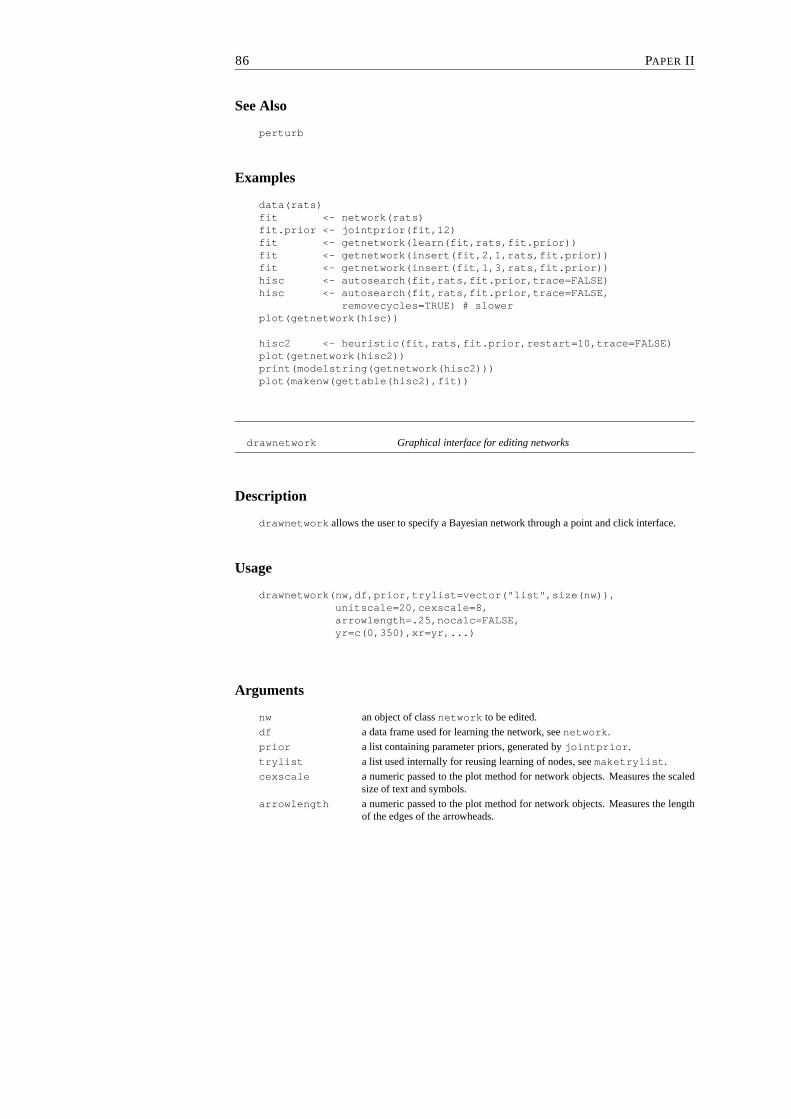
86 PAPER II
See Also
perturb
Examples
data(rats)fit <- network(rats)fit.prior <- jointprior(fit,12)fit <- getnetwork(learn(fit,rats,fit.prior))fit <- getnetwork(insert(fit,2,1,rats,fit.prior))fit <- getnetwork(insert(fit,1,3,rats,fit.prior))hisc <- autosearch(fit,rats,fit.prior,trace=FALSE)hisc <- autosearch(fit,rats,fit.prior,trace=FALSE,
removecycles=TRUE) # slowerplot(getnetwork(hisc))
hisc2 <- heuristic(fit,rats,fit.prior,restart=10,trace=FALSE)plot(getnetwork(hisc2))print(modelstring(getnetwork(hisc2)))plot(makenw(gettable(hisc2),fit))
drawnetwork Graphical interface for editing networks
Description
drawnetwork allows the user to specify a Bayesian network through a pointand click interface.
Usage
drawnetwork(nw,df,prior,trylist=vector("list",size(nw)),unitscale=20,cexscale=8,arrowlength=.25,nocalc=FALSE,yr=c(0,350),xr=yr,...)
Arguments
nw an object of classnetwork to be edited.
df a data frame used for learning the network, seenetwork.prior a list containing parameter priors, generated byjointprior.
trylist a list used internally for reusing learning of nodes, seemaketrylist.cexscale a numeric passed to the plot method for network objects. Measures the scaled
size of text and symbols.
arrowlength a numeric passed to the plot method for network objects. Measures the lengthof the edges of the arrowheads.
DEAL : A PACKAGE FOR LEARNING BAYESIAN NETWORKS 87
nocalc a logical. IfTRUE, no learning procedure is called, see eg.rnetwork.
unitscale a numeric passed to the plot method for network objects. Scale parameter forchopping off arrow heads.
xr a numeric vector with two components containing the range onx-axis.
yr a numeric vector with two components containing the range ony-axis.
... additional plot arguments, passed to the plot method for network objects.
Details
To insert an arrow from node ’A’ to node ’B’, first click node ’A’ and then click node ’B’. When thegraph is finished, click ’stop’.To specify that an arrow must not be present, press ’ban’ (a toggle) and draw the arrow. This is shownas a red dashed arrow. It is possible to ban both directions between nodes. The ban list is stored withthe network in the propertybanlist. It is a matrix with two columns. Each row is the ’from’ nodeindex and the ’to’ node index, where the indices are the column number in the data frame.Note that the network score changes as the network is re-learned whenever a change is made (unlessnocalc is TRUE).
Value
A list with two elements that may be accessed usinggetnetwork andgettrylist. The elementsare
nw an object of classnetwork with the final network.
trylist an updated list used internally for reusing learning of nodes, seemaketrylist.
Author(s)
Susanne Gammelgaard Bøttcher〈[email protected]〉,Claus Dethlefsen〈[email protected]〉.
See Also
network
Examples
data(rats)rats.nw <- network(rats)rats.prior <- jointprior(rats.nw,12)rats.nw <- getnetwork(learn(rats.nw,rats,
rats.prior))
## Don’t run: newrat <- getnetwork(drawnetwork(rats.nw,rats,rats.prior))

88 PAPER II
jointprior Calculates the joint prior distribution
Description
Given a network with aprob property for each node, derives the joint probability distribution. Thenthe quantities needed in the local master procedure for finding the local parameter priors are deduced.
Usage
jointprior(nw,N=NA,phiprior="bottcher",timetrace=FALSE)
Arguments
nw an object of classnetwork. Each node must have aprob property to describethe local probability distribution. Theprob property is created usingprobmethod for network objects, which is called by thenetwork function.
N an integer, which gives the size of the imaginary data base. If this is too small,NA’s may be created in the output, resulting in errors inlearn. If no N isgiven, the procedure tries to set a value as low as possible.
phiprior a string, which specifies how the prior for phi is calculated.Either of the priorsphiprior="bottcher" andphiprior="heckerman" can be used.
timetrace a logical. IfTRUE, prints some timing information on the screen.
Details
For the discrete part of the network, the joint probability distribution is calculated by multiplying to-gether the local probability distributions. Then,jointalpha is determined by multiplying each entryin the joint probability distribution by the size of the imaginary data baseN.For the mixed part of the network, for each configuration of the discrete variables, the joint Gaussiandistribution of the continuous variables is constructed and represented byjointmu (one row for eachconfiguration of the discrete parents) andjointsigma (a list of matrices – one for each configurationof the discrete parents). The configurations of the discreteparents are ordered according tofindex.The algorithm for constructing the joint distribution of the continuous variables is described in Shachterand Kenley (1989).Then,jointalpha, jointnu, jointrho, mu andjointphi are deduced. These quantities arelater used for deriving local parameter priors.For each configurationi of the discrete variables,
νi = ρi = αi
andφi = (νi − 1)Σi
if phiprior="bottcher", see Bøttcher(2001) and
φi = νi(ρi − 2)Σi/(νi + 1)
if phiprior="heckerman", see Heckerman, Geiger and Chickering (1995).

DEAL : A PACKAGE FOR LEARNING BAYESIAN NETWORKS 89
Value
A list with the following elements,
jointalpha a table used in the local master procedure for discrete variables.
jointnu a table used in the local master procedure for continuous variables.
jointrho a table used in the local master procedure for continuous variables.
jointmu a numeric matrix used in the local master procedure for continuous variables.
jointsigma a list of numeric matrices (not used in further calculations).
jointphi a list of numeric matrices used in the local master procedurefor continuousvariables.
Author(s)
Susanne Gammelgaard Bøttcher〈[email protected]〉,Claus Dethlefsen〈[email protected]〉.
References
Bøttcher, S.G. (2001). Learning Bayesian Networks with Mixed Variables,Artificial Intelligence andStatistics 2001, Morgan Kaufmann, San Francisco, CA, USA, pp. 149-156.Heckerman, D., Geiger, D. and Chickering, D. (1995). Learning Bayesian networks: The combinationof knowledge and statistical data,Machine Learning20: 197-243.Shachter, R.D. and Kenley, C.R. (1989). Gaussian influence diagrams,Management Science35:527-550.
See Also
network, prob
Examples
data(rats)rats.nw <- network(rats)rats.prior <- jointprior(rats.nw,12)
## Don’t run: savenet(rats.nw,file("rats.net"))## Don’t run: rats.nw <- readnet(file("rats.net"))## Don’t run: rats.nw <- prob(rats.nw,rats)## Don’t run: rats.prior <- jointprior(rats.nw,12)
learn Estimation of parameters in the local probability distributions

90 PAPER II
Description
Updates the distributions of the parameters in the network,based on a prior network and data. Also, thenetwork score is calculated.
Usage
learn (nw, df, prior=jointprior(nw),nodelist=1:size(nw),trylist=vector("list",size(nw)),timetrace=FALSE)
Arguments
nw an object of classnetwork.
df a data frame used for learning the network, seenetwork.
prior a list containing parameter priors, generated byjointprior.
nodelist a numeric vector of indices of nodes to be learned.
trylist a list used internally for reusing learning of nodes, seemaketrylist.
timetrace a logical. IfTRUE, prints some timing information on the screen.
Details
The procedurelearn determines the master prior, local parameter priors and local parameter posteri-ors, see Bøttcher (2001). It may be called on all nodes (default) or just a single node.From the joint prior distribution, the marginal distribution of all parameters in the family consisting ofthe node and its parents can be determined. This is the masterprior, seelocalmaster.The local parameter priors are now determined by conditioning in the master prior distribution, seeconditional. The hyperparameters associated with the local parameter prior distribution is attachedto each node in the propertycondprior.Finally, the local parameter posterior distributions are calculated (seepost) and attached to each nodein the propertycondposterior.A so-called trylist is maintained to speedup the learning process. The trylist consists of a list of matricesfor each node. The matrix for a given node holds previously evaluated parent configurations and thecorresponding log-likelihood contribution. If a node witha certain parent configuration needs to belearned, it is checked, whether the node has already been learned. The previously learned nodes aregiven as input in the trylist parameter and is updated in the learning procedure.When one or more nodes in a network have been learned, the network score is updated and attached tothe network in the propertyscore.The learning procedure is called from various functions using the principle, that networks should alwaysbe updated with their score. Thus, e.g.drawnetwork keeps the network updated when the graph isaltered.
Value
A list with two elements that may be accessed usinggetnetwork andgettrylist. The elementsare

DEAL : A PACKAGE FOR LEARNING BAYESIAN NETWORKS 91
nw an object of classnetwork, with thecondposterior properties updatedfor the nodes. Also, the propertyscore is updated and contains the networkscore. The contribution to the network score for each node iscontained in thepropertyloglik for each node.
trylist an updated list used internally for reusing learning of nodes, seemaketrylist.
Author(s)
Susanne Gammelgaard Bøttcher〈[email protected]〉,Claus Dethlefsen〈[email protected]〉.
References
Bøttcher, S.G. (2001). Learning Bayesian Networks with Mixed Variables,Artificial Intelligence andStatistics 2001, Morgan Kaufmann, San Francisco, CA, USA, pp. 149-156.
See Also
networkfamily, jointprior, maketrylist, network
Examples
data(rats)fit <- network(rats)fit.prior <- jointprior(fit,12)fit.learn <- learn(fit,rats,fit.prior,timetrace=TRUE)fit.nw <- getnetwork(fit.learn)fit.learn2<- learn(fit,rats,fit.prior,trylist=gettrylist(fit.learn),
timetrace=TRUE)
maketrylist Creates the full trylist
Description
For faster learning, a trylist is maintained as a lookup table for a given parent configuration of a node.
Usage
maketrylist(initnw,data,prior=jointprior(network(data)),timetrace=FALSE)

92 PAPER II
Arguments
initnw an object of classnetwork, from which the search is started.
data a data frame used for learning the network, seenetwork.
prior a list containing parameter priors, generated byjointprior.
timetrace a logical. IfTRUE, prints some timing information on the screen.
Details
This procedure is included for illustrative purposes. For each node in the network, all possible parentconfigurations are created and learned. The result is calleda trylist. To create the full trylist is very time-consuming, and a better choice is to maintain a trylist whilesearching and indeed this is automaticallydone. The trylist is given as output to all functions that call the learning procedure and can be given asan argument.
Value
A list with one element per node in the network. In the list, elementi is a matrix with two columns:a string with the indices of the parent nodes, separated by ":", and a numeric with the log-likelihoodcontribution of the node given the parent configuration. Whenever learning is performed of a nodegiven a parent configuration, the trylist is consulted to yield faster learning, especially useful whenusingautosearch or heuristic.
Author(s)
Susanne Gammelgaard Bøttcher〈[email protected]〉,Claus Dethlefsen〈[email protected]〉.
See Also
networkfamily, autosearch heuristic
Examples
data(rats)rats.nw <- network(rats)rats.pr <- jointprior(rats.nw,12)rats.nw <- getnetwork(learn(rats.nw,rats,rats.pr))rats.tr <- maketrylist(rats.nw,rats,rats.pr)
rats.hi <- getnetwork(heuristic(rats.nw,rats,rats.pr,trylist=rats.tr))

DEAL : A PACKAGE FOR LEARNING BAYESIAN NETWORKS 93
network Bayesian network data structure
Description
A Bayesian network is represented as an object of classnetwork. Methods for printing and plottingare defined.
Usage
network(df,specifygraph=FALSE,inspectprob=FALSE,doprob=TRUE,yr=c(0,350),xr=yr)
## S3 method for class ’network’:print(x,filename=NA,condposterior=FALSE,
condprior=FALSE,...)## S3 method for class ’network’:plot (x,arrowlength=.25,
notext=FALSE,sscale=7,showban=TRUE,yr=c(0,350),xr=yr,unitscale=20,cexscale=8,...)
Arguments
df a data frame, where the columns define the variables. A continuous variableshould have typenumeric and discrete varibles should have typefactor.
specifygraph a logical. IfTRUE, provides a call todrawnetwork to interactively specify adirected acyclic graph and possibly a ban list (see below).
inspectprob a logical. IfTRUE, provides a plot of the graph and possibility to inspect thecalculated probability distribution by clicking on the nodes.
doprob a logical. IfTRUE, do not calculate a probability distribution. Used for examplein rnetwork.
x an object of classnetwork.
filename a string orNA. If not NA, output is printed to a file.
condprior a logical. IfTRUE, the conditional prior is printed, seeconditional.
condposterior a logical. IfTRUE, the conditional posterior is printed, seelearn.
sscale a numeric. The nodes are initially placed on a circle with radiussscale.
unitscale a numeric. Scale parameter for chopping off arrow heads.
cexscale a numeric. Scale parameter to set the size of the nodes.
arrowlength a numeric containing the length of the arrow heads.
xr a numeric vector with two components containing the range onx-axis.
yr a numeric vector with two components containing the range ony-axis.
notext a logical. IfTRUE, no text is displayed in the nodes on the plot.
showban a logical. IfTRUE, banned arrows are shown in red.
... additional plot arguments, passed toplot.node.

94 PAPER II
Value
Thenetork creator function returns an object of classnetwork, which is a list with the followingelements (properties),
nodes a list of objects of classnode. If doprob is TRUE, the nodes are given thepropertyprob which is the initial probability distribution used byjointprior.
n an integer containing the number of nodes in the network.
discrete a numeric vector of indices of discrete nodes.
continuous a numeric vector of indices of continuous nodes.
banlist a numeric matrix with two columns. Each row contains the indicesi -> j ofarrows that may not be allowed in the directed acyclic graph.
score a numeric added bylearn and is the log network score.
relscore a numeric added bynwfsort and is the relative network score – comparedwith the best network in a network family.
Author(s)
Susanne Gammelgaard Bøttcher〈[email protected]〉,Claus Dethlefsen〈[email protected]〉.
See Also
networkfamily, node, rnetwork, learn, drawnetwork, jointprior, heuristic,nwequal
Examples
A <- factor(rep(c("A1","A2"),50))B <- factor(rep(rep(c("B1","B2"),25),2))thisnet <- network( data.frame(A,B) )
set.seed(109)sex <- gl(2,4,label=c("male","female"))age <- gl(2,2,8)yield <- rnorm(length(sex))weight <- rnorm(length(sex))mydata <- data.frame(sex,age,yield,weight)mynw <- network(mydata)
# adjust prior probability distributionlocalprob(mynw,"sex") <- c(0.4,0.6)localprob(mynw,"age") <- c(0.6,0.4)localprob(mynw,"yield") <- c(2,0)localprob(mynw,"weight")<- c(1,0)
print(mynw)plot(mynw)
prior <- jointprior(mynw)

DEAL : A PACKAGE FOR LEARNING BAYESIAN NETWORKS 95
mynw <- getnetwork(learn(mynw,mydata,prior))thebest <- getnetwork(autosearch(mynw,mydata,prior))
print(mynw,condposterior=TRUE)
## Don’t run: savenet(mynw,file("yield.net"))
networkfamily Generates and learns all networks for a set of variables.
Description
Method for generating and learning all networks that are possible for a given set of variables. Thesemay be plotted or printed. Also, functions for sorting according to the network score (seenwfsort)and for making a network family unique (see theunique method fornetworkfamily objects) areavailable.
Usage
networkfamily(data,nw=network(data), prior=jointprior(nw),trylist=vector("list",size(nw)), timetrace=TRUE)
## S3 method for class ’networkfamily’:print(x,...)## S3 method for class ’networkfamily’:plot(x,layout=<<see below>>,
cexscale=5,arrowlength=0.1,sscale=7,...)
Arguments
nw an object of classnetwork. This should be the empty network for the set ofvariables.
data a data frame used for learning the network, seenetwork.
prior a list containing parameter priors, generated byjointprior.
trylist a list used internally for reusing learning of nodes, seemaketrylist.
timetrace a logical. IfTRUE, prints some timing information on the screen.
x an object of classnetworkfamily.
layout a numeric two dimensional vector with the number of plots in the rows andcolumns of each plotting page.Default set torep(min(1+floor(sqrt(length(x))),5),2).
cexscale a numeric. A scaling parameter to set the size of the nodes.
arrowlength a numeric, which gives the length of the arrow heads.
sscale a numeric. The nodes are initially placed on a circle with radiussscale.
... additional plot arguments passed to the plot method for network objects.

96 PAPER II
Details
networkfamily generates and learns all possible networks with the nodes given as in the initialnetworknw. This is done by successively trying to generate the networks with all possible arrowsto/from each node (seeaddarrows). If there is a ban list present innw (seenetwork), then this isrespected, as are the restrictions described ininsert.After generation of all possible networks, a test for cycles(seecycletest) is performed and onlynetworks with directed acyclic graphs are returned.
Value
The functionnetworkfamily returns a list with two components,
nw an object of classnetworkfamily.
trylist an updated list used internally for reusing learning of nodes, seemaketrylist.
Note
Generating all possible networks can beverytime consuming!
Author(s)
Susanne Gammelgaard Bøttcher〈[email protected]〉,Claus Dethlefsen〈[email protected]〉.
See Also
network, genlatex, heuristic, nwfsort, unique.networkfamily,elementin,addarrows, cycletest
Examples
data(rats)allrats <- getnetwork(networkfamily(rats))plot(allrats)print(allrats)
Network tools Tools for manipulating networks
Description
Various extraction/replacement functions for networks

DEAL : A PACKAGE FOR LEARNING BAYESIAN NETWORKS 97
Usage
modelstring(x)makenw(tb,template)as.network(nwstring,template)size(x)banlist(x)banlist(x) <- valuegetnetwork(x)gettrylist(x)
Arguments
x an object of classnetwork.
tb a table output fromautosearch orheuristic in the list propertytable.Can be translated into anetworkfamily.
template an object of classnetwork with the same nodes as the networks described inthe tabletb.
nwstring a string representing the network.
value a numeric matrix with two columns. Each row contains the indicesi -> j ofarrows that may not be allowed in the directed acyclic graph.
Details
The string representation of a network is a minimal size representation to speed up calculations. Thefunctionsmodelstring, as.network andmakenw converts between the string represention andnetwork objects.size extracts the number of nodes in a network object.banlist extracts the banlist from a network object.getnetwork andgettrylist are accessor function that extracts a network object or trylist from theresult fromautosearch, heuristic, learn, perturb, networkfamily, drawnetwork.
node Representation of nodes
Description
An important part of anetwork is the list of nodes. The nodes summarize the local properties of anode, given the parents of the node.
Usage
node (idx,parents,type="discrete",name=paste(idx),levels=2,levelnames=paste(1:levels),position=c(0,0))
## S3 method for class ’node’:print (x,filename=NA,condposterior=TRUE,condprior=TRUE,...)

98 PAPER II
## S3 method for class ’node’:plot (x,cexscale=10,notext=FALSE,...)nodes(nw)value <- nodes(nw)
Arguments
x an object of classnode.parents a numeric vector with indices of the parents of the node.idx an integer, which gives the index of the node (the column number of the corre-
sponding data frame).type a string, which gives the type of the node. Either"discrete" (for factors)
or "continuous" (for numeric).name a string, which gives the name used when plotting and printing. Defaults to the
column name in the data frame.levels an integer. Iftype is "discrete", this is the number of levels for the dis-
crete variable.levelnames if type is "discrete", this is a vector of strings (same length aslevels)
with the names of the levels. Iftype is "continuous", the argument isignored.
position a numeric vector with coordinates where the node should appear in the plot.Usually set bynetwork anddrawnetwork.
nw an object of classnetwork.value a list of elements of classnode.filename a string orNA. If not NA, output is printed to a file.condprior a logical. IfTRUE, the conditional prior is printed, seeconditional.condposterior a logical. IfTRUE, the conditional posterior is printed, seelearn.cexscale a numeric. Scale parameter to set the size of the nodes.notext a logical. IfTRUE, no text is displayed in the nodes on the plot.... additional plot arguments.
Details
The operations on a node are typically done when operating onanetwork, so these functions are notto be called directly.When a network is created withnetwork, the nodes in the nodelist are created using thenode proce-dure.Local probability distributions are added as the propertyprob to each node usingprob.node. If thenode is continuous, this is a numeric vector with the conditional variance and the conditional regressioncoefficients arising from a regression on the continuous parents, using data. If the node has discrete par-ents,prob is a matrix with a row for each configuration of the discrete parents. If the node is discrete,prob is a multiway array which gives the conditional probabilitydistribution for each configuration ofthe discrete parents. The generatedprob can be replaced to match the prior information available.nodes gives the list of nodes of a network.localprob gives the probability distribution for eachnode in the network.
Value
Thenode creator function returns an object of classnode, which is a list with the following elements(properties),

DEAL : A PACKAGE FOR LEARNING BAYESIAN NETWORKS 99
idx an integer. A unique index for this node. It MUST correspond to the columnindex of the variable in the data frame.
name a string. The printed name of the node.
type a string. Either"continuous" or "discrete".
levels an integer. If the node is of type"discrete", this integer is the number oflevels of the node.
levelnames if type is "discrete", this is a vector of strings (same length aslevels)with the names of the levels. Iftype is "continuous", the node does nothave this property.
parents a vector of indices of the parents to this node. It is best to manage this vectorusing theinsert function.
prob a numeric vector, matrix or multiway array, giving the initial probability dis-tribution. If the node is discrete,prob is a multiway array. If the node iscontinuous,prob is a matrix with one row for each configuration of the dis-crete parents, reducing to a vector if the node has no discrete parents.
condprior a list, generated byconditional giving the parameter priors deduced fromjointprior using the master prior procedure (seelocalmaster).
condposterior a list, which gives the parameter posteriors obtained fromlearnnode.
loglik a numeric giving the log likelihood contribution for this node, calculated inlearnnode.
simprob a numeric vector, matrix or multiway array similar toprob,added bymakesimprob and used byrnetwork.
Author(s)
Susanne Gammelgaard Bøttcher〈[email protected]〉,Claus Dethlefsen〈[email protected]〉.
numbermixed The number of possible networks
Description
Calculates the number of different directed acyclic graphsfor a set of discrete and continuous nodes.
Usage
numbermixed(nd,nc)
Arguments
nd an integer, which gives the number of discrete nodes.
nc an integer, which gives the number of continuous nodes.

100 PAPER II
Details
No arrows are allowed from continuous nodes to discrete nodes. Cycles are not allowed. The numberof networks is given by Bøttcher (2003), using the result in Robinson (1977).When nd+nc>15, the procedure is quite slow.
Value
A numeric containing the number of directed acyclic graphs with the given node configuration.
Author(s)
Susanne Gammelgaard Bøttcher〈[email protected]〉,Claus Dethlefsen〈[email protected]〉.
References
Bøttcher, S.G. (2003). Learning Conditional Gaussian Networks.http://www.math.auc.dk/~alma. Aalborg University, 2003.Robinson, R.W. (1977). Counting unlabeled acyclic digraphs, Lecture Notes in Mathematics, 622:Combinatorial Mathematics Vpp. 239-273.
Examples
numbermixed(2,2)## Don’t run: numbermixed(5,10)
nwfsort Sorts a list of networks
Description
According to thescore property of the networks in a network family, the networks are sorted and therelative score, i.e. the score of a network relative to the highest score, is attached to each network as therelscore property.
Usage
nwfsort(nwf)
Arguments
nwf an object of classnetworkfamily.

DEAL : A PACKAGE FOR LEARNING BAYESIAN NETWORKS 101
Author(s)
Susanne Gammelgaard Bøttcher〈[email protected]〉,Claus Dethlefsen〈[email protected]〉.
perturb Perturbs a network
Description
Randomly insert/delete/turn arrows to obtain another network.
Usage
perturb(nw,data,prior,degree=size(nw),trylist=vector("list",size(nw)),nocalc=FALSE,timetrace=TRUE)
Arguments
nw an object of classnetwork, from which arrows are added/removed/turned.
data a data frame used for learning the network, seenetwork.
prior a list containing parameter priors, generated byjointprior.
degree an integer, which gives the number of attempts to randomly insert/remove/turnan arrow.
trylist a list used internally for reusing learning of nodes, seemaketrylist.
nocalc a logical. IfTRUE no learning procedure is called, see eg.rnetwork.
timetrace a logical. IfTRUE, prints some timing information on the screen.
Details
Given the initial network, a new network is constructed by randomly choosing an action: remove, turn,add. After the action is chosen, we choose randomly among allpossibilities of that action. If there areno possibilites, the unchanged network is returned.
Value
A list with two elements that may be accessed usinggetnetwork andgettrylist. The elementsare
nw an object of classnetwork with the generated network.
trylist an updated list used internally for reusing learning of nodes, seemaketrylist.

102 PAPER II
Author(s)
Susanne Gammelgaard Bøttcher〈[email protected]〉,Claus Dethlefsen〈[email protected]〉.
Examples
set.seed(200)data(rats)fit <- network(rats)fit.prior <- jointprior(fit)fit <- getnetwork(learn(fit,rats,fit.prior))fit.new <- getnetwork(perturb(fit,rats,fit.prior,degree=10))
data(ksl)ksl.nw <- network(ksl)ksl.rand <- getnetwork(perturb(ksl.nw,nocalc=TRUE,degree=10))plot(ksl.rand)
prob Local probability distributions
Description
Methods for accessing or changing the local probability distributions and for accessing the local priorand posterior distributions
Usage
prob(x,df,...)
## S3 method for class ’node’:prob (x,df,nw,...)## S3 method for class ’network’:prob (x,df,...)
localprob(nw)value <- localprob(nw,name)
localprior(node)localposterior(node)
Arguments
x an object of classnode or network.

DEAL : A PACKAGE FOR LEARNING BAYESIAN NETWORKS 103
df a data frame, where the columns define the variables. A continuous variableshould have typenumeric and discrete varibles should have typefactor.
nw an object of classnetwork.
node an object of classnode.
name a string, which gives the node name.
... additional arguments for specific methods.
Details
Theprob methods add local probability distributions to each node. If the node is continuous, this isa numeric vector with the conditional variance and the conditional regression coefficients arising froma regression on the continuous parents, using data. If the node has discrete parents,prob is a matrixwith a row for each configuration of the discrete parents. If the node is discrete,prob is a multiwayarray which gives the conditional probability distribution for each configuration of the discrete parents.The generatedprob can be replaced to match the prior information available.localprob returns the probability distribution for each node in the network.In a learned network, the local prior and posterior can be accessed for each node usinglocalpriorandlocalposterior.
Author(s)
Susanne Gammelgaard Bøttcher〈[email protected]〉,Claus Dethlefsen〈[email protected]〉.
readnet Reads/saves .net file
Description
Reads/saves a Bayesian network specification in the.net language (seehttp://developer.hugin.com/documentation/net/).
Usage
readnet(con=file("default.net"))savenet(nw, con=file("default.net"))
Arguments
con a connection.
nw an object of classnetwork.

104 PAPER II
Details
readnet reads only the structure of a network, i.e. the directed acyclic graph.savenet exports theprob property for each node in the network object along with the networkstructure defined by the parents of each node.
Value
readnet creates an object of classnetwork with the nodes specified as in the.net connection.The network has not been learned and the nodes do not haveprob properties (seeprob.network).savenet writes the object to the connection.
Note
The call toreadnet(savenet(network)) is not the identity function as information is thrownaway in bothsavenet andreadnet.
Author(s)
Susanne Gammelgaard Bøttcher〈[email protected]〉,Claus Dethlefsen〈[email protected]〉.
See Also
network
Examples
data(rats)nw <- network(rats)## Don’t run: savenet(nw,file("default.net"))## Don’t run: nw2 <- readnet(file("default.net"))## Don’t run: nw2 <- prob(nw2,rats)
score Network score
Description

DEAL : A PACKAGE FOR LEARNING BAYESIAN NETWORKS 105
Usage
score(x,...)
## S3 method for class ’node’:score (x,...)## S3 method for class ’network’:score (x,...)
Arguments
x an object of classnode or network.
... additional arguments for specific methods.
Value
For networks, the log network score is returned. For nodes, the contribution to the log network score isreturned.
Author(s)
Susanne Gammelgaard Bøttcher〈[email protected]〉,Claus Dethlefsen〈[email protected]〉.
rnetwork Simulation of data sets with a given dependency structure
Description
Given a network with nodes having thesimprob property,rnetwork simulates a data set.
Usage
rnetwork(nw, n=24, file="")
Arguments
nw an object of classnetwork, where each node has the propertysimprob (seemakesimprob).
n an integer, which gives the number of cases to simulate.
file a string. If non-empty, the data set is stored there.

106 PAPER II
Details
The variables are simulated one at a time in an order that ensures that the parents of the node havealready been simulated. For discrete variables a multinomial distribution is used and for continuousvariables, a Gaussian distribution is used, according to thesimprob property in each node.
Value
A data frame with one row per case. If a file name is given, a file is created with the data set.
Author(s)
Susanne Gammelgaard Bøttcher〈[email protected]〉,Claus Dethlefsen〈[email protected]〉.
Examples
A <- factor(NA,levels=paste("A",1:2,sep=""))B <- factor(NA,levels=paste("B",1:3,sep=""))c1 <- NAc2 <- NAdf <- data.frame(A,B,c1,c2)
nw <- network(df,doprob=FALSE) # doprob must be FALSEnw <- makesimprob(nw) # create simprob properties
set.seed(944)sim <- rnetwork(nw,n=100) # create simulated data frame

Paper IIIPrediction of the Insulin Sensitivity
Index using Bayesian Networks
Susanne G. Bøttcher and Claus Dethlefsen
107


Prediction of the Insulin SensitivityIndex using Bayesian Networks
Susanne G. Bøttcher
Aalborg University, Denmark
Claus Dethlefsen
Aalborg University, Denmark
Abstract.The insulin sensitivity index (SI ) can be used in assessing the risk of developingtype 2 diabetes. An intravenous study is used to determine SI using Bergmansminimal model. However, an intravenous study is time consuming and expensiveand therefore not suitable for large scale epidemiological studies. In this paperwe learn the parameters and structure of several Bayesian networks relating mea-surements from an oral glucose tolerance test to the insulin sensitivity index de-termined from an intravenous study on the same individuals. The networks canthen be used in prediction of SI from an oral glucose tolerance test instead ofan intravenous study. The methodology is applied to a dataset with 187 patients.We find that the SI values from this study are highly correlated to the SI valuesdetermined from the intravenous study.
1 Introduction
Type 2 diabetes is a clinical syndrome that can result from several disorders thatinterfere with insulin secretion and/or the ability of the target tissues to respondto insulin. Martin, Warram, Krolewski, Bergman, Soeldner and Kahn (1992)found evidence in a 25 year follow-up study that insulin sensitivity index (SI )can be used to predict the development of type 2 diabetes up toa decade beforediagnosis. Assessment ofSI is by Bergmans minimal model, see Bergman etal. (1979), which is based on data from an intravenous glucose tolerance test(IVGTT). In the minimal model, the glucose and insulin kinetics are separatelydescribed by two sets of differential equations. The parameters in the modelare traditionally estimated by a non-linear weighted leastsquares estimationtechnique, see for example Pacini and Bergman (1986). From these parameters,SI can be determined.
However, an IVGTT is time consuming and expensive and therefore not suitablefor large scale epidemiological studies. Interest is therefore in developing a
109

110 PAPER III
method to assess the insulin sensitivity index from an oral glucose tolerance test(OGTT).
In Drivsholm, Hansen, Urhammer, Palacios, Vølund, Borch-Johnsen and Ped-ersen (2003), multiple linear regression is used to derive predictive values ofSI from measurements from an OGTT. These are compared with the values ofSI obtained from an IVGTT and calculated using Bergmans minimal model.The results show that it is possible to predict estimates ofSI , which are highlycorrelated to IVGTT-derivedSI for subjects with normal glucose tolerance.
In this paper, we express the relation between the observed variables in a Bayes-ian network. We try different approaches of establishing a Bayesian network,which can be used to predictSI from measurements from an OGTT. We learnthe parameters and structure of a Bayesian network from a training data set,where all patients underwent both an IVGTT and an OGTT. Bergmans minimalmodel were used to determineSI from the IVGTT. We then calculate the pre-dictive value ofSI from the Bayesian network and compare it with the value ofSI obtained from the IVGTT.
Like the multiple linear regression approach, the Bayesiannetwork approachgives predictions ofSI that are highly correlated to IVGTT-derivedSI for sub-jects with normal glucose tolerance. In addition, the complex dependency struc-ture between the variables is modeled adequately. Further,using Bayesian net-works makes it possible to incorporate any prior information available,e.g.thephysiological understanding of the problem or results fromprevious studies.
2 Data
In this paper we consider 187 non-diabetic glucose tolerantsubjects, with oneparent having diabetes. All the subjects underwent a75 gram frequently sam-pled OGTT. In such a test, the subject drinks75 gram fluent glucose, after a12 hour overnight fast. Venous blood samples are then drawn at 10, 5 and 0minutes before the OGTT and after the start of the OGTT, at 10,20, 30, 40, 50,60, 75, 90, 105, 120, 140, 160, 180, 210 and240 minutes. From these bloodsamples, the glucose and insulin concentrations are determined.
Within one week after the OGTT examination, all subjects underwent a tolbu-tamide modified frequently sampled IVGTT. In an IVGTT, glucose is injecteddirectly into the venous. Blood samples are drawn at 10, 5 and0 minutes before

PREDICTION OF THEINSULIN SENSITIVITY INDEX 111
the injection and frequently up until 180 minutes after the injection. At 20 min-utes, a bolus of tolbutamide is injected to elicit secondarypancreatic beta cellresponse. In the time between the two examinations, the subjects were asked notto change their lifestyle. The insulin sensitivity index (SI ) was for each subjectcalculated from the observations in the IVGTT using Bergmans minimal modeland estimated by a non-linear weighted least squares estimation technique, asdescribed Pacini and Bergman (1986).
Other variables in the study are age, sex, weight, height, waist circumference,hip circumference, fat mass and information on physical activity. From theweight and height, the body mass index (BMI) can be calculated.
3 Bayesian Networks
We perform the analysis using Bayesian networks for discrete and continuousvariables in which the joint distribution of all the variables are conditional Gaus-sian (CG), see Lauritzen (1992).
3.1 Bayesian Networks with Mixed Variables
Let D = (V, E) be a Directed Acyclic Graph (DAG), whereV is a finite set ofnodes andE is a finite set of directed edges (arrows) between the nodes. TheDAG defines the structure of the Bayesian network. To each nodev ∈ V in thegraph corresponds a random variableXv. The set of variables associated withthe graphD is thenX = (Xv)v∈V . Often, we do not distinguish between avariableXv and the corresponding nodev. To each nodev with parents pa(v),a local probability distribution,p(xv|xpa(v)) is attached. The set of local proba-bility distributions for all variables in the network isP. A Bayesian network fora set of random variablesX is then the pair(D,P).
The possible lack of directed edges inD encodes conditional independenciesbetween the random variablesX through the factorization of the joint probabil-ity distribution,
p(x) =∏
v∈V
p(
xv|xpa(v)
)
. (1)
Here, we allow Bayesian networks with both discrete and continuous variables,as treated in Lauritzen (1992), so the set of nodesV is given byV = ∆ ∪ Γ,

112 PAPER III
where∆ and Γ are the sets of discrete and continuous nodes, respectively.The set of variablesX can then be denotedX = (Xv)v∈V = (I, Y ) =((Iδ)δ∈∆, (Yγ)γ∈Γ), whereI andY are the sets of discrete and continuous vari-ables, respectively. For a discrete variable,δ, we letIδ denote the set of levels.
To ensure availability of exact local computation methods,we do not allow dis-crete variables to have continuous parents. The joint probability distributionthen factorizes into a discrete part and a mixed part, so
p(x) = p(i, y) =∏
δ∈∆
p(
iδ|ipa(δ))
∏
γ∈Γ
p(
yγ |ypa(γ), ipa(γ)
)
.
A method for estimating the parameters and learning the dependency struc-ture of a conditional Gaussian networks with mixed variables is presented inBøttcher (2001) and implemented in the software packagedeal, see Bøttcherand Dethlefsen (2003).
3.2 Parameter and Structure Learning
To estimate the parameters in the network and to find the structure of the net-work, we use a Bayesian approach. So, considering the parameters, we encodeour uncertainty aboutθ in a prior distributionp(θ), use datad to update this dis-tribution, i.e. learn the parameters, and hereby obtain theposterior distributionp(θ|d) by using Bayes’ theorem,
p(θ|d) =p(d|θ)p(θ)
p(d), θ ∈ Θ. (2)
Here,Θ is the parameter space,d is a random sample of sizen from the proba-bility distributionp(x|θ) andp(d|θ) is the joint probability distribution ofd, alsocalled the likelihood ofθ. As prior parameter distributions we use the Dirichletdistribution for the discrete variables and the Gaussian inverse-Gamma distri-bution for the continuous variables. These distributions are conjugate to obser-vations from the respective distributions and this ensuressimple calculations ofthe posterior distributions.
Now, to learn the structure of the network, we calculate the posterior probabilityof the DAG,p(D|d), which from Bayes’ theorem is given by
p(D|d) =p(d|D)p(D)
p(d),

PREDICTION OF THEINSULIN SENSITIVITY INDEX 113
wherep(d|D) is the likelihood ofD andp(D) is the prior probability ofD. Asthe normalizing constantp(d) does not depend upon structure, another measure,which gives the relative probability, is
p(D, d) = p(d|D)p(D).
We use the above measure and refer to it as thenetwork score. For simplicity,we choose to letp(D) be the same for all DAGs, so we are only interested incalculating the likelihoodp(d|D). It is given as
p(d|D) =
∫
θ∈Θp(d|θ, D)p(θ|D)dθ,
and we see that it, besides the likelihood of the parameters,also involves theprior distribution over the parameters,p(θ|D). This means that we for eachpossible DAG have to specify a prior distribution for the parameters. In thepapers Heckerman et al. (1995) and Geiger and Heckerman (1994) an automatedmethod for doing this in respectively the purely discrete and the purely Gaussiancase is developed. In Bøttcher (2001) this method is extended to the mixed case.With this method, the parameter priors for all possible networks can be deducedfrom one joint parameter prior, called a master prior. To specify this masterprior, we only have to specify a prior Bayesian network,i.e. a prior DAG and aprior probability distribution, together with a measure ofhow confident we arein the prior network. With a few assumptions, the network score is obtainablein closed form.
If many DAGs are possible, it is computational infeasible tocalculate the net-work score for all DAGs. In this situation it is necessary to use some kind ofsearch strategy to find the DAG with the highest score, see e.g. Cooper and Her-skovits (1992). In this paper we use a search strategy calledgreedy search. Ingreedy search we compare DAGs that differ only by a single arrow, either added,removed or reversed. The change that increases the network score the most isselected and the search is continued from this new DAG.
4 Inference
Having established a Bayesian network for a set of random variables, this rep-resents the knowledge we, at this stage, have about these variables. When in-formation on some or all of the variables becomes available,we can use this

114 PAPER III
“knowledge base” to make inference about the unobserved variables in the net-work.
Inference in Bayesian networks is performed using Bayes’ theorem. Consider anetwork for a set of random variablesX and assume that some of the variables,B, are observed and the rest,A, are not. We can then, by using Bayes’ theorem,calculate the conditional distribution ofA givenB as
p(A|B) ∝ p(B|A)p(A).
Thusp(A) is the prior distribution ofA, i.e. the distribution ofA before we ob-serveB, p(B|A) is the likelihood ofA andp(A|B) is the posterior distributionof A, i.e. the distribution ofA, when we have observedB. Generally, findingthese distributions is computationally heavy as it involves calculating huge jointdistributions, especially if there are many variables in the network. Thereforeefficient methods of implementing Bayes’ theorem are being used. These im-plementations uses the fact that the the joint probability distribution of all thevariables in a network factorizes according to (1). The marginal or conditionaldistributions of interest can then be found by a series of local computations, in-volving only some of the variables at a time, seee.g.Cowell et al. (1999) for athorough treatment of these methods.
So having observed some of the variables in a network, we can use this newevidence to calculate the posterior distribution of any unobserved variableXv,given the evidence. Notice that we do not need to observe all the other variablesbefore calculating the posterior distribution, as we can update the prior distri-bution ofXv with any information available. Of course, the more informationwe have, the better the posterior distribution is determined. However, not allinformation will have an impact on the posterior distribution of a variableXv.Consider the following result. A nodev is conditional independent on the restof the nodes in the network, given theMarkov blanketof v, bl(v), i.e.
v ⊥⊥ V \v|bl(v).
The Markov blanket ofv is the set ofv’s parents, children and children’s parents,i.e.
bl(v) = pa(v) ∪ ch(v) ∪ {w : ch(w) ∩ ch(v) = ∅},
where pa(v) is the parents ofv and ch(v) is the children ofv, see Cowell et al.(1999). So if all the variables in the Markov blanket are observed, we do notget further information about the distribution ofXv by observing the variablesoutside the Markov blanket. But if we havenot observed all the variables in theMarkov blanket, then observing some variable outside the Markov blanket, caninfluence the posterior distribution ofXv.

PREDICTION OF THEINSULIN SENSITIVITY INDEX 115
5 Results
We will now present the results obtained.
5.1 Preliminaries
In the present study, 187 subjects without known diabetes underwent both anOGTT and an IVGTT. In the OGTT, measurements were recorded ofplasmaglucose (G) and serum insulin levels (I) at time points 10, 5 and 0 before intakeof 75 gram glucose and at 10, 20, 30, 40, 50, 60, 75, 90, 105, 120, 140, 160,180, 210 and240 minutes after the intake.
In this analysis, the observations to time 10, 5 and 0 before the glucose intakeare, for both insulin and glucose, averaged and representedby the correspondingobservation to time 0. Further, based on previous results, see Drivsholm et al.(2003), we use the logarithm of the insulin sensitivity index log SI instead ofSI and we also include the sex of the patient and the body mass index (BMI) inthe models. Sex is a binary variable, but we choose to treat itas a continuousvariable. This has the effect that the variance is assumed equal for male andfemale observations, whereas the means can differ. If sex istreated as a discretevariable, the data is split into two groups with a parameter set for each group.and we have found that we do not have enough data to support this. Considerfor example the simple case, where the only parent tolog SI is sex. If sex istreated as a continuous variable, the distribution oflog SI is given as
(log SI |sex) ∼ N (m + βsex, σ2).
None of the parametersm, β andσ2 depend on sex, but the mean ism if sex is0 andm + β if sex is1. If sex is treated as a discrete variable, the distributionof log SI is
(log SI |sex) ∼ N (msex, σ2sex),
i.e.both the mean and the variance depends on sex.
In the following we will try different ways of establishing aBayesian network,which can be used to predictlog SI from measurements from an OGTT andfrom BMI and sex. So the networks we will consider in the following, onlycontain continuous variables. Notice that, when using the theory presented formixed networks on networks with only continuous variables,it coincides withtheory developed for purely continuous networks, see Bøttcher (2001). To learn

116 PAPER III
the parameters and structure of a Bayesian network, we use the software pack-agedeal, see Bøttcher and Dethlefsen (2003). The package is writtenfor R,see Ihaka and Gentleman (1996).
To validate the models, we split the dataset into a subset with 140 subjects,used as training data, and a subset with 47 subjects, used as validation data.For each model, we usedeal with the training data to learn the parametersand structure of the Bayesian network. The posterior parameter distribution oflog SI is used to derive point estimates of the parameters. For the Gaussianparameters, we use the mean of the posterior and for the gammadistributedparameter, we use the mode of the posterior. These point estimates are thentransfered to Hugin (www.hugin.com). For each subject in both the trainingdata and the validation data, the conditional distributionof log SI is calculatedgiven the observations from the OGTT using Hugin. In the following, we callthis distribution the predictive distribution oflog SI . Notice, however, that ifa fully Bayesian approach had been used, the predictive distribution for onesubject is
p(log SI |d) =
∫
θ∈Θp(log SI |d, θ)p(θ)dθ,
whered denotes the subjects OGTT measurements andθ are the parameters.This distribution is at distribution with degrees of freedom increasing with,among other numbers, the number of subjects in the training dataset. In thisstudy we have 140 subjects and we find that the error using a Gaussian distribu-tion instead, is very small.
The predictive distribution is then, for each subject, compared with the corre-spondinglog SI value determined from the IVGTT in the following way. Foreach subject we use the predictive distribution to calculate the 95%’s credibilityintervalsµ ± 1.96 · σ, where 1.96 is the 97.5%’s quantile in the Gaussian dis-tribution. So if a Bayesian network can predict the value oflog SI , we expectthat 95% of the correspondinglog SI values found in the IVGTT study, will liewithin this interval. If this is the case, we say that the predictive distribution oflog SI is well calibrated, see Dawid (1982).
Further, we perform an ordinary linear regression of the IVGTT obtainedSI
on the predictedSI and calculate the residual standard deviation,SD, and thecorrelation coefficient,R2, obtained from this regression. To show that thereis no systematic bias in these regressions, we report the intercept and slope ofthese regressions lines.
PREDICTION OF THEINSULIN SENSITIVITY INDEX 117
5.2 The Different Models
In the following we will present different approaches for finding a Bayesiannetwork, that can model the dependency relations between the variables in theproblem. Further, we will present the results of a previous approach, wheremultiple linear regression is used and also the results of using the leaps andbounds algorithm for best subset selection.
Bayesian regression network
Previous results have shown that predictions oflog SI from a multiple regres-sion on OGTT plasma glucose and serum insulin levels, BMI andsex, are highlycorrelated to the corresponding IVGTT-derivedSI estimates, seee.g.Drivsholmet al. (2003). We will therefore learn the parameters and thestructure of anetwork, wherelog SI can depend on these variables, and these variables aremarginally independent,i.e. the only arrows that are allowed in the model, arearrows intolog SI . This network represents a regression model, so we will re-fer to it as the Bayesian regression network. To learn this network, we need tospecify a prior network,i.e. a prior DAG and a prior probability distribution.As prior DAG we use, for simplicity, the empty DAG,i.e. the one without anyarrows. This DAG represent that all the variables are independent, so the lo-cal probability distribution for each node only depends on the node itself. Tospecify the prior probability distribution, we use the sample mean and the sam-ple variance as an initial estimate of the mean and variance.As a measure ofour confidence in this network, we useN = 100 for the size of the imaginarydatabase. Figure 1 shows the result of the structural learning procedure. We seethat log SI depends on almost all of the insulin measurements, except for I10,and a few of the glucose measurements.
Bayesian network with empty prior network
In situations where not all the variables are observed, information is gained bymodeling the possible correlations between the explanatory variables. So wewill now learn a network, where these correlations are allowed. We only con-sider networks, where arrows between the glucose and insulin measurementspoint forward in time, where BMI and sex can not have any parents and wherelog SI can not have any children. Again we use the empty DAG as prior DAG,
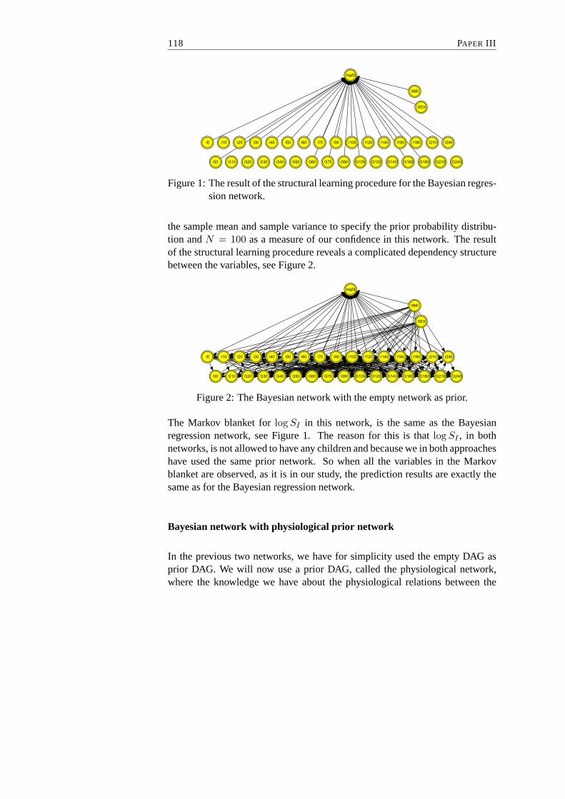
118 PAPER III
Figure 1: The result of the structural learning procedure for the Bayesian regres-sion network.
the sample mean and sample variance to specify the prior probability distribu-tion andN = 100 as a measure of our confidence in this network. The resultof the structural learning procedure reveals a complicateddependency structurebetween the variables, see Figure 2.
Figure 2: The Bayesian network with the empty network as prior.
The Markov blanket forlog SI in this network, is the same as the Bayesianregression network, see Figure 1. The reason for this is thatlog SI , in bothnetworks, is not allowed to have any children and because we in both approacheshave used the same prior network. So when all the variables inthe Markovblanket are observed, as it is in our study, the prediction results are exactly thesame as for the Bayesian regression network.
Bayesian network with physiological prior network
In the previous two networks, we have for simplicity used theempty DAG asprior DAG. We will now use a prior DAG, called the physiological network,where the knowledge we have about the physiological relations between the

PREDICTION OF THEINSULIN SENSITIVITY INDEX 119
variables is incorporated. In this network, insulin measurements and glucosemeasurements are assumed to be Markov processes. They are coupled so thatthe current glucose measurement depends on the previous insulin measurementand the current insulin measurement depends on the current glucose measure-ment, see Figure 3. This structure is consistent with the physiological modelused in Bergmans minimal model to determineSI from an IVGTT. In addition,we let the initial glucose and insulin measurements depend on BMI and sex.
Figure 3: The physiological network.
Like before, we estimate the prior probability distribution from data. However,contrary to the empty network, the variables in the physiological network de-pends on other variables, so we perform a linear regression on the parents anduse the sample mean and sample variance from these regressions as the meanand variance in the local prior probability distributions.Again we useN = 100and we only consider networks where arrows between the glucose and insulinmeasurements point forward in time, where BMI and sex can nothave any par-ents and wherelog SI can not have any children. The result of the structurallearning procedure is shown in Figure 4. As before, we see a complicated de-
Figure 4: The Bayesian network with the physiological network as prior.
pendency structure between the variables. In Figure 5, the Markov blanket oflog SI is shown and we see that is quite different than with the emptyprior,

120 PAPER III
shown in Figure 1. Only 6 of the insulin measurements and 5 of the glucosemeasurements are included in the present blanket.
Figure 5: The Markov blanket for the Bayesian network with the physiologicalnetwork as prior.
Results using multiple linear regression
In Drivsholm et al. (2003), multiple linear regression is used to derive predictiveequations oflog SI using OGTT plasma glucose and serum insulin levels, BMIand gender. To limit the amount of blood samples drawn from the patients, theyconstrain the models to include glucose and insulin observations to the sametime point. By a combination of backwards elimination and forward selection,they find the optimal model to be with sample time points 0, 30,60, 105, 180,and 240. Notice, though, that they have found their model on the basis of adifferent training dataset than ours, as the partition of the dataset into trainingdata and validation data is done randomly in both cases.
Results using the leaps and bound algorithm
Further, we have tried the leaps and bound algorithm by Furnival and Wilson(1974), using the Bayesian information criteria to find the best subset of theexplanatory variables. With this approach, the optimal model is with I50, I90,G160, BMI and sex as explanatory variables. In theory, when the size of thedatabase approaches infinity, using the Bayesian information criteria will resultin the same subset of explanatory variables as when using thenetwork score asselection criteria, see Haughton (1988).

PREDICTION OF THEINSULIN SENSITIVITY INDEX 121
5.3 Evaluation
To compare the different models, we first consider the network score. Noticethat we can only compare network scores for networks that arelearned usingthe same prior network.
To be able to evaluate all models using the network score, we have also cal-culated the log scores for the results found in the multiple linear regressionapproach and the leaps and bounds approach. This is done by formulating theseresults as Bayesian networks and calculating the log scoresusing respectivelythe empty network and the physiological network as prior network. Likewise,for the Bayesian regression network found by using the emptynetwork as priornetwork, we have calculated the log score using the physiological network asprior network.
Model Empty prior Physiological prior
BR −17878.30 −17848.33
BN −16528.39 −14851.44
MLR −17886.17 −17849.06
L&B −17894.95 −17846.12
Table 1: Network scores for the different models.
The results are reported in Table 1. The Bayesian network model (BN) has thelowest log score,i.e. the highest network score, both when the empty networkand the physiological network are used as prior network. This is obvious asthe BN is selected using the network score as selection criteria and because theBayesian regression (BR), the multiple linear regression (MLR) and the leapsand bounds (L&B) networks are included in the search space, when searchingfor the BN with the highest score. So unless we have only founda local max-imum, instead of a global maximum, the score for the BN must behigher thanthe score for the other networks.
When comparing the scores found using the empty prior, we seethat the networkscores for the BR network, the MLR network and the L&B networkare almostall the same. The network score for the BN is over a thousand times higher thanfor any of the other networks, indicating that the BN provides a much better fitto data. Recall, however, that the Markov blanket for the BR network and theBN are the same, so when all the variables in the Markov blanket are observed,the BR network and the BN will predict the samelog SI values. So the highernetwork score is not important when data are complete, but can have an impact

122 PAPER III
when data are incomplete.
When using the physiological network as prior network, we see almost the sameresult. The network score for the BR, MLR and L&B networks arealmost allthe same, whereas the network score for the BN is over 3000 times higher thanfor any of the other networks.
Model Tr. dataR2(SD) Val. dataR2(SD) Tr. outside Val. outside
BR with empty prior 0.76(0.31) 0.73(0.35) 1(1%) 1(2%)
BN with empty prior 0.76(0.31) 0.73(0.35) 1(1%) 1(2%)
BN with physiological prior 0.77(0.30) 0.73(0.36) 7(5%) 3(6%)
MLR 0.76(0.31) 0.66(0.40) 3(2%) 3(6%)
L&B 0.75(0.31) 0.73(0.36) 6(4%) 4(9%)
Table 2: The table lists theR2 andSD values from the linear regressions of theIVGTT obtainedlog SI on the predictedlog SI for both the trainingdataset and the validation dataset. Also listed are how manylog SI
values that fall outside the credibility intervalµ± 1.96 · σ.
In Table 2 theR2 andSD values from the linear regression of the IVGTT ob-tainedlog SI on the predictedlog SI are reported. TheR2 andSD values arefor all five models acceptable and they are almost the same forall models, ex-cept for the multiple regression model, which on the validation dataset does notperform as well as the others. Table 3 shows the intercept andslope of the es-timated regression lines and there are no evidence of any systematic bias. Wetherefore conclude that an OGTT can be used to determine the insulin sensitivityindex.
Model Tr. data (intercept, slope) Val. data (intercept, slope)
BR empty prior (−0.19, 1.09) (−0.05, 1.01)
BN empty prior (−0.03, 1.01) (0.25, 0.87)
BN phsyiological prior (−0.06, 1.03) (0.14, 0.92)
MLR (0, 1) (0.06, 0.96)
L&B (0, 1) (0.11, 0.93)
Table 3: The intercept and slope of the regressions lines from the regressionsof the IVGTT obtainedSI on the predictedSI . Reported to show thatthere is no evidence of systematic bias.
In Table 2 we have also listed how manylog SI values that fall outside thecredibility intervalµ±1.96 ·σ. Approximatively 5% of these predictions should

PREDICTION OF THEINSULIN SENSITIVITY INDEX 123
lie outside and 95% inside the interval for the predictive distributions to be wellcalibrated. This is clearly fulfilled for the BN with the physiological networkas prior network, so the predictive distribution forlog SI is, when using thisnetwork, well calibrated. With the MLR approach and the L&B approach itis almost fulfilled that 5% of the predictions lie outside the intervals. We willtherefore conclude that the predictive distributions are also well calibrated inthese cases. For the BR and the BN with the empty network as prior network,very few values lie outside the intervals, indicating that the variance is probablyestimated to large. Figure 6 shows the predictedlog SI values and the intervalsfor the BN with the empty prior and for the BN with the physiological prior. Wesee that for the two models, the predictedlog SI values are almost the same, butthe intervals are much wider for the BN with the empty prior, meaning that thevariance in this model is larger.
0 10 20 30 40
−2
−1
01
2
Case
Est
. log
(SI)
− T
rue
log(
SI)
Figure 6: The predictedlog SI values and the credibility intervals for theBayesian network with empty prior (dark and disks) versus theBayesian network with physiological prior (light and triangles).
So to summarize, all the models give adequate predictions ofthe log SI values.Evaluating the models using the different validation approaches all together, theBN with the physiological prior model gives a more precise predictive distri-bution of log SI compared to the other models. We therefore suggest that thismodel should be used to derive the predictive values oflog SI .

124 PAPER III
6 Discussion
We have established a promising way of determining the insulin sensitivity in-dex from an oral glucose tolerance test rather than from an intravenous glucosetolerance test. All approaches give adequate predictions of SI . The Bayesiannetwork with the physiological prior estimates the most precise predictive distri-bution ofSI , so we claim that this is the best model. There are also other advan-tages by using a Bayesian network instead of an ordinary regression model. In aBayesian network, we can use any prior knowledge available frome.g.previousstudies or from the physiological understanding of the problem. Further, we cancalculate the predictive distribution oflog SI in situations, where some of theobservations are missing. This can be used when a single or a few observationsare missing for a specific subject. It can also be used when certain time pointsare not observed at all, which could be the case if a dataset from another study,using fewer time points, is analyzed.
Acknowledgements
This work has been supported by Novo Nordisk A/S. The collection of datawere done by Torben Hansen, Novo Nordisk A/S.
References
Bergman, R. N., Ider, Y. Z., Bowden, C. R. and Cobelli, C. (1979). Quan-titative estimation of insulin sensitivity,American Journal of Physiology236: E667–E677.
Bøttcher, S. G. (2001). Learning Bayesian Networks with Mixed Variables,Ar-tificial Intelligence and Statistics 2001, Morgan Kaufmann, San Francisco,CA, USA, pp. 149–156.
Bøttcher, S. G. and Dethlefsen, C. (2003).deal: A Package for LearningBayesian Networks,Journal of Statistical Software8(20): 1–40.
Cooper, G. and Herskovits, E. (1992). A Bayesian method for the induction ofprobabilistic networks from data,Machine Learning9: 309–347.

PREDICTION OF THEINSULIN SENSITIVITY INDEX 125
Cowell, R. G., Dawid, A. P., Lauritzen, S. L. and Spiegelhalter, D. J. (1999).Probabilistic Networks and Expert Systems, Springer-Verlag, Berlin-Heidelberg-New York.
Dawid, A. P. (1982). The Well-Calibrated Bayesian,Journal of the AmericanStatistical Association77(379): 605–610.
Drivsholm, T., Hansen, T., Urhammer, S. A., Palacios, R. T.,Vølund, A., Borch-Johnsen, K. and Pedersen, O. B. (2003). Assessment of insulin sensitivityindex and acute insulin reponse from an oral glucose tolerance test in sub-jects with normal glucose tolerance, Novo Nordisk A/S.
Furnival, G. M. and Wilson, R. W. (1974). Regression by Leapsand Bounds,Technometrics16(4): 499–511.
Geiger, D. and Heckerman, D. (1994). Learning Gaussian Networks,Proceed-ings of Tenth Conference on Uncertainty in Artificial Intelligence, MorganKaufmann, San Francisco, CA, USA, pp. 235–243.
Haughton, D. M. A. (1988). On The Choice of a Model to fit Data From anExponential Family,The Annals of Statistics16(1): 342–355.
Heckerman, D., Geiger, D. and Chickering, D. M. (1995). Learning Bayesiannetworks: The combination of knowledge and statistical data, MachineLearning20: 197–243.
Ihaka, R. and Gentleman, R. (1996). R: A language for data analysis and graph-ics,Journal of Computational and Graphical Statistics5: 299–314.
Lauritzen, S. L. (1992). Propagation of probabilities, means and variances inmixed graphical association models,Journal of the American StatisticalAssociation87(420): 1098–1108.
Martin, B. C., Warram, J. H., Krolewski, A. S., Bergman, R. N., Soeldner, J. S.and Kahn, C. R. (1992). Role of glucose and insulin resistance in develop-ment of type 2 diabetes mellitus: results of a 25-year follow-up study,TheLancet340: 925–929.
Pacini, G. and Bergman, R. N. (1986). MINMOD: a computer program to cal-culate insulin sensitivity and pancreatic responsivity from the frequentlysampled intraveneous glucose tolerance test,Computer Methods and Pro-grams in Biomedicine23: 113–122.

126 PAPER III

Paper IVLearning Dynamic Bayesian Networks
with Mixed Variables
Susanne G. Bøttcher
127


Learning Dynamic Bayesian Networkswith Mixed Variables
Susanne G. Bøttcher
Aalborg University, Denmark
Abstract.This paper considers dynamic Bayesian networks for discrete and continuous vari-ables. We only treat the case, where the distribution of the variables is conditionalGaussian. We show how to learn the parameters and structure of a dynamicBayesian network and also how the Markov order can be learned. An auto-mated procedure for specifying prior distributions for the parameters in a dynamicBayesian network is presented. It is a simple extension of the procedure for theordinary Bayesian networks. Finally the Wölfer’s sunspot numbers are analyzed.
1 Introduction
In this paper we consider dynamic Bayesian networks (DBNs) for discrete andcontinuous variables. A DBN is an extension of an ordinary Bayesian networkand is applied in the modeling of time series.
DBNs for first order Markov time series are described in Dean and Kanazawa(1989). In Murphy (2002), a thorough treatment of these models is presentedand in Friedman et al. (1998) learning these networks in the case with onlydiscrete variables is described.
Here we consider DBNs with both discrete and continuous variables. In thesenetworks we also allow some of the variables to be static,i.e. some of the vari-ables do not change over time. We only treat the case where thedistribution ofthe variables is conditional Gaussian (CG) and show how to learn the parametersand structure of the DBN when data is complete. Further we present an auto-mated method for specifying prior parameter distributionsfor the parametersin a DBN. These methods are simple extensions of the ones usedfor ordinaryBayesian networks with mixed variables, described in Bøttcher (2001).
We consider time series, where the Markov order can be higherthan one andshow how the Markov order can be learned.
In Section 2, DBNs with static and time varying variables aredefined. Section 3
129

130 PAPER IV
presents these DBNs for the mixed case and Section 4 gives some examples ofsome well known models that can be represented as DBNs. Section 5 shows howto learn the parameters and structure of a DBN with mixed variables. Further,it shows how the Markov order can be learned. Section 6 presents a methodfor specifying prior distributions of the parameters in theDBN. In Section 7Wölfer’s sunspot numbers are analyzed using a DBN.
2 Dynamic Bayesian Networks
A Bayesian networkis a graphical model that encodes the joint probabilitydistribution for a set of variables. For terminology and theoretical aspects ongraphical models, see Lauritzen (1996). We define it as adirected acyclic graph(DAG) D = (V, E), whereV is a finite set of nodes andE is a finite set of di-rected edges between the nodes. The DAG defines the structureof the Bayesiannetwork. To each nodev ∈ V in the graph corresponds a random variableXv.The set of variables associated with the graphD is thenX = (Xv)v∈V .
To each vertexv with parents pa(v), there is attached a local probability distribu-tion,p(xv|xpa(v)). The possible lack of directed edges inD encodes conditionalindependencies between the random variablesX through the factorization ofthe joint probability distribution,
p(x) =∏
v∈V
p(xv|xpa(v)).
In a Bayesian network, the set of random variablesX is fixed. To model amultivariate time series we need a framework, where we allowthe set of randomvariables to vary with time. For this we use dynamic Bayesiannetworks, definedas below. This definition is consistent with the exposition in Murphy (2002), buthere we also allow for static variables and Markov orders higher than one.
Let Xt be a set of time varying random variables, that isXt can take on the val-uesX0, X1, . . . , XT . We index the time varying variables by the non-negativeintegers to indicate that the observations are taken at discrete time points. Thecorresponding nodes in the graph are denotedVt, soXt = (Xt
v)v∈Vt for eachtime pointt. Note however thatVt is “the same” for all time pointst, so for-mally Vt = {(v, t), v ∈ V }. Further, letXs be a set of static random vari-ables,i.e. variables that do not change over time. The nodes corresponding

LEARNING DYNAMIC BAYESIAN NETWORKS WITH M IXED VARIABLES 131
to Xs are denotedVs. The set of variables associated with a DBN is thenX = ((Xt)T
t=0, Xs) and the set of nodes isV = ((Vt)
Tt=0, Vs).
We refer to the time varying variables at one time point as atime sliceor justa slice. We let the static variablesXs belong to the time slice at timet = 0and refer to this as the initial time slice. So the initial time slice includes thevariablesX0 andXs and, fort = 1, . . . , T , the time slice at timet includes thevariablesXt.
We will mostly consider the variables in the initial time slice jointly, so to easelater notation we defineX 0 = (X0, Xs) andV0 = (V0, Vs).
The joint probability distribution of the variables in a dynamic Bayesian networkcan be very complex, as the number of variables grows over time. Therefore weassume that the time series we are dealing with, ismth order Markov, i.e.
p(xt|xt−1, . . . , x0) = p(xt|xt−1, . . . , xt−m),
for all time pointst = m, . . . , T .
Further, we assume that the time series hasstationary dynamics, so
p(xt|xt−1, . . . , xt−m) = p(xm|xm−1, . . . , x0),
for all t = m, . . . , T . Stationary dynamics refers to the fact that the conditionaldistributions are time independent, while the marginal distributions may be timedependent.
We will first introduce DBNs for time series that are first order Markov. With theabove assumptions, a DBN for a first order Markov time series can be defined tobe the pair(B0, B→), whereB0 is a Bayesian network defining the probabilitydistribution ofX 0 as
p(x0) =∏
v∈V0
p(x0v|x
0
pa(v)),
andB→ is a2-slice temporal Bayesian network defining the conditional distri-bution ofXt as
p(xt|xt−1, xs) =∏
v∈Vt
p(xtv|x
tpa(v), x
t−1pa(v), x
spa(v)).
The joint probability distribution for a DBN withT + 1 time points is given as
p(x0, . . . , xT , xs) = p(x0)
T∏
t=1
p(xt|xt−1, xs).

132 PAPER IV
As we assumed that the time series has stationary dynamics, the DBN is com-pletely specified throughB0 andB→.
For the dependency relations between the time slices we assume that arrowspoint forward in time, so the variables in time slicet can have parents in thetime slices to timet andt− 1. Further, they can have parents fromXs. Due tostationary dynamics, the dependency relations between thetime slices are thesame for all time points. This also means that if a time varying variableXt
v hasa static variableXs
w as a parent, thenXsw is also a parent ofX1
v, . . . , XTv . The
variables in the initial time slice can have parents from theinitial time slice andtherefore also fromXs, asXs is included in the initial time slice.
Within a time slice, there are no restrictions of the dependency relations betweenthe variables, as long as the structure is a DAG. Due to stationary dynamics, thedependency relations within a time slice are the same for thetime slices to timet = 1, . . . , T . They are however not necessarily the same as for the time varyingvariables in the initial time slice.
So the structure of the DBN repeats itself over time, except for B0, where thetime series is initialized.
Figure 1 shows an example of the structure of a a first order Markov DBN,(B0, B→), with two time varying variablesY t andZt and one static variableXs. Because of the first order Markov property, the structure iscompletelyspecified through the first two time points and the structure of the DBN cantherefore be represented by the DAG in Figure 2.
Xs
Z0
Y 0
Xs
Zt−1 Zt
Y t−1 Y t
B0 B→
Figure 1: Example of a first order Markov DBN(B0, B→).
For time series with higher Markov order properties, we needto extend thedefinition.
Consider anmth order Markov time series. The joint probability distribution

LEARNING DYNAMIC BAYESIAN NETWORKS WITH M IXED VARIABLES 133
Xs
Z0 Z1
Y 0 Y 1
Figure 2: A first order Markov DBN(B0, B→) represented by the first two timepoints.
for T + 1 time points can be written as
p(x0, . . . , xT , xs) = p(x0, x1, . . . , xm−1)T∏
t=m
p(xt|xt−1, . . . , xt−m, xs)
= p(x0)p(x1|x0) · · · , p(xm−1|xm−2, . . . , x0)
×T∏
t=m
p(xt|xt−1, . . . , xt−m, xs).
Following the definition for first order Markov time series, we let B→ be am + 1-slice temporal Bayesian network defining the conditional distribution ofXt,
p(xt|xt−1, . . . , xt−m, xs) =∏
v∈Vt
p(xtv|x
tpa(v), . . . , x
t−mpa(v), x
spa(v)),
for t = m, . . . , T .
The variables in time slicet can have parents in the time slices to timest, . . . , t−m and they can have parents fromXs. Again, due to stationary dynamics, thedependency relations between and within the time slices arethe same for alltime pointst = m, . . . , T . Further, if a time varying variableXt
v has a staticvariableXs
w as a parent, thenXsw is also a parent ofXm
v , . . . , XTv .
The question is now how to initialize the time series. The probability distribu-tion p(x0, x1, . . . , xm−1) can be written as
p(x0, x1, . . . , xm−1) = p(x0)p(x1|x0) · · · p(xm−1|xm−2, . . . , x0). (1)
As arrows point forward in time, this factorization defines the possible depen-dency relations between the variablesX 0, . . . , Xm−1. As before we letB0 be a

134 PAPER IV
Bayesian network defining the probability distribution ofX 0 as
p(x0) =∏
v∈V0
p(x0v|x
0
pa(v)).
Now we also define Bayesian networks for the rest of the conditional distribu-tions in (1). We letB1 be a2-slice Bayesian network defining the conditionaldistribution ofX1 givenX 0 as
p(x1|x0) =∏
v∈V1
p(x1v|x
1pa(v), x
0
pa(v)),
and likewise forB2, . . . , Bm−1, whereBm−1 is anm-slice Bayesian networkdefining the conditional distribution ofXm−1 givenXm−2, . . . , X 0 as
p(xm−1|xm−2, . . . , x0) =∏
v∈Vm−1
p(xm−1v |xm−1
pa(v), . . . , x0
pa(v)).
So the variables in the time slice to timet = 1 can have parents from the timeslice to timet = 1 and t = 0. The variables in time slicem − 1 can haveparents from the time slices to timet = 0, . . . , m−1. The dependency relationsbetween the time slices to timet = 0, . . . , m−1 are obviously not the same andthe dependency relations within these time slices are not necessarily the same.
The tuple(B0, B1, . . . , Bm−1, B→) is thus a DBN for anmth order Markovtime series, where the different Bayesian networks in the tuple defines the cor-responding probability distributions as above. Notice that we could also justhave specified the networksB0, B1, . . . , Bm−1 as one large network, with thenecessary restrictions on the arrows.
3 Dynamic Bayesian Networks for Mixed Variables
In this section we consider DBNs withmixed variables, i.e. the variables in thenetwork can be of discrete and continuous type. We letV = ∆ ∪ Γ, where∆andΓ are the sets of discrete and continuous variables, respectively. The corre-sponding random variablesX can then be denotedX = (Xv)v∈V = (I, Y ) =((Iδ)δ∈∆, (Yγ)γ∈Γ). Again, we index the sets of nodes and the random variableswith t for time varying variables,s for static variables and0 for the variables inthe initial time slice.

LEARNING DYNAMIC BAYESIAN NETWORKS WITH M IXED VARIABLES 135
To ensure availability of exact local computation methods,we do not allow con-tinuous parents of discrete nodes, so the probability distributions factorize intoa discrete part and a mixed part as presented below. To simplify notation, wepresent the theory for first order Markov time series and comment on how toextend it to higher order Markov assumptions by following the definitions intro-duced in the previous section.
We considerB0 andB→ separately, and the joint probability distribution is ob-tained as specified in the previous section.
ForB0 we have that
p(x0) =∏
v∈V0
p(x0v|x
0
pa(v))
=∏
δ∈∆0
p(i0δ|i0
pa(δ))∏
γ∈Γ0
p(y0γ |i
0
pa(γ), y0
pa(γ)) (2)
and forB→
p(xt|xt−1, xs) =∏
v∈Vt
p(xtv|x
tpa(v), x
t−1pa(v), x
spa(v))
=∏
δ∈∆t
p(itδ|itpa(δ), i
t−1pa(δ), i
spa(δ)) (3)
×∏
γ∈Γt
p(ytγ |i
tpa(γ), i
t−1pa(γ), i
spa(γ), y
tpa(γ), y
t−1pa(γ), y
spa(γ)).
To account for higher order Markov assumptions, we would just have to specifythe probability distributions for the intervening networks accordingly.
To simplify notation forB→, we use the following notation, where the possibleparent configurations are not explicitly defined. They must be specified in thegiven context and according to (3).
p(xt|xt−1, xs) =∏
v∈Vt
p(xtv|x
→pa(v))
=∏
δ∈∆t
p(itδ|i→pa(δ))
∏
γ∈Γt
p(ytγ |i
→pa(γ), y
→pa(γ)).
So for example,i→pa(δ) contains the variablesitpa(δ), it−1pa(δ) andispa(δ).
In this paper we only consider networks, where the joint distribution of the vari-ables is conditional Gaussian. The local probability distributions are therefore

136 PAPER IV
defined as in the following two sections. In these sections, we do not distinguishbetween the variables inB0 andB→, as the distribution of these variables is ofthe same type. The possible parent set differ however between variables inB0
and variables inB→. In the following we therefore just denote the parents of avariablexv by xpa(v) andxpa(v) must be specified according to (2) or (3).
3.1 Distribution for Discrete Variables
When the joint distribution is conditional Gaussian, the local probability distri-butions for the discrete variables are just unrestricted discrete distributions with
p(iδ|ipa(δ)) ≥ 0 ∀ δ ∈ ∆.
We parameterize this as
θiδ |ipa(δ)= p(iδ|ipa(δ), θδ|ipa(δ)
),
whereθδ|ipa(δ)= (θiδ|ipa(δ)
)iδ∈Iδ.
Furthermore∑
iδ∈Iδθiδ |ipa(δ)
= 1 and0 ≤ θiδ|ipa(δ)≤ 1. All parameters associ-
ated with a nodeδ is denoted byθδ, soθδ = (θδ|ipa(δ))ipa(δ)∈Ipa(δ)
.
3.2 Distribution for Continuous Variables
For the continuous variables, the local probability distributions are Gaussian lin-ear regressions with parameters depending on the configuration of the discreteparents. So let the parameters be given byθγ|ipa(γ)
= (mγ|ipa(γ), βγ|ipa(γ)
, σ2γ|ipa(γ)
).
Then
(Yγ |ypa(γ), ipa(γ), θγ|ipa(γ)) ∼ N (mγ|ipa(γ)
+ βγ|ipa(γ)ypa(γ) , σ2
γ|ipa(γ)), (4)
whereβγ|ipa(γ)are the regression coefficients,mγ|ipa(γ)
is the regression inter-
cept, andσ2γ|ipa(γ)
is the conditional variance. Thus for each configuration of
the discrete parents ofγ the distribution ofYγ is Gaussian with mean andvariance given as in (4). The parameters associated with a node γ is thenθγ = (θγ|ipa(γ)
)ipa(γ)∈Ipa(γ).

LEARNING DYNAMIC BAYESIAN NETWORKS WITH M IXED VARIABLES 137
3.3 The Parameterized Distributions
With the above distributional assumptions, we can specify the parameterizedDBN as follows.
Let θ0 = ((θ0δ)δ∈∆0
, (θ0γ)γ∈Γ0
) andθ→ = ((θ→δ )δ∈∆t, (θ→γ )γ∈Γt). Further, let
θ = (θ0, θ→). ThenB0 is given as
p(x0|θ0) =∏
δ∈∆0
p(i0δ|i0
pa(δ), θ0
δ|ipa(δ))∏
γ∈Γ0
p(y0γ |i
0
pa(γ), y0
pa(γ), θ0
γ|ipa(γ)),
andB→ as
p(xt|xt−1, xs, θ→) =∏
δ∈∆t
p(itδ|i→pa(δ), θ
→δ|ipa(δ)
)
×∏
γ∈Γt
p(ytγ |y
→pa(γ), i
→pa(γ), θ
→γ|ipa(γ)
).
The joint distribution forT + 1 time points is given as
p(x0, . . . , xT , xs, θ) = p(x0|θ0)
T∏
t=1
p(xt|xt−1, xs, θ→).
Notice that, due to stationarity,θ→ is the parameter in the conditional distribu-tion of xt for everytime pointt = 1, . . . , T .
4 Examples of DBNs
We will now give some examples of some well known models that can be rep-resented as DBNs. In the figures, shaded nodes represent discrete variables andclear nodes represent continuous variables.
4.1 Hidden Markov Models
A Hidden Markov Model (HMM) is a stochastic automaton, whereeach stategenerates an observation. Figure 3 shows a HMM, where the hidden states are

138 PAPER IV
first order Markov.
I0
I1
I2
I3 · · ·
Y0
Y1
Y2
Y3 · · ·
Figure 3: A Hidden Markov Model.
The hidden states,i.e. the discrete hidden variables, are denoted byI and theobservations byY . We have represented the observed variables as continuous,but they can also all be discrete. In this HMM,It+1 is conditionally indepen-dent ofIt−1, givenIt. Further,Y t is conditionally independent of the rest ofthe variables in the network, givenIt. A model like this is used in situations,where the observations do not follow the same model all the time, but can fol-low different models at different times. This gives for example the possibility toaccount for outliers.
When a HMM is represented as a DBN, we assume that the time series hasstationary dynamics. So, together with the first order Markov property, we canspecify the joint probability distribution for the variables in this network byjust specifying the initial prior probabilitiesp(i0), the transition probabilitiesp(it|it−1) and the conditional Gaussian distributionsp(yt|it) (or, if the observedvariables are discrete, the conditional multinomial distributionsp(jt|it)).
There are many variants of this basic HMM,e.g.Buried Markov Model, Mixed-memory Markov Model and Hierarchical HMM, see Murphy (2002)for a pre-sentation of these models represented as DBNs and their application withinspeech recognition.
4.2 Kalman Filter Models
A Kalman Filter Model (KFM), introduced by Harrison and Stevens (1976) asa state space model, models the dynamic behavior of a time series. In sucha model, the continuous observationsY are indirect measurements of a latentMarkov processZ.
In Figure 4, a KFM is shown. The structure is the same as for theHMM, sincethe two models assume the same set of conditional independencies. The proba-bility distributions to be specified is the Gaussian distribution p(z0), the Gaus-

LEARNING DYNAMIC BAYESIAN NETWORKS WITH M IXED VARIABLES 139
Z0
Z1
Z2
Z3 · · ·
Y0
Y1
Y2
Y3 · · ·
Figure 4: A Kalman Filter Model.
sian linear regressionp(zt|zt−1) and the Gaussian linear regressionp(yt|zt).For a comprehensive treatment of KFMs and their applications, see West andHarrison (1989).
4.3 Multiprocess Kalman Filter Models
Multiprocess Kalman Filter Models (MKFMs), also known as switching statespace Markov models, are an extension of the KFMs, see Harrison and Stevens(1976), where the aim is to discriminate between different KFMs.
I0
I1
I2
I3 · · ·
Z0
Z1
Z2
Z3 · · ·
Y0
Y1
Y2
Y3 · · ·
Figure 5: A Multiprocess Kalman Filter Model.
Figure 5 shows a MKFM. Again we see that the continuous observationsY areindirect measurements of a latent continuous Markov process Z, i.e. this partof the network represents a KFM. In addition, the processZ depends on thehidden statesI, which in our example are first order Markov. Like the HMM,this model can be used in situations, where the observationsdo not follow thesame model all the time, but can follow different models at different times, buthere the models are KFMs. Applications include modeling piece-wise lineartime series, which for example can be used for monitoring purposes, seee.g.Bøttcher, Milsgaard and Mortensen (1995).
Notice that because of the first order Markov property assumed for HMMs,KFMs and MKFMs, these models could have been represented by using onlythe first two time points, as the structure repeats over time.

140 PAPER IV
4.4 Vector Autoregressive processes
Another classical time series model is the Vector Autoregressive process (VAR)of Markov orderp. This model is equivalent to a DBN of Markov orderp, inwhich all the variables are continuous and observed. So the local probabilitydistributions in this model are Gaussian linear regressions on the continuousparents.
t = 0 t = 1 t = 2
· · ·
· · ·
· · ·
· · ·
Figure 6: A Vector Autoregressive process.
In Figure 6, an example of a VAR process of order2 is given. Because of thesecond order Markov property, this model can be representedby the first threetime points.
In the next section, we will developed a method for learning the parameters andstructure of a DBN. In this paper we assume that data are complete, so we cannot learn networks with hidden variables. Therefore, the HMM, the KFM andthe MKFM can only be learned with these methods, if a trainingdataset withcomplete data is available.
5 Learning DBNs with Mixed Variables
Learning first order Markov DBNs in the purely discrete case with no staticvariables is described in Friedman et al. (1998). Here we will consider learningDBNs with mixed variables for the case with both time varyingand static vari-ables. Further, we will also illustrate how to learn DBNs with higher Markovorder and how to learn this order.
As noted in Murphy (2002), learning DBNs is, because of the way DBNs aredefined, just a simple extension of learning BNs. This also applies for DBNs
LEARNING DYNAMIC BAYESIAN NETWORKS WITH M IXED VARIABLES 141
with mixed variables, so we will use the theory for learning Bayesian networkswith mixed variables, described in Bøttcher (2001).
5.1 Parameter Learning
To learn the parameters for a given DAG, we use a Bayesian approach. We spec-ify a prior distribution of a parameterθ, use a random sampled from the prob-ability distributionp(x|θ) and obtain the posterior distribution by using Bayes’theorem
p(θ|d) ∝ p(d|θ)p(θ).
The proportionality constant is determined by the relation∫
Θ p(θ|d)dθ = 1,whereΘ is the parameter space.
To obtain closed formed expressions, we use conjugate distributions of the pa-rameters.
We assume that the parameters associated withB0 andB→ are independent.Further, for the parameters in respectivelyB0 andB→, we assume that the pa-rameters associated with one variable is independent of theparameters associ-ated with the other variables and that the parameters are independent for eachconfiguration of the discrete parents,i.e.
p(θ) = p(θ0)p(θ→)
=∏
δ∈∆0
∏
ipa(δ)∈Ipa(δ)
p(θ0
δ|ipa(δ))∏
γ∈Γ0
∏
ipa(γ)∈Ipa(γ)
p(θ0
γ|ipa(γ)) (5)
×∏
δ∈∆t
∏
ipa(δ)∈Ipa(δ)
p(θ→δ|ipa(δ))∏
γ∈Γt
∏
ipa(γ)∈Ipa(γ)
p(θ→γ|ipa(γ)).
We refer to this asparameter independence. Notice though that it is slightlydifferent than parameter independence for ordinary Bayesian networks, as wehere assume that the parameters inB→ are the same for each time pointt =1, . . . , T .
In the case with higher order Markov properties, parameter independence is alsovalid for the parameters in the networksB1, . . . , Bm−1.
We also assumecomplete data, i.e. each casecx in a datasetd contains one in-stance of every random variable in the network. With this we can show posteriorparameter independence. The likelihoodp(d|θ) can be written as follows.

142 PAPER IV
p(d|θ) =∏
c∈d
p(cx0, . . . , cxT , cxs|θ)
=∏
c∈d
(
p(cx0|θ0)T∏
t=1
p(cxt|cxt−1, cxs, θ→)
)
.
As the time series has stationary dynamics, we see that for each observations ofthe variables inB0, there areT observations of the variables inB→.
To simplify the expressions, we consider the likelihood terms forB0 andB→
separately. ForB0 we have that
∏
c∈d
p(cx0|θ0) =∏
c∈d
∏
δ∈∆0
p(ci0δ|ci0pa(δ), θ
0
δ|ipa(δ))∏
γ∈Γ0
p(cy0γ |
cy0
pa(γ),ci0pa(γ), θ
0
γ|ipa(γ)),
whereci andcy respectively denotes the discrete part and the continuous part of acasecx. Our goal is to show posterior parameter independence, so wemust showthat the likelihood, like the parameters, factorizes into aproduct over nodes anda product over the configuration of the discrete parents of a node. Therefore wewrite this part of the likelihood as
∏
c∈d
p(cx0|θ0) =∏
δ∈∆
∏
ipa(δ)∈Ipa(δ)
∏
c:ci0pa(δ)=i0pa(δ)
p(ci0δ|i0
pa(δ), θ0
δ|ipa(δ))
×∏
γ∈Γ
∏
ipa(γ)∈Ipa(γ)
∏
c:ci0pa(γ)=i0pa(γ)
p(cy0γ |
cy0
pa(γ), i0
pa(γ), θ0
γ|ipa(γ)).
(6)
We see that the product over cases is split up into a product over the configura-tions of the discrete parents and a product over those cases,where the configura-tion of the discrete parents is the same as the currently processed configuration.Notice however that some of the parent configurations might not be representedin the database, in which case the product over cases with this parent configura-tion just adds nothing to the overall product.
In the case withmth order Markov properties, the likelihood terms for all thenetworksB1, . . . , Bm−1, can be written as in (6).

LEARNING DYNAMIC BAYESIAN NETWORKS WITH M IXED VARIABLES 143
The likelihood part fromB→ is given as,
∏
c∈d
T∏
t=1
p(cxt|cxt−1, cxs, θ→)
=∏
c∈d
T∏
t=1
∏
δ∈∆t
p(citδ|ci→pa(δ), θ
→δ|ipa(δ)
)∏
γ∈Γt
p(cytγ |
cy→pa(γ),ci→pa(γ), θ
→γ|ipa(γ)
)
=∏
δ∈∆t
∏
i→pa(δ)∈I→pa(δ)
T∏
t=1
∏
c:ci→pa(δ)=i→pa(δ)
p(citδ|i→pa(δ), θ
→δ|ipa(δ)
) (7)
×∏
γ∈Γ
∏
i→pa(γ)∈I→
pa(γ)
T∏
t=1
∏
c:ci→pa(γ)=i→pa(γ)
p(cytγ |
cy→pa(γ), i→pa(γ), θ
→γ|ipa(γ)
)
The product over cases is split up as before. Further, this isalso a product overtime points, so for each time pointt, we take the product over cases with aspecific configuration of the discrete parents.
Posterior parameter independence now follows from (5), (6)and (7),
p(θ|d) = p(θ0|d)p(θ→|d)
=∏
δ∈∆0
∏
ipa(δ)∈Ipa(δ)
p(θ0
δ|ipa(δ)|d)
∏
γ∈Γ0
∏
ipa(γ)∈Ipa(γ)
p(θ0
γ|ipa(γ)|d)
×∏
δ∈∆t
∏
ipa(δ)∈Ipa(δ)
p(θ→δ|ipa(δ)|d)
∏
γ∈Γt
∏
ipa(γ)∈Ipa(γ)
p(θ→γ|ipa(γ)|d).
So due to parameter independence and complete data, the parameters stay in-dependent given data. This means that we can learn the parameters in the localdistributions independently and also that the parameters in B0 andB→ can belearned independently. Again, if the time series ismth order Markov, poste-rior parameter independence also follows and we can learn the parameters inB0, . . . , Bm−1 andB→ independently.
Consider for example inB0 a parameter for a discrete nodeδ, with a specificconfiguration of the discrete parents,ipa(δ). The posterior distribution ofθ0
δ|ipa(δ)

144 PAPER IV
is by Bayes’ theorem found as
p(θ0
δ|ipa(δ)|d) ∝
∏
c:ci0pa(δ)=i0pa(δ)
p(ci0δ|i0
pa(δ), θ0
δ|ipa(δ))p(θ0
δ|ipa(δ)).
Thusθ0
δ|ipa(δ)is updated with the cases in the database, where the configuration
of the parents ofδ is i0pa(δ).
Likewise with a parameterθ→δ|ipa(δ)in B→,
p(θ→δ|ipa(δ)|d) ∝
T∏
t=1
∏
c:ci→pa(δ)=i→pa(δ)
p(citδ|i→pa(δ), θ
→δ|ipa(δ)
)p(θ→δ|ipa(δ)).
Hereθ→δ|ipa(δ)is, for each time pointt, updated with the cases in the database for
which the configuration of the parents ofδ is i→pa(δ).
In the next sections we will introduce the conjugate distributions of the parame-ters and show how these are learned. The only difference in how the parametersin B0 andB→ are learned, is the set of cases used to learn them. So in thefollowing we do not differentiate between the parameters inB0 andB→.
5.2 Learning the Discrete Variables
As described in DeGroot (1970), a conjugate family for multinomial observa-tions is the family of Dirichlet distributions. Let the prior distribution ofθδ|ipa(δ)
be a Dirichlet distribution,D, with hyperparametersαδ|ipa(δ)= (αiδ|ipa(δ)
)iδ∈Iδ,
also written as(θδ|ipa(δ)
|αδ|ipa(δ)) ∼ D(αδ|ipa(δ)
).
The posterior distribution is then given as
(θδ|ipa(δ)|d) ∼ D(αδ|ipa(δ)
+ nδ|ipa(δ)),
where the vectornδ|ipa(δ)= (niδ|ipa(δ)
)iδ∈Iδ, also called the counts, denotes the
number of observations ind whereδ and pa(δ) have that specific configuration.
Again αδ|ipa(δ)andnδ|ipa(δ)
can be indexed by0 and→, according toB0 and
B→. So forB0 we have thatn0
iδ|ipa(δ)is the number of cases ind with a given
configuration ofδ and pa(δ). Likewise forB→, wheren→iδ|ipa(δ)
is the number
of cases ind and for every time pointt = 1, . . . , T , with this configuration ofδand pa(δ).

LEARNING DYNAMIC BAYESIAN NETWORKS WITH M IXED VARIABLES 145
5.3 Learning the Continuous Variables
For the continuous variables we can write the local probability distributions as
(Yγ |ypa(γ), ipa(γ), θγ|ipa(γ)) ∼ N (zpa(γ)(mγ|ipa(γ)
, βγ|ipa(γ))T, σ2
γ|ipa(γ)),
wherezpa(γ) = (1, ypa(γ)). A standard conjugate family for these observationsis the family of Gaussian-inverse gamma distributions. Letthe prior joint distri-bution of(mγ|ipa(γ)
, βγ|ipa(γ)) andσ2
γ|ipa(γ)be as follows.
(mγ|ipa(γ), βγ|ipa(γ)
|σ2γ|ipa(γ)
) ∼ Nk+1(µγ|ipa(γ), σ2
γ|ipa(γ)τ−1γ|ipa(γ)
),
(σ2γ|ipa(γ)
) ∼ IΓ
(
ργ|ipa(γ)
2,φγ|ipa(γ)
2
)
.
If θγ|ipa(γ)is a parameter inB0, the posterior distribution is found by
p(θ0
γ|ipa(γ)|d) ∝
∏
c:ci0pa(γ)=i0pa(γ)
p(cy0γ |
cy0
pa(γ), i0
pa(γ), θ0
γ|ipa(γ))p(θ0
γ|ipa(γ)).
We now join all the observationscy0γ for which ci0
pa(γ) = i0pa(γ) in a vectorby0
γ , i.e.by0
γ = (cy0γ)ci0pa(γ)
=i0pa(γ)
.
The same is done with the observations of the continuous parents of γ, i.e.by0
pa(γ) = (cy0
pa(γ))ci0pa(γ)=i0pa(γ)
. The posterior distribution ofθγ|ipa(γ)can now
be written as
p(θ0
γ|ipa(γ)|d) ∝ p(by0
γ |by0
pa(γ), i0
pa(γ), θ0
γ|ipa(γ))p(θ0
γ|ipa(γ)).
As the distribution,p(cy0γ |
cy0
pa(γ), i0
pa(γ), θ0
γ|ipa(γ)), is a Gaussian distribution, then
p(by0γ |
by0
pa(γ), i0
pa(γ), θ0
γ|ipa(γ)) is a multivariate Gaussian distribution. The covari-
ance matrix is diagonal as all the cases in the database are independent. Thisway we consider all the cases in abatch.
The same formulation applies for parameters inB→. Notice that the observa-tions included inby→γ andby→pa(γ) are taken for each time pointt = 1, . . . , T .

146 PAPER IV
The posterior distribution is found to be
(mγ|ipa(γ), βγ|ipa(γ)
|σ2γ|ipa(γ)
, d) ∼ Nk+1(µ′γ|ipa(γ)
, σ2γ|ipa(γ)
(τ−1γ|ipa(γ)
)′)
(σ2γ|ipa(γ)
|d) ∼ IΓ
(
ρ′γ|ipa(γ)
2,φ′
γ|ipa(γ)
2
)
,
where
τ ′γ|ipa(γ)
= τγ|ipa(γ)+ (zb
pa(γ))Tzb
pa(γ)
µ′γ|ipa(γ)
= (τ ′γ|ipa(γ)
)−1(τγ|ipa(γ)µγ|ipa(γ)
+ (zbpa(γ))
Tybγ)
ρ′γ|ipa(γ)= ργ|ipa(γ)
+ |b|
φ′γ|ipa(γ)
= φγ|ipa(γ)+ (yb
γ − zbpa(γ)µ
′γ|ipa(γ)
)Tybγ
+(µγ|ipa(γ)− µ′
γ|ipa(γ))Tτγ|ipa(γ)
µγ|ipa(γ),
where|b| denotes the number of observations inybγ .
5.4 Structure Learning
To learn the structure of a DBN, we again use a Bayesian approach and calculatethe posterior probability of a DAGD given datad,
p(D|d) ∝ p(d|D)p(D), (8)
wherep(d|D) is the marginal likelihood ofD andp(D) is the prior probabilityof D.
In this paper we choose, for simplicity, to let all DAGs be equally likely a prioriand therefore we use the measure
p(D|d) ∝ p(d|D).
We refer to the above measure as anetwork score. We can, in principle, cal-culate the network score for all possible DAGs and then select the one withthe highest score (or, if using model averaging, select a fewwith high score).In most situations however, there are too many different DAGs to evaluate andsome kind of search strategy must be employed, seee.g.Cooper and Herskovits(1992).

LEARNING DYNAMIC BAYESIAN NETWORKS WITH M IXED VARIABLES 147
The marginal likelihoodp(d|D) is given as follows.
p(d|D) =
∫
θ∈Θp(d|θ, D)p(θ|D)dθ
=∏
δ∈∆0
∏
ipa(δ)∈Ipa(δ)
∫
∏
c:ci0pa(δ)=i0pa(δ)
p(ci0δ|i0
pa(δ), θ0
δ|ipa(δ), D)p(θ0
δ|ipa(δ)|D)dθ0
δ|ipa(δ)×
∏
γ∈Γ0
∏
ipa(γ)∈Ipa(γ)
∫
∏
c:ci0pa(γ)=i0pa(γ)
p(cy0γ |
cy0
pa(γ), i0
pa(γ), θ0
γ|ipa(γ), D)p(θ0
γ|ipa(γ)|D)dθ0
γ|ipa(γ)×
∏
δ∈∆t
∏
i→pa(δ)∈I→pa(δ)
∫ T∏
t=1
∏
c:ci→pa(δ)=i→pa(δ)
p(citδ|i→pa(δ), θ
→δ|ipa(δ)
, D)p(θ→δ|ipa(δ)|D)dθ→δ|ipa(δ)
×
∏
γ∈Γt
∏
i→pa(γ)∈I→
pa(γ)
∫ T∏
t=1
∏
c:ci→pa(γ)=i→pa(γ)
p(cytγ |
cy→pa(γ), i→pa(γ), θ
→γ|ipa(γ)
, D)p(θ→γ|ipa(γ)|D)dθ→γ|ipa(γ)
We see that the marginal likelihoodp(d|D) factorizes into a product over termsinvolving only one node and its parents, called local marginal likelihoods, sothe network score isdecomposable. This also means that the likelihood factor-izes into terms related toB0 and terms related toB→. For mth order Markovtime series, the likelihood factorizes in a similar manner into terms related toB0, . . . , Bm−1 andB→.
Because of the way we specified the possible parent sets of variables inB0 andin B→, we can find the best DAG (the one with the highest network score)by finding the best DAG forB0 and the best DAG forB→. So we can learnthe structure ofB0 andB→ independently and we can learn them just as welearn ordinary Bayesian networks with mixed variables as described in Bøttcher(2001). This also applies formth order Markov time series in which we canlearn the structure ofB0, . . . , Bm−1 andB→ independently.
In the following we do not distinguish between variables inB0 andB→, as theterms presented apply for bothB0 andB→.
The network score contribution from the discrete variablesin a network is givenby
∏
δ∈∆
∏
ipa(δ)∈Ipa(δ)
Γ(α+δ|ipa(δ))
Γ(α+δ|ipa(δ)+ n+δ|ipa(δ)
)
∏
iδ∈Iδ
Γ(αiδ|ipa(δ)+ niδ |ipa(δ)
)
Γ(αiδ|ipa(δ))
. (9)
For the continuous variables, the local marginal likelihoods are non-centralt

148 PAPER IV
distributions withργ|ipa(γ)degrees of freedom, location vectorzb
pa(γ)µγ|ipa(γ)and
scale parametersγ|ipa(γ)=
φγ|ipa(γ)
ργ|ipa(γ)
(I + (zbpa(γ))τ
−1γ|ipa(γ)
(zbpa(γ))
T). The indexb
is defined as in Section 5.3.
The network score contribution from the continuous variables is given by
∏
γ∈Γ
∏
ipa(γ)∈Ipa(γ)
Γ((ργ|ipa(γ)+ |b|)/2)
Γ(ργ|ipa(γ)/2)[det(ργ|ipa(γ)
sγ|ipa(γ)π)]
12
×
[
1 +1
ργ|ipa(γ)
(ybγ − zb
pa(γ)µγ|ipa(γ))s−1
γ|ipa(γ)(yb
γ − zbpa(γ)µγ|ipa(γ)
)T
]
−(ργ|ipa(γ)+|b|)
2
.
(10)
The network score is thus the product of (9) and (10).
So if the time series is first order Markov, we can find the best DAG by findingthe best DAG forB0 and the best DAG forB→. If it is mth order Markov, wefind the best DAGs forB0, . . . , Bm−1 andB→.
5.5 Learning the Markov Order
If the Markov order of the time series is unknown, we can learnit by choosinga “prior” order and learn the DBN with this order. The learnedorder can thenbe read from the best DAG forB→, by determining which time slicesXt hasparents from. The slice furthest back in time will give the order.
It is important that the prior order is chosen high enough to ensure that no orderhigher than this is better in describing the time series. Howhigh this prior orderin practice should be chosen, depends on any prior information available onthe time series, but also of how large a dataset the network islearned from. Thehigher we choose the order, the more complex the possible DAGs are, with moreparameters to estimate and fewer cases to learn them from.
To increase the stability of the search procedure, it could therefore be better tostart by learning a DBN with a low Markov order. If the best DAGfor B→
include dependencies up to the chosen order, a network with ahigher ordershould be tried and this should be repeated until no dependencies of higherorder reveal themselves. However, with this procedure there is a chance that the

LEARNING DYNAMIC BAYESIAN NETWORKS WITH M IXED VARIABLES 149
best Markov order will not be learned. Ife.g.a prior order of three is chosenand the learned network only reveals second order Markov properties, we wouldwith this procedure conclude that the time series is second order Markov, eventhough the best order could be higher than three. An example of this is shownin Section 7.
Situations can arise, where the Markov order in the initial DAGs is higher than inB→. For example, if we have assumed that the time series is thirdorder Markov,we need to learn the structure ofB0, B1, B2 andB→. Consider now a situationwhereB→ is learned to be first order Markov,i.e.Xt has only parents inXt andXt−1, while B2 is learned to be second order Markov,i.e. to have time varyingparents fromB0. This is not necessarily a problem, but it should be noted thatif we had assumed the first order Markov property, then there would have beenmore cases to learn the parameters inB→ by. In such situations, the importanceof specifying the initialization of the time series correctly, must be compared tothe loss of precision in the distribution of the parameters in B→.
6 Specifying Prior Distributions
To learn the structure of the DAG we need to specify prior parameter distribu-tions for all possible DAGs under evaluation. An automated procedure for doingthis has been developed for ordinary Bayesian networks. We call it the masterprior procedure. The procedure is for the purely discrete case treated in Heck-erman et al. (1995), for the purely continuous case in Geigerand Heckerman(1994) and for the mixed case in Bøttcher (2001).
We will here give an outline of the procedure and show how it can be used forspecifying prior parameter distributions for DBNs.
6.1 The Master Prior Procedure
The idea in the master prior procedure is that from a given Bayesian network, wecan deduce parameter priors for any possible DAG. The user just has to specifyaprior Bayesian network, which is the Bayesian network as he believes it to be.Also, he has to specify animaginary sample size, N , which is a measure of howmuch confidence he has in the prior network. The procedure works as follows.

150 PAPER IV
1. Specify an imaginary sample size.
2. Specify a prior Bayesian network,i.e.a prior DAG and prior local probabilitydistributions. Calculate the joint prior distribution.
3. From the joint prior distribution and the imaginary sample size, the marginaldistribution of all parameters in the family consisting of anode and its parentscan be determined. We call this amaster prior.
4. The local parameter priors are now determined by conditioning in these mas-ter prior distributions.
This procedure ensures parameter independence. Further, it has the property thatif a node has the same set of parents in two different networks, then the localparameter prior for this node will be the same in the two networks. Therefore,we only have to deduce the local parameter prior for a node, given the sameset of parents, once. This property is calledparameter modularity. Finally, theprocedure ensureslikelihood equivalence, that is, if two DAGs represent thesame set of conditional independencies, the network score for these two DAGswill be the same.
As an example, we will show how to deduce parameter priors forthe discretenodes.
Let Ψ = (Ψi)i∈I be the parameters for the joint distribution of the discretevariables. The joint prior parameter distribution is assumed to be a Dirichletdistribution
p(Ψ) ∼ D(α),
with hyperparametersα = (αi)i∈I . To specify this Dirichlet distribution, weneed to specify these hyperparameters. Consider the following relation for theDirichlet distribution,
p(i) = E(Ψi) =αi
N,
with N =∑
i∈I αi. Now we let the probabilities in the prior network be anestimate ofE(Ψi), so we only need to determineN in order to calculate theparametersαi.
We determineN by using the notion of an imaginary data base. We imaginethat we have a database of cases, from which we have updated the distributionof Ψ out of total ignorance. Theimaginary sample sizeof this imaginary database is thusN . It expresses how much confidence we have in the dependencystructure expressed in the prior network, see Heckerman et al. (1995).

LEARNING DYNAMIC BAYESIAN NETWORKS WITH M IXED VARIABLES 151
We use this joint distribution to deduce the master prior distribution of the familyA = δ ∪ pa(δ). Let
αiA =∑
j:jA=iA
αj ,
and letαA = (αiA)iA∈IA. Then the marginal distribution ofΨA is Dirichlet,
p(ΨA) ∼ D(αA). This is the master prior in the discrete case. Notice that theparameters in the master prior can also be found as
αiA = Np(iA),
wherep(iA) =∑
j:jA=iAp(i).
The local parameter priors can now be found by conditioning in these masterprior distributions. The conditional distribution ofΨδ|ipa(δ) is
p(Ψδ|ipa(δ)) ∼ D(αδ|ipa(δ)),
with αiδ|ipa(δ) = αiA .
6.2 The Master Prior Procedure for DBNs
For DBNs, the parameter priors can also be found by using the above procedure.Consider a DBN for a first order Markov time series (the procedure is directlyextendible to time series with higher order Markov properties). As the DAGfrom time t = 1 and forward repeats itself, the structure of the overall DAGis completely specified by the structure of the first two time slices. So we canspecify all the parameter priors we need from a prior networkconsisting of thevariablesX 0 andX1. Notice that the parameter priors forB→ are the same asthe parameter priors for the parameters inX1, as this is the first time point inthe time series.
We will also allow for different imaginary sample sizes for the parameters inB0
and the parameters inB→. One reason for this is that the parameters inB→ areupdated with more cases than the parameters inB0 and therefore might need astronger prior distribution.
The procedure works almost as the procedure for ordinary Bayesian networks,the only difference being the different imaginary sample sizes.
1. Specify an imaginary sample size,N 0, for B0, and an imaginary sample size,N→, for B→, .

152 PAPER IV
2. Specify a prior Bayesian network for the first two time slices. Calculate thejoint prior distribution.
3. From the joint prior distribution and the imaginary sample size, the masterprior for all parameters in a family can be determined. For families includingonly variables fromX 0, the imaginary sample size forB0 is used and for theother families, the imaginary sample size forB→ is used.
4. The local parameter priors are now determined by conditioning in the appro-priate master prior distribution.
It is obvious that parameter independence and parameter modularity still appliesas these properties are not influenced by the use of differentimaginary samplesizes. Neither is likelihood equivalence, as variables inX 0 can not have parentsfrom X1. This means that parameter priors for two DAGs that represent thesame set of conditional independencies, are calculated using the same imaginarysample sizes. So likelihood equivalence also still applies.
As a simple example of the master prior procedure for DBNs, consider a timeseries for a single discrete variableI0, . . . , IT . Assume that the time series isfirst order Markov. The parameter priors for the DAG in Figure7 are deducedas follows
α0
i0 = N 0p(i0),
α→it|it−1 = N→p(i0, i1).
I0 I1
Figure 7: DAG for first order Markov time series.
7 Example
In this section, we will analyze the Wölfer’s sunspot numbers using a dynamicBayesian network. The Wölfer’s sunspot numbers are annual measures of sunspotactivity, collected from 1700 to 1988. In statistical terms, the sunspot numbers

LEARNING DYNAMIC BAYESIAN NETWORKS WITH M IXED VARIABLES 153
is a univariate continuous time seriesY 0, . . . , Y 288. The dataset we use is fromTong (1996).
The sunspot numbers are shown in Figure 8.
Time
y
1700 1750 1800 1850 1900 1950
050
100
150
Figure 8: Wölfer’s sunspot numbers.
Many statistical investigations of these numbers have beenmade. Anderson(1971) gives a short review of some of these studies. For example, for annualmeasures of sunspot activity from 1749 to 1924, Yule (1927) proposed the au-toregressive process as a statistical model. He calculatedtheAR(p) for p = 2andp = 5 and found that an AR(2) was sufficient,i.e.he estimated the sequenceto be second order Markov. Another example is found in Schaerf (1964). Shefits an autoregressive model with lags 1, 2, and 9.
Here we will use a DBN as the statistical model and learn the Markov order bystructural learning of the DBN. The software packagedeal, see Bøttcher andDethlefsen (2003), is used for the analysis.
Our aim is to learn the Markov order, so we are only interestedin learning thestructure ofB→. The structure of the initial networks is not of interest and
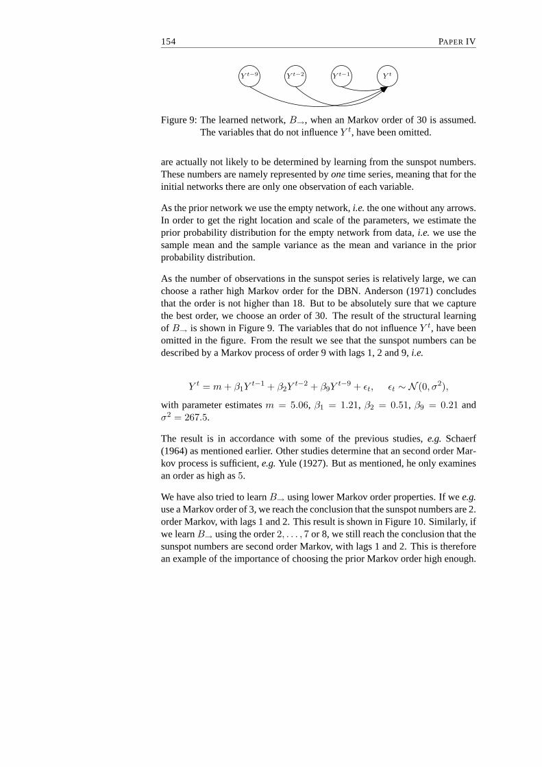
154 PAPER IV
Y t−9 Y t−2 Y t−1 Y t
Figure 9: The learned network,B→, when an Markov order of 30 is assumed.The variables that do not influenceY t, have been omitted.
are actually not likely to be determined by learning from thesunspot numbers.These numbers are namely represented byonetime series, meaning that for theinitial networks there are only one observation of each variable.
As the prior network we use the empty network,i.e. the one without any arrows.In order to get the right location and scale of the parameters, we estimate theprior probability distribution for the empty network from data, i.e. we use thesample mean and the sample variance as the mean and variance in the priorprobability distribution.
As the number of observations in the sunspot series is relatively large, we canchoose a rather high Markov order for the DBN. Anderson (1971) concludesthat the order is not higher than 18. But to be absolutely surethat we capturethe best order, we choose an order of 30. The result of the structural learningof B→ is shown in Figure 9. The variables that do not influenceY t, have beenomitted in the figure. From the result we see that the sunspot numbers can bedescribed by a Markov process of order 9 with lags 1, 2 and 9,i.e.
Y t = m + β1Yt−1 + β2Y
t−2 + β9Yt−9 + ǫt, ǫt ∼ N (0, σ2),
with parameter estimatesm = 5.06, β1 = 1.21, β2 = 0.51, β9 = 0.21 andσ2 = 267.5.
The result is in accordance with some of the previous studies, e.g. Schaerf(1964) as mentioned earlier. Other studies determine that an second order Mar-kov process is sufficient,e.g.Yule (1927). But as mentioned, he only examinesan order as high as5.
We have also tried to learnB→ using lower Markov order properties. If wee.g.use a Markov order of 3, we reach the conclusion that the sunspot numbers are 2.order Markov, with lags 1 and 2. This result is shown in Figure10. Similarly, ifwe learnB→ using the order2, . . . , 7 or 8, we still reach the conclusion that thesunspot numbers are second order Markov, with lags 1 and 2. This is thereforean example of the importance of choosing the prior Markov order high enough.
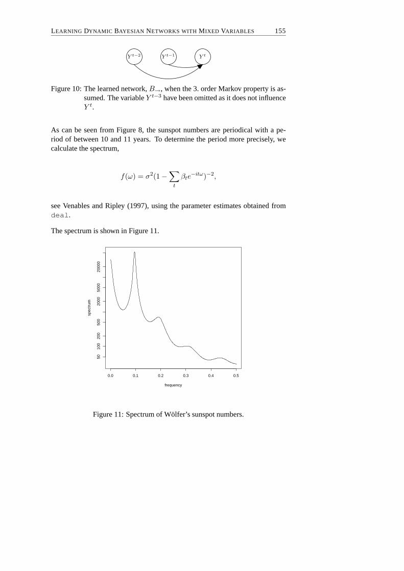
LEARNING DYNAMIC BAYESIAN NETWORKS WITH M IXED VARIABLES 155
Y t−2 Y t−1 Y t
Figure 10: The learned network,B→, when the 3. order Markov property is as-sumed. The variableY t−3 have been omitted as it does not influenceY t.
As can be seen from Figure 8, the sunspot numbers are periodical with a pe-riod of between 10 and 11 years. To determine the period more precisely, wecalculate the spectrum,
f(ω) = σ2(1−∑
t
βte−itω)−2,
see Venables and Ripley (1997), using the parameter estimates obtained fromdeal.
The spectrum is shown in Figure 11.
0.0 0.1 0.2 0.3 0.4 0.5
5010
020
050
020
0050
0020
000
frequency
spec
trum
Figure 11: Spectrum of Wölfer’s sunspot numbers.

156 PAPER IV
There is a peak at frequency 0.096, which corresponds to a period of 1/0.096 =10.40 years. This result is also in accordance with previous studies.
Acknowledgements
This research was supported by Novo Nordisk A/S. Also I wouldlike to thankClaus Dethlefsen for useful discussions and his help with the implementationof the example. Finally, I thank my supervisor Steffen L. Lauritzen for manyvaluable comments.
References
Anderson, T. W. (1971).The Statistical Analysis of Time Series, John Wiley andSons, New York.
Bøttcher, S. G. (2001). Learning Bayesian Networks with Mixed Variables,Ar-tificial Intelligence and Statistics 2001, Morgan Kaufmann, San Francisco,CA, USA, pp. 149–156.
Bøttcher, S. G. and Dethlefsen, C. (2003).deal: A Package for LearningBayesian Networks,Journal of Statistical Software8(20): 1–40.
Bøttcher, S. G., Milsgaard, M. B. and Mortensen, R. S. (1995). Monitoring byusing dynamic linear models - illustrated by tumour markersfor cancer,Master’s thesis, Aalborg University.
Cooper, G. and Herskovits, E. (1992). A Bayesian method for the induction ofprobabilistic networks from data,Machine Learning9: 309–347.
Dean, T. and Kanazawa, K. (1989). A model for reasoning aboutpersistenceand causation,Computational Intelligence5: 142–150.
DeGroot, M. H. (1970). Optimal Statistical Decisions, McGraw-Hill, NewYork.
Friedman, N., Murphy, K. P. and Russell, S. (1998). Learningthe Structure ofDynamic Probabilistic Networks,Proceedings of Fourteenth Conferenceon Uncertainty in Artificial Intelligence, Morgan Kaufmann, San Fran-cisco, CA, USA, pp. 139–147.

LEARNING DYNAMIC BAYESIAN NETWORKS WITH M IXED VARIABLES 157
Geiger, D. and Heckerman, D. (1994). Learning Gaussian Networks,Proceed-ings of Tenth Conference on Uncertainty in Artificial Intelligence, MorganKaufmann, San Francisco, CA, USA, pp. 235–243.
Harrison, P. J. and Stevens, C. F. (1976). Bayesian forecasting,Journal of RoyalStatistics38: 205–247.
Heckerman, D., Geiger, D. and Chickering, D. M. (1995). Learning Bayesiannetworks: The combination of knowledge and statistical data, MachineLearning20: 197–243.
Lauritzen, S. L. (1996).Graphical Models, Clarendon press, Oxford, New York.
Murphy, K. P. (2002).Dynamic Bayesian Networks: Representation, Inferenceand Learning, PhD thesis, University of California, Berkeley.
Schaerf, M. C. (1964). Estimation of the covariance and autoregressive struc-ture of a stationary time series,Technical report, Department of Statistics,Stanford University.
Tong, H. (1996).Non-Linear Time Series, Clarendon Press, Oxford.
Venables, W. N. and Ripley, B. D. (1997).Modern Applied Statistics with S-PLUS, second edn, Springer-Verlag, New York.
West, M. and Harrison, J. (1989).Bayesian Forecasting and Dynamic Models,Springer-Verlag, New York.
Yule, G. U. (1927). On a method for investigating periodicities in disturbedseries with special reference to Wölfer’s sunspot numbers,PhilosophicalTransactions of the Royal Society, Series A226: 267–298.

158 PAPER IV