a uni ed approach to systemic risk measures via acceptance ... · frittelli and rosazza gianin...
TRANSCRIPT
A Unified Approach to Systemic Risk Measures via
Acceptance Sets
Francesca Biagini∗ Jean-Pierre Fouque † Marco Frittelli‡
Thilo Meyer-Brandis§
July 12, 2017
Abstract
We specify a general methodological framework for systemic risk measures
via multi-dimensional acceptance sets and aggregation functions. Existing sys-
temic risk measures can usually be interpreted as the minimal amount of cash
needed to secure the system after aggregating individual risks. In contrast,
our approach also includes systemic risk measures that can be interpreted as
the minimal amount of cash that secures the aggregated system by allocating
capital to the single institutions before aggregating the individual risks. An
important feature of our approach is the possibility of allocating cash accord-
ing to the future state of the system (scenario-dependent allocation). We also
provide conditions which ensure monotonicity, convexity, or quasi-convexity of
our systemic risk measures.
Key Words: Systemic risk, risk measures, acceptance set, aggregation.
Mathematics Subject Classification (2010): 60A99; 91B30; 91G99; 93D99.
∗Department of Mathematics, University of Munich, Theresienstraße 39, 80333 Munich, Ger-
many. [email protected].†Department of Statistics & Applied Probability, University of California, Santa Barbara, CA
93106-3110, [email protected]. Work supported by NSF grants DMS-1107468 and DMS-
1409434.‡Dipartimento di Matematica, Universita degli Studi di Milano, Via Saldini 50, 20133 Milano,
Italy, [email protected].§Department of Mathematics, University of Munich, Theresienstraße 39, 80333 Munich, Ger-
Francesca Biagini and Thilo Meyer-Brandis thank the Frankfurt Institute for Risk Management
and Regulation and the Europlace Institute of Finance for support.
Part of this research was performed while F. Biagini, M. Frittelli and T. Meyer-Brandis were visit-
ing the University of California Santa Barbara, and the paper was finalized while the four authors
were visiting the Institute for Pure and Applied Mathematics (IPAM), which is supported by the
National Science Foundation.
We would like to thank two anonymous reviewers for their suggestions, which contributed to improve
the paper. We wish to thank Francesco Rotondi for his help with the simulations, and Riccardo
Bassani.
1
1 Introduction
The financial crisis has dramatically demonstrated that traditional risk manage-
ment strategies of financial systems, which predominantly focus on the solvency of
individual institutions as if they were in isolation, insufficiently capture the per-
ilous systemic risk that is generated by the interconnectedness of the system entities
and the corresponding contagion effects. This has brought awareness of the urgent
need for novel approaches that capture systemic riskiness. A large part of the cur-
rent literature on systemic financial risk is concerned with the modeling structure
of financial networks, the analysis of the contagion and the spread of a potential
exogenous (or even endogenous) shock into the system. For a given financial (possi-
bly random) network and a given random shock one then determines the “cascade”
mechanism which generates possibly many defaults. This mechanism often requires
a detailed description of the balance sheet of each institution; assumptions on the
interbank network and exposures, on the recovery rate at default, on the liquidation
policy; the analysis of direct liabilities, bankruptcy costs, cross-holdings, leverage
structures, fire sales, and liquidity freezes.
These approaches may be relevant also from the viewpoint of a policy maker that
has to intervene and regulate the banking system to reduce the risk that, in case of an
adverse (local) shock, a substantial part or even the complete system breaks down.
However, once such a model for the financial network has been identified and the
mechanism for the spread of the contagion determined, one still has to understand
how to compare the possible final outcomes in a reasonable way or, in other words,
how to measure the risk carried by the global financial system. This is the focus
of our approach, as we measure the risk embedded in a financial system taking as
primitive the vector X = (X1, . . . , XN ) of changes in the value to the horizon T ,
where Xi is interpreted as the future gain if Xi is positive or as the future loss if Xi
is negative of institution i. Such profit and loss1 is typically uncertain and therefore
it will be modeled by a random variable Xi(ω) on some space of possible scenarios
ω ∈ Ω.
Our approach is close in spirit to the “classical” conceptual framework of univari-
ate monetary risk measures initiated by the seminal paper by Artzner et al. (1999)
and the aim of this paper is to extend and generalize such univariate framework to
a multivariate setting that takes into account not only one single institution but a
complete system. More precisely, we specify a general methodological framework to
design systemic risk measures via multivariate acceptance sets which is very flexible
and comprises most of the existing systemic risk measures proposed in the literature.
In particular it contains the popular class of systemic risk measures that can be inter-
preted as the minimal amount of cash needed to secure the system after aggregating
the N individual risks X into some univariate system-wide risk by some aggrega-
1Even though we defined Xi as the change in the portfolio’s ith value, one may also interpret
Xi as the future value of firm i, as done for example in the seminal paper Artzner et al. (1999).
2

tion rule, see Chen et al. (2013), Kromer et al. (2013), Hoffmann et al. (2015a) and
Hoffmann et al. (2015b) for a structural analysis of this class. However, beyond this
class our approach offers various other interesting ways and extensions to design
systemic risk measures. In particular, one of its most interesting features is that it
also includes systemic risk measures that can be interpreted as the minimal amount
of cash that secures the aggregated system by allocating capital to the single insti-
tutions before aggregating the individual risks. Further, we include the possibility
of generalized (random) admissible assets to secure the system which allows for the
allocation of cash according to the future state of the system (scenario-dependent
allocation). This is particularly interesting from the viewpoint of a lender of last
resort who might be interested in determining today the total capital needed to
secure the system and then, in the future, can inject the capital where it serves the
most in response to which scenario has been realized. Throughout the paper we will
pay special attention to the analysis and examples of this family of systemic risk
measures. The examples will also show that scenario-dependent allocations permit
to take into account in a natural way the dependence structure of the risk vector X.
There is a huge literature on systemic risk, which takes into account different
points of view on the subject. For empirical studies on banking networks, we refer
for example to Craig and von Peter (2014), Boss et al. (2004) and Cont et al.
(2013). Interbank lending has been studied via interacting diffusions and mean
field approach in several papers like Fouque and Sun (2013), Fouque and Ichiba
(2013), Carmona et al. (2015), Kley et al. (2015), Battiston et al. (2012). Among
the many contributions on systemic risk modeling, we mention here the classical
contagion model proposed by Eisenberg and Noe (2001), the default model of Gai
and Kapadia (2010b), the illiquidity cascade models of Gai and Kapadia (2010a),
Hurd et al. (2014) and Lee (2013), the asset fire sale cascade model by Cifuentes
et al. (2005) and Caccioli et al. (2012), as well as the model in Awiszus and Weber
(2015) that additionally includes cross-holdings. Further works on network modeling
are Amini et al. (2013), Rogers and Veraart (2013), Amini et al. (2014), Gleeson
et al. (2013), Battiston and Caldarelli (2013), Detering et al. (2016a) and Detering
et al. (2016b). See also the references therein. For an exhaustive overview on the
literature on systemic risk we refer the reader to the recent volumes of Hurd (2016)
and of Fouque and Langsam (2013).
The structure of the paper is the following. In Section 2, starting from the well-
known formulation of univariate risk measures, we gradually motivate and develop
our framework for systemic risk measures defined via multivariate acceptance sets.
In Section 3 we lay the theoretical foundations of our approach. In particular we
study the properties of monotonicity and quasi-convexity (or convexity) of systemic
risk measures. In Section 4 we analyze various families of systemic risk measures
where the risk measurement is defined by aggregating the vector of risk factors
into some system-wide univariate risk and then testing acceptability with respect
to some one-dimensional acceptance set as in (2.16). Section 5 investigates the
3
interesting class of systemic risk measures that are defined in terms of a set C of
scenario-dependent allocations as in (2.10). Then we present two concrete examples
within this class of systemic risk measures in Sections 6 and 7. In Section 6 we
look at Gaussian systems and consider both deterministic cash allocations as well
as a certain class of random cash allocations. In Section 7 we introduce an example
on a finite probability space, where we are able to compute explicitly systemic risk
measures for very general scenario dependent cash allocations.
2 Systemic risk measures
2.1 From one-dimensional to N-dimensional risk profiles
In this subsection we review the literature on risk measurement based on acceptance
sets, both in the traditional one-dimensional setting as well as in the case of N
interacting financial institutions. Here we denote with L0(RN ) := L0(Ω,F ;RN ),
N ∈ N, the space of RN -valued random variables on the probability space (Ω,F ,P).
Traditional risk management strategies evaluate the risk η(Xi) of each institution
i ∈ 1, ...N by applying a univariate monetary risk measure η to the single financial
position Xi. A monetary risk measure (see Follmer and Schied (2004)) is a map
η : L0(R) → R that can be interpreted as the minimal capital needed to secure a
financial position with payoff X ∈ L0(R), i.e., the minimal amount m ∈ R that
must be added to X in order to make the resulting (discounted) payoff at time T
acceptable
(2.1) η(X) := infm ∈ R | X +m ∈ A,
where the acceptance set A ⊆ L0(R) is assumed to be monotone, i.e., X ≥ Y ∈ Aimplies X ∈ A. In addition to decreasing monotonicity, the characterizing feature
of these maps is the cash additivity property
(2.2) η(X +m) = η(X)−m, for all m ∈ R.
Under the assumption that the set A is convex (resp. is a convex cone) the maps in
(2.1) are convex (resp. convex and positively homogeneous) and are called convex
(resp. coherent) risk measures, see Artzner et al. (1999), Follmer and Schied (2002),
Frittelli and Rosazza Gianin (2002). The principle that diversification should not
increase the risk is mathematically translated not necessarily with the convexity
property but with the weaker condition of quasiconvexity
η(λX + (1− λ)Y ) ≤ η(X) ∨ η(Y ).
As a result, in Cerreia-Vioglio et al. (2010) and Frittelli and Maggis (2014), the only
properties assumed in the definition of a quasi-convex risk measure are monotonicity
and quasiconvexity. Such risk measures can always be written as
(2.3) η(X) := infm ∈ R | X ∈ Am,
4

where each set Am ⊆ L0(R) is monotone and convex, for each m. Here Am is inter-
preted as the class of payoffs carrying the same risk level m. Contrary to the convex,
cash additive case where each random variable is binary cataloged as acceptable or
as not acceptable, in the quasi-convex case one admits various degrees of accept-
ability, described by the risk level m, see Cherny and Madan (2009). Furthermore,
in the quasi-convex case the cash additivity property will not hold in general and
one loses a direct interpretation of m as the minimal capital required to secure the
payoff X, but preserves the interpretation of Am as the set of positions acceptable
for the given risk level m. By selecting Am := A−m, the risk measure in ( 2.1) is
clearly a particular case of the one in (2.3).
However, as mentioned in the introduction, traditional risk management by uni-
variate risk measures insufficiently captures systemic risk, and a rapidly growing
literature is concerned with designing more appropriate risk measures for financial
systems. A systemic risk measure is then a map ρ : L0(RN ) → R that evaluates
the risk ρ(X) of the complete system X = (X1, ..., XN ). Most of the systemic risk
measures in the existing literature are of the form
(2.4) ρ(X) = η(Λ(X)),
where η : L0(R)→ R is a univariate risk measure and
Λ : RN → R
is an aggregation rule that aggregates the N -dimensional risk factor X into a uni-
variate risk factor Λ(X). Some examples of aggregation rules found in the literature
are the following:
i) One of the most common ways to aggregate multivariate risk is to simply sum
the single risk factors: Λ(x) =∑N
i=1 xi, x = (x1, ..., xN ) ∈ RN . Also, in the litera-
ture on systemic risk measures there are examples using this aggregation rule, like
for example the Systemic Expected Shortfall introduced in Acharya et al. (2010),
or the Contagion Value at Risk (CoVaR) introduced in Adrian and Brunnermeier
(2011). However, while summing up profit and loss positions might be reasonable
from the viewpoint of a portfolio manager where the portfolio components com-
pensate each other, this aggregation rule seems inappropriate for a financial system
where cross-subsidization between institutions is rather unrealistic. Further, if the
sum was a suitable aggregation of risk in financial systems, then the traditional
approach of applying a univariate coherent risk measure η to the single risk fac-
tors would be sufficiently prudent in the sense that by sub-linearity it holds that
η(∑N
i=1Xi) ≤∑N
i=1 η(Xi).
ii) One possible aggregation that takes the lack of cross-subsidization between
financial institutions into account is to sum up losses over a threshold only: Λ(x) =∑Ni=1−(xi−di)−, where x− := −min(x, 0). This kind of aggregation is for example
used in Huang et al. (2009), Lehar (2005). See also Brunnermeier and Cheridito
5

(2013) for an extension of this type of aggregation rule that also considers a certain
effect of gains, as Λ(x) =∑N
i=1−αix−i +
∑Ni=1 βi(xi − vi)+ for some αi, βi, vi ∈ R+,
i = 1, · · · , N .
iii) Beside the lack of cross-subsidization in a financial system, the aggregation
rule may also account for contagion effects that can considerably accelerate sys-
temwide losses resulting from an initial shock. Motivated by the structural conta-
gion model of Eisenberg and Noe (2001), Chen et al. (2013) introduce an aggregation
function that explicitly models the net systemic cost of the contagion in a financial
system by defining the aggregation rule
ΛCM (x) = minyi≥xi+
∑Nj=1 Πijyj ,∀i=1,··· ,N, y∈RN
+
N∑i=1
yi
.
Here, Π = (Πij)i,j=1,··· ,N represents the relative liability matrix, i.e.,firm i has to
pay the proportion Πij of its total liabilities to firm j.
An axiomatic characterization of systemic risk measures of the form (2.4) on a
finite state space is provided in Chen et al. (2013), see also Kromer et al. (2013)
for the extension to a general probability space and Hoffmann et al. (2015a) for a
further extension to a conditional setting. Also, in these references further examples
of possible aggregation functions can be found.
Remark 2.1 The above examples of aggregation functions clarify that, depending
on the model and aggregation approach, the primitive X in our systemic risk measure
might be interpreted as future profit and loss positions. In the context of the first
two aggregation rules, X denotes the vector that already includes the potential risk
of a contagion spread into the system. Thus, in this situation X already includes a
reduced form modeling of the potential contagion channels. On the other hand, in
the context of the third aggregation rule, X is interpreted as the future profit and
loss positions before the contagion takes place and the contagion mechanism will
explicitly be embedded in the risk measure via the aggregation function. Either way,
our scope is to provide a consistent criterion to assess whether one possible vector
X is riskier than another.
If η in (2.4) is a monetary risk measure it follows from (2.1) that we can rewrite
the systemic risk measure ρ in (2.4) as
(2.5) ρ(X) := infm ∈ R | Λ(X) +m ∈ A .
Thus, presuming Λ(X) represents some loss, systemic risk can again be interpreted
as the minimal cash amount that secures the system when it is added to the total
aggregated system loss Λ(X). If Λ(X) does not allow for an interpretation as cash,
the risk measure in (2.5) has to be understood as some general risk level of the system
6
rather than some capital requirement. Similarly from (2.3), if η is a quasi-convex
risk measure the systemic risk measure ρ in (2.4) can be rewritten as
(2.6) ρ(X) := infm ∈ R | Λ(X) ∈ Am.
Again, one first aggregates the risk factors via the function Λ and in a second step
one computes the minimal risk level associated to Λ(X).
Example 2.2 Most of the existing systemic risk measures in the literature can be
embedded in our framework by the formulation (2.5) (first aggregation, then applying
a univariate risk measure). For example, the DIP (Black et al. (2016), see also
Huang et al. (2009)) given by EQ[∑
iXi1∑
iXi≤Lmin] is obtained from (2.5) by
putting Λ(x) =∑
i xi1∑
i xi≤Lmin and taking A as the acceptance set associated to
the univariate risk measure η given by the expected shortfall with respect to the risk
neutral measure Q. So DIP measures the risk-neutral expected systemic losses that
exceed a certain threshold Lmin.
The CoVar (Adrian and Brunnermeier (2011)) with respect to institution j is
given by V aR(∑
iXi|Xj = V aR(Xj)). This can be computed for (X1, ..., Xn) from
(2.5) by putting Λ(x) =∑
i xi and taking A as the acceptance set associated to the
univariate risk measure η given by the VaR with respect to the conditional probability
distribution given the event Xj = V aR(Xj).The MES (Acharya et al. (2010)) with respect to institution j is defined as
E[Xj |∑
iXi ≤ V aR(∑
iXi)]. Here, Λ(x) = xj and A is the acceptance set as-
sociated to the univariate risk measure η given by the expectation with respect to
the condition probability distribution given the event ∑
iXi ≤ V aR(∑
iXi). Note
that DIP measures systemic risk in an unconditional setting, i.e., it takes the prob-
ability of a systemic loss into account, while CoVar and MES measure systemic risk
conditional on the event that a loss has occurred. More precisely, CoVar measures
the impact of realized distress of institution j on the system, while MES measures
the impact of realized distress of the system on institution j. For other examples of
systemic risk measures, we also refer to Benoit et al. (2016).
While the approach prescribed in (2.5) and (2.6) defines an interesting class of
systemic risk measures, one could think of meaningful alternative or extended pro-
cedures of measuring systemic risk not captured by (2.5) or (2.6). In the following
subsections, we extend the conceptual framework for systemic risk measures via ac-
ceptance sets step by step in order to gradually include certain novel key features
before we reach our general formulation of systemic risk measures via multivariate
acceptance sets.
2.2 First add capital, then aggregate
The interpretation of (2.5) to measure systemic risk as minimal capital needed to
secure the system after aggregating individual risks is for example meaningful in the
7

situation where some kind of rescue fund shall be installed to repair damage from
systemic loss. However, for instance from the viewpoint of a regulator who has the
possibility to intervene at the level of the single institutions before contagion effects
generate further losses, it might be more relevant to measure systemic risk as the
minimal capital that secures the aggregated system by injecting the capital into the
single institutions before aggregating the individual risks. This way of measuring
systemic risk can be expressed by
(2.7) ρ(X) := infN∑i=1
mi |m = (m1, ...,mN ) ∈ RN , Λ(X + m) ∈ A .
Here, the amount mi is added to the financial position Xi of institution i ∈ 1, ..., Nbefore the corresponding total loss Λ(X + m) is computed. For example, consider-
ing the aggregation function ΛCM from above it becomes clear that injecting cash
first might prevent further losses that would be generated by contagion effects. The
systemic risk is then measured as the minimal total amount∑N
i=1mi injected into
the institutions to secure the system.
Independently, a related concept in the context of set-valued systemic risk measures
has been developed in Feinstein et al. (2015). They also use acceptance sets in
building the notion of systemic risk measures and admit the possibility of injecting
capital before aggregating individual risks (aggregation mechanism sensitive to cap-
ital levels, in the language of Feinstein et al. (2015)). However, the two approaches
are difficult to compare essentially because they rely on different risk measures (set
valued risk measures in Feinstein et al. (2015) versus real valued risk measures in our
paper). Furthermore, only deterministic allocations are allowed in Feinstein et al.
(2015), while we also admit scenario-dependent allocations. Notice also that Fein-
stein et al. (2015) recognize the need for extracting a real valued risk measure with
minimal properties (called “orthant risk measure”) from a set valued risk measure.
Even in this form, such orthant risk measure can not include our formulation of risk
measures, for the reason explained above. As illustrated in the Examples of Sections
6 and 7, one of the consequences of our approach is that the dependence structure
of the risk vector X can be taken into account due to the flexibility of selecting
scenario-dependent allocations, a feature illustrated in the next section and absent
in Feinstein et al. (2015).
Remark 2.3 Mainly, the literature on systemic risk can be divided into contribu-
tions to two different challenges: The first one concerns the definition and identifi-
cation of an appropriate measure of the overall systemic risk in a financial system.
Having identified the systemic risk, a second question is then how to allocate fair
shares of the total systemic risk to the individual institutions and to establish a
ranking of the institutions in terms of systemic relevance. The main purpose of this
paper is to contribute to the former question and to introduce a general methodology
to design systemic risk measures. However, an interesting question that arises for
8
a systemic risk measure defined as in (2.7) is whether it delivers, in addition to a
measure of total systemic risk, also a potential ranking of the institutions. Indeed, if
m∗ = (m∗1, ...,m∗N ) is such that ρ(X) =
∑Ni=1m
∗i , one could be tempted to interpret
the ordered cash allocations m∗i1 ≥ ... ≥ m∗iN as a ranking of individual risk shares,
and the essential question is whether this ranking can be justified as being fair. We
will touch on this aspect in the Examples in Sections 6 and 7, but a comprehensive
analysis of this interesting and challenging question is beyond the scope of this paper
and is left for future research.
2.3 First add scenario-dependent allocation, then aggregate
One main novelty of this paper is that we want to allow for the possibility of adding
to X not merely a vector m = (m1, ...,mN ) ∈ RN of cash but a random vector
Y ∈ C ⊆ L0(RN )
which represents admissible assets with possibly random payoffs at time T , in the
spirit of Frittelli and Scandolo (2006). To each Y ∈ C we assign a measure π(Y) of
the risk (or cost) associated to Y determined by a monotone increasing map
(2.8) π : C → R .
This leads to the following extension of (2.7)
(2.9) ρ(X) := infπ(Y) ∈ R | Y ∈ C, Λ(X + Y) ∈ A .
Considering a general set C in (2.9) allows for more general measurement of systemic
risk than the cash needed today for each institution to secure the system. For
example, C could be a set of (vectors of) general admissible financial assets that
can be used to secure a system by adding Y to X component-wise, and π(Y) is a
valuation of Y. Another example that we analyze in more detail in this paper and
which is particularly interesting from the viewpoint of a lender of last resort is the
following class of sets C
(2.10) C ⊆ Y ∈ L0(RN ) |N∑n=1
Y n ∈ R =: CR,
and π(Y) =∑N
n=1 Yn. Here the notation
∑Nn=1 Y
n ∈ R means that∑N
n=1 Yn is
equal to some deterministic constant in R, even though each single Y n, n = 1, · · · , N ,
is a random variable. Then, as in (2.7) the systemic risk measure
(2.11) ρ(X) := infN∑n=1
Y n | Y ∈ C, Λ(X + Y) ∈ A
can still be interpreted as the minimal total cash amount∑N
n=1 Yn ∈ R needed
today to secure the system by distributing the cash at the future time T among
9
the components of the risk vector X. However, contrary to (2.7), in general the
allocation Y i(ω) to institution i does not need to be decided today, but depends on
the scenario ω that has been realized at time T . This corresponds to the situation of
a lender of last resort who is equipped with a certain amount of cash today and who
will allocate it according to where it serves the most depending on the scenario that
has been realized at T . Restrictions on the possible distributions of cash are given
by the set C. For example, for C = RN the situation corresponds to (2.7) where
the distribution is already determined today, while for C = CR the distribution can
be chosen completely freely depending on the scenario ω that has been realized
(including negative amounts, i.e., withdrawals of cash from certain components).
Section 5, 6, and 7 will be devoted to the analysis and concrete examples of the class
of systemic risk measures using a set C as in (2.10). We will see that in the case C =
CR where unrestricted cross-subsidization is possible, the canonical way of measuring
systemic risk measure is of the form (2.4) with aggregation rule Λ(x) =∑N
i=1 xi, x ∈RN , i.e., to apply a univariate risk measure to the sum of the risk factors. Another
interesting feature of allowing scenarios depending allocations of cash Y ∈ C ⊆ CR is
that in general the systemic risk measure will take the dependence structure of the
components of X into account even though acceptable positions might be defined in
terms of the marginal distributions ofXi, i = 1, ..., N only. For instance, the example
in Section 6 employs the aggregation rule Λ(x) =∑N
i=1−(xi−di)−, x ∈ RN , di ∈ R,
for i = 1, · · · , N , and the acceptance set Aγ := Z ∈ L0(R) | E[Z] ≥ γ , γ ∈ R.
Then a risk vector Z = (Z1, ..., ZN ) ∈ L0(RN ) is acceptable if and only if Λ(Z) ∈ A,
i.e.,N∑i=1
−E[(Zi − di)−] ≥ γ ,
which only depends on the marginal distributions of Z. Thus, if we choose C =
RN then it is obvious that in this case also the systemic risk measure ρ(X) in
(2.11) depends on the marginal distributions of X only. If, however, one allows for
more general allocations Y ∈ C ⊆ CR that might differ from scenario to scenario
the systemic risk measure will in general depend on the multivariate distribution
of X, as it can play on the dependence of the components of X to minimize the
costs. In the examples of Section 6 and 7 this feature is explicitly shown, as we
provide a comparison between the risk measure computed with deterministic and
with scenario-dependent allocation.
2.4 Multi-dimensional Acceptance Sets
Until now, we have always defined systemic risk measures in terms of acceptability
of an aggregated, one-dimensional system-wide risk. However, not necessarily every
relevant systemic risk measure is of this aggregated type. Consider for instance the
popular approach (though possibly problematic for financial systems as explained
10
above) to add single univariate monetary risk measures ηi, i = 1, ..., N , i.e.,
(2.12) ρ(X) :=N∑i=1
ηi(Xi) .
In general, the systemic risk measure in (2.12) cannot be expressed in the form
(2.9). Denoting by Ai ⊆ L0(R) the acceptance set of ηi, i = 1, ..., N , one easily sees
from (2.1), however, that ρ in (2.12) can be written in terms of the multivariate
acceptance set A1 × ...× AN
ρ(X) := infN∑i=1
mi | m = (m1, ...,mN ) ∈ RN , X + m ∈ A1 × ...× AN .
Motivated by this example, we extend (2.9) to the formulation of systemic risk
measures as the minimal cost of admissible asset vectors Y ∈ C that, when added to
the vector of financial positions X, makes the augmented financial positions X + Y
acceptable in terms of a general multidimensional acceptance set A ⊆ L0(RN )
(2.13) ρ(X) := infπ(Y) ∈ R | Y ∈ C, X + Y ∈ A .
Note that by putting A :=Z ∈ L0(RN ) | Λ(Z) ∈ A
, Definition (2.9) is a special
case of (2.13). Also, in analogy to (2.2), we remark that for linear valuation rules π
the systemic risk measure given in (2.13) exhibits an extended type of cash invariance
in the sense that
(2.14) ρ(X + Y) = ρ(X) + π(Y)
for Y ∈ C such that Y′ ±Y ∈ C for all Y′ ∈ C, see Frittelli and Scandolo (2006).
2.5 Degree of Acceptability
In order to reach the final, most general formulation of systemic risk measures, we
assign, in analogy to (2.3), to each Y ∈ C a set AY ⊆ L0(RN ) of risk vectors that are
acceptable for the given (random) vector Y, and define the systemic risk measure
by
(2.15) ρ(X) := infπ(Y) ∈ R | Y ∈ C, X ∈ AY .
Note that analogously to the one-dimensional quasi-convex case (2.3), the systemic
risk measures (2.15) cannot necessarily be interpreted as cash added to the system
but in general represent some minimal aggregated risk level π(Y) at which the
system X is acceptable. The approach in (2.15) is very flexible and unifies a variety
of different features in the design of systemic risk measures. In particular, it includes
all previous cases if we set
AY := A−Y,
11

where the set A ⊆ L0(RN ) represents acceptable risk vectors. Then obviously (2.13)
is obtained from (2.15).
Another advantage of the formulation in terms of general acceptance sets is the
possibility to design systemic risk measures via general aggregation rules. Indeed
the formulation (2.15) includes the case
(2.16) ρ(X) := infπ(Y) ∈ R | Y ∈ C, Θ(X,Y) ∈ A,
where Θ : L0(RN )×C → L0(R) denotes some aggregation function jointly in X and
Y. Just select AY :=Z ∈ L0(RN ) | Θ(Z,Y) ∈ A
. In particular, (2.16) includes
both the case “injecting capital before aggregation”as in (2.7) and (2.9) by putting
Θ(X,Y) =Λ(X + Y), and the case “aggregation before injecting capital”as in (2.5)
by putting Θ(X,Y) :=Λ1(X)+Λ2(Y), where Λ1 : L0(RN ) → L0(R) is an aggrega-
tion function and Λ2 : C → L0(R) could be, for example, the discounted cost of Y.
Also, again in analogy to the one-dimensional case (2.3), the more general depen-
dence of the acceptance set on Y in (2.15) allows for multi-dimensional quasi-convex
risk measures. Note that the cash additivity property (2.14) is then lost in general.
3 Definition of Systemic Risk Measures and Properties
In this Section we provide the definitions and properties of the systemic risk measures
in our setting. As in Section 2, we consider the set of random vectors
L0(RN ) := X = (X1, . . . , XN ) | Xn ∈ L0(Ω,F ,P), n = 1, · · · , N,
on the probability space (Ω,F ,P). We assume that L0(RN ) is equipped with an
order relation such that it is a vector lattice. One such example is provided by
the order relation: X1 X2 if Xi1 ≥ Xi
2 for all components i = 1, ..., N , where for
random variables in L0(R), the order relation is determined by P−a.s inequality.
Definition 3.1 Let X1, X2 ∈ L0(RN ).
1. A set A ⊂ L0(RN ) is -monotone if X1 ∈ A and X2 X1 implies X2 ∈ A.
2. A map f : L0(RN ) → L0(R) is -monotone decreasing if X2 X1 implies
f(X1) ≥ f(X2). Analogously for functions f : L0(RN )→ R.
3. A map f : L0(RN )→ R is quasi-convex if
f(λX1 + (1− λ)X2) ≤ f(X1) ∨ f(X2).
A vector X = (X1, . . . , XN ) ∈ L0(RN ) denotes a configuration of risky factors at a
future time T associated to a system of N entities. Let
C ⊆ L0(RN ).
12
To each Y ∈ C we assign a set AY ⊆ L0(RN ). The set AY represents the risk
vectors X that are acceptable for the given random vector Y. Let also consider a
map
π : C → R ,
so that π(Y) represents the risk (or cost) associated to Y.
We now introduce the concept of monotone and (quasi-) convex systemic risk mea-
sure.
Definition 3.2 The systemic risk measure associated with C,AY and π is a map
ρ : L0(RN )→ R := R ∪ −∞ ∪ ∞, defined by
(3.1) ρ(X) := infπ(Y) ∈ R | Y ∈ C, X ∈ AY .
Moreover ρ is called a quasi-convex (resp. convex) systemic risk measure if it is
-monotone decreasing and quasi-convex (resp. convex on ρ(X) < +∞).
In other words, the systemic risk of a random vector X is measured by the minimal
risk (cost) of those random vectors Y that make X acceptable.
We now focus on several examples of systemic risk measures of the type (3.1). To
guarantee that such maps are finite valued one could consider their restriction to
some vector subspaces of L0(RN ) (for examples Lp(RN ), p ∈ [1,∞]) and impose
further conditions on the defining ingredients (π, C, AY) of ρ. For example, suppose
that C and AY satisfy the two conditions
1.m1 ∈RN | m ∈ R+, 1 := (1, ...,1)
⊆ C,
2. −m1 ∈ Am1 and Am1 is a monotone set for each m ∈ R+,
then ρ : L∞(RN ) → R defined by (3.1) satisfies ρ(X) < +∞ for all X ∈ L∞(RN ).
Indeed, for m := maxi ‖Xi‖∞, X ≥ −m1 ∈ Am1 implies that X ∈Am1 and π(m1) <
+∞.
Clearly, other sufficient conditions may be obtained in each specific example of
systemic risk measures considered in the subsequent Sections.
We opt to accept the possibility that such maps ρ may assume values ±∞. However,
it is not difficult to find simple sufficient conditions assuring that the systemic risk
measure in (3.1) is proper (not identically equal to +∞). One such example is the
condition
if 0 ∈ C and 0 ∈ A0 then ρ(0) ≤ π(0) < +∞,
and in this case we can always obtain ρ(0) = 0 by replacing ρ(·) with ρ(·)−ρ(0). We
now consider the “structural properties” (i.e., monotonicity, quasiconvexity, convex-
ity) of our systemic risk measures and introduce two sets of conditions (properties
(P1), (P2) and (P3) below and the alternative properties (P2a) and (P3a) ) that
13

guarantee that the map in (3.1) is a quasi-convex (or convex) risk measure. In Sec-
tion 4 we show that these sets of conditions can be easily checked in some relevant
examples of maps in the form (3.1), where the set AY is determined from aggrega-
tion and one-dimensional acceptance sets.
We introduce the following properties:
(P1) For all Y ∈ C the set AY ⊂ L0(RN ) is -monotone.
(P2) For all m ∈ R, for all Y1,Y2 ∈ C such that π(Y1) ≤ m and π(Y2) ≤ m
and for all X1 ∈ AY1 , X2 ∈ AY2 and all λ ∈ [0, 1] there exists Y ∈ C such
that π(Y) ≤ m and λX1 + (1− λ)X2 ∈ AY.
(P3) For all Y1,Y2 ∈ C and all X1 ∈ AY1 , X2 ∈ AY2 and all λ ∈ [0, 1] there
exists Y ∈ C such that π(Y) ≤ λπ(Y1)+(1−λ)π(Y2) and λX1 +(1−λ)X2 ∈AY.
It is clear that property (P3) implies property (P2). Moreover, we have
Lemma 3.3 i) If the systemic risk measure ρ defined in (3.1) satisfies the prop-
erties (P1) and (P2), then ρ is -monotone decreasing and quasi-convex.
ii) If the systemic risk measure ρ defined in (3.1) satisfies the properties (P1) and
(P3), then ρ is -monotone decreasing and convex on ρ(X) < +∞.
Proof. Set
B(X) :=Y ∈ C | X ∈ AY
.
First assume that property (P1) holds and w.l.o.g. suppose X2 X1 and B(X1) 6=∅. Then property (P1) implies that if X1 ∈ AY and X2 X1 then: B(X1) ⊆ B(X2).
Hence
ρ(X1) = infπ(Y) | Y ∈ B(X1) ≥ infπ(Y) | Y ∈ B(X2) = ρ(X2)
so that ρ is -monotone decreasing.
i) Now assume that property (P2) holds and let X1,X2 ∈ L0(RN ) be arbitrarily
chosen. For the quasi-convexity we need to prove, for any m ∈ R, that
ρ(X1) ≤ m and ρ(X2) ≤ m⇒ ρ(λX1 + (1− λ)X2) ≤ m.
By definition of the infimum in the definition of ρ(Xi), ∀ε > 0 there exist
Yi ∈ C such that Xi ∈ AYi and
π(Yi) ≤ ρ(Xi) + ε ≤ m+ ε, i = 1, 2.
Take any λ ∈ [0, 1]. Property (P2) guarantees the existence of Z ∈ C such that
π(Z) ≤ m+ ε and λX1 + (1− λ)X2 ∈ AZ. Hence
ρ(λX1 + (1− λ)X2) = infπ(Y) | Y ∈ C, λX1 + (1− λ)X2 ∈ AY≤ π(Z) ≤ m+ ε.
As this holds for any ε > 0, we obtain the quasi-convexity.
14
ii) Assume that property (P3) holds and that X1,X2 ∈ L0(RN ) satisfy ρ(Xi) < +∞.
Then B(Xi) 6= ∅ and, as before, ∀ε > 0 there exists Yi ∈ L0(RN ) such that
Yi ∈ C, Xi ∈ AYi and
(3.2) π(Yi) ≤ ρ(Xi) + ε, i = 1, 2.
By property (P3) there exists Z ∈ C such that π(Z) ≤ λπ(Y1) + (1−λ)π(Y2)
and λX1 + (1− λ)X2 ∈ AZ. Hence
ρ(λX1 + (1− λ)X2) = infπ(Y) | Y ∈ C, λX1 + (1− λ)X2 ∈ AY≤ π(Z) ≤ λπ(Y1) + (1− λ)π(Y2)
≤ λρ(X1) + (1− λ)ρ(X2) + ε,
from (3.2). As this holds for any ε > 0, the map ρ is convex on ρ(X) < +∞.
We now consider the following alternative properties:
(P2a) For all Y1,Y2 ∈ C, X1 ∈ AY1 , X2 ∈ AY2 and λ ∈ [0, 1] there exists
α ∈ [0, 1] such that λX1 + (1− λ)X2 ∈ AαY1+(1−α)Y2 .
(P3a) For all Y1,Y2 ∈ C, X1 ∈ AY1 , X2 ∈ AY2 and λ ∈ [0, 1] it holds that
λX1 + (1− λ)X2 ∈ AλY1+(1−λ)Y2 .
It is clear that property (P3a) implies property (P2a). Furthermore we introduce
the following properties for C and π:
(P4) C is convex,
(P5) π is quasi-convex,
(P6) π is convex.
We have the following
Lemma 3.4 i) Under the conditions (P1), (P2a), (P4), and (P5) the map ρ
defined in (3.1) is a quasi-convex systemic risk measure.
ii) Under the conditions (P1), (P3a) , (P4) and (P6) the map ρ defined in (3.1)
is a convex systemic risk measure.
Proof.
i) It follows from Lemma 3.3 and the fact that the properties (P2a), (P4), and
(P5) imply (P2). Indeed, let Y1,Y2 ∈ C such that π(Y1) ≤ m, π(Y2) ≤ m and
let X1 ∈ AY1 , X2 ∈ AY2 and λ ∈ [0, 1]. Then there exists α ∈ [0, 1] such that
λX1 + (1− λ)X2 ∈ AαY1+(1−α)Y2 . If we set: Y :=αY1 + (1− α)Y2 ∈ C then
λX1 + (1− λ)X2 ∈ AY and π(αY1 + (1− α)Y2) ≤ max(π(Y1), π(Y2)) ≤ m.
15

ii) It follows from Lemma 3.3 and the fact that the properties (P3a) , (P4), and
(P6) imply (P3). Indeed, let Y1,Y2 ∈ C and let X1 ∈ AY1 , X2 ∈ AY2 and
λ ∈ [0, 1]. If we set: Y :=λY1 + (1 − λ)Y2 ∈ C then λX1 + (1 − λ)X2 ∈ AY
and π(Y) ≤ λπ(Y1) + (1− λ)π(Y2).
4 Systemic Risk Measures via Aggregation and One-
dimensional Acceptance Sets
In this Section we study four classes of systemic risk measures in the form (3.1),
which differ from each other by the definition of their aggregation functions and
their acceptance sets. However, these four classes, defined in equations (4.2), (4.3),
(4.6), (4.7), all satisfy the structural properties of monotonicity and quasi-convexity
(or convexity). We consider the following definitions and assumptions, which will
hold true throughout this Section:
1. the aggregation functions are
Λ : L0(RN )× C → L0(R),
Λ1 : L0(RN )→ L0(R),
and we assume that Λ1 is -increasing and concave;
2. the acceptance family
(Bx)x∈R
is an increasing family with respect to x and each set Bx ⊆ L0(R) is assumed
monotone and convex;
3. the acceptance subset
A ⊆ L0(R)
is assumed monotone and convex.
The convexity of the acceptance set A ⊆ L0(R) (or of the acceptance family (Bx)x∈R)
are the standard conditions which have been assumed as the origin of the theory
of risk measures. The concavity of the aggregation functions is justified, not only
from the many relevant examples in literature, but also by the preservation of the
convexity from one dimensional acceptance sets to multi-dimensional ones. Indeed,
let Θ : L0(RN ) → L0(R) be an aggregation function, A ⊆ L0(R) a one dimensional
acceptance set and define A ⊆ L0(RN ) as the inverse image A := Θ−1(A). Suppose
that Θ is increasing and concave. It can be easily checked that if A is monotone and
convex, then A is monotone and convex.
We note that in all results of this Section, the selection of the set C ⊆ L0(RN ) of
16
permitted vectors is left as general as possible (in some cases we require the convexity
of C and only in Proposition 4.6 we further ask that C + RN+ ∈ C). Therefore, we
are very flexible in the choice of C and we may interpret its elements as vectors
of admissible or safe financial assets, or merely as cash vectors. Only in the next
Section we attribute a particular structure to C.In the conclusive statements of the following propositions in this section we apply
Lemma 3.3 and Lemma 3.4 without explicit mention.
Proposition 4.1 Let
(4.1) AY :=Z ∈ L0(RN ) | Λ(Z,Y) ∈ A
, Y ∈C,
Λ be concave, and Λ(·,Y) be -increasing for all Y ∈ C. Then AY satisfies proper-
ties (P1) and (P3a) (and (P2a)). The map ρ defined in (3.1) is given by
(4.2) ρ(X) := infπ(Y) ∈ R | Y ∈ C, Λ(X,Y) ∈ A ,
and is a quasi-convex systemic risk measure, under the assumptions (P4) and (P5);
it is a convex systemic risk measure under the assumptions (P4) and (P6).
Proof. Property (P1): Let X1 ∈ AY and X2 X1. Note that X1 ∈ AY implies
Λ(X1,Y) ∈ A and X2 X1 implies Λ(X2,Y) ≥Λ(X1,Y). Because A is monotone
we have Λ(X2,Y) ∈ A and X2 ∈ AY.
Property (P3a) : Let Y1,Y2 ∈ C, X1 ∈ AY1 , X2 ∈ AY2 and λ ∈ [0, 1]. Then
Λ(X1,Y1) ∈ A and Λ(X2,Y2) ∈ A and the convexity of A guarantees
λΛ(X1,Y1) + (1− λ)Λ(X2,Y2) ∈ A.
From the concavity of Λ(·, ·) we obtain
Λ(λ(X1,Y1) + (1− λ)(X2,Y2)) ≥ λΛ(X1,Y1) + (1− λ)Λ(X2,Y2) ∈ A.
The monotonicity of A implies
Λ(λX1+(1− λ)X2, λY1+(1− λ)Y2) =Λ(λ(X1,Y1) + (1− λ)(X2,Y2)) ∈ A,
and therefore, λX1+(1− λ)X2 ∈ AλY1+(1−λ)Y2 .
The class of systemic risk measures defined in (4.2) is a fairly general represen-
tation as the aggregation function Λ only needs to be concave and increasing in
one of its arguments and the acceptance set A is only required to be monotone
and convex. As shown in the following Corollary 4.2, such a risk measure may
describe either the possibility of “first aggregate and second add the capital”(for
example if Λ(X,Y) :=Λ1(X)+Λ2(Y), where Λ2(Y) could be interpreted as the dis-
counted cost of Y) or the case of “first add and second aggregate”(for example if
Λ(X,Y) :=Λ1(X + Y)).
17
Corollary 4.2 Let Λ2 : C → L0(R) be concave, let AY be defined in (4.1), where
the function Λ has one of the following forms
Λ(Z,Y) = Λ1(Z) + Λ2(Y),
Λ(Z,Y) = Λ1(Z + Y).
Then, AY fulfills properties (P1) and (P3a) . Therefore, the map ρ defined in (4.2)
is a quasi-convex systemic risk measure under the assumptions (P4) and (P5); it is
a convex systemic risk measure under the assumptions (P4) and (P6).
We now turn to the class of truly quasi-convex systemic risk measures defined by
(4.3), which represents the generalization of the quasi-convex risk measure in (2.6)
in the one-dimensional case.
Proposition 4.3 Let θ : C → R. Then the set
AY :=
Z ∈ L0(RN ) | Λ1(Z) ∈ Bθ(Y), Y ∈C,
satisfies properties (P1) and (P2a). The map ρ defined in (3.1) is given by
(4.3) ρ(X) := infπ(Y) ∈ R | Y ∈ C, Λ1(X) ∈ Bθ(Y) ,
and under the assumptions (P4) and (P5) is a quasi-convex systemic risk measure.
Proof. Property (P1): Let X1 ∈ AY and X2 X1. Note that X1 ∈ AY implies
Λ1(X1) ∈ Bθ(Y) and X2 X1 implies Λ1(X2) ≥Λ1(X1). As Bx is a monotone set
for all x, we have Λ1(X2) ∈ Bθ(Y) and X2 ∈ AY.
Property (P2a): Fix Y1,Y2 ∈ C, X1 ∈ AY1 , X2 ∈ AY2 and λ ∈ [0, 1]. Then
Λ1(X1) ∈ Bθ(Y1) and Λ1(X2) ∈ Bθ(Y2). From the concavity of Λ1 we obtain
Λ1(λX1+(1− λ)X2) ≥ λΛ1(X1) + (1− λ)Λ1(X2) ∈ λBθ(Y1) + (1− λ)Bθ(Y2.)
As (Bx)x∈R is an increasing family and each Bx is convex, we deduce
(4.4) λBθ(Y1) + (1− λ)Bθ(Y2) ⊆ Bmaxθ(Y1),θ(Y2).
Suppose that max(θ(Y1),θ(Y2)) = θ(Y1), using the monotonicity of the set Bθ(Y1)
we deduce
Λ1(λX1+(1− λ)X2) ∈ Bθ(Y1),
and λX1+(1− λ)X2 ∈ AY1 , so that property (P2a) is satisfied with α = 1.
In the risk measure (4.3), we are not allowing to add capital to X before the ag-
gregation takes place, as the quasi-convexity property of ρ would be lost in gen-
eral. Next, we contemplate this possibility (i.e., we consider conditions of the type
Λ(X,Y) ∈ Bθ(Y)) in the systemic risk measures (4.6) and (4.7) but only under some
18

non trivial restrictions: for the case (4.6) we impose conditions on the aggregation
function Λ that are made explicit in equation (4.5) and in the Example 4.5. In con-
trast, for the case (4.7) we consider a general aggregation function Λ, but we restrict
the family of acceptance sets to Bπ(Y), where π is positively linear and represents
the risk level of the acceptance family.
Proposition 4.4 Let θ : C → R and
AY :=
Z ∈ L0(RN ) | Λ(Z,Y) ∈ Bθ(Y), Y ∈C,
where Λ(·,Y) : L0(RN )→ L0(R) is -increasing and concave for all Y ∈C. Assume
in addition that
(4.5) θ(Y2) ≥ θ(Y1)⇒ Λ(X,Y2) ≥Λ(X,Y1) for all X ∈L0(RN ).
Then properties (P1) and (P2) hold. The map ρ defined in (3.1) is given by
(4.6) ρ(X) := infπ(Y) ∈ R | Y ∈ C, Λ(X,Y) ∈ Bθ(Y)
and is a quasi-convex systemic risk measure.
Proof. Property (P1): Let X1 ∈ AY and X2 X1. Note that X1 ∈ AY implies
Λ(X1,Y) ∈ Bθ(Y) and X2 X1 implies Λ(X2,Y) ≥Λ(X1,Y). As Bθ(Y) is a mono-
tone set, we have Λ(X2,Y) ∈ Bθ(Y) and X2 ∈ AY.
Property (P2): Fix m ∈ R, Y1,Y2 ∈ C such that π(Y1) ≤ m and π(Y2) ≤ m,
λ ∈ [0, 1] and take X1 ∈ AY1 and X2 ∈ AY2 . Then Λ(X1,Y1) ∈ Bθ(Y1) and
Λ(X2,Y2) ∈ Bθ(Y2). Then, w.l.o.g. we may assume that θ(Y2) ≥ θ(Y1). As
(Bx)x∈R is an increasing family, we have Bθ(Y1) ⊆ Bθ(Y2). Condition (4.5) implies
Λ(X1,Y2) ≥Λ(X1,Y1) ∈ Bθ(Y1) ⊆ Bθ(Y2), so that Λ(X1,Y2) ∈ Bθ(Y2). From the
concavity of Λ(·,Y2) and the convexity of Bθ(Y2) we obtain
Λ(λX1+(1− λ)X2,Y2) ≥ λΛ(X1,Y2) + (1− λ)Λ(X2,Y2) ∈ Bθ(Y2).
Hence Λ(λX1+(1 − λ)X2,Y2) ∈ Bθ(Y2) which means λX1+(1 − λ)X2 ∈ AY2 . As
π(Y2) ≤ m, property (P2) holds with Y = Y2.
Example 4.5 Let θ : C → R and let Λ be defined by
Λ(X,Y) = g(X, θ(Y)),
where g(·, z) : RN → R is increasing and concave for all z ∈ R and g(x, ·) : R → Ris increasing for all x ∈ RN . Then Λ satisfies all the assumptions in Proposition
4.4. Examples of functions g satisfying these conditions are
g(x, z) = f(x) + h(z),
with f increasing and concave and h increasing, or
g(x, z) = f(x)h(z)
with f increasing, concave and positive and h increasing and positive.
19

Proposition 4.6 Suppose that C ⊆ L0(RN ) is a convex set such 0 ∈C and C+RN+ ∈C. Assume in addition that π : C → R satisfies π(u) = 1 for a given u ∈ RN+ , u 6= 0,
and
π(α1Y1 + α2Y2) = α1π(Y1) + α2π(Y2)
for all αi ∈ R+ and Yi ∈ C. Let
AY :=
Z ∈ L0(RN ) | Λ(Z,Y) ∈ Bπ(Y),
where Λ is concave and Λ(X, ·) : C → L0(R) is increasing (with respect to the
componentwise ordering) for all X ∈ L0(RN ). Then the family of sets AY fulfill
properties (P1) and (P2). The map ρ defined in (3.1) is given by
(4.7) ρ(X) = infπ(Y) ∈ R | Y ∈ C, Λ(X,Y) ∈ Bπ(Y)
and is a quasi-convex systemic risk measure.
Proof. Property (P1): it follows immediately from the monotonicity of Bx, x ∈ R.
Property (P2): Let Y1,Y2 ∈ C, m ∈ R and assume w.l.o.g. that π(Y1) ≤ π(Y2) ≤m. Let X1 ∈ AY1 , X2 ∈ AY2 and λ ∈ [0, 1]. Then Λ(X1,Y1) ∈ Bπ(Y1) and
Λ(X2,Y2) ∈ Bπ(Y2). Because (Bx)x∈R is increasing, we get Λ(X1,Y1) ∈ Bπ(Y2).
Set
Y1 := Y1 + (π(Y2)− π(Y1))u ∈ C.
Then Y1 ≥ Y1 and, as Λ(X, ·) is increasing, Λ(X1, Y1) ≥ Λ(X1,Y1) ∈Bπ(Y2) and
Λ(X1, Y1) ∈ Bπ(Y2)
because of the monotonicity of Bπ(Y2). Letting
Y := λY1 + (1− λ)Y2 ∈ C ,
and using the properties of π we obtain
π(Y) = π(λ[Y1 + (π(Y2)− π(Y1))u] + (1− λ)Y2)
= λπ(Y1 + (π(Y2)− π(Y1))u) + (1− λ)π(Y2) = π(Y2) ≤ m.
From the concavity of Λ(·, ·) and the convexity of Bπ(Y2) we obtain
Λ(λX1+(1− λ)X2,Y) = Λ(λX1+(1− λ)X2, λY1 + (1− λ)Y2)
= Λ(λ(X1, Y1) + (1− λ)(X2,Y2))
≥ λΛ(X1, Y1) + (1− λ)Λ(X2,Y2)
∈ Bπ(Y2) = Bπ(Y),
and the monotonicity of Bπ(Y) implies
Λ(λX1+(1− λ)X2,Y) ∈ Bπ(Y),
which means: λX1+(1− λ)X2 ∈ AY. Hence, property (P2) is satisfied.
20

Remark 4.7 Suppose that an aggregation function Λ0 : L0(RN ) → L0(R) is as-
signed and set Λd(X) := Λ0(X− d), for a vector d ∈ RN . Consider the associated
risk measures, as in (2.9)
ρd(X) : = inf π(Y) | Y ∈ C, Λd(X + Y) ∈ A , d ∈ RN ,ρ0(X) : = inf π(Y) | Y ∈ C, Λ0(X + Y) ∈ A , d = (0, ..., 0).
Then
ρd(X) = ρ0(X− d).
Indeed, setting W := X− d, one obtains
ρd(X) = inf π(Y) | Y ∈ C, Λd(X + Y) ∈ A= inf π(Y) | Y ∈ C, Λ0(W + Y) ∈ A = ρ0(W) = ρ0(X− d).
5 Scenario-dependent Allocations
We will now focus on the particularly interesting family of sets C of risk level vectors
Y defined by
(5.1) C ⊆ Y ∈ L0(RN ) |N∑n=1
Y n ∈ R =: CR.
A vector Y ∈ C as in (5.1) can be interpreted as the cash amount∑N
n=1 Yn ∈ R
(which is known today because it is deterministic) that at the future time horizon
T is allocated to the financial institutions according to the realized scenario. That
is, for i = 1, ..., N , Y i(ω) is allocated to institution i in case scenario ω has been
realized at T , but the total allocated cash amount∑N
n=1 Yn stays constant over the
different scenarios. One could think of a lender of last resort or a regulator who
at time T has a certain amount of cash at disposal to distribute among financial
institutions in the most efficient way (with respect to systemic risk) according to
the scenario that has been realized. Restrictions on the admissible distributions
of cash are implied by the choice of set C. For example, choosing C = RN corre-
sponds to the fact that the distribution is deterministic, i.e., the allocation to each
institution is already determined today, whereas for C = CR the distribution can be
chosen completely freely depending on the scenario ω that has been realized. Note
that the latter case includes potential negative cash allocations, i.e., withdrawals of
cash from certain components which allows for cross-subsidization between financial
institutions. The (more realistic) situation of scenario-dependent cash distribution
without cross-subsidization is represented by the set
C := Y ∈ CR | Y i ≥ 0, i = 1, ...N.
In this section we give some structural results and examples concerning systemic
risk measures defined in terms of sets C as in (5.1). In Section 6 and 7 we then
21
present two more extensive examples of systemic risk measures that employ specific
sets C of type (5.1).
In the following, we always assume the componentwise order relation on L0(RN ),
i.e., X1 X2 if Xi1 ≥ Xi
2 for all components i = 1, ..., N , and we start by specifying
a general class of quasi-convex systemic risk measures that allow the interpretation
of the minimal total amount needed to secure the system by scenario-dependent
cash allocations as described above. To this end let C ⊆ CR be such that
(5.2) C + RN+ ∈ C.
Let the valuation π(Y) of a Y ∈ C be given by π(∑N
n=1 Yn) for π : R→ R increas-
ing (for example the present value of the total cash amount∑N
n=1 Yn at time T ).
Further, let (Ax)x∈R be an increasing family (w.r.t. x) of monotone, convex subsets
Ax ⊆ L0(RN), and let θ : R→ R be an increasing function. We can then define the
following family of systemic risk measures
(5.3) ρ(X) := infπ(Y) ∈ R | Y ∈ C, X + Y ∈ Aθ(∑Y n) ,
i.e., the risk measure can be interpreted as the valuation of the minimal total amount
needed at time T to secure the system by distributing the cash in the most effective
way among institutions. Note that here the criteria whether a system is safe or not
after injecting a vector Y is given by the acceptance setAθ(∑Y n) which itself depends
on the total amount∑N
n=1 Yn. This gives, for example, the possibility of modeling
an increasing level of prudence when defining safe systems for higher amounts of
the required total cash. This effect will lead to truly quasi-convex systemic risk
measures as the next proposition shows.
Proposition 5.1 The family of sets
AY := Aθ(∑Y n) −Y, Y ∈ C,
fulfills properties (P1) and (P2) with respect to the componentwise order relation on
L0(RN ). Hence the map (5.3) is a quasi-convex risk measure. If, furthermore, π is
convex and θ is constant then the map (5.3) is even a convex risk measure.
Proof. Property (P1) follows immediately from the monotonicity of Ax, x ∈ R. To
show Property (P2) let Y1,Y2 ∈ C, m ∈ R, and π(∑N
n=1 Yn
1 ) ≤ π(∑N
n=1 Yn
2 ) ≤ m,
where w.l.o.g.∑Y n
1 ≤∑Y n
2 . Further, let X1 ∈ AY1 , X2 ∈ AY2 and λ ∈ [0, 1].
Because (Ax)x∈R and θ are increasing we get X1 + Y1 ∈ Aθ(∑Y n2 ). Set
Y1 := Y1 + (∑
Y n2 −
∑Y n
1 , 0, ..., 0) ∈ C .
Then
X1 + Y1 ∈ Aθ(∑Y n2 )
22

because of the monotonicity of Aθ(∑Y n2 ), and
λ(X1 + Y1) + (1− λ)(X2 + Y2) ∈ Aθ(∑Y n2 )
because of the convexity of Aθ(∑Y n2 ). Furthermore, with
Y := λY1 + (1− λ)Y2 ,
we get λX1 + (1 − λ)X2 ∈ AY and π(Y) = π(Y2) ≤ m as∑N
n=1 Yn =
∑Nn=1 Y
n2 .
Hence, property (P2) is satisfied. The final statement follows from Frittelli and
Scandolo (2006).
Note that the quasi-convex risk measures in (5.3) are obtained in a similar way as
the ones in (4.6), the main difference being that the risk measures in (4.6) are defined
on an aggregated level in terms of one-dimensional acceptance sets while the ones
in (5.3) are defined in terms of general multi-dimensional acceptance sets. However,
in the case C = CR the next proposition shows that every systemic risk measure
of type (5.3) can be written as a univariate quasi-convex risk measure applied to
the sum of the risk factors. That is, when free scenario-dependent allocations with
unlimited cross-subsidization between the financial institutions are possible, the sum
as aggregation rule not only is acceptable as mentioned in the introduction but is the
canonical way to aggregate and the canonical way to measure systemic risk of type
(2.4). However, while this situation and insight is relevant for a portfolio manager,
the typical financial system does not allow for unlimited cross-subsidization and
more restricted sets C together with more appropriate aggregation rules have to be
considered.
Proposition 5.2 Let C = CR. Then ρ in (5.3) is of the form
(5.4) ρ(X) = ρ(N∑n=1
Xn)
for some quasi-convex risk measure
ρ : L0(R)→ R := R ∪ −∞ ∪ ∞ .
Proof. Let X1,X1 ∈ L0(RN ) be such that∑N
n=1Xn1 =
∑Nn=1X
n2 . In the notation
of the proof of Lemma 3.3, let Y1 ∈ B(X1) and set
Y2 := Y1 + (X1 −X2) ∈ C .
Then X1 + Y1 = X2 + Y2, and thus Y2 ∈ B(X2) because∑Y n
1 =∑Y n
2 which
implies Aθ(∑Y n1 ) = Aθ(
∑Y n2 ). As π(Y1) = π(Y2) this implies ρ(X1) ≥ ρ(X2).
Interchanging the roles of X1 and X2 yields ρ(X1) = ρ(X2), and the map ρ :
L0(R)→ R given by
ρ(X) := ρ(X) ,
23
where X ∈ L0(RN) is such that X =∑N
n=1Xn is well-defined. For X1, X2 ∈ L0(R)
define
Xi := (Xi, 0, ..., 0) ∈ L0(RN) , i = 1, 2 .
Then
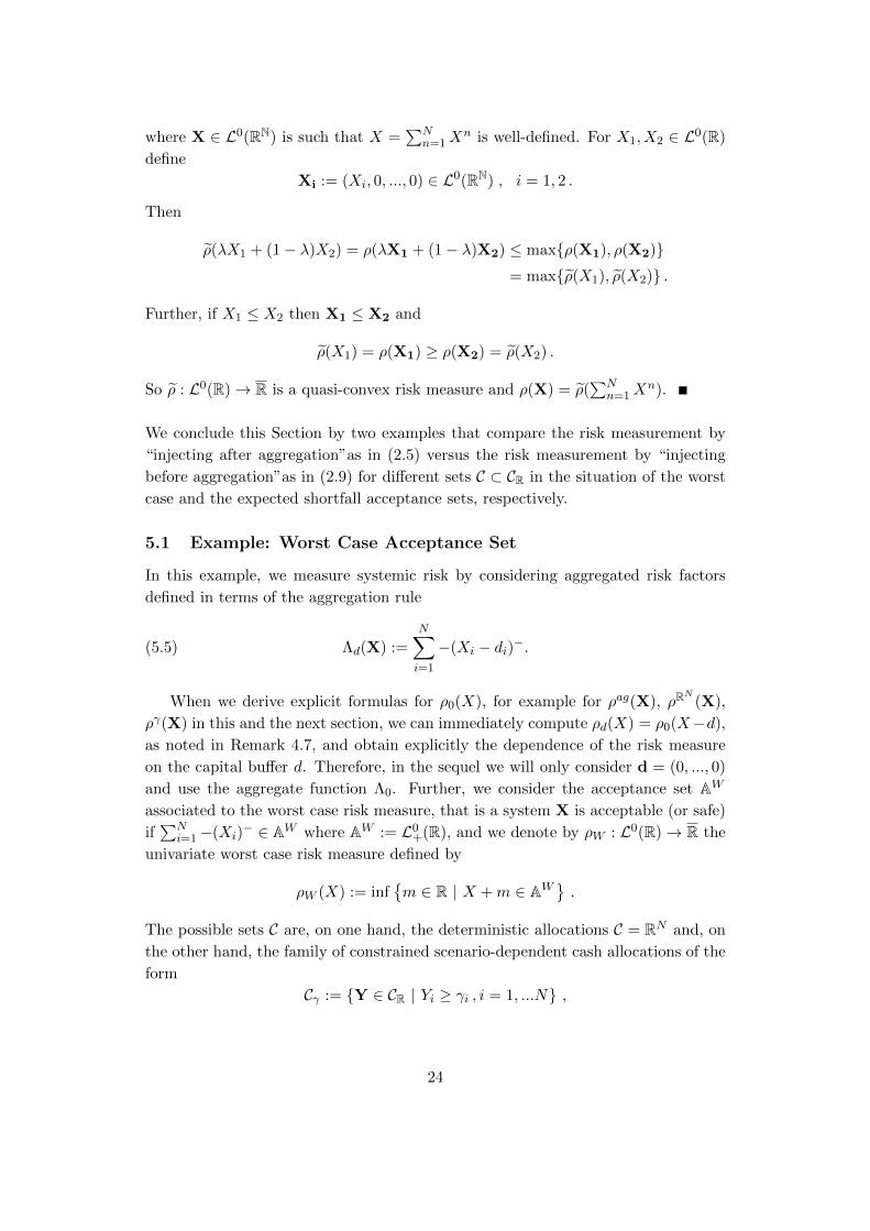
ρ(λX1 + (1− λ)X2) = ρ(λX1 + (1− λ)X2) ≤ maxρ(X1), ρ(X2)= maxρ(X1), ρ(X2) .
Further, if X1 ≤ X2 then X1 ≤ X2 and
ρ(X1) = ρ(X1) ≥ ρ(X2) = ρ(X2) .
So ρ : L0(R)→ R is a quasi-convex risk measure and ρ(X) = ρ(∑N
n=1Xn).
We conclude this Section by two examples that compare the risk measurement by
“injecting after aggregation”as in (2.5) versus the risk measurement by “injecting
before aggregation”as in (2.9) for different sets C ⊂ CR in the situation of the worst
case and the expected shortfall acceptance sets, respectively.
5.1 Example: Worst Case Acceptance Set
In this example, we measure systemic risk by considering aggregated risk factors
defined in terms of the aggregation rule
(5.5) Λd(X) :=N∑i=1
−(Xi − di)−.
When we derive explicit formulas for ρ0(X), for example for ρag(X), ρRN
(X),
ργ(X) in this and the next section, we can immediately compute ρd(X) = ρ0(X−d),
as noted in Remark 4.7, and obtain explicitly the dependence of the risk measure
on the capital buffer d. Therefore, in the sequel we will only consider d = (0, ..., 0)
and use the aggregate function Λ0. Further, we consider the acceptance set AW
associated to the worst case risk measure, that is a system X is acceptable (or safe)
if∑N
i=1−(Xi)− ∈ AW where AW := L0
+(R), and we denote by ρW : L0(R)→ R the
univariate worst case risk measure defined by
ρW (X) := infm ∈ R | X +m ∈ AW
.
The possible sets C are, on one hand, the deterministic allocations C = RN and, on
the other hand, the family of constrained scenario-dependent cash allocations of the
form
Cγ := Y ∈ CR | Yi ≥ γi , i = 1, ...N ,
24
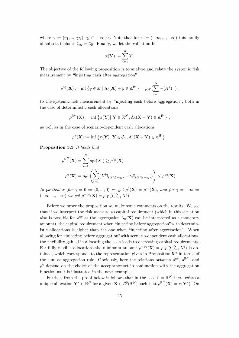
where γ := (γ1, ..., γN ), γi ∈ [−∞, 0]. Note that for γ := (−∞, ...,−∞) this family
of subsets includes C∞ = CR. Finally, we let the valuation be
π(Y) :=n∑i=1
Yi.
The objective of the following proposition is to analyze and relate the systemic risk
measurement by “injecting cash after aggregation”
ρag(X) := infy ∈ R | Λ0(X) + y ∈ AW
= ρW (
N∑i=1
−(Xi)−) ,
to the systemic risk measurement by “injecting cash before aggregation”, both in
the case of deterministic cash allocations
ρRN
(X) := infπ(Y)| Y ∈ RN ,Λ0(X + Y) ∈ AW
,
as well as in the case of scenario-dependent cash allocations
ργ(X) := infπ(Y)| Y ∈ Cγ ,Λ0(X + Y) ∈ AW
.
Proposition 5.3 It holds that
ρRN
(X) =N∑i=1
ρW (Xi) ≥ ρag(X)
ργ(X) = ρW
(N∑i=1
(XiIXi≤−γi − γiIXi≥−γi)
)≤ ρag(X) .
In particular, for γ = 0 := (0, ..., 0) we get ρ0(X) = ρag(X), and for γ = −∞ :=
(−∞, ...,−∞) we get ρ−∞(X) = ρW (∑N
i=1Xi).
Before we prove the proposition we make some comments on the results. We see
that if we interpret the risk measure as capital requirement (which in this situation
also is possible for ρag as the aggregation Λ0(X) can be interpreted as a monetary
amount), the capital requirement when “injecting before aggregation”with determin-
istic allocations is higher than the one when “injecting after aggregation”. When
allowing for “injecting before aggregation”with scenario-dependent cash allocations,
the flexibility gained in allocating the cash leads to decreasing capital requirements.
For fully flexible allocations the minimum amount ρ−∞(X) = ρW (∑N
i=1Xi) is ob-
tained, which corresponds to the representation given in Proposition 5.2 in terms of
the sum as aggregation rule. Obviously, here the relations between ρag, ρRN
, and
ργ depend on the choice of the acceptance set in conjunction with the aggregation
function as it is illustrated in the next example.
Further, from the proof below it follows that in the case C = RN there exists a
unique allocation Y∗ ∈ RN for a given X ∈ L0(RN ) such that ρRN
(X) = π(Y∗). On
25
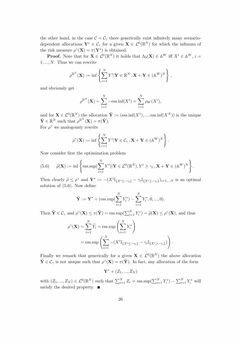
the other hand, in the case C = Cγ there generically exist infinitely many scenario-
dependent allocations Y∗ ∈ Cγ for a given X ∈ L0(RN ) for which the infimum of
the risk measure ργ(X) = π(Y∗) is obtained.
Proof. Note that for X ∈ L0(RN ) it holds that Λ0(X) ∈ AW iff Xi ∈ AW , i =
1, ..., N . Thus we can rewrite
ρRN
(X) := inf
N∑i=1
Y i|Y ∈ RN ,X + Y ∈ (AW )N
,
and obviously get
ρRN
(X) =N∑i=1
−ess.inf(Xi) =N∑i=1
ρW (Xi),
and for X ∈ L0(RN ) the allocation Y := (ess.inf(X1), ..., ess.inf(XN )) is the unique
Y ∈ RN such that ρRN
(X) = π(Y).
For ργ we analogously rewrite
ργ(X) := inf
N∑i=1
Y i|Y ∈ Cγ ,X + Y ∈ (AW )N
.
Now consider first the optimization problem
(5.6) ρ(X) := inf
ess.sup(
N∑i=1
Y i)|Y ∈ L0(RN ), Y i ≥ γi ,X + Y ∈ (AW )N
.
Then clearly ρ ≤ ργ and Y∗ := −(XiIXi≤−γi − γiIXi≥−γi)i=1,...N is an optimal
solution of (5.6). Now define
Y := Y∗ + (ess.sup(N∑i=1
Y ∗i )−N∑i=1
Y ∗i , 0, ..., 0).
Then Y ∈ Cγ and ργ(X) ≤ π(Y) = ess.sup(∑N
i=1 Y∗i ) = ρ(X) ≤ ργ(X), and thus
ργ(X) =N∑i=1
Yi = ess.sup
(N∑i=1
Y ∗i
)
= ess.sup
(N∑i=1
−(XiIXi≤−γi − γiIXi≥−γi)
).
Finally we remark that generically for a given X ∈ L0(RN ) the above allocation
Y ∈ Cγ is not unique such that ργ(X) = π(Y). In fact, any allocation of the form
Y∗ + (Z1, ..., ZN )
with (Z1, ..., ZN ) ∈ L0(RN ) such that∑N
i=1 Zi = ess.sup(∑N
i=1 Y∗i ) −
∑Ni=1 Y
∗i will
satisfy the desired property.
26
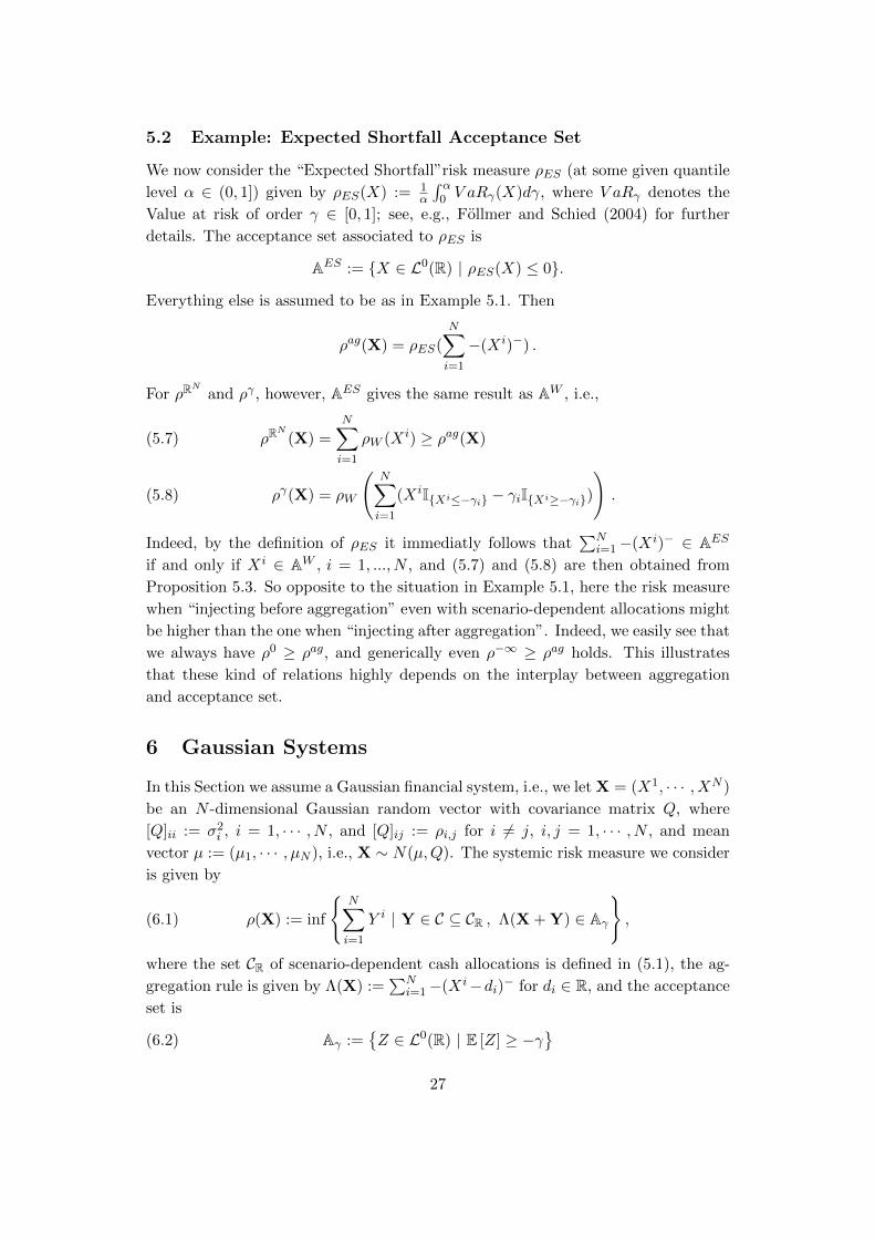
5.2 Example: Expected Shortfall Acceptance Set
We now consider the “Expected Shortfall”risk measure ρES (at some given quantile
level α ∈ (0, 1]) given by ρES(X) := 1α
∫ α0 V aRγ(X)dγ, where V aRγ denotes the
Value at risk of order γ ∈ [0, 1]; see, e.g., Follmer and Schied (2004) for further
details. The acceptance set associated to ρES is
AES := X ∈ L0(R) | ρES(X) ≤ 0.
Everything else is assumed to be as in Example 5.1. Then
ρag(X) = ρES(
N∑i=1
−(Xi)−) .
For ρRN
and ργ , however, AES gives the same result as AW , i.e.,
ρRN
(X) =N∑i=1
ρW (Xi) ≥ ρag(X)(5.7)
ργ(X) = ρW
(N∑i=1
(XiIXi≤−γi − γiIXi≥−γi)
).(5.8)
Indeed, by the definition of ρES it immediatly follows that∑N
i=1−(Xi)− ∈ AES
if and only if Xi ∈ AW , i = 1, ..., N , and (5.7) and (5.8) are then obtained from
Proposition 5.3. So opposite to the situation in Example 5.1, here the risk measure
when “injecting before aggregation” even with scenario-dependent allocations might
be higher than the one when “injecting after aggregation”. Indeed, we easily see that
we always have ρ0 ≥ ρag, and generically even ρ−∞ ≥ ρag holds. This illustrates
that these kind of relations highly depends on the interplay between aggregation
and acceptance set.
6 Gaussian Systems
In this Section we assume a Gaussian financial system, i.e., we let X = (X1, · · · , XN )
be an N -dimensional Gaussian random vector with covariance matrix Q, where
[Q]ii := σ2i , i = 1, · · · , N , and [Q]ij := ρi,j for i 6= j, i, j = 1, · · · , N , and mean
vector µ := (µ1, · · · , µN ), i.e., X ∼ N(µ,Q). The systemic risk measure we consider
is given by
(6.1) ρ(X) := inf
N∑i=1
Y i | Y ∈ C ⊆ CR , Λ(X + Y) ∈ Aγ
,
where the set CR of scenario-dependent cash allocations is defined in (5.1), the ag-
gregation rule is given by Λ(X) :=∑N
i=1−(Xi−di)− for di ∈ R, and the acceptance
set is
(6.2) Aγ :=Z ∈ L0(R) | E [Z] ≥ −γ
27
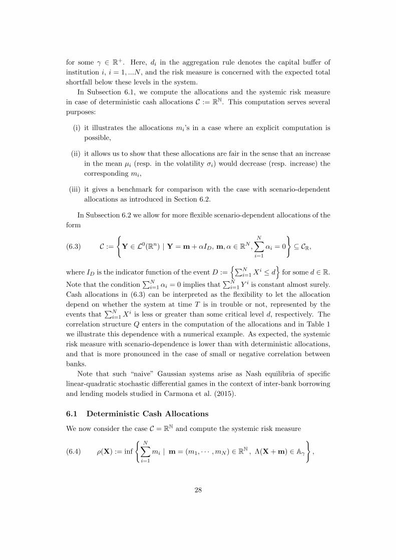
for some γ ∈ R+. Here, di in the aggregation rule denotes the capital buffer of
institution i, i = 1, ...N , and the risk measure is concerned with the expected total
shortfall below these levels in the system.
In Subsection 6.1, we compute the allocations and the systemic risk measure
in case of deterministic cash allocations C := RN. This computation serves several
purposes:
(i) it illustrates the allocations mi’s in a case where an explicit computation is
possible,
(ii) it allows us to show that these allocations are fair in the sense that an increase
in the mean µi (resp. in the volatility σi) would decrease (resp. increase) the
corresponding mi,
(iii) it gives a benchmark for comparison with the case with scenario-dependent
allocations as introduced in Section 6.2.
In Subsection 6.2 we allow for more flexible scenario-dependent allocations of the
form
(6.3) C :=
Y ∈ L0(Rn) | Y = m + αID, m, α ∈ RN ,
N∑i=1
αi = 0
⊆ CR,
where ID is the indicator function of the event D :=∑N
i=1Xi ≤ d
for some d ∈ R.
Note that the condition∑N
i=1 αi = 0 implies that∑N
i=1 Yi is constant almost surely.
Cash allocations in (6.3) can be interpreted as the flexibility to let the allocation
depend on whether the system at time T is in trouble or not, represented by the
events that∑N
i=1Xi is less or greater than some critical level d, respectively. The
correlation structure Q enters in the computation of the allocations and in Table 1
we illustrate this dependence with a numerical example. As expected, the systemic
risk measure with scenario-dependence is lower than with deterministic allocations,
and that is more pronounced in the case of small or negative correlation between
banks.
Note that such “naive” Gaussian systems arise as Nash equilibria of specific
linear-quadratic stochastic differential games in the context of inter-bank borrowing
and lending models studied in Carmona et al. (2015).
6.1 Deterministic Cash Allocations
We now consider the case C = RN and compute the systemic risk measure
(6.4) ρ(X) := inf
N∑i=1
mi | m = (m1, · · · ,mN ) ∈ RN , Λ(X + m) ∈ Aγ
,
28

where for notational clarity we write m instead of Y for deterministic cash alloca-
tions. We thus need to minimize the objective function∑N
i=1mi over RN under the
constrained Λ(X + m) ∈ Aγ , which clearly is equivalent to the constraint
(6.5)
N∑i=1
E[(Xi +mi − di)−
]= γ .
This constrained optimization problem can be solved with the associated Lagrangian
(6.6) L(m1, ...,mN , λ) :=N∑i=1
mi + λ(N∑i=1
ψi(mi)− γ)
where ψi(mi) := E[(Xi +mi − di)−
]. As Xi ∼ N(µi, σ
2i ), one obtains for i =
1, ..., N that
(6.7) ψi(mi) =σi√2π
exp
[−(di − µi −mi)
2
2σ2i
]− (mi + µi − di)Φ(
di − µi −mi
σi),
where Φ(x) =∫ x−∞
1√2πe−t
2/2dt. By direct computation this leads to
(6.8)∂L(m1, ...,mN , λ)
∂mi= 1− λΦ(
di − µi −mi
σi).
By solving the Lagrangian system we then obtain the critical point m∗ = (m∗1, · · · ,m∗N )
given by
m∗i = di − µi − σiR,
where R solves the equation
(6.9) P (R) := RΦ(R) +1√2π
exp
[−R
2
2
]=
γ∑Ni=1 σi
.
It is easily verified that m∗ is indeed a global minimum and thus the optimal cash
allocation associated with the risk measure (6.4).
We now investigate the sensitivity of the optimal solution m∗i to changes in the
underlying drift and volatility. From now on, we assume that γ∑Ni=1 σi
< P (0) = 1√2π
which ensures that R < 0. This condition is satisfied as soon as γ is small enough or
N is large enough if volatilities are uniformly bounded away from zero for instance.
In particular we obtain the following:
1.∂m∗i∂µi
= −1: the systemic riskiness decreases with increasing mean.
2.∂m∗i∂σi
> 0: the systemic riskiness increases with increasing volatility. This is
obtained as follows. We have
(6.10)∂m∗i∂σi
= −R− σi∂R
∂σi.
29

By differentiating (6.9) we obtain
(6.11)∂P
∂σi=∂P
∂R
∂R
∂σi= − γ
(∑N
k=1 σk)2.
As ∂P∂R = Φ(R), we can compute ∂R
∂σiand substitute it in (6.10)
∂m∗i∂σi
= −R+σiγ
(∑N
k=1 σk)2
1
Φ(R)
= −R+σi(∑N
k=1 σk)P (R)
(∑N
k=1 σk)2Φ(R)
= −R+σi(RΦ(R) + 1√
2πexp
[−R2
2
])
(∑N
k=1 σk)Φ(R)
= (σi∑Nk=1 σk
− 1)R+σi∑Nk=1 σk
1√2πΦ(R)
exp
[−R
2
2
].
which is positive as R < 0.
6.2 A Class of Scenario-Dependent Allocations
We now allow for different allocations of the total capital at disposal depending on
which state the system is in. More precisely, we differentiate between the two states
that D := S ≤ d and Dc = S > d for some level d ∈ R and S :=∑N
i=1Xi, and
consider allocations C given in (6.3). The systemic risk measure now becomes
ρ(X) := inf
N∑i=1
mi| m + αID ∈ C , Λ(X + m + αID) ∈ Aγ
.
To compute the risk measure in this case, we now need to minimize the objective
function∑N
i=1mi over (m, α) ∈ R2N under the constraints
N∑i=1
αi = 0 andN∑i=1
E[(Xi +mi + αiID − di)−
]= γ .
In analogy to the Section 6.1, we apply the method of Lagrange multipliers to
minimize the function
L(m1, · · · ,mN , α1, · · · , αN−1, λ) =N∑i=1
mi + λ (Ψ(m1, · · · ,mN , α1, · · · , αN−1)− γ) ,(6.12)
where
Ψ(m1, · · · ,mN , α1, · · · , αN−1) :=
N−1∑i=1
E[(Xi +mi + αiID − di)−
]+ E
(XN +mN −N−1∑j=1
αjID − dN )−
,30
as follows.
1. By computing the derivatives with respect to αi, i = 1, · · · , N − 1: ∂L∂αi
= 0 if
and only if
(6.13) Fi,S(di −mi − αi, d) = FN,S(dN −mN +
N−1∑j=1
αj , d)
for i = 1, · · · , N − 1, where Fi,S and FN,S are the joint distribution functions
of (Xi, S) and (XN , S), respectively.
2. By computing the derivatives with respect to mi, for i = 1, · · · , N−1: ∂L∂mi
= 0
if and only if
Φ(di − µi −mi
σi) + Fi,S(di −mi, d) =
Φ(dN − µn −mN
σn) + FN,S(dN −mN , d),(6.14)
for i = 1, · · · , N − 1.
3. By computing the derivatives with respect to λ: we have ∂L∂λ = 0 if and only if
Ψ(m1, · · · ,mN , α1, · · · , αN−1) = γ, where
Ψ(m1, · · · ,mN , α1, · · · , αN−1) =
N∑i=1
ψi(mi)
+N−1∑i=1
[(mi − di)FN,S(di −mi, d)− (mi + αi − di)Fi,S(di −mi − αi, d)
+
∫ di−mi
di−mi−αi
∫ d
−∞xFi,S(x, y)dydx
]+ (mN − dN )FN,S(dN −mN , d)
− (mN −N−1∑j=1
αj − dN )FN,S(dN −mN +N−1∑j=1
αj , d)
+
∫ dN−mN
dN−mN+∑N−1
j=1 αj
∫ d
−∞xFN,S(x, y)dydx,
and ψi, i = 1, · · · , N , are defined in (6.7).
From (6.12) and (6.13) we immediately obtain that if the Xi, i = 1, · · · , N , are iden-
tically distributed, then the optimal solution is obtained for αi = 0, i = 1, · · · , N ,
and corresponds to the one obtained explicitly in Section 6.1 for deterministic injec-
tions.
We now present numerical illustrations of our results in the simple case with two
banks. In Table 1 we set the means µi = 0 for i = 1, 2, the standard deviations
31
ρ1,2 ↓ Deterministic Random
m1 0.5772 0.1597
m2 1.7316 1.7230
-0.8 α 0 2.8704
ρ = m1 +m2 2.3088 1.8827
m1 0.5772 0.2908
m2 1.7316 1.7776
-0.5 α 0 2.3161
ρ = m1 +m2 2.3088 2.0683
m1 0.5772 0.4490
m2 1.7316 1.7796
0 α 0 1.7208
ρ = m1 +m2 2.3088 2.2286
m1 0.5772 0.5463
m2 1.7316 1.7461
0.5 α 0 1.3389
ρ = m1 +m2 2.3088 2.2924
m1 0.5772 0.5737
m2 1.7316 1.7314
0.8 α 0 0.7905
ρ = m1 +m2 2.3088 2.3053
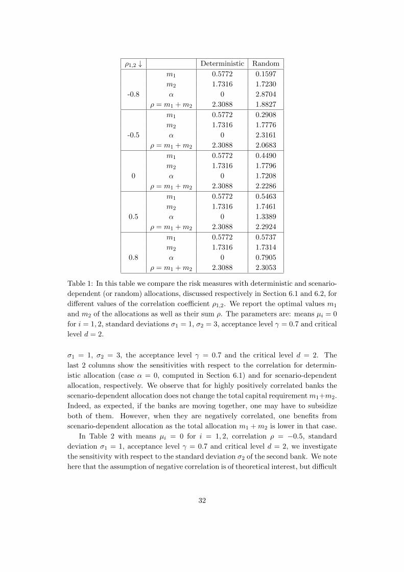
Table 1: In this table we compare the risk measures with deterministic and scenario-
dependent (or random) allocations, discussed respectively in Section 6.1 and 6.2, for
different values of the correlation coefficient ρ1,2. We report the optimal values m1
and m2 of the allocations as well as their sum ρ. The parameters are: means µi = 0
for i = 1, 2, standard deviations σ1 = 1, σ2 = 3, acceptance level γ = 0.7 and critical
level d = 2.
σ1 = 1, σ2 = 3, the acceptance level γ = 0.7 and the critical level d = 2. The
last 2 columns show the sensitivities with respect to the correlation for determin-
istic allocation (case α = 0, computed in Section 6.1) and for scenario-dependent
allocation, respectively. We observe that for highly positively correlated banks the
scenario-dependent allocation does not change the total capital requirement m1+m2.
Indeed, as expected, if the banks are moving together, one may have to subsidize
both of them. However, when they are negatively correlated, one benefits from
scenario-dependent allocation as the total allocation m1 +m2 is lower in that case.
In Table 2 with means µi = 0 for i = 1, 2, correlation ρ = −0.5, standard
deviation σ1 = 1, acceptance level γ = 0.7 and critical level d = 2, we investigate
the sensitivity with respect to the standard deviation σ2 of the second bank. We note
here that the assumption of negative correlation is of theoretical interest, but difficult
32
σ2 ↓ Deterministic Random
m1 0.1008 0.1008
m2 0.1031 0.1031
1 α 0 0.0002
ρ = m1 +m2 0.2039 0.2039
m1 0.8168 0.3167
m2 4.0816 4.1295
5 α 0 3.5987
ρ = m1 +m2 4.8984 4.4462
m1 1.1417 0.4631
m2 11.3964 11.4333
10 α 0 6.9909
ρ = m1 +m2 12.5381 11.8963
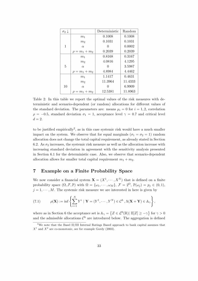
Table 2: In this table we report the optimal values of the risk measures with de-
terministic and scenario-dependent (or random) allocations for different values of
the standard deviation. The parameters are: means µi = 0 for i = 1, 2, correlation
ρ = −0.5, standard deviation σ1 = 1, acceptance level γ = 0.7 and critical level
d = 2.
to be justified empirically2, as in this case systemic risk would have a much smaller
impact on the system. We observe that for equal marginals (σ1 = σ2 = 1) random
allocation does not change the total capital requirement, as already stated in Section
6.2. As σ2 increases, the systemic risk measure as well as the allocation increase with
increasing standard deviation in agreement with the sensitivity analysis presented
in Section 6.1 for the deterministic case. Also, we observe that scenario-dependent
allocation allows for smaller total capital requirement m1 +m2.
7 Example on a Finite Probability Space
We now consider a financial system X = (X1, · · · , XN ) that is defined on a finite
probability space (Ω,F ,P) with Ω = ω1, · · · , ωM, F = 2Ω, P(ωj) = pj ∈ (0, 1),
j = 1, · · · ,M . The systemic risk measure we are interested in here is given by
(7.1) ρ(X) := inf
N∑i=1
Y i | Y = (Y 1, · · · , Y N ) ∈ Ch ,Λ(X + Y) ∈ Aγ
,
where as in Section 6 the acceptance set is Aγ =Z ∈ L0(R)| E[Z] ≥ −γ
for γ > 0
and the admissible allocations Ch are introduced below. The aggregation is defined
2We note that the Basel II/III Internal Ratings Based approach to bank capital assumes that
X1 and X2 are co-monotonic, see for example Gordy (2003).
33
by
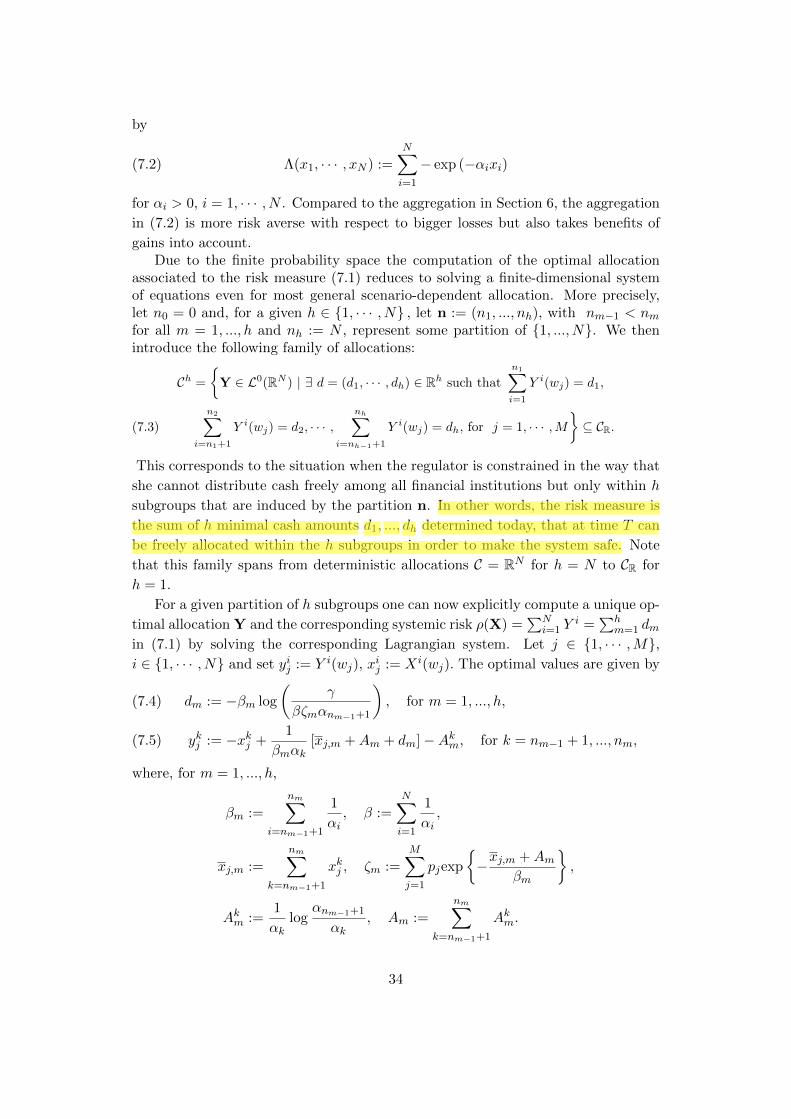
(7.2) Λ(x1, · · · , xN ) :=
N∑i=1
− exp (−αixi)
for αi > 0, i = 1, · · · , N . Compared to the aggregation in Section 6, the aggregation
in (7.2) is more risk averse with respect to bigger losses but also takes benefits of
gains into account.Due to the finite probability space the computation of the optimal allocation
associated to the risk measure (7.1) reduces to solving a finite-dimensional systemof equations even for most general scenario-dependent allocation. More precisely,let n0 = 0 and, for a given h ∈ 1, · · · , N , let n := (n1, ..., nh), with nm−1 < nmfor all m = 1, ..., h and nh := N , represent some partition of 1, ..., N. We thenintroduce the following family of allocations:
Ch =
Y ∈ L0(RN ) | ∃ d = (d1, · · · , dh) ∈ Rh such that
n1∑i=1
Y i(wj) = d1,
n2∑i=n1+1
Y i(wj) = d2, · · · ,nh∑
i=nh−1+1
Y i(wj) = dh, for j = 1, · · · ,M⊆ CR.(7.3)
This corresponds to the situation when the regulator is constrained in the way that
she cannot distribute cash freely among all financial institutions but only within h
subgroups that are induced by the partition n. In other words, the risk measure is
the sum of h minimal cash amounts d1, ..., dh determined today, that at time T can
be freely allocated within the h subgroups in order to make the system safe. Note
that this family spans from deterministic allocations C = RN for h = N to CR for
h = 1.
For a given partition of h subgroups one can now explicitly compute a unique op-
timal allocation Y and the corresponding systemic risk ρ(X) =∑N
i=1 Yi =
∑hm=1 dm
in (7.1) by solving the corresponding Lagrangian system. Let j ∈ 1, · · · ,M,i ∈ 1, · · · , N and set yij := Y i(wj), x
ij := Xi(wj). The optimal values are given by
dm := −βm log
(γ
βζmαnm−1+1
), for m = 1, ..., h,(7.4)
ykj := −xkj +1
βmαk[xj,m +Am + dm]−Akm, for k = nm−1 + 1, ..., nm,(7.5)
where, for m = 1, ..., h,
βm :=
nm∑i=nm−1+1
1
αi, β :=
N∑i=1
1
αi,
xj,m :=
nm∑k=nm−1+1
xkj , ζm :=
M∑j=1
pjexp
−xj,m +Am
βm
,
Akm :=1
αklog
αnm−1+1
αk, Am :=
nm∑k=nm−1+1
Akm.
34

The proof rely on a straightforward but tedious verification that the formulas (7.4)and (7.5) are the solutions of the system ∇L = 0, where the Lagrangian is given by
L(d1, ..., dh, (ykj )j,k, λ, δ) = d+λ
M∑j=1
pj
h∑m=1
nm∑k=nm−1+1
e−αk(xkj+y
kj ) − γ
+δ
(N∑i=1
Y i − d
),
with λ = βγ and d =
∑hm=1 dm.
The value of the risk measure ρ(X) explicitly depends on the values αi > 0,
i = 1, · · · , N, on the parameter γ, on the probability P and on xij , i = 1, · · · , N,j = 1, · · · ,M. These computations are useful to compare the risk measure ρN (X)
with deterministic allocations (h = N) with the the risk measure ρ1(X) with fully
unconstrained scenario-dependent allocations (h = 1). The difference ρN (X) −ρ1(X) represents the potential amount that can be saved by adopting the scenario-
dependent allocations that we propose in this paper, in contrast to the standard
practice of deterministic allotments. In addition, with the above formulas we can
show that the risk measure with scenario-dependent allocations is very sensible to
the dependence structure of the components of the vector X = (X1, · · · , XN ), even
though the set Aγ of acceptable positions is defined via the marginal distributions of
Xi, i = 1, · · · , N, only. This fact is pointed out in the next simple example, where we
compare the values of the risk measures ρ(X) for the six possible different choices of
grouping four given banks X1, · · · , X4 into three subgroups (h = 3), as for exampleX1,X2, X3
,X4
. The outcome strongly depends on whether the two banks
that we group together are independent, comonotone or countermonotone.
Example 7.1 We consider a system of four banks represented by the random vari-
ables X1, X2, X3 and X4 on the probability space (Ω,F ,P), where Ω = (ω1, ω2, ω3, ω4),
F = 2Ω and P(ω1) = 0.64, P(ω2) = P(ω3) = 0.16 and P(ω4) = 0.04. We assume
that X4 is independent of X1, X2, X3, that X2 is comonotone with X1 and that
X3 is countermonotone with X1. Furthermore X1(w1) = X1(w3) = 100, X1(w2) =
X1(w4) = −50, X2(w1) = X2(w3) = 50, X2(w2) = X2(w4) = −25, X3(w1) =
X3(w3) = −25, X3(w2) = X3(w4) = 50 and X4(w1) = X4(w2) = 50, X4(w3) =
X4(w4) = −25. We set αi = 0.3 for i = 1, · · · , 4 and γ = 50 and consider the
set Ch defined above. Note that here ρ(0) is not zero, but it could be normalized by
replacing ρ(·) with ρ(·)− ρ(0).
In Table 3 we provide the systemic risk measures when the number of subgroups
is h = 1 or h = 2 or h = 3 or h = 4. From Table 3 we note that the maximum and
minimum value of ρ are obtained respectively in the deterministic (h = 4) and the
fully unconstrained scenario-dependent (h = 1) cases.
For h = 3, we always have three groups, where two are singleton and one is
composed of two banks (which are shown in the table). In this cases, whenever
one groups X1 and X3, or X2 and X3, ρ is substantially reduced (−0.56 or 4.44),
compared to the deterministic case (79.02), as these couples of vectors are counter
monotone; whenever one groups X4 with any of the X1, X2, X3, there is little
35

Syst. risk
measure
Case Syst. risk
measure
Case
−26.36 h = 1
−0.56 h = 3, X1, X3 −15.86 h = 2, X1, X3, X2, X44.44 h = 3, X2, X3 −5.13 h = 2, X2, X3, X1, X463.71 h = 3, X2, X468.36 h = 3, X1, X472.96 h = 3, X3, X4 68.37 h = 2, X3, X4, X1, X274.48 h = 3, X1, X279.02 h = 4
Table 3: In this table we report the values of the systemic risk measure (first and
third columns) for different grouping of the four banks of the Example 7.1. The cases
h = 1 and h = 4 correspond respectively to one large group and to the 4 individual
banks. In the case h = 3 there are three groups, two of which consist of a single
bank and the third one is composed of the two banks showed in the second column.
For h = 2 the two groups are shown in the fourth column and the corresponding
risk measure in the third one.
difference (68.36, 63.71, 72.96) with respect to the deterministic case (79.02), as X4
is independent from the others; grouping X1 and X2 has very little effect (74.48)
compared to the deterministic case (79.02), as X1 and X2 are comonotone.
For h = 2, we have two groups each one with two banks. We always obtain a
reduction of ρ when compared to grouping the same two banks but leaving the other
two as singleton (compare the cases h = 3 and h = 2 on the same line). As expected,
the size of the reduction is associated to the dependence structure of the component
of X.
Remark 7.2 One could extend the above setting further by considering the possi-
bility to limit cross-subsidization in the allocations. This can be done by adding
the constraint Y i ≥ bi, i = 1, · · · , N into the family (7.3) of cash allocations, where
(b1, ..., bN ) ∈ RN . For example, putting b := (0, ..., 0) excludes cash withdrawals from
institutions and in this sense doesn’t allow for any cross-subsidization. The systemic
risk measure and corresponding optimal allocations solution can now be computed by
resorting to the Karush Kuhn Tucker conditions (Boyd and Vandenberghe (2009)),
see the computations in Pastore (2014).
7.1 Allocating systemic risk shares
In this subsection, we propose to determine an allocation of systemic risk by comput-
ing the expectations EQ[Y i], i = 1, ..., N , of the scenario-dependent cash allocations
in (7.5). When the probability measure Q is appropriately selected, such allocation
36

has some nice fairness properties that are illustrated below in (7.10), (7.11) and
(7.12).
To ease notation, we consider the case of one single group (h = 1) and we assume
that αi = α for some α > 0, i = 1, ..., N , but the analysis can be generalized to any
other grouping and heterogeneous αi. Then (7.5) reduces to
(7.6) yij :=
[xjN− xij
]+
d
N, i = 1, ..., N ,
where yij := Y i(ωj), xij := Xi(ωj), xj :=
∑Ni=1 x
ij and
(7.7) d := ρ(X) =N
αlog
(N
γE
[exp
(−αX
N
)])with X :=
∑Ni=1X
i. The term d/N in (7.6) represents the scenario-independent
part of allocation yij , while the first parenthesis can be interpreted as some scenario-
dependent mean-field term which increases or decreases allocation yij according to
how much the individual risk xij is below or above the group average xj/N .
Let Q be a probability measure and let Y i ∈ L0(R) be the scenario-dependent
cash allocations given in (7.6). We may define the systemic risk share of bank i by
the real number EQ[Y i]. Then, for each Q, (EQ[Y i])i=1,...,N , constitutes an allocation
of the total systemic risk
N∑i=1
EQ[Y i] = EQ
[N∑i=1
Y i
]= EQ[ρ(X)] = ρ(X).
Now let us consider a change in the vector X by adding another vector εZ, for
some ε ∈ R and Z = (Z1, ..., ZN ) ∈ L0(RN ). We put Xi,ε := Xi + εZi, i = 1, ..., N ,
and Xε := (X1,ε, ..., XN,ε). We then compare the optimal solutions yij(X+εZ), given
in equation (7.6), with yij(X) and the risk measure ρ(X+εZ) with ρ(X), respectively.
(i) We first consider the situation in which the institutions add some cash
amounts to their positions, i.e., we set Z = c = (c1, ..., cN ) ∈ RN and ε = 1. A
straightforward computation then gives the following cash invariance of both the
risk measure ρ (see also (2.14)) and the components yij for all i = 1, .., N and
j = 1, ...,M
(7.8) ρ(X + c) = ρ(X)−N∑i=1
ci, yij(X + c) = yij(X)− ci, c ∈ RN .
In particular, if only institution l ∈ 1, ..., N changes its position by a cash amount,
i.e., ci = 0 for i 6= l, the change ρ(X + c)− ρ(X) = −cl in total systemic risk is ex-
actly covered by the change in the risk allocation EQ[Y l(X + c)]−EQ[Y l(X)] = −cl
of institution l, whereas the risk allocations of the other institutions are unchanged:
EQ[Y i(X + c)] − EQ[Y i(X)] = 0 for i 6= l (whatever Q might be). This full re-
sponsibility for one’s own changes in the financial position is an allocation property
37
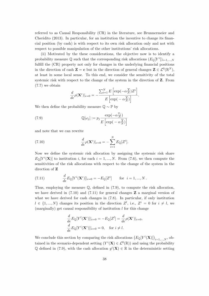
referred to as Causal Responsibility (CR) in the literature, see Brunnermeier and
Cheridito (2013). In particular, for an institution the incentive to change its finan-
cial position (by cash) is with respect to its own risk allocation only and not with
respect to possible manipulation of the other institutions’ risk allocations.
(ii) Motivated by the these considerations, the objective now is to identify a
probability measure Q such that the corresponding risk allocations (EQ[Y i])i=1,...,N
fulfill the (CR) property not only for changes in the underlying financial positions
in the direction of cash Z = c but in the direction of general changes Z ∈ L0(RN ),
at least in some local sense. To this end, we consider the sensitivity of the total
systemic risk with respect to the change of the system in the direction of Z. From
(7.7) we obtain
d
dερ(Xε)|ε=0 = −
∑Ni=1E
[exp(−αXN )Zi
]E[exp(− αXN )
] .
We then define the probability measure Q ∼ P by
(7.9) Q[ωj ] := pjexp(−αxjN )
E[exp(− αXN )
]and note that we can rewrite
(7.10)d
dερ(Xε)|ε=0 = −
N∑i=1
EQ[Zi].
Now we define the systemic risk allocation by assigning the systemic risk share
EQ[Y i(X)] to institution i, for each i = 1, ..., N . From (7.6), we then compute the
sensitivities of the risk allocations with respect to the change of the system in the
direction of Z
(7.11)d
dεEQ[Y i(Xε)]|ε=0 = −EQ[Zi] for i = 1, ..., N .
Thus, employing the measure Q, defined in (7.9), to compute the risk allocation,
we have derived in (7.10) and (7.11) for general changes Z a marginal version of
what we have derived for cash changes in (7.8). In particular, if only institution
l ∈ 1, ..., N changes its position in the direction Z l, i.e., Zi = 0 for i 6= l, we
(marginally) get causal responsibility of institution l for this change
d
dεEQ[Y l(Xε)]|ε=0 = −EQ[Z l] =
d
dερ(Xε)|ε=0,
d
dεEQ[Y i(Xε)]|ε=0 = 0, for i 6= l.
We conclude this section by comparing the risk allocations(EQ[Y i(X)]
)i=1,...,N
, ob-
tained in the scenario-dependent setting (Y i(X) ∈ L0(R)) and using the probability
Q defined in (7.9), with the cash allocation yi(X) ∈ R in the deterministic setting
38

(h = N), which is now interpreted as risk allocation to institution i. It is easily ver-
ified from (7.5), taking h = N , that the deterministic risk allocation of institution
i is given by yi(X) = 1α log
(Nγ EP
[e−αX
i])
. We also know that when going from
deterministic to scenario-dependent allocations the total systemic risk decreases. It
is then desirable that each institution profits from this decrease in total systemic
risk in the sense that also its individual risk share decreases
(7.12) EQ[Y i(X)] ≤ yi(X), for each i = 1, ..., N.
The opposite would clearly be perceived as unfair. The following computation shows
that our allocation fulfills this property. Indeed, from (7.6) and (7.7), Jensen’s
inequality, and (7.9) we obtain
EQ[Y i(X)] = EQ
[X
N−Xi
]+
1
αlog
(N
γEP
[e−α
XN
])=
1
αlog exp
αEQ
[X
N−Xi
]+
1
αlog
(N
γEP
[e−α
XN
])≤ 1
αlog
EQ
[eα(
XN−Xi
)]+
1
αlog
(N
γEP
[e−α
XN
])=
1
αlog
(N
γEP
[e−αX
i])
= yi(X).
A Appendix
A.1 Gaussian Case with Random Injections
We provide here the computations necessary to minimize the function (6.12). We
first consider
E[(Xi + Y i − di)−
]= E
[(Xi +mi + αiID − di)−
]= E
[(Xi +mi + αi − di)−ID
]+ E
[(Xi +mi − di)−IAc
]= E
[(Xi +mi + αi − di)− − (Xi +mi − di)−
ID]
+ E[(Xi +mi − di)−
](A.1)
for i = 1, · · · , N . To compute (A.1), we distinguish between the cases αi > 0
and αi < 0. Note that by the definition of C, we cannot a priori argue on the
sign of α. For αi > 0, we have thatXi ≤ di −mi
=Xi ≤ di −mi − αi
∪
di −mi − αi < Xi ≤ di −mi
. Here we set A1 :=
Xi ≤ di −mi − αi
and A2 :=
di −mi − αi < Xi ≤ di −mi
. Then
(Xi +mi + αi − di)− − (Xi +mi − di)− = −αiIA1 + (Xi +mi − di)IA2 ,
39

and
E[(Xi + Y i − di)−
]= −αiE [IA1ID] + E
[(Xi +mi − di)IA2ID
]+ E
[(Xi +mi − di)−
]= (mi − di)Fi,S(di −mi, d)− (mi + αi − di)Fi,S(di −mi − αi, d)
+
∫ di−mi
di−mi−αi
∫ d
−∞xfi,S(x, y)dydx+ E
[(Xi +mi − di)−
],
where Fi,S and fi,S are the joint distribution function and the density of (Xi, S),
respectively. Recall that in our setting (Xi, S) ∼ N2(µi, Qi) with mean vector
µi = (µi,∑n
j=1 µj) and covariance matrix
Qi =
σ2i σ2
i +∑
j 6=i ρi,jσ2i +
∑j 6=i ρi,j
∑nj=1 σ
2j +
∑nj,k=1 ρj,k
.
Analogous computations hold in the case αi < 0. Summing up, we obtain that
E
[N∑i=1
(Xi + Y i − di)−]
=N∑i=1
E[(Xi + Y i − di)−
]=
N∑i=1
E[(Xi +mi − di)−
]+
N∑i=1
Iαi≥0 [(mi − di)Fi,S(di −mi, d)− (mi + αi − di)Fi,S(di −mi − αi, d)
+
∫ di−mi
di−mi−αi
∫ d
−∞xfi,S(x, y)dydx
]+
N∑i=1
Iαi<0 [(mi − di)Fi,S(di −mi, d)− (mi + αi − di)Fi,S(di −mi − αi, d)
+
∫ di−mi
di−mi−αi
∫ d
−∞xfi,S(x, y)dydx
]
40
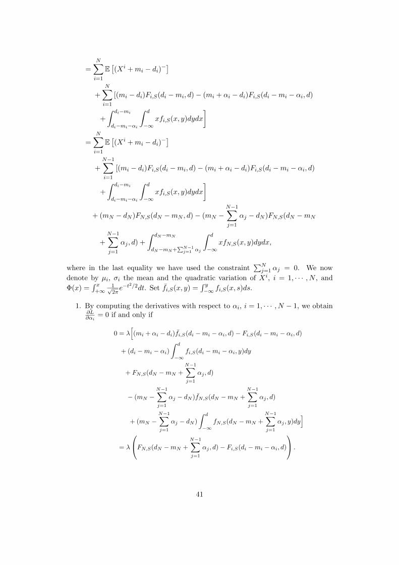
=
N∑i=1
E[(Xi +mi − di)−
]+
N∑i=1
[(mi − di)Fi,S(di −mi, d)− (mi + αi − di)Fi,S(di −mi − αi, d)
+
∫ di−mi
di−mi−αi
∫ d
−∞xfi,S(x, y)dydx
]=
N∑i=1
E[(Xi +mi − di)−
]+N−1∑i=1
[(mi − di)Fi,S(di −mi, d)− (mi + αi − di)Fi,S(di −mi − αi, d)
+
∫ di−mi
di−mi−αi
∫ d
−∞xfi,S(x, y)dydx
]+ (mN − dN )FN,S(dN −mN , d)− (mN −
N−1∑j=1
αj − dN )FN,S(dN −mN
+N−1∑j=1
αj , d) +
∫ dN−mN
dN−mN+∑N−1
j=1 αj
∫ d
−∞xfN,S(x, y)dydx,
where in the last equality we have used the constraint∑N
j=1 αj = 0. We now
denote by µi, σi the mean and the quadratic variation of Xi, i = 1, · · · , N , and
Φ(x) =∫ x
+∞1√2πe−t
2/2dt. Set fi,S(x, y) =∫ y−∞ fi,S(x, s)ds.
1. By computing the derivatives with respect to αi, i = 1, · · · , N − 1, we obtain∂L∂αi
= 0 if and only if
0 = λ[(mi + αi − di)fi,S(di −mi − αi, d)− Fi,S(di −mi − αi, d)
+ (di −mi − αi)∫ d
−∞fi,S(di −mi − αi, y)dy
+ FN,S(dN −mN +
N−1∑j=1
αj , d)
− (mN −N−1∑j=1
αj − dN )fN,S(dN −mN +
N−1∑j=1
αj , d)
+ (mN −N−1∑j=1
αj − dN )
∫ d
−∞fN,S(dN −mN +
N−1∑j=1
αj , y)dy]
= λ
FN,S(dN −mN +
N−1∑j=1
αj , d)− Fi,S(di −mi − αi, d)
.
41

We then obtain that the equation above has a solution if λ = 0 or when
(A.2) Fi,S(di −mi − αi, d) = FN,S(dN −mN +N−1∑j=1
αj , d)
for i = 1, · · · , N − 1.
2. By computing the derivatives with respect to mi, for i = 1, · · · , N , we obtain∂L∂mi
= 0 if and only if
0 = 1 + λ
(Φ(di − µi −mi
σi)− (mi − di)fi,S(di −mi, d) + Fi,S(di −mi, d)
−Fi,S(di −mi − αi, d) + (mi + αi − di)fi,S(di −mi − αi, d)
+(di −mi − αi)∫ d
−∞fi,S(di −mi − αi, y)− (di −mi)
∫ d
−∞fi,S(di −mi, y)dy
)
= 1 + λ
Φ(di − µi −mi
σi) + Fi,S(di −mi, d)− FN,S(dN −mN +
N−1∑j=1
αj , d)
,
where we have used (6.8), (A.2) and the notation above. In particular(A.3)
λ = −
Φ(dN − µN −mN
σN) + FN,S(dN −mN , d)− FN,S(dN −mN +
N−1∑j=1
αj , d)
−1 ,if the denominator is different from zero. By (A.3) we then obtain
Φ(di − µi −mi
σi) + Fi,S(di −mi, d)
= Φ(dN − µN −mN
σN) + FN,S(dN −mN , d),(A.4)
for i = 1, · · · , N − 1.
References
Acharya, V., Pedersen, L., Philippon, T., and Richardson, M. (2010). Measuring
systemic risk. Working paper, New York University, Stern School of Business.
Adrian, T. and Brunnermeier, M. K. (2011). Covar. Technical report, National
Bureau of Economic Research.
Amini, H., Cont, R., and Minca, A. (2013). Resilience to contagion in financial
networks. Mathematical Finance, pages n/a–n/a.
Amini, H., Filipovic, D., and Minca, A. (2014). Systemic Risk with Central Coun-
terparty Clearing. Working paper.
42

Artzner, P., Delbaen, F., Eber, J. M., and Heath, D. (1999). Coherent measures of
risk. Math. Finance, 4:203–228.
Awiszus, K. and Weber, S. (2015). The joint impact of bankruptcy costs, cross-
holdings and fire sales on systemic risk in financial networks. Preprint.
Battiston, S. and Caldarelli, G. (2013). Systemic Risk in Financial Networks. Journal
of Financial Management Markets and Institutions, 1(2):129–154.
Battiston, S., Delli Gatti, D., Gallegati, M., Greenwald, B., and Stiglitz, J. E. (2012).
Liaisons Dangereuses: Increasing Connectivity, Risk Sharing, and Systemic Risk.
Journal of Economic Dynamics and Control, 36(8):1121–1141.
Benoit, S., Colliard, J.-E., Hurlin, C., and Perignon, C. (2016). Where the risks lie:
A survey on systemic risk. Review of Finance, forthcoming.
Black, L., Correa, R., Huang, X., and Zhou, H. (2016). The systemic risk of european
banks during the financial and sovereign debt crises. Journal of Banking and
Finance, 63:1–146.
Boss, M., Elsinger, H., Summer, M., and Thurner, S. (2004). Network topology of
the interbank market. Quantitative Finance, 4(6):677–684.
Boyd, S. and Vandenberghe, L. (2009). Convex Optimization. Cambridge University
Press.
Brunnermeier, M. K. and Cheridito, P. (2013). Measuring and allocating systemic
risk. Preprint.
Caccioli, F., Shrestha, M., Moore, C., and Farmer, J. D. (2012). Stability anal-
ysis of financial contagion due to overlapping portfolios. Preprint, available at
arXiv:1210.5987v1 [q-fin.GN].
Carmona, R., Fouque, J.-P., and Sun, L.-H. (2015). Mean field games and systemic
risk. Communications in Mathematical Sciences, 13(4):911–933.
Cerreia-Vioglio, S., Maccheroni, F., Marinacci, M., and Montrucchio, L. (2010). Risk
measures: rationality and diversification. Mathematical Finance, 21:743–774.
Chen, C., Iyengar, G., and Moallemi, C. (2013). An axiomatic approach to systemic
risk. Management Science, 59(6):1373–1388.
Cherny, A. and Madan, D. (2009). New measures for performance evaluation. Rev.
Financ. Stud., 22:2571– 2606.
Cifuentes, R., Ferrucci, G., and Shin, H. S. (2005). Liquidity risk and contagion.
Journal of the European Economic Association, 3(2-3):556–566.
43

Cont, R., Moussa, A., and Santos, E. (2013). Network structure and systemic risk
in banking systems. In Fouque, J.-P. and Langsam, J., editors, Handbook on
Systemic Risk. Cambridge.
Craig, B. and von Peter, G. (2014). Interbank tiering and money center banks.
Journal of Financial Intermediation, pages –.
Detering, N., Meyer-Brandis, T., and Panagiotou, K. (2016a). Bootstrap percolation
in directed and inhomogeneous random graphs. Preprint, University of Munich.
Detering, N., Meyer-Brandis, T., Panagiotou, K., and Ritter, D. (2016b). Manag-
ing systemic risk in inhomogeneous financial networks. Preprint, University of
Munich.
Eisenberg, L. and Noe, T. H. (2001). Systemic risk in financial systems. Management
Science, 47(2):236–249.
Feinstein, Z., Rudloff, B., and Weber, S. (2015). Measures of systemic risk. Working
paper.
Follmer, H. and Schied, A. (2002). Convex measures of risk and trading constraints.
Finance and Stochastics, 6:429–447.
Follmer, H. and Schied, A. (2004). Stochastic Finance. An introduction in discrete
time. De Gruyter, Berlin - New York.
Fouque, J.-P. and Ichiba, T. (2013). Stability in a Model of Interbank Lending.
SIAM Journal on Financial Mathematics, 4(1):784–803.
Fouque, J.-P. and Langsam, J. A., editors (2013). Handbook on Systemic Risk.
Cambridge.
Fouque, J.-P. and Sun, L.-H. (2013). Systemic risk illustrated. In Fouque, J.-P. and
Langsam, J., editors, Handbook on Systemic Risk. Cambridge.
Frittelli, M. and Maggis, M. (2014). Complete duality for quasiconvex dynamic risk
measures on modules of the lp-type. Statistics and Risk Modeling, 31(1):103–128.
Frittelli, M. and Rosazza Gianin, E. (2002). Putting order in risk measures. J. Bank.
Finance, 26:1473–1486.
Frittelli, M. and Scandolo, G. (2006). Risk measures and capital requirements for
processes. Mathematical Finance, 16(4):589–613.
Gai, P. and Kapadia, S. (2010a). Contagion in financial networks. Bank of England
Working Papers 383, Bank of England.
Gai, P. and Kapadia, S. (2010b). Liquidity hoarding, network externalities, and
interbank market collapse. Proc. R. Soc. A, 466:2401–2423.
44

Gleeson, J. P., Hurd, T. R., Melnik, S., and Hackett, A. (2013). Systemic Risk
in Banking Networks Without Monte Carlo Simulation. In Kranakis, E., editor,
Advances in Network Analysis and its Applications, volume 18 of Mathematics in
Industry, pages 27–56. Springer Berlin Heidelberg.
Gordy, M. B. (2003). A risk-factor model foundation for ratings-based bank capital
rules. Journal of Financial Intermediation, 12(3):199–232.
Hoffmann, H., Meyer-Brandis, T., and Svindland, G. (2015a). Risk-consistent con-
ditional systemic risk measures. accepted on Stochastic Processes and their Ap-
plications.
Hoffmann, H., Meyer-Brandis, T., and Svindland, G. (2015b). Strongly consistent
multivariate conditional risk measures. Preprint.
Huang, X., Zhou, H., and Zhu, H. (2009). A framework for assessing the systemic
risk of major financial institutions. Journal of Banking & Finance, 33(11):2036–
2049.
Hurd, T. R. (2016). Contagion! Systemic Risk in Financial Networks. Springer, to
appear.
Hurd, T. R., Cellai, D., Melnik, S., and Shao, Q. (2014). Illiquidity and in-
solvency: a double cascade model of financial crises. Preprint, available at
arxiv.org/pdf/1310.6873.
Kley, O., Kluppelberg, C., and Reichel, L. (2015). Systemic risk through contagion
in a core-periphery structured banking network. In A. Palczewski and L. Stettner:
Advances in Mathematics of Finance, volume 104. Banach Center Publications,
Warschau, Polen.
Kromer, E., Overbeck, L., and Zilch, K. A. (2013). Systemic risk measures on general
probability spaces. Preprint, University of Gießen, Germany.
Lee, S. H. (2013). Systemic liquidity shortages and interbank network structures.
Preprint, availble at https://ideas.repec.org/a/eee/finsta/v9y2013i1p1-12.html.
Lehar, A. (2005). Measuring systemic risk: A risk management approach. Journal
of Banking & Finance, 29(10):2577–2603.
Pastore, M. C. (2014). Systemic risk measures. Master Thesis, University of Munich.
Rogers, L. C. G. and Veraart, L. A. M. (2013). Failure and Rescue in an Interbank
Network. Management Science, 59(4):882–898.
45