a type-theoretic framework for software component
TRANSCRIPT

A Type-Theoretic Framework for Software ComponentSynthesis
Dissertation
zur Erlangung des Grades eines
D o k t o r s d e r N a t u r w i s s e n s c h a f t e n
der Technischen Universitat Dortmundan der Fakultat fur Informatik
von
Jan Bessai
Dortmund
2019

Tag der mundlichen Prufung: 29. Oktober 2019Dekan: Prof. Dr.-Ing. Gernot FinkGutachter:
Prof. Dr. Jakob Rehof (Technische Universitat Dortmund, Deutschland)Prof. Dr. George T. Heineman (Worcester Polytechnic Institute, USA)

Acknowledgments
First, I’d like to thank my advisor, Prof. Jakob Rehof, who gave me the chance to get this far.
There is no other way to say it: without your patience and believe, none of this would have
been possible. My gratitude is not only for the job, guidance, and encouragement, but also for
the freedom and the awesome time I was able to have with you and your group: from my first
student seminar talk on the history of functional programming, which was almost 10 years
ago, up until now it has been the most well-typed experience.
A huge part of this is also thanks to Prof. George Heineman. No week could be bad when
we had our video conference. Hacking together on some problem via Skype was only to be
topped by hacking together live. Thank you, for your kindness, encouragement, humor, the
hospitality at your place, which I will never forget, all the things was able to learn, and also for
taking this last step of my doctoral journey with me. For the last part I would of course also
like to thank the other committee members, Prof. Peter Padawitz and Prof. Falk Howar.
Much of this wonderful time would not have been half as good without my former colleague,
Prof. Boris Düdder, who is now in Denmark, and who has shared most of the way with me.
Apart from all the support – especially when I was freshly starting out –, and all the things I
was able to learn, thank you also for the great company during all of our travels together.
Going back even longer than 10 years on my personal academic journey in Dortmund, I also
want to express my deep gratitude toward my mentor, Prof. Ernst-Erich Doberkat, who has
been there from the first lecture in the very first semester until now. It was during a student
employment at his former chair, when I first came in contact with functional programming,
during my Bachelor’s thesis, which he co-supervised, when I first learned about category
theory, and his category theory lectures together with the type theory lectures by Prof. Rehof,
and the lecture on abstract algebra lecture by Prof. Padawitz are what shapes large parts of the
formal development in this text.
I’d also like to thank Prof. Ugo de’Liguoro for our discussions and the collaboration, which
inspired many thoughts to find a starting point.
On the professional and personal level, I want to thank all my colleagues at the chair. This
especially includes Andrej Dudenhefner, Anna Vasileva, and Tristan Schäfer who were so often
the few people understanding where my thoughts lead me. It also especially includes Ute
Joschko, who literally saved me from unemployment, when the HR department lazy-evaluated
the renewal of my contract.
Finally, this list would be incomplete without my parents and friends. With all the fun, parts of
this journey have been, I really look forward to being mentally and physically back with you.
Thank you for all the support and thank you for being so patient!
iii

iv

Abstract
A language-agnostic approach for type-based component-oriented software synthesis is devel-
oped from the fundamental principles of abstract algebra and Combinatory Logic. It relies on
an enumerative type inhabitation algorithm for Finite Combinatory Logic with Intersection
Types (FCL) and a universal algebraic construction to translate terms of Combinatory Logic
into any given target language. New insights are gained on the combination of semantic
domains of discourse with intersection types. Long standing gaps in the algorithmic under-
standing of the type inhabitation question of FCL are closed. A practical implementation
is developed and its applications by the author and other researchers are discussed. They
include, but are not limited to, vast improvements in the context of synthesis of software
product line members. An interactive theorem prover, Coq, is used to formalize and check all
the theoretical results. This makes them more reusable for other developments and enhances
confidence in their correctness.
v

vi
Zusammenfassung
Es wird ein sprachunabhängiger Ansatz für die typbasierte und komponentenorientierte
Synthese von Software entwickelt. Hierzu werden grundlegende Erkenntnisse über abstrakte
Algebra und kombinatorische Logik verwendet. Der Ansatz beruht auf dem enumerativen Ty-
pinhabitationsproblem der endlichen kombinatorischen Logik mit Intersektionstypen, sowie
einer universellen algebraischen Konstruktion, um Ergebnisterme in jede beliebe Zielsprache
übersetzen zu können. Es werden neue Einblicke gewonnen, wie verschiedene semantische
Domänen des Diskurses über Softwareeigenschaften miteinander verbunden werden können.
Offene Fragestellungen im Zusammenhand mit der Algorithmik des Typinhabitationspro-
blems für Intersektionstypen werden beantwortet. Eine praktische Implementierung des
Ansatzes wird entwickelt und ihre bisherigen Anwendungen durch den Autor und andere Wis-
senschaftler werden diskutiert. Diese beinhalten starke Verbesserungen im Zusammenhang
mit der Synthese von Ausprägungen von Software Produktlinien. Ein interaktiver Theorem-
beweiser wir genutzt, um alle Ergebnisse der Arbeit zu formalisieren und mechanisch zu
überprüfen. Dies trägt zum einen zur Wiederverwendbarkeit der theoretischen Ergebnisse in
anderen Kontexten bei, und erhöht zum andern das Vertrauen in ihre Korrektheit.
vii

viii

Contents
Abstract (English/Deutsch) v
List of figures x
Introduction 1
1 Introduction 1
1.1 Related Work on Software Synthesis and the Need for Language Agnosticism . . 2
1.2 Combinatory Logic Synthesis, Contributions, and Organization . . . . . . . . . 7
1.3 Publications . . . . . . . . . . . . . . . . . . . . . . . . . . . . . . . . . . . . . . . . 9
2 Theory 11
2.1 Formal Verification Setup . . . . . . . . . . . . . . . . . . . . . . . . . . . . . . . . 12
2.2 Intersection Types with Products and Type Constructors . . . . . . . . . . . . . . 16
2.3 Subtyping . . . . . . . . . . . . . . . . . . . . . . . . . . . . . . . . . . . . . . . . . 18
2.4 Finite Combinatory Logic with Intersection Types (FCL) . . . . . . . . . . . . . . 33
2.4.1 Basic Properties and Decidability of Type Checking . . . . . . . . . . . . . 33
2.4.2 Combining Separate Domains of Discourse . . . . . . . . . . . . . . . . . 37
2.5 Verified Enumerative Type Inhabitation in FCL . . . . . . . . . . . . . . . . . . . 45
2.5.1 The Cover Machine . . . . . . . . . . . . . . . . . . . . . . . . . . . . . . . . 45
2.5.2 Generation of Tree Grammars . . . . . . . . . . . . . . . . . . . . . . . . . 65
2.6 Algebraic Interpretation of Results . . . . . . . . . . . . . . . . . . . . . . . . . . . 86
2.6.1 Subsorted Σ-Algebra Families . . . . . . . . . . . . . . . . . . . . . . . . . . 86
2.6.2 Undecidability of Sort Emptiness with infinite Index Sets . . . . . . . . . 90
2.6.3 Finite Index Sets and Combinatory Logic . . . . . . . . . . . . . . . . . . . 92
3 The (CL)S Framework 101
3.1 Architecture Overview . . . . . . . . . . . . . . . . . . . . . . . . . . . . . . . . . . 103
3.2 Scala Extensions and their Relation to the Coq-Formalization . . . . . . . . . . . 105
3.3 Metaprogramming Support Mechanisms . . . . . . . . . . . . . . . . . . . . . . . 110
3.4 Software Tests . . . . . . . . . . . . . . . . . . . . . . . . . . . . . . . . . . . . . . . 112
ix

Contents
4 Applications and Impact 113
4.1 Work done in collaboration with the Author . . . . . . . . . . . . . . . . . . . . . 113
4.2 Work done by Students . . . . . . . . . . . . . . . . . . . . . . . . . . . . . . . . . . 115
4.3 Work done by other Researchers . . . . . . . . . . . . . . . . . . . . . . . . . . . . 116
5 Conclusions and Future Work 117
A Appendix 121
Bibliography 148
x

List of Figures
3.1 Data flow in cls-scala . . . . . . . . . . . . . . . . . . . . . . . . . . . . . . . . . . . 103
3.2 Projects in the cls-scala framework and their dependencies . . . . . . . . . . . . 103
3.3 Class to encapsulate inhabitation results . . . . . . . . . . . . . . . . . . . . . . . 109
3.4 Main components of project templating for target language Java . . . . . . . . . 110
4.1 Simplified Solitaire Domain Model . . . . . . . . . . . . . . . . . . . . . . . . . . . 114
xi

List of Figures
xii

Chapter 1
Introduction
In 1918’s Vienna, Ludwig Wittgenstein finished his most famous work, the "Logisch-philo-
sophische Abhandlung" that is also known as "Tractatus logico-philosophicus" [202], or
Tractatus for short. It was a reaction to the – in his opinion – confused state of Philosophy,
where many problems resulted from getting lost in the limitations of language. The ideas
presented in this text are motivated by summer heated discussions about detailed limitations
of object-oriented languages with Ugo de’Liguoro, Jakob Rehof, Andrej Dudenhefner, Boris
Düdder, and Moritz Martens at the Vienna Summer of Logic 2014 [119], and have been made
fully manifest with its publication 100 years after the Tractatus in 2019. A core motivation is
to address the – in the author’s opinion – confusing state of software synthesis, where many
problems result from getting lost in limitations of programming languages. Statement 6.002 of
the Tractatus postulates:
"Ist die allgemeine Form gegeben, wie ein Satz gebaut ist, so ist damit auch schon
die allgemeine Form davon gegeben, wie aus einem Satz durch eine Operation
ein anderer erzeugt werden kann."
Translated to English, this means all sentences are constructed by applying operations to other
sentences. This idea is not only fundamental to the philosophy of language, but also to abstract
algebra and the theory of Combinatory Logic. The latter was discovered by Moses Schönfinkel,
who was the first to successfully modularize the rules of logic in his groundbreaking work
"Über die Bausteine der mathematischen Logik" in 1924 [174]. Abstract algebra [71] is the
mathematical way of assigning meaning to sentences by interpreting them in other languages.
The main contribution of this text, which is humble in light of the aforementioned precursors,
is to recognize the connection of software synthesis with abstract algebra and Combinatory
Logic. This provides a synthesis framework based on types and algebraic sorts, which is
agnostic to the details and limitations of individual programming languages. Further reasons,
contributions, prior publications, and the overall organization of the text are outlined in the
rest of this introduction.
1
Chapter 1. Introduction
1.1 Related Work on Software Synthesis and the Need for Language
Agnosticism
The most general definition of software synthesis is the process of translating an abstract
program specification to an executable program. This definition is broad enough to have
spawned multiple regular conferences, workshops, and conference tracks including ASE [88],
LOPSTR [124], SYNTH [182], IWLS [34], a special track at POPL [6], and many more. Gulwani
et al. [90] provide one of the most recent overview articles on the subject. The article is in part
based on a broad range of input, collected at a Dagstuhl Seminar organized by its authors
[31]. In their categorization, the approach described here is a mixture of enumerative search
and constraint solving. To better understand the field and its challenges, a short historical
overview focused on the more immediate influences on this text will be provided next.
Thomas [185] describes a 1957 talk given by Church as the first formal treatment of the
problem. Church posed the question, if functions operating on bit strings can be synthesized,
such that inputs and outputs satisfy a given logic formula. While undecidable for arbitrary
logics, the problem was later solved for monadic second order logic [36]. As it is the case for
many contributions by Church, the synthesis problem quickly gave rise to a vast amount of
research. By the late 1970s Manna and Waldinger [130] already acknowledge that the literature
on the subject is too vast to summarize in a single paper. Almost 40 years of continuous
research later, it is too vast to be even comprehended by a single person. Therefore, a few
landmark approaches and general directions will be discussed here, without any claim for
completeness. One of them was by said authors, who were among the first to treat program
synthesis as a theorem proving problem [131]. This idea is influential until today and also
a core component of the approach taken in this text, which uses an algorithm for theorem
proving in Combinatory Logic as its basis. A shortcoming of their specific implementation
of this idea becomes evident in their later exemplification of synthesizing an unification
algorithm [132] and Traugott’s subsequent work on synthesizing sort functions [190]: the
logic statements used for specification of the synthesis goal are similar to Hoare-Logic [102]
and therefore hinder abstract component-oriented modeling, which is crucial for any large
scale application. A Dagstuhl workshop organized by Rehof and Vardi [166] later identified
component orientation as one of the main challenges in the field. The problem of choosing
an adequate specification language was also addressed by Pnueli and Rosner [158], who
focused on temporal specification aspects rather than mere descriptions of static input/output
relations. This has since spawned a sub-field known as reactive synthesis, which has its own
standardized competitions [110] and is a driving factor for practical advances in temporal
logic, as well as game and automaton theory. This work adopts the taxonomic classification
and idealization of complex system properties by semantic types from the area of reactive
synthesis. It was first applied to linear temporal logic based synthesis by Steffen et al. [181].
The initial definition is also compatible with any form of executable algebraic specification.
Ehrig and Mahr [71] describe the origins of algebraic specification as a reaction to the software
2

1.1. Related Work on Software Synthesis and the Need for Language Agnosticism
specification (or lack thereof) crisis in the 1970s. Going back to Wittgenstein’s idea of compos-
ing all sentences out of operations on sentences, algebraic software specifications describe
software by imposing rules on the application of operations. These rules are standardized in
form of signatures. In contrast to Hoare-Logic, which constraints memory states before and
after running imperative programs, signatures constrain the meaning of operations by their
input and output sorts (types), and add additional relations, which are most often equations.
This avoids the need to find agreeing memory models and memory location names. It thereby
improves compositionality. It is also more flexible in the range of possible specifications,
because it is not tied to the imperative programming model. Examples will be illustrated in
this text, where algebraic specifications are used to synthesize automata, applicative terms
in Combinatory Logic, and even music. Here, a combination of many-sorted signatures [70],
subsorting [83], and signature indexing, which is a generalization of parameterization [148], is
used. There are notable and practically successful approaches to synthesize programs solely
from algebraic specifications. These include the suite of software developed by the Kestrel
institute [87] and its SpecWare component [178], the Maude System [127], the Alloy specifi-
cation language [108] and in a broader sense also the Expander theorem prover [149]. The
approaches have in common, that they are interested in producing one model to satisfy the
specification or a counter model to show contradictions in the specification. To this end, the
specification has to be very precise and needs to exist in the respective formalism. In contrast,
the approach taken in this text assumes that most software components exist without precise
specifications. Here, synthesis is meant to be a tool of automation which reduces the cost
of creating software. Formal specifications require expert users and time, which outweighs
the cost benefits of synthesis in many projects. This is especially the case, if large software
system parts would have to be re-implemented in another language and formal correctness
guarantees are not a core project requirement. The idea is instead to work with possibly under
specified systems with exchangeable target languages and multiple possible models. Similar
to oracles in complexity theory [152], it should be easier to test and select a solution than to
correctly construct it.
The need for language agnosticism does not just arise from the lack of experts on one lan-
guage and the increasing complexities faced when trying to make it generic enough to solve
all problems of one given software project (getting lost in the limitations of the language).
Recent empirical evidence shows that even within single software projects multiple languages
are present [188; 133; 134]. When synthesis is understood as the automation of composing
preexisting software artifacts, it is thereby unrealistic to assume they all exist in one language
– much more so if the language has been created to cater the needs and limitations of the
given synthesis approach instead of the problem at hand. In the realm of automated software
composition, the importance of language agnosticism is not widely acknowledged yet. The
FeatureHouse framework by Apel et al. [5] is a notable exception, but it only automates com-
position after artifacts have been manually selected and brought in order, while synthesis
would be responsible for the former task. It remains to discuss some more recent synthesis
approaches in light of the language-agnostic requirement.
3

Chapter 1. Introduction
Haack et al. [92] enumerate instantiates of ML-Functors, which are parameterized signatures.
This idea is very similar to the proposal in this text, but their algorithms are not formally
specified and the authors conjecture that they are incomplete. Their implementation is
limited to the ML programming language.
Feng et al. [74] generate calls to abstract programming interfaces (APIs) by translation to
Petri Nets in which places are types and transitions are API calls. Synthesis is then reduced
to solving a place reachability problem. This is language independent in principle, but the
complications of Petri Nets really only make sense for imperative languages, where variable
sharing is exposed to the synthesis algorithm. For other scenarios the authors discuss a
simpler hyper-graph based representation, but fail to address why the standard technique
of hash-consing [75] is insufficient to create variable sharing. They also allude to a possible
hyper-multigraph extension. This extension turns out to be equal [18] to the Tree Grammars,
which are generated in the approach developed here. While the authors of [74] conjecture
that enumeration of these hyper-multigraphs might be difficult, and their construction is
easy, the opposite is the case: the most complex part of the algorithm is creating the Tree
Grammars. This misprediction is due to the fact that [74] uses a much weaker type system,
which only supports nominal subtyping instead of intersection types with support for nominal
and structural subtyping. Without richer type specifications, their approach has to rely on
user supplied tests. Many of these can be avoided by the semantic type concept used and
discussed here.
A number of more direct type based synthesis approaches exist. These answer the type inhabi-
tation question, that is: relative to a fixed type system, given a context of type assumptions
Γ and a target type τ does there exists a term M , with type τ, i.e. Γ ⊢ M : τ? For the simply
typed Lambda Calculus, Statman [179] has shown that this problem is PSPACE-complete.
The first algorithm for actually finding inhabitants instead of just proving their existence is
attributed to Ben-Yelles [12; 99]. Given the Curry-Howard isomorphism between proofs and
types [176], the observation that type inhabitation can be used to construct programs is in line
with the earlier results by Manna and Waldinger [131]. Multiple variations of the algorithm
by Ben-Yelles [12] exist with slightly different goals, e.g. finding principal (think "best fitting
for its type") inhabitants [35; 63], or proofs for equivalent Sequent Calculi [69]. The latter was
among the first put into practice with the Haskell tool Djinn [7; 135]. Later, Gvero et al. [91]
implemented InSynth, a similar tool for Scala, which is based on a stratified version of simply
typed Lambda Calculus to avoid redundant results. One of the authors, Piskac [157], proposes
and proves an extension to Hindley-Milner polymorphism [139], but the claim to complete-
ness is not clear, since a later study on the undecidability of this problem by Benke et al. [13]
exists. Both [13] and work on type inhabitation with Combinatory Logic, intersection types,
and type schematism [57] suggest finite restrictions on the space of possible substitutions
in order to obtain algorithms instead of semi-algorithms. This approach is also taken here.
Osera [147] does the same, where additionally synchronization, a form of Sequent Calculus
[176], and refinement by examples are combined to generate lambda expressions. The core
system without polymorphism is also described in [146]. It was later enhanced to represent
4

1.1. Related Work on Software Synthesis and the Need for Language Agnosticism
refinements with intersection types [78]. The key idea is to encode multiple user-provided
input/output examples into types, which is possible since intersection types can represent
arbitrary finite function tables [163]. It thereby bridges a long standing gap to the field of
example-directed synthesis. Example-directed synthesis has applications especially when
used by experts in some other domain than computer science. Leading work in this area has
been done by Gulwani, and is even integrated into wide-spread commercially used tools such
as Excel, with [73; 151] as a latest prominent accounts of development in this area. There
also exist example-based techniques relying on Tree-Automata, the machine equivalent of
the Tree Grammars used here, with an application to code-completion [200]. Comparing
[78] to other recent work on type directed synthesis with refinement types by Polikarpova
et al. [160], examples put less burden on the user, by not requiring formal specifications. In
contrast, traditional refinement types are very much in spirit of the initial work by Manna
and Waldinger [131]. Demanding more help from the user, these specifications can provide
additional guidance to the synthesis algorithm improving its performance, and adding safety
as well as resource consumption guarantees to the generated programs [159; 116]. Lambda
Calculus with intersection types yields undecidable type inhabitation [193] and typability
problems [82]. However, a recent development by Dudenhefner and Rehof has characterized
a large fragment of the type system, with decidable typability [64], inhabitation [65], and
useful notions of principality [66]. This might, in future, close the gap in expressiveness be-
tween refinement with intersection type based examples used by Frankle et al. [78] and the
program logic oriented refinement types used by Polikarpova et al. [160]. Here, a different
approach will be taken. As explained earlier in reference to [181], instead of examples or full
logical specifications, intersection types are used to encode semantic concepts ordered by a
taxonomy. Formal specifications remain optional and can be added per use-case, exploiting
the vast existing knowledge [71] on how to do this with algebraic specifications. Type-based
approaches are also used in the field of automation of interactive theorem-provers. Here, they
are known as Hammers and a dedicated workshop exists for their study [113]. Prominent
examples of Hammers are Sledegehammer for Isabelle/HOL [32], HOLyHammer for HOL Light
[112], and CoqHammer for Coq [44]. Theorem provers are usually complex target languages
with undecidable inhabitation problems and almost no further generalization across theorem
provers is possible. Hence, Hammers are custom designed tightly integrated tools with little
common ground, except that they usually try to encode fragments of their target languages
into a logic solvable by automated theorem provers. In principle, the approach presented here
can be used for the specific purpose of synthesizing algebraically generated expressions in
Coq, because it is implemented and formalized in an executable fragment of Coq without any
axioms. Results from this may however be limited, because the execution of code in Coq is
very slow. At the time of writing, some preliminary effort has been undertaken to build the
infrastructure necessary to use the findings of this text for AST-fragment based synthesis of
Coq code [205] within a faster Scala implementation.
While this text tries to overcome the language specific limitations of type based synthesis, other
language-agnostic synthesis methods exist. Syntax-guided synthesis (SyGus) [2] is an umbrella
5

Chapter 1. Introduction
term for a joint effort to synthesize programs from their syntactic structure. Many approaches
to SyGus are implemented using Satisfyability Modulo Theory (SMT) solvers or variants thereof
[167]. Just relying on the grammar of the synthesis target language results in a vast search
space (all possible programs) and additional invariants, again in the form of language-specific
equations, have to be taken into account to make it useful. Logics resulting from this are of
very high complexity (mostly PSPACE-hard or above). The aforementioned Vienna Summer of
Logic [119] spawned a dedicated set of competitions for SyGus implementations [3]. Recent
work by Reynolds et al. [168] reconciles SyGus with many-sorted algebraic signatures and
integrates counter-examples to speed up the search process. Signatures used in [168] neither
support parametric nor subtype polymorphism, which makes them strictly weaker than
the approach discussed here. A problem with SyGus is that program syntax is usually not
component-oriented. Inala et al. [105] try to overcome this for a specific domain, abstract data
type transformation, with a template based approach. They tie their approach to a specific
template language. Other than not being language-agnostic, this is very much in the spirit of
using combinators and abstract algebra, where the result of combinator/operation application
can be any complex syntax tree manipulation, including template instantiation.
Finally, there are some synthesis approaches, the spirit of which can be described as using
meta techniques. Some of these are discussed next.
Based on insights into the monadic nature of backtracking by Kiselyov et al. [115], the miniKaren
language by Byrd and Friedman [37] tries to solve the most general synthesis problem possible,
by enumerating terms relative to an arbitrary given relation. There are a homepage [39],
book [79], and a dedicated workshop [38], which illustrates the traction of synthesis toward
more fundamental solutions. The miniKaren language is a spiritual successor to the logic
programming language Prolog [106], and could as such have serverd as an implementation
vehicle for the approach discussed here. In fact, early prototype versions have been based
on Prolog [56], but it quickly became apparent, that a more targeted programming effort was
needed to improve performance, maintainability, and usability.
The application of machine learning to synthesis tasks has also gained some prominence
[120; 72; 89; 175]. Work by Liang et al. [126] uses Combinatory Logic to generate programs.
However, they restrict combinators to a fixed base, which severely limits practicality. One of
the main challenges in that area are code-base updates without expensive retraining. Parisotto
et al. [153] try to achieve this with a domain specific language, but then have to resort to
extensive input/output examples to convey synthesis targets. The problem can be traced to
the topic of the Dagstuhl seminar [166] on component oriented synthesis: machine learning
approaches usually do not compose, when new or updated program components become
available.
6

1.2. Combinatory Logic Synthesis, Contributions, and Organization
1.2 Combinatory Logic Synthesis, Contributions, and Organization
First described by Schönfinkel [174], Combinatory Logic is a formal component-oriented
approach to logic and programming languages, which predates Turing Machines and Lambda
Calculus [191]. An excellent historical account of its almost 100 years of development is given
by Cardone and Hindley [40]. Here, two fundamental extensions to what is usually known as
Combinatory Logic with simple types [176; 100] are used. The first extension are Barendregt-
Coppo-Dezani (BCD) intersection types. Originally, intersection types have been added to
Lambda Calculus [8] to obtain a system characterizing exactly the set of normalizing lambda
terms [82]. They later have been used to type Combinatory Logic [49]. The second extension
generalizes the combinator base form the two Turing-complete standard combinators S and
K to an arbitrary set of combinators, which are given as input. This results in Hilbert-Style
systems of logic relative to the combinators as axioms [176]. The resulting system of Finite
Combinatory Logic with Intersection Types (FCL) has been studied by Rehof and Urzyczyn
[165]. It provides inherent modularity with combinators, an expressive polymorphic type
language with intersection types, and it is well-suited for type based synthesis, because type in-
habitation is decidable. The system can be extended with bounded schematic polymorphism
[57] and the (CL)S Framework is developed around it [56; 55; 20].
This text describes the author’s contributions to the understanding of Combinatory Logic
Synthesis and their practical application in form of the (CL)S Framework. In short they can be
outlined as follows:
1. A rigorous mechanized formalization of the theory of Combinatory Logic Synthesis is
provided in Chapter 2. The formalization [15] is purely constructive and valid in the
Calculus of inductive Constructions [186] without additional axioms. It is mechanically
checked by the Coq proof assistant [184] and formally verified algorithms can be ex-
tracted to Haskell and OCaml. To the best knowledge of the author, this makes (CL)S
the only approach to synthesis with a sound and complete fully theorem prover verified
theory.
1.1. An extension of intersection types with constructors and products is presented in
Section 2.2 and its effects on the BCD subtype relation are studied in Section 2.3.
1.2. The currently best known verified algorithm for deciding the BCD type relation is
developed in Section 2.3.
1.3. The first mechanized proof for decidability of type-checking in FCL is given in
Section 2.4.
1.4. A proper theory of combining domains of discourse with semantic types is devel-
oped in Section 2.4.
1.5. The first fully formalized algorithm for answering the enumerative type inhabita-
tion problem of FCL is developed in Section 2.5.
7

Chapter 1. Introduction
1.6. The question of Rehof and Urzyczyn [165] about the possibility to use Tree Au-
tomata for FCL including subtyping without double exponential blow-up is posi-
tively answered in Section 2.5.
1.7. Indexed many-sorted algebraic signature families with subsorting are defined in
Section 2.6.1 and their general sort emptiness problem is proven to be undecidable
in Section 2.6.2.
1.8. All finite restrictions of the sort emptiness problem of indexed many-sorted alge-
braic signature families with subsorting are proven to be decidable via reduction
to the enumerative type inhabitation algorithm for FCL in Section 2.6.3.
1.9. An algebra independent, sound, complete, and unique translation of synthesized
applicative terms of Combinatory Logic to any target language is constructed in
Section 2.6.3.
2. A practical Scala implementation of the resulting synthesis framework is developed in
Chapter 3.
2.1. Scala is extended to allow the seamless specification of combinators in Section 3.1
and Section 3.2.
2.2. Support mechanisms to integrate metaprogramming into the synthesis framework
are developed in Section 3.3.
2.3. Software tests for the resulting framework are developed in Section 3.4.
3. The impact of the framework on other people’s work is evaluated in Chapter 4. This
includes a novel technique for the model driven development of Software Productlines.
4. A critical discussion of current limitations and salient points of future work is provided
in Chapter 5.
The rest of this chapter describes the relation of the author’s prior academic publications to
this text.
8

1.3. Publications
1.3 Publications
First ideas of this text were presented in [20], where the author outlines his ideas for extensions
of an older F# based implementation of (CL)S in sections 4.2 and 5 of that text. The application
is synthesis of configurations for dependency injection frameworks, which is also investigated
in the master’s thesis of the author [14]. Ideas for language independent metaprogramming are
sketched out in [20], but still focus on Staged Composition Synthesis with modal intersection
types [59]. Modal intersection types were later dropped from the framework. Work with
Heineman et al. [96] showed that metaprogramming is a useful component of synthesis.
However, the binding analysis to ensure all template components are closed (a requirement
to use modal box types) turned out to be infeasible and impractical. Strictly speaking, none
of the published examples in [20; 96] meet this requirement, because all target language
code uses libraries and thereby has unbound names. A target language specific analysis of
compositional safety properties with the meta language would have been necessary to ensure
that modal-types give the guarantees they are used for. Additionally, the target language
needs a compatible type system and compiler with programmatically accessible binding
analysis features to check if box-types are used used correctly. In practice, even the availability
of usable parsers and syntax trees is a problem for most target languages [5]. All attempts
quickly turned out to be an instance of "getting lost in the details of language", which this
text motivates to avoid. In an older formalization [17] of the work presented here, the Modal
Calculus used by Davies and Pfenning [47] is shown to be representable by the new algebraic
approach. Subsequently, the main framework developers including the author made the joint
decision to drop support for modal types. Another less formal observation resulted from
many discussions with other researchers and feedback from rejected papers. It turned out
that explaining the concept of modal types raised the mental burden of conveying the ideas of
the framework.
In a separate line of work, applications of Combinatory Logic Synthesis to the generation
of object-oriented code are investigated [19; 22; 25]. Specifically, mixin application chains
are synthesized, where a Mixin is a function mapping classes to classes. A Lambda Calculus
with records and intersection types is developed to represent objects, classes, and mixins.
Results regarding synthesis are positive. However, the specification mechanism is difficult
to get right and very fine-tuned, favoring the needs of synthesis and type-theory rather than
being easy to understand. These insights add to the motivation to have a simpler, language
independent approach. The usefulness of records motivated adding distributing covariant
type constructors to the framework.
Applications to product lines have been studied. In [23] a product line of robot control
programs is synthesized. Schäfer [170] subsequently improved the results. They no longer
require modal types, work with new versions of (CL)S, and are generalized to support multiple
implementation strategies, including arrows. In [21] valid configurations of feature diagrams
are synthesized and then translated to product line code.
9

Chapter 1. Introduction
Feature diagrams and their encoding into Combinatory Logic are formalized in Coq. Success
with this formalization motivated the other applications of theorem proving in this text. A
first Coq verified algorithm to decide the BCD subtype relation is analyzed in [23]. It is based
on the idea of prime ideals, which is also discussed in Section 2.3. The algorithm has been
improved since then, leading to the form presented in [28]. Section 2.2 and Section 2.3 are
largely based on the latter publication.
A snapshot of the framework at that point in time was presented at PEPM 2018 [26]. The
formalization has since then been improved to use indexed signature families instead of
open and closed sorts. While even more expressive, it simplifies encodings of sorts, and
provides completeness and uniqueness instead of completeness and uniqueness up to choice
of substitutions. Internally, the formalization has also been completely rewritten to allow a
clearer presentation and code that can be extracted from Coq to Haskell and OCaml.
The latest addition to the (CL)S framework is a debugger, jointly developed with Anna Vasileva
and discussed in detail in [18].
10

Chapter 2
Theory
This chapter describes the theory of a language-agnostic synthesis framework. All proofs are
formalized in Coq and available online [15]. Proofs in the text try to give a high-level intuition
about the necessary low-level steps. Table A.1 maps all statements to the formalization,
allowing to trace every step in every proof. The chapter is organized to first give some details
on the formalization in Section 2.1. This is followed by the basic definitions required for
intersection types in Section 2.2. Then, in Section 2.3, the Barendregt-Coppo-Dezani [8]
subtype relation and a decision procedure for it are studied in depth. Finite Combinatory
Logic with Intersection Types (FCL) is defined and studied in Section 2.4. An enumerative
type inhabitation algorithm for FCL is developed in Section 2.5. A new result presented in
Section 2.6 links this algorithm to language-agnostic synthesis.
11

Chapter 2. Theory
2.1 Formal Verification Setup
All algorithms in this text are specified using a number of standard functions and data-
structures that are available in almost all functional programming languages and have well-
studied algorithmic [162; 145] and category theoretic [136] properties. They are implemented
in the Mathematical Components library [129] for Coq, which was used in version 1.8.0 to-
gether with Coq version 8.8.2. This library also includes hundreds of proven lemmas about
these structures, which are silently assumed in this text, but explicitly mentioned in the ac-
companying machine checked formalization. The text requires basic knowledge of standard
notions from Set and Category theory. Readers unfamiliar with them may find a precise mod-
ern introduction in [52]. The relationship between sets and types in Coq is clarified in [10].
Here, the intuitive understanding is used in which types act as sets. The impredicative sort
(type variables can be instantiated by expressions of the same sort) Prop in Coq represents
predicates. In the machine-checked formalization, no Axioms are added to the type theory of
Coq, which is explained in [186]. This means all proofs can be done in an intuitionistic (no
excluded middle), purely constructive (no axiom of choice), proof relevant (two proofs of the
same proposition are not necessarily the same), and intensional (functions mapping the same
inputs to the same outputs are not necessarily the same) way. The presentation in the text
avoids some of the detours imposed by this weaker logic and mentions differences when they
become relevant. In practice, the purist approach to logic pays off by allowing extraction to
Haskell and OCaml. Ramifications from not being able to use the principle of the excluded
middle (P or not P is always true) are mild, because the Small Scale Reflection extensions
for Coq [85] can be used to perform a double negation translation [193] of any intuitionistic
predicate P with little syntactic overhead whenever a decision procedure for P is available.
Proof irrelevance can also be restored whenever P is decidable by any function Pdec: types
with decidable equality can be truncated (all their equality proofs are equal) [94] and thus P
can be replaced by Pdec = true. The technique of handcrafted small inversions by Monin and
Shi [141] justifies performing case-analysis on the complex dependently typed operational
semantics step relations used in this text, even without (equality-)proof irrelevance or the
equivalent Axiom K, which is otherwise required for dependent pattern matching [41].
The rest of this section will introduce some standard [129; 52; 150; 136; 53; 162; 145] structures
and notations used throughout this text.
Definition 1 (Basic Structures)
• The category Set has sets as objects, functions as morphisms. For any set A, the identity
morphism is the identity function idA : A → A with i dA(x) = x. Composition is function
composition ( f ◦ g )(x) = f (g (x)).
• The singleton unit set is given by 1= {()}.
• The set of booleans is given by B= {true, false}.
12

2.1. Formal Verification Setup
• The set of natural numbers is given by N= {0,1,2,3, . . . }.
• An I -indexed family of objects/morphisms A of some category C is a map from I into
C , i.e. for any i ∈ I , Ai is a object/morphism.
– Families of sets are used to define indexed data types. A simple example is family
LT = {k ∈N | k < n}n∈N, which has LT10, the set of natural numbers less than 10, as
its member.
– Families of morphisms model generic functions, e.g. up : (LTn → LTn+1)n∈N can be
defined by upn(k) = k +1.
– The category of I -indexed families over Set is denoted by SetI . It has I -indexed fam-
ilies of sets as objects and I -indexed families of functions as morphisms. The iden-
tity morphism is the family of identity functions idA : (Ai → Ai )i∈I with idA(i , x) = x.
Composition is function composition at a given index, ( f ◦ g )s = fs ◦ gs .
• Products∏
x∈I Ai over some set I are objects equipped with unique projections
π : (∏
j∈I A j → Ai )i∈I .
– Tuples with n ∈ N elements over some family of sets A are written∏k∈{1,2,...,n} An =∏n
k=1 An = A1 × A2 ×·· ·× An .
– The special case of n = 2 is the Cartesian product A1 × A2 and projections are
abbreviated in suffix notation π1(x, y) = (x, y).1 = x and π2(x, y) = (x, y).2 = y .
– Function families f : (Ai → Bi )i∈I are isomorphic to f ′ :∏
i∈I Ai → Bi with
fi =πi ( f ′). Notations are sometimes mixed to avoid clutter in repeated indexes.
• Sums⨁
i∈I Ai over some set I are objects equipped with unique injections
inj : (Ai →⨁j∈I A j )i∈I .
– Sums⨁
i∈I Ai in Set are given by inji (x) = (i , x) and encode tuples where the second
component depends on the first.
– The notation Σi∈I Ai is more common in literature, but avoided to resolve a name
clash with signatures, which also use capital letter Σ.
• Lists A∗ over any set A are given by the grammar:
A∗ ∋∆ ::= [::] | [:: x&∆]
where x ∈ A.
– Singleton lists are abbreviated using [:: x&[::]] = [::x].
– Element x is in [:: y&∆] iff x = y or x is in ∆.
– The subsequence relation ⊑⊆ A∗× A∗ is the least relation closed under the rules
[::] ⊑∆∆1 ⊑∆2
∆1 ⊑ [:: x&∆2]∆1 ⊑∆2
[:: x&∆1] ⊑ [:: x&∆2]
13
Chapter 2. Theory
– Relation suffix ⊆ A∗× A∗ is the least relation closed under the rules
suffix(∆1,∆2)suffix(∆1, [:: x&∆2]) suffix(∆,∆)
• Lambda functions λx.Mx behave like normal functions f (x) = Mx , but do not require
an explicit name. □
Lists come with multiple pre-defined functions.
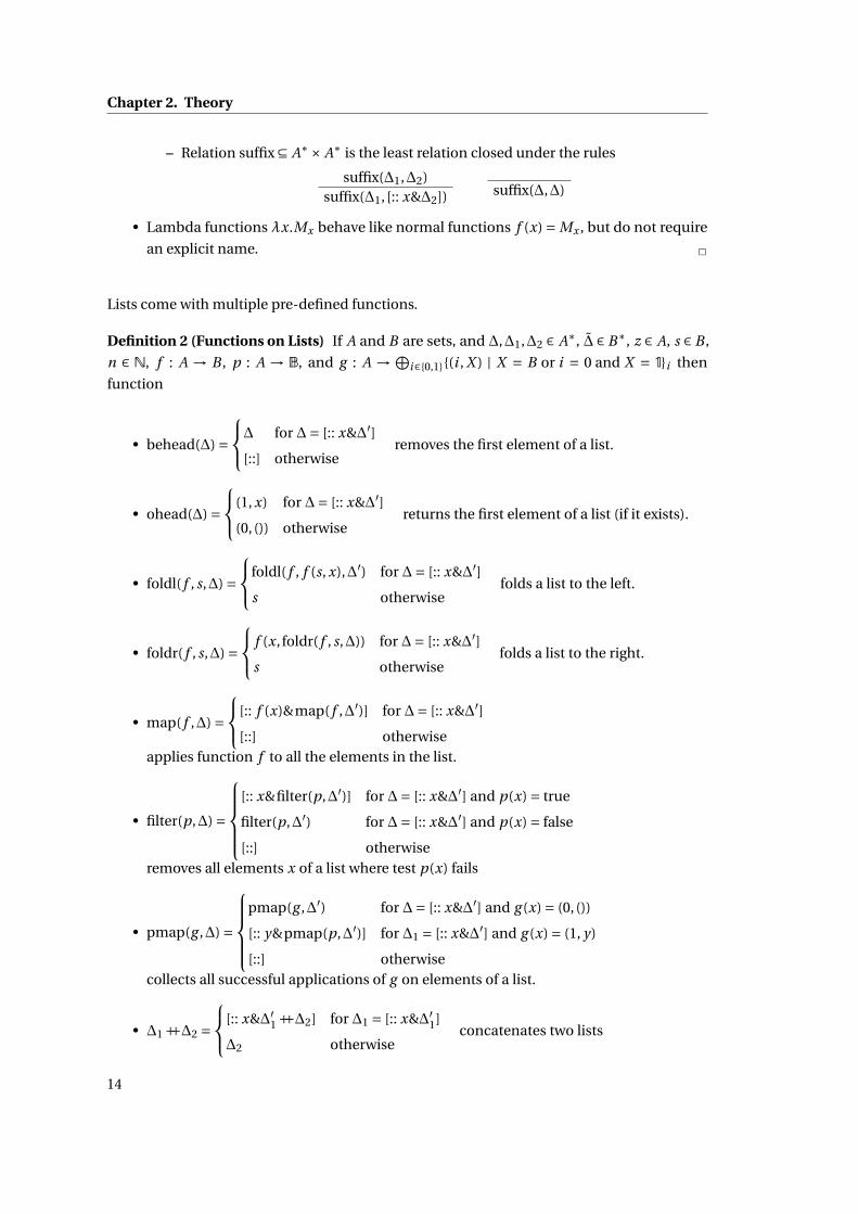
Definition 2 (Functions on Lists) If A and B are sets, and ∆,∆1,∆2 ∈ A∗, ∆ ∈ B∗, z ∈ A, s ∈ B ,
n ∈ N, f : A → B , p : A → B, and g : A → ⨁i∈{0,1}{(i , X ) | X = B or i = 0 and X = 1}i then
function
• behead(∆) =⎧⎨⎩∆ for ∆= [:: x&∆′]
[::] otherwiseremoves the first element of a list.
• ohead(∆) =⎧⎨⎩(1, x) for ∆= [:: x&∆′]
(0, ()) otherwisereturns the first element of a list (if it exists).
• foldl( f , s,∆) =⎧⎨⎩foldl( f , f (s, x),∆′) for ∆= [:: x&∆′]
s otherwisefolds a list to the left.
• foldr( f , s,∆) =⎧⎨⎩ f (x, foldr( f , s,∆)) for ∆= [:: x&∆′]
s otherwisefolds a list to the right.
• map( f ,∆) =⎧⎨⎩[:: f (x)&map( f ,∆′)] for ∆= [:: x&∆′]
[::] otherwiseapplies function f to all the elements in the list.
• filter(p,∆) =
⎧⎪⎪⎪⎨⎪⎪⎪⎩[:: x&filter(p,∆′)] for ∆= [:: x&∆′] and p(x) = true
filter(p,∆′) for ∆= [:: x&∆′] and p(x) = false
[::] otherwiseremoves all elements x of a list where test p(x) fails
• pmap(g ,∆) =
⎧⎪⎪⎪⎨⎪⎪⎪⎩pmap(g ,∆′) for ∆= [:: x&∆′] and g (x) = (0, ())
[:: y&pmap(p,∆′)] for ∆1 = [:: x&∆′] and g (x) = (1, y)
[::] otherwisecollects all successful applications of g on elements of a list.
• ∆1 ++∆2 =⎧⎨⎩[:: x&∆′
1 ++∆2] for ∆1 = [:: x&∆′1]
∆2 otherwiseconcatenates two lists
14

2.1. Formal Verification Setup
• lsize(∆) =⎧⎨⎩1+ lsize(∆′) for ∆= [:: x&∆′]
0 otherwisecomputes the length of a list.
• rcons(∆, z) =⎧⎨⎩[:: x&rcons(∆′, z)] for ∆= [:: x&∆′]
[::z] otherwiseadds an element to the end of a list.
• last(z,∆) =
⎧⎪⎪⎪⎨⎪⎪⎪⎩x for ∆= [::x]
last(z, [:: y&∆′]) for ∆= [:: x&[:: y&∆′]]
z otherwisereturns the last element of a list or its first argument if the list is empty.
• rev(∆) = catrev(∆, [::])
where catrev(∆,∆2) =⎧⎨⎩catrev(∆′, [:: x&∆2]) for ∆= [:: x&∆′]
∆2 otherwisereverses a list.
• zip(∆,∆) =⎧⎨⎩[:: (x, y)&zip(∆′,∆′)] for ∆= [:: x&∆′] and ∆= [:: y&∆′]
[::] otherwisecombines two lists.
• nth(z,∆,n) =
⎧⎪⎪⎪⎨⎪⎪⎪⎩x for n = 0 and ∆= [:: x&∆′]
nth(z,∆′,n′) for n = n′+1 and ∆= [:: x&∆′]
z otherwisereturns the n-th element of a list or the default element z if the list is too short.
• take(n,∆) =⎧⎨⎩[:: x&take(n′,∆′)] for n = n′+1 and ∆= [:: x&∆′]
[::] otherwiseextracts up to n elements from the start of a list.
• subseqs(∆) =⎧⎨⎩map(λ∆′′.[:: x&∆′′],subseqs(∆′))++∆’ for ∆= [:: x&∆′]
[::[::]] otherwise
computes all subsequences ∆′ ⊑∆ of a list ∆.
• nseq(n, z) =⎧⎨⎩[:: z&nseq(n′, z)] for n = n′+1
[::] otherwisereturns a list of n repetitions of z.
• enum(A) = [:: x1&[:: x2&.. . [::xn] . . . ]]
enumerates set A as a list if A is the finite set [:: x1&[:: x2&.. . [::xn] . . . ]]
• undup(∆) =
⎧⎪⎪⎪⎨⎪⎪⎪⎩undup(∆′) for ∆= [:: x&∆′] and x is in ∆′
[:: x&undup(∆′)] for ∆= [:: x&∆′] and not x is in ∆′
[::] otherwiseremoves all duplicates in a list. □
15

Chapter 2. Theory
2.2 Intersection Types with Products and Type Constructors
Prior to any formalization, syntactic conventions for intersection types have to be established.
Definition 3 (Intersection Types with Products and Type Constructors) Intersection types
are formed over the following syntax:
T ∋ A,B ::=ω | c(A) | (A⋆B) | (A → B) | (A∩B)
where c ∈ C is a constructor drawn from a countable set C, which will be chosen per use-case.
Throughout this text, capital Latin letters A,B ,C , . . . are used to denote intersection types,
while small Latin letter denote constructors. Lists of types are denoted by ∆ with some index
or apostrophe for disambiguation. Products ⋆, arrows → and intersections ∩ are to be read
just like their set-theoretic counterparts ×, → and ∩. Parentheses and unnecessary syntax are
reduced using the following conventions:
• Intersections bind stronger than products, which bind stronger than arrows:
A∩B ⋆C → D ×E ∩F = (((A∩B)⋆C ) → (D × (E ∩F )))
• Intersections and arrows associate to the right:
A∩B ∩C → D → E = ((A∩ (B ∩C )) → (D → E))
• Products associate to the left:
A⋆B ⋆C = ((A⋆B)⋆C )
• Constructors with ω-arguments are abbreviated:
c = c(ω)
Equality A = B is strict syntactic equality following the conventions above. □
The syntax presented in Definition 3 is identical to the syntax in [28]. Type constructors are
formally studied in their most generic form with arbitrary arities in [125]. Here, the system
is made more uniform by restricting them to the universal type of anything ω, constructor
symbols applied to one argument, arrows, intersections and a single binary product construc-
tor. This restriction retains the possibility to express interesting types. Notation conventions
highlight that type constants, e.g. int or String, can be represented by having a single ω
argument: int= int(ω) and String= String(ω). Parameterized types such as List(String)
are directly supported. Products can encode multiple parameters, e.g. Graph(N ⋆E) for a
16
2.2. Intersection Types with Products and Type Constructors
graph with nodes of some type N and edges of some type E . Unlike other presentations
[8; 194; 57] there are no type variables. Usually, type variables either model an arbitrary fixed
set of type constants or they are used for schematic polymorphism. The former use-case is
handled by constructor symbols as explained above and no point in the formalization requires
the latter use-case.
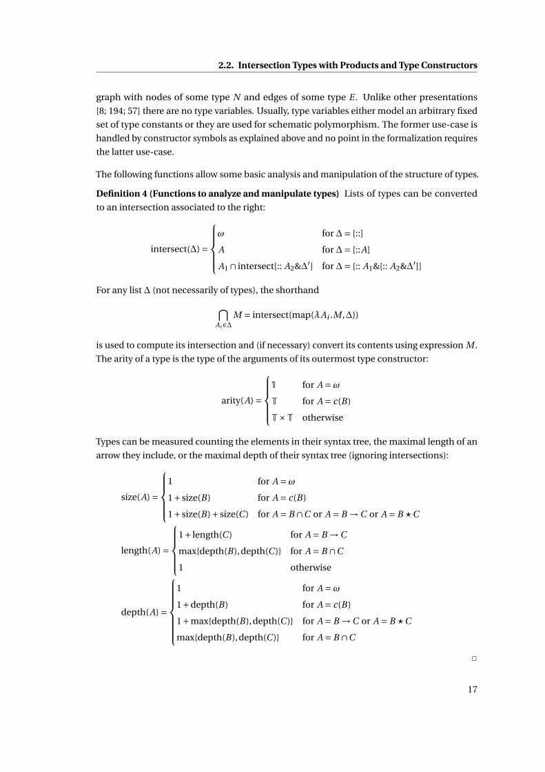
The following functions allow some basic analysis and manipulation of the structure of types.
Definition 4 (Functions to analyze and manipulate types) Lists of types can be converted
to an intersection associated to the right:
intersect(∆) =
⎧⎪⎪⎪⎨⎪⎪⎪⎩ω for ∆= [::]
A for ∆= [::A]
A1 ∩ intersect[:: A2&∆′] for ∆= [:: A1&[:: A2&∆′]]
For any list ∆ (not necessarily of types), the shorthand⋂Ai∈∆
M = intersect(map(λAi .M ,∆))
is used to compute its intersection and (if necessary) convert its contents using expression M .
The arity of a type is the type of the arguments of its outermost type constructor:
arity(A) =
⎧⎪⎪⎪⎨⎪⎪⎪⎩1 for A =ωT for A = c(B)
T×T otherwise
Types can be measured counting the elements in their syntax tree, the maximal length of an
arrow they include, or the maximal depth of their syntax tree (ignoring intersections):
size(A) =
⎧⎪⎪⎪⎨⎪⎪⎪⎩1 for A =ω1+ size(B) for A = c(B)
1+ size(B)+ size(C ) for A = B ∩C or A = B →C or A = B ⋆C
length(A) =
⎧⎪⎪⎪⎨⎪⎪⎪⎩1+ length(C ) for A = B →C
max{depth(B),depth(C )} for A = B ∩C
1 otherwise
depth(A) =
⎧⎪⎪⎪⎪⎪⎪⎨⎪⎪⎪⎪⎪⎪⎩
1 for A =ω1+depth(B) for A = c(B)
1+max{depth(B),depth(C )} for A = B →C or A = B ⋆C
max{depth(B),depth(C )} for A = B ∩C
□
17

Chapter 2. Theory
2.3 Subtyping
The intuition of the intersection type operator ∩ is revealed when types are preordered by
the relation ≤ introduced by Barendregt, Coppo, and Dezani-Ciancaglini [8]. In "A ≤ B" type
A is a subtype of B , meaning that its values can take the shape of values of type B and used
whenever values of type B are expected. This is also referred to as subtype polymorphism.
Relation ≤ is called BCD Subtyping, abbreviating last name initials in honor of its inventors.
Many programming languages are equipped with some similar notion. See [9] for a discussion
of how BCD subtyping can provide a basis for the formalization of other subtype relations.
Also Section 2.6 will come back to this point.
Definition 5 (BCD Subtyping) The subtype relation A ≤ B is the least relation closed under
the rules:
c ≤C d A ≤ B(CAX)
c(A) ≤ d(B)(CDIST)
c(A)∩ c(B) ≤ c(A∩B)
(ω)A ≤ω (→ω)ω≤ω→ω
B1 ≤ A1 A2 ≤ B2 (SUB)A1 → A2 ≤ B1 → B2
(DIST )(A → B1)∩ (A → B2) ≤ A → B1 ∩B2
A1 ≤ B1 A2 ≤ B2 (PRODSUB)A1⋆ A2 ≤ B1⋆B2
(PRODDIST )(A1⋆ A2)∩ (B1⋆B2) ≤ A1 ∩B1⋆ A2 ∩B2
A ≤ B1 A ≤ B2 (GLB)A ≤ B1 ∩B2
(LUB1)B1 ∩B2 ≤ B1
(LUB2)B1 ∩B2 ≤ B2
A ≤ B B ≤C ( TRANS)A ≤C
(REFL)A ≤ A
where ≤C is an arbitrary fixed preorder chosen together with the constructor symbols C. □
Rules (CAX), (CDIST), (PRODSUB), and (PRODDIST) are extensions to the original relation [8]
and account for the extended set of intersection types used in this text. The extensions are
again a restriction of those studied in [125]. Rule (ω) positions type ω as the universal type
of any value. This is analogous to the type Object in Java or C#. Rule (→ω) accounts for the
lack of information on functions where the only known property is that they compute ω, i.e.
anything. Combined with rule (ω) this information is equally (un-)specific as the information
18

2.3. Subtyping
that such a function could be anything. Rule (SUB) expresses the subtype polymorphism
property for functions. A function of type A1 → A2 is usable in place of a function of type
B1 → B2 if it operates on less specific inputs (B1 ≤ A1, contravariance) and produces more
specific outputs (A2 ≤ B2, covariance). Note how rule (PRODSUB) is the same for products
with the crucial difference that components A1 and B1 are also covariant (A1 ≤ B1) in its
first premise. Similarly, unary constructors are ordered by (CAX). Here, the first premise is
replaced by a customizable relation ≤C⊆ C×C that can be chosen with the set of constructor
symbols C. This extension mechanism provides the basis for embedding signature subsorting
in Section 2.6. Rules (GLB), (LUB1), and (LUB2) turn the intersection operator ∩ into the
meet of a semi-lattice [86]. If values of type A can be used for B1 and B2, they can be used
whenever the intersection B1 ∩B2 is expected. Vice versa, values of the intersection of types
B1 and B2 can be used as values of both of these types. These rules are compatible with
interpreting types as sets of values with ≤ as subset inclusion ⊆ and ∩ as the intersection of sets.
Rules (DIST), (CDIST), and (PRODDIST) allow distribution of intersections over covariantly
related type components. Distribution over the contravariant left component of arrows
(A1 → B1)∩ (A2 → B2) ≤ A1 ∩ A2 → B1 ∩B2 is derivable from the other rules and does not need
to be explicitly included. Finally (TRANS) and (REFL) close ≤ under transitivity and reflexivity,
turning it into a preorder. Equivalent formulations of the rules above are discussed in [194].
The decision problem for the BCD Subtype relation is the following: given two types A and B ,
are they related by A ≤ B? At first glance, most rules of the subtype relation seem to indicate
that a decision procedure can simply try to construct a proof tree by reading the rules from
conclusion to premise. However, this approach breaks down because of type B in rule (TRANS),
which is not present in the conclusion and would thus have to be guessed. Rules with variables
in their premises that do not occur in their conclusion are called called cut-rules and B is
called a cut-type. Reformulating a proof system without cut rules is called cut-elimination and
the textbook example of cut-elimination is Gentzen’s Hauptsatz [176]. Laurent [125] proves
that cut elimination is possible for the rules of ≤. Solutions to the BCD Subtype decision
problem can be traced along a line of work started over 30 years ago with a decidability
proof by Pierce [156]. It was subsequently improved to decision procedures with exponential
worst-case runtime [45; 46; 118]. Later, algorithms with polynomial O (n4) [165] and O (n5)
[180] runtimes have been obtained. The first procedure with quadratic runtime O (n2) was
developed in [67]. Algorithms with mechanized proofs but without runtime guarantees have
followed [24; 125; 30], where issues with the original proof have been discovered in [30]. The
decision procedure used in this text is the first with formally verified quadratic bounds on the
number of recursive steps involved to find a solution. At the time of writing a detailed account
of its development is peer-reviewed and accepted for publication [28] with authorship of the
presented parts of that publication coinciding with the declared authorship of this text.
Besides the aforementioned cut in rule (TRANS), the most difficult part in designing and
verifying a decision procedure for ≤ is created by the first premise in rule (SUB). It toggles the
positions of types to B1 ≤ A1 instead of A1 ≤ B1. This effectively prevents structural recursion
on types from working and more advanced techniques have to be employed for ensuring
19

Chapter 2. Theory
termination. Larchey-Wendling and Monin [123] suggest a way to obtain a termination
certificate Dom that allows recursion decreasing on its structure for such situations. The trick
is to turn a proof about a recursively defined function f into a proof about an inductively
defined relation R. The relation is then proven to be functional (xR y1 and xR y2 implies
y1 = y2). Termination certificate Dom x is defined to be a proof tree for the statement that
there exists y such that xR y (x is in the domain of the relation). If Dom is total (for all x there
exists a proof Dom x) function f can then be defined by structural recursion on the proof tree
Dom x for any input x. Bounding the size of Dom puts a bound on the number of recursive
calls in f , yielding information about worst case performance. Inductively defining R is also
a good way to understand the algorithm: it effectively specifies its operational semantics by
means of rules for each possible input. This is useful for debugging purposes, because the
algorithm can be "halted" at each rule invocation. Furthermore, the relation provides an
alternative cut-free representation for ≤.
Some auxiliary functions are required for the main decision procedure.
Definition 6 (Auxiliary functions to decide BCD Subtyping) Testing for ω≤ A is purely syn-
tactic:
isOmega(A) =
⎧⎪⎪⎪⎪⎪⎪⎨⎪⎪⎪⎪⎪⎪⎩
true for A =ωisOmega(A2) for A = A1 → A2
isOmega(A1) and isOmega(A2) for A = A1 ∩ A2
false otherwise
Function castB : T→ arity(B) collects type components to be recursively compared when
checking A ≤ B . Its helper function cast′B avoids inefficient functional list concatenations
using an accumulator parameter ∆.
castB (A) =
⎧⎪⎪⎪⎨⎪⎪⎪⎩[::ω] for B =ω[::(ω,ω)] for B = B1 → B2 and isOmega(B2)
cast′B (A, [::]) otherwise
cast′B (A,∆) =
⎧⎪⎪⎪⎪⎪⎪⎪⎪⎪⎨⎪⎪⎪⎪⎪⎪⎪⎪⎪⎩
[:: A′&∆] for A = c(A′) and B = d(B ′) and c ≤C d
[:: (A1, A2)&∆] for A = A1 → A2 and B = B1 → B2
[:: (A1, A2)&∆] for A = A1⋆ A2 and B = B1⋆B2
cast′B (A1,cast′B (A2,∆)) for A = A1 ∩ A2
∆ otherwise
□
The relational specification of subtyping can be thought of as a machine performing steps to
transform inputs to outputs.
20

2.3. Subtyping
Definition 7 (BCD Subtype Machine) The BCD Subtype relation is decided by a machine
transforming inputs
ISub ∋ i ::= [ subty A of B ] | [ tgt_for_srcs_gte A in ∆]
to outputs
OSub ∋ o ::= [ Return b] | [ check_tgt ∆′]
where b is a Boolean, A,B ∈T, ∆ is a list of pairs of types, and ∆′ is a list of types.
Its operational semantics is specified by the least relation ↝⊂ ISub ×OSub closed under the
following rules:
(STEPω)[ subty A of ω]↝ [ Return true]
[ subty⋂
Ai∈castc(B)(A) Ai of B ]↝ [ Return b](STEPCTOR)
[ subty A of c(B)]↝ [ Return castc(B)(A) = [::] and b]
[ subty⋂
Ai∈castB1⋆B2 (A) Ai .1 of B1]↝ [ Return b1]
[ subty⋂
Ai∈castB1⋆B2 (A) Ai .2 of B2]↝ [ Return b2](STEP⋆)
[ subty A of B1 ×B2]↝ [ Return castB1⋆B2 (A) = [::] and b1 and b2]
[ tgt_for_srcs_gte B1 in castB1→B2 (A)]↝ [ check_tgt ∆]
[ subty⋂
Ai∈∆Ai of B2]↝ [ Return b]
(STEP→)[ subty A of B1 → B2]↝ [ Return isOmega(B2) or b]
[ subty B of A.1]↝ [ Return b]
[ tgt_for_srcs_gte B in ∆]↝ [ check_tgt ∆′](STEPCHOOSETGT)
[ tgt_for_srcs_gte B in [:: A&∆]]↝
[ check_tgt if b then [:: A.2&∆′] else ∆′]
(STEPDONETGT)[ tgt_for_srcs_gte B in [::]]↝ [ check_tgt [::]]
[ subty A of B1]↝ [ Return b1]
[ subty A of B2]↝ [ Return b2](STEP∩)
[ subty A of B1 ∩B2]↝ [ Return b1 and b2]
□
21

Chapter 2. Theory
Behavior of the subtype machine can be explained considering each rule individually: Rule
(STEPω) is just rule (ω) from the BCD relation. Constructors are analyzed recursively by
(STEPCTOR). Auxiliary function castc(B) collects all arguments to recursively compare. For
example, if d ≤C c, f ≤C c, and not e ≤C c the result of casting is castc(B)(d(A1) ∩ (A2 →A3)∩ e(A4)∩ f (A5)) = [:: A1&[::A5]]. If the list returned by cast is empty, either type shapes
did not match or there was no compatible constructor symbol. It is crucial to check this,
because the premise [ subty⋂
Ai∈castc(ω)(A) Ai of ω] ↝ [ Return b] is fulfilled for any A,
even if it is structurally fully incompatible with c(ω), e.g. A = (A1⋆ A2)∩ (A3 → A4). Formal
verification in Coq spotted forgetting this check at an early stage of development. Rule
(STEP⋆) for the product constructor is analogous to (STEPCTOR). Arrows are more difficult
to process because of the aforementioned switch in variance of their first argument. Three
rules are required. The entry point, (STEP→), ensures subtyping of the second argument and
identifies arrows collapsing to ω using isOmega. The second argument cannot be directly
compared. If multiple arrows are present in A, their distribution by (DIST) can be required for
subtyping. However, just collecting all targets in A does not work: if A ≤ A1, A ≤ A2, and not
A ≤ A3 distribution in (A1 → B1)∩ (A2 → B2)∩ (A3 → B3) results in A1∩ A2∩ A3 → B1∩B2∩B3
which is not a subtype of A → B1 ∩B2, even though just distributing the first two arrows
results in (A1 → B1)∩ (A2 → B2)∩ (A3 → B3) ≤ A1 ∩ A2 → B1 ∩B2 ≤ A → B1 ∩B2. Instruction
[ tgt_for_srcs_gte B1 in castB1→B2 (A)] in the first premise of (STEP→) is responsible for
selecting the correct arrows in A. Rules (STEPCHOOSETGT) and (STEPDONETGT) implement this
computation. If the input list created by castB1→B2 (A) is fully processed or empty no additional
arrow target is to be selected (STEPDONETGT). If there is a remaining arrow, its first argument is
compared to B1 and the second argument is added to the list of targets to compare if this check
is successful. In the above example, this results in B1 and B2 being added to ∆′ while B3 is
dropped. The final rule (STEP∩) is an implementation of (GLB): components of intersections
are just recursively compared. Unlike ≤, relation ↝ does not include cut rules and the choice
of rule to apply is fully determined by the input instruction. The following proofs will establish
that ↝ can be implemented by a recursively defined function and that it is correct (sound and
complete) with respect to relation ≤.
Lemma 1 (Functionality of the BCD Subtype Machine) For all instructions i ∈ ISub and out-
puts o1,o2 ∈OSub, if i ↝ o1 and i ↝ o2 then o1 = o2.
PROOF Induction on the proof of i ↝ o1 followed by case analysis on i ↝ o2 ■
The termination certificate Dom can be defined next.
Definition 8 (Termination certificate for the BCD Subtype Machine) For any input i ∈ ISub,
termination certificate Dom i is a finite proof tree constructed from the following rules:
Dom[ subty A of ω]
1 Dom[ subty⋂
Ai∈castc(B)(A) Ai of B ]
Dom[ subty A of c(B)]
22

2.3. Subtyping
1 Dom[ tgt_for_srcs_gte B1 in castB1→B2 A]
2 for all ∆, if [ tgt_for_srcs_gte B1 in castB1→B2 A]↝ [ check_tgt ∆]
then Dom[ subty⋂
Ai∈∆Ai of B2]
Dom[ subty A of B1 → B2]
1 Dom[ subty B of A.1] 2 Dom[ tgt_for_srcs_gte B in ∆]
Dom[ tgt_for_srcs_gte B in [:: A&∆]]
Dom[ tgt_for_srcs_gte B in [::]]
1 Dom[ subty⋂
Ai∈castB1⋆B2 (A) Ai .1 of B1]
2 Dom[ subty⋂
Ai∈castB1⋆B2 (A) Ai .2 of B2]
Dom[ subty A of B1⋆B2]
1 Dom[ subty A of B1]
2 Dom[ subty A of B2]
Dom[ subty A of B1 ∩B2]
Childproofs of a tree p ∈ Dom i are selected using p.1 and p.2 where the boxed number in
front of each premise specifies which projection is chosen. □
The rules of Dom closely follow those of ↝. Each recursive use of ↝ is modeled by a child
proof in Dom, while other information - especially the result value - is erased. This leads to
Dom being just weak enough to poof totality.
Lemma 2 Totality of the Termination Certificate Dom For all instructions i ∈ ISub there exists a
proof tree Dom i .
PROOF First if A is ω, Dom[ subty ω of B ] is obtained by induction on the structure of B .
For the other cases, induction on the maximal depth of A and B is followed by induction on
the structure of B . Function castB (A) either returns components with a smaller depth than
A, or [::ω] or [::(ω,ω)]. The ω-cases are dispatched by the earlier proof. Otherwise the list
returned by castB (A) contains only types with depth less than A. For (STEPCTOR), (STEP⋆), and
(STEP∩) the induction hypotheses solve the goal. For rule (STEP→) target collection in the first
premise is shown to compute a list of targets with depth less than A by induction on the length
of castB1→B2 (A) using the outer induction hypothesis for checking if B1 is a subtype of any
of the sources. This is possible in spite of the toggled position of B1, because the maximal
depth of types A and B ignores the order of A and B . Any target list returned by invocations
of (STEPCHOOSETGT) and (STEPDONETGT) only contains targets produced by cast castB1→B2 (A)
and their intersection has a depth smaller than B2, because depth does not increase when
performing intersection operations. This is sufficient to complete the proof for the second
premise of (STEP→) using the induction hypotheses. ■
23

Chapter 2. Theory
Functionality and totality are enough to translate the operational semantics ↝ into denota-
tional semantics, a recursive procedure to decide subtyping.
Definition 9 (Procedure deciding the BCD Subtype Relation)
subtypes(i ∈ ISub) : Dom i → {o ∈OSub | i ↝ o}
subtypes(i )(p) =⎧⎪⎪⎪⎪⎪⎪⎪⎪⎪⎪⎪⎪⎪⎪⎪⎪⎪⎪⎪⎪⎪⎪⎪⎪⎪⎪⎪⎪⎪⎪⎪⎪⎪⎪⎪⎪⎪⎪⎪⎪⎪⎪⎪⎪⎪⎪⎪⎪⎪⎪⎪⎪⎪⎪⎪⎪⎪⎪⎪⎪⎪⎪⎪⎪⎪⎪⎪⎪⎪⎨⎪⎪⎪⎪⎪⎪⎪⎪⎪⎪⎪⎪⎪⎪⎪⎪⎪⎪⎪⎪⎪⎪⎪⎪⎪⎪⎪⎪⎪⎪⎪⎪⎪⎪⎪⎪⎪⎪⎪⎪⎪⎪⎪⎪⎪⎪⎪⎪⎪⎪⎪⎪⎪⎪⎪⎪⎪⎪⎪⎪⎪⎪⎪⎪⎪⎪⎪⎪⎪⎩
[ Return true] if i = [ subty A of ω]
[ Return castc(B)(A) = [::] and b]
if i = [ subty A of c(B)] and
for A′ :=⋂castc(B)(A) Ai
subtypes([ subty A′ of B ])(p.1) = [ Return b]
[ Return isOmega(B2) or b]
if i = [ subty A of B1 → B2] and
for A1 := castB1→B2 (A)
subtypes([ tgt_for_srcs_gte B1 in A1])(p.1) =[ check_tgt ∆] and
for A2 :=⋂Ai∈∆ Ai
subtypes([ subty A2 of B2])(p.2) = [ Return b]
[ Return castB1⋆B2 (A) = [::] and b1 and b2]
if i = [ subty A of B1⋆B2] and
for A1 :=⋂Ai∈castB1⋆B2 (A) Ai .1
subtypes([ subty A1 of B1])(p.1) = [ Return b1] and
for A2 :=⋂Ai∈castB1⋆B2 (A) Ai .2
subtypes([ subty A2 of B2])(p.2) = [ Return b2]
[ Return b1 and b2]
if i = [ subty A of B1 ∩B2] and
subtypes([ subty A of B1])(p.1) = [ Return b1] and
subtypes([ subty A of B2])(p.2) = [ Return b2]
[ check_tgt if b then [:: A.2&∆′] else ∆′]
if i = [ tgt_for_srcs_gte B in [:: A&∆]] and
subtypes([ subty B of A.1])(p.1) = [ Return b] and
subtypes([ tgt_for_srcs_gte B in ∆])(p.2) =[ check_tgt ∆′]
[ check_tgt [::]] if i = [ tgt_for_srcs_gte B in [::]]
□
Each case in function subtypes implements a rule of ↝. It thus respects its restricted range
{o ∈ OSub | i ↝ o}. Recursive calls always use a child trees of p ∈ Dom i and thus terminate
24
2.3. Subtyping
because p is finite. Lemma 2 ensures existence of p for any input instruction i . Lemma 1
proves that subtypes does not lose any solutions. In Coq the termination certificate is part of
the universe of propositions, which is erased when extracting the specification to an executable
functional target language such as Haskell or OCaml: The constructive proof of Lemma 2 is
enough to ensure Dom proof trees exist and can be constructed without actually ever wasting
resources for constructing them. Most executable programming languages accept recursive
definitions without totality proofs and eliminate this overhead.
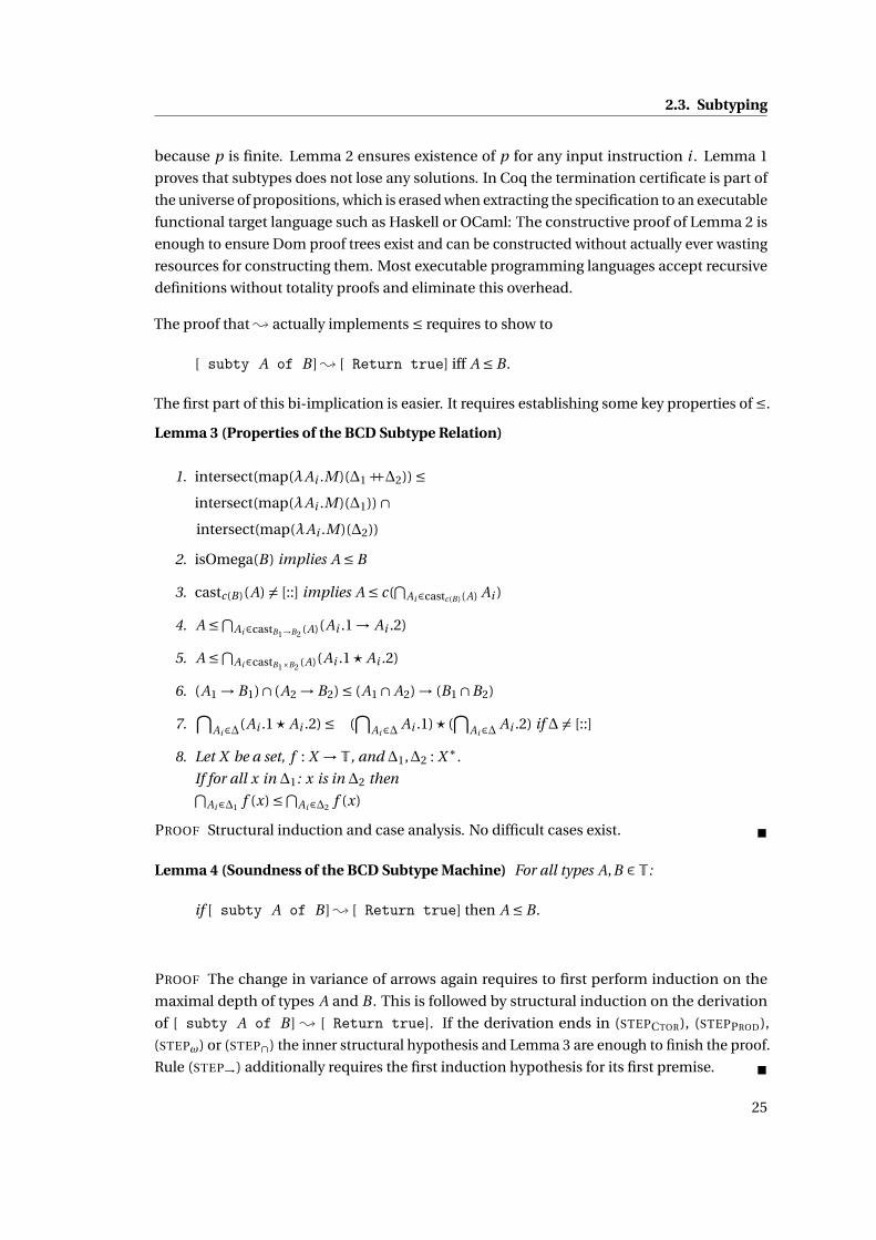
The proof that ↝ actually implements ≤ requires to show to
[ subty A of B ]↝ [ Return true] iff A ≤ B.
The first part of this bi-implication is easier. It requires establishing some key properties of ≤.
Lemma 3 (Properties of the BCD Subtype Relation)
1. intersect(map(λAi .M)(∆1 ++∆2)) ≤intersect(map(λAi .M)(∆1)) ∩intersect(map(λAi .M)(∆2))
2. isOmega(B) implies A ≤ B
3. castc(B)(A) = [::] implies A ≤ c(⋂
Ai∈castc(B)(A) Ai )
4. A ≤⋂Ai∈castB1→B2 (A)(Ai .1 → Ai .2)
5. A ≤⋂Ai∈castB1×B2 (A)(Ai .1⋆ Ai .2)
6. (A1 → B1)∩ (A2 → B2) ≤ (A1 ∩ A2) → (B1 ∩B2)
7.⋂
Ai∈∆(Ai .1⋆ Ai .2) ≤ (⋂
Ai∈∆ Ai .1)⋆ (⋂
Ai∈∆ Ai .2) if ∆ = [::]
8. Let X be a set, f : X →T, and ∆1,∆2 : X ∗.
If for all x in ∆1: x is in ∆2 then⋂Ai∈∆1
f (x) ≤⋂Ai∈∆2
f (x)
PROOF Structural induction and case analysis. No difficult cases exist. ■
Lemma 4 (Soundness of the BCD Subtype Machine) For all types A,B ∈T:
if [ subty A of B ]↝ [ Return true] then A ≤ B.
PROOF The change in variance of arrows again requires to first perform induction on the
maximal depth of types A and B . This is followed by structural induction on the derivation
of [ subty A of B ] ↝ [ Return true]. If the derivation ends in (STEPCTOR), (STEPPROD),
(STEPω) or (STEP∩) the inner structural hypothesis and Lemma 3 are enough to finish the proof.
Rule (STEP→) additionally requires the first induction hypothesis for its first premise. ■
25

Chapter 2. Theory
The proof of completeness requires to show that ↝ supports transitivity of subtyping as well
as several other properties established by the following lemma.
Lemma 5 (Properties of the BCD Subtype Machine)
1. isOmega(B) implies [ subty A of B ]↝ [ Return true]
2. [ tgt_for_srcs_gte B1 in ∆]↝ [ check_tgt ∆′] implies
∆′ ⊑ map(λAi .Ai .2)(∆)
3. [ tgt_for_srcs_gte B1 in castB1→B2 A]↝ [ check_tgt ∆] and
isOmega(A) implies isOmega(Ai ) for all Ai in ∆
4. [ subty A of B ]↝ [ Return true] and isOmega(A) implies isOmega(B)
5. ∆2 ⊑∆1 and [ tgt_for_srcs_gte B1 in ∆1]↝ [ check_tgt ∆′1] and
[ tgt_for_srcs_gte B1 in ∆2]↝ [ check_tgt ∆′2] implies ∆′
2 ⊑∆′1
6. ∆⊑∆′ and [ subty⋂
Ai∈∆ Ai of A]↝ [ Return true] implies
[ subty⋂
Bi∈∆′ Bi of A]↝ [ Return true]
7. [ subty A of⋂
Ai∈∆1Ai ]↝ [ Return b1] and
[ subty A of⋂
Ai∈∆2Ai ]↝ [ Return b2] implies
[ subty A of⋂
Ai∈∆3Ai ]↝ [ Return b1 ∧b2] for ∆3 =∆1 ++∆2
8. [ subty A of B ]↝ [ Return true] implies
[ subty⋂
Ai∈castc(C ) A Ai of⋂
Bi∈castc(C )B Bi ]↝ [ Return true]
9. [ tgt_for_srcs_gte B in [::(ω, A)]]↝ [ check_tgt ∆] implies ∆= [::A]
10. [ subty A of A]↝ [ Return true]
11. [ tgt_for_srcs_gte A in ∆1]↝ [ check_tgt ∆′1] and
[ tgt_for_srcs_gte A in ∆2]↝ [ check_tgt ∆′2] implies
[ tgt_for_srcs_gte A in ∆3]↝ [ check_tgt ∆′3] for
∆3 =∆1 ++∆2 and ∆′3 =∆′
1 ++∆′2
12. [ tgt_for_srcs_gte A in ∆1 ++∆2]↝ [ check_tgt ∆′] implies
there exist ∆′1,∆′
2, s.t.
[ tgt_for_srcs_gte A in ∆1]↝ [ check_tgt ∆′1] and
[ tgt_for_srcs_gte A in ∆2]↝ [ check_tgt ∆′2] and
∆′ =∆′1 ++∆′
2
13. [ subty A of B1 ∩B2]↝ [ Return true] implies
[ subty A of B1]↝ [ Return true] and [ subty A of B2]↝ [ Return true]
14. C = c(C ′) or C =C1⋆C2 and castC B = [::] and
[ subty A of B ]↝ [ Return true] implies
castC A = [::]
26

2.3. Subtyping
15. [ subty A of B ]↝ [ Return true] and
[ subty B of C ]↝ [ Return true] implies
[ subty A of C ]↝ [ Return true]
16. [ subty c(A1)∩ c(A2) of c(A1 ∩ A2)]↝ [ Return true]
17. [ subty A∩ A of A]↝ [ Return true]
PROOF The statements are proven in the order they are presented. Most just require induction
and/or case analysis. The weakening property in case 6 is inspired by [125]. It is needed for the
reflexivity proof for A = A1∩A2. Transitivity in case 14 again needs nested structural induction
with an outer induction on the maximum of the depth of the types involved. ■
Lemma 6 (Completeness of the BCD Subtype Machine) For all types A,B ∈T:
if A ≤ B then [ subty A of B ]↝ [ Return true].
PROOF Induction on the derivation of A ≤ B using Lemma 5. Lemma 5.14 takes care of the
problematic transitivity rule (TRANS). ■
Correctness of the decision procedure in Definition 8 can now be proven.
Theorem 1 (Subtype decision procedure correctness) For all A,B ∈T there exists a termina-
tion certificate p ∈ Dom[ subty A of B ].
For all termination certificates p ∈ Dom[ subty A of B ] there exists a Boolean b such that
subtypes([ subty A of B ])(p) = [ Return b] with b = true if and only if A ≤ B.
PROOF The first part is Lemma 2. In the second part subtypes([ subty A of B ])(p) =[ Return b] and b = tr ue can be replaced by either [ subty A of B ] ↝ [ Return true]
or [ subty A of B ]↝ [ Return false] because of the definition of subtypes and function-
ality of ↝. The result then immediately follows from Lemma 4 and Lemma 6. ■
Further analysis of the termination certificate provides some insight on a bound of the number
of possible recursive calls.
Lemma 7 (Size of the Termination Certificate) For i ∈ ISub, p ∈ Domi define
measurei (p) =
⎧⎪⎪⎪⎪⎪⎪⎨⎪⎪⎪⎪⎪⎪⎩
1 for i = [ subty A of ω] or
[ tgt_for_srcs_gte B in [::]]
1+measure(p.1) for i = [ subty A of c(B)]
1+measure(p.1)+measure(p.2) otherwise
27

Chapter 2. Theory
and obtain
measurei (p) ≤
⎧⎪⎪⎪⎨⎪⎪⎪⎩2 · size(A) · size(B) for i = [ subty A of B ]
1+ size(B) ·∑kj=1(1+2 · size(A j .1))
for i = [ tgt_for_srcs_gte B in [:: A1&[:: A2&.. . [::Ak ] . . . ]]]
PROOF The key insight is that types returned by castB (A) always have sizes smaller or equal
than the size of A. The result then follows by induction on p with a special case for i =[ subty A of B1 → B2] where B2 =ω and costi (p) ≤ 3. ■
Kurata and Takahashi [118] identified an algorithmically important property of the restricted
set of types considered in precursors to the full BCD system [43]. This property has been
the basis for the algorithms presented in [165] and has been algebraically classified [24] as
primality of the ideal induced by ≤.
Definition 10 (Primality) The ideal of A ∈T is the non-empty set {B ∈T|B ≤ A} and A is its
principal element. An ideal with principal element C is prime if for all A∩B in the ideal, A ≤C
or B ≤C . Type C is prime if it is the principal element of a prime ideal. □
Prime ideals are desirable because they avoid distribution. For example if C prime, then in
(A1 → B1)∩ (A2 → B2) ≤ C the distribution (A1 ∩ A2 → B1 ∩B2) ≤ C never has to be taken
into account, because one of the types (A1 → B1) and (A2 → B2) is less than C . One of the
particularly beautiful facts about intersection types is that primality is a purely syntactic
criterion and the precursor system [43] correctly captured that notion. Here, the syntactic
criterion is extended to account for constructor symbols and products.
Lemma 8 (Syntactic criterion for Primality) The set
T⊃Tωπ ∋π ::=ω | c(π) | (ω⋆π) | (π⋆ω) | A →π
is identical to the set of prime types.
PROOF By Lemma 4 and Lemma 6 it is sufficient to show
[ subty A∩B of π]↝ [ Return true] implies
[ subty A of π]↝ [ Return true] or
[ subty B of π]↝ [ Return true]
Induction on C uniquely identifies the last rule used to derive [ subty A ∩ B of π] ↝
[ Return true] in each case and the result then easily follows. ■
Let Tπ = {π ∈ Tωπ | not isOmega(π)} denote the set of prime types that do not collapse to ω
under subtyping. In [43] this set is called the set of tail-proper types. In [57] and [67] these
types are called paths and it is proven that every type can be organized into a subtype equal
set of paths.
28

2.3. Subtyping
Definition 11 (Prime factorization of Types) The following function computes a minimal
sequence of prime factors of type A ∈T:
primeFactors(A) = primeFactors′(A, id, [::])
primeFactors′(A,contextualize,∆) =⎧⎪⎪⎪⎪⎪⎪⎪⎪⎪⎪⎪⎪⎪⎪⎪⎪⎪⎪⎪⎪⎪⎨⎪⎪⎪⎪⎪⎪⎪⎪⎪⎪⎪⎪⎪⎪⎪⎪⎪⎪⎪⎪⎪⎩
∆ for A =ω and
isOmega(contextualize(A))
addAndFilter(∆,contextualize(A)) for A =ω and not
isOmega(contextualize(A))
primeFactors′(A′,λB.contextualize(c(B)),∆) for A = c(A′)
primeFactors′(A2,λB.contextualize(A1 → B),∆) for A = A1 → A2
primeFactors′(A2,λB.contextualize(ω⋆B),
primeFactors′(A1,λB.contextualize(B ⋆ω),∆))
for A = A1⋆ A2
primeFactors′(A2,contextualize,
primeFactors′(A1,contextualize,∆))
for A = A1 ∩ A2
addAndFilter(∆, A) =⎧⎪⎪⎪⎪⎪⎪⎨⎪⎪⎪⎪⎪⎪⎩
[::A] for ∆= [::]
[:: B&∆′] for ∆= [:: B&∆′] and B ≤ A
addAndFilter(∆′, A) for ∆= [:: B&∆′] and not B ≤ A and A ≤ B
[:: B&addAndFilter(∆′, A)] otherwise
□
Function primeFactors is implemented using primeFactors′, which keeps track of the accu-
mulated list of prime factors ∆ and the context of the currently analyzed type with regard to
the initial type. This context is represented as a function mapping the current type into the
structure of the parent type. The context representation is inspired by Zippers, a functional
programming technique [104; 101]. Recursion in primeFactors′ finishes when ω is reached. If
ω is less or equal than the computed prime factor at this point, it is redundant, just like 1 is
redundant as a prime factor in a natural number. Otherwise it is inserted into the list of prime
factors using addAndFilter. Function addAndFilter appends a prime factor A to a list of prime
factors∆ if that list contains no subtype related element. Otherwise, if there is such an element,
and it is smaller than A, ∆ remains constant. If the existing element is greater than A, it will be
replaced. The result of addAndFilter is a minimal list of prime factors without duplication of
subtype equal types. In any case which is not ω, function primeFactors′ recursively proceeds,
adapting the context with the operation to map the next considered argument back into place.
Products have to be split recontextualizing their left and right prime components separately,
setting the other component to ω (c.f. the restricted shape of products in Tπ). The following
lemma is necessary to establish correctness and minimality of primeFactors.
29

Chapter 2. Theory
Lemma 9 (Prime factorization verification properties)
Let ∆,∆1,∆2,∆3,∆′ be universally quantified lists of types and A,B ,C ,D ∈T, then:
1. There exists some B in addAndFilter(∆, A), s.t. B ≤ A
2. There exists some A′ in addAndFilter(∆, A), s.t. A′ ≤C iff A ≤C or there exists B ′ in ∆ s.t.
B ′ ≤C .
3. If ∆ ⊑ ∆′ and there exists A′ in addAndFilter(∆, A) s.t. A′ ≤ B then there exists A′′ in
addAndFilter(∆′, A) s.t. A′′ ≤ B
4. If B is in addAndFilter(∆, A) then B = A or B is in ∆
5. If A is in ∆ and A ≤ B then⋂
Ai∈∆ Ai ≤ B
6.⋂
Ai∈addAndFilter(∆,A) Ai ≤⋂Ai∈∆ Ai
7. Let P :T→B then for all A in ∆: P(A) implies for all B in addAndFilter(∆): P(B)
8. If for all A in ∆: A ∈Tπ and for all B ∈Tπ: contextualize(B) ∈Tπ then
for all D in primeFactors′(C ,contextualize,∆): D ∈Tπ9.
⋂Ai∈primeFactors′(A,contextualize,∆) Ai ≤⋂
Ai∈∆ Ai
10. If for all B ,C ∈T: B ≤C implies
contextualize(B) ≤ contextualize(C ) and
contextualize(B)∩contextualize(C ) ≤ contextualize(B ∩C ) then⋂Ai∈primeFactors′(A,contextualize,∆) Ai ≤ A
11. If B is in addAndFilter(∆, A) then there exists C in [:: A&∆] s.t. C ≤ B
12. If for all A in ∆2 there exists B in ∆1 s.t. B ≤ A then⋂
Ai∈∆1Ai ≤⋂
Ai∈∆2Ai
13.⋂
Ai∈[::A&∆] Ai ≤⋂Ai∈addAndFilter(∆,A) Ai
14. If for all B ,C ∈T: B ≤C implies contextualize(B) ≤ contextualize(C ) then⋂Ai∈[::A&∆] Ai ≤⋂
Ai∈primeFactors′(A,contextualize,∆) Ai
Define lists free of subtype equal duplicates
nosubdup(∆) =
⎧⎪⎪⎨⎪⎪⎩true for ∆= [::]
nosubdup(∆′) and
for all B in ∆ : not A ≤ B and not B ≤ A
for ∆= [:: A&∆′]
15. nosubdup(∆) implies nosubdup(addAndFilter(∆, A))
16. nosubdup(∆) implies nosubdup(primeFactors′(A,contextualize,∆))
30

2.3. Subtyping
17. If for all A in∆: notω≤ A then for all B in primeFactors′(A,contextualize,∆): notω≤ A
Define deduplication modulo subtyping
desubdup(∆) =
⎧⎪⎪⎪⎨⎪⎪⎪⎩[::] for ∆= [::]
addAndFilter(desubdup(∆′), A) for ∆= [:: A&∆′] and not isOmega(A)
desubdup(∆′) for ∆= [:: A&∆′] and isOmega(A)
18. nosubdup(desubdup(∆))
19. Let P :T→B then for all A in ∆: P(A) implies for all B in desubdup(∆): P(B)
20.⋂
Ai∈desubdup(∆) Ai ≤⋂Ai∈∆ Ai
21.⋂
Ai∈∆ Ai ≤⋂Ai∈desubdup(∆) Ai
22. lsize(addAndFilter(∆)) ≤ lsize(∆)
23. lsize(desubdup(∆)) ≤ lsize(∆)
24. If A in desubdup(∆) then not isOmega(A)
25. If⋂
Ai∈∆1Ai ≤⋂
Ai∈∆2Ai and
for all A in ∆2: A ∈Tπ and not isOmega(A) then
for all A in ∆2: exists B in ∆1, s.t. B ≤ A
26. If⋂
Ai∈∆1Ai ≤⋂
Ai∈∆2Ai and
for all A in ∆2: A ∈Tπ and not isOmega(A) then
for ∆= filter(λA. exists B in ∆2 : A ≤ B)∆1⋂Ai∈∆ Ai ≤⋂
Ai∈∆2Ai
27. If nosubdup(∆) and A,B in ∆ then A ≤ B implies A = B
28. If⋂
Ai∈∆1Ai ≤⋂
Ai∈∆2Ai and
for all A in ∆2: A ∈Tπ and not isOmega(A) and
nosubdup(∆1) and nosubdup(∆2) and
A1, A2 are in ∆2 and B is in ∆1 and A1 ≤ B and A2 ≤ B then A1 = A2
29. If⋂
Ai∈∆1Ai ≤⋂
Ai∈∆2Ai and
⋂Ai∈∆2
Ai ≤⋂Ai∈∆1
Ai and
for all A in ∆2: A ∈Tπ and not isOmega(A) and
nosubdup(∆1) and nosubdup(∆2) and
A is in ∆1 and B is in ∆2 and B ≤ A then A ≤ B
30. If ∆1 ⊑∆2 and nosubdup(∆2) then nosubdup(∆1)
31

Chapter 2. Theory
Define the permutations of a list of types up to subtyping Perm≤ as the least set closed under the
following rules:
A ≤ B B ≤ A ∆1 ∈ Perm≤(∆2 ++∆3)[:: A&∆1] ∈ Perm≤(∆2 ++[:: B&∆3]) [::] ∈ Perm≤[::]
31. If⋂
Ai∈∆1++[::A&∆2] Ai ≤⋂Ai∈∆3
Ai and
for all B in ∆3: B ∈Tπ and not A ≤ B then⋂Ai∈∆1++∆2
Ai ≤⋂Ai∈∆3
Ai
32. If nosubdup(∆1 ++[:: A&∆2]) then
forall B in ∆1 ++∆2: not B ≤ A and not A ≤ B
33. If⋂
Ai∈∆1Ai ≤⋂
Ai∈∆2Ai and
⋂Ai∈∆2
Ai ≤⋂Ai∈∆1
Ai and
nosubdup(∆1) and nosubdup(∆2) and
for all A in ∆1: A ∈Tπ and not isOmega(A) and
for all A in ∆2: A ∈Tπ and not isOmega(A) then
∆1 ∈ Perm≤(∆2)
34. If ∆1 ∈ Perm≤(∆2) then lsize(∆1) = lsize(∆2)
PROOF The above statements should be proven in the order they were listed. Then they follow
from easy induction, case-analysis, and application of previous statements. ■
Theorem 2 (Prime factorization correctness and minimality)
For all A ∈T, primeFactors(A) is a subtype equal minimal list of prime factors of A:
1.⋂
Ai∈primeFactors(A) Ai ≤ A
2. A ≤⋂Ai∈primeFactors(A) Ai
3. For all B in primeFactors(B): B ∈Tπ4. For all ∆, if
⋂Ai∈∆ Ai ≤ A and A ≤⋂
Ai∈∆ Ai and for all B in ∆: B ∈Tπ then
lsize(primeFactors(A)) ≤ lsize(∆)
PROOF
1. Direct consequence of Lemma 9.10.
2. Direct consequence of Lemma 9.14.
3. Direct consequence of Lemma 9.8.
4. By Lemma 9.23, ∆ can be deduplicated with decreasing size. By Lemma 9.34 it is suffi-
cient to show that primeFactors(A) ∈ Perm≤(desubdup(∆)). The result is then obtained
using Lemma 9.33 with Theorem 2.1, Theorem 2.2, Lemma 9.16, Lemma 9.18, the
premise and Lemma 9.24, as well as Theorem 2.3, Lemma 9.19 and Lemma 9.17. ■
32
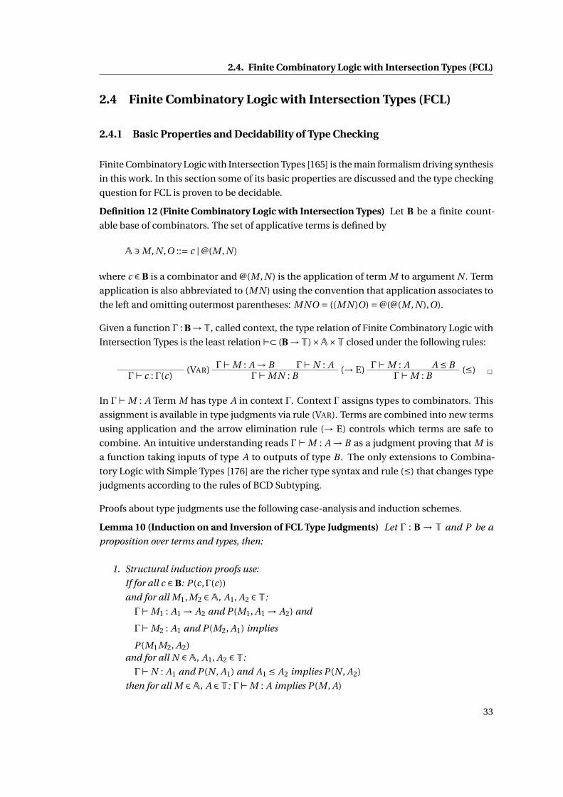
2.4. Finite Combinatory Logic with Intersection Types (FCL)
2.4 Finite Combinatory Logic with Intersection Types (FCL)
2.4.1 Basic Properties and Decidability of Type Checking
Finite Combinatory Logic with Intersection Types [165] is the main formalism driving synthesis
in this work. In this section some of its basic properties are discussed and the type checking
question for FCL is proven to be decidable.
Definition 12 (Finite Combinatory Logic with Intersection Types) Let B be a finite count-
able base of combinators. The set of applicative terms is defined by
A ∋ M , N ,O ::= c | @(M , N )
where c ∈ B is a combinator and @(M , N ) is the application of term M to argument N . Term
application is also abbreviated to (M N ) using the convention that application associates to
the left and omitting outermost parentheses: M NO = ((M N )O) = @(@(M , N ),O).
Given a function Γ : B →T, called context, the type relation of Finite Combinatory Logic with
Intersection Types is the least relation ⊢⊂ (B →T)×A×T closed under the following rules:
(VAR)Γ⊢ c : Γ(c)
Γ⊢ M : A → B Γ⊢ N : A (→ E)Γ⊢ M N : B
Γ⊢ M : A A ≤ B (≤)Γ⊢ M : B □
In Γ⊢ M : A Term M has type A in context Γ. Context Γ assigns types to combinators. This
assignment is available in type judgments via rule (VAR). Terms are combined into new terms
using application and the arrow elimination rule (→ E) controls which terms are safe to
combine. An intuitive understanding reads Γ⊢ M : A → B as a judgment proving that M is
a function taking inputs of type A to outputs of type B . The only extensions to Combina-
tory Logic with Simple Types [176] are the richer type syntax and rule (≤) that changes type
judgments according to the rules of BCD Subtyping.
Proofs about type judgments use the following case-analysis and induction schemes.
Lemma 10 (Induction on and Inversion of FCL Type Judgments) Let Γ : B → T and P be a
proposition over terms and types, then:
1. Structural induction proofs use:
If for all c ∈ B: P (c,Γ(c))
and for all M1, M2 ∈A, A1, A2 ∈T:
Γ⊢ M1 : A1 → A2 and P (M1, A1 → A2) and
Γ⊢ M2 : A1 and P (M2, A1) implies
P (M1M2, A2)and for all N ∈A, A1, A2 ∈T:
Γ⊢ N : A1 and P (N , A1) and A1 ≤ A2 implies P (N , A2)
then for all M ∈A, A ∈T: Γ⊢ M : A implies P (M , A)
33

Chapter 2. Theory
2. Combinator judgments can be reduced to Subtype judgments:
for all c ∈ B, A ∈T: If Γ⊢ c : A then Γ(c) ≤ A
3. Arrow elimination can be inverted:
for all M , N ∈A, B ∈T:
If Γ⊢ M N : B then there exists A, s.t. Γ⊢ M : A → B and Γ⊢ N : A
4. Normalized induction proofs use:
If for all c ∈ B: P (c,Γ(c))
and for all c ∈ B, A ∈T:
P (c,Γ(c)) and Γ(c) ≤ A implies P (c, A)
and for all M1, M2 ∈A, A1, A2 ∈T:
Γ⊢ M1 : A1 → A2 and P (M1, A1 → A2) and
Γ⊢ M2 : A1 and P (M2, A1) implies
P (M1M2, A2)then for all M ∈A, A ∈T: Γ⊢ M : A implies P (M , A)
PROOF
1. Recursion using the fact that trees are finite objects and children get smaller in each
step.
2. Structural induction using the scheme from Lemma 10.1.
3. Structural induction using the scheme from Lemma 10.1.
4. Structural induction using the scheme from Lemma 10.1 and then Lemma 10.2 for the
subtyping case, and Lemma 10.3 arrow elimination case. ■
The formalization is set up such that two more rules are derivable, which are sometimes
explicitly included into the system [50; 165].
Lemma 11 (Rules derivable in FCL) The following two additional rules are derivable in FCL:
Γ⊢ M : A Γ⊢ M : B (∩I)Γ⊢ M : A∩B
(Aω)Γ⊢ M :ω
PROOF Both by structural induction on the derivation. For (∩I) additionally Lemma 10.2 and
Lemma 10.3 are used. The proof for rule (Aω) uses the fact that Γ is represented as a function
and has to assign some type A to every combinator, which then can be converted into an
arrow in case of application using BCD rules (ω) and (→ω): A ≤ω≤ω→ω. ■
The system also allows weakening by making subtype assumptions smaller.
34

2.4. Finite Combinatory Logic with Intersection Types (FCL)
Lemma 12 (Weakening Subtypes) For all Γ1,Γ2 : B →T: if for all c ∈ B: Γ2(c) ≤ Γ1(c) then for
all M ∈A, A ∈T: if Γ1 ⊢ M : A then Γ2 ⊢ M : A.
PROOF By normalized induction (Lemma 10.4) on the derivation Γ1 ⊢ M : A. ■
Many other properties of FCL are best expressed using the construct of multi arrows.
Definition 13 (Multi Arrows) A multi arrow m is a pair T∗×T, where the first component,
srcs, is a list of source types and the second component, tgt, is a target type. Projections m.1
and m.2 select these components.
Multi arrows are converted into types using:
mkArrow(m) = foldl(λt s.s → t )(m.2)(m.1) □
Lemma 13 (Properties of mkArrow) For src, tgt, tgt1, tgt2 ∈T, and srcs,srcs1, srcs2 ∈T∗ func-
tion mkArrow has the following formal properties:
1. mkArrow(([:: src&srcs], tgt)) = last(src,srcs) → mkArrow((srcs, tgt))
2. mkArrow((rcons(srcs,src), tgt)) = mkArrow((srcs,src → tgt))
3. arity(mkArrow((rcons(srcs,src), tgt))) =T×T4. If tgt1 ≤ tgt2 then mkArrow((srcs, tgt1)) ≤ mkArrow((srcs, tgt2))
5. If isOmega(tgt) then isOmega(mkArrow((srcs, tgt)))
6. If tgt ∈Tπ then mkArrow((srcs, tgt)) ∈Tπ7. mkArrow((srcs, tgt1 ∩ tgt2)) ≤ mkArrow((srcs, tgt1))∩mkArrow((srcs, tgt2))
8. If lsize(srcs1) = lsize(srcs2) and for all (src1, src2) in zip(srcs1, srcs2): src1 ≤ src2 then
mkArrow((srcs1, tgt)) ≤ mkArrow((srcs2, tgt))
PROOF In the order presented and by inserting the definition of mkArrow and induction or
induction in reverse order on the source types. ■
There is an analogous operation to mkArrow on the term level.
Definition 14 (Reverse Application) Terms can be constructed from other terms M ∈A, N s ∈A∗ using reverse application:
revApply((M , N s)) = foldr(λN M .@(M , N ))(M)(N s).
The inverse operation is defined by:
unapply(M) =⎧⎨⎩(c, [::]) for M = c
(c, [:: N &N s]) for M = M ′N and unapply(M ′) = (c, N s)
35

Chapter 2. Theory
Lemma 14 (Properties of revApply and unapply) For M , N ∈A, c ∈ B, and N s ∈A∗ functions
revApply and unapply have the following formal properties:
1. revApply((M , rcons(N s, N ))) = revApply((@(M , N ), N s))
2. revApply((M , [::])) = M
3. revApply(unapply(M))) = M
4. unapply(revApply((c, N s)) = (c, N s)
PROOF Inserting definitions and induction. ■
Being able to construct arrows and terms from lists generalizes (inverse) arrow elimination.
Lemma 15 (Generalized (inverse) Arrow Elimination)
Let M ∈ A, N s ∈ A∗, tgt ∈ T, srcs ∈ T∗ and m be a multi arrow, then judgments can be
(de-)constructed using:
1. If lsize(N s) = lsize(m.1) and for all n ∈N: Γ⊢ nth(M , N s,n) : nth(mkArrow(m),m.1,n)
then Γ⊢ revApply((M , N s)) : m.2
2. If Γ⊢ revApply(M , N s) : tgt then there exists srcs ∈T∗, s.t. lsize(N s) = lsize(srcs) and for
all n ∈N: Γ⊢ nth(M , N s,n) : nth(mkArrow((srcs, tgt)),srcs,n)
PROOF By induction on N s, using Lemma 10.3 for the second statement. ■
Moreover, minimal types can now be assigned to any given term M .
Definition 15 (Minimal Types) The minimal type of M ∈A in context Γ : B →T is found by:
minimalType(Γ, M) =⎧⎪⎪⎪⎪⎪⎪⎪⎨⎪⎪⎪⎪⎪⎪⎪⎩
Γ(c) for M = c⋂Ai∈∆ Ai
for M = M ′N and
[ tgt_for_srcs_gte minimalType(Γ, N ) in castω→ω⋆ωminimalType(Γ, M ′)]
↝ [ check_tgt ∆]
where ∆ is computed using Definition 9 with a termination certificate obtained by Lemma 2.□
Lemma 16 (Minimal Type Correctness) Let M ∈ A, A,B ,C ∈ T and Γ : B → T then function
minimalType computes the correct minimal type:
1. For all ∆ in [ tgt_for_srcs_gte B in castω→ω⋆ω A]↝ [ check_tgt ∆]:
A ≤ B →⋂Ai∈∆ Ai
36

2.4. Finite Combinatory Logic with Intersection Types (FCL)
2. Γ⊢ M : minimalType(Γ, M)
3. If A ≤ B →C then
for all ∆ in [ tgt_for_srcs_gte B in castω→ω⋆ω A]↝ [ check_tgt ∆]:⋂Ai∈∆ Ai ≤C
4. If Γ⊢ M : A then minimalType(Γ, M) ≤ A
PROOF The intermediate statements 1 and 3 are proven by analysis of the last step of the
subtype machine, and each time two separate cases for the result of isOmega(B), showing
that castω→ω⋆ω will find appropriate targets. Soundness in statement 2 is shown by structural
induction using previous case 1 for (→ E). Minimality in statement 4 is shown by normalized
induction using the previous statements 3 for (→ E). ■
Minimal type inference and decidability of the BCD relation are enough to provide a type-
checking algorithm for FCL.
Theorem 3 (Type Checking in FCL) Let M ∈A, A ∈T and Γ : B →T then
Γ⊢ M : A iff minimalType(Γ, M) ≤ A
PROOF The forward direction of the iff is minimality from Lemma 16.4, the other direction
follows from soundness Lemma 16.2 and rule (≤). ■
The rest of this section is dedicated to the study of type inhabitation. The algorithm to infer
minimal types solves the problem: Given a context Γ, and a term M , find the minimal type,
such that Γ⊢ M : A is derivable. Type inhabitation solves the same problem for terms: Given a
context Γ and type A, find all terms M such that Γ⊢ M : A is derivable.
2.4.2 Combining Separate Domains of Discourse
Finite Combinatory Logic with Intersection Types has the power to reason about multiple
domains of discourse simultaneously. Sometimes these domains are hard to describe in a
technically precise way. Steffen et al. [181] have introduced taxonomic modeling with semantic
type descriptors in the setting of synthesis. This was later adopted for intersection types and
inhabitation based synthesis [163]. Successful applications have been demonstrated multiple
times in various different scenarios [57; 59; 20; 21; 23; 96; 25; 171; 201]. Yet, with the notable
exception of [59] where the type system was modified to separate semantic domains, no formal
study has been conducted on mathematical conditions that make a separation of domains of
discourse possible. At this point, enough theory has been established to illustrate semantic
types and domain separation by example.
37

Chapter 2. Theory
Example 1 (Semantic Types) Suppose synthesis is used to create sheets for the music running
in background to motivate reading or writing this text. The sheet is typeset by LilyPond [143],
which can process a textual markup language. One combinator, addLyrics, inserts lyrics
text into a LilyPond markup file. Another combinator, motivationSong, provides a markup
file of "No Surrender" by Bruce Springsteen. Imagine that an automated web search has
downloaded lyrics including the text "surrender" and two combinators have been created.
The first combinator, noSurrender, provides the correct lyrics. The second combinator,
ISurrender, provides the lyrics of "I Surrender" by Celine Dion.
In a technical domain of discourse these combinators can be typed as follows:
Γ1 = { addLyrics : LilyPond(Music) → String → LilyPond(Song)
motivationSong : LilyPond(Music)
noSurrender : String
ISurrender : String }
Synthesis in the technical domain uses type inhabitation to create all terms for which type
LilyPond(Song) is derivable, i.e. the set
{ addLyrics motivationSong noSurrender,
addLyrics motivationSong ISurrender }.
The first term represents the correct version with the advice "No retreat baby, no surrender"
[177]. However the second term not only has a text out of tune, but also includes the disastrous
advice "I surrender. Every night’s getting longer" [51].
A different, nontechnical, domain of discourse describes artist information:
Γ2 = { addLyrics : (Springsteen → Springsteen → Springsteen)∩(Dion → Dion → Dion)
motivationSong : Springsteen
noSurrender : Springsteen
ISurrender : Dion }.
In this domain the type of combinator addLyrics forces the music and lyrics artist of its
arguments to match.
38

2.4. Finite Combinatory Logic with Intersection Types (FCL)
The inhabitants of type Springsteen are
{ motivationSong,
noSurrender,
addLyrics motivationSong noSurrender,
addLyrics noSurrender motivationSong,
addLyrics (addLyrics motivationSong noSurrender) motivationSong,
addLyrics motivationSong (addLyrics motivationSong noSurrender), . . . }.
The problematic use of advice from Celine Dion is avoided, but an infinite set of solutions is
found. The output of addLyrics is fed back as input. Moreover, compared to the technical
domain, the arguments of addLyrics are in the wrong order in some terms.
This section discusses why it is correct (sound and complete) to combine Γ1 and Γ2 into
Γ3(c) = Γ1(c)∩Γ2(c), for which inhabitation of LilyPond(Song)∩Springsteen exactly yields the
correct answer
{addLyrics motivationSong noSurrender}.
□
Types in combined contexts need to be classified according to their provenance. The following
definitions make this classification mathematically precise.
Definition 16 (Split Type Universes) A Boolean predicate inPartition :T→B is called proper
classifier, if for all A,B ∈T the following conditions are satisfied:
1. inPartition(A → B) iff inPartition(A) and inPartition(B)
2. inPartition(A∩B) iff inPartition(A) and inPartition(B)
3. inPartition(ω) = true
Two classifiers inPartition1, inPartition2 :T→B are disjoint, if for all A,B ,C ∈T:
1. If inPartition1(A), inPartition2(B), inPartition1(C ), and A∩B ≤C then A ≤C
2. If inPartition2(A), inPartition1(B), inPartition2(C ), and A∩B ≤C then A ≤C
A Split Type Universe is a pair of proper disjoint classifiers. □
Definition 17 (Split Context Pairs) Let (inPartition1, inPartition2) be a Split Type Universe.
The pair of contexts Γ1,Γ2 : B →T is a Split Context Pair, if for all c ∈ B:
inPartition1(Γ1(c)) and inPartition2(Γ2(c)) □
39

Chapter 2. Theory
Lemma 17 (Properties of Split Context Pairs) For all Split Context Pairs (Γ1,Γ2) over a Split
Type Universe (inPartition1, inPartition2), and A,B ∈ T, ∆ ∈ T∗, and M , N ∈ A, the following
statements are true:
1. inPartition1(⋂
Ai∈∆ Ai ) iff for all A in ∆: inPartition1(A)
2. inPartition2(⋂
Ai∈∆ Ai ) iff for all A in ∆: inPartition2(A)
3. inPartition1(minimalType(Γ1, M))
4. inPartition2(minimalType(Γ2, M))
5. There exist ∆1,∆2 ∈T∗, s.t.
minimalType(Γ1, M) =⋂Ai∈∆1
Ai and minimalType(Γ2, M) =⋂Ai∈∆2
Ai and
for Γ(c) = Γ1(c)∩Γ2(c): minimalType(Γ, M) =⋂Ai∈∆1++∆2
Ai
PROOF Statements 1 and 2 are proven by induction on∆. Statements 3 and 4 require induction
on M , and in the case for applications M = M ′N additional induction on minimalType(Γi , M ′)with index i selecting the context mentioned in the statement to show. The last statement is
shown by induction on M and ∆1,∆2 are [::Γ1(c)], [::Γ2(c)] for M = c or the type lists ∆ used in
the minimalType algorithm for the case of M = M ′N . In the latter case a detailed analysis of
subtype machine behavior is required. ■
Theorem 4 (Split Context Pair Correctness) For all Split Context Pairs (Γ1,Γ2) over a Split
Type Universe (inPartition1, inPartition2), and A,B ∈T, M ∈A, and Γ(c) = Γ1(c)∩Γ2(c):
If inPartition1(A) and inPartition2(B) then
Γ⊢ M : A∩B iff Γ1 ⊢ M : A and Γ2 ⊢ M : B.
PROOF Combining proofs Γ1 ⊢ M : A and Γ2 ⊢ M : B into Γ⊢ M : A∩B is possible because of
Lemma 11 rule (∩) and the context weakening property from Lemma 12. The other direction
follows from the minimality and soundness in Lemma 16, Lemma 17.5, disjointness of universe
classifiers, as well as Lemma 17.3 and Lemma 17.4. ■
In fact, any context pair (Γ1,Γ2) can be transformed into a Split Context Pair. The transforma-
tion requires a theory of intersection homomorphisms and their effect as context transforma-
tions in FCL.
Definition 18 (Intersection Type Homomorphism) Let C1,C2 be preordered countable sets
of constructor symbols and T1,T2 types formed over each of these sets. Function f :T1 →T2
is an Intersection Type Homomorphism if it satisfies the following conditions for arbitrary
types A,B ∈T1:
1. A ≤ B iff f (A) ≤ f (B)
40
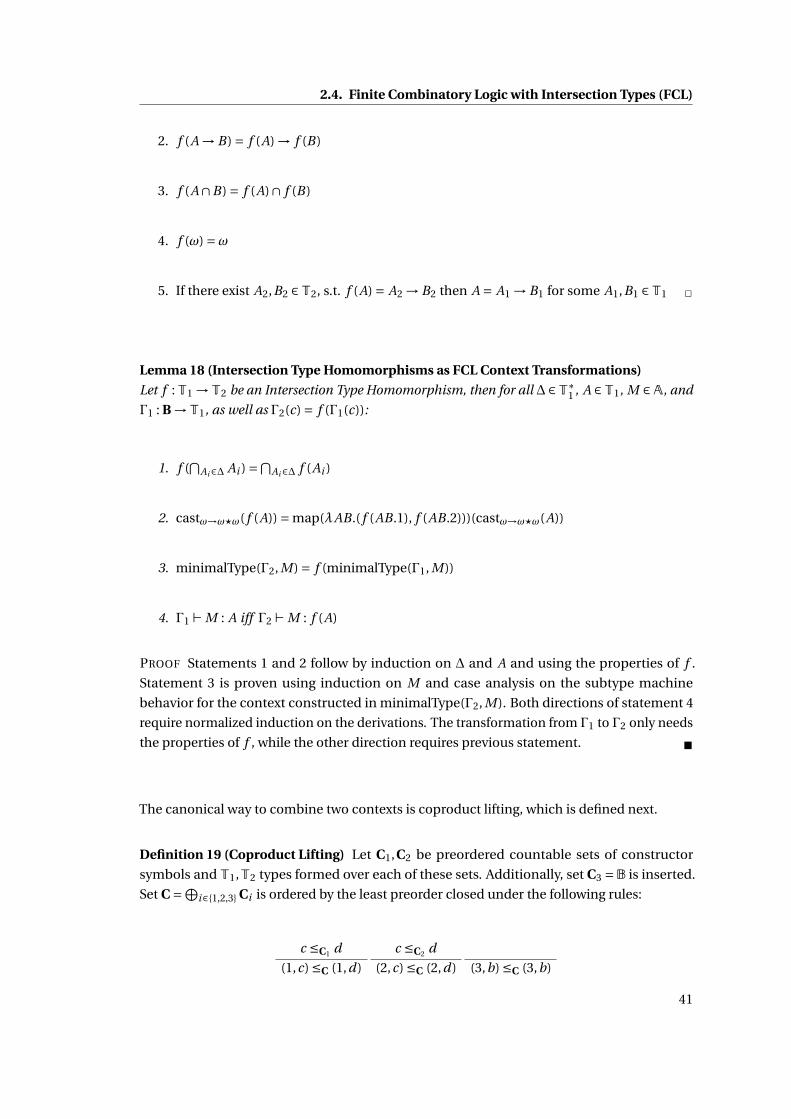
2.4. Finite Combinatory Logic with Intersection Types (FCL)
2. f (A → B) = f (A) → f (B)
3. f (A∩B) = f (A)∩ f (B)
4. f (ω) =ω
5. If there exist A2,B2 ∈T2, s.t. f (A) = A2 → B2 then A = A1 → B1 for some A1,B1 ∈T1 □
Lemma 18 (Intersection Type Homomorphisms as FCL Context Transformations)
Let f :T1 →T2 be an Intersection Type Homomorphism, then for all ∆ ∈T∗1 , A ∈T1, M ∈A, and
Γ1 : B →T1, as well as Γ2(c) = f (Γ1(c)):
1. f (⋂
Ai∈∆ Ai ) =⋂Ai∈∆ f (Ai )
2. castω→ω⋆ω( f (A)) = map(λAB.( f (AB.1), f (AB.2)))(castω→ω⋆ω(A))
3. minimalType(Γ2, M) = f (minimalType(Γ1, M))
4. Γ1 ⊢ M : A iff Γ2 ⊢ M : f (A)
PROOF Statements 1 and 2 follow by induction on ∆ and A and using the properties of f .
Statement 3 is proven using induction on M and case analysis on the subtype machine
behavior for the context constructed in minimalType(Γ2, M). Both directions of statement 4
require normalized induction on the derivations. The transformation from Γ1 to Γ2 only needs
the properties of f , while the other direction requires previous statement. ■
The canonical way to combine two contexts is coproduct lifting, which is defined next.
Definition 19 (Coproduct Lifting) Let C1,C2 be preordered countable sets of constructor
symbols and T1,T2 types formed over each of these sets. Additionally, set C3 =B is inserted.
Set C =⨁i∈{1,2,3} Ci is ordered by the least preorder closed under the following rules:
c ≤C1 d
(1,c) ≤C (1,d)
c ≤C2 d
(2,c) ≤C (2,d) (3,b) ≤C (3,b)
41

Chapter 2. Theory
Coproduct lifting into types T formed over C is perfomed using:
lift1(A) = lift(liftCtor1, true, A)
lift2(A) = lift(liftCtor2, false, A)
liftCtor1(A) = (1, A)
liftCtor2(A) = (2, A)
lift(liftCtor, isLeft, A) =⎧⎪⎪⎪⎪⎪⎪⎪⎪⎪⎨⎪⎪⎪⎪⎪⎪⎪⎪⎪⎩
ω for A =ωliftCtor(c)(lift(liftCtor, isLeft,B)) for A = c(B)
lift(liftCtor, isLeft, A1) → lift(liftCtor, isLeft, A2) for A = A1 → A2
(3, isLeft)(lift(liftCtor, isLeft, A1)⋆ lift(liftCtor, isLeft, A2)) for A = A1⋆ A2
lift(liftCtor, isLeft, A1)∩ lift(liftCtor, isLeft, A2) for A = A1 ∩ A2
Coproduct lifting has partially defined right inverses:
unlift(unliftCtor, A) =⎧⎪⎪⎪⎪⎪⎪⎪⎪⎪⎪⎪⎪⎪⎪⎪⎪⎪⎪⎪⎪⎪⎪⎪⎪⎪⎪⎪⎪⎨⎪⎪⎪⎪⎪⎪⎪⎪⎪⎪⎪⎪⎪⎪⎪⎪⎪⎪⎪⎪⎪⎪⎪⎪⎪⎪⎪⎪⎩
ω for A =ωA′
1⋆ A′2 for A = (3,b)(A1, A2) and
unlift(unliftCtor, A1) = A′1 and
unlift(unliftCtor, A2) = A′2
c ′(B ′) for A = (i ,c)(B) and i ∈ {1,2} and
unliftCtor((i ,c)) = c ′ and
unlift(unliftCtor,B) = B ′
A′1 → A′
2 for A = A1 → A2 and
unlift(unliftCtor, A1) = A′1 and
unlift(unliftCtor, A2) = A′2
A′1 ∩ A′
2 for A = A1 ∩ A2 and
unlift(unliftCtor, A1) = A′1 and
unlift(unliftCtor, A2) = A′2
unliftCtor1(c) = c ′for c = (1,c ′)
unliftCtor2(c) = c ′for c = (2,c ′)
unlift1(A) = unlift(unliftCtor1, A)
unlift2(A) = unlift(unliftCtor2, A)
42

2.4. Finite Combinatory Logic with Intersection Types (FCL)
There is an easy to define pair of T-classifiers inPartition j for j ∈ {1,2}:
inPartition j (A) =⎧⎪⎪⎪⎪⎪⎪⎪⎪⎪⎪⎪⎨⎪⎪⎪⎪⎪⎪⎪⎪⎪⎪⎪⎩
true for A =ωtrue for A = (i ,c)(B) and i = j and inPartition j (B)
true for A = (3, true)(A1⋆ A2) and j = 1 and inPartition j (A1) and inPartition j (A2)
true for A = A1 → A2 and inPartition j (A1) and inPartition j (A2)
true for A = A1 ∩ A2 and inPartition j (A1) and inPartition j (A2)
false otherwise
□
The lifting is mostly straight-forward, except for the subtle encoding of products. The latter is
necessary to prevent information leakage between type universes from nested products. Type
ω⋆ω illustrates this point: it contains information because ω≤ω⋆ω is false, but without the
product encoding it cannot be uniquely classified as belonging to any type universe.
Lemma 19 (Properties of Coproduct Lifting) Again let C1,C2 be preordered countable sets of
constructor symbols, T1,T2 types formed over each of these sets and T be formed over C as
constructed in Definition 19. For all k ∈ {1,2}, (ck ,dk ∈ Ck ), and Ak , A1k , A2
k ∈Tk , ∆k ∈T∗k , and
B ,B1,B2 ∈T, c ∈ C, b1 = true, b2 = false, coproduct lifting has the following properties:
1. liftk (A1k → A2
k ) = liftk (A1k ) → liftk (A2
k )
2. liftk (A1k ∩ A2
k ) = liftk (A1k )∩ liftk (A2
k )
3. If there exists A′1, A′
2, s.t. liftk (Ak ) = A′1 → A′
2 then
there exists A1, A2 ∈Tk , s.t. Ak = A1 → A2
4. liftk (ω) =ω
5. unliftk (liftk (Ak )) = Ak
6. liftk (⋂
Ai∈∆kAi ) =⋂
Ai∈map(λA. liftk (A))(∆k ) Ai
7. castliftk (ck (Bk ))(liftk (Ak )) = map(λA. liftk (A))(castck (Bk )(Ak ))
8. isOmega(Ak ) = isOmega(liftk (Ak ))
9. castliftk (A1k→A2
k )(liftk (Ak )) = map(λAB.(liftk (AB.1), liftk (AB.2)))(castA1k→A2
k(Ak ))
10. castliftk (A1k⋆A2
k )(liftk (Ak )) = map(λAB.(liftk (AB.1), liftk (AB.2)))(castA1k⋆A2
k(Ak ))
11. If B = liftk (A1k )⋆ liftk (A2
k ) and ∆= cast(3,bk )(B)(liftk (Ak )) then
castB (⋂
Ai∈∆ Ai ) = map(λAB.(liftk (AB.1), liftk (AB.2)))(castA1k⋆A2
kAk )
43

Chapter 2. Theory
12. A1k ≤ A2
k iff liftk (A1k ) ≤ liftk (A2
k )
13. inPartitionk (liftk (Ak )) = true
14. inPartitionk (B1 → B2) = inPartitionk (B1) and inPartitionk (B2)
15. inPartitionk (B1 ∩B2) = inPartitionk (B1) and inPartitionk (B2)
16. inPartitionk (ω) = true
17. If inPartition1(B1) and inPartition2(c(B2)) then castc(B2)(B1) = [::]
If inPartition2(B1) and inPartition1(c(B2)) then castc(B2)(B1) = [::]
18. If inPartition1(B1) and inPartition2(B2) and B1 ≤ B2 then isOmega(B2)
If inPartition2(B1) and inPartition1(B2) and B1 ≤ B2 then isOmega(B2)
19. If inPartitionk (B) then for all B ′ in primeFactors(B): inPartitionk (B ′)
20. If inPartition1(B1) and inPartition2(B2) and inPartition1(B) and B1 ∩B2 ≤ B then B1 ≤ B
If inPartition1(B1) and inPartition2(B2) and inPartition2(B) and B1 ∩B2 ≤ B then B2 ≤ B
PROOF The statements are proven in the order presented. Most follow from simple induction,
previous lemmas and unfolding of definitions. Statements 12 and 16 require analyzing the
operational semantics of the subtype machine and induction on the termination certificates
for [ subty A1k of A2
k ] and [ subty B1 of B2]. This is necessary because of transitivity
and the change of arrow variance. For similar reasons, statement 19 is proven by induction in
the size of B . Statement 20 is proven using statement 19 and correctness of prime factorization
(Theorem 2). ■
Theorem 5 (Coproduct Lifting Context Pairs to Split Context Pairs) Any pair of contexts Γ1 :
B → T1 and Γ2 : B → T2 can be lifted into Γ′1(c) = lift1(Γ1(c)) and Γ′2(c) = lift2(Γ2(c)) and
combined to Γ(c) = Γ′1(c)∩Γ′2(c) such that for all A ∈T1, B ∈T2, and M ∈A:
Γ⊢ M : lift1(A)∩ lift2(B) iff Γ1 ⊢ M : A and Γ2 ⊢ M : B.
PROOF By Lemma 19, inPartition1 and inPartition2 are proper disjoint classifiers and (Γ′1,Γ′2)
is a Split Context Pair. Also by Lemma 19, lift1 and lift2 are Intersection Type Homomorphisms.
Hence type judgments of the lifted contexts can be transformed back and forth between the
original and lifted contexts by Lemma 18. ■
44

2.5. Verified Enumerative Type Inhabitation in FCL
2.5 Verified Enumerative Type Inhabitation in FCL
This section discusses an algorithm for enumerative type inhabitation (enumerate all inhabi-
tants of a given type) in FCL. Rehof and Urzyczyn [165] have studied the decision problem for
type inhabitation in FCL and characterized it as EXPTIME-complete. The decision problem be-
comes undecidable if the system is extended with schematism and (1+k)-EXPTIME-complete1
if the schematism is restricted to variable instantiations of maximal depth k [57]. The decision
problem (does there exist an inhabitant of a given type?) is informative for complexity theory
and [165] also provides decision procedures for the problems of ambiguity (do there exist
multiple inhabitants of a given type?) and infinity (do there exist infinitely many inhabi-
tants of a given type?). Decidability and the alternating tree-automaton based representation
of FCL without subtyping [165] inform the design of an enumerative type inhabitation al-
gorithm, which can construct inhabitants instead of just answering questions about their
existence. The enumerative approach is most valuable from the practical perspective of soft-
ware synthesis and has been at the heart of multiple implementations of the (CL)S Framework
[56; 59; 55; 20; 61]. Yet, it has never been formalized – a gap that has existed for almost 10 years
of development and is finally closed in this section.
2.5.1 The Cover Machine
Combinators are the building blocks of FCL and the most fundamental task in any type
inhabitation algorithm is: given a combinator and a target type, find (all) possible types of
arguments, such that application of the combinator produces (covers) the desired target. The
cover machine solves this goal. For its specification some auxiliary functions are necessary.
Definition 20 (Auxiliary functions for the cover machine) Subtype duplicate free intersec-
tion is defined by:
A ⋔B =
⎧⎪⎪⎪⎨⎪⎪⎪⎩A for A ≤ B
B for not A ≤ B and B ≤ A
A∩B otherwise
Function partitionCover partitions a list of types according to membership in another list:
partitionCover(∆1,∆2) =
⎧⎪⎪⎪⎪⎪⎪⎪⎪⎨⎪⎪⎪⎪⎪⎪⎪⎪⎩
([::], [::]) for ∆2 = [::]
([:: A&∆12],∆2
2) for ∆2 = [:: A&∆] and A in ∆1 and
partitionCover(∆1,∆) = (∆12,∆2
2)
(∆12, [:: A&∆2
2]) for ∆2 = [:: A&∆] and not A in ∆1 and
partitionCover(∆1,∆) = (∆12,∆2
2)
1The definition of depth(A) in this text coincides with level(A)+1 in [57].
45

Chapter 2. Theory
Predicate stillPossible : (((T∗×T)×T∗)∗×T∗) → B tests for a list of multi arrows with target
components they cover and a list of target components, which are yet to cover, if these still
can be covered:
stillPossible(splits, toCover) = for all A in toCover :
exists covered ∈ map(λmCovered.mCovered.2)(splits) :
A ∈ covered
Function mergeMultiArrow distributes duplication free intersection over two multi arrows:
mergeMultiArrow(m1,m2) = (map(λsrcs.srcs.1⋔ srcs.2)(zip(m1.1,m2.1)),m1.2⋔m2.2)
Definition 21 (Cover Machine) The instructions of the cover machine are given by
ICover ∋ i ::= Cover splits toCover
| CheckCover splits toCover
| ContinueCover splits toCover currentResult
| CheckContinueCover splits toCover currentResult
where
• splits ∈ ((T∗×T)×T∗)∗ is a list of multi arrows with parts of the target they cover
• toCover ∈T∗ is a list of target components still to cover
• currentResult ∈T∗×T is an intermediate multi arrow, possibly added to the result
The output OCover = (T∗×T)∗ is a list of multi arrows.
Behavior of the cover machine is specified by the following step relation:
not stillPossible(splits, toCover)(STEPCHECKPRUNE)
(s, [:: CheckCover splits toCover&p])↝ (s, p)
not stillPossible(splits, toCover)(STEPCHECKCONTINUEPRUNE)
(s, [:: CheckContinueCover splits toCover currentResult&p])↝ (s, p)
stillPossible(splits, toCover)(STEPCHECKOK)
(s, [:: CheckCover splits toCover&p])↝ (s, [:: Cover splits toCover&p])
stillPossible(splits, toCover)(STEPCHECKCONTINUEOK)
(s, [:: CheckContinueCover splits toCover currentResult&p])↝
(s, [:: ContinueCover splits toCover currentResult&p])
(STEPDONE)(s, [:: Cover [::] toCover&p])↝ (s, p)
46

2.5. Verified Enumerative Type Inhabitation in FCL
(STEPDONECONTINUE)(s, [:: ContinueCover [::] toCover currentResult&p])↝ (s, p)
partitionCover(covered,toCover) = ([::],∆)(STEPSKIP)
(s, [:: Cover [:: (m,covered)&splits] toCover&p])↝ (s, [:: Cover splits toCover&p])
partitionCover(covered,toCover) = ([::],∆)(STEPSKIPCONTINUE)
(s, [:: ContinueCover [:: (m,covered)&splits] toCover currentResult&p])↝
(s, [:: ContinueCover splits toCover currentResult&p])
partitionCover(covered,toCover) = ([:: A&∆], [::])(STEPADDDONE)
(s, [:: Cover [:: (m,covered)&splits] toCover&p])↝
([:: m&s], [:: CheckCover splits toCover&p])
partitionCover(covered,toCover) = ([:: A&∆], [::])(STEPMERGEDONE)
(s, [:: ContinueCover [:: (m,covered)&splits] toCover currentResult&p])↝
([:: mergeMultiArrow(currentResult,m)&s],
[:: CheckContinueCover splits toCover currentResult&p])
partitionCover(covered,toCover) = ([:: A&∆1], [:: B&∆2])(STEPCONTINUE)
(s, [:: Cover [:: (m,covered)&splits] toCover&p])↝
(s, [:: ContinueCover splits [:: B&∆2] m&[:: CheckCover splits toCover&p]])
partitionCover(covered,toCover) = ([:: A&∆1], [:: B&∆2])
mergeMultiArrow(currentResult,m).1 = currentResult.1 (STEPCONTINUE-
MERGEALWAYS
)
(s, [:: ContinueCover [:: (m,covered)&splits] toCover currentResult&p])↝
(s, [:: ContinueCover splits [:: B&∆2]mergeMultiArrow(currentResult,m)&p])
partitionCover(covered,toCover) = ([:: A&∆1], [:: B&∆2])
not mergeMultiArrow(currentResult,m).1 = currentResult.1(STEP
CONTINUE-
MERGE-
OPTIONS
)
(s, [:: ContinueCover [:: (m,covered)&splits] toCover currentResult&p])↝
(s, [:: ContinueCover splits [:: B&∆2]mergeMultiArrow(currentResult,m)&
[:: CheckContinueCover splits toCover currentResult&p]])
The n-step closure of ↝ is the least relation closed under the rules:
(s, p)↝0 (s, p)
1 (s1, p1)↝ (s2, p2) 2 (s2, p2)↝n (s3, p3)
(s1, p1)↝n+1 (s3, p3)
By definition the n-step closure coincides with transtive reflexive closure: (s, p)↝∗ (s′, p ′) iff
there exists n, s.t. (s, p)↝n (s′, p ′). In proof trees t for (s, p)↝n+1 (s′, p ′) the first and second
premise are selected using t .1 and t .2. □
47

Chapter 2. Theory
The cover machine processes a stack of instructions. Results are pushed onto an output stack.
Each of the instructions has lists splits, and toCover. For the initial instructions toCover will be
chosen as the prime factors of the target type. List splits will include multi arrows computed
from the type of a combinator. Each of these multi arrows will have the same number of
arguments and be paired with the target prime factors that are greater or equal than the
multi arrow target. For example, if a combinator x has type Γ(x) = (a → b → c ∩d)∩ (d →e) ∩ ( f → g → h) and the target type is h ∩ c, then one of the initial instructions will be
CheckCover [:: (([:: b&[::a]],c ∩d), [::c])&[::(([:: g &[:: f ]],h), [::h])]] [:: h&[::c]]. This instruction
checks the multi arrows with two targets, which are ([:: b&[::a]],c ∩ d) for a → b → c ∩ d
and ([:: g &[:: f ]],h) for f → g → h. The target prime factors are c and h, so the first multi
arrow is only paired with c, because c ∩d ≤ c and not c ∩d ≤ h. The second multi arrow
is paired with h because h ≤ h and not h ≤ c. Two of the four cover machine instructions
are prefixed with CHECK. They try to prune its exponentially large search space. If at some
point all of the covered components in splits are no longer enough to cover all components
in toCover, the search is aborted and the instruction can be dropped. This shortcut, or
if not viable the resumption of normal operations, is implemented by the first four rules
(STEPCHECKPRUNE), (STEPCHECKCONTINUEPRUNE), (STEPCHECKOK), and (STEPCHECKCONTINUEOK). Rules
(STEPDONE) and (STEPDONECONTINUE) implement failure modes and skip the current instruction.
They are inserted to ensure left totality of the step relation and invariants established for
proper initialization will later prevent, that their precondition (empty choices for splits) ever
occurs. If the first multi arrow in splits does not cover any new elements of toCover, it is
removed by (STEPSKIP) or (STEPDONECONTINUE). The opposite condition, if the first multi arrow
covers all remaining targets, is implemented in rules (STEPADDDONE) and (STEPMERGEDONE). In
each case the multi arrow from splits is pushed to the output stack. In (STEPMERGEDONE) it is also
merged with the current result. When merging two multi arrows, all of their targets and all of
their sources are intersected, avoiding redundancy whenever possible: mergeMultiArrow(([::
b&[::a]],c), ([:: d&[::a ∩ e]], f )) = ([:: b ∩d&[::a ∩ e]],c ∩ f ) where redundancy in the second
argument has been removed, i.e. a ∩e instead of a ∩ (a ∩e). The DONE-rules continue with
the rest of the multi arrows in splits. Intuitively in (a → c)∩ (b → c), type a → c is enough
to cover target c, but b → c is also viable, and recursive targets a and b can have different
inhabitants. Possibilities to cover the target are lost when resuming with the rest of splits, so
prune checks are scheduled. The CONTINUE-rules are used for the remaining cases, where
the first multi arrow in splits covers some, but not all, of the targets in toCover. This multi
arrow is then included in the current result, either by copying it if there was no prior result
(rule (STEPCONTINUE)) or by merging it with the previous result. In rule (STEPCONTINUE) merging
with the previous result does not change any of the sources of the current result. Unlike the
other CONTINUE-rules and the DONE-rules, which need to consider inclusion and exclusion
of the first multi arrow, the multi arrow can always be included in this case. For example in
(a → b)∩ (a → c)∩ (d → e ∩c) with target b∩c ∩e choosing a → c after b → c does not change
any sources ((mergeMultiArrow(([::a],b), ([::a],c))).1 = ([::a],b).1). Unchanged sources imply
that no inhabitants are ruled out for recursive targets compared to the scenario without that
particular choice. The choice is always safe, again avoiding exploration of an entire search
48

2.5. Verified Enumerative Type Inhabitation in FCL
space area.
The first fact to establish about the specification in Definition 21 is functionality (c.f. Lemma 1).
Lemma 20 (Functionality) For all n ∈N, and s, s1, s2 ∈OCover and p, p1, p2 ∈ I∗Cover the cover
machine step relation is functional:
1. If (s, p)↝ (s1, p1) and (s, p)↝ (s2, p2) then (s1, p1) = (s2, p2)
2. If (s, p)↝n (s1, p1) and (s, p)↝n (s2, p2) then (s1, p1) = (s2, p2)
PROOF The precondition of all rules in Definition 21 are mutually exclusive. ■
Definition 22 (Cover Machine Step Function) The result (s′, p ′) of steps (s, p)↝n (s′, p ′) for
n ≤ 1 is computed by:
step(s, p) : {(s′, p ′) ∈ (OCover × I∗Cover) | if p = [::] then (s′, p ′) = (s, p) else (s, p)↝ (s′, p ′)}
step(s, p) =⎧⎪⎨⎪⎩(s, [::]) for p = [::]
(s′, p ′) forP (s, p)
(s, p)↝ (s′, p ′)in the rules of ↝ and P (s, p) = true
Similar to the implementation of the subtype machine, totality of the implementation of the
cover machine is guaranteed by a termination certificate.
Definition 23 (Cover Machine Termination Certificate) For any input (s, p) ∈OCover × I∗Cover
termination certificate Dom(s, p) is a proof tree constructed from the rules of (s, p)↝n (s′, [::])
for some n ∈N and s′ ∈OCover. □
A tail recursive procedure now implements the full n-step behavior of the cover machine.
Definition 24 (Procedure implementing the Cover Machine)
coverMachine(s, p) : Dom(s, p) → {s′ ∈OCover | (s, p)↝∗ (s′, [::])}
coverMachine(s, p)(d) =⎧⎨⎩s′ for step(s, p) = (s′, [::])
coverMachine(s′, [:: i &p ′])(d .2) for step(s, p) = (s, [:: i &p ′])
□
It remains to show that the cover machine is total, i.e. that a termination certificate can be
provided for all inputs.
49

Chapter 2. Theory
Lemma 21 (Totality of the Cover Machine) For i ∈ ICover define:
splitsOf(i ) =⎧⎪⎪⎪⎪⎪⎪⎨⎪⎪⎪⎪⎪⎪⎩
splits for i = Cover splits toCover
or i = CheckCover splits toCover
or i = ContinueCover splits toCover currentResult
or i = CheckCover splits toCover currentResult
isChecked(i ) =⎧⎪⎪⎪⎨⎪⎪⎪⎩true for i = Cover splits toCover
or i = ContinueCover splits toCover currentResult
false otherwise
measure(i ) =⎧⎨⎩22·lsize(splitsOf(i )) for isChecked(i ) = true
22·lsize(splitsOf(i )) +1 otherwise
For all n ∈N, s1, s2 ∈OCover and p1, p2 ∈ I∗Cover the following statements are true:
1. If (s1, p1)↝ (s2, p2) then∑
i in p1measure(i) <∑
i in p2measure(i)
2. If (s1, p1)↝n (s2, p2) then n ≤∑i in p1
measure(i)
3. Proof tree Dom(s1, p1) exists
PROOF The first statement is proven by case analysis on the possibilities for (s1, p1)↝ (s2, p2)
and application of some simple arithmetic. The second statement then follows by induction
on n, the first statement, and transitivity of ≤ on natural numbers. Finally the proof tree
for Dom(s1, p1) is constructed by iterating the single step function up to∑
i in p1measure(i)
times. The second statement proves that more iterations cannot result in additional steps and
thereby the program instruction stack p must be empty as is required for the leaves of the
Dom proof tree. ■
Correctness of the cover machine is a multi faceted issue and its proof requires to study
multiple properties and invariants of the machine behavior first.
Lemma 22 (Stack Behavior) For all s1, s2 ∈OCover, and p1, p2 ∈ I∗Cover the cover machine satis-
fies the following stack invariants for its state and list of instructions
1. If (s1, p1)↝ (s2, p2) then suffix(behead(p1), p2)
2. If (s1, p1)↝ (s2, p2) then suffix(s1, s2)
3. If (s1, p1)↝∗ (s2, p2) then suffix(s1, s2)
PROOF Case analysis and in the last case induction on the steps. ■
50

2.5. Verified Enumerative Type Inhabitation in FCL
More auxiliary functions for multi arrows are used in the subsequent specifications.
Definition 25 (Auxiliary Functions for Multi Arrows) Function mergeMultiArrows merges se-
quences of multi arrows:
mergeMultiArrows(ms) =⎧⎨⎩([::],ω) for ms = [::]
foldl(λm1m2.mergeMultiArrow(m1,m2))(m)(ms′) for ms = [:: m&ms′]
Function filterMergeMultiArrows flattens sequences of sequences of multi arrows by merging
subsequences or removing them if they are empty:
filterMergeMultiArrows(mss) =⎧⎪⎪⎪⎪⎪⎨⎪⎪⎪⎪⎪⎩[::] for mss = [::]
filterMergeMultiArrows(mss′) for mss = [:: [::]&mss′]
[:: mergeMultiArrows([:: m&ms])&
filterMergeMultiArrows(mss′)]
for mss = [:: [:: m&ms]&mss′]
Components that might be subject to merging in a run of the cover machine are collected
from its instructions using:
mergeComponentsOf(i ) =⎧⎪⎪⎪⎪⎪⎪⎪⎪⎪⎪⎨⎪⎪⎪⎪⎪⎪⎪⎪⎪⎪⎩
map(λm.m.1)(splits)
for i = Cover splits toCover or
i = CheckCover splits toCover
[:: currentResult&map(λm.m.1)(splits)]
for i = ContinueCover splits toCover currentResult or
i = CheckContinueCover splits toCover currentResult
□
The first soundness property captures the fact that the cover machine does not add multi
arrows to its results which were not present in its input instructions:
Lemma 23 (Cover Machine Input Merge Component Soundness)
For mss1,mss2 ∈ ((T∗×T)∗)∗, and m1,m2 ∈ (T∗×T), i ∈ ICover, and p1, p2 ∈ I∗Cover, and s1, s2 ∈OCover, and splits ∈ ((T∗×T)×T∗)∗ the following statements are true:
1. filterMergeMultiArrows(mss1 ++mss2) =filterMergeMultiArrows(mss1)++filterMergeMultiArrows(mss2)
2. If mss1 ⊑ mss2 then filterMergeMultiArrows(mss1) ⊑ filterMergeMultiArrows(mss2)
51

Chapter 2. Theory
3. filterMergeMultiArrows(map(λms.[:: mergeMultiArrow(m1,m2)&ms])(mss1)) =filterMergeMultiArrows(map(λms.[:: m1&[:: m2&ms]])(mss1))
4. If (s1, [:: i &p1])↝ (s2, p2) then
for all m in take(lsize(s2)− lsize(s1), s2) :
m is in filterMergeMultiArrows(subseqs(mergeComponentsOf(i )))
Define soundness as a Boolean predicate on OCover × I∗Cover by:
sound(s, p) = for all m in s :
m is in
flatten(map(λi .filterMergeMultiArrows(subseqs(mergeComponentsOf(i ))))(p))
5. If (s1, p1)↝ (s2, p2) then sound(take(lsize(s2)− lsize(s1), s2), p1)
6. If (s1, [:: i &p1])↝ (s2, p2) then
for all i2 in take(lsize(p2)− lsize(p1), p2) :
if isChecked(i ) then splitsOf(i2) = behead(splitsOf(i))
7. If (s1, [:: i &p1])↝ (s2, p2) then
for all i2 in take(lsize(p2)− lsize(p1), p2) :
if i2 = ContinueCover splits toCover currentResult or
i2 = CheckContinueCover splits toCover currentResult then
currentResult is in
filterMergeMultiArrows(subseqs(mergeComponentsOf(i )))
8. If (s1, [:: i &p1])↝ (s2, p2) and sound(splits, p2) then sound(splits, [:: i1&p1])
9. If (s1, p1)↝∗ (s2, p2) then sound(take(lsize(s2)− lsize(s1), s2), p1)
PROOF Statements 1, 2, and 3 are proven by induction on mss1, mss2, and mss1. They are
used to decompose properties of output states in multi step reductions. Statement 4 is the
interesting part of single step soundness in statement 5. The idea is to show that freshly
pushed outputs (those in take(lsize(s2)− lsize(s1), s2)) are the result of merging multi arrows in
the instructions before the step was performed. Lemma 22 facilitates this kind of reasoning by
decomposing instructions and outputs. Statement 4 requires Lemma 22.2 followed by case
analysis on i . Statement 5 is then proven by simple case analysis on p1. Reductions with
multiple steps require reasoning backwards: the output state is related to the input instructions.
Statements 6, 7, and 8 perform backwards reasoning for single steps. They follow from the
decomposition properties and case analysis on the first instruction i . Finally, statement 9 is
proven by induction on the steps, decomposition of the first step with Lemma 22.2 and the
later steps with Lemma 22.3, finishing by conjunction of the properties obtained by statement
5 for the first step with the properties obtained by statement 8 with the induction hypothesis
for the last steps. ■
52

2.5. Verified Enumerative Type Inhabitation in FCL
Completeness requires a more subtle and technically challenging argument. Statements and
definitions of the following lemma will be illustrated in its proof and the puzzled reader is ad-
vised to read it first and then interactively step through the accompanying Coq formalization.
Lemma 24 (Cover Machine Input Merge Component Completeness)
Define
toCoverOf(i ) =
⎧⎪⎪⎪⎪⎨⎪⎪⎪⎪⎩toCover for i = Cover splits toCover or
i = CheckCover splits toCover or
i = ContinueCover splits toCover currentResult or
i = CheckContinueCover splits toCover currentResult
and some Boolean predicates to encode invariants:
• complete(s, i ) =for all m1 in filterMergeMultiArrows(subseqs(mergeComponentsOf(i ))) :
if m1.2 ≤ ⋂Ai∈toCoverOf(i )
Ai :
exists m2 in s :
for (srcs, tgt) =⎧⎪⎪⎪⎪⎪⎪⎪⎪⎨⎪⎪⎪⎪⎪⎪⎪⎪⎩
((mergeMultiArrow(currentResult,m1)).1,
currentResult.2∩⋂Ai∈toCover Ai )
for i = ContinueCover splits toCover currentResult or
i = CheckContinueCover splits toCover currentResult
(m1.1,⋂
Ai∈toCoverOf(i ) Ai ) otherwise
lsize(m2.1) = lsize(srcs) and
for all (src1, src2) in zip(srcs,m2.1) : src1 ≤ src2 and
m2.2 ≤ tgt
• instruction_covered(i ) =for all ((srcs, tgt),covered) in splitsOf(i ) :
tgt ≤ ⋂Ai∈covered
Ai and
for all A in toCoverOf(i ) : If tgt ≤ A then A is in covered
• not_omega_covered(i ) =not toCoverOf(i ) = [::] and for all A in toCoverOf(i ) : not ω≤ A
• arity_equal(i ) =for all (srcs1, tgt1) in mergeComponentsOf(i ) :
for all (srcs2, tgt2) in mergeComponentsOf(i ) : lsize(srcs1) = lsize(srcs2)
53

Chapter 2. Theory
• toCover_prime(i ) = for all A in toCoverOf(i ) : A ∈Tπ• currentResultNotDone(i ) =⎧⎪⎪⎪⎪⎪⎨⎪⎪⎪⎪⎪⎩
If A in toCover then not currentResult.2 ≤ A
for i = ContinueCover splits toCover currentResult or
i = CheckContinueCover splits toCover currentResult
true otherwise
For n ∈ N, mss ∈ ((T∗×T)∗)∗, ms ∈ (T∗×T)∗, srcs ∈ T∗, and A,B , tgt ∈ T, and m,m1,m2 ∈(T∗ ×T), i ∈ ICover, and p1, p2 ∈ I∗Cover, and s, s1, s2 ∈ OCover, splits ∈ ((T∗ ×T) ×T∗)∗, and
covered,toCover ∈T∗ the following statements are true:
1. for all A in (partitionCover(covered,toCover)).1: A is in covered
2. for all A in (partitionCover(covered,toCover)).2: A is not in covered
3. (partitionCover(covered,toCover)).1 ⊑ toCover
4. (partitionCover(covered,toCover)).2 ⊑ toCover
5. If (s1, p1)↝ (s2, p2) and for all i1 in p1: instruction_covered(i1) then
for all i2 in p2: instruction_covered(i2)
6. If (s1, p1)↝ (s2, p2) and for all i1 in p1: not_omega_instruction(i1) then
for all i2 in p2: not_omega_instruction(i2)
7. If (s1, p1)↝ (s2, p2) and for all i1 in p1: arity_equal(i1) then
for all i2 in p2: arity_equal(i2)
8. If for all m1 in ms: for all m2 in ms: lsize(m1.1) = lsize(m2).1 then
for all m in ms: lsize(m.1) = lsize((mergeMultiArrows(ms)).1)
9. (mergeMultiArrow(m1,m2)).2 ≤ m1.2∩m2.2
10. m1.2∩m2.2 ≤ (mergeMultiArrow(m1,m2)).2
11. for all (src1, (src2, src3)) in zip(mergeMultiArrow(m1,m2).1,zip(m1.1,m2.1)):
src1 ≤ src2 ∩ src3
12. for all (src1, (src2, src3)) in zip(mergeMultiArrow(m1,m2).1,zip(m1.1,m2.1)):
src2 ∩ src3 ≤ src1
13. (mergeMultiArrows(ms)).2 ≤⋂mi∈ms mi .2
14.⋂
mi∈ms mi .2 ≤ (mergeMultiArrows(ms)).2
15. If for all m1 in ms: for all m2 in ms: lsize(m1) = lsize(m2) then
nth(ω, (mergeMultiArrows(ms)).1,n) ≤⋂mi∈ms nth(ω,mi .1,n)
54

2.5. Verified Enumerative Type Inhabitation in FCL
16. If for all m1 in ms: for all m2 in ms: lsize(m1) = lsize(m2) then⋂mi∈ms nth(ω,mi .1,n) ≤ nth(ω, (mergeMultiArrows(ms)).1,n)
17. If (s1, p1)↝ (s2, p2) and for all i1 in p1: toCover_prime(i1) then
for all i2 in p2: toCover_prime(i2)
18. If for all A in toCover: isPrimeComponent(A) and
for all A in toCover: m.2 ≤ A implies A is in covered and
m.2 ≤⋂Ai∈covered Ai and⋂
mi∈[::m&ms] mi .2 ≤⋂Ai∈toCover Ai then
m.2 ≤⋂Ai∈(partitionCover(covered,toCover)).1 Ai and⋂
mi∈ms mi .2 ≤⋂Ai∈(partitionCover(covered,toCover)).2 Ai
19. If m is in filterMergeMultiArrows(map(λms.[:: m1&ms],mss)) then
m = m1 or
exists ms in mss s.t. mergeMultiArrows(ms) is in filterMergeMultiArrows(mss)
20. If for all ((srcsi , tgti ),coveredi ) in [:: ((srcs, tgt),covered)&splits] :
tgti ≤⋂
Ai∈coveredi
Ai and
for all A in toCover : A ≤ tgti
then tgt ≤ ⋂Ai∈
toCover and
for all A in toCover : tgt ≤ A implies A is in covered
21. If (partitionCover(covered,toCover)).1 = [::] then
(partitionCover(covered,toCover)).2 = toCover
22. If (partitionCover(covered,toCover)).2 = [::] then
(partitionCover(covered,toCover)).1 = toCover
23. If for all m1 in [:: m&ms]: for all m2 in [:: m&ms]: lsize(m1) = lsize(m2) and
not ms = [::] then
lsize((mergeMultiArrows([:: m&ms])).1) = lsize((mergeMultiArrows(ms)).1)
24. If A is in toCover then
A is in (partitionCover(covered,toCover)).1++(partitionCover(covered,toCover)).2
25.⋂
Ai∈(partitionCover(covered,toCover)).1++(partitionCover(covered,toCover)).2 Ai ≤⋂Ai∈toCover Ai
26. If for all Ai in toCover: A ≤ Ai implies B is in covered and
A ≤⋂Ai∈toCover Ai then
(partitionCover(covered,toCover)).1 = [::]
55
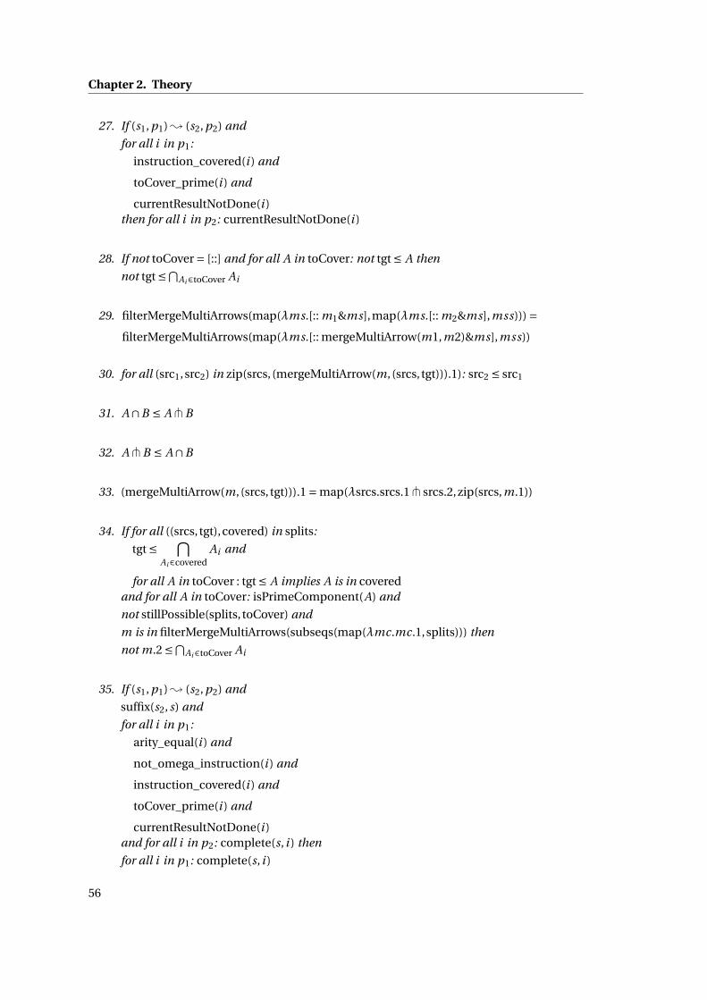
Chapter 2. Theory
27. If (s1, p1)↝ (s2, p2) and
for all i in p1:
instruction_covered(i ) and
toCover_prime(i ) and
currentResultNotDone(i )then for all i in p2: currentResultNotDone(i )
28. If not toCover = [::] and for all A in toCover: not tgt ≤ A then
not tgt ≤⋂Ai∈toCover Ai
29. filterMergeMultiArrows(map(λms.[:: m1&ms],map(λms.[:: m2&ms],mss))) =filterMergeMultiArrows(map(λms.[:: mergeMultiArrow(m1,m2)&ms],mss))
30. for all (src1, src2) in zip(srcs, (mergeMultiArrow(m, (srcs, tgt))).1): src2 ≤ src1
31. A∩B ≤ A ⋔B
32. A ⋔B ≤ A∩B
33. (mergeMultiArrow(m, (srcs, tgt))).1 = map(λsrcs.srcs.1⋔ srcs.2,zip(srcs,m.1))
34. If for all ((srcs, tgt),covered) in splits:
tgt ≤ ⋂Ai∈covered
Ai and
for all A in toCover : tgt ≤ A implies A is in coveredand for all A in toCover: isPrimeComponent(A) and
not stillPossible(splits, toCover) and
m is in filterMergeMultiArrows(subseqs(map(λmc.mc.1,splits))) then
not m.2 ≤⋂Ai∈toCover Ai
35. If (s1, p1)↝ (s2, p2) and
suffix(s2, s) and
for all i in p1:
arity_equal(i ) and
not_omega_instruction(i ) and
instruction_covered(i ) and
toCover_prime(i ) and
currentResultNotDone(i )and for all i in p2: complete(s, i ) then
for all i in p1: complete(s, i )
56

2.5. Verified Enumerative Type Inhabitation in FCL
36. If (s1, p1)↝∗ (s2, [::]) and
for all i in p1:
arity_equal(i ) and
not_omega_instruction(i ) and
instruction_covered(i ) and
toCover_prime(i ) and
currentResultNotDone(i )then for all i in p1: complete(s2, i )
PROOF Statement 36 is the interesting property to show. The complete-predicate is applied
to all the initial instructions and the final state. For each instruction it ensures that the state
includes a multi arrow sufficient to represent all possible merged solution subsets of multi
arrows specified in the instruction, including the current result if present. Merged multi arrow
subsets are only possible solutions if their merged target meets the goal, i.e., it has to be a
subtype of all the types to cover by the instruction. A multi arrow is sufficient to represent a
merged subset multi arrow, if its sources are greater or equal and the target is enough to meet
the goal. For example multi arrow ([::a],b) is sufficient to represent ([::a ∩ c],b ∩d) if only b
is to cover: sources of resulting multi arrows will eventually become recursive inhabitation
targets and the terms inhabiting a include all the terms inhabiting a ∩b. Just like the proof
for soundness, the proof for statement 36 requires induction, decomposition of the first step
and then reasoning backwards. Statements 5, 6, 7, 17, and 27 make it possible to apply the
induction hypothesis by showing that invariants still hold after the first step. Each of them is
proven by case-analysis on the derivation. Backwards reasoning is provided by statement 35.
It requires a detailed and careful case analysis on the many possibilities to derive (s1, p1)↝
(s2, p2).
During this analysis all the invariants have to be taken into account. Invariant arity_equal
ensures, that all multi arrows in an instruction have the same number of sources: type (a →b → c)∩ (d → e) can be used to inhabit c and (b → c)∩e but not c ∩e which would require the
multi arrows ([:: b&[::a]],c) and ([::d ],e) with different numbers of sources. Late termination
is prevented by not_omega_instruction and currentResultNotDone. Late termination would
occur if the target of the current result in an instruction is smaller or equal than all of the types
to cover (invariant currentResultNotDone). Alternatively, if there is no current target, there
could be no types to cover. Both situations would lead to unnecessarily specialized sources,
restricting recursive inhabitation targets to types too small. Invariant not_omega_instruction
asserts that normal operation of the machine will stop before the targets to cover by an
instruction are empty. Also targets greater than ω have to be sorted out before starting the
machine. This is because subtype rule (→ω) converts any such target to an arrow of arbitrary
length, which is incompatible with invariant arity_equal. Machine operations also rely on the
possibility to discharge targets in toCover by adding multi arrows one-by-one. This is possible
if the targets are prime (asserted by invariant toCover_prime): for a prime target tgt and multi
arrows m1 and m2, m1.2∩m2.2 ≤ tgt if m1.2 ≤ tgt or m2.2 ≤ tgt and no distribution across m1
57

Chapter 2. Theory
and m2 has to be taken into account. When processing a single multi arrow, its covered targets
are classified by partitionCover according to their relevance for the remaining targets to cover.
In splits each multi arrow is paired with its covered targets, allowing partitionCover to test for
equality instead of performing costly subtype checks. Invariant instruction_covered ensures
multi arrows are exactly paired with targets they cover. Inclusion of too few targets would
render CHECK and SKIP-steps incomplete by triggering premature exclusion of possibilities.
For the other steps, too many covered targets for a single multi arrow exclude future choices
by removing too many elements from the targets yet to cover.
The rest of the statements of Lemma 24 are technical necessities that simplify backward
reasoning in statement 35 and maintaining the invariants across steps. None of them are
particularly difficult if they are proven in the order presented. ■
There is another important soundness property, which will be proven next.
Lemma 25 (Target Soundness) Target soundness is defined as a Boolean predicate on states
s ∈ (T∗×T)∗ and programs p ∈ I∗Cover:
tgt_sound(s, p) =for all (srcs, tgt) in s :
there exists i i n p s.t. tgt ≤ ⋂Ai∈∆
Ai
for ∆=
⎧⎪⎪⎪⎪⎪⎪⎪⎪⎪⎪⎨⎪⎪⎪⎪⎪⎪⎪⎪⎪⎪⎩
[:: currentResult.2&toCover]
for i = ContinueCover splits toCover currentResult or
i = CheckContinueCover splits toCover currentResult
toCover
for i = Cover splits toCover or
i = CheckCover splits toCover
For i ∈ ICover, and p1, p2 ∈ I∗Cover, and s1, s2 ∈OCover the following statements are true:
1. If (s1, p1)↝ (s2, p2) and for all i in p1: instruction_covered(i ) then
tgt_sound(take(lsize(s2)− lsize(s1), s2), p1)
2. If (s1, [::i ])↝ (s2, p2) and instruction_covered(i ) and tgt_sound(s, p) then
tgt_sound(s, [::i ])
3. If (s1, p1)↝∗ (s2, p2) and for all i in p1: instruction_covered(i ) then
tgt_sound(take(lsize(s2)− lsize(s1), s2), p1)
PROOF Target soundness ensures that the target of every multi arrow in the result state s
covers at least one of the sets specified in an instruction (and the associated intermediate
result if it exists). The proof is similar to the proofs of Lemma 24.36 and Lemma 23.5. It again
58

2.5. Verified Enumerative Type Inhabitation in FCL
combines forwards and backwards reasoning after an induction on the machine steps and de-
composition of state and programs using the machine stack behavior established in Lemma 22.
Forward and backward steps are proven by case analysis on the derivation, where the back-
wards reasoning in statement 2 has been further simplified to account for just one instruction
(decomposition with Lemma 22 is strong enough for this). Invariant instruction_covered again
prevents the final state from becoming too small because of premature result exclusion. ■
The five preconditions for completeness in Lemma 24.36 make proper initialization mandatory.
Additionally types in context Γ have to be preprocessed into multi arrows to be accepted in
instructions. This preprocessing is performed by function splitTy defined next.
Definition 26 (Preprocessing Types into Multi Arrows) The list of lists of all multi arrows of
equal length for a given type A is computed by splitTy :T→ ((T∗×T)∗)∗
splitTy(A) =⎧⎨⎩[::] for isOmega(A)
[:: ([::], A)&splitRec(A, [::], [::])] otherwise
splitRec(A, srcs,∆) =
⎧⎪⎪⎪⎪⎪⎪⎪⎪⎪⎪⎪⎪⎪⎪⎪⎪⎪⎨⎪⎪⎪⎪⎪⎪⎪⎪⎪⎪⎪⎪⎪⎪⎪⎪⎪⎩
[:: [:: ([:: A1&srcs], A2)&∆1]&splitRec(A2, [:: A1&srcs],∆2)]
for A = A1 → A2 and (∆1,∆2) = safeSplit(∆)
splitRec(A2, srcs,∆) for A = A1 ∩ A2 and isOmega(A1)
splitRec(A1, srcs,∆)
for A = A1 ∩ A2 and isOmega(A2) and not isOmega(A2)
splitRec(A1, srcs,splitRec(A2, srcs,∆))
for A = A1 ∩ A2 and not isOmega(A2) and not isOmega(A2)
∆ otherwise
safeSplit(∆) =
⎧⎪⎪⎪⎨⎪⎪⎪⎩([::], [::]) for ∆= [::]
(∆′, [::]) for ∆= [::∆′]
(∆1,∆2) for ∆= [::∆1&∆2]
□
Function splitTy first sorts out types equal to ω and then proceeds recursively on the type
structure. During recursion the sources of the multi arrow currently under construction and a
list ∆ of computed results are maintained. For constructor symbols and products recursion
stops, returning the computed results. These already include the current type as target from
a previous step. Intersections are processed component-wise, again filtering out all types
equal to ω. For arrows the result list is split into a head and tail list. The head list contains all
results with lsize(srcs)+1 sources and a new multi arrow constructed from the current arrow is
59

Chapter 2. Theory
inserted into it. The remaining arrows of the current arrow target are recursively constructed
from the tail list, which contains the results with more sources. The current source is added to
the sources for arrows under construction.
Lemma 26 (Properties of Type Preprocessing) Define the recursive Boolean predicate
arity_increasing(n,∆) =⎧⎪⎪⎨⎪⎪⎩true for ∆= [::]
arity_increasing(n +1,∆2) and
for all (srcs, tgt) in ∆1 : n = lsize(srcs)
for ∆= [::∆1&∆2]
For c ∈ C, n ∈N, and srcs,srcs1, srcs2 ∈T∗, and A,B ∈ T y pes, and ∆,∆1,∆2,∆3 ∈ ((T∗×T)∗)∗,
and f : (T∗×T)∗ → (T∗×T)∗ the following statements are true:
1. arity_increasing(n,∆1 ++∆2) iff
arity_increasing(n,∆1) and arity_increasing(n + lsize(∆1),∆2)
2. If arity_increasing(lsize(srcs)+1,∆) then
arity_increasing(lsize(srcs)+1,splitRec(A, srcs,∆))
3. arity_increasing(0,splitTy(A))
4. For all ms in ∆: for all (srcs1, tgt1) in ms: for all (srcs2, tgt2) in ms:
lsize(srcs1) = lsize(srcs2)
5.⋂
mi∈nth([::],splitRec(A,srcs,∆),n) mkArrow(mi ) ≤⋂mi∈nth([::],∆,n) mkArrow(mi )
6. If lsize(∆1) = lsize(∆2) then lsize(splitRec(A, srcs,∆1)) = lsize(splitRec(A, srcs,∆2))
7. If lsize(∆1) = lsize(∆2) and⋂mi∈nth([::],∆1,n) mkArrow(mi ) ≤⋂
mi∈nth([::],∆2,n) mkArrow(mi ) then⋂mi∈nth([::],splitRec(A,srcs,∆1),n) mkArrow(mi ) ≤⋂
mi∈nth([::],splitRec(A,srcs,∆2),n) mkArrow(mi )
8. If B ≤⋂mi∈nth([::],splitRec(A,srcs,nseq(lsize(∆),[::])),n) mkArrow(mi ) and
B ≤⋂mi∈nth([::],∆,n) mkArrow(mi ) then
B ≤⋂mi∈nth([::],splitRec(A,srcs,∆),n) mkArrow(mi )
9. If mkArrow(srcs, A) ≤⋂mi∈nth([::],∆,n) mkArrow(mi ) then
mkArrow(srcs, A) ≤⋂mi∈nth([::],splitRec(A,srcs,∆),n) mkArrow(mi )
10. A ≤⋂mi∈nth([::],splitTy(A),n) mkArrow(mi )
60

2.5. Verified Enumerative Type Inhabitation in FCL
Define
• merge(∆1,∆2) =⎧⎪⎪⎪⎨⎪⎪⎪⎩[:: ms1 ++ms2&merge(∆′
1,∆′2)] for ∆1 = [:: ms1&∆′
1] and ∆2 = [:: ms2&∆′2]
∆2 for ∆1 = [::]
∆1 for ∆2 = [::]
• splitTy_slow(A) =⎧⎪⎪⎪⎪⎪⎪⎪⎪⎪⎪⎪⎨⎪⎪⎪⎪⎪⎪⎪⎪⎪⎪⎪⎩
[::] for isOmega(A)
[:: [::([::], A1 → A2)]&map(λms.map(λm.(rcons(m.1, A1),m.2),ms),splitTy_slow(A2)]
for A = A1 → A2 and not isOmega(A)
[:: [::([::], A1 ∩ A2)]&behead(merge(splitTy_slow(A1),splitTy_slow(A2)))]
for A = A1 ∩ A2 and not isOmega(A)
[::[::([::], A)]] for not isOmega(A)
then:
11. merge(merge(∆1,∆2),∆3) = merge(∆1,merge(∆2,∆3))
12. merge(∆, [::]) =∆
13. merge([::],∆) =∆
14. splitRec(A, srcs,∆) = merge(splitRec(A, srcs, [::]),∆)
15. If for all ms1,ms2 ∈ (T∗×T)∗: f (ms1 ++ms2) = f (ms1)++ f (ms2) then
map( f ,merge(∆1,∆2)) = merge(map( f ,∆1),map( f ,∆2))
16. splitRec(A, srcs1 ++srcs2, [::]) =map(λms.map(λm.(m.1++srcs2,m.2),ms),splitRec(A, srcs1, [::]))
17. splitTy(A) = splitTy_slow(A)
18. If isOmega(A) then splitTy_slow(A) = [::]
19. nth([::],merge(mss1,mss2),n) = nth([::],mss1,n)++nth([::],mss2,n)
20. nth([::],splitTy_slow(A2),n +1) ⊑ nth([::],splitTy_slow(A1 ∩ A2),n +1)
21. If c(A) ≤ mkArrow(srcs,B) then
(mergeMultiArrows(
filter(
λm. lsize(m.1) = lsize(srcs) and for all (src1, src2) in zip(srcs,m.1) : src1 ≤ src2,
nth([::],splitTy(c(A)), lsize(srcs))))).2 ≤ B
61

Chapter 2. Theory
22. If A1⋆ A2 ≤ mkArrow(srcs,B) then
(mergeMultiArrows(
filter(
λm. lsize(m.1) = lsize(srcs) and for all (src1, src2) in zip(srcs,m.1) : src1 ≤ src2,
nth([::],splitTy(A1⋆ A2), lsize(srcs))))).2 ≤ B
23. If ω≤ mkArrow(srcs,B) then
(mergeMultiArrows(
filter(
λm. lsize(m.1) = lsize(srcs) and for all (src1, src2) in zip(srcs,m.1) : src1 ≤ src2,
nth([::],splitTy(ω), lsize(srcs))))).2 ≤ B
24. If A ≤ mkArrow(srcs,B) then
(mergeMultiArrows(
filter(
λm. lsize(m.1) = lsize(srcs) and for all (src1, src2) in zip(srcs,m.1) : src1 ≤ src2,
nth([::],splitTy(A), lsize(srcs))))).2 ≤ B
25. If A ≤ mkArrow(srcs,B) and not isOmega(mkArrow(srcs,B)) then
exists m in filterMergeMultiArrows(subseqs(nth([::],splitTy(A), lsize(srcs)))), s.t.
lsize(m.1) = lsize(srcs) and
for all (src1, src2) in zip(srcs,m.1) : src1 ≤ src2 and
m.2 ≤ B
PROOF Statements 1-10 prove soundness of splitTy with respect to its specification. The
resulting multi arrows are ordered increasing by their source count (statement 3). After re-
combination with mkArrow, type A is less than each of the multi arrows it includes (statement
10). When done in the order presented, proofs are unsurprising and follow by induction on
the first context mentioned in statement 1 and 2, and structural induction on the type that is
split in the other statements. Completeness is specified in statement 25 and requires a less
straight-forward proof. The main difficulty is to find invariants for the accumulated result
state ∆ in the definition of splitRec. Instead the proof strategy is to replace splitTy by a slower
version splitTy_slow with linear overhead for list concatenation instead of constant overhead
for manipulating the head of the lists. Some easy proofs show that this slower version produces
equal results (statements leading up to 17) and behaves well with ω, distribution of multi
arrows, and intersections (statements 18 - 20). Finally, the completeness proof in statement
25 follows from its alternative representation in 24, which constructs the desired multi arrow
selection to provide completeness instead of postulating its existence. The proof of statement
24 proceeds by structural induction on A. The easier cases for constructors, products and
omega are managed by 21, 22, and 23. The case for ω, 23, is immediate, while for the other
cases reverse induction on the list of sources has to be performed. Then splitTy is replaced by
splitTy_slow, which can be evaluated one step before replacing it again with splitTy to be able
62
2.5. Verified Enumerative Type Inhabitation in FCL
to use induction hypotheses which are otherwise not applicable to the evaluated recursive
calls to splitTyRec. ■
Preprocessing types allows for proper calls to the cover machine.
Lemma 27 (Proper Cover Machine Calls) For ms ∈ (T∗ ×T)∗, srcs ∈ T∗, and A,B ∈ T, and
s ∈OCover, with B s = primeFactors(B), and mss = splitTy(A) the following statements are true:
1. for all i in map(λms.map(λm.(m,filter(λB.m.2 ≤ B ,B s)),ms),mss):
instruction_covered(i )
2. If A ≤ mkArrow(srcs,B) and not isOmega(B) and
([::],map(λms.Cover (map(λm.(m,filter(λB.m.2 ≤ B ,B s)),ms)) B s,mss))↝∗ (s, [::]) then
there exists m in s, s.t.
lsize(m.1) = lsize(srcs) and
for all (src1, src2) in zip(srcs,m.1) : src1 ≤ src2 and
m.2 ≤ B
3. If for all m1 in ms: for all m2 in ms: lsize(m1) = lsize(m2) then⋂mi∈ms mkArrow(mi ) ≤ mkArrow(mergeMultiArrows(ms))
4. If not isOmega(B) and
([::],map(λms.Cover (map(λm.(m,filter(λB.m.2 ≤ B ,B s)),ms)) B s,mss))↝∗ (s, [::]) then
for all m in s: A ≤ mkArrow(m)
5. If ([::],map(λms.Cover (map(λm.(m,filter(λB.m.2 ≤ B ,B s)),ms)) B s,mss))↝∗ (s, [::])
then for all m in s: m.2 ≤ B
PROOF Statement 1 establishes the instructionsCovered invariant later used for Lemma 24.36
in statement 2 and Lemma 25.3 in statement 5. It easily follows from the definitions of map
and filter. Statement 2 proves completeness: for any multi arrow (srcs,B) greater or equal
than A, a subtype compatible multi arrow with the same number of sources can be found
in the final state of the cover machine. The proof uses Lemma 24.36. Its preconditions
are provided using Lemma 26.3 with Lemma 26.4, Lemma 9.17, statement 1, Theorem 2.3,
and observing that no intermediate results are present in the initial input. Statement 3 is
proven by induction on ms. The soundness proof in statement 4 proceeds by instantiating
Lemma 23.9 and Lemma 26.10, induction on s, and combining the instantiated lemmas with
subtype transitivity and statement 3. Finally, target soundness in statement 5 follows from
Theorem 2.1, Lemma 25.3 with statement 5, and transitivity of subtyping. ■
A final post processing step is applied to the results of the cover machine. Sometimes indepen-
dent choices can lead to redundancy, e.g. in (a∩b → c∩d)∩(a → c)∩(b → d) with target c∩d
the machine has to independently inspect possibilities for (a → c)∩ (b → d) for an execution
branch not choosing a ∩b → c ∩d . This leads to duplicated inclusion of a ∩b → c ∩d in the
results. Fortunately, these duplicates can easily be removed.
63

Chapter 2. Theory
Definition 27 (Cover Machine Result Reduction) The result reduction function defined re-
cursively on its input list:
reduceMultiArrows : (T∗×T)∗ → (T∗×T)∗
reduceMultiArrows(ms) =⎧⎪⎪⎪⎪⎪⎪⎪⎪⎪⎪⎪⎪⎪⎪⎪⎪⎪⎪⎪⎪⎪⎪⎪⎪⎪⎪⎪⎪⎪⎪⎪⎪⎪⎪⎪⎨⎪⎪⎪⎪⎪⎪⎪⎪⎪⎪⎪⎪⎪⎪⎪⎪⎪⎪⎪⎪⎪⎪⎪⎪⎪⎪⎪⎪⎪⎪⎪⎪⎪⎪⎪⎩
msr
for ms = [:: m1&ms′] and
msr = reduceMultiArrows(ms′) and
exists (srcs, tgt) in msr s.t.
lsize(srcs) = lsize(m1.1) and
for all (src1, src2) in zip(m1.1,srcs) : src1 ≤ src2
[:: m1&ms′r ]
for ms = [:: m1&ms′] and
msr = reduceMultiArrows(ms′) and
not exists (srcs, tgt) in msr s.t.
lsize(srcs) = lsize(m1.1) and
for all (src1, src2) in zip(m1.1,srcs) : src1 ≤ src2
and ms′r = filter(λm2.not ( lsize(m2.1) = lsize(m1.1) and
for all (src1, src2) in zip(m2.1,m1.1) :
src1 ≤ src2),msr )
[::] otherwise
Lemma 28 (Cover Machine Result Reduction Properties) For ms ∈ (T∗×T)∗, srcs ∈T∗, and
A,B , tgt ∈T function reduceMultiArrows has the following properties:
1. reduceMultiArrows(ms) ⊑ ms
2. If for all m in ms: A ≤ mkArrow(m) then
for all m in reduceMultiArrows(ms): A ≤ mkArrow(m)
3. If for all m in ms: m.2 ≤ B then
for all m in reduceMultiArrows(ms): m.2 ≤ B
4. If for all m in ms: m.2 ≤ B and
exists m in ms, s.t.
lsize(m.1) = lsize(srcs) and
for all (src1, src2) in zip(srcs,m.1) : src1 ≤ src2 and
m.2 ≤ Bthen exists m in reduceMultiArrows(ms), s.t.
lsize(m.1) = lsize(srcs) and
for all (src1, src2) in zip(srcs,m.1) : src1 ≤ src2 and
m.2 ≤ B
64
2.5. Verified Enumerative Type Inhabitation in FCL
PROOF Statement 1 is shown by induction on ms and the (target) soundness preservation
properties of statements 2 and 3 immediately follow from it. Completeness preservation,
which is stated in 4, is proven by induction on ms and case analysis on the conditions checked
by reduceMultiArrows. ■
2.5.2 Generation of Tree Grammars
Results of the cover machine are combined into tree grammars, which allow for easy enumer-
ation. This section discusses an algorithm, which grows these tree grammars in a step-wise
way. Its correctness properties are specified and proven. Specifically the set of inhabitants of a
requested type coincides with the language of the resulting grammar.
Definition 28 (Regular Normalized Tree Grammar and their Language) In [42], chapter 2,
regular normalized tree grammars are defined by G = (S, N ,F ,R), where
• S ∈ N is an axiom (start symbol)
• N is a set of non terminal symbols
• F is a set of terminal symbols disjoint from N
• R is a set of rules of shape A ↦→ f (A1, A2, . . . , An) or A ↦→ f
where f ∈F , and A, A1, A2, . . . An ∈ N
• Arities are used consistently, i.e. if f ∈F occurs in r1,r2 ∈ R then either there exists some
n ∈N and for i ∈ 1,2 and 1 ≤ k ≤ n: Ai , Aik ∈ N s.t. either r1 = A1 ↦→ f (A1
1, A12, . . . , A1
n) and
r2 = A2 ↦→ f (A21, A2
2, . . . , A2n) or there exist A1, A2 ∈ N s.t. r1 = A1 ↦→ f and r2 = A2 ↦→ f .
Language L(G , A) for start symbol A is the least set closed under the following rules:
A ↦→ f ∈ R
f ∈ L(G , A)
A ↦→ f (A1, A2, . . . , An) ∈ R tk ∈ L(G , Ak ) for k ∈ {1,2, . . . ,n}
f (t1, t2, . . . , tn) ∈ L(G , A)
Additionally language L(G) is defined to be L(G ,S). □
Tree Grammars are well-studied concepts with good formal properties. These include efficient
decision procedures for emptiness, uniqueness, and infinity of their associated languages,
as well as an equivalent machine model, non-deterministic finite tree-automata (NFTA) [42].
Note that the associated NFTA model can express the same languages but is algorithmically
weaker than the alternating tree-automata constructed in [165]: transforming a given alter-
nating automaton into an automaton without alternation introduces exponential blowup.
65

Chapter 2. Theory
Rehof and Urzyczyn [165] state that this blowup occurring in addition to the already expo-
nential worst-case size prevents the alternating automaton construction from being a good
solution for deciding inhabitation with subtyping. The tree grammar approach does not intro-
duce double exponential blowup: for input size n there exist polynomial functions p1, p2, p3
such that there can be up to 2p1(n) calls to the cover machine, which by Lemma 21.2 takes
at most 2p2(n) steps, adding at most p3(n) many recursive targets (multi arrow sources) per
step. The resulting tree grammar only contains rules for those targets, so its size is bound
by 2p1(n) ·2p2(n) ·p3(n) ≤ 2p1(n)+p2(n)+log(p3(n)). Intuitively, the reason for the performance im-
provement compared to the alternating automaton approach is that alternation elimination is
oblivious of the fact that the task of the cover machine is independent from the main algorithm
loop. It computes the powerset of main loop and cover computation states, instead of their
Cartesian product.
The main algorithm and its helper functions are defined next. The behavior is specified as a
machine performing step-wise transformations of rule lists for tree grammars.
Definition 29 (Inhabitation Machine) For Γ : B →T define:
• The preprocessed multi arrow context Γ′ : B → ((T∗×T)∗)∗
Γ′(c) = splitTy(Γ(c))
• The set of all possible rules
R ∋ r ::= A ↦→⊥ | A ↦→ c | A ↦→ @(B ,C )
for c ∈ B, and A,B ,C ∈T
• Function computeFailExisting :R∗×T→B×B
computeFailExisting(G , A) =⎧⎪⎪⎪⎪⎪⎪⎪⎪⎪⎪⎪⎪⎪⎪⎨⎪⎪⎪⎪⎪⎪⎪⎪⎪⎪⎪⎪⎪⎪⎩
(true,true) for G = [:: A ↦→⊥&G ′]
(true, exists A ↦→⊥ in G ′) for G = [:: B ↦→⊥&G ′] and not A = B and A ≤ B
computeFailExisting(G ′, A) for G = [:: B ↦→⊥&G ′] and not A = B and not A ≤ B
computeFailExisting(G ′, A) for G = [:: B ↦→ c&G ′]
(false, true) for G = [:: B ↦→ @(C , A)&G ′]
computeFailExisting(G ′, A) for G = [:: B ↦→ @(C ,D)&G ′] and not A = D
(false, false) otherwise
66

2.5. Verified Enumerative Type Inhabitation in FCL
• Function commitMultiArrow :R∗×B× (T∗×T) →R∗
commitMultiArrow(G ,c, (srcs, tgt)) =⎧⎪⎪⎪⎨⎪⎪⎪⎩commitMultiArrow([:: tgt ↦→ @(src → tgt,src)&G],c, (srcs′, src → tgt))
for srcs = [:: src&srcs′]
[:: tgt ↦→ c&G] otherwise
• Function commitUpdates :R∗×T×B× (T∗×T)∗ →R∗
commitUpdates(G , tgt,c,covers) =⎧⎪⎪⎪⎨⎪⎪⎪⎩commitUpdates(commitMultiArrow(G ,c, srcs, (srcs, tgt)), tgt,c,covers′)
for covers = [:: (srcs, tgt′)&covers′]
G otherwise
• Function dropTargets :R∗ →R∗
dropTargets(G) =⎧⎨⎩dropTargets(G ′) for G = [:: A ↦→ @(B ,C )&G ′] or G = [:: A ↦→⊥&G ′]
G otherwise
• Function accumulateCovers : (B → (T∗×T)∗)×T×T∗× (R∗×B)×B →R∗×B
accumulateCovers(Γ′, tgt, toCover,(G , failed),c) =(commitUpdates(G , tgt,c, reduceMultiArrows(covers)), failed and covers = [::])
for p = map(λms.Cover (map(λm.(m,filter(λB.m.2 ≤ B , toCover)),ms)) toCover,
Γ′(c)) and
([::], p)↝∗ (covers, [::])
• Function inhabit_cover : (B → (T∗×T)∗)×R∗×T→B×R∗
inhabit_cover(Γ′,G , tgt) =⎧⎪⎪⎪⎪⎪⎪⎪⎨⎪⎪⎪⎪⎪⎪⎪⎩
(false,G ++ G′)
for (false,G ′) = foldl(λs c.accumulateCovers(Γ′, tgt,primeFactors(tgt), s,c),
([::], true),
enum(B))
(true,G) otherwise
67

Chapter 2. Theory
• Function Gω :T→R∗
Gω(A) = [:: A ↦→ @(A, A)&map(λc.A ↦→ c,enum(B))]
• The machine state transition function
inhabitation_step : (B → (T∗×T)∗)×R∗×R∗ →R∗×R∗
inhabitation_step(Γ′,Gstable,Gtargets) =⎧⎪⎪⎪⎪⎪⎪⎪⎪⎪⎪⎪⎪⎪⎪⎪⎪⎪⎪⎪⎪⎪⎪⎪⎪⎪⎪⎪⎪⎪⎪⎪⎪⎪⎪⎪⎪⎪⎪⎪⎪⎪⎪⎪⎪⎪⎪⎪⎪⎪⎪⎪⎪⎪⎪⎪⎪⎪⎪⎪⎪⎪⎪⎪⎪⎪⎪⎪⎪⎪⎪⎪⎪⎪⎪⎨⎪⎪⎪⎪⎪⎪⎪⎪⎪⎪⎪⎪⎪⎪⎪⎪⎪⎪⎪⎪⎪⎪⎪⎪⎪⎪⎪⎪⎪⎪⎪⎪⎪⎪⎪⎪⎪⎪⎪⎪⎪⎪⎪⎪⎪⎪⎪⎪⎪⎪⎪⎪⎪⎪⎪⎪⎪⎪⎪⎪⎪⎪⎪⎪⎪⎪⎪⎪⎪⎪⎪⎪⎪⎪⎩
1⃝
⎧⎪⎪⎪⎪⎪⎪⎨⎪⎪⎪⎪⎪⎪⎩
(Gstable,G ′targets)
for A ↦→ c in Gstable
([:: A ↦→ c&Gstable],G ′targets)
for not A ↦→ c in Gstable
for Gtargets = [:: A ↦→ c&G ′targets]
2⃝
⎧⎪⎪⎪⎪⎪⎪⎪⎪⎪⎪⎪⎪⎪⎪⎪⎪⎪⎪⎪⎪⎪⎪⎪⎪⎪⎪⎪⎪⎪⎪⎪⎪⎪⎪⎪⎪⎪⎪⎪⎪⎪⎪⎪⎪⎨⎪⎪⎪⎪⎪⎪⎪⎪⎪⎪⎪⎪⎪⎪⎪⎪⎪⎪⎪⎪⎪⎪⎪⎪⎪⎪⎪⎪⎪⎪⎪⎪⎪⎪⎪⎪⎪⎪⎪⎪⎪⎪⎪⎪⎩
(Gstable,G ′targets)
for A ↦→ @(B , tgt) in Gstable
3⃝
⎧⎪⎪⎪⎪⎪⎪⎪⎪⎪⎪⎪⎪⎪⎪⎪⎪⎪⎪⎪⎪⎪⎪⎪⎪⎪⎪⎪⎪⎪⎪⎪⎪⎪⎪⎪⎨⎪⎪⎪⎪⎪⎪⎪⎪⎪⎪⎪⎪⎪⎪⎪⎪⎪⎪⎪⎪⎪⎪⎪⎪⎪⎪⎪⎪⎪⎪⎪⎪⎪⎪⎪⎩
([:: tgt ↦→⊥&Gstable],dropTargets(G ′targets))
for computeFailExisting(Gstable, tgt) = (true, false)
(Gstable,dropTargets(G ′targets))
for computeFailExisting(Gstable, tgt) = (true,true)
([:: A ↦→ @(B , tgt)&Gstable],G ′targets)
for computeFailExisting(Gstable, tgt) = (false, true)
4⃝
⎧⎪⎪⎪⎪⎪⎪⎪⎪⎪⎪⎪⎪⎪⎪⎪⎨⎪⎪⎪⎪⎪⎪⎪⎪⎪⎪⎪⎪⎪⎪⎪⎩
([:: A ↦→ @(B , tgt)&Gω(tgt)++Gstable],G ′targets)
for isOmega(tgt)
5⃝
⎧⎪⎪⎪⎪⎪⎪⎨⎪⎪⎪⎪⎪⎪⎩
([:: tgt ↦→⊥&Gstable],dropTargets(G ′targets))
for inhabit_cover(Γ′,G ′targets, tgt) = (true,G ′′
targets)
([:: A ↦→ @(B , tgt)&Gstable],G ′′targets)
for inhabit_cover(Γ′,G ′targets, tgt) = (false,G ′′
targets)
for not isOmega(tgt)
for computeFailExisting(Gstable, tgt) = (false, false)
for not A ↦→ @(B , tgt) in Gstable
for Gtargets = [:: A ↦→ @(B , tgt)&G ′targets]
6⃝(Gstable,dropTargets(G ′targets))
for Gtargets = [:: A ↦→⊥&G ′targets]
7⃝(Gstable, [::])
for Gtargets = [::]
68

2.5. Verified Enumerative Type Inhabitation in FCL
Within preprocessed context Γ′ the inhabitation machine transforms lists of rules into lists of
rules . Its behavior is specified by the step relation induced by inhabitation_step:
Γ′ ⊢ (Gstable,Gtargets)↝ inhabitation_step(Γ′,Gstable,Gtargets)
The n-step closure of ↝ is the least relation closed under the rules:
Γ′ ⊢ (Gstable,Gtargets)↝0 (Gstable,Gtargets)
1 Γ′ ⊢ (G1stable,G1
targets)↝ (G2stable,G2
targets) 2 Γ′ ⊢ (G2stable,G2
targets)↝n (G3stable,G3
targets)
Γ′ ⊢ (G1stable,G1
targets)↝n+1 (G3stable,G3
targets)
By definition the n-step closure coincides with transtive reflexive closure:
Γ′ ⊢ (Gstable,Gtargets)↝∗ (G ′stable,G ′
targets) iff
there exists n, s.t. Γ′ ⊢ (Gstable,Gtargets)↝n (G ′stable,G ′
targets).
In proof trees t for Γ′ ⊢ (Gstable,Gtargets)↝n+1 (G ′stable,G ′
targets) the first and second premise are
selected using t .1 and t .2. □
The inhabitation machine with all of its helper functions may seem daunting at first, but its
core idea is simple. Each step transforms two rule lists. The first list Gstable represents rules
of the tree grammar under construction. It is stable because it will only grow by addition of
new rules, while its contents will never be deleted or modified. The second list Gtargets is a
queue of rules under consideration for inclusion into the stable list. When there are no more
entries in Gtargets inhabitation stops and Gstable is completed (case 7⃝). Then the resulting
grammar is G = (A,T, {@}⊎B,R) for rules R = {r | r is in Gstable and not exists A s.t. r = A ↦→⊥}
and the request type A from Γ⊢? : A. There are three options for rules r ∈R. Nonterminals are
types T and used without subtyping. Terminals are combinators B or the apply symbol "@".
Rules always use combinators without arguments and the apply symbol with two arguments.
List Gstable can also include rules of form A ↦→ ⊥, which are not considered for the resulting
grammar. They encode the absence of words (inhabitants) for nonterminal (type) A and allow
the algorithm to abort inhabitation early in certain situations. In each step, the machine
makes a decision based on the first rule in Gtargets. The cases grouped under 1⃝ describe
how to add a combinator rule, which is just copied to the stable grammar if it is not yet
present. The target rule queue Gtargets has an additional internal order. If the cover machine
finds multi arrow m = ([:: A2&[::A1]],B) for target B and combinator c, then Gtargets includes
[:: A1 → A2 → B ↦→ c&[:: A2 → B ↦→ @(A1 → A2 → B , A1)&[:: B ↦→ @(A2 → B , A2)&G ′targets]]]
where G ′targets is either empty or starts with a combinator rule of shape C ↦→ d . Whenever the
69

Chapter 2. Theory
machine detects that an intermediate nonterminal (type) such as A2 is unproductive (has
no inhabitants), all of the targets up to the next combinator are discarded using function
dropTargets (case 7⃝ and multiple subcases of 2⃝). In the example, this aborts inhabitation of
B using m and thereby avoids redundant work for A1. If the first rule on the target queue has
shape A ↦→ @(B , tgt) it is an application rule and processed by case 2⃝. Again, rules which have
already been processed are skipped. Otherwise (case 3⃝) computeFailExisting(Gstable, tgt)
analyzes if enough information has been collected about the next target tgt in Gstable to
continue without extra effort. Function computeFailExisting(Gstable, tgt) returns a tuple of
Booleans. The first Boolean indicates if type tgt or a greater or equal type has been marked
as uninhabited. By FCL rule (≤) type tgt cannot have inhabitants in this case, because they
would also be inhabitants of the marked type. The second Boolean is true if tgt has previously
been used in target position or been directly marked as unproductive. In case 3⃝ unproductive
target types are discarded with the rest of the entries from their multi arrows, and they are
marked unproductive in Gstable unless they have been directly marked before. If tgt has been
previously used and not marked, the current rule A ↦→ @(B , tgt) is added to Gstable and no
further targets are generated. Otherwise, in case 4⃝ the machine checks if ω is a subtype of tgt.
Remember that the cover machine from Definition 21 only works correctly with inputs not
greater or equal than ω (Lemma 27.2, Lemma 27.4). Every combinator c can inhabit Γ(c) ≤ωand therefore by rule (≤) also tgt. Additionally, the subtype rules can derive tgt ≤ω≤ω→ω
resulting in inhabitants of tgt being applicable to other inhabitants of type tgt. The rules in
Gω(tgt) express both of these facts, which is why they and the current rule are added to Gstable.
Every applicative term is derivable by Gω(tgt) and no additional targets are required. Finally,
in case 5⃝ the cover machine is invoked to compute additional inhabitation targets. Functions
inhabit_cover and accumulateCovers generate proper cover machine calls (c.f. Lemma 27)
for the split multi arrows of every combinator, which are precomputed in Γ′. Results of the
cover machine are postprocessed (c.f. Definition 27) and converted for future addition to
Gtargets using commitUpdates and commitMultiArrow. Function commitUpdates adds all
cover machine results for one combinator and commitMultiArrow adds a single result multi
arrow in the order described above. Both inhabit_cover, and accumulateCovers also keep
track of a Boolean to indicate if no cover machine call yielded any results for any combinator.
If this is the case, no inhabitants for tgt can be found. The inhabitation machine then marks
tgt as unproductive and again discards entries from the target queue. Otherwise, the current
rule is added to Gstable and the newly computed targets are enqueued. Note that using a stack
instead of a queue would lead to depth first instead of breadth first search.
Correctness of the inhabitation machine requires a fairly complex proof presented next. There
are two main sources of complexity. The first is the requirement to reuse information from
Gstable to avoid loops caused by cyclic grammar entries (e.g. from type A → A). The other
complex part is reasoning about the partially constructed list Gstable, taking into account
potential future inhabitants from Gtargets which can grow or shrink in any step, potentially
even discarding multiple scheduled targets at once. The easiest part, soundness, is proven first.
Again, the relational machine specification enables reasoning about soundness, completeness,
70

2.5. Verified Enumerative Type Inhabitation in FCL
and termination independently. Also, the initial call to the machine can be constructed after
preconditions for its correct execution have been established.
For the following proofs, membership in the language of the grammar computed by the
inhabitation machine is replaced by a Boolean predicate. This avoids the clumsy notation to
distinguish between the grammar and its rules.
Definition 30 (Boolean Predicate deciding Language Membership) Let G ∈R∗ be rules com-
puted by the subtype machine for some requested type B ∈ T. Then for all types A ∈ T,
and terms M ∈ A the Boolean predicate word : R∗ ×T×A → B is by definition the same
as membership in the computed grammar, i.e. word(G , A, M) iff M ∈ L((B ,T, {@} ⊎ B, {r |r is in G and not exists C s.t. r =C →⊥}, A)):
word(G , A, M) =⎧⎪⎪⎪⎪⎪⎨⎪⎪⎪⎪⎪⎩true for M = c and A ↦→ c is in G
true for M = @(M1, M2) and exists A ↦→ @(B ,C ) in G s.t.
word(G ,B , M1) and word(G ,C , M2)
false otherwise
Lemma 29 (Inhabitation Machine Soundness) For context Γ : B →T define the Boolean pred-
icate FCL_sound :R∗ →B by
FCL_sound(G) = for all r in G :⎧⎪⎪⎪⎨⎪⎪⎪⎩A ≤ Γ(c) for r = A ↦→ c
B ≤C → A for r = A ↦→ @(B ,C )
true otherwise
then the following statements are true for all G ,G1,G2,Gstable,Gtargets,G ′stable,G ′
targets ∈R∗, and
A,B ,C , tgt ∈T, srcs ∈T∗, ms ∈ (T∗×T)∗, c ∈ B, M ∈A, and b ∈B:
1. If FCL_sound(G) and word(G , A, M) then Γ⊢ M : A
2. suffix(dropTargets(G),G)
3. If suffix(G1,G2) and word(G1, A, M) then word(G2, A, M)
4. If suffix(G1,G2) and FCL_sound(G2) then FCL_sound(G1)
5. If FCL_sound(G1) and FCL_sound(G2) then FCL_sound(G1 ++G2)
6. If FCL_sound(G) and Γ(c) ≤ mkArrow((srcs, tgt)) and tgt ≤ A then
FCL_sound(commitMultiArrow(G ,c, srcs, A)
71

Chapter 2. Theory
7. If FCL_sound(G) and
for all m in ms :
Γ(c) ≤ mkArrow(m) and
m.2 ≤ A thenFCL_sound(commitUpdates(G , A,c,ms)
Additionally in the preprocessed context Γ′ : B → ((T∗×T)∗)∗ from Definition 29:
8. If FCL_sound(G) and not isOmega(A) then
FCL_sound(accumulateCovers(Γ′, A,primeFactors(A), (G ,b),c).1)
9. If FCL_sound(G) and not isOmega(A) then
FCL_sound(
(foldl(λ s c.accumulateCovers(Γ′, A,primeFactors(A), s,c), (G ,b),enum(B))).1)
10. If FCL_sound(G) and not isOmega(A) then
FCL_sound((inhabit_cover(Γ′,G , A)).2)
11. If isOmega(A) then FCL_sound(Gω(A))
12. If FCL_sound(Gstable) and FCL_sound(Gtargets) then
FCL_sound((inhabitation_step(Γ′,Gstable,Gtargets)).1) and
FCL_sound((inhabitation_step(Γ′,Gstable,Gtargets)).2)
13. If FCL_sound(Gstable) and FCL_sound(Gtargets) and
Γ′ ⊢ (Gstable,Gtargets)↝∗ (G ′stable,G ′
targets) then
FCL_sound((inhabitation_step(Γ′,G ′stable,G ′
targets)).1) and
FCL_sound((inhabitation_step(Γ′,G ′stable,G ′
targets)).2)
PROOF The crucial trick is to define FCL_sound and to prove proposition 1 by induction on
M . This predicate is term-independent and statements 2 - 5, which are easy to prove, enable
compositional reasoning for all the intermediate rule lists created in the other statements.
These cover the different decisions made by inhabitation_step and in the order presented
their proofs follow by unsurprising case-analysis or induction. ■
A total function for the inhabitation machine step relation is constructed next.
Lemma 30 (Functionality of the Inhabitation Machine)
For all preprocessed contexts Γ′ : B → ((T∗ × T)∗)∗ and rule lists G1stable,G1
targets,G2stable,
G2targets,G3
stable,G3targets ∈R∗ the step relation is functional:
If (G1stable,G1
targets)↝ (G2stable,G2
targets) and (G1stable,G1
targets)↝ (G3stable,G3
targets) then
(G2stable,G2
targets) = (G3stable,G3
targets)
PROOF Direct consequence of the definition via inhabitation_step. ■
72

2.5. Verified Enumerative Type Inhabitation in FCL
Definition 31 (Inhabitation Machine Termination Certificate)
For all preprocessed contexts Γ′ : B → ((T∗×T)∗)∗ and input rule lists Gstable,Gtargets ∈ R∗
termination certificate DomΓ′(Gstable,Gtargets) is a proof tree constructed from the rules of
Γ′ ⊢ (Gstable,Gtargets)↝∗ (G ′stable, [::]) for some G ′
stable ∈R∗. □
Just as for the cover machine (c.f. Definition 24) a tail recursive procedure can now be stated
as implementation of the inhabitation machine.
Definition 32 (Procedure implementing the Inhabitation Machine)
inhabitationMachine(Γ′,Gstable,Gtargets) :
DomΓ′(Gstable,Gtargets) → {G ∈R∗ | Γ′ ⊢ (Gstable,Gtargets)↝∗ (G , [::])}
inhabitationMachine(Γ′,Gstable,Gtargets)(d) =⎧⎪⎪⎪⎨⎪⎪⎪⎩G for Gtargets = [::]
inhabitationMachine(Γ′,G ′stable,G ′
targets)(d .2)
for inhabitation_step(Γ′,Gstable,Gtargets) = (G ′stable,G ′
targets)
□
Termination certificates d ∈ DomΓ′(Gstable,Gtargets) always exist because the growth of Gstable
is limited.
Lemma 31 (Totality of the Inhabitation Machine) For context Γ : B →T and the preprocessed
context Γ′ : B → ((T∗×T)∗)∗ define
• A projection to the parameter types of rules by function parameterTypes :R∗ →T∗
parameterTypes(G) = pmap
⎛⎝λr.
⎧⎨⎩Some(C ) for r = A ↦→ @(B ,C )
None otherwise,G
⎞⎠• All types in rules generated for a multi arrow via grammarTypes :T∗×T→T∗
grammarTypes(srcs, tgt) =⎧⎨⎩[:: src&[:: tgt&grammarTypes(srcs′, src → tgt)]] for srcs = [:: src&srcs′]
tgt otherwise
• All possible parameter types for an initial target by maxParameterTypes :T→T∗
maxParameterTypes(A) =[:: A&flatten(map(λc.flatten(map(λms.flatten(map(λm.
grammarTypes(m)++grammarTypes(m.1, A),
filterMergeMultiArrows(subseqs(ms)))),Γ′(c))),enum(B)))]
73

Chapter 2. Theory
Then for all r ∈R, and G ,Gstable,Gtargets ∈R∗, c ∈ B, and A, src, tgt, tgt′ ∈T, and srcs,∆, toCover ∈T∗, ms ∈ (T∗×T)∗, cs ∈ B∗, b ∈B, and n ∈N the following statements are true:
1. If src is in srcs then src is in grammarTypes(srcs, tgt)
2. mkArrow(take(n, srcs), tgt) is in grammarTypes(srcs, tgt)
3. If for all A in undup(parameterTypes(G)): A is in ∆ and
for all A in srcs: A is in ∆ then
for all A in undup(parameterTypes(commitMultiArrow(G ,c, srcs, tgt))): A is in ∆
4. If for all A in undup(parameterTypes(G)): A is in ∆ and
for all A in srcs: A is in ∆ and
for all m in ms: for all src in m.1: src is in ∆ then
for all A in undup(parameterTypes(commitUpdates(G , tgt,c,ms))): A is in ∆
5. If for all A in undup(parameterTypes(G)): A is in maxParameterTypes(tgt) then
for all A in (accumulateCovers(Γ′, tgt,primeFactors(tgt), (G ,b),c)).1:
A is in maxParameterTypes(tgt)
6. tgt is in maxParameterTypes(tgt)
7. If for all A in undup(parameterTypes(G)): A is in maxParameterTypes(tgt) then
for all A in
undup(parameterTypes(
(foldl(λ s c.accumulateCovers(Γ′, tgt′,primeFactors(tgt′), s,c), (G ,b),enum(B))).1)) :A is in maxParameterTypes(tgt)
8. If for all A in undup(parameterTypes(G)): A is in maxParameterTypes(tgt) then
for all A in undup(parameterTypes((inhabitCover(Γ′,G , tgt)).2)):
A is in maxParameterTypes(tgt)
9. For all A in parameterTypes(Gω(tgt)): A = tgt
10. If tgt′ is in maxParameterTypes(tgt) then
for all A in undup(parameterTypes(Gω(tgt′))): A is in maxParameterTypes(tgt)
11. If for all A in undup(parameterTypes(Gtargets)): A is in maxParameterTypes(tgt) and
for all A in undup(parameterTypes(Gstable)): A is in maxParameterTypes(tgt) then
for all A in undup(parameterTypes((inhabitation_step(Γ′,Gstable,Gtargets)).1)) :
A is in maxParameterTypes(tgt)
and for all A in undup(parameterTypes((inhabitation_step(Γ′,Gstable,Gtargets)).2)) :
A is in maxParameterTypes(tgt)
74

2.5. Verified Enumerative Type Inhabitation in FCL
Define the measured lexicographic product inhabit_step_reltgt ⊂ (R∗×R∗)× (R∗×R∗) as the
least relation closed under the rules:
lsize(maxParameterTypes(tgt))+1− lsize(undup(parameterTypes(Gstable))) <lsize(maxParameterTypes(tgt))+1− lsize(undup(parameterTypes(G ′
stable)))
inhabit_step_reltgt((Gstable,Gtargets), (G ′stable,G ′
targets))
undup(parameterTypes(Gstable)) = undup(parameterTypes(G ′stable))
lsize(undup(parameterTypes(Gtargets))) < lsize(undup(parameterTypes(G ′targets)))
inhabit_step_reltgt((Gstable,Gtargets), (G ′stable,G ′
targets))
Also assert that relation R(x, y) is well-founded [154], written WF(R), if all x are accessible,
written Acc(x), where Acc(x) is the least set closed under the rule:
for all y: if R(y, x) then Acc(y)Acc(x)
Continue with the proof of the following statements:
12. WF(inhabit_step_reltgt)
13. If inhabit_step_reltgt((Gstable,Gtargets), (G ′stable,G ′
targets)) and
for all A in undup(parameterTypes(Gstable)): A is in maxParameterTypes(tgt) then
inhabit_step_reltgt(([:: r &Gstable],Gtargets), (G ′stable,G ′
targets))
14. lsize(dropTargets(Gtargets)) ≤ lsize(Gtargets)
15. If ms = [::] then Gtargets = commitUpdates(Gtargets, tgt,c,ms)
16. If ms = [::] then reduceMultiArrows(ms) = [::]
17. If (accumulateCovers(Γ′, tgt, toCover,(G , true),c)).2 then
G = (accumulateCovers(Γ′, tgt, toCover,(G , true),c)).1
18. If (accumulateCovers(Γ′, tgt, toCover,(G ,b),c)).2 then b = true
19. If (foldl(λs c.accumulateCovers(Γ′, tgt, toCover, s,c), (G ,b),cs)).2 then b = true
20. If (foldl(λs c.accumulateCovers(Γ′, tgt, toCover, s,c), (G ,b),cs)).2 then
G = (foldl(λs c.accumulateCovers(Γ′, tgt, toCover, s,c), (G ,b),cs)).1
21. If (inhabit_cover(Γ′,Gtargets, tgt)).1 then (inhabit_cover(Γ′,Gtargets, tgt)).2 =Gtargets
22. If not (computeFailExisting(G , A)).1 and not (computeFailExisting(G , A)).2 then
A is not in parameterTypes(G)
75
Chapter 2. Theory
23. If for all A in undup(parameterTypes(Gstable)): A is in maxParameterTypes(tgt) and
for all A in undup(parameterTypes(Gtargets)): A is in maxParameterTypes(tgt) and
not Gtargets = [::] then
inhabit_step_reltgt(inhabitation_step(Γ′,Gstable,Gtargets), (Gstable,Gtargets))
24. A finite proof tree DomΓ′([::], (inhabit_cover(Γ′, [::], tgt)).2) can always be constructed
PROOF The first part establishes the maximal list of parameter types that will ever occur
in position C in rules of shape A ↦→ @(B ,C ). These will always stem from the filtered and
merged combination of some multi arrows drawn from Γ′, possibly with their targets replaced
by the initial request type. Function grammarTypes allows all sources and targets of these
multi arrows in the generated set. Statements 1–11 establish the properties of the auxiliary
inhabitation machine functions with respect to the maximal parameters. Their proofs are
by straight-forward induction and/or case analysis. Statement 11 is the most important part
and shown by case analysis on the options considered by the inhabitation machine transition
function inhabitation_step.
Well-foundedness from statement 11 is used to construct the proof tree in statement 24. With
the rule for Acc well-foundedness generates the induction principle
If for all x :
if for all y : R(y, x) implies P (y)
then P (x)
then forall x : P (x)
where P is chosen to be DomΓ′ and statement 23 satisfies the precondition R(y, x) for con-
structing the tree via the induction hypothesis. Statement 11 uses that inhabit_step_rel is the
lexicographic product of two well founded relations (less than on natural numbers), which
is again well-founded [154]. Statements 13–22 break down the proof of 11, which is by case-
analysis on the options of inhabitation_step, into easy to show steps. ■
The initial remark about the upper bound on the number of machine steps and thereby
the size of the grammar can also be clarified further at this point. It is easy to show that
the number of multi arrows in Γ′(c) = splitTy(Γ(c)) is bound by size(A) · length(A). Func-
tion subseqs computes exponentially many subsequences. The subsequences are passed to
filterMergeMultiArrows, which invokes mergeMultiArrows for each subsequence. Function
mergeMultiArrows calls mergeMultiArrow linear many times, which then combines multi
arrows in polynomial time of their size using the quadratic subtyping algorithm. Results are
passed to grammarTypes and processed in linear time. Therefore maxParameterTypes(A) is
overall in 2p(size(A)·length(A)) for some polynomial p. Relation inhabit_step_reltgt bounds the
number of possible steps by (lsize(maxParameterTypes(A))+1)2 because Lemma 31.11 places
all parameters in Gstable and Gtargets within maxParameterTypes(A). There is only one call to
the cover machine per step and its arguments are polynomial in the input size, hence the
overall single-exponential running time of the algorithm.
76

2.5. Verified Enumerative Type Inhabitation in FCL
The final part of the correctness proof, completeness, requires two additional invariants.
Lemma 32 (Inhabitation Machine Invariants) For context Γ : B →T, a list of rules G ∈R∗
• is soundly marked for failures, FailSoundΓ(G), if for all A ∈T s.t. there exists A ↦→⊥ in G
there does not exist M ∈A s.t. Γ⊢ M : A
• is a target list without fail rules, noTargetFailures(G), if there does not exist A ∈T s.t. there
exists A ↦→⊥ in G
Additionally for the preprocessed contextΓ′(c) = splitTy(Γ(c)) as well as all G1,G2,Gstable,Gtargets,
G ′targets ∈R∗, c ∈ B, srcs ∈T∗, and A, tgt ∈T the following statements are true:
1. If FailSoundΓ(G1) and FailSoundΓ(G2) then FailSoundΓ(G1 ++G2)
2. If FailSoundΓ(G1 ++G2) then FailSoundΓ(G1) and FailSoundΓ(G2)
3. If FailSoundΓ(G) and (computeFailExisting(G , A)).1 = true then
FailSoundΓ([:: A ↦→⊥&G])
4. If (accumulateCovers(Γ′, tgt,primeFactors(tgt), (G , true),c)).2 = true and
not isOmega(tgt) then
not Γ⊢ c : mkArrow(srcs, tgt)
5. If (inhabit_cover(Γ′,G , tgt)).1 = true and not isOmega(tgt) then
not exists M ∈A s.t. Γ⊢ M : tgt
6. FailSoundΓ(Gω(A))
7. If FailSoundΓ(Gstable) then FailSoundΓ((inhabitation_step(Γ′,Gstable,Gtargets)).1)
8. If noTargetFailures(Gtargets) and suffix(G ′targets,Gtargets) then noTargetFailures(G ′
targets)
9. If noTargetFailures(Gtargets) then noTargetFailures((inhabit_cover(Γ′,Gtargets, tgt)).2)
10. If noTargetFailures(Gtargets) then
noTargetFailures((inhabitation_step(Γ′,Gstable,Gtargets)).2)
PROOF Statements 1 and 2 follow from the definition of FailSound, while 3 is shown by
induction on G and case analysis of the first rule. The proof for statement 4 uses that Γ(c)
is the minimal type of c (Lemma 16), and completeness of the cover machine (Lemma 24)
after unfolding the definition of accumulateCovers (Definition 29). Statement 5 is shown
by inversion of Γ⊢ M : tgt using Lemma 15.2 and induction on the finite combinator set B.
Statement 6 follows from the definition of Gω(A). Statement 7, sound failure marking, follows
by case analysis on the first rule in Gtargets in combination with the previous statements.
Statement 8 follows from the definition of noTargetFailures, statement 9 by unfolding the
definition of inhabit_cover and induction on the finite combinator set B, and then by use of
statement 10 in the case analysis of the first rule of Gtargets and the prior statements. ■
77

Chapter 2. Theory
Lemma 33 (Inhabitation Machine Completeness) For context Γ : B →T define:
• Function updateGroups : (R∗)∗×R→ (R∗)∗ to group a single rule together with the rules
of the multi arrow it was generated from:
updateGroups(groups,r ) =⎧⎪⎪⎪⎨⎪⎪⎪⎩[:: [::A ↦→ c]&groups] for r = A ↦→ c
[:: rcons(g ,r )&groups′] for groups = [:: g &groups′] and not r = A ↦→ c
[::[::r ]] for groups = [::] and not r = A ↦→ c
• Function group :R∗ → (R∗)∗ to group rules by the multi arrow they were generated from:
group(G) = rev(foldl(λ s r.updateGroups(s,r ), [::],G))
• A projection to the target (left hand side) of a rule lhs :R→T
lhs(r ) = A for r = A ↦→⊥ or r = A ↦→ c or A ↦→ @(B ,C )
• A projection to the targets of a list of rules targetTypes :R∗ →T∗
targetTypes(G) = map(lhs,G)
• Potential future derivability of a term as the least relation future_word ⊆R∗×R∗×T×Aclosed under the rules:
A ↦→ c is in Gstable
future_word(Gstable,Gtargets, A,c)
g is in group(Gtargets)
A ↦→ c is in g
for all B in parameterTypes(g ):
exists M s.t. Γ⊢ M : B
future_word(Gstable,Gtargets, A,c)
A ↦→ @(B ,C ) is in Gstable
future_word(Gstable,Gtargets,B , M)
future_word(Gstable,Gtargets,C , N )
future_word(Gstable,Gtargets, A,@(M , N ))
g is in group(Gtargets)
A ↦→ @(B ,C ) is in g
future_word(Gstable,Gtargets,B , M)
Γ⊢ N : C
for all B in parameterTypes(g ):
exists M s.t. Γ⊢ M : B
future_word(Gstable,Gtargets, A,@(M , N ))
78

2.5. Verified Enumerative Type Inhabitation in FCL
• An intermediate machine state (Gstable,Gtargets) ∈ R∗×R∗ to be partially complete for
initial type tgt ∈T, written FCL_complete(tgt,Gstable,Gtargets), if:
for all A ∈T s.t. A = tgt or
A is in parameterTypes(Gstable) or
A is in targetTypes(pmap(λg .ohead(rev(g )),group(Gtargets))) :
for all M ∈A : Γ⊢ M : A implies future_word(Gstable,Gtargets, A, M)
Then for the preprocessed context Γ′(c) = splitTy(Γ(c)) and all G ,Gstable,Gtargets,G ′stable,G ′
targets,
g ,nextTargets ∈ R∗, groups ∈ (R∗)∗, r ∈ R, and A,B ,C ,D, tgt ∈T, srcs ∈T∗, covers,ms ∈ (T∗×T)∗, c ∈ B, cs ∈ B∗, M ∈A, b ∈B, n ∈N the following statements are true:
1. flatten(group(G)) =G
2. updateGroups([::],r ) = [::[::r ]]
3. If for all r in G: not exists A ∈T and c ∈ B s.t. r = A ↦→ c then
foldl(λ s r.updateGroups(s,r ), [:: g &groups],G) = [:: g ++G&groups]
4. foldl(λ s r.updateGroups(s,c),groups,[:: A ↦→ c&G]) =foldl(λ s r.updateGroups(s,c), [::], [:: A ↦→ c&G])++groups
5. If Gtargets =G ++dropTargets(Gtargets) then
for all r in G: not exists A ∈T and c ∈ B s.t. r = A ↦→ c
6. Either dropTargets(G) = [:: A ↦→ c&G ′] for some A ∈T, c ∈ B, and G ′ ∈R∗ or
dropTargets(G) = [::]
7. If Gtargets =G ++dropTargets(Gtargets) then
group([:: r &Gtargets]) = [:: [:: r &G]&group(dropTargets(Gtargets))]
8. If A = tgt or A is in parameterTypes(Gstable) and
FCL_complete(tgt,Gstable, [::]) and Γ⊢ M : A then
word(Gstable, A, M)
9. If future_word(Gstable, [::], A, M) then word(Gstable, A, M)
10. If future_word(Gstable,Gtargets, A, M) and for all r in Gstable: r is in G ′stable then
future_word(G ′stable,Gtargets, A, M)
11. If A ↦→ c is in Gstable and future_word(Gstable, [:: A ↦→ c&Gtargets],B , M) then
future_word(Gstable,Gtargets,B , M)
12. If future_word(Gstable, [:: A ↦→ @(B ,C )&Gtargets],D, M) and
not exists N ∈A s.t. Γ⊢ N : C then
future_word(Gstable,dropTargets(Gtargets),D, M)
79

Chapter 2. Theory
13. If FailSound(Gstable) and
(computeFailExisting(Gstable,C )).1 = true and
FCL_complete(tgt,Gstable, [:: A ↦→ @(B ,C )&Gtargets]) then
FCL_complete(tgt,G ′stable,dropTargets(Gtargets)) where
G ′stable =
⎧⎨⎩Gstable for (computeFailExisting(Gstable,C )).2 = true
[:: C ↦→⊥&Gstable] otherwise
14. If A ↦→ @(B ,C ) is in Gstable and
FCL_complete(tgt,Gstable, [:: A ↦→ @(B ,C )&Gtargets]) and
future_word(Gstable, [:: A ↦→ @(B ,C )&Gtargets],D, M) then
future_word(Gstable,Gtargets,D, M)
15. If computeFailExisting(G , A) = (false, true) then A is in parameterTypes(G)
16. If isOmega(C ) then future_word(Gω(C )++Gstable,Gtargets,C , M)
17. If future_word(Gstable, [:: A ↦→ @(B ,C )&Gtargets],D, M) and
for all N ∈A: Γ⊢ N : C implies future_word([:: A ↦→ @(B ,C )&Gstable],Gtargets,C , N ) then
future_word([:: A ↦→ @(B ,C )&Gstable],Gtargets,D, M)
18. If isOmega(C ) and FCL_complete(tgt,Gstable, [:: A ↦→ @(B ,C )&Gtargets]) then
FCL_complete(tgt, [:: A ↦→ @(B ,C )&Gω(C )++Gstable],Gtargets)
19. (accumulateCovers(Γ′,C ,primeFactors(C ), (G ,b),c)).1 =(accumulateCovers(Γ′,C ,primeFactors(C ), ([::],b),c)).1++G
20. (foldl(λ s c.accumulateCovers(Γ′,C ,primeFactors(C ), s,c), ([::], true),enum(B))).1 =flatten(map(
λ c.(accumulateCovers(Γ′,C ,primeFactors(C ), ([::], true),c)).1,
rev(enum(B))))
21. If
(foldl(λ s c.accumulateCovers(Γ′,C ,primeFactors(C ), s,c), ([::], true),enum(B))).2 = true
then
(foldl(λ s c.accumulateCovers(Γ′,C ,primeFactors(C ), s,c), ([::], true),enum(B))).1 = [::]
22. commitMultiArrow(G ,c, (srcs, A)) = commitMultiArrow([::],c, (srcs, A))++G
23. commitUpdates(G , A,c,covers) =rev(map(λm. rev(commitMultiArrow([::],c, (m.1, A))),covers))++G
24. lsize(commitMultiArrow([::],c, srcs, tgt)) = 1+ lsize(srcs)
80

2.5. Verified Enumerative Type Inhabitation in FCL
25. nth(tgt ↦→ @(mkArrow(take(lsize(srcs)− (n −1),srcs), tgt),nth(tgt,srcs, lsize(srcs)−n)),
commitMultiArrow([::],c, (srcs, tgt)),n) =⎧⎪⎪⎪⎨⎪⎪⎪⎩mkArrow(srcs, tgt) ↦→ c for n = 0
mkArrow(take(lsize(srcs)−n, srcs), tgt) ↦→ otherwise
@(mkArrow(take(lsize(srcs)− (n −1),srcs), tgt),nth(tgt,srcs, lsize(srcs)−n))
26. If GnextTargets = rev(flatten(map(λ m.commitMultiArrow([::],c, (m.1,C )),ms))) then
GnextTargets = A ↦→ d for some A ∈T and d ∈ B or GnextTargets = [::]
27. If GnextTargets =flatten(map(λ c.(accumulateCovers(Γ′,C ,primeFactors(C ), ([::], true),c)).1,cs)) then
GnextTargets = A ↦→ d for some A ∈T and d ∈ B or GnextTargets = [::]
28. group(commitMultiArrow([::],c, srcs, tgt)) = [::commitMultiArrow([::],c, srcs, tgt)]
29. If future_word([::],Gtargets,D, M) and exists N ∈A s.t. Γ⊢ N : C then
future_word([::],Gtargets ++[::A ↦→ @(B ,C )],D, M)
30. parameterTypes(commitMultiArrow([::],c, srcs, tgt)) = rev(srcs)
31. If future_word(Gstable,Gtargets, A, M) and
G ′targets = [:: A ↦→ c&G] or G ′
targets = [::] then
future_word(Gstable,Gtargets ++G ′targets, A, M)
32. If future_word(Gstable,G ′targets, A, M) and
G ′targets = [:: A ↦→ c&G] or G ′
targets = [::] then
future_word(Gstable,Gtargets ++G ′targets, A, M)
33. If Γ⊢ M : C and not isOmega(C ) then
future_word([::],
flatten(map(λ c.(accumulateCovers(Γ′,C ,primeFactors(C ), ([::], true),c)).1,rev(enum(B))))
C , M)
34. If future_word(Gstable, [:: A ↦→ @(B ,C )&Gtargets],D, M) and not isOmega(C ) then
future_word([:: A ↦→ @(B ,C )&Gstable],
Gtargets ++flatten(map(λ c.(accumulateCovers(Γ′,C ,primeFactors(C ), ([::], true),c)).1,rev(enum(B))),
D, M)
35. If B is in targetTypes(pmap(λ g .ohead(rev(g )),group(targets))) then
B is in targetTypes(pmap(λ g .ohead(rev(g )),group([:: r &targets])))
36. If reduceMultiArrows(covers) = [::] then covers = [::]
81

Chapter 2. Theory
37. If (foldl(accumulateCovers(Γ′,C ,primeFactors(C ), ([::], true),enum(B)))).1 = [::] then
(foldl(accumulateCovers(Γ′,C ,primeFactors(C ), ([::], true),enum(B)))).2 = true
38. For all A in targetTypes(pmap(
λ g .ohead(rev(g )),
group(flatten(map(λ c.(accumulateCovers(Γ′,C ,primeFactors(C ), ([::], true),c)).1,
rev(enum(B)))))) :A =C
39. If not isOmega(C ) and FCL_complete(tgt,Gstable, [:: A ↦→ @(B ,C )&Gtargets]) and
(G ′stable,G ′
targets) =⎧⎪⎪⎪⎨⎪⎪⎪⎩([:: A ↦→ @(B ,C )&Gstable],GnextTargets)
for inhabit_cover(Γ′,Gtargets,C ) = (false,GnextTargets)
([:: C ↦→⊥&Gstable],dropTargets(Gtargets)) otherwise
then FCL_complete(tgt,G ′stable,G ′
targets)
40. If FailSoundΓ(Gstable) and noTargetFailures(Gtargets) and
FCL_complete(tgt,Gstable,Gtargets) then
for (G ′stable,G ′
targets) = inhabitation_step(Γ′,Gstable,Gtargets):
FCL_complete(tgt,G ′stable,G ′
targets)
41. If FailSoundΓ(Gstable) and noTargetFailures(Gtargets) and
FCL_complete(tgt,Gstable,Gtargets) and
Γ′ ⊢ (Gstable,Gtargets)↝∗ (G ′stable,G ′
targets) then
FCL_complete(tgt,G ′stable,G ′
targets)
PROOF The most important trick is to define potential future derivability by future_word. It
extends the language definition of Tree Grammars (Definition 29) to consider rules sched-
uled in Gtargets. If at some point of the derivation of an applicative term list Gstable does
not yet include enough rules, the derivation can be suspended. This suspension is only
possible if Gtargets includes a rule that will – in later machine steps – ensure Gstable is suffi-
cient to continue. The rule is identified by regrouping subsequent Gtargets entries accord-
ing to the multi arrow they originated from. Remember that the cover machine uses [::
A1 → A2 → B ↦→ c&[:: A2 → B ↦→ @(A1 → A2 → B , A1)&[:: B ↦→ @(A2 → B , A2)&G ′targets]]]
for multi arrow m = ([:: A2&[::A1]],B), target B , and combinator c with a split type Γ′(c)
including m. Function group isolates multi arrow entries into separate lists, resulting in
[:: [:: A1 → A2 → B ↦→ c&[:: A2 → B ↦→ @(A1 → A2 → B , A1)&[::B ↦→ @(A2 → B , A2)]]]&groups′].If all the types in parameter positions, i.e. A1 and A2, are inhabited, the group will not
be discarded and its rules can be used to resume suspended derivations of A1 → A2 → B ,
A2 → B , and B . Property FCL_complete(tgt,Gstable,Gtargets) characterizes machine states
Gstable and Gtargets which in future derive all terms M s.t. Γ ⊢ M : tgt. For this additionally
all terms with types in parameter positions of Gstable have to be derivable in future, guaran-
teeing that all choices for N will be considered when Γ ⊢ @(c, N ) : tgt for any c. Moreover,
82

2.5. Verified Enumerative Type Inhabitation in FCL
terms for some of the target types in Gtargets need to be future derivable. Suppose Gstable
includes A ↦→ @(B ,C ) and rules with target type C are not yet included in Gstable, then rules
for all multi arrows with type C are required to be scheduled for future consideration in
Gtargets. However, simply requiring that all terms with target types of rules in Gtargets are fu-
ture derivable is too restrictive. Suppose type A1 in the previous example is uninhabited.
Then group [:: A1 → A2 → B ↦→ c&[:: A2 → B ↦→ @(A1 → A2 → B , A1)&[::B ↦→ @(A2 → B , A2)]]]
does not contribute to future derivability and it will be discarded after encountering rule
A2 → B ↦→ @(A1 → A2 → B , A1). Yet, terms N with Γ ⊢ N : A2 → B might exist (e.g. us-
ing a combinator d : A′2 → B with A2 ≤ A′
2) but not be (future) derivable. For them, rules
[:: A′2 → B ↦→ d&[::B ↦→ @(A′
2 → B , A′2)]] would derive N from non-terminal A′
2 → B instead.
In fact, only terms of the last target type of a group have to be derivable. By the definition
of future_word these terms only exist if all of the parameter types in the group are inhabited
and therefore the group will not be discarded. In the definition of FCL_complete, the part
pmap(λg .ohead(rev(g )),group(Gtargets)) projects all non-empty groups exactly to their last
target types.
Keeping the illustration above in mind, statements of the lemma break down its proof into
manageable components, individually proven by case analysis, induction and use of the
previously established propositions. Statements 1–7 make it possible to reason about func-
tion group used in the definitions of future_word and FCL_complete. Statement 9 is evident
from the definitions of word and future_word. It shows that future derivability is a sufficient
condition for derivability in the final machine state where Gtargets is empty. The direct conse-
quence, proposition 8, justifies to prove FCL_complete(tgt,Gstable, [::]) instead of Γ⊢ M : tgt
implies word(Gstable, M , tgt) to obtain completeness. Proposition 10 allows weakening of fu-
ture derivability from Gstable, showing that future_word is closed under subset membership
of stable rule lists. Statement 11 is the first of multiple absorption properties (c.f. 14, 17, 34)
incorporating rules form Gtargets into Gstable. Specifically, with statement 11 combinator rules
can be removed from Gtargets if they are included in Gstable, possibly because of application
of the prior weakening property. This is in correspondence to case 1⃝ of inhabitation_step
in Definition 29. Statements 12 and 13 justify to discard target rule groups because of unin-
habited parameters identified by computeFailExisting. The previously established invariant
FailSound (Lemma 32) is required to ensure completeness is not lost due to conflicting rules in
Gstable. Absorption rule 14 can remove applicative rules from the targets. It has FCL_complete
as precondition to ensure derivations of the removed rule A ↦→ @(B ,C ), which previously
succeeded in suspended state from Gtargets without further derivation for C , do not get stuck
when replaced by derivations from Gstable that do require C . Rule 14 is used for the last two
situations of case 3⃝, Definition 29. In the first situation the rule to move already existed in
Gstable and this fact is checked by computeFailExisting. Statement 15 proves soundness of the
decision made by computeFailExisting. The other situation is grouped together under 4⃝ and
again subdivided into two cases. Statements 16, 17, and their consequence statement 18 dis-
patch the first case of 4⃝ in which ω is a subtype of the parameter type of the next applicative
rule. For the other situation, 5⃝, function inhabit_cover has to be studied in more depth. The
83

Chapter 2. Theory
analysis proceeds with the auxiliary functions. Statements 19 and 20 allow separate reasoning
about the new entries in Gtargets for individual combinators. By proposition 21 the Boolean
that detects if there are no updates to Gtargets is computed soundly. Statements 22–30 help to
reason about adding multi arrows to the target queue. Analogous to statement 10, the target
queue can grow whilst weakening future_word to include at least the same derivable terms,
which is shown in 31 and 32. This is then used to prove the absorption rule 34 in combination
with future derivability of the terms for its parameter type C in statement 33. Propositions
35–38 provide more properties of grouping collected targets. They relate the target type of
freshly collected grouped rules to the requested parameter type (statement 38) and establish
(statement 37) the other part of correctness for the emptyness detection Boolean previously
addressed in statement 21. Results for case 5⃝ in Definition 29 are combined in proposition 39.
The final statements 40, and 41 are the main properties to show. They establish FCL_complete
as an invariant across machine steps. The poof of 40 is by case analysis on all of the branches
of inhabitation_step, dispatching each branch with the facts proven above. The proof of 41 is
by induction on the machine steps using 40, Lemma 32.7, and Lemma 32.10 for progress. ■
The proof of Lemma 33 is, together with that of Lemma 24, the most intricate of this text
and the interested reader is encouraged to interactively step through the Coq formalization
for all of its details (possibly starting in reverse from Lemma 33.40 to see where which part
becomes necessary). Both proofs have revealed subtle mistakes in initial attempts to define the
machines characterized by their lemmas. Spotting these mistakes would have been impossible
or at least improbable without the aid of Coq as a formal verification system. Also tuning the
delicate definitions of future_word and FCL_complete required multiple attempts, and being
able to automatically re-check which parts were affected by the changes was of great value
during development.
Finally the initial call to the inhabitation machine can be constructed and correctness of the
type inhabitation algorithm can be proven.
Theorem 6 (Type Inhabitation Correctness)
For applicative terms A formed over any finite enumerable combinator base B, and intersection
types T formed over any ≤C-preordered countable set C of type constructor symbols define:
inhabit : (B →T)×T→R∗
inhabit(Γ, A) =⎧⎪⎪⎪⎪⎪⎪⎪⎪⎪⎪⎨⎪⎪⎪⎪⎪⎪⎪⎪⎪⎪⎩
Gω(A) for isOmega(A) = true
inhabitationMachine(λc. splitTy(Γ(c)), [::],Gtargets)(d)
for isOmega(A) = false and
inhabit_cover(λc. splitTy(Γ(c)), [::], A) = ( false,Gtargets) and
d constructed by Lemma 31.24
A ↦→⊥ otherwise
84
2.5. Verified Enumerative Type Inhabitation in FCL
with the following properties for all A ∈T and M ∈A:
1. If word(inhabit(Γ, A), A, M) then Γ⊢ M : A
2. If Γ⊢ M : A then word(inhabit(Γ, A), A, M)
PROOF By case distinction following the branches of inhabit and use of the invariants estab-
lished in Lemma 29, Lemma 32, and Lemma 33. ■
85

Chapter 2. Theory
2.6 Algebraic Interpretation of Results
Terms of the tree grammar computed in Theorem 6 are of little use by themselves. This section
discusses a general algebraic framework to interpret them in different target languages.
2.6.1 Subsorted Σ-Algebra Families
Signatures are a common language for interfaces and connect combinatory logic with synthe-
sis target languages. Families of subsorted signatures allow to model interfaces parametric
and subtype polymorphism.
Definition 33 (Subsorted Signature Families) I -indexed ≤S-subsorted signature families Σ
are defined by Σi∈I = (S,O,arityi ,domi , rangei ) where
• I is a set of indexes
• S is a set of sorts ordered by a preorder (reflexive, transitive) relation ≤S⊆S×S
• O is a finite set of operations
• arity : (O→N)i∈I is a family of functions, assigning an arity to each operation
• dom :
((arityi (o)∏
n=1S
)o∈O
)i∈I
is a family of families of vectors, assigning a domain, which is
a vector of arityi (o) sorts, to each operation
• range : ((S)o∈O)i∈I is a family of families of sorts, assigning a range to each operation. □
Restricting I to a singleton set yields traditional subsorted signatures described in [83]. Further,
the restriction ≤S= {(s, s) | s ∈S} results in many-sorted signatures [70; 71; 150]. Less trivial
restrictions on the parameter set I and their implications on the equations that can be imposed
on interpretations have been investigated in [148]. Signatures where S is a singleton have also
been studied [109]. Avoiding any meta-theoretic issues and simplifying the Coq formalization,
from now on all sort sets S are additionally assumed to be countable and ≤S is assumed to
be decidable. The following example illustrates the roles of the different components of a
signature.
86
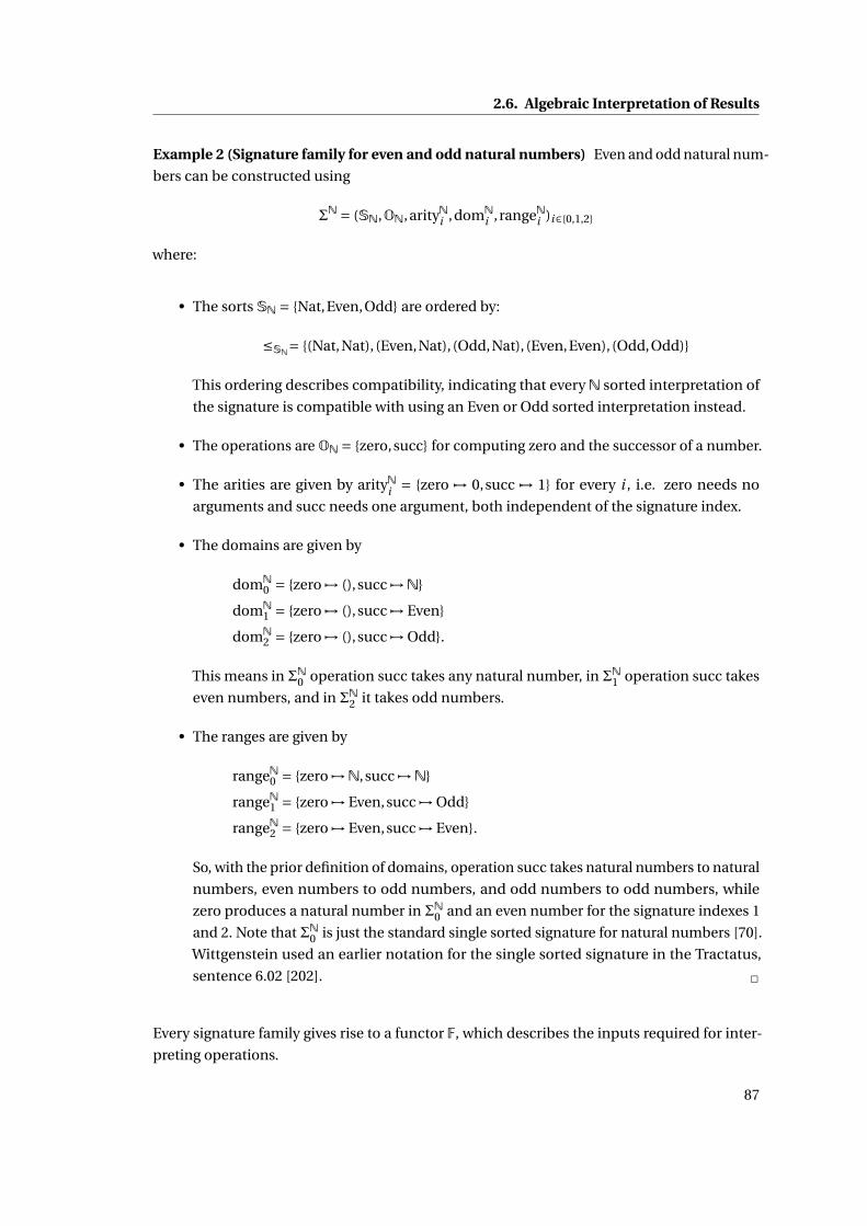
2.6. Algebraic Interpretation of Results
Example 2 (Signature family for even and odd natural numbers) Even and odd natural num-
bers can be constructed using
ΣN = (SN,ON,arityNi ,domNi , rangeNi )i∈{0,1,2}
where:
• The sorts SN = {Nat,Even,Odd} are ordered by:
≤SN= {(Nat,Nat), (Even,Nat), (Odd,Nat), (Even,Even), (Odd,Odd)}
This ordering describes compatibility, indicating that everyN sorted interpretation of
the signature is compatible with using an Even or Odd sorted interpretation instead.
• The operations are ON = {zero,succ} for computing zero and the successor of a number.
• The arities are given by arityNi = {zero ↦→ 0,succ ↦→ 1} for every i , i.e. zero needs no
arguments and succ needs one argument, both independent of the signature index.
• The domains are given by
domN0 = {zero ↦→ (),succ ↦→N}
domN1 = {zero ↦→ (),succ ↦→ Even}
domN2 = {zero ↦→ (),succ ↦→ Odd}.
This means in ΣN0 operation succ takes any natural number, in ΣN1 operation succ takes
even numbers, and in ΣN2 it takes odd numbers.
• The ranges are given by
rangeN0 = {zero ↦→N, succ ↦→N}
rangeN1 = {zero ↦→ Even,succ ↦→ Odd}
rangeN2 = {zero ↦→ Even,succ ↦→ Even}.
So, with the prior definition of domains, operation succ takes natural numbers to natural
numbers, even numbers to odd numbers, and odd numbers to odd numbers, while
zero produces a natural number in ΣN0 and an even number for the signature indexes 1
and 2. Note that ΣN0 is just the standard single sorted signature for natural numbers [70].
Wittgenstein used an earlier notation for the single sorted signature in the Tractatus,
sentence 6.02 [202]. □
Every signature family gives rise to a functor F, which describes the inputs required for inter-
preting operations.
87
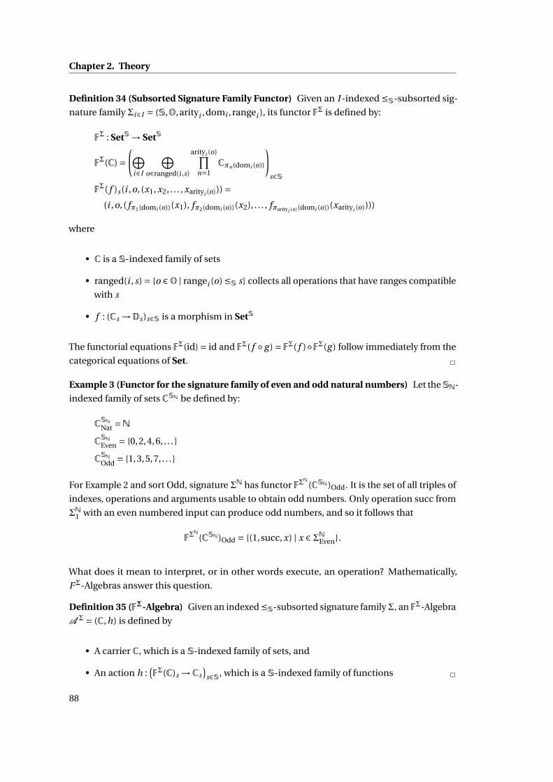
Chapter 2. Theory
Definition 34 (Subsorted Signature Family Functor) Given an I -indexed ≤S-subsorted sig-
nature family Σi∈I = (S,O,arityi ,domi , rangei ), its functor FΣ is defined by:
FΣ : SetS→ SetS
FΣ(C) =(⨁
i∈I
⨁o∈ranged(i ,s)
arityi (o)∏n=1
Cπn (domi (o))
)s∈S
FΣ( f )s(i ,o, (x1, x2, . . . , xarityi (o))) =(i ,o, ( fπ1(domi (o))(x1), fπ2(domi (o))(x2), . . . , fπarityi (o)(domi (o))(xarityi (o))))
where
• C is a S-indexed family of sets
• ranged(i , s) = {o ∈O | rangei (o) ≤S s} collects all operations that have ranges compatible
with s
• f : (Cs →Ds)s∈S is a morphism in SetS
The functorial equations FΣ(id) = id and FΣ( f ◦ g ) = FΣ( f )◦FΣ(g ) follow immediately from the
categorical equations of Set. □
Example 3 (Functor for the signature family of even and odd natural numbers) Let theSN-
indexed family of sets CSN be defined by:
CSNNat =N
CSNEven = {0,2,4,6, . . . }
CSNOdd = {1,3,5,7, . . . }
For Example 2 and sort Odd, signature ΣN has functor FΣN
(CSN)Odd. It is the set of all triples of
indexes, operations and arguments usable to obtain odd numbers. Only operation succ from
ΣN1 with an even numbered input can produce odd numbers, and so it follows that
FΣN
(CSN)Odd = {(1,succ, x) | x ∈ΣNEven}.
What does it mean to interpret, or in other words execute, an operation? Mathematically,
FΣ-Algebras answer this question.
Definition 35 (FΣ-Algebra) Given an indexed ≤S-subsorted signature familyΣ, an FΣ-Algebra
A Σ = (C,h) is defined by
• A carrier C, which is a S-indexed family of sets, and
• An action h :(FΣ(C)s →Cs
)s∈S, which is a S-indexed family of functions □
88

2.6. Algebraic Interpretation of Results
Example 4 (An algebra for the signature family of even and odd natural numbers) Continuing
Example 3, A ΣN
CΣN = (CΣ
N
,hΣN
) is an algebra defined by CΣN
and its action
hΣN
:(FΣ
N
(CΣN
)s →CΣN
s
)s∈S
hΣN
s (i ,zero,()) = 0
hΣN
s (i , succ, x) = x +1
For each index, operation and argument-vector, the action computes the result of inter-
preting that operation. Signatures are interfaces, which can have different implementa-
tions. This is expressed by different algebras for the same signature. An alternative algebra
A ΣN
Mod2 = (Mod2, gΣN
) can be defined by the carrier
Mod2Nat = {0,1} Mod2Even = {0} Mod2Odd = {1}
and action gΣN
:(FΣN(Mod2)s → Mod2s
)s∈S
gΣN
s (i ,zero,()) = 0 gΣN
Nat(0,succ,0) = 1
gΣN
Nat(0,succ,1) = 0
gΣN
Odd(1,succ,0) = 1
gΣN
Even(2,succ,1) = 0
In contrast to A ΣN
CΣN , algebra A ΣN
Mod2 forgets all information about the constructed numbers,
except for their parity. □
The problem of automatic program construction can be reformulated to automatic enumera-
tion of the image of the action of an algebra. Suppose each sort describes a desired program
property, and the carrier set Cs of some FΣ-algebra (C,h) is the set of programs with that
property. Now each operation in Σ is necessarily interpreted by h as a program transformation,
mapping source programs with properties specified by its domain to target programs with the
properties specified by its range. Enumerating the range of hs for a given sort s then produces
all programs with property s that are constructed using the transformations specified inΣ. The
notion of being constructed by operations in Σ is made precise using the following definition.
Definition 36 (Algebraically Generated Objects) Let Σ be an indexed ≤S-subsorted signa-
ture family, and A Σ = (C,h) be an FΣ-algebra. An object is algebraically generated iff it is
contained in any set in the family AlgGenA Σ
. For any sort s, AlgGenA Σ
s ⊆ Cs is the least set
closed under the rule:
If (i ,o, (x1, x2, . . . , xarityi (o))) ∈ FΣ(C)s
and for all i ∈ {1,2, . . . ,arityi (o)} : xi ∈ AlgGenA Σ
πi (domi (o))
then hs(i ,o, (x1, x2, . . . , xarityi (o))) ∈ AlgGenA Σ
s
89

Chapter 2. Theory
2.6.2 Undecidability of Sort Emptiness with infinite Index Sets
The sort emptiness problem of algebraically generated sets is the following: Given an index
set I , an I -indexed ≤S-subsorted signature family Σ, an FΣ-algebra A Σ = (C,h) and a sort s,
is AlgGenA Σ
s =∅? This problem is interesting in two ways: it turns out to be undecidable if
I is an arbitrary set and the undecidability proof is inspired by the undecidability proof for
Combinatory Logic with Hilbert Schematism presented in [163]. The proof idea is to reduce
the halting problem of 2-Counter Automata, which are a well-known Turing complete machine
model [140; 77; 117], to the emptiness problem by equating AlgGenA Σ
s with counter values
for which the configuration represented by s halts. It immediately follows, that enumerating
algebraically generated sets for program construction implicitly includes a programming
language to control the enumeration process – a point which has been made before for
Combinatory Logic [163].
Definition 37 (2-Counter Automata)
Following the definition in [163], a 2-Counter Automaton is defined by (S, s0, s f ,c01 ,c0
2 ,R) where
• S is a finite set of states
• s0 ∈ S is the initial state
• s f ∈ S is the final state
• c01 ,c0
2 ∈N are the initial counter values
• R ⊂R is a finite set of commands for the transition relation drawn from
R ∋ t ::= Addi (s1, s2) | Subi (s1, s2) | Tsti (s1, s2, s3)
with i ∈ {1,2} and s1, s2, s3 ∈ S
Automaton configurations are triples in C = S ×N×N containing a state and two counters.
The transition relation ▷⊂C ×C is the least relation closed under the following rules:
Add1(s1, s2) ∈ R(s1,c1,c2)▷ (s2,c1 +1,c2)
Add2(s1, s2) ∈ R(s1,c1,c2)▷ (s2,c1,c2 +1)
Sub1(s1, s2) ∈ R(s1,c1 +1,c2)▷ (s2,c1,c2)
Sub2(s1, s2) ∈ R(s1,c1,c2 +1)▷ (s2,c1,c2)
Tst1(s1, s2, s3) ∈ R(s1,0,c2)▷ (s2,0,c2)
Tst2(s1, s2, s3) ∈ R(s1,c1,0)▷ (s2,c1,0)
Tst1(s1, s2, s3) ∈ R(s1,c1 +1,c2)▷ (s3,c1 +1,c2)
Tst2(s1, s2, s3) ∈ R(s1,c1,c2 +1)▷ (s3,c1,c2 +1)
The reflexive transitive closure of ▷ is denoted by ▶ and for k ∈C , notation k ▶ is short for
there exists c1,c2 ∈N s.t. k ▶ (s f ,c1,c2). □
90

2.6. Algebraic Interpretation of Results
Definition 38 (Signatures for 2-Counter Automata) For the 2-Counter Automaton A = (S, s0,
s f ,c01 ,c0
2 ,R) signature family Σ2Aut(A) = (SA ,OA ,arityAi ,domA
i , rangeAi )i∈N×N is defined by
• The sorts SA =C = S ×N×N ordered by ≤SA= {(k,k) | k ∈C }
• The operations OA = {s f }⊎ {Addi (s1, s2) | Addi (s1, s2) ∈ R}⊎{Subi (s1, s2) | Subi (s1, s2) ∈ R}⊎{Tst0
n(s1, s2, s3) | Tsti (s1, s2, s3) ∈ R}⊎{Tst+n (s1, s2, s3) | Tsti (s1, s2, s3) ∈ R}
• The arities arityAi (o) =
⎧⎨⎩0 for o = s f
1 otherwise
• The domains domA(c1,c2)(o) =
⎧⎪⎪⎪⎪⎪⎪⎪⎪⎪⎪⎪⎪⎪⎪⎪⎪⎪⎨⎪⎪⎪⎪⎪⎪⎪⎪⎪⎪⎪⎪⎪⎪⎪⎪⎪⎩
() for o = s f
(s2,0,c2) for o = TstZ1 (s1, s2, s3)
(s2,c1,0) for o = TstZ2 (s1, s2, s3)
(s3,c1 +1,c2) for o = Tst+1 (s1, s2, s3)
(s3,c1,c2 +1) for o = Tst+2 (s1, s2, s3)
(s2,c1 +1,c2) for o = Add1(s1, s2)
(s2,c1,c2 +1) for o = Add2(s1, s2)
(s2,c1,c2) for o = Subn(s1, s2)
• The ranges rangeA(c1,c2)(o) =
⎧⎪⎪⎪⎪⎪⎪⎪⎪⎪⎪⎪⎪⎪⎪⎪⎪⎪⎨⎪⎪⎪⎪⎪⎪⎪⎪⎪⎪⎪⎪⎪⎪⎪⎪⎪⎩
(s f ,c1,c2) for o = s f
(s1,0,c2) for o = TstZ1 (s1, s2, s3)
(s1,c1,0) for o = TstZ2 (s1, s2, s3)
(s1,c1 +1,c2) for o = Tst+1 (s1, s2, s3)
(s1,c1,c2 +1) for o = Tst+2 (s1, s2, s3)
(s1,c1,c2) for o = Addn(s1, s2)
(s1,c1 +1,c2) for o = Sub1(s1, s2)
(s1,c1,c2 +1) for o = Sub2(s1, s2)
□
Similar to the type signatures in [163], the idea in the definition of Σ2Aut is to traverse au-
tomaton states backwards from the accepting state s f to the initial state s0. Each possible
automaton transition is implemented by an operation and there exists an additional initial
operation s f without parameters. The signature index controls counter states. Note, that
the sorts SA directly represent automaton configurations without any need for additional
encodings and that no theory of substitutions into sorts is required. This illustrates express-
ibility of native implementation-specific concerns without the requirement of mappings into
approach specific type-structures necessary in [163]. Now an algebra for machine traces can
be constructed.
91

Chapter 2. Theory
Lemma 34 (Machine Trace Algebra) For the 2-Counter Automaton A = (S, s0, s f ,c01 ,c0
2 ,R),
signature family Σ2Aut(A) = (SA ,OA ,arityAi ,domA
i , rangeAi )i∈N×N, and o ∈OA , i ∈N×N, s ∈SA
the following statements are true
1. If o = s f then rangeAi (o)▷domA
i (o)
Define algebra A Σ2Aut(A)
CΣ2Aut(A)
= (CΣ2Aut(A),hΣ
2Aut(A)) with
CΣ2Aut(A)
s = {(c1,c2) ∈N×N | s ▶ (s f ,c1,c2)}
hΣ2Aut(A)
s ((c1,c2),o, x) =⎧⎨⎩(c1,c2) for o = s f
x otherwise
then
2. If exists (c1,c2) ∈CΣ2Aut(A)s0
then (s0,c01 ,c0
2)▶ (s f ,c1,c2)
3. If exists (c1,c2) ∈N×N s.t. (s0,c01 ,c0
2)▶ (s f ,c1,c2) then (c1,c2) ∈ AlgGenA Σ2Aut(A)
CΣ2Aut(A)
s0
PROOF Proposition 1 is proven by case analysis on o matching range and domain with the
rules of ▷. It is used to ensure that hΣ2Aut(A) is well-defined for o = s f . Soundness of the carrier
CΣ2Aut(A) and thereby the algebraically generated set is guaranteed by statement 2, which
immediately follows from the definition of CΣ2Aut(A). Finally, proposition 3 states completeness
and follows by induction on the steps in (s0,c01 ,c0
2)▶ (s f ,c1,c2).
The existence of (c1,c2) ∈ N×N s.t. (s0,c01 ,c0
2) ▶ (s f ,c1,c2) is undecidable and so is the by
statements 2 and 3 equivalent question for emptiness of AlgGenA Σ2Aut(A)
CΣ2Aut(A)
s0. ■
2.6.3 Finite Index Sets and Combinatory Logic
Undecidability for infinite index sets does not render the algebraic approach useless. In
fact, whenever the index set is finite, type inhabitation in FCL can be used to enumerate
AlgGenA Σ
of any algebra A Σ for any signature Σ. The result follows from some abstract
algebraic properties, which require further definitions and proofs. The first two definitions are
extensions of the standard notions for F-CoAlgebras and algebra morphisms [52].
Definition 39 (FΣ-CoAlgebras) Given an indexed ≤S-subsorted signature family Σ, an FΣ-
CoAlgebra A Σ = (C,h) is defined by
• A carrier C, which is a S-indexed family of sets, and
• A co-action h :(Cs → FΣ(C)s
)s∈S, which is a S-indexed family of functions □
92

2.6. Algebraic Interpretation of Results
Definition 40 (Algebra Morphism Families) Given an indexed ≤S-subsorted signature fam-
ily Σ, and FΣ-Algebras A ΣC= (C,h), A Σ
D= (D, g ), family f : (Cs →Ds)s∈I is an algebra morphism
family, if it makes the following diagram commute
FΣ(C)s FΣ(D)s
Cs Ds
hs
FΣ( f )s
gs
fs
i.e. for all s ∈S: fs ◦hs = g ◦FΣ( f )s □
The next lemma extends the work of Paulson [154] to structures with polymorphic indexes.
Lemma 35 (Well-Founded Fixpoint Families) Let M be a set and R ⊆ M×M be a well-founded
relation (c.f. Lemma 31). Remember that the accessibility predicate of R is the least predicate
closed under rule:
for all y: if R(y, x) then Acc(y)Acc(x)
For any y s.t. R(y, x), let Acc−1x (ax , y) be the proof tree of Acc(y) in the premise of any given proof
tree ax of Acc(x) . Observe that the proof tree Acc−1x (ax , y) is always strictly smaller than the
proof tree ax .
Given an index set S, an S-indexed family of sets C, a family of sets P indexed over members of
C, and a measuring map m :∏
s∈SCs → M, define for all s1, s2 ∈S and x ∈Cs1 :
↓ (x, s2) = {y ∈Cs2 | R(m(s2, y),m(s1, x))}
Then given a morphism F :∏
s1∈S∏
x∈Cs1
(∏s2∈S
∏y∈↓(x,s2) Py
)→ Px the fixpoint morphism
FixAccF :∏s∈S
∏x∈C
Acc(m(s, x)) → Px
FixAccF (s1, x, am(s1,x)) = F (s1, x,λ(s2, y).FixF (s2, y,Acc−1m(s1,x)(am(s1,x),m(s2, y))))
can be constructed because of the prior observation on proof tree sizes.
F is extensional in its third argument if for all s1 ∈S, x ∈Cs1 , and g , g ′ :∏
s2∈S∏
y∈↓(x,s2) Py , s.t.
for all s2 ∈S, and y ∈Cs2 : g (s2, y) = g ′(s2, y), the statement F (s1, x, g ) = F (s2, x, g ′) is true. This
always holds in extensional set-theory, but has to be shown on a per-case basis in intensional
type theory.
93

Chapter 2. Theory
For any F that is extensional in its third argument, s1 ∈S, x ∈Cs1 , proof trees am(s1,x), a′m(s1,x) of
Acc(m(s1, x)), and morphisms G :∏
s∈S∏
y∈CsPy morphism FixAccF is:
1. Invariant in its proof tree argument: FixAccF (s1, x, am(s1,x)) = FixAccF (s1, x, a′m(s1,x))
2. A unique solution to the fixpoint equation: if for all s2 ∈S, y ∈Cs2 : G(s2, y) = F (s2, y,G)
then FixAccF (s1, x, am(s1,x)) =G(s1, x)
This justifies to write
Fix(F )(s, x) = FixAccF (s, x, am(s,x)) = F (s, x,Fix(F ))
where am(s,x) is any proof tree of Acc(m(s, x)) and always exists because R is well-founded. It
also yields the well-founded family induction principle:
If for all s1, x :
if for all s2, y : R(m(s2, y),m(s1, x)) implies Q(y)
then Q(x)
then forall s, x : Q(x)
where Q is a predicate on elements of C.
PROOF Statements 1 and 2 are both proven by using the well-founded induction principle (c.f.
Lemma 31) on am(s,x) and then follow by simple unfolding of definitions. In the constructive
logic of Coq, the well-founded family induction principle exists because propositions are
types and recursion and induction coincide. In classical logic the principle is generated
by instantiating Fix with P = ({y ∈ Cs | y = x and Q(y)}x∈Cs )s∈S and F (s, x, f ) = x. Whenever
F has a non-empty domain, its argument f exists. Now for any given s1, x and s2, y with
R(m(s2, y),m(s1, x)), f computes an element of P , which implies Q(y). Therefore the induction
hypothesis is applicable, and Q(x) is true, which means x is an element of P . Thus F is well-
defined and existence of Fix(F )(s, x) as an element of P proves Q(x). ■
Lemma 36 (Canonical Algebra Morphism) Given an I -indexed ≤S-subsorted signature fam-
ily Σ, FΣ-Algebras A Σ1 = (C,h), A Σ
2 = (C, g ), FΣ-CoAlgebra A Σ1 = (C,h−1), a set M, well-founded
relation R ⊆ M ×M, and a measuring map m :∏
s∈SCs → M decreasing on h−1 s.t.
for all s ∈S, x ∈Cs , (i ,o,args) = h−1s (x),n ∈ 1,2, . . . ,arityi (o) :
R(m(πn(domi (o)),πn(args)),m(s, x))
define the canonical algebra morphism family
interpret : (Cs →Ds)s∈Sinterprets(x) = Fix(λ(s, x, f ).(gs ◦FΣ( f )s ◦h−1
s )(x))(s, x)
94
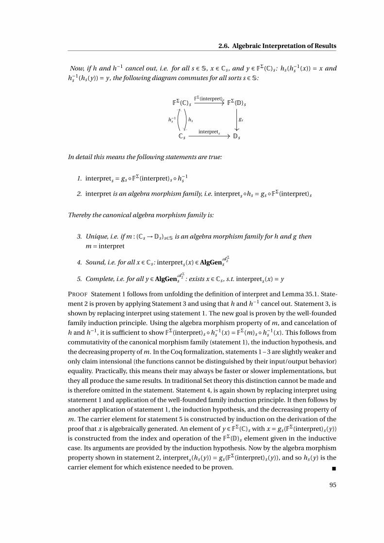
2.6. Algebraic Interpretation of Results
Now, if h and h−1 cancel out, i.e. for all s ∈ S, x ∈ Cs , and y ∈ FΣ(C)s : hs(h−1s (x)) = x and
h−1s (hs(y)) = y, the following diagram commutes for all sorts s ∈S:
FΣ(C)s FΣ(D)s
Cs Ds
hs
FΣ(interpret)s
gsh−1s
interprets
In detail this means the following statements are true:
1. interprets = gs ◦FΣ(interpret)s ◦h−1s
2. interpret is an algebra morphism family, i.e. interprets ◦hs = gs ◦FΣ(interpret)s
Thereby the canonical algebra morphism family is:
3. Unique, i.e. if m : (Cs →Ds)s∈S is an algebra morphism family for h and g then
m = interpret
4. Sound, i.e. for all x ∈Cs : interprets(x) ∈ AlgGenA Σ
2s
5. Complete, i.e. for all y ∈ AlgGenA Σ
2s : exists x ∈Cs , s.t. interprets(x) = y
PROOF Statement 1 follows from unfolding the definition of interpret and Lemma 35.1. State-
ment 2 is proven by applying Statement 3 and using that h and h−1 cancel out. Statement 3, is
shown by replacing interpret using statement 1. The new goal is proven by the well-founded
family induction principle. Using the algebra morphism property of m, and cancelation of
h and h−1, it is sufficient to show FΣ(interpret)s ◦h−1s (x) = FΣ(m)s ◦h−1
s (x). This follows from
commutativity of the canonical morphism family (statement 1), the induction hypothesis, and
the decreasing property of m. In the Coq formalization, statements 1 – 3 are slightly weaker and
only claim intensional (the functions cannot be distinguished by their input/output behavior)
equality. Practically, this means their may always be faster or slower implementations, but
they all produce the same results. In traditional Set theory this distinction cannot be made and
is therefore omitted in the statement. Statement 4, is again shown by replacing interpret using
statement 1 and application of the well-founded family induction principle. It then follows by
another application of statement 1, the induction hypothesis, and the decreasing property of
m. The carrier element for statement 5 is constructed by induction on the derivation of the
proof that x is algebraically generated. An element of y ∈ FΣ(C)s with x = gs(FΣ(interpret)s(y))
is constructed from the index and operation of the FΣ(D)s element given in the inductive
case. Its arguments are provided by the induction hypothesis. Now by the algebra morphism
property shown in statement 2, interprets(hs(y)) = gs(FΣ(interpret)s(y)), and so hs(y) is the
carrier element for which existence needed to be proven. ■
95

Chapter 2. Theory
At this point, category theory proficient readers will find Lemma 36 reminiscent of Lambek’s
Lemma [121] and its applications [84]. However, the construction does the opposite. Lambek’s
Lemma proves that functors with an initial algebra (there is a unique algebra morphism to any
other algebra) are fixpoints [1]. Here, conversely, a (family of) fixpoint(s) is used to prove that a
given algebra is initial by providing the (family of) canonical algebra morphism(s). The algebra
is chosen to have terms typable by Combinatory Logic as its carrier, and the algebra morphism
translates them to terms of any algebraically generated language. Meyer [138] clarifies the
notion of models for Combinatory Logic with combinators S and K as their base. Inversely,
the next construction finds a base for a given model (signature and algebra).
Lemma 37 (Finite Combinatory Logic (Co)Algebra) Given a ≤S-subsorted signature family
Σi∈I = (S,O,arityi ,domi , rangei ) indexed over a finite set I , define:
• The set of applicative terms A formed over combinator base B ∋ x ::= o | idxi for all i ∈ I
and o ∈O
• The set of types intersection types T formed over constructors C ∋ c ::= s | idxi for all i ∈ I
and s ∈S preordered by ≤C=≤S ⊎{(idxi , idxi ) | i ∈ I }
• The index context ΓI : I →T by ΓI (i ) = idxi (ω)
• The sort embedding function embed :S→T by embed(s) = s(ω)
• The sort unembedding function unembed(A) =⎧⎨⎩(1, s) for A = s(ω) and s ∈S
(0, ()) otherwise
• Function typeAtIndex :O× I →T by
typeAtIndex(o, i ) =ΓI (i ) → mkArrow(rev(map(λn.embed(πn(domi (o))),enum({1,2, . . . ,arityi (o)}))),
embed(rangei (o)))
• Function ΓΣ :O→T by ΓΣ(o) =⋂i∈enum(I ) typeAtIndex(o, i )
• Context Γ : B →T by Γ(x) =⎧⎨⎩ΓI (i ) for x = idxi
ΓΣ(x) otherwise
• The Combinatory Logic carrier Cs = {M ∈A | Γ⊢ M : embed(s)}
• The Combinatory Logic FΣ-Algebra A ΣFCL = (Cs ,h) with action
hs(i ,o,args) = revApply(@(o, idxi ), rev(map(λn.πn(args),enum({1,2, . . . ,arityi (o)}))))
96

2.6. Algebraic Interpretation of Results
• The Combinatory Logic FΣ-CoAlgebra A ΣFCL = (Cs ,h) with co-action
h−1s (M) = (i ,o, (arg1,arg2, . . . ,argarityi (o)))
for unapply(M) = (o, N s) and rev(N s) = [:: idxi &[:: arg1 &[:: arg2 &.. . [::arityi (o)]]]]
Which is possible because the following statements are true for all i ∈ I , o ∈O, and s, s1, s2 ∈S,
M ∈A, and N s, N s′ ∈A∗, Ms ∈Cs , t ∈ FΣ(C)s , and A1, A2 ∈T, and c1,c2 ∈ C, and srcs1, srcs2 ∈T∗π:
1. unembed(embed(s)) = (1, s)
2. If s1 ≤S s2 then embed(s1) ≤ embed(s2)
3. Γ⊢ hs(t ) : embed(s)
4. unapply(Ms).1 = idxi
5. If mkArrow(srcs2,c2(A2)) ≤ mkArrow(srcs1,c1(A1)) then
c2(A2) ≤ c1(A1) and lsize(srcs1) = lsize(srcs2) and
for all (src1, src2) in zip(srcs1, srcs2): src1 ≤ src2
6. If Γ⊢ M : idxi (ω) then M = idxi
7. If rev((unapply(Ms)).2) = [:: N &N s] then there exists i ∈ I s.t. N = idxi
8. If unapply(Ms) = (o, N s) and rev(N s) = [:: idxi &N s′] then lsize(N s′) = arityi (o)
9. If unapply(Ms) = (o, N s) and rev(N s) = [:: idxi &N s′] then
for all 1 ≤ n ≤ lsize N s′: Γ⊢ nth(N s′,n −1) :πn(domi (o))
10. If unapply(Ms) = (o, N s) and rev(N s) = [:: idxi &N s′] then rangei (o) ≤S s
PROOF Statements 1 and 2 immediately follow from the definitions. Statement 3 guarantees
that the algebra action hs is well-defined and follows from the subtype rule (≤) of FCL Def-
inition 12 and generalized application (Lemma 15.1). The other statements are required to
ensure that the co-action h−1s is well defined. Statement 4 follows from inverse application
(Lemma 15.2), minimal type correctness (Lemma 16), subtype machine corretness (Theo-
rem 1), and case-analysis on the subtype machine rules (Definition 5). The proof of statement
5 is by inverse induction on the sources srcs1 and srcs2, again followed by case-analysis on
the subtype machine rules. Statement 6 is shown by normalized induction (Lemma 10) on
the derivation and inverse application, minimal type correctness, primality (c.f. Lemma 8)
of types in Γ, and statement 5 are used to discharge the applicative case. An analogous proof
is used for statements 7, just with inverse application instead of normalized induction. This
is repeated for the other statements 8–10, additionally using statements 4 and 7 in inverse
induction on N s followed by inverse induction on the types obtained by applying the inverse
application lemma. ■
97

Chapter 2. Theory
It remains to show, that A ΣFCL and A Σ
FCL give rise to a canonical algebra morphism family into
any other algebra.
Lemma 38 (Finite Combinatory Logic Algebra Morphism Conditions) For A ΣFCL and A Σ
FCL
from Lemma 37 define the forgetful measure map
measureFCL :∏s∈S
Cs →A
measureFCL(s, M) = M
and the least relation IsChild ⊂A×A closed under rule
M is in (unapply(N )).2
IsChild(M , N )
Then for all predicates P on applicative terms, M ∈ A, s ∈ S, Ms ∈ Cs , o ∈ O, i ∈ I ,
xs ∈∏arityi (o)n=1 πn(domi (o)), and t ∈ FΣ(C)s the following statements are true:
1. If for all c ∈ B and N s in A∗ :
for all N in N s : P (N )implies P (revApply(c, N s))
then P (M)
2. Relation IsChild is well-founded: WF(IsChild)
3. If h−1s (Ms) = (i ,o, xs) then
IsChild(measureFC L(πn(domi (o)),πn(xs)),measureFC L(s, Ms))
4. h−1s (hs(t )) = t
5. hs(h−1s (Ms)) = Ms
PROOF Statement 2 is an induction principle on applicative terms, which is proven by rewrit-
ing the result P (M) to P (revApply(M , [::])) using Lemma 14.2 and then generalizing to "if N
in [::] implies P (N ), then P (revApply(M , [::]))" and further to "if N in N s implies P (N ), then
P (revApply(M , N s))" for arbitrary N s ∈A∗. Induction on M is now enough to show the result,
using Lemma 14.1 in the case for applications. Statement 2 easily follows from the induc-
tion principle in statement 2 and Lemma 14.3. The other statements follow by unfolding
the definition of the (co-)action with an additional inverse induction on N s computed by
h−1s (Ms) = (i ,o, N s) to prove the last statement. ■
With the measure map into the well-founded IsChild relation and the cancelation properties,
everything is set up to show the final theorem about uniqueness, soundness and completeness
of the translation from Combinatory Logic into the algebraically generated set of any given
algebra for any given signature.
98
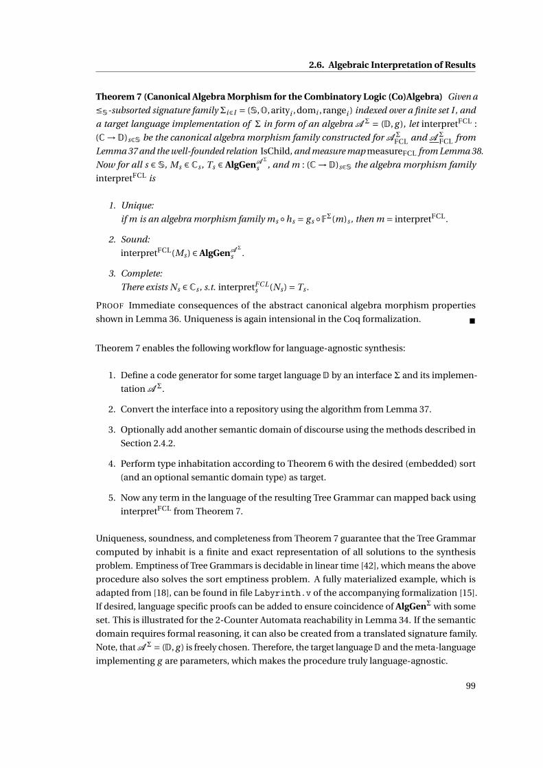
2.6. Algebraic Interpretation of Results
Theorem 7 (Canonical Algebra Morphism for the Combinatory Logic (Co)Algebra) Given a
≤S-subsorted signature family Σi∈I = (S,O,arityi ,domi , rangei ) indexed over a finite set I , and
a target language implementation of Σ in form of an algebra A Σ = (D, g ), let interpretFCL :
(C→D)s∈S be the canonical algebra morphism family constructed for A ΣFCL and A Σ
FCL from
Lemma 37 and the well-founded relation IsChild, and measure map measureFCL from Lemma 38.
Now for all s ∈S, Ms ∈ Cs , Ts ∈ AlgGenA Σ
s , and m : (C→D)s∈S the algebra morphism family
interpretFCL is
1. Unique:
if m is an algebra morphism family ms ◦hs = gs ◦FΣ(m)s , then m = interpretFCL.
2. Sound:
interpretFCL(Ms) ∈ AlgGenA Σ
s .
3. Complete:
There exists Ns ∈Cs , s.t. interpretFC Ls (Ns) = Ts .
PROOF Immediate consequences of the abstract canonical algebra morphism properties
shown in Lemma 36. Uniqueness is again intensional in the Coq formalization. ■
Theorem 7 enables the following workflow for language-agnostic synthesis:
1. Define a code generator for some target language D by an interface Σ and its implemen-
tation A Σ.
2. Convert the interface into a repository using the algorithm from Lemma 37.
3. Optionally add another semantic domain of discourse using the methods described in
Section 2.4.2.
4. Perform type inhabitation according to Theorem 6 with the desired (embedded) sort
(and an optional semantic domain type) as target.
5. Now any term in the language of the resulting Tree Grammar can mapped back using
interpretFCL from Theorem 7.
Uniqueness, soundness, and completeness from Theorem 7 guarantee that the Tree Grammar
computed by inhabit is a finite and exact representation of all solutions to the synthesis
problem. Emptiness of Tree Grammars is decidable in linear time [42], which means the above
procedure also solves the sort emptiness problem. A fully materialized example, which is
adapted from [18], can be found in file Labyrinth.v of the accompanying formalization [15].
If desired, language specific proofs can be added to ensure coincidence of AlgGenΣ with some
set. This is illustrated for the 2-Counter Automata reachability in Lemma 34. If the semantic
domain requires formal reasoning, it can also be created from a translated signature family.
Note, that A Σ = (D, g ) is freely chosen. Therefore, the target languageD and the meta-language
implementing g are parameters, which makes the procedure truly language-agnostic.
99

Chapter 2. Theory
100

Chapter 3
The (CL)S Framework
The (CL)S Framework implements the theoretical results described in Section 2. At the time of
writing the framework has been under development for over 7 years. The earliest prototype
has been implemented in Prolog and a subsequent incarnation was ported to F#, mainly for
performance and maintainability reasons [56; 55]. This implementation has been continued
evaluating multiple ideas including availability as a web-service and modal intersection types
[59; 20]. Dudenhefner [61] describes the development of its latest incarnation, cls-fsharp [62],
with a focus on performance optimizations, mainly by making smart choices when substituting
type variables, implementing and extending the theoretical results presented in [58; 67]. The
ideas presented in [20] also lead to another branch of development, cls-scala [111], that is
implemented in Scala and described in this section. In contrast to cls-fsharp, which is built for
evaluating performance gains from different inhabitation strategies, its focus is on practical
concerns of software composition synthesis. These include an embedded domain specific
language (EDSL) to develop components, built-in support for automatically translating and
executing synthesized applicative terms, features to enable language-independent meta-
programming, versioned hosting of synthesized artifacts, seamless integration into the Scala
ecosystem via standard build-system dependencies, model driven development capabilities,
and most recently [18] the capability to visually inspect the synthesis process in order to debug
specifications. The architecture of cls-scala is modular and separated into multiple projects.
It is described in Section Section 3.1. All of its components are open source and available
online together with evolving ecosystem of related projects [27]. Notably, some of these just
make use of the metaprogramming features without using inhabitation, e.g. EpCoGen [97],
a framework for generating and studying approaches to solve the expression problem [199].
The extension to Scala with an EDSL for specifying software components (Section 3.2), meta-
programming support mechanisms and features for versioned artifact hosting have been
developed (Section 3.3) in step with the requirements arising from work on software product
lines [96; 21; 60; 95; 164]. The implementation is closely connected to its theory described in
Chapter 2 and accompanied by a suite of tests is described in Section 3.4. Finally it should
not go unmentioned that the proven Coq formalization [15] of Chapter 2 can be extracted
101

Chapter 3. The (CL)S Framework
to executable Haskell or OCaml code. It can thus serve as a verified baseline to investigate
future bugs of cls-scala. Additionally, if an increased level of confidence is required for some
application, it can be used to formally prove correctness of synthesis results.
The Coq formalization is an independent work of the author of this text. Most code of the
cls-scala framework has been created by the author, with some contributions from others.
The most notable other direct contributors of source code are George T. Heineman and Anna
Vasileva. Many design decisions were also made in team with Boris Düdder, whose prior
experience developing earlier versions of the framework was invaluable. All projects are
publicly available [27] and their source commit history can be traced author by author.
102

3.1. Architecture Overview
3.1 Architecture Overview
AST ManipulationCombinators
AST Node Type andSemantic Concept Generated Code
Signature andImplementation
Repository(Type Context)
Request for Scala- andSemantic Type
Tree Grammar Stream ofTrees
Stream ofValues
Website andGit Branches
Framework
Application
reflection reflection
typeinhabitation
enumerationusing FEAT
runtimecompilation
presentationto user
Figure 3.1: Data flow in cls-scala
Figure 3.1 shows the typical data flow when using cls-scala. An application implements com-
ponents in Scala as combinators that provide or manipulate fragments of abstract syntax trees
(ASTs) of a target language. Problem instance specific boxes are drawn in white: combinators
can manipulate any Scala objects, and ASTs are just one use-case that is often encountered.
The signature of components and their semantic types are collected using reflection and
translated into a single type context. A request is made, typically for the type of an AST node
and a semantic type. Type inhabitation creates a Tree Grammar describing all applicative
solution terms. The Tree Grammar is enumerated as a continuous stream of data using the
functional enumeration of algebraic types (FEAT) technique by Duregård et al. [68]. Upon re-
quest each inhabitant is translated to Scala using the canonical algebra morphism constructed
in Section 2.6.3. The translated term is then runtime-compiled and injected back into the
JVM where it is executed. Results are available as a stream. If the results can be serialized,
infrastructure is provided to store them in a Git [189] repository and to inspect and control
their creation via a website.
cls-scala cls-scala-presentation-play-git cls-scala-templating
shapeless-feat
Figure 3.2: Projects in the cls-scala framework and their dependencies
Figure 3.2 shows the main projects of the framework with arrows indicating their interdepen-
dencies. Stages above the dotted line of Figure 3.1 are implemented in the cls-scala project. Its
implementation of FEAT is separated into a different project. The shapeless-feat project is a
port of the original Haskell library [68] with additional integration into the shapeless frame-
work [169], which provides data-type generic programming [128] features beyond the scope
103

Chapter 3. The (CL)S Framework
of this text. Separation into a different project enables reuse independent of (CL)S. Similarly,
the template-based metaprogramming infrastructure is provided as a separate project. Type
inhabitation and its algebraic interpretation works independently of any metaprogramming
support, so there is no direct dependency of cls-scala on cls-scala-templating. Vice versa, the
templating support is generic enough not to depend on cls-scala. If results are source code
artifacts that can be serialized to disk, the cls-scala-presentation-play-git project can host
them. It uses the Play framework [33] and its integrated web-server to present users with a
website to manage repositories. Git access and hosting is provided using EGit [203].
All projects are built using the sbt build system [93]. Continuous integration provided by
Travis [80] automatically builds each project, executes its test-suite and triggers the early
release [198] build target. This pushes a snapshot of every successfully tested master branch
commit to maven central [11], from where the project can be immediately included as a jar-file
dependency into other projects. The sbt build system has cross building support to create,
test and publish jar-files for different Scala versions. At the time of writing Scala 2.11 and 2.12
are supported. The coveralls service [137] automatically collects test coverage reports from
each build and publishes them with a detailed analysis.
The Software and sources are released under a permissive open source Apache 2 license [4].
This allows free and commercial, open and closed-source projects to include all or parts of the
software with limited warranty, liability and possibility of patent-claims against the authors.
104
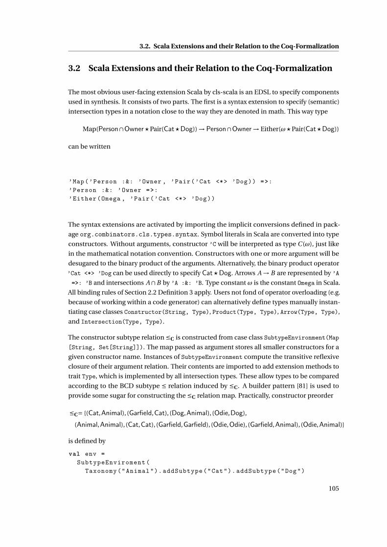
3.2. Scala Extensions and their Relation to the Coq-Formalization
3.2 Scala Extensions and their Relation to the Coq-Formalization
The most obvious user-facing extension Scala by cls-scala is an EDSL to specify components
used in synthesis. It consists of two parts. The first is a syntax extension to specify (semantic)
intersection types in a notation close to the way they are denoted in math. This way type
Map(Person∩Owner⋆Pair(Cat⋆Dog)) →Person∩Owner→ Either(ω⋆Pair(Cat⋆Dog))
can be written
’Map(’Person :&: ’Owner , ’Pair(’Cat <∗> ’Dog)) =>:’Person :&: ’Owner =>:’Either (Omega , ’Pair(’Cat <∗> ’Dog))
The syntax extensions are activated by importing the implicit conversions defined in pack-
age org.combinators.cls.types.syntax. Symbol literals in Scala are converted into type
constructors. Without arguments, constructor ’C will be interpreted as type C (ω), just like
in the mathematical notation convention. Constructors with one or more argument will be
desugared to the binary product of the arguments. Alternatively, the binary product operator
’Cat <∗> ’Dog can be used directly to specify Cat⋆Dog. Arrows A → B are represented by ’A=>: ’B and intersections A∩B by ’A :&: ’B. Type constant ω is the constant Omega in Scala.
All binding rules of Section 2.2 Definition 3 apply. Users not fond of operator overloading (e.g.
because of working within a code generator) can alternatively define types manually instan-
tiating case classes Constructor(String, Type), Product(Type, Type), Arrow(Type, Type),
and Intersection(Type, Type).
The constructor subtype relation ≤C is constructed from case class SubtypeEnvironment(Map[String, Set[String]]). The map passed as argument stores all smaller constructors for a
given constructor name. Instances of SubtypeEnvironment compute the transitive reflexive
closure of their argument relation. Their contents are imported to add extension methods to
trait Type, which is implemented by all intersection types. These allow types to be compared
according to the BCD subtype ≤ relation induced by ≤C. A builder pattern [81] is used to
provide some sugar for constructing the ≤C relation map. Practically, constructor preorder
≤C= {(Cat,Animal), (Garfield,Cat), (Dog,Animal), (Odie,Dog),
(Animal,Animal), (Cat,Cat), (Garfield,Garfield), (Odie,Odie), (Garfield,Animal), (Odie,Animal)}
is defined by
val env =SubtypeEnviroment (
Taxonomy (" Animal "). addSubtype ("Cat"). addSubtype ("Dog")
105

Chapter 3. The (CL)S Framework
.merge( Taxonomy ("Cat"). addSubtype (" Garfield "))
.merge( Taxonomy ("Dog"). addSubtype ("Odie")). underlyingMap )
after which variable results in
import env._val results =
(’Pair(’Garfield <∗> ’Odie). isSubtypeOf (’Pair(’Cat <∗> Animal )),’Pair(’Garfield <∗> ’Odie)
. isSupertypeOf (’Pair(’Animal <∗> Animal )))
contains (true, false). The subtype algorithm is implemented using the machine from
Section 2.3 Definition 9.
The Scala implementation allows for finite type schematism. Types are extended with variables
and a finite set of well-formed substitutions is declared. When a combinator uses ownerTypedeclared in
val alpha = Variable ("alpha")val beta = Variable ("beta")val substitutionSpace =
Kinding (alpha). addOption (’Garfield ). addOption (’Odie).merge( Kinding (beta). addOption (’Jon))
val ownerType = ’FeedsWithLasagna (alpha , beta)
its use will be expanded to
’FeedsWithLasagna (’Garfield , ’Jon):&: ’FeedsWithLasagna (’Odie , ’Jon)
Well-formed substitution spaces can be any finite collection of Scala functions Variable =>Type and Kinding again implements a builder pattern to simplify their construction.
The most basic way to perform type inhabitation is to use an instance of InhabitationAlgorithmaccording to the following type definitions from package org.combinators.cls.inhabitation
type Repository = Map[String , Type]type TreeGrammar = Map[Type , Set [( String , Seq[Type ])]]type InhabitationAlgorithm =
( FiniteSubstitutionSpace , SubtypeEnvironment , Repository ) =>Seq[Type] => TreeGrammar
Inhabitation algorithms take a finite substitution space, a subtype environment, a repository,
and a sequence of types to inhabit. They then produce a Tree Grammar representing all
requested inhabitants. Substitutions spaces and subtype environments have been described
before. Repositories are just maps assigning each combinator a type. In contrast to the Coq
formalization, Tree Grammars in the Scala implementation use uncurried representations
106

3.2. Scala Extensions and their Relation to the Coq-Formalization
(c(M , N ) instead of @(@(c, M), N )) of applicative terms. This is equivalent except for target
type ω, which cannot be represented. Behavior of the Scala implementation is, at the time
of writing, undefined for this case, which is rare enough that it only became apparent during
the rigorous formalization. The Scala implementation can schedule multiple inhabitation
targets in a batch job, resulting in one big Tree Grammar. This is justified by Section 2.5
Lemma 29.5, and the various weakening properties in Lemma 33. It can lead to perfor-
mance improvements, if the recursive target types in batched inhabitation requests overlap,
allowing the algorithm to reuse parts of the previously constructed Tree Grammar. There
are two implementations of type InhabitationAlgorithm, both contained in package org.combinators.cls.inhabitation. The first one by class BoundedCombinatoryLogic performs
all substitutions and then dispatches to the second one by class FiniteCombinatoryLogic,
which performs inhabitation for a context without type variables. Implementations of splitTy
(c.f. Section 2.5 Definition 26) and the cover machine (c.f. Section 2.5 Definition 21) match
the Coq formalization up to minor language differences. The function for inhabitation_step,
additionally to using uncurried applicative terms, accumulates covers (c.f. Section 2.5 Defi-
nition 29) for multiple combinators in parallel by turning the foldl into a map-reduce [122]
operation. The resulting performance benefit has been discussed at length by Düdder [55] and
Scala has parallel collections in its standard library [161], which allow the algorithm to be kept
almost unchanged. The implementation as a state machine operating with single invocations
of inhabitation_step makes it possible to debug the inhabitation process for a given repository
in order to find out, which targets are dropped for being uninhabited. See [18] for a detailed
description of a debugger implemented on top of cls-scala.
The extensions described up to this point are similar to the capabilities of cls-fsharp and earlier
incarnations of the (CL)S framework. The cls-scala implementation is made unique by the
second extension, which builds upon the algebraic theory of Section 2.6. It allows to specify
Section 2.4.2 Example 1 as shown in Listing 3.1.
1 class MotivationRepository {2 val performer : Variable = Variable (" performer ")3 val defaultPerformerSpace =4 Kinding ( performer ). addOption (’Springsteen )5
6 @ combinator object motivationSong {7 def apply (): LilyPond [Music] =8 LilyPond . loadMusic (" noretreat .ly")9 val semanticType : Type = ’Springsteen
10 }11 @ combinator object addLyrics {12 def apply(music: LilyPond [Music],13 lyrics : String ): LilyPond [Song] =14 music. setLyrics ( lyrics )15 val semanticType : Type = performer =>: performer =>: performer16 }17 class LyricsCombinator ( lyrics : String , performerName : String ) {
107
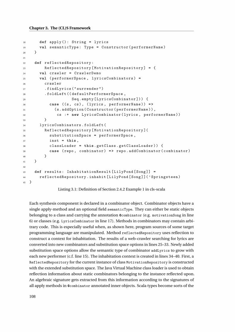
Chapter 3. The (CL)S Framework
18 def apply (): String = lyrics19 val semanticType : Type = Constructor ( performerName )20 }21
22 def reflectedRepository :23 ReflectedRepository [ MotivationRepository ] = {24 val crawler = CrawlerDemo25 val ( performerSpace , lyricsCombinators ) =26 crawler27 . findLyrics (" surrender ")28 . foldLeft (( defaultPerformerSpace ,29 Seq.empty[ LyricsCombinator ])) {30 case ((s, cs), (lyrics , performerName )) =>31 (s. addOption ( Constructor ( performerName )),32 cs :+ new LyricsCombinator (lyrics , performerName ))33 }34 lyricsCombinators . foldLeft (35 ReflectedRepository [ MotivationRepository ](36 substitutionSpace = performerSpace ,37 inst = this ,38 classLoader = this. getClass . getClassLoader )) {39 case (repo , combinator ) => repo. addCombinator ( combinator )40 }41 }42
43 def results : InhabitationResult [ LilyPond [Song ]] =44 reflectedRepository . inhabit [ LilyPond [Song ]]( ’Springsteen )45 }
Listing 3.1: Definition of Section 2.4.2 Example 1 in cls-scala
Each synthesis component is declared in a combinator object. Combinator objects have a
single apply-method and an optional field semanticType. They can either be static objects
belonging to a class and carrying the annotation @combinator (e.g. motivationSong in line
6) or classes (e.g. LyricsCombinator in line 17). Methods in combinators may contain arbi-
trary code. This is especially useful when, as shown here, program sources of some target
programming language are manipulated. Method reflectedRepository uses reflection to
construct a context for inhabitation. The results of a web-crawler searching for lyrics are
converted into new combinators and substitution space options in lines 25–33. Newly added
substitution space options allow the semantic type of combinator addLyrics to grow with
each new performer (c.f. line 15). The inhabitation context is created in lines 34–40. First, a
ReflectedRepository for the current instance of class MotivationRepository is constructed
with the extended substitution space. The Java Virtual Machine class loader is used to obtain
reflection information about static combinators belonging to the instance reflected upon.
An algebraic signature gets extracted from this information according to the signatures of
all apply methods in @combinator annotated inner objects. Scala types become sorts of the
108

3.2. Scala Extensions and their Relation to the Coq-Formalization
C InhabitationResultT
grammar : TreeGrammartarget : Type
resultInterpreter : Tree =>Tterms : feat.Enumeration[Tree]interpretedTerms: feat.Enumeration[T]
InhabitationResult(grammar: TreeGrammar, target: Type, resultInterpreter: Tree =>T)isEmpty : BooleanisInfinite : Booleansize : Option[BigInt]
Figure 3.3: Class to encapsulate inhabitation results
signature, which are ordered by their language native subtype relation. Additionally, the
semantic type information is included (Section 2.4.2 explains how and why native and se-
mantic types may be freely mixed). If required, semantic types can also be ordered by a
subtype environment passed to the ReflectedRepository constructor. Webcrawler results
cannot be known statically at compile time. Their combinators are added dynamically to
the repository at run time (line 39). Signature operations for static combinators are just their
object names, while dynamic combinators are suffixed with a unique identifier, which al-
lows to have multiple instances of the same class inserted as multiple different combinators.
Standard Scala objects and classes are used for component specifications. Therefore, combi-
nator implementations can be shared using inheritance and other object-oriented features,
and the learning curve for users not familiar with algebra or Combinatory Logic is reduced.
Line 44 shows the request for all inhabitants that have native type LilyPond[Song] and the
semantic type Springsteen. Results are encapsulated in class InhabitationResult shown in
Figure 3.3. It includes the Tree Grammar, the requested target type, and in the constructor
ReflectedRepository also passes the canonical algebra morphism for Combinatory Logic
(Section 2.6 Theorem 7), which translates applicative Terms of type Tree to the native type
T. The Scala algebra for this morphism is implemented by creating calls to the combinator
objects collected by ReflectedRepository. Code for these calls is compiled, injected back into
the class loader and then executed. Field InhabitationResult.terms stores a lazily computed
enumeration of all terms that are words of the Tree Grammar for the target non-terminal (c.f.
Section 2.5.2 Definition 28). Terms in this enumeration are ordered ascending by their number
of terminal symbols. The InhabitationResult.interpretedTerms field stores the result of
lazily mapping the translation to Scala over InhabitationResult.interpretedTerms. Addi-
tionally, the class offers methods to check if the Tree Grammar is empty, infinite, or if it is finite
to compute the number of results. See [42] for the algorithms used in these computations.
109

Chapter 3. The (CL)S Framework
3.3 Metaprogramming Support Mechanisms
C Java
fullText: String
compilationUnit(): CompilationUnitstatement(): Statementexpression[T <: Expression](): Ttpe(): Type...
I«trait»
Persistable
type T
rawText(elem: T): Array[Byte]path(elem: T): PathfullPath(basePath: Path, elem: T): PathpersistOverwriting(basePath: Path, elem: T): Filepersist(basePath: Path, elem: T): File
«object»
Java
apply(source: String): Java
Figure 3.4: Main components of project templating for target language Java
The templating project adds lightweight metaprogramming support. Figure 3.4 shows the
main components for this (exemplified for the target language Java). Class Java is a wrapper
around a string to provide extension methods to invoke a parser. They are implemented
using the JavaParser project [195], which offers parsing, pretty printing and AST manipulation
support for Java. The most useful syntactic sorts in the AST are accessible via these methods.
Together with the apply method defined in its companion object and the automatic string
interpolation support of Scala, this allows to write
val exp = Java("42"). expression ()val stmt = Java(s" System .out. println ($exp);"). statement ()
which will cause variable stmt to reference an AST-representative of the Java statement
"System.out.println(42);". For the syntactic sort CompilationUnit, the project offers an
instance of the trait Persistable, with type T = CompilationUnit. This instance helps to
persist the java file represented by the CompilationUnit on disk. The trait offers method
rawText to convert an element of its type T to a serialized byte array, method fullPath to
determine the path of an element relative to some location, and methods to persist an element,
optionally overwriting previously existing files. For Java CompilationUnit elements the de-
fault instance can automatically determine paths, because Java source file names and their
contents are linked. For other languages, such as Python, where the source file name is not
clear from the contents, type T has to be instantiated as a pair which includes enough informa-
tion to find the file-system destination of elements. Currently, Java and Python are supported
languages, but users can add their own implementations on demand in their projects. The
aforementioned EpCoGen [97] has instances for Haskell, C++, and even an old Java dialect
called Generic Java. The language specific extension method provider classes do not have to
contain all AST elements. In fact, they can just wrap target language strings. It is up to the user
to decide on the trade-off between usage comfort and implementation effort for parsers.
110

3.3. Metaprogramming Support Mechanisms
For the versioned hosting of artifacts, it is enough to setup a standard Play application [33]
and to configure a Play webserver route to a class inheriting from org.combinators.cls.git.InhabitationController and trait org.combinators.cls.git.RoutingEntries, which are
both part of cls-scala-presentation-play-git. The class has to override three fields. Listing
Listing 3.2 shows the implementation for class MotivationRepository from Listing 3.1
1 class MotivationController @ Inject ()( webJars : WebJarsUtil ,lifeCycle : ApplicationLifecycle )
2 extends InhabitationController (webJars , lifeCycle )3 with RoutingEntries {4 lazy val repository = new MotivationRepository5 lazy val Gamma = repository . reflectedRepository6 override lazy val combinatorComponents :7 Map[String , CombinatorInfo ] = Gamma. combinatorComponents8 override lazy val results : Results =9 EmptyResults ().add( repository . results )
10 override lazy val controllerAddress : String = " motivation "11 }
Listing 3.2: Definition of a controller to host generated MotivationRepository (Listing 3.1)
solutions
After the built-in Play webserver has been started, results are accessible via the address
specified in field controllerAddress relative to the route configured in Play. For a default con-
figuration and class MotivationController, the address is http://localhost:9000/motivation/.
The website shows an overview of the types in the reflected repository Gamma. Types for the
overview are provided via field combinatorComponents. Results are added to the website using
field results. Its type is another class implementing a builder pattern, which can collect
any InhabitationResult[T] type for which an implicit instance of Persistable for type T is
available in the declaration context. Multiple calls to the add method compute the Cartesian
product of results to combine all possibilities. Additionally, external artifacts which have not
been synthesized can be added. This is used in EpCoGen. The full code for the example,
including a Persistable instance for class LilyPond, is available online [16]. When running,
Play detects any changes to the source code, and subsequently recompile and restart the appli-
cation. This speeds up the development process, because refreshing the browser is enough to
obtain updates on the result website. For every computed code artifact, a link to a Git branch
with instructions on how to obtain it is available with the results.
111

Chapter 3. The (CL)S Framework
3.4 Software Tests
The cls-scala, shapeless-feat, and templating projects come with tests that achieve above
90% code coverage. The cls-scala-presentation-play-git project has above 65% test coverage.
A continuous integration pipeline triggers builds and tests on every commit to the project
code-base. Commits that result in decreasing test coverage are by default rejected. This
enforces increasing test coverage over time. Tests are implemented using a mixture of unit,
integration, and regression testing embedded into the ScalaTest framework [197]. Some tests
in shapeless-feat use ScalaCheck [144] for randomized property based testing, which pushes
its test coverage above 96%. The comparatively low coverage in cls-scala-presentation-play-git
is due to the side-effects associated with running a webserver and git to host solutions. In
contrast to the other projects this makes cls-scala-presentation-play-git stateful, which is
inherently harder to test than the otherwise purely functional implementations. The practice
to turn all reported bugs into integration tests has proven to be very useful, both for debugging
and future developments, which sometimes repeated old mistakes. Future implementation
plans include further convergence of the Scala implementation with its Coq counterpart. At
some point this may lead to a situation, where the lemmas in this text can be used for property
based testing. All tests and coverage reports are publicly available with the source code [27].
The extracted Coq code for Labyrinth.v has been tested manually and found to produce the
desired results.
Ongoing independent third-party use of cls-scala has been useful for finding bugs in the past.
Usage scenarios, which have been implemented are discussed in the next section.
112

Chapter 4
Applications and Impact
The work presented in this text has been used by other researchers, who were able to develop
multiple successful applications. Some of these will be discussed in this chapter. Applications
are grouped into three categories with one section per category. These are: research which has
been conducted in tight collaboration with the author, work done in student projects, some of
which have been advised by the author, and research that has been conducted independently
from the author. Each of the categories adds confidence to the validity and usefulness of the
overall approach.
4.1 Work done in collaboration with the Author
An ongoing research effort with Boris Düdder, George Heineman, and Jakob Rehof investigates
applications of (CL)S to software product lines [95; 21; 96; 26]. A large scale application of this
work to a software product line of solitaire games is available online [98]. At the time of writing,
the product line has 17 families of solitaire games, where each family has up to 9 sub-variations.
The whole product line is generated from just under 13500 lines of code including test cases.
The individual games are implemented in Java and some have an additionally synthesized
Python implementation. In comparison, the older F# version of (CL)S required approximately
4500 lines of code to synthesize 4 variations that were only available as Java implementations.
The results show two things about cls-scala. On the one hand, the framework is scalable to
larger code-bases than most related synthesis approaches (e.g. the largest example in [160] is
a single red-black-tree balancing function). This effect is mainly due to the larger building
blocks, where each combinator can generate arbitrary amounts of code instead of just a
single component of a functional expression. On the other hand, cls-scala has improved over
previous implementations by allowing a massive scale-down in the amount of specification
required to generate code. This has two reasons. The first reason is the possibility to share code
by implementing combinators in regular Scala classes with inheritance and programmatic
113

Chapter 4. Applications and Impact
C Solitaire
name : String
layout : Layoutmoves : Seq[Move]...
C Klondike C Spider
C Scorpion C Gigantic
Figure 4.1: Simplified Solitaire Domain Model
access to them, instead of just relying on static text file fragments written in a domain specific
Lambda Calculus like language. The second reason is reuse and structuring from domain
modeling. An abstract domain model M is a set of classes to abstractly describe the application
domain without containing information about how it is implemented. Figure 4.1 shows a
highly simplified version of the solitaire domain. Every instance of the base-class Solitaire
has a name, a layout to specify how cards are placed, and a sequence of possible moves.
Klondike has no sub variations, while the family of Spider solitaire games has the subvariations
Scorpion and Gigantic. For simplicity, subvariations are modeled by inheritance, but more
flexible models using delegation are also possible. When presented with an instance of the
Solitaire class, the implementation will create a repository with combinators specifically
selected and instantiated for that instance. This shrinks the search space, which now does not
include combinators for arbitrary other variations. It also motivates designing combinators
that are parameterized over instance properties, so they can work for arbitrary instead of
specific instances. Families can share model components by instantiating them as soon as
they become available in the model class-hierarchy (e.g. Spider solitaire games might all fix
a certain card layout). Algebraically, if M is a set specifying all allowed domain models, the
implementation provides a family of algebras (A Σ(m))m∈M , where each model instance m ∈ M
gives rise to a signature Σ(m) and its implementation in form of an algebra A Σ(m). Exactly the
same happened for the machine trace algebra in Lemma 34, where the model are 2-Counter
automaton specifications. In earlier implementations of (CL)S, it was impossible to determine
why a specific combinator was included in the repository. This question can now be answered
by finding the model component for which the combinator was instantiated.
114

4.2. Work done by Students
Another line of work done is developed in collaboration with Anna Vasileva, and Moritz Roidl.
It aims to investigate how to help experts in non-synthesis related domains with using and
understanding cls-scala. A prototype implementation of the labyrinth example from [18]
is provided together with an MQTT [107] based interface to externally control inhabitation.
This interface is accessed by the Unity game engine [192], which then controls a laser based
visualization installation to optically illustrate solutions. The code and a demonstration video
are available online [29]. The use-case illustrates that first steps have been taken to make the
framework usable, even by non experts in computer science.
4.2 Work done by Students
Various applications of cls-scala have been successfully explored by students in bachelor’s
and master’s thesis projects. In [173] Docker container [54] configurations are synthesized
based on a state machine model. Configuration data collected from a user interface is used
by the inhabitation algorithm to generate transition inputs for a state machine, which then
generates code in form of docker configurations and shell scripts. These are used to setup a
distributed system with replicated databases and variable topologies for redundancy. Results
have been further refined in [204], where additional constraint-solver scripts are synthesized
for computing job-to-node-assignments within a cluster. In [155] the idea of directly integrat-
ing computations into the search process of synthesis, which is illustrated by the 2-Counter
machine trace Algebra in Lemma 34, is implemented for various examples in cls-scala. These
include deterministic and non-deterministic finite automata and the word problem Tree
Grammars. Multiple better implementation strategies for the robot control programs gener-
ated in [23] are realized with cls-scala in [170]. One of them controls robot behaviors with
arrows, which most recently has spawned some research interest [76]. In particular [170] also
illustrates how abstract types in Scala can facilitate reusing the same signature structure for
multiple independent implementation strategies. A tool for the design of flexible electronic
business processes is developed on top of cls-scala in [48]. While traditional business process
modeling needs pre-designed branches for every possible eventuality, the idea in [48] is to
synthesize a custom-tailored process per use-case. This process is smaller and thereby easier
to understand and maintain. Block diagrams for numeric processing are synthesized in [183].
Language-agnostic synthesis is not restricted to computer executed code, which is illustrated
in [187], where variations of net-plan structures are generated for factory production steps
carried out by humans. The metaprogramming support of (CL)S is soon to be enhanced by
two successful projects which implement parsers, pretty printers, and AST manipulation tools
for Coq [205] and Python [142].
At the time of writing, a project group of 13 master students has started to evaluate possibilities
for synthesizing cyber physical systems. Their goal is to create different configurations of
intelligent plant management systems and their project is limited to one year. One preliminary
success is tool integration of ASTs for 3D-printable OpenSCAD [114] models.
115

Chapter 4. Applications and Impact
Beyond applicability of cls-scala to specific problems, two observations can be made: Most
of the students involved in the projects mentioned above did not have prior formal training
in type theory. This illustrates, that the framework is usable without expert knowledge. The
second observation concerns the scope of applicability. It includes abstract machine models,
configuration files and shell scripts, 3D printer models, and human executed factory pro-
duction plans. This is strong evidence, that the main goal of this work, language-agnostic
synthesis, has been achieved.
4.3 Work done by other Researchers
There exists externally peer-reviewed evidence for successful applications of the work pro-
vided in this text. These applications have been implemented, investigated and reviewed
independently of any involvement of the author.
An earlier version of the Coq formalization for the BCD subtyping algorithm is used by Honsell
et al. [103] to investigate different variations of intersection type systems in the ∆-Framework.
The authors were able to add union types to the subtype relation and still obtain a working
verified decision procedure.
In [172] business processes to model clinical path-ways are synthesized using cls-scala. The
authors manage to develop a structured methodology for the flexible generation of patient
individualized healthcare workflows. Their results are evaluated using a case-study, which
comes to a positive conclusion on applicability of the framework. Domain experts on clinical
business processes and logistics have been involved in the investigation.
Another independent investigation with involvement of domain experts shows, that the cls-
scala framework can be used to synthesize plans for building factories [201]. A case-study
based on a real-world scenario is used to show how generated plans can help to identify
bottle-necks, which would cause the build process to stall. The authors conclude that manual
planning labor can be automated, which leads to a better informed planning process.
The above findings indicate theoretical usefulness of the formalized proofs, and practical
usefulness of the implementation. Again, language-agnosticism is crucial to allow for the
vastly different domains of application.
116

Chapter 5
Conclusions and Future Work
The journey took a long formal proof, but in the end this text has shown that synthesis can
be understood in a general language-agnostic way by going back to the first principles of
Combinatory Logic and abstract algebra. The 100 year old statement 6.002 of Wittgenstein’s
Tractatus [202] proved to be adequate for software synthesis: all programming language
statements can be constructed by applying (algebraic) operations to other statements. The
author hopes that this insight, together with the perspective it can give on the discussion of
related work in Section 1.1, helps to bring some clarity into the sometimes confusing state of
software synthesis.
Along the way to a fully formalized mechanically checked proof, many results about inter-
section types, Combinatory Logic and abstract algebra have been formalized. The outline of
novelties is given in Section 1.2 and maybe some of these results can be used beyond this text.
At least the analysis in Chapter 4 seems to indicate that there is some hope, that the theoretical
results of Chapter 2 and the practical results of Chapter 3 have brought some benefit other the
author’s pleasure to develop them.
All that remains to discuss at this point are some of the boundaries of knowledge, which are
salient points of future work.
It is natural to ask, if there is a lower bound on the complexity of the sort emptiness problem
for signature families. The answer to this question has not been mechanically formalized yet.
It is therefore not included in the main results of this text. The following proof sketch should
be seen as a conjecture to be elaborated in future work:
Given a number n and n Tree Grammars Gn = (Sn , Nn ,F ,Rn), the problem of deciding⋂1≤i≤n L(Gi ) = ∅ is EXPTIME-complete [42; 196] and sort-emptiness can be reduced to it.
Let f k ∈ F be a non-terminal consistently used with k (including k = 0) arguments, then a
signature family can be specified with Σi∈I = (S,O,arityi ,domi , rangei ), where
117
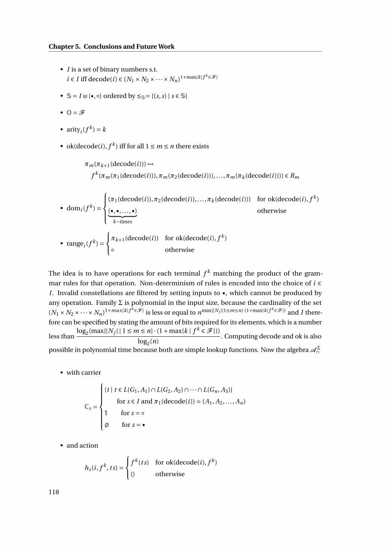
Chapter 5. Conclusions and Future Work
• I is a set of binary numbers s.t.
i ∈ I iff decode(i ) ∈ (N1 ×N2 ×·· ·×Nn)1+max{k| f k∈F }
• S= I ⊎ {•,◦} ordered by ≤S= {(s, s) | s ∈S}
• O=F
• arityi ( f k ) = k
• ok(decode(i ), f k ) iff for all 1 ≤ m ≤ n there exists
πm(πk+1(decode(i ))) ↦→f k (πm(π1(decode(i ))),πm(π2(decode(i ))), . . . ,πm(πk (decode(i )))) ∈ Rm
• domi ( f k ) =
⎧⎪⎪⎨⎪⎪⎩(π1(decode(i )),π2(decode(i )), . . . ,πk (decode(i ))) for ok(decode(i ), f k )
(•,•, . . . ,•)⏞ ⏟⏟ ⏞k−times
otherwise
• rangei ( f k ) =⎧⎨⎩πk+1(decode(i )) for ok(decode(i ), f k )
◦ otherwise
The idea is to have operations for each terminal f k matching the product of the gram-
mar rules for that operation. Non-determinism of rules is encoded into the choice of i ∈I . Invalid constellations are filtered by setting inputs to •, which cannot be produced by
any operation. Family Σ is polynomial in the input size, because the cardinality of the set
(N1 ×N2 ×·· ·×Nn)1+max{k| f k∈F } is less or equal to nmax{|N j ||1≤m≤n}·(1+max{k| f k∈F }) and I there-
fore can be specified by stating the amount of bits required for its elements, which is a number
less thanlog2(max{|N j | | 1 ≤ m ≤ n} · (1+max{k | f k ∈F }))
log2(n). Computing decode and ok is also
possible in polynomial time because both are simple lookup functions. Now the algebra A Σ∩
• with carrier
Cs =
⎧⎪⎪⎪⎪⎪⎪⎨⎪⎪⎪⎪⎪⎪⎩
{t | t ∈ L(G1, A1)∩L(G2, A2)∩·· ·∩L(Gn , A3)}
for s ∈ I and π1(decode(i )) = (A1, A2, . . . , An)
1 for s = ◦∅ for s = •
• and action
hs(i , f k , t s) =⎧⎨⎩ f k (t s) for ok(decode(i ), f k )
() otherwise
118

generates AlgGenA Σ
∩s =⋂
1≤i≤n L(Gi ) for sort s with decode(s) = (S1,S2, . . . ,Sn). Deciding empti-
ness of AlgGenA Σ
∩s therefore solves the intersection problem of Tree Grammars and sort-
emptiness is EXPTIME-hard.
From a practical standpoint, the conjecture above raises the question of when scalability limits
of the approach will be reached. When they are reached at some point, a possible idea is to
try to overcome the compositionaly limitations of machine learning discussed in Section 1.1.
Insights from the CoqHammer project [44] show, that a major problem for constructing proofs
(or programs) out of large knowledge bases is preimse selection. In Combinatory Logic, this
could be addressed by giving more structure to the context Γ. It would be interesting to
investigate adding a rule such as
CanReach(Γ1,Γ2) PlausibleFor(Γ2, A) Γ2 ⊢ M : AΓ1 ⊢ M : A
where predicate CanReach(Γ1,Γ2) is a user-defined or machine-learned relation on contexts,
and PlausibleFor(Γ2, A) is a machine-learned predicate on contexts and types, that limits the
search space.
A current drawback of the completely language-agnostic approach is that sometimes irrelevant
terms can be generated. An example is id(. . . id(id(x)) . . . ) where x is the only interesting
inhabitant. Some of the equational methods used in SyGus might be applicable for filtering
these irrelevant results. Most authors in literature equip algebraic signatures with equations
and so it seems obvious that the work presented here should be extended in this direction.
Finally many more practical applications of language-agnostic synthesis remain to be found.
The promising successes regarding synthesis problems in software product lines and the initial
steps toward more usability, even by non-experts, should be a start, rather than an end of a
journey.
119

Chapter 5. Conclusions and Future Work
120

Appendix A
Appendix
Section/Statement File Name in Coq
1 2.3/Lemma 1 Types.v Semantics_functional2 2.3/Lemma 2 Types.v subtype_total3 2.3/Lemma 3.1 Types.v bcd_cat_bigcap_f4 2.3/Lemma 3.2 Types.v bigcap_omega5 2.3/Lemma 3.3 Types.v bigcap_cast__ctor6 2.3/Lemma 3.4 Types.v bigcap_cast__Arr7 2.3/Lemma 3.5 Types.v bigcap_cast__Prod8 2.3/Lemma 3.6 Types.v bcd__Arr9 2.3/Lemma 3.7 Types.v bcd__ProdDist
10 2.3/Lemma 3.8 Cover.v bcd_subset_f11 2.3/Lemma 4 Types.v subty__sound12 2.3/Lemma 5.1 Types.v subty__omega13 2.3/Lemma 5.2 Types.v check__tgt__subseq14 2.3/Lemma 5.3 Types.v Omega__tgts15 2.3/Lemma 5.4 Types.v Omega__subty16 2.3/Lemma 5.5 Types.v weaken_check_tgt17 2.3/Lemma 5.6 Types.v subty__weaken18 2.3/Lemma 5.7 Types.v subty__cat19 2.3/Lemma 5.8 Types.v subty__CtorTrans20 2.3/Lemma 5.9 Types.v omegaDoneTgt21 2.3/Lemma 5.10 Types.v subty__Refl22 2.3/Lemma 5.11 Types.v split_tgts_for_srcs_gte23 2.3/Lemma 5.12 FCL.v tgt_for_srcs_gte_cat24 2.3/Lemma 5.13 Types.v subty__left, subty__right25 2.3/Lemma 5.14 Types.v can_cast_trans__Ctor,
can_cast_trans__Prod
121

Appendix A. Appendix
Section/Statement File Name in Coq
26 2.3/Lemma 5.15 Types.v subty__Trans27 2.3/Lemma 5.16 Types.v subty__CtorDist28 2.3/Lemma 5.17 Types.v subty__Idem29 2.3/Lemma 6 Types.v subty_complete30 2.3/Theorem 1 Types.v subtype_machine_correct,
subtypeMachineP31 2.3/Lemma 7 Types.v Domain_size32 2.3/Lemma 8 Types.v primeComponentPrime33 2.3/Lemma 9.1 Types.v addAndFilterLeq__A34 2.3/Lemma 9.2 Types.v addAndFilterLeq__DeltaA35 2.3/Lemma 9.3 Types.v addAndFilter_has_le_weaken36 2.3/Lemma 9.4 Types.v addAndFilter_in37 2.3/Lemma 9.5 Types.v bigcap_has_le38 2.3/Lemma 9.6 Types.v addAndFilter_monotonic39 2.3/Lemma 9.7 FCL.v all_addAndFilter40 2.3/Lemma 9.8 Types.v primeFactors_rec_prime41 2.3/Lemma 9.9 Types.v primeFactors_monotonic42 2.3/Lemma 9.10 Types.v primeFactors_rec_leq43 2.3/Lemma 9.11 Types.v addAndFilterGeq__Delta44 2.3/Lemma 9.12 Types.v bcd_all_ge45 2.3/Lemma 9.13 Types.v addAndFilterGeq46 2.3/Lemma 9.14 Types.v primeFactors_rec_geq47 2.3/Lemma 9.15 Types.v addAndFilter_nosubdup48 2.3/Lemma 9.16 Types.v primeFactors_nosubdup49 2.3/Lemma 9.17 Types.v primeFactors__notOmega50 2.3/Lemma 9.18 Types.v desubdup_nosubdupb51 2.3/Lemma 9.19 Types.v desubdup_all52 2.3/Lemma 9.20 Types.v desubdup_leq53 2.3/Lemma 9.21 Types.v desubdup_geq54 2.3/Lemma 9.22 Types.v addAndFilter_size55 2.3/Lemma 9.23 Types.v desubdup_size56 2.3/Lemma 9.24 Types.v desubdup_notOmega57 2.3/Lemma 9.25 Types.v bcd_prime_ge_all58 2.3/Lemma 9.26 Types.v prime_filter_le59 2.3/Lemma 9.27 Types.v nosubdup_unique60 2.3/Lemma 9.28 Types.v nosubdup_prime_injective61 2.3/Lemma 9.29 Types.v nosubdup_prime_bijective62 2.3/Lemma 9.30 Types.v nosubdup_weaken63 2.3/Lemma 9.31 Types.v bcd_prime_strengthen64 2.3/Lemma 9.32 Types.v nosubdup_everywhere65 2.3/Lemma 9.33 Types.v nosubdup_prime_perm
122

Section/Statement File Name in Coq
66 2.3/Lemma 9.34 Types.v PermUpToSubtyping_size67 2.3/Theorem 2.1 Types.v primeFactors_leq68 2.3/Theorem 2.2 Types.v primeFactors_geq69 2.3/Theorem 2.3 Types.v primeFactors_prime70 2.3/Theorem 2.4 Types.v primeFactors_minimal71 2.4/Lemma 10.1 FCL.v FCL_ind
(automatically generated by Coq)
72 2.4/Lemma 10.2 FCL.v FCL_Var_le73 2.4/Lemma 10.3 FCL.v FCL_MP_inv74 2.4/Lemma 10.4 FCL.v FCL_normalized_ind75 2.4/Lemma 11 FCL.v FCL_II, FCL_Omega76 2.4/Lemma 12 FCL.v FCL_weaken77 2.4/Lemma 13.1 Cover.v mkArrow_arrow78 2.4/Lemma 13.2 Cover.v mkArrow_rcons79 2.4/Lemma 13.3 Cover.v mkArrow_arity80 2.4/Lemma 13.4 Cover.v mkArrow_tgt_le81 2.4/Lemma 13.5 Cover.v omega_mkArrow_tgt82 2.4/Lemma 13.6 Cover.v mkArrow_prime83 2.4/Lemma 13.7 Cover.v mkArrow_dist84 2.4/Lemma 13.8 Cover.v mkArrow_srcs_ge85 2.4/Lemma 14.1 Algebra.v revApply_rcons86 2.4/Lemma 14.2 Algebra.v revApply_nil87 2.4/Lemma 14.3 FCL.v revApply_unapply88 2.4/Lemma 14.4 FCL.v unapply_revApply89 2.4/Lemma 15.1 FCL.v FCL__App90 2.4/Lemma 15.2 FCL.v FCL__invApp91 2.4/Lemma 16.1 FCL.v minimalArrowType_le92 2.4/Lemma 16.2 FCL.v minimalType_sound93 2.4/Lemma 16.3 FCL.v minimalArrowType_minimal94 2.4/Lemma 16.4 FCL.v minimalType_minimal95 2.4/Theorem 3 FCL.v fclP96 2.4.2/Lemma 17.1 FCL.v inPartition1_bigcap97 2.4.2/Lemma 17.2 FCL.v inPartition2_bigcap98 2.4.2/Lemma 17.3 FCL.v inPartition1_minimalType99 2.4.2/Lemma 17.4 FCL.v inPartition2_minimalType
100 2.4.2/Lemma 17.5 FCL.v minimalType_partitioned101 2.4.2/Theorem 4 FCL.v FCL__split102 2.4.2/Lemma 18.1 FCL.v bigcap_hom103 2.4.2/Lemma 18.2 FCL.v hom_arrow_cast104 2.4.2/Lemma 18.3 FCL.v minimalType_hom105 2.4.2/Lemma 18.4 FCL.v FCL__hom
123

Appendix A. Appendix
Section/Statement File Name in Coq
106 2.4.2/Lemma 19.1 FCL.v lift_arrow_hom107 2.4.2/Lemma 19.2 FCL.v lift_inter_hom108 2.4.2/Lemma 19.3 FCL.v lift_arrow_preimage109 2.4.2/Lemma 19.4 FCL.v lift_omega_hom110 2.4.2/Lemma 19.5 FCL.v unlift_lift111 2.4.2/Lemma 19.6 FCL.v lift_map_bigcap112 2.4.2/Lemma 19.7 FCL.v lift_cast_ctor113 2.4.2/Lemma 19.8 FCL.v isOmega_lift114 2.4.2/Lemma 19.9 FCL.v lift_cast_arr115 2.4.2/Lemma 19.10 FCL.v lift_cast_prod116 2.4.2/Lemma 19.11 FCL.v lift_cast_inter_prod117 2.4.2/Lemma 19.12 FCL.v lift_subtype_hom118 2.4.2/Lemma 19.13 FCL.v inPartition_lift1,
inPartition_lift2119 2.4.2/Lemma 19.14 FCL.v dist_arr_inPartition120 2.4.2/Lemma 19.15 FCL.v dist_inter_inPartition121 2.4.2/Lemma 19.16 FCL.v omega_inPartition122 2.4.2/Lemma 19.17 FCL.v inPartition_cast_ctor123 2.4.2/Lemma 19.18 FCL.v st_omega_inPartition124 2.4.2/Lemma 19.19 FCL.v primeComponents_inPartition125 2.4.2/Lemma 19.20 FCL.v st_irrel_check_inPartition126 2.4.2/Theorem 5 FCL.v canonicalCoproductLifted127 2.5.1/Lemma 20.1 Cover.v coverMachineFunctional_step128 2.5.1/Lemma 20.2 Cover.v coverMachineFunctional129 2.5.1/Lemma 21.1 Cover.v stepSize130 2.5.1/Lemma 21.2 Cover.v maxSteps131 2.5.1/Lemma 21.3 Cover.v Domain_total132 2.5.1/Lemma 22.1 Cover.v step_programStack133 2.5.1/Lemma 22.2 Cover.v step_stateMonotonic134 2.5.1/Lemma 22.3 Cover.v steps_stateMonotonic135 2.5.1/Lemma 23.1 Cover.v filterMergeMultiArrows_cat136 2.5.1/Lemma 23.2 Cover.v filterMergeMultiArrows_subseq137 2.5.1/Lemma 23.3 Cover.v filterMergeMultiArrows_map_cons138 2.5.1/Lemma 23.4 Cover.v step_mergeComponents139 2.5.1/Lemma 23.5 Cover.v step_sound140 2.5.1/Lemma 23.6 Cover.v splitsTail141 2.5.1/Lemma 23.7 Cover.v step_mergeComponents_in142 2.5.1/Lemma 23.8 Cover.v sound_reverse143 2.5.1/Lemma 23.9 Cover.v semantics_mergeComponents144 2.5.1/Lemma 24.1 Cover.v partitionCover_subset145 2.5.1/Lemma 24.2 Cover.v partitionCover_notSubset
124

Section/Statement File Name in Coq
146 2.5.1/Lemma 24.3 Cover.v partitionCover_subseq1147 2.5.1/Lemma 24.4 Cover.v partitionCover_subseq2148 2.5.1/Lemma 24.5 Cover.v instructions_covered_step149 2.5.1/Lemma 24.6 Cover.v not_omega_instruction_step150 2.5.1/Lemma 24.7 Cover.v arity_equal_step151 2.5.1/Lemma 24.8 Cover.v mergeMultiArrows_arity152 2.5.1/Lemma 24.9 Cover.v mergeMultiArrow_tgt_le153 2.5.1/Lemma 24.10 Cover.v mergeMultiArrow_tgt_ge154 2.5.1/Lemma 24.11 Cover.v mergeMultiArrow_srcs_le155 2.5.1/Lemma 24.12 Cover.v mergeMultiArrow_srcs_ge156 2.5.1/Lemma 24.13 Cover.v mergeMultiArrows_tgt_le157 2.5.1/Lemma 24.14 Cover.v mergeMultiArrows_tgt_ge158 2.5.1/Lemma 24.15 Cover.v mergeMultiArrows_srcs_le159 2.5.1/Lemma 24.16 Cover.v mergeMultiArrows_srcs_ge160 2.5.1/Lemma 24.17 Cover.v toCover_prime_step161 2.5.1/Lemma 24.18 Cover.v partitionCover_prime162 2.5.1/Lemma 24.19 Cover.v filterMergedArrows_in_cons163 2.5.1/Lemma 24.20 Cover.v covered_head_tgt164 2.5.1/Lemma 24.21 Cover.v partitionCover_drop1165 2.5.1/Lemma 24.22 Cover.v partitionCover_drop2166 2.5.1/Lemma 24.23 Cover.v mergeMultiArrows_cons_arity167 2.5.1/Lemma 24.24 Cover.v partitionCover_complete168 2.5.1/Lemma 24.25 Cover.v partition_cover_both169 2.5.1/Lemma 24.26 Cover.v complete_partitionCover170 2.5.1/Lemma 24.27 Cover.v currentResultNotDone_step171 2.5.1/Lemma 24.28 Cover.v notDone_incomplete172 2.5.1/Lemma 24.29 Cover.v filterMergeMultiArrows_map_cons2173 2.5.1/Lemma 24.30 Cover.v mergeMultiArrow_srcs_monotonic174 2.5.1/Lemma 24.31 Cover.v cap_dcap175 2.5.1/Lemma 24.32 Cover.v dcap_cap176 2.5.1/Lemma 24.33 Cover.v mergeMultiArrow_srcs_map_zip177 2.5.1/Lemma 24.34 Cover.v impossible_notSubtype178 2.5.1/Lemma 24.35 Cover.v complete_reverse179 2.5.1/Lemma 24.36 Cover.v steps_complete180 2.5.1/Lemma 25.1 Cover.v step_tgt_sound181 2.5.1/Lemma 25.2 Cover.v step_tgt_sound_reverse182 2.5.1/Lemma 25.3 Cover.v steps_tgt_sound183 2.5.1/Lemma 26.1 Cover.v arity_increasing_cat184 2.5.1/Lemma 26.2 Cover.v splitRec_arity185 2.5.1/Lemma 26.3 Cover.v splitTy_arity186 2.5.1/Lemma 26.4 Cover.v arity_increasing_arity_equal
125

Appendix A. Appendix
Section/Statement File Name in Coq
187 2.5.1/Lemma 26.5 Cover.v splitRec_monotonic188 2.5.1/Lemma 26.6 Cover.v splitRec_context_size_eq189 2.5.1/Lemma 26.7 Cover.v splitRec_context_monotonic190 2.5.1/Lemma 26.8 Cover.v splitRec_split_context191 2.5.1/Lemma 26.9 Cover.v splitRec_sound192 2.5.1/Lemma 26.10 Cover.v splitTy_sound193 2.5.1/Lemma 26.11 Cover.v merge_assoc194 2.5.1/Lemma 26.12 Cover.v merges0195 2.5.1/Lemma 26.13 Cover.v merge0s196 2.5.1/Lemma 26.14 Cover.v splitRec_merge197 2.5.1/Lemma 26.15 Cover.v map_merge198 2.5.1/Lemma 26.16 Cover.v splitRec_rcat199 2.5.1/Lemma 26.17 Cover.v splitTy_slow_splitTy200 2.5.1/Lemma 26.18 Cover.v splitTy_slow_omega201 2.5.1/Lemma 26.19 Cover.v nth_merge202 2.5.1/Lemma 26.20 Cover.v splitTy_slow_inter_subseq2203 2.5.1/Lemma 26.21 Cover.v splitTy_complete_ctor204 2.5.1/Lemma 26.22 Cover.v splitTy_complete_prod205 2.5.1/Lemma 26.23 Cover.v splitTy_complete_omega206 2.5.1/Lemma 26.24 Cover.v splitTy_complete_alternative207 2.5.1/Lemma 26.25 Cover.v splitTy_complete208 2.5.1/Lemma 27.1 Cover.v splitTy_instructionsCovered209 2.5.1/Lemma 27.2 Cover.v coverMachine_splitTy_complete210 2.5.1/Lemma 27.3 Cover.v bcd_multiArrow_Dist211 2.5.1/Lemma 27.4 Cover.v coverMachine_splitTy_sound212 2.5.1/Lemma 27.5 Cover.v coverMachine_splitTy_tgt_sound213 2.5.1/Lemma 28.1 Cover.v reduction_subseq214 2.5.1/Lemma 28.2 Cover.v soundnessPreserving215 2.5.1/Lemma 28.3 Cover.v tgt_soundnessPreserving216 2.5.1/Lemma 28.4 Cover.v completenessPreserving217 2.5.2/Lemma 29.1 FCL.v FCL_sound_sound218 2.5.2/Lemma 29.2 FCL.v dropTargets_suffix219 2.5.2/Lemma 29.3 FCL.v suffix_word220 2.5.2/Lemma 29.4 FCL.v suffix_sound221 2.5.2/Lemma 29.5 FCL.v cat_sound222 2.5.2/Lemma 29.6 FCL.v commitMultiArrow_sound223 2.5.2/Lemma 29.7 FCL.v commitUpdates_sound224 2.5.2/Lemma 29.8 FCL.v accumulateCovers_sound225 2.5.2/Lemma 29.9 FCL.v foldl_accumulateCovers_sound226 2.5.2/Lemma 29.10 FCL.v inhabit_cover_sound227 2.5.2/Lemma 29.11 FCL.v OmegaRules_sound
126

Section/Statement File Name in Coq
228 2.5.2/Lemma 29.12 FCL.v inhabitation_step_sound229 2.5.2/Lemma 29.13 FCL.v inhabit_multistep_sound230 2.5.2/Lemma 30 FCL.v InhabitationSemantics_functional_step231 2.5.2/Lemma 31.1 FCL.v grammarTypes_src_mem232 2.5.2/Lemma 31.2 FCL.v grammarTypes_tgt_mem233 2.5.2/Lemma 31.3 FCL.v commitMultiArrow_parameterTypes_subset234 2.5.2/Lemma 31.4 FCL.v commitUpdates_parameterTypes_subset235 2.5.2/Lemma 31.5 FCL.v accumulateCovers_parameterTypes_subset236 2.5.2/Lemma 31.6 FCL.v maxParameterTypes_initialTarget237 2.5.2/Lemma 31.7 FCL.v foldl_accumulateCovers_
parameterTypes_subset238 2.5.2/Lemma 31.8 FCL.v inhabit_cover_parameterTypes_subset239 2.5.2/Lemma 31.9 FCL.v OmegaRules_params240 2.5.2/Lemma 31.10 FCL.v OmegaRules_subset241 2.5.2/Lemma 31.11 FCL.v inhabitation_step_subset242 2.5.2/Lemma 31.12 FCL.v inhabit_step_rel_wf243 2.5.2/Lemma 31.13 FCL.v inhabit_step_rel_cons244 2.5.2/Lemma 31.14 FCL.v dropTargets_size245 2.5.2/Lemma 31.15 FCL.v commitUpdates_nil_eq246 2.5.2/Lemma 31.16 FCL.v reduceMultiArrows_nil247 2.5.2/Lemma 31.17 FCL.v accumulateCovers_failed_targets_eq248 2.5.2/Lemma 31.18 FCL.v accumulateCovers_failed_rev249 2.5.2/Lemma 31.19 FCL.v foldl_accumulateCovers_failed_rev250 2.5.2/Lemma 31.20 FCL.v foldl_accumulateCovers_
failed_targets_eq251 2.5.2/Lemma 31.21 FCL.v inhabit_cover_failed_targets_eq252 2.5.2/Lemma 31.22 FCL.v computeFailExisting_notFound253 2.5.2/Lemma 31.23 FCL.v inhabitation_step_sizes254 2.5.2/Lemma 31.24 FCL.v domain_start255 2.5.2/Lemma 32.1 FCL.v FailSound_cat256 2.5.2/Lemma 32.2 FCL.v cat_FailSound257 2.5.2/Lemma 32.3 FCL.v computeFailExisting_FailSound258 2.5.2/Lemma 32.4 FCL.v accumulateCovers_FailSound259 2.5.2/Lemma 32.5 FCL.v inhabit_cover_FailSound260 2.5.2/Lemma 32.6 FCL.v OmegaRules_FailSound261 2.5.2/Lemma 32.7 FCL.v inhabit_step_FailSound262 2.5.2/Lemma 32.8 FCL.v noTargetFailures_suffix263 2.5.2/Lemma 32.9 FCL.v inhabit_cover_noTargetFailures264 2.5.2/Lemma 32.10 FCL.v inhabitation_step_noTargetFailures265 2.5.2/Lemma 33.1 FCL.v cancel_group_flatten
127

Appendix A. Appendix
Section/Statement File Name in Coq
266 2.5.2/Lemma 33.2 FCL.v updateGroups0267 2.5.2/Lemma 33.3 FCL.v group_notComb268 2.5.2/Lemma 33.4 FCL.v group_comb269 2.5.2/Lemma 33.5 FCL.v dropTargets_notCombinator270 2.5.2/Lemma 33.6 FCL.v dropTargets_combinatorOrEmpty271 2.5.2/Lemma 33.7 FCL.v group_split272 2.5.2/Lemma 33.8 FCL.v FCL_complete_emptyTargets273 2.5.2/Lemma 33.9 FCL.v future_word_word274 2.5.2/Lemma 33.10 FCL.v future_word_weaken275 2.5.2/Lemma 33.11 FCL.v rule_absorbl276 2.5.2/Lemma 33.12 FCL.v future_word_dropFailed277 2.5.2/Lemma 33.13 FCL.v computeFailExisting_failed_complete278 2.5.2/Lemma 33.14 FCL.v rule_absorbl_apply279 2.5.2/Lemma 33.15 FCL.v computeFailExisting_existing280 2.5.2/Lemma 33.16 FCL.v OmegaRules_future_word281 2.5.2/Lemma 33.17 FCL.v rule_MP282 2.5.2/Lemma 33.18 FCL.v FCL_Omega_complete283 2.5.2/Lemma 33.19 FCL.v accumulateCovers_cat284 2.5.2/Lemma 33.20 FCL.v inhabit_cover_flatten285 2.5.2/Lemma 33.21 FCL.v inhabit_cover_empty286 2.5.2/Lemma 33.22 FCL.v commitMultiArrow_cons287 2.5.2/Lemma 33.23 FCL.v commitUpdates_flatten288 2.5.2/Lemma 33.24 FCL.v commitMultiArrow_size289 2.5.2/Lemma 33.25 FCL.v commitMultiArrow_nth290 2.5.2/Lemma 33.26 FCL.v commitMultiArrows_combinatorOrEmpty291 2.5.2/Lemma 33.27 FCL.v nextTargets_combinatorOrEmpty292 2.5.2/Lemma 33.28 FCL.v group_commitMultiArrow293 2.5.2/Lemma 33.29 FCL.v future_word_weaken_inhabapply294 2.5.2/Lemma 33.30 FCL.v commitMultiArrow_parameters295 2.5.2/Lemma 33.31 FCL.v future_word_weaken_targets1296 2.5.2/Lemma 33.32 FCL.v future_word_weaken_targets2297 2.5.2/Lemma 33.33 FCL.v future_word_covers298 2.5.2/Lemma 33.34 FCL.v rule_absorbl_apply_covers299 2.5.2/Lemma 33.35 FCL.v prefix_target_groups300 2.5.2/Lemma 33.36 FCL.v nil_reduceMultiArrows301 2.5.2/Lemma 33.37 FCL.v empty_inhabit_cover302 2.5.2/Lemma 33.38 FCL.v cover_targets303 2.5.2/Lemma 33.39 FCL.v inhabit_cover_complete304 2.5.2/Lemma 33.40 FCL.v inhabit_step_complete305 2.5.2/Lemma 33.41 FCL.v inhabit_multistep_complete306 2.5.2/Theorem 6.1 FCL.v inhabit_sound
128

Section/Statement File Name in Coq
307 2.5.2/Theorem 6.2 FCL.v inhabit_complete308 2.6.2/Lemma 34.1 TwoCounter.v sound_Sigma__Aut309 2.6.2/Lemma 34.2 TwoCounter.v sound310 2.6.2/Lemma 34.3 TwoCounter.v complete311 2.6.3/Lemma 35.1 DependentFixpoint.v Fix_F_inv312 2.6.3/Lemma 35.2 DependentFixpoint.v isFix_unique313 2.6/Lemma 36.1 Algebra.v canonical_morphism_commutes314 2.6/Lemma 36.2 Algebra.v canonical_morphism_alg_morphism315 2.6/Lemma 36.3 Algebra.v canonical_morphism_unique316 2.6/Lemma 36.4 Algebra.v canonical_morphism_sound317 2.6/Lemma 36.5 Algebra.v canonical_morphism_complete318 2.6/Lemma 37.1 Algebra.v embed_unembed319 2.6/Lemma 37.2 Algebra.v embed_le320 2.6/Lemma 37.3 Algebra.v proofAction_FCL321 2.6/Lemma 37.4 Algebra.v unapplyNotIndex322 2.6/Lemma 37.5 Algebra.v arrow_le323 2.6/Lemma 37.6 Algebra.v indexType_sound324 2.6/Lemma 37.7 Algebra.v unapplyIsIndex325 2.6/Lemma 37.8 Algebra.v termCoAction_size326 2.6/Lemma 37.9 Algebra.v proofCoAction__FCL327 2.6/Lemma 37.10 Algebra.v range_coAction328 2.6/Lemma 38.1 Algebra.v Term_unapply_ind329 2.6/Lemma 38.2 Algebra.v IsChild_wf330 2.6/Lemma 38.3 Algebra.v dec_coAction__FCL331 2.6/Lemma 38.4 Algebra.v cancel_action_coAction__FCL332 2.6/Lemma 38.5 Algebra.v cancel_coAction__FCL_action333 2.6/Theorem 7.1 Algebra.v unique334 2.6/Theorem 7.2 Algebra.v sound335 2.6/Theorem 7.3 Algebra.v complete
Table A.1: Statements and where to find their Coq formalization in [15]
129

Appendix A. Appendix
130
Bibliography
[1] J. Adámek and S. Milius. Introduction to Category Theory, Algebras and Coalgebra, 2010.
URL https://www.tu-braunschweig.de/Medien-DB/iti/survey_full.pdf. Lecture Notes
of the European Summer School on Logic, Language and Information (ESSLLI 2010).
[2] R. Alur, R. Bodík, G. Juniwal, M. M. K. Martin, M. Raghothaman, S. A. Seshia, R. Singh,
A. Solar-Lezama, E. Torlak, and A. Udupa. Syntax-guided synthesis. In Formal Methods
in Computer-Aided Design, FMCAD 2013, Portland, OR, USA, October 20-23, 2013, pages
1–8, 2013. URL http://ieeexplore.ieee.org/document/6679385/.
[3] R. Alur, D. Fisman, R. Singh, A. Solar-Lezama, et al. Syntax Guided Synthesis (SyGus)
Competitions, 2014–2019. URL http://sygus.seas.upenn.edu/.
[4] Apache Foundation. Apache License Version 2.0, 2004. URL http://www.apache.org/
licenses/LICENSE-2.0.
[5] S. Apel, C. Kästner, and C. Lengauer. Language-Independent and Automated Software
Composition: The FeatureHouse Experience. IEEE Trans. Software Eng., 39(1):63–79,
2013. doi: 10.1109/TSE.2011.120. URL https://doi.org/10.1109/TSE.2011.120.
[6] Association for Computing Machinery (ACM) Special Interest Group on programming
languages (SIGPLAN). Synthesis Track at Principles of Programming Languages (POPL),
2013–2019. URL http://www.sigplan.org/Conferences/POPL/.
[7] L. Augustsson. Djinn, a theorem prover in Haskell, for Haskell, 2005. URL http://hackage.
haskell.org/package/djinn.
[8] H. Barendregt, M. Coppo, and M. Dezani-Ciancaglini. A Filter Lambda Model and the
Completeness of Type Assignment. J. Symb. Log., 48(4):931–940, 1983. doi: 10.2307/
2273659. URL https://doi.org/10.2307/2273659.
[9] H. P. Barendregt, W. Dekkers, and R. Statman. Lambda Calculus with Types.
Perspectives in logic. Cambridge University Press, 2013. ISBN 978-0-521-
76614-2. URL http://www.cambridge.org/de/academic/subjects/mathematics/
logic-categories-and-sets/lambda-calculus-types.
[10] B. Barras. Sets in Coq, Coq in Sets. J. Formalized Reasoning, 3(1):29–48, 2010. doi:
10.6092/issn.1972-5787/1695. URL https://doi.org/10.6092/issn.1972-5787/1695.
131

Bibliography
[11] M. Ben-Soula, J. Hesse, et al. Maven Central - Repository for jar-file based dependencies,
2019. URL https://search.maven.org/.
[12] C.-B. Ben-Yelles. Type assignment in the lambda-calculus: Syntax and semantics. PhD
thesis, University College of Swansea, 1979.
[13] M. Benke, A. Schubert, and D. Walukiewicz-Chrzaszcz. Synthesis of Functional Programs
with Help of First-Order Intuitionistic Logic. In 1st International Conference on Formal
Structures for Computation and Deduction, FSCD 2016, June 22-26, 2016, Porto, Portugal,
pages 12:1–12:16, 2016. doi: 10.4230/LIPIcs.FSCD.2016.12. URL https://doi.org/10.4230/
LIPIcs.FSCD.2016.12.
[14] J. Bessai. Synthesizing Dependency Injection Configurations for the Spring Framework,
2014. Master’s Thesis, Technical University of Dortmund.
[15] J. Bessai. cls-coq: The Coq Formalization of the (CL)S Framework, 2019. URL https:
//doi.org/10.5281/zenodo.3243398.
[16] J. Bessai. Usage example of cls-scala, 2019. URL https://github.com/combinators/
nosurrender.
[17] J. Bessai. cls-coq: Old version of the Coq Formalization of the (CL)S Framework, 2019.
URL https://doi.org/10.5281/zenodo.3243395.
[18] J. Bessai and A. Vasileva. User Support for the Combinator Logic Synthesizer Frame-
work. In Proceedings 4th Workshop on Formal Integrated Development Environ-
ment, F-IDE@FLoC 2018, Oxford, England, 14 July 2018., pages 16–25, 2018. doi:
10.4204/EPTCS.284.2. URL https://doi.org/10.4204/EPTCS.284.2.
[19] J. Bessai, B. Düdder, A. Dudenhefer, and M. Martens. Delegation-based Mixin Composi-
tion Synthesis. Proceedings of Intersection Types and Related Systems (ITRS’14), Lecture
Notes in Computer Science. Springer, 2014a.(Cited on pages 14 and 115), 2014.
[20] J. Bessai, A. Dudenhefner, B. Düdder, M. Martens, and J. Rehof. Combinatory Logic
Synthesizer. In Leveraging Applications of Formal Methods, Verification and Validation.
Technologies for Mastering Change - 6th International Symposium, ISoLA 2014, Imperial,
Corfu, Greece, October 8-11, 2014, Proceedings, Part I, pages 26–40, 2014. doi: 10.1007/
978-3-662-45234-9\_3. URL https://doi.org/10.1007/978-3-662-45234-9_3.
[21] J. Bessai, B. Düdder, G. T. Heineman, and J. Rehof. Combinatory Synthesis of Classes
Using Feature Grammars. In Formal Aspects of Component Software - 12th International
Conference, FACS 2015, Niterói, Brazil, October 14-16, 2015, Revised Selected Papers,
pages 123–140, 2015. doi: 10.1007/978-3-319-28934-2\_7. URL https://doi.org/10.1007/
978-3-319-28934-2_7.
[22] J. Bessai, A. Dudenhefner, B. Düdder, T. Chen, U. de’Liguoro, and J. Rehof. Mixin
Composition Synthesis Based on Intersection Types. In 13th International Conference
132

Bibliography
on Typed Lambda Calculi and Applications, TLCA 2015, July 1-3, 2015, Warsaw, Poland,
pages 76–91, 2015. doi: 10.4230/LIPIcs.TLCA.2015.76. URL https://doi.org/10.4230/
LIPIcs.TLCA.2015.76.
[23] J. Bessai, A. Dudenhefner, B. Düdder, M. Martens, and J. Rehof. Combinatory Process
Synthesis. In Leveraging Applications of Formal Methods, Verification and Validation:
Foundational Techniques - 7th International Symposium, ISoLA 2016, Imperial, Corfu,
Greece, October 10-14, 2016, Proceedings, Part I, pages 266–281, 2016. doi: 10.1007/
978-3-319-47166-2\_19. URL https://doi.org/10.1007/978-3-319-47166-2_19.
[24] J. Bessai, A. Dudenhefner, B. Düdder, and J. Rehof. Extracting a formally verified Subtyp-
ing Algorithm for Intersection Types from Ideals and Filters. Types, 2016.
[25] J. Bessai, T. Chen, A. Dudenhefner, B. Düdder, U. de’Liguoro, and J. Rehof. Mixin
Composition Synthesis based on Intersection Types. Logical Methods in Computer
Science, 14(1), 2018. doi: 10.23638/LMCS-14(1:18)2018. URL https://doi.org/10.23638/
LMCS-14(1:18)2018.
[26] J. Bessai, B. Düdder, G. T. Heineman, and J. Rehof. Towards Language-independent
Code Synthesis, 2018. URL https://popl18.sigplan.org/details/PEPM-2018/12/
Towards-Language-independent-Code-Synthesis-Poster-Demo-Talk-. Poster and Talk.
[27] J. Bessai, B. Düdder, G. T. Heineman, et al. (CL)S Ecosystem, 2019. URL https://www.
combinators.org.
[28] J. Bessai, J. Rehof, and B. Düdder. Fast Verified BCD Subtyping. In T. Margaria, S. Graf,
and K. G. Larsen, editors, Models, Mindsets, Meta: The What, the How, and the Why Not?,
volume 11200 of LNCS. Springer, 2019. To appear.
[29] J. Bessai, A. Vasileva, and M. Roidl. Laser Visualization User Support for a cls-scala
Use-Case, 2019. URL https://github.com/combinators/labyrinth.
[30] X. Bi, B. C. d. S. Oliveira, and T. Schrijvers. The Essence of Nested Composition. In 32nd
European Conference on Object-Oriented Programming, ECOOP 2018, July 16-21, 2018,
Amsterdam, The Netherlands, pages 22:1–22:33, 2018. URL https://doi.org/10.4230/
LIPIcs.ECOOP.2018.22.
[31] R. Bodík, S. Gulwani, and E. Yahav. Software Synthesis (Dagstuhl Seminar 12152).
Dagstuhl Reports, 2(4):21–38, 2012. doi: 10.4230/DagRep.2.4.21. URL https://doi.org/
10.4230/DagRep.2.4.21.
[32] S. Böhme and T. Nipkow. Sledgehammer: Judgement Day. In Automated Reasoning, 5th
International Joint Conference, IJCAR 2010, Edinburgh, UK, July 16-19, 2010. Proceedings,
pages 107–121, 2010. doi: 10.1007/978-3-642-14203-1\_9. URL https://doi.org/10.1007/
978-3-642-14203-1_9.
[33] G. Bort et al. Play Web Framework, 2019. URL https://www.playframework.com/.
133

Bibliography
[34] B. Brayton et al. International Workshop on Logic and Synthesis, 1987–2019. URL
http://www.iwls.org.
[35] S. Broda and L. Damas. Counting a Type’s (Principal) Inhabitants. Fundam. Inform., 45
(1-2):33–51, 2001. URL http://content.iospress.com/articles/fundamenta-informaticae/
fi45-1-2-03.
[36] J. R. Büchi and L. H. Landweber. Solving Sequential Conditions by Finite-State Strategies.
Transactions of the American Mathematical Society, 138:295–311, 1969.
[37] W. E. Byrd and D. P. Friedman. From Variadic Functions to Variadic Relations – A
miniKaren Perspective. In Proceedings of the 2006 Scheme and Functional Programming
Workshop, University of Chicago Technical Report TR-2006-06, pages 105–117, 2006.
[38] W. E. Byrd, N. Amin, et al. Workshop on miniKaren, 2019. URL https://icfp19.sigplan.
org/home/minikanren-2019.
[39] W. E. Byrd et al. Homepage of the miniKaren Language, 2019. URL http://minikanren.
org/.
[40] F. Cardone and J. R. Hindley. Lambda-Calculus and Combinators in the 20th Century. In
Logic from Russell to Church, pages 723–817. Elsevier, 2009. doi: 10.1016/S1874-5857(09)
70018-4. URL https://doi.org/10.1016/S1874-5857(09)70018-4.
[41] J. Cockx, D. Devriese, and F. Piessens. Eliminating dependent pattern matching without
K. J. Funct. Program., 26:e16, 2016. doi: 10.1017/S0956796816000174. URL https:
//doi.org/10.1017/S0956796816000174.
[42] H. Comon, M. Dauchet, R. Gilleron, C. Löding, F. Jacquemard, D. Lugiez, S. Tison, and
M. Tommasi. Tree Automata Techniques and Applications. Online publication, October
2007. URL http://www.grappa.univ-lille3.fr/tata.
[43] M. Coppo, M. Dezani-Ciancaglini, and B. Venneri. Functional Characters of Solvable
Terms. Math. Log. Q., 27(2-6):45–58, 1981. doi: 10.1002/malq.19810270205. URL
https://doi.org/10.1002/malq.19810270205.
[44] L. Czajka, B. Ekici, and C. Kaliszyk. Concrete Semantics with Coq and CoqHam-
mer. In Intelligent Computer Mathematics - 11th International Conference, CICM
2018, Hagenberg, Austria, August 13-17, 2018, Proceedings, pages 53–59, 2018. doi:
10.1007/978-3-319-96812-4\_5. URL https://doi.org/10.1007/978-3-319-96812-4_5.
[45] F. M. Damm. Subtyping with Union Types, Intersection Types and Recursive Types. In
Theoretical Aspects of Computer Software, International Conference TACS ’94, Sendai,
Japan, April 19-22, 1994, Proceedings, pages 687–706, 1994. URL https://doi.org/10.
1007/3-540-57887-0_121.
[46] F. M. Damm. Subtyping with Union Types, Intersection Types and Recursive Types II. PhD
thesis, INRIA, 1994.
134

Bibliography
[47] R. Davies and F. Pfenning. A modal analysis of staged computation. J. ACM, 48(3):555–
604, 2001. doi: 10.1145/382780.382785. URL https://doi.org/10.1145/382780.382785.
[48] J. Denis. Entwurf und Implementierung eines synthesebasierten Ansatzes für die flexible
Ausführung von Geschäftsprozessen, 2018. Bachelor’s Thesis, Technical University of
Dortmund.
[49] M. Dezani-Ciancaglini and J. R. Hindley. Intersection Types for Combinatory Logic.
Theor. Comput. Sci., 100(2):303–324, 1992. doi: 10.1016/0304-3975(92)90306-Z. URL
https://doi.org/10.1016/0304-3975(92)90306-Z.
[50] M. Dezani-Ciancaglini and J. R. Hindley. Intersection Types for Combinatory Logic.
Theor. Comput. Sci., 100(2):303–324, 1992. doi: 10.1016/0304-3975(92)90306-Z. URL
https://doi.org/10.1016/0304-3975(92)90306-Z.
[51] C. Dion. I surrender. In A New Day Has Come. Columbia Records, 2002. Written by Louis
Biancaniello and Sam Watters.
[52] E. Doberkat. Special Topics in Mathematics for Computer Scientists - Sets, Categories,
Topologies and Measures. Springer, 2015. ISBN 978-3-319-22749-8. doi: 10.1007/
978-3-319-22750-4. URL https://doi.org/10.1007/978-3-319-22750-4.
[53] E.-E. Doberkat. Haskell: Eine Einführung für Objektorientierte. Walter de Gruyter, 2012.
ISBN 978-3486714173.
[54] Docker, Inc. The Docker Container Platform, 2019. URL www.docker.com.
[55] B. Düdder. Automatic Synthesis of Component & Connector Software Architectures with
Bounded Combinatory Logic. PhD thesis, Technical University Dortmund, Germany,
2014.
[56] B. Düdder, O. Garbe, M. Martens, J. Rehof, and P. Urzyczyn. Using Inhabitation in
Bounded Combinatory Logic with Intersection Types for Composition Synthesis. In
Proceedings Sixth Workshop on Intersection Types and Related Systems, ITRS 2012,
Dubrovnik, Croatia, 29th June 2012., pages 18–34, 2012. doi: 10.4204/EPTCS.121.2.
URL https://doi.org/10.4204/EPTCS.121.2.
[57] B. Düdder, M. Martens, J. Rehof, and P. Urzyczyn. Bounded Combinatory Logic. In
Computer Science Logic (CSL’12) - 26th International Workshop/21st Annual Conference
of the EACSL, CSL 2012, September 3-6, 2012, Fontainebleau, France, pages 243–258, 2012.
doi: 10.4230/LIPIcs.CSL.2012.243. URL https://doi.org/10.4230/LIPIcs.CSL.2012.243.
[58] B. Düdder, M. Martens, and J. Rehof. Intersection Type Matching with Subtyping. In
Typed Lambda Calculi and Applications, 11th International Conference, TLCA 2013,
Eindhoven, The Netherlands, June 26-28, 2013. Proceedings, pages 125–139, 2013. doi:
10.1007/978-3-642-38946-7\_11. URL https://doi.org/10.1007/978-3-642-38946-7_11.
135

Bibliography
[59] B. Düdder, M. Martens, and J. Rehof. Staged Composition Synthesis. In Programming
Languages and Systems - 23rd European Symposium on Programming, ESOP 2014,
Held as Part of the European Joint Conferences on Theory and Practice of Software,
ETAPS 2014, Grenoble, France, April 5-13, 2014, Proceedings, pages 67–86, 2014. doi:
10.1007/978-3-642-54833-8\_5. URL https://doi.org/10.1007/978-3-642-54833-8_5.
[60] B. Düdder, J. Rehof, and G. T. Heineman. Synthesizing type-safe compositions in
feature oriented software designs using staged composition. In Proceedings of the 19th
International Conference on Software Product Line, SPLC 2015, Nashville, TN, USA,
July 20-24, 2015, pages 398–401, 2015. doi: 10.1145/2791060.2793677. URL https:
//doi.org/10.1145/2791060.2793677.
[61] A. Dudenhefner. Algorithmic Aspects of Type-Based Program Synthesis. PhD thesis,
Technical University Dortmund, Germany, 2019.
[62] A. Dudenhefner. cls-fsharp, 2019. URL https://github.com/mrhaandi/cls-fsharp.
[63] A. Dudenhefner and J. Rehof. The Complexity of Principal Inhabitation. In 2nd Inter-
national Conference on Formal Structures for Computation and Deduction, FSCD 2017,
September 3-9, 2017, Oxford, UK, pages 15:1–15:14, 2017. doi: 10.4230/LIPIcs.FSCD.
2017.15. URL https://doi.org/10.4230/LIPIcs.FSCD.2017.15.
[64] A. Dudenhefner and J. Rehof. Typability in bounded dimension. In 32nd Annual
ACM/IEEE Symposium on Logic in Computer Science, LICS 2017, Reykjavik, Iceland, June
20-23, 2017, pages 1–12, 2017. doi: 10.1109/LICS.2017.8005127. URL https://doi.org/10.
1109/LICS.2017.8005127.
[65] A. Dudenhefner and J. Rehof. Intersection type calculi of bounded dimension. In
Proceedings of the 44th ACM SIGPLAN Symposium on Principles of Programming Lan-
guages, POPL 2017, Paris, France, January 18-20, 2017, pages 653–665, 2017. URL
http://dl.acm.org/citation.cfm?id=3009862.
[66] A. Dudenhefner and J. Rehof. Principality and approximation under dimensional bound.
PACMPL, 3(POPL):8:1–8:29, 2019. doi: 10.1145/3290321. URL https://doi.org/10.1145/
3290321.
[67] A. Dudenhefner, M. Martens, and J. Rehof. The Algebraic Intersection Type Unification
Problem. Logical Methods in Computer Science, 13(3), 2017. URL https://doi.org/10.
23638/LMCS-13(3:9)2017.
[68] J. Duregård, P. Jansson, and M. Wang. Feat: functional enumeration of algebraic types. In
Proceedings of the 5th ACM SIGPLAN Symposium on Haskell, Haskell 2012, Copenhagen,
Denmark, 13 September 2012, pages 61–72, 2012. doi: 10.1145/2364506.2364515. URL
https://doi.org/10.1145/2364506.2364515.
136
Bibliography
[69] R. Dyckhoff. Contraction-Free Sequent Calculi for intuitionistic Logic: a correction. J.
Symb. Log., 83(4):1680–1682, 2018. doi: 10.1017/jsl.2018.38. URL https://doi.org/10.
1017/jsl.2018.38.
[70] H. Ehrich. On the Theory of Specification, Implementation, and Parametrization of
Abstract Data Types. Journal of the ACM, 29(1):206–227, 1982. URL https://doi.org/10.
1145/322290.322303.
[71] H. Ehrig and B. Mahr. Fundamentals of Algebraic Specification 1: Equations und Initial
Semantics, volume 6 of EATCS Monographs on Theoretical Computer Science. Springer,
1985. ISBN 3-540-13718-1. URL https://doi.org/10.1007/978-3-642-69962-7.
[72] K. Ellis, E. Dechter, and J. B. Tenenbaum. Dimensionality Reduction via Program
Induction. In 2015 AAAI Spring Symposia, Stanford University, Palo Alto, California, USA,
March 22-25, 2015, 2015. URL http://www.aaai.org/ocs/index.php/SSS/SSS15/paper/
view/10284.
[73] Y. Feng, R. Martins, J. V. Geffen, I. Dillig, and S. Chaudhuri. Component-based synthesis
of table consolidation and transformation tasks from examples. In Proceedings of the
38th ACM SIGPLAN Conference on Programming Language Design and Implementation,
PLDI 2017, Barcelona, Spain, June 18-23, 2017, pages 422–436, 2017. doi: 10.1145/
3062341.3062351. URL https://doi.org/10.1145/3062341.3062351.
[74] Y. Feng, R. Martins, Y. Wang, I. Dillig, and T. W. Reps. Component-based synthesis for
complex APIs. In Proceedings of the 44th ACM SIGPLAN Symposium on Principles of
Programming Languages, POPL 2017, Paris, France, January 18-20, 2017, pages 599–612,
2017. URL http://dl.acm.org/citation.cfm?id=3009851.
[75] J. Filliâtre and S. Conchon. Type-safe modular hash-consing. In Proceedings of the ACM
Workshop on ML, 2006, Portland, Oregon, USA, September 16, 2006, pages 12–19, 2006.
doi: 10.1145/1159876.1159880. URL https://doi.org/10.1145/1159876.1159880.
[76] B. Finkbeiner, F. Klein, R. Piskac, and M. Santolucito. Synthesizing Functional Reactive
Programs. CoRR, abs/1905.09825, 2019. URL http://arxiv.org/abs/1905.09825.
[77] P. C. Fischer, A. R. Meyer, and A. L. Rosenberg. Counter Machines and Counter Lan-
guages. Mathematical Systems Theory, 2(3):265–283, 1968. doi: 10.1007/BF01694011.
URL https://doi.org/10.1007/BF01694011.
[78] J. Frankle, P. Osera, D. Walker, and S. Zdancewic. Example-directed synthesis: a type-
theoretic interpretation. In Proceedings of the 43rd Annual ACM SIGPLAN-SIGACT
Symposium on Principles of Programming Languages, POPL 2016, St. Petersburg, FL,
USA, January 20 - 22, 2016, pages 802–815, 2016. doi: 10.1145/2837614.2837629. URL
https://doi.org/10.1145/2837614.2837629.
[79] D. P. Friedman, W. E. Byrd, and O. Kiselyov. The Reasoned Schemer. MIT Press, 2005.
ISBN 978-0-262-56214-0.
137
Bibliography
[80] S. Fuchs et al. Travis CI - Continuous Integration Build Service, 2019. URL https:
//travis-ci.org/.
[81] E. Gamma, R. Helm, R. E. Johnson, and J. M. Vlissides. Design Patterns: Abstrac-
tion and Reuse of Object-Oriented Design. In ECOOP’93 - Object-Oriented Program-
ming, 7th European Conference, Kaiserslautern, Germany, July 26-30, 1993, Proceedings,
pages 406–431, 1993. doi: 10.1007/3-540-47910-4\_21. URL https://doi.org/10.1007/
3-540-47910-4_21.
[82] S. Ghilezan. Strong Normalization and Typability with Intersection Types. Notre
Dame Journal of Formal Logic, 37(1):44–52, 1996. URL https://doi.org/10.1305/ndjfl/
1040067315.
[83] M. Gogolla. Partially Ordered Sorts in Algebraic Specifications. In Proc. Of the Conference
on Ninth Colloquium on Trees in Algebra and Programming, pages 139–153, New York,
NY, USA, 1984. Cambridge University Press. ISBN 0-521-26750-1. URL http://dl.acm.
org/citation.cfm?id=2868.2878.
[84] J. A. Goguen, J. W. Thatcher, E. G. Wagner, and J. B. Wright. Initial Algebra Semantics
and Continuous Algebras. J. ACM, 24(1):68–95, 1977. doi: 10.1145/321992.321997. URL
https://doi.org/10.1145/321992.321997.
[85] G. Gonthier, A. Mahboubi, and E. Tassi. A small scale reflection extension for the Coq
system. Technical report, Inria Saclay Ile de France, 2013. URL https://hal.inria.fr/
inria-00258384v17.
[86] G. Grätzer. Lattice theory: First concepts and distributive lattices. Dover Books on
Mathematics. Dover Publications, 2009.
[87] C. Green et al. Kestrel Institute, 1981-2019. URL https://www.kestrel.edu/.
[88] C. Green et al. International Conference on Automated Software Engineering (ASE),
1987–2019. URL InternationalConferenceonAutomatedSoftwareEngineering.
[89] X. Gu, H. Zhang, D. Zhang, and S. Kim. Deep API learning. In Proceedings of the 24th
ACM SIGSOFT International Symposium on Foundations of Software Engineering, FSE
2016, Seattle, WA, USA, November 13-18, 2016, pages 631–642, 2016. doi: 10.1145/
2950290.2950334. URL https://doi.org/10.1145/2950290.2950334.
[90] S. Gulwani, O. Polozov, and R. Singh. Program Synthesis. Foundations and Trends in
Programming Languages, 4(1-2):1–119, 2017. doi: 10.1561/2500000010. URL https:
//doi.org/10.1561/2500000010.
[91] T. Gvero, V. Kuncak, I. Kuraj, and R. Piskac. Complete completion using types and
weights. In ACM SIGPLAN Conference on Programming Language Design and Im-
plementation, PLDI ’13, Seattle, WA, USA, June 16-19, 2013, pages 27–38, 2013. doi:
10.1145/2491956.2462192. URL https://doi.org/10.1145/2491956.2462192.
138

Bibliography
[92] C. Haack, B. Howard, A. Stoughton, and J. B. Wells. Fully Automatic Adaptation of
Software Components Based on Semantic Specifications. In Algebraic Methodology and
Software Technology, 9th International Conference, AMAST 2002, Saint-Gilles-les-Bains,
Reunion Island, France, September 9-13, 2002, Proceedings, pages 83–98, 2002. doi:
10.1007/3-540-45719-4\_7. URL https://doi.org/10.1007/3-540-45719-4_7.
[93] M. Harrah, E. Yokota, et al. sbt - The Scala Build Tool, 2019. URL https://www.scala-sbt.
org.
[94] M. Hedberg. A Coherence Theorem for Martin-Löf’s Type Theory. J. Funct. Program., 8(4):
413–436, 1998. URL http://journals.cambridge.org/action/displayAbstract?aid=44199.
[95] G. T. Heineman, A. Hoxha, B. Düdder, and J. Rehof. Towards migrating object-oriented
frameworks to enable synthesis of product line members. In Proceedings of the 19th
International Conference on Software Product Line, SPLC 2015, Nashville, TN, USA, July
20-24, 2015, pages 56–60, 2015. doi: 10.1145/2791060.2791076. URL https://doi.org/10.
1145/2791060.2791076.
[96] G. T. Heineman, J. Bessai, B. Düdder, and J. Rehof. A Long and Winding Road Towards
Modular Synthesis. In Leveraging Applications of Formal Methods, Verification and
Validation: Foundational Techniques - 7th International Symposium, ISoLA 2016, Impe-
rial, Corfu, Greece, October 10-14, 2016, Proceedings, Part I, pages 303–317, 2016. doi:
10.1007/978-3-319-47166-2\_21. URL https://doi.org/10.1007/978-3-319-47166-2_21.
[97] G. T. Heineman, J. Bessai, , and B. Düdder. EpCoGen - Expression Problem Code
Generator, 2019. URL https://github.com/combinators/expression-problem.
[98] G. T. Heineman et al. Nextgen Solitaire - A Software Product Line of Solitaire Games,
2019. URL https://github.com/combinators/nextgen-solitaire.
[99] J. R. Hindley. Basic Simple Type Theory, volume 42. Cambridge University Press, 1997.
[100] J. R. Hindley and J. P. Seldin. Introduction to Combinators and Lambda-Calculus. Cam-
bridge University Press, 1986.
[101] R. Hinze and J. Jeuring. Weaving a web. J. Funct. Program., 11(6):681–689, 2001. doi:
10.1017/S0956796801004129. URL https://doi.org/10.1017/S0956796801004129.
[102] C. A. R. Hoare. An Axiomatic Basis for Computer Programming. Commun. ACM, 12
(10):576–580, 1969. doi: 10.1145/363235.363259. URL https://doi.org/10.1145/363235.
363259.
[103] F. Honsell, L. Liquori, C. Stolze, and I. Scagnetto. The Delta-Framework. In 38th IARCS
Annual Conference on Foundations of Software Technology and Theoretical Computer
Science, FSTTCS 2018, December 11-13, 2018, Ahmedabad, India, pages 37:1–37:21, 2018.
doi: 10.4230/LIPIcs.FSTTCS.2018.37. URL https://doi.org/10.4230/LIPIcs.FSTTCS.2018.
37.
139

Bibliography
[104] G. P. Huet. The Zipper. J. Funct. Program., 7(5):549–554, 1997. URL http://journals.
cambridge.org/action/displayAbstract?aid=44121.
[105] J. P. Inala, N. Polikarpova, X. Qiu, B. S. Lerner, and A. Solar-Lezama. Synthesis of
Recursive ADT Transformations from Reusable Templates. In Tools and Algorithms for
the Construction and Analysis of Systems - 23rd International Conference, TACAS 2017,
Held as Part of the European Joint Conferences on Theory and Practice of Software, ETAPS
2017, Uppsala, Sweden, April 22-29, 2017, Proceedings, Part I, pages 247–263, 2017. doi:
10.1007/978-3-662-54577-5\_14. URL https://doi.org/10.1007/978-3-662-54577-5_14.
[106] International Organization for Standardization (ISO). ISO/IEC 13211-1:1995: Informa-
tion Technology—Programming Languages—Prolog—Part 1: General Core. ISO: Geneva,
Switzerland, pages 1–199, 1995.
[107] International Organization for Standardization (ISO). ISO/IEC 20922:2016: Informa-
tion technology – Message Queuing Telemetry Transport (MQTT) v3.1.1. ISO: Geneva,
Switzerland, pages 1–73, 2016.
[108] D. Jackson. Software Abstractions - Logic, Language, and Analysis. MIT Press, 2006. ISBN
978-0-262-10114-1. URL http://mitpress.mit.edu/catalog/item/default.asp?ttype=2&
tid=10928.
[109] B. Jacobs and J. Rutten. A Tutorial on (Co)Algebras and (Co)Induction. Bulletin of
the European Association for Theoretical Computer Science, 62:222–259, 1997. URL
http://citeseerx.ist.psu.edu/viewdoc/summary?doi=10.1.1.37.1418.
[110] S. Jacobs, R. Bloem, M. Colange, P. Faymonville, B. Finkbeiner, A. Khalimov, F. Klein,
M. Luttenberger, P. J. Meyer, T. Michaud, M. Sakr, S. Sickert, L. Tentrup, and A. Walker.
The 5th Reactive Synthesis Competition (SYNTCOMP 2018): Benchmarks, Participants
& Results. CoRR, abs/1904.07736, 2019. URL http://arxiv.org/abs/1904.07736.
[111] G. T. H. Jan Bessai, Boris Düdder. cls-scala, 2019. URL https://github.com/combinators/
cls-scala.
[112] C. Kaliszyk and J. Urban. Learning-Assisted Automated Reasoning with Flyspeck. J.
Autom. Reasoning, 53(2):173–213, 2014. doi: 10.1007/s10817-014-9303-3. URL https:
//doi.org/10.1007/s10817-014-9303-3.
[113] C. Kaliszyk, J. C. Blanchette, et al. HaTT: Workshop on Hammers for Type Theories and
related tools, 2016. URL https://hatt2016.inria.fr.
[114] M. Kintel et al. OpenSCAD - The Programmers Solid 3D CAD Modeller, 2019. URL
https://www.openscad.org/about.html.
[115] O. Kiselyov, C. Shan, D. P. Friedman, and A. Sabry. Backtracking, interleaving, and
terminating monad transformers: (functional pearl). In Proceedings of the 10th ACM
SIGPLAN International Conference on Functional Programming, ICFP 2005, Tallinn,
140

Bibliography
Estonia, September 26-28, 2005, pages 192–203, 2005. doi: 10.1145/1086365.1086390.
URL https://doi.org/10.1145/1086365.1086390.
[116] T. Knoth, D. Wang, N. Polikarpova, and J. Hoffmann. Resource-Guided Program Synthe-
sis. In Proceedings of the 40th ACM SIGPLAN Conference on Programming Language De-
sign and Implementation, PLDI 2019, Phoenix, AZ, USA, June 22-26, 2019, pages 379–394,
2019. doi: 10.1145/3314221.3314602. URL https://doi.org/10.1145/3314221.3314602.
[117] D. Kozen. Automata and Computability. Undergraduate texts in computer science.
Springer, 1997. ISBN 978-0-387-94907-9.
[118] T. Kurata and M. Takahashi. Decidable Properties of Intersection Type Systems. In Typed
Lambda Calculi and Applications, Second International Conference on Typed Lambda
Calculi and Applications, TLCA ’95, Edinburgh, UK, April 10-12, 1995, Proceedings, pages
297–311, 1995. URL https://doi.org/10.1007/BFb0014060.
[119] Kurt-Gödel-Gesellschaft. Vienna Summer of Logic, 2014. URL http://vsl2014.at.
[120] B. M. Lake, R. Salakhutdinov, and J. B. Tenenbaum. Human-level concept learning
through probabilistic program induction. Science, 350(6266):1332–1338, 2015.
[121] J. Lambek. A fixpoint theorem for complete categories. Mathematische Zeitschrift, 103
(2):151–161, 1968. doi: 10.1007/BF01110627. URL https://doi.org/10.1007/BF01110627.
[122] R. Lämmel. Google’s MapReduce programming model - Revisited. Science of Computer
Programming, 70(1):1–30, 2008. URL https://doi.org/10.1016/j.scico.2007.07.001.
[123] D. Larchey-Wendling and J.-F. Monin. Simulating Induction-Recursion for Partial Algo-
rithms. In 24th International Conference on Types for Proofs and Programs, TYPES 2018,
June 18-21, 2018, Braga, Portugal, 2018.
[124] K.-K. Lau et al. LOPSTR: Logic-Based Program Synthesis and Transformation, 1991–2019.
URL http://lopstr.webs.upv.es/.
[125] O. Laurent. Intersection subtyping with constructors. In Proceedings of the 9th Workshop
on Intersection Types and Related Systems, 2018.
[126] P. Liang, M. I. Jordan, and D. Klein. Learning Programs: A Hierarchical Bayesian
Approach. In Proceedings of the 27th International Conference on Machine Learn-
ing (ICML-10), June 21-24, 2010, Haifa, Israel, pages 639–646, 2010. URL https:
//icml.cc/Conferences/2010/papers/568.pdf.
[127] P. L. M. Clavel, S. Eker and J. Meseguer. Principles of Maude. In J. Meseguer, editor,
Electronic Notes in Theoretical Computer Science, volume 4. Elsevier Science Publishers,
2000.
141

Bibliography
[128] J. P. Magalhães and A. Löh. A Formal Comparison of Approaches to Datatype-Generic
Programming. In Proceedings Fourth Workshop on Mathematically Structured Func-
tional Programming, MSFP@ETAPS 2012, Tallinn, Estonia, 25 March 2012., pages 50–67,
2012. doi: 10.4204/EPTCS.76.6. URL https://doi.org/10.4204/EPTCS.76.6.
[129] A. Mahboubi, E. Tassi, Y. Bertot, and G. Gonthier. Mathematical Components. Online
publication, 2018. URL https://math-comp.github.io/mcb/.
[130] Z. Manna and R. J. Waldinger. Synthesis: Dreams - Programs. IEEE Trans. Software Eng.,
5(4):294–328, 1979. doi: 10.1109/TSE.1979.234198. URL https://doi.org/10.1109/TSE.
1979.234198.
[131] Z. Manna and R. J. Waldinger. A Deductive Approach to Program Synthesis. ACM
Trans. Program. Lang. Syst., 2(1):90–121, 1980. doi: 10.1145/357084.357090. URL
https://doi.org/10.1145/357084.357090.
[132] Z. Manna and R. J. Waldinger. Deductive Synthesis of the Unification Algorithm. Sci.
Comput. Program., 1(1-2):5–48, 1981. doi: 10.1016/0167-6423(81)90004-6. URL https:
//doi.org/10.1016/0167-6423(81)90004-6.
[133] P. Mayer and A. Bauer. An empirical analysis of the utilization of multiple programming
languages in open source projects. In Proceedings of the 19th International Conference
on Evaluation and Assessment in Software Engineering, EASE 2015, Nanjing, China,
April 27-29, 2015, pages 4:1–4:10, 2015. doi: 10.1145/2745802.2745805. URL https:
//doi.org/10.1145/2745802.2745805.
[134] P. Mayer, M. Kirsch, and M. A. Le. On multi-language software development, cross-
language links and accompanying tools: a survey of professional software developers. J.
Software Eng. R&D, 5:1, 2017. doi: 10.1186/s40411-017-0035-z. URL https://doi.org/10.
1186/s40411-017-0035-z.
[135] C. McBride. Djinn, Monotonic. In PAR@ ITP, pages 14–17, 2010.
[136] E. Meijer, M. M. Fokkinga, and R. Paterson. Functional Programming with Bananas,
Lenses, Envelopes and Barbed Wire. In Functional Programming Languages and
Computer Architecture, 5th ACM Conference, Cambridge, MA, USA, August 26-30,
1991, Proceedings, pages 124–144, 1991. doi: 10.1007/3540543961\_7. URL https:
//doi.org/10.1007/3540543961_7.
[137] N. Merwin, L. Donahoe, et al. Coveralls.io - Test coverage analysis service, 2019. URL
https://coveralls.io.
[138] A. R. Meyer. What is a Model of the Lambda Calculus? Information and Control, 52
(1):87–122, 1982. doi: 10.1016/S0019-9958(82)80087-9. URL https://doi.org/10.1016/
S0019-9958(82)80087-9.
142

Bibliography
[139] R. Milner. A Theory of Type Polymorphism in Programming. J. Comput. Syst. Sci., 17
(3):348–375, 1978. doi: 10.1016/0022-0000(78)90014-4. URL https://doi.org/10.1016/
0022-0000(78)90014-4.
[140] M. Minsky. Recursive Unsolvability of Post’s Problem of "tag": And Other Topics in
Theory of Truing Machines. Annals of Math., 74:437–455, 1961.
[141] J. Monin and X. Shi. Handcrafted Inversions Made Operational on Operational Se-
mantics. In Interactive Theorem Proving - 4th International Conference, ITP 2013,
Rennes, France, July 22-26, 2013. Proceedings, pages 338–353, 2013. doi: 10.1007/
978-3-642-39634-2\_25. URL https://doi.org/10.1007/978-3-642-39634-2_25.
[142] D. Naczinski. Implementierung eines Java-basierten Python3-Parsers und Syntaxbaum-
manipulationswerkzeugs, 2019. Bachelor’s Thesis, Technical University of Dortmund.
[143] H. Nienhuys, J. Nieuwenhuizen, et al. The LilyPond music engraving program, 2019.
URL http://lilypond.org/.
[144] R. Nilsson et al. ScalaCheck: Property-based testing for Scala, 2019. URL https://www.
scalacheck.org/.
[145] C. Okasaki. Purely functional data structures. Cambridge University Press, 1999. ISBN
978-0-521-66350-2.
[146] P. Osera and S. Zdancewic. Type-and-example-directed program synthesis. In Pro-
ceedings of the 36th ACM SIGPLAN Conference on Programming Language Design
and Implementation, Portland, OR, USA, June 15-17, 2015, pages 619–630, 2015. doi:
10.1145/2737924.2738007. URL https://doi.org/10.1145/2737924.2738007.
[147] P.-M. S. Osera. Program synthesis with types. PhD thesis, University of Pennsylvania,
2015.
[148] P. Padawitz. The Equational Theory of Parameterized Specifications. Inf. Comput., 76
(2/3):121–137, 1988. doi: 10.1016/0890-5401(88)90006-5. URL https://doi.org/10.1016/
0890-5401(88)90006-5.
[149] P. Padawitz. Expander2: Program Verification Between Interaction and Automation.
Electr. Notes Theor. Comput. Sci., 177:35–57, 2007. doi: 10.1016/j.entcs.2007.01.003. URL
https://doi.org/10.1016/j.entcs.2007.01.003.
[150] P. Padawitz. From Grammars and Automata to Algebras and Coalgebras. In Algebraic
Informatics - 4th International Conference, CAI 2011, Linz, Austria, June 21-24, 2011.
Proceedings, pages 21–43, 2011. URL https://doi.org/10.1007/978-3-642-21493-6_2.
[151] S. Padhi, P. Jain, D. Perelman, O. Polozov, S. Gulwani, and T. D. Millstein. FlashProfile: a
framework for synthesizing data profiles. PACMPL, 2(OOPSLA):150:1–150:28, 2018. doi:
10.1145/3276520. URL https://doi.org/10.1145/3276520.
143

Bibliography
[152] C. H. Papadimitriou. Computational complexity. Addison-Wesley, 1994. ISBN 978-0-
201-53082-7.
[153] E. Parisotto, A. Mohamed, R. Singh, L. Li, D. Zhou, and P. Kohli. Neuro-Symbolic
Program Synthesis. In 5th International Conference on Learning Representations, ICLR
2017, Toulon, France, April 24-26, 2017, Conference Track Proceedings, 2017. URL
https://openreview.net/forum?id=rJ0JwFcex.
[154] L. C. Paulson. Constructing Recursion Operators in Intuitionistic Type Theory. J. Symb.
Comput., 2(4):325–355, 1986. doi: 10.1016/S0747-7171(86)80002-5. URL https://doi.
org/10.1016/S0747-7171(86)80002-5.
[155] M. Pennekamp. Simulation von Berechnungsmodellen innerhalb des Softwaresynthe-
seframeworks CLS, 2017. Bachelor’s Thesis, Technical University of Dortmund.
[156] B. C. Pierce. A decision procedure for the subtype relation on intersection types with
bounded variables. PhD thesis, Carnegie-Mellon University. Department of Com-
puter Science, 1989. URL http://citeseerx.ist.psu.edu/viewdoc/download?doi=10.1.
1.39.8003&rep=rep1&type=pdf.
[157] R. Piskac. Decision Procedures for Program Synthesis and Verification. PhD thesis, EPFL,
2011. URL https://infoscience.epfl.ch/record/168994.
[158] A. Pnueli and R. Rosner. On the Synthesis of a Reactive Module. In Conference Record of
the Sixteenth Annual ACM Symposium on Principles of Programming Languages, Austin,
Texas, USA, January 11-13, 1989, pages 179–190, 1989. doi: 10.1145/75277.75293. URL
https://doi.org/10.1145/75277.75293.
[159] N. Polikarpova and I. Sergey. Structuring the synthesis of heap-manipulating programs.
PACMPL, 3(POPL):72:1–72:30, 2019. doi: 10.1145/3290385. URL https://doi.org/10.
1145/3290385.
[160] N. Polikarpova, I. Kuraj, and A. Solar-Lezama. Program synthesis from polymorphic
refinement types. In Proceedings of the 37th ACM SIGPLAN Conference on Programming
Language Design and Implementation, PLDI 2016, Santa Barbara, CA, USA, June 13-17,
2016, pages 522–538, 2016. doi: 10.1145/2908080.2908093. URL https://doi.org/10.
1145/2908080.2908093.
[161] A. Prokopec, P. Bagwell, T. Rompf, and M. Odersky. A Generic Parallel Collection Frame-
work. In Euro-Par 2011 Parallel Processing - 17th International Conference, Euro-Par
2011, Bordeaux, France, August 29 - September 2, 2011, Proceedings, Part II, pages
136–147, 2011. doi: 10.1007/978-3-642-23397-5\_14. URL https://doi.org/10.1007/
978-3-642-23397-5_14.
[162] F. Rabhi and G. Lapalme. Algorithms: A Functional Programming Approach. Addison-
Wesley, 1999. ISBN 0-201-59604-0.
144

Bibliography
[163] J. Rehof. Towards Combinatory Logic Synthesis. In 1st International Workshop
on Behavioural Types, BEAT, 2013. URL https://pdfs.semanticscholar.org/8754/
d21b46bf9b1a66b22936d1d71c377d3c1fdb.pdf.
[164] J. Rehof and G. T. Heineman. Modular synthesis of product lines (ModSyn-PL). In
Proceedings of the 19th International Conference on Software Product Line, SPLC 2015,
Nashville, TN, USA, July 20-24, 2015, page 393, 2015. doi: 10.1145/2791060.2791061.
URL https://doi.org/10.1145/2791060.2791061.
[165] J. Rehof and P. Urzyczyn. Finite Combinatory Logic with Intersection Types. In Typed
Lambda Calculi and Applications - 10th International Conference, TLCA 2011, Novi Sad,
Serbia, June 1-3, 2011. Proceedings, pages 169–183, 2011. URL https://doi.org/10.1007/
978-3-642-21691-6_15.
[166] J. Rehof and M. Y. Vardi. Design and Synthesis from Components (Dagstuhl Seminar
14232). Dagstuhl Reports, 4(6):29–47, 2014. ISSN 2192-5283. doi: 10.4230/DagRep.4.6.29.
URL http://drops.dagstuhl.de/opus/volltexte/2014/4683.
[167] A. Reynolds and C. Tinelli. SyGuS Techniques in the Core of an SMT Solver. In Pro-
ceedings Sixth Workshop on Synthesis, SYNT@CAV 2017, Heidelberg, Germany, 22nd
July 2017., pages 81–96, 2017. doi: 10.4204/EPTCS.260.8. URL https://doi.org/10.4204/
EPTCS.260.8.
[168] A. Reynolds, V. Kuncak, C. Tinelli, C. Barrett, and M. Deters. Refutation-based syn-
thesis in SMT. Formal Methods in System Design (FMSD), 2017. doi: 10.1007/
s10703-017-0270-2. URL https://doi.org/10.1007/s10703-017-0270-2.
[169] M. Sabin et al. shapeless: Generic Programming for Scala, 2019. URL https://github.
com/milessabin/shapeless.
[170] T. Schäfer. Process Synthesis based on the Higher-Order Arrow Calculus, 2018. Master’s
Thesis, Technical University of Dortmund.
[171] T. Schäfer, F. Möller, A. Burmann, Y. Pikus, N. Weißenberg, M. Hintze, and J. Rehof. A
Methodology for Combinatory Process Synthesis: Process Variability in Clinical Path-
ways. In Leveraging Applications of Formal Methods, Verification and Validation. Indus-
trial Practice - 8th International Symposium, ISoLA 2018, Limassol, Cyprus, November 5-
9, 2018, Proceedings, Part IV, pages 472–486, 2018. doi: 10.1007/978-3-030-03427-6\_35.
URL https://doi.org/10.1007/978-3-030-03427-6_35.
[172] T. Schäfer, F. Möller, A. Burmann, Y. Pikus, N. Weißenberg, M. Hintze, and J. Rehof. A
Methodology for Combinatory Process Synthesis: Process Variability in Clinical Path-
ways. In Leveraging Applications of Formal Methods, Verification and Validation. Indus-
trial Practice - 8th International Symposium, ISoLA 2018, Limassol, Cyprus, November 5-
9, 2018, Proceedings, Part IV, pages 472–486, 2018. doi: 10.1007/978-3-030-03427-6\_35.
URL https://doi.org/10.1007/978-3-030-03427-6_35.
145

Bibliography
[173] D. Scholtyssek. Synthese von Docker-Konfigurationen unter Zuhilfenahme eines Inhab-
itationsalgorithmus, 2017. Bachelor’s Thesis, Technical University of Dortmund.
[174] M. Schönfinkel. Über die Bausteine der mathematischen Logik. Mathematische annalen,
92(3):305–316, 1924.
[175] R. Shin, I. Polosukhin, and D. Song. Improving Neural Program Synthesis with Inferred
Execution Traces. In Advances in Neural Information Processing Systems 31: Annual
Conference on Neural Information Processing Systems 2018, NeurIPS 2018, 3-8 December
2018, Montréal, Canada., pages 8931–8940, 2018. URL http://papers.nips.cc/paper/
8107-improving-neural-program-synthesis-with-inferred-execution-traces.
[176] M. H. Sørensen and P. Urzyczyn. Lectures on the Curry-Howard isomorphism, volume
149. Elsevier, 2006.
[177] B. Springsteen. No Surrender. In Born in the U.S.A. Columbia Records, 1984.
[178] Y. V. Srinivas and R. Jüllig. Specware: Formal Support for Composing Software. In
Mathematics of Program Construction, MPC’95, Kloster Irsee, Germany, July 17-21, 1995,
Proceedings, pages 399–422, 1995. doi: 10.1007/3-540-60117-1\_22. URL https://doi.
org/10.1007/3-540-60117-1_22.
[179] R. Statman. Intuitionistic Propositional Logic is Polynomial-Space Complete. Theor.
Comput. Sci., 9:67–72, 1979. doi: 10.1016/0304-3975(79)90006-9. URL https://doi.org/
10.1016/0304-3975(79)90006-9.
[180] R. Statman. A Finite Model Property for Intersection Types. In Proceedings Seventh
Workshop on Intersection Types and Related Systems, ITRS 2014, Vienna, Austria, 18 July
2014., pages 1–9, 2014. URL https://doi.org/10.4204/EPTCS.177.1.
[181] B. Steffen, T. Margaria, and M. von der Beeck. Automatic Synthesis of Linear Process
Models from Temporal Constraints: An Incremental Approach. In ACM/SIGPLAN Int.
Workshop on Automated Analysis of Software (AAS’97), 1997.
[182] P. Tabuada et al. SYNT 2018: Seventh Workshop on Synthesis, 2012–2019. URL http:
//synt2018.seas.ucla.edu/index.html.
[183] M. Tesche. Generierung von Blockdiagrammen im Linked Process Blocks Editor unter
Verwendung des Combinatory Logic Synthesizers, 2018. Bachelor’s Thesis, Technical
University of Dortmund.
[184] The Coq Development Team. The Coq Proof Assistant, version 8.8.0, apr 2018. URL
https://doi.org/10.5281/zenodo.1219885.
[185] W. Thomas. Facets of Synthesis: Revisiting Church’s Problem. In Foundations of Software
Science and Computational Structures, 12th International Conference, FOSSACS 2009,
Held as Part of the Joint European Conferences on Theory and Practice of Software,
146

Bibliography
ETAPS 2009, York, UK, March 22-29, 2009. Proceedings, pages 1–14, 2009. doi: 10.1007/
978-3-642-00596-1\_1. URL https://doi.org/10.1007/978-3-642-00596-1_1.
[186] A. Timany and M. Sozeau. Cumulative Inductive Types In Coq. In H. Kirchner, editor,
3rd International Conference on Formal Structures for Computation and Deduction
(FSCD 2018), volume 108 of Leibniz International Proceedings in Informatics (LIPIcs),
pages 29:1–29:16, Dagstuhl, Germany, 2018. Schloss Dagstuhl–Leibniz-Zentrum fuer
Informatik. ISBN 978-3-95977-077-4. doi: 10.4230/LIPIcs.FSCD.2018.29. URL http:
//drops.dagstuhl.de/opus/volltexte/2018/9199.
[187] A. Tinis. Generierung von Prozessvarianten für Microsoft Project Netzpläne mittels CLS,
2019. Bachelor’s Thesis, Technical University of Dortmund.
[188] F. Tomassetti and M. Torchiano. An empirical assessment of polyglot-ism in GitHub. In
18th International Conference on Evaluation and Assessment in Software Engineering,
EASE ’14, London, England, United Kingdom, May 13-14, 2014, pages 17:1–17:4, 2014.
doi: 10.1145/2601248.2601269. URL https://doi.org/10.1145/2601248.2601269.
[189] L. Torvalds et al. Git Version Control System, 2005. URL https://git-scm.com/.
[190] J. Traugott. Deductive Synthesis of Sorting Programs. J. Symb. Comput., 7(6):
533–572, 1989. doi: 10.1016/S0747-7171(89)80040-9. URL https://doi.org/10.1016/
S0747-7171(89)80040-9.
[191] A. M. Turing. On Computable Numbers, with an Application to the Entscheidungsprob-
lem. Proceedings of the London Mathematical Society, s2-42(1):230–265, 1937. doi:
10.1112/plms/s2-42.1.230. URL https://londmathsoc.onlinelibrary.wiley.com/doi/abs/
10.1112/plms/s2-42.1.230.
[192] Unity Labs. Unity Game Engine, 2019. URL www.unity.com.
[193] P. Urzyczyn. Inhabitation of Low-Rank Intersection Types. In Typed Lambda Calculi
and Applications, 9th International Conference, TLCA 2009, Brasilia, Brazil, July 1-3,
2009. Proceedings, pages 356–370, 2009. doi: 10.1007/978-3-642-02273-9\_26. URL
https://doi.org/10.1007/978-3-642-02273-9_26.
[194] S. van Bakel. Complete Restrictions of the Intersection Type Discipline. Theor. Comput.
Sci., 102(1):135–163, 1992. doi: 10.1016/0304-3975(92)90297-S. URL https://doi.org/10.
1016/0304-3975(92)90297-S.
[195] D. van Bruggen et al. JavaParser Project, 2019. URL https://javaparser.org/.
[196] M. Veanes. On computational complexity of basic decision problems of finite tree
automata. Technical report, UPMAIL Technical Report 133, Uppsala University, Com-
puting Science Department, 1997. URL https://it.uu.se/research/csd/reports/0133.pdf.
[197] B. Venners, G. Berger, C. C. Seng, et al. Scala Test - A testing tool for Scala, 2019. URL
http://www.scalatest.org/.
147

Bibliography
[198] J. Vican et al. sbt-release-early - sbt plugin for early publishing of build artifacts, 2019.
URL https://github.com/scalacenter/sbt-release-early.
[199] P. Wadler. The Expression Problem, 1998. URL http://homepages.inf.ed.ac.uk/wadler/
papers/expression/expression.txt. Email to the Java Genericity Mailing List.
[200] X. Wang, I. Dillig, and R. Singh. Synthesis of data completion scripts using finite tree
automata. PACMPL, 1(OOPSLA):62:1–62:26, 2017. doi: 10.1145/3133886. URL https:
//doi.org/10.1145/3133886.
[201] J. Winkels, J. Graefenstein, T. Schäfer, D. Scholz, J. Rehof, and M. Henke. Automatic
Composition of Rough Solution Possibilities in the Target Planning of Factory Plan-
ning Projects by Means of Combinatory Logic. In Leveraging Applications of Formal
Methods, Verification and Validation. Industrial Practice - 8th International Sympo-
sium, ISoLA 2018, Limassol, Cyprus, November 5-9, 2018, Proceedings, Part IV, pages
487–503, 2018. doi: 10.1007/978-3-030-03427-6\_36. URL https://doi.org/10.1007/
978-3-030-03427-6_36.
[202] L. Wittgenstein. Tractatus logico-philosophicus. Suhrkamp, Verlag Frankfurt, 2003. ISBN
978-3-518-10012-7. Written 1918 in Vienna.
[203] T. Wolf, M. Keppler, et al. EGit: Eclipse Team provider for the Git version control system,
2019. URL https://www.eclipse.org/egit/.
[204] J. Zappe. Automatische Erstellung eines verteilten Systems unter optimaler Ausnutzung
der vorhandenen Ressourcen, 2018. Master’s Thesis, Technical University of Dortmund.
[205] T. Zuckmantel. Concept and Implementation of a Java-based Parser and Pretty-Printer
for the Coq Proof Assistant, 2018. Bachelor’s Thesis, Technical University of Dortmund.
148