A Toy Model of Peak Oil

Richard WienerResearch Corporation for Science Advancement

& UA Dept of Physics

UA Low Energy Seminar

December 10, 2009

Acknowledgement

Professor Daniel Abrams, Applied Math,

Northwestern University

Outline

Hubbert’s Peak

Logistic model of population growth

Toy model of oil extraction

Basis for “Decline-from-the-Midpoint”

Basis for oil peaking before drilling peaks

ANWR

Conclusions

Hubbert’s Sketch of Human History:

Past & Future (from Science in 1949)

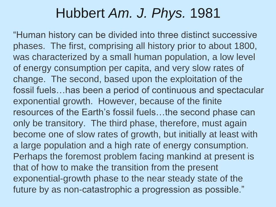
Hubbert Am. J. Phys. 1981

“Human history can be divided into three distinct successive

phases. The first, comprising all history prior to about 1800,

was characterized by a small human population, a low level

of energy consumption per capita, and very slow rates of

change. The second, based upon the exploitation of the

fossil fuels…has been a period of continuous and spectacular

exponential growth. However, because of the finite

resources of the Earth’s fossil fuels…the second phase can

only be transitory. The third phase, therefore, must again

become one of slow rates of growth, but initially at least with

a large population and a high rate of energy consumption.

Perhaps the foremost problem facing mankind at present is

that of how to make the transition from the present

exponential-growth phase to the near steady state of the

future by as non-catastrophic a progression as possible.”

Population Growth Model

Biomass of species:

Constant net growth rate per unit of biomass:

Growth rate of biomass equals inflow minus outflow.

Simplest case: flows are proportional to biomass.

(ingestion & immigration rates minus

excretion, metabolic, emigration, & death rates)

Ý Q QQ rQ

Q

Ý Q

Q r

Exponential Growth

Solution to simple

growth model:

Exponential growth is not sustainable.

Model needs to be adjusted.

Introduce a “crowding” term:

Q Q0ert

Q 2

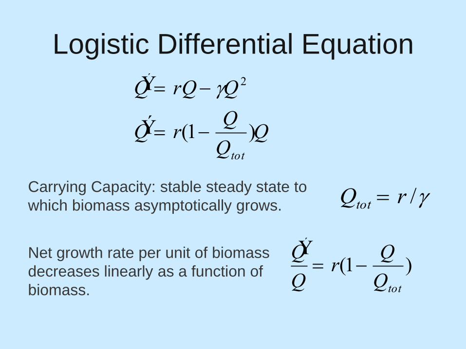
Logistic Differential Equation

Carrying Capacity: stable steady state to

which biomass asymptotically grows.

Net growth rate per unit of biomass

decreases linearly as a function of

biomass.

Ý Q rQ Q 2

Ý Q r(1Q

Qtot

)Q

Ý Q

Q r(1

Q

Qtot

)

Qtot r /

Logistic Growth Curve

Peak at midpoint

time tm occurs when

Q = Qtot/2

Q Qtot

1 er ( tm t )

Ý Q rQtote

r (tm t )

(1 er (tm t ) )2

Logistic Growth Applied to

Oil Production

In 1956 Hubbert applied a logistic growth model to oil production data:

)1(totQ

Qr

Q

P

Q

r

totQ

cumulative oil production (in billions of barrels)

oil production (in billions of barrels per year)

initial production per cumulative production

(in inverse years)

total recoverable oil that ultimately will be produced

(in billions of barrels)

P Ý Q

Is Dependence on Foreign Oil

Inevitable?

Hubbert in 1956 correctly predicted US production would peak in 1970.

Hubbert used the derivative of the logistic growth curve to fit oil production data.

“Decline-from-the-Midpoint”

is observed in US production

0

1

2

3

4

1860 1910 1960 2010

year

P (

bil

lion

barr

els/

yr)

Yearly oil discovery in the lower 48

Deffeyes Hubbert’s Peak Princeton Press 2001

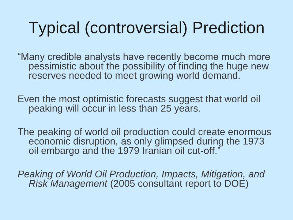
Typical (controversial) Prediction

“Many credible analysts have recently become much more pessimistic about the possibility of finding the huge new reserves needed to meet growing world demand.

Even the most optimistic forecasts suggest that world oil peaking will occur in less than 25 years.

The peaking of world oil production could create enormous economic disruption, as only glimpsed during the 1973 oil embargo and the 1979 Iranian oil cut-off.”

Peaking of World Oil Production, Impacts, Mitigation, and Risk Management (2005 consultant report to DOE)

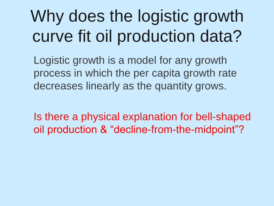
Why does the logistic growth

curve fit oil production data?

Logistic growth is a model for any growth

process in which the per capita growth rate

decreases linearly as the quantity grows.

Is there a physical explanation for bell-shaped

oil production & “decline-from-the-midpoint”?

Deffeyes’ “Explanation”

“…the analogy between population growth

and oil production seems a little odd…The

peculiar part is the analogy between

people having babies and oil wells

begetting additional oil wells. In a crude

sense, oil wells do raise families. Drilling a

discovery well brings on a bunch of new

wells to develop the oil field.”—Deffeyes

Hubbert’s Peak Princeton Press 2001

The Physical Process of Oil

Extraction

Oil extraction is a

pressure driven process.

High pressure water or

gas forces oil through

well.

Oil/water contact line

rises as oil is depleted

and pressure drops until

oil is no longer forced

out.

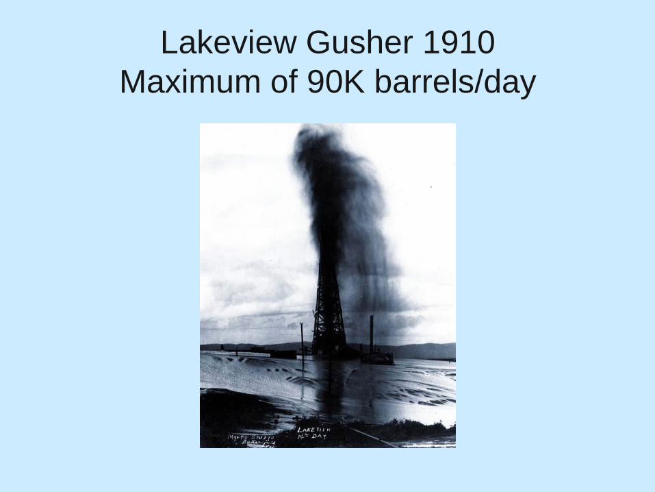
Lakeview Gusher 1910

Maximum of 90K barrels/day

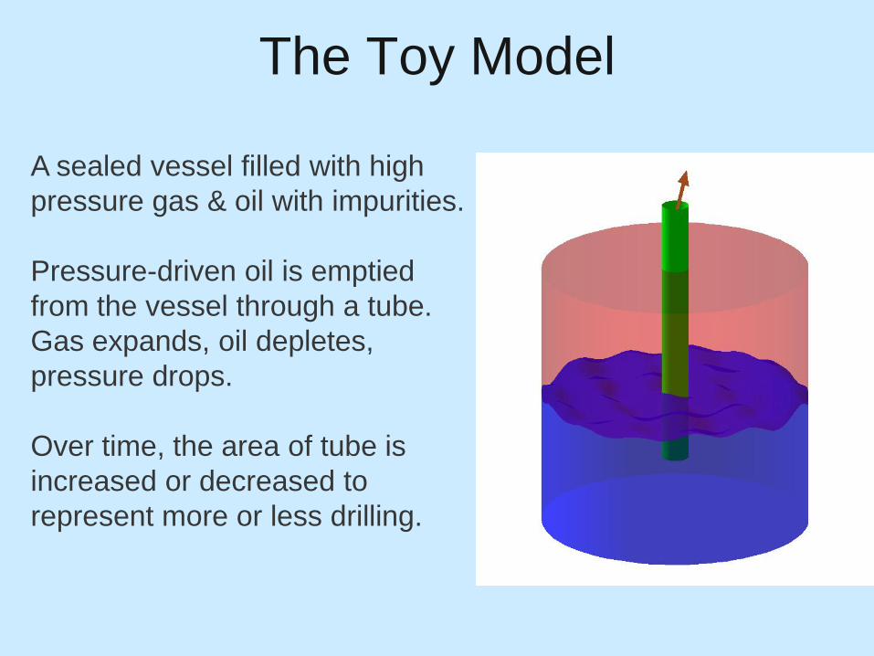
The Toy Model

A sealed vessel filled with high

pressure gas & oil with impurities.

Pressure-driven oil is emptied

from the vessel through a tube.

Gas expands, oil depletes,

pressure drops.

Over time, the area of tube is

increased or decreased to

represent more or less drilling.

Re-injection Toy Model

In real oil reservoirs, water

or gas is re-injected as a

secondary recovery method

to maintain high pressure.

The toy model can be

modified to include re-

injection. Volume of oil and

impurities is kept constant,

but fraction of oil to impurities

decreases.

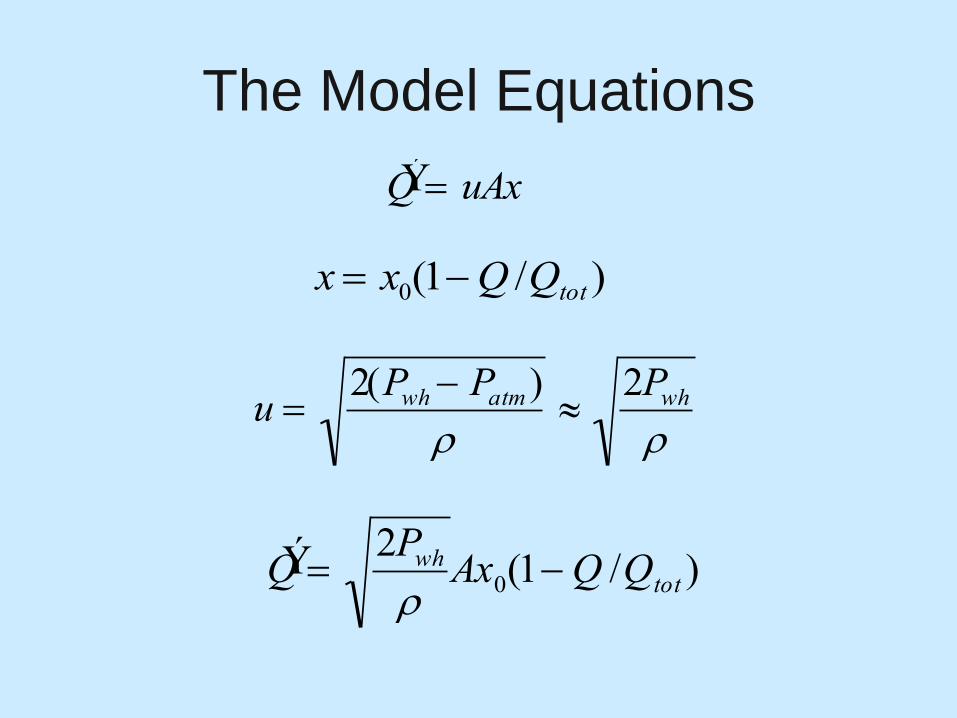
The Model Equations

Ý Q uAx

x x0(1Q /Qtot )

Ý Q 2Pwh

Ax0(1Q /Qtot )

u 2(Pwh Patm )

2Pwh

Behavior of model with several

functions for A

Physical explanation for Peak Oil

In order to increase production, the area of

wells must be increased initially.

However, production must eventually

decrease to zero, regardless of how the

area is varied. For choices of area that

mimic drilling at real oilfields, production is

bell shaped and declines approximately

from the midpoint.

Production peaks before

drilling peaks

Area & production are always positive; f is always positive;

df/dQ is always negative (since the oil fraction is

monotonically decreasing). At Hubbert’s peak the derivative

of area must still be positive, so drilling must still be

increasing when production peaks. Increased drilling can’t

serve as an indicator of future increased production.

Ý Q 2Pwh

Ax0(1Q /Qtot ) Af

Ý Ý Q Ý A f A Ý Q df /dQ 0

Ý A A Ý Q f 1df /dQ Ý A 0

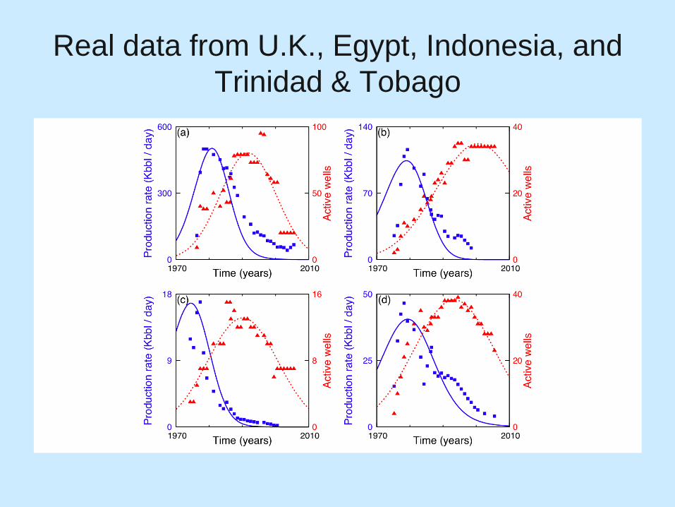
Real data from U.K., Egypt, Indonesia, and

Trinidad & Tobago

Drilling for Oil in the

Arctic National Wildlife Refuge

To drill or not to drill?

Gas prices are rising: we need the oil to

reduce dependency on foreign oil.

ANWR is a pristine ecological preserve that

will be damaged irreparably by drilling.

Hubbert Peak modeling can help examine

the validity of the argument in favor.

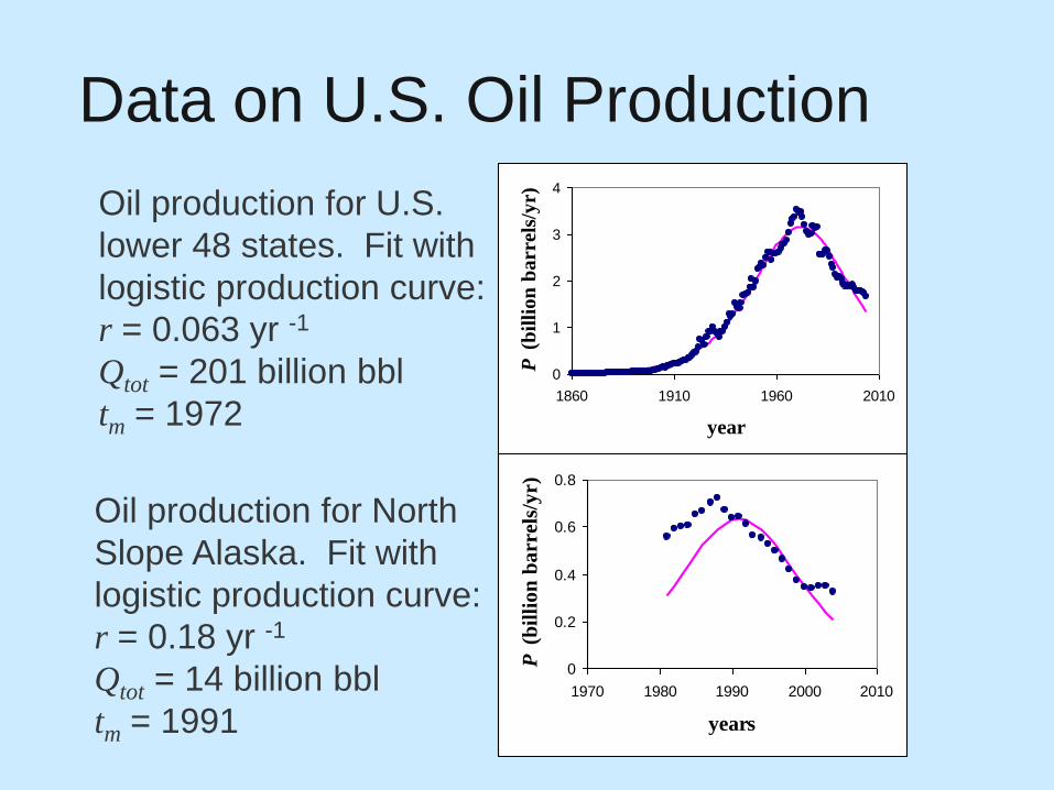
Data on U.S. Oil Production

0

1

2

3

4

1860 1910 1960 2010

year

P (

bil

lion

barr

els/

yr)

0

0.2

0.4

0.6

0.8

1970 1980 1990 2000 2010

years

P (

bil

lion

barr

els/

yr)

Oil production for U.S.

lower 48 states. Fit with

logistic production curve:

r = 0.063 yr -1

Qtot = 201 billion bbl

tm = 1972

Oil production for North

Slope Alaska. Fit with

logistic production curve:

r = 0.18 yr -1

Qtot = 14 billion bbl

tm = 1991

Determining Parameters for

Logistic Production CurvesU.S. without Alaska

0

0.02

0.04

0.06

0 50 100 150 200

Q (billion barrels)

P/Q

(y

r1)

North Slope Alaska

0

0.03

0.06

0.09

0.12

0 5 10 15

Q (billion barrels)

P/Q

(y

r1)

Straight line fits to P/Q vs. Q

y-intercept approximately r

x-intercept approximately Qtot

tm determined by year in

which Q = Qtot/2

ANWR Oil Production

Hypothetical logistic production curve with:

r = 0.12 yr -1 (midway between U.S. & North

Slope Alaska)

Qtot = 10 billion bbl (USGS mean estimate)

tm = 2030 (production begins 2010)

Peak production 300 million bbl/yr (USGS

mean estimate)

Putting It All Together

0

1

2

3

4

1850 1900 1950 2000 2050

year

P (

bil

lio

ns

of

ba

rrel

s/y

r)

U.S. production of oil in billions of barrels per year.

Solid line is a fit to the data projected to 2050.

Dashed line after 2010 is an estimate of total U.S. oil

production if oil is extracted from ANWR.

U.S. Dependence on Foreign Oil

“The key point is that recovering oil from ANWR

cannot stop the overall downward trend in U.S. oil production.

Therefore, recovering this oil is highly unlikely to stop U.S.

dependence on foreign oil from growing. At best it will slow

the rate of increase of this growing dependence. Indeed, we

cannot reasonably expect to end our dependence on foreign

oil by increased access to a new supply of U.S. oil. There

just isn’t enough oil left in the U.S. The discovery of new oil

in the U.S., despite large fluctuations in the data, clearly

peaked decades before oil production peaked in 1970. As

the 21st century unfolds we will become more and more

dependent on foreign oil unless we almost completely

eliminate U.S. demand for oil.”

Conclusions

The logistic growth curve fits real oil production data.

The toy model captures several features of pressure-driven oil extraction.

The model provides physical insight into why oil production is bell shaped & declines from the midpoint.

In the toy model, oil production must peak before the area peaks, which implies increased drilling cannot serve as an indicator of future increased production.

The U.S. cannot drill itself out of an oil shortage.

Papers

Abrams D. M. and R. J. Wiener, 2009: A model of peak

production in oilfields. Accepted, Am. J. Phys.

Wiener, R. J. and D. M. Abrams, 2007: A physical basis

for Hubbert’s decline-from-the-midpoint empirical model

of oil production. Energy and Sustainability, ed. C. A.

Brebbia and V. Popov, WIT Press.

Wiener, R. J., 2006: Drilling for oil in the arctic national

wildlife refuge. Forum on Physics & Society of the

American Physical Society, 35, No. 3.