a three-regime model of speculative behaviour: modelling the evolution of the s&p 500 composite...

A THREE-REGIME MODEL OF SPECULATIVEBEHAVIOUR: MODELLING THE EVOLUTION OF THE

S&P 500 COMPOSITE INDEX*

Chris Brooks and Apostolos Katsaris

We examine whether a three-regime model that allows for dormant, explosive and collapsingspeculative behaviour can explain the dynamics of the S&P 500. We extend existing models ofspeculative behaviour by including a third regime that allows a bubble to grow at a steady rate,and propose abnormal volume as an indicator of the probable time of bubble collapse. We alsoexamine the financial usefulness of the three-regime model by studying a trading rule formedusing inferences from it, whose use leads to higher Sharpe ratios and end of period wealth thanfrom employing existing models or a buy-and-hold strategy.

The evolution of prices in equity markets during the 1920s, the 1980s and the late1990s has puzzled economists and market participants. During these periods,market prices displayed significant growth followed by abrupt market collapses. Itis hard to reconcile this behaviour with the variation of fundamentals during theseperiods and thus two alternative theories have been developed that try to explainwhy stock markets appeared to be moving without fundamental justification. Thefirst approach attributed these abrupt changes in the market trend to a nonlinearrelationship between actual prices and fundamental values. The second approachsupports the view that self-fulfilling expectations and speculative bubbles causedthe significant and increasing divergence of actual prices from fundamental values.Initially, studies on the relationship between actual prices and fundamental

values focused on the indirect identification of speculative bubbles in financialdata; see Shiller (1981); Blanchard and Watson (1982); West (1987); Diba andGrossman (1988). However, indirect tests of bubble presence suffered frompotential problems of interpretation since bubble effects in stock prices could notbe distinguished from the effects of unobservable market fundamentals. For thisreason, bubble tests, which test directly for the presence of a particular bubblespecification on stock market returns, were developed (Flood and Garber, 1980;Flood et al., 1984; Summers, 1986; Cutler et al., 1991; McQueen and Thorley, 1994;Salge, 1997; van Norden and Schaller, 1999). Under these tests, researchers selectthe type of bubble that they suspect might be present in the data and thenexamine whether this form of speculative bubble has any explanatory power forstock market returns.Although several different types of bubbles have been examined in the litera-

ture, periodically collapsing speculative bubbles, first proposed by Blanchard and

* We are grateful to three anonymous referees for extensive comments on a previous version of thisarticle. We are also grateful to Phillip Xu, Ryan Davies, David Oakes, Menelaos Karanasos, Karim Abadir,Apostolos Filippopoulos, Sarantis Kalyvitis and seminar participants at the Department of Economicsand Related Studies at the University of York, and at the Department of International and EuropeanEconomic Studies at the Athens University of Economics and Business for useful comments and sug-gestions. We are responsible for any remaining errors.

The Economic Journal, 115 (July), 767–797. � Royal Economic Society 2005. Published by BlackwellPublishing, 9600 Garsington Road, Oxford OX4 2DQ, UK and 350 Main Street, Malden, MA 02148, USA.

[ 767 ]

Watson (1982), have attracted increasing attention, especially in the late 1990s.Models of periodically collapsing speculative bubbles are able to capture severalstylised characteristics of historical accounts of �manias and panics� (Kindleberger,1989). The common characteristic of many such periods is that prices initiallydiverge from fundamental values in a systematic and increasing fashion. As timepasses, the rate of divergence accelerates and thus prices increase without boundand this exponential trend is followed by a sharp reversal of market prices tofundamental values when market participants realise that the current price level isunsustainable.

In order to examine the presence of periodically collapsing bubbles empiric-ally, researchers in recent years have focused on the construction of directbubble tests that can identify such stochastic bubble processes in financial andmacroeconomic data. More specifically, Evans (1991) and van Norden andSchaller (1993) show how periodically collapsing speculative bubbles can induceregime-switching behaviour in asset returns. Regime switching in asset returnsand speculative behaviour have been linked in several studies. van Norden andSchaller (1993) and van Norden (1996) show that a two-regime speculativebehaviour model has significant explanatory power for stock market and foreignexchange returns during several periods of observed market over and under-valuations. Hall et al. (1998) test for the presence of collapsing speculativebubbles in Argentinean monetary data using a univariate Markov-switching ADFtest and find evidence of a speculative bubble in consumer prices in the periodJune 1986 to August 1988.

van Norden and Vigfusson (1998) compare the van Norden and Schaller (1997)approach with the Hall et al. (1998) switching stationarity test for the presence ofspeculative bubbles and find that both models have significant power in detectingperiodically collapsing speculative bubbles. However, both approaches concen-trate on the explosive phase of the speculative bubble since it is during this phasethat asset prices display significant patterns of bubble behaviour. For this reason,both models are constructed to identify periods of explosive stock market growthfollowed by a sharp reversal. This specification of the bubble tests implicitly as-sumes that a speculative bubble will always display explosive growth, although thiswill be limited for small bubble sizes. This is an unrealistic assumption since thereare periods during which asset prices display constant growth or mimic thebehaviour of fundamentals. During such periods the speculative bubble can beassumed to be �dormant� since it grows at a steady rate. A speculative bubbleprocess that can replicate this switch from a dormant to an explosive state isdescribed in Evans (1991). However, Evans uses this bubble process only in asimulation study and does not provide empirical evidence concerning the pres-ence of such speculative bubbles in asset prices.

In what follows, we try to fill this gap by showing how the van Norden andSchaller (1999) model can be extended to allow for asset price behaviour ofthe form described in Evans. We do this by incorporating a third regime in whichthe bubble grows at the fundamental rate of return. We then examine whether thethree-regime speculative behaviour model has explanatory power for US stockmarket returns. Additionally, we show that other variables, such as abnormally high

768 [ J U L YT H E E CONOM I C J O U RN A L

� Royal Economic Society 2005

volume, can be used in the van Norden and Schaller framework in order to modelthe probability of a bubble collapse more effectively.1

Furthermore, extant research has focused only on the issue of identifying thepresence of speculative bubbles. Although the identification of a speculativebubble is useful in determining whether market participants are rational andwhether markets are efficient, it is also interesting to examine the financial use-fulness of speculative bubble models by testing whether such models can be usedto generate abnormal trading profits or return profiles that typical investors wouldconsider more desirable than those of a buy-and-hold strategy. We do this byformulating a trading rule that exploits information about the implied probabilityof a stock market crash or rally derived from switching regime speculative beha-viour models. This allows us to evaluate the predictive ability of our three-regimemodel against the van Norden and Schaller model in a financially intuitive man-ner: by determining which model can lead to higher Sharpe ratios. Very littleexisting research has been able to pinpoint major market downturns, althoughone exception is Maheu and McCurdy (2000), who use a Markov-switching modelto identify bull and bear runs in stock markets, although they do not examine themodel’s financial usefulness. We also examine the market timing ability of spe-culative behaviour models by comparing the results of the trading rule to those ofa buy and hold strategy and those of randomly generated trading rules. Finally, weemploy a longer sample than in the original van Norden and Schaller study,examining the returns on the S&P 500 for the period January 1888 to January2003.The rest of this paper is organised as follows. In Section 1, we derive the three-

regime speculative behaviour model. Section 2 presents the data and the metho-dology used to construct fundamental values. Section 3 presents the results of thespeculative behaviour models while in Section 4 we examine the out of sampleforecasting ability and profitability of the speculative behaviour trading rules.Section 5 concludes.

1. A Three-Regime Speculative Behaviour Model

An extensive theoretical literature exists concerning the development of rationalspeculative bubbles (Blanchard, 1979; Blanchard and Watson, 1982; West, 1988;Diba and Grossman, 1988; and Kindleberger, 1989). In the Blanchard and Watson(1982) model, the speculative bubble would burst to zero in the collapsing state,and therefore it could not regenerate. The possibility of negative bubbles was alsoexplicitly ruled out. An important recent innovation was the model proposed byvan Norden and Schaller (1999), where the size and probability of bubble collapseare dependent on bubble size and where both positive and negative bubbles arepermitted, and where partial bubble collapses are permissible (the latter are alsoconsidered by Evans (1991) and by Hall and Sola (1993)). van Norden and Sch-aller estimate the model using data on the value-weighted index of all stocks from

1 Brooks and Katsaris (2004) have examined the usefulness of volume as a classifier and predictor ofexcess returns in the context of the van Norden and Schaller (1999) two-regime model.

2005] 769TH R E E - R E G I M E MOD E L O F S P E C U L A T I V E B E H A V I O U R


the Centre for Research on Security Prices (CRSP) database for the period January1926 to December 1989. Their results show that there is non linear predictability instock market returns and that the deviations of actual prices from fundamentalvalues are a significant factor in predicting both the level and the generating stateof returns. They find that the model has explanatory power for several periods ofapparently speculative behaviour of the data, since the probability of a crashincreases significantly prior to large stock market declines while the probability ofa rally is high prior to large stock market advances.

Although the van Norden and Schaller approach can be used directly to test forthe presence of periodically partially collapsing speculative bubbles, it has severallimitations. Firstly, van Norden and Schaller do not provide any information onthe out of sample forecasting ability of their model. Furthermore, their modelprovides limited information as to the likely time of a bubble collapse, since theprobability of a collapse is solely dependent on the bubble size. This leads to longperiods of high probabilities of collapse, when the bubble deviation is persistentlyhigh. Moreover, although the power of the speculative behaviour model to detectbubbles of the form described by Evans (1991) has been examined by van Nordenand Vigfusson (1998), the financial usefulness of this model has not, to ourknowledge, been examined. It would thus be interesting to determine whether thismodel can be used in order to time large market falls. Finally, the van Norden andSchaller model examines only the explosive state of a speculative bubble since it isduring this state that asset prices display apparent bubble behaviour. This impliesthat their model assumes that the bubble will always induce explosive behaviour inasset prices; the asset price will either grow with explosive expectations or willreverse to fundamental values. However, it is possible (and casual observation ofbubbly series provides support for the idea) that speculative bubbles in stockmarkets may alternate between �dormant� and explosive states.2 During the dor-mant state, the bubble grows at the required rate of return without explosiveexpectations since the probability of a crash is zero or negligible, as in the Evans(1991) model. In such periods, the actual returns on the asset are equal to thereturns on the fundamentals, plus a random disturbance and thus actual pricesmimic the behaviour of fundamental values. This bubble behaviour is more con-sistent with a three-regime speculative model. This switching between a dormantbubble state and an explosive bubble state can be observed in the early 1920s, theearly 1950s, the 1960s and the early 1990s amongst other periods, when bubblesalternate between growing at a small steady growth rate and an increasinglyexplosive growth rate. However, as seen from the results of van Norden and Sch-aller, their model will always assign a small but positive probability of the bubblecollapsing and this probability will affect the expected returns on the asset. Thiswill cause a positive bias in the estimates of the probability of collapse at everypoint in time and especially during periods when the bubble displays constantgrowth. It is therefore preferable to construct a speculative behaviour model thatexplicitly allows for dormant periods as well as for explosive bubble growth.

2 Bohl (2000) suggests the use of a threshold autoregressive model in a cointegration framework toseparate periods of deterministic from explosive bubble growth.



We will now show how the van Norden and Schaller model can be extended to athree-regime speculative behaviour model. The latter describes a process in whichthe expected size of the bubble in the next time period can be generated from oneof three regimes: a deterministic (or �dormant�) regime (D), a surviving-explosiveregime (S), and a collapsing-explosive regime (C). It is worth stating at the outsetthat our model, whilst it is a regime-switching model, is not a Hamilton-styleMarkov-switching model, since the probability of being in a particular regime attime t þ 1 does not depend directly on the state at time t. The bubble of the nexttime period can be generated from any of the three regimes. In order to classifythe behaviour into one of the three regimes, several variables may be significant,although the relative size of the bubble is expected to play a predominant role.The model will now be defined.Following Evans (1991), in regime D, the bubble size is small and thus investors

believe that the bubble will continue to grow at a constant mean rate (1 þ i):

Etðbtþ1 Wtþ1 ¼ Dj Þ ¼ ð1þ iÞbt ð1Þ

where bt is the size of the bubble (the difference between the actual andfundamental price) at time t, i is a constant discount rate, and Wt is an unobservedindicator that determines the state in which the process is at time t. This regimeimplies that investors believe that the bubble has a negligible probability ofcollapse and thus they do not expect to be rewarded for this probability with anexcess return. Evans (1991) assumes that once a bubble crosses a certain threshold,it erupts into an explosive regime in which the bubble continues to grow orcollapses to a smaller value. Evans (1991) arbitrarily assumes a threshold value,whereas we model the probability of being in regime D. The probability of being inregime D in time t þ 1 is denoted nt, and is dependent on the bubble’s relative sizeand on other variables observed at time t; this probability will be defined preciselylater. Note that the nt is used to denote the probability of being in regime D ratherthan dt, since the latter conflicts with the standard notation that we adopt later fordividend payments.Even when the bubble is in the dormant regime, investors know that there is a

probability that the bubble might enter an explosive state in which the bubblecontinues to grow with explosive expectations or collapses to a smaller value. Theprobability of being in this explosive state is 1 � nt. In this explosive state, thereare two underlying regimes: the surviving regime that occurs with probability qt

and the collapsing regime that occurs with probability 1 � qt. In the collapsingregime (C), the size of the bubble is given by:

Etðbtþ1 Wtþ1 ¼ Cj Þ ¼ g ðBtÞpat ð2Þ

where g(Bt) is a continuous and everywhere differentiable function such that,g(0) ¼ 0 and 0 � og(Bt)/oBt � 1, Bt is the relative size of the bubble in periodtðBt ¼ bt=pa

t Þ, and pat is the actual asset price at time t. This function is only for

theoretical use and will not be imposed on the data. In the original van Nordenand Schaller model (1993), the bubble size in the collapsing regime is uðBtÞpa

t

where 0 � ou(Bt)/oBt � 1. This implies that in the collapsing regime, theoriginal van Norden and Schaller model states that the bubble in period t þ 1 is



expected to be equal to or smaller than the bubble in period t. We use a slightlydifferent notation and assume that the bubble size is g ðBtÞpa

t where 0 � og(Bt)/oBt � (1 þ i). This implies that the bubble in the collapsing regime is smallerthan the bubble in the �dormant� state and therefore, when the bubble does notyield the required rate of return, it is considered to be in the collapsing state.

From (1) and (2) and since:

Etðbtþ1Þ ¼ nt Etðbtþ1 Wtþ1 ¼ Dj Þ½ �þ ð1� ntÞ qt Etðbtþ1 Wtþ1 ¼ Sj Þ½ � þ ð1� qtÞ Etðbtþ1 Wtþ1 ¼ Cj Þ½ �f g

ð3Þ

we can show that the expected size of the bubble in the surviving regime will be:

Etðbtþ1 Wtþ1 ¼ Sj Þ ¼ ð1þ iÞqt

bt �ð1� qtÞ

qtg ðBtÞpa

t : ð4Þ

At any point in time, the conditional probability of observing the survivingregime in the next time period is given by (1 � nt)qt and the probability ofobserving the collapsing regime is (1 � nt)(1 � qt). Grouping together (1), (2)and (4), the bubble of the next time period will be generated by the followingstochastic process:

btþ1 ¼Mbt with probability nt

M=qtbt � ð1� qtÞ=qtg ðBtÞpat with probability ð1� ntÞqt

g ðBtÞpat with probability ð1� ntÞð1� qtÞ

ð5Þ

where M ¼ (1 þ i) is the gross fundamental return on the security.At this point, it is useful to note three important differences between this model

and the Evans (1991) data generating process. First, we allow for the existence ofnegative (price decreasing) bubbles, and second, in Evans, a strictly positivebubble must cross the arbitrary threshold in order to enter the explosive regime.Finally, he assumes that the probability of collapse in state D is zero, whereas we donot actually impose this on the data.

In (5), we assume that when the bubble is in the dormant regime, the bubblefollows a deterministic process. This is because the probability of observing acollapse when the bubble is in regime D is so small that investors decide to ignoreit Note that our model produces a very small probability of being in regime C inthe next time period, (1 � nt)(1 � qt), if the probability of being in regime D inthe next time period is very high.

We can show that the expected gross total return of the next period, rtþ1, if thebubble is generated by the dormant regime (D), is:3

Eðrtþ1 Wtþ1 ¼ Dj Þ ¼ M : ð6Þ

Equation (6) states that the expected gross return on the asset, if the bubble isgenerated by the dormant regime in the next time period, is equal to the requiredrate of return on the bubble-free asset. Gross returns are calculated as

3 Proofs of the equations are not presented here in the interest of brevity but are available in anappendix from the authors upon request.



rtþ1 ¼ ðP atþ1 þ dtþ1Þ=P a

t and they therefore include dividend payments. However,as the bubble grows, the probability of being in the steady growth regime dimin-ishes and thus the probability of being in the explosive state (surviving or col-lapsing regime) increases. In this explosive state, as the bubble increases, theprobability of being in the surviving state diminishes, causing the probability ofcollapse to increase geometrically. In the explosive state, investors perceive that thebubble can now collapse and thus take into account the probability of a crash. Theexpected return in the surviving regime is:

Etðrtþ1 Wtþ1 ¼ SÞ ¼j M þ ð1� qtÞqt

MBt � g ðBtÞ½ �: ð7Þ

In (7), investors adjust their expectations for the next period return to take intoaccount the probability of collapse. If the bubble collapses, the gross expectedreturn is given by:

Eðrtþ1 Wtþ1 ¼ Cj Þ ¼ M þ g ðBtÞ � MBt : ð8Þ

In (8), the gross return in the collapsing regime is a function of the requiredreturn on the bubbly asset and the relative size of the bubble in the collapsingregime. The magnitude of the return depends on the function g(Bt), a functionthat does not require specification since the model will subsequently be linearised.It is straightforward to see that the above bubble model collapses to the original

van Norden and Schaller model if we set the probability of being in the dormantregime equal to zero. Furthermore, if we fix the probability of survival to a constantvalue and set the bubble size in the collapsing regime equal to zero then the modelcollapses to the original Blanchard and Watson (1982) model. Finally, the prob-ability-weighted expected return on the asset at any point in time is M, and this isalso the ex ante bubble growth rate. This comprises the expected return in state D,which is M, and a return higher than M in state S and lower than M in state C.Nothing has yet been said about the probabilities nt and qt apart from that they

are negative functions of the size of the bubble. Let us examine these probabilitiesin more detail. From the original Evans (1991) model, as the bubble grows, theprobability of being in the dormant regime (D) decreases. Here we consider bothpositive and negative bubbles and therefore we formulate the probability nt as afunction of the absolute size of the bubble. However, the size of the bubble maynot be the only variable that investors examine in order to decide whether thebubble is in the dormant or the explosive state.In order to model the probability of being in the dormant regime in the next

time period, we base our intuition on the results of Harvey and Siddique (2000)and Chen et al. (2001), who find that when returns have been high in the recentpast, the skewness in future returns is more negative. This implies that highaverage returns will tend to be followed by large negative returns. From (6), theexpected bubble returns in the dormant regime are indistinguishable from theexpected fundamental returns. However, when the bubble enters the explosivestate and survives, we know from (7) that it yields increasingly larger returnsthan the bubble-free asset. For this reason, it is plausible to assume that wheninvestors observe larger average actual returns than average fundamental returns



in the near past they will conclude that the bubble must have entered theexplosive state. The probability of being in the dormant regime falls as thebubble grows, so that time spent in the surviving regime will reduce the prob-ability of being in regime D, ceteris paribus, since it tends to increase the size ofthe bubble. This means that large positive returns imply a smaller probability ofbeing in the �dormant� regime in the near future. Chen et al. (2001) find thatthe predictive power of past returns for skewness is larger if one considers thelast six months� returns. They consider actual returns, however, and we want toseparate bubble returns partially from fundamental returns. For this reason, weinclude the spread of the average 6-month actual gross returns over the average6-month fundamental gross returns as a variable in the probability of being inthe dormant regime. It should be expected that the larger the value of thespread, the lower the probability of the bubble continuing to be in the dormantregime. Since we examine both positive and negative bubbles, we take theabsolute values of the averages before we calculate the spread. This ensures thatwhen a negative bubble is entering the explosive state, we correctly identify theexplosive �growth� of such a bubble. Furthermore, this variable will help toidentify periods of steady bubble growth when the estimated bubble deviation isarbitrarily large. This point will be elucidated shortly. In order to ensure thatestimates of the probability of the dormant state are bounded between zero andone, we follow van Norden and Schaller in using a probit specification. Underthis setting, the probability of being in the dormant regime in the next timeperiod is given by:

PrðWtþ1 ¼ DÞ � nt ¼ Xðbn;0 þ bn;B Btj j þ bn;SSf ;at Þ ð9Þ

where X is the standard normal cumulative density function and Sf ;at is the

absolute value of the average 6-month actual returns minus the absolute value ofthe average 6-month returns of the estimated fundamental values.

Turning now to the probability of the bubble surviving in the explosive state(qt), we stated in the previous Section that in the van Norden and Schallermodel this probability is a function of only the absolute size of the bubble. As inmost of the speculative bubble models, their approach assumes that a bubblecollapse is a random event that may or may not be fuelled by the arrival of news.In effect, most rational speculative bubble models implicitly assume that inves-tors randomly organise and decide to sell at the same time thus causing thebubble to collapse. However, although investors can estimate the probability of abubble collapse from the size of the bubble, they still face uncertainty about thetime of the collapse. We therefore conjecture that investors observe other, non-price, variables in an effort to draw inferences about the probable time of col-lapse, and thus to identify the optimal time to exit from the market. Our sug-gestion is that bubble collapses occur because investors observe a signal thatleads them to the conclusion that the market is no longer expecting the bubbleto continue to exist. Once they observe this signal, they start to liquidate theirholdings and thus cause the bubble to collapse. We consider abnormal tradingvolume as a possible signal and thus as a predictor of the time of the bubblecollapse.



The relationship between trading volume and stock returns has been exten-sively researched in the literature; see Karpoff (1987) for a meticulous survey ofthe literature until 1987. Ying (1966) and Morgan (1976) find that largeincreases in volume are usually followed by increased variance of returns, aresult that leads Morgan (1976) to conclude that volume is associated withsystematic risk. One possible explanation for this finding is that trading volumeis a proxy for the degree of disagreement in the stock market, and the reader isreferred to Harris and Raviv (1993), Kandel and Pearson (1995) and Odean(1998) for other models with the same feature. Although Karpoff (1986) claimsthat abnormal volume is not proof of investor disagreement (either ex ante orex post) about information that is available, Shalen (1993) argues that volumeand return volatility have a positive relationship with the ex ante dispersion ofexpectations about future prices. Furthermore, He and Wang (1995) claim ahigh degree of uncertainty about fundamental values leads to an increase inobserved trading volume. Moreover, Marsh and Wagner (2000) state that,especially for the US stock market, abnormal volume can help explain increasesin the size of both the negative and the positive tails of the return distribution.Although they find that this effect is symmetric, Hong and Stein (1999) andChen et al. (2001) claim that divergence of information, approximated byabnormal trading volume, only causes an increase in the negative tail of thefuture return distribution.Based on the above, we propose that abnormally high trading volume is a

signal of changing market expectations about the future of a speculative bub-ble. This implies that abnormal volume signals an increase in the probability ofthe bubble collapsing, thus causing an increase in the probability of observing alarge negative (positive) return if a positive (negative) speculative bubble ispresent. The main difference between our model and the models of price–volume relationship described above is that the latter state that volumeincreases both tails of the distribution of expected returns or it signifies adecrease in the skewness of future returns. We consider abnormal volume as asign that other investors are selling the bubbly asset, although of course,abnormally high volume could also be considered a sign that investors arebuying the bubbly asset.For abnormal volume to signal an imminent bubble collapse would require

the assumption that investors have different endowments implying that thereare agents in the economy that do not hold equity and may decide to do so ata future date. The effect would be the same if the number of investors changesover time. Furthermore, we assume that some investors face short selling con-straints and that in the short run, the supply of equity from firms, throughIPOs and SEOs is limited. The latter assumption, combined with the unwill-ingness of investors to sell the bubbly asset because of the expectation of highreturns in the surviving regime, cause the supply curve to be relatively inelastic.Under this setting, speculative bubbles are a form of �demand side inflation� instock prices.As the bubble continues to grow, the probability of a crash increases and thus

some investors will decide to liquidate their holdings for profit taking or



because they perceive a crash to be imminent. If a sufficiently large number ofinvestors decide to sell the bubbly asset, supply will increase significantly andthus volume will be abnormally high while the rate of increase in prices willslow. This abnormally high volume will signal that a bubble collapse isimminent. Under this setting, we model the probability of the bubble con-tinuing to be in the surviving regime (S) as a negative function of both theabsolute relative size of the bubble deviation, and a measure of abnormalvolume:

PrðWtþ1 ¼ SÞ � qt ¼ Xðbq;0 þ bq;B Btj j þ bq;BV xt Þ ð10Þ

where V xt is a measure of unusual volume in period t.

Grouping all the equations together yields the following nonlinear switchingmodel of gross stock market returns.4

Eðrtþ1 Wtþ1 ¼ Dj Þ ¼ M ð11aÞ

Etðrtþ1 Wtþ1 ¼ SÞ ¼j M þ ð1� qtÞqt

MBt � g ðBtÞ½ � ð11bÞ

Eðrtþ1 Wtþ1 ¼ Cj Þ ¼ M þ g ðBtÞ � MBt ð11cÞ

PrðWtþ1 ¼ DÞ ¼ nt ð11dÞ

PrðWtþ1 ¼ SÞ ¼ ð1� ntÞqt ð11eÞ

PrðWtþ1 ¼ CÞ ¼ ð1� ntÞð1� qtÞ: ð11f Þ

The model described by (11a) to (11f ) is highly nonlinear, so in order toestimate it, we linearise it by taking the first order Taylor series expansion of (11a),(11b) and (11c) around an arbitrary B0 and V x

0 . The resulting linear switchingregression model of gross returns is:

r Dtþ1 ¼ bD;0 þ uD

tþ1 ð12aÞ

r Stþ1 ¼ bS ;0 þ bS ;BBt þ bS ;V V x

t þ uStþ1 ð12bÞ

r Ctþ1 ¼ bC ;0 þ bC ;BBt þ uC

tþ1 ð12cÞ

PrðWtþ1 ¼ DÞ ¼ X bn;0 þ bn;B Btj j þ bn;SSf ;at

� �ð12dÞ

4 A derivation of these equations is available from the authors upon request. The reader may also findit useful to consult to the working paper by van Norden and Schaller (1997) for a derivation of theirmodel, which is available at the Bank of Canada web site: http://www.bankofcanada.ca/en/res/wp97-2.htm.



PrðWtþ1 ¼ SÞ ¼ 1� X bn;0 þ bn;B Btj j þ bn;SSf ;at

� �h iX bq;0 þ bq;B Btj j þ bq;V V x

t

� �ð12eÞ

PrðWtþ1 ¼ CÞ ¼ 1�X bn;0 þ bn;B Btj j þ bn;SSf ;at

� �h i1�X bq;0 þ bq;B Btj j þ bq;V V x

t

� �h i:

ð12f Þ

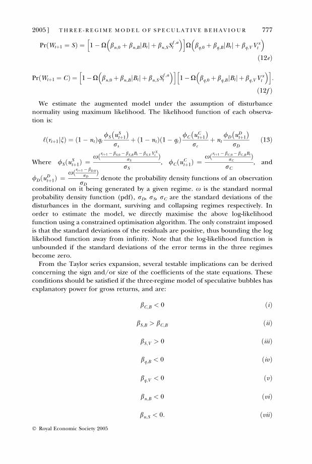
We estimate the augmented model under the assumption of disturbancenormality using maximum likelihood. The likelihood function of each observa-tion is:

‘ðrtþ1 nÞj ¼ 1� ntð Þqt/S uS

tþ1

� �rs

þ 1� ntð Þ 1� qtð Þ/C uC

tþ1

� �rc

þ nt/D uD

tþ1

� �rD

ð13Þ

Where /SðuStþ1Þ ¼

xðrtþ1 � bS;0 � bS;BBt � bS;V V Xt

rSÞ

rS, /CðuC

tþ1Þ ¼xðrtþ1 � bC ;0 � bC ;BBt

rCÞ

rC, and

/DðuDtþ1Þ ¼

xðrtþ1 �bD;0

rDÞ

rDdenote the probability density functions of an observation

conditional on it being generated by a given regime. x is the standard normalprobability density function (pdf), rD, rS, rC are the standard deviations of thedisturbances in the dormant, surviving and collapsing regimes respectively. Inorder to estimate the model, we directly maximise the above log-likelihoodfunction using a constrained optimisation algorithm. The only constraint imposedis that the standard deviations of the residuals are positive, thus bounding the loglikelihood function away from infinity. Note that the log-likelihood function isunbounded if the standard deviations of the error terms in the three regimesbecome zero.From the Taylor series expansion, several testable implications can be derived

concerning the sign and/or size of the coefficients of the state equations. Theseconditions should be satisfied if the three-regime model of speculative bubbles hasexplanatory power for gross returns, and are:

bC ;B < 0 ðiÞ

bS ;B > bC ;B ðiiÞ

bS ;V > 0 ðiiiÞ

bq;B < 0 ðivÞ

bq;V < 0 ðvÞ

bn;B < 0 ðviÞ

bn;S < 0: ðviiÞ



Restriction (i) states that as the bubble increases in size, the expected returnsin the collapsing regime should decrease (increase) if a positive (negative)bubble is present, since the bubble must collapse in regime (C). Furthermore,the speculative behaviour model implies that restriction (ii) must hold sinceas the bubble increases in size we expect the difference of expected returnsacross the surviving and the collapsing regimes to increase as well. Restriction(iii) states that the expected returns in the surviving regime must increase ifabnormal volume is observed since it signals an increase in the probability of abubble collapse. Restrictions (iv) and (v) should hold if our speculative beha-viour model is valid since the probability of the bubble surviving must decreasewhen the absolute size of the bubble or abnormal volume in the market increase.The same holds for restrictions (vi) and (vii) because the probability of being inthe dormant regime (D) must decrease as the bubble grows larger in absolutesize or the returns of the market in the last 6 months are larger than the returnson the fundamental values.

In order to test the power of the model to capture bubble effects in the returnsof the S&P 500, we follow van Norden and Schaller (1999) and test the three-regime speculative bubble model against two alternative models that are nestedwithin the model of speculative behaviour. These alternative models capture styl-ised facts of stock market returns and therefore we examine whether our modelhas any explanatory power beyond these simpler specifications. First, we examinewhether the effects captured by the switching model can be explained by a moreparsimonious model of volatility regimes. In order to test this, we examine thefollowing conditions:

bD;0 ¼ bS ;0 ¼ bC ;0 ð14aÞ

bS ;B ¼ bC ;B ¼ bS ;V ¼ bq;B ¼ bq;V ¼ bn;B ¼ bn;S ¼ 0 ð14bÞ

rD 6¼ rS 6¼ rC ð14cÞ

Restriction (14a) implies that the intercepts across the three state equations arethe same while restriction (14b) states that the bubble deviations, the measure ofabnormal volume and the measure of the spread of actual returns above thefundamental returns have no explanatory power for the returns of period t þ 1 orfor the probability of switching regimes. The later point suggests that there is aconstant probability of switching between a low, medium and high variance regimeas this is stated in restriction (14c).

The volatility regimes model examines the joint hypothesis that the interceptsare the same across the three regimes and that returns and the generating state ofreturns are unpredictable if we use the variables under consideration. It is inter-esting to separate the two hypotheses and to examine whether returns can becharacterised by a simple mixture of normal distributions model that allows bothreturns and variances to differ across the three regimes. This mixture of normalsmodel implies the following restrictions:



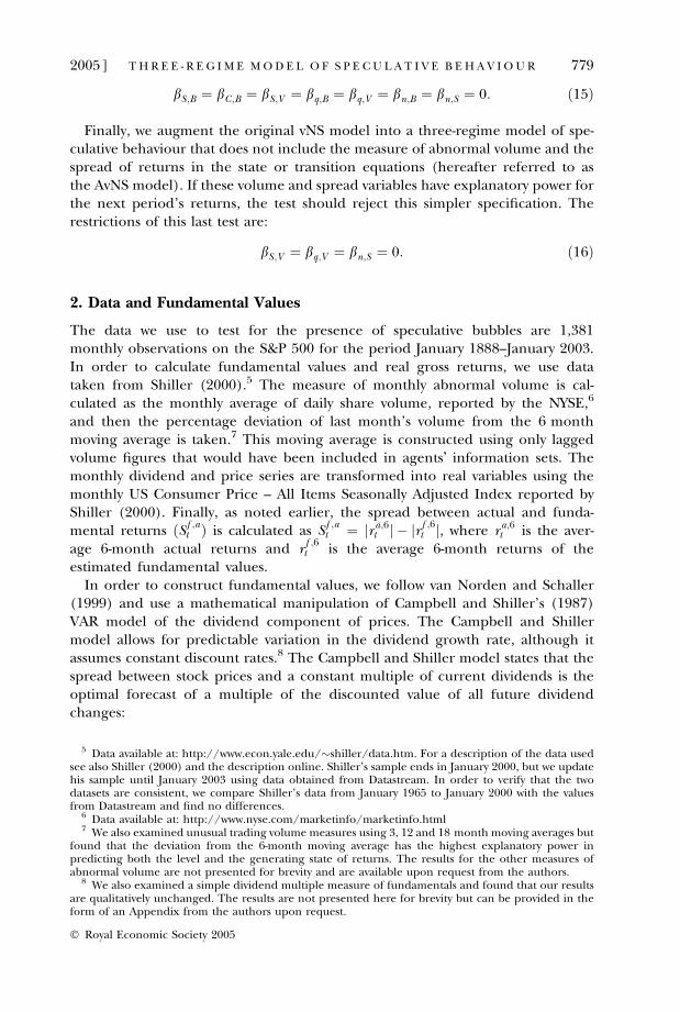
bS ;B ¼ bC ;B ¼ bS ;V ¼ bq;B ¼ bq;V ¼ bn;B ¼ bn;S ¼ 0: ð15Þ

Finally, we augment the original vNS model into a three-regime model of spe-culative behaviour that does not include the measure of abnormal volume and thespread of returns in the state or transition equations (hereafter referred to asthe AvNS model). If these volume and spread variables have explanatory power forthe next period’s returns, the test should reject this simpler specification. Therestrictions of this last test are:

bS ;V ¼ bq;V ¼ bn;S ¼ 0: ð16Þ

2. Data and Fundamental Values

The data we use to test for the presence of speculative bubbles are 1,381monthly observations on the S&P 500 for the period January 1888–January 2003.In order to calculate fundamental values and real gross returns, we use datataken from Shiller (2000).5 The measure of monthly abnormal volume is cal-culated as the monthly average of daily share volume, reported by the NYSE,6

and then the percentage deviation of last month’s volume from the 6 monthmoving average is taken.7 This moving average is constructed using only laggedvolume figures that would have been included in agents� information sets. Themonthly dividend and price series are transformed into real variables using themonthly US Consumer Price – All Items Seasonally Adjusted Index reported byShiller (2000). Finally, as noted earlier, the spread between actual and funda-mental returns ðSf ;a

t Þ is calculated as Sf ;at ¼ jr a;6

t j � jr f ;6t j, where r a;6

t is the aver-age 6-month actual returns and r

f ;6t is the average 6-month returns of the

estimated fundamental values.In order to construct fundamental values, we follow van Norden and Schaller

(1999) and use a mathematical manipulation of Campbell and Shiller’s (1987)VAR model of the dividend component of prices. The Campbell and Shillermodel allows for predictable variation in the dividend growth rate, although itassumes constant discount rates.8 The Campbell and Shiller model states that thespread between stock prices and a constant multiple of current dividends is theoptimal forecast of a multiple of the discounted value of all future dividendchanges:

5 Data available at: http://www.econ.yale.edu/�shiller/data.htm. For a description of the data usedsee also Shiller (2000) and the description online. Shiller’s sample ends in January 2000, but we updatehis sample until January 2003 using data obtained from Datastream. In order to verify that the twodatasets are consistent, we compare Shiller’s data from January 1965 to January 2000 with the valuesfrom Datastream and find no differences.

6 Data available at: http://www.nyse.com/marketinfo/marketinfo.html7 We also examined unusual trading volume measures using 3, 12 and 18 month moving averages but

found that the deviation from the 6-month moving average has the highest explanatory power inpredicting both the level and the generating state of returns. The results for the other measures ofabnormal volume are not presented for brevity and are available upon request from the authors.

8 We also examined a simple dividend multiple measure of fundamentals and found that our resultsare qualitatively unchanged. The results are not presented here for brevity but can be provided in theform of an Appendix from the authors upon request.



st � pft � 1þ i

idt ¼

1þ i

i

X1g¼1

1

ð1þ iÞgEtðDdtþg Þ" #

: ð17Þ

Using the VAR methodology created by Campbell and Shiller, we examinewhether changes in dividends can be forecasted by the spread between prices andthe multiple of current dividends. If the changes in dividends cannot be forecastby the spread, this would imply that investors use only past dividends to formexpectations about future dividends. If, on the other hand, investors include othervariables in their information set then this information will be reflected in pastprices and thus past realisations of the spread. This would imply that the spreadhas power to forecast future dividend changes. Under this approach, the measureof relative bubble size is thus given by:

Bt ¼ 1� st þ ð1þ iÞ=ið Þdt�1

pt: ð18Þ

Figure 1 presents the bubble deviations calculated from (18) for the entiresample (after adjusting for the number of lags). Note that the bubble deviationsare increasingly large in 1929, 1987 and the late 1990s. The bubble deviations aresignificantly negative in 1917, 1932, 1938, 1942 and 1982. Overall, the Campbelland Shiller measure of bubble deviations displays significant short-term variabilitybut also large and persistent broad swings.

–300

–250

–200

–150

–100

–50

0

50

100

1891

1894

1897

1900

1903

1906

1909

1912

1915

1918

1921

1924

1927

1930

1933

1936

1939

1942

1945

1948

1951

1954

1957

1960

1963

1966

1969

1972

1975

1978

1981

1984

1987

1990

1993

1996

1999

2002

Fig. 1. Bubble Deviations of Actual Prices from Campbell and Shiller Fundamental Values.



3. Results

The results of the three-regime model of speculative behaviour are presented inthe first part of Table 1 alongside the results of the vNS model, and the AvNSmodel for comparison. The AvNS model is a three-regime extension of the vanNorden and Schaller model that is equivalent to our three-regime model but doesnot contain any additional variables other than the bubble deviations in the stateand transition equations. The second panel of the Table contains the results of thelikelihood ratio (LR) tests of the restrictions on the coefficients implied by thespeculative behaviour model while the third panel of Table 1 presents the resultsof the likelihood ratio tests of the volatility regimes, mixture of normals, and theextended van Norden and Schaller alternative models.From the first part of Table 1, all the coefficients of the three-regime model

have the expected sign and a financially meaningful magnitude. More specifically,the estimate of the intercept in the dormant regime (bD,0) is 1.0031, and it is highlysignificant as seen from the standard error. This implies that the expected returnin the dormant regime, which is equal to the required fundamental return, is0.31% per month (3.78% on an annual basis). We consider this figure reasonablein terms of real �fundamental� returns, and the corresponding value of this coef-ficient for the AvNS model is quite similar (1.0033), implying a mean return in thesurviving regime of 4.03% on an annual basis.However, when the price series enters the explosive regime, its behaviour becomes

more extreme. The equilibrium gross return in the surviving regime (bS,0), when thebubble size and the measure of abnormal volume are equal to zero, is significantlyhigher than in the dormant regime, 1.18% per month (15.12% on an annualisedbasis). The equilibrium return in the surviving state in the vNSmodel is between theequilibrium returns of the dormant and the surviving regimes in the three-regimemodels. This could be evidence that the equilibrium return in the two-regimemodelis the result of the mixture of the dormant and explosive growth regimes. Turningnow to the equilibrium return in the collapsing state, we can see that the expectedequilibrium return in state C for the three-regime model is �2.16% per month(�23.09% on an annualised basis). This is consistent with the theory of speculativebubbles since the expected return in the collapsing state should be negative.Examining the slope coefficients in the state equations, we note that the

coefficients on the relative bubble size in the surviving and the collapsingregimes (bS,B and bC,B) have the expected signs and are statistically significant atthe 1% level. It is not possible to derive an expected sign for the bubble coef-ficient in the surviving state since the speculative bubble model only implies thatit should be greater in value than the bubble coefficient in the collapsingregime. Nevertheless, we should expect that as the bubble increases in size,investors demand a higher return to compensate them for the increased risk ofbubble collapse. The speculative bubble model requires the return in the col-lapsing regime to be a negative function of the size of the bubble (bC,B < 0)while the coefficient of the bubble size in the surviving regime must be greaterthan the corresponding coefficient in the collapsing regime (bS,B > bC,B). Fromthe second panel of Table 1, we can see that both of these conditions for model



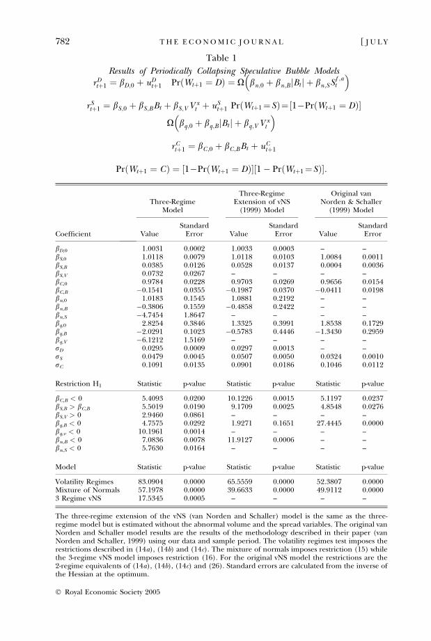
Table 1

Results of Periodically Collapsing Speculative Bubble Modelsr Dtþ1 ¼ bD;0 þ uD

tþ1 PrðWtþ1 ¼ DÞ ¼ X bn;0 þ bn;B Btj j þ bn;SSf ;at

� �r Stþ1 ¼ bS ;0 þ bS ;BBt þ bS ;V V x

t þ uStþ1 PrðWtþ1¼SÞ¼ 1�PrðWtþ1 ¼ DÞ½ �

X bq;0 þ bq;B Btj j þ bq;V V xt

� �r Ctþ1 ¼ bC ;0 þ bC ;BBt þ uC

tþ1

PrðWtþ1 ¼ CÞ ¼ 1�PrðWtþ1 ¼ DÞ�½1� PrðWtþ1¼SÞ�:½

Coefficient

Three-RegimeModel

Three-RegimeExtension of vNS(1999) Model

Original vanNorden & Schaller

(1999) Model

ValueStandardError Value

StandardError Value

StandardError

bD,0 1.0031 0.0002 1.0033 0.0003 – –bS,0 1.0118 0.0079 1.0118 0.0103 1.0084 0.0011bS,B 0.0385 0.0126 0.0528 0.0137 0.0004 0.0036bS,V 0.0732 0.0267 – – – –bC,0 0.9784 0.0228 0.9703 0.0269 0.9656 0.0154bC,B �0.1541 0.0355 �0.1987 0.0370 �0.0411 0.0198bn,0 1.0183 0.1545 1.0881 0.2192 – –bn,B �0.3806 0.1559 �0.4858 0.2422 – –bn,S �4.7454 1.8647 – – – –bq,0 2.8254 0.3846 1.3325 0.3991 1.8538 0.1729bq,B �2.0291 0.1023 �0.5783 0.4446 �1.3430 0.2959bq,V �6.1212 1.5169 – – – –rD 0.0295 0.0009 0.0297 0.0013 – –rS 0.0479 0.0045 0.0507 0.0050 0.0324 0.0010rC 0.1091 0.0135 0.0901 0.0186 0.1046 0.0112

Restriction H1 Statistic p-value Statistic p-value Statistic p-value

bC,B < 0 5.4093 0.0200 10.1226 0.0015 5.1197 0.0237bS,B > bC,B 5.5019 0.0190 9.1709 0.0025 4.8548 0.0276bS,V > 0 2.9460 0.0861 – – – –bq,B < 0 4.7575 0.0292 1.9271 0.1651 27.4445 0.0000bq,v < 0 10.1961 0.0014 – – – –bn,B < 0 7.0836 0.0078 11.9127 0.0006 – –bn,S < 0 5.7630 0.0164 – – – –

Model Statistic p-value Statistic p-value Statistic p-value

Volatility Regimes 83.0904 0.0000 65.5559 0.0000 52.3807 0.0000Mixture of Normals 57.1978 0.0000 39.6633 0.0000 49.9112 0.00003 Regime vNS 17.5345 0.0005 – – – –

The three-regime extension of the vNS (van Norden and Schaller) model is the same as the three-regime model but is estimated without the abnormal volume and the spread variables. The original vanNorden and Schaller model results are the results of the methodology described in their paper (vanNorden and Schaller, 1999) using our data and sample period. The volatility regimes test imposes therestrictions described in (14a), (14b) and (14c). The mixture of normals imposes restriction (15) whilethe 3-regime vNS model imposes restriction (16). For the original vNS model the restrictions are the2-regime equivalents of (14a), (14b), (14c) and (26). Standard errors are calculated from the inverse ofthe Hessian at the optimum.



plausibility are supported by the data. The null hypothesis that the bubblecoefficient in the collapsing regime is equal to zero is rejected at the 5% level(p-value of LR test 0.02), implying that as the bubble size increases, the returnsin the collapsing regime decrease. The opposite holds for negative bubbles sincethey collapse by yielding positive abnormal returns, although it would require anegative bubble size in excess of �15% in order for the returns of the collapsingregime to become positive. Furthermore, we can see that restriction (ii) is sat-isfied since bS,b > bC,b at the 5% level (in the second panel of Table 1 the p-valueof the LR test is 0.019).The three-regimemodel also incorporates abnormal volume in the surviving state

equation. The point estimate of the abnormal volume coefficient in the survivingstate (bS,V) is statistically significant (p-value 0.0061), and has the expected signaccording to condition (iii) (bS,V > 0 at the 10% significance level). This impliesthat as volume increases, expected returns for the next period increase, consistentwith our conjecture that increased abnormal volume signals increased risk.The coefficient estimates of the equation for the probability of being in the

steady growth regime, (12d), are in favour of the three-regime speculative beha-viour model. For the three-regime model, the intercept coefficient (bn,0) impliesthat there is a 15.43% probability of switching to the explosive state when the sizeof the bubble and the spread of actual returns are both equal to zero. Thisprobability is calculated as 1 � X(bn,0) using the point estimates shown in Table 1.The corresponding probability for the AvNS model is 13.83%. However, as thebubble grows, the probability of being in the dormant state in period t þ 1decreases since the coefficients on the absolute bubble size and the spread ofreturns are negative. More specifically, the point estimate of the coefficient on theabsolute bubble size in the equation for the probability of the dormant regime(bn,B) is �0.3806 and is significant at the 5% level. This implies that as the bubblegrows in size, the probability of being in the explosive regime increases.Our model also incorporates the spread of the average six-month actual returns

over the six-month average of fundamental returns in the transition equation. Thisvariable helps to distinguish periods of explosive growth, especially when theestimated bubble deviations are large. The coefficient estimate on the measure ofthe spread (bn,S) is negative, as expected, and significant at the 5% level. Fur-thermore, the LR test results show that the conditions on the signs of the coeffi-cients in the transition equation (vi) and (vii), are satisfied at the 1% and 5% levelrespectively as seen from part two of Table 1. The LR test rejects the hypothesisthat the spread of actual returns does not affect the probability of being in thedormant regime and confirms that the probability of constant growth decreases asthe bubble growth accelerates.Turning now to the probability of being in the surviving regime, the coeffi-

cient estimates of the classifying (12e) for the three-regime model and for theAvNS model are in favour of the presence of periodically collapsing speculativebubbles. As the bubble grows, the probability of being in the surviving regime inperiod t þ 1 decreases since the coefficient on the absolute bubble size isnegative (�2.0291) and statistically significant at the 1% level. Furthermore, theLR test shows that condition (iv), which states that this coefficient should be



negative (bq,B < 0), is satisfied at the 10% level. This is consistent with Evans(1991) and the notion that when the bubble is relatively small, the probability ofthe bubble collapsing is small and thus investors do not take it into account inthe pricing of the asset. As the bubble grows and/or abnormal volume increases,the probability of the bubble collapsing increases geometrically. The point esti-mate of the abnormal volume coefficient in the equation for the probability ofsurvival (bq,V) is negative, as expected, and statistically significant (�6.1212 withp-value 0.0001). The LR test confirms that the probability of the bubble con-tinuing to grow with explosive expectations is a negative function of abnormalvolume. From the above, the probability of the bubble collapsing should increasesignificantly prior to a bubble collapse if our three-regime model is superior atforecasting regime changes. Indeed, in August 1982 when a large negativebubble is present, the probability of the bubble collapsing, estimated from thethree-regime model, increases by 530% to a value of 2.08%. The AvNS model,predicts, for the same month, a probability of collapse of 2.22%, which is only1.3% higher than for the previous month.

The probabilities of being in a given regime calculated from the point estimatesof the three-regime model are presented in Figure 2.9 The corresponding

0

10

20

30

40

50

60

70

80

90

100

1891

1894

1897

1900

1903

1906

1909

1912

1915

1918

1921

1924

1927

1930

1933

1936

1939

1942

1945

1948

1951

1954

1957

1960

1963

1966

1969

1972

1975

1978

1981

1984

1987

1990

1993

1996

1999

2002

Probability of CProbability of SProbability of D

Fig. 2. Probabilities of a Given Regime (D, S, or C) in period t þ 1, Three-Regime Model.January.

9 These probabilities are calculated as Pr(Wtþ1 ¼ D) ¼ nt, Pr(Wtþ1 ¼ S) ¼ (1 � nt)qt, andPr(Wtþ1 ¼ C) ¼ (1 � nt)(1 � qt) using the point estimates of Table 1.



probabilities from the AvNS model are presented in Figure 3. It is apparent thatthe three-regime model incorporating the volume and spread variables yields amore variable probability of being in the steady growth regime, which decreasesconsiderably during periods of significant market advances or declines. Further-more, the probability of being in the collapsing regime increases significantlybefore several bubble collapses, namely August 1929, June 1932, August 1982 andOctober 2000. Note that some of these periods were followed by market rallies.This is because we are also examining price-decreasing bubbles, which collapseyielding positive returns. The probabilities of collapse for both models are alsohigh in other periods that were not followed by bubble collapses. This could beevidence against the speculative bubble model. However, we will show in the nextSection that the three-regime bubble model has significant predictive ability andcan be used to time market reversals.The standard deviations of the residual terms from the three-regime model are

consistent with the theoretical predictions since the standard deviation of the errorterm in the collapsing regime is greater than in the surviving regime. This isbecause bubbles often collapse by yielding extreme negative returns (or positivereturns in the case of price decreasing bubbles). Furthermore, according to Evans(1991) and van Norden and Vigfusson (1998), the standard deviation of the errorsin the dormant regime should be small, since it is periodically collapsing specu-lative bubbles that cause an increase in the variance of returns. The standard

0

10

20

30

40

50

60

70

80

90

100

1891

1894

1897

1900

1903

1906

1909

1912

1915

1918

1921

1924

1927

1930

1933

1936

1939

1942

1945

1948

1951

1954

1957

1960

1963

1966

1969

1972

1975

1978

1981

1984

1987

1990

1993

1996

1999

2002

Probability of CProbability of SProbability of D

Fig. 3. Probabilities of a Given Regime (D, S, or C) in period t þ 1, Extended vNS model.



deviation of the residuals in the steady growth regime is 2.95%, in the survivingregime it is 4.71%, while in the collapsing regime it is 10.91% on a monthly basis.

The third panel of Table 1 presents the results of the LR tests of the augmentedmodel against simpler models that capture well-documented properties of stockmarket returns. The LR test result rejects the volatility regimes alternative speci-fication at the 1% level implying either that the mean returns are different acrossthe three regimes, or that speculative bubbles, abnormal volume and the spread ofactual returns have predictive power for the returns of period t þ 1 or for theprobability of switching regimes. In order to separate the two restrictions, we testthe speculative behaviour model against a mixture of normal distributions modeland the result of the LR test shows that the data reject the mixture of three normaldistributions alternative in favour of the three-regime periodically collapsing spe-culative bubble model. This suggests that the measure of bubble deviations, themeasure of abnormal volume and the spread of actual returns have significantforecasting ability for next period returns and for the probability of switchingregimes. The LR test statistic signifies a rejection of the null of the mixture ofnormal distributions at the 1% significance level. We also examine the three-regime model against the AvNS model in order to see whether abnormal volumeand the spread of actual returns should be used in order to forecast the level andthe generating state of returns. Again, our model rejects this simpler specification.

4. Predictive and Profitability Analysis

Although in the previous Section we showed that the three-regime speculativebehaviour model has significant explanatory power for the S&P 500 returns, theability of this model to forecast historical bubble collapses has not yet beenexamined. In a previous study, van Norden and Vigfusson (1998) examined thesize and the power of bubble tests based on regime-switching models, and foundthat the tests are conservative but have significant power in detecting periodicallycollapsing speculative bubbles of the form described in Evans (1991). However,their technique only examines the econometric reliability of the switching spe-culative bubble model developed by van Norden and Schaller.

In this Section, we will examine the out of sample forecasting ability of the three-regime model and compare it with the forecasting ability of the vNS and the AvNSmodels. We will then investigate whether regime-switching speculative behaviourmodels can be used to determine optimal market entry and exit times. We do thisby creating trading rules based on inferences from the speculative behaviourmodels and test whether such rules can yield abnormal trading profits. Until now,all of the bubble tests that have been created have, to our knowledge, only ad-dressed the problem of bubble identification. We follow a different approach andexamine whether inferences from speculative behaviour models can be used inorder to make financially meaningful forecasts. This approach will also helpexamine the predictive ability of our model against that of van Norden and Sch-aller’s models, in a financially intuitive way.

Several studies have shown that excess stock market returns are partially pre-dictable. One possible explanation is the time variation of required rates of



returns. An alternative explanation is offered by Poterba and Summers (1988) whoclaim that bubbles or fads can induce predictability of excess returns. Note that inthis study we are not trying to predict excess returns. We focus our effort inpredicting the generating state of returns in the next time period, using observablevariables. If the generating state of returns can be predicted then an investor canearn abnormal returns by timing bubble collapses. If our model has no out ofsample forecasting ability over the level or the generating state of returns in thenext time period then this could be taken as evidence against the presence ofbubbles, against our specific speculative behaviour model, or alternatively as evi-dence in favour of market efficiency.In the formulation of the trading rules, we ensure that only information that

would have been available to investors at the time that trades were made is used.For this reason, we cut our sample approximately in half, and estimate the threespeculative behaviour models using data from January 1888 to December 1945.This provides us with initial estimates of the apparent bubble deviations, theexpected returns and the probabilities of being in the three regimes for January1946. Using the point estimates of the three models, we can then calculate theconditional probability of an unusually low and of an unusually high return in thenext period (January 1946). The sample is then updated by one observation withthe models and the probabilities of a crash and of a rally re-estimated. We continuein this fashion and update the sample period used by one month until the end ofthe sample (January 2003) is reached.We consider both the probability of a crash and of a rally to allow for positive

and negative bubbles. Using this rolling estimation with a fixed starting point, weform forecasts for the conditional probabilities of a crash and of a rally using onlyinformation that is available to investors up to that point in time. The conditionalprobability of a crash is calculated using the following equation:

Pr rtþ1 < Kð Þt ¼ ntxK � bD;0;t

rD;t

� �

þ ð1� ntÞ qtxK � bS ;0;t � bS ;B;tBt � bS ;V ;tV

xt

rS ;t

� ��

þð1� qtÞxK � bC ;0;t � bC ;B;tBt

rC ;t

� �� ð19Þ

where nt ¼ X(bn,0,t þ bn,B,t|Bt| þ bn,S,tSt), and qt ¼ Xðbq;0;t þ bq;B;t jBt j þ cq;V ;tVx

t Þ.The time subscripts attached to the speculative model coefficients denote theestimated values of the coefficients using data only up to and including time t. In(19), K is the threshold below which a return is classified as a crash and this isdefined as k ¼ lt � 2(rr,t), where lt is the mean of past gross returns until time t,and rr,t is the standard deviation of past gross returns until time t. The conditionalprobability of observing an extreme positive return of at least two standarddeviations above the mean of past returns in period t þ 1 can be definedaccordingly.The probabilities of a crash calculated using the three-regime model and using

the vNS model are presented in Figure 4 together with markers to signify the 20



largest negative 1-month and 3-month returns observed for the S&P 500 in thefollowing month. In the top part of the Figure, we plot the logarithm of the realS&P 500 index and the logarithm of the Campbell and Shiller (1987) fundamentalvalues. At this point, it should be noted that we have allowed for partial collapses inthe specification of the bubble model and therefore a bubble may partially col-lapse for several periods before starting to grow again. For this reason, we alsoexamine the probability of a crash (rally) against the top 20 3-month negativereturns as well as the top 20 draw-downs. A draw-down is defined as the cumulativereturn from the last local maximum to the next local minimum of the S&P 500Index and thus refers to cumulative continuous losses. From Figure 4, it is evidentthat the probability of a crash increases during several periods when a bubble issuspected to be present but more importantly it is high before several of the 20largest 1-month declines of the S&P 500 including 1959, 1961, 1970, 1974 and2000. All of these periods are followed by a strong correction in stock price levels.

In Figure 5, we present the conditional probability of a rally calculated from thethree-regime model and from the vNS model with markers to signify the 20 largest1-month, 3-month and consecutive market advances. The 20 largest consecutivemarket advances (�draw-ups�) are defined as the 20 largest consecutive positivereturns, defined as the return from the last local minimum to the next local maxi-mum. It is clear that the probability of a rally increases dramatically during severalperiodswhenanegativebubble appears tobepresent, especially in1949–50 and1982.Again, theprobability of a rally estimated from the three-regimemodel is significantlymore variable than the corresponding probability derived from the vNS model.

However, there are several periods during which both probabilities increasesimultaneously, thus damping the effects we seek to observe, namely the condi-tional probability of a crash and of a rally in the next period. This is because the

0

2

4

6

8

10

12

14

16

18

20

1946

1948

1950

1952

1954

1956

1958

1960

1962

1964

1966

1968

1970

1972

1974

1976

1978

1980

1982

1984

1986

1988

1990

1992

1994

1996

1998

2000

2002

Prob

abili

ty o

f a

Cra

sh (

%)

1.00

1.50

2.00

2.50

3.00

3.50

Log

Ind

ex &

Fun

dam

enta

l Val

ues

3 Regime Probability of a CrashVan Norden & Schaller Probability of a Crash20 Largest 1 Month Declines20 Largest 3 Month Declines20 Largest Draw DownsLog Real IndexLog CS Rolling Fundamental Values

Fig. 4. Probabilities of a Crash from the Three-Regime and the van Norden and Schaller Models.



conditional distribution of expected returns is a mixture of a low variance (dor-mant state), medium variance (surviving state) and a high variance (collapsingstate) distribution. As the relative size of the bubble increases, the weight of thehigh variance distribution increases and thus both tails increase at the same time.Furthermore, we note several spikes in the probabilities of a crash and of a rallythat where not immediately followed by a market collapse or a market rally. This iswhat we would expect to see from a model of speculative behaviour, since if thetime of the crash could be forecast with great accuracy then this would violate theassumption of investor rationality, since if an investor knows that the bubble willcollapse in a month he will sell now or at any point until the time of collapse. Thiswould rule out speculative bubbles all together since actual prices could neverdeviate from fundamental values in this setting.We proceed to form a trading rule based on the models and to calculate the risk

and return of these rules at each point in time. We then evaluate the trading rules�results by calculating the profits (or losses) that an investor would have made if hewere using the three-regime model in an effort to time large market movementsfrom January 1946 to January 2003 and compare the returns to the results of thevNS model and with returns generated by random trading rules. The trading rulestates that when the probability of a crash (rally) crosses the upper 90th percentileof its historical values, the investor should sell (buy) the index, investing entirewealth in a risk-free asset (equities),10 and maintain this position until the prob-ability of a crash (rally) becomes lower than its historical median value, i.e. until the

0

2

4

6

8

10

12

14

16

18

2019

4619

4819

5019

5219

5419

5619

5819

6019

6219

6419

6619

6819

7019

7219

7419

7619

7819

8019

8219

8419

8619

8819

9019

9219

9419

9619

9820

0020

02

Date

Prob

abili

ty o

f a

Ral

ly %

1.00

1.50

2.00

2.50

3.00

3.50

Log

Ind

ex &

Fun

dam

enta

l Val

ues

3 Regime Probability of a RallyVan Norden & Schaller Probability of a Rally20 Largest 1 Month Advances20 Largest 3 Month Advances20 Largest Draw UpsLog Real IndexLog CS Rolling Fundamental Values

Fig. 5. Probabilities of a Rally from the Three-Regime and the van Norden and Schaller Models.

10 The risk-free rate for the period January 1946 to January 2003 is taken to be the monthly con-tinuously compounded yield on 3-Month Treasury Bills. The data are taken from the Federal ReserveBank of St Louis web site http://www.stls.frb.org/fred/data/irates.html.



bubble deflates. We use the median in order to avoid any unwanted influence fromextraordinarily large probabilities of a crash and of a rally observed during thesample period (especially 1929–33). When the appropriate probability becomeslower than its historical median value, entire wealth should be invested in the S&P500 Index. We include the probability of a rally in the strategy since an investorshould buy if there is a negative bubble and the probability of a rally is greater thanthe 90th percentile of its historical values. In order to ensure that we are not usingany information that was not available to the investor at the time of the trade, wecalculate the median value and the top 90th% value using a rolling window with afixed starting point in January 1888. Focusing on the 90th percentile is somewhatarbitrary, but represents a trade-off between using too high a cut-off, which willencourage the investor to remain in the market when the bubble has a historicallyhigh probability of collapse, while using too low a cut-off will lead the investor out ofthe market too frequently, resulting in missed bull market opportunities. Ourresults are not qualitatively altered if an 80% or 95% cut-off is employed instead.

We compare the three-regime model with the vNS model by calculating the totalholding period return for every month and examine the mean, standard deviation,skewness and kurtosis of each trading rule’s return distribution. We note thenumber of trades that the rule has generated over the trading period in order toadjust trading profits for transaction costs, and we also note the percentage of timethat an investor following the rule would have invested in equities. To take intoaccount transaction costs, we assume a 0.5% round trip cost.11 We then comparethe trading performance of the three-regime model with the results of the vNSmodel and with the results of a simple buy and hold strategy.

Furthermore, in order to examine the statistical significance of the profitsgenerated from the trading rule, we form 10,000 long random trading rules cre-ated by randomly generating series of zeros and ones, the length of which is equalto the number of months in our trading sample (January 1946–January 2003, or685 months) using a binomial distribution. The probability of success (i.e. of abinomial draw of one) is set equal to the percentage of time that trading rulewould suggest the investor to be in the market. We use this probability of successbecause it yields random trading rules with comparable average holding periods toour trading rules. In order to test for the statistical significance of the bubble rules,we compare the returns and the other moments of the returns� distributions withthose of the random rules and if our model yields a profit larger than 90%, 95% or99% of the random trading rules we can conclude that our abnormal profits arestatistically significant at the 10%, 5% and 1% levels respectively. Finally, for everytrading rule generated from the bubble models and the random rules, we calculatethe wealth that an investor would have accumulated by January 2003 from an initialinvestment of one dollar in January 1946.

Table 2 contains the trading rule results for the three-regime and for the vNSmodels, and also presents the results of the buy and hold strategy. The values in

11 It should also be noted that the use of our trading rule may have adverse tax effects as a result ofthe realisation of capital gains, and therefore that the rule and the trading return results described aremore relevant to tax-sheltered accounts that do not have such tax liabilities.



Tab

le2

Spec

ula

tive

Bu

bble

Mod

els’

Tra

din

gR

ule

sR

esu

lts

agai

nst

Ran

dom

lyG

ener

ated

Tra

din

gR

ule

san

dth

eB

uy

and

Hol

dSt

rate

gy.

Strategy

Mean

Return

(%)

Stan

dard

Deviation

(%)

Skew

ness

Excess

Kurtosis

Endof

Period

Wealth

Sharpe

Ratio

%ofTim

ein

the

Marke

t

Number

of

(roundtrip)

Trades

Adjusted

Sharpe

Ratio

Adjusted

End

ofPeriod

Wealth($)

Buyan

dHold

0.60

3.56

�0.58

1.68

$39.81

0.15

5010

0.00

%0

0.15

3239

.81

RiskFree

Investmen

t0.05

0.44

�3.98

39.62

$1.42

–0.00

0–

–

3-Reg

ime

Model

0.66

(0.21)

2.41

(1.89)

0.45

(0.15%

)2.88

(0.01%

)$5

3.80

(0.05%

)0.25

06(0.02%

)58

.10

470.23

3747

.70

Original

vNS

Model

0.39

(60.52

)2.10

(51.15

)�0.45

(75.55

%)

10.99(0.03%

)$1

2.14

(65.13

%)

0.16

01(55.56

%)

33.87

190.14

8611

.55

Tradingrulesareform

edbased

ontheco

nditional

probab

ilityofacrashwhen

apositive

bubble

ispresentan

dtheco

nditional

probab

ilityofarallywhen

aneg

ative

bubble

ispresent.Theinvestoreither

placeshisen

tire

wealthin

theS&

P50

0Composite

Index

orin

the3-month

U.S.T

reasury

Bill.Theen

dofperiodwealthisthe

real

valueoftheinvestor’sportfolioin

January20

03iftheinitialvalueoftheportfolioin

January19

46was

$1.00.

Allthenumbersan

dthereturnsarein

real

term

s.Figuresin

paren

theses

showthepercentile

rankingofthetrad

ingrule

relative

to10

,000

random

trad

ingruleswithan

equal

percentage

oftimeinvested

inthe

index

.Themeanreturn

istheaveragemonthly

real

totalreturn

fortheperiodJanuary19

46–Jan

uary20

03.an

dthestan

darddeviationofreturnsisthestan

dard

deviationoftotalreturns.TheSh

arperatioistheratioofthemeanex

cess

return

ofagiventrad

ingrule

overtheco

rrespondingstan

darddeviationofreturns.The

percentage

oftimein

themarke

tisthepercentage

ofmonthsthetrad

ingrule

producedahold

sign

aloutofthe68

5monthsin

thesample.Thead

justed

endof

periodwealthshowstheen

dofperiodwealthnet

oftran

sactionco

sts.Transactionco

stsareassumed

tobe0.5%

per

roundtrip

onthetotalvalueofthetrad

e.



parentheses are the percentage of random rules that lead to higher averagereturns, lower standard deviation, higher skewness etc. Lower values inside par-entheses denote a more superior relative performance of the speculative beha-viour model trading rule against the random trading rules.

From the results, we see that the three-regime model trading rule yields higherSharpe ratios and a larger end of period wealth compared to the vNS model. Morespecifically, if an investor used the three-regime speculative behaviour model withthe Campbell and Shiller (1987) measure of fundamental values throughout theperiod examined, he would have received an average return of 0.66% per month(8.2% on an annualised basis) with a standard deviation of 2.41%. If, however, theinvestor used the vNS model, he would only receive an average return of 0.39% permonth with a standard deviation of 2.10%. Furthermore, the end of period wealthfor the three-regime model is consistently higher than that of the original vNSmodel, and the buy and hold strategy.

The three-regime model also clearly outperforms 99% of the randomly gener-ated trading rules in terms of the Sharpe ratio and end of period wealth, signifyingthat the three-regime model has significant market timing ability. Application ofthe vNS model only manages to beat 35% of the randomly generated trading rulesin end of period wealth and 45% of the random strategies in terms of the Sharperatio. Moreover, the end of period wealth and the Sharpe ratio of the three-regimemodel trading rule is higher than the Sharpe ratio of the buy and hold strategy,although this superiority with respect to the buy and hold strategy fades somewhatif we examine the total wealth and the Sharpe ratio after we take into account thetransaction costs involved. Note that the three-regime model requires considerablyhigher number of trades than the original van Norden and Schaller model.

This higher end of period wealth of the three-regime model is achieved withhigher skewness and lower kurtosis coefficients than the vNS model. Both of thesehigher moments of the distribution (i.e. the third and fourth moments) of thethree-regime model returns would be more desirable to investors under somefairly weak assumptions concerning the shape of investor utility functions (seeScott and Horvath (1980) for higher moment preferences and Kraus and Lit-zenberer (1976), and references therein for skewness preference in asset pricing).This arises since rational investors desire high positive values of odd moments (i.e.mean and skewness) and the smallest possible values of even moments (varianceand kurtosis). Intuitively, skewness measures the relative size of the left-hand tail ofthe return distribution, and a large left tail implies a greater probability of largelosses. Similarly, kurtosis is a measure of tail-fatness and, all other things beingequal, a large kurtosis again implies a higher probability of large losses.

The above results show that if an investor used the three-regime model toidentify optimal market entry and exit points, he would have earned a higherSharpe ratio and end of period wealth in January 2003 than if he was using the vNSmodel or following a passive buy and hold strategy. In Figure 6, we plot the realS&P 500 Composite Index and the net excess wealth of the three-regime modeltrading rule as a percentage of the wealth of the buy and hold strategy. On the plotof the S&P 500, we place markers that signify entry and exit times that the three-regime model trading rule has generated. In this Figure, investor wealth has been



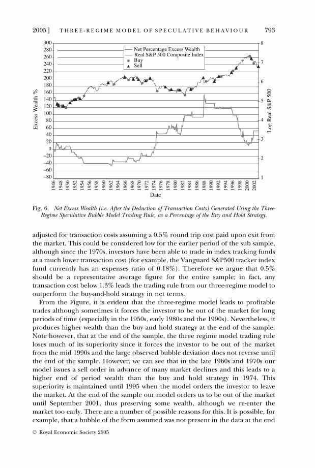
adjusted for transaction costs assuming a 0.5% round trip cost paid upon exit fromthe market. This could be considered low for the earlier period of the sub sample,although since the 1970s, investors have been able to trade in index tracking fundsat a much lower transaction cost (for example, the Vanguard S&P500 tracker indexfund currently has an expenses ratio of 0.18%). Therefore we argue that 0.5%should be a representative average figure for the entire sample; in fact, anytransaction cost below 1.3% leads the trading rule from our three-regime model tooutperform the buy-and-hold strategy in net terms.From the Figure, it is evident that the three-regime model leads to profitable

trades although sometimes it forces the investor to be out of the market for longperiods of time (especially in the 1950s, early 1980s and the 1990s). Nevertheless, itproduces higher wealth than the buy and hold strategy at the end of the sample.Note however, that at the end of the sample, the three regime model trading ruleloses much of its superiority since it forces the investor to be out of the marketfrom the mid 1990s and the large observed bubble deviation does not reverse untilthe end of the sample. However, we can see that in the late 1960s and 1970s ourmodel issues a sell order in advance of many market declines and this leads to ahigher end of period wealth than the buy and hold strategy in 1974. Thissuperiority is maintained until 1995 when the model orders the investor to leavethe market. At the end of the sample our model orders us to be out of the marketuntil September 2001, thus preserving some wealth, although we re-enter themarket too early. There are a number of possible reasons for this. It is possible, forexample, that a bubble of the form assumed was not present in the data at the end

–80–60–40–20

020406080

100120140160180200220240260280300

1946

1948

1950

1952

1954

1956

1958

1960

1962

1964

1966

1968

1970

1972

1974

1976

1978

1980

1982

1984

1986

1988

1990

1992

1994

1996

1998

2000

2002

Date

Exc

ess

Wea

lth %

1

2

3

4

5

6

7

8

Log

Rea

l S&

P 50

0

Net Percentage Excess WealthReal S&P 500 Composite IndexBuySell

Fig. 6. Net Excess Wealth (i.e. After the Deduction of Transaction Costs) Generated Using the Three-Regime Speculative Bubble Model Trading Rule, as a Percentage of the Buy and Hold Strategy.



of the sample period or it is possible that the model used to estimate fundamentalvalues is not adequate and does not capture fundamentals precisely.

5. Conclusions

In this study we have presented a three-regime switching speculative behaviourmodel that is able to capture speculative dynamics present in the S&P 500 Com-posite Index. The model is based on the models developed by van Norden andSchaller (1999) and Evans (1991). We show how the original van Norden andSchaller model can be augmented to include a third regime in which the bubblegrows at the fundamental rate of return. In this dormant state, the bubble beha-viour is very different than in the explosive state since the probability of collapse isnegligible. We show that, as in van Norden and Schaller, the magnitude of thedifference between actual prices and fundamental values is a significant predictorand classifier of returns. Furthermore, we show that other variables such asabnormally high volume and the difference of average actual returns from averagefundamental returns can assist in classifying future returns into the three regimes.

Using data on the S&P 500 for the period January 1888–January 2003, we findthat the speculative behaviour model has significant explanatory power for thenext month’s returns. More specifically, as the bubble grows in size and yieldshigher returns, the probability of being in the explosive regime in the next timeperiod increases, and thus the expectation of bubble growth is adjusted to com-pensate for the now higher probability of a bubble collapse. In the explosive state,the size of the bubble deviation and the measure of abnormal volume help inidentifying the probability of observing a bubble collapse. We find that theprobability of observing an extreme negative return, of at least two standarddeviations below the historical mean of returns, increases significantly when apositive bubble is present and abnormal volume is high. When the three-regimemodel is tested against more parsimonious and established alternatives such asmixtures of normal distributions, volatility regimes and a three-regime extensionof the original model of van Norden and Schaller, it appears that our model’sspecification captures additional information present in the data and classifiesreturns in the switching regime framework more effectively.

We test the out-of-sample forecasting ability of the three-regime model and ofthe van Norden and Schaller model in a financially intuitive way by constructingtrading rules based on inferences concerning the conditional probability of a crashand of a rally, and analysing the returns obtained with the use of the original tworegime speculative behaviour model and of our three-regime extension. Weexamine the timing ability of the bubble models by comparing the returns of thespeculative bubble model trading rules with the returns on 10,000 randomlygenerated trading rules that have the same average proportion of the sampleperiod invested in equities. We find that the three-regime model can consistentlylead to higher Sharpe ratios than the vNS model, the randomly generated tradingrules, and the buy and hold strategy, although some of this superiority fades whenwe take into account the transactions costs involved. Thus, whilst our model is nota �money machine�, its usefulness lies in helping to protect investors from



downside risk if they are willing to pay the associated transactions costs, akin to thepurchase of a protective put. Nevertheless, we must note that there are severallimitations of the switching regime speculative bubble models employed here andelsewhere, which provide scope for further research.First, although the speculative behaviour models presented are considered as

direct tests for the presence of periodically collapsing speculative bubbles, in effectthey examine the presence of a particular form of regime switching behaviourdictated by simple models of collapsing speculative bubbles. It is possible that thisregime switching behaviour may be caused by expected shifts in the evolution offundamentals that are not realised or any other factor that causes regime switchingin asset returns (van Norden and Vigfusson, 1998). However, this is the problem ofany parametric econometric model: the behaviour of a dependent variable that theeconometrician attributes to a particular variable may be caused by anotherunobservable variable.Furthermore, although we allow for the time variation of the dividend growth

rate, we assume that the discount rate is constant in the construction offundamental values. However, the time variation of expected returns has beenwell documented and thus it would be interesting to determine whether spe-culative behaviour models are robust against specifications of fundamentals thatallow for predictable variation in the discount rate. Moreover, our fundamentalvalues are dividend based and there is evidence that companies in the 1990s haveshifted to low dividend payout policies. This could be a contributory factor in thedevelopment of the apparently large bubble deviation estimated in the late1990s. It is also worth noting that anecdotal evidence suggests that when a newsector appears in the economy, stock markets display significantly higher growthrelative to dividend-based fundamentals. However, when these new sectorsbecome mature, stock market prices appear to revert to their dividend-basedfundamentals.Zeira (1999) presents a model of stock market booms and crashes caused by

the uncertainty investors face about fundamental values. In effect, market boomsare caused by informational overshooting when new technologies are imple-mented in the production process and the limit of such technologies is un-known. Once the limit of this �new� technology is reached, market participantsrealise that no further growth is possible and thus cause market prices to crash.This model can be transformed to explain market booms and crashes using thearrival of new investors to the market (�greater fools�) or the liberalisation ofmonetary policy by central banks. Zeira claims that this model is capable of partlyexplaining the booms and crashes of 1929, 1987 and the boom of the Infor-mation Technology Era. Greenwood and Jovanovic (1999) and Hobijn andJovanovic (2000) present a model of technological change that can replicatebooms and crashes observed in financial data and can explain stock marketvaluations during the last 25 years. The main suggestion of the model is that newtechnologies destroy old, incumbent firms once the success of the new tech-nology is made known to the market. Since new technologies are rarely formedby listed companies, and because listed companies usually resist their imple-mentation, stock market valuations are depressed once new technologies are



invented. This is because once small innovative firms are listed on the market,investors shift their attention to such companies and neglect �old� technologyfirms that have lower growth potential.

Models of the form developed here could find a number of useful applicationsin other areas of finance. Regime-switching speculative behaviour models could beused, for example, in portfolio construction or in the computation of value at risk(VaR). The academic literature on the latter is now large and well developed – see,for example, Billio and Pelizzon (2000), who employ a multivariate regimeswitching approach to calculate accurate value at risk estimates for Italian stocks,or Jorion (2000) and the references therein. Value at risk essentially involves anestimation of the cost of extreme losses that occur with a certain probability (e.g.,1%), and our model could be used in such calculations. It would also be of interestfor future research to examine the accuracy of the forecasts of the density ofreturns using the probability integral transform.

Cass Business School

Date of receipt of first submission: May 2002Date of receipt of final typescript: July 2004

ReferencesBillio, M. and Pelizzon, L. (2000). �Value at risk: a multivariate regime switching approach�, Journal of

Empirical Finance, vol. 7, pp. 531–54.Blanchard, O.J. (1979). �Speculative bubbles, crashes and rational expectations�, Economics Letters, vol. 3,

pp. 387–9.Blanchard, O.J. and Watson, M.W. (1982). �Bubbles, rational expectations and financial markets�, NBER

Working Paper Series, No 945, pp. 1–30.Bohl, M.T. (2000). �Periodically collapsing bubbles in the US stock market�, Working Paper, Department

of Economics, European University Viadrina Frankfurt (Oder).Brooks, C. and Katsaris, A. (2004) �Trading rules from forecasting the collapse of speculative bubbles for

the S&P 500 Composite Index� forthcoming; Journal of Business.Campbell, J. and Shiller, R. (1987). �Cointegration and tests of present value models�, Journal of Political

Economy, vol. 95, pp. 1062–88.Chen, J., Hong, H. and Stein, J.C. (2001). �Forecasting crashes: trading volume, past returns and

conditional skewness in stock prices�, Journal of Financial Economics, vol. 61, pp. 345–81.Cutler, D.M., Poterba, J.M. and Summers, L.H. (1991). �Speculative dynamics�, Review of Economic Studies,

vol. 58, pp. 529–46.Diba, B.T. and Grossman, H. I. (1988). �Explosive rational bubbles in stock prices?�, American Economic

Review, vol. 78, pp. 520–30.Evans, G.W. (1991). �Pitfalls in testing for explosive bubbles in asset prices�, American Economic Review,

vol. 81, pp. 922–30.Flood, R.P. and Garber, P. (1980). �Market fundamentals versus price level bubbles: the first tests�,

Journal of Political Economy, vol. 88, pp. 745–70.Flood, R.P., Garber, P. and Scott, L. (1984). �Multi country tests for price level bubbles�, Journal of

Economic Dynamics and Control, vol. 8, pp. 329–40.Greenwood, J. and Jovanovic, B. (1999). �The information-technology revolution and the stock market�,

American Economic Association Papers and Proceedings, vol. 89, pp. 116–22.Hall, S.G. and Sola, M. (1993). �Testing for collapsing bubbles; an endogenous switching ADF test�,

Discussion Paper 15–93, London Business School.Hall, S.G., Psaradakis, Z. and Sola, M. (1998). �Detecting periodically collapsing bubbles: a Markov-

switching unit root test�, Journal of Applied Econometrics, vol. 14, pp. 143–54.Harris, M. and Raviv, A. (1993). �Differences of opinion make a horse race�, Review of Financial Studies,

vol. 6, pp. 473–506.Harvey, C.R. and Siddique, A. (2000). �Conditional skewness in asset pricing tests�, Journal of Finance,

vol. 55, pp. 1263–95.



He, H. and Wang, J. (1995). �Differential information and dynamic behaviour of stock trading volume�,Review of Financial Studies, vol. 8, pp. 919–72.

Hobijn, B. and Jovanovic, B. (2000). �The information-technology revolution and the stock market:evidence�, NBER Working Paper, No. 7684.

Hong, H. and Stein, J.C. (1999). �Differences of opinion, rational arbitrage and market crashes�, NBERWorking Paper.

Jorion, P. (2000). Value at Risk: The New Benchmark for Controlling Market Risk, 2nd edition, Chicago:McGraw Hill.

Kandel, E. and Pearson, N.D. (1995). �Differential interpretation of public signals and trade in specu-lative markets�, Journal of Political Economy, vol. 103, pp. 831–72.

Karpoff, J.M. (1986). �A theory of trading volume�, Journal of Finance, vol. 41, pp. 1069–87.Karpoff, J.M. (1987). �The relation between price changes and trading volume: a survey�, Journal of

Financial and Quantitative Analysis, vol. 22, pp. 109–26.Kindleberger, C.P. (1989). Manias, Panics and Crashes: A History of Financial Crises, London: Macmillan .Kraus, A. and Litzenberger, R.H. (1976). �Skewness preference and the valuation of risk assets�, Journal of

Finance, vol. 31, pp. 1085–100.Maheu, J.M. and McCurdy, T.H. (2000). �Identifying bull and bear markets in stock returns�, Journal of

Business and Economic Statistics, vol. 18, pp. 100–12.Marsh, A.T. and Wagner, N. (2000). �Return-volume dependence and extremes in international equity

markets�, Working Paper, Haas School of Business, UC Berkley.McQueen, G. and Thorley, S. (1994). �Bubbles, stock returns, and duration dependence�, Journal of

Financial and Quantitative Analysis, vol. 29, pp. 379–401.Morgan, I.G. (1976). �Stock prices and heteroscedasticity�, Journal of Business, vol. 49, pp. 496–508.Odean, T. (1998). �Volume, volatility, price and profit when all traders are above average�, Journal of

Finance, vol. 53, pp. 1887–934.Poterba, J.M. and Summers, L.H. (1988). �Mean reversion in stock prices: evidence and implications�,

Journal of Financial Economics, vol. 22, pp. 27–59.Salge, M. (1997). Rational Bubbles: Theoretical Basis, Economic Relevance and Empirical Evidence with a Special

Emphasis on the German Stock Market, Berlin: Springer.Scott, R. and Horvath, P. (1980). �On the direction of preference for moments of higher order than the

variance�, Journal of Finance, vol. 35, pp. 915–9.Shalen, C.T. (1993). �Volume volatility, and the dispersion of beliefs�, Review of Financial Studies, vol. 61,

pp. 405–34.Shiller, R.J. (1981). �Do stock prices move too much to be justified by subsequent changes in dividends?�,

American Economic Review, vol. 71, pp. 421–36.Shiller, R. (2000). Irrational Exuberance, Princeton: Princeton University Press.Summers, L.H. (1986). �Does the stock market rationally reflect fundamental values?�, Journal of Finance,

vol. 41, pp. 591–603.van Norden, S. (1996). �Regime switching as a test for exchange rate bubbles�, Journal of Applied Eco-

nometrics, vol. 11, pp. 219–51.van Norden, S. and Schaller, H. (1993). �The predictability of stock market regime: evidence from the

Toronto stock exchange�, Review of Economics and Statistics, vol. 75, pp. 505–10.van Norden, S. and Schaller, H. (1997). �Fads or bubbles?�, Bank of Canada Working Paper 97–2:

http://www.bankofcanada.ca/en/res/wp97-2.htm.van Norden, S. and Schaller, H. (1999). �Speculative behaviour, regime-switching, and stock market

crashes�, in (P. Rothman, ed.), Nonlinear Time Series Analysis of Economic and Financial Data, pp. 321–56, Dordrecht Kluwer.

van Norden, S. and Vigfusson, R. (1998). �Avoiding the pitfalls: can regime switching tests reliably detectbubbles?�, Studies in Nonlinear Dynamics and Econometrics, vol. 3, pp. 1–22.

West, K.D. (1987). �A specification test for speculative bubbles�, Quarterly Journal of Economics, vol. 102,pp. 553–80.

West, K. D. (1988). �Bubbles, fads, and stock price volatility tests: a partial evaluation�, Journal of Finance,vol. 43, pp. 639–60.

Ying, C.C. (1966). �Stock market prices and volumes of sales�, Econometrica, vol. 34, pp. 676–86.Zeira, J. (1999). �Informational overshooting, booms and crashes�, Journal of Monetary Economics, vol. 43,

pp. 237–57.



a three-regime model of speculative behaviour: modelling the evolution of the s&p 500 composite...

Documents