IEEE TRANSACTIONS ON CONTROL SYSTEMS TECHNOLOGY, VOL. 26, NO. 6, NOVEMBER 2018 2149

A Switched Systems Approach to Image-Based Localization ofTargets That Temporarily Leave the Camera Field of View

Anup Parikh, Teng-Hu Cheng, Ryan Licitra, and Warren E. Dixon

Abstract— Image sensors have widespread use in many roboticsapplications and, in particular, in target tracking. While existingmethods assume continuous image feedback, the novelty of thisbrief stems from the development of dwell time conditions toguarantee convergence of state estimates to an ultimate bound fora class of image-based observers in the presence of intermittentmeasurements. A Lyapunov analysis for the switched systemis performed to develop convergence conditions based on theminimum amount of time the object must be visible and onthe maximum amount of time the object may remain outsidethe camera view. Experimental results are included to verify thetheoretical results and elucidate real-world performance.

Index Terms— Computer vision, estimation, range sensing,switched systems, visual tracking.

I. INTRODUCTION

CAMERAS have widespread use in many robotics appli-cations. However, since the imaging process involves a

projection of the 3-D scene onto a 2-D imaging plane, resultingin the loss of depth measurements, additional informationand processing is required to recover the 3-D coordinatesof a target. The depth information can be recovered frommultiple views of the target. A typical approach is stereoscopy;however, since all applications exploiting multiple views torecover depth rely on parallax, the operating range for accuratedepth recovery from a stereo vision system is limited by thebaseline separation between the cameras. In many applica-tions, geometric constraints limit the baseline (e.g., mountinga stereo system on a vehicle), and hence the operating range.Sufficient parallax can be generated by moving a single cameraover large distances. This approach is known as structure frommotion (SfM) [1].

Online or causal methods typically develop a dynamicalsystem based on the kinematics of the relative position vectorbetween the camera and the target and use dynamical systemanalysis techniques (e.g., Lyapunov methods) to analyze theevolution of an estimation error signal. In [2]–[8], observers

Manuscript received July 5, 2017; accepted September 7, 2017. Date ofpublication October 11, 2017; date of current version October 9, 2018. Man-uscript received in final form September 10, 2017. This work was supportedin part by NSF under Award 0547448, Award 1161260, and Award 1217908,and in part by a contract with the Air Force Research Laboratory, MunitionsDirectorate at Eglin AFB. Recommended by Associate Editor S. Tarbouriech.(Corresponding author: Anup Parikh.)

A. Parikh, R. Licitra, and W. E. Dixon are with the Department ofMechanical and Aerospace Engineering, University of Florida, Gainesville,FL 32611-6250 USA (e-mail: anuppari@ufl.edu; rlicitra@ufl.edu;wdixon@ufl.edu).

T.-H. Cheng is with the Department of Mechanical Engineering, NationalChiao Tung University, Hsinchu 30010, Taiwan (e-mail: tenghu@nctu.edu.tw;tenghu@ufl.edu).

Color versions of one or more of the figures in this paper are availableonline at http://ieeexplore.ieee.org.

Digital Object Identifier 10.1109/TCST.2017.2753163

are developed to solve the SfM problem for a stationarytarget viewed by a moving camera. Similar results have beendeveloped for the reverse case where the camera is stationarywhile the target is moving, but with known motion [9]–[14].The results in [15] and [16] are developed for situations whereboth the target and camera are moving, though with constraintson the unknown target motion relative to the camera.

An underlying assumption in all the aforementioned causalmethods is that measurements are continuously available,whereas the development in this brief focuses on causal image-based estimation methods in the presence of intermittent sens-ing. The estimation error convergence conditions presented inthis brief make no assumption on the object motion exceptthat the linear and angular velocities of the target and cameraare bounded and, therefore, are applicable to any exponentialonline method.

In many realistic scenarios, measurements may not becontinuously available due to failures in feature tracking dueto feature occlusions or features leaving the camera field ofview (FOV). In a typical scenario, the estimator is reinitializedwith the previous state estimate when the feature is reacquired;however, as shown in [17], switching into a stable systemis not sufficient to ensure overall stability of the system,i.e., the estimates may not converge. Moreover, the estimationerror dynamics do not converge when the measurements arenot available and in fact grow with a bound based on thetangent function as shown in the stability analysis of thisbrief, and therefore results such as [18] and [19] cannot beused to show overall stability. A contribution of this briefis in the development of the dwell time and reverse dwelltime (i.e., minimum and maximum time before switching)requirements for estimator error convergence for uncertainnonlinear dynamics, which exhibit finite escape instabilities.

Robust feature tracking methods have been developed tocompensate for scenarios with temporary occlusions. Forexample, a technique for learning a model of feature motionand using the model to predict feature motion when theobject is not visible is developed in [20] and [21]. Similarapproaches are developed in [22], where autoregressive mod-els are used for the feature motion and in [23] and [24],where Kalman or particle filters are used for feature motionprediction. In [25]–[27], visual context (i.e., other featuresaround the feature of interest) is used for feature predictionand reacquisition. All of these methods focus on trackingfeatures on the image plane, and must be used with an SfMtechnique to continuously estimate the 3-D target Euclideancoordinates in the presence of intermittent measurements,but there is no guarantee that the combination will producea convergent estimate. In contrast, the 3-D coordinates are

1063-6536 © 2017 IEEE. Personal use is permitted, but republication/redistribution requires IEEE permission.See http://www.ieee.org/publications_standards/publications/rights/index.html for more information.

2150 IEEE TRANSACTIONS ON CONTROL SYSTEMS TECHNOLOGY, VOL. 26, NO. 6, NOVEMBER 2018

estimated in this result, and stability conditions are providedto ensure estimator convergence.

A number of filters have been developed for controland fault detections that are robust to intermittent measure-ments [28]–[37]. In many of these results [29], [32]–[36],[38]–[43], the measurement loss is modeled with a randomvariable with a known probability distribution, and only theexpected value of the estimation error can be shown toconverge. In some results [29], [33], [35], [38], [39], faultymeasurements are incorporated in the state estimates, since themeasurement loss is assumed to be imperceptible. The resultsin this brief do not assume the knowledge of the probabilitydistribution used to generate the switching signal, or that sucha probability distribution even exists, and faulty measurementsare not incorporated into the estimate, since the loss offeature tracking can typically be detected in machine visionapplications.

The developments in this brief are made without regardto the cause of measurement unavailability so as to preservegenerality. In some cases, measurement unavailability may bearbitrary. In these cases, the stability conditions and perfor-mance metrics developed in this brief are useful in determiningif enough measurements have been acquired to achieve adesired ultimate bound.

For vehicular systems with motion constraints, guidance andcontrol objectives may be severely restricted if the agent has tomove so that the target remains in the FOV [44]–[48]. In suchscenarios, the availability of measurements can be controlled.The sufficient dwell time conditions developed in this brief aidin determining when the sensor can be positioned to break theline-of-sight and the maximum time before the target needs tobe reacquired.

This brief contrasts with our previous results in [49]. In [49],a predictor is used to continuously estimate the states whenthe target is not visible; however, this requires knowledge ofthe target velocities or at least a motion model of the target.In this brief, target velocity information is not required to beknown when image measurements are unavailable, leading todifferent dwell time conditions. This brief also adds value overour preliminary developments in [50]. Compared with [50],the performance of the developed method is examined throughexperimental results. Moreover, this brief illustrates how acommon observer design that only estimates partial states canbe extended to full state estimation and therefore can be usedwhile the target is in view.

II. KINEMATIC MOTION MODEL

The perspective state dynamics x = g(t, x), where g(t, x) :[0,∞) × R

3 → R3 is a nonlinear function that nonlinearly

depends on the partially measurable states can be expressed as

x = L + Mx + x NT x (1)

where L, N ∈ R3, M ∈ R

3×3 are defined as L(t) �[−ω2(t), ω1(t), 0]T , N(t) � [−ω2(t), ω1(t), vc3(t) −vq3(t)]T

M(t) �

⎡⎣

0 ω3(t) (vq1(t) − vc1(t))−ω3(t) 0 (vq2(t) − vc2(t))

0 0 0

⎤⎦

vq(t) � [vq1(t) vq2(t) vq3(t)]T ∈ R3 denotes the linear

velocities of the target, vc(t) � [vc1(t) vc2(t) vc3(t)]T ∈ R3

denotes the linear velocities of the camera, and ω(t) �[ω1(t) ω2(t) ω3(t)]T ∈ R

3 denotes the angular velocity of thecamera. As is common in the structure estimation literature,the states of the system are defined as x = [x1, x2, x3]T =[(X/Z), (Y/Z), (1/Z)]T ∈ R

3, where X , Y , and Z ∈ R

denote the Euclidean coordinates of the target position relativeto the camera position, to facilitate the analysis [8]–[10], [13],[51]–[53]. See [54] for the explicit development of (1).

Assumption 1: The state x is bounded, i.e., x ∈ X , whereX ⊂ R

3 is a compact set.Remark 1: Assumptions on state boundedness are required

to ensure that the state estimates remain bounded when theyconverge. This is analogous to assuming boundedness ofdesired trajectories in tracking control problems. Bounds onthe states can be ensured based on the physical constraints onthe imaging system during the periods in which the targetis in view of the camera. For image formation, the targetmust remain in front of the camera principle point by atleast an arbitrarily small distance, ε ∈ R. This provides anarbitrarily small lower bound on Z and therefore an arbitrarilylarge upper bound on x3. Similarly, a target at an infinitedistance (Z = ∞) provides a natural lower bound of zeroon x3. Also, the bound on the camera FOV and the boundon Z provide an effective bound on X and Y , thereforebounding x1 and x2. During the periods in which the targetis not in view, these physical constraints no longer apply.However, Assumption 1 implies that the target does not exhibitfinite escape during the unobservable periods. This restrictsthe relative motion of the target with respect to the camera,i.e., the target cannot move behind the camera, even during theunobservable periods, else the state x3 will pass through ∞.

Assumption 2: Bounds for the camera and target velocitiesexist and are known, i.e., supt |υqi (t)| ≤ υqi , supt |υci (t)| ≤υci , and supt |ωi (t)| ≤ ωi∀i ∈ {1, 2, 3}, where vqi , vci , ωi ∈ R

are known nonnegative constants.Remark 2: Conservative bounds on the target velocities can

easily be established. For example, the velocities of observedvehicular systems can readily be upper bounded with somedomain knowledge.

To facilitate the subsequent stability analysis, the nonlinearfunction in (1) can be bounded as

‖x‖ ≤ ‖L‖ + ‖M‖‖x‖2 + ‖N‖‖x‖22 (2)

where ‖ · ‖ � supt‖ · ‖2, and ‖ · ‖2 refers to the (induced)Euclidean norm of the vector (matrix) (·). From Assumption 2,‖L‖, ‖M‖, and ‖N‖ are known constants.

Using projective geometry, the image coordinates of thefeature point, p = [u v 1]T ∈ R

3, where u, v ∈ R,are related to the normalized Euclidean coordinates, m �[(X/Z) (Y/Z) 1]T ∈ R

3, by p = Am, where A∈ R3×3 is

the known, invertible camera intrinsic parameter matrix [55].Since A is invertible, the states x1 and x2 are measurable.

III. STRUCTURE ESTIMATION OBJECTIVE

The objective in this brief is to estimate the relativecoordinates of the target with respect to the camera despite

PARIKH et al.: SWITCHED SYSTEMS APPROACH TO IMAGE-BASED LOCALIZATION OF TARGETS 2151

intermittent measurements. This objective can be accom-plished by estimating the state x and then using [X Y Z ]T =[(x1/x3) (x2/x3) (1/x3)] to recover the relative Euclideancoordinates. To quantify this structure estimation objective, letthe state estimate error, e ∈ R

3, be defined as

e = x − x (3)

where x ∈ R3 denotes the state estimate provided by an

observer. The evolution of e is defined by the family of systems

e = f p(t, x, x) (4)

where f p : [0,∞) × R3 × R

3 → R3, p ∈ {s, u}, s

is an index referring to the system in which the target isobservable and u is an index referring to the system in whichthe target is unobservable. When the target is in view, thestates x1 and x2 are measurable, and the closed-loop errordynamics are given by fs = g(t, x) − ˙x , where ˙x is definedby an observer. However, when the target is out of the cameraFOV, the state estimates cannot be updated (i.e., ˙x = 0), andthe error dynamics are given by

fu = g(t, x). (5)

Assumption 3: An observer for the state x has been devel-oped such that, when the states x1 and x2 are measur-able, the state estimation error is exponentially convergent,i.e., ‖e(t)‖ ≤ k‖e(t0)‖ exp[−λon(t − t0)] for some positiveconstants λon, k ∈ R.

Remark 3: Exponentially convergent observers for theimage-based structure estimation are available from resultssuch as [8], [10], [11], [16], [56], and [57]. Any condi-tions required for implementation and to ensure convergence,e.g., gain conditions, measurement availability assumptions,camera motion requirements, and so on, are also inheritedwithin our approach.

IV. STABILITY ANALYSIS

In the following development, the switching signal σ :[0,∞) → {s, u} indicates the active subsystem. Also, lett ONn ∈ R denote the time of the nth instance at which the

target enters the camera FOV and t OFFn ∈ R denote the

time of the nth instance at which the target exits the cameraFOV, where n ∈ N. The dwell time in the nth activation ofsubsystems s and u is denoted by �t ON

n � t OFFn − t ON

n ∈ R

and �t OFFn � t ON

n+1 − t OFFn ∈ R, respectively. Finally, �t ON

min �infn∈N{�t ON

n } ∈ R and �t OFFmax � supn∈N{�t OFF

n } ∈ R denotethe minimum dwell time in subsystem s and maximum dwelltime in subsystem u, respectively, for all n.

Theorem 1: The switched system generated by (4) andswitching signal σ is asymptotically regulated to an invariantset, provided that the switching signal and the initial conditionsatisfy the following sufficient dwell time conditions:

�t OFFmax <

π

2β(6)

�t ONmin ≥ − 1

λsln

1

μ2 (7)

1 − μ2 exp( − λs�t ON

min

)

2μ exp(−λs

2 �t ONmin

) > tan(β�t OFF

max

)(8)

c2‖e(0)‖2 < d (9)

where β, λs , μ, d , c2 ∈ R are known positive boundingconstants.

Proof: The existence of an exponentially tracking stateobserver implies the existence of a Lyapunov functionVs : [0,∞) × R

3 → R that satisfies

c1‖e‖2 ≤ Vs(t, e) ≤ c2‖e‖2 (10)∂Vs

∂ t+ ∂Vs

∂e(e) ≤ −c3‖e‖2 (11)

for some positive scalar constants c1, c2, c3∈ R, duringthe periods in which the target is observable [58, Th. 4.14].From (10) and (11), it is clear that

Vs ≤ −λs Vs (12)

when the target is in view, where λs = (c3/c2).Consider a Lyapunov-like function Vu : [0,∞) × R

3 → R

defined as

Vu � c5eT e (13)

where c5 ∈ R is selected so that c1 ≤ c5 ≤ c2. From (10)and (13), it is clear that

Vp ≤ c2

c1Vq , ∀p, q ∈ {s, u}, : p = q (14)

that is for any value of e, the maps Vs and Vu are withina factor μ � (c2/c1) ∈ R of each other. Taking the timederivative of Vu and substituting (2), (4), and (5) yields

Vu ≤ 2c5(c6‖e‖ + c7‖e‖2 + c8‖e‖3) (15)

where c6, c7, c8 ∈ R denote known positive constants basedon the upper bounds on the camera and target velocitiesand an upper bound on ‖x‖ from Assumption 1. From (13),‖e‖ can be upper bounded by (Vu/c5)

1/2, resulting in

Vu ≤ β(V 2

u + 1)

(16)

where β is a known, bounded, positive constant.Let the function W : [0,∞) → R be defined so that W (t) �

Vσ(t)(t, e(t)). From (12) and (16)

W (t) ≤{

−λs W (t) t ∈ [t ONn , t OFF

n

)β(W 2(t) + 1) t ∈ [

t OFFn , t ON

n+1

) , ∀n. (17)

The second inequality in (17) indicates that W can growunbounded in finite time when the target is unobservable.However, from the first inequality, W is regulated to zerowhen the target is observable. This suggests that if the targetis observed for a long enough duration and the target is outof the FOV for a short enough duration, the net change in Wwill be negative over a cycle where observability is lost andregained, and consequently the estimation error will decrease.

Utilizing the Comparison Lemma in [58, Lemma 3.4], (17)can be integrated, yielding

W (t) ≤{

W sn (t) t ∈ [

t ONn , t OFF

n

)W u

n (t) t ∈ [t OFFn , t ON

n+1

) , ∀n (18)

2152 IEEE TRANSACTIONS ON CONTROL SYSTEMS TECHNOLOGY, VOL. 26, NO. 6, NOVEMBER 2018

where the functions W sn : [t ON

n , t OFFn ) → R and W u

n :[t OFF

n , t ONn+1) → R are defined as W s

n (t) � W ONn exp(−λs

(t − t ONn )) and W u

n (t) � tan(β(t − t OFFn ) + arctan(W OFF

n )),respectively, W ON

n denotes W (t ONn ), and W OFF

n denotesW (t OFF

n ). From (14), the discontinuities in W are relatedby W (t OFF

n ) ≤ μW (t OFF−n ) and W (t ON

n+1) ≤ μW (t ON−n+1 ),

where1 W (t OFF−n ) � limt↗t OFF

nW (t) and W (t ON−

n+1 ) �limt↗t ON

n+1W (t). Therefore, the change in W over a cycle

of losing and regaining observability is W ONn+1 ≤ μ tan

(β�t OFFn + arctan(μW ON

n e−λs�t ONn )),∀n. Considering the

worst case scenario of minimum time of observability andmaximum unobservability W ON

n+1 ≤ μ tan(β�t OFFmax + arctan

(μW ONn e−λs�t ON

min)),∀n, which can be rewritten using a trigono-metric identity as W ON

n+1 ≤ μ(A + BW ONn )/(1 − ABW ON

n ),where A = tan(β�t OFF

max) and B = μ exp(−λs�t ONmin).

The elements of the sequence {W ONn } are upper bounded as

W ONn ≤ zn,∀n, where the sequence {zn} is defined as

zn+1 = μA + Bzn

1 − ABzn(19)

with z0 = W ON0 . Since the elements of the sequence {W ON

n } arelower bounded by zero due to the definition of W , the squeezetheorem [59, Th. 3.19] can be used to show that {W ON

n }converges to a set upper bounded by limn→∞zn . The sequence{zn} will converge if it is lower bounded and monotonicallydecreases. The condition in (6) and the following conditionarise from the requirement that zn remain upper bounded overevery iteration from n to n + 1:

ABzn < 1. (20)

For decaying convergence, the sequence is monotonicallydecreasing for all n if zn+1 ≤ zn , resulting in the condition

ABz2n − (1 − μB)zn + μA ≤ 0. (21)

Since A and B are positive for all positive values of �t ONmin and

�t OFFmax, the inequality in (21) can only be satisfied for various

values of zn if 1 − μB ≥ 0, resulting in (7). Note that sinceμ ≥ 1, the left-hand side of (7) is always greater than or equalto zero.

Since the left-hand side of (21) is a convex parabola,the condition d ≤ zn < d must also be satisfied in additionto the condition in (7), to satisfy the inequality in (21), whered and d are solutions to the quadratic equation

ABz2n − (1 − μB)zn + μA = 0 (22)

and are given by

d � 1 − μB − √(1 − μB)2 − 4μA2 B

2AB, (23)

d � 1 − μB + √(1 − μB)2 − 4μA2 B

2AB. (24)

The roots, d and d , are real and distinct if (1 − μB)2 −4μA2 B > 0, which implies (8). If the conditions in (6)–(8) are

1The notation limt↗t∗W (t) refers to the one-sided limit of W (t)as t approaches t∗ from below (i.e., the left-handed limit givenin [59, Definition 4.25]).

satisfied and if the initial conditions satisfy (20), the sequenceis monotonically decreasing. Since the function φ : R → R,φ(z) � μ(A + Bz)/(1 − ABz), where z is a dummy vari-able representing the argument of φ, is an increasing func-tion on the interval (−∞, (1/AB)], and d and d are bothupper bounded by (1/AB), zn ∈ [d, d] ⇒ φ(d) ≤φ(zn) ⇒ d ≤ zn+1. Consequently, if the initial conditionz0 is in the interval [d, d), the sequence is lower boundedand monotonically decreasing and therefore converges. Thelimit of the sequence is given by L � limn→∞zn . Usingthe definition of the sequence in (19), limn→∞zn+1 =μ(A + Blimn→∞zn)/(1 − ABlimn→∞zn) ⇒ L = μ(A +B L)/(1 − AB L), which results in an equation similar to (22)with solutions L = d and L = d . However, since zn

monotonically decreases in the interval [d, d), if z0 ∈ [d, d),the sequence {zn} converges to the lesser solution, i.e., d andnot d .

A similar procedure can be used to show that zn monoton-ically increases outside the interval [d, d]. Again, since φis an increasing function, zn ∈ [0, d] ⇒ φ(zn) ≤φ(d) ⇒ zn+1 ≤ d . Therefore, if z0 ∈ [0, d], {zn}monotonically increases and is bounded by d . Applying thelimit as above, it can be shown that {zn} then converges to d .Thus, if z0 ∈ [0, d) [and therefore automatically satisfies (20)],the elements of the sequence {zn} continue to satisfy (20)and the sequence converges to d . Consequently, the sequence{W ON

n } converges via the squeeze theorem [59, Th. 3.19] tothe interval 0 ≤ limn→∞W ON

n ≤ d. From (18) and thedefinitions of W s

n and W un , it is clear that W (t) ≤ W ON

n ,∀t ∈[t ON

n , t ONn+1),∀n if conditions (6)–(8) are satisfied. Therefore,

lim supt→∞ W (t) ≤ d . Using (10), (13), and the definitionof W , the estimation error converges to the ultimate boundlim supt→∞‖e(t)‖2 ≤ (d/c1).

Remark 4: The observer initial condition, x(0), and thestate bounds from Assumption 1 can be used to bound theinitial error to check the condition in (9) without any addi-tional information. However, satisfying this condition usingthis initial error bound may require an overly large d andtherefore overly conservative forward and reverse dwell times(i.e., �t ON

min and �t OFFmax). Any additional domain knowledge that

can be used to restrict ‖e(0)‖ is helpful in allowing a largerset of dwell times.

Remark 5: The stability conditions in (7) and (8) are func-tions of the error decay rate, λs . The implication of increasingthe decay rate of the Lyapunov-like function, i.e., increasingthe observer gains, is that the target does not have to remainin the FOV for as long to reach the same ultimate bound.The size of the ultimate bound can also be decreased, eitherby increasing the dwell time in the observable region orincreasing λs . However, this is only effective up to a limit.Reexamining (23) and using L’Hôpital’s rule, in the limitas B → 0 (i.e., λs → ∞ or �t ON

min → ∞), d → μA,which is equivalent to the growth in W during the periodin which the target is out of the camera FOV in the casewhen the estimation error is initially zero. Similarly, from (24),d → ∞ as B → 0, allowing an arbitrarily large initialerror.

PARIKH et al.: SWITCHED SYSTEMS APPROACH TO IMAGE-BASED LOCALIZATION OF TARGETS 2153

V. EXPERIMENTS

Experiments were performed to verify the theoreticalresults. The overall goal of the experiment was to simulate thescenario of tracking the Euclidean position of a cooperativemobile vehicle in a GPS-denied environment via a camera.For example, a common scenario in GPS-denied environmentscould be one where the object of interest is a cooperativeground vehicle, which is being observed by a high-altitudeaerial vehicle with an active GPS signal [60], [61], or whenmultiple cooperative agents are each observing each other toreduce the overall position uncertainty growth rate [62]–[65].Specifically, the objective was to demonstrate convergence toan ultimate bound of the relative position estimation errorsdespite intermittent measurements if a class of image-basedobservers is used when the mobile vehicle is visible, anda zero-order hold of the position estimate is used when themobile vehicle is not visible. An IDS UI-1580SE camera with2-pixel binning enabled and a lens with a 90° FOV was usedto capture 1280 × 960 pixel resolution images at a rate ofapproximately 15 frames/s. A Clearpath Robotics TurtleBot 2with a Kobuki base was utilized as a GPS-denied mobilevehicle simulant. An augmented version of the observer in [8]provided range estimates while the mobile robot was visi-ble (details are given in the Appendix). A fiducial markerwith a corresponding tracking software library (see [66]) wasused to repeatably track the image feature pixel coordinatesand the 3-D orientation of the mobile robot while it was inview. Although the library is capable of utilizing marker scaleinformation to reconstruct the fully scaled relative Euclideanposition between the camera and the marker, the scale infor-mation was not necessary for implementation, and was notused in the experiment. The optic flow signals (i.e., derivativesof the measurable states) required for the observer wereapproximated via finite difference.

A NaturalPoint, Inc. OptiTrack motion capture system wasused to record the ground truth pose of the camera andtarget at a rate of 360 Hz. The pose provided by the motioncapture system was also used to estimate the linear and angularvelocities of the camera necessary for the range observer,where the current camera velocity estimates were taken tobe the slope of the linear regression of the 20 most recentpose data points. The wheel encoders and rate gyroscopeonboard the mobile robot provided estimates of the linearand angular velocity of the robot, expressed in the robot bodycoordinate system, for input into the range observer. Velocitiesof both the camera and target are necessary to resolve thewell known speed-depth scale ambiguity in vision systems[55, Ch. 5.4.4], and these quantities would be available ina real-world implementation of the scenario considered inthis experiment. When the robot was in the camera FOV,the fiducial marker tracking algorithm orientation estimatewas used to rotate the linear and angular velocities of therobot into the camera frame, FC . When the robot was outsidethe camera FOV, the relative orientation between the cameraand robot was estimated via dead-reckoning with the onboardrate gyroscope. For simplicity, the camera was mounted on astationary tripod, while the TurtleBot was driven via remote

Fig. 1. Evolution of the state estimates during the experiment. Vertical blacklines denote switching times. The first vertical line represents the time whenthe robot is no longer visible, and a zero-order hold is initiated with the laststate estimate from the estimator. The second vertical line represents the timewhen the robot is in view again and the estimator is restarted with the previousstate estimate.

Fig. 2. Evolution of the estimation error. Vertical black lines denote switchingtimes. Note the logarithmic scale.

control in an unstructured path. The view from the camera canbe seen at https://youtu.be/av4OdjOQ4uU.

The results of the experiment are shown in Figs. 1 and 2.From the results, it is clear that the estimation errors remainbounded, as expected based on the analysis in Section IV.

For this experiment, the minimum time the target was in theFOV and the maximum time the target was outside the FOVwas �t ON

min = 0.95 s and �t OFFmax = 8.7 s, respectively. The target

and camera velocities resulted in a bounding constant β = 4.2.Based on the minimum dwell time and bounding constants,conditions (6) and (8) dictate that ultimate boundedness ofthe estimation error is only ensured if �t OFF

max < 0.11s, whichwould result in an ultimate error of 3.2 m−1 rather thanapproximately 1.0 m−1 observed in Fig. 2.

The conservative nature of the Lyapunov analysis wasfurther exemplified by a second set of experiments, performedto examine how the duration of time that measurements areunavailable (i.e., �t OFF

n ) affects the ultimate estimation error.

2154 IEEE TRANSACTIONS ON CONTROL SYSTEMS TECHNOLOGY, VOL. 26, NO. 6, NOVEMBER 2018

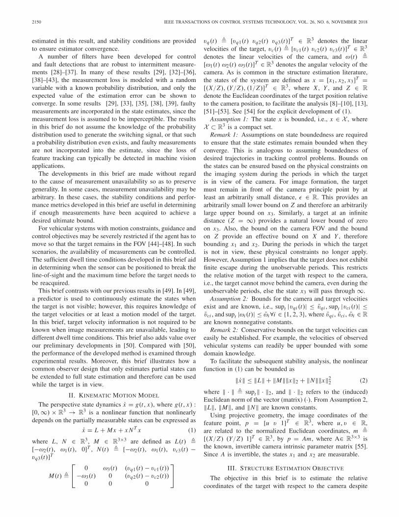
Fig. 3. Evolution of the estimation error for measurement unavailabilitydwell times of 0.5–2.5 s. Each plot shows three experiments for the listeddwell time.

A number of experiments were performed with �t OFFn rang-

ing from 0.5 to 2.5 s, in increments of 0.5 s. Duringthese experiments, �t ON

n was held constant at 4 s, and theTurtlebot was sent constant forward and angular velocitycommands of 0.4 m/s and 0.7 rad/s, respectively, resultingin an approximately circular path. For these target velocities,conditions (6) and (8) dictate that �t OFF

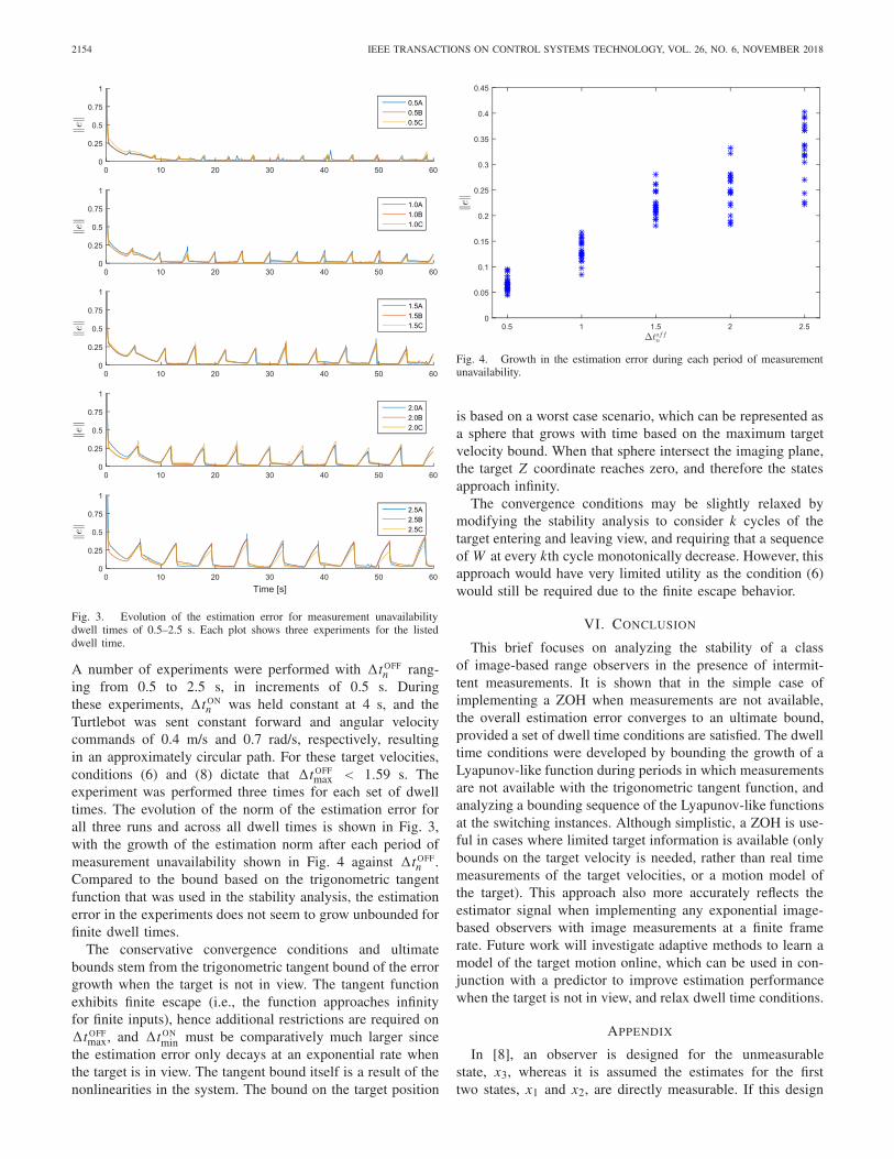
max < 1.59 s. Theexperiment was performed three times for each set of dwelltimes. The evolution of the norm of the estimation error forall three runs and across all dwell times is shown in Fig. 3,with the growth of the estimation norm after each period ofmeasurement unavailability shown in Fig. 4 against �t OFF

n .Compared to the bound based on the trigonometric tangentfunction that was used in the stability analysis, the estimationerror in the experiments does not seem to grow unbounded forfinite dwell times.

The conservative convergence conditions and ultimatebounds stem from the trigonometric tangent bound of the errorgrowth when the target is not in view. The tangent functionexhibits finite escape (i.e., the function approaches infinityfor finite inputs), hence additional restrictions are required on�t OFF

max, and �t ONmin must be comparatively much larger since

the estimation error only decays at an exponential rate whenthe target is in view. The tangent bound itself is a result of thenonlinearities in the system. The bound on the target position

Fig. 4. Growth in the estimation error during each period of measurementunavailability.

is based on a worst case scenario, which can be represented asa sphere that grows with time based on the maximum targetvelocity bound. When that sphere intersect the imaging plane,the target Z coordinate reaches zero, and therefore the statesapproach infinity.

The convergence conditions may be slightly relaxed bymodifying the stability analysis to consider k cycles of thetarget entering and leaving view, and requiring that a sequenceof W at every kth cycle monotonically decrease. However, thisapproach would have very limited utility as the condition (6)would still be required due to the finite escape behavior.

VI. CONCLUSION

This brief focuses on analyzing the stability of a classof image-based range observers in the presence of intermit-tent measurements. It is shown that in the simple case ofimplementing a ZOH when measurements are not available,the overall estimation error converges to an ultimate bound,provided a set of dwell time conditions are satisfied. The dwelltime conditions were developed by bounding the growth of aLyapunov-like function during periods in which measurementsare not available with the trigonometric tangent function, andanalyzing a bounding sequence of the Lyapunov-like functionsat the switching instances. Although simplistic, a ZOH is use-ful in cases where limited target information is available (onlybounds on the target velocity is needed, rather than real timemeasurements of the target velocities, or a motion model ofthe target). This approach also more accurately reflects theestimator signal when implementing any exponential image-based observers with image measurements at a finite framerate. Future work will investigate adaptive methods to learn amodel of the target motion online, which can be used in con-junction with a predictor to improve estimation performancewhen the target is not in view, and relax dwell time conditions.

APPENDIX

In [8], an observer is designed for the unmeasurablestate, x3, whereas it is assumed the estimates for the firsttwo states, x1 and x2, are directly measurable. If this design

PARIKH et al.: SWITCHED SYSTEMS APPROACH TO IMAGE-BASED LOCALIZATION OF TARGETS 2155

were directly implemented, the state estimates may discontin-uously jump whenever the target comes into view, violatingthe continuity assumption of Theorem 1. By using filteredmeasurements for the complete state estimate, the continuityassumption can be satisfied. The observer used in the exper-iments described in Section V is a modified version of theobserver in [8] and is defined by the update laws

˙x1 = h1 x3 + p1 + k1e1˙x2 = h2 x3 + p2 + k2e2

˙x3 = −b3x23 + (x1ω2 − x2ω1)x3 − k3

(h2

1 + h22

)x3

+ k3h1(x1 − p1) + k3h2(x2 − p2) + h1e1 + h2e2

where the error signals, e � [e1 e2 e3]T ∈ R3, are defined as

e � x − x , the velocity signal is defined as b � vq − vc ∈ R3,

k1, k2, k3 ∈ R are positive constants, and the auxiliary signalsh1, h2, p1, p2 ∈ R are defined as in [8]. Using the Lyapunovfunction candidate V = (1/2)e2

1 + (1/2)e22 + (1/2)e2

3 it canbe shown that V ≤ −k1e2

1 − k2e22 − k4e2

3 for some positiveconstant k4 ∈ R, using the same bounding arguments andgain conditions as in [8]. Thus, the augmented observer isexponentially convergent.

ACKNOWLEDGMENT

Any opinions, findings and conclusions or recommendationsexpressed in this material are those of the author(s) and do notnecessarily reflect the views of the sponsoring agency.

REFERENCES

[1] S. Ullman, “The interpretation of structure from motion,” Proc. Roy.Soc. London B, Biol. Sci., vol. 203, no. 1153, pp. 405–426, Jan. 1979.

[2] R. Spica, P. R. Giordano, and F. Chaumette, “Active structure frommotion: Application to point, sphere, and cylinder,” IEEE Trans. Robot.,vol. 30, no. 6, pp. 1499–1513, Dec. 2014.

[3] A. Martinelli, “Vision and IMU data fusion: Closed-form solutions forattitude, speed, absolute scale, and bias determination,” IEEE Trans.Robot., vol. 28, no. 1, pp. 44–60, Feb. 2012.

[4] D. Braganza, D. M. Dawson, and T. Hughes, “Euclidean position estima-tion of static features using a moving camera with known velocities,” inProc. IEEE Conf. Decision Control, New Orleans, LA, USA, Dec. 2007,pp. 2695–2700.

[5] O. Dahl, Y. Wang, A. F. Lynch, and A. Heyden, “Observer formsfor perspective systems,” Automatica, vol. 46, no. 11, pp. 1829–1834,Nov. 2010.

[6] N. Zarrouati, E. Aldea, and P. Rouchon, “So(3)-invariant asymptoticobservers for dense depth field estimation based on visual data andknown camera motion,” in Proc. Amer. Control Conf., Montreal, QC,Canada, Jun. 2012, pp. 4116–4123.

[7] A. Chiuso, P. Favaro, H. Jin, and S. Soatto, “Structure from motioncausally integrated over time,” IEEE Trans. Pattern Anal. Mach. Intell.,vol. 24, no. 4, pp. 523–535, Apr. 2002.

[8] A. P. Dani, N. R. Fischer, Z. Kan, and W. E. Dixon, “Globally exponen-tially stable observer for vision-based range estimation,” Mechatronics,vol. 22, no. 4, pp. 381–389, Jun. 2012.

[9] D. Karagiannis and A. Astolfi, “A new solution to the problem ofrange identification in perspective vision systems,” IEEE Trans. Autom.Control, vol. 50, no. 12, pp. 2074–2077, Dec. 2005.

[10] X. Chen and H. Kano, “A new state observer for perspective systems,”IEEE Trans. Autom. Control, vol. 47, no. 4, pp. 658–663, Apr. 2002.

[11] L. Ma, C. Cao, N. Hovakimyan, C. Woolsey, and W. E. Dixon, “Fastestimation for range identification in the presence of unknown motionparameters,” IMA J. Appl. Math., vol. 75, no. 2, pp. 165–189, 2010.

[12] G. Hu, D. Aiken, S. Gupta, and W. E. Dixon, “Lyapunov-basedrange identification for a paracatadioptric system,” IEEE Trans. Autom.Control, vol. 53, no. 7, pp. 1775–1781, Aug. 2008.

[13] W. E. Dixon, Y. Fang, D. M. Dawson, and T. J. Flynn, “Range iden-tification for perspective vision systems,” IEEE Trans. Autom. Control,vol. 48, no. 12, pp. 2232–2238, Dec. 2003.

[14] X. Chen and H. Kano, “State observer for a class of nonlinear systemsand its application to machine vision,” IEEE Trans. Autom. Control,vol. 49, no. 11, pp. 2085–2091, Nov. 2004.

[15] A. P. Dani, Z. Kan, N. R. Fischer, and W. E. Dixon, “Structure andmotion estimation of a moving object using a moving camera,” in Proc.Amer. Control Conf., Baltimore, MD, USA, 2010, pp. 6962–6967.

[16] A. P. Dani, Z. Kan, N. R. Fischer, and W. E. Dixon, “Structure estimationof a moving object using a moving camera: An unknown input observerapproach,” in Proc. IEEE Conf. Decision Control, Orlando, FL, USA,Dec. 2011, pp. 5005–5012.

[17] D. Liberzon, Switching in Systems and Control. Basel, Switzerland:Birkhüuser Verlag, 2003.

[18] G. Zhai, B. Hu, K. Yasuda, and A. N. Michel, “Stability analysis ofswitched systems with stable and unstable subsystems: An averagedwell time approach,” Int. J. Syst. Sci., vol. 32, no. 8, pp. 1055–1061,Nov. 2001.

[19] M. A. Müller and D. Liberzon, “Input/output-to-state stability and state-norm estimators for switched nonlinear systems,” Automatica, vol. 48,no. 9, pp. 2029–2039, 2012.

[20] M. Sznaier and O. Camps, “Motion prediction for continued autonomy,”in Encyclopedia of Complexity and Systems Science. New York, NY,USA: Springer, 2009, pp. 5702–5718.

[21] M. Sznaier, O. Camps, N. Ozay, T. Ding, G. Tadmor, and D. Brooks,“The role of dynamics in extracting information sparsely encoded inhigh dimensional data streams,” in Dynamics of Information Systems,vol. 40. New York, NY, USA: Springer, 2010, pp. 1–27.

[22] F. Xiong, O. I. Camps, and M. Sznaier, “Dynamic context for trackingbehind occlusions,” in Proc. Eur. Conf. Comput. Vis., Florence, Italy,Oct. 2012, pp. 580–593.

[23] T. Ding, M. Sznaier, and O. Camps, “Receding horizon rank minimiza-tion based estimation with applications to visual tracking,” in Proc. IEEEConf. Decis. Control, Cancun, Mexico, Dec. 2008, pp. 3446–3451.

[24] M. Ayazoglu, B. Li, C. Dicle, M. Sznaier, and O. I. Camps, “Dynamicsubspace-based coordinated multicamera tracking,” in Proc. IEEE Int.Conf. Comput. Vis., Barcelona, Spain, Nov. 2011, pp. 2462–2469.

[25] M. Yang, Y. Wu, and G. Hua, “Context-aware visual tracking,” IEEETrans. Pattern Anal. Mach. Intell., vol. 31, no. 7, pp. 1195–1209,Jul. 2009.

[26] H. Grabner, J. Matas, L. van Gool, and P. Cattin, “Tracking the invisible:Learning where the object might be,” in Proc. IEEE Conf. Comput. Vis.Pattern Recognit., San Francisco, CA, USA, Jun. 2010, pp. 1285–1292.

[27] L. Cerman, J. Matas, and V. Hlavác, “Sputnik tracker: Having acompanion improves robustness of the tracker,” in Proc. Scandin. Conf.Image Anal., Oslo, Norway, Jun. 2009, pp. 291–300.

[28] J. Hu, Z. Wang, H. Gao, and L. K. Stergioulas, “Extended Kalman filter-ing with stochastic nonlinearities and multiple missing measurements,”Automatica, vol. 48, no. 9, pp. 2007–2015, Sep. 2012.

[29] Z. Wang, B. Shen, and X. Liu, “H∞ filtering with randomly occurringsensor saturations and missing measurements,” Automatica, vol. 48,no. 3, pp. 556–562, Mar. 2012.

[30] S. Dey, A. S. Leong, and J. S. Evans, “Kalman filtering with fadedmeasurements,” Automatica, vol. 45, no. 10, pp. 2223–2233, Oct. 2009.

[31] B. Sinopoli, L. Schenato, M. Franceschetti, K. Poolla, M. I. Jordan, andS. S. Sastry, “Kalman filtering with intermittent observations,” IEEETrans. Autom. Control, vol. 49, no. 9, pp. 1453–1464, Sep. 2004.

[32] K. You, M. Fu, and L. Xie, “Mean square stability for Kalmanfiltering with Markovian packet losses,” Automatica, vol. 47, no. 12,pp. 2647–2657, Dec. 2011.

[33] H. Zhang and Y. Shi, “Observer-based H∞ feedback control for arbitrar-ily time-varying discrete-time systems with intermittent measurementsand input constraints,” J. Dyn. Syst., Meas., Control, vol. 134, no. 6,Sep. 2012.

[34] B. Shen, Z. Wang, H. Shu, and G. Wei, “On nonlinear H∞ filteringfor discrete-time stochastic systems with missing measurements,” IEEETrans. Autom. Control, vol. 53, no. 9, pp. 2170–2180, Oct. 2008.

[35] S. C. Smith and P. Seiler, “Optimal pseudo-steady-state estimators forsystems with Markovian intermittent measurements,” in Proc. Amer.Control Conf., vol. 4. 2002, pp. 3021–3027.

[36] H. M. Faridani, “Performance of kalman filter with missing measure-ments,” Automatica, vol. 22, no. 1, pp. 117–120, 1986.

[37] L. K. Carvalho, J. C. Basilio, and M. V. Moreira, “Robust diagnosisof discrete event systems against intermittent loss of observations,”Automatica, vol. 48, no. 9, pp. 2068–2078, 2012.

2156 IEEE TRANSACTIONS ON CONTROL SYSTEMS TECHNOLOGY, VOL. 26, NO. 6, NOVEMBER 2018

[38] F. O. Hounkpevi and E. E. Yaz, “Robust minimum variance linear stateestimators for multiple sensors with different failure rates,” Automatica,vol. 43, no. 7, pp. 1274–1280, 2007.

[39] H. Liang and T. Zhou, “Robust state estimation for uncertain discrete-time stochastic systems with missing measurements,” Automatica,vol. 47, no. 7, pp. 1520–1524, 2011.

[40] J. Liang, Z. Wang, and X. Liu, “State estimation for coupled uncer-tain stochastic networks with missing measurements and time-varyingdelays: The discrete-time case,” IEEE Trans. Neural Netw., vol. 20, no. 5,pp. 781–793, May 2009.

[41] S. Kluge, K. Reif, and M. Brokate, “Stochastic stability of the extendedKalman filter with intermittent observations,” IEEE Trans. Autom.Control, vol. 55, no. 2, pp. 514–518, Feb. 2010.

[42] L. Li and Y. Xia, “Stochastic stability of the unscented Kalman filterwith intermittent observations,” Automatica, vol. 48, no. 5, pp. 978–981,2012.

[43] S. Deshmukh, B. Natarajan, and A. Pahwa, “Stochastic state estimationfor smart grids in the presence of intermittent measurements,” in Proc.IEEE Latin-Amer. Conf. Commun., Nov. 2012, pp. 1–6.

[44] N. R. Gans and S. A. Hutchinson, “A stable vision-based controlscheme for nonholonomic vehicles to keep a landmark in the field ofview,” in Proc. IEEE Int. Conf. Robot. Autom., Roma, Italy, Apr. 2007,pp. 2196–2201.

[45] S. Bhattacharya, R. Murrieta-Cid, and S. Hutchinson, “Optimal pathsfor landmark-based navigation by differential-drive vehicles with field-of-view constraints,” IEEE Trans. Robot., vol. 23, no. 1, pp. 47–59,Feb. 2007.

[46] G. López-Nicolás, N. R. Gans, S. Bhattacharya, C. Sagüés,J. J. Guerrero, and S. Hutchinson, “Homography-based control schemefor mobile robots with nonholonomic and field-of-view constraints,”IEEE Trans. Syst., Man, Cybern. B, Cybern., vol. 40, no. 4,pp. 1115–1127, Aug. 2010.

[47] P. Salaris, D. Fontanelli, L. Pallottino, and A. Bicchi, “Shortest paths fora robot with nonholonomic and field-of-view constraints,” IEEE Trans.Robot., vol. 26, no. 2, pp. 269–281, Apr. 2010.

[48] L. R. G. Carrillo, G. R. Flores Colunga, G. Sanahuja, and R. Lozano,“Quad rotorcraft switching control: An application for the task ofpath following,” IEEE Trans. Control Syst. Technol., vol. 22, no. 4,pp. 1255–1267, Jul. 2014.

[49] A. Parikh, T.-H. Cheng, and W. E. Dixon, “A switched systems approachto vision-based localization of a target with intermittent measurements,”in Proc. Amer. Control Conf., Jul. 2015, pp. 4443–4448.

[50] A. Parikh, T.-H. Cheng, R. Licitra, and W. E. Dixon, “A switchedsystems approach to image-based localization of targets that temporarilyleave the field of view,” in Proc. IEEE 53rd Annu. Conf. DecisionControl, Dec. 2014, pp. 2185–2190.

[51] J. Civera, A. J. Davison, and J. M. M. Montiel, “Inverse depth para-metrization for monocular SLAM,” IEEE Trans. Robot., vol. 24, no. 5,pp. 932–945, Oct. 2008.

[52] B. Ghosh, M. Jankovic, and Y. Wu, “Perspective problems in systemtheory and its application to machine vision,” J. Math. Syst. Estim.Control, vol. 4, no. 1, pp. 3–38, 1994.

[53] R. Abdursul, H. Inaba, and B. K. Ghosh, “Nonlinear observers forperspective time-invariant linear systems,” Automatica, vol. 40, no. 3,pp. 481–490, Mar. 2004.

[54] F. Chaumette and S. Hutchinson, “Visual servo control. I. Basicapproaches,” IEEE Robot. Autom. Mag., vol. 13, no. 4, pp. 82–90,Dec. 2006.

[55] Y. Ma, S. Soatto, J. Kosecka, and S. Sastry, An Invitation to 3-D Vision.New York, NY, USA: Springer, 2004.

[56] A. De Luca, G. Oriolo, and P. R. Giordano, “Feature depth observationfor image-based visual servoing: Theory and experiments,” Int. J. Robot.Res., vol. 27, no. 10, pp. 1093–1116, Oct. 2008.

[57] F. Morbidi and D. Prattichizzo, “Range estimation from a movingcamera: An immersion and invariance approach,” in Proc. IEEE Int.Conf. Robot. Autom., Kobe, Japan, May 2009, pp. 2810–2815.

[58] H. K. Khalil, Nonlinear Systems, 3rd ed. Upper Saddle River, NJ, USA:Prentice-Hall, 2002.

[59] W. Rudin, Principles of Mathematical Analysis. New York, NY, USA:McGraw-Hill, 1976.

[60] S. S. Mehta, T. Burks, and W. E. Dixon, “Vision-based localization ofa wheeled mobile robot for greenhouse applications: A daisy-chainingapproach,” Comput. Electron. Agricult., vol. 63, no. 1, pp. 28–37, 2008.

[61] K. Dupree, N. R. Gans, W. MacKunis, and W. E. Dixon, “Euclideancalculation of feature points of a rotating satellite: A daisy-chainingapproach,” AIAA J. Guid. Control Dyn., vol. 31, no. 4, pp. 954–961,2008.

[62] R. Sharma, S. Quebe, R. W. Beard, and C. N. Taylor, “Bearing-onlycooperative localization,” J. Intell. Robot. Syst., vol. 72, nos. 3–4,pp. 429–440, Dec. 2013.

[63] S. I. Roumeliotis and G. A. Bekey, “Distributed multirobot localization,”IEEE Trans. Robot. Autom., vol. 18, no. 5, pp. 781–795, Oct. 2002.

[64] A. I. Mourikis and S. I. Roumeliotis, “Performance analysis of mul-tirobot Cooperative localization,” IEEE Trans. Robot., vol. 22, no. 4,pp. 666–681, Aug. 2006.

[65] X. S. Zhou and S. I. Roumeliotis, “Robot-to-robot relative pose esti-mation from range measurements,” IEEE Trans. Robot., vol. 24, no. 6,pp. 1379–1393, Dec. 2008.

[66] S. Garrido-Jurado, R. Muñoz-Salinas, F. J. Madrid-Cuevas, andM. J. Marín-Jiménez, “Automatic generation and detection of highlyreliable fiducial markers under occlusion,” Pattern Recognit., vol. 47,no. 6, pp. 2280–2292, 2014.