optimal control of switched-input and uncertain systems
TRANSCRIPT

Research Collection
Doctoral Thesis
Optimal control of switched-input and uncertain systems
Author(s): Nolde, Kristian
Publication Date: 2008
Permanent Link: https://doi.org/10.3929/ethz-a-005680020
Rights / License: In Copyright - Non-Commercial Use Permitted
This page was generated automatically upon download from the ETH Zurich Research Collection. For moreinformation please consult the Terms of use.
ETH Library

Diss. ETH No. 17886
Optimal Control of Switched-input andUncertain Systems
A dissertation submitted to the
SWISS FEDERAL INSTITUTE OF TECHNOLOGY
ZURICH
for the degree of
Doctor of Sciences
presented by
KRISTIAN NOLDE
Dipl.-Ing, TU Hamburg-Harburg
born March 1, 1977
citizen of Hamburg, Germany
accepted on the recommendation of
Prof. Dr. Manfred Morari, examiner
Prof. Dr. Rüdiger Schultz, co-examiner
2008

c©2008 Kristian NoldeAll Rights reserved


To my family ...


Abstract
The thesis is concerned with three application projects that deal with optimal controlof switched-input and uncertain systems. In switched-input systems some or all ofthe system inputs take binary values. In uncertain systems the dynamics or theoutput are affected by random parameters. In the thesis it is shown how to effectivelycompute optimal control inputs for switched-input and uncertain systems.
In order to show this, an application-driven approach is taken. In this approachoptimal controllers for switched-input and/or uncertain systems from different ap-plications are designed. The projects are presented in three parts of the thesis:
In the first part the development of an optimal controller for thermal printheadsis presented. A first-order linear system with a non-linear output mapping con-taining stochastic noise is proposed as a model for the printing dynamics. Themodel parameters are identified and an optimal control problem is formulated todetermine the printhead input. The control algorithm is successfully tested on astandard thermal printer. A sensitivity analysis is performed using simulations andexperiments in order to analyze the printing quality on varying setups with differentprintheads, printing media and ribbons. A tuning strategy is derived to adapt tochanging setups without having to recompute the optimization problem. Robust-ness of the resulting controller is shown in experiments. Comparing the proposedcontroller to a current control implementation shows a significant quality gain inbarcode readability (ISO/IEC 15416).
The second part presents two load tracking scheduling problem. The first prob-lem deals with the scheduling of employees so that the employee presence tracks apre-specified demand curve. Requirements such as minimum employee presence orconstraints on the shift length have to be respected. The second problem is con-cerned with the energy-cost optimal scheduling of a steel plant. In the steel plantthe total electrical load generated by all machines must track a pre-specified energycurve as close as possible, while respecting constraints that arise from production.For both problems a comparison of discrete-time and continuous-time models of thescheduling problems is made. The results show that in the workforce planning a so-lution is computed faster for the discrete-time model. In the steel plant schedulingthe continuous-time model is superior. It is argued that discrete-time models are
ix

x
superior for problems where only few possible switching time points exist, i. e. timepoints when tasks can start or end. Continuous-time formulations do not seem re-stricted by the number of possible time points, but their limitation appears to be inthe number of possible arrangements of the tasks that are to be scheduled. Also, weshow an example for the continuous-time problem where small parameter changeslead to large changes in the computation time.
The third part is concerned with the medium term control of a hydro-thermalsystem. In this project a multistage stochastic programming formulation is presentedfor monthly production planning of the system. Stochasticity from variations inwater reservoir inflows and fluctuations in demand of electric energy are consideredexplicitly. The problem can be solved efficiently via Nested Benders Decomposition.The solution is implemented in a model predictive control setup, and performanceof this control technique is demonstrated in simulations. Tuning parameters such asprediction horizon and shape of the stochastic programming tree are identified andtheir effects are analyzed.
In the conclusion of the thesis the results of the different projects are related toeach other. Three different approaches that were successful in computing input sig-nals for switched-input systems are summarized. The conclusion also combines thedifferent concepts that were used for treating uncertainty in the systems. Observa-tions on the computational complexity of the application projects are given.

Zusammenfassung
In der vorliegenden Arbeit werden drei Anwendungsprojekte behandelt, die sich mitder optimalen Steuerung von Systemen mit geschalteten Eingängen und Unsicher-heiten beschäftigen. In Systemen mit geschalteten Eingängen besitzen einige oderalle der Systemeingänge Binärwerte. In unsicheren Systemen ist die Systemdynamikoder das Ausgangssignal durch zufällige Parameter beeinflusst. In der Arbeit wirdgezeigt, wie optimale Steuersignale für Systeme mit geschalteten Eingängen undUnsicherheiten effizient berechnet werden können.
Die Arbeit verfolgt dazu einen anwendungsorientierten Ansatz. In diesem Ansatzwird in mehreren Anwendungsprojekten für Systeme mit geschalteten Eingängenund/oder Unsicherheit eine optimale Steuerung oder Regelung entworfen. Die Pro-jekte sind auf drei Abschnitte der Arbeit aufgeteilt:
Im ersten Abschnitt wird die Entwicklung einer optimalen Steuerung für ther-mische Druckköpfe vorgestellt. Die Temperaturdynamik im Druckkopf wird dazumit einem linearen Modell erster Ordnung approximiert. Die Druckausgabe wird alsnichtlineare Funktion der Temperatur angegeben. Die Druckausgabe ist mit einerstochastischen Unsicherheit behaftet. Es werden die Modellparameter identifiziertund ein Optimalregelungsproblem wird aufgestellt. Mit Hilfe des Optimalreglerswerden die Eingangssignale für den Druckkopf bestimmt. Der erfolgreiche Test desOptimalreglers auf einem typischen Thermodrucker wird gezeigt. Um die Änderun-gen der Druckqualität in unterschiedlichen Konfigurationen, z.B. variierende Druck-köpfe, Druck-Medien und Farbbänder, zu analysieren wird eine Sensitivitätsanalysemittels Experimenten und Simulationen durchgeführt. Aus deren Ergebnissen wirdeine Tuning-Strategie abgeleitet. Die Tuning Strategie erlaubt die Anpassung desDruckers an neue Konfigurationen, ohne dass ein neues Optimierungsproblem gelöstwerden muss. Robustheit des resultierenden Reglers wird in Experimenten gezeigt.Im Vergleich des vorgeschlagenen Reglers zu einer bestehenden Implementierungzeigt sich ein signifikanter Qualitätsgewinn beim Erkennen gedruckter Barcodes (ISO/ IEC 15416).
Der zweite Abschnitt der Dissertation beschäftigt sich mit zwei Bedarfsfolge-planungsproblemen. Das erste Problem befasst sich mit der bedarfsgerechten Ein-satzplanung von Mitarbeitern. Deren Einsätze sollen so geplant werden, dass die
xi

xii
Mitarbeiterpräsenz einer im Voraus festgelegten Nachfrage-Kurve folgt. Anforder-ungen wie eine Minimalpräsenz von Mitarbeitern oder Beschränkungen von derenSchichtlänge müssen in der Planung berücksichtigt werden. Das zweite Problembetrifft die energiekostenoptimale Produktionsplanung in einem Stahlwerk. In demStahlwerk soll dazu die von alle Maschinen zusammen generierte elektrische Lasteiner im Voraus festgelegten Lastkurve folgen. Die Einsatzpläne der Maschinenmüssen dabei alle Nebenbedingungen in der Produktion berücksichtigen. Die Summeihrer Energieverbräuche soll weder eine Über- noch eine Unterdeckung der Vorgabeergeben. Für einen Vergleich werden für die beiden Planungsprobleme jeweils miteinem auf kontinuierlicher Zeit und einem auf Zeitdiskretisierung basierendes Plan-ungsmodell beschrieben. Für beide Probleme werden das zeitkontinuierliche unddas zeitdiskrete Modell implementiert und getestet. Die Ergebnisse zeigen, dasssich im Fall des Mitarbeitereinsatzplanungsproblem mit einem zeitdiskretem Modelldie optimale Planung schneller errechnen lässt. Im Planungsproblem für das Stahl-werk ist das zeitkontinuierliche Modell in der Berechnung eines Produktionsplansüberlegen. Es wird argumentiert, dass zeitdiskrete Modelle für Probleme überlegensind, die nur wenige mögliche Schaltzeitpunkte, sprich Zeitpunkte an denen Auf-gaben oder Schichten beginnen und enden, beinhalten. Formulierungen mit kon-tinuierlichen Zeitvariablen besitzen diese Einschränkung nicht, allerdings werdendiese durch die Anzahl der Anordnungen von Aufgaben eingeschränkt. Wird dieseAnzahl von Anordnungen zu gross, dann lassen sich die Probleme nicht mehr inangemessener Zeit lösen.
Der dritte Abschnitt befasst sich mit der Mittelfristplanung eines Hydrother-mischen Kraftwerkssystem. In ihm wird eine Multistage-Stochastic-ProgrammingFormulierung zur Lösung eines monatlichen Produktionsplanungsproblems für einhydrothermisches Kraftwerkssystem vorgestellt. Diese Modellierung beinhaltet ex-plizit die stochastischen Variationen der Zuflüsse zu den Wasserspeichern, sowie dieSchwankungen des elektrischen Energiebedarfs. Das Problem wird unter Anwendungder Nested Benders Decomposition effizient gelöst. Simulationen des geschlossenenRegelkreises werden vorgestellt, um die Funktionsweise des Reglers zu zeigen. DieLösungen des Problems für mittlere Zeithorizonte können als Eingangssignale fürRegler mit kurzen Zeithorizonten genutzt werden. Somit wird ein Aufbrauchen desgespeicherten Wassers durch zu kurze Planungshorizonte vermieden.
In den Schlussfolgerungen der Dissertation werden die Ergebnisse der verschiede-nen Projekte zusammengefasst. Drei in den Anwendungsprojekten erfolgreiche An-sätze zur Berechnung der Signale für eingangsgeschaltete Systeme werden vorgestellt.Desweiteren werden die in der Arbeit genutzten Konzepte zur Steuerungs- undReglerauslegung für Systeme unter Unsicherheit vorgestellt. Es werden Beobacht-

xiii
ungen über die Rechenkomplexität der Projekte zusammengefasst.


Acknowledgments
Finishing a PhD in engineering is a complex venture and I would have had no chanceof success, if it was not for many people who supported, helped and encouraged me.I owe my sincere gratitude to all of them.
I would like to thank Prof. Morari who accepted me as a student and got mestarted on a number of exciting application problems. I would like to thank him forhis encouragement to explore fields outside the immediate focus of our lab. He alsohas greatly supported me to take the first steps into entrepreneurship and therebyallowed me to gain much more experience in the business world. I am very thankfulfor all the flexibility that I was given.
I would also like to thank two more professors Ignacio Grossmann and RüdigerSchultz. Both have been very influential on my work and their input has been ofgreat help and is highly appreciated. Moreover, it has been a great pleasure knowingthem. Pablo Parrilo and Robert Riener were assistant professors during my time atIfA and I very much enjoyed all interactions with both of them.
Of course I would like to thank my PhD colleagues, especially my office matesUrban and Frauke. You are great! It has been a lot of fun to share so many greatmoments, ideas and discussions. I very much hope that we will stay in touch. Ialso want to thank Dominik for a good company in the office during my first yearsat ETH. Furthermore, many thanks go to Heli and Philipp for being fantastic nextdoor office neighbors (actually we are only separated by a very thin wall and I canhear you talking right now).
I am indebted to many current and past members of IfA who helped in many waysand made IfA a great place to work at. This includes my present PhD colleagues:Miroslav, Thomas, Antonello, Kimberly, George, Ioannis F., Cristian, Michael K.,Kostas, Andreas, Marc, Ioannis L., Andreas, Robert, Alexander, Alessandra, Stefan,Akin, Sean, Ningbo and Melanie. I wish all of them good success with their researchand thesis work. My gratitude also goes to all the postdocs, many of whom alreadyleft IfA to continue their careers: Mato, Giovanni, Eleonora B., Marta, Debasish,Vaclav, Eugenio, Frank, Eva, Gültekin, Mirko, Tobias G., Pascal, Franta, Thierry,Michal, Sébastien, Rainer, Tobias N., Bundit, Georgios P., Vale and Ele. It has beengreat to get to know them and work together.
xv

xvi
IfA would not be complete if it was not for the secretarial staff: Danielle, Esther,Gabi, Martha, Alice and Martine. Besides keeping everything running they alsogreatly contributed to the pleasant atmosphere at the lab.
The work in this thesis would not have been possible if it was not for the industrialpartners who sponsored and supported my research: Asea Brown Boveri Ltd, ApexOptimization GmbH, Avery Dennison Deutschland GmbH and Rohm Ltd.
I would like to thank my semester and diploma students, especially Markus andChristian, for their good work. Many of their ideas found their way into this thesis.I also owe many credits to Raphael for his careful work on the experiments withinthe thermal printing project; his work has been a great help and it was very niceworking together. I would like to thank my colleague and business partner Colin, ithas been great fun starting a company together. I hope we make it grow ... or atleast get rich!
Of course life does not only take place in the lab and many friends in Zurich andall over the world were great company and support during my PhD time.
In particular, I would like to thank Natalia for proof reading and everything elseshe did! Last but not least I would like to thank my parents and my brother forbeing a great family and helping me to accomplish all the smaller and bigger goalsso far.


Contents
1 Introduction 1
Bibliography . . . . . . . . . . . . . . . . . . . . . . . . . . . . . . . . 10
I Thermal Printhead Control 15
2 Thermal Printhead Control 17
2.1 Introduction . . . . . . . . . . . . . . . . . . . . . . . . . . . . . . . . 172.2 Model of Printing Process . . . . . . . . . . . . . . . . . . . . . . . . 19
2.2.1 Printhead Model . . . . . . . . . . . . . . . . . . . . . . . . . 192.2.2 Identification of the Model Parameters . . . . . . . . . . . . . 22
2.3 Controller Design . . . . . . . . . . . . . . . . . . . . . . . . . . . . . 252.3.1 Optimal Controller . . . . . . . . . . . . . . . . . . . . . . . . 252.3.2 Lookup Table Controller . . . . . . . . . . . . . . . . . . . . . 262.3.3 Tuning Rule . . . . . . . . . . . . . . . . . . . . . . . . . . . . 27
2.3.3.1 Lookup tables for a set of setups . . . . . . . . . . . 282.3.3.2 Lookup Table Selection via Test Pattern . . . . . . . 29
2.4 Experimental Results . . . . . . . . . . . . . . . . . . . . . . . . . . . 302.4.1 Identification and Optimal Controller Design . . . . . . . . . . 302.4.2 Tuning Rule . . . . . . . . . . . . . . . . . . . . . . . . . . . . 342.4.3 Results . . . . . . . . . . . . . . . . . . . . . . . . . . . . . . . 46
2.5 Conclusions . . . . . . . . . . . . . . . . . . . . . . . . . . . . . . . . 46Bibliography . . . . . . . . . . . . . . . . . . . . . . . . . . . . . . . . 49
II Load Tracking Scheduling 53
3 Load Tracking Scheduling 55
3.1 Introduction . . . . . . . . . . . . . . . . . . . . . . . . . . . . . . . . 553.2 Models for scheduling problems . . . . . . . . . . . . . . . . . . . . . 57
3.2.1 Discrete Time Models . . . . . . . . . . . . . . . . . . . . . . 58
xix

xx Contents
3.2.1.1 General Discrete Time Scheduling Models . . . . . . 593.2.1.2 Mixed Logic Dynamical Models . . . . . . . . . . . . 59
3.2.2 Continuous Time Models . . . . . . . . . . . . . . . . . . . . . 623.3 Examples of Load Tracking Scheduling Problems . . . . . . . . . . . 63
3.3.1 Employee Scheduling . . . . . . . . . . . . . . . . . . . . . . . 633.3.1.1 Requirements and Objective . . . . . . . . . . . . . . 643.3.1.2 Discrete Time Model . . . . . . . . . . . . . . . . . . 653.3.1.3 Continuous Time Model . . . . . . . . . . . . . . . . 673.3.1.4 Comparison of the Models . . . . . . . . . . . . . . . 70
3.3.2 Steel Manufacturing Problem . . . . . . . . . . . . . . . . . . 793.3.2.1 Objective and Constraints . . . . . . . . . . . . . . . 803.3.2.2 Discrete Time Model . . . . . . . . . . . . . . . . . . 823.3.2.3 Continuous Time . . . . . . . . . . . . . . . . . . . . 873.3.2.4 Comparison of Models and Analysis . . . . . . . . . 92
3.4 Conclusions . . . . . . . . . . . . . . . . . . . . . . . . . . . . . . . . 106Bibliography . . . . . . . . . . . . . . . . . . . . . . . . . . . . . . . . 110
III Hydro-thermal System Control 117
4 Hydro-thermal System Control 119
4.1 Introduction . . . . . . . . . . . . . . . . . . . . . . . . . . . . . . . . 1194.2 System Modeling . . . . . . . . . . . . . . . . . . . . . . . . . . . . . 1214.3 Model Predictive Control . . . . . . . . . . . . . . . . . . . . . . . . . 124
4.3.1 Stochastic optimization problem . . . . . . . . . . . . . . . . . 1244.3.2 Stochastic model predictive control . . . . . . . . . . . . . . . 128
4.4 Simulations . . . . . . . . . . . . . . . . . . . . . . . . . . . . . . . . 1294.4.1 Simulation problem setup . . . . . . . . . . . . . . . . . . . . 1324.4.2 Initial test of the proposed controller . . . . . . . . . . . . . . 1324.4.3 Constant number of paths trees with varying horizon length . 1344.4.4 Constant number of child nodes trees with varying horizon
length . . . . . . . . . . . . . . . . . . . . . . . . . . . . . . . 1384.4.5 Constant number of paths trees with varying tree shapes . . . 138
4.5 Conclusions . . . . . . . . . . . . . . . . . . . . . . . . . . . . . . . . 140Bibliography . . . . . . . . . . . . . . . . . . . . . . . . . . . . . . . . 143
5 Conclusion 147
Bibliography . . . . . . . . . . . . . . . . . . . . . . . . . . . . . . . . 155

Contents xxi
6 Outlook 157
Bibliography . . . . . . . . . . . . . . . . . . . . . . . . . . . . . . . . 160


List of Figures
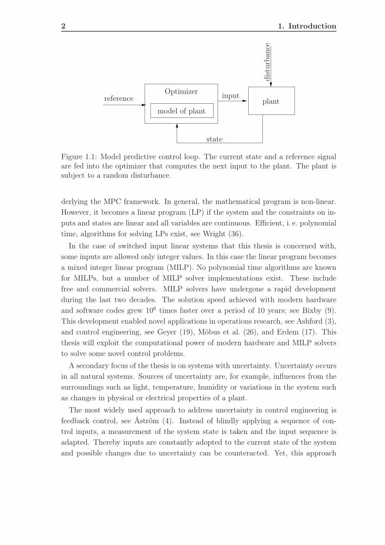
1.1 Model predictive control loop. The current state and a referencesignal are fed into the optimizer that computes the next input to theplant. The plant is subject to a random disturbance. . . . . . . . . . 2
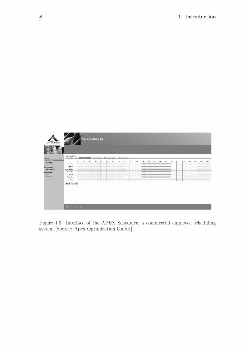
1.2 A thermal printer [Source: Avery Dennison Deutschland GmbH]. . . 61.3 Interface of the APEX Scheduler, a commercial employee scheduling
system [Source: Apex Optimization GmbH]. . . . . . . . . . . . . . . 81.4 The Dalles-Dam Washington, US [Source: United States Geological
Survey]. . . . . . . . . . . . . . . . . . . . . . . . . . . . . . . . . . . 10
2.1 Printhead as an array of resistors, each representing one heat element.The figure shows three heat elements (HE). . . . . . . . . . . . . . . . 19
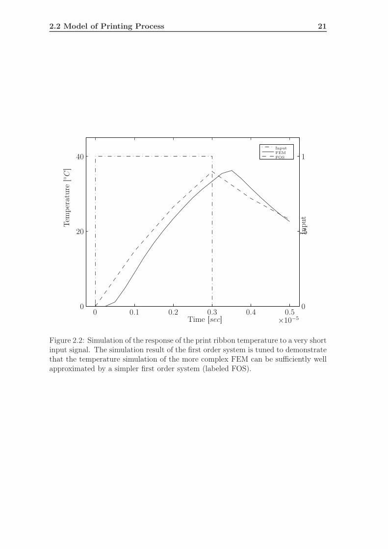
2.2 Simulation of the response of the print ribbon temperature to a veryshort input signal. The simulation result of the first order system istuned to demonstrate that the temperature simulation of the morecomplex FEM can be sufficiently well approximated by a simpler firstorder system (labeled FOS). . . . . . . . . . . . . . . . . . . . . . . . 21
2.3 Geometry of the printhead as used for finite element simulations. . . 232.4 Fraction of on dot profile, generated from a scan of a barcode that is
printed perpendicular to the print medium movement. . . . . . . . . . 242.5 Identification results for the parameters α, β at print speed 4 inch/sec
for medium ribbon combination (indicated by the symbol) and up tofive different printheads. . . . . . . . . . . . . . . . . . . . . . . . . . 31
2.6 Identification results for the parameters α, β at print speed 2 inch/secfor medium ribbon combination (indicated by the symbol) and up tofive different printheads. . . . . . . . . . . . . . . . . . . . . . . . . . 32
2.7 Identification results for the parameters α, β at print speed 6 inch/secfor medium ribbon combination (indicated by the symbol) and up tofive different printheads. . . . . . . . . . . . . . . . . . . . . . . . . . 33
2.8 Comparison of barcodes for current and optimized controller printedat 4 inch/sec. . . . . . . . . . . . . . . . . . . . . . . . . . . . . . . . 35
xxiii

xxiv List of Figures
2.9 Simulation results for printing with a controller designed for a setupmarked with a star on other setups. The lines indicate setups withequal print quality. . . . . . . . . . . . . . . . . . . . . . . . . . . . . 37
2.10 Experimental results for printing with 4 inch per second with a con-troller designed for printing on type-plate material using ribbon B110C(marked with a star) on other setups. Quality is evaluated using ANSIGrades. The lines are used to illustrate where setups with equal printquality might be expected. . . . . . . . . . . . . . . . . . . . . . . . 38
2.11 Experimental results for printing with 4 inch per second with a con-troller designed for printing on sticker using ribbon 2740 (marked witha star) on other setups. Quality is evaluated using ANSI Grades. Thelines are used to illustrate where setups with equal print quality mightbe expected. . . . . . . . . . . . . . . . . . . . . . . . . . . . . . . . 39
2.12 Experimental results for printing with 4 inch per second with a con-troller designed for printing on PVC using ribbon 2560 (marked witha star) on other setups. Quality is evaluated using ANSI Grades.The lines are used to illustrate where setups with equal print qualitymight be expected. . . . . . . . . . . . . . . . . . . . . . . . . . . . . 40
2.13 Experimental results for printing with 2 inch per second on with acontroller designed for a setup marked with a star on other setups.Quality is evaluated using ANSI Grades. The lines are used to illus-trate where setups with equal print quality might be expected. . . . 42
2.14 Experimental results for printing with 2 inch per second with a con-troller designed for printing on (setup marked with a star) on othersetups. Quality is evaluated using ANSI Grades. The lines are usedto illustrate where setups with equal print quality might be expected. 43
2.15 Experimental results for printing with 6 inch per second controllerdesigned for a setup marked with a star on other setups. Quality isevaluated using ANSI Grades. The lines are used to illustrate wheresetups with equal print quality might be expected. . . . . . . . . . . 44
2.16 Experimental results for printing with 6 inch per second a controllerdesigned for a setup marked with a star on other setups. Quality isevaluated using ANSI Grades. The lines are used to illustrate wheresetups with equal print quality might be expected. . . . . . . . . . . 45
2.17 Test pattern for tuning. The percentage of strobe-on pulses betweenthe lines is gradually increased, at some point the printing thresholdis reached and the area in-between blackens. . . . . . . . . . . . . . . 45

List of Figures xxv
3.1 Discrete time solution to employee scheduling problem No. 1. . . . . . 713.2 Continuous time solution to employee scheduling problem No. 1. . . . 723.3 Continuous time solution to employee scheduling problem No. 2. . . . 733.4 Discrete time solution to employee scheduling problem No. 2. . . . . . 743.5 Continuous time solution for scheduling of 5 employees (example No. 3). 763.6 Discrete time solution for scheduling of 5 employees (example No. 3). 773.7 Discrete time solution with a detailed tracking curve for scheduling 5
employees (example No. 4). . . . . . . . . . . . . . . . . . . . . . . . 783.8 Steel plant diagram. . . . . . . . . . . . . . . . . . . . . . . . . . . . 813.9 Illustration of Objective Function. . . . . . . . . . . . . . . . . . . . . 813.10 Six possible classes of load interval overlap. . . . . . . . . . . . . . . 903.11 Discrete time solution of the initial test scheduling problem. . . . . . 943.12 Continuous time solution of the initial scheduling problem. . . . . . . 953.13 Continuous time solution of the realistic test problem. . . . . . . . . . 993.14 Solution with tighter min-/max task durations. . . . . . . . . . . . . 1033.15 Solution with relaxed min-/max task durations. . . . . . . . . . . . . 1043.16 Flexible tasks enlarge the search tree by adding new cases. . . . . . . 1053.17 Sub-optimal solution for a 4 hour schedule. . . . . . . . . . . . . . . . 107
4.1 Example of a simple hydro-thermal system with two hydro-powerplants and one thermal plant. . . . . . . . . . . . . . . . . . . . . . . 122
4.2 Event decision structure of the hydro-thermal system. . . . . . . . . . 1244.3 Event tree example with 4 stages and 18 paths in total. . . . . . . . . 1274.4 Inflow profile of The Dalles dam in Washington/Oregon, USA. . . . . 1314.5 Closed loop simulation result. . . . . . . . . . . . . . . . . . . . . . . 1334.6 Simulations of controllers with approximately constant number of
path in the stochastic program, but different number of time stages(prediction horizon). . . . . . . . . . . . . . . . . . . . . . . . . . . . 135
4.7 Simulation results of controllers with approximately 254 paths, butdifferent number of time stages (prediction horizon). . . . . . . . . . . 137
4.8 Simulations for controllers based on two-child and three-child eventtrees with different number of time stages (prediction horizon). . . . . 139
4.9 Simulations for controllers with constant number of paths and horizonlength 7. The simulations started with four-child trees and ended forskewedness 12 with 16’384 realizations for time stage 1 followed bydeterministic paths to the leaf nodes of the event tree. . . . . . . . . . 141


List of Tables
2.1 Parameter values. . . . . . . . . . . . . . . . . . . . . . . . . . . . . 312.2 Comparison of the ANSI ratings for the barcodes printed on sticker
medium at different speeds on a 300dpi printhead. Modulewidth de-termines the number of dots of the thinnest line in the barcode. ANSIratings range from 0 to 4, with 4 being the best. . . . . . . . . . . . 35
2.3 Matching the results from the test pattern evaluation with the com-puted lookup tables. . . . . . . . . . . . . . . . . . . . . . . . . . . . 42
2.4 Performance evaluation for: Speed 4 inch/sec ·Modulewidth 5 · Print-head# 1(new) . . . . . . . . . . . . . . . . . . . . . . . . . . . . . . . 47
2.5 Performance evaluation for: Speed 4 inch/sec ·Modulewidth 5 · Print-head# 6 (stress tested) . . . . . . . . . . . . . . . . . . . . . . . . . . 47
2.6 Performance evaluation for: Speed 4 inch/sec ·Modulewidth 2 · Print-head# 5 (new, not used during identification experiments) . . . . . . 48
3.1 Logic relations and their conversions into mixed-integer relations. . . 613.2 Model parameters for the employee scheduling problems. . . . . . . . 713.3 Energy consumption. . . . . . . . . . . . . . . . . . . . . . . . . . . . 933.4 Initial test load curve. . . . . . . . . . . . . . . . . . . . . . . . . . . 933.5 Task list for the initial test. . . . . . . . . . . . . . . . . . . . . . . . 963.6 Load curve for the realistic test example. . . . . . . . . . . . . . . . . 973.7 Task list for the realistic test. . . . . . . . . . . . . . . . . . . . . . . 973.8 Task list for parameter variation test with tight min-/max task du-
rations. . . . . . . . . . . . . . . . . . . . . . . . . . . . . . . . . . . . 1003.9 Task list for parameter variation test with relaxed min-/max task
durations. . . . . . . . . . . . . . . . . . . . . . . . . . . . . . . . . . 1013.10 Task list for parameter variation test with tight min-/max task du-
rations. . . . . . . . . . . . . . . . . . . . . . . . . . . . . . . . . . . . 1023.11 Load Curve for a 4 hour scheduling example. . . . . . . . . . . . . . . 1083.12 Task list for 4 hour scheduling test. . . . . . . . . . . . . . . . . . . . 109
4.1 Parameters used for the simulations. . . . . . . . . . . . . . . . . . . 133
xxvii

xxviii List of Tables
4.2 Constant number of path trees. . . . . . . . . . . . . . . . . . . . . . 1354.3 Small constant number of path trees used to compute a large sample. 1364.4 Comparison of controllers with approximately 254 paths, see Table
4.3. Probability of controller no. A being better than controller no. B. 1374.5 Skewed trees. . . . . . . . . . . . . . . . . . . . . . . . . . . . . . . . 141


1 Introduction
Switched input and uncertain systems are an extension of linear systems. Bothproperties, switching and uncertainty, allow the description of a broader class ofproblems than those that are possible by using deterministic linear systems alone.We first discuss linear systems with switching and then introduce models containingstochastic components.
By inclusion of the switching property the systems under consideration now havediscrete and continuous valued parts. Therefore they fall in the class of what socalled hybrid systems.
The field of modeling and control of hybrid systems has recently become veryactive. Hybrid systems not only pose theoretical challenges, but also allow newways to model and control dynamical systems, see Geyer (19) for examples of hybridsystems. Recently, optimal control schemes for hybrid systems have been proposed.The schemes are based on discrete-time constrained finite-time optimal control witha receding horizon policy, often referred to as Model Predictive Control (MPC), seeMaciejowski (23).
In MPC a constrained optimization problem is solved for a finite time horizoninto the future. The decision variables of the optimization problem are the controlinputs for the time horizon. The constraints of the optimization variables are theplant dynamics and limitation on inputs and states. The current state of the plantenters the optimization problem as a parameter. The optimization then yields anoptimal sequence of control inputs that minimizes its objective function.
In receding horizon policy, only the first control input of this sequence is applied.The control sequence gets recomputed at the next sampling instant over a shiftedhorizon. Thereby a feedback is provided and the control loop is closed, see Figure 1.1for an illustration of MPC control loop. The advantage of MPC is its ability tosystematically cope with constraints on manipulated variables, states and outputs.Furthermore, it can address systems with multiple inputs and outputs. MPC hasbeen extensively reviewed in survey papers, for example, Mayne et al. (25) and Qin& Badgwell (30). An introduction to different classes of MPC problems is providedin Camacho & Bordons (11) and Maciejowski (23).
A mathematical program solver is needed to solve the optimization problem un-
1
2 1. Introduction
referenceOptimizer
model of plant
input
state
plant
dist
urba
nce
Figure 1.1: Model predictive control loop. The current state and a reference signalare fed into the optimizer that computes the next input to the plant. The plant issubject to a random disturbance.
derlying the MPC framework. In general, the mathematical program is non-linear.However, it becomes a linear program (LP) if the system and the constraints on in-puts and states are linear and all variables are continuous. Efficient, i. e. polynomialtime, algorithms for solving LPs exist, see Wright (36).
In the case of switched input linear systems that this thesis is concerned with,some inputs are allowed only integer values. In this case the linear program becomesa mixed integer linear program (MILP). No polynomial time algorithms are knownfor MILPs, but a number of MILP solver implementations exist. These includefree and commercial solvers. MILP solvers have undergone a rapid developmentduring the last two decades. The solution speed achieved with modern hardwareand software codes grew 106 times faster over a period of 10 years; see Bixby (9).This development enabled novel applications in operations research, see Ashford (3),and control engineering, see Geyer (19), Möbus et al. (26), and Erdem (17). Thisthesis will exploit the computational power of modern hardware and MILP solversto solve some novel control problems.
A secondary focus of the thesis is on systems with uncertainty. Uncertainty occursin all natural systems. Sources of uncertainty are, for example, influences from thesurroundings such as light, temperature, humidity or variations in the system suchas changes in physical or electrical properties of a plant.
The most widely used approach to address uncertainty in control engineering isfeedback control, see Åström (4). Instead of blindly applying a sequence of con-trol inputs, a measurement of the system state is taken and the input sequence isadapted. Thereby inputs are constantly adopted to the current state of the systemand possible changes due to uncertainty can be counteracted. Yet, this approach

1. Introduction 3
does not include any knowledge about the nature and magnitude of the uncertainty.
If the sources of uncertainty are known and can be modeled, they can be consid-ered explicitly during controller synthesis. The most common approach to solve anMPC problem subject to uncertainty is to solve a robust MPC problem. Robust heremeans that the controller maintains stability and meets its performance specifica-tions as long as the uncertainty remains within a specified range. To be meaningful,a robustness definition must specify the required kind of stability and the perfor-mance bounds together with the uncertainty range, see Bemporad & Morari (7).
In robust MPC, the controller optimizes for a plant model including the worstcase noise realizations, instead of optimizing for a nominal model that does notinclude uncertainties. Therefore, the optimization problem is replaced by a robustoptimization problem. In the linear case the robust optimization problem is oftenformulated as a min-max program. In the min-max programming, a minimizationproblem over the system state and input is solved after a maximization over thepossible uncertainty realizations. Min-max approaches for robust control were firstpresented by Campo & Morari (12). Since then they have been developed by All-wright & Papavasiliou (1), where the maximization of the uncertainty is performedanalytically. More recent work on computation of robust MPC was published byZheng (38), Boyd et al. (10) and Oliveira et al. (28). In Vandenberghe et al. (35)and Löfberg (22) improvements of the algorithms for computing a robust controllerusing the min-max approach are presented.
The advantage of using min-max approaches for robust control is the achievementof the guaranteed stability and performance, even for the worst case realization ofthe uncertainty. However, this comes at the price of possibly lower performance,especially if the bounds on the noise are wide. Even worse, once the bounds onthe noise become too wide, no feasible min-max controller may be found. To avoidthis problem, the use of stochastic optimal control was suggested, see Felt (18) andSchwarm & Nikolaou (32).
In stochastic MPC, the hard constraints are softened by replacing the min-maxoptimization problem with a chance constraint program, see for example Li et al.(21) and Arellano-Garcia et al. (2), or a multi stage stochastic program, see forexample Nolde et al. (27).
In chance constraint programs, the constraints are replaced by what is calledchance or probabilistic constraints. These are constraints that need to be satisfiedonly at a specified probability level. The research on chance constraints originatedin the paper Charnes et al. (13) and was significantly improved by Prèkopa, seePrèkopa (29). Computational tools for solving chance constraint problems werecontributed by Mayer (24). Recently the use of chance constraints in MPC has

4 1. Introduction
become very popular in control engineering, see Choi et al. (14), Arellano-Garciaet al. (2), Bemporad & Cairano (6), Van Hessem et al. (34), Couchman et al. (15),and Yan & Bitmead (37).
In the multistage stochastic programming, the uncertainty is explicitly includedin the mathematical program and the program is solved by minimizing or max-imizing the expected value of the objective function. As suggested by its name,multistage stochastic programming considers random variables that are realized atmultiple time points in the future. Multistage stochastic programming was devel-oped as an extension of two stage stochastic programming that considers only onerealization of a random variable. Two and multistage stochastic programming wereinitiated by Dantzig (16) and Beale (5). An extensive set of solution methods formultistage stochastic programs has been developed, these are described in the mono-graphs Birge & Louveaux (8), Ruszczynski & Shapiro (31) and Kall & Mayer (20).Part III of the thesis uses multistage stochastic programming in order to incorporateuncertainty explicitly in the model.
In what follows, the thesis takes an application-driven approach. We selected threeproblems motivated by real life applications. These problems can be reasonably wellsolved using techniques based on MPC.
The first application problem deals with the control of a thermal printhead. Inthis problem, a control design for a switched input system, operating at high speeds(200 nanoseconds sampling rate), is made. The system is subject to different sourcesof uncertainty that have to be accounted for. In the second part of the thesis, so-lution algorithms for two scheduling problems are presented and evaluated. Thesescheduling problems are viewed as switched input systems, since scheduled tasks atdifferent time points can take either of the two values: switched on or switched off.The third problem discusses the medium term control of a hydro-thermal system. Inthe hydro-thermal system, the energy demand has to be satisfied via hydroelectricand thermal electricity production. The system is subject to uncertainty in electric-ity demand as well as inflows in the damed reservoirs that are used for electricityproduction.
Below a more detailed description of these application problems is given.
Part I – Thermal Printhead Control
Thermal printers operate either by thermo-transfer or thermo-direct printing. Inthermo-transfer, printing of the image is generated by melting a coating from aribbon so that it gets glued to a print medium on which the printout appears. Itcontrast, the thermo-direct printing produces the image by selectively heating a

1. Introduction 5
coated thermal print medium. The coating of the medium turns black in the areaswhere heat is applied. A typical thermal printer that can print in thermo-direct andin thermo-transfer modes is shown in Figure 1.2.
Thermal printing is used in a broad range of applications. The usage includesprinting of labels for shipping and identification, tickets or special applications suchas license plates or washing instructions for textiles. Thermal printing remains verypopular in industry because the printers contain very few moving parts. In theirsimplest version only the printing medium needs to be transported underneath thethermal printhead, allowing to construct a thermal printer with very few movingparts. Thus, in contrast to other printing techniques, they are very reliable and wellsuited for environments where physical robustness is needed.
As indicated, the printhead is one of the key components of a thermal printer.Its control determines the image that is being printed. In Part I of the thesis weattempt optimize this control so that the printed image will match the requestedimage as close as possible. This goal is to be achieved by using a current standardprinter without a modification of its hardware. The controller should work for awide range of printing media and ribbons.
A constructive approach is proposed in which these goals are achieved. A modelof the printhead dynamics is made and the model parameters are identified. Themodel is used in a mathematical programming formulation of the printing problem.By solving the program, the optimal printhead input to print a pre-specified patternis found. Using the finite memory property of the model, we construct a lookup tablebased controller for the printhead. Different lookup tables are created for differentprinting media and ribbon setups.
A tuning scheme for selecting the correct lookup table for the current setup isproposed. By printing a special pattern, the printer user can easily read off whichlookup table will provide the best results for the current medium-ribbon setup. Theresults are compared with tests which use the current printhead control implemen-tations.
Despite its strong focus on solving the application problem, the project also illus-trates how uncertainty, inherent in the printhead-ribbon-medium interaction, canbe modeled and incorporated in the mathematical program, which is then solvedto compute the control inputs. Furthermore, it presents a possible realization of acontrol algorithm for a fast system, having a sampling rate of 200 nanoseconds. Thetuning algorithm that is used provides an example of how tuning for lookup tablebased controllers might be accomplished also in other application projects.

6 1. Introduction
Figure 1.2: A thermal printer [Source: Avery Dennison Deutschland GmbH].
Part II - Load Tracking Scheduling
Scheduling is an important part of operation in todays industries. Solving a schedul-ing problem involves finding an optimal allocation of resources to some given tasksfor a specified timespan. This allocation ensures a timely or cost effective completionof processes such as the production of goods or the provision of services.
Classical examples of scheduling can be found in production planning, where theflow and manufacturing of goods is determined. For each good that is manufactured,a sequence of tasks must be performed. These tasks require limited resources suchas special machines or workers with specific skills. The problem of assigning workersand machines to different tasks is solved over the scheduling time horizon. Withincreases in labor cost, the efficient scheduling of the workforce becomes more andmore important. In the workforce scheduling, the presence of employees and theirtasks are scheduled. In all industries, scheduling can have a major impact on theproductivity and cost.
More formally, scheduling problems are subject to requirements and a schedulinggoal. The requirements are determined by the permissible usage of resources, timingconstraints for tasks and other requirements for individual tasks, i. e. preemptive-ness of a task. Possible scheduling goals may include completing operations in theshortest possible timespan or minimizing some production or service cost.
A number of methods to solve such scheduling problems have been proposed inthe literature. In Part II of the thesis, we will focus on two of these methods. Both ofthem rely on the formulation of the scheduling problem as an optimization problemthat can be solved by a mixed integer linear programming solver. The difference

1. Introduction 7
between the two methods lies in the way in which they model the time variable. Onemethod models time as a continuous variable and is hence referred to as continuoustime scheduling. The second method discretizes time into uniform intervals. Alltasks are only allowed to start and end at these discretization points. This methodis called discrete time scheduling.
Although a number of papers on the two scheduling methods have been published,it is not clear which method works best for what type of scheduling problems. In thethesis, two practical scheduling applications will be considered using both methodsfor each of the problems. The first problem is concerned with the optimization ofa workforce shift schedule. The second problem deals with energy-cost optimizedproduction planning. The two problems are similar in that they represent what canbe called a load tracking scheduling problem. In load tracking scheduling, tasks orshifts have to be assigned so that their output or consumption over time tracks areference signal as close as possible.
For the workforce scheduling, this load is given by the expected workload at a giventime. The scheduler then must allocate employees so that their presence tracks thisdemand as good as possible. The workforce problem in Part II will be solved for casesof smaller size than those required in practice. However, these cases are sufficientto give an indication of whether the discrete or continuous time scheduling is bettersuited. An example of a commercial workforce scheduling system that employsthese methods is shown in Figure 1.3. This system has been developed by APEXOptimization GmbH, which is a spin off company of ETH. APEX OptimizationGmbH uses results of the thesis in their software.
Steel production serves as an example for the second load tracking schedulingproblem. In the plant under consideration, the steel is melted using an electric arcfurnace and different machinery for alloying and forming the steel. Energy costsfor this process are a major cost factor. They can be minimized by tracking a pre-specified load curve as close as possible. Also, for the steel scheduling problem,a comparison of the two scheduling methods will be made. The examples thatare chosen to compare the methods were created using information from industrialcollaborators. Results on when it is superior to use discrete or continuous timescheduling will be shown.
Part III – Hydro-thermal System Control
Hydro-thermal systems are composed of hydro and thermal power plants and theusers of electrical energy produced by the power plants. Complexity in operating ahydro-thermal system is due to the uncertainty concerning the electricity demand
8 1. Introduction
Figure 1.3: Interface of the APEX Scheduler, a commercial employee schedulingsystem [Source: Apex Optimization GmbH].

1. Introduction 9
and the uncertainty of water availability for power production by the hydro powerplants. Since hydroelectric energy is a renewable source of energy, it does not pro-duce carbon dioxide (CO2) which contributes to greenhouse effect. Therefore, it isbeneficial to utilize the available water for power generation as well as possible whilefulfilling the demand from the users and all operational constraints.
In the thesis, we present a stochastic model predictive control formulation for amedium term controller of a hydro-thermal system. Medium term means that wepresent a controller with a sampling interval of one month. Decisions taken by themedium term controller may act as reference points for short term controllers thathave sampling intervals ranging between an hour and a few days.
In stochastic MPC, the uncertainty is included in the model explicitly using ran-dom variables. Therefore, the optimization problem that is solved at each time stepbecomes a multistage stochastic program. The stochastic program is solved usingNested Benders Decomposition as a solution method. In Nested Benders Decompo-sition, the optimization problem is solved recursively by successively approximatingthe objective function until the required accuracy is reached.
Since we do not assume that random variables have distributions with finite sup-port, their realizations may be arbitrarily away from the expected values, in whichcase no robust solution may exist. Hence, also the stochastic model predictive con-trol formulation may fail or return an infeasible solution. Infeasible solutions wouldthen lead to countermeasures that are not included in the model, i. e. emergencyspilling of water if too heavy inflows occur or acquisition of electricity from an out-side suppliers to fulfill too extreme electricity demands. However, we show that,by properly tuning the optimization problem, the frequency of failures can be con-trolled. The tuning is done so that the computational effort to solve the stochasticprogram remains constant. We extend the analysis of the tuning to improve theexpected cost of the controller operation.
The algorithm and the tuning is shown for a small setup with two hydro-powerplants, one thermal power plant and the customers in the electric grid. The dis-tributions of the random variables were fitted using hydrological measurement datafrom the hydroelectric plant the Dalles in Washington, US. The plant is shown inFigure 1.4.
The work and results that are presented in Part III of the thesis were obtained inclose collaboration with Markus Uhr, see also Uhr (33) and Nolde et al. (27).

10 Bibliography
Figure 1.4: The Dalles-Dam Washington, US [Source: United States GeologicalSurvey].
Bibliography
[1] Allwright, J. C. & Papavasiliou, G. C. (1992). On linear programming and robustmodelpredictive control using impulse-responses. Syst. Control Lett., 18(2), 159–164.
[2] Arellano-Garcia, H., Wendt, M., Barz, T., & Wozny, G. (2007). Close-loopstochastic dynamic optimization under probabilistic output-constraints.
[3] Ashford, R. (2007). Mixed integer programming: A historical perspective withxpress-mp. Annals of Operations Research, 149(1), 5–17.
[4] Åström, K. J. (2000). Model uncertainty and robust control. In Lecture Notes
on Iterative Identification and Control Design (pp. 63–100).
[5] Beale, E. M. L. (1955). On minizing a convex function subject to linear inequal-ities. Journal of the Royal Statistical Society. Series B (Methodological), 17(2),173–184.
[6] Bemporad, A. & Cairano, S. D. (2005). Optimal control of discrete hybridstochastic automata. In Lecture Notes in Computer Science, Hybrid Systems:
Computation and Control (pp. 151–167).: Springer Berlin / Heidelberg.
[7] Bemporad, A. & Morari, M. (1999). Robustness in identification and control,chapter Robust model predictive control: A survey, (pp. 207–226). Springer.

Bibliography 11
[8] Birge, J. R. & Louveaux, F. (1997). Introduction to Stochastic Programming.Springer Series in Operation Research. New York, Berlin, Heidelberg: Springer-Verlag.
[9] Bixby, R. E. (2002). Solving real-world linear programs: A decade and more ofprogress. Operations Research, 50, 3–15.
[10] Boyd, S., Crusius, C., & Hansson, A. (1998). Control applications of nonlinearconvex programming. Journal of Process Control, 8(5-6), 313–324.
[11] Camacho, E. F. & Bordons, C. (1999). Model Predictive Control. Springer.
[12] Campo, P. & Morari, M. (1987). Robust model predictive control. In American
Control Conference (pp. 1021–1026).
[13] Charnes, A., Cooper, W. W., & Symonds, G. H. (1958). Cost horizons andcertainty equivalents: An approach to stochastic programming of heating oil.Management Science, 4(3), 235–263.
[14] Choi, I. S., Rossiter, A., & Fleming, P. (2007). Effectiveness of MPC algorithmsfor hot rolling mills in the presence of disturbances. American Control Conference,
2007. ACC ’07, 1, 4118–4123.
[15] Couchman, P., Cannon, M., & Kouvaritakis, B. (2006). Stochastic MPC withinequality stability constraints. Automatica, 42(12), 2169–2174.
[16] Dantzig, G. B. (1955). Linear programming under uncertainty. Management
Science, 1(3/4), 197–206.
[17] Erdem, G. (2004). On-line optimization and control of simulated moving bed
processes. PhD thesis, ETH Zurich, Automatic Control Laboratory.
[18] Felt, A. J. (2003). Stochastic linear model predictive control using nested de-composition. In Proceedings American Control Conference (pp. 3602 – 3607).
[19] Geyer, T. (2005). Low Complexity Model Predictive Control in Power Electron-
ics and Power Systems. PhD thesis, ETH Zurich, Automatic Control Laboratory.
[20] Kall, P. & Mayer, J. (2005). Stochastic linear programming : models, theory,
and computation. International Series in Operations Research and ManagementScience. Springer.
[21] Li, P., Wendt, M., & Wozny, G. (2000). Robust model predictive control underchance constraints. Computers & Chemical Engineering, 24(2-7), 829–834.

12 Bibliography
[22] Löfberg, J. (2003). Minimax Approaches to Robust Model Predictive Control.Linköping studies in science and technology. thesis no 812, Linkoping University.
[23] Maciejowski, J. M. (2002). Predictive Control with Constraints. Prentice Hall.
[24] Mayer, J. (1992). Stochastic Optimization: Numerical Methods and Techni-
cal Applications, chapter Computational techniques for probabilistic constrainedoptimization problems, (pp. 141–164). Lecture Notes in Economics and Math.Systems. Springer.
[25] Mayne, D. Q., Rawlings, J. B., Rao, C. V., & Scokaert, P. O. M. (2000). Con-strained model predictive control: Stability and optimality. Automatica, 36(6),789–814.
[26] Möbus, R., Baotic, M., & Morari, M. (2003). Multi-object adaptive cruisecontrol. Hybrid Systems: Computation and Control, 2623, 359–374.
[27] Nolde, K., Uhr, M., & Morari, M. (2008). Medium term production schedulingof a hydro-thermal system under uncertainty using nested benders decomposition.Automatisierungstechnik, 56(4), 189–196.
[28] Oliveira, G. H. C., Amaral, W. C., Favier, G., & Dumont, G. A. (2000). Con-strained robust predictive controller for uncertain processes modeled by orthonor-mal series functions. Automatica, 36(4), 563–571.
[29] Prèkopa, A. (1973). Contributions to the theory of stochastic programming.Mathematical Programming, 4(1), 202–221.
[30] Qin, S. J. & Badgwell, T. A. (2003). A survey of industrial model predictivecontrol technology. Control Engineering Practice, 11(7), 733–764.
[31] Ruszczynski, A. & Shapiro, A. (2003). Stochastic Programming (Handbooks in
Operations Research and Management Series). Elsevier Publishing Company.
[32] Schwarm, A. T. & Nikolaou, M. (1999). Chance-constrained model predictivecontrol. AIChE Journal, 45(8), 1743–1752.
[33] Uhr, M. (2006). Optimal operation of a hydroelectric power system subjectto stochastic inflows and load. Master’s thesis, ETH Zurich, Automatic controlLaboratory.

Bibliography 13
[34] Van Hessem, D., Scherer, C., & Bosgra, O. (2001). LMI-based closed-loopeconomic optimization of stochastic process operation under state and input con-straints. Decision and Control, 2001. Proceedings of the 40th IEEE Conference
on, 5, 4228–4233 vol.5.
[35] Vandenberghe, L., Boyd, S., & Nouralishahi, M. (2002). Robust linear pro-gramming and optimal control. In Proceedings of the 15th IFAC World Congress
on Automatic Control.
[36] Wright, S. J. (1997). Primal-dual interior-point methods. SIAM.
[37] Yan, J. & Bitmead, R. R. (2005). Incorporating state estimation into modelpredictive control and its application to network traffic control. Automatica, 41(4),595–604.
[38] Zheng, Z. Q. (1995). Robust control of systems subject to constraints. PhDthesis, California Institute of Technology.


Part I
Thermal Printhead Control
15


2 Modeling and Control of
Thermal Printing
2.1 Introduction
Thermal printing technology is widely used in ticketing systems and for labelingof items. Applications include printing of receipts, stickers for logistics, price tagsin stores, stickers with serial numbers or labeling of textiles, e. g. with washing in-structions. The technology is established and remains very popular in all industrialsettings.
In their simplest version, thermal printers require a basic setup that transportsthe printing medium underneath the thermal printhead. In this configuration, themedium is blackened by invoking a chemical reaction in the coating of the printingmedium through the heat from the printhead. The setup is called thermo-directprinting and requires thermo-active material. If an additional ribbon is used, itruns between the printhead and the printing medium; this printing method is calledthermo-transfer printing. In thermo-transfer, the printing medium does not haveto be specially treated, instead the ink from the ribbon is melted and sticks to themedium.
In total, the complexity of the printing process is small and the minimal numberof moving parts reduces the risk of failure. In contrast to laser printers, the printingprocess is rather insensitive to disturbances such as dust. Thus, thermal printersare well suited to environments where reliability and robustness are essential.
Despite the maturity of the technology, challenges exist. It is a constant goal ofprinter manufacturers to increase print speed. Furthermore, printer manufacturerswould like to print on a wider range of materials and at the same time ensure satis-factory printing quality. To meet these challenges, improvements in the equipmentas well as in the control of the printer are necessary. In this part we will focuson improvements in control, specifically for the printhead since it determines theoutput quality that is produced.
As for the physics, the printhead is an array of adjacent resistors, see Figure 2.1.Once a voltage is applied to any of these resistors, a current flows and the resistor
17

18 2. Thermal Printhead Control
heats up. Locally, at the position of the resistor, the printing medium is blackened,either by thermo-direct or thermo-transfer printing. To produce a crisp printout,the medium or the ribbon underneath the resistors of the printhead needs to becontrolled to a temperature level above a printing threshold temperature duringprinting. It has to be colder than the printing threshold temperature during non-printing phases. Since the printhead resistors, called heat elements (HE), can onlybe turned on or off, maintaining a fixed temperature requires a sophisticated controlscheme. The on-off pattern is given by the strobe signal that is fed into the printhead.
In current printhead controllers, the optimal on and off pattern for the strobesignal is found by trial and error methods in conjunction with estimates on the heatenergy generated by the heat element, see Günther & Wölm (6). If the strobe signalchanges, depending on the dot history of the heat element, this is referred to as ahistory control, see Tsubone et al. (14) and Drees et al. (4). Using history controlschemes allows greater flexibility in changing the strobe pattern and print quality isimproved compared to approaches without history control.
To overcome this ad hoc method, printheads with heat elements having positivehigh-temperature coefficients were developed. Such heat elements will self regulatetheir temperature and make the design of the strobe signal obsolete, see Shibata (12)and Fukushima (5). However, in the market, the unit cost per printhead is a majorconcern and heat elements with positive temperature coefficients are expensive toproduce. Thus, advanced printhead control schemes for the existing printheads aredesirable.
This part will show how to derive a strobe signal control in a constructive man-ner by mathematical modeling and solving an optimization problem. The analysisfocuses on thermo-transfer printing exclusively. Due to the additional ribbon, thethermo-transfer setup is more complex and thus more difficult to control. The re-sults are expected to be transferable to thermo-direct printing. Experimental resultsof the proposed control algorithm are evaluated on an Avery Dennison printer.
The organization of this part is as follows. In Section 2.2, a model of a print-head is derived and an identification for the model parameters is proposed. Anoptimization problem to compute the input signal of the printhead is presented inSection 2.3. Section 2.3 also presents a tuning procedure how the printer can beadapted to changing setups, i. e. printing on different media using different print-heads and ribbons. Experimental results are presented in Section 2.4, where resultsfrom identification of model parameters, computation of input sequences and per-formance measurements of the proposed controller are given. A conclusion is givenin Section 4.5.

2.2 Model of Printing Process 19
coat
ing
resistor
HE1
HE2
HE3
ceramic substrate
Figure 2.1: Printhead as an array of resistors, each representing one heat element.The figure shows three heat elements (HE).
2.2 Model of Printing Process
2.2.1 Printhead Model
We consider a printhead model that describes for each heat element of the printheadthe print output, whether a dot is printed or not, as a function of past input signals.The input signals are on or off signals that are sent to the heat elements via a clockeddata link. Due to the clocked nature of the system a discrete time model is derivedwith time t ∈ {1, . . . , N} and a sampling rate of TSample.
Each heat element i ∈ {1, . . . , M} in the printhead has its own input ui(t) ∈ {0, 1}
specifying if it is turned on or off, and an output signal yi(t) specifying if a dot isprinted or not. To reduce complexity, the model will not explicitly include effectsfrom the input ui(t) of heat element i on the output yj(t) of another heat elementj with j 6= i. This is a simplification since, at least for neighboring heat elements,such side effects exists. However, the effect can possibly be counteracted in an adhoc manner, see Shigeru & Masanori (13).
A Wiener Model is proposed as a system model. It consists of a linear dynamicsystem and a nonlinear mapping of the state of the dynamic system to the outputyi(t). The dynamic system describes the evolution of temperature ϑi(t) of the ribbonon top of the heat element i over time t. The temperature ϑi(t) is subject to thenoise ni(t). The noise is included since the printing process is subject to randominfluences. In the nonlinear part, the temperature ϑi(t) is mapped to the outputyi(t) ∈ {0, 1}, stating whether or not a dot is printed.
For the linear dynamic system we assume a first order model of the form:
Ti(t + 1) = αiTi(t) + βiui(t) , (2.1)

20 2. Thermal Printhead Control
with αi and βi being two system parameters and Ti(t) denoting the temperatureoffset from the operating point. The operating point is chosen as the difference tothe surrounding temperature ϑroom that will be asymptotically approached for theinput ui(t) being off. The ribbon temperature is then given by
ϑi(t) = Ti(t) + ϑroom + ni(t) , (2.2)
where ni(t) is a noise term. The noise term is added to model random changes inheat flow between the heat element and the ribbon. Such random variations are aresult of changing contact forces and non-uniformity of the ribbon.
The validity of using a first order model is justified by simulations using finiteelement models (FEM). In the FEM, the geometry of the printhead and the thermalparameters of the different materials in the printhead are modeled, see Figure 2.3.Dimensions are taken from data sheets of printheads, see Kyocera (8) or Rohm,Printhead Division (10). The thermal parameters are estimated by guessing thematerial types of the different layers in the model and taking values for similarmaterials from the CRC handbook Lide (9). Also the heat transport through themoving ribbon and print medium is estimated. It has to be noted that all theseestimates are subject to significant uncertainty.
Simulations of the estimated model are made. Figure 2.2 shows the response toa 15 clock pulses long input impulse, which is about the shortest impulse durationthat is seen in a printer. When comparing the simulation result to the output ofa tuned first order system, it is seen that at this speed the output can be approx-imated sufficiently well with the first order system since one time constant in thetemperature dynamics seems to be dominant. This result is confirmed in additionalsimulations. Thus, a first order system is taken as a valid approximation of thetemperature dynamics in the printhead. Despite the uncertainty in the parameters,it is believed that this approximation is sufficiently good.
Results from the simulated temperature of (2.1)-(2.2) are mapped to whether ornot a dot is printed. Dots are printed if the temperature of the ribbon is beyond themelting temperature of the ribbon-ink ϑmelt, which is known from the manufacturer’sspecification.
Combined, the model of the printhead output yi(t) at heat element i is describedas a function of the input ui(t) and the noise ni(t) by:
2.2 Model of Printing Process 21
0 0.1 0.2 0.3 0.4 0.5×10⁻⁵
0
.5
1
0
20
40
Tem
pera
ture
[◦C
]
Time [sec]
Inpu
t
Input
FEM
FOS
Figure 2.2: Simulation of the response of the print ribbon temperature to a very shortinput signal. The simulation result of the first order system is tuned to demonstratethat the temperature simulation of the more complex FEM can be sufficiently wellapproximated by a simpler first order system (labeled FOS).

22 2. Thermal Printhead Control
Ti(t + 1) = αiTi(t) + βiui(t) , (2.3)
ϑi(t) = Ti(t) + ϑroom + ni(t) , (2.4)
yi(t) =
{1 if ϑi(t) ≥ ϑmelt
0 if ϑi(t) < ϑmelt .(2.5)
2.2.2 Identification of the Model Parameters
For simulation and controller design the model parameters ϑmelt, ϑroom, αi, βi, andthe properties of the noise ni(t) have to be identified. For the identification of ϑmelt
and ϑroom, the values can be easily obtained from data sheets of the ribbon and bymeasurement.
A measurement-based identification is proposed for the parameters αi, βi and thenoise ni(t). Todays high resolution printheads hold hundreds or thousands of heatelements and identifying different dynamics for each heat element i is unreasonable.Thus, for the rest of the part αi and βi are replaced by α and β that represent theiraverage values. This simplification is supported by the empirical observation that, ifthe same input sequence is applied to two different heat elements, the difference inthe average output of the heat elements is negligible. Hence, their dynamic behavior,determined by αi and βi, is almost identical.
Moreover, the noise term ni(t) is replaced with the average noise n(t) of all heatelements. Under the assumption that the noise ni(t) for different heat elementsand time points is described by independent and identically distributed randomvariables, the average noise n(t) is asymptotically Gaussian distributed, due to thecentral limit theorem. Furthermore, the noise n(t) is assumed to have zero mean,since it models offsets from the nominal values. Thus, for a complete characterizationof n(t) only its standard deviation σn has to be determined.
The easiest way to determine the parameters α and β would be to take tem-perature measurements directly at the heat elements i ∈ {1, . . . , M} for differentinput sequences ui(t). However, this is not possible since the heat energy is small,highly localized and can only be measured during operation. In particular, theheat transfer away from the heat element depends on the speed of the medium andthe ribbon movement. Thus, the parameters are measured indirectly by examiningprintouts. The idea is to minimize the difference between a simulated printout anda real printout by adjusting α and β.
Given that the temperature dynamics are equal for all heat elements, all of them

2.2 Model of Printing Process 23
Heat Sink
Glazing
Layer
Protecting
Film
Heat Element
RibbonMedium
{PHeat Energy:
Heat Flux:
h1
Thermal Conductivity,
Th. Capacity&Density:
Heat Flux:
h2
1−Dimensional
Model1−Dimensional
Model (simplified)Geometry of one Heat Element
in the Printhead
λ1, ρ1
λ2, ρ2
Figure 2.3: Geometry of the printhead as used for finite element simulations.
have the same temperature when the same input sequence is applied. Thus, anexperiment is made where all M heat elements are given the same input. Theresulting printout is shown in the lower part of Figure 2.4. Above the printout, thefraction of on-dots at each time t is plotted. In the ideal case, with n(t) having astandard deviation equal to zero, the fraction would be a step function changingfrom 0 to 1. However, in reality there exists a transition region where the output ofthe heat elements is uncertain.
An identification experiments carried out to estimate α, β, and σn. In the ex-periment the same input is applied to all M heat elements of the printhead byprinting a barcode perpendicular to the movement direction of the medium. Theadvantage of printing barcodes is that their properties are well defined, see DINNorm (2). A measurement yi of the output of the heat element i ∈ {1, . . . , M} istaken by scanning the printout. The parameters are then identified by minimizingthe Euclidean-norm of ‖y(t)− E{y(t)}‖ with y(t) = 1
M
∑i yi(t) being the fraction
of “on” dots of the measured output yi and E{y(t)} being the expected value of thesimulated output y(t) at time t.
The assumption is that for a minimal difference between the measured and sim-ulated output, using the model (2.3)-(2.5), the best estimates for α, β, and σn arefound. We use simulated annealing to minimize ‖y(t)− E{y(t)}‖.

24 2. Thermal Printhead Control
1
.5
0t →
y(t
)
Fraction of "on" dots:
Scan from printout:
←P
H-w
idth→
t →
Figure 2.4: Fraction of on dot profile, generated from a scan of a barcode that isprinted perpendicular to the print medium movement.

2.3 Controller Design 25
2.3 Controller Design
2.3.1 Optimal Controller
The goal of the controller is to compute an input ui(t) for each heat element i
such that the output of the heat element yi(t) matches a given reference signalri(t) ∈ {0, 1} specifying if a dot is to be printed or not. The input ui(t) is computedby solving an optimization problem. For simplicity, first a feed-forward solutionis formulated in one optimization problem for the entire reference signal ri(t), t ∈
{1, . . . , N} that specifies the printout from the beginning to the end.
The objective of the optimization problem is to have a dot printed whenever thereference signal is 1 and no dot printed whenever it is 0. This means that for all t
with ri(t) = 1 the temperature at the print ribbon ϑi(t) should be equal or exceedϑmelt for an output, see Equation (2.5). If ϑi(t) fails to meet this criterion, a penaltyof ϑmelt−ϑi(t) will be added to the cost function of the optimization problem. Viceversa, for all t with ri(t) = 0 the temperature of the print ribbon should stay equalor below ϑmelt or a penalty of ϑi(t)− ϑmelt is added to the cost function.
Note that this optimization problem involves the random variable n(t) that isincluded in (2.4) in the model. An explicit consideration of the random variablewould lead to a stochastic optimization problem, see Ruszczynski & Shapiro (11).To avoid solving a stochastic programming problem we remove the noise term fromthe system output equation (2.4) and instead penalize if for r(t) = 1 the temperatureϑi(t) does not meet the melting point ϑmelt plus three standard deviations 3σn of thenoise and if r(t) = 0 we penalize whenever ϑi(t) is beyond ϑmelt− 3σn. Thereby theproblem is simplified to a deterministic optimization problem. At the same time, thesolution is optimized for noise realizations in the 99th percentile, adding significantrobustness to the result.
The sampling time TSample of the problem is chosen in a range from 20 to 100kHz, whereas the actual printhead clock rate operates at a few MHz. However,since printers generally print no faster than ten inch per second with a resolution of300 DPI, their visible output is less than 3000 dots per second. Hence, a samplingbeyond 20 kHz will be sufficient to simulate a print dot with the desired accuracy.
Moreover, at the printhead clock rate, the inputs must be integer-valued variablessince for each clock-pulse they can only take the values on or off. However, at thechosen lower sampling frequency, they can be approximated with continuous vari-ables ui(t). These continuous variables can be interpreted as duty cycles, stating thepercentage of binary on or off inputs during a sampling time. This has an advantagethat, instead of solving a mixed integer program, the optimization problem becomes

26 2. Thermal Printhead Control
a continuous program.
To complete the optimization problem, the system dynamics (2.3) and the initialtemperature Ti,init of the heat element i at t = 0 are included as constraints:
minui(t)
J(ui(t), Ti,init) = minui(t)
N∑
t=1
qi(t) (2.6)
s.t. Ti(t + 1) = αTi(t) + βui(t) , (2.7)
ϑi(t) = Ti(t) + ϑroom (2.8)
qi(t) =
0 if ri(t) = 1 ∧ ϑi(t) > ϑmelt + 3σn
ϑmelt + 3σn − ϑi(t) if ri(t) = 1 ∧ ϑi(t) ≤ ϑmelt + 3σn
ϑi(t) + 3σn − ϑmelt if ri(t) = 0 ∧ ϑi(t) ≥ ϑmelt − 3σn
0 if ri(t) = 0 ∧ ϑi(t) < ϑmelt − 3σn,
(2.9)
Ti(t = 0) = Ti,init , (2.10)
ui(t) ∈ [0, 1] . (2.11)
In the problem (2.6)-(2.11), all of the conditional statements can be rewritten aslinear constraints using slack variables. The resulting linear program (LP) can besolved efficiently using standard LP solvers, e. g. Cplex (1).
2.3.2 Lookup Table Controller
Although problem (2.6)-(2.11) can be solved, it is not well-suited for practical use,since for each new printout, i. e. each different reference sequence ri(t), the entireproblem needs to be solved. This requires a linear program solver and, given todaysprinthead resolution, also a fast and expensive computer. The goal is however tooperate the printer in a stand-alone environment.
Given a reference sequence ri(t), the printer has to determine the optimal inputui(t) online, i. e. at the speed of the arrival of new reference data ri(t). To achievethis, a control scheme with precomputed solutions is proposed.
The idea is that, while it is impossible to store solutions for all possible referencesequences ri(t) of arbitrary length, it is possible to compute and store input signalsfor all dot sequences of a given short length, say up to about 7 dots. Then theseshort sequences can be used to construct any arbitrarily long sequence.
The shortest reference dot sequence that can be used is one dot long. For thissequence, the problem (2.6)-(2.11) can be solved to compute the optimal input forone on-dot and one off-dot. The optimized input signal ui(t) can then be stored in a

2.3 Controller Design 27
lookup table. It can then be used to print longer dot sequences ri(t) by successivelyapplying the input signals ui(t) for the on or off dot. However, the problem of a onedot sequence is that, when solving (2.6)-(2.11), the resulting input signal stronglydepends on the initial temperature Tinit,i which is unknown.
This can be avoided by exploiting the exponential decay of the initial temperatureto the ambient temperature. Therefore, the computed sequence is lengthened intothe past until the initial temperature decays to a negligible value. This is done bycomputing the input signal for kpast dots that are matched to the previously printeddots. The assumption is that for large enough kpast, being about 2 to 4 dots, theinitial temperature of the next dot kpast +1 is known with sufficient accuracy. Thenthe input sequence of dot following kpast, which is called the current dot, is applied.In printhead control this technique is called history control, see Kyocera (8).
Note that the control action for the current dot determines the starting temper-ature of future dots. To avoid adverse effects on future dots, i.e. having a very lowtemperature when the next dot is an on dot, the precomputed sequences are ex-tended by kfuture dots into the future. In printhead control this technique is knownas future control, see Rohm, Printhead Division (10).
In total, the length of the small sequences that get pre-computed is k = kpast+1+
kfuture . Thus, 2k different dot sequences exist, for which (2.6)-(2.11) has to be solvedand the solution stored in the printer memory in a lookup table. When printing,the printer must simply examine the reference signal at the printing position for thecurrent dot, the kpast previous and the kfuture future dots to pick the appropriatesequence from the lookup table. Using this method, arbitrary print patterns can beprinted without the need to compute an optimization problem online.
2.3.3 Tuning Rule
The results from Section 2.3.1 and 2.3.2 allow to compute a lookup table for onepreviously identified set of parameters α and β. However, recall that these parame-ters depend on the setup, i. e. the temperature of the surrounding, the ribbon type,the printhead and the printing medium. If one of these setup components changes,the parameters have to be re-identified by the identification procedure described inSection 2.2.2 and a new lookup table has to be computed. The identification andcomputation of a lookup table is not possible without special external hardware andtherefore not feasible for the end-user of the printer.
A tuning procedure is proposed that avoids recomputation of lookup tables atthe users site for changing parameters α and β. This is achieved by bounding theα, β-space with estimates of extreme values of α and β. This bounded space is

28 2. Thermal Printhead Control
subdivided into a finite number of partitions, with one lookup table being used ineach partition. Thereby, a finite set of lookup tables can be used to cover all setupswith different α and β values. All lookup table computations can be done at themanufacturer site and stored inside the printer. The procedure on how to determinethe correct bounding and subdivision of the α, β space is described in Section 2.3.3.1.
However, to select the correct lookup table for a setup, the values of α and β of thesetup need to be known. The previously described identification involves scanningand solving an optimization problem. For the end user this procedure is not feasible.Hence, the identification is simplified. The idea is to create a test pattern that, whenprinted, allows to read off approximate values of α and β directly. With these values,the suitable lookup table can be selected from the set of lookup tables as will bedescribed in Section 2.3.3.2.
2.3.3.1 Lookup tables for a set of setups
The computation of lookup tables for a set of setups begins by the identification ofthe parameters α and β for a variety of different setups that customers may printon. The identification is performed as described in Section 2.2.2. Extreme setups,i. e. setups that are known to require very much or little heat energy or are difficultto print on for other reasons are included in the identification to cover a space ofsetups as complete as possible. The identification is followed by two steps, firstthe relevant parameter space is determined and in the second stage a set of lookuptables that covers the parameter space is generated.
For the first step, the convex hull of the identified parameter values α and β isdetermined, which is then assumed to be the relevant parameter space. It is assumedthat for a given print speed, the parameters of yet unknown setups will be withinthis parameter space.
Hence, in the second step, the set of lookup tables that covers the relevant spaceis generated. Two strategies are proposed. The first strategy is based on a bisectionscheme. A lookup table is computed for the central point (αave,1, βave,1) between themaximum and minimum values of α and β. By experiment, its performance is testedsequentially on setups with α and β values which are close to αave,1 and βave,1, e. g.as measured by the 2-norm. When a point with unsatisfactory results is found, anew lookup table is computed for this α and β combination and its performance onadjacent setups is tested again. This procedure is repeated until satisfactory qualityfor all α and β combinations is achieved. Therefore, it is ensured that lookup tablesexist that perform well on all relevant setups. One of the disadvantages of thisprocedure is that it requires much testing and is therefore time consuming when
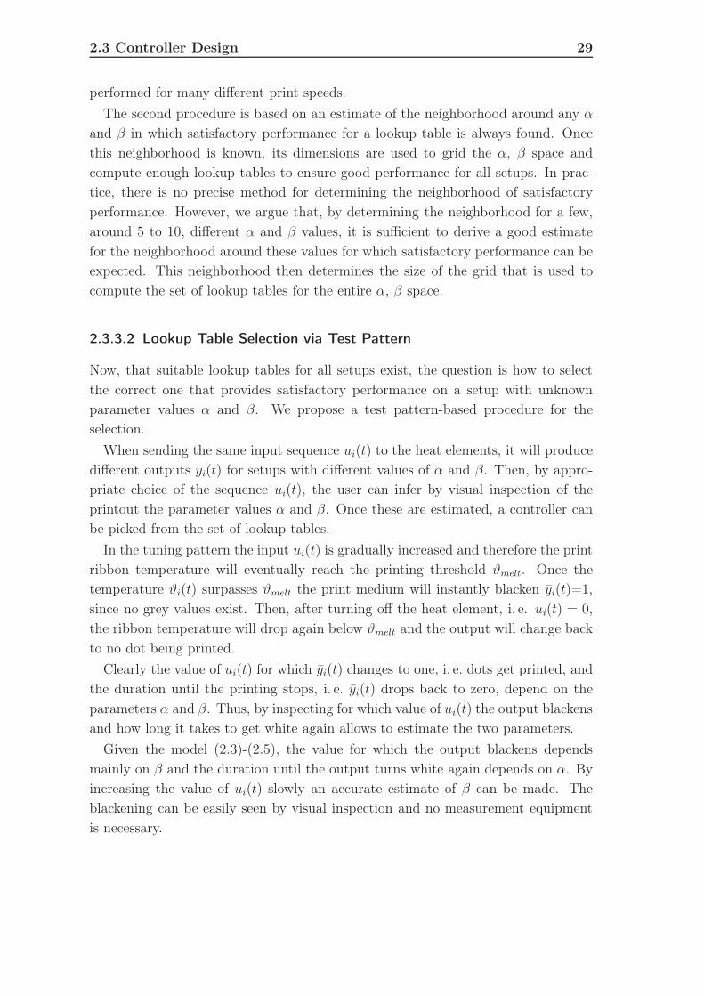
2.3 Controller Design 29
performed for many different print speeds.
The second procedure is based on an estimate of the neighborhood around any α
and β in which satisfactory performance for a lookup table is always found. Oncethis neighborhood is known, its dimensions are used to grid the α, β space andcompute enough lookup tables to ensure good performance for all setups. In prac-tice, there is no precise method for determining the neighborhood of satisfactoryperformance. However, we argue that, by determining the neighborhood for a few,around 5 to 10, different α and β values, it is sufficient to derive a good estimatefor the neighborhood around these values for which satisfactory performance can beexpected. This neighborhood then determines the size of the grid that is used tocompute the set of lookup tables for the entire α, β space.
2.3.3.2 Lookup Table Selection via Test Pattern
Now, that suitable lookup tables for all setups exist, the question is how to selectthe correct one that provides satisfactory performance on a setup with unknownparameter values α and β. We propose a test pattern-based procedure for theselection.
When sending the same input sequence ui(t) to the heat elements, it will producedifferent outputs yi(t) for setups with different values of α and β. Then, by appro-priate choice of the sequence ui(t), the user can infer by visual inspection of theprintout the parameter values α and β. Once these are estimated, a controller canbe picked from the set of lookup tables.
In the tuning pattern the input ui(t) is gradually increased and therefore the printribbon temperature will eventually reach the printing threshold ϑmelt. Once thetemperature ϑi(t) surpasses ϑmelt the print medium will instantly blacken yi(t)=1,since no grey values exist. Then, after turning off the heat element, i. e. ui(t) = 0,the ribbon temperature will drop again below ϑmelt and the output will change backto no dot being printed.
Clearly the value of ui(t) for which yi(t) changes to one, i. e. dots get printed, andthe duration until the printing stops, i. e. yi(t) drops back to zero, depend on theparameters α and β. Thus, by inspecting for which value of ui(t) the output blackensand how long it takes to get white again allows to estimate the two parameters.
Given the model (2.3)-(2.5), the value for which the output blackens dependsmainly on β and the duration until the output turns white again depends on α. Byincreasing the value of ui(t) slowly an accurate estimate of β can be made. Theblackening can be easily seen by visual inspection and no measurement equipmentis necessary.

30 2. Thermal Printhead Control
With parameter estimates, a lookup table that provides satisfactory performancecan be selected from the computed set of tables. Experimental results of this ap-proach are shown in the next section.
2.4 Experimental Results
The proposed control algorithm is tested in simulations and on an experimentalsetup. For the experimental tests, a printer from Avery Dennison is used as areference system. The printer is equipped with a 300 DPI printhead from Rohm.This setup is typical. It is used for ticketing applications or printing of labels forlogistics. Conclusions based on this setup may be extended to cheaper, point ofsales type of applications or to more sophisticated applications for printing highresolution images (e. g. photos or x-ray images).
2.4.1 Identification and Optimal Controller Design
The analysis follows the design steps described in Sections 2.2.2 to 2.3.3 and startswith the identification of the model parameters. For the identification, differentsetups are prepared. Every setup consists of a combination of a ribbon, a printingmedium and a printhead. The influences from the surroundings such as ambienttemperature and humidity are assumed to be relatively small, difficult to reproduceand therefore neglected in the analysis here.
Printing media in the analysis are as follows: label material, cardboard, PVC foil,and type plate material. For printing ribbons a wax-resin (2740) and two differentresin (2560, B110C) coated ribbons are used. Five different printheads of the samemodel are used to test the influence of changing printheads on the results. Thevalues of the parameters ϑmelt and ϑroom are identified and are given in Table 2.1.Next the setups are assembled and the α, β and σn values for the different setups areidentified as described in Section 2.2.2. In the identification experiments the valueof the standard deviation was found to be always close to σn = 9 ◦C, regardless ofthe setup.
To make the parameters invariant under different sampling times TSample in thesystem, all values of α and β are presented for their continuous time counterpartsα and β, with α = eαTSample and β = (eαTSample − 1) β
α.
The results from these identifications for print speed 4 inch per second are shownin Figure 2.5. The printing medium seems to have the main influence on the param-eters, but it is also interesting to note that, for example, for ribbon 2740 all resultslie in a narrow range of β being between 1.1 · 105 ◦C/sec and 1.8 · 105 ◦C/sec.

2.4 Experimental Results 31
50’000 100’000 150’000 200’000 250’000 300’000-700
-650
-600
-550
-500
-450
-400
-350
-300
α[1
/sec
]
β [◦C/sec]
Ribbon: 2560 2740 B110CStickerCardboardPVCType Pl.
Figure 2.5: Identification results for the parameters α, β at print speed 4 inch/secfor medium ribbon combination (indicated by the symbol) and up to five differentprintheads.
Table 2.1: Parameter values.Parameter Value
Surrounding temperature: ϑroom 29◦CRibbon ink melting temperature: ϑmelt 90◦C

32 2. Thermal Printhead Control
100’000 150’000 200’000 250’000 300’000 350’000-450
-400
-350
-300
-250
-200
α[1
/sec
]
β [◦C/sec]
Ribbon: 2560 2740 B110C
Sticker
Cardboard
PVC
Type Pl.
Figure 2.6: Identification results for the parameters α, β at print speed 2 inch/secfor medium ribbon combination (indicated by the symbol) and up to five differentprintheads.

2.4 Experimental Results 33
80’000 100’000 120’000 140’000 160’000 180’000 200’000-900
-850
-800
-750
-700
-650
-600
α[1
/sec
]
β [◦C/sec]
Ribbon: 2560 2740 B110CStickerCardboardPVCType Pl.
Figure 2.7: Identification results for the parameters α, β at print speed 6 inch/secfor medium ribbon combination (indicated by the symbol) and up to five differentprintheads.

34 2. Thermal Printhead Control
Identification results for the print speed of 2 inch per second are shown in Fig-ure 2.6 and identification results for the print speed of 6 inch per second are shownin Figure 2.7. In these plots it can be seen that the β values of the identificationresults do not vary much if the medium ribbon combination is kept and only theprinthead is changed. For example for printing on sticker material using ribbon 2560the β values for the different printheads are within one fifth of the full range of iden-tified β values. To confirm the validity of the approach, the identifications, includingprintout, scanning and identification of α and β values, are repeated for two setups.The results from 14 repeated identifications show that the β value varies only up to10% and the α value varies up to 23%. Within these variations any controller musthave satisfactory performance; otherwise, the printing quality might vary from oneprintout to the next.
In the next step, lookup tables are computed for the identified setups as describedin Section 2.3.1. For the lookup table computations we chose kpast = kfuture = 3.For a print speed of 4 inch/sec more than two third of the influence from the initialtemperature decays over the print duration of 3 dots. Thus every lookup table holds27different dot sequences from which any dot reference pattern can be constructed.
For a frequently used setup, printing on sticker medium using the ribbon 2560, adetailed performance analysis is made. Barcodes are chosen as images since theseare well defined and their printout quality can be validated with appropriate mea-surement equipment, see DIN Norm (3). The results from these tests are shownin Table 2.2. The measurements are made by Avery Dennison. They compare thecurrently implemented controller (Avery) to the proposed controller (ETH). Theresults show that the barcodes printed with an ETH controller are on average oneANSI grade ISO (7) better than those printed with the current printhead controller.
To illustrate this difference, a comparison of the outputs between the currentlyimplemented controller and the proposed controller is shown in Figure 2.8. Thesimulations use the model (2.3)-(2.5) and the input signal ui(t) as they are generatedby the currently implemented controller or the proposed controller, respectively. Itappears that the current controller tends to print the lines of the barcode too wide.
2.4.2 Tuning Rule
To make the controller suitable for use in practice, the tuning rule proposed inSection 2.3.3 is implemented as follows. Based on the identification results shownin Figure 2.5, the space of α and β values at print speed 4 inch/sec is determined torange for α from −650 1/sec to −320 1/sec and for β from 0.6·105 ◦C/sec to 230·105 ◦C/sec.

2.4 Experimental Results 35
Figure 2.8: Comparison of barcodes for current and optimized controller printed at4 inch/sec.
Table 2.2: Comparison of the ANSI ratings for the barcodes printed on stickermedium at different speeds on a 300dpi printhead. Modulewidth determines thenumber of dots of the thinnest line in the barcode. ANSI ratings range from 0 to 4,with 4 being the best.
Print Speed Modulewidth ANSI[inch/sec] [dots] Avery ETH
2 3 2.0 3.02 6 3.3 4.04 3 1.0 2.34 6 2.0 3.76 3 0.0 0.36 6 1.0 3.3

36 2. Thermal Printhead Control
As discussed in Section 2.3.3.1, a set of lookup tables needs to be determinedthat provides satisfactory performance for all α, β combinations within this range.A sensitivity analysis is performed to estimate the shape of the region for which alookup table will always provide satisfactory performance. This region determinesthe size of the slices that are used to partition the α, β-space. One lookup table iscomputed per slice.
First a simulation study of the sensitivity of the controller to parameter variationsis performed. In this study a lookup table for a fixed pair α, β is computed. Theperformance of the lookup table is evaluated in simulations on other α, β pairs. Theresults are plotted in Figure 2.9. The contours show setups for which the lookuptable has equal print quality. The simulation study indicates that the controller isinsensitive to α variations and more sensitive to β variations.
Experiments are conducted to verify the analysis from the simulations. Further-more the results from the experiments will be used to choose for which values ofα and β lookup tables need to be computed in order to have controllers with sat-isfactory performance1 for the entire α, β space. Figure 2.10 shows a result fromexperimental sensitivity analysis. In the experiment, a lookup table is computed forβ = 1.27 · 105 ◦C/sec and α = −526 1/sec. The performance is then tested on all otheridentified setups by printing barcodes. The barcodes are evaluated according to theANSI grade system, see ISO (7). The contours in the figure are generated usinga triangle based linear interpolation that is computed with the Matlab commandgriddata. The contours are used to illustrate where lookup tables with equal printquality are expected. It can be seen in Figure 2.10 that the controller performsvery well for a mismatch in β of ±2 · 104 ◦C/sec and a mismatch in α that covers theentire range of α values. This qualitatively confirms the results from the simulationstudy. The results from the measurements are used to estimate the smallest regionof satisfactory performance.
The findings are supported by further experiments that are carried out for printspeeds of 4 inch per second, see Figures 2.11 and 2.12. In both figures the controllergives satisfactory performance, when printing on setups with α and β values thatare similar to the ones for which the controller is designed. It is also seen from theplots that the sensitivity to variations in α is rather low.
The experiment is repeated for 16 additional setups and more than 300 ANSIgrade measurements are taken in total. These include examples for printing at 2 or6 inch per second, see Figures 2.13, 2.14 and 2.15.
1We define satisfactory performance to be achieved if printed barcodes are rated on average to bebetter than two on the ANSI rating scale, see ISO (7). Note that printer manufacturers mayuse a different definitions of what qualifies as satisfactory performance.
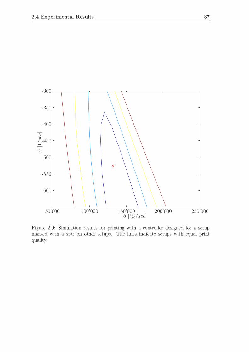
2.4 Experimental Results 37
50’000 100’000 150’000 200’000 250’000
-600
-550
-500
-450
-400
-350
-300
α[1
/sec
]
β [◦C/sec]
Figure 2.9: Simulation results for printing with a controller designed for a setupmarked with a star on other setups. The lines indicate setups with equal printquality.

38 2. Thermal Printhead Control
50’000 100’000 150’000 200’000 250’000
-600
-550
-500
-450
-400
-350
-300
α[1
/sec
]
β [◦C/sec]
Quality: Symbolgood (ANSI ≥ 3)poor (ANSI ≥ 1)insuff. (ANSI = 0)Controller for:
Figure 2.10: Experimental results for printing with 4 inch per second with a con-troller designed for printing on type-plate material using ribbon B110C (markedwith a star) on other setups. Quality is evaluated using ANSI Grades. The lines areused to illustrate where setups with equal print quality might be expected.
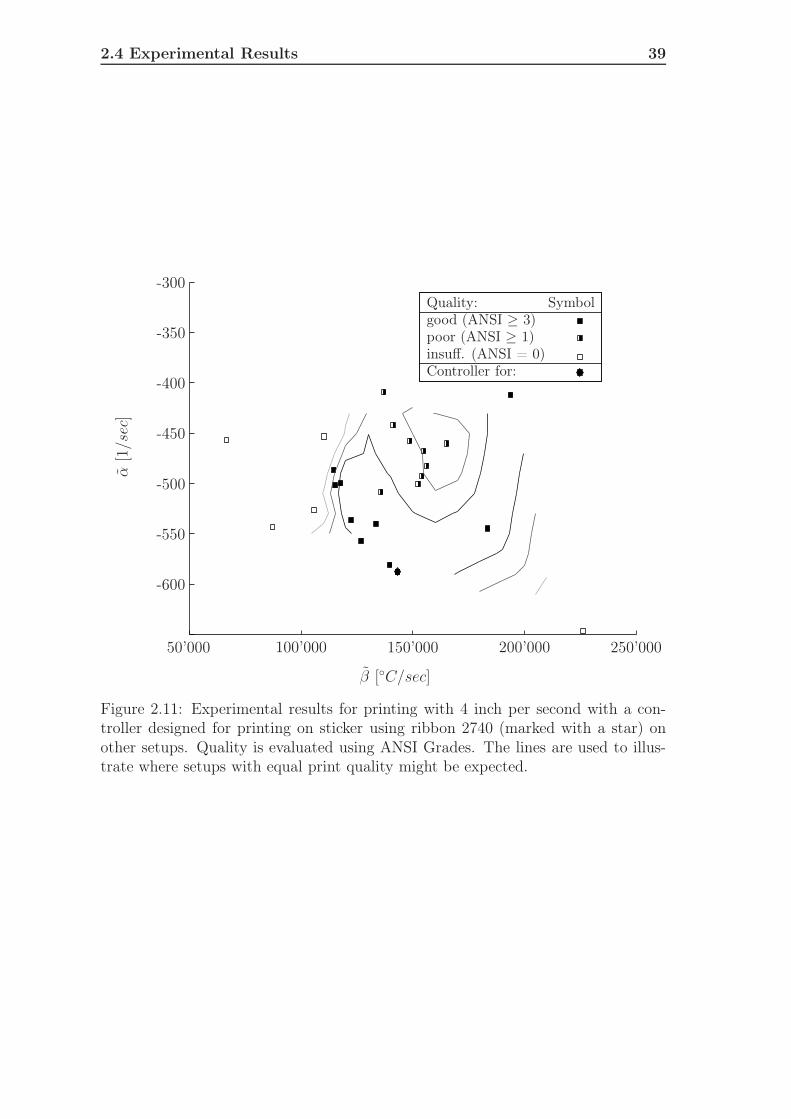
2.4 Experimental Results 39
50’000 100’000 150’000 200’000 250’000
-600
-550
-500
-450
-400
-350
-300
α[1
/sec
]
β [◦C/sec]
Quality: Symbolgood (ANSI ≥ 3)poor (ANSI ≥ 1)insuff. (ANSI = 0)Controller for:
Figure 2.11: Experimental results for printing with 4 inch per second with a con-troller designed for printing on sticker using ribbon 2740 (marked with a star) onother setups. Quality is evaluated using ANSI Grades. The lines are used to illus-trate where setups with equal print quality might be expected.

40 2. Thermal Printhead Control
50’000 100’000 150’000 200’000 250’000
-600
-550
-500
-450
-400
-350
-300
α[1
/sec
]
β [◦C/sec]
Quality: Symbolgood (ANSI ≥ 3)poor (ANSI ≥ 1)insuff. (ANSI = 0)Controller for:
Figure 2.12: Experimental results for printing with 4 inch per second with a con-troller designed for printing on PVC using ribbon 2560 (marked with a star) on othersetups. Quality is evaluated using ANSI Grades. The lines are used to illustratewhere setups with equal print quality might be expected.

2.4 Experimental Results 41
The measurements qualitatively confirm the results from the experiments shownin Figure 2.10, 2.11 and 2.12. However, for some setups a lookup table with sufficientperformance cannot be found. An examples where no sufficient performance is foundis shown in Figure 2.16.
In most cases where, when examples with insufficient print quality are found withα and β values that are close to the values for which the lookup table is designed,these are due to setups that are in general difficult to print on. For example inFigure 2.16 insufficient results are found for a setup with β = 1.15 · 105 ◦C/sec andα = −733 1/sec which is close to the values for which the lookup table is designedfor. However, the setup with the insufficient performance represents printing oncardboard with ribbon 2740. This is a demanding task due to the physical propertiesof the cardboard and the ribbon. In fact, for a difficult media ribbon combinationslike this it might be impossible to get satisfactory performance with any controldesign.
Finally, there are also cases, see for example Figure 2.15, in which the small regionof satisfactory performance is not easily explained. It is only known that for higherprint speeds, starting around 6 inch per second, the printing quality decreases ingeneral and this might also be the case for the example in Figure 2.15.
From this analysis it is determined that eight lookup tables are suitable to coverthe entire α and β range. In fact, for the print speed of 4 inch/second, the partitiononly depends on the β parameter. The strobe input sequences for the eight differentβ values and a fixed α value of −450 1/sec are generated as described in Section 2.3.2.They are stored in a bank of lookup tables. A list of the α and β values is given inTable 2.3.
For a selection of the controllers, a test pattern as shown in Figure 2.17 Is designed.In this test pattern, two lines are printed and the percentage of strobe-on pulsesbetween the lines is increased each time they are printed. At some point the strobe-on percentage will be high enough so that the ribbon ink melts and sticks to themedium. Hence, the area in between the lines will be blackened. In the experimentsit is observed that the percentage highly depends on the value of parameter β. Thus,by printing and visually examining the test pattern, the value of β can be estimated.
Knowing the value of parameter β allows to quickly select a lookup table that islikely to provide satisfactory performance for this setup. Table 2.3 indicates whichlookup table is used when threshold value of x-% strobe on pulses is observed in thetest pattern. With the tuning pattern and the bank of lookup tables, the printercan be used in a stand alone configuration.

42 2. Thermal Printhead Control
100’000 150’000 200’000 250’000 300’000 350’000-450
-400
-350
-300
-250
-200α
[1/s
ec]
β [◦C/sec]
Quality: Symbol
good (ANSI ≥ 3)
poor (ANSI ≥ 1)
insuff. (ANSI = 0)
Controller for:
Figure 2.13: Experimental results for printing with 2 inch per second on with acontroller designed for a setup marked with a star on other setups. Quality isevaluated using ANSI Grades. The lines are used to illustrate where setups withequal print quality might be expected.
Table 2.3: Matching the results from the test pattern evaluation with the computedlookup tables.
Strobe on %: 14% 15% 17% 21% 24% 28% 30% 33%Lookup table: I II III IV V VI VII VIII
Parameters β [105 ◦C/sec] 1.85 1.60 1.35 1.10 1.00 0.90 0.80 0.70α [1/sec] -450 -450 -450 -450 -450 -450 -450 -450

2.4 Experimental Results 43
100’000 150’000 200’000 250’000 300’000 350’000-450
-400
-350
-300
-250
-200
α[1
/sec
]
β [◦C/sec]
Quality: Symbol
good (ANSI ≥ 3)
poor (ANSI ≥ 1)
insuff. (ANSI = 0)
Controller for:
Figure 2.14: Experimental results for printing with 2 inch per second with a con-troller designed for printing on (setup marked with a star) on other setups. Qualityis evaluated using ANSI Grades. The lines are used to illustrate where setups withequal print quality might be expected.

44 2. Thermal Printhead Control
80’000 100’000 120’000 140’000 160’000 180’000 200’000-900
-850
-800
-750
-700
-650
-600
α[1
/sec
]
β [◦C/sec]
Quality: Symbolgood (ANSI ≥ 3)poor (ANSI ≥ 1)insuff. (ANSI = 0)Controller for:
Figure 2.15: Experimental results for printing with 6 inch per second controllerdesigned for a setup marked with a star on other setups. Quality is evaluated usingANSI Grades. The lines are used to illustrate where setups with equal print qualitymight be expected.

2.4 Experimental Results 45
80’000 100’000 120’000 140’000 160’000 180’000 200’000-900
-850
-800
-750
-700
-650
-600α
[1/s
ec]
β [◦C/sec]
Quality: Symbolgood (ANSI ≥ 3)poor (ANSI ≥ 1)insuff. (ANSI = 0)Controller for:
Figure 2.16: Experimental results for printing with 6 inch per second a controllerdesigned for a setup marked with a star on other setups. Quality is evaluated usingANSI Grades. The lines are used to illustrate where setups with equal print qualitymight be expected.
18% 19% 21% 22% 23% 24%strobe on pulses
Threshold reached.
Figure 2.17: Test pattern for tuning. The percentage of strobe-on pulses betweenthe lines is gradually increased, at some point the printing threshold is reached andthe area in-between blackens.
46 2. Thermal Printhead Control
2.4.3 Results
The robust performance of the proposed controller is verified by experiments. Forthe print speed 4 inch/sec, we test 27 combinations of ribbons, print mediums anddifferent printheads. The experiments are conducted with three different printheads.Table 2.4 summarizes results for a new printhead (#1), that has been used duringprevious identification experiments. For the measurements in Table 2.5, we usea printhead (#6) that has undergone a stress test previously, i. e., represents aprinthead after heavy use. Table 2.6 shows results with a printhead (#5) that hasnot been used for experiments previously.
In the first two columns of Table 2.4, 2.5, and 2.6, the ribbon code and the printingmedium are specified. For each setup the current implementation (Avery) and theproposed controller (ETH) are tested. For the current controller, the parametersare tuned by repetitive adjustments and measurements until the optimal tuning ofthe implemented controller is found. For the proposed controller, the test pattern isprinted and the appropriate controller is selected through the mapping in Table 2.3.It has to be noted that the proposed scheme is simpler and faster than the currentscheme, which requires much printing and scanning of printouts for tuning. Theevaluation of the printouts is made according to the ISO norm, see DIN Norm(3). Three measurements of each printout are taken. The average of the threemeasurements is given in the last two columns of the tables.
Clearly, both controllers perform well. At least for the common modulewidth of5 dots, no barcode is classified as non-readable. In addition, the ETH controllerperforms slightly better on average. For a more extreme case of printing barcodeswith modulewidth 2 dots, the difference becomes more obvious. For some setups, itis not possible to tune the current controller to produce readable outputs. Never-theless, on these setups the ETH controller produces acceptable results. Note thatthe modulewidth 2 analysis is performed with a printhead that has not been usedfor any tests or during the algorithm design before.
2.5 Conclusions
In this part we present a model based approach for the development of a controllerfor a thermal printhead. The printhead input-output behavior is modeled by a firstorder linear system and a nonlinear output mapping, including a stochastic variableto account for the uncertainty in the system. The model is used in a mathematicalprogram to compute the optimal input signals for the printhead.
A tuning concept is introduced to achieve good performance on a variety of print-

2.5 Conclusions 47
Table 2.4: Performance evaluation for: Speed 4 inch/sec · Modulewidth 5 · Print-head# 1(new)
Setup ANSIRibbon Medium Avery ETH2560 Cardboard 0.33 2.662560 Sticker 1.33 1.002560 Type Pl. 2.66 3.002560 PVC 4.00 0.662740 Cardboard 4.00 4.002740 Sticker 2.00 3.002740 Type Pl. 1.66 3.332740 PVC 4.00 3.00
B110C Type Pl. 3.00 3.33
Table 2.5: Performance evaluation for: Speed 4 inch/sec · Modulewidth 5 · Print-head# 6 (stress tested)
Setup ANSIRibbon Medium Avery ETH2560 Cardboard 3.00 4.002560 Sticker 1.00 2.662560 Type Pl. 2.33 3.002560 PVC 3.66 3.002740 Cardboard 3.00 4.002740 Sticker 2.00 2.662740 Type Pl. 3.00 2.662740 PVC 4.00 4.00
B110C Type Pl. 2.33 3.00

48 2. Thermal Printhead Control
Table 2.6: Performance evaluation for: Speed 4 inch/sec · Modulewidth 2 · Print-head# 5 (new, not used during identification experiments)
Setup ANSIRibbon Medium Avery ETH2560 Cardboard fail 1.002560 Sticker 0.00 1.332560 Type Pl. fail 2.002560 PVC 2.00 1.332740 Cardboard 0.33 1.662740 Sticker 1.00 0.662740 Type Pl. 0.66 1.332740 PVC 0.33 1.33
B110C Type Pl. 0.33 2.66
ing setups including: different print media, ribbons or printheads. In experiments,robustness and performance of the tuning concept is demonstrated. In general,the newly proposed controller outperforms the current implementation in a ther-mal printer. Furthermore, the new controller can be tuned by printing a simpletest pattern and reading off the result. This tuning concept is simpler and fasterthan current trial and error methods. The evaluation demonstrates suitability ofthe proposed controller for use in practice.
Acknowledgments
The work is supported by Avery Dennison Deutschland GmbH and Rohm Ltd. Theauthors thank Raphael Cagienard for his support.

Bibliography 49
Bibliography
[1] Cplex (2006). ILOG CPLEX 10.0 User’s Maual. ILOG, France.
[2] DIN Norm (1995). Einflussgroessen auf die Lesung von Strichcodes, DIN ENV
1649. Normenausschuss Daten- und Warenverkehr in der Konsumgueterwirtschaftim DIN Deutsches Institut fuer Normung e.V.
[3] DIN Norm (1998). Strichcodierung, Pruefungsanforderungen fuer Strichcode-
Pruefgeraete, DIN ENV 12647. Normenausschuss Daten- und Warenverkehrin der Konsumgueterwirtschaft im DIN Deutsches Institut fuer Normung e.V.,12.1998 edition.
[4] Drees, F., Grethen, H., Nisius, R., & Pekruhn, W. (1989). Performances of ther-mal transfer printing and their improvement by model calculations. In CompEuro
’89., ’VLSI and Computer Peripherals. VLSI and Microelectronic Applications
in Intelligent Peripherals and their Interconnection Networks’, Proceedings. (pp.2/40–2/42).
[5] Fukushima, I. (2006). New intelligent thermal printing technology. In IS&T’s
NIP22: International Conference on Digital Printing Technologies (pp. 268–271).
[6] Günther, S. & Wölm, D. (1996). Patent 96101152.5, Druckkopfthermosteuerung
(in German). European Patent Office.
[7] ISO (2000). ISO/IEC 15416, Information technology - Automatic identification
and data capture techniques - Bar code print quality test specification - Linear
symbols.
[8] Kyocera (2001). Thermal printhead products - application notes,http://global.kyocera.com/prdct/ios/tph/index_tech.html. Manual and Techni-cal Specifications.
[9] Lide, D. (2005). CRC handbook of chemistry and physics. Boca Raton.
[10] Rohm, Printhead Division (2003). Thermal printhead application manual - ba-sic edition ver1.00, http://www.rohm.com/products/module/printhead. Manual.
[11] Ruszczynski, A. & Shapiro, A. (2003). Stochastic Programming (Handbooks in
Operations Research and Management Series). Elsevier Publishing Company.
[12] Shibata, S. (1995). Thin-film thermal head with heating resistors having self-controlled temperature. In Industry Applications Conference, 1995. Thirtieth IAS

50 Bibliography
Annual Meeting, IAS ’95., Conference Record of the 1995 IEEE, volume 3 (pp.1976–1981 vol.3).
[13] Shigeru, A. & Masanori, S. (1987). Patent, 62227664 A, Thermal Printer Print
Control System (in Japanese). Alps Electric Co Ltd, Japanese Patent Office.
[14] Tsubone, K., Osumi, T., Ishizaki, T., Shinohara, M., Suzuki, M., Matsumi, K.,& Akahane, K. (1988). A smart bicmos driver for 400 dpi thermal printing heads.In Custom Integrated Circuits Conference, 1988., Proceedings of the IEEE 1988
(pp. 5.2/1–5.2/4).

Bibliography 51


Part II
Load Tracking Scheduling
53


3 Comparison of Continuous and
Discrete Time Formulations for
Load Tracking Scheduling
Problems
3.1 Introduction
Scheduling deals with the allocation of resources and tasks in order to accomplishprocesses. Examples of processes include manufacturing of goods or the provisionof services. The tasks are the steps needed to accomplish the processes and theresources specify objects that are needed to perform the tasks. Finding a “good”allocation of the resources and tasks can have significant impact on the cost andperformance of a process.
Scheduling is an active field of research. The publications Mendez et al. (46),Floudas & Lin (35), Floudas & Li (34) and Pinto & Grossmann (55) present a goodoverview on current methods and trends. Despite the advances in the research nosingle mathematical method is in general proven to be superior when applied tocommon scheduling problems. Not all methods exhibit the same modeling capa-bilities and thus the used method to solve a particular scheduling problem alwaysdepends on the structure of the problem.
Some guidance on choosing the right modeling method can be found in the litera-ture; see for example Möhring (50), Mendez et al. (46), Maravelias & Grossmann (45)and Castro & Grossmann (20). However, these publications only provide guidelinesfor classical scheduling problems such as makespan or production cost minimizationand revenue maximization.
This paper extends the comparison of scheduling models by focusing on the prob-lem of load tracking scheduling, a non-traditional scheduling problem. In load track-ing scheduling, tasks have to be performed so that a pre-specified production orconsumption is fulfilled in a best possible manner at each time. Load tracking prob-lems occur during shift planning for workers in call centers, hospitals, retail stores
55

56 3. Load Tracking Scheduling
or airports, where the load is derived from the expected customer frequency, seeDi Gaspero et al. (27), Al-Yakoob & Sherali (3), Bard et al. (5), Bard & Purnomo(6), Buffa et al. (17), Ernst et al. (31) and Eveborn & Ronnqvist (32) for examples.
A specific variation of load tracking scheduling is level scheduling. In level schedul-ing tasks are allocated such that the production or consumption is the same at alltimes. Level scheduling is used in Just-In-Time production, where the output ofparts must be kept constant to fulfill a constant demand. For introductory refer-ences to Just-In-Time production see Miltenburg (48), Sugimori et al. (59), and forlevel scheduling for Just-In-Time production see also Kubiak et al. (42), Steiner &Yeomans (58) and Drexl et al. (28).
The difference between load tracking and classical scheduling problems is thatthe objective of load tracking scheduling is to assign tasks so that the sum of con-sumption or production at each time point matches the pre-specified (load tracking)or constant (level scheduling) load. Classical scheduling objectives differ to loadtracking scheduling. Classical objectives are to minimize makespan, earliness orproduction cost. In contrast to load tracking scheduling they do not penalize pro-duction or consumption at every time point, but minimize production duration orconsumption over the entire scheduling horizon.
For classical scheduling problems comparisons between different model formula-tions exist, see Castro & Grossmann (20) and Mendez et al. (46). For examplein Castro & Grossmann (20) it is shown that for scheduling problems minimizingtotal earliness using a scheduling formulation that discretized time performed best.However, the paper also shows counterexamples, where for specific instances a for-mulation modeling time as a continuous variable leads to better results.
The special structure of load tracking scheduling problems makes it difficult toinfer from the results for classical scheduling problems which modeling method wouldbe more beneficial. Therefore, we compare two modeling methods that have beensuccessfully applied in classical scheduling for load tracking scheduling. The methodsdiffer in their representation of time. One treats time as a continuous variablewhereas the other uses a time discretization. Both methods result in a mathematicalprogramming problem with continuous and discrete decision variables that havelinear constraints and objectives. Thus, these problems can be solved using mixed-integer linear programming solvers.
The structure of the two different models considered will be explained in Sec-tion 3.2. In Section 3.3 two test cases, the demand driven scheduling of employeeshifts and the energy cost optimal scheduling of a steel plant, will be presented.Formulation of each of the two test cases using the different methods are given inSection 3.3.1 and 3.3.2. The formulations are implemented and their performance

3.2 Models for scheduling problems 57
is compared in Section 3.3.1.4 and 3.3.2.4. Conclusions are given in Section 3.4.
3.2 Models for scheduling problems
A rich literature on scheduling exists, including books (see Brucker & Knust (15),Brucker (14), or Pinedo (54)) and journals (e. g. Journal of Scheduling) devotedto the topic. This has created a diverse collection of scheduling models. In thispaper we limit ourselves to models that fall into the class of mixed-integer linearprograms (MILPs). These models offer an advantage in that they can be used todescribe a rich class of scheduling applications, see Grossmann et al. (37). For thecomputation of the scheduling solution, standard MILP solver software can be usedwhich is commercially available such as Xpress-MP from Dash Optimization (Xpress(71)) and Cplex from Ilog (Cplex (25)). Using MILP solver software for schedulingproblems is well established, see Bixby & Rothberg (11) and Ashford (4).
MILP models allow the formulation of scheduling problems that involve discreteand continuous variables and linear equality and inequality constraints. The papersof Pinto & Grossmann (55), Castro & Grossmann (20), Floudas & Li (34), Floudas& Lin (35) and Mendez et al. (46) provide an overview on different schedulingmodels that lead to MILP formulations. A primary difference among the modelsis the representation of time. Older MILP scheduling models use a discrete timerepresentation, e. g. see Bowman (13). This means that the scheduling horizon isdivided into fixed intervals, where events may only happen at these discrete timepoints. Often this leads to problems involving several thousands of binary variablesto attain the desired degree of accuracy in the time representation, see Castro &Grossmann (20). Despite their size, discrete time models are known to work well formany classical scheduling objectives such as makespan minimization (Maravelias &Grossmann (45)).
During the last decade, models representing time as a continuous variable havereceived much attention (Castro & Grossmann (20)). In the continuous time caseevents can happen at arbitrary time points. A recent example considering con-tinuous time scheduling for classical objectives of makespan minimization or profitmaximization is given in Janak & Floudas (40).
For classical scheduling objectives it is well known that selecting between a discreteor a continuous time representation has an important impact on the size, complexityand solvability of the model, see Castro & Grossmann (20) and Mendez et al. (46)for a discussion. However, it is not clear how this transfers to the case of loadtracking scheduling that this paper is concerned with. The paper therefore presents

58 3. Load Tracking Scheduling
discrete and continuous time formulations for load tracking scheduling problems,implements them and compares their performance.
In both discrete and continuous time formulations tasks l ∈ L are assigned toresources i ∈ I that are needed to accomplish the tasks. The discrete time and con-tinuous time formulations for the load tracking scheduling problem are introducedin Subsections 3.2.1 and 3.2.2.
3.2.1 Discrete Time Models
In the discrete time models considered in the paper the time variable is discretizedat a uniform rate, TSample. All events, changes from one machine to another, etc.can only take place at multiples of this sampling rate. Therefore, all events affectingthe schedule, such as start or end of a task, can only take place at specific instances.Essentially, this leads to an approximation of the solution that would allow for eventsat arbitrary time points.
Depending on the tasks included in the system, the discretization rate Tsample
needs to be chosen. For the special case of tasks with fixed time durations thegreatest common factor can be used as a sampling time to obtain an exact solution.However, in practical situations this factor can be very small leading to a very finetime discretization which makes the problem computationally too expensive. Anexact discretization stops existing as soon as tasks are allowed to start at arbitrarytime points and their duration is given by a time range.
The advantage of discrete time scheduling models is that time discretization pro-vides a common reference grid and restrictions on equipment use, etc. can be formu-lated relatively easily. Also estimating and tuning the problem size by changing thediscretization rate TSample is simple since the number of variables changes linearly.
To illustrate discrete time modeling, typical constraints are presented for twoformulations with different consideration of events. In the first formulation, theconstraints are given as linear inequalities. This type of formulation represents astandard technique that is usually found in the literature, see Floudas & Lin (35).The formulation assumes no special structure on the events. It is presented inSection 3.2.1.1.
The second discrete time formulation is presented in Section 3.2.1.2. It is derivedby examining the scheduling problem from a control engineering point of view. Inthis formulation events are triggered by input signals. and the scheduling problemis models as a hybrid system, which is a system involving continuous and discretedynamics. It is successfully applied by Gallestey et al. (36).

3.2 Models for scheduling problems 59
3.2.1.1 General Discrete Time Scheduling Models
In the general case consider a task l at time t ∈ T , with T = {0, . . . , Tmax} andTmax being the planning horizon length. Then the state, indicating whether thetask l is being performed at time t, can be represented as a binary variable δl,t. Thevariable takes value 1 if the assignment is true and 0 if the assignment is false. Thisrepresentation easily allows to impose constraints. If all tasks using resource i areincluded in the set Li then we can constrain that at each time t only one task canrun on machine i by requiring:
∑
l∈Li
δl,t ≤ 1 ∀t ∈ T . (3.1)
Also it is simple to compute the total usage ui of resource i by all tasks, since itcan be rewritten as a sum:
ui =∑
t∈T
∑
l∈Li
δl,t (3.2)
and thus limits umini or umax
i on the total work done using resource i can beimposed by:
umini ≤ ui ≤ umax
i .
Objectives such as usage minimization of resource j are simple to model asmin
∑i ui. In discrete time modeling many requirements can be easily formulated
by linear constraints since the variables δl,t contain explicit information about thesystem state at each time t.
3.2.1.2 Mixed Logic Dynamical Models
Examining the scheduling problem from a control engineering point of view raisesthe idea of using one of the available frameworks for systems with coupled discreteand continuous variables. Such systems are also known as hybrid systems andare described by Heemels et al. (39), Davoren & Nerode (26). In hybrid systemsthe state of the systems is stored in a vector of continuous and discrete variables.Evolution of the state is described by the system inputs and the system equations.The idea is to use a hybrid system description to store the system state and restrictpossible transitions and inputs to those that do not violate any scheduling rules. Aschedule is obtained by optimization of a cost function with the system equations asconstraints and the inputs being the decision variables in the optimization problem..
One framework that can be used in this respect is the Mixed Logical Dynamical

60 3. Load Tracking Scheduling
(MLD) Systems framework (Bemporad & Morari (9)). It is based on the conceptthat logical relations can be reformulated into mixed-integer inequalities automati-cally, see Morari et al. (51), Raman & Grossmann (56), Raman & Grossmann (57),Tyler & Morari (66) and Williams (70). The modeling language HYSDEL supportsmodel constraints using propositional logic and has a compiler that translates thelogic formulation into mixed-integer inequalities (Torrisi & Bemporad (63)).
Some examples for automatic reformulation of propositional logic into mixed-integer linear constraints are given in Table 3.1. Using common notation Xn rep-resents a literal that has a truth value, either false or true. Different literals areconnected by operators not (¬), and (∧), or (∨), xor (⊕), implies (⇒) and if andonly if (⇔) to map to a resulting truth value. In the reformulation, literals are writ-ten as binary variables δn ∈ {0, 1} with value 1 being associated with Xn being trueand 0 meaning that Xn is false. By constraining the δn variables, one can formu-late statements that are equivalent to those formulated using the literals and logicoperators. The statements using the δn variables can be evaluated using constraintprogramming or mixed-integer programming techniques.
Table 3.1 also provides two examples on how to link continuous variables withlogic. These are the Analog-Digital and the Digital-Analog relation. They leadto mixed-integer linear inequalities as constraints. The generation of this type ofconstraints is based on the big M technique. The variables Mn and mn are upperand lower bounds on the values that fn(x) can take. An overview of how to usethe big M technique to reformulate a variety of mixed logic propositions, involvingcontinuous variables and literals, is given by Mignone (47).
Using the relations from Table 3.1 any combinatorial relation of logic variablescan be described. With the inclusion of the Digital-Analog and Analog-Digitalrelations and linear dynamic difference equations, hybrid systems can be modeledusing propositional logic and then transformed into the form of an MLD system.MLD systems are given by:
x(k + 1) = A0 x(k) + B1 u(k) + B2 δ(k) + B3 z(k) + B5 (3.3)
y(k) = C0 x(k) + D1 u(k) + D2 δ(k) + D3 z(k) + D5 (3.4)
E2 δ(k) + E3 z(k) ≤ E1 u(k) + E4 x(k) + E5 (3.5)
E2 δ(k) + E3 z(k) = E1 u(k) + E4 x(k) + E5 (3.6)
with x ∈ Rnr×{0, 1}nb as a vector of continuous and binary states, u ∈ R
mr×{0, 1}mb
as inputs, y ∈ Rpr × {0, 1}pb as outputs, z ∈ R
rr as continuous and δ ∈ {0, 1}rb asdiscrete auxiliary variables, and A0, B1, B2, B3, B5, C0, D1, D2, D3, D5, E1, E2,

3.2 Models for scheduling problems 61
Table 3.1: Logic relations and their conversions into mixed-integer relations.Relation Logic Proposition Constraint
NOT ¬X1 δ1 = 0AND X1 ∧X2 δ1 = 1; δ2 = 1OR X1 ∨X2 δ1 + δ2 ≥ 1
XOR X1 ⊕X2 δ1 + δ2 = 1IMPLICATION X1 → X2 δ1 − δ2 ≤ 0
IFF X1 ↔ X2 δ1 − δ2 = 0
Analog-Digital [f(x) ≤ 0]↔ [δ = 1]f(x) ≤M(1− δ)
f(x) ≥ ǫ + (m− ǫ)δ
Digital-Analog X→[f(x)=0]m(1− δ) ≤ f(x)M(1− δ) ≥ f(x)
E3, E4, E5, E1, E2, E3, E4, E5 being system matrices of suitable dimension. Itis shown that this type of system is equivalent to many other well known modelsof hybrid systems such as linear complementarity (LC) systems, extended linearcomplementarity (ELC) systems, piecewise affine (PWA) systems, and max-min-plusscaling (MMPS) systems. Some of the equivalences are established under (rathermild) additional assumptions, see Heemels et al. (39).
There is no established way in how to use the MLD system and the propositionallogic for the formulation of a scheduling problem. However, in Gallestey et al. (36)and Ferrari-Trecate et al. (33) the authors choose to formulate timers as conditionedstate update equations. For example, δl(t) can indicate whether task l is active attime t. Then xl(t) is a timer counting the duration of task l:
δl(t) = 1⇔ xl(t + 1) = x(t) + 1 . (3.7)
Requirements arising from the physical plant are modeled as constraints on the inputvariables ul. For example, an input signal of ul that changes the activity of xl mightbe restricted to zero, unless a minimum processing time Tmin
l has passed:
xl(t) < Tminl ⇒ ul(t) = 0 . (3.8)
A compiler, for example HYSDEL (Torrisi et al. (65)) can convert the logic for-mulations in (3.7) and (3.8) into mixed-integer linear constraints (3.3)-(3.6). Themixed-integer inequalities from equations (3.3)-(3.6) ensure that a feasible solutionis found. Thus they are used as constraints in an optimization problem that com-putes a schedule. However, the advantage of using logic formulations comes at thecost of having a compiler-generated formulation that is in general not as compact in

62 3. Load Tracking Scheduling
terms of the number of variables and constraints as a formulation that is generatedby direct translation of the process requirement into inequality constraints. Espe-cially, for constraints involving big M formulations a compiler usually chooses tooconservative values for Mn and mn.
3.2.2 Continuous Time Models
In continuous time models no sampling time is needed. The occurrence of eventscan happen at any time. The timing of the events is stored in continuous variables,with starting time of the task l denoted tsl and the ending time tel . Using thisrepresentation, a constraint such as requiring the minimum processing durationTmin
l can be modeled astel − tsl ≥ Tmin
l . (3.9)
Note that this constraint includes the obvious requirement that the starting timeof a task is before its ending time. A constraint on the maximum task durationTmax
l can be modeled in analogous way:
tel − tsl ≤ Tmaxl . (3.10)
However, modeling constraints that require the state of a task at certain timesis more complex. An example of such a constraint would be two tasks l′ and l′′
sharing a resource i. If only one of the tasks can be processed at a time a constraintthat prevents collisions must be included. This is done by requiring either task l′ tohappen before l′′ :
tel′ − tsl′′ ≤ 0 (3.11)
or vice versa:tel′′ − tsl′ ≤ 0. (3.12)
To model this or-type of constraint a big M technique is used. In the big Mformulation, a binary variable δl′,l′′ is introduced that ensures that exactly one ofthe two constraints is active. The parameter big M is chosen as an upper boundon the time separating the ending of one and the starting of the other task. Themutual exclusion of the constraints using resource i is modeled by:
tel′ − tsl′′ ≤ M(1− δl′,l′′) (3.13)
tel′′ − tsl′ ≤M δl′,l′′ . (3.14)

3.3 Examples of Load Tracking Scheduling Problems 63
Note that in a discrete formulation the exclusion could be modeled by simplyrequiring that at each time k the sum of the δl,k is less than one, see equation (3.1).In the continuous time, the state at time t is not explicitly available and has tobe recovered from the relation of starting and ending times of the tasks. This maysignificantly complicate the modeling.
3.3 Examples of Load Tracking Scheduling
Problems
To test the performance of the discrete time and continuous time models for loadtracking problems we introduce two examples. The first problem, dealing withthe assignment of employees to shifts so that a given employee demand is satisfiedat all times, is presented in Section 3.3.1. The second problem describes a steelmanufacturing problem where the electrical load of the plant is supposed to track apre-specified load curve, Section 3.3.2.
3.3.1 Employee Scheduling
In employee scheduling, timetables for staff are created so that an organizationcan optimally satisfy the requirements for its production or services. This involvesdetermining the number of staff members with particular skills needed to meet thedemand. The staff members are then allocated to shifts so as to meet the requiredstaffing levels at different times. Furthermore, duties are assigned to individualsfor each shift. All industrial regulations associated with the relevant workplaceagreements must be observed during the process.
The problem is to find an optimal or at least a good feasible solution that mini-mizes costs, meets employee preferences, distributes shifts equitably among employ-ees and satisfies all the workplace constraints. A number of survey papers have beendevoted to the general area of personnel scheduling, see Caprara et al. (19), Ernstet al. (31), Ernst et al. (30), Tien & Kamiyama (62).
In Caprara et al. (19) different mathematical models for staff scheduling that usea two stage decomposition are presented. In the first stage of the problem, the shiftsare computed that need to be scheduled and in a second stage an assignment of theemployees to the shifts is made. The paper of Tien & Kamiyama (62) decomposes thescheduling problem even further, for example they formulate break shift schedulingas a separate component. In their paper, Tien & Kamiyama (62) review differentmodels to solve these sub-problems. The papers of Ernst et al. (31) and Ernst et al.

64 3. Load Tracking Scheduling
(30) provide a general overview by briefly reviewing a wide range of papers writtenon scheduling.
Also, the problem of demand driven personnel scheduling has received attentionin the survey papers. In the papers of Burke et al. (18) and Cheang et al. (21) theauthors examine the problems of nurse scheduling and call center operator schedul-ing. In those problems the shifts must be scheduled such that a pre-specified loadis tracked and working regulations are fulfilled.
Models of personnel scheduling problem can be subdivided into those using formu-lations leading to MILPs or ILPs that are either solved directly using MILP solversoftware (see Al-Yakoob & Sherali (3), Kwan & Kwan (44), Bard & Purnomo (6),Belien & Demeulemeester (8), Belien & Demeulemeester (7), Eveborn & Ronnqvist(32), Jaumard et al. (41), Wan & Bard (68), Berrada et al. (10), Valouxis & Housos(67), Addou & Soumis (1), Bard et al. (5) and Corominas et al. (24)) and those us-ing more general formulations leading to non-linear problems that are not solvableusing MILP solvers and rely on heuristics and stochastic search methods (see Buffaet al. (17), Aickelin & Li (2), Brusco & Jacobs (16), Chuin Lau (22), Watson et al.(69) and Mirrazavi & Beringer (49)).
3.3.1.1 Requirements and Objective
The problem under consideration is motivated by scheduling problems in serviceindustry. The goal is to allocate employee shifts such that the employee presencematches the demand, while fulfilling all regulatory constraints.
The objective is to minimize the difference between allocated employees i ∈ I,where I is the set of all employees, and employee demand at a given time. Thedemand is given by demand intervals indexed by n ∈ N . Each interval is a 2-tuplegiven by (tdn, qn) ∈ E , with tdn being the starting time of the demand interval andqn being the demand of interval n. The demand requirement has to be trackedcontinuously during the interval. The intervals are ordered and cover the entiretime horizon, thus tdn+1,the starting time of interval n+1, is the end time of intervaln. To simplify formulation of the constraints, the end of the last interval is definedas tn|N |+1 . In the objective, both overstaffing, i. e. allocation of more employees thandemanded by qn, or understaffing, i. e. allocation of fewer employees than demandedby qn, is to be penalized.
In addition to the objective, we pose requirements that have to be fulfilled. Fromthe service providers’ point of view, it is necessary to constrain shift start andend times to be within the opening or service hours ranging from Topento Tclose.Secondly, the service provider requires a minimum level of presence during the service

3.3 Examples of Load Tracking Scheduling Problems 65
hours regardless of the specified demand. The minimum service level is specified byrequiring a presence of Pmin employees at all time.
From the employees point of view, we constrain the number of shifts to be amaximum of one per day. In addition the shift length is constrained to be withinT SL
min and T SLmax. In summary the requirements are:
1. time horizon is one working day;
2. each employee works one shift per day;
3. the shift length is subject to a lower and an upper bound;
4. a minimal number of employees is required to be present at all times;
5. the objective is to minimize the deviation between the actual number of em-ployees and the required presence.
Next, these requirements are modeled using a discrete time model, see Section 3.3.1.2,and with a continuous time model, see Section 3.3.1.3.
3.3.1.2 Discrete Time Model
For the employee scheduling problem, we apply discrete time modeling techniquesintroduced in Section 3.2.1.1. Time is discretized at a uniform rate TSample into in-tervals. All events such as employees coming or leaving and changes in the personneldemand can only happen at these time points. The presence or absence of employeei at time t is represented by the binary variable δi,t ∈ {0, 1}, where δi,t = 1 indicatesthat employee i is present from time t until t + 1.
By fulfilling the requirements posed in Section 3.3.1.1 one by one, we constructthe discrete time model:
• Requirement 1: To remain within the opening and closing time, the time indext ∈ T is defined for the set T = {1, . . . , T}, with T = (Tclose − Topen)/TSample.Then the discrete time maps to the continuous time by t TSample + Topen.
• Requirement 2: The requirement that each employee must work one shift perday is equivalent to requiring the employee to be present at at least one timepoint, ∑
t∈T
δi,t ≥ 1, (3.15)

66 3. Load Tracking Scheduling
and to limit the number of times that he starts a shift also to be one. Startingtimes of shifts are modeled by δon
i,t ∈ {0, 1}. They are given by the change inemployee presence from one time index to the next, thus:
δoni,t ≥
T∑
t=2
(δi,t − δi,t−1) ∀i ∈ I, (3.16)
δoni,1 ≥ δi,1 ∀i ∈ I. (3.17)
The shift starts are limited to be one per day,
∑
t∈T
δoni,t ≤ 1 ∀i ∈ I. (3.18)
• Requirement 3: The shift length of each employee has upper and lower boundsT SL
min and T SLmax respectively. Thus the number of presence times δi,t multiplied
by the sampling time Tsample must be bounded as follows:
T SLmin ≤ Tsample
∑
t∈T
δi,t ≤ T SLmax ∀i ∈ I. (3.19)
• Requirement 4: At any time at least the minimum number of employees Pmin
has to be present. This is modeled by requiring for all times t:
∑
i∈I
δi,t ≥ Pmin ∀t ∈ T . (3.20)
• Requirement 5 (Objective): The tracking error et at time t is given by thedifference between
∑i∈I δi,t, the number of employees present at time t, and
the demand requirement qn valid for time t:
et ≥ qn −∑
i∈I
δi,t ∀t ∈ {tdn, . . . , t
dn+1}, n ∈ N , (3.21)
et ≥ −qn +∑
i∈I
δi,t ∀t ∈ {tdn, . . . , t
dn+1}, n ∈ N . (3.22)
The objective is then to minimize the sum over all times t of all the trackingerrors
min∑
t∈T
et. (3.23)

3.3 Examples of Load Tracking Scheduling Problems 67
3.3.1.3 Continuous Time Model
The continuous time formulation presented here is taken from the thesis Conte (23)with minimal changes concerning the generation of event points. For the continuoustime model, events m ∈ M and corresponding event times tm ∈ T are introduced.There are event times for the starting time of an employee i and the finishing time.Also the starting times of each requirement interval n are linked to event times.Thus, the index set of all events isM = {1, . . . , 2 ∗ |I|+ |N |}. The event times areordered:
tm ≥ tm−1 ∀m ∈ {2, . . . , |M|}, (3.24)
and the interval length between two points is given by ∆tm, with
∆tm = tm+1 − tm ∀m ∈ {1, . . . , |M| − 1}. (3.25)
Discrete variables δsi,m, δe
i,m, δnn,m ∈ {0, 1} are introduced to link the event times
tm with the events shift starts, shift ends and requirement interval starts. Thesevariables, i. e. δs
i,m for shift start of employee i, take value 1 if the event happensat tm and 0 otherwise. The continuous time model is constructed by modeling allrequirements posed in Section 3.3.1.1.
• Requirement 1: The store open and closing time requirement is imposed bydefining t ∈ T and
T = {t : t ∈ R, Topen ≤ t ≤ Tclose}. (3.26)
• Requirement 2: By adding the constraints
∑
m∈M
δsi,m = 1 ∀i ∈ I, (3.27)
∑
m∈M
δei,m = 1 ∀i ∈ I, (3.28)
∑
m∈M
δnn,m = 1 ∀n ∈ N , (3.29)
all employee shifts start, end and all sales interval start points belong exactlyto one event point m. By setting
∑
i∈I
δsi,m +
∑
i∈I
δei,m +
∑
n∈N
δnn,m = 1 ∀m ∈M (3.30)
each event time tm is associated with exactly one event. Therefore, each

68 3. Load Tracking Scheduling
employee i has exactly one shift during the day.
• Requirement 3: To constrain the shift length, we first model the presence du-ration pi,m of employee i in the interval between event m and m+1. Therefore,each pi,m is constrained to be equal to the value of ∆tm if the employee startedworking before tm and finishes working after tm. Otherwise pi,m is zero:
pi,m ≤ ∆tm + M(1−m∑
m′=1
(δsi,m′ − δe
i,m′)) (3.31)
∀i ∈ I, m ∈ {1, . . . , |M| − 1},
pi,m ≥ ∆tm −M(1−m∑
m′=1
(δsi,m′ − δe
i,m′)) (3.32)
∀i ∈ I, m ∈ {1, . . . , |M| − 1},
pi,m ≤ M(m∑
m′=1
(δsi,m′ − δe
i,m′)) ∀i ∈ I, m ∈ {1, . . . , |M|}. (3.33)
Big M constraints are used to enforce a time slice pi,m for employee i to takethe value ∆tm or zero.The sum of all time slices for each employee must be within the minimum T SL
min
and maximum T SLmax allowed shift time:
T SLmin ≤
∑
m∈M
pi,m ≤ T SLmax ∀i ∈ I. (3.34)
• Requirement 4: To guarantee Pmin employees from the opening in the morning,we require that the first Pmin event times tm are associated with employeesstarting times:
∑
i∈I
δsi,m = 1 ∀m ∈ {1, . . . , Pmin}. (3.35)
Similarly the last Pmin time points tm are shift end time points:
∑
i∈I
δei,m = 1 ∀m ∈ {|M| − Pmin + 1, . . . , |M|}. (3.36)
For all in-between event times tm, there need to be more employees startingthan ending their shifts when summing over all time points before tm:
m∑
m′=Pmin
∑
i∈I
(δsi,m′ − δe
i,m′) ≥ 0 ∀m ∈ {Pmin + 1, . . . , |M| − Pmin}, (3.37)

3.3 Examples of Load Tracking Scheduling Problems 69
in order to fulfill the minimum presence requirement.
• Requirement 5 (Objective): First we assign the starting times of the require-ment intervals to the time points using big M technique:
tm ≤ tdn + M(1− δnn,m) ∀m ∈M, (3.38)
tm ≥ tdn −M(1− δnn,m) ∀m ∈M. (3.39)
Then the requirement qn,m from the demand interval n starting at tm iscomputed, in a similar fashion as pi,m for the employees. The set N =
{1, . . . , |N | − 1} is defined to simplify notation:
qn,m ≤ qn ∆tm + M(1−m∑
m′=1
(δnn,m′ + δn
n+1,m′)) ∀m ∈M, n ∈ N ,(3.40)
qn,m ≥ qn ∆tm −M(1−m∑
m′=1
(δnn,m′ + δn
n+1,m′)) ∀m ∈M, n ∈ N ,(3.41)
qn,m ≤ M(m∑
m′=1
(δnn,m′ + δn
n+1,m′)) ∀m ∈M, n ∈ N , (3.42)
q|N |,m ≤ q|N | ∆tm + M(1−m∑
m′=1
δn|N |,m′) ∀m ∈M, (3.43)
q|N |,m ≥ q|N | ∆tm −M(1−m∑
m′=1
δn|N |,m′) ∀m ∈M, (3.44)
q|N |,m ≤ M(
m∑
m′=1
δn|N |,m′) ∀m ∈M. (3.45)
The difference em of the actual and the required presence is given by:
em ≥∑
i∈I
pi,m −∑
n∈N
qn,m ∀m ∈M, (3.46)
em ≥ −∑
i∈I
pi,m +∑
n∈N
qn,m ∀m ∈M, (3.47)
and the objective is:min
∑
m∈M
em . (3.48)

70 3. Load Tracking Scheduling
3.3.1.4 Comparison of the Models
In this section, the discrete time and the continuous time models described in Sec-tion 3.3.1.2 and Section 3.3.1.3 are compared. The comparison starts with somequalitative observations concerning the model formulations. It is followed by ashort comment on the implementation. Some computations for small schedulingexamples are made. The performance of solving the models on a 3Ghz computerrunning CPLEX under Linux is compared and discussed (Cplex (25)).
The discrete time model (3.15)-(3.23) has fewer modeling equations. Due to theabsence of any “or” type constraints, no big M formulations are needed in the model.The continuous time model (3.24)-(3.48) requires big M constraints to model thepresence constraint and also the objective. In general, it is known that big Mformulations increase computational difficulty since they model a either-or conditionby introducing binary variables, see Mendez et al. (46).
Furthermore, in the continuous time model the tracking at each time point is morecomplex in the sense that for each event time the number of employees present andthe demand requirement must be determined and then weighted by the durationof the time interval. In the discrete time model, computing the objective “only”requires to take the sum over the binary variables used to model the presence at agiven time point.
Four examples are computed using the model parameters in Table 3.2. For thediscrete time model an hourly time discretization is chosen, i. e. TSample = 1hour.The solutions for example No. 1 using the discrete time and continuous time formula-tions are plotted in Figure 3.1 and Figure 3.2 respectively. It takes 13.2 milliseconds(msec) to compute the discrete time and 6 seconds (sec) to compute the continuoustime solution. Thus, it is more difficult for the solver to find the solution for thisproblem instance using the continuous time formulation. However, the continuoustime solution is better with a cost of only 1.1 employee hours (e h) compared to 1.6e h for the discrete time solution. Notice that in Figure 3.1 the continuous time so-lution is not restricted to changes at discretized time like the solution in Figure 3.2.It can therefore adjust the employee presence at 12:30, whereas the discrete timeformulation is bound to the hourly resolution.
In example No. 2 the number of demand intervals |N | is increased. Since thedemand interval times match the discretization intervals, both schedules are optimalwith a cost of 1 e h, because given the minimum shift constraint, it is not possible totrack the 2 hour long peak in the demand. The scheduling results are plotted for thediscrete time model in Figure 3.4 and for the continuous time model in Figure 3.3.

3.3 Examples of Load Tracking Scheduling Problems 71
Employee scheduleE
mpl
oyee
Time [h]
No.
ofem
ploy
ees
Time [h]
Presence and demand
Presence
Demand
8 10 12 14 16 18 20
8 10 12 14 16 18 20
1
2
3
1
2
3
4
Figure 3.1: Discrete time solution to employee scheduling problem No. 1.
Table 3.2: Model parameters for the employee scheduling problems.Example No.: 1 2 3 4
Parameter [Unit]No. Employees |I|[e] 4 4 5 5
Time horizon Topen, Tclose[h] 9, 18 9, 18 9, 18 9, 18Min/max shift length
T SLmin, T SL
max [h], [h] 4, 11 4, 11 4, 11 4, 11Min presence Pmin[e] 1 1 1 1
No. demand intervals |N | 2 5 2 5(Demand interval time, (9, 2), (9, 1), (9, 2.5), (9, 1.25) ,
interval demand) (12:30, 3.2) (11, 2), (12:30, 4) (11, 2.5),(tdn [h], qn[e h]) (12, 3), (12, 3.75),
(15, 4), (15, 5),(17, 2) (17, 2.5)

72 3. Load Tracking Scheduling
Employee schedule
Em
ploy
ee
Time [h]
No.
ofem
ploy
ees
Time [h]
Presence and demand
Presence
Demand
8 10 12 14 16 18 20
8 10 12 14 16 18 20
1
2
3
1
2
3
4
Figure 3.2: Continuous time solution to employee scheduling problem No. 1.

3.3 Examples of Load Tracking Scheduling Problems 73
Employee schedule
Em
ploy
ee
Time [h]
No.
ofem
ploy
ees
Time [h]
Presence and demand
Presence
Demand
8 10 12 14 16 18 20
8 10 12 14 16 18 20
1
2
3
4
1
2
3
4
Figure 3.3: Continuous time solution to employee scheduling problem No. 2.
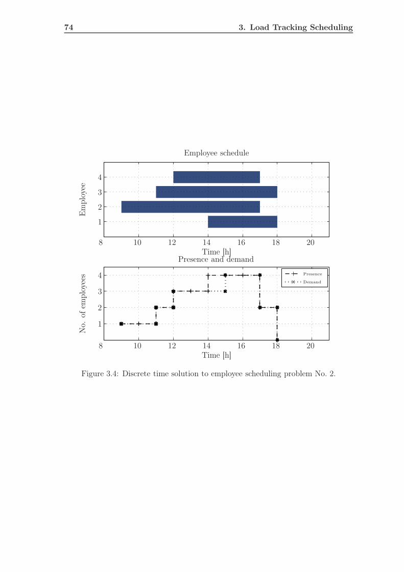
74 3. Load Tracking Scheduling
Employee schedule
Em
ploy
ee
Time [h]
No.
ofem
ploy
ees
Time [h]
Presence and demand
Presence
Demand
8 10 12 14 16 18 20
8 10 12 14 16 18 20
1
2
3
4
1
2
3
4
Figure 3.4: Discrete time solution to employee scheduling problem No. 2.
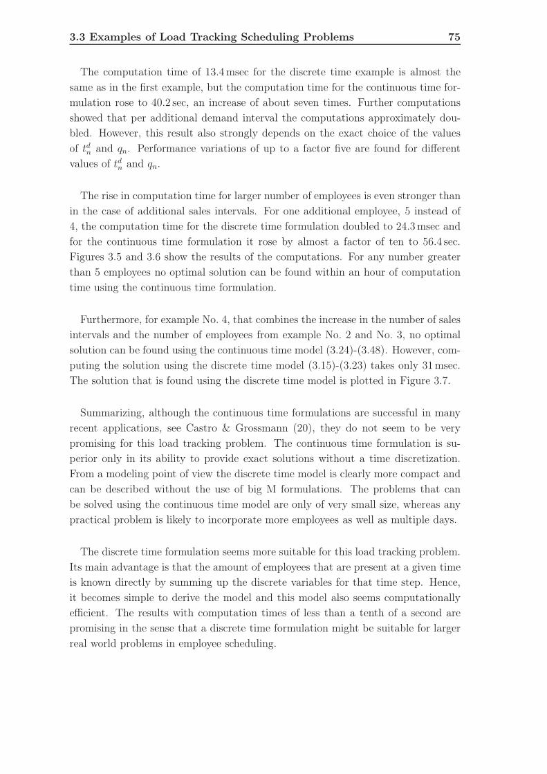
3.3 Examples of Load Tracking Scheduling Problems 75
The computation time of 13.4msec for the discrete time example is almost thesame as in the first example, but the computation time for the continuous time for-mulation rose to 40.2 sec, an increase of about seven times. Further computationsshowed that per additional demand interval the computations approximately dou-bled. However, this result also strongly depends on the exact choice of the valuesof tdn and qn. Performance variations of up to a factor five are found for differentvalues of tdn and qn.
The rise in computation time for larger number of employees is even stronger thanin the case of additional sales intervals. For one additional employee, 5 instead of4, the computation time for the discrete time formulation doubled to 24.3msec andfor the continuous time formulation it rose by almost a factor of ten to 56.4 sec.Figures 3.5 and 3.6 show the results of the computations. For any number greaterthan 5 employees no optimal solution can be found within an hour of computationtime using the continuous time formulation.
Furthermore, for example No. 4, that combines the increase in the number of salesintervals and the number of employees from example No. 2 and No. 3, no optimalsolution can be found using the continuous time model (3.24)-(3.48). However, com-puting the solution using the discrete time model (3.15)-(3.23) takes only 31msec.The solution that is found using the discrete time model is plotted in Figure 3.7.
Summarizing, although the continuous time formulations are successful in manyrecent applications, see Castro & Grossmann (20), they do not seem to be verypromising for this load tracking problem. The continuous time formulation is su-perior only in its ability to provide exact solutions without a time discretization.From a modeling point of view the discrete time model is clearly more compact andcan be described without the use of big M formulations. The problems that canbe solved using the continuous time model are only of very small size, whereas anypractical problem is likely to incorporate more employees as well as multiple days.
The discrete time formulation seems more suitable for this load tracking problem.Its main advantage is that the amount of employees that are present at a given timeis known directly by summing up the discrete variables for that time step. Hence,it becomes simple to derive the model and this model also seems computationallyefficient. The results with computation times of less than a tenth of a second arepromising in the sense that a discrete time formulation might be suitable for largerreal world problems in employee scheduling.
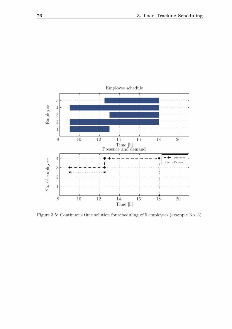
76 3. Load Tracking Scheduling
Employee schedule
Em
ploy
ee
Time [h]
No.
ofem
ploy
ees
Time [h]
Presence and demand
Presence
Demand
8 10 12 14 16 18 20
8 10 12 14 16 18 20
1
2
3
4
1
2
3
4
5
Figure 3.5: Continuous time solution for scheduling of 5 employees (example No. 3).

3.3 Examples of Load Tracking Scheduling Problems 77
Employee schedule
Em
ploy
ee
Time [h]
No.
ofem
ploy
ees
Time [h]
Presence and demand
Presence
Demand
8 10 12 14 16 18 20
8 10 12 14 16 18 20
1
2
3
4
1
2
3
4
5
Figure 3.6: Discrete time solution for scheduling of 5 employees (example No. 3).
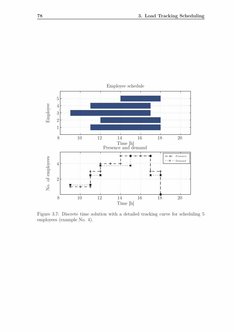
78 3. Load Tracking Scheduling
Employee schedule
Em
ploy
ee
Time [h]
No.
ofem
ploy
ees
Time [h]
Presence and demand
Presence
Demand
8 10 12 14 16 18 20
8 10 12 14 16 18 20
2
4
1
2
3
4
5
Figure 3.7: Discrete time solution with a detailed tracking curve for scheduling 5employees (example No. 4).

3.3 Examples of Load Tracking Scheduling Problems 79
3.3.2 Steel Manufacturing Problem
The second project considers optimization of the operation of a steel plant. Ageneral overview on optimization problems arising in steel manufacturing is givenin the survey paper of Dutta and Fourer Dutta & Fourer (29), while the paper ofTang et al. (61) reviews planning and scheduling methods that are actually used inthe industry.
In our analysis we focus on scheduling the material flow through the plant whichwould minimize the operating cost of the plant. The problem of cost optimal schedul-ing of the material flow has also been analyzed in Nystrom et al. (52), Pacciarelli &Pranzo (53), Tang et al. (60), Boukas et al. (12), Harjunkoski & Grossmann (38).The papers Boukas et al. (12) and Pacciarelli & Pranzo (53) focus on minimizingthe makespan and thus search for the shortest schedule to complete a given set oforders.
Papers Nystrom et al. (52) and Harjunkoski & Grossmann (38) present problemsthat involve multiple grades of steel that are manufactured in a single plant. Intheir optimization models, they minimize the cost of changeovers from one gradeof steel to another and the operation cost of the units. The paper Harjunkoski &Grossmann (38) accomplishes this by imposing a secondary optimization problemthat first groups similar steel grades in order to have minimal changeover cost withinthese groups. The paper of Tang et al. (60) presents a formulation for a just-in-timeproduction problem. In their formulation the cost arises due to either earlier ordelayed production of the just-in-time parts.
In contrast to the previous objectives reported in the literature, in the schedulingproblem here a load tracking objective is considered. The goal of the schedule is toarrange the material flow and production tasks so that the energy consumption ofthe entire plant deviates as little as possible from a pre-specified load curve.
The problem formulation and requirements are collected from an industry collab-oration project. In this project the steel plant is offered a rebate by the electricityprovider if it runs the plant such that the plants electricity demand over the daytracks a previously negotiated load curve. Deviations, overconsumption and under-consumption are penalized and thus should be avoided.
This situation reflects a typical load tracking problem as introduced in Section 3.2.The tasks of the manufacturing process need to be arranged such that a pre-specifiedcurve is tracked. A slight change to the general formulation is introduced by thefact that the electrical load of the plant is not measured continuously, but it is thecumulative load during each time interval which has to be matched to the requiredload.

80 3. Load Tracking Scheduling
A schematic view of the plant under consideration is shown in Figure 3.8. Thefigure shows five types of machines that can be found in the plant and indicatessome possible routes of the steel flow during the manufacturing process. The steel istransported in ladles from one unit to the next. The setup presented in Figure 3.8is proposed by industrial collaborators as a typical steel plant layout.
In the plant under consideration the ladles are moved by one crane. This craneis responsible for all transitions that are indicated by arcs. It is pointed out byan industrial collaborator that the crane movement is a potential bottleneck insystems operation and needs to be included explicitly as a resource into the problemformulation. Finally, the continuous casting machine (CCM) must run continuously.Thus, a fresh ladle of steel alway needs to be delivered to the casting machine whenthe previous one is about to be depleted.
3.3.2.1 Objective and Constraints
In the steel plant scheduling case, a list of tasks belonging to different processeshas to be arranged such that operational requirements are respected. These re-quirements include minimum and maximum processing times, capacity constraintsand the constraint that ensures uninterrupted operation of the continuous castingmachine. The crane must be modeled as a resource to avoid conflicts when shiftingladles from one machine to another.
The objective of the steel scheduling problem is to find a schedule such thatthe energy consumption of the plant tracks a pre-specified load curve as good aspossible. During the steel making process, each executed task imposes a certainelectrical load (power consumption). The current load of the plant is then given bythe sum of the instantaneous loads of all tasks. This current load is accumulatedover the interval specified by the load curve. The difference between the cumulatedand the pre-specified load is penalized, see Figure 3.9. The objective is to scheduleall tasks such that their schedule minimizes this penalty.
In summary, the requirements for the steel scheduling problem are:
1. Each scheduled task has to be processed at some time.
2. No task can be interrupted, i. e. they are non preemptive.
3. The order of the tasks within a manufacturing process is fixed and no idle timeduring the process is allowed.
4. Each machine can only run one task at a time.
5. Each task has a minimum processing time.

3.3 Examples of Load Tracking Scheduling Problems 81
LFEAF CCM
DS VD
Figure 3.8: Steel plant diagram.
elec
tric
load
15 min average loadpenalty
scheduled loadinstant load
15 min intervalltime
Figure 3.9: Illustration of Objective Function.

82 3. Load Tracking Scheduling
6. Each task has a maximum processing time.
7. The continuous casting machine is not allowed to have an idle time.
8. The crane can be used to change only one ladle at a time.
9. The objective is to minimize the difference between required and average actualenergy consumption during each load interval.
Discrete time and continuous time formulations for the steel problem are given inSections 3.3.2.2 and 3.3.2.3. To model the problem, the following indices and setsare used:
• Processes are indexed with j ∈ J , where J is the set of all processes. Aprocess states the sequence of tasks that need to be performed to manufactureone batch (here a ladle) of steel.
• Machines are indexed by i ∈ I, where I is the set of all machines, includingthe crane.
• All tasks are indexed with l ∈ L.
• The tasks running on machine i are given by set Li.
• The sequence of the tasks is stored in the set S that contains 2-tuples with allpairs of subsequent tasks (l′, l′′) ∈ S, where task l′ precedes task l′′.
• The pre-specified load curve consists of load intervals indexed by n ∈ N . Eachload interval is a 2-tuple given by (tdn, qn) ∈ E , with tdn being the starting timeand qn being the load of interval n. The intervals are ordered and cover theentire time horizon, thus the starting time tdn+1 of interval n + 1 is the endtime of interval n.
• The energy consumption of machine i is given by pi.
• The tracking error for each load interval is denoted by en.
3.3.2.2 Discrete Time Model
Two discrete time models are presented in this section. The first one is based onthe standard discrete time modeling approach as described in Section 3.2.1.1. Thesecond discrete time model is based on the requirements using propositional logic.This formulation can then be transformed into an MLD model using a compiler suchas HYSDEL, see Section 3.2.1.2.

3.3 Examples of Load Tracking Scheduling Problems 83
Discrete time model using linear inequalities
In discrete time models, the time variable is discretized at a uniform rate, TSample.The time horizon considered is then segmented with discrete time points t ∈ T ,where T = {1, . . . , T}. The work on a task l at time t is represented by the binaryvariable δl,t ∈ {0, 1}, where a value of one means that the task l is worked on attime t. The requirements stated in Section 3.3.2.1 are modeled as follows:
• Requirement 1: Summing all δl,t over all times t ensures that each task isscheduled at least once: ∑
t∈T
δl,t ≥ 1 ∀l ∈ L. (3.49)
• Requirement 2: To ensure that tasks are not interrupted, additional binaryvariables are defined. These mark the beginning and ending of a task: δon
l,t ∈
{0, 1} and δoffl,t ∈ {0, 1}. The values of the on- and off-variables are defined as
the starting and ending points of a task by:
δoffl,t+1 ≥ δl,t − δl,t+1 ∀l ∈ L, t ∈ 1, . . . , T − 1, (3.50)
δonl,t ≥ δl,t − δl,t−1 ∀l ∈ L, t ∈ 2, . . . , T , (3.51)
δoffl,T ≥ δl,T ∀l ∈ L (3.52)
andδonl,1 ≥ δl,1 ∀l ∈ L. (3.53)
For the tasks to be not interrupted, we require at most one start and one endof a task. Therefore, ∑
t∈T
δoffl,t ≤ 1 ∀l ∈ L (3.54)
and ∑
t∈T
δonl,t ≤ 1 ∀l ∈ L (3.55)
must hold. Note that introducing either δonl,t or δoff
l,t would have been sufficientfor Requirement 2, however both variables are needed later in the model.
• Requirement 3: To fix the order and have no idle time throughout the pro-cesses, we use the set of subsequent tasks (l′, l′′) ∈ S. For each of these pairsit must hold that the ending time of l′ is equal to the starting time of l′′:
∑
t∈T
t δoff
l′,t =∑
t∈T
t δonl′′,t ∀(l
′, l′′) ∈ S. (3.56)

84 3. Load Tracking Scheduling
• Requirement 4: Using the set Li of tasks running on machine i, we can confirmthat at most one task runs on that machine at a time by constraining:
∑
l∈Li
δl,t ≤ 1 ∀i ∈ I, t ∈ T . (3.57)
• Requirement 5: To ensure that the minimum processing durations are re-spected each task has a minimum active time T lmin
l . This minimum durationis met by constraining the number of time steps during which the task is activeto be larger than T lmin
l /Tsample:
∑
t∈T
δl,t ≥ T lminl /Tsample ∀l ∈ L. (3.58)
• Requirement 6: The maximum processing time T lmaxl can be ensured in an
analogous manner to Requirement 5:
∑
t∈T
δl,t ≤ T lmaxl /Tsample ∀l ∈ L. (3.59)
• Requirement 7: To fulfill the continuous casting machine (CCM) requirement,we require the on and off times of tasks on the CCM to be adjacent:
∑
l∈Li
δoffl,t −
∑
l∈Li
δonl,t+1 ≤ 0 i = ”ccm”, ∀t ∈ {1, . . . , T − 1}. (3.60)
• Requirement 8: The requirement is covered by the machine requirements thatallow only one machine use at a time and have a minimum time requirement.
• Requirement 9 (Objective): Using the specified load curve (tdn, qn) ∈ E , we canmodel the tracking error en by
en ≥ −qn +∑
i∈I
∑
l∈Li
tdn+1∑
t=tdn
pi δl,t ∀n ∈ N (3.61)
and
en ≥ qn −∑
i∈I
∑
l∈Li
tdn+1∑
t=tdn
pi δl,t ∀n ∈ N . (3.62)

3.3 Examples of Load Tracking Scheduling Problems 85
The objective is then to minimize the tracking error:
min∑
n∈N
en. (3.63)
The model equations (3.49) -(3.63) fulfill all requirements that are requested by theindustrial collaborator. However, the model is clearly a simplified version of whatis needed to fully model a scheduling system for steel manufacturing. Most likelya more realistic version would require constraints that allow operators to influencethe schedule directly by blocking machines i or assigning tasks l to be performed ona machine at a specific time t. Using the discrete time framework such constraintsare simple to implement. They are assignments of zero or one to the δl,t variablesthat model the work on task l at time t.
Discrete time model using logic rules
The concept of using propositional logic for the formulation of a scheduling problemwas introduced in Gallestey et al. (36) and is described in Section 3.2.1.2. A for-mulation in logic can later be translated into a MLD system which can be treatedusing tools from control engineering, for an example see Kvasnica & Baotić (43).
To model logic rules so that they can be automatically compiled into MLD form,some additional variables are introduced. A state variable xm
j (t) ∈ I determines, fortime t and process j, the machine number i ∈ I on which the process is currentlyactive. In addition, the steps of process j are given by a sequence sj,k with k ∈
{1, . . . , |K|} elements; the first element sj,1 points to the electric arc furnace whereall processes start and the last element sj,|K| points to the continuous casting machine(CCM) that marks the last step of each process. The state in the sequence is denotedby xs
j ∈ K for process j.
To model processing times we associate each process j and machine i combinationwith a timer variable xt
i,j(t) that records the duration, which a process has beenactive at time t. In this model, the continuous casting machine is fed by a tank,and ladles from different processes may be mixed in the tank. This is a slightsimplification compared to the other models and may or may not apply in practice.The filling level of the continuous casting machine is denoted by xccm(t) and isconstrained to be within xccm
min and xccmmax. If the constraints xccm
min and xccmmax are set to
zero then this model will be the same as the other models. The system inputs areswitching signals uj(t) ∈ {0, 1} and the outflow of the continuous casting machineuout(t).

86 3. Load Tracking Scheduling
The model is constructed by formulating the equations that fulfill the requirementsgiven in Section 3.3.2.1:
• Requirements 1, 2 and 3 can be modeled by constraining all elements in thetask sequence to take place in the correct order. Thus, if the switching signaluj for process j is equal to one then the process switches to the next machinein its processing sequence sj,k. If the switching signal is zero nothing changes.
uj(t) = 0 ⇒ xsj(t + 1) = sj,k+1 ∀j ∈ J , t ∈ T , (3.64)
uj(t) = 1 ⇒ xsj(t + 1) = xs
j(t) ∀j ∈ J , t ∈ T . (3.65)
• Requirements 4 and 8 are modeled using binary variables δi,j(t) that indicatethe use of machine i by process j at time t:
xj(t) = i ⇒ δi,j(t) = 1 ∀i ∈ I, j ∈ J , t ∈ T , (3.66)
xj(t) 6= i ⇒ δi,j(t) = 0 ∀i ∈ I, j ∈ J , t ∈ T ; (3.67)
at most one process can run on machine i at a time
∑
j∈J
δi,j(t) ≤ 1 ∀i ∈ I, t ∈ T . (3.68)
• Requirement 5 disallows a switching signal uj to switch to the next task if theminimum task time is not fulfilled:
xti,j(t) < Tmin
i,j ⇒ uj(t) = 0 ∀i ∈ I, j ∈ J , t ∈ T . (3.69)
In order to check the runtime of a task, the timer xti,j is introduced and in-
creased while process j runs on machine i:
δi,j(t) = 1 ⇒ xti,j(t + 1) = xt
i,j(t) + 1 ∀i ∈ I, j ∈ J , t ∈ T , (3.70)
δi,j(t) = 0 ⇒ xti,j(t + 1) = 0 ∀i ∈ I, j ∈ J , t ∈ T . (3.71)
• Requirement 6 constrains the maximum processing time and bounds the timerxt
i,j of process j on machine i:
xti,j(t) ≤ Tmax
i,j ∀i ∈ I, j ∈ J , t ∈ T . (3.72)
• Requirement 7 ensures continuous casting by constraining the reservoir of the

3.3 Examples of Load Tracking Scheduling Problems 87
casting machine to never run empty. The reservoir filling level is given byxccm(t). The inflow to the reservoir is given by the ladle volume Vj for processj and the casting outflow by the input variable uout
y (t):
xccm(t + 1) = xccm(t) + uin(t)− uout(t) ∀t ∈ T , (3.73)
xsj(t) = |Kj| − 1 ∧ uj(t) = 1 ⇒ uin(t) = Vj ∀t ∈ T , (3.74)
xsj(t) 6= |Kj | − 1 ∨ uj(t) 6= 1 ⇒ uin(t) = 0 ∀t ∈ T , (3.75)
uoutmin ≤ uout(t) ≤ uout
max ∀t ∈ T , (3.76)
xccmmin ≤ xccm(t) ≤ xccm
max. (3.77)
• Requirement 8: The cost function is almost identical to the one in the previ-ously presented discrete time model. Using the specified load curve (tsn, qn) ∈
E , we can model the tracking error en by:
en ≥ −qn +∑
i∈I
∑
j∈J
tdn+1∑
t=tsn
pi δi,j(t) ∀n ∈ N (3.78)
and
en ≥ qn −∑
i∈I
∑
l∈J
tdn+1∑
t=tdn
pi δi,j(t) ∀n ∈ N . (3.79)
The optimal schedule is obtained by minimizing
min∑
n∈N
en. (3.80)
3.3.2.3 Continuous Time
For the continuous time model we assign to each task l a starting and ending timetsl and tel . The model is constructed by modeling all requirements posed in Sec-tion 3.3.2.1:
• Requirement 1. All starting and ending times are assigned within the timehorizon T :
tsl , tel ∈ T . (3.81)
• Requirement 2. The tasks are not interrupted since only one start and endpoints per task exist.

88 3. Load Tracking Scheduling
• Requirement 3. Using the sequence set S, the requirement is satisfied byrequiring the ending time tel′ of the preceding task l′ to be equal to the startingtime tsl′′ of the subsequent task l′′:
tel′ = tsl′′ ∀(l′, l′′) ∈ S. (3.82)
• Requirement 4. Using the set of all tasks l1, l2 ∈ Li that run on machine i, weensure that the starting time tsl1 of each task is either after the end of tel2 ortsl2 is after tel1 . To model the or-relationship, we use a binary variable δl1,l2andthe big M technique:
tel1 ≤ tsl2 + M(1− δl1,l2) ∀l1, l2 ∈ {l1, l2 : l1, l2 ∈ Li, l1 < l2}, i ∈ I, (3.83)
tel12 ≤ tsl1 + M δl1,l2 ∀l1, l2 ∈ {l1, l2 : l1, l2 ∈ Li, l1 < l2}, i ∈ I. (3.84)
• Requirement 5. The minimum processing time T lminl is ensured by requiring:
tel − tsl ≥ T lminl ∀l ∈ L. (3.85)
• Requirement 6. The maximum processing time T lmaxl is ensured by requiring:
tel − tsl ≤ T lmaxl ∀l ∈ L. (3.86)
• Requirement 7. The continuous casting requirement is modeled by requiringthat for every task l1 running on the continuous casting machine there existsa second task l2 on the CCM for which the starting point tsl2 is equal to theendpoint tel1of task l1:
tel1 ≤ tsl2 + M(1− δccml1,l2
) ∀l1, l2 ∈ Lccm, (3.87)
tsl2 ≤ tel1 + M(1− δccml1,l2
) ∀l1, l2 ∈ Lccm, (3.88)∑
l2∈Lccm
δccml1,l2
= 1 ∀l1 ∈ Lccm. (3.89)
• Requirement 8: The crane requirement is fulfilled through the machine re-quirements No. 2 and No. 4 that allow only one use at a time.
• Requirement 9 (Objective): To model the objective, additional constraints arerequired. These compute the energy consumption within each load interval.

3.3 Examples of Load Tracking Scheduling Problems 89
For each load interval task combination, there exist six possible cases how theintervals may lie with respect to each other. The task may take place:
1. before the load interval,
2. start before and end within the load interval,
3. start and end within the load interval,
4. start before and end after the load interval,
5. start within and end after the load interval,
6. takes place after the load interval.
The possible cases are illustrated in Figure 3.10. Using big M technique, toeach case integer variables δload1
l,n to δload6l,n are assigned. The energy consumption
that task l contributes to the load requirement of load interval n is given bywl,n. The contributions are computed in a two step approach. First the typeof overlap is determined and then the appropriate contribution to the loadrequirement is added.
Case 1: If the task l takes place before the load interval n, it holds that
tel ≤ tdn + M(1− δload1l,n ) ∀l ∈ L, n ∈ N (3.90)
and the contribution wl,n is computed by
wl,n ≤ M(1− δload1l,n ) ∀l ∈ L, n ∈ N . (3.91)
Case 2: If the task l begins before and ends inside the load interval n, it holdsthat
tsl ≤ tdn + M(1− δload2l,n ) ∀l ∈ L, n ∈ N , (3.92)
tel > tdn −M(1− δload2l,n ) ∀l ∈ L, n ∈ N , (3.93)
tel < tdn+1 + M(1− δload2l,n ) ∀l ∈ L, n ∈ N , (3.94)
and for the load contribution:
wl,n ≤ pi (tel − tdn) + M(1− δload2
l,n ) ∀l ∈ Li, n ∈ N , i ∈ I, (3.95)
wl,n ≥ pi (tel − tdn)−M(1− δload2
l,n ) ∀l ∈ Li, n ∈ N , i ∈ I. (3.96)
Case 3: When the task takes place entirely inside the load interval, it holdsthat

90 3. Load Tracking Scheduling
1.
2.
3.
4.
5.
6.
case:
load interval overlap:
task:
Figure 3.10: Six possible classes of load interval overlap.
tsl ≥ tdn −M(1− δload3l,n ) ∀l ∈ L, n ∈ N , (3.97)
tel ≤ tdn+1 + M(1− δload3l,n ) ∀l ∈ L, n ∈ N , (3.98)
and for the load contribution:
wl,n ≤ pi (tel − tsl ) + M(1− δload3
l,n ) ∀l ∈ Li, n ∈ N , i ∈ I, (3.99)
wl,n ≥ pi (tel − tsl )−M(1− δload3
l,n ) ∀l ∈ Li, n ∈ N , i ∈ I. (3.100)
Case 4: Tasks starting before and ending after the load interval n:
tsl < tdn + M(1− δload4l,n ) ∀l ∈ L, n ∈ N , (3.101)
tel > tdn+1 −M(1− δload4l,n ) ∀l ∈ L, n ∈ N , (3.102)
and for the load contribution:
wl,n ≤ pi (tdn − tdn+1) + M(1− δload4
l,n ) ∀l ∈ Li, n ∈ N , i ∈ I, (3.103)
wl,n ≥ pi (tdn − tdn+1)−M(1− δload4
l,n ) ∀l ∈ Li, n ∈ N , i ∈ I. (3.104)

3.3 Examples of Load Tracking Scheduling Problems 91
Case 5: If the task l starts within and ends after the load interval n:
tsl > tdn −M(1− δload5l,n ) ∀l ∈ L, n ∈ N , (3.105)
tel < tdn + M(1− δload5l,n ) ∀l ∈ L, n ∈ N , (3.106)
tel ≥ tdn+1 −M(1− δload5l,n ) ∀l ∈ L, n ∈ N (3.107)
and for the load contribution:
wl,n ≤ pi (tdn+1 − tsl ) + M(1− δload5
l,n ) ∀l ∈ Li, n ∈ N , i ∈ I, (3.108)
wl,n ≥ pi (tdn+1 − tsl )−M(1− δload5
l,n ) ∀l ∈ Li, n ∈ N , i ∈ I. (3.109)
Case 6: If the load interval n is entirely before task l takes place, it holds
tsl ≥ tdn+1 −M(1− δload6l,n ) ∀l ∈ L, n ∈ N (3.110)
and thenwl,n ≤ M(1− δload6
l,n ) ∀l ∈ L, n ∈ N . (3.111)
Since only one case can be active the binary variables are constrained:
δload1l,n + δload2
l,n + δload3l,n + δload4
l,n + δload5l,n + δload6
l,n = 1 ∀l ∈ L, n ∈ N . (3.112)
Using the load contributions wl,n from all tasks l to the load interval n, thetracking error en per load interval n is given by
en ≥ −qn +∑
l∈L
wl,n ∀n ∈ N (3.113)
for positive deviations and
en ≥ qn −∑
l∈L
wl,n ∀n ∈ N (3.114)
for negative deviations.
Then the objective function becomes
min∑
n∈N
en . (3.115)

92 3. Load Tracking Scheduling
3.3.2.4 Comparison of Models and Analysis
This section will analyze the performance of implementations of the models fromSection 3.3.2.2 and 3.3.2.3. The continuous time and the discrete time formulationsof the steel problem are implemented. However, the implementation of the formu-lation based on propositional logic is omitted since the MILP constraints that aregenerated with a compiler do not seem as compact as in the discrete time model.Therefore, no performance gain of the propositional logic formulation is expectedover the general discrete time model. Furthermore, no efficient compiler exists thatcan interpret a formulation with vectors of decision variables as it is presented inthe model (3.64)-(3.80). The current version of HYSDEL can only interpret one di-mensional variables, which would make the implementation and testing for differentproblem sizes very time consuming, see Torrisi et al. (64).
The constraints and objective of the discrete time scheduling model (3.49)-(3.63)and the continuous time model (3.81)-(3.115) are implemented in Matlab and passedto Cplex for solving Cplex (25).
To evaluate the models, five units are considered: the Electric Arc Furnace (EAF),the Ladle Furnaces (LF), the Deslagging Unit (DS), the Continuous Casting Machine(CCM) and the Crane (C). In operation the units consume different amounts ofenergy. The energy consumptions per unit are given in Table 3.3. The values areestimated by talking to the industrial collaborator.
The time horizon given by T is constrained to be the end of the last interval ofthe specified load curve. In the discrete and continuous time models, the continuouscasting constraint cannot be fulfilled until the first casting is started on the CCM.Hence, to avoid a violation of the constraints (3.60) or (3.87)-(3.89), a virtual taskis included that runs from time 0 until the first casting process starts. The virtualcasting task produces zero load and is not explicitly listed for the examples. In thediscrete time model, a one minute time discretization is used, i. e. Tsample = 1 min.According to the industrial collaborator one minute represents the current planningtime interval for crane movements. Since it is a requirement to model the craneusage accurately it is not possible to chose a longer discretization interval.
In the following analysis, computation times do not consider the construction ofthe matrices, but only the runtime of the optimizer Cplex. Instances of the problemare solved for different task and load curve values to compare the performancesof the discrete and continuous time models and demonstrate their computationallimits.
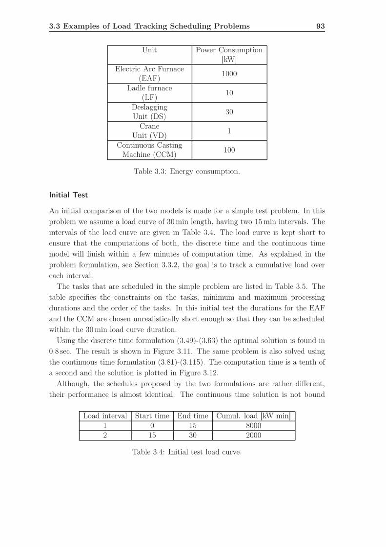
3.3 Examples of Load Tracking Scheduling Problems 93
Unit Power Consumption[kW]
Electric Arc Furnace(EAF)
1000
Ladle furnace(LF)
10
DeslaggingUnit (DS)
30
CraneUnit (VD)
1
Continuous CastingMachine (CCM)
100
Table 3.3: Energy consumption.
Initial Test
An initial comparison of the two models is made for a simple test problem. In thisproblem we assume a load curve of 30min length, having two 15min intervals. Theintervals of the load curve are given in Table 3.4. The load curve is kept short toensure that the computations of both, the discrete time and the continuous timemodel will finish within a few minutes of computation time. As explained in theproblem formulation, see Section 3.3.2, the goal is to track a cumulative load overeach interval.
The tasks that are scheduled in the simple problem are listed in Table 3.5. Thetable specifies the constraints on the tasks, minimum and maximum processingdurations and the order of the tasks. In this initial test the durations for the EAFand the CCM are chosen unrealistically short enough so that they can be scheduledwithin the 30min load curve duration.
Using the discrete time formulation (3.49)-(3.63) the optimal solution is found in0.8 sec. The result is shown in Figure 3.11. The same problem is also solved usingthe continuous time formulation (3.81)-(3.115). The computation time is a tenth ofa second and the solution is plotted in Figure 3.12.
Although, the schedules proposed by the two formulations are rather different,their performance is almost identical. The continuous time solution is not bound
Load interval Start time End time Cumul. load [kW min]1 0 15 80002 15 30 2000
Table 3.4: Initial test load curve.

94 3. Load Tracking Scheduling
CC
M
CC
M
CEA
F
EA
F
C
Time [min]
Pro
cess
ID
Gantt Chart
Time [min]
Pow
erC
onsu
mpt
ion
[kW
]
Load Curve Tracking, tracking error: 1.5 kWmin
scheduled
instant
interval accum.
0 5 10 15 20 25 30
0 5 10 15 20 25 30
0
200
400
600
800
1000
1200
1
2
Figure 3.11: Discrete time solution of the initial test scheduling problem.

3.3 Examples of Load Tracking Scheduling Problems 95
CC
M
CC
M
CEA
F
EA
F
C
Time [min]
Pro
cess
ID
Gantt Chart
Time [min]
Pow
erC
onsu
mpt
ion
[kW
]
Load Curve Tracking, tracking error: 1.133 kWmin
scheduled
instant
interval accum.
0 5 10 15 20 25 30
0 5 10 15 20 25 30
0
200
400
600
800
1000
1200
1
2
Figure 3.12: Continuous time solution of the initial scheduling problem.

96 3. Load Tracking Scheduling
Task Process Unit Duration NextNo. No. min max Task1 1 EAF 4 6 22 1 C 3 6 33 1 CCM 4 64 2 EAF 4 6 55 2 C 3 6 66 2 CCM 4 6
Table 3.5: Task list for the initial test.
to a time discretization and starts some tasks at non-integer times to accomplishan even better result. However, due to the fine time discretization of 1min, theperformance gain of using a continuous time formulation compared to the discretetime version is small. On the other hand the computation time for this small exampleis eight times longer for the discrete time problem. A second test case using realistictask durations will show this effect more clearly.
Realistic Test
In a second test, the task durations are chosen to match durations that are suggestedby a collaborator from industry. The tasks to be scheduled are given with their pa-rameters in Table 3.7. The tasks represent a scheduling problem for three batches ofsteel. The schedule is supposed to track the load curve that is specified in Table 3.6.The load curve is chosen based on a rough estimate of what the energy consump-tion for the production schedule might be. This method of generating a load curvemight be similar to what is used in practice, where the operator estimates his en-ergy demands and sends his estimates a few days ahead to the electricity provider.The optimal scheduling is then done only shortly before the ordered energy getsconsumed.
Using the continuous time formulation, a first feasible schedule is found withinless than a second. Computing the optimal schedule takes 3.3 sec. The solutionis plotted in Figure 3.13. The discrete time approach fails to even find a feasiblesolution within 12 hours.
For the steel plant scheduling problem, the continuous time formulation seems tobe by far superior to the discrete time version. Compared to the employee schedulingproblem, this might appear surprising. However, when comparing the discrete timeformulations for the employee and the steel scheduling problems, it is found thatthe scheduling horizon in the steel problem is much longer. Here the steel problemconsiders 75 time steps, whereas the employee problem has only ten time steps.

3.3 Examples of Load Tracking Scheduling Problems 97
Load interval Start time End time Cumul. load [kWh]1 1 15 140002 15 30 150003 30 45 140004 45 60 90005 60 75 20006 75 90 8007 90 105 200
Table 3.6: Load curve for the realistic test example.
Task Process Unit Duration nextNo. No. min max Task1 1 EAF 16 20 22 1 C 3 6 33 1 DS 12 17 44 1 C 3 6 55 1 LF 14 18 66 1 C 3 6 77 1 CCM 18 228 2 EAF 20 26 99 2 C 3 6 1010 2 DS 8 12 1111 2 C 3 6 1212 2 LF 9 12 1313 2 C 3 6 1414 2 CCM 17 2315 3 EAF 16 17 1616 3 C 3 6 1717 3 DS 6 8 1818 3 C 3 6 1919 3 CCM 20 24
Table 3.7: Task list for the realistic test.

98 3. Load Tracking Scheduling
Choosing a different time discretization with longer intervals is not an option sinceit does not allow the detailed crane scheduling that is requested by the collaborator.
Furthermore, in the employee scheduling problem, a binary variable is introducedper employee per time step. In the steel manufacturing problem each task is assigneda binary variable per time step. Already short manufacturing processes for one steelladle have at least five tasks. These factors increase the computation times of thediscrete time formulation of the steel manufacturing problem.
In contrast, the continuous time formulation appears to be much faster in the steelmanufacturing problem. However, in contrast to the employee scheduling problem,the sequence of the tasks is almost fixed. Within one process they must follow agiven sequence and only the processes may vary in their sequence. In the employeescheduling problem this is not the case as there is no constraint on which employeestarts first, second, and so on. For the continuous time formulation, finding theright sequence is a main source of complexity. Once the sequence is known binaryvariables in big M formulations, modeling the order in which task l′ and l′′ occuras specified by constraints (3.83)-(3.84), are fixed. This elimination simplifies theremaining problem.
Finally, for the steel problem, the objective requires that the cumulative loadper interval is tracked, whereas in the employee problem the objective is on trackingthe instantaneous load. Tracking the cumulative load means that only one deviationper load interval is computed, whereas in the employee scheduling case the deviationper event (starting and ending times of employee shifts and load intervals) must becomputed. The advantage of the discrete time model to have explicit informationon the instantaneous load is not needed in the steel case example. Altogether thismakes the continuous time model favorable for the steel scheduling problem.
Variations of Permissible Task Duration
To further explore the properties of the continuous time solution, we compute sched-ules for the task lists given in Table 3.8 and Table 3.9 and the load curve specifiedin Table 3.10. The difference between the two task lists is that the permissible taskdurations are extended to be one minute shorter or longer. All other parametersremain the same.
Solving the problem with the tighter bounds on the task durations takes 73.3 sec.The solution is plotted in Figure 3.14. For the slightly relaxed problem it takes7583.1 sec, which is more than 100 times longer. The solution to the relaxed problemis plotted in Figure 3.15.

3.3 Examples of Load Tracking Scheduling Problems 99
EA
F
C DS
C LF
C CC
M
EA
F
C DS
C LF
C CC
M
EA
F
C DS
C CC
M
Time [min]
Pro
cess
ID
Gantt Chart
Time [min]
Pow
erC
onsu
mpt
ion
[kW
]
Load Curve Tracking, tracking error: 204.12 kWmin
scheduled
instant
interval accum.
0 10 20 30 40 50 60 70 80 90 100
0 10 20 30 40 50 60 70 80 90 100
0
200
400
600
800
1000
1200
1
2
3
Figure 3.13: Continuous time solution of the realistic test problem.

100 3. Load Tracking Scheduling
Task Process Unit Duration NextNo. No. min max Task1 1 EAF 19 21 22 1 C 3 6 33 1 LF 6 8 44 1 C 3 6 55 1 DS 6 8 66 1 C 3 6 77 1 CCM 18 218 2 EAF 15 17 99 2 C 3 6 1010 2 LF 6 8 1111 2 C 3 6 1212 2 CCM 21 2413 3 EAF 16 18 1414 3 C 3 6 1515 3 LF 6 8 1616 3 C 3 6 1717 3 DS 6 8 1818 3 C 3 6 1919 3 CCM 18 21
Table 3.8: Task list for parameter variation test with tight min-/max task durations.

3.3 Examples of Load Tracking Scheduling Problems 101
Task Process Unit Duration NextNo. No. min max Task1 1 EAF 18 22 22 1 C 2 7 33 1 LF 5 9 44 1 C 2 7 55 1 DS 5 9 66 1 C 2 7 77 1 CCM 17 228 2 EAF 14 18 99 2 C 2 7 1010 2 LF 5 9 1111 2 C 2 7 1212 2 CCM 20 2513 3 EAF 15 19 1414 3 C 2 7 1515 3 LF 5 9 1616 3 C 2 7 1717 3 DS 5 9 1818 3 C 2 7 1919 3 CCM 17 21
Table 3.9: Task list for parameter variation test with relaxed min-/max task dura-tions.

102 3. Load Tracking Scheduling
Task Process Unit Duration NextNo. No. min max Task1 1 EAF 19 21 22 1 C 3 6 33 1 LF 6 8 44 1 C 3 6 55 1 DS 6 8 66 1 C 3 6 77 1 CCM 18 218 2 EAF 15 17 99 2 C 3 6 1010 2 LF 6 8 1111 2 C 3 6 1212 2 CCM 21 2413 3 EAF 16 18 1414 3 C 3 6 1515 3 LF 6 8 1616 3 C 3 6 1717 3 DS 6 8 1818 3 C 3 6 1919 3 CCM 18 21
Table 3.10: Task list for parameter variation test with tight min-/max task dura-tions.

3.3 Examples of Load Tracking Scheduling Problems 103
LF
CEA
F
C DS
C CC
M
EA
F
C LF
C CC
M
EA
F
C LF
C DS
C CC
M
Time [min]
Pro
cess
ID
Gantt Chart
Time [min]
Pow
erC
onsu
mpt
ion
[kW
]
Load Curve Tracking, tracking error: 351.35 kWmin
scheduled
instant
interval accum.
0 20 40 60 80 100 120
0 20 40 60 80 100 120
0
200
400
600
800
1000
1200
1
2
3
Figure 3.14: Solution with tighter min-/max task durations.

104 3. Load Tracking Scheduling
CEA
F
LF
C DS
C CC
M
EA
F
C LF
C CC
M
EA
F
C LF
C DS
C CC
M
Time [min]
Pro
cess
ID
Gantt Chart
Time [min]
Pow
erC
onsu
mpt
ion
[kW
]
Load Curve Tracking, tracking error: 269.1 kWmin
scheduled
instant
interval accum.
0 20 40 60 80 100 120
0 20 40 60 80 100 120
0
200
400
600
800
1000
1200
1
2
3
Figure 3.15: Solution with relaxed min-/max task durations.

3.3 Examples of Load Tracking Scheduling Problems 105
The effect of this small change in the permissible task durations is rather sur-prising, especially since the two optimization problems have the same number ofvariables and constraints. Hence, the enlarged solution space is the source of theincreased computation time.
Both problems are also solved by setting the objective to be zero. Thus the solveronly searches for a feasible solution. In both cases this solution is found in about atenth of a second. Therefore, the longer computation time is not due to finding afeasible solution, but must be due to the objective function.
We argue that the increased flexibility allows for more possible task load intervaloverlaps, since the start or end times may fall into different load intervals, see Fig-ure 3.16. Thus, a task that in the inflexible situation could only finish in one loadinterval can now end in several different load intervals. Solving for the end time ifa task is known to finish in a specific interval means solving a pure linear program,but if there are more possible task-load overlaps these are modeled using the big Mformulation, see Equations (3.90)-(3.112). The number of possible overlaps increasesthe number of possible integer combinations in the optimization problem that needto be searched and this results in a longer computation time.
For possible application projects, this increase demonstrates that the effectivenessof a solution algorithm does not only depend on the size of the problem, i. e. thenumber of variables it contains. It also depends on the values of the parameters inthe problem. Often the values may not be known exactly before the implementationand thus this example underlines the importance of thorough testing.
Moreover, it implies for a second conclusion. By artificially fixing parts or thewhole sequence or just reducing the flexibility, the scheduling optimization problemis simplified. Thus the amount of flexibility or the amount of fixing of a sequencebecome potential tuning parameters in real world problems.
15 min interval
flexible task
inflexible task possibleend time
time
Figure 3.16: Flexible tasks enlarge the search tree by adding new cases.

106 3. Load Tracking Scheduling
Online scheduling
In the previous examples the focus was on solving the scheduling problems to op-timality. Although achieving an optimal solution is desirable, it is usually not nec-essary or practical in real applications. For example, in the case with flexible taskdurations, see Table 3.9 and Figure 3.15, computing the solution for a 2 hour timeperiod takes longer than 2 hours. Hence, applying the algorithm to find optimalsolutions may not be possible.
Moreover, in practical applications a “good” solution will often be sufficient. MILPsolvers produce feasible but suboptimal solutions during their solution process.These solutions can be queried, or the solution process can be stopped at a cer-tain time and the best solution obtained so far is retrieved. In this example wecompute a solution for a 4 hour time horizon and the solver is given a computationtime of 1min. The load curve parameters for this example are given in Table 3.11and the task parameters are listed in Table 3.12. The values in Table 3.11 and 3.12are estimated based on comments from the collaborator on what a realistic casemight require. The obtained solution is plotted in Figure 3.17. Note that thissolution already fulfills all the constraints. In particular, feasible crane schedulesand schedules ensuring continuous casting are obtained. Both of these features aredifficult to obtain by manually arranging the tasks.
Thus, stopping the optimization prematurely may also be a feasible tuning ap-proach for real world applications. However, once again it must be determinedfrom the application whether the sub-optimal solutions that are obtained are goodenough.
3.4 Conclusions
In this paper we compare continuous and discrete time models for load trackingscheduling problems. Two application examples are chosen for this comparison.One is a problem for demand driven employee shift scheduling and the second isthe energy cost optimal scheduling of a steel plant. Both problems are simplifiedversions of real application problems. Each problem is formulated in a continuousand a discrete time scheduling framework. In both cases the discrete time model ismore intuitive to construct since it models the resource and task activity at each timepoint explicitly by a variable. In the continuous time model, the task activity hasto be inferred by comparing the starting and ending times, which leads to either-ortype of conditions. Such conditions require big M constraints and are more complexin the sense that they require the modeler to think in terms of a set of different cases

3.4 Conclusions 107
EA
F
C LF
C DS
C CC
ME
AF
C LF
C CC
M
EA
F
C LF
C DS
C CC
M
EA
FC D
SC C
CM
EA
F
C DS
C LF
C CC
M
EA
F
C DS
C CC
M
Time [min]
Pro
cess
ID
Gantt Chart
Time [min]
Pow
erC
onsu
mpt
ion
[kW
]
Load Curve Tracking, tracking error: 7304.93 kWmin
scheduled
instant
interval accum.
0 50 100 150 200 250
0 50 100 150 200 250
0
200
400
600
800
1000
1200
1
2
3
4
5
6
Figure 3.17: Sub-optimal solution for a 4 hour schedule.
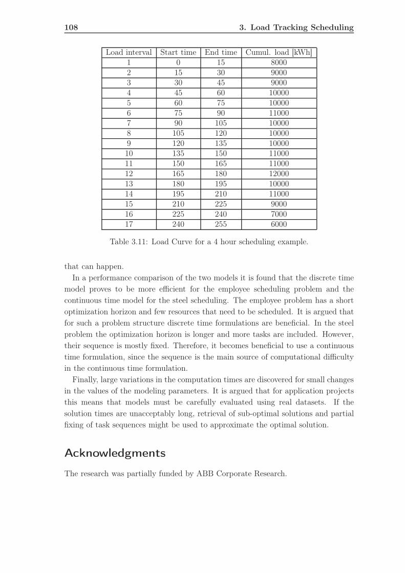
108 3. Load Tracking Scheduling
Load interval Start time End time Cumul. load [kWh]1 0 15 80002 15 30 90003 30 45 90004 45 60 100005 60 75 100006 75 90 110007 90 105 100008 105 120 100009 120 135 1000010 135 150 1100011 150 165 1100012 165 180 1200013 180 195 1000014 195 210 1100015 210 225 900016 225 240 700017 240 255 6000
Table 3.11: Load Curve for a 4 hour scheduling example.
that can happen.In a performance comparison of the two models it is found that the discrete time
model proves to be more efficient for the employee scheduling problem and thecontinuous time model for the steel scheduling. The employee problem has a shortoptimization horizon and few resources that need to be scheduled. It is argued thatfor such a problem structure discrete time formulations are beneficial. In the steelproblem the optimization horizon is longer and more tasks are included. However,their sequence is mostly fixed. Therefore, it becomes beneficial to use a continuoustime formulation, since the sequence is the main source of computational difficultyin the continuous time formulation.
Finally, large variations in the computation times are discovered for small changesin the values of the modeling parameters. It is argued that for application projectsthis means that models must be carefully evaluated using real datasets. If thesolution times are unacceptably long, retrieval of sub-optimal solutions and partialfixing of task sequences might be used to approximate the optimal solution.
Acknowledgments
The research was partially funded by ABB Corporate Research.

3.4 Conclusions 109
Task Process Unit Duration NextNo. No. min max Task1 1 EAF 25 34 22 1 C 3 6 33 1 LF 14 17 44 1 C 3 6 55 1 DS 13 17 66 1 C 3 6 77 1 CCM 28 338 2 EAF 24 29 99 2 C 3 6 1010 2 LF 10 12 1111 2 C 3 6 1212 2 CCM 24 2913 3 EAF 22 27 1414 3 C 3 6 1515 3 LF 9 14 1616 3 C 3 6 1717 3 DS 16 19 1818 3 C 3 6 1919 3 CCM 22 2820 4 EAF 18 19 2121 4 C 3 6 2222 4 DS 10 13 2323 4 C 3 6 2424 4 CCM 20 2425 5 EAF 25 34 2626 5 C 3 6 2727 5 DS 14 17 2828 5 C 3 6 2929 5 LF 13 17 3030 5 C 3 6 3131 5 CCM 28 3332 6 EAF 24 29 3333 6 C 3 6 3434 6 DS 10 12 3535 6 C 3 6 3636 6 CCM 24 29
Table 3.12: Task list for 4 hour scheduling test.

110 Bibliography
Bibliography
[1] Addou, I. & Soumis, F. (2007). Bechtold-jacobs generalized model for shiftscheduling with extraordinary overlap. Annals of Operations Research, 155(1),177–205.
[2] Aickelin, U. & Li, J. (2007). An estimation of distribution algorithm for nursescheduling. Annals of Operations Research, 155(1), 289–309.
[3] Al-Yakoob, S. & Sherali, H. (2007). Mixed-integer programming models for anemployee scheduling problem with multiple shifts and work locations. Annals of
Operations Research, 155(1), 119–142.
[4] Ashford, R. (2007). Mixed integer programming: A historical perspective withxpress-mp. Annals of Operations Research, 149(1), 5–17.
[5] Bard, J., Morton, D., & Wang, Y. (2007). Workforce planning at usps mailprocessing and distribution centers using stochastic optimization. Annals of Op-
erations Research, 155(1), 51–78.
[6] Bard, J. F. & Purnomo, H. W. (2005). Preference scheduling for nurses usingcolumn generation. European Journal of Operational Research, 164(2), 510–534.
[7] Belien, J. & Demeulemeester, E. (2006). Scheduling trainees at a hospital de-partment using a branch-and-price approach. European Journal of Operational
Research, 175(1), 258–278.
[8] Belien, J. & Demeulemeester, E. (2007). On the trade-off between staff-decomposed and activity-decomposed column generation for a staff schedulingproblem. Annals of Operations Research, 155(1), 143–166.
[9] Bemporad, A. & Morari, M. (1999). Control of systems integrating logic, dy-namics, and constraints. Automatica, 35(3), 407–427.
[10] Berrada, I., Ferland, J. A., & Michelon, P. (1996). A multi-objective approachto nurse scheduling with both hard and soft constraints. Socio-Economic Planning
Sciences, 30(3), 183–193.
[11] Bixby, R. & Rothberg, E. (2007). Progress in computational mixed integerprogramming - a look back from the other side of the tipping point. Annals of
Operations Research, 149(1), 37–41.

Bibliography 111
[12] Boukas, E. K., Haurie, A., & Soumis, F. (1990). Hierarchical approach to steelproduction scheduling under a global energy constraint. Ann. Oper. Res., 26(1-4),289–311.
[13] Bowman, E. H. (1959). The schedule-sequencing problem. Operations Research,7(5), 621–624.
[14] Brucker, P. (2007). Scheduling Algorithms. Springer.
[15] Brucker, P. & Knust, S. (2006). Complex Scheduling (GOR-Publications).Springer.
[16] Brusco, M. J. & Jacobs, L. W. (1995). Cost analysis of alternative formula-tions for personnel scheduling in continuously operating organizations. European
Journal of Operational Research, 86(2), 249–261.
[17] Buffa, E. S., Cosgrove, M. J., & Luce, B. J. (1976). An integrated work shiftscheduling system. Decision Sciences, 7(4), 620–630.
[18] Burke, E. K., De Causmaecker, P., Berghe, G. V., & Van Landeghem, H. (2004).The state of the art of nurse rostering. Journal of Scheduling, 7(6), 441–499.
[19] Caprara, A., Monaci, M., & Toth, P. (2003). Models and algorithms for a staffscheduling problem. Mathematical Programming, 98(1), 445–476.
[20] Castro, P. M. & Grossmann, I. E. (2006). An efficient milp model for the short-term scheduling of single stage batch plants. Computers & Chemical Engineering,30(6-7), 1003–1018.
[21] Cheang, B., Li, H., Lim, A., & Rodrigues, B. (2003). Nurse rostering problems–a bibliographic survey. European Journal of Operational Research, 151(3), 447–460.
[22] Chuin Lau, H. (1996). On the complexity of manpower shift scheduling. Com-
puters & Operations Research, 23(1), 93–102.
[23] Conte, C. (2007). Continuous-time milp models for employee scheduling in aretail trade. Semester thesis, ETH Zurich, Automatic Control Laboratory.
[24] Corominas, A., Lusa, A., & Pastor, R. (2007). Planning production and work-ing time within an annualised hours scheme framework. Annals of Operations
Research, 155(1), 5–23.
[25] Cplex (2006). ILOG CPLEX 10.0 User’s Maual. ILOG, France.

112 Bibliography
[26] Davoren, J. & Nerode, A. (2000). Logics for hybrid systems. Proceedings of the
IEEE, 88(7), 985–1010.
[27] Di Gaspero, L., Gaertner, J., Kortsarz, G., Musliu, N., Schaerf, A., & Slany,W. (2003). The minimum shift design problem: Theory and practice.
[28] Drexl, A., Kimms, A., & Matthiessen, L. (2006). Algorithms for the car se-quencing and the level scheduling problem. Journal of Scheduling, 9(2), 153–176.
[29] Dutta, G. & Fourer, R. (2001). A survey of mathematical programming applica-tions in integrated steel plants. Manufacturing & Service Operations Management,3(4), 387–400.
[30] Ernst, A., Jiang, H., Krishnamoorthy, M., Owens, B., & Sier, D. (2004a). Anannotated bibliography of personnel scheduling and rostering. Annals of Opera-
tions Research, 127(1), 21–144.
[31] Ernst, A. T., Jiang, H., Krishnamoorthy, M., & Sier, D. (2004b). Staff schedul-ing and rostering: A review of applications, methods and models. European
Journal of Operational Research, 153(1), 3–27.
[32] Eveborn, P. & Ronnqvist, M. (2004). Scheduler - a system for staff planning.Annals of Operations Research, 128(1), 21–45.
[33] Ferrari-Trecate, G., Gallestey, E., Letizia, P., Spedicato, M., Morari, M., &Antoine, M. (Sept. 2004). Modeling and control of co-generation power plants:a hybrid system approach. IEEE Transactions on Control Systems Technology,12(5), 694–705.
[34] Floudas, C. A. & Li, X. (2004). Continuous-time versus discrete-time ap-proaches for scheduling of chemical processes: a review. Computers & Chemical
Engineering, 28(11), 2109–2129.
[35] Floudas, C. A. & Lin, X. (2005). Mixed integer linear programming in pro-cess scheduling: Modeling, algorithms, and applications. Annals of Operations
Research, 139(1), 131–162.
[36] Gallestey, E., Stothert, A., Castagnoli, D., Ferrari-Trecate, G., & Morari, M.(2003). Anwendung von modellbasierter prädiktiver regelung und methoden derhybriden systeme zur optimalen produktionsplanung (using model predictive con-trol and hybrid systems for optimal scheduling of industrial processes). at Au-
tomatisierungstechnik, 51(6), 285–294.

Bibliography 113
[37] Grossmann, I., Quesada, I., Raman, R., & Voudouris, V. (1996). Mixed-integeroptimization techniques for the design and scheduling of batch processes. In G. V.Reklaitis, A. K. Sunol, D. W. T. Rippin, & O. Hortacsu (Eds.), Batch Processing
Systems Engineering (pp. 451–494). Springer.
[38] Harjunkoski, I. & Grossmann, I. E. (2001). A decomposition approach forthe scheduling of a steel plant production. Computers & Chemical Engineering,25(11-12), 1647–1660.
[39] Heemels, W., Schutter, B. D., & Bemporad, A. (2001). Equivalence of hybriddynamical models. Automatica, 37(7), 1085–1091.
[40] Janak, S. L. & Floudas, C. A. (2008). Improving unit-specific event basedcontinuous-time approaches for batch processes: Integrality gap and task splitting.Computers & Chemical Engineering, 32(4-5), 913–955.
[41] Jaumard, B., Semet, F., & Vovor, T. (1998). A generalized linear programmingmodel for nurse scheduling. European Journal of Operational Research, 107(1),1–18.
[42] Kubiak, W., Steiner, G., & Scott Yeomans, J. (1997). Optimal level schedulesfor mixed-model, multi-level just-in-time assembly systems. Annals of Operations
Research, 69(0), 241–259.
[43] Kvasnica, M., P. G. & Baotić, M. (2004). Multi Parametric Toolbox (MPT).http://control.ee.ethz.ch/ mpt/.
[44] Kwan, R. & Kwan, A. (2007). Effective search space control for large and/orcomplex driver scheduling problems. Annals of Operations Research, 155(1), 417–435.
[45] Maravelias, C. & Grossmann, I. (2003). Minimization of the makespan witha discrete-time state-task network formulation. Ind. Eng. Chem. Res., 42(24),6252–6257.
[46] Mendez, C. A., Cerda, J., Grossmann, I. E., Harjunkoski, I., & Fahl, M. (2006).State-of-the-art review of optimization methods for short-term scheduling of batchprocesses. Computers & Chemical Engineering, 30(6-7), 913–946.
[47] Mignone, D. (2001). The REALLY BIG Collection of Logic Propositions and
Linear Inequalities. Technical report, automatic control Laboratory, ETH Zurich.

114 Bibliography
[48] Miltenburg, J. (1989). Level schedules for mixed-model assembly lines in just-in-time production systems. Management Science, 35(2), 192–207.
[49] Mirrazavi, S. & Beringer, H. (2007). A web-based workforce management sys-tem for sainsburys supermarkets ltd. Annals of Operations Research, 155(1),437–457.
[50] Möhring, R. H. (2001). Scheduling under uncertainty: Bounding the makespandistribution. Computational Discrete Mathematicas: Advanced Lectures, 2122,79–97.
[51] Morari, M., Bemporad, A., & Mignone, D. (1999). A framework for control,state estimation, fault detection, and verification of hybrid systems. Scientific
Computing in Chemical Engineering II, 2, 46–61.
[52] Nystrom, R. H., Harjunkoski, I., & Kroll, A. (2006). Production optimizationfor continuously operated processes with optimal operation and scheduling ofmultiple units. Computers & Chemical Engineering, 30(3), 392–406.
[53] Pacciarelli, D. & Pranzo, M. (2004). Production scheduling in a steelmaking-continuous casting plant. Computers & Chemical Engineering, 28(12), 2823–2835.
[54] Pinedo, M. L. (2007). Planning and Scheduling in Manufacturing and Services
(Springer Series in Operations Research and Financial Engineering). Springer.
[55] Pinto, J. M. & Grossmann, I. E. (1998). Assignment and sequencing models forthe scheduling of process systems. Annals of Operations Research, 81(0), 433–466.
[56] Raman, R. & Grossmann, I. E. (1991). Relation between milp modelling andlogical inference for chemical process synthesis. Computers & Chemical Engineer-
ing, 15(2), 73–84.
[57] Raman, R. & Grossmann, I. E. (1994). Modelling and computational techniquesfor logic based integer programming. Computers & Chemical Engineering, 18(7),563–578.
[58] Steiner, G. & Yeomans, S. (1993). Level schedules for mixed-model, just-in-timeprocesses. Management Science, 39, 728–735.
[59] Sugimori, Y., Kusunoki, K., Cho, F., & Uchikawa, S. (1977). Toyota productionsystem and kanban system materialization of just-in-time and respect-for-humansystem. International Journal of Production Research, 15(6), 553–564.
Bibliography 115
[60] Tang, L., Liu, J., Rong, A., & Yang, Z. (2000). A mathematical program-ming model for scheduling steelmaking-continuous casting production. European
Journal of Operational Research, 120(2), 423–435.
[61] Tang, L., Liu, J., Rong, A., & Yang, Z. (2001). A review of planning andscheduling systems and methods for integrated steel production. European Journal
of Operational Research, 133(1), 1–20.
[62] Tien, J. M. & Kamiyama, A. (1982). On manpower scheduling algorithms.SIAM Review, 24(3), 275–287.
[63] Torrisi, F. & Bemporad, A. (2004). Hysdel — a tool for generating computa-tional hybrid models for analysis and synthesis problems. IEEE Transactions on
Control Systems Technology, 12, 235–249.
[64] Torrisi, F., Bemporad, A., Bertini, G., Hertach, P., Jost, D., & Mignone, D.(2001). Hysdel 2.0.5. Institut fÃŒr Automatik, ETH Zurich.
[65] Torrisi, F., Bemporad, A., Bertini, G., Hertach, P., Jost, D., & Mignone, D.(2002). HYSDEL - User Manual.
[66] Tyler, M. & Morari, M. (1999). Propositional logic in control and monitoringproblems. Automatica, 35(4), 565–582.
[67] Valouxis, C. & Housos, E. (2000). Hybrid optimization techniques for the work-shift and rest assignment of nursing personnel. Artificial Intelligence in Medicine,20(2), 155–175.
[68] Wan, L. & Bard, J. F. (2006). Weekly staff scheduling with workstation grouprestrictions. J Oper Res Soc, 58(8), 1030–1046.
[69] Watson, J.-P., Whitley, L., & Howe, A. (2005). A dynamic model of tabu searchfor the job-shop scheduling problem.
[70] Williams, H. P. (1993). Model Solving in Mathematical Programming. JohnWiley & Sons.
[71] Xpress (2007). Xpress-Optimizer Reference Manual Release 18.10. Dash Opti-mization.


Part III
Hydro-thermal System Control
117


4 Medium Term Control of a
Hydro-thermal System Using
Stochastic Model Predictive
Control
4.1 Introduction
This part deals with the scheduling of hydro-thermal systems. Hydro-thermal sys-tems are composed of water reservoirs with hydro-power plants, thermal-powerplants and the customers whose needs for electrical energy have to be satisfied.The problem in planning a hydro-thermal system is to determine when to use whichpower plant for the generation of electrical energy.
Naturally the power generation by the hydro-power plants is limited by the avail-ability of upstream water. To allow scheduled water release the water is stored indammed reservoirs. Thereby water usage can be delayed. Thus, when an energyproduction decision is taken a trade-off between the immediate use of water for en-ergy production and storing the water for future production requirements is made.To optimally determine this trade-off it is important to look far enough into the fu-ture. Since electricity produced by hydro-power is cheaper than electricity producedby thermal plants consuming fossil fuels, a too short-sighted management scheme islikely to use up all available upstream water immediately and thereby fail to meetthe demands in later time stages.
Thus, we introduce a medium term scheduling policy for the production of electri-cal energy in the hydro-thermal system. The medium term scheduling policy looksbetween 3 months and 2 years into the future for its planning decisions. Thereby,greedy water usage can be avoided.
The medium term scheduling plays a role between long and short term scheduling,where in long term scheduling planning decisions for multiple years have to be taken,such as decisions on construction of new plants, and in short term scheduling theimmediate decisions are made, such as determining water quantities that are released
119

120 4. Hydro-thermal System Control
within the next few hours or days. In practice, the medium term scheduling willgive reference points to the short term planning on how much upstream water maybe used in the upcoming planning interval.
For the medium term planning it is important to note that quantities such asinflows into the reservoirs, or the demands of electric energy cannot be predictedvery well. These quantities depend on weather parameters like rainfall, snow melt,and temperature variations that are stochastic by nature. Hence the stochasticityproperty is included in the medium term planning problem explicitly by the use ofrandom variables in the model of the scheduling problem.
The scheduling problem can be cast as an optimization problem, where some op-erating costs are minimized or profits are maximized. Constraints in the schedulingproblem arise from requirements on minimum flows in the rivers, operations of dams,hydro, and thermal power plants, and constraints on electric energy transport in thegrid. This type of constrained optimization problem, including random variables, forthe optimization of hydro-electric plants or hydro-thermal systems has been consid-ered by various authors (see Jacobs et al. (13), Pereira & Pinto (23), Kim et al. (14),Growe-Kuska et al. (10), Spangardt et al. (29), Nasakkala & Keppo (18), Pritchardet al. (25), Morton (17), Dantzig & Infanger (5)). With its explicit consideration ofrandom variables the optimization problem is also known as a stochastic program.
When time and random variables are discretized, meaning that instead of a con-tinuous distribution only certain realizations of the random variables are considered,the stochastic programming problem can be formulated as a linear or quadratic op-timization problem and thus in principle be solved directly. In Pereira & Pinto (22)and Jacobs et al. (13) the authors demonstrated that this approach can be used formedium term scheduling of a hydro-thermal network, even in the case of a complexnetwork topology with more than 20 interconnected hydro-power plants.
To the best of our knowledge all stochastic programming solutions to hydro energyplanning were presented without using receding horizon control. Without usingreceding horizon control the optimization problem is solved once for a time horizoninto the future and the solution is applied for the full time horizon. In this parta receding horizon control problem is considered, where measurements from thehydro reservoirs are fed back into the scheduling problem and the decisions forthe production of thermal and hydro-electric energy are updated by resolving astochastic optimization problem based on the newly available data.
The part will present how the stochastic program can be used as part of a modelpredictive control scheme. Specifically it will point out how parameters of thestochastic program setup, such as prediction horizon and the coarseness of thediscretization of the random variables, affect the performance of the closed-loop

4.2 System Modeling 121
outcome. In addition the study of a closed-loop implementation allows to examinethe frequency of constraint violations. In contrast to the open-loop case, some ofthe on-line realizations of the random variables may lie outside of what has beenconsidered in the stochastic program, e. g. an inflow occurs that is smaller than thesmallest inflow event in the stochastic program. The part will demonstrate how thefrequency of infeasible scenarios occurring in the implementation is affected by thesetup of the stochastic program.
The structure of the part is as follows. In Section 4.2 the model of a hydro-thermalsystem is given. The setup of the controller, based on model predictive control andstochastic programming, is described in Section 4.3. Section 4.4 shows the results ofsimulations of the proposed scheduling controller and analyzes the effect of tuningparameters in the stochastic program. The part ends with conclusions in Section 4.5.
4.2 System Modeling
We consider a model of a hydro-thermal system comprising hydro-power plantsh ∈ H and thermal-power plants p ∈ P. The model is subject to uncertain inflowsinto the reservoirs of the hydro-power plants and an uncertain electrical load. Theelectrical load has to be satisfied by the energy production of the plants. A graphicalrepresentation of a simple setup of a hydro-thermal system is shown in Figure 4.1.
For the problem to be numerically solvable, the horizon of the scheduling problemT is discretized into uniform intervals t ∈ {1, . . . , T} of one month each. All vari-ables, such as loads, flows, and electricity production are assumed constant withinthe time intervals. In each time interval a realization ω of the random variablesbh,t(ω) for the inflows and lt(ω) for the electrical load of the system takes place.
We define the filling volume Vh,t of the reservoirs of hydro-power plant h as states ofthe system. Given the realization of the inflow bh,t(ω) and a decision on the amountof water to be released Wh,t the state update equation is given by the following massbalance:
Vh,t = Vh,t−1 −Wh,t + bh,t(ω), h ∈ H, t ∈ {1, . . . , T} . (4.1)
Furthermore the system is subject to constraints at each time stage. The energybalance has to be fulfilled, meaning that the energy production Qh,t and Qp,t of allhydro plants and thermal plants p has to match the realization of the electric loadlt(ω):
lt(ω) =∑
p∈P
Qp,t +∑
h∈H
Qh,t, t ∈ {1, . . . , T} . (4.2)

122 4. Hydro-thermal System Control
Hydro 1
V1
b1
Q1
V2
b2
Thermal
Load: l
W1
S1 Q2
W2
S2
Hydro 2
Q0Power
Station
Power
StationEle
ctric
ity
Figure 4.1: Example of a simple hydro-thermal system with two hydro-power plantsand one thermal plant.

4.2 System Modeling 123
Thirdly, the amount of spillage Sh,t, meaning released water that is not used forenergy production, has to be decided upon. Spillage is necessary to control theamount of water release independently of the electricity production through theturbines of the hydro-power plants. Furthermore, environmental reasons, e.g. fishhaving to pass around the power station, generally require a minimum amount ofspillage.
Since we consider only linear descriptions for the system model, all water vol-umes Wh,t, Sh,t, and Vh,t can be represented by their energy equivalents and for theconversion of released water into energy we can directly write:
Qh,t = Wh,t − Sh,t, h ∈ H, t ∈ {1, . . . , T}. (4.3)
Clearly an advantage of the pure linear model is that no additional variables forthe volumetric flows used for the power production Qh,t are necessary. However, itis pointed out that this is an approximation, since the conversion of stored waterto electricity in general depends on the head level (filling height) of the reservoirs(compare Ni et al. (20) and Conejo et al. (4)).
To complete the system model the energy production and spillage Qp,t, Qh,t, andSh,t are bounded, and the initial, minimum and maximum filling volumes of Vh,t areconstrained:
Vh,0 = Vh,init , h ∈ H
0 ≤ Qp,t ≤ Qp,t,max, p ∈ P, t ∈ {1, . . . , T}
0 ≤ Qh,t ≤ Qh,t,max, h ∈ H, t ∈ {1, . . . , T}
Sh,t,min ≤ Sh,t ≤ Sh,t,max, h ∈ H, t ∈ {1, . . . , T}
Vh,t,min ≤ Vh,t ≤ Vh,t,max, h ∈ H, t ∈ {1, . . . , T}.
(4.4)
It is important to note that the model contains random variables. Thus in order forthe load balance to be fulfilled the decision on Qp,t and Qh,t can only be made after
the realization of lt(ω) is known. However, in order for the scheduling assumption tobe meaningful the decision on the released water Wh,t is made before the realizationof the random variables bh,t(ω) is known. Now, given that Qh,t is fixed after therealization happened and that equation (4.3) has to be fulfilled also Sh,t is notdecided until after bh,t(ω) and lt(ω) occurred.
From a practical point of view the delay for the decision on Qp,t, Qh,t,, and Sh,t
can be justified since in practice setting the correct values for Qp,t, Qh,t, and Sh,t
are tasks of the short term planning for which complete, or at least more certain,information on bh,t and lt is known. Only the reference values Wh,t for the wateravailable during the planning interval have to be set at the beginning of the interval.

124 4. Hydro-thermal System Control
The event decision structure of the process is illustrated in Figure 4.2.
4.3 Model Predictive Control
In this section we will formulate the medium term scheduling problem as a modelpredictive control problem. In model predictive control the decision variables ofa system are determined by solving for each time stage a finite horizon open-loopoptimal control problem, subject to the current state as the initial state, see alsoGarcia et al. (8), Mayne et al. (16) and Maciejowski (15).
4.3.1 Stochastic optimization problem
In the case of scheduling the hydro-thermal system the optimal control problem isdefined as minimizing the operating cost of the hydro-thermal system, while fulfillingthe constraints given by the system model (4.1)-(4.4). Due to the stochastic com-ponents of the optimization problem we minimize the expected value of the energyproduction cost, denoted by E[·].
To compute the energy production cost, the thermal plants are assigned a costfactor cp and the hydro plants are assigned ch. The production cost is then givenby cpQp,t(Wh,t, ξt) and chQh,t(Wh,t, ξt) respectively, where the energy productionsQp,t(Wh,t, ξt), Qh,t(Wh,t, ξt) depend on the decision Wh,t and the realization of therandom variable ξt = [bh,t, lt]. The cost factors are assumed constant over time andproduction cost for thermal plants is higher than for hydro plants, i.e. cp > ch. The
decide
Wh,1
observe
in�ows bh,1
and load l1
decide
Qp,1, Sh,1
decide
Wh,2
decide
Qp,T, Sh,T
observe
in�ows bh,2
and load l2
observe
in�ows bh,T
and load lT
0 1 Ttime
Figure 4.2: Event decision structure of the hydro-thermal system.

4.3 Model Predictive Control 125
optimization objective JT for a time horizon T becomes1:
JT = Eξ1
[∑p∈P cpQp,1(Wh,1, ξ1)
+∑
h∈H chQh,1(Wh,1, ξ1) + · · ·
· · ·+ EξT
[∑p∈P cpQp,T (Wh,T , ξT )
+∑
h∈H chQh,T (Wh,T , ξT )]· · ·
],
(4.5)
which is subject to the system model (4.1)-(4.4). Together, objective and constraintsform a multistage stochastic programming problem; see Ruszczynski & Shapiro (26)and Birge & Louveaux (2) for a general introduction to the problem class. Sincethe program contains the original continuous random variables we refer to it as thetrue problem. However solving the true problem directly is fundamentally difficultbecause the objective function (4.5) is expressed in terms of a multidimensionalintegral. Furthermore the optimal decision is a functional optimization problemthat cannot be solved except for extremely simple unrealistic cases. To render theproblem solvable the continuous random variables ξt are approximated by discretebounded random variables ξk
t . The new problem is then an approximation of thetrue problem. By enumeration of the outcomes k ∈ {1, . . . , N}, the stochasticoptimization problem transforms into a deterministic linear optimization problem,as will be shown.
The discrete random variables are constructed by Monte Carlo sampling tech-niques (see Shapiro (28), Birge & Louveaux (2), Shapiro (27)). An advantage of us-ing Monte Carlo sampling is that it allows one to work directly with the multivariatedistribution. The procedure to generate a Monte Carlo sampled discretization of thetrue continuous distribution Fξt|ξt−1
with finite number of outcomes {N1, N2, . . . , NT}
at the respective time intervals t ∈ {1, . . . , T} is as follows:
t = 1 Draw N1 random samples ξk1 , (k = 1, . . . , N1) from the
distribution Fξ1|ξ0 , i. e. conditioned on the observation at t = 0.t = 2 . . . T For each sample ξk
t−1 draw Nt random samples ξkt ,
(k = 1, . . . , Nt) from the distribution Fξt|ξt−1=ξ
a(k)t−1
,
i. e. conditioned on their parent samples a(k).
The discrete nature of the random variables ξkt and its nested structure for the
time intervals allows one to represent the optimization problem in tree form as
1The nested expectation values are actually conditioned expectation values, i.e.Eξt
[ . | ξ1, . . . , ξt−1]. For notational convenience this is not mentioned explicitly in theformulas.

126 4. Hydro-thermal System Control
shown in Figure 4.3. Every realization of the random variables corresponds to adifferent branch in the event tree. In this discretized setup outcomes of the inflowsbh,t(ω) and loads lt(ω) are replaced by bh,nt
and lntrespectively. The variables of
the discretized problem are indexed by node indices nt ∈ St with St, the set of allnodes at time stage t. The number of nodes Nt at a given time stage t is determinedby the number of different outcomes of the random variables at the previous timestage. The structure of the tree is symbolically denoted as N = {N1, N2, . . . , NT}.A path in the tree leads from the root node to a leaf node. Therefore, the numberof leaf nodes of the tree corresponds to the number of paths.
Given the discretized random variables ξkt we solve, instead of the true problem
(4.5), the corresponding discretized problem, which is a linear program:
minW,Q,S,V
1
N1
∑
n1∈S1
[(∑
p∈P
cpQp,n1 +∑
h∈H
chQh,n1)+
1
N2
∑
n2∈S2a(n2)=n1
[(∑
p∈P
cpQp,n2 +∑
h∈H
chQh,n2) + · · ·+
1
NT
∑
nT∈ST
a(nT )=nT−1
(∑
p∈P
cpQp,nT+
∑
h∈H
chQh,nT)]· · ·
]
s.t. lnt=
∑p∈P Qp,nt
+∑
h∈H Qh,nt,
nt ∈ St, t = 1 . . . T
Vh,n0 = Vh,init,
h ∈ H
Vh,nt= Vh,a(nt) −Wh,nt
+ bh,nt,
nt ∈ St, h ∈ H, t ∈ {1, . . . , T}
Wh,nt= Qh,nt
+ Sh,nt,
nt ∈ St, h ∈ H, t ∈ {1, . . . , T}
0 ≤ Qp,nt≤ Qp,t,max,
nt ∈ St, p ∈ P, t ∈ {1, . . . , T}
0 ≤ Qh,nt≤ Qh,t,max,
nt ∈ St, h ∈ H, t ∈ {1, . . . , T}
Sh,t,min ≤ Sh,nt≤ Sh,t,max,
nt ∈ St, h ∈ H, t ∈ {1, . . . , T}
Vh,t,min ≤ Vh,nt≤ Vh,t,max,
nt ∈ St, h ∈ H, t ∈ {1, . . . , T} .
(4.6)
The index a(nt) is used to denote the parent node of node nt and Vh,init is a mea-surement of the current filling level of reservoir h.

4.3 Model Predictive Control 127
0
0
1
0
1
2
3
4
5
0
1
2
3
4
5
6
7
8
9
10
11
12
13
14
15
16
17
time0 1 2 3
S1 S2 S3S0
Figure 4.3: Event tree example with 4 stages and 18 paths in total.

128 4. Hydro-thermal System Control
A disadvantage of the Monte Carlo method is that the discretization and theresulting event tree is not optimally constructed in the sense that the algorithmcreates the samples randomly. In their paper Pflug & Swietanowski (24) show howto better construct a discrete distribution from the true original by minimizing anupper bound to the Fortet-Mourier metric, that describes the distance between thetrue distribution and its approximation. In their work Heitsch and Römisch (Heitsch& Romisch (11), Heitsch & Romisch (12)) extend these algorithms for the reductionof the number of paths and nodes of given event trees. The forward and backwardalgorithms they propose add or reduce paths and nodes to an approximated treewhile minimizing a metric between the given tree and its approximation.
The work of Plug, Swiętanowski, Heitsch and Römisch is based on the assumptionthat the best result is found if the event tree approximates the true problem for theentire horizon optimally. In our work we drop this assumption and allow differenttime stages to be approximated with a different level of accuracy. Furthermorewe assume that in the closed-loop problem the optimal number of stages T is notdetermined by cycle length (e. g. one year for the hydro-thermal system), becausewe allow for re-optimization after every time stage.
4.3.2 Stochastic model predictive control
The optimal control problem can be constructed using the optimization problem (4.6)and solving it efficiently by the application of Nested Benders Decomposition. Seethe publications Birge & Louveaux (2) and Gassmann (9) for a comprehensive in-troduction to Nested Benders Decomposition. The current filling volumes Vh,0 andthe latest observations of bh,0 and l0 at t = 0 are inputs of the controller. The waterrelease Wh,1 for the first month, t = 1 is obtained by solving problem (4.6) and isan output of the controller.
Due to the event decision structure of the problem, compare Section 4.2, therealization of the random variables bh,1 and l1 becomes known after the decision forWh,1 was made, but before Qp,1, Qh,1 and Sh,1 have to be decided. Almost surelythe realization of bh,1 and l1 will take values that have not been anticipated in theevent tree of the stochastic program. Thus, to determine Qp,1, Qh,1 and Sh,1 andoptimally fulfill the load balance a second optimization problem is solved:
minQ,S
∑
p∈P
cpQp,1 +∑
h∈H
chQh,1 (4.7)
subject to the constraints

4.4 Simulations 129
l1 =∑
p∈P Qp,1 +∑
h∈H Qh,1
Wh,1 = Qh,1 + Sh,1, h ∈ H
(4.8)
0 ≤ Qp,1 ≤ Qp,1,max, p ∈ P
0 ≤ Qh,1 ≤ Qh,1,max, h ∈ H
Sh,1,min ≤ Sh,1 ≤ Sh,1,max, h ∈ H.
(4.9)
The values for Qp,1, Qh,1 and Sh,1 are implemented and the whole process is repeated,i. e. the filling levels of the reservoirs are measured and stored in Vh,init, the stochasticprogram (4.6) is solved to determine Wh,t for the next time stage, the randomvariables realize and the deterministic problem (4.7)-(4.9) is solved again. Notethat although the stochastic program (4.6) extends over multiple time stages onlythe first stage is applied. Also, the control loop is closed since after each timestage an update of the filling levels is fed back into the optimization as a newinitial value. This approach is fundamentally different from approaches withoutmodel predictive control that are presented in the stochastic programming literature(for example Pereira & Pinto (22), Growe-Kuska et al. (10)). The approaches instochastic programming solve only one optimization problem at the beginning andapply the solution for the full horizon. This has the disadvantage that for solutionsof later time stages the horizon length, number of time stages until the terminalstage in the stochastic program, declines. In a model predictive control approachthe horizon length is kept constant through the re-optimization and thus makesit suitable for problems that do not have a terminal stage, like the hydro-thermalsystem optimization problem.
Due to the inclusion of stochastic quantities the model predictive control problemis called a stochastic model predictive control problem, compare de la Penad et al. (6)and Felt (7) with the latter also using Nested Benders Decomposition as a solutionmethod.
4.4 Simulations
The model predictive control algorithm is applied to compute solutions for the hydro-thermal scheduling in simulations. Different parameters for the prediction horizonand the construction of the sampling tree are selected for computations. The per-formance of the controllers is analyzed so as to extract some guidelines as to howthe choice of these parameters affects the results.
It is important to note that, in contrast to other studies, the performance isevaluated for the closed-loop case. This means that for a stochastic load-inflow

130 4. Hydro-thermal System Control
scenario the controller is tested over a twelve month interval. Thereby, this testmimics a live implementation. Computation of an entire twelve month simulationis called one run. For the analysis of the controller performance we evaluate thecontroller on fixed inflow-load scenarios. The scenarios are generated by drawing oneyear Monte Carlo samples from ξt with t = {1, . . . , 12}. The samples are unknownto the controller. The steps for each run are summarized in Algorithm 1.
For each scenario ten runs are simulated. The outcomes of the runs of the samescenario differ because in each time stage for the stochastic optimization problema new event tree is constructed and thus the solutions of the optimization problemare different. Afterwards we average over the runs and the ten scenarios to showcertain properties, as follows.
Firstly, feasibility of the result. Since we employ stochastic programming there isno guarantee that the result we obtain may later on be feasible or in other wordsthat the controller is robust. In fact it is a property of stochastic programmingused for model predictive control that infeasible solutions are allowed in order toobtain better performance (Bemporad & Cairano (1)). In the case of hydro-electricscheduling infeasibility is an acceptable risk. Extreme demand, weather, and climateconditions occur. It is not possible to construct dams and hydro-electric equipmentsuch that they can handle all scenarios successfully. For some scenarios electricaldemands, water flows and levels may be violated, i.e. fields are flooded, electricalenergy has to be bought from outside sources, or minimum filling levels of reservoirsare temporarily violated. Such risks may still be economical if they are compensatedby a corresponding performance gain.
For the study of the results we denote the percentage of runs that lead to infeasibletrajectories in our performance assessment. A run is considered infeasible if one ofthe nominal constraints is violated by more than 20%. The additional 20% arenecessary since the stochastic program does not determine “hard” robustness andthus small amount violations are typical.
The second property, that we contrast with the feasibility, is the performance ofthe controller. The performance of the controller is shown as an average cost of mul-tiple runs, where cost means the cumulated cost of the implemented control decisionsover one year. The plots also show the standard deviation of the performance, toindicate the sensitivity of the performance to varying inflow and load scenarios. An-alyzing these two properties in combination shows the effects of different controllersetups.

4.4 Simulations 131
Algorithm 1 Steps taken to compute the cost and feasibility per run.Given a scenario {lt, bh,t}12t=1 and starting conditions Vh,t=0, {lt, bh,t}t=0 the followingthree steps are performed for each month:
1. Controller input is Vh,t and the last realization of ξt that was observed. Thecontroller solves the stochastic program (4.6) and outputs Wh,t+1.
2. After bh,1+1 and l1+1 become known, the controller computes the optimal pro-duction Qp,t+1, Qh,t+1 and spillage Sh,t+1 by solving the deterministic program(4.7) - (4.9) .
3. The cost associated with the power generation is computed and recorded. Thevolumes of the reservoirs are updated using equation (4.1). Violations of theminimum and maximum filling levels Vh,t+1,min, Vh,t+1,max are recorded.
0 2 4 6 8 10 12 14−0.4
−0.2
0
0.2
0.4
0.6
0.8
1
1.2
1.4
1.6
Month
Log n
orm
aliz
ed inflow
Yearly inflow profile the Dalles Dam
Figure 4.4: Inflow profile of The Dalles dam in Washington/Oregon, USA.

132 4. Hydro-thermal System Control
4.4.1 Simulation problem setup
For the following numerical studies we used the simple setup of two hydro-powerplants and one thermal plant that is shown in Figure 4.1. For the parameters ofthe stochastic model predictive controller we use the values in Table 4.1. A first-order autoregressive model was assumed for the distribution of the random variablesbh,t and lt. The model parameters were fitted using historical data from the past30 years of “The Dalles Dam” in Washington and Oregon, USA (Wat). For theregression the river flow data were grouped per month. The data of each monthare correlated with the data of the previous month and in addition correlationsamongst the inflows and loads are determined and Gaussian noise of the data isestimated for each month. For more details on the technique used, the reader isreferred to Neumaier & Schneider (19). A graphical view of the stochastic data isgiven in Figure 4.4, the error bars show the standard deviation of data for the samemonth between different years. The dotted lines denote the extreme flow scenariosthat were observed in the past 30 years. In the stochastic model the data werenormalized to ease setting up the computations.
4.4.2 Initial test of the proposed controller
A closed loop simulation example is used to illustrate feasibility of the proposedalgorithm. The prediction horizon in the event tree is 9 months, with . For thecomputation we solve a stochastic program with 350k event trees in each month,the problem consist of 8.9 million decision variables and takes 17 minutes 22 secondsto solve on a 3 GHz computer. From the results of the simulation the filling levelsof the reservoirs, reservoir inflows and outflows and the power-production of thethermal-power plant are plotted in figure 4.5.
It is seen that the controller augments the water flow. During the water richmonths in summer the reservoirs of the hydro-power plants are filled and the wateris used during the dry winter months when the electricity demand is higher. Therebythe amount of electricity that is produced by the thermal-power plants during thewinter months can be reduced. By saving the water for winter months it is possibleto reduce the energy production by fossil fuels and also to reduce the peak loads onthe thermal-power plants, meaning that less plant capacity is necessary.

4.4 Simulations 133
Table 4.1: Parameters used for the simulations.indices rangeindex hydro plants h ∈ {1, 2}index thermal plant p ∈ {0}
parameter symbol valuecost factor [cp=0, ch=1, ch=2] [1, .1, .1]
filling limits [Vh,t,min, Vh,t,max] [2, 8] ∀h, tthermal productionlimits
[Qp,t,min, Qp,t,max] [0, 15] ∀p, t
hydro plantproduction limits
[Qh,t,min, Qh,t,max] [0, 6] ∀h, t
maximum spillinglimits
[Sh,t,max] [8] ∀h, t
month dependentmin-spilling
.1 ≤ Sh,t,min(t) ≤ .16
initial filling levels [Vh=1,t=0, Vh=2,t=0] [3, 3]
Jun Jul Aug Sep Oct Nov Dec Jan Feb Mar Apr May0
1
2
3
4
5
6
7
8
9
No
rma
lize
d D
ata
Thremal Production
Stored Water
Inflow
Outflow
Figure 4.5: Closed loop simulation result.

134 4. Hydro-thermal System Control
4.4.3 Constant number of paths trees with varying horizon
length
The governing idea of the following analysis in this part of the thesis is to check theeffects of different parameters such as tree length and tree shape on performance andfeasibility in the model predictive control framework for a fixed problem difficulty.
We define the problem difficulty by the number of paths in the sampling trees,which is equal to the number of leaf nodes. Therefore, two trees can have the samedifficulty, despite the fact that they comprise a different number of nodes. However,even for extreme differences in the number of nodes, for equal number of paths,rather mild changes in the computation times were observed. The difficulty increasebetween solving a two-stage stochastic program and a multistage (more than two-stage) stochastic program with the same number of paths has been noted as “notdramatic” by Shapiro (28).
Thus, in a first example the effect of the horizon length, which is given by thenumber of time stages in the stochastic program, will be tested. To properly controlthe effect we attempt to keep the number of paths in the stochastic programs asconstant as possible, despite the different number of time stages in the event tree.This is done by allowing more realizations per time stage for shorter trees and lessfor longer trees. A complete list of the number of realizations in each time stage isgiven in Table 4.2.
Using ten different scenarios the feasibility of the simulations and the performancewere recorded. They are plotted in Figure 4.6. The sizes of the stochastic programssolved for each month range from 92k decision variables in the horizon 3 case to147k decision variables in the horizon 13 case and the corresponding compute timesrange between 2.5 and 7.5 seconds per stochastic program on a 3GHz computer.
In Figure 4.6 it is easy to see that feasibility of the controller decreases as the hori-zon length grows, while performance attains an optimum for the 7 stage controller.Due to the constant number of paths restriction, controllers with short horizonscover many possible realizations in the first few time stages. Thus controllers mayhedge against extreme events coming up and achieve high robustness, resulting inno or less than 10% infeasible simulations. On the other hand, the controller doesnot look very far into the future and cannot plan ahead as well as with a longerprediction horizon controller. The performance improves for somewhat longer hori-zons. Once the horizon gets too long, here longer than 7, both performance andfeasibility worsen as the computation effort is shifted to time stages far in the fu-ture, presumably with only little effect and advantage on the first control input thatis implemented.

4.4 Simulations 135
Table 4.2: Constant number of path trees.horizon outcomes per time stage total
3 22 - 21 - 21 9’7024 10 - 10 - 10 -10 10’0005 7 - 7 - 6 - 6 - 6 10’5846 5 - 5 - 5 - 5 - 4 - 4 10’0007 4 - 4 - 4 - 4 - 4 - 3 - 3 9’2168 4 - 3 - 3 - 3 - 3 - 3 - 3 -3 8’7489 3 - 3 - 3 - 3 - 3 - 3 - 3 -2 - 2 8’74810 3 - 3 - 3 - 3 - 3 - 3 - 2 - 2 - 2 - 2 11’66411 3 - 3 - 3 - 3 - 2 - 2 - 2 - 2 - 2 - 2 - 2 10’36812 3 - 3 - 2 - 2 - 2 - 2 - 2 - 2 - 2 - 2 - 2 - 2 9’21613 2 - 2 - 2 - 2 - 2 - 2 - 2 - 2 - 2 - 2 - 2 - 2 - 2 8’192
3 4 5 6 7 8 9 10 11 12 1326.2
26.4
26.6
26.8
27
27.2
27.4
27.6
Cost
Constant number of path trees
Prediction horizon
0
10
20
30
40
50
60
70
Perc
enta
ge infe
asib
le
average 1 year production cost
percent of simulations with >20% constraint violation
Figure 4.6: Simulations of controllers with approximately constant number of pathin the stochastic program, but different number of time stages (prediction horizon).

136 4. Hydro-thermal System Control
To confirm the results at a high statistical significance we repeated the simulationson a sample of 10’000 scenarios. However, to keep the computation effort undercontrol we had to reduce the number of paths in the trees of the stochastic programto be approximately 254. The compute times per stochastic program were less than0.01 seconds. A list of the different trees that were used is given in Table 4.3. Theresults for this increased sample are plotted in Figure 4.7. The results qualitativelyconfirm the findings from the first test that was performed on only 10 scenariosusing trees with approximately 10’000 leave nodes. A prediction horizon of 7 timestages is found to give the best average performance. However, probably due to thesmaller number of paths in the event tree, more trajectories violate the filling levelrequirements of the reservoirs.
The larger sample allows us to compute statistical properties. It is of interest toestimate with what probability one controller is better than the other. Therefore,we compare the cost of the 100’000 runs (10’000 scenarios and 10 runs per scenario)for one controller to those of another controller (see Table 4.3). Table 4.4 lists thecomparison of all pairs of controllers. For example, in 90.0% of the cases controllerno. 3 achieved a lower cost than controller no. 2. Note that although the meanvalue of the cost is decreasing as the prediction horizon increases from 2 to 7, theprobability of controller no. 5 being better than no. 2 is actually lower than thatfor no. 4 to be better than no. 2. This decrease can be explained by the fact thestandard deviation of the estimated cost of controller no. 5 is greater than that forcontroller no. 4.
In general the values shown here are of course likely to be problem dependent andfor a different setup or different model other values might be obtained. Nevertheless,they give a clear indication that changing the tuning parameter “prediction horizonlength” does affect the performance and feasibility of the resulting controller. Thus,for a fixed number of paths in the stochastic program it might not be beneficialto lengthen the prediction horizon beyond a certain point as this decreases both
Table 4.3: Small constant number of path trees used to compute a large sample.controller no. horizon outcomes per time stage total
2 2 16-16 2563 3 7 - 6 - 6 2524 4 4 - 4 - 4 - 4 2565 5 3 - 3 - 3 - 3 - 3 2436 6 3 - 3 - 3 - 2 - 2 - 2 2167 7 3 - 3 - 2 - 2 - 2 - 2 - 2 2888 8 2 - 2 - 2 - 2 - 2 - 2 - 2 - 2 256

4.4 Simulations 137
2 3 4 5 6 7 826.2
26.6
27
27.4
27.8
28.2C
ost
Constant number of path trees
Prediction horizon
0
10
20
30
40
50
Perc
enta
ge infe
asib
le
average 1 year production cost
percent of simulations with >20% constraint violation
Figure 4.7: Simulation results of controllers with approximately 254 paths, butdifferent number of time stages (prediction horizon).
Table 4.4: Comparison of controllers with approximately 254 paths, see Table 4.3.Probability of controller no. A being better than controller no. B.
no. Bno. A
3 4 5 6 7 8
2 90.0% 92.0% 89.3% 91.0% 90.8% 81.5%3 - 72.9% 74.3% 78.8% 79.1% 66.6%4 - 58.1% 65.4% 67.0% 54.1%5 - 58.0% 60.5% 48.6%6 - 53.0% 42.1%7 - 40.0%8 -

138 4. Hydro-thermal System Control
the likelihood of feasibility as well as the performance. For shorter horizons, thetrade-off between the two may be tuned to the desired value.
4.4.4 Constant number of child nodes trees with varying
horizon length
In control engineering it is expected that longer prediction horizons improve perfor-mance. However in general, as in the case of this second test, the computationaleffort grows exponentially for increasing horizon length.
For the second example the number of realizations per time stage is kept constantand the horizon length is extended. The example is run on ten scenarios for two-child trees, meaning two realizations at each time stage for each node, and three-childtrees. The computation times for the stochastic programs that were solved rangefrom 0.02 seconds to 40 seconds on a 3GHz computer. The results are plotted inFigure 4.8 and confirm the idea of a performance improvement for longer predictionhorizons. The plots also show a steep performance improvement for the first fewtime stages until the performance flattens for horizons greater than 7 time stages. Itis interesting to note that due to the exponential growth of the tree the increase inthe number of paths for short trees is mild and the performance gains are high, whilethe increase from, for example, 12 to 13 stages in the two-child tree is big and yieldsonly a small performance improvement if at all. In total, the results correspond verywell with intuition that increasing the number of paths yields better performance,although there are diminishing performance improvements for the increases.
4.4.5 Constant number of paths trees with varying tree
shapes
For the case that computational resources are limited and the horizon length is fixedthere remains the possibility to change number of realizations Nt of the discretizedrandom variable ξk
t in different time stages t ∈ {1, . . . , T}. We call such changes inthe tree variations of the tree shape. We call trees, that have consistently more orfewer realizations for earlier time stages, skewed trees.
Motivated by the outcome of Section 4.4.3, it seems desirable to have a largenumber of nodes in earlier time stages to attain feasibility, while maintaining acertain prediction horizon to achieve good performance. Based on this assumptionthe following test is performed. The number of paths in the trees is kept constant to

4.4 Simulations 139
2 3 4 5 6 7 8 9 10 11 12 1326
26.5
27
27.5
28
28.5
29
29.5Constant child number tree
Prediction horizon
Cost
2 child tree, average 1 year production cost
3 child tree, average 1 year production cost
Figure 4.8: Simulations for controllers based on two-child and three-child event treeswith different number of time stages (prediction horizon).

140 4. Hydro-thermal System Control
be 16’384 and also the prediction horizon is fixed to 7 time stages, a value that wasfound optimal in Section 4.4.3. We vary the number of realizations at the differenttime stages. Starting from a “flat” tree, that has the same number of realizations ineach time stage, more realizations are considered for earlier nodes and fewer for later.Thus the number of realizations for each time stage is skewed until the “m-1-1-1-...”case is reached, with m being the total number of paths. In that extreme case allthe uncertainty is assumed to happen in the first time stage. Table 4.5 summarizesthe tree shapes that were tested. For the open-loop case a similar analysis was doneby Blomvall & Shapiro (3).
The results for a test using ten scenarios are shown in Figure 4.9. The sizes of thestochastic programs range from 197k to 1’032k decision variables. From Figure 4.9 itis clear that neither of the extreme trees, flat or completely skewed, is desirable andinterestingly there seems to be an optimum for both feasibility and performance fortrees with a moderate skewedness, i. e. the trees no. 4 to 6 with tree no. 4 being thebest. The interpretation of the result for the feasibility is analogous to the argumentin Section 4.4.3. For an increasing number of nodes in the immediate time stagethe program attains more robustness, as more extreme events are considered in theupcoming time stage. Since the controller is based on a randomized scheme, it shouldbe noted, that besides average performance and guarantee of feasible trajectories,the variability of the performance is also a tuning objective that should be consideredin practical applications.
Concerning the average performance of the controller, it is interesting to notethat not only the horizon, but also the shape of the tree has an effect. Similar tothe findings on feasibility placing more computational effort at earlier time stagesseems beneficial. However, if the number of branchings in later time stages getstoo small, i. e. if those become deterministic, the performance deteriorates again.Thus, a trade-off with a mildly skewed tree seems optimal. From a tuning pointof view it seems likely that an iterative strategy of tuning the horizon length andthe skewedness for a constant number of leave nodes in the tree leads to an optimalutilization of the computational power at hand.
4.5 Conclusions
In the part we showed how to schedule a hydro-thermal system using stochasticmodel predictive control. The controller output was computed by solving a stochas-tic programming problem. As a solution method of the stochastic program we usedNested Benders Decomposition.
To optimally use the computational power we identified two tuning parameters,

4.5 Conclusions 141
Table 4.5: Skewed trees.tree no. outcomes per time stage total
1 4 - 4 - 4 - 4 - 4 - 4 - 4 16’3842 8 - 4 - 4 - 4 - 4 - 4 - 2 16’3843 8 - 8 - 4 - 4 - 4 - 2 - 2 16’3844 16 - 8 - 4 - 4 - 4 - 2 - 1 16’3845 16 - 16 - 8 - 4 - 2 - 1 - 1 16’3846 16 - 16 - 16 - 4 - 1 - 1 - 1 16’3847 32 - 16 - 16 - 2 - 1 - 1 - 1 16’3848 32 - 32 - 8 - 2 - 1 - 1 - 1 16’3849 64 - 32 - 8 - 1 - 1 - 1 - 1 16’38410 128 - 32 - 4 - 1 - 1 - 1 - 1 16’38411 256 - 64 - 1 - 1 - 1 - 1 - 1 16’38412 16’384 - 1 - 1 - 1 - 1 - 1 - 1 16’384
1 2 3 4 5 6 7 8 9 10 11 1226.4
26.6
26.8
27
27.2
27.4
27.6
27.8
28
28.2
28.4
Cost
Constant number of path, skewed trees
Skewedness
0
2
4
6
8
10
12
14
16
18
20
Perc
enta
ge infe
asib
le
average 1 year production cost
percent of simulations with >20% constraint violation
Figure 4.9: Simulations for controllers with constant number of paths and horizonlength 7. The simulations started with four-child trees and ended for skewedness 12with 16’384 realizations for time stage 1 followed by deterministic paths to the leafnodes of the event tree.

142 4. Hydro-thermal System Control
horizon length and shape of the event tree. Both parameters can be adjusted in-dependently of the number of paths in the stochastic program. By properly tuningthem performance and robustness of the controller can be improved. For a specifichydro-thermal scheduling case this tuning process was shown.
Acknowledgments
The research was partially funded by ABB Corporate Research. All results presentedin this part of the thesis were obtained in close collaboration with Markus Uhr, seealso Uhr (30) and Nolde et al. (21).
Bibliography 143
Bibliography
[Wat] Water management web site, corps of engineers, northwestern division,columbia basin water management division, http://www.nwd-wc.usace.army.mil/.
[1] Bemporad, A. & Cairano, S. D. (2005). Optimal control of discrete hybridstochastic automata. In Lecture Notes in Computer Science, Hybrid Systems:
Computation and Control (pp. 151–167).: Springer Berlin / Heidelberg.
[2] Birge, J. R. & Louveaux, F. (1997). Introduction to Stochastic Programming.Springer Series in Operation Research. New York, Berlin, Heidelberg: Springer-Verlag.
[3] Blomvall, J. & Shapiro, A. (2006). Solving multistage asset investment problemsby the sample average approximation method. Math. Program, 108(2-3), 571–595.
[4] Conejo, A., Arroyo, J., Contreras, J., & Villamor, F. (2002). Self-scheduling of ahydro producer in a pool-based electricity market. IEEE Transactions on Power
Systems, 17(4), 1265–1272.
[5] Dantzig, G. B. & Infanger, G. (1997). Intelligent control and optimization underuncertainty with application to hydro power. European Journal of Operational
Research, 97(2), 396–407.
[6] de la Penad, D., Bemporad, A., & Alamo, T. (2005). Stochastic programmingapplied to model predictive control. In Decision and Control, 2005 and 2005 Eu-
ropean Control Conference. CDC-ECC ’05. 44th IEEE Conference on (pp. 1361–1366).
[7] Felt, A. J. (2003). Stochastic linear model predictive control using nested de-composition. In Proceedings American Control Conference (pp. 3602 – 3607).
[8] Garcia, C. E., Prett, D. M., & Morari, M. (1989). Model predictive control:Theory and practice–a survey. Automatica, 25(3), 335–348.
[9] Gassmann, H. I. (1990). Mslip: A computer code for the multistage stochasticlinear programming problem. Mathematical Programming, V47(1), 407–423.
[10] Growe-Kuska, N., Kiwiel, C., Nowak, M., Romisch, W., & Wegner, I. (1999).Power management in a hydro-thermal system under uncertainty by Lagrangian
relaxation. Technical Report Preprint Nr. 99-19, Humboldt-Universitat Berlin,Institut fur Mathematik,.

144 Bibliography
[11] Heitsch, H. & Romisch, W. (2003). Scenario reduction algorithms in stochasticprogramming. Computational Optimization and Applications, V24(2), 187–206.
[12] Heitsch, H. & Romisch, W. (2007). Scenario tree modeling for multistagestochastic programs. Mathematical Programming, online first, –.
[13] Jacobs, J., Freeman, G., Grygier, J., Morton, D., Schultz, G., Staschus, K., &Stedinger, J. (1995). Socrates: A system for scheduling hydroelectric generationunder uncertainty. Annals of Operations Research, V59(1), 99–133.
[14] Kim, Y.-O., Eum, H.-I., Lee, E.-G., & Ko, I. H. (2007). Optimizing operationalpolicies of a korean multireservoir system using sampling stochastic dynamic pro-gramming with ensemble streamflow prediction. Journal of Water Resources Plan-
ning and Management, 133(1), 4–14.
[15] Maciejowski, J. M. (2002). Predictive Control with Constraints. Prentice Hall.
[16] Mayne, D. Q., Rawlings, J. B., Rao, C. V., & Scokaert, P. O. M. (2000). Con-strained model predictive control: Stability and optimality. Automatica, 36(6),789–814.
[17] Morton, D. P. (1996). An enhanced decomposition algorithm for multistagestochastic hydroelectric scheduling. Annals of Operations Research, V64(1), 211–235.
[18] Nasakkala, E. & Keppo, J. (2005 ). Hydropower production planning and hedg-ing under inflow and forward uncertainty. www.e-reports.sal.hut.fi/pdf/E15.pdf.
[19] Neumaier, A. & Schneider, T. (2001). Estimation of parameters and eigenmodesof multivariate autoregressive models. ACM Trans. Math. Softw., 27(1), 27–57.
[20] Ni, E., Guan, X., & Li, R. (1999). Scheduling hydrothermal power systems withcascaded and head-dependent reservoirs. IEEE Transactions on Power Systems,14(3), 1127–1132.
[21] Nolde, K., Uhr, M., & Morari, M. (2008). Medium term production schedulingof a hydro-thermal system under uncertainty using nested benders decomposition.Automatisierungstechnik, 56(4), 189–196.
[22] Pereira, M. & Pinto, L. (1985). Stochastic optimization of a multireservoirhydroelectric system: a decomposition approach. Water Resources Research, 21,779–792.

Bibliography 145
[23] Pereira, M. V. F. & Pinto, L. M. V. G. (1991). Multi-stage stochastic optimiza-tion applied to energy planning. Mathematical Programming, V52(1), 359–375.
[24] Pflug, G. & Swietanowski, A. (1998). Optimal scenario tree generation formultiperiod financial optimization.
[25] Pritchard, G., Philpott, A., & Neame, P. (2005). Hydroelectric reservoir opti-mization in a pool market. Mathematical Programming, V103(3), 445–461.
[26] Ruszczynski, A. & Shapiro, A. (2003). Stochastic Programming (Handbooks in
Operations Research and Management Series). Elsevier Publishing Company.
[27] Shapiro, A. (2003). Inference of statistical bounds for multistage stochasticprogramming problems. Mathematical Methods of Operations Research, 58(1),57–68.
[28] Shapiro, A. (2006). Stochastic programming approach to optimiza-tion under uncertainty. Optimization Online, http://www.optimization-online.org/DB_HTML/2006/01/1323.html.
[29] Spangardt, G., Lucht, M., & Handschin, E. (2006). Applications for stochasticoptimization in the power industry. Electrical Engineering (Archiv fur Elektrotech-
nik), V88(3), 177–182.
[30] Uhr, M. (2006). Optimal operation of a hydroelectric power system subjectto stochastic inflows and load. Master’s thesis, ETH Zurich, Automatic controlLaboratory.


5 Conclusion
In the thesis contributions are made to solve three specific application problems:
1. control of a thermal printhead, see Part I;
2. load tracking scheduling for employee scheduling and energy cost optimalscheduling of steel manufacturing, see Part II;
3. medium term scheduling of a hydro-thermal system, see Part III.
The contributions to each of these individual problems are discussed in their respec-tive parts. Thus, instead of restating the contributions and conclusions that aredrawn for the projects individually, we link the different projects and draw somejoint conclusions here. Although all three projects are distinct in the practical prob-lems they address, they overlap in the questions that are answered in their solutions.So, next we point out the overlaps by drawing joint conclusions that combine twoparts.
Application Projects Part I and Part II
The printhead system and the scheduling problems are examples of what we denotea switched-input systems. In these systems, some inputs to the plant can take onlybinary values. For the printer, this is clear from the technical specifications of theprinthead as the heat element of the printhead can only be switched on or off. Inthe scheduling systems, the switching property results from the fact that tasks arealways fully started or stopped. Thus, also the assignment of starting or stopping atask can be modeled with a binary variable.
In Part I and Part II different methods are presented on how to compute theswitching inputs. The methods that are chosen can be classified by the way theymodel the time variable. Three different models of the time variable are used. Eachof the three different models proves to be efficient for a certain problem setup, asfollows:
147

148 5. Conclusion
1. The first model is based on fully discretized time. In this model, all future timepoints when switching is possible are enumerated. For each time point andsystem input, a binary variable is determined by the controller. If the binaryvariable takes a value of zero, the associated part in the system is turned off,while it is turned on for a value of one. In the model predictive controller, amixed-integer program is solved to compute the binary inputs. This discretetime approach in MPC seems to be the most effective for systems with rela-tively few time steps, e. g. less than about 20, in the prediction horizon.An example from the application projects is the workforce scheduling problem.Here employees are allowed only to come or leave at each full hour. Therefore,depending on the operation time, about twelve starting and stopping timepoints per day must be considered. For a small number of employees, e. g. lessthan 50, the total problem size remains small and, as shown in Section 3.3.1.4,the schedules can be efficiently computed for such cases.
2. In the second approach, a duty cycle formulation is taken to model the switch-ing property. In this formulation the future horizon is discretized into inter-vals that each encompass multiple, e. g. 10 to 1000, possible switching timepoints. In the optimization problem we compute the inputs for each of thediscretization intervals by using one continuous variable. This continuous vari-able determines the ratio of on versus off time for each of the discretizationintervals. Thus, instead of computing at which points the switching occurs,only the amount of on versus off pulses during the discretization intervals isdetermined.In the optimization problem the system dynamics are predicted using theseratios. For this to work, the dynamics of the system must be slow when com-pared to the allowed switching frequency.An example of such a case is the printhead control problem. Here the systemclock runs at 5 MHz, which would be the theoretical maximum for switchingheat elements on and off. However, the heating dynamics of the system canbe approximated sufficiently well by simulating the system at about 10 kHz.At this lower sampling frequency, the binary inputs are approximated by acontinuous variable that specifies the duty cycle, i. e. the ratio of binary onversus off pulses per simulation time step. The knowledge of the duty cycle issufficient to simulate the system output, since the exact placement of on andoff pulses during one sampling time step has a negligible effect.The use of duty cycles greatly simplifies the computation of the control input.For example, in the printhead case, we can compute one continuous variable

5. Conclusion 149
that is constrained between zero and one, instead of 500 binary inputs. Thecontinuous variable then specifies the ratio of on vs. off pulses of the 500 binaryinputs.Another example where duty cycle formulations are successfully applied areDC-DC converters and the reader is referred to the work of Geyer et al. (2)for more details.
3. The third approach is based on treating the time as a continuous variable. Thisapproach allows to optimize over very long prediction horizons. However, itrequires that the system has simple dynamics, since the approximation of thesystem evolution without a predefined time grid is difficult in modeling andcomputation. Furthermore, structure on the sequence of the binary inputsmight be needed to achieve acceptable computation times.An example of a problem where a continuous time formulation is efficientis the steel plant scheduling problem, see Section 3.3.2. In the steel plantscheduling, a planning horizon of multiple hours must be decided and changesin the tasks can occur at any minute. In discrete time scheduling this leadsto prediction horizons that are too long to be solved for. In continuous timemodels, however, only the time points, when an event occurs, i. e. a task startsor ends, need to be considered. These events are associated with a continuoustime variable and a binary variable linking the event to the time variable.For the steel plant scheduling problem, the continuous time formulation workswell because the scheduling problem does not have a dynamic component thatmust be approximated. All tasks must be fulfilled, but their performance oroutput does not change over time or depending on their sequence.Moreover, the continuous time formulation is also efficient for the steel plantscheduling, because sequencing constraints that determine the order of thetasks exist. These sequence constraints minimize the number of possible taskarrangements and thereby simplify the underlying optimization problem.
Application Projects Part I and Part III
A common component in the printhead control and the hydro-thermal system con-trol problems is the occurring uncertainty. In the printhead control, two types ofuncertainty exist. The first source of uncertainty is due to impurities in the printribbon and the print medium. This uncertainty directly affects the print image andis modeled by including a noise term n(t) in the output equation of the model,see Equation (2.4)-(2.5). The second source of uncertainty in the printhead controlcomes from possible changes in the printer setup. These changes are not detected

150 5. Conclusion
automatically by the printer. They are either due to changes of the print mediaor ribbon, or due to slow processes such as aging of the printhead. This seconduncertainty affects parameters α and β in the printhead model that determine thesystem dynamics, see Model (2.3)-(2.5).
In the control of a hydro-thermal system, the uncertainty arises from the weatherconditions as well as from the difficulty to forecast the electricity demand in thefuture. The variations of these sources of uncertainty during the last 30 years ranged±60% of the average value.
The types of uncertainty found in the application projects fall into three differentcategories. Each category is then addressed by a different approach in the MPCthat is presented in the thesis. The approaches are as follows:
1. The first category groups the noise that changes quickly and is difficult orimpossible to measure. We think that such uncertainty should be boundedand the MPC problem should be solved for the worst case realizations of thisbounded noise. Thereby feasibility and performance of the controller can beguaranteed as well as possible.This technique is also known as robust MPC, for example, see Löfberg (3) formore details on the computation of robust MPC problems.In the thesis, the randomness in the noise n(t) in the printhead output modelbelongs to this category. This noise cannot be measured since it is highlylocalized and even if measurements were available it is doubtful that thesecould be included in the control at the systems clock rate of 5MHz. Thus wedecide to bound the noise and compute the resulting controller so that alwaysthe worst-case realization of this bounded noise is assumed, see Section 2.3.2.
2. In the second category the uncertainty is observable and evolves slowly. Herethe uncertainty can be described by a random variable. Realizations of therandom variable may have a complex dependence structure. In this case itseems best to incorporate the available information such as measurement dataand knowledge about dependence in the MPC formulation. The MPC thenbecomes a stochastic MPC problem. In Section 4.3.2 we showed how suchproblems can be solved. The benefit of solving this more complex MPC prob-lem is that on average a better performance can be gained than if the problemwas solved for the nominal case.An example of such a setup is found in the hydro-thermal control problem inPart III of the thesis. There the randomness is in the inflows to the hydro-power plants and in the electric load. Realizations of all random variablescan be observed and their distribution and the dependence structure can be

5. Conclusion 151
estimated from historical data. Furthermore, as shown in Section 4.4, the per-formance of the proposed controller depends on incorporating this informationas well as possible in the stochastic MPC. Note that, depending on the chosenmodel of the uncertainty, the controller may become infeasible, as discussedin Section 4.3.2.
3. The third category of uncertainties that we identified includes situations whenrandom factors change very slowly compared to the model dynamics. Thistype of uncertainty is also observable. We propose to adjust the system pa-rameters discretely always, when the changes in the random factors have asignificant effect on the performance. In between the updates the model pa-rameters are kept constant.An example of uncertainty sources in this category is the changes of the param-eters in the printhead model after setup changes, new print ribbon or mediumor aging of the printhead. In the analysis in Section 2.4.3 it is shown thatafter such changes the performance of the printer on the new setup may bedecreased. However, since such changes happen discretely or very slowly, theycan easily be detected. By identification of the new parameter values andchoosing a controller for these new values, the changes can be counteractedand the controller will perform satisfactory for the new parameter values.
We believe that a large class of uncertainties found in applications falls into one ofthese categories. Thus, the approaches that were developed in the thesis might behelpful in addressing the uncertainty also in other application projects. However,there obviously exist other types of uncertainty beyond the categories we mentioned,and as a consequence uncertain systems offer a wide range of future research possi-bilities. Some of these will be discussed in Chapter 6.
Application Projects Part II and Part III
Part II and Part III present two load tracking scheduling problems and the controlproblem of a hydro-thermal systems. In both parts computation is a limitation whensolving these problems in real life situations. The optimization problems that needto be solved for these situations grow too large. This leads to insufficient memoryand to intractable computation time. No simple solution to this problem exists andalso this thesis does not introduce a novel concept in how this problem may beovercome. Yet, in the application problems three general concepts were used thatwe think are helpful when solving such problems.
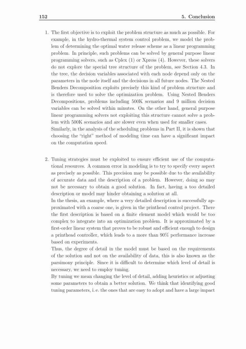
152 5. Conclusion
1. The first objective is to exploit the problem structure as much as possible. Forexample, in the hydro-thermal system control problem, we model the prob-lem of determining the optimal water release scheme as a linear programmingproblem. In principle, such problems can be solved by general purpose linearprogramming solvers, such as Cplex (1) or Xpress (4). However, these solversdo not explore the special tree structure of the problem, see Section 4.3. Inthe tree, the decision variables associated with each node depend only on theparameters in the node itself and the decisions in all future nodes. The NestedBenders Decomposition exploits precisely this kind of problem structure andis therefore used to solve the optimization problem. Using Nested BendersDecompositions, problems including 500K scenarios and 9 million decisionvariables can be solved within minutes. On the other hand, general purposelinear programming solvers not exploiting this structure cannot solve a prob-lem with 500K scenarios and are slower even when used for smaller cases.Similarly, in the analysis of the scheduling problems in Part II, it is shown thatchoosing the “right” method of modeling time can have a significant impacton the computation speed.
2. Tuning strategies must be exploited to ensure efficient use of the computa-tional resources. A common error in modeling is to try to specify every aspectas precisely as possible. This precision may be possible due to the availabilityof accurate data and the description of a problem. However, doing so maynot be necessary to obtain a good solution. In fact, having a too detaileddescription or model may hinder obtaining a solution at all.In the thesis, an example, where a very detailed description is successfully ap-proximated with a coarse one, is given in the printhead control project. Therethe first description is based on a finite element model which would be toocomplex to integrate into an optimization problem. It is approximated by afirst-order linear system that proves to be robust and efficient enough to designa printhead controller, which leads to a more than 90% performance increasebased on experiments.Thus, the degree of detail in the model must be based on the requirementsof the solution and not on the availability of data, this is also known as theparsimony principle. Since it is difficult to determine which level of detail isnecessary, we need to employ tuning.By tuning we mean changing the level of detail, adding heuristics or adjustingsome parameters to obtain a better solution. We think that identifying goodtuning parameters, i. e. the ones that are easy to adopt and have a large impact

5. Conclusion 153
on the solution quality, is very helpful in solving real world problems.Examples for tuning parameters are given in the hydro-thermal system con-trol problem. There it is shown that, for fixed computational resources, thesolution quality can be improved by changing the sampling frequency of therandom variable at different time stages in the prediction horizon of the con-troller.
3. The computations in the thesis show that models and problem formulationsneed to be tested using real world data.Researchers are often asked to provide general purpose solutions that can solvea large class of problems. However, the results in the thesis indicate that thisis only possible to a limited extent. When the application problems need tobe solved for realistic problem sizes, computational complexity often becomesa limitation. In such cases, no general purpose concept will help other than toprovide a problem specific controller design.For example, in Part II it is shown that neither discrete time nor contin-uous time formulations are in general superior for load tracking schedulingproblems. It is possible to model both, the workforce scheduling and the steelplant scheduling problem, as a discrete time and as continuous time schedulingproblem. However, the continuous time formulation of the workforce schedul-ing problem and the discrete time formulation of the steel scheduling problemare only able to solve unrealisticly small problem cases.Furthermore, we show that even if a formulation works well for a given prob-lem size, as specified by the number of variables and constraints, it may failto do so if the parameters in the problem are slightly changed.An example of this effect is shown in Part II. Here minimal variations in pa-rameter values, not the number of variables or constraints, lead to an increasein computation time by two orders of magnitude. Such results are difficult topredict. As a consequence a close collaboration between the control engineerand the industrial user is needed. The industrial user is likely to have the bestpossible estimates of what data can be expected and his expert knowledgeshould be included in the controller design process. Showing that a controller“works “ for an academic example might not be sufficient. Thus solutions of anapplication project should demonstrate that they can successfully solve testcases that were defined by the industrial user.

154 5. Conclusion
Summary
Altogether the applications in the three parts of the thesis demonstrate that so-phisticated controllers can be designed using techniques of optimal control. Wherenecessary these are augmented by stochastic variables, or the model of the timevariable is adopted to the special needs of the application. Also, various tuningpossibilities were shown for the different projects. As pointed out in the individualparts, these might be used to improve the performance of the controller or evento make a problem solvable at all. Yet, the projects also raise a number of openquestions that are discussed in the next chapter.

Bibliography 155
Bibliography
[1] Cplex (2006). ILOG CPLEX 10.0 User’s Maual. ILOG, France.
[2] Geyer, T., Papafotiou, G., & Morari, M. (2004). On the optimal control ofswitch-mode dc-dc converters. Hybrid Systems: Computation and Control, 2993,342–356.
[3] Löfberg, J. (2003). Minimax Approaches to Robust Model Predictive Control.Linköping studies in science and technology. thesis no 812, Linkoping University.
[4] Xpress (2007). Xpress-Optimizer Reference Manual Release 18.10. Dash Opti-mization.


6 Outlook
Application driven research lead to the solution of three industrial problems. How-ever, many ideas, concepts and findings apply to a broader range of problems. Asan outlook we propose to continue this road and extend the techniques for control ofswitched-input and uncertain systems. More precisely, for the applications discussedin this thesis, we list potential extensions and starting points for further research.
Printhead Control
For an industrial implementation of the printhead controller, a few problems stillremain that can further enhance the proposed controller.
• Investigation of the effects of neighboring heat elements:As discussed in Section 2.2, we neglect the effects of neighboring heat elementsin the current model. It is not clear, if this is a valid assumption and itshould be analyzed how large the effects from neighboring heat elements are.If necessary, an ad-hoc scheme to counteract these as e. g. proposed by Shigeru& Masanori (6) could be designed and tested.
• Controller switching during the ramp up and down phases of the print speed:The current controllers are designed for each print speed separately. However,during start and stop of the printer, it has to accelerate and decelerate untilthe final print speed is reached. For these ramp up and ramp down times asuitable scheme that switches among lookup tables for different speeds mustbe developed and tested.
• Inclusion of heat sink temperature variations in the controller:All current results were obtained for a “cold” printhead, i. e. one that has notbeen used heavily right before making a test printout. However, in indus-trial practice the printers are used for printing up to several hundred metersof printout at a time. In these situations the heat sink, that is mounted ontop of the printhead, and the interior of the printer heat up. This change inambient temperature of the heat elements affects their dynamics. Preliminary
157

158 6. Outlook
experimental results show that such changes should be considered by the con-troller. Since the temperature of the heat sink can be measured, we proposeto compute lookup tables for different heat sink temperatures. Based on themeasured heat sink temperature, the controller can chose the appropriate lookup table and thereby adapt to the changing temperature.
Load Tracking Scheduling
Analyzing load tracking scheduling problems is a first step in bringing together thefield of scheduling and the field of control engineering. Unlike traditional schedulingproblems, load tracking scheduling is concerned with the tracking of a referencesignal. This is the typical objective in control engineering problems. As an extensionof this research, we propose the following research directions:
• It should be examined what might be called a closed loop scheduling problem,where feedback is used to counteract disturbances. In the thesis, the focus is ontesting different formulations for load tracking scheduling problems. However,the analysis is done for a finite horizon open loop case only. In practice how-ever, load tracking problems may have long, possibly infinite, tracking signals.For such cases receding horizon policies should be investigated. In recedinghorizon policies, the schedule would be computed for a fixed horizon into thefuture and executed until a new solution is computed over a shifted horizon.Such a scheme might be able to solve scheduling problems for long horizons.Furthermore, the re-solving of the problem allows adjusting to unmodeledchanges that happen throughout the application.
• From a practical point of view, it would also be interesting to develop algo-rithms for robust scheduling. We define robust scheduling as a problem wherea schedule must be computed such that it remains feasible even if parameterschange within a pre-specified range. One of the difficulties in robust schedulingis that the resulting schedule should be robust for both changes in continuousparameters (such as variations in minimum or maximum processing durationsof tasks) as well as to changes in discrete parameters (such as availability ofa machine). In a research project, both of these parameter variations shouldbe investigated separately at first. This might be started by analysis of ex-isting schedules. The goal should be to first formulate an open loop controlproblem that computes a robust schedule for a given horizon into the future.Following the open loop control, it should be investigated if, and how, a robustscheduling might be extended to the closed loop case.

6. Outlook 159
Hydro-thermal System Control
In the hydro-thermal system control project we employed stochastic programmingtechniques in a closed loop control problem. To the best of our knowledge wepresented the first closed loop analysis of using multistage stochastic programmingfor MPC. However, the algorithms we used still have some deficiencies that shouldbe addressed in future research.
• A major drawback of using Monte-Carlo sampling to generate the event treefor the stochastic program is that it makes the computed control outputsstochastic, since for the same initial conditions the sampled event trees willdiffer almost surely. Thus, it is proposed to replace the Monte-Carlo samplingby a scheme that creates the event tree deterministically. One possible schemeis described by Pflug & Swietanowski (4), where an event tree is constructedin a deterministic way from the continuous distribution by minimization of theFortet-Mourier metric.
• Using Monte-Carlo sampling for the event tree generation does not guaranteefeasibility of the solution. As discussed in Section 4.4 the stochastic programdoes not guarantee feasibility since scenarios may occur that lie outside ofthose that are included in the event tree. The chances for scenarios leading toinfeasibility might be reduced by augmenting the tree with extreme scenariosas suggested by Dupacova (1). In a first step with this approach, feasibilityof the open loop problem might be guaranteed. In a second step, it might beexamined if, and how, feasibility for the closed loop case might be obtainedwhen using these results.
• The current setup uses Nested Benders Decomposition to solve the multistagestochastic program efficiently. Other decomposition schemes exist. Efficiencyof these should be investigated. In particular, it might be investigated whetherthe use of diagonal quadratic decomposition, see Ruszczynski & Shapiro (5),allows for larger event trees and leads to faster computation times. Also,it might be possible to use the decomposition scheme that was proposed byHaneveld & van der Vlerk (2) to solve the multistage stochastic program moreefficiently.Such an analysis is not only of interest from a stochastic programming pointof view, but also from a control engineering perspective, since the differentdecomposition schemes can also be used to solve min-max MPC problems asMunoz De La Pena et al. (3) demonstrated using Nested Benders Decomposi-tion.

Bibliography
[1] Dupacova, J. (1995). Stochastic programming: Approximation via scenarios. InProceedings of the 3rd International Conference on Approximation and Optimiza-
tion in the Caribbean.
[2] Haneveld, W. & van der Vlerk, M. (2006). Integrated chance constraints: Re-duced forms and an algorithm. Computational Management Science, 3(4), 245–269.
[3] Munoz De La Pena, D., Alamo, T., Bemporad, A., & Camacho, E. (2006). Adecomposition algorithm for feedback min-max model predictive control. IEEE
Transactions on Automatic Control, 51(10), 1688–1692.
[4] Pflug, G. & Swietanowski, A. (1998). Optimal scenario tree generation for mul-tiperiod financial optimization.
[5] Ruszczynski, A. & Shapiro, A. (2003). Stochastic Programming (Handbooks in
Operations Research and Management Series). Elsevier Publishing Company.
[6] Shigeru, A. & Masanori, S. (1987). Patent, 62227664 A, Thermal Printer Print
Control System (in Japanese). Alps Electric Co Ltd, Japanese Patent Office.


Curriculum Vitae
Kristian Nolde,
born on March 1, 1977 in Hamburg, Germany
2003-2008 PhD candidate at the Automatic Control Laboratory,ETH Zurich, Zurich Switzerland
2001-2003 Graduate studies in Systems Engineering at theTechnical University Hamburg-Harburg, HamburgGermany
2001 Graduate studies at the Graduate School of Arts andSciences, Harvard University, Cambridge, MA, USA
1997-2001 Undergraduate studies in General Engineering Sciencesat the Technical University Hamburg-Harburg,Hamburg Germany
1987-1996 Gymnasium Doerpsweg, Hamburg, Germany
1993-1994 Indian Springs School, Indian Springs, AL, USA