A Survey on Image-Based Rendering - Representation, Sampling and Compression

Cha Zhang and Tsuhan Chen Advanced Multimedia Processing Lab

1 2 L

1

2

M

u

v

t

s

Technical Report AMP 03-03 June 2003

Electrical and Computer Engineering Carnegie Mellon University

Pittsburgh, PA 15213

2

Abstract

Image-based rendering (IBR) has attracted a lot of research interest recently. In this paper, we

survey the various techniques developed for IBR, including representation, sampling and

compression. The goal is to provide an overview of research for IBR in a complete and

systematic manner. We observe that essentially all the IBR representations are derived from the

plenoptic function, which is seven dimensional and difficult to handle. We classify various IBR

representations into two categories based on how the plenoptic function is simplified, namely

restraining the viewing space and introducing source descriptions. In the former category, we

summarize six common assumptions that were often made in various approaches and discuss how

the dimension of the plenoptic function can be reduced based on these assumptions. In the latter

category, we further categorize the methods based on what kind of source description was

introduced, such as scene geometry, texture map or reflection model. Sampling and compression

are also discussed respectively for both categories.

I. Introduction

One might remember that in the movie Matrix, the scene with Keeanu Reeves dodging the bullets

might be one of the most spectacular images ever caught on camera. This filming technology is

what the movie producers called “Flo-Mo”. “Flo-Mo” lets the filmmakers shoot scenes where the

camera moves at a normal speed while the action is frozen or happens in slow motion. Two

movie cameras and 120 computer-controlled still cameras were used in that scene. Similarly, the

Eyevision system developed by CBS [11], which consisted of 33 cameras spaced approximately 6

degrees apart around the rim of the stadium, was used in a live broadcast of Super Bowl game in

Jan. 2001. It provided a unique 3D view of selected plays in a 270-degree stop action image.

These novel viewing experiences were brought to us by image-based rendering (IBR), which has

been a very active research topic recently. By capturing a set of images or light rays in the space,

the goal of IBR is to reproduce the scene correctly at an arbitrary viewpoint, with unknown or

limited amount of geometry. Compared with geometric models that dominate the traditional 3D

rendering pipelines, images are easier to obtain, simpler to handle and more realistic to render.

Moreover, since image processing is one of the most widely studied research topics in the

literature, IBR has attracted many researchers from different communities, including graphics,

vision and signal processing.

3

Since the goal of IBR is to capture and render the 3D world, let us first see how the world can

be described. One possible solution is to record all the objects in the world and their interactions,

which we call a source description. The traditional model-based rendering approach adopts such

a description: shapes of the objects are represented by certain geometric models; properties of the

object surfaces are described by texture maps and reflection models; lighting and shading are the

results of interaction between the light sources and objects, etc. The source description is often

compact and insightful, because it tells how the world is composed. However, it has the

disadvantage that such a description is not always available. From what we can observe with our

eyes or cameras, deriving the source description is not trivial, and has been the goal of computer

vision for more than twenty years with limited success.

( )zyx VVV ,,

( )ϕθ ,

λ,t

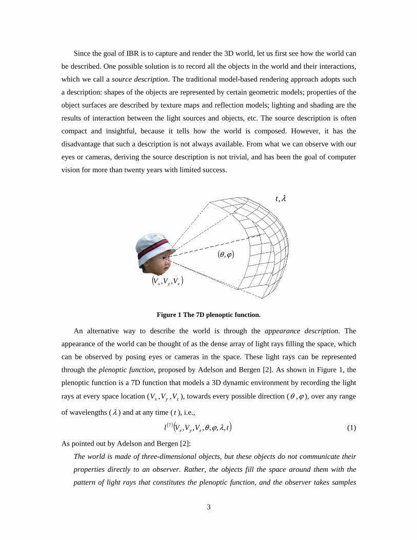
Figure 1 The 7D plenoptic function.

An alternative way to describe the world is through the appearance description. The

appearance of the world can be thought of as the dense array of light rays filling the space, which

can be observed by posing eyes or cameras in the space. These light rays can be represented

through the plenoptic function, proposed by Adelson and Bergen [2]. As shown in Figure 1, the

plenoptic function is a 7D function that models a 3D dynamic environment by recording the light

rays at every space location ( xV , yV , zV ), towards every possible direction (θ ,ϕ ), over any range

of wavelengths ( λ ) and at any time ( t ), i.e.,

( )( )tVVVl zyx ,,,,,,7 λϕθ (1)

As pointed out by Adelson and Bergen [2]:

The world is made of three-dimensional objects, but these objects do not communicate their

properties directly to an observer. Rather, the objects fill the space around them with the

pattern of light rays that constitutes the plenoptic function, and the observer takes samples

4

from this function. The plenoptic function serves as the sole communication link between the

physical objects and their corresponding retinal images. It is the intermediary between the

world and the eye.

When we take an image for a scene with a pinhole camera1, the light rays passing through the

camera’s center-of-projection are recorded. They can also be considered as samples of the

plenoptic function. As image-based rendering is based on images, it adopts the appearance

description. We define IBR under the plenoptic function framework as follows:

Definition - image based rendering: Given a continuous plenoptic function that describes a

scene, image-based rendering is a process of two stages – sampling and rendering2. In the

sampling stage, samples are taken from the plenoptic function for representation and storage. In

the rendering stage, the continuous plenoptic function is reconstructed with the captured samples.

The above definition reminds us about what we typically do in signal processing: given a

continuous signal, sample it and then reconstruct it. The uniqueness of IBR is that the plenoptic

function is 7D – a dimension beyond most of the signals handled before. In fact, the 7D function

is so general that, due to the tremendous amount of data required, no one has been able to sample

the full function into one representation. Research on IBR is mostly about how to make

reasonable assumptions to reduce the sample data size while keeping reasonable rendering

quality.

There have been many IBR representations invented in the literature. They basically follow

two major strategies in order to reduce the data size. First, one may restrain the viewing space of

the viewers. Such constraints will effectively reduce the dimension of the plenoptic function,

which makes sampling and rendering manageable. For example, if we limit the viewers’ interest

to static scenes, the time dimension in the plenoptic function can be simply dropped. Second, one

may introduce some source descriptions into IBR, such as the scene geometry. Source description

has the benefit that it can be very compact. A hybrid source-appearance description is definitely

attractive for reducing the data size. To obtain the source description, manual work may be

involved or we may resort to computer vision techniques.

1 Throughout this paper, we assume that the cameras we use are pinhole cameras. Most of the IBR

technologies in the literature made such assumption. The only exception, as far as the authors know, is the

work by Isaksen et al. [47], where the effects of various aperture and focus were studied. 2 We believe that considering IBR as a generic term for the techniques of both sampling and rendering is

more appropriate than the conventional definition in [82]. In the sections that follow, IBR rendering will be

used to refer to the rendering stage specifically.

5

Once the IBR representation of the scene has been determined, one may further reduce the

data size through sampling and compression. The sampling analysis can tell us what is the

minimum number of images / light rays that is necessary to render the scene at a satisfactory

quality. Compression, on the other hand, can further remove the redundancy inside and between

the captured images. Due to the high redundancy in many IBR representations, an efficient IBR

compression algorithm can easily reduce the data size by tens or hundreds of times.

In this paper, we survey the various techniques developed for IBR. Although other

classification methods are possible [48], we classify the techniques into two categories based on

the strategies they follow. Section II presents IBR approaches that restrain the viewing space.

Section III discusses about how to introduce source descriptions in order to reduce the data size.

Sampling and compression are discussed for different IBR representations in different sections.

Conclusions and future work are given in Section IV.

II. Restraining the Viewing Space

If the viewing space can be constrained, the amount of images required for reproducing the scene

can be largely reduced. Take an extreme example: if the viewer has to stay at one certain position

and view along one certain direction, an image or a video sequence captured at that position and

direction is good enough for representing the scene. Another example is branch movies

[68][108][85], in which segments of movies corresponding to different spatial navigation paths

are concatenated together at selected branch points, and the user is forced to move along the paths

but allowed to switch to a different path at the branch points.

A. Commonly Used Assumptions to Restrain the Viewing Space

There is a common set of assumptions that people made for restraining the viewing space in

IBR. Some of them are preferable, as they do not impact much on the viewers’ experiences. Some

others are more restrictive and used only when the storage size is a critical concern. We list them

below roughly based on their restrictiveness.

Assumption 1: As we are taking images of the scene for IBR, we may simplify the

wavelength dimension into three channels, i.e., the red, green and blue channels. Each channel

represents the integration of the plenoptic function over a certain wavelength range. This

simplification can be carried out throughout the capturing and rendering of IBR without

noticeable effects. Almost all the practical representations of IBR make this assumption.

Assumption 2: The air is transparent and the radiances along a light ray through empty space

remain constant. Under this assumption, we do not need to record the radiances of a light ray on

6

different positions along its path, as they are all the same. To see how we can make use of this

assumption, let us limit our interest to the light rays leaving the convex hull of a bounded scene

(if the viewer is constrained in a bounded free-space region, the discussion hereafter still applies).

Under Assumption 2, the plenoptic function can be represented by its values along an arbitrary

surface surrounding the scene. This reduces the dimension of the plenoptic function by one. The

radiance of any light ray in the space can always be obtained by tracing it back to the selected

surface. In other words, Assumption 2 allows us to capture a scene at some places and render it at

somewhere else. This assumption is also widely used, such as in [62][37][119]. However, a real

camera has finite resolution. A pixel in an image is in fact an average of the light rays from a

certain area on the scene surface. If we put two cameras on a line and capture the light ray along

it, they may have different results, as their observing area size on the scene surface may be very

different. Such resolution sensitivity was pointed out by Buehler et al. in [10].

Assumption 3: The scene is static, thus the time dimension can be dropped. Although a

dynamic scene includes much more information than a static one, there are practical concerns that

restrict the popularity of dynamic IBR. One concern is the sample data size. We all know that if

we capture a video for a scene instead of a single image, the amount of data may increase for

about 2 or 3 orders of magnitude. It can be expected that dynamic IBR will have the same order

of size increase from static IBR. Moreover, IBR often requires a large amount of capturing

cameras. If we want to record a dynamic scene, all these cameras must be present and capturing

video together. Unfortunately, today’s practical systems cannot afford to have that many cameras.

The known IBR camera array that has the largest number of cameras may be the Stanford light

field video camera [137], which consists of 128 cameras. This is yet not enough for rendering

high quality images. Capturing static scenes does not have the above problem, because we can

always use the time axis to compensate for the lack of cameras. That is, images captured at

different time and positions can be used together to render novel views.

Assumption 4: In stead o moving in the 3D space, the viewer is constrained to be on a

surface, e.g., the ground plane. The plenoptic function can then reduce one dimension, as the

viewer’s space location becomes 2D. Although restricting the viewer on a surface seems

unpleasing, Assumption 4 is acceptable for two reasons. First, the eyes of human beings are

usually at a certain height-level for walk-through applications. Second, human beings are less

sensitive to vertical parallax and lighting changes because their two eyes are spaced horizontally.

Example scenes using concentric mosaics [119] showed that strong effects of 3D motion and

lighting change could still be achieved under this assumption.

7

Assumption 5: The viewer moves along a certain path. That is, the viewer can move forward

or backward along that path, but he / she cannot move off the path. Assumption 5 reduces two

dimensions from the full plenoptic function. Branch movies [68][108][85] is an example that

takes this assumption. This assumption is also reasonable for applications such as virtual touring,

where the viewer follows a predefined path to view a large scene [52][89].

Assumption 6: The viewer has a fixed position. This is the most restrictive assumption,

which reduces the dimension of the plenoptic function by three. No 3D effects can possibly be

perceived under this assumption. Nevertheless, under this assumption the representations of IBR

can be very compact and bear much similarity to regular images and videos. Capturing such

representations is also straightforward. Thanks to these benefits, the QuickTime VRTM technology

[20] based on Assumption 6 has become the most popular one among all the IBR approaches in

practice.

There is one important thing to notice. That is, the dimension reduced by the above six

assumptions may not be addable. In particular, Assumption 2 does not help further save

dimension so long as one of the Assumption 4, 5 or 6 is made. This is because when the viewer’s

position has certain constraints, usually the sampled light ray space intersects each light ray only

at a single point, which makes Assumption 2 not useful any more. In the next subsection, we will

show a concrete example with concentric mosaics [119].

B. Various Representations and Their Rendering Process

By making the assumptions mentioned above, the 7D plenoptic function can be simplified to

lower dimensional functions, from 6D to 2D. A quick summary of some popular representations

is given in Table 1. We will explain these techniques in detail.

6D – The surface plenoptic function

The surface plenoptic function (SPF) was first introduced in [149]. It is simplified from the full

7D plenoptic function using Assumption 2. As we discussed, when radiance along a light ray

through empty space remains constant, the plenoptic function can be represented by its values on

any surface surrounding the scene. SPF chooses the surface as the scene surface itself. For regular

scene surface with dimension 2, the SPF is 6D: position on the surface (2D), light ray direction

(2D), time (1D) and wavelength (1D). Although it is difficult to apply SPF for capturing real

scenes due to unknown scene geometry, SPF was used in [149] for analyzing the Fourier

spectrum of IBR representations (see more details in Section II-C). The surface light field

[86][139] could be considered as dimension-reduced version of SPF.

8

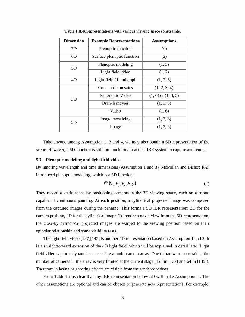
Table 1 IBR representations with various viewing space constraints.

Dimension Example Representations Assumptions

7D Plenoptic function No

6D Surface plenoptic function (2)

Plenoptic modeling (1, 3) 5D

Light field video (1, 2)

4D Light field / Lumigraph (1, 2, 3)

Concentric mosaics (1, 2, 3, 4)

Panoramic Video (1, 6) or (1, 3, 5)

Branch movies (1, 3, 5) 3D

Video (1, 6)

Image mosaicing (1, 3, 6) 2D

Image (1, 3, 6)

Take anyone among Assumption 1, 3 and 4, we may also obtain a 6D representation of the

scene. However, a 6D function is still too much for a practical IBR system to capture and render.

5D – Plenoptic modeling and light field video

By ignoring wavelength and time dimensions (Assumption 1 and 3), McMillan and Bishop [82]

introduced plenoptic modeling, which is a 5D function:

( )( )ϕθ ,,,,5zyx VVVl (2)

They record a static scene by positioning cameras in the 3D viewing space, each on a tripod

capable of continuous panning. At each position, a cylindrical projected image was composed

from the captured images during the panning. This forms a 5D IBR representation: 3D for the

camera position, 2D for the cylindrical image. To render a novel view from the 5D representation,

the close-by cylindrical projected images are warped to the viewing position based on their

epipolar relationship and some visibility tests.

The light field video [137][145] is another 5D representation based on Assumption 1 and 2. It

is a straightforward extension of the 4D light field, which will be explained in detail later. Light

field video captures dynamic scenes using a multi-camera array. Due to hardware constraints, the

number of cameras in the array is very limited at the current stage (128 in [137] and 64 in [145]).

Therefore, aliasing or ghosting effects are visible from the rendered videos.

From Table 1 it is clear that any IBR representation below 5D will make Assumption 1. The

other assumptions are optional and can be chosen to generate new representations. For example,

9

if we constrain the viewer to be on a surface (Assumption 4), we get another 5D representation.

Although no work has been reported to take such a representation, it is obviously feasible. What

we need to do is to put many cameras on the viewer’s surface and capture video sequences.

During the rendering, since we did not make Assumption 2, the rendering position is also

restricted on that surface.

4D – Light field / Lumigraph

The most well-known 4D IBR representations are the light field [62] and the Lumigraph [37].

They both ignored the wavelength and time dimensions and assumed that radiance does not

change along a line in free space (Assumption 1, 2 and 3). However, parameterizing the space of

oriented lines is still a tricky problem. The solutions they came out happened to be the same: light

rays are recorded by their intersections with two planes. One of the planes is indexed with

coordinate ( )vu, and the other with coordinate ( )ts, , i.e.:

( )( )vutsl ,,,4 (3)

v

us

t

(u0,v0)

(s0,t0)

Light ray

z

Object

Focal planeCamera plane

Discretized point

Novel viewposition

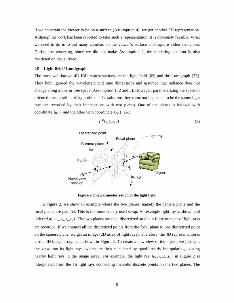
Figure 2 One parameterization of the light field.

In Figure 2, we show an example where the two planes, namely the camera plane and the

focal plane, are parallel. This is the most widely used setup. An example light ray is shown and

indexed as ( )0000 ,,, tsvu . The two planes are then discretized so that a finite number of light rays

are recorded. If we connect all the discretized points from the focal plane to one discretized point

on the camera plane, we get an image (2D array of light rays). Therefore, the 4D representation is

also a 2D image array, as is shown in Figure 3. To create a new view of the object, we just split

the view into its light rays, which are then calculated by quad-linearly interpolating existing

nearby light rays in the image array. For example, the light ray ( )0000 ,,, tsvu in Figure 2 is

interpolated from the 16 light rays connecting the solid discrete points on the two planes. The

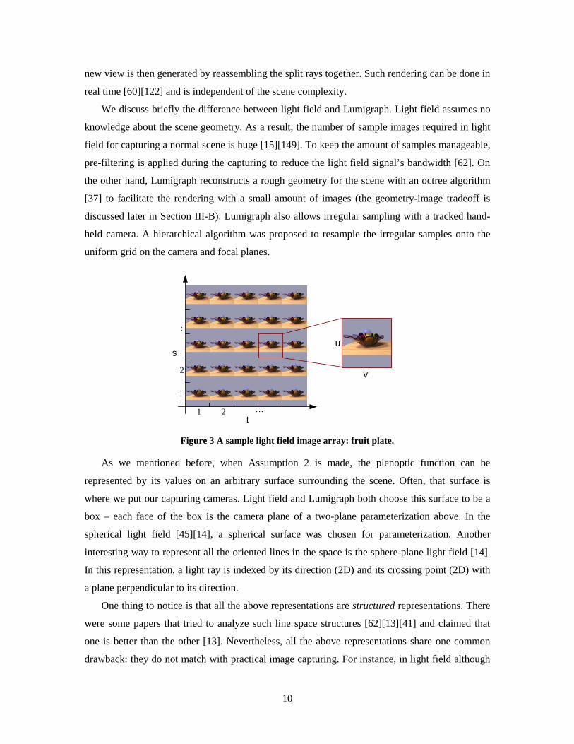
10

new view is then generated by reassembling the split rays together. Such rendering can be done in

real time [60][122] and is independent of the scene complexity.

We discuss briefly the difference between light field and Lumigraph. Light field assumes no

knowledge about the scene geometry. As a result, the number of sample images required in light

field for capturing a normal scene is huge [15][149]. To keep the amount of samples manageable,

pre-filtering is applied during the capturing to reduce the light field signal’s bandwidth [62]. On

the other hand, Lumigraph reconstructs a rough geometry for the scene with an octree algorithm

[37] to facilitate the rendering with a small amount of images (the geometry-image tradeoff is

discussed later in Section III-B). Lumigraph also allows irregular sampling with a tracked hand-

held camera. A hierarchical algorithm was proposed to resample the irregular samples onto the

uniform grid on the camera and focal planes.

1 2 L

1

2

M

u

v

t

s

Figure 3 A sample light field image array: fruit plate.

As we mentioned before, when Assumption 2 is made, the plenoptic function can be

represented by its values on an arbitrary surface surrounding the scene. Often, that surface is

where we put our capturing cameras. Light field and Lumigraph both choose this surface to be a

box – each face of the box is the camera plane of a two-plane parameterization above. In the

spherical light field [45][14], a spherical surface was chosen for parameterization. Another

interesting way to represent all the oriented lines in the space is the sphere-plane light field [14].

In this representation, a light ray is indexed by its direction (2D) and its crossing point (2D) with

a plane perpendicular to its direction.

One thing to notice is that all the above representations are structured representations. There

were some papers that tried to analyze such line space structures [62][13][41] and claimed that

one is better than the other [13]. Nevertheless, all the above representations share one common

drawback: they do not match with practical image capturing. For instance, in light field although

11

we may place cameras on the camera plane at the exact positions where discrete samples were

taken, the pixel coordinates of the captured images cannot coincide with the focal plane samples.

A sheared perspective projection was taken to compensate this [62]. In Lumigraph the images

were taken with a hand-held camera so a resampling process was required any way. Spherical

light field requires all the sample light rays passing through the corners of the subdivided sphere

surface, which demands resampling for practical capturing. The sphere-plane light field does not

have pencil (a set of rays passing through the same point in space [2]) in the representation so

resampling is also needed. It would be attractive to store and render scenes from the captured

images directly. In Section III-A we will discuss unstructured Lumigraph [10], which does not

require the resampling.

Similar to the discussions in 5D, there are other possibilities to generate 4D IBR

representations. For example, by making Assumption 1, 3 and 4, we may capture a static scene

for a viewer to move smoothly on a surface [5][20]. If we make Assumption 1 and 5, we may

record a dynamic event and allow a viewer to move back and forth along a predefined path.

3D – Concentric mosaics and panoramic video

Other than the assumptions made in light field (Assumption 1, 2 and 3), concentric mosaics [119]

further restricts that both the cameras and the viewers are on a plane (Assumption 4), which

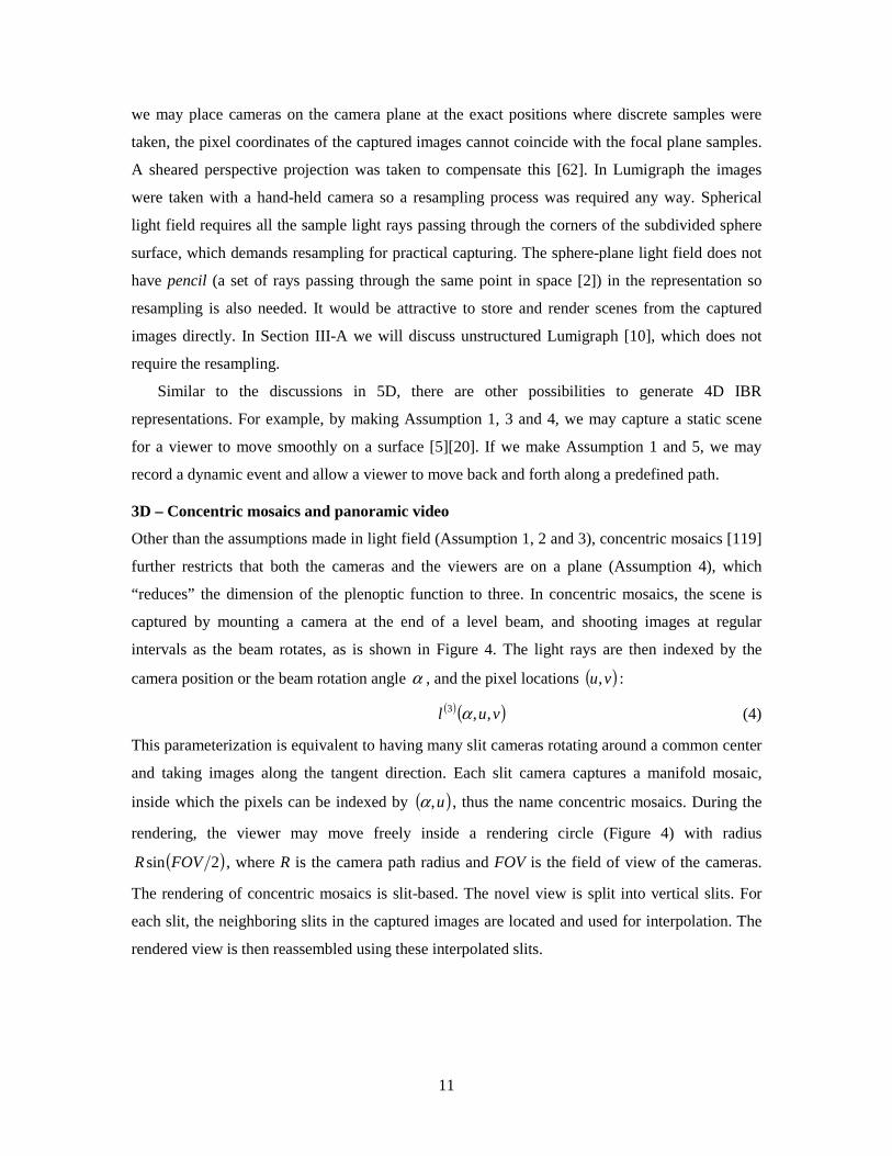
“reduces” the dimension of the plenoptic function to three. In concentric mosaics, the scene is

captured by mounting a camera at the end of a level beam, and shooting images at regular

intervals as the beam rotates, as is shown in Figure 4. The light rays are then indexed by the

camera position or the beam rotation angle α , and the pixel locations ( )vu, :

( )( )vul ,,3 α (4)

This parameterization is equivalent to having many slit cameras rotating around a common center

and taking images along the tangent direction. Each slit camera captures a manifold mosaic,

inside which the pixels can be indexed by ( )u,α , thus the name concentric mosaics. During the

rendering, the viewer may move freely inside a rendering circle (Figure 4) with radius

( )2sin FOVR , where R is the camera path radius and FOV is the field of view of the cameras.

The rendering of concentric mosaics is slit-based. The novel view is split into vertical slits. For

each slit, the neighboring slits in the captured images are located and used for interpolation. The

rendered view is then reassembled using these interpolated slits.

12

R

Camera path

Camera

Beam

Rotate

v

u

α

Rendering circle

FOV

Figure 4 Concentric mosaic capturing.

There is a severe problem with concentric mosaics – the vertical distortion. Unfortunately, no

matter how dense we capture the scene on the camera path, vertical distortion cannot be

eliminated. In the original concentric mosaics paper [119], depth correction was used to reduce

the distortion. That is, we need to have some rough knowledge about the scene geometry.

Ignoring how difficult it is to obtain the geometry information, recall in the last subsection that

the dimension reduced by Assumption 2 and Assumption 4 are not addable, we realize that the

light ray space concentric mosaics is capturing is in fact still 4D. Recording it with 3D data must

require extra information for rendering, in this case, the scene geometry.

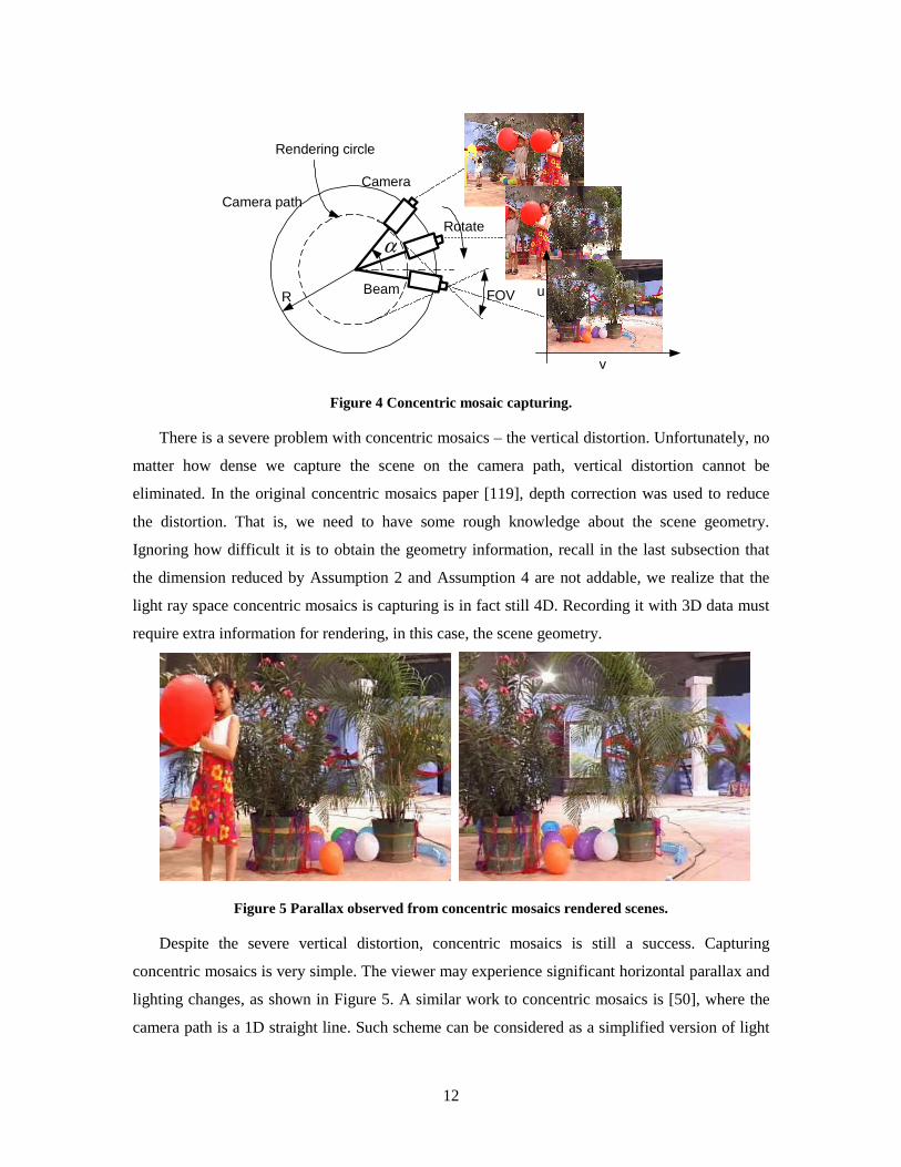
Figure 5 Parallax observed from concentric mosaics rendered scenes.

Despite the severe vertical distortion, concentric mosaics is still a success. Capturing

concentric mosaics is very simple. The viewer may experience significant horizontal parallax and

lighting changes, as shown in Figure 5. A similar work to concentric mosaics is [50], where the

camera path is a 1D straight line. Such scheme can be considered as a simplified version of light

13

field. On the other hand, concentric mosaics can be easily boosted to 4D if we align a vertical

array of cameras at the end of the beam [65].

Another popular 3D IBR representation is the panoramic video [20][35][89]. It can be used

for either dynamic (fixed viewpoint, Assumption 1 and 6) or static scenes (Assumption 1, 3 and

5). Compared with regular video sequences, the field of view in panoramic video is often 360º,

which allows the viewer to pan and zoom interactively. If the scene is static, the viewer can also

move around [20][52]. Capturing a panoramic video is an easy task. We simply capture a video

sequence by a multi-camera system [35][123], or an omnidirectional camera [88], or a camera

with fisheye lens [144]. Rendering of panoramic video only involves a warping from cylindrical

or spherical projected images to planar projected images. Due to the convenience of capturing

and rendering, the acceptable perceptual quality and the affordable storage requirement, multi-

panorama representations are adopted for several systems used to capturing large-scale scenes,

such as in [51][129]. Many commercial panoramic video systems are also available, such as iPIX

immersive imaging from Internet Pictures Corp.[46], 360 One VRTM from Kaidan [1],

TotalViewTM from Be Here Technologies [132], LadybugTM from Point Grey [54], among many

others.

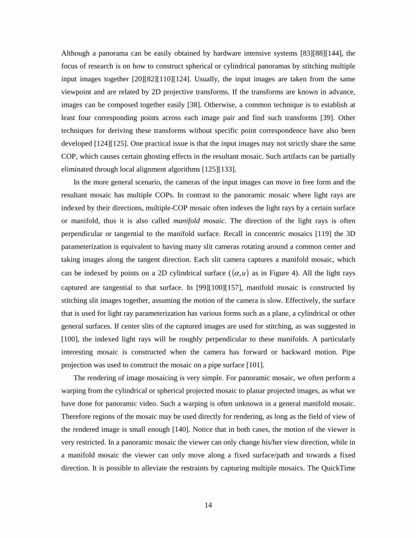
2D – Image mosaicing

Image mosaicing composes one single mosaic with multiple input images. The output mosaic is a

2D plenoptic function. Often such mosaic is composed for increasing the field of view of the

camera, with early applications in aerial photography [42][84] and cel animation [140].

Depending on the collection of the light rays recorded in the mosaic, image mosaicing techniques

can be classified into two categories: single-center-of-projection mosaic or multiple-center-of-

projection mosaic.

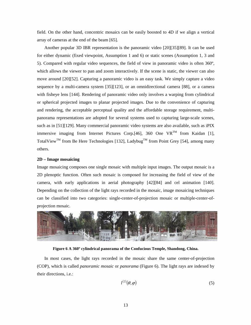
Figure 6 A 360º cylindrical panorama of the Confucious Temple, Shandong, China.

In most cases, the light rays recorded in the mosaic share the same center-of-projection

(COP), which is called panoramic mosaic or panorama (Figure 6). The light rays are indexed by

their directions, i.e.:

( )( )ϕθ ,2l (5)

14

Although a panorama can be easily obtained by hardware intensive systems [83][88][144], the

focus of research is on how to construct spherical or cylindrical panoramas by stitching multiple

input images together [20][82][110][124]. Usually, the input images are taken from the same

viewpoint and are related by 2D projective transforms. If the transforms are known in advance,

images can be composed together easily [38]. Otherwise, a common technique is to establish at

least four corresponding points across each image pair and find such transforms [39]. Other

techniques for deriving these transforms without specific point correspondence have also been

developed [124][125]. One practical issue is that the input images may not strictly share the same

COP, which causes certain ghosting effects in the resultant mosaic. Such artifacts can be partially

eliminated through local alignment algorithms [125][133].

In the more general scenario, the cameras of the input images can move in free form and the

resultant mosaic has multiple COPs. In contrast to the panoramic mosaic where light rays are

indexed by their directions, multiple-COP mosaic often indexes the light rays by a certain surface

or manifold, thus it is also called manifold mosaic. The direction of the light rays is often

perpendicular or tangential to the manifold surface. Recall in concentric mosaics [119] the 3D

parameterization is equivalent to having many slit cameras rotating around a common center and

taking images along the tangent direction. Each slit camera captures a manifold mosaic, which

can be indexed by points on a 2D cylindrical surface ( ( )u,α as in Figure 4). All the light rays

captured are tangential to that surface. In [99][100][157], manifold mosaic is constructed by

stitching slit images together, assuming the motion of the camera is slow. Effectively, the surface

that is used for light ray parameterization has various forms such as a plane, a cylindrical or other

general surfaces. If center slits of the captured images are used for stitching, as was suggested in

[100], the indexed light rays will be roughly perpendicular to these manifolds. A particularly

interesting mosaic is constructed when the camera has forward or backward motion. Pipe

projection was used to construct the mosaic on a pipe surface [101].

The rendering of image mosaicing is very simple. For panoramic mosaic, we often perform a

warping from the cylindrical or spherical projected mosaic to planar projected images, as what we

have done for panoramic video. Such a warping is often unknown in a general manifold mosaic.

Therefore regions of the mosaic may be used directly for rendering, as long as the field of view of

the rendered image is small enough [140]. Notice that in both cases, the motion of the viewer is

very restricted. In a panoramic mosaic the viewer can only change his/her view direction, while in

a manifold mosaic the viewer can only move along a fixed surface/path and towards a fixed

direction. It is possible to alleviate the restraints by capturing multiple mosaics. The QuickTime

15

hopping [20] and the manifold hopping [121] are two such extensions for panoramic mosaic and

manifold mosaic, respectively.

Other than increasing the field of view of the camera, image mosaicing can also be used to

increase the image resolution, namely super-resolution. We refer the reader to [9] for a review of

this area.

C. Sampling

In the last subsection, we discussed the various representations IBR may take and their rendering

schemes, given that different viewing space constraints are employed. This answers the question

how to sample and reconstruct the plenoptic function. However, there is one more question to

ask: how many samples do we need for anti-aliasing reconstruction? We refer this problem as the

IBR sampling problem and discuss its answers in this subsection.

IBR sampling is a very difficult problem, as the plenoptic function is such a high dimensional

signal. Obviously, the sampling rate will be determined by the scene geometry, the texture on the

scene surface, the reflection property of the scene surface, the motion of the scene objects, the

specific IBR representation we take, the capturing and the rendering camera’s resolution, etc.

Over-sampling was widely adopted in the early stages, as no solution to the sampling problem

was available. To reduce the huge amount of data recorded due to over-sampling, people used to

resort to various compression schemes to save the storage space, which will be described in

Subsection D. This situation was improved in the year 2000, when several pioneering papers were

published on IBR sampling [66][15][17].

As was pointed out in [17], IBR sampling is essentially a multi-dimensional signal processing

problem. Following the classic sampling theorem [96][31], one may first find the Fourier

transform of the plenoptic function and then sample it according to its spectrum bandwidth.

Nevertheless, although performing the Fourier transform of the 7D plenoptic function is possible

in theory, in practice we have to reduce the dimension of the signal. Again we check the

assumptions discussed in Subsection A and see how they may affect our sampling analysis.

Based on Assumption 1, the wavelength dimension can be ignored in most IBR applications.

Thus sampling along the wavelength axis can also be ignored. Assumption 2 claims that the

radiance of a light ray along its path remains constant in empty space. This means that along the

light ray path, one sample is good enough for perfect reconstruction. In reality, although the

resolution of real cameras is finite and Assumption 2 may not be strictly valid [10], the sampling

along the light ray path is still less interesting because the variation of the radiance is often too

slow. Assumption 3 said that if necessary, the time dimension could also be ignored. In practice,

16

even if we are capturing a dynamic scene, sampling on the time axis is often determined by the

camera’s frame rate and the property of the human eyes’ temporal perception [23]. Due to the

above reasons, most IBR sampling work in the literature [66][15][77][149] was for the light field

and concentric mosaics.

The earliest IBR sampling work was by Lin and Shum [66]. They performed sampling

analysis on both lightfield and concentric mosaics with the scale-space theory. The world is

modeled by a single point sitting at a certain distance to the cameras. Assuming using constant

depth and bilinear interpolation during the rendering, the bounds are derived from the aspect of

geometry and based on the goal that no “spurious detail” should be generated during the

rendering (referred as the causality requirement). Although the viewpoint of their analysis is

rather interesting, this method is constrained by the simple world model they chose. The texture

and the reflection model of the scene surface and occlusions are hard to analyze with such a

method.

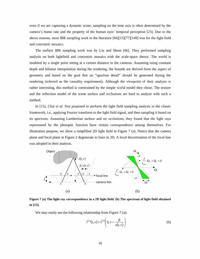
In [15], Chai et al. first proposed to perform the light field sampling analysis in the classic

framework, i.e., applying Fourier transform to the light field signal, and then sampling it based on

its spectrum. Assuming Lambertian surface and no occlusions, they found that the light rays

represented by the plenoptic function have certain correspondence among themselves. For

illustration purpose, we show a simplified 2D light field in Figure 7 (a). Notice that the camera

plane and focal plane in Figure 2 degenerate to lines in 2D. A local discretization of the focal line

was adopted in their analysis.

ft

v0 'v

( )vtz ,

( )vtzft ,

0

0 vfocal line

camera line

Object

tΩ

vΩπ

π−

0max

=Ω+Ω tvz

f

0min

=Ω+Ω tvz

f

B∆

(a) (b)

Figure 7 (a) The light ray correspondence in a 2D light field. (b) The spectrum of light field obtained

in [15].

We may easily see the following relationship from Figure 7 (a):

( )( ) ( )( )

−=

vtz

ftvlvtl

,,0, 22 (6)

17

where ( )vtz , is the scene depth of the light ray ( )vt, . When the scene is at constant depth

( ) 0, zvtz = , its Fourier transform can be written as:

( )( ) ( )

Ω+ΩΩ=ΩΩ tvvvt z

fLL

0

2 ', δ (7)

where ( )vL Ω' is the Fourier transform of ( )( )vl ,02 and ( )⋅δ is the 1D Dirac delta function.

Obviously the spectrum has non-zero values only along a line. When the scene depth is varying

between a certain range, a “truncating windows” analysis was given in the paper, which

concludes that the spectral support of a lightfield signal is bounded by the minimum and

maximum depths of objects in the scene only, no matter how complicated the scene is (Figure 7

(b)). Such analysis provides a fairly good first-order approximation of the spectrum analysis of

IBR. However, the dependency on mapping images captured at arbitrary position to that at the

origin prevents it from being applied to more complicated scenes such as non-Lambertian surface,

scenes with occlusions and other IBR methods such as concentric mosaics.

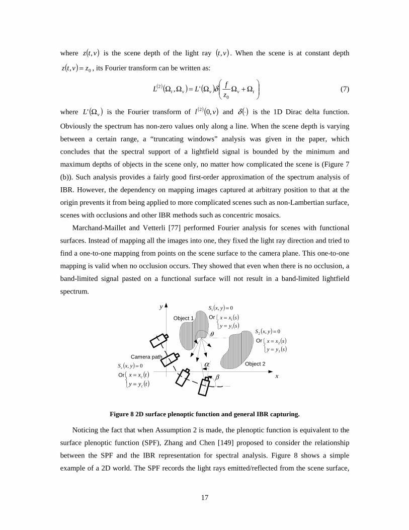
Marchand-Maillet and Vetterli [77] performed Fourier analysis for scenes with functional

surfaces. Instead of mapping all the images into one, they fixed the light ray direction and tried to

find a one-to-one mapping from points on the scene surface to the camera plane. This one-to-one

mapping is valid when no occlusion occurs. They showed that even when there is no occlusion, a

band-limited signal pasted on a functional surface will not result in a band-limited lightfield

spectrum.

( ) 0,1 =yxS

x

y

θ

Or ( )( )

==

syy

sxx

1

1

( ) 0,2 =yxS

Or ( )( )

==

syy

sxx

2

2

Object 1

Object 2Camera path

αβ

( ) 0, =yxSc

Or ( )( )

==

tyy

txx

c

c

Figure 8 2D surface plenoptic function and general IBR capturing.

Noticing the fact that when Assumption 2 is made, the plenoptic function is equivalent to the

surface plenoptic function (SPF), Zhang and Chen [149] proposed to consider the relationship

between the SPF and the IBR representation for spectral analysis. Figure 8 shows a simple

example of a 2D world. The SPF records the light rays emitted/reflected from the scene surface,

18

represented as ( )( )θ,2 sli , where s is the arc length on the scene surface curve; θ is the direction; i

is the index of objects. The IBR representation can be written as ( )( )α,2 tlc , where t is the arc

length on the camera path, α is the light ray direction. There exists an onto mapping from

( )( )θ,2 sli to ( )( )α,2 tlc due to the light ray correspondence. By assuming certain spectrum property

of the SPF, the paper showed that it is possible to obtain the spectrum of the IBR representation,

even when the scene is non-Lambertian or occluded. Moreover, the same methodology is

applicable for concentric mosaics. “Truncating windows” analysis can also be used when the

scene geometry is not available.

Same as in [77], analysis in [149] also showed that the spectrum of the IBR representation is

very easy to be band-unlimited. However, from an engineering point of view, most of the signal’s

energy is still located in a bounded region. We may sample the signal rectangularly [15] or non-

rectangularly [148] based on the high-dimensional generalized sampling theory [31].

Surprisingly, the non-rectangular sampling approach [148] does not show much improvement

over the rectangular one considering the gain in rendering quality and the extra complexity

introduced during the capturing and rendering.

It is also possible to sample the images non-uniformly for IBR [112][150][151]. Since most

of these approaches were discussed assuming certain knowledge about the scene geometry, we

discuss them in Section III-C.

D. Compression

Although we may reduce the number of images we take for IBR to the minimum through the

sampling analysis, the amount of images needed is still huge. For instance, the example scenes in

[15] shows that with constant depth rendering, the number of required images is on the order of

thousands or tens of thousands for light field. To further reduce the storage requirement for IBR,

data compression is the solution.

IBR compression bears much similarity as image or video compression, because IBR is often

captured as a sequence of images. In fact, most of the IBR techniques developed so far are

originated from image or video compression. On the other hand, IBR compression has its own

characteristics. As pointed out in [64], images in IBR have better cross-frame correlations

because of the regular camera motions. Thus we should expect better compression performance

for IBR. The reaction of the human visual system (HVS) to the distortions introduced in IBR

compression is also worth studying at very high compression ratio. Most importantly, since

during the IBR rendering any captured light ray may be used for interpolation, it is desirable that

19

the compressed bitstream is random-accessible so that we do not need to decompress all the light

rays into memory. Such property is also important for online streaming of IBR data.

Vector quantization (VQ) is often the first resort for data reduction in IBR [62][119]. As a

universal method, vector quantization provides reasonable compression ratio (around 10:1 to 20:1

as reported) and fast decoding speed. The code index of VQ is fixed-length, which is random-

accessible and has potential applications in robust online streaming. On the other hand, VQ does

not fully make use of the high correlations inside and between the captured images, thus the

compression ratio is not satisfactory.

The various image compression algorithms can also be applied to individual IBR images

without change. Miller et al. used the standard DCT-based JPEG algorithms for light field

compression [86] and obtained a compression ratio higher than that of VQ (around 20:1). The

more recent wavelet-based JPEG2000 standard [127] may further improve the performance, as

well as add features such as scalability. Since variable length coding (VLC) is employed, the light

ray access speed is not as fast as VQ. Yet it is still good enough for real-time rendering. The

limitation is that the inter frame correlation is not utilized, thus the compression ratio is still

relatively low.

Most of the IBR compression methods proposed so far [75][153][61][72][71] resemble video

coding, with certain modifications to the specific characteristics of IBR data. To see the close

relationship between them, we list the techniques in video coding and IBR compression in

parallel in Table 2. Detailed explanation follows.

The basic video coding techniques include motion compensation (MC), discrete cosine

transform (DCT), quantization and VLC, among many others. The images are divided into two

categories: intra frames and inter frames. Intra frames are often distributed uniformly and

encoded independently, while inter frames are predicted from neighboring intra frames through

MC. The early and widely adopted video coding standard, MPEG-2 [87], is a good example for

all these techniques. An intuitive approach for IBR compression is to apply these methods

directly for the IBR image sequence. In [120], Shum et al. proposed to compress the concentric

mosaics with MPEG-2. Both the captured images and the rebinned manifold mosaics were used

as frames in MPEG-2. The compression ratio was about 50:1. To facilitate random access,

pointers to the start positions of each vertical group of macroblocks (MB) were built into the

bitstream. Direct extension of the above approach for panoramic video and simplified dynamic

light field (videos taken at regularly spaced locations along a line) were given in [91] and [16],

respectively.

20

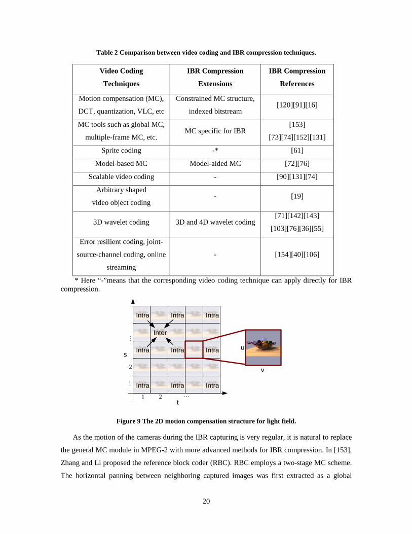
Table 2 Comparison between video coding and IBR compression techniques.

Video Coding

Techniques

IBR Compression

Extensions

IBR Compression

References

Motion compensation (MC),

DCT, quantization, VLC, etc

Constrained MC structure,

indexed bitstream [120][91][16]

MC tools such as global MC,

multiple-frame MC, etc. MC specific for IBR

[153]

[73][74][152][131]

Sprite coding -* [61]

Model-based MC Model-aided MC [72][76]

Scalable video coding - [90][131][74]

Arbitrary shaped

video object coding - [19]

3D wavelet coding 3D and 4D wavelet coding [71][142][143]

[103][76][36][55]

Error resilient coding, joint-

source-channel coding, online

streaming

- [154][40][106]

* Here “-”means that the corresponding video coding technique can apply directly for IBR compression.

1 2 L

1

2

M

t

su

v

Intra Intra

Inter

Intra

Intra IntraIntra

Intra IntraIntra

Figure 9 The 2D motion compensation structure for light field.

As the motion of the cameras during the IBR capturing is very regular, it is natural to replace

the general MC module in MPEG-2 with more advanced methods for IBR compression. In [153],

Zhang and Li proposed the reference block coder (RBC). RBC employs a two-stage MC scheme.

The horizontal panning between neighboring captured images was first extracted as a global

21

horizontal translation motion vector. Local MC refinement was used to further reduce the MC

residue. Another strength of RBC was the extensive usage of caches during the rendering, which

guaranteed the so-called just-in-time rendering. In the light field, cameras are arranged on a 2D

plane. Thus the MC structure should also be 2D. As shown in Figure 9, intra frames are uniformly

distributed on the 2D plane. Given any inter frame, four neighboring intra frames are often

available and can all be use for MC [73][75][152]. Hierarchical MC was proposed in

[131][74][75], where images are grouped into different levels through down-sampling on the

camera plane. The images at the lowest level are intra-coded. Higher level images are predicted

from lower level images. Such hierarchical MC structure improves the compression ratio, but its

bitstream may not be random accessible.

Further development on motion compensation includes sprite based coding and model based

coding. In [61], Leung and Chen proposed a sprite based compression method for concentric

mosaics. A sprite is generated by sticking the central slits of all the captured images. In fact, the

result is roughly a cylindrical panorama. The sprite is intra coded and all the captured images are

coded based on predictions from the sprite. Such a scheme has good random accessibility, and its

compression ratio is comparable to that of [153]. When the scene geometry is available

[32][107][114], it can greatly enhance the image prediction [72][76]. A hierarchical prediction

structure is still adopted [72], where the intra coded images and the geometry model are used

jointly to predict inter frames. In [76], images are mapped back onto the geometry model as view

dependent texture maps. These texture maps are then encoded through a 4D wavelet codec.

Model based IBR compression methods often report very high compression ratio, though such

performance heavily relies on how good the geometry model is.

Two key components in the recent MPEG-4 video coding standard are the scalable video

coding and arbitrary shaped video object coding [102]. Scalable video coding includes spatial

scalability, temporal scalability, SNR fine granularity scalability (FGS), and object-based

scalability. Ng et al. proposed a spatial scalability approach for the compression of concentric

mosaics in [90]. By using a nonlinear perfect reconstruction filter bank, images are decomposed

into different frequency bands and encoded separately with the MPEG-2 standard method.

Consider the scenario of online streaming. A low-resolution image may be rendered first when

the compressed base band bitstream arrives and refined later when more data are received.

Temporal scalability is applicable to dynamic scene IBR representations such as light field video

or panoramic video. Or, it can be considered as the scalability across different captured images.

The above-mentioned hierarchical MC based IBR compression algorithms [131][74][75] are good

examples. SNR FGS scalability and object-based scalability have not been employed in IBR

22

compression yet, but such methods should not be difficult to develop. Arbitrary shaped video

object coding may improve the compression performance because it improves the motion

compensation, removes the background, and avoids coding the discontinuity around the object

boundary. It was adopted in a recent paper for light field compression [19].

3D wavelet coding presents another category of methods for video coding [128][93][130]. In

[71], Luo et al. applied 3D wavelet coding for concentric mosaics. Nevertheless, its compression

ratio is not satisfactory due the poor cross-frame filtering performance, which is consistent with

the results reported in 3D wavelet video coding. A smart-rebinning approach was proposed in

[143] which reorganized the concentric mosaics data into a set of panoramas. Such rebinning

process greatly enhanced the cross-frame correlation and helped achieve very high compression

ratio (doubled or even quadrupled that of RBC). A progressive inverse wavelet synthesis (PIWS)

algorithm [142] was also proposed for fast rendering. Wavelet coding was further extended to 4D

for light field compression, such as the work in [103][76][36][55].

Streaming the video bitstream over wired or wireless network has been a very attractive

research topic recently. Many new techniques have been developed, such as error resilient coding,

rate shaping, joint-source-channel coding, etc. Streaming IBR compressed data is also a very

interesting topic, as it enables a user to walk through a realistic virtual environment. However,

there are certain differences between video streaming and IBR streaming. For example, a frame in

video is often associated with a critical time instance such as its playout deadline. Such deadline

is not that critical in IBR streaming. Transmitted video is played back frame-by-frame, while in

IBR the user may move freely as he/she wants and the light rays required by the current view are

often distributed across multiple images. This brings some difficulty in distortion estimation

[106]. In [154], the RBC compressed bitstream is transmitted over the Internet through a virtual

media (Vmedia) access protocol. Only the bitstream associated with the current view is sent from

the server to the client. The TCP/IP or UDP protocol is used and retransmission is requested if a

packet is lost. Streaming high-resolution panoramic images with MPEG-4 was discussed in [40].

Recently a rate-distortion optimized streaming framework for light field transmission was

proposed in [106]. Perfect advanced knowledge about the user’s view trajectory is assumed.

Significant gain was shown with this framework over heuristic packet scheduling. On the other

hand, if the user’s motion is unknown, prefetching [98] based on the user’s historical motion may

be a worth topic to study for IBR streaming.

23

III. Introducing Source Descriptions

Another strategy to make the image-based rendering data manageable is to introduce some source

descriptions. Such descriptions can be the scene geometry, the texture map, the surface reflection

model, etc. These descriptions can tell the correspondence between light rays, thus reduce the

overall number of necessary light rays to be captured.

A. IBR with Various Source Descriptions

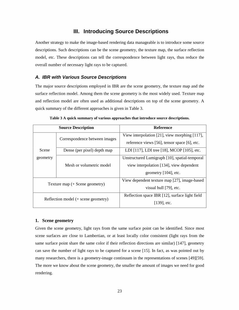
The major source descriptions employed in IBR are the scene geometry, the texture map and the

surface reflection model. Among them the scene geometry is the most widely used. Texture map

and reflection model are often used as additional descriptions on top of the scene geometry. A

quick summary of the different approaches is given in Table 3.

Table 3 A quick summary of various approaches that introduce source descriptions.

Source Description Reference

Correspondence between images View interpolation [21], view morphing [117],

reference views [56], tensor space [6], etc.

Dense (per pixel) depth map LDI [117], LDI tree [18], MCOP [105], etc. Scene

geometry

Mesh or volumetric model

Unstructured Lumigraph [10], spatial-temporal

view interpolation [134], view dependent

geometry [104], etc.

Texture map (+ Scene geometry) View dependent texture map [27], image-based

visual hull [79], etc.

Reflection model (+ scene geometry) Reflection space IBR [12], surface light field

[139], etc.

1. Scene geometry

Given the scene geometry, light rays from the same surface point can be identified. Since most

scene surfaces are close to Lambertian, or at least locally color consistent (light rays from the

same surface point share the same color if their reflection directions are similar) [147], geometry

can save the number of light rays to be captured for a scene [15]. In fact, as was pointed out by

many researchers, there is a geometry-image continuum in the representations of scenes [49][59].

The more we know about the scene geometry, the smaller the amount of images we need for good

rendering.

24

The scene geometry can be described in different forms, such as correspondence between

images (e.g., optical flow), dense depth map, volumetric or mesh model, etc. In this subsection

we classify the various approaches based on different geometry forms they take and present them

one by one.

Correspondence between images

Any scene geometry information can be considered as knowledge about the correspondence

between images. Here we specifically mean approaches that do not have an explicit geometry

representation. Examples of such knowledge are point feature correspondences, disparity map,

optical flow, etc. The idea is to find corresponding light rays in the captured image set for those in

the novel view. In the photogrammetric community, such approaches are developed under the

name of transfer methods.

Early work on this track was under the study of image morphing [7] and often involves

certain manual help. For example, an animator needs to specify a set of feature correspondences,

which form a control mesh. In [138], the novel view is generated by warping the control mesh

through spline interpolation. A two-dimensional free-form deformation and Bézier Clipping was

used to fulfill the same task in [92]. In [7], Beier and Neely defined a global transform/warping

between the two images based on a set of matched line segments. For any view in between, the

matched line segments in the novel view are first interpolated, which then determines the

transform from one of the reference views to the novel view. A deformable surface model based

morphing strategy that does not require the control mesh structure was also discussed in [58].

Recently, a feature-based light field morphing algorithm was proposed in [155].

View interpolation [21], proposed by Chen and Williams, eliminates the need of the human

animator. Instead, the optical flow between the two images is assumed as known. To generate an

in-between view of the input image pair, the offset vectors in the optical flow are linearly

interpolated and the pixels in the source images are moved by the interpolated vector to their

destinations in the novel view. View interpolation performs very well if the two input images are

close to each other, so that visibility ambiguity is not an issue. On the other hand, the interpolated

views will be physically exact only if the camera motion is perpendicular to the camera viewing

axis. In [135] a mathematical formulation was given to show the conditions when linear

interpolation is physically correct.

In [116][117], Seitz and Dyer proposed view morphing. View morphing guarantees that the

rendered view is physically valid by introducing a prewarping stage and a postwarping stage.

During the prewarping, the two reference images are rectified [44]. After the rectification, the two

images share the same image plane and their motion becomes perpendicular to their viewing axis.

25

Linear interpolation is then used to get the intermediate view, followed by postwarping to

compensate the rectification effect on that view.

The novel view in view interpolation and view morphing are often in between the two

reference images. Laveau and Faugeras [56] first proposed to make use of the epipolar constraints

[44], which enabled extrapolation. The novel view is generated from a set of weakly or fully

calibrated reference views. The viewpoint and the retinal plane of the novel view are specified by

manually selected four corresponding points. A dense disparity map is also assumed to be

available. To render the novel view, a ray-tracing like algorithm is implemented, which for each

rendered light ray find the corresponding light rays in the reference views through the epipolar

constraint and the disparity map. Notice that when the reference views are weakly calibrated, only

projective structure can be recovered [44], thus the resultant novel view may appear warped.

Knowing the intrinsic parameters of the cameras (full calibration) will solve such problem.

In plenoptic modeling [82], a similar approach was proposed. The difference is that the

reference view positions are known, and the reference views are now cylindrically projected

panoramic views. Therefore, cylindrical epipolar constraints and dense angular disparity maps

were used for novel view interpolation.

Ref. Image 1 Ref. Image 2

Ref. Image 3Novel view

Seed tensorUnknown tensor

TR,

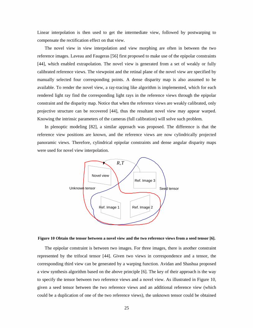
Figure 10 Obtain the tensor between a novel view and the two reference views from a seed tensor [6].

The epipolar constraint is between two images. For three images, there is another constraint

represented by the trifocal tensor [44]. Given two views in correspondence and a tensor, the

corresponding third view can be generated by a warping function. Avidan and Shashua proposed

a view synthesis algorithm based on the above principle [6]. The key of their approach is the way

to specify the tensor between two reference views and a novel view. As illustrated in Figure 10,

given a seed tensor between the two reference views and an additional reference view (which

could be a duplication of one of the two reference views), the unknown tensor could be obtained

26

by knowing the rotation and translation between the third reference view and the novel view.

Therefore specification of a novel view is more direct compared with the epipolar constraint

based methods such as [56], where manual selection of matching points is needed. Moreover,

trifocal tensor based method is often more stable than the epipolar constraint based ones under

certain singular camera configurations (e.g., when the camera centers are collinear).

In a recent approach Lhuillier and Quan [63] presented an interpolation algorithm based on

joint view triangulation. Starting from some points of interest selected automatically, they first

grow the matching points to their neighborhoods. Planar patches are then fit locally for

regularization or removing outliers assuming the matching is piecewise smooth. The two

reference views are then triangulated jointly. Novel views are interpolated by warping the

matched triangles. A walk-through system based on a similar framework was also developed in

[3].

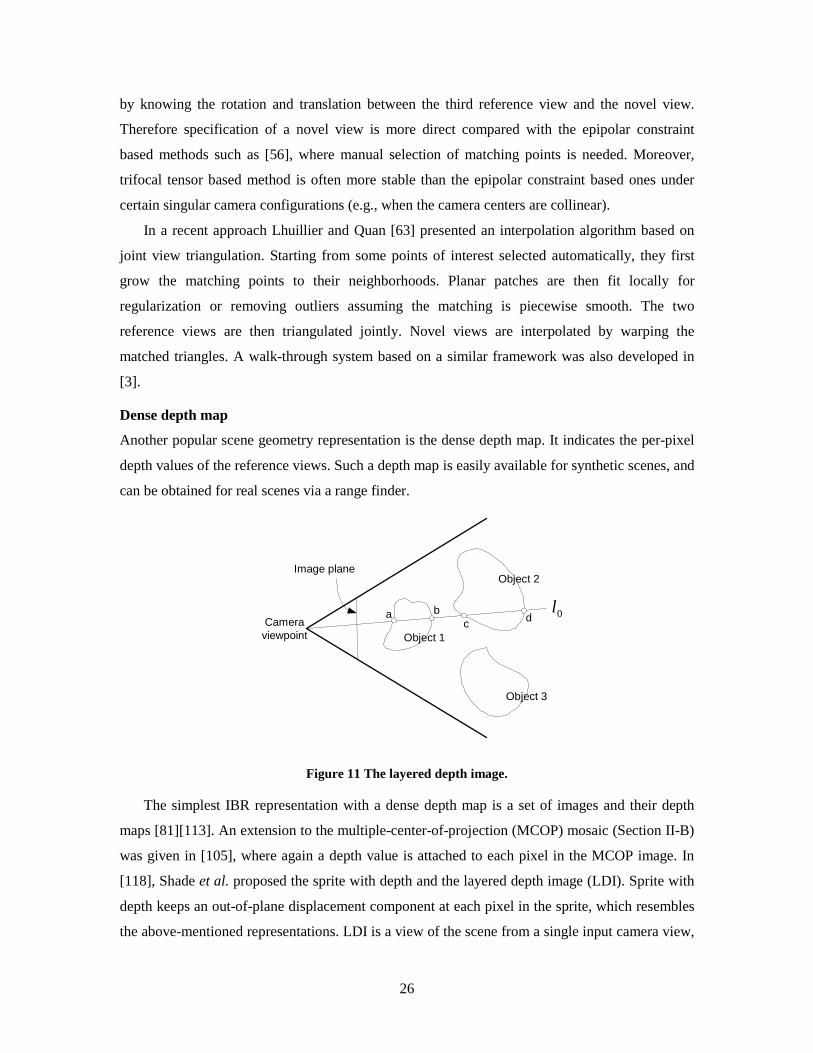
Dense depth map

Another popular scene geometry representation is the dense depth map. It indicates the per-pixel

depth values of the reference views. Such a depth map is easily available for synthetic scenes, and

can be obtained for real scenes via a range finder.

Cameraviewpoint Object 1

Object 3

Object 2Image plane

a bc d 0l

Figure 11 The layered depth image.

The simplest IBR representation with a dense depth map is a set of images and their depth

maps [81][113]. An extension to the multiple-center-of-projection (MCOP) mosaic (Section II-B)

was given in [105], where again a depth value is attached to each pixel in the MCOP image. In

[118], Shade et al. proposed the sprite with depth and the layered depth image (LDI). Sprite with

depth keeps an out-of-plane displacement component at each pixel in the sprite, which resembles

the above-mentioned representations. LDI is a view of the scene from a single input camera view,

27

but with multiple pixels along each line of sight. Correspondingly, the depth map is also multi-

valued for each pixel. This is shown in Figure 11. On the path of the light ray 0l , the depth and

color value of point a, b, c and d are all recorded. Extensions to the LDI include the layered depth

cube [69] and the LDI tree [18].

The rendering algorithms of IBR representations with dense depth map are often similar to

each other. In [81], a 3D warping algorithm was proposed to render novel views that are close to

a reference view. The pixels of the reference view are first projected back to their 3D locations

and then re-projected to the novel view. To speed up the above process, Oliveira and Bishop [95]

proposed to factorize the warping process into a simple pre-warping stage followed by a standard

texture mapping. The pre-warp handles only the parallax effects resulting from the depth map and

the direction of view. The subsequent texture-mapping operation handles the scaling, rotation,

and remaining perspective transformation, which can be accelerated by standard graphics

hardware. A similar factoring algorithm was performed for the LDI [118], where the depth map is

first warped to the output image with visibility check, and colors are pasted afterwards.

One major problem in the above rendering methods is that holes may occur in the rendered

view due to undersampling or disocclusion (scene is occluded in the reference view but visible in

the novel view). By introducing multiple depth values along a light ray, the disocclusion problem

is partially solved in the LDI representation [118]. In [113], because multiple images are available

for rendering, holes due to disocclusion are also not serious as long as the number of images is

large enough. The undersampling problem can also be solved by taking more images. The LDI

tree [18] is a modified LDI approach which combines multiple reference views in to a single

hierarchical representation, which maintains the resolution of each reference view in the data

structure. On the other hand, even if holes do happen, they may be removed through algorithms

such as splatting [78][118] or meshing [78][105].

Mesh or volumetric model

Mesh model is the most widely used components in model-based rendering. Despite the difficulty

to obtain such a model, if it is available in image-based rendering, we should make use of it to

improve the rendering quality.

Buchler et al. proposed the unstructured Lumigraph rendering [10], which addressed the

above rendering problem. They first proposed eight goals for IBR rendering: use of geometric

proxies; unstructured input; epipole consistency; minimal angular deviation; continuity;

resolution sensitivity; equivalent ray consistency and real-time. These goals served as the

guidelines of their proposed unstructured Lumigraph rendering approach. Weighted light ray

interpolation was used to obtain light rays in the novel view. The weights are largely determined

28

by how good the reference light ray is to the interpolated one according to the goals. A clever

weight blending field for the reference views is described to guarantee real-time rendering.

For real-world scenes, the geometry model we reconstruct is often in a volumetric form

[37][134][115][32]. Although the volumetric model can be easily converted to a mesh model

[70], sometimes it may be preferable to render with the volumetric model directly. The algorithm

in [10] can be applied straightforwardly without any change. One concern about the volumetric

model is that it has a finite resolution. To remove the granular effects in the rendered image due

to finite resolution, in [134] a model smoothing algorithm was applied during the rendering,

which greatly improved the resultant image quality.

Rademacher proposed an interesting approach called view dependent geometry [104].

Namely, the geometry used during the rendering may vary when the view position changes. Such

approach is attractive for scenes where the geometry reconstruction algorithm can only obtain a

model that is locally applicable, such as those obtained through stereo methods [111].

Image-based modeling

Scene geometry can often greatly improve the rendering quality, but acquiring the geometry is

not a trivial task unless the scene is synthetic or a range finder is on hand. When no geometry is

directly available, we may resort to computer vision techniques to reconstruct the scene geometry

based on the captured images. Such techniques are called image-based modeling. Due to the close

coupling of image-based rendering and image-based modeling, we see a clear convergence of the

graphics community and the vision community [59].

As a survey of the various image-based modeling techniques is out of the scope of this paper,

we refer the reader to the survey paper by Zhang [156] and by Oliveira [94] for more information.

2. Texture map (+ scene geometry)

Texture map is one of the most widely used source descriptions in model-based rendering. As

texture maps are often obtained from real objects, a geometric model with texture mapping can

produce very realistic scenes.

In image based rendering, when the scene geometry is available, it is possible to generate

texture maps from the reference views. This has already been demonstrated in the 3D warping

algorithm [81] for IBR representations with dense depth map mentioned before. Notice that in

IBR we do not apply reflection models of the scene surface as we do in model-based rendering. A

scene becomes Lambertian if both the geometry and the texture map are fixed. Such scenes may

not be highly interesting. It is therefore natural to introduce texture maps that vary when the

viewpoint changes, namely view dependent texture mapping (VDTM) [27].

29

In [27], Debevec et al. proposed to project the reference views onto the geometric model to

form the texture map through a weighting scheme. The weights are determined by the angular

deviation from the reference views to the virtual view to be rendered. Later a more efficient

implementation of VDTM was proposed in [29], where the per-pixel weight calculation was

replaced by a per-polygon search in a pre-computed lookup table. Note that VDTM is in fact a

special case of the later proposed unstructured Lumigraph rendering [10].

The image-based visual hull (IBVH) algorithm [79] can be considered as another example of

VDTM. In IBVH, the scene geometry was reconstructed through an image space visual hull [57]

algorithm. A texture pixel was generated from the reference views by back projection using only

the light ray with the smallest angular deviation. Such adaptation is partially due to the fact that

only four cameras were used in IBVH.

3. Reflection models (+ scene geometry)

Other than the texture map, the appearance of an object is also determined by the interaction of

the light sources in the environment and the surface reflection model. This becomes more obvious

if the texture map is very simple (e.g., uniform color) and the object is highly specular, such as a

simple mirror ball.

In image-based rendering, we often do not try to figure out what the scene object’s reflection

model is. Instead, we capture light rays that are reflected from the scene surface. Recall that such

parameterization has been discussed under the name surface plenoptic function [149] in Section

II-B. The advantages of recording only the reflected light rays are numerous: we do not need to

derive the underlying surface reflection model any more; we do not need to model the complex

light sources in a real environment; and we do not need to calculate the interaction between the

light source and the reflection model. The downside is that the light source and the reflection

model are now tightly coupled. Efforts need to be made for relighting the scene under different

lighting conditions [141][26].

In [12], Cabral et al. proposed reflection space image-based rendering. Reflection space IBR

records the total reflected radiance for each possible surface direction. Note the difference

between such a radiance environment map and the traditional environment map, where the

incoming radiance is stored [8][39]. The proposed radiance environment map is viewpoint

dependent, thus a set of such maps are pre-computed before rendering, as the multiple images we

often have in normal IBR representations. During the rendering, the radiance environment map is

first interpolated/warped to the desired viewpoint and then used for novel view generation. An

interesting application of radiance environment map is given in [25], where synthetic objects are

rendered into real scenes. A probing mirror ball is used to obtain the radiance environment map at

30

the position the synthetic objects are located. A differential rendering technique allows for good

results to be obtained when only an estimate of the local scene reflectance properties is known.

The above method assumes that if two surface points share the same surface direction, they

have the same reflection pattern. This might not be true due to multiple reasons such as inter-

reflections. A more general approach is to really capture the scene reflections at arbitrary surface

points as in the surface plenoptic function [149]. By ignoring the time and the wavelength

dimensions, Wood et al. proposed surface light field [139]. They first obtained a base mesh of the

scene object through a range scanner. For points on the base mesh, they obtained the reflections

along different directions by capturing hundreds of images of the scene. A pointwise fairing

algorithm was proposed to resample the irregular sample light rays into a reflection map or

lumisphere with a piecewise linear model. Notice that these lumispheres may have missing data

as only light rays reflected to the outside of the object can be captured. Rendering surface light

field is as straightforward as tracing each rendered light ray onto the geometric model and obtain

its radiance. A more compact representation of surface light field suitable for an accelerated

graphics pipeline was recently proposed in [22]. A surface light field created on the surface of a

visual hull rather than the true scene geometry is discussed in [80]. As we mentioned earlier in

Section II-A, under Assumption 2 (the radiance of a light ray does not change along its path in

empty space), using the visual hull surface for recording the light rays is equivalent to using the

true scene geometry as long as the viewpoint is outside the visual hull.

As mentioned before, the surface plenoptic function captures the scene only at a fixed

lighting condition. Recently there has been some work on the relighting of IBR, such as the

human face reflectance field [26], the plenoptic illumination function [141] and the reflected

irradiance field [67]. These approaches share similar ideas. Images of the scene under different

point light source or directional light source are first captured. These images can then be

superimposed to render scenes under a much more complex lighting environment. Such operation

can be performed to live-action scenes in real time [28].

B. Sampling

When certain source description is available, the number of images required is dramatically

reduced. Most of the work listed in this section considered the set of reference images as granted

and tried to render the scene in the best effort. However, it is still interesting to know how many

images we really need for capturing a scene. The problem is in fact much harder than the one

discussed in Section II-C for several reasons. First, the sampling rate will certainly be affected by

how much source description is known and how good the knowledge is. Second, the rendering

31

algorithms used in this section are much more difficult to analysis due to the introduction of many

assumptions and heuristics. How true these assumptions are will also affect the sampling rate.

Last, images used in the IBR representations in this section are usually non-uniformly distributed.

Work in [15][149] is not easily extendable to non-uniform sampling analysis.

Uniform sampling with known scene descriptions

We first discuss several approaches that perform uniform sampling with known scene description.

In [15], a minimum sampling curve was proposed in the joint image and geometry space for light

field. Recall the conclusion in Section II-C that a Lambertian scene at constant depth corresponds

to a tilted line in the frequency domain. If the scene geometry is represented via dense depth map

and each depth value has a finite precision (a certain number of bits), we may divide the scene

into multiple layers based on the depth values. If occlusions between layers are ignored, each

layer can be sampled and rendered independently. This is equivalent to having many scenes with

much smaller depth variation, which reduces the number of images required. An example

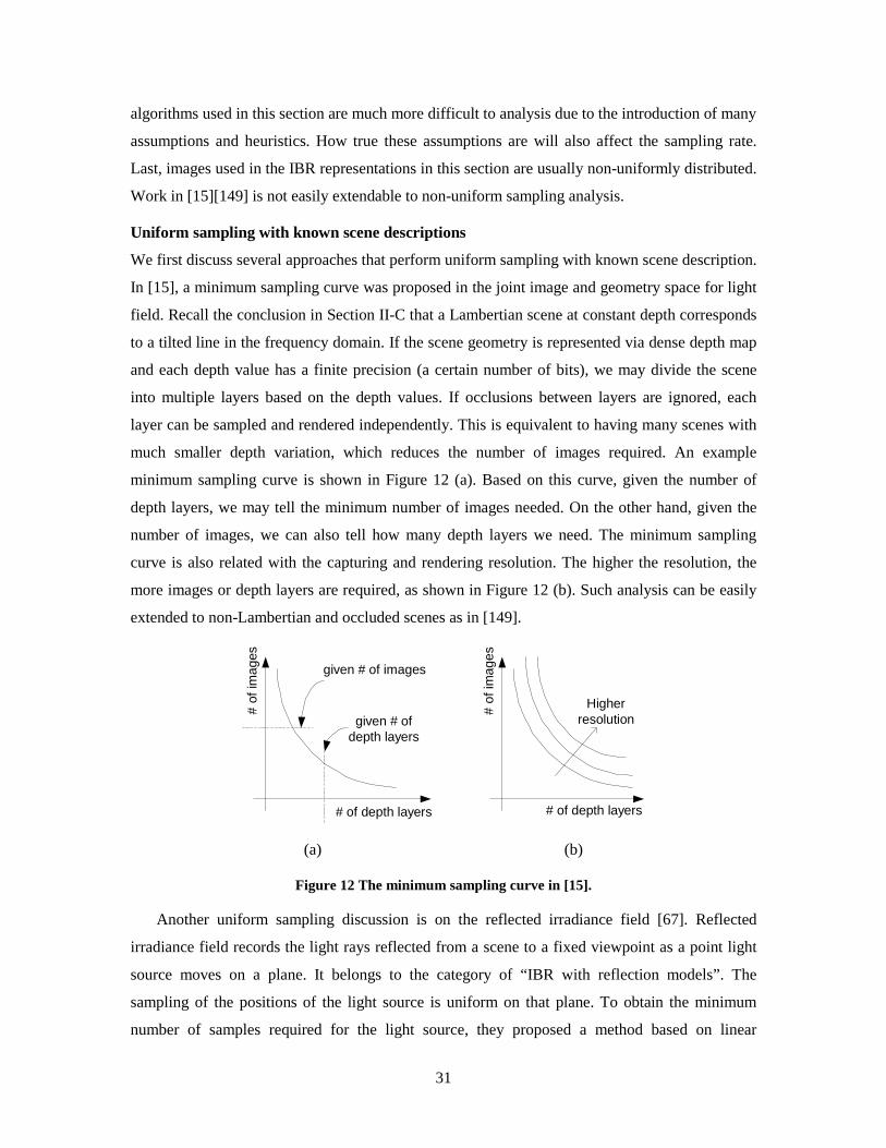
minimum sampling curve is shown in Figure 12 (a). Based on this curve, given the number of

depth layers, we may tell the minimum number of images needed. On the other hand, given the

number of images, we can also tell how many depth layers we need. The minimum sampling

curve is also related with the capturing and rendering resolution. The higher the resolution, the

more images or depth layers are required, as shown in Figure 12 (b). Such analysis can be easily

extended to non-Lambertian and occluded scenes as in [149].

# of depth layers

# of

imag

es

given # of images

given # ofdepth layers

Higherresolution

# of depth layers

# of

imag

es

(a) (b)

Figure 12 The minimum sampling curve in [15].

Another uniform sampling discussion is on the reflected irradiance field [67]. Reflected

irradiance field records the light rays reflected from a scene to a fixed viewpoint as a point light

source moves on a plane. It belongs to the category of “IBR with reflection models”. The

sampling of the positions of the light source is uniform on that plane. To obtain the minimum

number of samples required for the light source, they proposed a method based on linear

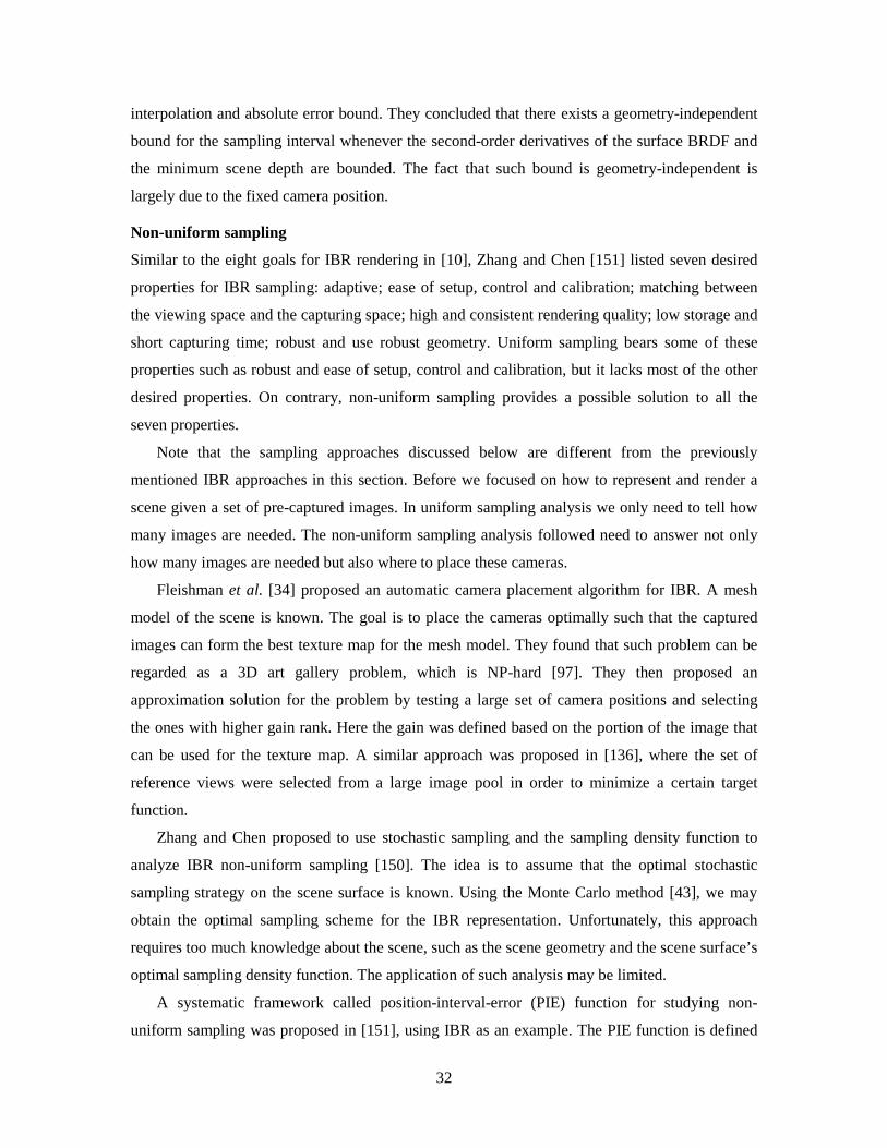
32

interpolation and absolute error bound. They concluded that there exists a geometry-independent

bound for the sampling interval whenever the second-order derivatives of the surface BRDF and

the minimum scene depth are bounded. The fact that such bound is geometry-independent is

largely due to the fixed camera position.

Non-uniform sampling

Similar to the eight goals for IBR rendering in [10], Zhang and Chen [151] listed seven desired

properties for IBR sampling: adaptive; ease of setup, control and calibration; matching between

the viewing space and the capturing space; high and consistent rendering quality; low storage and

short capturing time; robust and use robust geometry. Uniform sampling bears some of these

properties such as robust and ease of setup, control and calibration, but it lacks most of the other

desired properties. On contrary, non-uniform sampling provides a possible solution to all the

seven properties.

Note that the sampling approaches discussed below are different from the previously

mentioned IBR approaches in this section. Before we focused on how to represent and render a

scene given a set of pre-captured images. In uniform sampling analysis we only need to tell how

many images are needed. The non-uniform sampling analysis followed need to answer not only

how many images are needed but also where to place these cameras.

Fleishman et al. [34] proposed an automatic camera placement algorithm for IBR. A mesh

model of the scene is known. The goal is to place the cameras optimally such that the captured

images can form the best texture map for the mesh model. They found that such problem can be

regarded as a 3D art gallery problem, which is NP-hard [97]. They then proposed an

approximation solution for the problem by testing a large set of camera positions and selecting

the ones with higher gain rank. Here the gain was defined based on the portion of the image that

can be used for the texture map. A similar approach was proposed in [136], where the set of

reference views were selected from a large image pool in order to minimize a certain target

function.

Zhang and Chen proposed to use stochastic sampling and the sampling density function to

analyze IBR non-uniform sampling [150]. The idea is to assume that the optimal stochastic

sampling strategy on the scene surface is known. Using the Monte Carlo method [43], we may

obtain the optimal sampling scheme for the IBR representation. Unfortunately, this approach

requires too much knowledge about the scene, such as the scene geometry and the scene surface’s

optimal sampling density function. The application of such analysis may be limited.

A systematic framework called position-interval-error (PIE) function for studying non-

uniform sampling was proposed in [151], using IBR as an example. The PIE function is defined

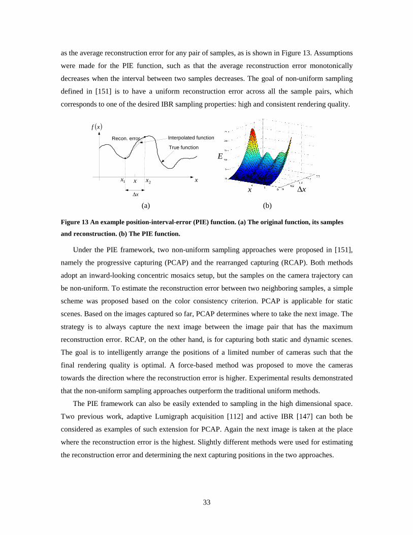
33

as the average reconstruction error for any pair of samples, as is shown in Figure 13. Assumptions

were made for the PIE function, such as that the average reconstruction error monotonically

decreases when the interval between two samples decreases. The goal of non-uniform sampling

defined in [151] is to have a uniform reconstruction error across all the sample pairs, which

corresponds to one of the desired IBR sampling properties: high and consistent rendering quality.

x

x∆

x

( )xf

1x 2x

True function

Interpolated functionRecon. error

x x∆

E

x x∆

E

(a) (b)

Figure 13 An example position-interval-error (PIE) function. (a) The original function, its samples

and reconstruction. (b) The PIE function.

Under the PIE framework, two non-uniform sampling approaches were proposed in [151],

namely the progressive capturing (PCAP) and the rearranged capturing (RCAP). Both methods

adopt an inward-looking concentric mosaics setup, but the samples on the camera trajectory can

be non-uniform. To estimate the reconstruction error between two neighboring samples, a simple

scheme was proposed based on the color consistency criterion. PCAP is applicable for static

scenes. Based on the images captured so far, PCAP determines where to take the next image. The

strategy is to always capture the next image between the image pair that has the maximum

reconstruction error. RCAP, on the other hand, is for capturing both static and dynamic scenes.

The goal is to intelligently arrange the positions of a limited number of cameras such that the

final rendering quality is optimal. A force-based method was proposed to move the cameras

towards the direction where the reconstruction error is higher. Experimental results demonstrated

that the non-uniform sampling approaches outperform the traditional uniform methods.

The PIE framework can also be easily extended to sampling in the high dimensional space.

Two previous work, adaptive Lumigraph acquisition [112] and active IBR [147] can both be

considered as examples of such extension for PCAP. Again the next image is taken at the place

where the reconstruction error is the highest. Slightly different methods were used for estimating

the reconstruction error and determining the next capturing positions in the two approaches.

34

Non-uniform sampling will inevitably increase the complexity of the capturing system in real

applications. However building such systems is still possible, such as the simple PCAP system in

[146].

C. Compression

The compression of IBR representations with source descriptions in this section has not been

widely studied in the literature. However, most of the compression algorithms described in

Section II-D can be directly applied for compressing the reference images. On the other hand,

there are still the source descriptions needed to be compressed other than the images.

In [53] Krishnamurthy et al. considered the compression of depth maps in IBR. Depth map

compression is different from traditional image compression because the compression error has

different impact on the perceived visual quality. In a depth map, certain regions may be more

crucial to the final rendering quality compared to others. For example, they observed that sharp

discontinuities in depth and intensity require more accurate depth maps. Accordingly, a region-of-

interesting (ROI) based coding scheme was proposed. Also, they found that depth error is more

sensitive for closer scene objects and proposed to reshape the dynamic range of the depth image

before compression. This observation coincides with the conclusion in [15], which said that the

depth quantization should be performed in the disparity space rather than the depth space. A

JPEG2000 encoder [127] was used in [53] after the preprocessing.

Duan and Li proposed an algorithm for compressing LDI data [30]. Different from normal

image or depth map, in LDI each pixel is associated with multiple colors and depth values. The

data were organized layer by layer based on how far the scene is from the viewpoint. One key

issue is that for a farther layer, the color and depth map are very sparse. They proposed to

aggregate the data first and then perform compression. High compression ratio at about 10:1 to

20:1 was achieved.

For the compression of other geometric models such as mesh models, there have been many

approaches in the literature. We refer the reader to [126] for a detailed introduction on geometry

compression.

For representations that records the reflected light rays from the scene surface, compression is

also desired. In [139], along with the proposed surface light field, Wood et al. also proposed two

methods to compress the lumispheres, namely function quantization and principal function

analysis. Function quantization resembles the traditional vector quantization, and principal

function analysis is a generalization to the principle component analysis (PCA). These

generalizations are mainly for the purpose of handling the missing data in the lumispheres. In the

35

light field mapping [22], Chen et al. proposed another compression approach that relies on PCA,

VQ and S3 texture compression (S3TCTM) [109]. Since real-time rendering was their goal, many

decisions made in [22] are due to speed concerns. Compression of the plenoptic illumination

function was also discussed in [141] using spherical harmonic transform [24], VQ and DCT.

IV. Conclusions and Future Work

We have surveyed the field of image-based rendering including its representations, sampling and

compression. We found that all the IBR representations are originated from the 7D plenoptic

function, which describes the appearance of the world. As the 7D plenoptic function has too

many data to handle, various approaches were proposed to reduce the data size while still give the

viewer a good browsing experience. Two major strategies were adopted: restraining the viewing

space and introducing source descriptions. We have presented the various IBR representations

based on such categorization. Sampling and compression were discussed separately for the two

strategies, as different strategies results in different representations and thus different sampling

and compression methods.

It is always exciting to predict some of the future directions for IBR. In terms of

representation, IBR through restraining the viewing space is more and more widely adopted in the

real world. For example, many websites now provide virtual tour to their place, among which

most are based on panoramic images. It is expectable that panoramic videos will be an attractive

approach to virtual touring for many resorts. Immersive TV recently receives much attention and

is considered as the next generation of TV technology [33]. Other applications include online

game, remote education, e-commerce, virtual museum, virtual reality/chat room, etc. The key to

the success of IBR representations through restraining the viewing space in the future is the

relaxation of these constraints. We may count on the rapid increasing of storage and memory

space, as well as the increasing of the Internet bandwidth. More devices may need to be

developed (such as dense camera array) in order to capture large, dynamic scenes.

IBR through introducing source descriptions, on the other hand, still requires more future

work. The key problem is not how to perform the rendering, but how to obtain a good source

description. Take the scene geometry as an example. There have been many geometry

reconstruction algorithms proposed in the computer vision literature. However, few of them are

really robust enough to be applied in practical systems. To solve this problem, either we may

develop some low-cost 3D sensing devices, or we may develop new algorithms that can perform

good source description reconstruction.

36

The rendering process in IBR is usually very fast and can be implemented with software.

However, hardware acceleration will be definitely helpful for future high-resolution IBR

rendering. As most operations in IBR rendering are simple mathematical operations such as linear

interpolation, and most IBR rendering process can be performed in parallel, we expect that such

hardware is not difficult to develop and can dramatically increase the rendering speed.

No matter how much the storage and memory increase in the future, sampling and

compression are always useful to keep the IBR data at a manageable size. The work on sampling

and compression, however, has just started. There are still many problems remain unsolved, such

as the sampling rate when certain source description is available. A high compression ratio in IBR

seems rely heavily on how good the images can be predicted, which depends on, e.g., how good a

certain source description can be reconstructed. Joint work between the signal processing

community and the computer vision community is highly expected.

Image-based rendering is still an emerging field. From this survey, it is obvious that IBR has

attracted many researchers from various communities, including computer graphics, computer

vision and signal processing. We believe that the cooperation of different communities will

certainly bring a bright future for IBR.

Reference

[1] 360 One VRTM, Kaidan, http://www.kaidan.com/.

[2] E. H. Adelson, and J. R. Bergen, “The plenoptic function and the elements of early vision”,

Computational Models of Visual Processing, Edited by Michael Landy and J. Anthony Movshon. The MIT

Press, Cambridge, Mass. 1991, Chapter 1.

[3] G. Agarwal, D. Rathi, P. K. Kalra and S. Banerjee, “A System for Image Based Rendering of Walk-

throughs”, Computer Graphics International (CGI2002), Bradford, UK, July 2002.

[4] T. Akenine-Moller and E. Haines, Real-Time Rendering, 2nd Edition, A K Peters Ltd.

[5] D. G. Aliaga and I. Carlbom, “Plenoptic stitching: a scalable method for reconstructing 3D

interactive walkthroughs”, Computer Graphics (SIGGRAPH’01), August 2001, pp. 443-450.

[6] S. Avidan and A. Shashua, “Novel view synthesis in tensor space”, CVPR’97, San Juan, Puerto

Rico, 1997, pp. 1034-1040.

[7] T. Beier and S. Neely, “Feature-Based Image Metamorphosis”, Computer Graphics

(SIGGRAPH’92), July 1992, pp. 35-42.

[8] J. F. Blinn and M. E. Newell, “Texture and Reflection in Computer Generated Images”,

Communications of the ACM, Vol. 19, No. 10, 1976, pp. 542-546.

[9] S. Borman and R. L. Stevenson, “Super-Resolution from Image Sequences - A Review”, Midwest

Symposium on Circuits and Systems, 1998.

37

[10] C. Buehler, M. Bosse, L. McMillan, S. Gortler, and M. Cohen, “Unstructured Lumigraph

rendering”, Computer Graphics (SIG-GRAPH’01), August 2001, pp 425-432.

[11] CBS Broadcasting Inc., http://www.cbs.com.

[12] B. Cabral, M. Olano, P. Nemec, “Reflection space image based rendering”, Computer Graphics

(SIGGRAPH’99), August 1999, pp. 165-171.

[13] E. Camahort and D. Fussell, “A Geometric Study of Light Field Representations”, Technical Report

TR99-35, Department of Computer Sciences, The University of Texas at Austin.

[14] E. Camahort, A. Lerios and D. Fussell, “Uniformly sampled light fields”, 9th Eurographics

Workshop on Rendering, Vienna, Austria, June/July 1998, pp. 117-130.

[15] J.X. Chai, X. Tong, S.C. Chan and H. Y. Shum, “Plenoptic sampling”, Computer Graphics

(SIGGRAPH’00), July 2000, pp. 307-318.

[16] S. C. Chan, K. T. Ng, Z. F. Gan, K. L. Chan and H.-Y. Shum, “The Data Compression of Simplified

Dynamic Light Fields”, ICASSP’03, Hong Kong, Apr. 2003.

[17] S. C. Chan and H. Y. Shum, “A Spectral Analysis for Light Field Rendering”, ICIP’00, Vancouver,

Canada, Sep. 2000.

[18] C. Chang, G. Bishop and A. Lastra, “LDI tree: A hierarchical representation for image-based

rendering”, Computer Graphics (SIGGRAPH’99), August 1999, pp. 291-298.

[19] C.-L. Chang, X. Zhu, P. Ramanathan and B. Girod, “Shape Adaptation for Light Field

Compression”, ICIP’03, Barcelona, Spain, Sep. 2003.

[20] S. E. Chen, “QuickTime VR – An Image-Based Approach to Virtual Environment Navigation”,

Computer Graphics (SIGGRAPH’95), August 1995, pp. 29-38.

[21] S. E. Chen and L. Williams, “View interpolation for image synthesis”, Computer Graphics

(SIGGRAPH’93), August 1993, pp. 279-288.

[22] W.-C. Chen, J.-Y. Bouguet, M. H. Chu, R. Grzeszczuk, “Light field mapping: efficient

representation and hardware rendering of surface light fields”, Computer Graphics (SIGGRAPH’02), July

2002, pp. 447-456.

[23] T. N. Cornsweet, Visual Perception, Academic Press, 1971.

[24] R. Courant and D. Hilbert, Methods of Mathematical Physics, New York: Interscience, 1953.

[25] P. Debevec, “Rendering Synthetic Objects into Real Scenes: Bridging Traditional and Image-Based

Graphics with Global Illumination and High Dynamic Range Photography”, Computer Graphics

(SIGGRAPH’98), Aug. 1998, pp. 189-198.

[26] P. Debevec, T. Hawkins, C. Tchou, H.-P. Duiker, W. Sarokin and M. Sagar, “Acquiring the

Reflectance Field of a Human Face”, Computer Graphics (SIGGRAPH’00), July 2000, pp. 145-156.

[27] P. Debevec, C. J. Taylor and J. Malik, “Modeling and rendering architecture from photographs: a

hybrid geometry- and image-based approach”, Computer Graphics (SIGGRAPH’96), August 1996, pp. 11-

20.

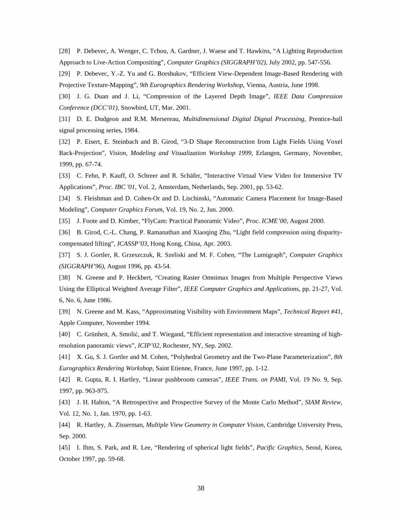
38

[28] P. Debevec, A. Wenger, C. Tchou, A. Gardner, J. Waese and T. Hawkins, “A Lighting Reproduction

Approach to Live-Action Compositing”, Computer Graphics (SIGGRAPH’02), July 2002, pp. 547-556.

[29] P. Debevec, Y.-Z. Yu and G. Borshukov, “Efficient View-Dependent Image-Based Rendering with

Projective Texture-Mapping”, 9th Eurographics Rendering Workshop, Vienna, Austria, June 1998.

[30] J. G. Duan and J. Li, “Compression of the Layered Depth Image”, IEEE Data Compression

Conference (DCC’01), Snowbird, UT, Mar. 2001.

[31] D. E. Dudgeon and R.M. Mersereau, Multidimensional Digital Dignal Processing, Prentice-hall

signal processing series, 1984.

[32] P. Eisert, E. Steinbach and B. Girod, “3-D Shape Reconstruction from Light Fields Using Voxel

Back-Projection”, Vision, Modeling and Visualization Workshop 1999, Erlangen, Germany, November,

1999, pp. 67-74.

[33] C. Fehn, P. Kauff, O. Schreer and R. Schäfer, “Interactive Virtual View Video for Immersive TV

Applications”, Proc. IBC '01, Vol. 2, Amsterdam, Netherlands, Sep. 2001, pp. 53-62.

[34] S. Fleishman and D. Cohen-Or and D. Lischinski, “Automatic Camera Placement for Image-Based

Modeling”, Computer Graphics Forum, Vol. 19, No. 2, Jun. 2000.

[35] J. Foote and D. Kimber, “FlyCam: Practical Panoramic Video”, Proc. ICME’00, August 2000.

[36] B. Girod, C.-L. Chang, P. Ramanathan and Xiaoqing Zhu, “Light field compression using disparity-

compensated lifting”, ICASSP’03, Hong Kong, China, Apr. 2003.

[37] S. J. Gortler, R. Grzeszczuk, R. Szeliski and M. F. Cohen, “The Lumigraph”, Computer Graphics

(SIGGRAPH’96), August 1996, pp. 43-54.

[38] N. Greene and P. Heckbert, “Creating Raster Omnimax Images from Multiple Perspective Views

Using the Elliptical Weighted Average Filter”, IEEE Computer Graphics and Applications, pp. 21-27, Vol.

6, No. 6, June 1986.

[39] N. Greene and M. Kass, “Approximating Visibility with Environment Maps”, Technical Report #41,

Apple Computer, November 1994.

[40] C. Grünheit, A. Smolić, and T. Wiegand, “Efficient representation and interactive streaming of high-

resolution panoramic views”, ICIP’02, Rochester, NY, Sep. 2002.

[41] X. Gu, S. J. Gortler and M. Cohen, “Polyhedral Geometry and the Two-Plane Parameterization”, 8th

Eurographics Rendering Workshop, Saint Etienne, France, June 1997, pp. 1-12.

[42] R. Gupta, R. I. Hartley, “Linear pushbroom cameras”, IEEE Trans. on PAMI, Vol. 19 No. 9, Sep.

1997, pp. 963-975.

[43] J. H. Halton, “A Retrospective and Prospective Survey of the Monte Carlo Method”, SIAM Review,

Vol. 12, No. 1, Jan. 1970, pp. 1-63.

[44] R. Hartley, A. Zisserman, Multiple View Geometry in Computer Vision, Cambridge University Press,

Sep. 2000.

[45] I. Ihm, S. Park, and R. Lee, “Rendering of spherical light fields”, Pacific Graphics, Seoul, Korea,

October 1997, pp. 59-68.

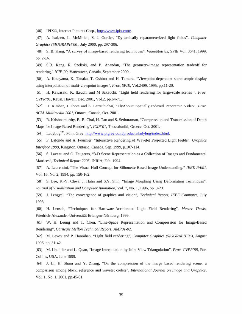
39

[46] IPIX®, Internet Pictures Corp., http://www.ipix.com/.

[47] A. Isaksen, L. McMillan, S. J. Gortler, “Dynamically reparameterized light fields”, Computer

Graphics (SIGGRAPH’00), July 2000, pp. 297-306.

[48] S. B. Kang, “A survey of image-based rendering techniques”, VideoMetrics, SPIE Vol. 3641, 1999,

pp. 2-16.

[49] S.B. Kang, R. Szeliski, and P. Anandan, “The geometry-image representation tradeoff for

rendering,” ICIP’00, Vancouver, Canada, September 2000.

[50] A. Katayama, K. Tanaka, T. Oshino and H. Tamura, “Viewpoint-dependent stereoscopic display

using interpolation of multi-viewpoint images”, Proc. SPIE, Vol.2409, 1995, pp.11-20.

[51] H. Kawasaki, K. Ikeuchi and M Sakauchi, “Light field rendering for large-scale scenes ”, Proc.

CVPR’01, Kauai, Hawaii, Dec. 2001, Vol.2, pp.64-71.

[52] D. Kimber, J. Foote and S. Lertsithichai, “FlyAbout: Spatially Indexed Panoramic Video”, Proc.

ACM Multimedia 2001, Ottawa, Canada, Oct. 2001.

[53] R. Krishnamurthy, B.-B. Chai, H. Tao and S. Sethuraman, “Compression and Transmission of Depth

Maps for Image-Based Rendering”, ICIP’01, Thessaloniki, Greece, Oct. 2001.

[54] LadybugTM, Point Grey, http://www.ptgrey.com/products/ladybug/index.html.

[55] P. Lalonde and A. Fournier, “Interactive Rendering of Wavelet Projected Light Fields”, Graphics

Interface 1999, Kingston, Ontario, Canada, Sep. 1999, p.107-114.

[56] S. Laveau and O. Faugeras, “3-D Scene Representation as a Collection of Images and Fundamental

Matrices”, Technical Report 2205, INRIA, Feb. 1994.

[57] A. Laurentini, “The Visual Hull Concept for Silhouette Based Image Understanding.” IEEE PAMI,

Vol. 16, No. 2, 1994, pp. 150-162.

[58] S. Lee, K.-Y. Chwa, J. Hahn and S.Y. Shin, “Image Morphing Using Deformation Techniques”,

Journal of Visualization and Computer Animation, Vol. 7, No. 1, 1996, pp. 3-23.

[59] J. Lengyel, “The convergence of graphics and vision”, Technical Report, IEEE Computer, July

1998.

[60] H. Lensch, “Techniques for Hardware-Accelerated Light Field Rendering”, Master Thesis,

Friedrich-Alexander-Universität Erlangen-Nürnberg, 1999.

[61] W. H. Leung and T. Chen, “Line-Space Representation and Compression for Image-Based

Rendering”, Carnegie Mellon Technical Report: AMP01-02.

[62] M. Levoy and P. Hanrahan, “Light field rendering”, Computer Graphics (SIGGRAPH’96), August

1996, pp. 31-42.

[63] M. Lhuillier and L. Quan, “Image Interpolation by Joint View Triangulation”, Proc. CVPR’99, Fort

Collins, USA, June 1999.

[64] J. Li, H. Shum and Y. Zhang, "On the compression of the image based rendering scene: a

comparison among block, reference and wavelet coders", International Journal on Image and Graphics,

Vol. 1, No. 1, 2001, pp.45-61.

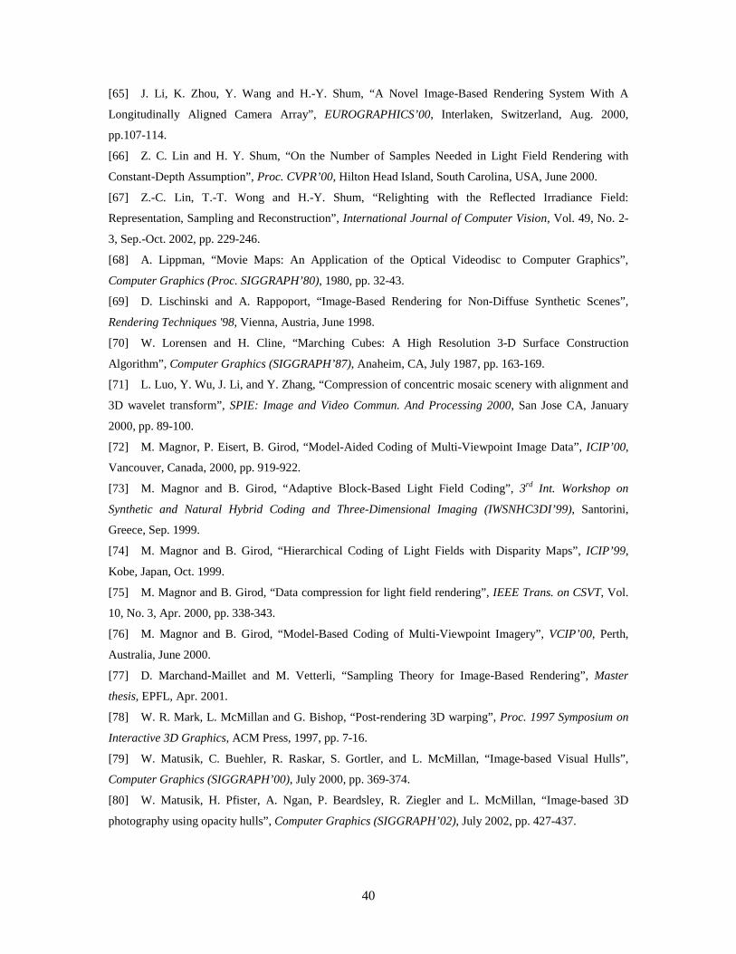
40

[65] J. Li, K. Zhou, Y. Wang and H.-Y. Shum, “A Novel Image-Based Rendering System With A

Longitudinally Aligned Camera Array”, EUROGRAPHICS’00, Interlaken, Switzerland, Aug. 2000,

pp.107-114.

[66] Z. C. Lin and H. Y. Shum, “On the Number of Samples Needed in Light Field Rendering with

Constant-Depth Assumption”, Proc. CVPR’00, Hilton Head Island, South Carolina, USA, June 2000.

[67] Z.-C. Lin, T.-T. Wong and H.-Y. Shum, “Relighting with the Reflected Irradiance Field:

Representation, Sampling and Reconstruction”, International Journal of Computer Vision, Vol. 49, No. 2-

3, Sep.-Oct. 2002, pp. 229-246.

[68] A. Lippman, “Movie Maps: An Application of the Optical Videodisc to Computer Graphics”,

Computer Graphics (Proc. SIGGRAPH’80), 1980, pp. 32-43.

[69] D. Lischinski and A. Rappoport, “Image-Based Rendering for Non-Diffuse Synthetic Scenes”,

Rendering Techniques '98, Vienna, Austria, June 1998.

[70] W. Lorensen and H. Cline, “Marching Cubes: A High Resolution 3-D Surface Construction

Algorithm”, Computer Graphics (SIGGRAPH’87), Anaheim, CA, July 1987, pp. 163-169.

[71] L. Luo, Y. Wu, J. Li, and Y. Zhang, “Compression of concentric mosaic scenery with alignment and

3D wavelet transform”, SPIE: Image and Video Commun. And Processing 2000, San Jose CA, January

2000, pp. 89-100.

[72] M. Magnor, P. Eisert, B. Girod, “Model-Aided Coding of Multi-Viewpoint Image Data”, ICIP’00,

Vancouver, Canada, 2000, pp. 919-922.

[73] M. Magnor and B. Girod, “Adaptive Block-Based Light Field Coding”, 3rd Int. Workshop on

Synthetic and Natural Hybrid Coding and Three-Dimensional Imaging (IWSNHC3DI’99), Santorini,

Greece, Sep. 1999.

[74] M. Magnor and B. Girod, “Hierarchical Coding of Light Fields with Disparity Maps”, ICIP’99,

Kobe, Japan, Oct. 1999.

[75] M. Magnor and B. Girod, “Data compression for light field rendering”, IEEE Trans. on CSVT, Vol.

10, No. 3, Apr. 2000, pp. 338-343.

[76] M. Magnor and B. Girod, “Model-Based Coding of Multi-Viewpoint Imagery”, VCIP’00, Perth,

Australia, June 2000.

[77] D. Marchand-Maillet and M. Vetterli, “Sampling Theory for Image-Based Rendering”, Master

thesis, EPFL, Apr. 2001.

[78] W. R. Mark, L. McMillan and G. Bishop, “Post-rendering 3D warping”, Proc. 1997 Symposium on

Interactive 3D Graphics, ACM Press, 1997, pp. 7-16.

[79] W. Matusik, C. Buehler, R. Raskar, S. Gortler, and L. McMillan, “Image-based Visual Hulls”,

Computer Graphics (SIGGRAPH’00), July 2000, pp. 369-374.

[80] W. Matusik, H. Pfister, A. Ngan, P. Beardsley, R. Ziegler and L. McMillan, “Image-based 3D

photography using opacity hulls”, Computer Graphics (SIGGRAPH’02), July 2002, pp. 427-437.

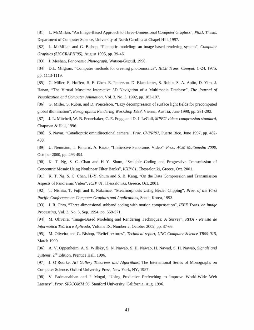
41

[81] L. McMillan, “An Image-Based Approach to Three-Dimensional Computer Graphics”, Ph.D. Thesis,

Department of Computer Science, University of North Carolina at Chapel Hill, 1997.

[82] L. McMillan and G. Bishop, “Plenoptic modeling: an image-based rendering system”, Computer

Graphics (SIGGRAPH’95), August 1995, pp. 39-46.

[83] J. Meehan, Panoramic Photograph, Watson-Guptill, 1990.

[84] D.L. Milgram, “Computer methods for creating photomosaics”, IEEE Trans. Comput. C-24, 1975,

pp. 1113-1119.

[85] G. Miller, E. Hoffert, S. E. Chen, E. Patterson, D. Blackketter, S. Rubin, S. A. Aplin, D. Yim, J.

Hanan, “The Virtual Museum: Interactive 3D Navigation of a Multimedia Database”, The Journal of

Visualization and Computer Animation, Vol. 3, No. 3, 1992, pp. 183-197.

[86] G. Miller, S. Rubin, and D. Ponceleon, “Lazy decompression of surface light fields for precomputed

global illumination”, Eurographics Rendering Workshop 1998, Vienna, Austria, June 1998, pp. 281-292.

[87] J. L. Mitchell, W. B. Pennebaker, C. E. Fogg, and D. J. LeGall, MPEG video: compression standard,

Chapman & Hall, 1996.

[88] S. Nayar, “Catadioptric omnidirectional camera”, Proc. CVPR’97, Puerto Rico, June 1997, pp. 482-

488.

[89] U. Neumann, T. Pintaric, A. Rizzo, “Immersive Panoramic Video”, Proc. ACM Multimedia 2000,

October 2000, pp. 493-494.

[90] K. T. Ng, S. C. Chan and H.-Y. Shum, “Scalable Coding and Progressive Transmission of

Concentric Mosaic Using Nonlinear Filter Banks”, ICIP’01, Thessaloniki, Greece, Oct. 2001.

[91] K. T. Ng, S. C. Chan, H.-Y. Shum and S. B. Kang, “On the Data Compression and Transmission

Aspects of Panoramic Video”, ICIP’01, Thessaloniki, Greece, Oct. 2001.

[92] T. Nishita, T. Fujii and E. Nakamae, “Metamorphosis Using Bézier Clipping”, Proc. of the First

Pacific Conference on Computer Graphics and Applications, Seoul, Korea, 1993.

[93] J. R. Ohm, “Three-dimensional subband coding with motion compensation”, IEEE Trans. on Image

Processing, Vol. 3, No. 5, Sep. 1994, pp. 559-571.

[94] M. Oliveira, “Image-Based Modeling and Rendering Techniques: A Survey”, RITA - Revista de

Informática Teórica e Aplicada, Volume IX, Number 2, October 2002, pp. 37-66.

[95] M. Oliveira and G. Bishop, “Relief textures”, Technical report, UNC Computer Science TR99-015,

March 1999.

[96] A. V. Oppenheim, A. S. Willsky, S. N. Nawab, S. H. Nawab, H. Nawad, S. H. Nawab, Signals and

Systems, 2nd Edition, Prentice Hall, 1996.

[97] J. O’Rourke, Art Gallery Theorems and Algorithms, The International Series of Monographs on

Computer Science. Oxford University Press, New York, NY, 1987.

[98] V. Padmanabhan and J. Mogul, “Using Predictive Prefetching to Improve World-Wide Web

Latency”, Proc. SIGCOMM’96, Stanford University, California, Aug. 1996.

42

[99] S. Peleg and M. Ben-Ezra, “Stereo Panorama with a Single Camera”, Proc. CVPR’99, Ft. Collins,

Colorado, June 1999.

[100] S. Peleg and J. Herman, “Panoramic Mosaics by Manifold Projection”, Proc. CVPR’97,

Washington, June 1997, pp. 338-343.

[101] S. Peleg, B. Rousso, A. Rav-Acha, A. Zomet, “Mosaicing on adaptive manifolds”, IEEE Trans. on

PAMI, Vol. 22 No. 10, Oct 2000, pp. 1144-1154.

[102] T. Ebrahimi and F. Pereira, The MPEG-4 Book, Prentice Hall PTR, July 2002.

[103] I. Peter and W. Straßer, “The Wavelet Stream - Progressive Transmission of Compressed Light Field

Data”, IEEE Visualization 1999, San Francisco, CA.

[104] P. Rademacher, “View-dependent geometry”, Computer Graphics (SIGGRAPH’99), August 1999,

pp. 439-446.

[105] P. Rademacher and G. Bishop, “Multiple-center-of-projection images”, Computer Graphics

(SIGGRAPH’98), August 1998, pp. 199-206.

[106] P. Ramanathan, M. Kalman and B. Girod, “Rate-Distortion Optimized Streaming of Compressed

Light Fields”, ICIP’03, Barcelona, Spain, Sep. 2003.

[107] P. Ramanathan, E. Steinbach, P. Eisert and B. Girod, “Geometry refinement for light field

compression”, ICIP’02, Rochester, NY, Sep. 2002.

[108] D. G. Ripley, “DVI-a Digital Multimedia Technology”, Communications of the ACM, Vol. 32 No. 7,

1989, pp. 811-822.

[109] S3TCTM, SONICblue Incorporated, http://www.s3.com/.

[110] H. S. Sawhney and R. Kumar, “True multi-image alignment and its application to mosaicing and

lens distortion correction”, IEEE Trans. PAMI, Vol. 21 No. 3, Mar. 1999, pp. 235-243.

[111] D. Scharstein and R. Szeliski, “A Taxonomy and Evaluation of Dense Two-Frame Stereo

Correspondence Algorithms”, Int. Journal of Computer Vision, Vol. 47, No. 1/2/3, Apr.-Jun. 2002, pp7-42.

[112] H. Schirmacher, W. Heidrich and H. P. Seidel, “Adaptive Acquisition of Lumigraphs from Synthetic

Scenes”, EUROGRAPHICS’99, Vol. 18, No. 3, 1999.

[113] H. Schirmacher, W. Heidrich and H. P. Seidel. “High-quality interactive Lumigraph rendering

through warping” Graphics Interface 2000, Montreal, Canada, May 2000.

[114] I. O. Sebe, P. Ramanathan and B. Girod, “Multi-View Geometry Estimation for Light Field

Compression”, Proc. Vision, Modeling and Visualization (VMV-2002), Erlangen, Germany, Nov. 2002, pp.

265-272.

[115] S. M. Seitz and C. R. Dyer, “Photorealistic Scene Reconstruction by Voxel Coloring”, Proc.

CVPR’97, San Juan, Puerto Rico, June 1997, pp. 1067-1073.

[116] S. M. Seitz and C. R. Dyer, “Physically-Valid View Synthesis by Image Interpolation”, Proc.

Workshop on Representation of Visual Scenes, 1995, pp. 18-25.

[117] S. M. Seitz and C. M. Dyer, “View morphing”, Computer Graphics (SIGGRAPH’96), August 1996,

pp. 21-30.

43

[118] J. Shade, S. Gortler, L.-W. He and R. Szeliski, “Layered depth images”, Computer Graphics

(SIGGRAPH’98), August 1998, pp. 231-242.

[119] H.-Y. Shum and L.-W. He, “Rendering with concentric mosaics”, Computer Graphics

(SIGGRAPH’99), August 1999, pp.299-306.

[120] H.-Y. Shum, K. T. Ng and S. C. Chan, “Virtual Reality Using the Concentric Mosaic: Construction,

Rendering and Data Compression”, ICIP’00, Vancouver, Canada, Sep. 2000, pp. 644-647.

[121] H.-Y. Shum, L.-F. Wang, J.-X. Chai and X. Tong, “Rendering with Manifold Hopping”,

International Journal of Computer Vision, Vol. 50, No. 2, Nov. 2002, pp. 185-201.

[122] P. P. Sloan, M. F. Cohen and S. J. Gortler, “Time critical Lumigraph rendering”, Symposium on

Interactive 3D Graphics, Providence, RI, USA, 1997, pp.17-23.

[123] R. Swaminathan and S.K. Nayar, “Polycameras: Camera Clusters for Wide Angle Imaging”,

Columbia University Technical Report, CUCS-013-99.

[124] R. Szeliski, “Image Mosaicing for Tele-Reality Applications”, Technical Report CRL94/2, DEC

Cambridge Research Lab, May 1994.

[125] R. Szeliski and H.-Y. Shum, “Creating full view panoramic image mosaics and texture-mapped

models”, Computer Graphics (SIGGRAPH’97), August 1997, pp. 251-258.

[126] G. Taubin and J. Rossignac, Course 38: 3D Geometry Compression, Siggraph'2000 Course Notes,

July 2000.

[127] D. Taubman and M. Marcellin, Jpeg2000: Image Compression Fundamentals, Standards, and

Practice, Kluwer Academic Publishers, Nov. 2001.

[128] D. Taubman and A. Zakhor, “Multirate 3-D subband coding of video”, IEEE Trans. on Image Proc-

essing, Vol. 3, No. 5, Sep. 1994, pp. 572-588.

[129] S. Teller, M. Antone, Z. Bodnar, M. Bosse, S. Coorg, M. Jethwa, N. Master, “Calibrated, Registered

Images of and Extended Urban Area”, to appear in the International Journal of Computer Vision, 2003.

[130] J. Y. Tham, S. Ranganath, and A. A. Kassim, “Highly scalable wavelet-based video codec for very

low bit-rate environment”, IEEE Journal on Selected Areas in Communications, vol. 16, no. 1, Jan. 1998.

[131] X. Tong and R. M. Gray, “Coding of Multi-View Images for Immersive Viewing”, ICASSP’00,

Istanbul, Turkey, vol. 4, June 2000, pp. 1879-1882.

[132] TotalViewTM, Be Here Technologies, http://www.behere.com/.

[133] M. Uyttendaele A. Eden, R. Szeliski, “Eliminating Ghosting and Exposure Artifacts in Image

Mosaics”, Proc. CVPR’01, Kauai, Hawaii, Dec. 2001, pp. 509-516.

[134] S. Vedula, S. Baker and T. Kanade, “Spatio-Temporal View Interpolation”, Proc. of the 13th ACM

Eurographics Workshop on Rendering, June, 2002.

[135] T. Werner, R. D. Hersch and V. Hlavác, “Rendering Real-World Objects Using View Interpolation”,

Proc. ICCV’95, Boston, MA, June 1995.

[136] T. Werner, V. Hlavác, A. Leonardis and T. Pajdla, “Selection of Reference Views for Image-Based

Representation”, Proc. ICPR’96, Vienna, Austria, Aug. 1996, pp.73-77.

44

[137] B. Wilburn, M. Smulski, H.-H. K. Lee and M. Horowitz, “The Light Field Video Camera”,

Proceedings of Media Processors 2002, SPIE Electronic Imaging 2002.

[138] G. Wolberg, Digital Image Warping, IEEE Computer Society Press, 1990.

[139] D. N. Wood, D. I. Azuma, K. Aldinger, B. Curless, T. Duchamp, D. H. Salesin and W. Stuetzle,

“Surface light fields for 3D photography”, Computer Graphics (SIGGRAPH’00), July 2000, pp. 287-296.

[140] D. N. Wood, A. Finkelstein, J. F. Hughes, C. E. Thayer and D. H. Salesin, “Multiperspective

panoramas for cel animation”, Computer Graphics (SIGGRAPH’97), August 1997, pp.243-250.

[141] T.-T. Wong, C. W. Fu, P.-A. Heng and C.-S. Leung, “The Plenoptic Illumination Function”, IEEE

Trans. on Multimedia, Vol. 4, No. 3, Sep. 2002, pp. 361-371.

[142] Y. Wu, L. Luo, J. Li and Y. Zhang, “Rendering of 3D Wavelet Compressed Concentric Mosaic

Scenery with Progressive Inverse Wavelet Synthesis (PIWS)”, VCIP’00, Perth, Australia, June 2000.

[143] Y. Wu, C. Zhang and J. Li, “Smart-Rebinning for Compression of Concentric Mosaic”, IEEE Trans.

on Multimedia, Vol. 4, No. 3, Sep. 2002, pp 332-342.

[144] Y. Xiong and K. Turkowski, “Creating image-based VR using a self-calibration fisheye lens”, Proc.

CVPR’97, Puerto Rico, June 1997, pp. 237-243.

[145] J. C. Yang, M. Everett, C. Buehler and L. McMillan, “A Real-Time Distributed Light Field

Camera”, Eurographics Workshop on Rendering 2002, pp. 1-10.

[146] C. Zhang and T. Chen, “A System for Active Image-Based Rendering”, ICME’03, Baltimore,

Maryland, July 2003.

[147] C. Zhang and T. Chen, “Active Scene Capturing for Image-Based Rendering”, Carnegie Mellon

Technical Report: AMP03-02.

[148] C. Zhang and T. Chen, “Generalized Plenoptic Sampling”, Carnegie Mellon Technical Report:

AMP01-06.

[149] C. Zhang and T. Chen, “Spectral Analysis for Sampling Image-Based Rendering Data”, to appear in

IEEE Trans. on CSVT, Special Issue on Image-based Modeling, Rendering and Animation.

[150] C. Zhang and T. Chen, “Surface Plenoptic Function as a Tool for Image-Based Rendering Sampling

Analysis”, ICASSP’03, Hong Kong, China, April 2003.

[151] C. Zhang and T. Chen, “Non-Uniform Sampling of Image-Based Rendering Data with the Position-

Interval-Error (PIE) Function”, VCIP’03, Lugano, Switzerland, July 2003.

[152] C. Zhang and J. Li, “Compression of Lumigraph with Multiple Reference Frame (MRF) Prediction

and Just-In-Time Rendering," Proc. IEEE Data Compression Conf. (DCC'00), Snowbird, Utah, March

2000, pp. 254-263.

[153] C. Zhang and J. Li, “Compression and Rendering of Concentric Mosaics with Reference Block

Codec (RBC)”, VCIP'00, Perth, Australia, June 2000.

[154] C. Zhang and J. Li, “Interactive Browsing of 3D Environment over the Internet”, VCIP’01, San Jose,

CA, Jan. 2001.

45

[155] Z.-P. Zhang, L.-F. Wang, B.-N. Guo, H.-Y. Shum, “Feature-based light field morphing”, Computer

Graphics (SIGGRAPH’02), July 2002, pp. 457-464.

[156] Z.-Y. Zhang, “Image-based geometrically-correct photorealistic scene / object modeling (IBPhM): a

review”, Asian Conference on Computer Vision (ACCV’98), Hong Kong, Jan. 8-11, 1998.

[157] J. Y. Zheng and S. Tsuji, “Panoramic Representation of Scenes for Route Understanding”, Proc.

ICPR’90, June 1990, pp. 161-167.