a study of information-theoretic metaheuristics applied to ... · a study of information-theoretic...
TRANSCRIPT

A study of information-theoretic
metaheuristics applied to functional
neuroimaging datasets
Extracting characteristic textures from fMRI data taken during
a visual contour-integration task
Inaugural-Dissertation zur Erlangung der Doktorwürde
der Fakultät für Sprach-, Literatur- und Kulturwissenschaften
der Universität Regensburg
Vorgelegt von
Saad M. H. Al-Baddai
aus
Thamar, Yemen
SUBMITTED IN FULFILLMENT
OF THE REQUIREMENTS FOR
THE DEGREE OF DOCTOR OF
PHILOSOPHY IN INFORMATION
SCIENCE
2016

Erstgutachter: Prof. Dr. rer. soc. Rainer Hammwöhner and Prof. Dr. Bernd Ludwig
Zweitgutachter: Prof. Dr. rer. nat. Elmar Wolfgang Lang

I would like to dedicate this thesis to the memory of my father, Mohammed Hasan.


Acknowledgements
First and foremost, I would like to express my sincere gratitude to my advisors, Prof.Dr.
Rainer Hammwöhnner and Prof.Dr. Elmar Lang, for their conscientious supervision, giving
me the opportunity to do my PhD research and allowing me to grow as a research scientist.
They have been tremendous mentors, their advice I received throughout the research work
as well as on my career have been priceless. They have always made themselves available
to clarify my questions and in spite of their busy schedules and I consider it as a great
opportunity to learn from their research expertise. This feat was possible only because
of the unlimited support provided by Prof.Dr. Elmar Lang. He was always friendly and
had positive dispositions. Thank you Prof.Dr. Elmar Lang, for all your help and support.
However, your kindness will forever linger in my heart.
I am also grateful for Prof.Dr. Ana Maria Tomé and Dr. Gregor Volberg for sharing their
excellent knowledge and having discussion on different issues related to this project, which
I always greatly appreciate.
I would like to thank my fellow doctoral students from our doctoral seminar and CIML
group, for their support and feedback. I would like to thank all my friends and colleagues
at the University of Regensburg - I cannot think of a more inspiring, exciting and friendly
place to work at. I would also like to thank all of my friends who supported me to strive
towards my goal.
A special thanks to my family. Words cannot express how grateful I am to my mother,
brothers and sisters for all of the sacrifices that they have made on my behalf. Their prayer
for me was what sustained me thus far. To my beloved daughters Sulaf and Celine, I would
like to express my thanks for being such good girls always cheering me up.
Last but not least, I would like express my great appreciation to my beloved wife, Karema,
who has provided me an endless supply of fresh tea and coffee and strengthened me when-
ever I felt myself weak. She was always my support in the moments when there was no one
to answer my queries.
Lastly, and above all thing, I thank Allah who has been my help in ages past and also my
hope for years to come.


Abstract
This dissertation presents a new metaheuristic related to a two-dimensional ensemble empir-
ical mode decomposition (2DEEMD). It is based on Green’s functions and is called Green’s
Function in Tension - Bidimensional Empirical Mode Decomposition (GiT-BEMD). It is
employed for decomposing and extracting hidden information of images. A natural image
(face image) as well as images with artificial textures have been used to test and validate
the proposed approach. Images are selected to demonstrate efficiency and performance of
the GiT-BEMD algorithm in extracting textures on various spatial scales from the different
images. In addition, a comparison of the performance of the new algorithm GiT-BEMD
with a canonical BEEMD is discussed. Then, GiT-BEMD as well as canonical bidimen-
sional EEMD (BEEMD) are applied to an fMRI study of a contour integration task. Thus, it
explores the potential of employing GiT-BEMD to extract such textures, so-called bidimen-
sional intrinsic mode functions (BIMFs), of functional biomedical images. Because of the
enormous computational load and the artifacts accompanying the extracted textures when
using a canonical BEEMD, GiT-BEMD is developed to cope with such challenges. It is
seen that the computational cost is decreased dramatically, and the quality of the extracted
textures is enhanced considerably. Consequently, GiT-BEMD achieves a higher quality of
the estimated BIMFs as can be seen from a direct comparison of the results obtained with
different variants of BEEMD and GiT-BEMD. Moreover, results generated by 2DBEEMD,
especially in case of GiT-BEMD, distinctly show a superior precision in spatial localization
of activity blobs when compared with a canonical general linear model (GLM) analysis em-
ploying statistical parametric mapping (SPM). Furthermore, to identify most informative
textures, i.e. BIMFs, a support vector machine (SVM) as well as a random forest (RF) clas-
sifier is employed. Classification performance demonstrates the potential of the extracted
BIMFs in supporting decision making of the classifier. With GiT-BEMD, the classification
performance improved significantly which might also be a consequence of a clearer struc-
ture for these modes compared to the ones obtained with canonical BEEMD. Altogether,
there is strong believe that the newly proposed metaheuristic GiT-BEMD offers a highly
competitive alternative to existing BEMD algorithms and represents a promising technique
for blindly decomposing images and extracting textures thereof which may be used for fur-
ther analysis.


Zusammenfassung
Die Dissertation beschreibt eine neue Metaheuristic im Zusammenhang mit einer zwei-
dimensionalen empirischen Modenzerlegung (2DEEMD). Sie basiert auf Green’schen Funk-
tionen und nennt sich Green’s Function in Tension - Bidimensional Empirical Mode De-
composition (GiT-BEMD). Mit ihr können Bilder in Komponenten zerlegt werden und so
verborgene Bildinhalte sichtbar gemacht werden. Natürliche wie auch künstliche Bilder
werden verwendet, um die Leistungsfähigkeit des vorgeschlagenen Algorithmus zu testen
und zu bewerten. Insbesondere werden Texturen in den Bildern mit unterschiedlichen
Ortsfrequenzen extrahiert und geordnet. Der vorgeschlagene Algorithmus wird an diesen
Testbildern in seiner Leistungsfähigkeit mit einer kanonischen 2DEEMD verglichen. An-
schließend werden beide Algorithmen zur Analyse von funktionellen magnetresonanztomo-
graphieschen (fMRT) Abbildungen verwendet. Letztere wurden während einer Kontourin-
tegrationsaufgabe registriert. Damit wird das Potential des neuen Algorithmus zur Anal-
yse biomedizinischer fMRT Aufnahmen ausgelotet. Insbesondere werden die extrahierten
intrinsischen Moden verglichen und bewertet. Der Vergleich zeigt, dass GiT-BEMD die
erforderliche Rechenleistung drastisch senkt und die Qualität der erhaltenen intrinsischen
Moden steigert. Selbst die bei der kanonischen 2DBEEMD verbleibenden Artefakte werden
mit GiT-BEMD weigehend beseitigt. Angewandt auf reale fMRT Datensätze erreicht GiT-
BEMD eine bessere rümliche Fokussierung der Aktivitätsblobs als dies mit dem Standard-
model (Generalized Linear Model - GLM mit dem Softwarepacket Statistical Parametric
Mapping Version 8) erreicht wird. Zur Unterscheidung der Erkennungsleistung der Proban-
den bzgl einer in den flächigen Gabor - Reizmustern enthaltenen Kontour werden zwei
Klassifikationsalgorithmen eingesetzt, nämlich eine Support Vektormaschine (SVM) und
ein Random Forest von Baumklassifikatoren. Damit können jene intrinischen Moden identi-
fiziert werden, deren Texturen fr die Unterscheidung der Erkennungsleistung besonders in-
formativ sind. Mit GiT-BEMD wird eine signifikant höhere Klassifikationsleistung erreicht,
was auf die erheblich besser definierten Texturen der extrahierten intrinischen Moden zurck
zu führen ist. Zusammenfassend lässt sich sagen, dass der neu vorgeschlagene Algorithmus
existierende Verfahren in seiner Leistungsfähigkeit übertrifft und eine vielversprechende
Methode zur Analyse funktioneller biomedizinischer Bilder und Datensätze darstellt.


Contents
List of figures x
List of tables xv
1 Introduction 1
1.1 Outline of the dissertation . . . . . . . . . . . . . . . . . . . . . . . . . . . 6
1.2 Publications . . . . . . . . . . . . . . . . . . . . . . . . . . . . . . . . . . 7
1.2.1 List of publications related with this thesis . . . . . . . . . . . . . . 8
1.2.2 Other publications . . . . . . . . . . . . . . . . . . . . . . . . . . 8
2 Background 10
2.1 Functional Magnetic Resonance Imaging . . . . . . . . . . . . . . . . . . 12
2.2 Visual Information Processing . . . . . . . . . . . . . . . . . . . . . . . . 13
2.2.1 Contour Integration . . . . . . . . . . . . . . . . . . . . . . . . . . 14
2.3 Information-theoretic Metaheuristics . . . . . . . . . . . . . . . . . . . . . 16
3 Textures Extraction 19
3.1 Empirical Mode Decomposition . . . . . . . . . . . . . . . . . . . . . . . 20
3.1.1 Instantaneous Frequency . . . . . . . . . . . . . . . . . . . . . . . 22
3.2 EMD Issues . . . . . . . . . . . . . . . . . . . . . . . . . . . . . . . . . . 25
3.2.1 Reproducibility . . . . . . . . . . . . . . . . . . . . . . . . . . . . 25
3.2.2 Stopping Criterion . . . . . . . . . . . . . . . . . . . . . . . . . . 25
3.2.3 Completeness and Orthogonality . . . . . . . . . . . . . . . . . . . 27
3.2.4 Envelope Estimation . . . . . . . . . . . . . . . . . . . . . . . . . 28
3.2.5 Boundary Effects . . . . . . . . . . . . . . . . . . . . . . . . . . . 29
3.2.6 Shortcomings . . . . . . . . . . . . . . . . . . . . . . . . . . . . . 29
3.3 Ensemble EMD . . . . . . . . . . . . . . . . . . . . . . . . . . . . . . . . 30
3.4 Bi-dimensional Ensemble Empirical Mode Decomposition . . . . . . . . . 34
3.4.1 General BEMD . . . . . . . . . . . . . . . . . . . . . . . . . . . . 36
3.4.2 Canonical BEEMD . . . . . . . . . . . . . . . . . . . . . . . . . . 36
3.5 A Green’s function-based BEMD . . . . . . . . . . . . . . . . . . . . . . . 40
3.5.1 Extraction of local extrema . . . . . . . . . . . . . . . . . . . . . . 40
3.5.2 Green’s function for estimating envelopes . . . . . . . . . . . . . . 41

Contents viii
4 Features Extraction 44
4.1 Principal Component Analysis . . . . . . . . . . . . . . . . . . . . . . . . 45
4.1.1 Eigenvalues and Eigenvectors . . . . . . . . . . . . . . . . . . . . 46
4.1.2 Eigendecomposition of VIMFs . . . . . . . . . . . . . . . . . . . . 47
4.2 Independent Component Analysis . . . . . . . . . . . . . . . . . . . . . . 49
4.3 Non-Negative Matrix Factorization . . . . . . . . . . . . . . . . . . . . . . 50
5 Classification 54
5.1 Support Vector Machine . . . . . . . . . . . . . . . . . . . . . . . . . . . 54
5.1.1 Separating Hyperplanes . . . . . . . . . . . . . . . . . . . . . . . 55
5.1.2 The Geometric Margine . . . . . . . . . . . . . . . . . . . . . . . 56
5.1.3 Optimal Margin Hyperplane . . . . . . . . . . . . . . . . . . . . . 57
5.1.4 Non-linear Support Vector Classifiers . . . . . . . . . . . . . . . . 59
5.1.5 Soft Margin Hyperplanes . . . . . . . . . . . . . . . . . . . . . . . 60
5.2 Random Forests . . . . . . . . . . . . . . . . . . . . . . . . . . . . . . . . 62
5.2.1 Splitting Rule . . . . . . . . . . . . . . . . . . . . . . . . . . . . . 62
5.2.2 Construction of a Tree . . . . . . . . . . . . . . . . . . . . . . . . 65
5.2.3 Out-of-Bag (OoB) Error Estimate . . . . . . . . . . . . . . . . . . 66
5.2.4 Feature Importance . . . . . . . . . . . . . . . . . . . . . . . . . . 66
5.3 Classification Optimization . . . . . . . . . . . . . . . . . . . . . . . . . . 67
5.3.1 Features Selection . . . . . . . . . . . . . . . . . . . . . . . . . . 67
5.3.1.1 Gini Index . . . . . . . . . . . . . . . . . . . . . . . . . 68
5.3.1.2 T-test . . . . . . . . . . . . . . . . . . . . . . . . . . . . 68
5.3.1.3 Information gain . . . . . . . . . . . . . . . . . . . . . . 69
5.3.1.4 F-Score . . . . . . . . . . . . . . . . . . . . . . . . . . 69
5.4 Parameter optimization . . . . . . . . . . . . . . . . . . . . . . . . . . . . 70
6 Materials 71
6.1 Gabor Stimuli . . . . . . . . . . . . . . . . . . . . . . . . . . . . . . . . . 71
6.2 Experimental setup . . . . . . . . . . . . . . . . . . . . . . . . . . . . . . 72
6.3 Data set . . . . . . . . . . . . . . . . . . . . . . . . . . . . . . . . . . . . 75
7 Results and Discussion 77
7.1 Evaluation Methods of fMRI image . . . . . . . . . . . . . . . . . . . . . 78
7.1.1 BEEMD parameter estimation for fMRI images . . . . . . . . . . . 78
7.1.1.1 Number of sifting steps . . . . . . . . . . . . . . . . . . 78
7.1.1.2 Ensemble Size . . . . . . . . . . . . . . . . . . . . . . . 79
7.1.1.3 Noise Amplitude . . . . . . . . . . . . . . . . . . . . . . 80
7.1.1.4 Number of image modes . . . . . . . . . . . . . . . . . 81
7.1.1.5 Hilbert Spectrum of fMRI Modes . . . . . . . . . . . . . 82
7.2 Simulation Results of GiT-BEMD . . . . . . . . . . . . . . . . . . . . . . 83
7.2.1 Artificial Image . . . . . . . . . . . . . . . . . . . . . . . . . . . . 84
7.2.2 Face image . . . . . . . . . . . . . . . . . . . . . . . . . . . . . . 90
7.2.3 fMRI Image . . . . . . . . . . . . . . . . . . . . . . . . . . . . . . 92

Contents ix
7.3 Statistical Analysis of fMRI modes and Visualization . . . . . . . . . . . . 95
7.4 Classification Results . . . . . . . . . . . . . . . . . . . . . . . . . . . . . 100
7.4.1 Classification fMRI modes extracted by a canonical BEEMD . . . . 100
7.4.1.1 Raw data . . . . . . . . . . . . . . . . . . . . . . . . . . 104
7.4.1.2 Volume Image Modes . . . . . . . . . . . . . . . . . . . 106
7.4.2 Optimization of Classification Accuracy . . . . . . . . . . . . . . . 112
7.4.3 A combined EMD - ICA analysis of simultaneously registered EEG-
fMRI Data . . . . . . . . . . . . . . . . . . . . . . . . . . . . . . 121
7.4.4 Classification fMRI modes extracted by GiT-BEEMD . . . . . . . 125
7.5 Relation to other works . . . . . . . . . . . . . . . . . . . . . . . . . . . . 126
8 Conclusion 128
References 131
Appendix 143

List of figures
2.1 Anatomical structure of the human brain. Top Left: The horizontal view
from above and the sagittal views from Top Middle: the side and Top Right:
middle of the brain show the basic structures and divisions, including the
four lobes separated by sulci and fissures. Important names and directions
are also shown. Bottom: Functional areas of the human brain which shows
primary areas involved in processing different sensory information. (adapted
and extended from [169]). . . . . . . . . . . . . . . . . . . . . . . . . . . 11
2.2 fMRI activations (shown with color dots) overlaid on a transverse slice of
the corresponding structural MRI brain image (in grayscale). Each color dot
represents a particular voxel. Top (bottom) represents the anterior (poste-
rior) part of the brain. The cross-red line represents the current coordinates.
. . . . . . . . . . . . . . . . . . . . . . . . . . . . . . . . . . . . . . . . 13
2.3 Stimulus examples of perceptual grouping phenomena relating to Gestalt
rules from left to right and from top to bottom , Proximity, Similarity Con-
tinuation, Closure, Symmetry, Common Fate and Richard Gregory’s pic-
ture of a Dalmatian dog. The latter can hardly be recognized without prior
knowledge. (adapted and modified from [120]). . . . . . . . . . . . . . . . 15
3.1 Shows an Intrinsic Mode Function (IMF) with amplitude and frequency
modulation. . . . . . . . . . . . . . . . . . . . . . . . . . . . . . . . . . . 21
3.2 Left: linear chirp. Right: phase angle and instantaneous frequency of the
corresponding linear chirp. . . . . . . . . . . . . . . . . . . . . . . . . . . 24
3.3 Signal in the bottom obtained as the superposition of the waveforms plotted
in the top x1(t) and middle x2(t) to generate an intermittent signal x3(t) =x1(t)+ x2(t). . . . . . . . . . . . . . . . . . . . . . . . . . . . . . . . . . 31
3.4 Left: the intermittent signal and extracted modes by canonical EMD decom-
position with 10 sift iteration. Right: the intermittent signal and extracted
modes by EEMD, an ensemble member of 50 and sifting iteration of 10 are
used, and the added white noise in each ensemble member has a standard
deviation of 0.1. . . . . . . . . . . . . . . . . . . . . . . . . . . . . . . . . 32
3.5 Left: the signal and extracted modes by EMD algorithm decomposition with
a proposed tiny assisted noise, the added white noise has a standard devia-
tion of 0.0001. Right: the signal and extracted modes by proposed EMD
algorithm decomposition. . . . . . . . . . . . . . . . . . . . . . . . . . . 33

List of figures xi
3.6 An illustration of the 2DEEMD decomposition of an fMRI image. IMFs
along each row or column represent textures of comparable scale and are to
be summed up to yield a BIMF. To improve visibility, histogram equaliza-
tion has been applied on each image separately. . . . . . . . . . . . . . . . 39
4.1 Graphical representation of SVD. . . . . . . . . . . . . . . . . . . . . . . . 47
4.2 Top: Illustration example of 3-D data distribution and corresponding PC
and IC axes. Each axis is a column of the mixing matrix found either by
PCA or ICA. Note that axes of PCs are orthogonal while the IC axes are
not. If only two components are allowed, ICA chooses a different subspace
than PCA. Bottom Left: Distribution of the first PCA coordinates of the
data. Bottom Right: Distribution of the first ICA coordinates of the data.
Note that since the ICA axes are nonorthogonal, relative distances between
points are different in PCA than in ICA, as are the angles between points
(adapted from [94]). . . . . . . . . . . . . . . . . . . . . . . . . . . . . . . 50
4.3 A graphical representation of non-negative matrix factorization. . . . . . . 51
5.1 Illustrates the principle of SVMs. left: illustrates the simple way of separat-
ing two classes linearly . Right: illustrates how the data is hardly to sepa-
rate non-linearly in two dimensions. Hence one can use a kernel function
to map the data into the feature space (three dimensional in this example).
In this feature space the data can be classified easily. image adapted from
http://www.imtech.res.in/raghava/rbpred/svm.jpg . . . . . . . . . . . . . . 55
5.2 Illustrates example of different separating hyperplanes. The thick line is the
optimal hyperplane in this example. . . . . . . . . . . . . . . . . . . . . . 56
5.3 Illustrates the flow chart of the random forest (RF) algorithm. . . . . . . . 63
5.4 An example of a classification tree. Here, brain is split into four smaller
subsets regions, resting state networks (RSNs) . . . . . . . . . . . . . . . 64
6.1 shows a subject during experiment preparing. An EEG cap is put on the
subject’s head and laid on a movable bed to take him inside the scanner. . . 73
6.2 Stimuli and stimulus design: a) Stimulus protocol and Gabor patches either
forming a contour line (CT) or not (NCT), b) prototypical hemodynamic
response function (HRF) . . . . . . . . . . . . . . . . . . . . . . . . . . . 74
6.3 Illustration of the BIMFs resulting from an 2DEEMD decomposition of a
single brain slice for both stimulus conditions, i. e. CT and NCT. Note
that BIMFs for both conditions have been normalized to the same scale to
render them comparable, while the difference images have been normalized
separately for enhancing visibility of small differences. . . . . . . . . . . . 75
7.1 Left: Normalized fMRI image. Right: the corresponding intensity distribu-
tions. . . . . . . . . . . . . . . . . . . . . . . . . . . . . . . . . . . . . . . 78
7.2 Canonical BEEMD with spatial smoothing, an added noise level of an =0.2σ and Ensemble size of NE = 20 : Top left: Number of sifting step
NS = 5, Top right: NS = 15, Bottom left: NS = 25, Bottom right: NS = 50. . 79

List of figures xii
7.3 Canonical BEEMD with spatial smoothing and an added noise level of an =0.2σ . Top left: Ensemble size NE = 20, Top right: Ensemble size NE = 20,
Gaussian filtering, Bottom left: NE = 100, Bottom right: NE = 200 . . . . . 80
7.4 Canonical BEEMD modes with noise added or ensemble size increased:
Top left: NE = 20,an = 0.2σ , Top right: NE = 20,an = 1.5σ , Bottom left:
NE = 20,an = 2.5σ , Bottom right: NE = 100,an = 2.5σ . . . . . . . . . . . 81
7.5 Canonical BEEMD with variable number K of modes extracted. From Top
to Bottom: K = 4,5,6,7 . . . . . . . . . . . . . . . . . . . . . . . . . . . . 82
7.6 shows 6 modes extracted of fMRI image by a canonical BEEMD and their
corresponding Hilbert . The brightness, in right figure, represents the abso-
lute amplitude of the frequencies of Hilbert. . . . . . . . . . . . . . . . . . 83
7.7 Left: shows the correlation between the 6 modes shown in Fig. 7.6, color
bar represents how correlation strong between modes. Right: shows the
variances of the 6 modes. . . . . . . . . . . . . . . . . . . . . . . . . . . . 83
7.8 Top row: (right) component 1 (ATC-1) resulted of product (le f t) and (middle),
Upper Middle row: (right) component 2 (ATC-2), resulted of product (le f t)
and (middle), Lower Middle row: (right) component 3 (ATC-3), resulted
of product (le f t) and (middle), Bottom row: shows the produced original
artificial texture image (ATI) by summation the component ATC-1, ATC-2
and ATC-3. 1D intensity profiles of ATC-1, ATC-2, and ATC-3 are shown
also. . . . . . . . . . . . . . . . . . . . . . . . . . . . . . . . . . . . . . . 85
7.9 Sifting process using Green’s function for splines with tension parameter
T = 0.1, and Ns = 10 iterations, ordered from top left to bottom right, to
extract the first intrinsic mode (BIMF1) of the ATI. . . . . . . . . . . . . . 86
7.10 Decomposition of the ATI using GiT-BEMD , Top: represents the extracted
BIMFs (BIMF1, BIMF2, BIMF3) by GiT-BEMD and Bottom: the summa-
tion of BIMFs. . . . . . . . . . . . . . . . . . . . . . . . . . . . . . . . . 87
7.11 Top: intensity profiles of the original ATI, Left column: intensity profiles of
BIMF1, BIMF2 obtained by canonical BEEMD with ensemble size E = 50
and Right column: intensity profiles of corresponding BIMFs obtained by
GiT-BEMD. . . . . . . . . . . . . . . . . . . . . . . . . . . . . . . . . . . 87
7.12 Illustrates the components of ATI obtained by GiT-BEMD with different
tension parameters T = 0.001, T = 0.1 and T = 0.9, respectively. . . . . . 88
7.13 Top: Decomposition of the ATI using canonical BEMD. Middle: Decom-
position of the ATI using canonical BEEMD with ensemble size E = 20.
Bottom: Decomposition of the ATI using canonical BEEMD with ensemble
size E = 50. . . . . . . . . . . . . . . . . . . . . . . . . . . . . . . . . . . 88
7.14 Illustrate the effect of increasing the extracted modes, from ATI, by GiT-
BEMD. From top to bottom M = 3, M = 4 and M = 5, respectively. . . . . 89
7.15 Top left: the extracted BIMFs of Lena image obtained by pseudo-2D EMD,
Top middle: by canonical BEMD, Top right: by BEEMD with ensemble
size E = 20, Bottom left: by GiT-BEMD, Bottom middle: by GiT-BEEMD
with E = 2 and Bottom right: by GiT-BEMD with E = 20. . . . . . . . . . 90
List of figures xiii
7.16 Impact of the tension parameters T = 0.1 , T = 0.3, T = 0.5, T = 0.6, T =0.8 and T = 0.9. From Top left to Bottom right, respectively. . . . . . . . . 91
7.17 Top left: shows the original fMRI slice, Top right:shows the extracted BIMFs
by GiT-BEMD, Bottom left: shows the extracted BIMFs by GiT-BEEMD
with E = 2 , Bottom right: shows the extracted BIMFs by GiT-BEEMD
with E = 20 . . . . . . . . . . . . . . . . . . . . . . . . . . . . . . . . . . 92
7.18 Left: shows the extracted BIMFs by canonical BEEMD with E = 20 and
Right: shows the extracted BIMFs by GiT-BEEMD with E = 2 . . . . . . . 93
7.19 Image modes resulting from a decomposition of the Lena image using GiT-
BEMD with a decreasing surface tension. The tension parameter tk de-
creases from top left to bottom right in steps of ∆tk = 0.2 . . . . . . . . . . 94
7.20 Illustration of the most informative modes, V IMF3 and V IMF4, resulting
from a canonical BEEMD decomposition of a whole brain volume. The
difference refers to the VIMFs for the two conditions CT and NCT, respec-
tively. Each difference VIMF is normalized separately to enhance visibility. 97
7.21 Illustration of the important modes (VIMF1,VIMF3 and V IMF4), result-
ing from an GiT-BEEMD decomposition of a whole brain volume. The
difference refers to the VIMFs for the two conditions CT and NCT, respec-
tively. Each difference VIMF is normalized separately to enhance visibility. 97
7.22 Illustration of the significant activity resulted by the first and second SPM
level, respectively. In both levels the activity is significant in case of contrast
CT is larger than NCT condition while no significant activity when NCT is
greater than CT . . . . . . . . . . . . . . . . . . . . . . . . . . . . . . . . 98
7.23 Illustration of the first three modes ( V IMF1,V IMF2 and VIMF3) , result-
ing from an BEEMD decomposition of a whole brain volume. The differ-
ence refers to the VIMFs for the two conditions CT and NCT, respectively.
Each difference VIMF is significant with α = 0.001. . . . . . . . . . . . . 98
7.24 Illustration of the first three modes ( V IMF1,VIMF2 and VIMF3) resulting
from an GiT-BEEMD decomposition of a whole brain volume. The differ-
ence refers to the VIMFs for the two conditions CT and NCT, respectively.
Each difference VIMF is significant with α = 0.001 . . . . . . . . . . . . . 99
7.25 Top: Illustration of the Approach I procedure for classification. Bottom: Il-
lustration of the Approach II procedure for classification. Dot lines represent
the optimization process of classification framework. . . . . . . . . . . . . 101
7.26 Normalized eigenvalue spectrum and related cumulative variance for vol-
ume mode VIMF3 after decomposition with PCA. . . . . . . . . . . . . . 102
7.27 Top: Illustration of the first eigenvolume of the raw data and VIMF3 ob-
tained by PCA, respectively. Middle: shows the corresponding extracted
by ICA. Bottom: Illustration of the first non-negative factor (coefficients) of
raw and VIMF3 obtained by NMF. . . . . . . . . . . . . . . . . . . . . . . 103
7.28 Boxplot comparing the accuracy achieved by the SVM classifier using pro-
jections of the "raw" data as well as of the volume modes (VIMFs) resulting
from a canonical BEEMD analysis with subsequent Gaussian smoothing. . 106

List of figures xiv
7.29 Variation of statistical measures, obtained with SVM and Gaussian filter-
ing, with the number of principal components extracted from volume modes
V IMF3 and VIMF1, respectively. . . . . . . . . . . . . . . . . . . . . . . 107
7.30 Receiver Operating Characteristics (ROC) from all six volume modes (VIMFs)
for Experiment 2. Left: ROC curves of VIMFs resulting from an SVM clas-
sification. Right: ROC curves of VIMFs resulting from an RF classification.
. . . . . . . . . . . . . . . . . . . . . . . . . . . . . . . . . . . . . . . . 107
7.31 Illustration of the normalized amount of total variance of explained by PCA,
and the most discriminant principal components ranked by t-test for all
modes, K = 1 . . .6, respectively. . . . . . . . . . . . . . . . . . . . . . . . 113
7.32 Left: contour and non-contour stimuli. Middle: EEG signals and their cor-
responding Fourier spectra. Right: stimulus-related fMRI images and their
spatial frequency spectra. . . . . . . . . . . . . . . . . . . . . . . . . . . . 123
7.33 fMRI activity distributions and EEG recordings in response to contour (col-
umn 1 and column 3, red line) and non-contour (column 2 and column 3,
green line) stimuli. Top: BIMFs and related IMFs extracted with BEEMD
and EEMD from fMRI and EEG recordings. Middle: ICs resulting from
an ICA applied to BIMFs and related IMFs obtained from original data sets
directly. Bottom: BIMCs and related IMCs extracted with our proposed
method. For fMRI images, modes are sorted from left to right and from
top to bottom according to their spatial frequency content. For EEG time
series, the three interesting modes are shown together with their correspond-
ing Fourier spectra. . . . . . . . . . . . . . . . . . . . . . . . . . . . . . . 124
A.1 Illustration of four VIMFs (VIMF1,VIMF2,VIMF5 and Residum) result-
ing from an BEEMD decomposition of a whole brain volume. The differ-
ence refers to the VIMFs for the two conditions CT and NCT, respectively.
Each difference VIMF is normalized separately to enhance visibility. . . . . 145
A.2 Illustration of three VIMFs( VIMF2,VIMF54 and Residum) resulting from
an GiT-BEEMD decomposition of a whole brain volume. The difference
refers to the VIMFs for the two conditions CT and NCT, respectively. Each
difference VIMF is normalized separately to enhance visibility. . . . . . . . 145
A.3 Illustration of the less scale volume modes (V IMF4,VIMF5 and Residum)
resulting from an BEEMD decomposition of a whole brain volume. The
difference refers to the VIMFs for the two conditions CT and NCT, respec-
tively. Each difference VIMF is significant with α = 0.001. . . . . . . . . . 148
A.4 Illustration of the last three extracted volume modes (V IMF4,VIMF5 and
Residum) resulting from an GiT-BEEMD decomposition of a whole brain
volume. The difference refers to the VIMFs for the two conditions CT and
NCT, respectively. Each difference VIMF is significant with α = 0.001 . . 148

List of tables
7.1 Comparison among various GiT-BEMD/BEMDs for the three images dis-
cussed in this section in terms of total time required. Where the number in
the end of the methods refers to the number of ensemble which employed
in each. . . . . . . . . . . . . . . . . . . . . . . . . . . . . . . . . . . . . 93
7.2 Results of the baseline classification VAF. . . . . . . . . . . . . . . . . . . 100
7.3 Statistical measures evaluating classification results obtained by PCA and
SVM classifier either without (exp. 1) or with (exp. 2) applying a linear
Gaussian filter to the VIMFs (Approach I). . . . . . . . . . . . . . . . . . . 108
7.4 Statistical measures evaluating classification results obtained with PCA and
an RF classifier either without (exp. 1) or with (exp. 2) applying a linear
Gaussian filter to the VIMFs (Approach I). . . . . . . . . . . . . . . . . . . 109
7.5 Statistical measures evaluating classification results obtained with ICA and
an SVM classifier either without (exp. 1) or with (exp. 2) applying a linear
Gaussian filter to the VIMFs (Approach I). . . . . . . . . . . . . . . . . . . 109
7.6 Statistical measures evaluating classification results obtained with ICA and
an RF classifier either without (exp. 1) or with (exp. 2) applying a linear
Gaussian filter to the VIMFs (Approach I). . . . . . . . . . . . . . . . . . . 109
7.7 Statistical measures evaluating classification results obtained with NMF and
an SVM classifier either without (exp. 1) or with (exp. 2) applying a linear
Gaussian filter to the VIMFs (Approach I). . . . . . . . . . . . . . . . . . . 110
7.8 Statistical measures evaluating classification results obtained with NMF and
an RF classifier either without (exp. 1) or with (exp. 2) applying a linear
Gaussian filter to the VIMFs (Approach I). . . . . . . . . . . . . . . . . . . 110
7.9 Statistical measures evaluating classification results obtained by PCA and
an SVM classifier either without (exp. 1) or with (exp. 2) applying a linear
Gaussian filter to the VIMFs (Approach II). . . . . . . . . . . . . . . . . . 111
7.10 Statistical measures evaluating classification results obtained by ICA and
an SVM classifier either without (exp. 1) or with (exp. 2) applying a linear
Gaussian filter to the VIMFs (Approach II). . . . . . . . . . . . . . . . . . 111
7.11 Statistical measures evaluating classification results obtained with NMF and
an SVM classifier either without (exp. 1) or with (exp. 2) applying a linear
Gaussian filter to the VIMFs (Approach II). . . . . . . . . . . . . . . . . . 111

List of tables xvi
7.12 Statistical measures evaluating classification results obtained by PCA and
RF classifier either without (exp. 1) or with (exp. 2) applying a linear
Gaussian filter to the VIMFs (Approach II). . . . . . . . . . . . . . . . . . 112
7.13 Statistical measures evaluating classification results obtained by ICA and
RF classifier either without (exp. 1) or with (exp. 2) applying a linear
Gaussian filter to the VIMFs (Approach II). . . . . . . . . . . . . . . . . . 112
7.14 Statistical measures evaluating classification results obtained by PCA and
SVM classifier either with (exp. 1) or with (exp. 2) applying a linear Gaus-
sian filter to the VIMFs. The selection features are employed to order the
extracted features (Approach I). . . . . . . . . . . . . . . . . . . . . . . . 115
7.15 Statistical measures evaluating classification results obtained by PCA and
RF classifier either with (exp. 1) or with (exp. 2) applying a linear Gaus-
sian filter to the VIMFs. The selection features are employed to order the
extracted features (Approach I). . . . . . . . . . . . . . . . . . . . . . . . 116
7.16 Comparison Statistical measures evaluating classification results obtained
by PCA and SVM classifier either without (exp. 1) or with (exp. 2) ap-
plying a linear Gaussian filter to the VIMFs using different kernels and IG
feature selection. The selection features are employed to order the extracted
features according their importance (Approach I) . . . . . . . . . . . . . . 117
7.17 Statistical measures evaluating classification results obtained by PCA and
SVM classifier either without (exp. 1) or with (exp. 2) applying a linear
Gaussian filter to the VIMFs. The selection features are employed to order
the extracted features and LOOCV (Approach II). . . . . . . . . . . . . . . 118
7.18 Statistical measures evaluating classification results obtained by PCA and
SVM classifier with (exp. 1). The T-test is employed to rank the extracted
features and LOOCV with different kernels as well as different methods
(Approach II). . . . . . . . . . . . . . . . . . . . . . . . . . . . . . . . . . 119
7.19 Statistical measures evaluating classification results obtained by PCA and
SVM classifier with (exp. 2) applying a linear Gaussian filter to the VIMFs.
The T-test is employed to order the extracted features and LOOCV with
different kernels and different methods (Approach II). . . . . . . . . . . . . 120
7.20 Optimal parameters of sigmoid kernel are chosen by using grid search strategy.121
7.21 Statistical measures evaluating classification results obtained by PCA and
SVM classifier either without (exp. 1) or with (exp. 2) applying a linear
Gaussian filter to the VIMFs. The optimal parameters showed in Tab. 7.20
and features are used with LOOCV and T-test feature selection (Approach
II). . . . . . . . . . . . . . . . . . . . . . . . . . . . . . . . . . . . . . . 121
7.22 Comparison of statistical measures (Accuracy, Specificity and Sensitivity)
obtained with different techniques evaluating corresponding classification
results for EEG. . . . . . . . . . . . . . . . . . . . . . . . . . . . . . . . 124
7.23 Comparison of statistical measures (Accuracy, Specificity and Sensitivity)
obtained with different techniques evaluating corresponding classification
results for fMRI. . . . . . . . . . . . . . . . . . . . . . . . . . . . . . . . 125

List of tables xvii
7.24 Statistical measures evaluating classification results obtained by PCA and
SVM-SMO classifier to the VIMFs extracted by the newly proposed GiT-
BEEMD. The optimal parameters showed in Tab. 7.20 and features are
used with LOOCV and T-test feature selection (Approach II). . . . . . . . 125
A.1 MNI coordinates of the activity distributions highlighted in Fig. A.1 ex-
tracted by BEEMD (Level-I). SPM1 and SPM2 are shown as well. . . . . . 146
A.2 MNI coordinates of the activity distributions highlighted in Fig. A.1 ex-
tracted from GiT-BEEMD (Level-I) . . . . . . . . . . . . . . . . . . . . . 147
A.3 MNI coordinates of the activity distributions highlighted in Fig. A.3 ex-
tracted from BEEMD (Level-II) . . . . . . . . . . . . . . . . . . . . . . . 149
A.4 MNI coordinates of the activity distributions highlighted in Fig. A.4 ex-
tracted from GiT-BEEMD (Level-II) . . . . . . . . . . . . . . . . . . . . . 150

Chapter 1
Introduction
The increasing importance of functional imaging techniques in cognitive brain studies cre-
ates the need for adapting modern data mining and machine learning methods to the specific
requirements of biomedical images, most notably functional Magnetic Resonance Imaging
(fMRI) techniques. The latter has become a powerful tool in human brain mapping. fMRI is
a non-invasive technique to capture brain activations with a relatively high spatial resolution
in the sub-millimeter range. Also it provides an opportunity to advance our understanding in
how the brain works. Typically, fMRI is used with a rather simple stimulus protocol, aimed
at improving the signal-to-noise ratio for statistical hypothesis testing. When natural stimuli
are used, the simple designs are no longer appropriate. Also, fMRI allows to reveal neural
processing and cognitive states during cognitive task performance. Moreover, it can be used
repeatedly as it does not apply harmful ionizing radiation to subjects [54, 156]. Recently,
neuroscience researches have been focusing on the thought-provoking question of whether
patterns of activity in the brain as measured by fMRI can be used to predict the cognitive
state of a subject.
Generally, there are several common challenges in the analysis of fMRI data. These
include localizing regions of the brain activated by a cognitive task, determining distributed
networks that correspond to brain function, and making predictions about psychological or
disease states. Each of these challenges can be addressed through the application of suit-
able methods, and researchers have been employing their abilities to tackle these problems.
These abilities can range from determining the appropriate methods or techniques to the de-
velopment of new or unique techniques, adapted specifically towards the analysis of fMRI
images. With the emergence of new or more sophisticated experimental designs and equip-
ments, the role of researchers in this field increases in importance and points to a promising
future.
The large data volume acquired by such image series renders their analysis and inter-
pretation tedious and creates the need for robust and automatized techniques to extract the
information buried in such images, to analyze them objectively and to classify them properly.
However, fMRI voxel time courses or corresponding spatial variations of activity distribu-
tions in fMRI images represent non-linear and non-stationary signal variations. Hence, most
statistical analysis tools fail to analyze such data as the latter need, at least, wide-sense sta-
tionary signal distributions. Thus, most classical methods are based on a voxelwise analysis

2
of the related activation statistic. If temporal or spatial dependencies are considered, then
most often windowing techniques are employed which assume stationarity within properly
chosen data segments. Such windowing techniques are also employed in recent unsuper-
vised, data-driven techniques which contrast model-based, supervised learning paradigms
by analyzing spatio-temporal correlations within the data.
Model-based techniques, in the first place, need a good model of the hemodynamic
response of the activated neuronal tissue. This is because fMRI, basically, relies on the
Blood Oxygenation Level Dependent (BOLD) effect which leads to local magnetic suscep-
tibility changes in response to an increased supply of neurons with oxyhemoglobin to sus-
tain metabolic activity. Therefore, several methods and techniques have been proposed to
overcome the effect of BOLD variability, i. e. the spatio-temporal variation of magnetic
susceptibility, in model-based studies. For example, Friston et al. [48] and Woolrich et al.
[163] have proposed different basis sets for the Hemodynamic Response Function (HRF).
They first define an HRF basis set of functional forms which could depict reasonable HRF
shapes. According to that, BOLD signals from different subjects could be modeled with
different HRFs from the predefined basis set. These methods generalize the assumption of
BOLD signals from a fixed model to a model set.
Besides model-based analysis methods, data-driven techniques become more and more
popular in the area of fMRI data analysis. With such techniques, brain activation is estimated
using only information included in the fMRI signal itself, thus they belong to the realm of
unsupervised learning methods. Blind signal decomposition methods such as Principal or
Independent Component Analysis (PCA / ICA) [10, 112, 154], combined with clustering
techniques [49, 51], have been used to extract the main response components from fMRI
time series. As with most data driven techniques, the components of activation are extracted
individually from each subject; the intra-subject variability of the BOLD signals does not ef-
fect the analysis results. Therefore, data-driven approaches may also be considered a means
of solving the problem of intra-subject HRF variability. This is corroborated by some inves-
tigations which did not care about the shape of the BOLD signal. For example, Backfrieder
et al. [6] used Principal Component Analysis (PCA) for fMRI data analysis, visual and
motor stimulation experiments. They showed that their method yielded an accurate abso-
lute quantification of the activity distribution in the brain. Also, McIntosh et al. [102] have
proposed Partial Least Squares (PLS) as a powerful multivariate analytic tool to identify
brain activity patterns. They used event-related fMRI data to proof that their method could
produce a robust statistical assessment regardless any assumptions about the shape of the
HRFs.
Recently, an empirical nonlinear analysis tool for univariate and one-dimensional com-
plex, non-stationary temporal signal variations has been pioneered by N. E. Huang et al.
[59]. Afterwards, an extension to multi-dimensional and multi-variate spatio-temporal sig-
nal variations was put forward by Nunes et al. [110], Mandic et al. [127] and, recently,
especially by Wu et al. [166]. Such techniques are commonly referred to as Empirical
Mode Decomposition (EMD), and, if combined with Hilbert spectral analysis, they provide
a Hilbert-Huang Transform (HHT) of the data. They adaptively and locally decompose
any non-stationary signal in a sum of Intrinsic Mode Functions (IMFs) which represent

3
zero-mean, amplitude and frequency/spatial-frequency modulated components. EMD, and
its two-dimensional counterpart (2DEMD), represent a fully data-driven, unsupervised sig-
nal decomposition which does not need any a priori defined basis system. In contrast to
competing Exploratory Matrix Factorization (EMF) techniques like Independent Compo-
nent Analysis (ICA) [24, 29] and Nonnegative Matrix and Tensor Factorization (NMF/NTF)
[30], EMD also satisfies the perfect reconstruction property, i.e. superimposing all extracted
IMFs, together with the residual slowly varying trend, reconstructs the original signal with-
out information loss or distortion. Thus EMD lacks the scaling and permutation indeter-
minacy familiar from blind source separation techniques [34]. Because EMD operates on
sequences of local extremum, and the decomposition is carried out by direct extraction of the
local energy associated with the intrinsic time scales of the signal itself, the method is thus
similar to traditional Fourier or Wavelet decompositions. It differs from the wavelet-based
multi-scale analysis, however, which characterizes the scale of a signal event using pre-
specified basis functions. Owing to this feature, EMD, and even more so its noise-assisted
variant called Ensemble Empirical Mode Decomposition (EEMD), is highly promising in
dealing with problems of a multi-scale nature. But the interpretation of IMFs is not straight-
forward, and it is still a challenging task to identify and/or combine extracted IMFs in a
proper way so as to yield physically and/or physiologically meaningful components, espe-
cially with two-dimensional signal distributions. Within 2DEEMD, two-dimensional IMFs,
which represent the same spatial scale, are combined to more global bi-dimensional IMFs,
henceforth called BIMFs, which reveal characteristic underlying textures of the spatial in-
tensity distributions, and allow for a more transparent and intuitive interpretation. At its
core, however, this thesis presents a novel method of envelope surface interpolation based
on Green’s functions, which called Green’s function in tension-based BEMD (GiT-BEMD).
The latter shows efficiently usability in image processing and decomposition in terms of
reducing computation load and extracting pure BIMFs ( free of artifacts). Such artifacts
are accompany with extracted BIMFs by a canonical BEEMD and cannot be avoid. Note,
these artifacts are not related to the data itself, but it is produced because of the nature of
decomposition of a canonical BEEMD. Also, by analyzing fMRI images, the dissertation
shows, using GiT-BEEMD, many characteristics of such biomedical signal.
On the other hand, automated feature detection proofs especially useful in cognitive
neuroscience research. The improvements of neuroimaging methods such as functional
magnetic resonance imaging (fMRI) allows neurophysiologists to investigate thousands of
locations in the brain while subjects are performing cognitive tasks. For example, Kriegesko-
rte et al. [75] used searchlight approaches which multivariately test the information in small
groups of voxels centered on each region in the brain. Also classification methods that
analyze the brain as a whole have been tested (e.g. [55, 107]). They are typically based
on Beta Images (β -images) resulting from a linear regression analysis, calculated by pow-
erful tools like the widely used Statistical Parametric Mapping (SPM), which statistically
examine each voxel separately. Features extracted from such images were, for example,
used in lie-detection based on a Support Vector Machine (SVM) classifier, which was used
to discriminate between the spatial patterns of brain activity associated with lie and truth
[170]. Lately, there has been a growing interest in state-of-the-art classification techniques

4
for investigating whether stimulus information is present in fMRI response patterns, and
attempting to decode the stimuli from the response patterns with a multivariate classifier.
However, little is known about the relative performance of different classifiers on fMRI
data. These techniques have been successfully applied to the individual classification of a
variety of neurological conditions [42, 68, 78, 151], and allow capturing complex multivari-
ate relationships in the data. Multivariate machine learning methods allow for multi-voxel
pattern analysis and can reveal patterns amongst voxels in fMRI data [57, 108]. And so may
provide much more detailed information about brain activity, i. e. not only local increases
but distributed patterns of activity are identified.
Beside, pattern-based classification methods arise with increasing frequency in the func-
tional neuroimaging area [56, 66, 105]. These methods use machine learning algorithms
to analysis different mental states, behavior and other variables from fMRI images. Con-
trary to other methods, a machine learning classifier is complex to implement but it makes
a fundamental advance in the state-of-the-art by linking patterns of brain activity to exper-
iment design variables [115]. No matter which analysis approach is used, the study of the
relationship between function and structure in the human brain, based on the analysis of sub-
jects individually or across groups, is fundamental to further our understanding of cognitive
processes. In this respect, voxel-based spatial normalization is required for multi-subject
studies in order to bring fMRI images of different subjects into the same coordinate system,
such as Talairach space [147] or Montreal Neurological Institute and Hospital (MNI) coor-
dinate system space [41]. After spatial normalization, all subjects should be registered to
such a standard space for the same coordinates to correspond to the same brain structure.
Any further analysis can then be applied in this standard space. This method thus relies on
the assumption that for all spatially normalized subjects, the same coordinates in standard
space correspond to similar brain structures with identical functions. However, even though
many registration methods have been proposed [21, 175], due to the limitation of the al-
gorithms and the complexity of human brain analysis, the problem of properly correcting
registered image data still exists. Slice timing correction and motion correction are applied
routinely to the fMRI images, meanwhile. Then, classically, the fMRI data is processed
with a General Linear Model (GLM). Many methods have been proposed to parcellate the
brain non-invasively [119, 124, 140]. Coulon et al. [35] have proposed a method that uses
hierarchical grey-level blobs to describe individual activation maps in terms of structures.
A comparison graph is constructed based on these blobs for group analysis. This method
can be considered as one of the earliest studies to use parcellation for the analysis of func-
tional activation maps. Later, Flandrin et al.[45] presented parcellation as a way of dealing
with the shortcomings of spatial normalization for model-driven analysis. They parcellate
the brain of each subject into many functionally homogeneous parcels with GLM parame-
ters and group analysis is implemented on the parcels. However, this method is specifically
designed for GLM analysis.
In general, classification analysis tests hypotheses in terms of separating pairs (or more)
of conditions. Note that the hypothesis is that a different pattern of activity occurs in the
voxels making up a region and not that the activation level is different. This enables us
to stay away from interpreting BOLD patterns in terms of activated voxels, a term which

5
means that these neurons are more active than others, which may or may not be correct [39].
The type of hypothesis, and its associated test, is especially useful if the conditions under
investigation recruit different neural networks. Hence, in this thesis, a visual detection task
is used where spatially distributed Gabor patterns had to be grouped into continuous con-
tours according to their relative orientation and position [44]. Because the contours extend
beyond the receptive field size of neurons in lower (occipital) visual processing regions, an
integration across space, administered through parietal and frontal brain activity, is neces-
sary for contour integration and detection [132]. The fact that partly different brain regions
are involved into contour and non-contour processing renders the task challenging for a
whole-brain classification analysis.
Previous neuroimaging results on contour integration suggest that both early retinotopic
areas as well as higher visual brain sites contribute to contour processing. Kourtzi and
his colleagues conducted a set of fMRI adaptation studies with macaque monkeys as well
as healthy human participants [3, 4, 72, 73]. The subjects adapted to arrays of randomly
oriented Gabor patches until sudden orientation changes revealed either a contour within
the fluctuating stimulus, or a random pattern remained. If a contour emerged from the
stimulus fluctuation, the BOLD responses increased all along early visual areas V1 to V4,
as well as in lateral occipital and posterior fusiform areas within the inferior temporal lobe.
Furthermore, for all areas, the BOLD increase relative to the on-contour condition was
higher for detected (perceived) compared to undetected contours [3].
Other authors combined magneto- or electro-encephalographic (MEG/EEG) recordings
with source reconstruction methods to investigate the temporal dynamics and the neural
sources of contour processing. They uniformly showed that differences between contour
and non-contour stimuli do not occur before 160 [ms] after stimulus onset, within the N1 to
P2 time range of the Event-Related Potentials or Fields (ERP/ERF). Neural sources of the
N1/P2 differences were located within middle occipital [122, 149] and occipito-temporal
areas [141], as well as in primary visual cortex [122, 141]. These results generally comply
with the view that different visual areas contribute to contour perception. Additionally, due
to the relatively late onset of ERP/ERF differences in primary visual areas, they suggest that
the increased BOLD and ERP responses in early visual cortex during contour processing
are mainly driven by feedback from higher visual sites.
Anyway, understanding and analyzing how the human brain functions has always been
one of the big challenges and the ultimate goal of neuroscience. Studying the human
brain is one of the most important topics in many research areas, including neuroimaging,
biomedicine, psychology, and information theory. Current knowledge of brain structure
and function is still quite modest, although growing fast lately, due to modern imaging and
analysis techniques. Also, in machine learning, the increasing knowledge of the brain can
lead to new theories in, e.g., signal processing, neural computation, pattern recognition, ma-
chine vision, artificial intelligence and so on. The theoretical models can, in turn, be used
to depict or predict monitored behavior in the real brain. The cooperative benefits have led
to the fusion of neuroscience and information technology into a rapidly growing research
field called neuroinformatics. The difficulty in understanding the brain has added to the
excitement of the research and cooperation extended between different fields to facilitate

1.1 Outline of the dissertation 6
this complication. For example, this work was conducted in close collaboration with the
group of Computational Intelligence and Machine Learning (CIML) in the Department of
Biophysics and Physical Biochemistry of the University Regensburg and the chair of Exper-
imental Psychology (courtesy of Prof. Greenlee) of the Department of Psychology of the
University of Regensburg.
Hence, this dissertation is an interdisciplinary research project that presents new solu-
tions for analyzing and extracting the information buried in biomedical images by develop-
ing new tools, like the Green’s function-based BEEMD and combining existing techniques
such as BEEMD with ICA. Such solutions mainly focus on enhancing the quality, strongly
reducing the computational cost and enhancing usability greatly. These issues are associ-
ated with many different scholarly disciplines, most notably information engineering, psy-
chology and computer science. Thus, so to speak, this work is a typical information science
(IS) project, as IS has many connecting factors to extracting hidden and useful information
as well as to developing a user-friendly tool for image processing.
1.1 Outline of the dissertation
This thesis is organized as follows:
• In the rest of this chapter, the related publications with this thesis, and others which
the author has contributed during his PhD, are listed .
• Chapter 2 presents some theoretical background about the human brain and intro-
duces functional brain imaging, with the focus on fMRI. Also, the history of contour
integration and visual information processing are discussed briefly. Then, this chapter
is closed by providing a short background about metaheuristics.
• Chapter 3 thoroughly explores the metaheuristics EMD, EEMD and its extension to
2DEEMD. The latter will be used in this thesis for extracting proper textures from
fMRI images recorded while performing a cognitive task, more specifically a contour
integration task while viewing oriented Gabor patches presented as visual stimuli.
Following, shortcomings of canonical BEEMD are described such as a huge com-
putation load or several artifacts occurring during the decomposition. To overcome
such problems, a novel method of envelope surface interpolation based on Green’s
functions, which called Green’s function in tension-based BEMD (GiT-BEMD), is
presented in this thesis. The new method is based on Green’s functions for splines un-
der tension, and is used to estimate the upper and lower envelopes of local extrema of
the recorded activity distribution. Including a tension parameter greatly improves the
stability of the method relative to gridding without tension. Based on the properties
of the proposed approach, it is considered as Fast and Stable BEMD (GiT-BEMD).
Then, simulation results are presented which demonstrate that GiT-BEMD is not only
fast and robust, but also outperforms the canonical BEEMD in terms of the quality
of the BIMFs extracted. Furthermore, an extension of GiT-BEMD to an Ensemble
GiT-BEMD (GiT-BEEMD), is described in this chapter as well.

1.2 Publications 7
• In Chapter 4, another problem is dimensionality reduction by using popular meta-
heuristics, specifically PCA, ICA and NMF, are briefly reviewed, such methods are
partially overlapping discussions in several chapters of this thesis.
• In Chapter 5, sophisticated machine learning methods for classifying extracted tex-
tures (the BIMFs) are reviewed in detail. For classification optimization, the features
extracted from fMRI textures are adhered to further analysis by employing some com-
mon features selection techniques, like Gini index, T-test, information gain and Fisher
score. The extracted features by such techniques are, then, fed into the classifiers. The
latter serve to corroborate the discriminative power of the extracted features, and by
way of proper statistical measures, component images most discriminative for deci-
sion making become identified. Subsequently, activity distributions related within
these BIMFs can be analyzed with respect to activated brain areas involved and with
respect to available knowledge about visual processing and contour integration, accu-
mulated in the open literature. As during the scan the subjects are asked to indicate
the presence or absence of a contour in the stimulus pattern, there are two classes to
differentiate: Contour True (CT) and Non-Contour True (NCT).
• In Chapter 6, the fMRI datasets, experiment and materials, used in this thesis, are
presented in detail.
• Chapter 7 is devoted to discuss the results of analyzing and classifying fMRI images,
taken during the contour integration task, by employing BEEMD and GiT-BEMD.
First, various parameters of the method like the number of sifting steps, the amplitude
of added white noise, the number of extracted BIMFs etc., of the algorithm need to
be varied systematically to develop strategies for determining respective optimal val-
ues, followed by employing a canonical 2DEEMD to extract characteristic textures
on different spatial scales. Then, the extracted features of the latter are fed to a so-
phisticated classifiers, mainly Support Vector Machine (SVM) and Random Forest
(RF). Here the results show the performance of the classifiers, and the sensitivity and
specificity of their responses can be deduced. These classification results will reveal
those component images, and their concomitant neuronal activity distributions, which
best differentiate between the classes, hence contain the most information as to where
neuronal activations are localized in the brain while operating on contour integration
tasks within visual processing. In addition, a sort of fusion of fMRI-EEG data by
combining BEMD/EMD and Independent Components Analysis (ICA) is discussed.
• Finally, a conclusion and important points of this work are drawn in Chapter 8.
1.2 Publications
The work presented in this thesis has been partially published in (or to be publish in) differ-
ent journals or conference proceedings.

1.2 Publications 8
1.2.1 List of publications related with this thesis
Journals
S. Al-Baddai, K. Al-Subari, A. M. Tomé, and E. W. Lang. A Green’s function-
based Bidimensional Ensemble Empirical Mode Decomposition, Information Sciences,
vol.(348):p. 305-321, 2016.
S. Al-Baddai, K. Al-Subari, A. M. Tomé, Diego Salas-Gonzales and E. W. Lang. Anal-
ysis of fMRI images with BEMD based-on Green’s functions, Biomedical Signal Pro-
cessing and Control (in press), 2016.
S. Al-Baddai, A. Neubauer, A. M. Tomé, V. Vigneron, J. M. Górriz, C. G. Puntonet, E.
W. Lang and the Alzheimer’s Disease Neuroimaging Initiative.Functional Biomedical
Images of Alzheimer’s Disease. A Green’s Function based Empirical Mode Decompo-
sition Study. Current Alzheimer Research, vol.(13), Issue (6), p. 695-707
S. Al-Baddai, K. Al-Subari, A. M. Tomé, G. Volberg, and E. W. Lang. A combined
EMD - ICA analysis of simultaneously registered EEG-fMRI data. Annals of the
BMVA, 2015(2):1-15, 2015.
S. Al-Baddai, K. Al-Subari, A. M. Tomé, G. Volberg, S. Hanslmayr, R. Hammwöhner,
and E. W. Lang. Bidimensional ensemble empirical mode decomposition of functional
biomedical images taken during a contour integration task. Biomedical Signal Process-
ing and Control, vol.(13):p. 218-236, Sep. 2014.
Proceedings of peer-reviewed international conferences
S. Al-Baddai, K. Al-Subari, A. Tomé, G. Volberg, and E. Lang. Combining EMD with
ICA to analyze combined EEG-fMRI data. In Medical Image Understanding and Anal-
ysis, MIUA 2014. 18th Annual Conference,Egham,UK, July 9-11, 2014. Proceedings.,
pages p.223-228. City University London, London, UK, 2014.
1.2.2 Other publications
This section presents the list of other publications in which the author of this document has
contributed during his PhD.
S. Al-Baddai, P. Marti, E. Gallego-Jutglà, K. Al-Subari, A. M. Tomé, E. W. Lang and
J. Solé-Casals. A Robust Recognition System for Noisy Faces, Information Fusion,
Submitted (2016).

1.2 Publications 9
K. Al-Subari, S. Al-Baddai, A. M. Tomé, and E. W. Lang. EMDLAB: a toolbox for
analysis of single trial EEG dynamics using empirical mode decomposition. Journal of
Neuroscience Methods.vol(253):193-205,2015.
K. Al-Subari, S. Al-Baddai, A. Tomé, G. Volberg, R. Hammwöhner, and E. Lang.
Ensemble Empirical Mode Decomposition Analysis of EEG Data Collected during a
Contour Integration Task. PLoS ONE,10(4):e0119489, 04 2015.
E. Gallego-Jutglà, S. Al-Baddai, K. Al-Subari, A. Tomé, E. W. Lang, and J. Solé-
Casals. Face recognition by fast and stable bi-dimensional empirical mode decom-
position. BIOSIGNALS 2015 - Proceedings of the International Conference on Bio-
inspired Systems and Signal Processing, Lisbon, Portugal, pages 385-391, 12-15 Jan-
uary 2015.


Chapter 2
Background
The idea of localization of function came out at the beginning of the nineteenth century, and
it is still the basis for most neuroimaging studies [64]. This idea behind is that distinct brain
regions actively support particular cognitive processes. Early studies were unsophisticated
and invasive, and often led to incorrect findings. Recent imaging methods are typically non-
invasive and allow for detailed analysis of brain anatomy and function, including tracking
changes during the lifetime of a subject, e.g., studying the progress of diseases. The basic
anatomical structure of the human brain is shown in Fig. 2.1. The brain stem and subcorti-
cal regions are mainly involved in lower level functions and signal processing. Higher level
functions, such as conscious thoughts, are performed in the cortex, i.e., the surface of the
brain. However, higher level functions are based on functions located in subcortical areas.
The division of the cortex into the four lobes, as shown in Fig. 2.1, is somewhat arbitrary.
It is dependent on major sulci and fissures, visible on the surface. In addition, fine details,
like the density of neurons and their size and shape, differ between the areas. Naturally,
the boundaries are not so clear in a real brain, and can change slightly from one subject
to another. Functional brain imaging often deals with the surface of the brain but the con-
nections are also very important. Generally, the neuronal configuration is essentially the
same throughout the surface, but different inputs and outputs of the circumferential nervous
system are connected to different areas of the brain. Thus, each area is specialized in pro-
cessing a different kind of information. Fig. 2.1 shows the location of some of the common
primary processing areas in the cortex. These areas are contralaterally connected across the
hemispheres, meaning that areas on the left hemisphere are mainly responsible for signals
from the right side of the body. The primary areas are further connected to neighboring
areas on the same hemisphere, or ipsilaterally. These higher cognitive areas usually perform
more sophisticated functions based on the processing achieved in the primary areas. The
left and right hemispheres of the brain are functionally quite symmetric, but some complex
tasks have a dominant side. The functional structure of the brain is also very adaptive, e.g.
after an injury, nearby areas can take over some lost functionality.
In this chapter a short overview of the fMRI technique will be given. Visual information
processing, including contour integration, will be described in this context. Also, a short
background about metaheuristics employed in signal analysis is introduced.

11
Fig. 2.1 Anatomical structure of the human brain. Top Left: The horizontal view from above
and the sagittal views from Top Middle: the side and Top Right: middle of the brain show the
basic structures and divisions, including the four lobes separated by sulci and fissures. Im-
portant names and directions are also shown. Bottom: Functional areas of the human brain
which shows primary areas involved in processing different sensory information. (adapted
and extended from [169]).

2.1 Functional Magnetic Resonance Imaging 12
2.1 Functional Magnetic Resonance Imaging
Functional magnetic resonance imaging (fMRI) is an imaging technology which is mainly
used to detect brain activity distributions by measuring neuronal activities [113]. fMRI is a
popular imaging technique, especially in neuroimaging experiments, as it does not involve
any hazardous radiation. It is non-invasive, has a high spatial resolution in the submillimeter
range and is comparatively easy to use. For example, the studied experiment in this thesis,
the scanner produces data on a lattice of size 54× 64× 46 with a uniform spacing of size
(3× 3× 3) [mm3]. Such are called an elementary cube a voxel and consider it a single
data point in this uniformly spaced lattice. Usually, the three-dimensional lattice mentioned
above contains roughly ten thousands voxels. In Fig. 2.2, a 2-dimensional slice of a typical
fMRI image overlaid on a structural MRI brain image is shown. A voxel typically contains
tens of thousands of neurons. Therefore, the observed signal shows the average activation in
a spatial neighborhood rather than individual neuronal activations. Unfortunately, the data
is corrupted with noise from various sources. Some of this noise can be removed through
proper preprocessing steps, but some noise will remain even in the preprocessed data. The
temporal resolution of fMRI is limited by the slow BOLD signal. In our experiments, a three
dimensional image, every two seconds, is obtained. The BOLD signal takes several seconds
to appear. The temporal response of the BOLD signal shows a momentary decrease imme-
diately after neuronal activity increases. This is followed by an increase up to a peak around
six seconds, see Fig. 6.2. The signal then falls back to a baseline and usually undershoots
it around twelve seconds after the increase in neuronal activity. Nevertheless, resolution
levels on the order of milliseconds can be achieved if the relative timing of events are to
be distinguished [104]. Thus, fMRI measures secondary physiological correlates of neural
activity indirectly through the BOLD signal. When comparing across individuals, it is not
possible to quantitatively measure whether the differences are of neuronal or physiological
origin. However, fMRI has been validated in many experiments. For instance, fMRI signals
are shown to be directly proportional to average neuronal activations and are observed to be
in agreement with electroencephalographic (EEG) signals [58].
In neuroscience, fMRI has been an important tool for the investigation of functional
areas that distinguish particular mental processes, including memory formation, language,
pain, learning, emotion and visual information processing [22, 23]. FMRI is a powerful tool
to measure magnetic susceptibility changes of neuronal tissue by tracking changes of blood
flow inside the brain with concomitant changes in diamagnetic oxy-versus paramagnetic
deoxyhemoglobin concentrations. Thus, the difference in magnetic properties leads to small
differences in the local MR signal depending on the degree of oxygenation of the blood,
which in turn depends on the neural activity. In fMRI the BOLD signal is measured, and
this BOLD signal is considered a proper though indirect indicator of neural activity.
Compared to other brain imaging techniques, fMRI has a high spatial resolution on the
order of one millimeter. This technique allows mapping brain functions in various regions
of the human brain. Before MRI techniques have been invented, the most commonly used
functional neuroimaging technique was Positron Emission Tomography (PET). However,
PET imaging has several shortcomings, including the invasiveness of the radioactive injec-

2.2 Visual Information Processing 13
tions, the expense of generating radioactive isotopes, and the slow speed with which images
are acquired.
Fig. 2.2 fMRI activations (shown with color dots) overlaid on a transverse slice of the corre-
sponding structural MRI brain image (in grayscale). Each color dot represents a particular
voxel. Top (bottom) represents the anterior (posterior) part of the brain. The cross-red line
represents the current coordinates.
2.2 Visual Information Processing
"The whole is other than the sum of the parts", Kurt Koffka. This is very true, because
a primary task of vision is to identify pieces of a visual scene which combine with other
pieces to make up coherent objects. Processes which fulfill the integration of identified
pieces into a unique percept are subsumed under the term visual information processing
(VIP) or perceptual grouping (PG). The human visual system implements such mechanisms
at several levels in the visual hierarchy, based on spatial, temporal, and chromatic features
of the stimulus [8, 53, 81, 116]. Many of these processing mechanisms relate to a set of
rules formulated by Gestalt psychologists early in the last century [69, 158]. Gestalt theory
is focused around the concept of perception, according to which perception tends to be
organized in a regular, simple, and meaningful manner. Based upon this essential proposal,
more specific rules have been suggested to account for well- known patterns of perceptual
grouping. In group of these Gestalt rules, the two principles with the highest prominence
for perceptual organization are proximity and similarity. According to the rule of proximity,
distinct elements are probably to be organized as a collective or whole if they are in the
spatial or temporal domain close to each other (Fig. 2.3a). The rule of similarity specifies
that elements are organized as a whole if they share common features like color, depth,
or size (Fig. 2.3b). Four other principles are included in the original assembly of Gestalt

2.2 Visual Information Processing 14
rules. The rule of good continuation, as shown in Fig. 2.3c, follows from the notion that a
sequence of separate objects aligned with a common spatial or temporal trajectory will be
grouped due to the perceived foreseen relationship among the elements. Exemplified in Fig.
2.3d is the rule of closure, claiming that elements will be grouped if they follow a closed
overall shape. Although the spatial configuration of the dots in Fig. 2.3d would allow for
the perception of two opposite open arcs, the visual system favors to integrate the dots into
a closed circle. The rule of symmetry captures the notion that objects in a visual scene tend
to be organized by means of symmetrical shapes. Fig. 2.3e is therefore most likely to be
interpreted as two overlapping rectangular frames rather than two polygons bordering on a
central small diamond shape. The last in the set of Gestalt principles is the rule of common
fate, the rule of common fate predicts that humans group elements which have the same
fate, i.e. which move coherently into one direction or which are flashed at the same time.
This seems to be the first Gestalt rule which emerges in the developing visual system. The
significant difference between the rules of common fate and good continuation becomes
apparent in Fig. 2.3f. While good continuation does only account for the grouping of local
elements into three rays, common fate integrates all three rays into a whole percept. In
addition to this and the Gestalt rules, other knowledge about typical feature concurrence in
the world can also be crucial in order to interpret a visual scene. One common example
for such object which can hardly be recognized without prior knowledge about the world
is Richard Gregory’s Dalmatian dog, which is shown in Fig. 2.3g as well. This picture
contains a Dalmatian dog, snuffing on the floor and heading to the left, whose texture is so
similar to the environment, that he can only be detected with the help of prior knowledge.
2.2.1 Contour Integration
As already mentioned, the human visual system tends to group local stimulus elements into
global wholes. Such grouping is often based on simple rules such as similarity, proximity,
or good continuation of the local elements [40]. First attempts to develop an expository
foundation for contour integration considered the task too complex for being achieved by
local feature processing units early in the visual pathway, but argued in favor of a glob-
ally precedent mechanism that integrates information from multiple feature dimensions in
order to reconstruct a visual object [9, 150]. Many discussions were initiated by this con-
cept, which was challenged in neurophysiology [7, 82, 97], neuroimaging [3, 4],[73], psy-
chophysics [43, 44, 74, 101, 106, 132] and computational studies [28, 50, 76, 85, 121, 135],
from which a general concept emerged about how contour grouping is implemented by the
visual system. Contour integration is one of the most elementary tasks during visual feature
integration. The ability to integrate oriented contrast edges (Gabor elements) into a contour
depends on the spacing and orientation of the Gabor elements relative to the path orienta-
tion [44, 83]. So, contour integration is believed to be a fundamental step in the process
of object recognition. Similar principles apply in the multi-stable organization of regular
arrays of elements in rows and columns [31, 32]. Other, more general, stimulus properties
also seem to influence the binding of contour elements: Closed contours are more easily
detected than open ones [74, 121]. Likewise, symmetric contours are also easier to detect

2.2 Visual Information Processing 15
Fig. 2.3 Stimulus examples of perceptual grouping phenomena relating to Gestalt rules from
left to right and from top to bottom , Proximity, Similarity Continuation, Closure, Symmetry,
Common Fate and Richard Gregory’s picture of a Dalmatian dog. The latter can hardly be
recognized without prior knowledge. (adapted and modified from [120]).

2.3 Information-theoretic Metaheuristics 16
than asymmetric ones [95]. Indeed, contour integration improves when Gabor elements are
oriented perpendicular to the contour within a closed area, and deteriorates, when these ele-
ments are oriented parallel to the contour [37]. One special instance of perceptual grouping
is a contour integration where local parts of Gabor elements are re-integrated into a good
continuous contour line. The principle of good continuation, however, will, in most cases,
not suffice to readily enable perceptual grouping of contour elements. Sufficient conditions
for contour integration may then be established by complementary measures. Good continu-
ation can be reinforced by providing local elements with information about the course of the
global trajectory such as orientation collinearity, or be augmented with additional Gestalt
rules like proximity, similarity, or closure, as well as with salient feature contrast cues. In
this thesis, a sort of good continuation during contour integration is typically tested with
a stimulus paradigm where arrays of Gabor patches are presented to the subjects (see Fig.
6.2).
2.3 Information-theoretic Metaheuristics
Throughout the human history, especially at the early stages, the methodology in problem
solving has been heuristic or metaheuristic following the trial and error principle. Accord-
ingly, many important inventions came to life by ’thinking outside the box’, and often by
chance; that is heuristics. In fact, the way a human-being follows daily in learning expe-
rience, at least as a child, is dominantly heuristic. However, though the metaheuristic is
not invented, metaheuristics, as a scientific approach to problem solving, is in fact a new
phenomenon, it is difficult to determine a proper date when the metaheuristic method was
first used.
In information-theoretic metaheuristic algorithms, meta- means ’beyond’ or ’higher
level’ procedure, and such algorithms generally represent extensions of simple heuristic al-
gorithms. They perform better than the simpler counterparts, especially with incomplete or
imperfect information or limited computational capacity. All metaheuristic algorithms use a
certain trade-off between local and global search, and provide a variety of good solutions (in
the sense of a Pareto front in multi-objective optimization), which are often accomplished
via randomisation. The latter provides a sufficient way to move from local to global search.
Therefore, almost all metaheuristic algorithms intend to be suitable for global optimization.
Although metaheuristics are quite widely used, there is no commonly accepted definition of
heuristics and metaheuristics in the literature. It is just in the last few years that some re-
searchers in the field tried to propose a definition. Here, two of most interesting definitions
are quoted:
“A metaheuristic is an iterative master process that guides and modifies the operations
of subordinate heuristics to efficiently produce high-quality solutions. It may manipulate a
complete (or incomplete) single solution or a collection of solutions at each iteration. The
subordinate heuristics may be high (or low) level procedures, or a simple local search, or
just a construction method” [152].
“A metaheuristic is formally defined as an iterative generation process which guides
a subordinate heuristic by combining intelligently different concepts for exploring and ex-

2.3 Information-theoretic Metaheuristics 17
ploiting the search space, learning strategies are used to structure information in order to
find efficiently near-optimal solutions” [114].
Some researchers still use heuristics and metaheuristics interchangeably. However, re-
cently there is an increasing tendency to name all stochastic algorithms with randomisation
and global exploration as metaheuristics. So, this thesis follows this convention.
Metaheuristics methods can produce acceptable solutions, by using a trial and error prin-
ciple, to a complex problem in reasonable time. The complexity of real problems often leads
to difficulty of searching every possible solution or even combination, the goal is rather to
find an appropriate solution in reasonable time. However, there is no guarantee that an
optimal solution can be found. Furthermore, in some cases there is no a prior knowledge
whether an algorithm will work or not. In other cases, even if it works, it is difficult to
know why it does so. Hence, the main idea behind such metaheuristics algorithms is to have
an effective and practical way which can produce solutions of sufficient quality. Among
such solutions, it would be expected, some of them may be almost optimal, though, again,
there is no guarantee for such optimal solutions. The components of any algorithm based
on metaheuristics are exploitation and exploration [15], like in all bio-inspired optimiza-
tion techniques. Exploration means to explore diverse solutions globally, while exploitation
means to search a current good solution locally by exploiting the information that is found
in a local region. This kind of combination leads to select the best solution which con-
verges to optimality. An intelligent combination of these two main components most often
ensures that global optimality is nearly achieved. Generally, the main properties which can
characterize metaheuristics according to Blum et al. [15] are:
• Metaheuristics are strategies that “guide” the search process.
• The aim is to efficiently instigate the search space to reach a near- optimal solutions.
• Metaheuristic algorithms are composed from range of algorithms, from simple local
search procedures to complex learning processes.
• Metaheuristic algorithms usually are not deterministic but sort of approximation algo-
rithms.
• Metaheuristics may mix mechanisms to avoid problems in confined areas of the search
space.
• The main idea of metaheuristics is to permit an abstract level description.
• Metaheuristics are not problem-specific.
• Metaheuristics may make use of domain-specific knowledge in the form of heuristics
that are controlled by the upper level strategy.
• Currently more advanced metaheuristics use search experience (embodied in some
form of memory) to guide the search.

2.3 Information-theoretic Metaheuristics 18
In short, metaheuristics are high level strategies for exploring search spaces by using
diverse techniques. Throughout this thesis sophisticated heuristics, such as PCA, ICA, SVM,
BEEMD and the newly proposed variant of of BEMD (GiT-BEMD), are employed to extract
textures, reduce dimensionality, process and optimize features for further analysis.


Chapter 3
Textures Extraction
Although there is no conventional definition of an image texture so far, it can be understood
as an homogeneous pattern or spatial arrangement of pixels, which can be easily detected by
the eyes and recognized by the brain. Texture are believed to be a rich source of visual infor-
mation. Textures are composed of a large number of more or less ordered similar patterns,
giving rise to a perception of homogeneity [52]. Therefore, texture is an important approach
to segment and describe different regions of an image. Generally speaking, textures are
complex visual patterns composed of entities, or sub-patterns, that have characteristics like
brightness, color, shape, etc [133]. The local sub-pattern properties give rise to perceived
lightness, directionality, coarseness, etc., of the texture as a whole [133]. Still these char-
acteristics alone sometimes cannot describe the texture sufficiently well. Furthermore, a
texture may consist of a structured and/or random placement of elements, but also may be
without fundamental sub-units. Commonly, three principal approaches to describe the tex-
ture of a region used in image processing are: statistical properties, structural properties,
and spectral properties [52].
In this thesis, two major stages in biomedical fMRI image texture analysis are consid-
ered. The first stage concerns textures extraction. It tries to reveal characteristic information
buried in an fMRI image, which is able to accurately describe its texture properties in terms
of wide-sense stationary patterns on different scales. The second stage consists of three
main issues [98]:
1. Texture discrimination to define the region of interest related to our perceptual task,
each corresponding to a perceptually homogeneous texture for contour integration.
2. Feature extraction from identified textures to compute a characteristic quantity of a
digital image able to numerically describe its texture properties .
3. Texture classification to determine to which of a classes (contour and non-contour) a
homogeneous texture region belongs.
In this Chapter, the techniques of the first stage are discussed in detail, i.e. texture
extraction. Results obtained from this stage are subjected to further analyze like feature
extraction, texture discrimination and texture classification in the next chapters.

3.1 Empirical Mode Decomposition 20
Many decomposition algorithms, for example wavelet algorithms, have been employed
to figure out if they could serve as adaptive decompositions for any signal [88]. But because
of combining filters and cost functions with different signals in such algorithms renders
this undertaking difficult. However, EMD deems a perfect tool to achieve this task. It is
an adaptive decomposition with which any complicated signal can be decomposed into its
Intrinsic Mode Functions (IMF). EMD is an analysis method that can expose details of any
non-stationary signal and gives a better understanding of the physics behind the signals.
Additionally, and because it can describe short time changes in frequencies that cannot be
achieved by Fourier spectral analysis, it can be used for nonlinear and non-stationary time se-
ries analysis. For every IMF, and according to its representation as a complex signal, one can
deduce from its time-dependent phase a well-defined instantaneous frequency. This adds the
possibility for a time-frequency analysis via a Hilbert-Huang Transform (HHT). Thus, one
of the ultimate goal for every EMD is to find a decomposition of a signal which makes it
possible to use the instantaneous frequency for time-frequency analysis of non-stationary
signals. Hence, this powerful technique provides an adaptive decomposition technique for
any multi-dimensional nonlinear and non-stationary signal in the context of an fMRI image
analysis.
This chapter is dedicated to understanding EMD in terms of one and two dimensions.
These algorithms are explained and put the focus on the latter, BEMD and Git-BEMD,
which are more relevant for our data. This chapter begins with a review of an EMD applied
to time series signals. To remember, because that EMD and BEMD lack a mathematical
background and formalism on which it is based. Thus, the concept is truly empirical. In this
work, such empirical approach is kept as new methods and variants of BEMD are expanded
and developed, especially to two-dimensional images. Two main BEMD algorithms are pre-
sented, the canonical BEMD and a new approach, called GiT-BEMD as mentioned before
in chapter 1. Both decompose an image into a number of BIMFs and a residue, the latter in
an especially fast and robust manner. This latter quality makes it possible to use GiT-BEMD
routinely for image processing. Finally, signal oscillations in the traditional frequency con-
cept are briefly described, particularly a Hilbert-Huang spectrum. An intuitive examples of
such an implementation are investigated and show its shortcomings as well.
3.1 Empirical Mode Decomposition
Roughly a decade ago, an empirical nonlinear analysis tool for complex, non-stationary
time series has been pioneered by N. E. Huang et al. [59]. It is commonly referred to as
Empirical Mode Decomposition (EMD) and if combined with a Hilbert spectral analysis it
is called Hilbert-Huang Transform (HHT). It can be applied to any non-stationary and also
nonlinear data set, and represents a heuristic data decomposition technique which adaptively
and locally decomposes any non-stationary time series in a sum of Intrinsic Mode Functions
(IMF), by the so-called sifting process . The sifting process locally sieves out oscillations
at certain scales, starting with the highest frequency oscillation in the following iterative
procedure:

3.1 Empirical Mode Decomposition 21
1. Initialization: set r(tn) = X(tn) . Identify all local maxima and local minima of r.
2. Interpolate the local maxima (resp. minima) to obtain the upper envelope emax and
local minima (resp. maxima) to obtain lower envelop emin, by a suitable interpolation
techniques; for instance cubic splines interpolation.
3. The mean m = [emax+emin]/2 is computed and subtracted from r to obtain r′ = r−m.
4. Update r by r′. Repeat steps 1 to 3 until the stopping criterion is met.
To get IMF, the stooping criterion must match two conditions:
• zero-mean amplitude and frequency modulated components, i.e. the local average of
upper and lower envelope of an IMF has to be zero;
• An IMF has only one extremum between two subsequent zero crossings, i.e. the
number of local extrema and zero crossings differs at most by one.
Note that an IMF can be considered roughly stationary, as long as the first condition is
obeyed, i.e the local mean estimation with envelopes does not deviate from the true local
mean. Hence, dealing with stationary data renders its analysis much easier. But an IMF may
have amplitude and frequency modulation as is shown in Fig. 3.1.
0 100 200 300 400 500 600 700 800 900 1000−10
0
10IMF
Fig. 3.1 Shows an Intrinsic Mode Function (IMF) with amplitude and frequency modulation.
Note further, that there is no a strict way to determine the number of inherent modes
in advanced. Wu et al. [165] suggested that the number of IMFs extracted from a time
series is roughly equal to L≈ log2(N); where N denotes the number of samples of the time
series. Anyway, sifting progresses as long as two conditions are met: the signal has at least
one minimum and one maximum and riding waves are excluded. The latter are used to
identify intrinsic modes. Riding waves could be included in the signal. Such riding waves
lead a signal to have its own characteristic scale [86]. Thus, the features extracted from the
original signal are still dominant in the IMFs extracted by EMD because IMFs are created by
searching the riding waves. Additionally, the EMD process can expose oscillations which
are not clearly seen by the human eye in the original signal.
Most importantly, EMD represents a fully data-driven, unsupervised signal decompo-
sition and does not need any a priori defined basis system. EMD also assures perfect

3.1 Empirical Mode Decomposition 22
reconstruction, i.e. superimposing all extracted IMFs together with the residual trend re-
constructs the original signal without information loss or distortion. However, if only par-
tial reconstruction is intended, it is not based on any optimality criterion rather on a binary
include or not include decision. The empirical nature of EMD offers the advantage over
other signal decomposition techniques like Exploratory Matrix Factorization (EMF) [77] of
not being constrained by conditions which often only apply approximately. Especially with
cognitive image processing, one often has only a rough idea about the underlying modes or
components, and frequently their number is unknown.
Eventually, the original signal x(t) can be expressed as
x(t) = ∑j
c( j)(t)+ r(t) (3.1)
where the oscillatory components c( j)(t) of the signal represent the IMFs and r(t) the re-
maining non-oscillating trend. Consequently, the instantaneous frequency of these IMFs
can be calculated in a meaningful way.
3.1.1 Instantaneous Frequency
Formally, instantaneous frequency (IF) is defined as the time derivative of the time-dependent
phase of the complex representation of the signal under study. Simply speaking, instanta-
neous frequency (IF) denotes the oscillation frequency of a signal at a certain point in time.
But when the frequency is considered in terms of how many cycles occur during a certain
time span, this necessitates the existence of more reference points rather than just one to
measure frequency of a time-dependent signal. Thus, instantaneous frequency is consid-
ered as an ambiguous concept. So, prospecting for alternative definitions of IF has been
motivated by reality where in numerous cases the variability of the phase angle is large
which, in turn, leads to large fluctuations of the IF about the mean value. Anyway, there is
a consensus on the fact that the IF is appropriate when applied to monocomponent signals
[86], which have been loosely defined as narrow band. The definition of monocomponent
is discussed in detail by Cohen [33]. A component is seen as a mountain ridge, the center
forming a trajectory in the time-frequency plane while expansion of this ridge varies. The
frequency spectrum of the components is misleading because these components only exist
locally in time [33]. Boashash [16] explored the instantaneous frequency mathematically
and discussed the interpretation of instantaneous frequency. He discusses the Hilbert trans-
form in the context of an analytical signal, and monocomponent as well as multi-component
signals. Boashash [16] concluded that the meaning of instantaneous frequency is clear but
with multi-component signals a decomposition is needed for it to be meaningful.
Nonlinear time series often features intra-wave frequency modulation. This means that
in addition to inter-wave modulation, the local frequency changes during one oscillation
cycle. Fourier-type transforms cannot extract intra-wave frequency modulation because
wavelets span more than one oscillation [65, 86]. Instantaneous frequency reveals intra-
wave frequency modulation which, traditionally, has been described by harmonics. How-

3.1 Empirical Mode Decomposition 23
ever, nonlinearly distorted harmonics, as produced by Fourier analysis, have no physical
meaning. So, to apply the concept of IF to such signals, to extract underlying meaningful
information, it is necessary to first decompose the signal into a series of monocomponent
contributions. EMD is a powerful tool to carry out this decomposition in a systematic man-
ner. Then, an IF of a resulting mode c j(t) is obtained from its Hilbert transform through a
simple derivative as shown in the following:
H{
c( j)(t)}
=1
πP
{
∫ +∞
−∞
c( j)(τ)
(tn− τ)dτ
}
(3.2)
where P indicates the Cauchy principal value. This way, an analytical signal z( j)(t) can be
defined via
z j(t) = c( j)(t)+ iH{
c( j)(t)}
= a j(t)exp(iφ j(t) (3.3)
with amplitude a j(t) and instantaneous phase φ j(t) given by
a j(t) =
√
(
c( j)(t))2
+(
H{
c( j)(t)})2
(3.4)
φ j(t) = tan−1
(
H{
c( j)(t)}
c( j)(t)
)
(3.5)
The instantaneous frequency ω( j)(t) of the signal can be obtained from the time deriva-
tive of the instantaneous phase
ω j(t) =dφ j(t)
dt(3.6)
Because this derivative of the time-dependent phase can be applied to only one frequency
at a time, the function in question has to be monocomponent. Thus, multicomponent sig-
nals need to be decomposed. The IMFs satisfy this requirement since EMD extracts each
characteristic oscillation as one component [55, 67, 153]. If a signal has only one frequency
component at a time, its instantaneous frequency can be calculated with this derivative. A
naturally occurring signal usually has more than one frequency component at a given time
[55]. Generally, the concept of intrinsic mode functions is considered because they represent
monocomponent signals.
Eventually, the original signal x(t) can be expressed as

3.1 Empirical Mode Decomposition 24
x(t) = ∑j
c( j)(t)+ r(t)
c( j)(t) = Re{
a j(t)exp(iφ j(t))}
= Re{
a j(t)exp(i∫ t
−∞ω j(t
′)dt ′)}
(3.7)
where the c( j)(t) represent the IMFs and r(t) the remaining non-oscillating trend. Fur-
thermore, a j(t) denotes a time-dependent amplitude, φ j(t) =∫
ω j(t)dt represents a time-
dependent phase and ω j[rad/s] =dφ j(t)
dtdenotes the related instantaneous frequency. Plot-
ting both amplitude a j(t) and phase φ j(t) as a function of time for each extracted IMF
represents a Hilbert - Huang spectrogram [5].
Contrarily, a Fourier Transform decomposes any stationary signal into simple harmonic
components c( j)(t) with globally constant amplitude a j and constant frequency ω j accord-
ing to
c( j)(t) = a jexp(iω jt) (3.8)
Finally, one could get a better understanding of the concept of an IF by examining a chirp
signal visually. A chirp signal, as depicted in Fig. 3.2(le f t), has an obvious interpretation
in terms of a frequency varying linearly over time as is shown in Fig. 3.2(right) with the
phase angle of the analytic signal and the instantaneous frequency computed according to
Eq. (3.5) and Eq. (3.6). As one can see, the Hilbert transform can capture the time variation
of the frequency accurately. Note that when the chirp is represented in the Fourier domain,
the result contains a large number of components with different frequencies and the simple
essence of the signal is lost.
Fig. 3.2 Left: linear chirp. Right: phase angle and instantaneous frequency of the corre-
sponding linear chirp.

3.2 EMD Issues 25
After the main principles of Empirical Mode Decomposition have been presented, the
mathematical properties and other issues of EMD will be discussed in the following. Also,
a few shortcomings will be further investigated, above all errors corrupting the decom-
position at the borders of the time series leading to boundary artifacts. Furthermore, an
overview of recent extensions of Empirical Mode Decomposition, e.g. Ensemble Empiri-
cal Mode Decomposition (EEMD) will be explored. Moreover, an extension of EMD to
high-dimensional signal spaces is thoroughly discussed in this chapter as well.
3.2 EMD Issues
To date, and despite of its considerable success, Empirical Mode Decomposition still has
some restrictions. One of the main difficulties is the lack of a solid mathematical basis.
Hence, issues of mathematical EMD, namely completeness, orthogonality, reproducibility,
stopping criteria, and shortcomings can therefore only be reviewed numerically. In this
context, a short overview of such terms linearity and stationarity are given first.
3.2.1 Reproducibility
Reproducibility is the ability to correctly and fully reproduce an entire collection of Intrinsic
Mode Functions (IMFs) when decomposing the original dataset, either by ones own EMD
implementation, or by someone else working independently on the dataset, as long as all the
modalities and implementation variants of the EMD algorithm are kept constant. Even when
some of the parameters of the EMD algorithm are changed, as for example the stopping
criterion, results generally may be different in terms of quantity but not of quality. So the
lack of reproducibility sometimes leads to difficulties in interpreting the message of the
results in a meaningful and consistent way.
Settings of the Empirical Mode Decomposition (EMD) algorithm can be implemented
in different ways. Thus, this could lead to difficulties in choosing the optimal parameters
of an EMD. Because the decomposition strongly depends on the choice of parameters im-
plemented by an algorithm, the reproducibility of the decomposition cannot be guaranteed
always. Among the critical options are the envelope construction, the boundary conditions
and the stopping criterion, which will be discussed in next sections. Some of these issues
are shortly presented by Peel et al. [118] and Rilling et al. [129]. They concluded that
the quality of the resulting decomposition of different EMD algorithm implementations can
only be tested empirically and numerically using toy data experiments. With this in mind,
the implemented variants of the EMD algorithms used throughout this thesis were tested in
advance on toy examples.
3.2.2 Stopping Criterion
A critical option of the EMD procedure is the stopping criterion of the sifting process. It
should be remembered that the sifting process does not have any mathematical basis for pro-
ducing IMFs. Thus any stopping criterion must be based on heuristics. The sifting process is

3.2 EMD Issues 26
repeated until a new IMF is found i.e. k− sifting steps are performed until the conditions for
an IMF is satisfied. So, choosing an inappropriate stopping criterion, leads to too many iter-
ations which, in turn, tends to over-decompose a signal leading to what is called over-sifting
[86]. As a result, the supposedly meaningful IMFs turn to meaningless modes. There is, so
far, no strict way to avoid this problem completely. Nevertheless, the commonly accepted
way is to go on sifting until a certain condition for the standard deviation between consec-
utive components is met. If two components from sequential iterations are close enough to
each other, it is supposed that the extracted component is actually the oscillation mode [86],
hence is considered an IMF. The standard deviation between successive components hi(k−1)
and hik during the kth iteration is defined in the following equation
σi,k =
√
√
√
√
N
∑n=1
(
hi,k−1(t)−hi,k(t))
h2i,k−1(t)
< θ (3.9)
The predefined threshold θ should be small enough in order to enable the sifting process
of extracting all the oscillatory modes. A large threshold θ does not work out all sifting steps
and yields poor modes only. Furthermore, larger thresholds might cause early stopping and
leave some modes unseparated. Huttunen et al. [60] suggest to set the threshold between 0.2and 0.3 depending on the assumption that all extracted components are intrinsic mode func-
tions (IMFs), indeed. However, a more serious problem with this Cauchy-like convergence
criterion is that it does the test for an IMF only based on the two defining conditions of an
IMF [59]. To address this problem, another stopping criterion should be added by selecting
a predefined number J of sifting steps. If the number of extrema and zero crossings are the
same or differ at most by one after J sifting steps, a component is considered an IMF. In
this way, the stopping criterion becomes active, but there is no guaranty that this “IMF” has
global zero-mean. Alternatively, Rilling et al. [129] proposed a way to guarantee that the
mean stays close to zero almost everywhere, and at the same time is taking into account
large deviations from zero which might occur locally. This is done by using two predefined
thresholds θ1, θ2, and comparing the amplitudes of the mode with an evaluation function
σ(t) depending on the upper and lower envelopes U(t) and L(t), respectively .
σ(t) =
∣
∣
∣
∣
∣
(
U(t)+L(t)
U(t)−L(t)
)∣
∣
∣
∣
∣
(3.10)
Then the sifting process is repeated until σ(t)< θ1 for some prescribed fraction (1−α)of the total duration, while σ(t)< θ2 for the residual. The entire implementation for EMD
stops when the residuum r(t) is either a constant, a monotonic slope or contains only one
extremum.
Finally, the number of sifting steps can also simply be fixed. Wu and Huang [164]
suggested that roughly 5 sifting iterations are enough to meet the stopping criterion. In any
case, to guarantee convergence and stability of the resulting IMFs, a suitable number of

3.2 EMD Issues 27
sifting steps (S-number) should be predefined. Again, the adherence of the resulting IMFs
to the defining criteria for an IMF is also not guaranteed, however, deviations should be
small. Additionally, it has the advantage of creating modes with similar frequency content.
3.2.3 Completeness and Orthogonality
By the nature of the decomposition process, completeness is achieved according to the re-
construction equation:
x(t) = ∑j
c( j)(t)+ r(t) (3.11)
In addition, completeness also can easily be recognized visually by reconstruction. Fur-
thermore, the difference between the original data and the reconstructed data can also proof
numerically this property by computing, for a complete decomposition, the mean squared
error (MSE). This reconstruction error normally yields
ε =(
x(t)−(
∑j
c( j)(t)+ r(t))
)2
/n≃ 10−30 (3.12)
Furthermore, and by the nature of the decomposition, the extracted IMFs are locally
orthogonal to each other [59]. Although this is mostly true in practice, it is not guaran-
teed theoretically. Hence, orthogonality of extracted IMFs should be checked numerically
aposteriori. This could be done by simply rewriting the reconstruction equation as follows:
x(t) = ∑j
c( j)(t)+ r(t) = ∑j
X ( j)(t) (3.13)
in which the residual r(t) is added as an additional mode.
Then, consider the square of the signals to check the orthogonality of IMFs:
x2(t) = ∑j
(X ( j)(t))2+2∑
j∑k
X ( j)(t)X (k)(t) (3.14)
On the other hand, orthogonality can be used as an indicator for the validity of the
decomposition. Huang et al. [59] suggest an Orthogonality Index (IO) to validate that the
IMFs indeed are very close to a locally orthogonal basis. If the basis is orthogonal at least
locally, all terms of the second part on the right hand side given in the equation Eq. (3.14)
should be zero. Thus the orthogonality index (IO) is defined as:
IO = ∑t
(
∑j∑k
X ( j)(t)X (k)(t)/x2(t))
≃ 0 (3.15)

3.2 EMD Issues 28
3.2.4 Envelope Estimation
A major critical point for EMD is the way how the envelopes are constructed. First, the
extrema (local maxima and local minima) of the data are identified. Then, the local maxima
are connected to each other by using a suitable interpolation method to form the upper
envelope U(t), after which the same is done to the local minima L(t). Next, the mean of
these envelopes m(t) is computed,
m(t) =
(
L(t)+(U(t))
2(3.16)
The ultimate goal is that the mean of the signal should be zero locally everywhere. There
are many interpolation techniques to create the envelops. However, the most common is the
spline interpolation. Splines are functions which are piecewise composed of polynomials of
order j, and which are a sufficiently smooth at the points (which are known as knots) where
the polynomial pieces connect to each other. At these knots, splines comply with certain
conditions like continuity or being k−1 times continuously differentiable. The estimation
of the envelopes is the cornerstone of the EMD implementation. So, the envelopes are im-
plemented to estimate the local mean of the signal for every sample point. Thus, it is of
utmost importance to rather precisely reproduce the local extrema (maxima and minima) of
the function x(t) by the envelope functions. Estimating proper envelopes which precisely
interpolate all extrema of the signal remains a challenge. Cubic splines are most commonly
used to interpolate local maxima and local minima, respectively [59, 129]. Alternative in-
terpolation methods have been proposed by Huang et al. [59] and Peel et al. [118], which
rely on an additional parameter that guaranties a smooth transition between a linear and a
cubic spline. The modifications resulted in minor improvements only, rather they either led
to too many extracted IMFs or increased the number of sifting steps. Also other polynomial
interpolations have been tested [129], but they also lead to increasing numbers of sifting
steps, which, in turn, resulted in over-sifting. In addition, the optimized quadratic cost func-
tions, which introduced to construct the envelopes, are very expensive computationally and
show only moderate improvement [155]. Moreover, B-splines were proposed in [26], and
despite good results the number of extracted modes increased which corrupted their phys-
ical interpretation. In summary, although cubic splines are costly, they generally produce
very good results. Additionally, cubic splines are a good trade-off for practical applications
compared to the more precisely tunable higher order splines, which on the one hand become
even more costly computationally, and on the other hand tend to show large overshoots be-
tween the sample points. As a further alternative, instead of interpolating the extrema of the
studied data directly, the maxima and minima of the high-pass filtered data are used as knots
for the spline interpolation. Then, for interpolation, Hermite polynomials have been applied
[70, 71]. Recently there have been attempts also to estimate local means directly and give up
of the idea of using envelopes. First results [80, 103] are encouraging, but the technique yet
needs to be further investigated and developed. In this thesis, a cubic spline interpolation is
compared to a new approach of envelope estimation based on Green’s function with tension.
The latter method is fast and robust, applicable to data of any dimension and yields results
superior to those obtained with cubic spline envelope estimates.

3.2 EMD Issues 29
3.2.5 Boundary Effects
Determining proper boundary conditions of the splines used for estimating the envelopes is
another critical point of the sifting process. The default boundary conditions of the cubic
spline produce artifacts which need to be alleviated afterwards. Several solutions have been
proposed like mirroring the extrema close to the end edges [129], padding the edges with
ideal waves [59], taking the average of the two closest extrema for the maximum and mini-
mum spline [27], constructing two periodic series from the data by even and odd extension
and then estimating the envelopes using cubic spline with periodic boundary condition [172]
and the SZero approach [117].
An alternative simple way is to remove the corrupted first and last samples of the decom-
position. The latter is sufficient in case the available data is large enough. However, none of
these approaches performs completely optimal. Anyway, the canonical EMD algorithm, in
this thesis, works as described in [125]. The first sample point of the data is considered as
the first maximum and minimum m1 = t1. Then the slope between the second and the third
maxima, (m2|xm2),(m3|xm3), is computed
δ23 =xm2− xm3
m2−m3=△xm23
△m23(3.17)
According to the computed slope, a straight line is created passing through both the
second and third maximum. Then the intersection point δ23(m1−m2)+ xm2 between the
straight line and the vertical line at m1 is computed and used as the new first maximum
(m1|xm1), if the current value is larger than the x-value of the first sample x(m1)
xm1 = max[δ23(m1−m2)+ xm2,x(m1)] (3.18)
This approach is used similarly for the extrema at the end-effects of the data. However,
an alternative way of dealing with boundary issue of 2D datasets will be introduced later on.
3.2.6 Shortcomings
Because the EMD algorithms are completely empirical, the most serious drawback of it is,
in fact, its lack of any mathematical basis, which allow to quantify the method in objective
terms. Thus, the only way, so far, to carefully evaluate the performance of the method is
employing generated toy data to imitate the decomposition procedure into IMFs and test the
impact of the various parameters and settings of the sifting process criteria. However, the
physical meaning of the extracted modes (IMFs) cannot be guaranteed for most applications.
Additionally, one of the major shortcomings of the original EMD is the so-called mode
mixing, which is defined as an IMF or IMFs either consisting of component signals of widely
separated scales, or a signal of a similar scale existing in different IMFs. Mode mixing is in
most cases a consequence of an existing intermittency in the original signal. Consequently,
the generated IMFs contain not only unwanted aliasing, but also lack any physical meaning.
Furthermore, as stated above, reproducibility of the decomposition cannot be guaranteed,
too. Hence, based on the parameters used, the generated IMFs may be different in terms

3.3 Ensemble EMD 30
of appearance and characteristics. To alleviate some of these shortcomings, a new noise-
assisted data analysis (NADA) approach has been proposed by Wu et al. [165, 166], called
ensemble empirical mode decomposition (EEMD). Following EEMD is discussed in detail.
3.3 Ensemble EMD
During sifting, mode mixing as well as boundary artifacts can be largely avoided by a vari-
ant called Ensemble Empirical Mode Decomposition (EEMD) which has been introduced
by [165]. It represents a noise-assisted data analysis method. First white noise of finite
amplitude is added to the data, and then the EMD algorithm is applied. These two steps are
repeated many times, and the IMFs are calculated as the mean of an ensemble, consisting of
the signal and added white noise. With a growing ensemble number, the IMF converges to
the true IMF [165]. Adding white noise to the data can be considered a physical experiment
which is repeated many times. The added noise is treated as random noise, which appears
in the measurement. In this case, the n− th noisy observation will be
xn(t) = x(t)+ εn(t) = ∑j
c( j)n (t)+ rn(t), (3.19)
where x(t) is the true signal, εn(t) is the random noise and c( j)n = c( j) + εn(t) represents
the IMF obtained for the n-th noise observation. For the sake of simplicity, henceforth the
residuum is denoted as rn(t) ≡ c(J)n (t), hence formally include it into the summation over
the IMFs. EEMD considers true IMFs c j and the residuum r as an ensemble average of
extracted IMFs according to
c j =1
N
N
∑n=1
c jn (3.20)
r =1
N
N
∑n=1
rn (3.21)
where N represents the number of ensembles. Later on, the assisting noise is added to and
subtracted from the studied data to completely remove remnant noise still residing in the
extracted IMFs after the sifting process. Hence, the EEMD is implemented twice, which
formally can be represented by rewriting the equation above simply as
c j =1
2N
N
∑n=1
c jn (3.22)
r =1
2N
N
∑n=1
rn (3.23)
Thus, by averaging the respective IMFs, noise contributions wipe out, leaving only the
true IMFs.

3.3 Ensemble EMD 31
Noise amplitudes can be chosen arbitrarily but the ensemble number N should be large.
However, Wu et al. [165] suggested a white noise with an amplitude amounting to 0.1standard deviations of the original signal, which is added to the data at every iteration. With
a growing ensemble number, the ensemble-averaged IMF converges to the true IMF [165,
166]. The number of sifting steps, and the number of IMFs are predefined to render the
extracted IMFs truly comparable. In this way, the stopping of the sifting process does not
take the commitment of the IMF criteria into account, though.
Most importantly, an EEMD reduces the mode mixing and enhances the separation of
modes with similar frequencies. Because of the added noise, the studied data contains a lot
of local extrema which renders the estimation of the envelopes computationally costly. Also
more high-frequency components result, since the white noise is not wiped out completely
in practical applications [165]. However, a new solution for such problems are proposed in
this work, which will be described in this section. Briefly, EEMD is computationally costly
but, due to its advantageous effects, should be considered the canonical EMD.
0 1000 2000 3000 4000 5000 6000 7000 8000 9000-1
0
1
0 1000 2000 3000 4000 5000 6000 7000 8000 9000-0.1
0
0.1
0 1000 2000 3000 4000 5000 6000 7000 8000 9000-2
0
2
Fig. 3.3 Signal in the bottom obtained as the superposition of the waveforms plotted in the
top x1(t) and middle x2(t) to generate an intermittent signal x3(t) = x1(t)+ x2(t).
An illustrative example of the performance of EEMD compared to EMD is given in Fig.
3.3. Two artificial signals are generated:
x1(t) = sin(πt
10)
x2(t) = 0.1sin(2πt+5sin(πt
100)).∗ (exp(−(t−25)2/10)
+exp(−(t−45)2/10)+ exp(−(t−65)2/10))

3.3 Ensemble EMD 32
where t is a variable linearly varying between 0 ≤ t ≤ 100, and where 9500 sample points
are taken. Then, both functions are summed up to produce the intermittent signal x3(t) =x1(t)+x2(t) (Fig. 3.3(bottom)), whereby in the signal x1(t) the oscillation is interrupted for
certain time spans by x2(t) to simulate a situation which often happens in real applications.
Fig. 3.4(left) illustrates the IMFs obtained with canonical EMD while Fig. 3.4(right)
depicts IMFs obtained with EEMD using ensemble number, EN = 50, different noisy sig-
nals to construct an ensemble starting from the original signal. Clearly, canonical EMD
exhibits strong mode-mixing in this case, see IMF1 and IMF2, while EEMD copes quite
well with this complicated signal, see IMF5 and IMF7. However, because the white noise
is not completely canceled out, over-sifting has happened. So, one can see clearly in Fig.
3.4(right) that many unphysical high-frequency components appeared. Hence, one needs ad-
ditional efforts to recognize the correct underlying modes, which have a physical meaning
and interpretation.
0 1000 2000 3000 4000 5000 6000 7000 8000 9000−2
0
2
Sig
.
0 1000 2000 3000 4000 5000 6000 7000 8000 9000−2
0
2
IMF
1
0 1000 2000 3000 4000 5000 6000 7000 8000 9000−2
0
2
IMF
2
0 1000 2000 3000 4000 5000 6000 7000 8000 9000−0.2
0
0.2
IMF
3
0 1000 2000 3000 4000 5000 6000 7000 8000 9000−0.5
0
0.5
IMF
4
0 1000 2000 3000 4000 5000 6000 7000 8000 9000−1
0
1
IMF
5
0 1000 2000 3000 4000 5000 6000 7000 8000 9000−2
0
2S
ig.
0 1000 2000 3000 4000 5000 6000 7000 8000 9000−0.2
0
0.2
IMF
1
0 1000 2000 3000 4000 5000 6000 7000 8000 9000−0.2
0
0.2
IMF
2
0 1000 2000 3000 4000 5000 6000 7000 8000 9000−0.1
0
0.1
IMF
3
0 1000 2000 3000 4000 5000 6000 7000 8000 9000−0.1
0
0.1
IMF
4
0 1000 2000 3000 4000 5000 6000 7000 8000 9000−0.2
0
0.2
IMF
5
0 1000 2000 3000 4000 5000 6000 7000 8000 9000−0.05
0
0.05
IMF
6
0 1000 2000 3000 4000 5000 6000 7000 8000 9000−2
0
2
IMF
7
0 1000 2000 3000 4000 5000 6000 7000 8000 9000−0.01
0
0.01
IMF
8
Fig. 3.4 Left: the intermittent signal and extracted modes by canonical EMD decomposition
with 10 sift iteration. Right: the intermittent signal and extracted modes by EEMD, an
ensemble member of 50 and sifting iteration of 10 are used, and the added white noise in
each ensemble member has a standard deviation of 0.1.
Here, a new solution is suggested in order to avoid over-sifting in such an intermittent
signal as follows:
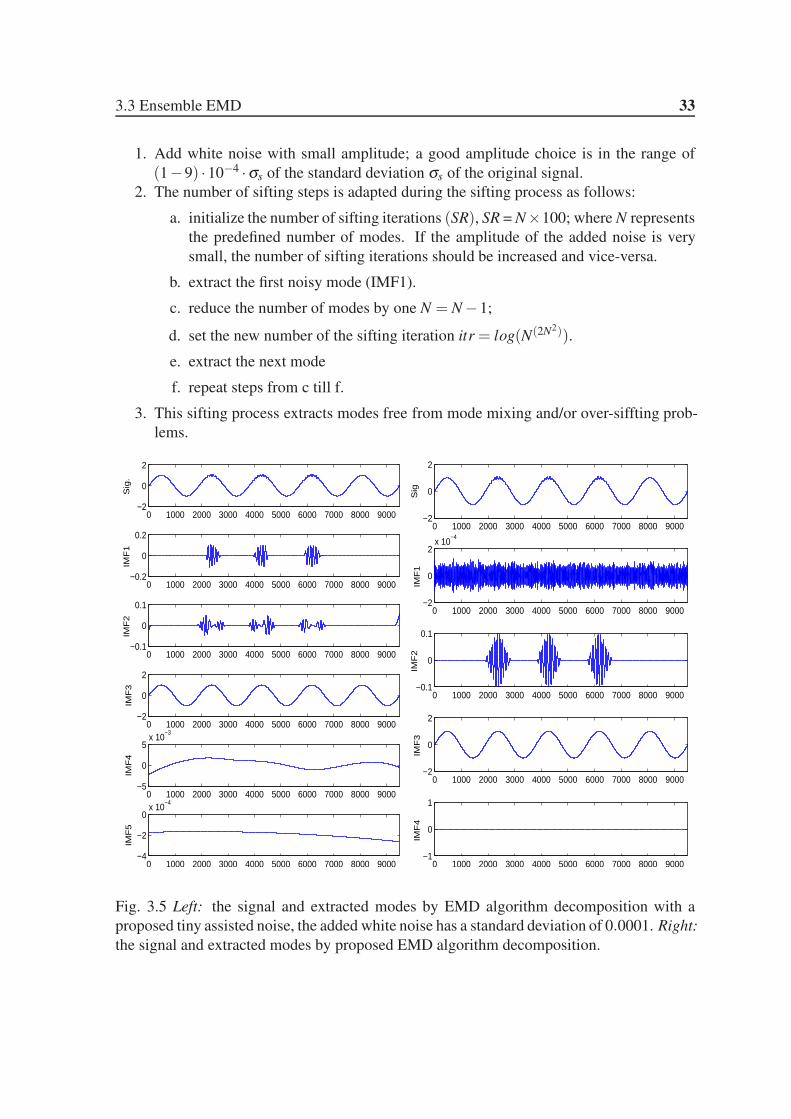
3.3 Ensemble EMD 33
1. Add white noise with small amplitude; a good amplitude choice is in the range of
(1−9) ·10−4 ·σs of the standard deviation σs of the original signal.
2. The number of sifting steps is adapted during the sifting process as follows:
a. initialize the number of sifting iterations (SR), SR = N×100; where N represents
the predefined number of modes. If the amplitude of the added noise is very
small, the number of sifting iterations should be increased and vice-versa.
b. extract the first noisy mode (IMF1).
c. reduce the number of modes by one N = N−1;
d. set the new number of the sifting iteration itr = log(N(2N2)).
e. extract the next mode
f. repeat steps from c till f.
3. This sifting process extracts modes free from mode mixing and/or over-siffting prob-
lems.
0 1000 2000 3000 4000 5000 6000 7000 8000 9000−2
0
2
Sig
.
0 1000 2000 3000 4000 5000 6000 7000 8000 9000−0.2
0
0.2
IMF
1
0 1000 2000 3000 4000 5000 6000 7000 8000 9000−0.1
0
0.1
IMF
2
0 1000 2000 3000 4000 5000 6000 7000 8000 9000−2
0
2
IMF
3
0 1000 2000 3000 4000 5000 6000 7000 8000 9000−5
0
5x 10
−3
IMF
4
0 1000 2000 3000 4000 5000 6000 7000 8000 9000−4
−2
0x 10
−4
IMF
5
0 1000 2000 3000 4000 5000 6000 7000 8000 9000−2
0
2
Sig
0 1000 2000 3000 4000 5000 6000 7000 8000 9000−2
0
2x 10
−4
IMF
1
0 1000 2000 3000 4000 5000 6000 7000 8000 9000−0.1
0
0.1
IMF
2
0 1000 2000 3000 4000 5000 6000 7000 8000 9000−2
0
2
IMF
3
0 1000 2000 3000 4000 5000 6000 7000 8000 9000−1
0
1
IMF
4
Fig. 3.5 Left: the signal and extracted modes by EMD algorithm decomposition with a
proposed tiny assisted noise, the added white noise has a standard deviation of 0.0001. Right:
the signal and extracted modes by proposed EMD algorithm decomposition.

3.4 Bi-dimensional Ensemble Empirical Mode Decomposition 34
Hence, according to the proposed solution and after the original signal has been decom-
posed, see Fig. 3.5, following notices were observed: when white noise with a small ampli-
tude is added without changing the number of sifting iterations (first step of the proposed
improvements), an EEMD succeeds to estimate the underlying modes rather correctly, but
it still fails to cope with the added noise. Also over-sifting appeared because the intermit-
tency remained in the components IMF1 and IMF2. While applying the proposed method,
see Fig. 3.5 (right), the modes obtained perfectly match the original ones: the added noise
in IMF1, the intermittent signal in IMF2 and the pure signal in IMF3. So the trade-off be-
tween the amplitude of the added noise and the sifting iterations is required. Hence a new
suggestion, to solve this kind of problem, is introduced. In addition to the performance of
this proposed improvement in coping such mode mixing problem, the computational load is
reduced compared to an EEMD-50 analysis roughly 6−fold.
3.4 Bi-dimensional Ensemble Empirical Mode Decomposi-
tion
Soon after its invention, EMD has been extended to higher dimensions [46, 109, 126–
128, 166] including complex-valued data sets [2, 93, 148]. Obviously, two-dimensional
image data sets were of special interest [130]. In a first approach, such two-dimensional
data was treated as a collection of one-dimensional slices, which were decomposed with
one-dimensional EMD. This procedure is called pseudo-two-dimensional EMD [166]. How-
ever, pseudo-2D-EMD needs a coherence structure associated with the spatial scales in a
particular direction, which significantly limits its use. These recent developments in analy-
sis methods for non-linear and non-stationary data sets have received considerable attention
by image analysts. Thus several attempts have been started lately to extend EMD to multi-
array data sets like two-dimensional (2D) data arrays and images. These extensions are
variously known as bi-dimensional EMD (BEMD), image EMD (IEMD), 2D EMD and so
on [38, 87, 90, 91, 109–111, 167, 168]. The most demanding operation of these algorithms
involves an envelope surface interpolation step. In [38] the influence of various interpola-
tion methods is studied, and a sifting process is proposed based on a Delaunay triangulation
with subsequent cubic interpolation on triangles. In [12, 13] the envelope surface interpo-
lation step is replaced by either a direct envelope surface estimation method or radial basis
function interpolators. In [173] a new two-dimensional EMD (2DEMD) method is pro-
posed, which is claimed being faster and better-performing than current 2DEMD methods.
In [167] rotation-invariant texture feature vectors are extracted at multiple scales or spatial
frequencies based on a BEMD. Also, in [109–111] the BEMD-based texture extraction al-
gorithm is demonstrated in experiments with both synthetic and natural images. Finally, the
modified 2D EMD algorithm proposed in [167] implements the FastRBF algorithm in an es-
timation of the envelope surfaces. Some of these works exploit decompositions to compute
texture information contained in the images. Textures are an especially relevant feature of
biomedical images if their subsequent classification is intended as is the goal of this thesis
also.

3.4 Bi-dimensional Ensemble Empirical Mode Decomposition 35
Besides a genuine 2D implementation of the BEMD process, 1D EMD has also been
applied to images to extract 2D IMFs or bi-dimensional IMFs (BIMFs) [91, 92]. The lat-
ter technique treats each either row or each column of the 2D data set separately by a 1D
EMD, which renders the sifting process faster than in a genuine 2D decomposition. But
this parallel 1D implementation results in poor BIMF components compared to the canon-
ical 2D procedure due to the fact that the former ignores the correlation among the rows
and/or columns of a 2D image [89]. A major breakthrough has been achieved by Wu et
al. [166], who recently proposed a Multi-dimensional Ensemble Empirical Mode Decom-
position (MEEMD) for multidimensional data arrays. The well-known ensemble empirical
mode decomposition (EEMD) is applied to slices of data in each and every dimension in-
volved. The combination of partial IMFs to the final multi-dimensional IMF is based on a
comparable-minimal-scale-combination principle (CMSC-principle). MEEMD turned out
to be very efficient in practical applications, especially if applied to the two-dimensional
case, and will be used in this thesis to analyze fMRI images taken while subjects were
performing a cognitive task.
Following the BEEMD approach developed by Wu et al. [166] as a canonical BEMD
variant and contrast it with a novel fast and stable bi-dimensional EMD (GiT-BEMD) ap-
proach, that replaces the cubic spline interpolation step by an interpolation with splines in
tension employing Green’s functions [160], are deeply considered. Although, cubic splines
are in widespread use because of their smooth shape, these functions can exhibit unwanted
oscillations between data points. Adding tension to the spline overcomes this drawback.
Here, a technique for interpolation and gridding in bi-dimension EMD applications, using
Green’s functions for splines under tension, is used as well as examining some of the proper-
ties of these functions. The technique is borrowed from geophysics where it is in use already
since more than a decade [159]. Physical sciences have a frequent need for data interpola-
tion and griding. Such tasks are commonly accomplished by averaging [157] and finite
difference methods [20] employing cubic splines on a regular grid. Introducing surface
tension often helps to suppress undesired oscillations of such splines [142]. The Generic
Mapping Tools offer a software package implementing an algorithm which uses continuous
curvature splines under tension [161, 162]. Minimum curvature gridding, based on Green’s
functions of the bi-harmonic operator, has been proposed first by [134]. It offered enhanced
flexibility by employing both data values and gradients to constrain the interpolating surface,
allowed least squares fitting to noisy data sets and could evaluate the surface at any location
instead of being confined to a regular grid. However, the appearance of extraneous inflection
points, common to all minimum curvature methods, still represented a major obstacle to ap-
plications. Wessel and Bercovici [160] generalized the approach of Sandwell by including
surface tension to the Green’s function expansion of the interpolating surface. In summary,
for moderate amounts of data, the Green’s function technique is superior to conventional
finite difference methods because both data values and directional gradients can be used to
constrain the model surface. Also, noise can be suppressed easily by striving a least-squares
fit rather than considering a strict interpolation, and the model can be estimated at arbitrary
locations rather than only on a rectangular grid [160]. Moreover, including surface tension
greatly improves the stability of the method relative to gridding without tension. Recently,

3.4 Bi-dimensional Ensemble Empirical Mode Decomposition 36
Wessel presented a Green’s function based general purpose interpolator for both Cartesian
and spherical surface data called Greenspline [159] (available at http:
www.soest.hawaii.edu/pwessel/greenspline).
In this thesis, joining the Green’s function method with the BEMD technique is pro-
posed, thus eliminating the poor interpolation effects and reducing the computation time
for each iteration. Most favorably, this interpolation technique only needs few iterations
for estimating each BIMF. The proposed Green’s function in tension BEMD (GiT-BEMD)
method thus can be a good alternative providing an efficient BEMD processing.
The organization of the rest of this chapter is as follows: Before introducing the novel
concepts of GiT-BEMD, the regular BEMD process is introduced. The detailed description
of the proposed GiT-BEMD algorithm is given, next. Then, the method of detecting local
extrema suggested in GiT-BEMD is explained to further understanding of the proposed
envelope estimation technique, since it requires information about local extrema as its basic
ingredients. The final section, describes the new method of envelope estimation. Further
simulation results with various images comparing GiT-BEMD and canonical BEEMD are
given also in chapter 7.
3.4.1 General BEMD
General BEMD is a sifting process that decomposes X(m,n) into multiple hierarchical com-
ponents known as BIMFs. Similar to 1D sifting process, a 2D can be summarized in the
following iterations:
1. Initialization: set S(m,n) = X(m,n) . Identify all local maxima and local minima of
S(m,n) .
2. Interpolate the local maxima (resp. minima) to obtain the surface upper envelope
emax(m,n) and local minima (resp. lower envelope emin(m,n)) to obtain surface lower
envelop.
3. The mean σ(m,n) = [emax(m,n) + emin(m,n)]/2 is computed and subtracted from
S(m,n) to obtain S′(m,n) = S(m,n)−σ(m,n) .
4. Update S(m,n) by S′(m,n). Repeat steps 1 to 3 until the stopping criterion is met.
3.4.2 Canonical BEEMD
The general BEMD sketched above has been adapted to deal with two-dimensional data ar-
rays, especially images. This canonical BEEMD will be described in detail in the following.

3.4 Bi-dimensional Ensemble Empirical Mode Decomposition 37
Analyzing 2D data arrays, for example an fMRI brain slice, one starts by applying EEMD
to each column X∗n ≡ xn of the M×N - dimensional data matrix X
X = [xm,n] =
x1,1 x1,2 · · · x1,N
x2,1 x2,2 · · · x2,N...
... · · · ...
xM,1 xM,2 · · · xM,N
(3.24)
The 1D-EEMD decomposition of the n-th column becomes
xn := X∗,n =J
∑j=1
C( j)∗,n =
J
∑j=1
c( j)1,n
c( j)2,n...
c( j)M,n
(3.25)
where the column vector C(J)∗,n represents the residuum of the n-th column vector of the
data matrix. This finally results in J component matrices, each one containing the j-th
component of every column xn,n = 1, . . . ,N of the data matrix X.
C( j) = [c( j)1 c
( j)2 · · · c
( j)N ] = [C
( j)∗,1 C
( j)∗,2 · · · C
( j)∗,N ]
=
c( j)1,1 c
( j)1,2 · · · c
( j)1,N
c( j)2,1 c
( j)2,2 · · · c
( j)2,N
...... · · · ...
c( j)M,1 c
( j)M,2 · · · c
( j)M,N
(3.26)
Next one applies an EEMD to each row of Eq. (3.26) yielding
C( j)m,∗ =
(
c( j)m,1c
( j)m,2 · · ·c
( j)m,N
)
=K
∑k=1
(
h( j,k)m,1 h
( j,k)m,2 · · ·h
( j,k)m,N
)
=K
∑k=1
H( j,k)m,∗ (3.27)

3.4 Bi-dimensional Ensemble Empirical Mode Decomposition 38
where c( j)m,n = ∑K
k=1 h( j,k)m,n represents the decomposition of the rows of matrix C( j). These
components h( j,k)m,n can be arranged into a matrix H( j,k) according to
H( j,k) =
h( j,k)1,1 h
( j,k)1,2 · · · h
( j,k)1,N
h( j,k)2,1 h
( j,k)2,2 · · · h
( j,k)2,N
...... · · · ...
h( j,k)M,1 h
( j,k)M,2 · · · h
( j,k)M,N
(3.28)
The resulting component matrices have to be summed to obtain
C( j) =K
∑k=1
H( j,k). (3.29)
Finally this yields the following decomposition of the original data matrix X
X =J
∑j=1
C( j) =J
∑j=1
K
∑k=1
H( j,k) (3.30)
where each element is given by
xm,n =J
∑j=1
K
∑k=1
h( j,k)m,n (3.31)
To yield meaningful results, components h( j,k)m,n with comparable scales, i. e. similar spa-
tial frequencies of their textures, should finally be combined [166]. Note, that the CMSC-
principle affords to have K = J. In practice, for two-dimensional data sets this implies
that the components of each row, which represent a common horizontal scale, and the com-
ponents of each column, which represent a common vertical scale, should be summed up
[166].
Hence, the CMSC - principle leads to BIMFs given by
S(k′) =K
∑k=1
H(k,k′)+J
∑j=k′+1
H(k′, j) (3.32)
which thus yields a decomposition of the original data matrix X into BIMFs according to
X =K
∑k′=1
S(k′) (3.33)
where S(K) represents the non-oscillating residuum. The extracted BIMFs can be considered
features of the data set which, according to the CMSC - principle, reveal local textures with
characteristic spatial frequencies which help to discriminate the functional images under
study.

3.4 Bi-dimensional Ensemble Empirical Mode Decomposition 39
Fig. 3.6 An illustration of the 2DEEMD decomposition of an fMRI image. IMFs along
each row or column represent textures of comparable scale and are to be summed up to
yield a BIMF. To improve visibility, histogram equalization has been applied on each image
separately.
Fig. 3.6 illustrates the 2DEEMD and the CMSC - principle in case of a decomposition
of an fMRI image. It clearly describes the steps of the 2DEEMD algorithm using an fMRI

3.5 A Green’s function-based BEMD 40
image, i. e. a single brain slice, as an example. The image presented in the upper left corner
represents the original fMRI image. The first column on the left side, with the exception of
the original image in the upper left corner and the reconstructed image represented on the
bottom left side, represents the component images resulting from decompositions along the
x-direction. The columns 2→ 6, except the last row, represent the component images result-
ing from a decomposition along the y-direction of each component image which resulted
from a decomposition along the x-dimension. The last row, except the reconstructed image
on the bottom left side, represents the final BIMFs of the original fMRI image obtained by
applying the CMSC - principle. Thus, canonical BEEMD is applied to the fMRI images
considered in this thesis.
3.5 A Green’s function-based BEMD
With the intention of overcoming the difficulty in implementing BEMD via the application
of surface interpolation, a novel approach of BEMD is proposed here based on a represen-
tation of upper and lower surface envelopes via suitable Green’s functions for spline inter-
polation including surface tension, so-called (GiT-BEMD). Introducing a tension parameter
alleviates surface interpolation problems and greatly improves the stability of the method
relative to gridding without tension. Based on the properties of the new proposed approach,
GiT-BEMD is considered a fast and stable technique for image decomposition. GiT-BEMD
thus differs from the canonical BEEMD algorithm basically in the process of robustly esti-
mating the upper and lower envelope surfaces, and in limiting the number of iterations per
BIMF to a few iterations only. Hence, the GiT-BEMD is considered an algorithm of supe-
rior efficiency compared to other BEMD algorithms. The details of the extrema detection
and surface formation of the GiT-BEMD process are discussed in the following section.
3.5.1 Extraction of local extrema
Local extrema are points that have the largest or smallest pixel values relative to their K-
connected neighbors, therefore in a 2D image the pixel with coordinates (x,y) has 8 con-
nected neighbors with coordinates (x±1,y),(x,y±1),(x±1,y±1),(x±1,y∓1). The 2D
region of local maxima is called a maxima map, and the 2D array of local minima is called
a minima map, respectively. Like some BEMD variants, a neighboring window method
is employed to detect local extrema during intermediate steps of the sifting process for es-
timating a BIMF of any source image. Here, a data point/pixel is considered as a local
maximum (minimum), if its value is strictly higher (lower) than all of its neighbors. Let
P = {Pi|i = 1, ....N} be a set of local minima (maxima) of an x×y- dimensional data matrix
such that it exists a small (large) neighborhood around any such locally optimal point Pi on
which the pixel value is never larger (smaller) than f (xi,yi) at Pi. Local extrema occur only
at critical points. Let S(x,y) = fxx fyy− ( fxy)2 measure the curvature of the surface. If S > 0
at a critical point, then the critical point Pi is a local extremum. The signs of fxx and fyy
determine whether the point is a maximum or a minimum. If S ≤ 0 at a critical point, then

3.5 A Green’s function-based BEMD 41
the point Pi is a saddle point. In practice, a 3×3 window results in an optimal extrema map
for a given 2D image for many applications.
3.5.2 Green’s function for estimating envelopes
In BEMD, spline interpolation is basically used to find the smoothest surface passing through
a grid of irregularly spaced extrema, either maxima or minima. In this work it is proposed to
employ Green’s functions, deduced from proper data constraints, to expand the interpolating
surface under tension. Thus the envelope surfaces connecting local extrema in 2D space are
determined to minimize the curvature of the surface in the presence of surface tension [160].
Interpolation with Green’s functions implies that the points of the interpolating envelope
surface can be expressed as
s(xu) =N
∑n=1
wnΦ(xu,xn) (3.34)
where xu denotes any point where the surface is unknown, xn represents the n-th data con-
straint, Φ(xu,xn) is the Green’s function and wn is the respective weight in the envelope
representation. Several works discuss the use of Green’s functions in interpolation prob-
lems (see for example [159]). Following the basics of the Green’s function method for
spline interpolation using surface tension are summarized.
It has been shown by Sandwell [134] that the Green’s function Φ(x) obeys the following
relation at any data constraint xn, n = 1, . . . ,N
[
D∆2op−T ∆op
]
Φ(xu,xn) = δ (xu−xn) (3.35)
where, ∆2op and ∆op = ∇2, denote the bi-harmonic, the Laplace and the Nabla operator,
respectively, D is the flexural rigidity of the curve or surface, T is the tension used at the
boundaries, and Φ(xu,xn) represents the Green’s function containing the spatial position
vectors xu,xn as argument. With vanishing surface-tension, i. e. T → 0, the minimum
curvature solution Φ(xu,xn) = x2 log(x), x = |xu− xn| is achieved [134]; while in case of
a vanishing surface rigidity, i. e. D→ 0, the solution approaches Φ(xu,xn) = log(x). The
general solution is expected to retain these limiting characteristics. To obtain the former,
rewrite Eq. (3.35) in terms of the curvature Ψ(x) = ∇2Φ(x) of the Green’ s function and
transform it to the conjugate Fourier domain where it then reads
[
∆op +p2
k2
]
Ψ(k) =− 1
T
p2
k2. (3.36)
Here k = |k| represents the radial wavenumber, p2 = TD
, k denotes the wavenumber vector
and Ψ(k) represents the Fourier transform of Ψ(x). In Fourier space, the solution is obtained
as
Ψ(k) =− 1
T
( p2
k2 + p2
)
(3.37)

3.5 A Green’s function-based BEMD 42
From this the general solution of Eq. (3.35) in a 2-D spacial domain [160] can be
achieved by using the inverse Hankel transform as
Ψ(x) =− 1
T
∫ ∞
0
p2
k2 + p2J0(kx)kdk =− 1
Tp2K0(px) (3.38)
where K0 denotes the modified Bessel function of the second kind and order zero given
by
K0(px) =
∫ ∞
0
cos(kpx)dk√
k2 + p2∝
{
exp(−px) if px→ ∞− log(px) if px→ 0
(3.39)
Integrating Ψ(x) twice and rescaling, finally, yields the Green’s function Φ(x) and its
local gradient ∇Φ(x) as
Φ(xu,xn) = log(p|xu,xn|)+K0(p|x,xn|) = log(pxun)+K0(pxun) (3.40)
∇Φ(xu,xn) =
[
1
pxun−K1(pxun)
]
p(xu−xn)
|xu−xn|(3.41)
where p ∝ T represents the tension parameter, |.| denotes the Euclidean distance and K0(.)represents the modified Bessel function. Hence, by decreasing the tension parameter p ∝ T ,
the solution is expected to reach the minimum curvature solution represented by the bi-
harmonic Green’s function [134]. In contrary, increasing the tension parameter T , thus also
p, renders the arguments of Φ(x) large and leads to an interpolating surface dominated by
tension. Thus varying the tension p achieves a continuous spectrum of Green’s functions
reflecting the trade-off between the minimum curvature solution driven by the log(px) term
and the impact of the surface tension via the modified Bessel function K0(px). Thus, Includ-
ing N data constraints yields for the defining equation and its solution [134]
∆op
[
∆op− p2]
c(xu) =N
∑n=1
wnδ (xu−xn)
c(xu) =N
∑n=1
wnΦ(xu−xn) (3.42)
The coefficients wn can be obtained by solving the system of linear equations Gw = c
where the Green’s matrix collects all Green’s functions Φ(xm− xn) at the data constraints
m,n = 1, . . . ,N. Corresponding slopes sm in directions nm can be obtained by evaluating the
relations
sm =N
∑m=1
wm∇Φ(xm−xn) · n)m m = 1, . . . ,N.

3.5 A Green’s function-based BEMD 43
In summary, the interpolation procedure is based on two steps: the first step estimates
the weights w = [w1 w2 . . .wP] and the second step estimates the interpolating envelope
surface:
• The surface values s(xn) = [s(x1, . . . ,s(xN]T ≡ c = [c1,c2, . . . ,cN ]
T are known in a
total of N locations xn = [xn,yn]T , then using the interpolation Eq. (3.34) for each of
the known points a linear system with N equations is obtained
Gw = c
where n-th row of matrix G is the evaluation of the Green’s function Φ(xn,xm),m =1,2 . . .N. Therefore solving for the weights w = G−1c.
• Using the weights w, the value s(xu)≡ cu of the envelope surface can be estimated at
any point xu by solving Eq. (3.34), which can be re-written as
cu = wT Φ (3.43)
where the vector Φ = [Φ(xu,x1) Φ(xu,x2) . . .Φ(xu,xN)]T contains the Green’s func-
tion values of all distances between the N data constraints and the considered location.


Chapter 4
Features Extraction
A contour detecting system consists of a series of stages, of which the texture extraction,
feature extraction and classification are the most crucial for its overall performance. The
feature extraction reduces the dimensionality of the sample space of the extracted textures
by extracting the most discriminatory information. The feature extraction step may also al-
leviate the worst effects of the so-called ’curse of dimensionality’. Hence, the performance
of the feature extraction stage has a significant impact on the performance of the next stages,
feature selection and classification. If the most informative set of features is selected, the
workload of subsequent classifiers will be low. On the contrary, if the features with little dis-
criminatory power are selected, an even more sophisticated classification model may not be
able to achieve the goal. But, of course, some additional issues should be considered even
having selected the best features, for example parameter selection to enhance the classifica-
tion performance. However, feature extraction is still a challenge and widely dependent on
the characteristics of the dataset. For example, in pattern recognition tasks, a good feature
extractor with high-dimensional sample spaces might not work well in situations where the
dimensionality of the sample space is small.
Three powerful feature extraction techniques for high-dimensional spaces like fMRI
data like Principle and Independent Component Analysis (PCA and ICA) and Non-negative
Matrix Factorization (NMF), are used in this study. High-dimensional spaces are quite
different from the three-dimensional (3-D) space in terms of geometrical and statistical
properties. For example, the volume of an fMRI dataset and corresponding Volume In-
trinsic Mode Functions (VIMFs) extracted by BEMD/GiT BEMD are considered as 3-D
space in terms of geometrical properties and for visualization purposes, but it belongs to a
high-dimensional space when this volume is considered an input vector to a classifier. Al-
though high-dimensional sample spaces contain more information concerning the capability
of distinguishing different sample class with better accuracy, classifiers that carry out com-
putations at full dimensionality may not take advantage of high-dimensional sample spaces
if there are insufficient training samples. Hence, reliable density estimation is extremely im-
portant but complicated. Therefore, the dimensionality of the sample space must be reduced
via dimension reduction and feature extraction methods before the application of a classifier
to data samples in high-dimensional spaces can be considered. Thus, in order to retain the
most informative and discriminatory information which the high-dimensional sample spaces

4.1 Principal Component Analysis 45
provide, powerful dimension reduction techniques are needed. The aim of feature extraction
is to reduce the high-dimension of fMRI data but at the same time retain as much as possible
of their discriminatory information. Hence, a good feature extractor selects features which
are similar for patterns in the same class and very different for patterns in different classes.
The feature extraction is quite important for fMRI image classification, because fMRI is in-
herently high-dimensional. Typically, one volume of fMRI contains about 160,000 voxels,
and one experiment will include several volumes. Processing all these voxels as features for
classification is practically impossible because of computer memory and computation time
limitations. It is necessary to consider some projections, or use only part of these voxels
(down-sampling), to reduce the dimensionality of fMRI data. After the feature extraction,
feature selection can be performed. Since the dimensionality of the sample space is reduced
after the feature extraction step, extraction will yield savings in memory and time consump-
tion. The object of feature selection is to use part of these extracted features as input of a
classifier. In many cases, even after feature extraction has been performed, the number of
features is still too large to feed the classifier or they contain artifacts. Feature selection is
thus required to filter our extracted features and identify the group of most discriminatory
features which can achieve the best classification performance.
In this thesis, PCA, ICA and NMF feature extraction methods, which exploit the advan-
tages of high-dimensional spaces, are proposed. Beside such techniques reduce the high-
dimensional of our images, the key point of choosing these techniques as feature extraction
methods is their speed as well.Then, a variation of a linear subspace classifiers which is
suitable for detecting contour tasks in high-dimensional spaces is applied. These classifiers
were also generalized to the nonlinear case by employing kernel functions. The useful-
ness of the proposed methods are demonstrated with experiments using our dataset. Con-
sequently, it can help to improve the performance of classification rate. Also, the effect of
these feature selection techniques, which are used in this thesis, will be discussed in detail
later on.
4.1 Principal Component Analysis
Principal Components Analysis (PCA) is a rather general statistical procedure used in many
applications, such as statistical data analysis, feature extraction and data compression. The
goal of PCA is to find a smaller informative set of variables with less redundancy which
represent the original signal as accurately as possible [62]. In PCA, the redundancy is mea-
sured in terms of correlation between the observed data. This will be further strengthened
in the next section, where ICA is introduced. In this chapter, the theoretical details of PCA
are explained.
Problems arise when one wish to perform classification and recognition in a high-dimensional
space. The aim of PCA is to decrease the dimensionality of the data by retaining as much
as possible of the total data variance of our original data set.
On the other hand, dimensionality reduction implies some information would be lost.
Hence, the best low-dimensional space is determined by the best principal components as
its coordinate axes. The main advantage of PCA, in this thesis, is using it to reduce the size

4.1 Principal Component Analysis 46
of our dataset for detecting textures and their contours. The extracted textures from the past
step, see chapter 3, are stored in the form of feature vectors in the database. These feature
vectors are determined by projecting each and every trained volume to the set of eigenvol-
umes obtained. PCA serves to determine these eigenvolumes with which the dimensionality
of a large data set may be reduced then.
4.1.1 Eigenvalues and Eigenvectors
The eigenvectors of a linear operator are non-zero vectors, which result in a scalar multiple
of them upon action of the operator on them. This scalar is then called eigenvalue (λ )associated with the eigenvector (z). An eigenvector is thus a vector that is simply scaled
by a linear transformation. Such simple scaling can be effected by the action of a matrix
operator, for example. When a matrix acts on a vector, only the magnitude of the vector is
changed not its direction.
Az = λz (4.1)
where A is a matrix operator. Hence,
(A−λ I)z = 0 (4.2)
where I is the identity matrix. This is a homogeneous system of equations. And it is known,
from fundamental linear algebra, that a non-trivial solution exists if and only if the charac-
teristic equation is obeyed:
det(A−λ I) = 0 (4.3)
where det denotes the determinant. When evaluated, the solution becomes a polynomial
of degree n. This is called characteristic polynomial of A. If A is n× n, then there are
n solutions or n roots of the characteristic polynomial. Thus there are n eigenvalues of A
satisfying the following equation:
Azi = λizi (4.4)
where i = 1,2,3, .....n. If the Eigenvalues are all distinct, there are n associated linearly
independent eigenvectors, whose directions are unique and which span an n dimensional
Euclidean space.

4.1 Principal Component Analysis 47
4.1.2 Eigendecomposition of VIMFs
Dimension reduction can be achieved by applying a Principal Component Analysis (PCA).
To perform a PCA, VIMFs from all Ns j = 19 subjects and for the two conditions, CT and
NCT, are collected into a data matrix M
M =
m11 . . . m1S
m21 . . . m2S...
. . ....
mR1 . . . mRS
(4.5)
Then VIMFs can be projected onto eigenvolumes resulting from a PCA, and the result-
ing projections are used as appropriate features for classification. The goal of a principal
component decomposition of the VIMFs, obtained through a 2DEEMD and/or GiT-BEMD,
is to compute the eigenvolumes U of the co-variance or, for centered data (see Fig. 4.1),
correlation matrix R that span the space of all voxels. This allows for a new representation
of the data in an orthogonal axis system which maximizes the variance of the data along
each principal direction. Projecting all VIMFs onto these eigenvector directions reveals the
contribution of each eigenvector to the volume mode. PCA eigenvolumes can be determined
by decomposing the R×S dimensional matrix M of VIMFs with the help of a singular value
decomposition (SVD), see Fig. 4.1.
M = UDVT (4.6)
Fig. 4.1 Graphical representation of SVD.
where, D denotes a diagonal matrix (i. e. a square matrix with non-zero entries only along
the diagonal), which contains derived constants called singular values sorted in descending
order. Each singular value represents the amount of variance that is captured by a particular
dimension. The left-singular and right-singular vector linked to the highest singular value
represent the most important dimension in the data (i.e. the dimension that explains the most
variance of the matrix); the singular vectors linked to the second highest value represent the
second most important dimension (orthogonal to the first one), and so on. Furthermore, U

4.1 Principal Component Analysis 48
and V are the eigenvector matrices of the non-normalized correlation matrix R = MMT
and the related kernel matrix K = MT M, whose corresponding column vectors u,v form
orthogonal eigenvectors in spaces of dimension R×R and S×S, respectively. A key property
of the derived vectors is that all directions are orthogonal (i.e. linearly independent) to each
other, so that each eigenvector is uncorrelated to the others. Very briefly, PCA or SVD thus
performs a second order decorrelation of a dataset.
Intuitively, SVD is able to transform the original matrix with an abundance of overlap-
ping dimensions into a new, many times smaller matrix that is able to describe the data in
terms of its principal components. Due to this dimension reduction, a more succinct and
more general representation of the data is obtained. Redundancy is filtered out, and data
sparseness is reduced. Therefore the columns of U span the voxel space while the columns
of V span the (participants× conditions) space. It is important to note that from only S≪ R
observations the components of the eigenvector matrix U cannot be determined reliably.
However, one has to resort to study the related kernel matrix as only an eigenvalue decom-
position of matrix K is feasible. This finally yields, substituting results from above, for the
singular value decomposition of the matrix of observations M the following relation
K = MT M = (UDVT )T UDVT = (VDUT )UDVT
= VD2VT = VΛVT (4.7)
Therefore the eigenvalues λs are the square of the singular values ds and the eigenvector
matrix V is the right eigenvector matrix of SVD. Hence, Λ = D2 and the eigenvector matrix
U of the correlation matrix R can be obtained from the matrix of observations M and its
SVD via U = MVΛ−1/2.
Now consider projecting all data vectors onto the new basis vectors, i. e. consider the
projections Z := UT M. Hence Z represents the matrix of projections of the data vectors M
onto the eigenvectors U of the correlation matrix R which also span the space of all voxels
of the component images. From the discussion above it follows that
UT M := Z = DVT = Λ1/2VT (4.8)
Note that both, D and V follow from an eigendecomposition of the kernel matrix of
the observations. Every row Zn,∗ of the projection matrix Z contains a projection of a data
vector onto one of the new basis vectors U∗,n. The latter are ordered via their corresponding
eigenvalues ds =√
λs. This allows to select only the most informative projections to be used
as features for a classifier, for example. Anyway, only S≪ R projections can be obtained
which renders the problem tractable.
In summary, the eigenvalue decomposition of the kernel matrix K, i. e. the matrix
of inner products of the data vectors, provides all ingredients to compute the projections
onto at most S directions. Each row of Z contains a projection onto one such basis vector.
Again note that the latter are ordered via their corresponding eigenvalues λs. Considering
the data set studied, a further dimension reduction is possible by selecting a subset of those
S projections, e.g. choosing the L < S leading rows of the projection matrix Z. Then the

4.2 Independent Component Analysis 49
classifier will only have L ≤ S inputs and S examples which represents a stable situation
in the sense that sufficient information is provided to the classifier to achieve a reliable
classification of the data. Note that this decomposition into eigenvolumes has been applied
to both the average volumes ∠Vsc(x,y,z)〉 as well as to the VIMFs resulting from a preceding
BEEMD/GiT-BEMDdecomposition.
4.2 Independent Component Analysis
Independent component analysis (ICA) aims to find a linear representation of data based on
maximally non-Gassian components which renders them statistically independent.
Independent components are achieved by applying a, yet to be determined, S×S rotation
matrix W to the projected data Z. The INFOMAX algorithm [34] was used to estimate the
rotation matrix, and the new representation of the projected data is obtained via
S = WZ = WUT M (4.9)
Afterwards the rows of S are re-ordered according to their correlations to the rows of
Z as the obtained independent components lack any natural ordering. Therefore after re-
ordering, the first row of S should have the largest correlation with the first row of Z, the
second row of S should have the largest correlation with the second row of Z and so on.
This allows to select only the most informative projections to be used as features for
a classifier. Anyway, only S≪ R projections can be obtained which renders the problem
tractable.
In contrary to PCA, the ICA spatial components (patterns) have to be not only decor-
related (orthogonal), but statistically independent with few large voxel values in each com-
ponent. In Independent Component Analysis (ICA), the assumption is that of statistical
independence of the extracted sources, the so-called independent components. Statistical
independence is a much stronger requirement than decorrelation discussed in the last sec-
tion. In fact, all ICA algorithms employ decorrelation and centering, called whitening, as
the first step to independence. It can be shown that, assuming independence, one might
achieve a unique solution of the matrix decomposition, if at most one of the sources has a
Gaussian distribution and the mixing matrix has full column rank. The latter implies that
the number of mixtures is at least as large as the number of sources. Uniqueness in this
context means unique modulo scaling and permutation; performing these operations on S
can always be compensated by corresponding operations on the columns of W. In practice,
it is not straightforward to measure statistical independence, which therefore has to be ap-
proximated. To this end, a common approach is non-gaussianity [62]. From a hand-waving
interpretation of the central limit theorem it follows that any weighted sum of independent
sources is more “Gaussian" than the sources themselves. So maximizing non-gaussianity is
a way to reveal the underlying sources. This property can be quantified by the fourth-order
cumulant, called the kurtosis. The kurtosis K(x) := E(x4)− 3(E(x2)2) is measure for the
peakedness of a probability distribution p(x) and vanishes for a Gaussian. An alternative
measure is the negentropy, which is based on the information-theoretic concept of entropy.

4.3 Non-Negative Matrix Factorization 50
The entropy of a random variable is related to the information that its observation gives. The
more random, i.e., unpredictable and unstructured the variable is, the larger its entropy. Its
largest value among all random variable distributions of equal variance is found for a Gaus-
sian. Robust approximations of negentropy instead of kurtosis may enhance the statistical
properties of the resulting estimator. Examples of common ICA implementations are the
JADE algorithm [25], the INFOMAX algorithm [11] and the f astICA algorithm [61] .
Fig. 4.2 Top: Illustration example of 3-D data distribution and corresponding PC and IC
axes. Each axis is a column of the mixing matrix found either by PCA or ICA. Note that
axes of PCs are orthogonal while the IC axes are not. If only two components are allowed,
ICA chooses a different subspace than PCA. Bottom Left: Distribution of the first PCA
coordinates of the data. Bottom Right: Distribution of the first ICA coordinates of the
data. Note that since the ICA axes are nonorthogonal, relative distances between points are
different in PCA than in ICA, as are the angles between points (adapted from [94]).
4.3 Non-Negative Matrix Factorization
Non-negative Matrix Factorization (NMF) is another method to render the high-dimension
problem tractable. Non-negative matrix factorization is a data decomposition, data cluster-
ing and dimensionality reduction technique that has been becoming popular in various fields
such as image recognition, speech recognition and machine learning. The main idea behind

4.3 Non-Negative Matrix Factorization 51
NMF is to impose a non-negativity constraint on the factorization of the data matrix. This
constraint conducts a parts-based representation, because only additive and no subtractive
combinations are allowed. In many cases, this constraint is very useful for the inductive ca-
pabilities of the dimensionality reduction. The NMF algorithm can extract clear and distinct
characteristics from the studied data. The difference between the parts-based induction of
NMF and the holistic induction of global methods such as PCA (and the related singular
value decomposition) are illustrated in detail with an example from facial image recognition
in [79]. Lee and Seung [79] found there are a small number of prototypical faces represented
by the eigenvectors that are found by applying PCA to a database of facial images. Positive
as well as negative values could be associated with the produced eigenfaces. The point in
such methods that they are holistic: an eigenface contains all sorts of facial traits, and thus
represents a prototypical face. By taking a linear combination of various ’eigenfaces’, a
particular pattern of a face may be reconstructed. The way NMF results look like is quite
different. Instead of finding holistic, prototypical faces, the algorithm produces particular
facial traits (different kinds of eyes, noses, mouths and so on ). By enforcing a non-negative
constraint, the algorithm can make up a parts-based representation of facial images. A par-
ticular instance of a face may then be reconstructed by taking a linear combination of the
different parts. The very same characteristic will also prove to be beneficial for making
up projected representations from fMRI images. Recently, NMF has gained attention in a
variety of applications. So, non-negative matrix factorization (NMF) [79] is the name for a
group of algorithms in which a matrix M is factorized into two other nonnegative matrices,
H and W. Fig. 4.3 shows a graphical representation of non-negative matrix factorization.
M ≈ HW (4.10)
Fig. 4.3 A graphical representation of non-negative matrix factorization.
Typically the inner dimension k is much smaller than R,S so that both instances and
features are expressed in terms of a few components. As mentioned above, non-negative
matrix factorization enforces the constraint that all factor matrices must be non-negative, so
all elements must be greater than or equal to zero. This factorization may not always be
achieved perfectly, whence it can only be an approximate decomposition into non-negative
causes with non-negative weights. Obviously, the inner dimension has to be reduced, oth-

4.3 Non-Negative Matrix Factorization 52
erwise the factorization is completely arbitrary. Also, this decomposition is far from being
unique and needs to be regularized by additional constraints like minimum volume require-
ments. There are two objective functions that may be used in order to quantify the quality
of the approximation of the original matrix. One objective function minimizes the sum of
squares:
min ‖M−HW ‖F = min∑i
∑j
(
Mi j−∑k
HikWk j
)2
(4.11)
which is related to Gaussian error statistics. The other one minimizes the Kullback-Leibler
divergence following from Laplacian error statistics:
minDKL(M ‖HW) = min∑i
∑j
(
Mi j logMi j
(HW)i j
−Mi j +(HW )i j
)
(4.12)
Practically, the factorization can be efficiently carried out through the iterative applica-
tion of multiplicative update rules. The set of update rules that minimizes the Euclidean
distance are given in the following equations, Eq. (4.13) and Eq. (4.14).
Waµ ← Waµ(HT M)aµ
(HT HW)aµ(4.13)
Hia ← Hia(MWT )ia
(HWWT )ia
(4.14)
The set of update rules that minimizes the Kullback-Leibler divergence are given in Eq.
(4.15) and Eq. (4.16)
Waµ ← Waµ
∑i HiaMiµ
(HWiµ )
∑k Hka
(4.15)
Hia ← Hia
∑µ WaµMiµ
(HWiµ )
∑v Wav(4.16)
Matrices H and W are randomly initialized, and the update rules are iteratively applied
alternating between them. In each iteration, the matrices H and W are suitably normalized,
so that the rows of the matrices sum to one. The algorithm stops after a fixed number of itera-
tions, or according to some stopping criterion, for example when the change of the objective

4.3 Non-Negative Matrix Factorization 53
function drops below a certain threshold. The update rules are guaranteed to converge to a
local optimum. In practice, it is usually sufficient to run the NMF algorithm repeatedly in
order to find the global optimum. Note that fMRI images are non-negative but the extracted
modes are combining of negative and positive components (oscillations) because of nature
of the BEMD decomposition. So, in this work, the extracted modes are normalized between
0 and 1 before employing NMF.


Chapter 5
Classification
Functional magnetic resonance imaging (fMRI) is an neuroimaging technology which is
mainly used to detect brain activity distributions by measuring neuronal activity in the brain
during a specific task. Classification of fMRI scans using machine learning (ML) is a field
of interest in cognitive neuroscience and the medical community because of its potential
to provide an automated system of detecting neurological conditions while jointly giving
insight into potential causes of underlying disorders.
Discrimination has been successfully performed using spatially localized signal differ-
ences to distinguish among different groups (see for example [47, 174]). But it is also pos-
sible to make use of pattern recognition techniques to predict the stimuli being presented
from the corresponding brain images and activation patterns. One of the primary objec-
tive of this dissertation is the use of well-known classification methods in the context of an
event-related functional contour integration experiment where participants viewed images
of contour and non-contour stimuli, and test whether these classifiers can predict, depending
on the collected images, the cognitive state precisely from the stimulus response. The utility
of feature selection methods in improving the prediction accuracy of classifiers, trained on
functional neuroimaging data and corresponding extracted textures ( by canonical BEMD
and/or Git-BEMD), are explored in details. In addition, the optimization of classifiers’ pa-
rameters were considered to enhance their classification accuracy as well. To identify the
most informative textures, i.e. VIMFs, a support vector machine (SVM) as well as a random
forest (RF) classifier was trained for two different stimulus/response conditions. Classifica-
tion performance was used to estimate the discriminative power of the extracted VIMFs.
5.1 Support Vector Machine
A Support Vector Machine (SVM) is a classifier, which can deal with linear or nonlinear data.
The key concept of an SVM, which was first developed for binary classification problems,
is to define decision boundaries separating data points of different classes by a hyperplane.
The simplest approach of an SVM is the two class problem, which is initially done by con-
structing a hyperplane with maximum distance (margin) from these two classes. Thus, an
SVM classifier finds the optimal hyperplane maximizing the margin between positive and

5.1 Support Vector Machine 55
negative examples while jointly minimizing misclassification errors in the training set. SVM
classifiers generalize well and have been observed to outperform other classification meth-
ods in many practical applications. In some problems, however, the two classes are hard
to separate linearly. But an SVM can handle both simple, linear classification problems as
well as more complex, i.e. nonlinear classification problems. Both linearly separable and
non-separable problems are managed by an SVM. In case of complex, non-linearly separa-
ble problems, the SVM has the opportunity to transform the data with a mapping (or kernel)
function into a high dimensional space (feature space), where the decision hyperplane can
be constructed more easily. This principle is illustrated in Fig. 5.1
Fig. 5.1 Illustrates the principle of SVMs. left: illustrates the simple way of separating two
classes linearly . Right: illustrates how the data is hardly to separate non-linearly in two
dimensions. Hence one can use a kernel function to map the data into the feature space
(three dimensional in this example). In this feature space the data can be classified easily.
image adapted from http://www.imtech.res.in/raghava/rbpred/svm.jpg
5.1.1 Separating Hyperplanes
Consider a given training data set {zi,yi}Ni=1, in a dot product space Γ , with pattern vectors
z1, . . . ,zs ∈ Γ being the input vectors and yi ∈ {−1,1} the class labels. The seperating
hyperplane can be defined as
{z ∈ Γ < 〈w,z〉+b = 0},w ∈ Γ ,b ∈ R (5.1)
Where w is the vector orthogonal to the hyperplane and b is a bias related with the
distance of the hyperplane from the origin of the coordinate system. For a w with ‖ w ‖= 1
the term 〈w,z〉 is the length of z along the direction of w. In Eq. (5.1) one can multiply w
and b with the same non-zero constant. This undue freedom can be explained by using the
following definition(cf. [138]):
The pair (w,b) ∈ Γ ×R is called a canonical form of the hyperplane (Eq. (5.1)) with
respect to z1, . . . ,zs ∈ Γ , if it is scaled such that
mini=1,...,s
[〈w,zi〉+b = 1〉] , (5.2)

5.1 Support Vector Machine 56
which is to say that the point closest to the hyperplane in its canonical form has a distance
of 1‖w‖ , while
|b|‖w‖ is the perpendicular distance of the non-canonical hyperplane from the
origin. For any such separating hyperplane, uniquely characterized in its canonical form by
a pair (w,b), a classifier can be constructed as in Eq. (5.3). The different orientation leads
to two different, inverse to each other, decision functions (cf. [138]) :
fw,b : Γ →{±1}z 7−→ fw,b = sgn(〈w,z〉+b)
(5.3)
In case there is do not exist class labels, yi ∈ {±1}, which are associated with the zi,
the two hyperplanes cannot be distinguished. In case of a labeled dataset, the discrimina-
tion between classes can definitely be achieved: The two hyperplanes make opposite class
assignments. The goal is to find a solution fw,b, which correctly classifies the labeled exam-
ples (zi,yi) ∈ Γ ×{±1}. This solution should satisfy fw,b = yi for all i,see Fig. 5.2.
Fig. 5.2 Illustrates example of different separating hyperplanes. The thick line is the optimal
hyperplane in this example.
5.1.2 The Geometric Margine
For a hyperplane {z ∈ Γ |< 〈w,z〉+b = 0}, the expression
ρ(w,b)(z,y) := y(〈w,zi〉+b)
‖ w ‖ (5.4)
measures the margin of the point (z1,y1) ∈ Γ ×{±1} from the hyperplane. The mini-
mum value
ρ(w,b) := mini=1,...,s
ρ(w,b)(zi,yi) (5.5)

5.1 Support Vector Machine 57
is called the geometrical margin of (z1,y1), . . . ,(zs,ys).In this thesis, from now on the margin always refers to the geometrical margin.
If a point (z,y) was classified correctly, the margin equals the distance between z and
the hyperplane. For a hyperplane
(w,b) :=( w
‖ w ‖ ,b
‖ w ‖)
where ‖ w ‖= 1
(5.6)
one can compute the quantity
y(
〈w,z〉+ b)
. (5.7)
The expression 〈w,z〉 simply considers the length of z in direction perpendicular to the
hyperplane, the adding of b equals the distance to it. Multiplying the expression with the
label y ensures that the margin is positive for correctly classified points, and negative for
incorrect classified points. For canonical hyperplanes the margin is 1‖w‖ . Hence, a larger
margin means a good classifier and as a consequence, the classification accuracy improves.
5.1.3 Optimal Margin Hyperplane
To define what an optimal hyperplane is simply means maximizing its margins in way that
can be identified in a computationally efficient way. Solving the optimization problem by
computing the best hyperplane with a set of examples (z1,y1), . . . ,(zs,ys),zi ∈ Γ ,yi ∈ {±1}can be done by finding a decision function
fw,b(z) = sgn(〈w,z〉+b) (5.8)
satisfying fw,b(zi) = (yi)
If such a function exists, canonically implies
yi(〈zi,w〉+b)≥ 1. (5.9)
Constructing an optimally separating hyperplane can be achieved by solving the opti-
mization problem:
minimizew∈Γ ,b∈R
τ(w) =1
2‖ w ‖2 (5.10)
subject to yi(〈zi,w〉+b)≥ 1 for all i = 1, . . . ,S (5.11)
Eq. (5.11) is called the primal optimization problem. As it represents a constrained
optimization problem, it can be related within a Lagrange formalism to a dual problem

5.1 Support Vector Machine 58
which has the same solutions, but is easier to solve. At first, one has to start with the
Lagrangian(α)
L(w,b,α) =1
2‖ w ‖2 −
s
∑i=1
αi(yi(〈zi,w〉+b)−1) (5.12)
where the αi ≥ 0 represent Lagrange multipliers. The aim is to maximize L with respect to
αi and minimize L with respect to w and b. From this it follows that
∂
∂bL(w,b,α) =
∂
∂wL(w,b,α) = 0, (5.13)
which leads to
s
∑i=1
αiyi = 0 (5.14)
w =s
∑i=1
αiyizi. (5.15)
According to the Karush-Kuhn-Tucker conditions (cf. [138]), only the αi that are non-
zero at the saddle point fulfill the constraints 5.11. Hence, one can derive the following
condition:
αi[yi(〈zi,w〉+b)−1] = 0 (5.16)
The patterns zi for which αi ≥ 0 are called Support Vectors (SVs). All of the other
patterns of the training examples are irrelevant.
To derive the dual form of the optimization problem one has to insert Eq. (5.14) and Eq.
(5.15) into the Lagrangian in Eq. (5.12):
maximizeα∈Rm
W (α) =S
∑i=1
αi−1
2
S
∑i, j=1
αiα jyiy j〈z(i),z( j)〉 (5.17)
subject to αi ≥ 0, i = 1, . . . ,S (5.18)
andS
∑i=1
αiyi = 0. (5.19)
where 〈z(i),z( j)〉 represents the dot product between the training data. The resulting decision
function, considering a test vector ztest to be classified, takes the form
f (ztest) = sgn
(
S
∑i=1
αiyi〈ztest ,z(i)〉+b
)
(5.20)

5.1 Support Vector Machine 59
5.1.4 Non-linear Support Vector Classifiers
In the previous section, only the linearly separable case was discussed. But what if the
data cannot be separated with a large margin hyperplane, rather would need a hypersurface?
Then, the formulation given above can be further extended to build a non-linear SVM. For
this extension, one can non-linearly transform the input data z1, . . . ,zS ∈ X into a high di-
mensional feature space using a mapping Φ : zi 7−→ zi. Such a transformation of the input
data enables a linear separation in the high-dimensional feature space, thus rendering the
classification of nonlinearly separable data possible. Applying such a mapping within a
SVM algorithm requires only simple modifications. Maximizing the corresponding target
function Eq. (5.17) and evaluating the related decision function Eq. (5.20) requires the
computation of dot products 〈Φ(z),Φ(zi)〉 in a high-dimensional feature space. The main
drawback of this approach is that it is computationally very expansive. Schölkopf et al.
[138] could show that one can use positive definite kernels to reduce these costs, i.e.:
〈Φ(z),Φ(zi)〉= k(z,zi) (5.21)
This kernel produces a decision function of the form
f (z) = sgn( S
∑i=1
yiαik(z,zi)+b)
(5.22)
The kernels used most often are the following:
• Linear kernel
k(z,zi) = zT zi,
• Polynomial kernels of degree d
k(z,zi) = 〈z,zi〉d ,
• Radial basis function (RBF)
k(z,zi) = exp(−‖z−zi‖2
σ2 ),
• Sigmoid kernels, so-called Multi-layer Perceptron (MLP)
k(z,zi) = tanh(γzT(i)z( j)+ r),
where k(., .) is positive definite for all σ values in the RBF kernel case, and with parameters
γ > 0,r < 0 in the MLP case. These parameters are user-defined and need to be assigned
before running the optimization algorithm. Due to the kernel trick, the optimization problem
turns into
maximizeα
W (α) =S
∑i=1
αi−1
2
S
∑i, j=1
αiα jyiy jk(zi,z j), (5.23)
subject to the constraints Eq. (5.18) and Eq. (5.19). Schölkopf et al. [138] show that for a
positive definite kernel k the matrix elements Qi j := (yiy jk(zi,z j)) is also positive definite. It

5.1 Support Vector Machine 60
turns out, that this is a convex problem which can be efficiently solved. The KKT conditions,
αi > 0 and Eq. (5.21) imply:
S
∑i=1
yiαik(z j,zi)+b = yi (5.24)
From this follows for the threshold b:
b = yi−S
∑i=1
yiαik(z j,zi) (5.25)
for all points with α j > 0 (Support Vectors).
The traditional SVM is solved using quadratic programming methods. However, these
methods are often computationally costly and are difficult to implement adaptively [36, 137].
Research has been undertaken to use a quadratic error criterion instead of the L1 norm used
for the SVM. Ridge regression methods, using a quadratic error criterion, were developed
for classification problems [36], and afterwards [96] used a quadratic error criterion to find
an iterative solution to their Lagrangian SVM networks. These methods still have inequality
constraints, however, recently Suykens et al. [146] proposed to modify the SVM method-
ology by introducing a least squares loss function and equality instead of inequality con-
straints, resulting in a so called Least Squares SVM (LS-SVM). Also recently a Sequential
Minimal Optimization SVM (SMO-SVM) was proposed by Platt [123] especially for non-
linear SVMs. Unlike QP-SVM and LS- SVM learning algorithms, which use numerical
quadratic programming (QP) as an inner loop, SMO uses an analytic QP step[123].
Accordingly, the common types of SVM methods QP-SVM, LS-SVM and SMO-SVM
are used in this thesis, to classify the binary contour integration problem in terms of de-
tecting a contour or non-contour condition from the stimulus response. Additionally, the
well-known kernels, listed above, are used as well.
5.1.5 Soft Margin Hyperplanes
So far, as it has been discussed in the previous two sections, generally SVMs can handle
linearly separable and nonlinearly separable input data depending on the following approach.
In real measurements noise is included always. Hence, a SVM algorithm must tolerate
noise and outliers, for instance a pattern which is mislabeled, which can crucially affect the
hyperplane, if it is constructed with one of the two methods discussed above.
To avoid this drawback, one has to use an algorithm which tolerates minor training errors.
According to this one needs so called slack variables ζ (cf. [138] )
ζ ≥ 0,where i = 1, . . . ,S (5.26)
to relax the separation constraints according to
yi(〈zi,w〉+b)≥ 1−ζi, i = 1, . . . ,S (5.27)

5.1 Support Vector Machine 61
Obviously, this constraint can always be fulfilled by making the ζi large enough. To
avoid any trivial solution, it is common to penalize large values in the objective function by
adding an additional term ∑i ζi. The simple case is the so called C-SVM with a constant
C > 0:
minimizew∈Γ ,ζ∈RS
τ(w,ζ ) =1
2‖ w ‖2 +
C
S
S
∑i=1
ζi (5.28)
subject to the constraints Eq. (5.26) and Eq. (5.27). In case the constraints are met
with ζi = 0, the corresponding point is no margin error. Otherwise, all points with ζ > 0
are margin errors and if ζi reaches too high values, a good separation cannot be always
guaranteed. According to [138], in the separable case the solutions have an extension
w =S
∑i=1
αiyizi. (5.29)
The coefficients αi are non-zero only for points (zi,yi) which meet precisely the con-
straint in Eq. (5.27). Hence, the αi can be computed by solving the quadratic optimization
problem:
maximizeα∈Rm
W (α) =S
∑i=1
αi−1
2
S
∑i, j=1
αiα jyiy jk(z(i),z( j)) (5.30)
subject to 0≤ αi ≤C
Sfor all i = 1, . . . ,S−1 (5.31)
andS
∑i=1
αiyi = 0. (5.32)
Due to Eq. (5.27), for all SVs z j for which ζ = 0, one can obtain the threshold like in Eq.
(5.24). So far, C has always been a constant, determining the trade-off between minimizing
the training error and maximizing the margin. Unfortunately, this parameter C is still a
rather unintuitive parameter and there is no a priori knowledge to select it. To avoid this,
C can be replaced by another parameter ν . The latter is explained in [138] as a parameter
which allows to control the number of margin errors and Support Vectors. The ν-SVC can
be written as:
minimizew∈Γ ,ζ∈RS,ρ,b∈R
τ(w,ζ ,ρ) =1
2‖ w ‖2−νρ +
1
S
S
∑i=1
ζi (5.33)
subject to yi(〈zi,w〉+b)≥ ρ−ζi (5.34)
and ζi ≥ 0, p≥ 0. (5.35)
where ρ in Eq. (5.35) is the margin of Eq. (5.4). Note that ν represents an upper bound
on the fraction of margin errors and a lower bound on the fraction of Support Vectors. Note

5.2 Random Forests 62
further that ν allows more errors, i.e. the margin increases. The quadratic optimization
problem for ν-SVC can be written as:
maximizeα∈Rm
W (α) =S
∑i=1
αi−1
2
S
∑i, j=1
αiα jyiy jk(z(i),z( j)) (5.36)
subject to0≤ αi ≤1
S(5.37)
S
∑i=1
αiyi = 0, (5.38)
S
∑i=1
αi ≥ ν (5.39)
Therefore, the resulting decision function can take the form
f (z) = sgn( S
∑i=1
αiyik(z,zi)+b)
(5.40)
5.2 Random Forests
A Random Forest (RF) is an ensemble classifier that consists of a collection of tree-structured
classifiers and outputs. It can be used for classification or regression by combining so-called
classification and regression trees (CARTs) (cf. [19]). CARTs are binary decision trees con-
structed by repeated splits of nodes into child-nodes. Nodes, which are not split any more
are called terminal nodes. This is illustrated in Fig. 5.4. The main idea which has to be
discussed is how to construct a CART and how to find the best split. For RF classifiers the
Gini criterion is used, (see section feature importance)
The RF combines Breiman’s "bagging" idea [19] and the random selection of features.
The growing of a CART begins with the root node, which contains the whole learning set.
Then, this set will be split into two subsets. The splitting point is called node. This process
continues until each node contains only one class (in this work CT or NCT ). Random
Forests use a large number of such CARTs, where each CART takes another bootstrap
sample from the training set. For every CART, the split variables are chosen randomly and
so every tree learns its own data set. The generalization error converges with the number of
trees. This makes it easy to decide how many trees should be used. The whole RF algorithm
is implemented as depicted in Fig. 5.3
5.2.1 Splitting Rule
The random forest algorithm, developed by Breiman [143], is a set of binary decision trees,
each performing a classification. The final decision is taken by majority voting. Each tree is
grown using a bootstrap sample from the original data set. Each node of the tree randomly

5.2 Random Forests 63
Fig. 5.3 Illustrates the flow chart of the random forest (RF) algorithm.

5.2 Random Forests 64
Fig. 5.4 An example of a classification tree. Here, brain is split into four smaller subsets
regions, resting state networks (RSNs)

5.2 Random Forests 65
selects a small subset of features for splitting the data into two subsets. An optimal split
separates the set of samples at each node into two supposedly more homogeneous or purer
sub-groups with respect to the class of its elements. The impurity level of each set of
samples with respect to class membership can be measured by the Gini index. Denoting
class labels by ωc, c = 1 . . .C, the Gini index of node i is defined as
G(i) = 1−C
∑c=1
(P(ωc))2 (5.41)
where P(ωc) is the probability of class ωc in the set of instances that belong to node i. Note
that G(i) = 0 whenever node i is pure, e.g, if its data set contains only instances of one class.
To perform a split, one feature zl is tested on the set of samples with n elements according to
zl > zth, which is then divided into two sub-groups (left and right) with nl and nr elements.
The change in impurity is computed as
△G(i) = G(i)−(nl
nG(il)+
nr
nG(ir)
)
(5.42)
That feature among all zl and the threshold zth which yields the largest decrease of the Gini
index is chosen to perform the split at node i. Each tree is grown independently, and no
pruning is applied on the grown trees. The main steps of this algorithm [63], are depicted in
the Fig. 5.3 and the following section.
5.2.2 Construction of a Tree
Constructing a tree requires a method to use the input data to determine the binary splits of
the training set into smaller subsets. The main goal is to find a split which produces subsets
purer than the parent sets. The construction of the tree contains three important steps:
1. Given a data set T with N examples, each with L features, select the number T of
trees, the dimension of the subset mtry< L of features, and the parameter that controls
the size of the tree (it can be the maximum depth of the tree, the minimum size of the
subset in a node to perform a split).
2. Construct the t = 1 . . .T trees.
(a) Create a training set Tt with N examples by sampling with replacement the orig-
inal data set. The out-of-bag data set Ot is formed with the remaining examples
of T not belonging to Tt .
(b) Perform the split of node i by testing one of the mtry = ⌊√
L⌋ randomly selected
features.
(c) Repeat step 2b up to the tree t is complete.
(d) Use the out-of-bag (OoB) data Ot as test set of the t-th tree. Keep track of the
votes for each class instance each time it is in the out-bag data set. The number
of false classifications, averaged over all cases, yields the OoB error estimate. In

5.2 Random Forests 66
this way an out-of-bag (OoB) error results, measuring the classification perfor-
mance of the RF classifier.
3. Repeat step 2 to grow the next tree if t 6= T . In this work T = 500 decision trees were
employed.
5.2.3 Out-of-Bag (OoB) Error Estimate
In Breiman’s implementation [17] of the RF, each tree is trained on about 66% of the avail-
able data set. As the forest is built, the rest of the data, about 33%, can be tested and reports
the misclassification rate. This process is called Out-of-Bag(OoB) error estimate. Accord-
ing to the nature of the calculation of the OoB error out of the training set, there is no need
for cross validation or additional testing. The OoB error estimation works by classifying
each instance left out in the construction with the RF. Then compare the classification re-
sults with the true assignments of the instances left out of the bag. Hence, the OoB error
is estimated by considering the proportion of times that the classification is not equal to the
true class averaged over all samples.
5.2.4 Feature Importance
The feature importance, which is well-known as variable importance, is a powerful tool
which was introduced by Breiman’s Random Forest [18]. It reports how importantly that
feature contributes in classifying the data. This is very helpful to make the classification
results easier interpretable. The commonly available variable importance measures are:
1. Mean Decrease Gini
The RF uses the Gini coefficient mentioned in Eq. (5.42) to determine how each fea-
ture contributes to split the nodes and leaves in the resulting RF. For two descendant
nodes, the Gini impurity criterion for each split made on a feature m is less than for
the parent node. The changes in Gini impurity can be summed up over all trees and
normalized at the end of the calculation, resulting in a feature importance. Features
that result in nodes with higher purity have a higher decrease in Gini coefficient.
2. Mean Decrease Accuracy
The mean decrease in accuracy is another quick estimate to evaluate a feature deter-
mined during the OoB error calculation phase. To calculate the mean decrease in
accuracy, count the number of correct votes for the OoB instances. Then the variables
m are permuted randomly and the correct votes are counted again. The mean decrease
in accuracy is the average, over all trees, of the difference between the correct votes
of the permuted and the unpermuted data. Note the accuracy of the random forest
decreases due to the addition of a single feature, the more important the feature is
considered, and therefore variables with a large mean decrease in accuracy are more
important for classification of the data.

5.3 Classification Optimization 67
In summery, the importance of each variable for the best split is measured by induces
called mean decrease Gini or mean decrease accuracy. Both yield similar results,
hence in this thesis only the former is considered for simplicity. The Gini impurity
criterion applied to each selected feature determines the best split at each node. For
two descendant nodes, their Gini impurity is less than for the parent node. This de-
crease in the Gini index can be summed up over all trees and yields a fast and easy
way to estimate variable importance.
5.3 Classification Optimization
Often, fMRI images have many features (i.e., they are represented as vectors in a high-
dimensional space). In chapter 4, dealing with high dimension of such, for reducing dimen-
sionality as much as possible, has been discussed, while still retaining most information
relevant for the task at hand. There are many reasons to perform such dimension reduction.
It may remove redundant or irrelevant information and thus yield a better classification per-
formance; subsequent analysis of the classification results is easier; low dimensional results
may be visualized, and thus further better understanding.
Besides, for further optimization, the next step of feature extraction is to identify (by
some criterion) those features that contribute most to the class separability. For example,
one may select d features out of all the given features, using some method of ranking (the
univariate approach) or optimizing classifiers parameters. Both are discussed briefly in next
sections.
5.3.1 Features Selection
The feature selection task is defined simply as follows: Given a set of m measurements
(features) on y labeled instances, what is the best subset of features, f , that contribute in
discriminating between classes more precisely?” The number of such possible subsets is
m!/ f !(m− f )!, which is really very large even for moderate values of m and f . As a conse-
quence, one has recourse to a suitable heuristics for searching through the space of possible
features. There are different strategies for feature selection. For example, one can define an
objective function, e.g., one that measures accuracy on a fixed held out set, and use sequen-
tial forward or backward selection. A sequential forward selection (SFS) is a bottom-up
search where new features are added to a feature set one at a time. At each step, the selected
feature is one that, when added to the current set, maximizes the objective. The feature set is
initially empty. The algorithm stops when the best remaining feature relapses the objective,
or when the desired number of features is reached. The main drawback of this method is that
it does not delete features from the feature set once they have been already selected. As new
features are found in a sequential, greedy way, there is no guarantee that they should belong
to the final set. Besides the SFS, sequential backward selection (SBS) is the corresponding
top-down search: features are deleted one at a time until d features remain. This procedure
has the drawback over SFS that it is computationally more demanding, since the objective
function is evaluated over larger sets of features. Hence, in this thesis, common methods of

5.3 Classification Optimization 68
feature ranking and information theoretic ranking are used as a principle selection mecha-
nism because of its simplicity, scalability, and good empirical success.
5.3.1.1 Gini Index
Gini index is an impurity-based criterion that measures the divergences between the proba-
bility distributions of the target attributes values. The Gini index has been used in various
works such as [19] and as it is defined before as:
G(i) = 1−C
∑c=1
(P(ωc))2 (5.43)
where ωc,c = 1 . . .C represents the class labels. Consequently, the evaluation criterion for
selecting the attribute i is defined as:
△G(i) = G(i)−(nl
nG(il)+
nr
nG(ir)
)
(5.44)
To introduce this idea, take the random forest as an example. Random forest (RF) is
a classification method, but it also provides feature importance as well. A forest contains
many decision trees. Each decision tree is constructed by instances randomly sampled with
replacement. Therefore about one-third of the training instances are left out. These are
called Out-of-Bag (OoB) data. This OoB data can be used to estimate the classification
error. The basic idea behind feature importance is simple and is achieved by using OoB
data. For every decision tree in the forest, put down its OoB data and count the number
of correct predictions. Then randomly permute the values of the z-th feature among all zl
OoB instances, and put these instances down the tree again. Subtract the number of correct
predictions in permuted OoB data from that in unpermuted OoB data.
5.3.1.2 T-test
The Student’s t-test is historically a statistical hypothesis test, which used to compare two
normally distributed samples or populations [145]. It candidates features with a maximal
difference of mean value between groups and a minimal variability within each group to
further analysis, but it could statistically collapse when there are not sufficient number of
samples, often less than 30 samples. As enough data is available, here, a t-test as an univari-
ate feature selection algorithm is used, where features are ranked and select only a subset of
features zl that is most discriminating between the class labels. First, the data are parted into
two sets CT and NCT. Thus, let µCT ; σCT denote the average and variance of the data CT
and µNCT and σNCT denote the average and variance of the data set NCT . Also, n1 and n2
represent the number of samples of CT and NCT , respectively. Then a T-score for a feature
i, in the data, is defined as:
T (i) =µ(i)CT−µ
(i)NCT
√
σ(i)CTn1
+σ(i)NCTn2

5.3 Classification Optimization 69
Finally, features zl with the highest T-scores (most discriminating features) are selected
as our data.
5.3.1.3 Information gain
Information gain (relative entropy, or Kullback-Leibler divergence), in probability theory
and information theory, is a measure of the difference between two probability distributions.
In statistics, it arises as an expected logarithm of the likelihood ratio. In the context of
classification, the distribution of samples among classes is the accountable information. If
the samples are randomly appointed among the classes, the number of bits necessary to
encode this class distribution is high, because each sample would need to be counted. On the
other hand, if all the samples are in a single class, the entropy would be lower, because the
bit-string would simply say “All samples save for these few are in the first class”. Therefore
a function measuring entropy must increase when the class distribution gets more spread
out and be able to be used recursively to allow finding the entropy of subsets of the data
H(z) =−∑(ni/n) log(ni
n
)
(5.45)
where dataset z has n = |z| instances and ni members in class ci ( in our case, either CT or
NCT). The entropy of any subset is calculated as
H(z | x) =−∑( |x j|
n
)
H(z | x− x j) (5.46)
where H(z | x− x j) is the entropy computed relative to the subset of samples that have a
value of x j for attribute x. If x is a good description of the class, each value of that feature
will have little entropy in its class distribution; for each value most of the instances should
be primarily in one class. The information gain of an attribute is measured by the reduction
in entropy. Hence, it evaluates a feature z by measuring the amount of information gained
with respect to the class (or group) as follows:
IG(x) = H(z)−H(z | x) (5.47)
The greater the decrease in entropy when considering attribute x individually, the more
significant feature x is for prediction.
Shortly, it measures the difference between the marginal distribution of observable x as-
suming that it is independent of feature y(P(x)) and the conditional distribution of x assum-
ing that it is dependent of y(P(x|z)). If z is not differentially expressed, x will be independent
of z, thus z will have small information gain value, and vice versa.
5.3.1.4 F-Score
F-score (Fisher score) is a simple criterion to measure the discrimination between a feature
and the label. F-score of a single feature is defined as follows: Given a data set z with two

5.4 Parameter optimization 70
groups, denote samples in class 1 as CT , and those in class 2 as NCT . Assume (µz)kj is the
average of the jth feature in zk. The F-score of the jth feature is:
F( j) =(µz1
j −µz2j)
2
(s1j)
2 +(s2j)
2(5.48)
where
(skj)
2 = ∑z∈zk
(z j−µzkj)
2 (5.49)
The numerator indicates the intra-class discrimination , and the denominator indicates
the inter-class scatter. Hence, the features are more discriminative with larger F-score.
Therefore, this score can be a criterion for feature selection.
5.4 Parameter optimization
Unfortunately, there are no comprehensive theories to guide the parameter selection of clas-
sifiers like SVM, which largely limits its application. In order to get optimal parameters
automatically, researchers have tried a variety of methods. Frequently, for example, using
Grid search to optimize parameters of an SVM classifier is one of the favorite methods.
Grid search simply performs a full-scale search among a manually predefined subset of the
hyperparameter space of a learning algorithm. A grid search algorithm is subjected to some
performance metric, typically measured by cross-validation on the training set or evaluation
on a held-out validation set.
Though the parameter space of a machine learner could be set by any real-valued or
unbounded value space for some parameters, a grid search needs bounds and manual dis-
cretization in advance. For example, a typical soft-margin SVM classifier provided with
an RBF kernel has at least two hyperparameters, a regularization constant C and a kernel
hyperparameter γ , that need to be tuned for good performance on unseen data. Both param-
eters are unlimited. So, they could be set by selecting a finite set of "reasonable" values for
each to perform a grid search, say for example C ∈ {1,2,3,4,5} and γ ∈ {0.2,0.4,0.6,0.8}.In this way, a grid search then trains an SVM classifier with each pair (C,γ) in each round
of implementation of these two sets and evaluates their performance on a held-out valida-
tion set or by internal cross-validation on the training set, in which case multiple SVMs
are trained per pair. Finally, the grid search algorithm produces the best accuracy that was
achieved by the optimal value of a pair during the validation procedure. Although a grid
search suffers from the curse of dimensionality, it can be worked over in a highly parallel
fashion because the hyperparameter settings it typically evaluates are independent of each
other.


Chapter 6
Materials
6.1 Gabor Stimuli
The stimuli were generated with a procedure similar to that of [100]. Stimulus displays
contained odd symmetric Gabor elements arranged in an invisible 10 by 10 grid subtending
16.6 deg×16.6 deg of visual angle. The corresponding stimulus protocol is illustrated in
Fig. 6.1. The luminance distribution L(x,y) of a single Gabor element is defined by the
equation
L(x,y) = L0(1+ s(x,y) ·g(x,y)) (6.1)
where L(x,y) [cd/m2] is the luminance at point (x,y) and L0 is the background luminance.
The function s(x,y) represents a 2D - sinusoid, describing the carrier wave, and g(x,y) the
related Gaussian envelope, describing the amplitude modulation. These functions are given
by
s(x,y) =C sin [kx · xcos(θ)+ ky · ysin(θ))] (6.2)
where C = 0.9 is the Michelson contrast, ‖k=(kx,ky)T ‖ [rad/m]= 2π f [cpd] is the angular
wave number with f = 3 [cpd] the corresponding spatial frequency in [cycles/deg], and θis the orientation from vertical which depends on the experimental condition. Furthermore,
g(x,y) = exp
(
−x2 + y2
2σ 2
)
(6.3)
where σ = 0.25 deg is the standard deviation of the Gaussian envelope, measured in degrees
of visual angle.
For contour displays, a path of 10 invisible line segments was constructed and placed at a
random location within the visual field, with the restrictions that none of the segment centers,
where the Gabor elements were finally placed, fell into the inner 2×2 grid cells, and that at
least 4 segment centers fell into the inner 6×6 grid cells. This ensured that the Gabor path
did not cross the central fixation mark, and that the eccentricity of the path was not too large.
The angle between adjacent line segments was the path angle α plus an orientation jitter ∆α

6.2 Experimental setup 72
drawn from a uniform distribution p(∆α) ∈ [−1,+1]. Gabor elements were placed at the
center of each line segment and aligned to the line orientation. The separation s between
neighbouring elements depended on the length of the corresponding line segments. It was
chosen as α ± δα = 2 ± 0.55 degrees of visual angle. After setting up the Gabor path,
empty grid cells were filled with randomly oriented Gabor elements. The size of the grid
cells was set to 2s/(1+√
2) = 1.66 degrees of visual angle. This ensured that the mean
distance between distracting Gabor elements was close to the mean distance between the
elements making up the Gabor path. The distracting Gabor elements were placed in the
center of each grid cell and jittered vertically and horizontally by ± 0.55 degrees of visual
angle. New Gabor elements were not drawn if their visible part overlapped with an already
existing Gabor element by more than 5 pixels. The whole stimulus was withdrawn if more
than 10 Gabor elements could not be drawn. Thus, each stimulus contained 90−100 Gabor
elements. For constructing non-contour displays, the same algorithm was used as for the
construction of contour displays but rotating adjoining Gabor elements by ± 45 deg. Thus,
non-contour displays resembled contour displays with respect to spacing, positioning and
the number of elements, but did not contain a Gabor path.
For the experiment, a set of 150 non-contour stimuli was generated, which was the same
for all subjects. Then a set of 150 contour stimuli was generated separately for each subject,
where the path angle α was adjusted to the individual maximum tolerable path angle. These
angles were obtained during behavioral pre-testing and ranged from 21 deg→ 34 deg.
6.2 Experimental setup
In this study, functional images were recorded with a 3-Tesla head scanner (Siemens Alle-
gra, Erlangen, Germany) , see Fig. 6.1 at the courtesy of Prof. M. Greenlee, Experimental
Psychology, University of Regensburg, Germany. For the functional series whole brain
images were continuously acquired with 46 interleaved axial slices using a standard T2∗-weighted echo-planar imaging sequence employing the following parameters: repetition
time T R = 2000 [ms]; echo time T E = 30 [ms]; flip angle θ = 90 [deg]; 64×64 matrices;
in-plane resolution: 3× 3 [mm]; slice thickness: 3 [mm]. After the functional scans, high-
resolution sagittal T1- weighted images were acquired for obtaining a 3D structural scan,
using a magnetization prepared rapid gradient echo sequence (MP−RAGE) and employ-
ing the following parameters: T R = 2250 [ms];TE = 2.6 [ms];1 [mm] isotropic voxel size.
This sequence is optimized to differentiate between white and gray matter. Subjects were
positioned supine in the scanner with their head secured in the head coil to minimize head
movement. Visual stimuli were presented, using the software package Presentation 12.0(Neurobehavioral Systems Inc., Albany, Canada), on a standard PC equipped with a 3D
graphics card, and back-projected via an LCD video projector (JVC, DLA-G20, Yokohama,
Japan) onto a translucent circular screen. The stimuli were seen on a mirror reflecting the
image from the projection screen. The projector had a resolution of 800× 600 pixels and
a refresh rate of 72 [Hz]. The viewing distance to the projection screen was 64 [cm]. Par-
ticipants were subjected to a perceptual detection task, see Fig. 6.2. In each trial, a visual
stimulus was presented for 194 [ms], followed by a blank screen. In half of the stimuli,

6.2 Experimental setup 73
some Gabor patches formed contours as targets to be detected, while the rest of the patches
was oriented randomly as was the case in all the remaining stimuli. Each stimulus array
contained 90−100 Gabor patterns and subtended 16.6 by 16.5 degrees of visual angle. A
cohort of 19 subjects has been studied during 3 sessions, each encompassing numerous
(. 150) trials with Gabor stimuli, organized in 5 blocks. In each trial, the subjects classi-
fied the stimulus as contour or non-contour by pressing an associated response button with
either the left or the right hand. This resulted in 4 conditions:
1. there was a contour and the subject recognized it correctly (decoded as CT),
2. there was a contour and the subject did not recognize it (decoded as CF),
3. there was no contour but the subject falsely recognized a contour (decoded as NCF)
and
4. there was no contour and the subject recognize its absence correctly (decoded as
NCT).
In this study, the two conditions CT and NCT are analyzed, only as for the other two
conditions far less trials were available.
Fig. 6.1 shows a subject during experiment preparing. An EEG cap is put on the
subject’s head and laid on a movable bed to take him inside the scanner.
Functional data were preprocessed with the software package SPM 8 (Wellcome Depart-
ment of Imaging Neuroscience, London, UK), running under MATLAB 7.0 (Mathworks,
Natick, MA). This preprocessing included slice-time correction, motion-correction, spatial
normalization and spatial Gaussian smoothing. Except from this no further pre-processing
has been considered and these "raw" images have been analyzed.

6.2 Experimental setup 74
Fig. 6.2 Stimuli and stimulus design: a) Stimulus protocol and Gabor patches either
forming a contour line (CT) or not (NCT), b) prototypical hemodynamic response
function (HRF)

6.3 Data set 75
6.3 Data set
The subjects participating in the study encompassed 6 male and 13 female volunteers be-
tween 20− 29 years old, i. e. (22.79 ± 2.7) [years]. All subjects were right-handed and
had normal or corrected-to-normal vision. Based on self-reports, the subjects had no neu-
rological or psychiatric disorders, brain injuries or drug dependencies. This study also was
approved by the local ethics committee (study number 10− 101− 0035). Subjects were
treated according to the principles laid down in the Helsinki declaration.
Note that with fMRI recordings, the brain is scanned in a number of slices, here (Ns =46), which together comprise a 3D activity distribution, henceforth called a volume of acti-
vations. Each such brain slice represents a 2D data array which is decomposed by 2DEEMD
into K = 6 BIMFs per slice. Fig. 6.3 illustrates corresponding results for a single brain slice.
Note that the BIMFs for both conditions have been normalized jointly to render their relative
activation levels comparable, but that the resulting difference BIMFs have been normalized
separately to enhance visibility of sometimes small differences.
Fig. 6.3 Illustration of the BIMFs resulting from an 2DEEMD decomposition of a single
brain slice for both stimulus conditions, i. e. CT and NCT. Note that BIMFs for both condi-
tions have been normalized to the same scale to render them comparable, while the differ-
ence images have been normalized separately for enhancing visibility of small differences.
Given there are Nc = 790 scans per session, each one comprising Ns = 46 brain slices,
each complete scan is considered, further on called volume scan, as being equivalent to
a data volume Vc(x,y,z) where x,y,z denote the spatial coordinates of the voxels in the
brain volume. Here index c counts these scans, thus forming an index set {C|c ∈ N,c =1, . . . ,790}. Now choose the subset of indices corresponding to those volume scans ac-
quired during the time when the hemodynamic response (HR) appeared after the stimulus
onset. The HR usually happens roughly τ ≈ 5 [s] after the stimulus onset. So, for any
given stimulus/response condition, the term trials corresponds to those volume scans regis-
tered while the hemodynamic response was active. For each of the conditions contour true
(CT) and non-contour true (NCT) there were Nt ≈ 90−120 trials across all three sessions,
corresponding to an equal number of volume scans.

6.3 Data set 76
To summarize, the whole data set being analyzed is thus characterized by the following
parameters:
• the number of slices per volume: Ns = 46
• the number of voxels per slice: Nvs = 53×63 = 3339
• the number of stimulus conditions analyzed: Nst = 2, corresponding to the conditions
CT - contour true, NCT - non-contour true
• the number of trials per condition: 90≤ Nt ≤ 120
• the number of subjects analyzed: Ns j = 19
• the number of voxels per volume: R = Ns×Nvs
• the size of the analyzed data set: S = Ns j×Nst = 38
To reduce the computational load, per condition, these volume scans were averaged,
yielding one volume of average activations per condition and session 〈Vsc(x,y,z)〉 according
to
V (x,y,z)≡ 〈Vsc(x,y,z)〉=1
Nt∑
sc∈C
Vsc∈C(x,y,z)
where sc ∈ C denotes those indices of the volumes, belonging to stimulus condition sc ∈{CT,NCT}. Note that 〈Vsc∈C(x,y,z = ns)〉 ≡ Xns
represents an average brain slice to be
decomposed by 2DEEMD (see Eq. (3.33)) into K BIMFs. If repeated for all brain slices
Xns, ns = 1, . . . ,Ns, this decomposition results in K Volume Intrinsic Mode FunctionsV IMFk, k=
1, . . . ,K. For further processing, each VIMF is concatenated into a column vector.


Chapter 7
Results and Discussion
This chapter reports the results and simulations of metaheuristics which have been proposed
and developed in this work. Section 7.1 explores optimal parameters for the canonical
BEMD by applying to fMRI image like sifting steps, noise level, number of modes an so
on. Such parameters play an important role in the quality of the extracted modes. Thus,
selection process for these parameters should be evaluated carefully. Section 7.2 investi-
gates the quality of the newly proposed BEMD variant (GiT-BEMD) and compares it with
the canonical BEMD in terms of computations load, quality of extracted BIMFs and deal-
ing with mode mixing problem. In the GiT-BEMD algorithm, the envelope estimation, as
applied in a canonical BEMD, is replaced by a 2D surface interpolation based on Green’s
functions with tension. For comparison purposes, a canonical BEMD and a GiT-BEMD
are applied to three types of images: synthetic image, natural image and fMRI images. Re-
sults are discussed throughly as well. Section 7.3 shows clearly the benefits of employing
canonical BEMD and GiT-BEMD in analyzing fMRI data compared to the resulting in SPM.
The latter which is considered as a gold standard tool in the biomedical field. Also, in this
section statistical analysis and visualization of the extracted modes which are produced by
a canonical BEEMD and the newly proposed GiT-BEEMD are thoroughly discussed. In
addition, results of both methods are compared to the results achieved by SPM using first
(inter-subject) and second (intra-subject) analysis. Note that the analysis of the fMRI exper-
iments of the controversial contour integration task focuses on the two stimulus/response
conditions, i. e. contour true (CT) and non-contour true (NCT) . Section 7.4 presents the
results of classification to discriminate between CT and NCT using sophisticated classifiers ,
mainly an SVM and an RF. Also, preprocessing techniques are employed for enhancing the
accuracy performance. The accuracies of all modes generated from a canonical BEEMD or
GiT-BEMD are also investigated. Finally, Section 7.5 shortly presents summary of previous
studies which are related to this study, especially related to contour integration task.

7.1 Evaluation Methods of fMRI image 78
7.1 Evaluation Methods of fMRI image
Following, the required parameters for decomposing one fMRI image using a canonical
BEEMD are explored in detail. The formers have to fixed in advance. Consequently, the
optimal of such parameters are generalized during the decomposition of the whole dataset.
7.1.1 BEEMD parameter estimation for fMRI images
Despite the introduction of VIMFs, the canonical BEEMD decomposition has been per-
formed at the level of average brain slices. As was already mentioned in the introduction,
proper parameters, such as the number of sifting steps, the ensemble size, the noise ampli-
tude etc., have to be assigned before one can apply the canonical BEEMD to fMRI images.
Thus in this study, the space of parameters has been explored on fMRI image, see Fig 7.1,
in a systematic fashion to decide on appropriate values for each parameter as is discussed in
the following subsections.
0 0.2 0.4 0.6 0.8 1
Intensities
0
100
200
300
400
500
600
Nu
mb
er o
f p
ixel
s
Fig. 7.1 Left: Normalized fMRI image. Right: the corresponding intensity distributions.
7.1.1.1 Number of sifting steps
For rendering decompositions comparable, one cannot use a stopping criterion which is
deduced from the data as then each BIMF of a brain slice Xnswill result from a different
number of sifting steps. Then the BIMFs will vary in each slice and their comparison will be
unjust. It is common experience that only a small number of sifting steps is needed usually
to extract a proper BIMF. Huang et al. [59] suggest that 15 sifting steps should be sufficient
to create reliable BIMFs. So, the number of sifting steps to this suggested number is fixed
in this thesis as well.

7.1 Evaluation Methods of fMRI image 79
Fig. 7.2 Canonical BEEMD with spatial smoothing, an added noise level of an = 0.2σ and
Ensemble size of NE = 20 : Top left: Number of sifting step NS = 5, Top right: NS = 15,
Bottom left: NS = 25, Bottom right: NS = 50.
7.1.1.2 Ensemble Size
A large number of members forming an ensemble, henceforth called ensemble size NE , re-
sults in high quality decompositions as, due to self-averaging, the noise in the data becomes
almost perfectly canceled out. But this strategy also results in a heavy computational load
which often becomes prohibitive. Fig 7.3 shows the effect upon the BIMFs of varying the
number of the members of an ensemble. Especially BIMF4 and BIMF5 when decomposed
with a small number of members of the ensemble, show decomposition artifacts like the
vertical lines visible in the images. Accordingly, in a large scale simulation, the number NE
of members comprising an ensemble has been varied systematically. As the ensemble size
increases, these artifacts almost vanish. They rather disappear when the number of members
of the ensemble exceeds NE ≥ 100. It can be seen that there is not much difference between
an ensemble size of NE = 100 and NE = 200 members, respectively. However, the computa-
tional load increases linearly with the number of members forming an ensemble. Hence, a
canonical BEEMD with NE = 100 members takes five times more computation time than a
canonical BEEMD with NE = 20 members. Thus keeping computational costs low and still
keeping image modes almost free from artifacts, a linear filter in combination with a canon-

7.1 Evaluation Methods of fMRI image 80
ical BEEMD (BEEMD-LF) is introduced. This latter variant, BEEMD-LF, works simply
by applying a linear Gaussian filter which replaces each voxel in a BIMF with a Gaussian
filter with a kernel matrix of 5×5. As a result, this spatial smoothing almost eliminates all
artifacts from the BIMFs. In Fig. 7.3 one can see clearly the effect of this smoothing filter.
Consequently, in this work an ensemble size NE = 20 with spatial smoothing to the activity
distributions is used.
Fig. 7.3 Canonical BEEMD with spatial smoothing and an added noise level of an = 0.2σ .
Top left: Ensemble size NE = 20, Top right: Ensemble size NE = 20, Gaussian filtering,
Bottom left: NE = 100, Bottom right: NE = 200
7.1.1.3 Noise Amplitude
A clear effect on the quality of BIMFs is seen after changing the amplitude of the added
noise. Fig 7.4 clearly demonstrates that with increasing noise amplitude mainly streak ar-
tifacts become very prominent. This is because the size of the ensemble is kept constant
rather than increased with increasing the amplitude of the noise added. This is enforced by
the prohibitive computational load otherwise. As a consequence, in this thesis only a small
noise amplitude of an = 0.2 ·σ , where σ denotes the standard deviation of the intensity
distribution of the original fMRI images, has been chosen.

7.1 Evaluation Methods of fMRI image 81
Fig. 7.4 Canonical BEEMD modes with noise added or ensemble size increased: Top left:
NE = 20,an = 0.2σ , Top right: NE = 20,an = 1.5σ , Bottom left: NE = 20,an = 2.5σ ,
Bottom right: NE = 100,an = 2.5σ .
7.1.1.4 Number of image modes
Finally, in order to assure comparable results, the number of extracted BIMFs needs to be
kept constant throughout this study. Fig. 7.5 shows that an optimal number of extracted
BIMFs turned out to be K = 6. With seven or eight extracted BIMFs no further textures
at larger spatial scales appeared. On the other hand, with less than K < 6 BIMFs, one can
see that the last component does not represent a trend yet. Although there is no strict way
to estimate the number of modes in advance, here and from observation, one could say the
expected number of extracted modes is calculated beforehand by dividing the logarithm to
the basis 2 of the number of intensity image constituents (voxels) by two and rounding the
resulting number to the nearest integer as follows:
K ≈(
log2(N)
2
)
(7.1)

7.1 Evaluation Methods of fMRI image 82
Fig. 7.5 Canonical BEEMD with variable number K of modes extracted. From Top to
Bottom: K = 4,5,6,7
Where K is the expected number of properly extracted modes, and N represents the
number of intensity components. So, from Eq. (7.1) the expected number of modes of an
fMRI image with width×height = 53×63 = 3339 voxels is
K ≈(
log2(3339)
2
)
= 6 (7.2)
Note that this figure also corresponds to an estimate following visual inspection after
systematically varying the number of modes to be extracted. Similarly, the number of ex-
tracted modes from one dimension (time series) was suggested by Wu et el. [165] to be
roughly equal to K ≈ log2 N with N denoting the number of samples of time series.
7.1.1.5 Hilbert Spectrum of fMRI Modes
As already mentioned, the extracted image modes are ordered according their spatial fre-
quencies from high to low frequency (from a small spatial scale to a large one). Here, to
see the effect of this property, each BIMF could be further analyzed by two-dimensional
Hilbert spectral analyses, whereby the intrinsic characteristics of the image textures can be
obtained, see Fig. 7.6. Such spectral properties may be useful for further analysis in some
applications. Note, the correlation between the extracted modes and the variance of each

7.2 Simulation Results of GiT-BEMD 83
mode also are depicted in Fig. 7.6. Note further, these modes are extracted from slice shown
in Fig. 7.1.
Fig. 7.6 shows 6 modes extracted of fMRI image by a canonical BEEMD and their corre-
sponding Hilbert . The brightness, in right figure, represents the absolute amplitude of the
frequencies of Hilbert.
1 2 3 4 5 6
Number of modes
1
2
3
4
5
6
Nu
mb
er o
f m
od
es
-1
-0.8
-0.6
-0.4
-0.2
0
0.2
0.4
0.6
0.8
1
1 2 3 4 5 6
Number of modes
0
0.02
0.04
0.06
0.08
0.1
Vari
an
ce
Fig. 7.7 Left: shows the correlation between the 6 modes shown in Fig. 7.6, color bar
represents how correlation strong between modes. Right: shows the variances of the 6
modes.
7.2 Simulation Results of GiT-BEMD
Before applying the new method to fMRI images, a natural image (face image) as well
as images with artificial textures have been used to test and validate the proposed approach.

7.2 Simulation Results of GiT-BEMD 84
Images are selected to demonstrate efficiency and performance of the GiT-BEMD algorithm
in extracting textures on various spatial scales from the different images. In addition, a fair
comparison of the performance of both algorithms, GiT-BEMD and BEEMD, is provided.
7.2.1 Artificial Image
An artificial texture image (ATI) of size 101×101 is considered, which is composed of im-
ages of the same size containing artificial texture components (ATCs). The ATCs represent
sinusoidally varying spatial oscillations with horizontal (h1 = 20,h2= 4,h= 1) and vertical
(v1 = 20,v2 = 4,v3 = 1) spatial frequencies and unit amplitudes. The first ATC contains
the highest spatial frequency, the second ATC shows a medium spatial frequency, and the
third ATC exhibits a very low spatial frequency. The ATI and ATCs are shown in Fig. 7.8,
while the intensity profiles of the ATI and ATCs are presented in Fig. 7.11. These artificial
textures provide a good performance indication of the algorithm even though some imper-
fections cannot be avoided. The latter arise from the fact that though the superposition of
the ATCs in Fig. 7.8 reproduces the original ATI of Fig. 7.11, application of either canon-
ical BEMD or the newly proposed GiT-BEMD to the ATI might yield BIMFs which not
necessarily reproduce the ATCs of Fig. 7.11.
Let us first investigate the upper (UE) and lower (LE) envelope surfaces generated from
the ATI by GiT-BEMD during the sifting process while extracting the first intrinsic mode
(BIMF1). Fig. 7.9 displays, for 10 iterations, the combined three-dimensional mesh plots
of size 101× 101 pixels taken from the same locations as were used for the original ATI,
and the envelopes obtained by GiT-BEMD with tension parameter T = 0.1. The figure
demonstrates the effectiveness of the proposed scheme of Green’s function-based envelope
estimation. The related computational load for the decomposition of the ATI is given in
the Tab. 7.1, where it is compared with corresponding computational costs of other BEMD
variants. These results clearly show that the envelope estimation takes much shorter time
with GiT-BEMD than with canonical BEMD. In general, increasing the size E of the en-
semble in case of a canonical BEMD increases computational costs for the decomposition
accordingly, but also for estimating the BIMFs in the GiT-BEEMD process. However, the
number of extremal points decreases for BIMFs with lower spatial frequencies leading to a
decrease in computation time for envelope estimation. Anyway, the overall computational
load of the canonical BEMD process still remains much higher compared to GiT-BEMD.
Next comparisons the decomposition of the ATI of Fig. 7.8, when effected with either
the new GiT-BEMD or a canonical BEMD, are presented. Let us first consider the appli-
cation of the GiT-BEMD algorithm. The resulting BIMFs and the reconstructed ATI are
displayed in Fig. 7.8. The corresponding intensity profiles are displayed in Fig. 7.11. The
latter reveals the close similarity of the BIMFs with the original ATCs. The BIMFs may
not be expected to match the original ATCs perfectly because of truncation/rounding er-
rors introduced at various steps of the decomposition process. This holds true for both, the
canonical BEMD or the GiT-BEMD. Still such errors remain very small as is corroborated
with Fig. 7.10 where the reconstructed ATI represents an almost perfect copy of the original
ATI.

7.2 Simulation Results of GiT-BEMD 85
Fig. 7.8 Top row: (right) component 1 (ATC-1) resulted of product (le f t) and (middle),
Upper Middle row: (right) component 2 (ATC-2), resulted of product (le f t) and (middle),
Lower Middle row: (right) component 3 (ATC-3), resulted of product (le f t) and (middle),
Bottom row: shows the produced original artificial texture image (ATI) by summation the
component ATC-1, ATC-2 and ATC-3. 1D intensity profiles of ATC-1, ATC-2, and ATC-3
are shown also.

7.2 Simulation Results of GiT-BEMD 86
Fig. 7.9 Sifting process using Green’s function for splines with tension parameter T = 0.1,
and Ns = 10 iterations, ordered from top left to bottom right, to extract the first intrinsic
mode (BIMF1) of the ATI.
The intrinsic modes (BIMFs), extracted from the original ATI by applying Green’s
function-based GiT-BEMD with surface tension, are displayed in Fig. 7.10 for a tension
parameter T = 0.1. The intensity profiles of the corresponding component images are dis-
played in Fig. 7.11. Also, one can see clearly the effect of increasing the tension parameter
up to T = 0.9 in Fig. 7.12. The ATI is next decomposed using canonical BEMD to compare
the results with those obtained from the new GiT-BEMD method. The BIMFs resulting
with canonical BEMD are displayed in Fig. 7.13(Top). Similarly, the BIMFs resulting from
an application of the canonical BEEMD with ensemble sizes of either E = 20 or E = 50
are given in Fig. 7.13(Middle) and Fig. 7.13(Bottom), respectively. In all cases, three
BIMFs are extracted. As one can see, results turn better with increasing size of the en-
semble of the noise-assisted BEEMD. This is because of the self-compensating property of

7.2 Simulation Results of GiT-BEMD 87
Fig. 7.10 Decomposition of the ATI using GiT-BEMD , Top: represents the extracted BIMFs
(BIMF1, BIMF2, BIMF3) by GiT-BEMD and Bottom: the summation of BIMFs.
Fig. 7.11 Top: intensity profiles of the original ATI, Left column: intensity profiles of
BIMF1, BIMF2 obtained by canonical BEEMD with ensemble size E = 50 and Right col-
umn: intensity profiles of corresponding BIMFs obtained by GiT-BEMD.
added noise which helps to even cancel the noise included in the original images. Moreover,
with canonical BEMD, increasing the number of sifting steps on the one hand yields bet-
ter BIMFs in cases where the modes have high spatial frequencies but leads to over-sifting
with modes having low spatial frequencies. Hence, it is generally better to limit the num-
ber of sifting steps, even if the standard deviation (SD) threshold criterion is not met yet,

7.2 Simulation Results of GiT-BEMD 88
Fig. 7.12 Illustrates the components of ATI obtained by GiT-BEMD with different tension
parameters T = 0.001, T = 0.1 and T = 0.9, respectively.
Fig. 7.13 Top: Decomposition of the ATI using canonical BEMD. Middle: Decomposition
of the ATI using canonical BEEMD with ensemble size E = 20. Bottom: Decomposition of
the ATI using canonical BEEMD with ensemble size E = 50.

7.2 Simulation Results of GiT-BEMD 89
Fig. 7.14 Illustrate the effect of increasing the extracted modes, from ATI, by GiT-BEMD.
From top to bottom M = 3, M = 4 and M = 5, respectively.
or decrease the number of sifting iterations for the lower frequency modes to prevent over-
sifting [38, 139]. An additional performance assessment of the GiT-BEMD and BEEMD
algorithms, the computational load for the decomposition of the ATI image, is presented
in Tab. 7.1. The algorithm GiT-BEMD, using a tension parameter T = 0.1 or smaller ap-
pears to be the better choice for decomposing the ATI image. Note that with the Green’ s
function-based BEMD (GiT-BEMD) decomposition using a small surface tension the num-
ber of sifting steps has been fixed to Ns = 10, while in the canonical BEEMD application,
the condition for a vanishing mean everywhere has to be met as closely as possible. This
observation has been established already in literature [38, 139]. Thus relaxing this condition
in case of the canonical BEEMD algorithm by reducing the number of sifting steps in order
to prevent over-sifting may compromise achieving optimal intrinsic modes. The Green’s
function-based GiT-BEMD algorithm, instead, only needs few sifting steps and does not
yield better results if the latter is further increased. This of course helps to keep the compu-
tational load as low as possible. In fact, the condition of a vanishing local mean everywhere
is seen to be met very closely in the simulations (the global mean for BIMF1 is −0.00004,
for BIMF2 is −0.0001 and for the BIMF3 is 0.0004). Thus all performance measures are in
favor of the new GiT-BEMD algorithm to be used for image decomposition.

7.2 Simulation Results of GiT-BEMD 90
7.2.2 Face image
In Fig. 7.15, the decomposition into intrinsic modes, i. e. spatial textures, is performed
on the famous Lena image. The latter is often used as a benchmark in image processing
applications. The size of the image is 111×111 pixels. Different variants of EMD, includ-
ing pseudo-2D EMD, canonical bi-dimensional EMD (BEMD), canonical bi-dimensional
ensemble EMD (BEEMD) with an ensemble size E = 20, fast bi-dimensional EMD (GiT-
BEMD), fast bi-dimensional ensemble EMD (GiT-BEEMD) with an ensemble size E = 2
and the newly fast bi-dimensional ensemble EMD (GiT-BEEMD) with an ensemble size
E = 20, have been applied for comparison and are exhibited in Fig. 7.15.
Fig. 7.15 Top left: the extracted BIMFs of Lena image obtained by pseudo-2D EMD, Top
middle: by canonical BEMD, Top right: by BEEMD with ensemble size E = 20, Bottom
left: by GiT-BEMD, Bottom middle: by GiT-BEEMD with E = 2 and Bottom right: by
GiT-BEMD with E = 20.
In all cases, the Lena image has been decomposed into four intrinsic modes (BIMFs)
and a non-oscillating residue. Looking at the decomposition of the face images it becomes
obvious that the GiT-BEMD approach yields very well-defined BIMFs, which represent

7.2 Simulation Results of GiT-BEMD 91
characteristic image textures (features) at various spatial scales. These results are much
better than those obtained with pseudo-2D EMD, and better or similar to the canonical
BEMD method. Unwanted stripes and other artifacts often accompany the BIMFs when
obtained via the canonical BEMD algorithm as is apparent in the Fig. 7.15. Such artifacts
provide an extra challenge to a subsequent processing of the extracted image modes and even
might render them unsuited. However, as the application to artificial textures demonstrates,
GiT-BEMD is able to suppress most of these image distortions during the decomposition
(see Fig. 7.15).
Fig. 7.16 Impact of the tension parameters T = 0.1 , T = 0.3, T = 0.5, T = 0.6, T = 0.8and T = 0.9. From Top left to Bottom right, respectively.
Preliminary studies on edge detection and noise removal using GiT-BEMD show promis-
ing and significantly better performance compared to the analysis using BEMD. Thus, the
newly proposed algorithm GiT-BEMD provides a distinctly improved quality of the BIMFs
extracted from the Lena image. The BIMFs show no or only few distortions, and more
clearly reveal the edges and other characteristic features at different scales compared to the
BIMFs obtained by other BEMD variants. But, as Fig. 7.16 reveals, the effect of a large

7.2 Simulation Results of GiT-BEMD 92
tension parameter, p→ ∞, results in noisy textures because of under- and/or over-shooting
problems, especially at low spatial frequencies. Thus a decomposition employing Green’s
functions with a moderate tension parameter is advisable to avoid unwanted oscillations of
the interpolating envelope surface during sifting. This is especially true if the number of ex-
trema turns small [12]. In fact, yet no solution is known to the problem of how to determine
an optimal tension parameter, hence some trial and error is unavoidable still.
7.2.3 fMRI Image
Finally, the new GiT-BEMD algorithm with fMRI images is tested. Texture analysis is
considered as a challenging task for the latter images. The ability to effectively and reliably
extract textures from such images for classification and segmentation purposes is of key
importance not only in medical image analysis but also in scene analysis and many other
application areas.
Fig. 7.17 Top left: shows the original fMRI slice, Top right:shows the extracted BIMFs by
GiT-BEMD, Bottom left: shows the extracted BIMFs by GiT-BEEMD with E = 2 , Bottom
right: shows the extracted BIMFs by GiT-BEEMD with E = 20 .
In this section, GiT-BEMD is applied to functional magnetic resonance images (fMRI).
These images were decomposed within the framework of a canonical BEEMD analysis.

7.2 Simulation Results of GiT-BEMD 93
Fig. 7.18 Left: shows the extracted BIMFs by canonical BEEMD with E = 20 and Right:
shows the extracted BIMFs by GiT-BEEMD with E = 2 .
With these images the performance of the GiT-BEMD algorithm can be tested thoroughly,
as such images suffer from mode mixing and boundary artifacts. Because of this, most
BEMD variants have problems to decompose them properly. Though canonical BEEMD
could be shown to do well, it takes a prohibitively long time to compute the BIMFs, and
stripe-like artifacts remain which are hard to get rid of them using a canonical BEEMD, as
already shown. So, further post-processing the BIMFs is needed, for example by applying
a kind of filtering or any other technique to dealing with these kind of artifacts. For this
reason, applying GiT-BEMD directly will produce poor BIMFs also. However, it is well
known that mode mixing as well as boundary artifacts can be avoided during sifting by
employing a noise-assisted ensemble EMD (EEMD). Thus, ensemble GiT-BEMD ( GiT-
BEEMD) applied with an ensemble size E = 2 only produces proper BIMFs which look
very similar to the BIMFs resulting from a canonical BEEMD with an ensemble size E = 20.
Increasing the size of the ensemble to E = 20 in case of GiT-BEEMD only resulted in a
marginal improvement of the BIMFs. Fig. 7.17 shows the BIMFs extracted by GiT-BEMD,
GiT-BEEMD with E = 2 and GiT-BEEMD with E = 20. Thus good quality BIMFs can
be extracted at low computational costs when using GiT-BEEMD with an ensemble size as
small as E = 2. Also, compared with canonical BEEMD, the quality of the intrinsic modes
extracted with GiT-BEEMD with E = 2 seems considerably better, and, as Tab. 7.1 shows,
the computational costs are much lower.
Tab. 7.1 Comparison among various GiT-BEMD/BEMDs for the three images discussed in
this section in terms of total time required. Where the number in the end of the methods
refers to the number of ensemble which employed in each.
image Method
pseudo-2D EMD BEMD BEEMD20 BEEMD50 GiT-BEMD GiT-BEEMD2 GiT-BEEMD20
Lena 0.23 min 2.60 min 52.00 min 0.50 min 2.00 min 20.00 min −ATI − 1.00 min 16.04 min 40.03 min 0.35 min − −fMRI
slice
− 2.30 min 48.00 min − 0.42 min 0.64 min 14.00 min

7.2 Simulation Results of GiT-BEMD 94
Fig. 7.19 Image modes resulting from a decomposition of the Lena image using GiT-BEMD
with a decreasing surface tension. The tension parameter tk decreases from top left to bottom
right in steps of ∆tk = 0.2
In summary, the newly proposed algorithm GiT-BEMD provides image modes with less
distortions and better defined texture contours easing further processing of the component
images. Essentially two properties render the GiT-BEMD algorithm superior to its prede-
cessors:
• Speed of computation: Most importantly, a dramatic improvement in computation
time results from combining the Green’s function - based envelop estimation with the
EMD decomposition. This is especially important in real world applications where a
canonical BEEMD may take hours to be completed. Moreover, envelope estimation
in GiT-BEMD, employing Green’s functions with surface tension, guaranties that the
envelopes closely follow the image. Also, GiT-BEMD is inherently free from bound-
ary effects, and thus it does not require additional boundary condition processing. On
the contrary, envelope estimation in the canonical BEMD method, employing surface
interpolation, is highly dependent on the maxima or minima maps, and the envelopes
are not guaranteed to follow the image. In some cases when there are only very few
data points in the maxima or minima maps, BEMD tends to generate an inaccurate
surface, which in turn leads to boundary and saddle point problems, and thus produces
improper BIMFs. In Tab. 7.1, the time consumption for a BEMD-based decomposi-
tion is compared to the time consumption of an GiT-BEMD-based decomposition of
three texture images. While GiT-BEMD often takes only seconds, and at most a few
minutes, a canonical BEMD takes many hours, even if only very few iterations are

7.3 Statistical Analysis of fMRI modes and Visualization 95
performed per BIMF. This severely hampers the application of canonical BEMD in
many practical applications. Note, the experimental computer is Intel(R) Core(TM)2
Quad CPU Q9650 @ 3.00GHz RAM 8GHz; and the platform is MATLAB R2014b
(Version 8.4).
• Stability: A proper tuning of the tension parameter provides increased stability to the
GiT-BEMD process. A trial and error selection procedure may have to be performed
to find a suitable value for the surface tension parameter while extracting the textures
inherent to the image under investigation. But, it is observed that setting the surface
tension to a large value in case of modes with a high inherent spatial frequency, and
decreasing the surface tension in proportion to the decrease in the inherent spatial
frequency, i. e. according to tk+1 = tk− 1K
, where K represents the number of modes;
leads to a better decomposition of images. This reduction in surface tension avoids
to have blob-like artifacts in low frequency modes which otherwise show up if a high
tension parameter is used, see Fig. 7.19 . Also the GiT-BEMD algorithm can be
extended simply to a noise-assisted variant GiT-BEEMD thus avoiding mode mixing
problems in applications which suffer from this problem.
Notably, GiT-BEEMD does not need more than two members in the ensemble to cope
with mode mixing. In contrast, other BEMD algorithms such as canonical BEMD
need at least 20 members in the ensemble to alleviate mode mixing problems. How-
ever, GiT-BEEMD suffers from on-board memory limitations when dealing with large
images. A work-around this drawback can be achieved in future studies by extending
GiT-BEEMD to a sliding window GiT-BEEMD similar to one-dimensional WSEMD
algorithm[171].
7.3 Statistical Analysis of fMRI modes and Visualization
In this section statistical analysis and visualization of the extracted modes which are pro-
duced by canonical BEEMD and GiT-BEEMD are thoroughly discussed. In addition, re-
sults of both methods are compared to the results achieved by SPM, which represents a gold
standard tool in the field of biomedical image analysis.
Note that the analysis of the fMRI experiments focuses on the two stimulus/response
conditions, i. e. contour true (CT) and non-contour true (NCT). Hence, results will be
discussed later on in terms of differences of normalized VIMFs for both conditions. Alto-
gether VIMFs from 19 subjects and for two stimulus conditions have been obtained as an
average over Nt trials during the three sessions, resulting in a total of 38 VIMFk for each k.
The activity distributions within the VIMFs have been normalized for both conditions taken
together. Results are presented as difference images
∆VIMFk =V IMFkCT −V IMFkNCT (7.3)
|∆V IMFk| have been normalized separately to clearly show the, sometimes small, differ-
ences. Only differences above 0.7∆max are shown in the images which exhibit an axial, a

7.3 Statistical Analysis of fMRI modes and Visualization 96
sagittal and a coronal view, see Fig. 7.20. This threshold is, so to speak, explicitly equiva-
lent to the threshold which shows the activity distribution with SPM in case the uncorrected
p-value is 0.001. This kind of threshold has been chosen because it is impossible to perform
a t-test within subjects while, as already mentioned, the average over trials of the activation
volumes was taken, to end up with just two volumes corresponding to CT and NCT. Be-
sides, a t-test within subjects is done by SPM through all trials of each subject, which is
called a first level analysis. Then the average of a first level analysis is computed, see Fig.
7.22. In general, a high biological variability is observed as seen in the Fig. 7.20 for VIMF3
and VIMF4 in case of the canonical BEEMD and VIMF1, VIMF3 and VIMF4 in case of
GiT-BEMD in Fig. 7.21. The latter shows a high biological variability in VIMF1 compared
to the first one. Additionally, some activity regions was lighted in an interchangeably way
between modes extracted by the canonical BEEMD or GiT-BEEMD.
Fig. 7.20 and Fig. 7.21 illustrate the most informative differences ∆V IMF3 and ∆VIMF4
, produced by BEEMD and ∆V IMF1, ∆V IMF3 and ∆VIMF5 generated by GiT-BEEMD,
as averages over all subjects to highlight robustly obtained activation loci. The differences
clearly show highly focused and spatially localized activities.
In case of BEEMD,
• ∆V IMF3, instead, shows activity mainly in the temporal gyrus, but activity is more
pronounced in the left temporal gyrus compared to the right temporal gyrus, especially
in the left inferior and middle temporal gyrus.
• ∆V IMF4, exhibits a pronounced activity in the (left) paracentral lobule.
While in case of GiT-BEEMD,
• ∆V IMF1 exhibits activity exclusively in the left hemisphere, but varying from occip-
ital via temporal and medial to frontal gyrus.
• ∆V IMF3 shows activity similar to ∆V IMF2 in left and right medial gyrus, but it
extends it to the right hemisphere in precuneus and occipital gyrus.
• ∆V IMF4, finally, exhibits activity in the area of the thalamus which none of the modes
extracted by canonical BEEMD ever indicated. In addition, it shows activity in the
right hemisphere in the cingulate cortex and in the left hemisphere in the postcenteral
gyrus.
Moreover, less significant activity distribution is shown in the other modes, see Fig. A.1
and Fig. A.2 in Appendix
Note that the activity distribution in each difference image has been normalized sepa-
rately to the range 0−1 and only the highest 30% of the activities are shown in the images,
overlaid onto an anatomical image. Corresponding Montreal Neurological Institute and
Hospital (MNI) coordinate system of these localized activity blobs, of extracted modes by
BEEMD and GiT-BEEMD, are collected in Tab. A.1 and Tab. A.2, see in Appendix, se-
quentially.

7.3 Statistical Analysis of fMRI modes and Visualization 97
Fig. 7.20 Illustration of the most informative modes, VIMF3 and VIMF4, resulting from
a canonical BEEMD decomposition of a whole brain volume. The difference refers to
the VIMFs for the two conditions CT and NCT, respectively. Each difference VIMF is
normalized separately to enhance visibility.
Fig. 7.21 Illustration of the important modes (VIMF1,VIMF3 and V IMF4), resulting from
an GiT-BEEMD decomposition of a whole brain volume. The difference refers to the
VIMFs for the two conditions CT and NCT, respectively. Each difference VIMF is nor-
malized separately to enhance visibility.

7.3 Statistical Analysis of fMRI modes and Visualization 98
Fig. 7.22 Illustration of the significant activity resulted by the first and second SPM level,
respectively. In both levels the activity is significant in case of contrast CT is larger than
NCT condition while no significant activity when NCT is greater than CT .
Fig. 7.23 Illustration of the first three modes ( V IMF1,VIMF2 and V IMF3) , resulting from
an BEEMD decomposition of a whole brain volume. The difference refers to the VIMFs
for the two conditions CT and NCT, respectively. Each difference VIMF is significant with
α = 0.001.
Considering a comparative analysis of the activity distributions resulting from a canon-
ical BEEMD and GiT-BEE analysis , see Tab. A.1 and Tab. A.2, with the ones obtained
using the canonical SPM tool, Fig. 7.22 clearly demonstrates the superior detail and spatial
localization which ∆V IMF2,∆VIMF3 and ∆V IMF4 extracted by the canonical BEEMD
and all modes extracted by GiT-BEEMD exhibit compared to the SPM results which most
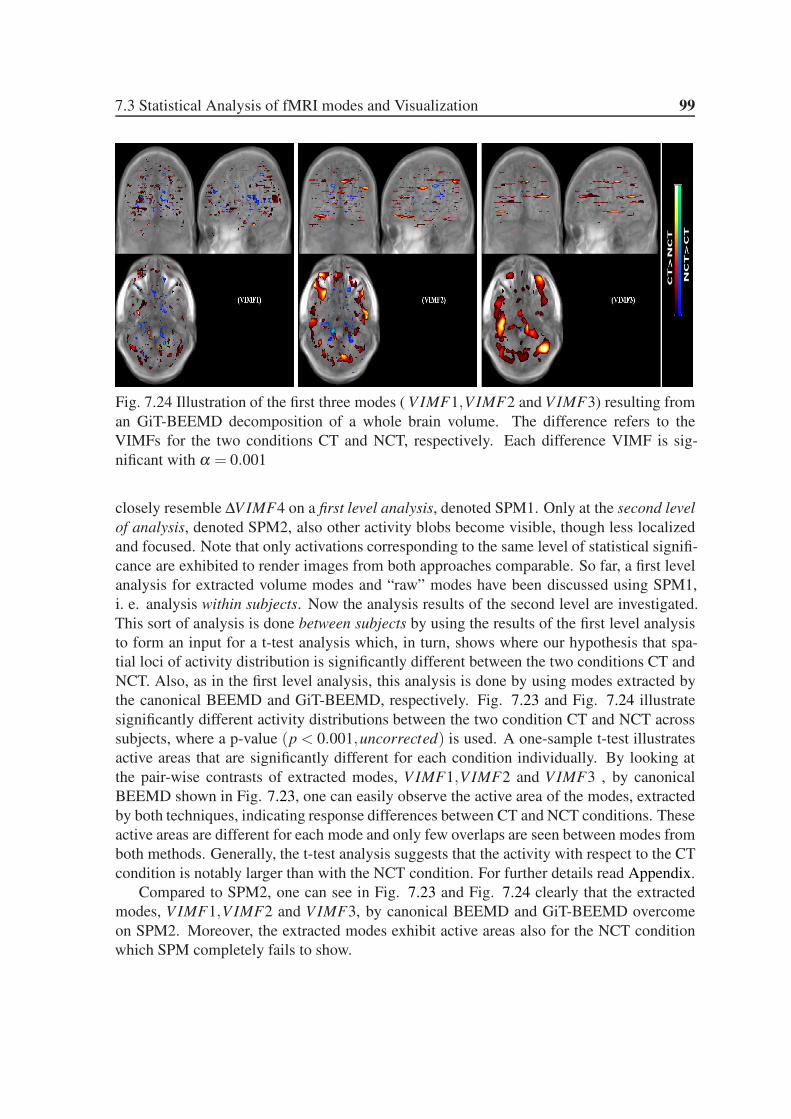
7.3 Statistical Analysis of fMRI modes and Visualization 99
Fig. 7.24 Illustration of the first three modes ( V IMF1,VIMF2 and VIMF3) resulting from
an GiT-BEEMD decomposition of a whole brain volume. The difference refers to the
VIMFs for the two conditions CT and NCT, respectively. Each difference VIMF is sig-
nificant with α = 0.001
closely resemble ∆V IMF4 on a first level analysis, denoted SPM1. Only at the second level
of analysis, denoted SPM2, also other activity blobs become visible, though less localized
and focused. Note that only activations corresponding to the same level of statistical signifi-
cance are exhibited to render images from both approaches comparable. So far, a first level
analysis for extracted volume modes and “raw” modes have been discussed using SPM1,
i. e. analysis within subjects. Now the analysis results of the second level are investigated.
This sort of analysis is done between subjects by using the results of the first level analysis
to form an input for a t-test analysis which, in turn, shows where our hypothesis that spa-
tial loci of activity distribution is significantly different between the two conditions CT and
NCT. Also, as in the first level analysis, this analysis is done by using modes extracted by
the canonical BEEMD and GiT-BEEMD, respectively. Fig. 7.23 and Fig. 7.24 illustrate
significantly different activity distributions between the two condition CT and NCT across
subjects, where a p-value (p < 0.001,uncorrected) is used. A one-sample t-test illustrates
active areas that are significantly different for each condition individually. By looking at
the pair-wise contrasts of extracted modes, V IMF1,VIMF2 and VIMF3 , by canonical
BEEMD shown in Fig. 7.23, one can easily observe the active area of the modes, extracted
by both techniques, indicating response differences between CT and NCT conditions. These
active areas are different for each mode and only few overlaps are seen between modes from
both methods. Generally, the t-test analysis suggests that the activity with respect to the CT
condition is notably larger than with the NCT condition. For further details read Appendix.
Compared to SPM2, one can see in Fig. 7.23 and Fig. 7.24 clearly that the extracted
modes, VIMF1,VIMF2 and VIMF3, by canonical BEEMD and GiT-BEEMD overcome
on SPM2. Moreover, the extracted modes exhibit active areas also for the NCT condition
which SPM completely fails to show.

7.4 Classification Results 100
Corresponding MNI coordinates of these localized activity blobs of the modes extracted
by BEEMD and GiT-BEEMD in case of a second level analysis are also collected in Tab.
A.3 and Tab. A.4. The corresponding activity distributions of the latter are shown in Fig.
A.3 and A.4, respectively (See in Appendix).
7.4 Classification Results
The baseline for classification performance of this work is the Voxels-as-Features (VAF)
approximation shown in Tab. 7.2, which uses all voxels in each raw image as a feature
vector. It is used as an input to the SVM-SMO as well as RF classifiers. The original feature
vector has 153,594 features. A leave-one-out cross-validation (LOOCV) strategy is used
and several metrics are used to measure the performance of the classifiers, namely accuracy
(acc), sensitivity (sens) and specificity (spec).
Tab. 7.2 Results of the baseline classification VAF.
Method Acc ± std Spec ± std Sens ± std
SVM-SMO 0.50±0.04 0.54±0.08 0.40±0.04
RF 0.32±0.02 0.29±0.02 0.35±0.03
7.4.1 Classification fMRI modes extracted by a canonical BEEMD
Here, two approaches for fMRI classification are presented in detail:
Approach I : As depicted in Fig. 7.25 (Top), the dimensionality reduction techniques
PCA, ICA and NMF are first applied to the whole dataset either raw data or the extracted
modes (VIMFs). Afterwards, data are projected onto the respective inherent coordinates.Then
the LOOCV procedure is employed using these projected data.
Approach II : As depicted in Fig. 7.25 (Bottom), the dimensionality techniques PCA,
ICA and NMF are applied to only the training dataset, either raw data or the extracted
modes (VIMFs), except one image at a time. The latter is used as a test image. This image
is then projected onto the basis vectors resulting from the training data. Afterwards, the
produced projected data of a test image is plug in as input to a classifier. In this way, the
LOOCV is used as well. Consequently, this approach is more robust and can be generalized.
Note, although the former approach could produce ultimate accuracies, it suffers from
serious drawbacks like over-fitting, as will be discussed more later on. Unfortunately, many
researchers do not pay much attention to such pitfalls. On the other hand, the latter, Ap-
proach II, could not reach to maximum accuracies but is more trust than other. Both ap-
proaches are dependent on extracted features during a pre-processing step, but Approach II
is more general than Approach I.
For each approach, classification of two data sets has been considered:

7.4 Classification Results 101
Fig. 7.25 Top: Illustration of the Approach I procedure for classification. Bottom: Illustra-
tion of the Approach II procedure for classification. Dot lines represent the optimization
process of classification framework.

7.4 Classification Results 102
• Projections onto principal directions of average volumes 〈Vsc(x,y,z)〉 deduced from
"raw" data and collected in an L×S matrix Zav.
• Projections onto principal directions of volume modes VIMFk,k = 1, . . . ,K deduced
either from a 2DBEEMD or a GiT-BEEMD decomposition of average volumes 〈V (x,y,z)〉and collected in an L×S matrix Zvm.
Also, in this section two experiments are discussed:
– Experiment 1: The VIMFs resulted from a canonical BEEMD are used without em-
ploying any filtering to take artifacts away.
– Experiment 2: Gaussian filtering is applied to the VIMFs before the feature generation
stage in order to deal with artifacts accompany with extracted modes from a canonical
BEEMD decomposition.
1 5 10 15 20 25 30 35
Principal Components ( PCs)
0
0.1
0.2
0.3
0.4
0.5
0.6
0.7
0.8
0.9
1
Variance Explained
Eginenvalues
Fig. 7.26 Normalized eigenvalue spectrum and related cumulative variance for vol-
ume mode VIMF3 after decomposition with PCA.
These projections are called orthogonal projections and are used as features for classi-
fication. The scree plot, see Fig. 7.26, illustrates the normalized eigenvalue spectrum and
related cumulative sum of variances for the most discriminative volume mode VIMF3. It
can be seen that the eigenvalue spectrum levels off after only L = 10 eigenvalues which
in total already explains roughly 80% of the data variance. The eigenvolumes, i. e. the
columns of matrix U , represent uncorrelated partial activity distributions in the brain. Fig.
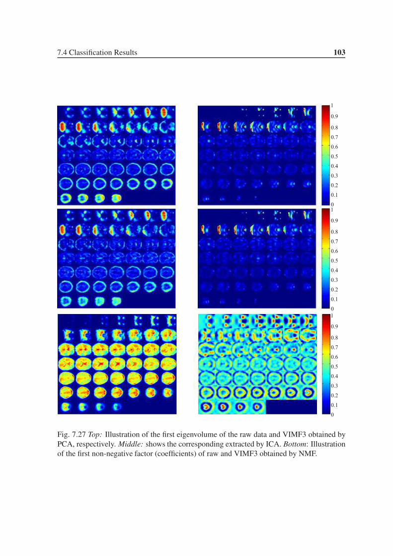
7.4 Classification Results 103
Fig. 7.27 Top: Illustration of the first eigenvolume of the raw data and VIMF3 obtained by
PCA, respectively. Middle: shows the corresponding extracted by ICA. Bottom: Illustration
of the first non-negative factor (coefficients) of raw and VIMF3 obtained by NMF.

7.4 Classification Results 104
7.27 illustrates the eigenvolume related with the second largest eigenvalue for both the raw
data and VIMF3, respectively. Both underline the relevance of the occipital area for contour
integration. However, the activity distribution provided by VIMF3 is much more focused
than in case of the raw data.
Given all orthogonal projections Z discussed above, a rotation matrix W is estimated.
The resulting independent projections, after re-ordering, are collected
• in an L×S matrix Sav in case of the projected "raw" data, or
• in an L×S matrix Svm in case of the projected volume modes.
Also, the basis vectors extracted by NMF are considered:
• in an L×S matrix Hav in case of metagenes represented "raw" data, or
• in an L×S matrix Hvm in case of the metagenes represented volume modes.
Either orthogonal (Zav,Zvm) and independent (Sav,Svm) projections or non-negative basis
vectors (Hav,Hvm) thus obtained have been input to either an RF or an SVM-SMO classifier.
Later on, the other types of SVM algorithm is employed. All are trained by adding one
feature at a time following a LOOCV strategy. Both RF and SVM-SMO with a sigmoidal
kernel are considered as stochastic algorithms, because Sequential Minimization Optimiza-
tion(SMO) breaks the problem into sub-problems and the initial weight of the sigmoidal
kernel is random and RF uses a bagging technique internally. On the contrary, the alter-
native SVM methods, SVM-QP and SVM-LS, are deterministic algorithms. SVM-SMO
training can be performed efficiently by applying a SMO technique which breaks the large
quadratic programming (QP) problem into a sequence of smaller QP sub-problems which
can be solved analytically [138]. For both stochastic classifiers, training and testing was
repeated 10 times, later on only once for the deterministic classifiers, while permuting the
whole data set randomly, and an LOOCV strategy was invoked to obtain reliable results.
Several metrics were used to measure the performance of the classifiers, namely accuracy
(acc), sensitivity (sens), specificity (spec) and the Receiver Operating Characteristic (ROC)
curve. This procedure is applied using both approaches, Approach I and Approach II.
7.4.1.1 Raw data
Approach I : first "raw" features, i. e. the projections Zav of average volumes, resulting
from "raw" data, onto their principal directions have been fed to an SVM-SMO classifier
yielding an average accuracy acc = 0.75±0.03, an average specificity spec = 0.72±0.03
and an average sensitivity sens = 0.77±0.05 (see first column of Fig. 7.28). These figures
have been obtained by varying the number of principal components L and choosing the
optimal number of PCs (L = 10) according to the highest accuracy achieved.
Next, the same "raw" features have been fed to an RF classifier resulting in an average
accuracy acc = 0.66±0.04, an average specificity spec = 0.66±0.07 and an average sensi-
tivity sens= 0.65±0.07. These results have been obtained with the total number of features
(L = 38) according to the highest accuracy obtained.

7.4 Classification Results 105
The orthogonal projections of the raw data onto the PCs leave some statistical depen-
dencies, hence ICA was applied to remove the latter. The resulting independent projections
Sav were again fed into the SVM-SMO classifier resulting in the following statistical mea-
sures: an average accuracy acc = 0.64± 0.02, an average specificity spec = 0.64± 0.02
and an average sensitivity sens = 0.64±0.05. Then, the same ICs (features) have been fed
to an RF classifier yielding an average accuracy acc = 0.66± 0.00, an average specificity
spec = 0.68±0.00 and an average sensitivity sens = 0.63±0.00.
Besides, NMF is a parts-based technique while PCA and ICA are global techniques.
This behavior is reflected in the bases obtained by these techniques. So, the basis vectors,
resulting from NMF, were used as input to an SVM-SMO classifier and resulted in an aver-
age accuracy acc = 0.80±0.06, an average specificity spec = 0.77±0.10 and an average
sensitivity sens = 0.88± 0.04. These results have been obtained with the optimal number
of basis vector Hav (L = 17) according to the highest accuracy achieved. Then, the same
basis vectors (features) have been fed to an RF classifier resulting in an average accuracy
acc = 0.42± 0.01, an average specificity spec = 0.40± 0.02 and an average sensitivity
sens = 0.45±0.02.
Approach II : the "raw" features, i. e. the projections of the average volumes training data
Ztrainav, have been used to train an SVM-SMO classifier. Afterwards, the test data Ztestav
projected on the eigenvector resulted from training phase. Then the produced projected
data of new, formerly unseen average volumes is tested by the trained classifier. This is
performed M−1 times, based on LOOCV, and yielded an average accuracy acc = 0.74±0.00, an average specificity spec= 0.75±0.00 and an average sensitivity sens= 0.72±0.00.
These results were obtained by varying the number of principal components L and choosing
the optimal number of PCs (L = 16) according to the highest accuracy achieved. Next,
the same procedure was applied to an RF classifier and resulted in an average accuracy
acc = 0.60± 0.00, an average specificity spec = 0.52± 0.03 and an average sensitivity
sens = 0.57± 0.00. These results have been obtained with the total number of features
(L = 38) according to the highest accuracy obtained.
The orthogonal projections of the raw training data onto the PCs leave some statistical
dependencies, hence ICA was applied to remove the latter. The resulting independent pro-
jections Stestav, fed into the SVM-SMO classifier, resulted in the following statistical mea-
sures: an average accuracy acc = 0.73± 0.03 , an average specificity spec = 0.72± 0.01
and an average sensitivity sens = 0.74± 0.00 . Then, the same ICs (features) have been
fed to an RF classifier getting an average accuracy acc = 0.65±0.00, an average specificity
spec = 0.67±0.01 and an average sensitivity sens = 0.63±0.00.
Also, "raw" features were extracted by applying an NMF and used as input to an SVM-
SMO classifier and resulting in an average accuracy acc= 0.73±0.03, an average specificity
spec = 0.74±0.03 and an average sensitivity sens = 0.80±0.03. These results have been
obtained with the optimal number of basis vectors Htrainav and Htestav (L = 10) according
to the highest accuracy achieved. But, when the same basis vectors (features) have been fed
into an RF classifier, no more than by chance 50 % resulted.

7.4 Classification Results 106
Note, though, using Approach I, the results provided in case of NMF were superior to
those obtained when using PCA and ICA, while the latter achieved results superior to those
of an NMF application using Approach II. This means that generalizing the model should
be done in combination with PCA or ICA rather than NMF when fMRI data is considered.
7.4.1.2 Volume Image Modes
Approach I : obviously projections Zav of "raw" data yield poor classification accuracies
only. A canonical BEEMD decomposition of the "raw" data set resulted in six volume
modes V IMFk, k = 1, . . . ,K = 6 which might have been further processed by a Gaussian
smoothing filter to remove certain streak artifacts. Afterwards, the corresponding orthogonal
(Zvm) or independent (Svm) projections or the NMF basis vectors (metagenes) of the VIMFs
(Hvm) were used as appropriate features and have been fed into either an SVM or an RF
classifier trained to differentiate between the stimulus/response conditions CT and NCT.
Raw data VIMF1 VIMF2 VIMF3 VIMF4 VIMF5 VRes.0
0.1
0.2
0.3
0.4
0.5
0.6
0.7
0.8
0.9
1
Acc
ura
cy
Raw data and modes
Fig. 7.28 Boxplot comparing the accuracy achieved by the SVM classifier using
projections of the "raw" data as well as of the volume modes (VIMFs) resulting
from a canonical BEEMD analysis with subsequent Gaussian smoothing.
An exhaustive experimental evaluation of the classifiers has been conducted, having
as input either Zvm, Svm or metagenes Hvm. Here the number of features L was also a
variable for the SVM classifier, but kept constant to L = 38 in case of the RF classifier.
The results show that an SVM classifier achieves the best performance with L = 11± 2
input features. In addition, both classifiers exhibit their highest performance with features
extracted from VIMF3. Even the remaining modes, with the exception of VIMF1, also
present better results than the raw data in many cases. Furthermore, the quality of the

7.4 Classification Results 107
5 6 7 8 9 10 11 12 13 14 15 37
Number of selected components (PCs)
0
0.1
0.2
0.3
0.4
0.5
0.6
0.7
0.8
0.9
1
Acc
., S
pec
., S
ens.
IMF1Acc
IMF3Acc
IMF1Spe
IMF3Spe
IMF1Sens
IMF3Sens
Fig. 7.29 Variation of statistical measures, obtained with SVM and Gaussian fil-
tering, with the number of principal components extracted from volume modes
V IMF3 and VIMF1, respectively.
0 0.2 0.4 0.6 0.8 1
False Positive Rate (1-Specificity)
0
0.1
0.2
0.3
0.4
0.5
0.6
0.7
0.8
0.9
1
Tru
e P
osi
tiv
e R
ate
(S
ensi
tiv
ity
)
ROC curve (SVM)
VIMF1
VIMF2
VIMF3
VIMF4
VIMF5
VRes.
Raw Data
0 0.2 0.4 0.6 0.8 1
False Positive Rate (1-Specificity)
0
0.1
0.2
0.3
0.4
0.5
0.6
0.7
0.8
0.9
1
Tru
e P
osi
tiv
e R
ate
(S
ensi
tiv
ity
)
ROC curve (RF)
VIMF1
VIMF2
VIMF3
VIMF4
VIMF5
VRes.
Raw Data
Fig. 7.30 Receiver Operating Characteristics (ROC) from all six volume modes (VIMFs)
for Experiment 2. Left: ROC curves of VIMFs resulting from an SVM classification.
Right: ROC curves of VIMFs resulting from an RF classification.

7.4 Classification Results 108
classifier behavior was similar using metamodes or orthogonal features. The NMF was
tested with different 2 ≤ l ≤ 18. For more than 18 features, the algorithm converges to
a solution of lower rank than L, which may indicate that the result is not optimal. Then
the classifier were applied to each l separately and the best results are reported. Moreover,
the performance of the classifiers is better with orthogonal features than with independent
features. And the linear filtering, applied to the VIMFs, also has a positive impact on the
performance. Best results are summarized in Tab. 7.3, Tab. 7.4, Tab. 7.5 , Tab. 7.6,
Tab. 7.8 and Tab. 7.7. Among all modes, the highest accuracy is performed with V IMF3
except in case of combining random forest classifier with NMF, the highest accuracy is
done with V IMF4. Also, from results shown in tables, one can see that combining SVM
with NMF has achieve the highest classification accuracy in exp. 1 ,with Acc.= 0.83±0.06.
With exp. 2, combining SVM with PCA performed slightly better than the former with
Acc. = 0.82±0.07. Again, although the other combination of classifiers either SVM or RF
has generated good classification accuracies as well, only the surprising results come from
the combination RF with NMF , the classification accuracy with all modes is not better than
by-chance. Thus, such combination should be further investigated in future work.
Fig. 7.28 illustrates the accuracy achieved with all VIMFs resulting from an SVM classi-
fier and Gaussian filtering (exp. 2). Fig. 7.29 provides a more complete picture. It illustrates
the dependence of accuracy (acc), specificity (spec) and sensitivity (sens) on the number of
PCs extracted, hence the dimension of the feature subspace. These statistical measures
were achieved using features, i. e. projections, of the first ZV IMF1 and third ZV IMF3 vol-
ume modes, respectively. While VIMF1 always represents a small scale, VIMF3 exhibits
textures which provide the most discriminative features for contour vs non-contour stim-
uli. As an additional statistical measure, Fig. 7.30 presents the related Receiver Operating
Characteristic (ROC) curves for all VIMFs and average volumes resulting from a data de-
composition involving Gaussian filtering (exp. 2). The related area-under-curve (AUC)
indicator yields AUC = 0.86 and AUC = 0.80 in case of VIMF3 classified with SVM and
RF, respectively. Corresponding measures in case of VIMF4 amount to AUC = 0.82 and
AUC = 0.78, respectively.
Tab. 7.3 Statistical measures evaluating classification results obtained by PCA and SVM clas-
sifier either without (exp. 1) or with (exp. 2) applying a linear Gaussian filter to the VIMFs
(Approach I).
SVM
experiment 1 experiment 2
Acc ± std Spec ± std Sens ± std Acc ± std Spec ± std Sens ± std
VIMF1 0.72±0.05 0.69±0.06 0.75±0.56 0.66±0.05 0.62±0.07 0.70±0.07
VIMF2 0.79±0.06 0.79±0.04 0.78±0.10 0.75±0.05 0.75±0.04 0.75±0.09
VIMF3 0.80±0.05 0.82±0.07 0.79±0.05 0.81±0.04 0.84±0.04 0.78±0.05
VIMF4 0.79±0.06 0.83±0.08 0.75±0.08 0.77±0.03 0.75±0.04 0.77±0.05
VIMF5 0.74±0.03 0.75±0.04 0.72±0.07 0.72±0.11 0.66±0.10 0.77±0.14
VRes. 0.77±0.03 0.74±0.07 0.79±0.04 0.72±0.03 0.71±0.07 0.73±0.04

7.4 Classification Results 109
Tab. 7.4 Statistical measures evaluating classification results obtained with PCA and an RF
classifier either without (exp. 1) or with (exp. 2) applying a linear Gaussian filter to the
VIMFs (Approach I).
RF
experiment 1 experiment 2
Acc ± std Spec ± std Sens ± std Acc ± std Spec ± std Sens ± std
VIMF1 0.48±0.02 0.47±0.03 0.50±0.03 0.53±0.04 0.56±0.04 0.51±0.04
VIMF2 0.58±0.02 0.63±0.03 0.53±0.03 0.51±0.02 0.48±0.03 0.53±0.03
VIMF3 0.75±0.02 0.79±0.04 0.71±0.04 0.78±0.02 0.81±0.04 0.75±0.04
VIMF4 0.71±0.02 0.71±0.03 0.71±0.03 0.73±0.02 0.70±0.03 0.77±0.03
VIMF5 0.61±0.02 0.57±0.04 0.65±0.04 0.47±0.01 0.46±0.02 0.48±0.02
VRes. 0.65±0.04 0.68±0.05 0.61±0.05 0.52±0.03 0.57±0.04 0.47±0.04
Tab. 7.5 Statistical measures evaluating classification results obtained with ICA and an SVM
classifier either without (exp. 1) or with (exp. 2) applying a linear Gaussian filter to the
VIMFs (Approach I).
SVM
experiment 1 experiment 2
Acc ± std Spec ± std Sens ± std Acc ± std Spec ± std Sens ± std
VIMF1 0.67±0.01 0.64±0.03 0.70±0.04 0.64±0.03 0.65±0.02 0.62±0.05
VIMF2 0.69±0.04 0.70±0.07 0.68±0.03 0.70±0.03 0.70±0.05 0.69±0.04
VIMF3 0.76±0.03 0.78±0.06 0.74±0.03 0.73±0.01 0.68±0.00 0.77±0.02
VIMF4 0.70±0.03 0.67±0.04 0.73±0.08 0.72±0.04 0.68±0.04 0.76±0.04
VIMF5 0.70±0.06 0.72±0.06 0.68±0.10 0.63±0.02 0.63±0.04 0.64±0.04
VRes. 0.60±0.02 0.66±0.04 0.53±0.02 0.62±0.05 0.67±0.03 0.56±0.10
Tab. 7.6 Statistical measures evaluating classification results obtained with ICA and an RF
classifier either without (exp. 1) or with (exp. 2) applying a linear Gaussian filter to the
VIMFs (Approach I).
RF
experiment 1 experiment 2
Acc ± std Spec ± std Sens ± std Acc ± std Spec ± std Sens ± std
VIMF1 0.39±0.01 0.41±0.03 0.37±0.02 0.44±0.00 0.52±0.00 0.36±0.00
VIMF2 0.56±0.02 0.59±0.00 0.54±0.05 0.42±0.03 0.44±0.02 0.50±0.04
VIMF3 0.70±0.02 0.70±0.03 0.66±0.03 0.76±0.03 0.77±0.04 0.76±0.03
VIMF4 0.61±0.02 0.52±0.02 0.65±0.02 0.74±0.02 0.74±0.04 0.74±0.04
VIMF5 0.55±0.04 0.56±0.07 0.55±0.03 0.40±0.00 0.38±0.00 0.42±0.00
VRes. 0.66±0.01 0.68±0.00 0.65±0.02 0.53±0.00 0.47±0.00 0.58±0.00
In face, though some results, in Approach I, looks reasonable, this approach is considers
as unstable model in general. Later on, especially under optimization framework, the effect
of over-fitting problem wit this approach will be seen clearly.

7.4 Classification Results 110
Tab. 7.7 Statistical measures evaluating classification results obtained with NMF and an SVM
classifier either without (exp. 1) or with (exp. 2) applying a linear Gaussian filter to the
VIMFs (Approach I).
SVM
experiment 1 experiment 2
Acc ± std Spec ± std Sens ± std Acc ± std Spec ± std Sens ± std
VIMF1 0.80±0.07 0.84±0.04 0.76±0.10 0.77±0.10 0.79±0.08 0.76±0.14
VIMF2 0.80±0.04 0.80±0.04 0.80±0.06 0.78±0.07 0.81±0.12 0.75±0.05
VIMF3 0.83±0.06 0.77±0.10 0.88±0.04 0.80±0.03 0.79±0.04 0.81±0.04
VIMF4 0.80±0.04 0.76±0.06 0.83±0.04 0.80±0.04 0.77±0.04 0.82±0.07
VIMF5 0.77±0.02 0.81±0.04 0.73±0.03 0.83±0.04 0.82±0.06 0.85±0.04
VRes. 0.81±0.06 0.76±0.09 0.87±0.08 0.84±0.05 0.84±0.08 0.84±0.07
Tab. 7.8 Statistical measures evaluating classification results obtained with NMF and an RF
classifier either without (exp. 1) or with (exp. 2) applying a linear Gaussian filter to the
VIMFs (Approach I).
RF
experiment 1 experiment 2
Acc ± std Spec ± std Sens ± std Acc ± std Spec ± std Sens ± std
VIMF1 0.36±0.01 0.36±0.01 0.35±0.02 0.42±0.00[1] 0.47±0.00 0.36±0.00
VIMF2 0.44±0.00 0.42±0.00 0.47±0.00 0.47±0.00[1] 0.42±0.00 0.52±0.00
VIMF3 0.39±0.00 0.42±0.00 0.37±0.00 0.53±0.00[1] 0.63±0.00 0.42±0.00
VIMF4 0.58±0.00 0.63±0.00 0.52±0.00 0.39±0.00[1] 0.36±0.00 0.42±0.00
VIMF5 0.44±0.00 0.42±0.00 0.47±0.00 0.47±0.00[1] 0.47±0.00 0.47±0.00
VRes. 0.52±0.00 0.52±0.00 0.52±0.00 0.47±0.00[1] 0.47±0.00 0.47±0.00
Approach II : from Tab. 7.9, Tab. 7.12, Tab. 7.10, Tab. 7.13 and Tab. 7.11, one can
see clearly how the SVM-SMO and RF classifiers yield, for specific modes and in case of
PCA and ICA, slightly better classification accuracies using Approach I than Approach II,
and this holds even more so when NMF-based features were employed. Although results
achieved with Approach I look better, those obtained with Approach II are more robust and
more generally valid than with Approach I. Following one can see how the optimization
process will enhance the accuracy of Approach I strongly but still stay unreliable. As Ap-
proach II, the corresponding orthogonal (Zvm) and independent (Svm) projections, or the
non-negative factors (Hvm) of the VIMFs were used as appropriate features and have been
fed into either an SVM-SMO or an RF classifier trained to differentiate the stimulus/re-
sponse conditions CT and NCT. An exhaustive experimental evaluation of the classifiers
has been conducted, having as input (Zvm) , (Svm) or (Hvm). Here the number of features
L was almost similar to a variable considered in Approach I for the SVM classifier, and
reduced dramatically in case of RF classifier only with (Hvm) , L = 1± 2 . Note again,
Approach I may produce a high accuracy but it does not generalize properly like Approach
II. Thus the high accuracy achieved on the training samples has to be considered overfitting.
Hence, again Approach II is more realistic, robust and reliable.

7.4 Classification Results 111
Tab. 7.9 Statistical measures evaluating classification results obtained by PCA and an SVM
classifier either without (exp. 1) or with (exp. 2) applying a linear Gaussian filter to the
VIMFs (Approach II).
SVM
experiment 1 experiment 2
Acc ± std Spec ± std Sens ± std Acc ± std Spec ± std Sens ± std
VIMF1 0.71±0.00 0.68±0.01 0.74±0.00 0.76±0.02 0.78±0.03 0.73±0.01
VIMF2 0.76±0.00 0.77±0.03 0.74±0.01 0.71±0.00 0.74±0.01 0.67±0.03
VIMF3 0.83±0.02 0.82±0.04 0.84±0.00 0.82±0.00 0.84±0.01 0.78±0.01
VIMF4 0.81±0.03 0.77±0.04 0.83±0.01 0.79±0.00 0.85±0.03 0.73±0.01
VIMF5 0.76±0.00 0.73±0.03 0.79±0.01 0.79±0.00 0.88±0.03 0.69±0.01
VRes. 0.80±0.04 0.81±0.08 0.79±0.00 0.76±0.00 0.73±0.03 0.79±0.00
Tab. 7.10 Statistical measures evaluating classification results obtained by ICA and an SVM
classifier either without (exp. 1) or with (exp. 2) applying a linear Gaussian filter to the
VIMFs (Approach II).
SVM
experiment 1 experiment 2
Acc ± std Spec ± std Sens ± std Acc ± std Spec ± std Sens ± std
VIMF1 0.76±0.01 0.83±0.01 0.68±0.01 0.65±0.02 0.58±0.00 0.72±0.04
VIMF2 0.66±0.02 0.57±0.03 0.73±0.01 0.76±0.00 0.94±0.01 0.59±0.01
VIMF3 0.74±0.05 0.73±0.03 0.76±0.08 0.79±0.00 0.79±0.00 0.78±0.01
VIMF4 0.69±0.00 0.84±0.01 0.53±0.00 0.74±0.00 0.74±0.00 0.74±0.01
VIMF5 0.76±0.02 0.89±0.01 0.62±0.03 0.81±0.01 0.73±0.03 0.89±0.00
VRes. 0.69±0.05 0.71±0.06 0.67±0.04 0.66±0.02 0.69±0.03 0.64±0.01
Tab. 7.11 Statistical measures evaluating classification results obtained with NMF and an
SVM classifier either without (exp. 1) or with (exp. 2) applying a linear Gaussian filter to the
VIMFs (Approach II).
SVM
experiment 1 experiment 2
Acc ± std Spec ± std Sens ± std Acc ± std Spec ± std Sens ± std
VIMF1 0.64±0.01 0.57±0.02 0.71±0.03 0.57±0.00 0.39±0.15 0.76±0.15
VIMF2 0.67±0.13 0.78±0.10 0.55±0.15 0.71±0.03 0.75±0.02 0.68±0.10
VIMF3 0.71±0.10 0.70±0.07 0.71±0.13 0.68±0.03 0.59±0.13 0.76±0.05
VIMF4 0.68±0.06 0.58±0.10 0.77±0.02 0.72±0.02 0.61±0.07 0.82±0.02
VIMF5 0.70±0.07 0.68±0.10 0.71±0.05 0.81±0.05 0.80±0.07 0.81±0.05
VRes. 0.76±0.03 0.73±0.00 0.72±0.07 0.74±0.00 0.71±0.05 0.75±0.07
From the discussion of the two approaches above, stable results have clearly been pro-
duced by combining PCA with an SVM classifier. So, henceforth, further optimization are
performed using PCA and SVM, only.

7.4 Classification Results 112
Tab. 7.12 Statistical measures evaluating classification results obtained by PCA and RF clas-
sifier either without (exp. 1) or with (exp. 2) applying a linear Gaussian filter to the VIMFs
(Approach II).
RF
experiment 1 experiment 2
Acc ± std Spec ± std Sens ± std Acc ± std Spec ± std Sens ± std
VIMF1 0.45±0.00 0.52±0.01 0.37±0.00 0.60±0.00 0.47±0.00 0.73±0.00
VIMF2 0.48±0.00 0.47±0.00 0.42±0.00 0.45±0.00 0.58±0.00 0.32±0.00
VIMF3 0.52±0.00 0.42±0.00 0.62±0.00 0.55±0.00 0.58±0.00 0.53±0.00
VIMF4 0.31±0.00 0.36±0.04 0.26±0.01 0.57±0.00 0.57±0.00 0.57±0.00
VIMF5 0.34±0.00 0.31±0.00 0.36±0.00 0.42±0.00 0.42±0.00 0.42±0.00
VRes. 0.42±0.04 0.42±0.08 0.42±0.00 0.44±0.00 0.47±0.03 0.42±0.00
Tab. 7.13 Statistical measures evaluating classification results obtained by ICA and RF clas-
sifier either without (exp. 1) or with (exp. 2) applying a linear Gaussian filter to the VIMFs
(Approach II).
RF
experiment 1 experiment 2
Acc ± std Spec ± std Sens ± std Acc ± std Spec ± std Sens ± std
Raw 0.65±0.00 0.67±0.01 0.63±0.00 − − −VIMF1 0.49±0.00 0.41±0.03 0.58±0.01 0.50±0.02 0.53±0.03 0.47±0.01
VIMF2 0.52±0.01 0.47±0.00 0.57±0.03 0.57±0.02 0.58±0.00 0.56±0.04
VIMF3 0.58±0.01 0.53±0.01 0.64±0.01 0.63±0.00 0.68±0.00 0.58±0.00
VIMF4 0.39±0.00 0.42±0.01 0.36±0.00 0.60±0.01 0.68±0.01 0.52±0.01
VIMF5 0.63±0.00 0.57±0.01 0.68±0.03 0.44±0.01 0.25±0.03 0.63±0.00
VRes. 0.65±0.05 0.73±0.01 0.58±0.00 0.57±0.01 0.56±0.03 0.57±0.00
7.4.2 Optimization of Classification Accuracy
In the previous section principal component analysis was used to reduce the number of
input dimensions to the classifiers. The principal components were ranked in decreasing
order according to the amount of variance accounted for in the original data (i. e., based on
the eigenvalues). The final set of principal components used was determined empirically
by adding one principal component at a time to the classifier, training the classifier, and
then evaluating its performance using LOOCV. Then, the set of principal components that
produced the best performance were reported. In case of RF, the importance of features eval-
uated by the gini index (GI) as an indication that the order of feature importance does not
conform to the order of features according to the amount of the variance explained. Hence,
ranking the principal components according to the amount of variance they account for,
may not reflect how well they discriminate between classes. Therefore, another procedure
is also evaluated to determine which of the principal components have the most discrimi-
nating power. This procedure is a stepwise add-on procedure based on adding the principal
component that improves the performance of the classifiers. This ranking of the principal

7.4 Classification Results 113
Fig. 7.31 Illustration of the normalized amount of total variance of explained by PCA, and
the most discriminant principal components ranked by t-test for all modes, K = 1 . . .6, re-
spectively.

7.4 Classification Results 114
components was determined by first training a classifier on all Z = 38 principal components,
in case of Approach I, and M− 1 in case of Approach II, using a random forest. Another
classifier was then created by taking the ranked features from the initial classifier by the
Gini index measure, one at a time, and testing using LOOCV. The principal component that
performed the best was next used with the remaining features one at a time, and now the
pair of features that gave the best performance was used with the remaining features. This
procedure was carried out by incrementally adding principal components to the classifier
based on their ability to improve performance. Eventually, one can see clearly the effect of
ordering features in terms of their discriminating power. In addition to the Gini Index, in this
chapter other common strategies are descried, for feature selection like T-test, information
gain (IG) and Fisher score (FS), which were introduced in the chapter about classification.
These feature selection techniques are independent of the classifier used, except the Gini
index. In this section the effect of feature selection techniques, to help in improving the
accuracy, is shown. Following, the classification performance of other traditional different
types of SVM methods is compared to the SVM-SMO. Finally, the SVM-SMO classifier
parameters are tuned using a grid search strategy.
Approach I : Tab. 7.14 shows how the accuracy, achieved with an SVM-SMO classi-
fier, has been enhanced notably with all VIMFs, especially with VIMF4, which reached an
accuracy of Acc. = 0.94 with all feature selection methods except the Gini index, which
achieved Acc. = 0.92 . Similarly, with an RF classifier the accuracy is enhanced dramati-
cally with all modes. The best accuracy was almost similar with VIMF3 and VIMF4 in case
of exp. 1, which was equal to Acc. = 0.82, and only VIMF4 in case of exp. 2 and, which
equal to Acc. = 0.89. On the other hand, the worse accuracy using SVM and Gini Index is,
Acc. = 0.81, performed with V IMF1 in case of exp. 1 and with V IMF2 in case of exp. 2,
Acc. = 0.82. With SVM and Fisher Score, the worse accuracy, in exp. 1, is reported with
the residuum, Acc. = 0.76, and V IMF4 with accuracy Acc. = 0.84 in case of exp. 2. With
SVM and Information Gain, VIMF1 reports less accuracy among others with Acc. = 0.82
in case of exp. 1 while V IMF3 with Acc. = 0.83 in case of exp. 2. Finally, with SVM and
T-test, V IMF2 achieves the worse accuracy with Acc. = 0.79 in case of exp. 1 and V IMF1
with Acc. = 0.79 in case of exp. 2. Likewise, for RF with the different features selection,
Tab. 7.15 shows the the optimal accuracies with bold font and the worse accuracies also
are easily recognizable. In addition to the sigmoidal kernel, the other common kernels are
used. Tab. 7.16 shows the effect of the linear, quadratic, Gaussian and polynomial kernel,
respectively. One can see that with the linear kernel, the accuracy achieved with all modes
in this approach reached the maximum Acc. = 1.00. With other kernels, the best accuracy
was achieved with VIMF3 and VIMF4 amounting to Acc.= 0.92±0.04. In exp. 1, one can
see in many cases that V IMF3 and VIMF4 provide the same accuracy, for example with
RF and T-test the accuracy of both is Acc. = 0.82. The values between square brackets in
Tab. 7.14, Tab. 7.15 and Tab. 7.16, as well in other tables throughout this work, show the
number of selected features for an optimal performance, and the first column indicates the
proper mode.

7.4 Classification Results 115
In summary, from Tab. 7.14, the highest classification accuracies, using PCA and fea-
tures selection techniques with either SVM for Approach I, are:
• in exp. 1 with FS, the highest accuracy is 0.94 for V IMF4,
• in exp. 1 with IG, the highest accuracy is 0.94 for VIMF4,
• in exp. 1 with T-test, the highest accuracy is 0.94 for VIMF4 as well,
• and in exp. 2 with GI, the highest accuracy is 0.89 for V IMF3 and VIMF4.
Correspondingly, from Tab. 7.15, the highest classification accuracies, using PCA and fea-
tures selection techniques with either RF for Approach I, are:
• in exp. 1 with GI and T-test, the highest accuracy is 0.82 for VIMF3 and V IMF4,
• in exp. 1 with T-test, the highest accuracy is 0.82 for VIMF3 and V IMF4,
• in exp. 2 with GI, FS, IG and T-test, the highest accuracy is 0.89 for V IMF4.
Tab. 7.14 Statistical measures evaluating classification results obtained by PCA and SVM
classifier either with (exp. 1) or with (exp. 2) applying a linear Gaussian filter to the VIMFs.
The selection features are employed to order the extracted features (Approach I).
SVM
experiment 1 experiment 2
Feature Selection modes Acc ± std Spec ± std Sens ± std Acc ± std Spec ± std Sens ± std
VIMF1 0.86±0.02[3] 0.89±0.05 0.84±0.00 0.88±0.06[17] 0.88±0.09 0.88±0.03
GI VIMF2 0.85±0.05[16] 0.85±0.06 0.85±0.07 0.82±0.06[17] 0.85±0.05 0.78±0.09
VIMF3 0.83±0.06[16] 0.79±0.06 0.83±0.05 0.89±0.01[4] 0.87±0.02 0.85±0.01
VIMF4 0.92±0.00[4] 0.94±0.00 0.89±0.00 0.89±0.01[2] 0.89±0.00 0.86±0.02
VIMF5 0.89±0.04[9] 0.88±0.06 0.91±0.04 0.83±0.08[18] 0.78±0.10 0.87±0.07
VRes. 0.81±0.03[13] 0.79±0.03 0.83±0.04 0.86±0.07[25] 0.87±0.01 0.86±0.05
VIMF1 0.81±0.04[12] 0.80±0.07 0.82±0.04 0.88±0.01[6] 0.88±0.02 0.88±0.03
VIMF2 0.79±0.02[8] 0.80±0.02 0.77±0.06 0.88±0.03[20] 0.90±0.05 0.85±0.02
FS VIMF3 0.83±0.06[21] 0.80±0.06 0.85±0.08 0.86±0.06[21] 0.87±0.08 0.84±0.09
VIMF4 0.94±0.01[6] 0.95±0.02 0.94±0.02 0.84±0.00[1] 0.89±0.00 0.79±0.00
VIMF5 0.83±0.07[4] 0.88±0.06 0.78±0.09 0.87±0.03[6] 0.87±0.02 0.87±0.02
VRes. 0.76±0.00[8] 0.79±0.00 0.74±0.00 0.88±0.03[8] 0.87±0.04 0.88±0.04
VIMF1 0.82±0.03[4] 0.88±0.04 0.77±0.04 0.87±0.03[5] 0.85±0.03 0.90±0.04
VIMF2 0.83±0.04[17] 0.85±0.05 0.81±0.04 0.86±0.05[21] 0.88±0.06 0.84±0.09
IG VIMF3 0.85±0.03[12] 0.86±0.04 0.85±0.04 0.83±0.03[17] 0.79±0.09 0.86±0.07
VIMF4 0.94±0.03[7] 0.96±0.03 0.91±0.04 0.86±0.03[20] 0.87±0.07 0.86±0.06
VIMF5 0.85±0.03[16] 0.85±0.06 0.85±0.04 0.84±0.03[9] 0.80±0.01 0.89±0.05
VRes. 0.85±0.03[11] 0.86±0.04 0.87±0.04 0.88±0.04[6] 0.87±0.04 0.88±0.04
VIMF1 0.82±0.03[4] 0.88±0.04 0.77±0.04 0.79±0.02[5] 0.89±0.03 0.69±0.03
VIMF2 0.79±0.00[8] 0.80±0.02 0.77±0.06 0.87±0.03[20] 0.90±0.05 0.85±0.02
T-test VIMF3 0.83±0.06[21] 0.80±0.06 0.85±0.08 0.87±0.06[21] 0.87±0.08 0.84±0.09
VIMF4 0.94±0.01[6] 0.95±0.02 0.93±0.02 0.84±0.00[1] 0.89±0.00 0.79±0.00
VIMF5 0.87±0.06[9] 0.85±0.10 0.91±0.05 0.80±0.04[17] 0.80±0.07 0.81±0.07
VRes. 0.83±0.07[8] 0.81±0.06 0.87±0.09 0.88±0.04[5] 0.90±0.04 0.88±0.07

7.4 Classification Results 116
Tab. 7.15 Statistical measures evaluating classification results obtained by PCA and RF clas-
sifier either with (exp. 1) or with (exp. 2) applying a linear Gaussian filter to the VIMFs. The
selection features are employed to order the extracted features (Approach I).
RF
experiment 1 experiment 2
Feature Selection modes Acc ± std Spec ± std Sens ± std Acc ± std Spec ± std Sens ± std
VIMF1 0.74±0.02[3] 0.77±0.02 0.71±0.03 0.79±0.02[5] 0.89±0.03 0.69±0.03
VIMF2 0.69±0.01[3] 0.73±0.00 0.74±0.03 0.71±0.00[4] 0.74±0.00 0.69±0.01
GI VIMF3 0.82±0.05[6] 0.84±0.00 0.79±0.01 0.84±0.01[7] 0.83±0.03 0.84±0.00
VIMF4 0.82±0.00[3] 0.74±0.00 0.89±0.00 0.89±0.00[4] 0.89±0.00 0.89±0.00
VIMF5 0.76±0.00[4] 0.87±0.06 0.91±0.04 0.76±0.01[7] 0.79±0.00 0.73±0.03
VRes. 0.76±0.00[8] 0.79±0.00 0.74±0.00 0.88±0.03[8] 0.88±0.04 0.87±0.03
VIMF1 0.81±0.01[5] 0.83±0.02 0.79±0.00 0.76±0.02[3] 0.79±0.04 0.74±0.00
VIMF2 0.74±0.01[7] 0.74±0.00 0.75±0.02 0.72±0.03[7] 0.70±0.02 0.74±0.00
FS VIMF3 0.81±0.01[18] 0.84±0.02 0.79±0.02 0.84±0.02[9] 0.85±0.04 0.84±0.00
VIMF4 0.81±0.00[3] 0.79±0.00 0.84±0.01 0.89±0.00[10] 0.89±0.00 0.89±0.00
VIMF5 0.80±0.01[7] 0.68±0.05 0.91±0.00 0.76±0.02[6] 0.78±0.02 0.74±0.03
VRes. 0.76±0.00[8] 0.79±0.00 0.74±0.00 0.85±0.02[8] 0.79±0.03 0.91±0.03
VIMF1 0.80±0.01[3] 0.84±0.00 0.75±0.02 0.88±0.01[6] 0.88±0.01 0.788±0.03
VIMF2 0.74±0.01[7] 0.74±0.00 0.75±0.02 0.72±0.01[7] 0.70±0.02 0.74±0.00
IG VIMF3 0.80±0.01[20] 0.83±0.02 0.79±0.02 0.84±0.01[9] 0.84±0.04 0.84±0.00
VIMF4 0.82±0.00[3] 0.79±0.00 0.84±0.01 0.89±0.00[11] 0.89±0.00 0.89±0.00
VIMF5 0.78±0.01[11] 0.72±0.02 0.85±0.02 0.76±0.02[7] 0.75±0.03 0.77±0.03
VRes. 0.73±0.02[5] 0.75±0.03 0.72±0.03 0.85±0.02[8] 0.79±0.03 0.91±0.02
VIMF1 0.79±0.01[3] 0.84±0.00 0.75±0.02 0.76±0.02[3] 0.79±0.04 0.74±0.00
VIMF2 0.74±0.01[7] 0.74±0.00 0.75±0.02 0.72±0.01[7] 0.70±0.02 0.74±0.00
T-test VIMF3 0.82±0.02[17] 0.83±0.02 0.80±0.02 0.84±0.01[10] 0.84±0.02 0.84±0.00
VIMF4 0.82±0.00[3] 0.79±0.00 0.84±0.01 0.89±0.00[4] 0.89±0.00 0.89±0.00
VIMF5 0.82±0.01[11] 0.75±0.02 0.88±0.02 0.75±0.03[8] 0.77±0.06 0.74±0.00
VRes. 0.78±0.02[8] 0.79±0.00 0.77±0.04 0.83±0.01[6] 0.79±0.01 0.87±0.02
Consequently, in Approach I, so to speak, one can get even maximal accuracy. But, in
this way, almost overfitting cannot be avoided while the test data has been already involved
during the training phase. Thus, again, this approach could not be generalized. So, in
the rest of this discussion, only Approach II is further investigated while this approach
can provide realistic, robust and generalizable results even though the accuracy could not
reach the maximum. This is very true because the test date is not considered during the
training phase at all. Thus, the new dataset is consider blindly by the generated model during
training phase. Note, even the optimal parameters of classifiers for optimization purposes
are selected apart from the test data. Note, only modes generated by a canonical BEEMD
are used for justification the drawbacks of Approach I. Hence, for comparison purposes,
the second approach (Approach II ), is employed. Note further, only the model which
generated the highest accuracy in both experiments, exp. 1 and exp. 2, will be employed for
evaluating the modes extracted by the newly proposed method GiT-BEEMD. Also, the latter
is inherently free from boundary effects, and thus it does not require additional boundary
processing. Conversely, envelope estimation in the canonical BEMD method, employing
surface interpolation, is highly dependent on the maxima or minima maps, and the envelopes
are not guaranteed to follow the image, and the mode mixing problem cannot be completely
averted. Hence, also, ICA combining with the canonical BEEMD is introduced. Then, the
conclusion of this direct comparison is drawn later on.

7.4 Classification Results 117
Tab. 7.16 Comparison Statistical measures evaluating classification results obtained by PCA
and SVM classifier either without (exp. 1) or with (exp. 2) applying a linear Gaussian filter
to the VIMFs using different kernels and IG feature selection. The selection features are
employed to order the extracted features according their importance (Approach I)
SVM-SMO
experiment 1 experiment 2
Kernel type modes Acc Spec Sens Acc Spec Sens
VIMF1 1.00[11,13,14,30] 1.00 1.00 1.00[20−22,24−27,32,33] 1.00 1.00
VIMF2 1.00[11−15,20,23−25] 1.00 1.00 1.00[7−8,10−26,31−35] 1.00 1.00
Linear VIMF3 1.00[7−9,12−16,34] 1.00 1.00 1.00[6,8,9] 1.00 1.00
VIMF4 1.00[7,10−11,13,35] 1.00 1.00 1.00[5−8,10,36] 1.00 1.00
VIMF5 1.00[14,31,32] 1.00 1.00 1.00[14−15,26,33] 1.00 1.00
VRes. 1.00[24,27,28] 1.00 1.00 1.00[14−31] 1.00 1.00
VIMF1 0.86[7] 0.89 0.84 0.84[3] 0.84 0.84
VIMF2 0.79[11] 0.79 0.79 0.81[7] 0.84 0.79
Quadratic VIMF3 0.90[9] 0.89 0.89 0.84[3,12] 0.84 0.84
VIMF4 0.92[5] 0.94 0.89 0.84[3] 0.89 0.79
VIMF5 0.89[5] 0.89 0.89 0.76[3] 0.74 0.79
VRes. 0.89[10] 0.89 0.89 0.87[7] 0.84 0.89
VIMF1 0.86[4,5] 0.89 0.84 0.84[3] 0.79 0.89
VIMF2 0.82[5] 0.84 0.79 0.82[2] 0.84 0.79
Gaussian VIMF3 0.87[4] 0.84 0.89 0.82[2] 0.84 0.79
VIMF4 0.84[2,4] 0.89 0.79 0.89[3] 0.94 0.84
VIMF5 0.81[3,4] 0.84 0.79 0.76[5] 0.79 0.74
VRes. 0.86[4] 1.00 0.79 0.81[5] 0.84 0.79
VIMF1 0.92[9] 0.89 0.94 0.92[18] 0.94 0.89
VIMF2 0.97[12,14,21] 0.94 1.00 1.00[13,14] 1.00 1.00
Polynomial VIMF3 0.98[11] 0.95 1.00 0.97[22,23] 0.94 1.00
VIMF4 0.95[12] 0.95 0.95 0.97[12,13] 0.94 1.00
VIMF5 0.95[23,24] 0.95 0.95 0.97[21] 1.00 0.95
VRes. 0.92[10] 0.89 0.94 1.00[14,15,16] 1.00 1.00
Approach II : First, according to the previous results of SVM-SMO based on feature
selection, there is no significant improvement in the accuracies when the data is shuffled
and repeated 10-fold. So, in order to keep computational cost of classification process
low, henceforth, only one implementation based SVM-SMO is done. Hence, the standard
deviation of the accuracies cannot be reported any further in the following results. Also,
for other SVM methods, there is no need to shuffle data and repeat simulations, because
they represent deterministic algorithms in terms of reproducibility same results. Tab. 7.17
shows how feature selection techniques enhance the classification performance using SVM-
SMO classifier, in case of exp. 1 and exp. 2. SVM-SMO exhibits its highest classification
performance with VIMF3 and VIMF4. In exp. 1, the same accuracy with VIMF4 and
VIMF3, Acc = 0.87, is obtained based on T-test and Fisher score. And with information
gain, the optimal accuracy with VIMF3 is Acc = 0.87 as well. In exp. 2, a similar accuracy
as in exp. 1 is achieved, using T-test, is enhanced a bit better than exp. 1, Acc = 0.89, except
with VIMF3, see Tab. 7.17.
Tab. 7.18 and Tab. 7.19 show the performance accuracies which have been achieved.
Tab. 7.18 shows the effect of combing SVM with PCA and features selection- the latter

7.4 Classification Results 118
have been employed to select the most informative features from the features generated by
PCA. One can observe the following:
• in exp. 1 with GI, the highest accuracy is 0.84 for VIMF3 and V IMF4,
• in exp. 1 with FS and T-test, the highest accuracy is 0.87 for V IMF3 and VIMF4,
• in exp. 1 with IG, the highest accuracy is 0.87 for only VIMF3,
• in exp. 2 with GI and FS, the highest accuracy is 0.87 for V IMF4,
• and in exp. 2 with FS, the highest accuracy is 0.87 for only V IMF4 as well.
Tab. 7.17 Statistical measures evaluating classification results obtained by PCA and SVM
classifier either without (exp. 1) or with (exp. 2) applying a linear Gaussian filter to the
VIMFs. The selection features are employed to order the extracted features and LOOCV
(Approach II).
SVM-SMO
experiment 1 experiment 2
Feature Selection modes Acc Spec Sens Acc Spec Sens
VIMF1 0.78[22] 0.78 0.78 0.67[5] 0.84 0.47
VIMF2 0.71[18] 0.63 0.78 0.76[19] 0.68 0.84
GI VIMF3 0.84[30] 0.84 0.84 0.82[28] 0.84 0.79
VIMF4 0.84[6,7] 0.84 0.84 0.87[5] 0.89 0.84
VIMF5 0.76[27] 0.79 0.74 0.68[26] 0.63 0.73
VRes. 0.78[4] 0.74 0.84 0.73[1] 0.58 0.89
VIMF1 0.76[12] 0.84 0.68 0.67[5] 0.84 0.47
VIMF2 0.79[10] 0.79 0.79 0.76[19] 0.68 0.84
FS VIMF3 0.87[21] 0.79 0.94 0.82[28] 0.84 0.79
VIMF4 0.87[20] 0.84 0.89 0.87[5] 0.89 0.84
VIMF5 0.76[1] 0.74 0.79 0.68[26] 0.63 0.73
VRes. 0.79[12,13,14] 0.79 0.79 0.73[1] 0.58 0.89
VIMF1 0.76[17] 0.79 0.73 0.74[23] 0.63 0.84
VIMF2 0.76[21] 0.68 0.84 0.76[24] 0.79 0.74
IG VIMF3 0.87[25] 0.89 0.84 0.87[3] 0.84 0.89
VIMF4 0.82[14,15] 0.79 0.84 0.84[1,2] 0.84 0.84
VIMF5 0.76[1] 0.74 0.79 0.68[20] 0.63 0.73
VRes. 0.81[15] 0.84 0.79 0.79[26] 0.68 0.89
VIMF1 0.73[12] 0.84 0.63 0.74[23] 0.63 0.84
VIMF2 0.79[10,20] 0.79 0.79 0.76[12] 0.74 0.79
T-test VIMF3 0.87[21] 0.79 0.94 0.89[29] 0.89 0.89
VIMF4 0.87[20] 0.84 0.89 0.84[1,2] 0.84 0.84
VIMF5 0.76[1] 0.74 0.79 0.74[7] 0.68 0.79
VRes. 0.79[14,20,24] 0.79 0.79 0.78[26] 0.68 0.89

7.4 Classification Results 119
Tab. 7.18 Statistical measures evaluating classification results obtained by PCA and SVM
classifier with (exp. 1). The T-test is employed to rank the extracted features and LOOCV
with different kernels as well as different methods (Approach II).
SVM
LS SMO QP
Kernel Method modes Acc Spec Sens Acc Spec Sens Acc Spec Sens
VIMF1 0.60[2] 0.74 0.47 0.73[12] 0.84 0.63
VIMF2 0.66[1] 0.42 0.89 0.79[10,20] 0.79 0.79
Sigmoid VIMF3 0.74[16] 0.63 0.84 0.87[21] 0.79 0.94
VIMF4 0.82[3] 0.79 0.84 0.87[20] 0.84 0.89 can not convergence
VIMF5 0.71[1] 0.57 0.84 0.76[1] 0.74 0.79
VRes. 0.74[5] 0.79 0.68 0.79[14,20,24] 0.79 0.79
VIMF1 0.74[10,12] 0.84 0.63 0.63[7,8] 0.63 0.63 0.71[5] 0.73 0.68
VIMF2 0.81[2] 0.84 0.79 0.79[2] 0.79 0.79 0.81[1] 0.79 0.84
Linear VIMF3 0.87[1] 0.84 0.89 0.87[1] 0.84 0.89 0.87[1] 0.84 0.89
VIMF4 0.79[1−5] 0.79 0.79 0.87[3] 0.84 0.89 0.79[1,2] 0.79 0.79
VIMF5 0.71[1] 0.68 0.74 0.74[1] 0.68 0.79 0.76[1] 0.68 0.84
VRes. 0.79[3] 0.68 0.89 0.79[3] 0.68 0.89 0.81[2] 0.79 0.84
VIMF1 0.68[5] 0.63 0.74 0.60[4] 0.47 0.47 0.68[5] 0.58 0.79
VIMF2 0.81[1] 0.84 0.79 0.66[1] 0.53 0.79 0.71[1] 0.63 0.79
Polynomial VIMF3 0.79[1] 0.74 0.84 0.68[1] 0.47 0.89 0.68[1] 0.53 0.84
VIMF4 0.81[3] 0.84 0.79 0.76[2] 0.68 0.84 0.84[2] 0.79 0.89
VIMF5 0.65[1] 0.68 0.63 0.60[1] 0.47 0.73 0.66[1] 0.58 0.74
VRes. 0.81[2] 0.74 0.89 0.79[3] 0.68 0.89 0.79[1] 0.74 0.84
VIMF1 0.63[4] 0.63 0.63 0.68[6] 0.63 0.74 0.63[4] 0.63 0.63
VIMF2 0.79[1] 0.79 0.79 0.79[1] 0.74 0.84 0.79[1] 0.79 0.79
Gaussian VIMF3 0.74[5] 0.68 0.79 0.74[5] 0.68 0.79 0.74[5] 0.68 0.79
VIMF4 0.82[3] 0.84 0.79 0.82[2] 0.79 0.84 0.81[3] 0.84 0.79
VIMF5 0.71[1] 0.68 0.74 0.68[1] 0.63 0.74 0.71[1] 0.68 0.74
VRes. 0.81[2] 0.73 0.89 0.81[3] 0.74 0.89 0.81[2] 0.74 0.89
VIMF1 0.68[5] 0.68 0.68 0.60[4,5] 0.53 0.68 0.65[5] 0.63 0.68
VIMF2 0.76[2] 0.74 0.79 0.71[1] 0.63 0.79 0.79[2] 0.79 0.79
Quadratic VIMF3 0.79[2] 0.74 0.84 0.79[2] 0.74 0.84 0.79[2] 0.74 0.84
VIMF4 0.79[2] 0.79 0.79 0.76[3] 0.68 0.84 0.74[3,4] 0.74 0.74
VIMF5 0.74[1] 0.68 0.79 0.71[1] 0.68 0.74 0.76[1] 0.74 0.79
VRes. 0.79[2] 0.74 0.84 0.76[3] 0.68 0.84 0.79[2] 0.74 0.84
Tab. 7.18 and Tab. 7.19 show the effect of different SVM methods, i. e., LS-SVM and
QP-SVM compared to SVM-SMO among the different kernels for exp. 1 and exp. 2, re-
spectively. Clearly that SVM-SMO, based on linear and sigmoidal kernel in exp. 1, and
only based on sigmoid kernel in exp. 2, outperform the others. Note, that SVM-QP cannot
convergence to any solution with such data in both experiment, exp. 1 and exp. 2. Also, one
can clearly see that T-test perform better than others feature selection techniques. Thus, the
SVM-SMO using a sigmoidal kernel as well a T-test as pre-processing step for feature selec-
tion is chosen to improve the performance using a grid search for parameters optimization.
Afterwards, the extracted modes by GiT-BEEMD are employed for classification subject
to such optimal parameters, the same classifier and pre-processing technique. Thus, a fair
comparison is introduced based on the classification accuracy, also.

7.4 Classification Results 120
Tab. 7.19 Statistical measures evaluating classification results obtained by PCA and SVM
classifier with (exp. 2) applying a linear Gaussian filter to the VIMFs. The T-test is employed
to order the extracted features and LOOCV with different kernels and different methods (Ap-
proach II).
SVM
LS SMO QP
Kernel Method modes Acc Spec Sens Acc Spec Sens Acc Spec Sens
VIMF1 0.63[3] 0.72 0.53 0.74[23] 0.63 0.84
VIMF2 0.63[1] 0.58 0.68 0.76[12] 0.74 0.79
Sigmoid VIMF3 0.76[1] 0.68 0.84 0.89[29] 0.89 0.89
VIMF4 0.71[34,35] 0.74 0.68 0.84[1,2] 0.84 0.84 can not convergence
VIMF5 0.63[21] 0.68 0.58 0.74[7] 0.68 0.79
VRes. 0.76[2] 0.84 0.68 0.78[26] 0.68 0.89
VIMF1 0.63[4] 0.73 0.53 0.60[4,9] 0.68 0.53 0.60[3,4] 0.68 0.53
VIMF2 0.79[1] 0.79 0.79 0.79[1] 0.74 0.84 0.79[1] 0.79 0.79
Linear VIMF3 0.84[1] 0.84 0.84 0.81[1,3] 0.79 0.84 0.84[1] 0.84 0.84
VIMF4 0.89[3] 0.89 0.89 0.84[1,2,6] 0.84 0.84 0.84[1,2,5, ,6] 0.84 0.84
VIMF5 0.63[1] 0.63 0.63 0.60[1] 0.57 0.63 0.63[1] 0.63 0.63
VRes. 0.76[1] 0.63 0.89 0.76[3] 0.68 0.84 0.74[2−5] 0.68 0.79
VIMF1 0.66[2] 0.68 0.63 0.55[3] 0.63 0.47 0.66[3] 0.63 0.68
VIMF2 0.76[1] 0.74 0.79 0.68[1] 0.53 0.84 0.76[1] 0.74 0.79
Polynomial VIMF3 0.82[1] 0.74 0.89 0.68[1] 0.53 0.84 0.71[1] 0.58 0.84
VIMF4 0.84[3] 0.84 0.84 0.76[1] 0.68 0.84 0.76[3] 0.73 0.78
VIMF5 0.53[1,5] 0.53 0.53 0.50[1] 0.32 0.68 0.44[5] 0.47 0.47
VRes. 0.76[1] 0.63 0.89 0.76[1] 0.63 0.89 0.76[1] 0.63 0.89
VIMF1 0.63[3] 0.63 0.63 0.68[3] 0.68 0.68 0.63[3] 0.63 0.63
VIMF2 0.79[1] 0.74 0.84 0.76[1] 0.68 0.84 0.79[1] 0.74 0.84
Gaussian VIMF3 0.76[1] 0.68 0.84 0.76[1] 0.68 0.84 0.76[1] 0.68 0.84
VIMF4 0.84[1] 0.84 0.84 0.84[1] 0.84 0.84 0.84[1] 0.84 0.84
VIMF5 0.60[2] 0.58 0.63 0.58[1] 0.58 0.58 0.61[2] 0.58 0.63
VRes. 0.76[3] 0.74 0.79 0.76[2] 0.68 0.84 0.76[3] 0.73 0.79
VIMF1 0.73[4] 0.84 0.63 0.66[3] 0.74 0.58 0.68[4] 0.74 0.63
VIMF2 0.79[1] 0.74 0.84 0.71[1] 0.64 0.79 0.79[1] 0.73 0.84
Quadratic VIMF3 0.79[1] 0.74 0.84 0.76[3] 0.68 0.84 0.76[1] 0.68 0.84
VIMF4 0.84[1] 0.84 0.84 0.79[2] 0.76 0.84 0.82[1,2] 0.79 0.84
VIMF5 0.68[1] 0.68 0.68 0.55[1] 0.47 0.63 0.71[3] 0.74 0.68
VRes. 0.76[1] 0.63 0.89 0.76[4] 0.68 0.84 0.76[3] 0.68 0.84
Tuning parameters : Here, to optimize the accuracy, a grid search in parameter space
in the range of C ∈ {2−5,2−4,2−3, · · · ,23,24} and γ ∈ {2−7,2−6,2−5, · · · ,21,22} and r ∈{−1,−0.9,−0.8, · · · − 0.01,−0.001} is employed to identify the best parameters of sig-
moidal kernels. Starting with, these parameters are applied, combined with the T-test feature
selection as described above. Tab. 7.21 shows the performance which has been achieved
by using the optimal parameters as is described in Tab. 7.20. Note, the tunning parameters
help to improve the performance of all modes, especially with VIMF3. Even the remaining
modes, with the exception of VIMF4 and VRes in case of exp. 1, which achieve even worse
than the default parameters. In exp. 2, the tuning parameters improve the accuracy signif-
icantly with VIMF4 from Acc = 0.84 to 0.89. The performance in exp. 2 with VIMF3 is
the same as with the default parameters. The performance of other modes, in exp. 2, are
improved, except in case of VIMF5.

7.4 Classification Results 121
Tab. 7.20 Optimal parameters of sigmoid kernel
are chosen by using grid search strategy.
Parameters experiment 1 experiment 2
cost(c) 16 0.5
gamma(γ) 8 1
coef (r) -1 -0.5
In summary, the optimal performance was obtained with VIMF3 in exp. 1 with an
accuracy Acc = 0.89, and in exp. 2 an optimal accuracy was achieved by VIMF4 and
VIMF3 with Acc = .89. As mentioned in the section about texture extraction, the 2BEEMD
could suffer from redundant data among different extracted modes. Therefore, in the next
section, a new approach to suppress this kind of problem is proposed, using a combination
of 2DBEEMD and ICA.
Tab. 7.21 Statistical measures evaluating classification results ob-
tained by PCA and SVM classifier either without (exp. 1) or with
(exp. 2) applying a linear Gaussian filter to the VIMFs. The optimal
parameters showed in Tab. 7.20 and features are used with LOOCV
and T-test feature selection (Approach II).
SVM-SMO
experiment 1 experiment 2
modes Acc Spec Sens Acc Spec Sens
VIMF1 0.81[7] 0.84 0.79 0.79[31] 0.79 0.79
VIMF2 0.82[4] 0.84 0.79 0.82[1,24] 0.79 0.84
VIMF3 0.89[2,11] 0.89 0.89 0.89[29] 0.89 0.84
VIMF4 0.84[3] 0.84 0.84 0.89[3] 0.89 0.89
VIMF5 0.84[29] 0.89 0.79 0.71[29] 0.63 0.79
VRes. 0.79[26] 0.74 0.84 0.80[27] 0.74 0.89
7.4.3 A combined EMD - ICA analysis of simultaneously registered
EEG-fMRI Data
In fact, fMRI dataset of this study was recorded simultaneously with EEG dataset. Integra-
tion of both, EEG and fMRI, recordings into one dataset for combined data analysis can
be performed either in a symmetrical or an asymmetrical way. The latter methods include
fMRI - directed EEG analysis and EEG-directed fMRI analysis [14]. Symmetrical data fu-
sion methods mainly resort to different variants of Independent Component Analysis (ICA).
Simultaneously recording EEG and fMRI signals is a demanding technique in terms of data
recording and signal processing. However, their combination can reveal both the location
of active brain areas and the temporal order of their activation. A very recent example is
provided by a study of the dynamics of contour integration in the human brain, where EEG
and fMRI data were acquired simultaneously during passively viewing Gabor stimuli under

7.4 Classification Results 122
contour and non-contour conditions. By applying JointICA to the EEG and fMRI responses
of the subjects, the authors gained temporally and spatially highly resolved brain responses
during contour integration which could not be derived from unimodal recordings. Within
a combined EEG-fMRI study of contour integration, responses to Gabor stimuli with an
Empirical Mode Decomposition combined with an Independent Component Analysis is an-
alyzed. Generally, responses to different stimuli are very similar thus hard to differentiate.
EMD and ICA are used intermingled and not simply in a sequential way. This novel combi-
nation helps to suppress redundant modes resulting from an application of ensemble EMD
alone. This sort of combination yields a signal decomposition free of redundant remnants
of other components in any extracted IMF. The newly proposed methods works as follows:
1. Decompose the measured signal or image X with EEMD and BEEMD resulting in
IMFs or BIMFs which are ordered according to their frequency content.
2. Initialize i= 1 and j = 1; where i, j = 1.....K and K represents the number of extracted
modes.
3. Choose a pair of IMFs, IMFi and IMFj 6=i, and feed it into an ICA algorithm. After de-
composing the IMFs with ICA, two independent components ICi and IC j are obtained,
respectively.
4. If i > j, choose the IC with higher frequency (HF) according to their Hilbert - Huang
Transform [59]. Otherwise, choose the IC with the lower frequency (LF).
5. Replace IMFi with the selected IC.
6. Increase j by one and repeat the steps above until j =K. This results in a new Intrinsic
Mode Component (IMC).
7. Increase i by one and repeat steps 3 to 6 until i = K.
8. This procedure yields IMCs/BIMCs which neither fulfill the conditions for an IMF or
a BIMF nor an IC.
In order to demonstrate the performance of the proposed method, one EEG signal and a
slice of the related fMRI image collected during a contour integration task is selected. Such
signals are illustrated for both stimuli, contour and non-contour (see Fig. 7.32). The EEG
signals and related fMRI images, as shown in Fig. 7.32, are decomposed by EEMD in case
of EEG signals, and by BEEMD in case of fMRI images. Eight IMFs are extracted from
the EEG signals (but only three are shown), and six IMFs are obtained from each fMRI
image. The resulting components are shown in Fig. 7.33. As can be seen from the original
signals, exhibited in Fig.7.32, no noticeable differences between the recorded signals, fol-
lowing contour and non-contour stimuli, can be detected. Even from the IMFs and BIMFs,
obtained from an EEMD/BEEMD decomposition (shown in the top row of Fig.7.33) no
characteristic difference can be noticed. A similar result is obtained if, after decomposing
the recorded signals with EEMD/BEEMD, an ICA is applied to the IMFs/BIMFs directly
(see Fig. 7.33, middle row). This is due to incomplete signal decompositions by these meth-
ods which leave remnants of one components in others, causing some redundancy in the
different components. Such redundancies load a large subjectivity onto any diagnosis based
on these methods. In contrast, the IMCs/BIMCs extracted by our proposed method, can
overcome this limitation and yields clearly different characteristics corresponding to both
stimuli. This can be seen clearly from the bottom row of Fig. 7.33. As a cross-check, ICs

7.4 Classification Results 123
identical to the ones shown in Fig. 7.33 , middle row, are obtained if ICA is applied to the
IMCs/BIMCs obtained from our method. This corroborates that no information loss has
occurred during the analysis.
Fig. 7.32 Left: contour and non-contour stimuli. Middle: EEG signals and their corre-
sponding Fourier spectra. Right: stimulus-related fMRI images and their spatial frequency
spectra.
In real applications, stimulus responses would most likely not be identical under differ-
ent conditions. Rather some response asymmetries are to be expected. Because response
differences are small, they become submerged in the background of the extracted modes.
Hence, such differences cannot be classified simply by visual inspection of the responses.
Even such small differences, which cannot be revealed by plain EEMD/BEEMD or a se-
quential combination of EEMD with ICA, are demonstrated. The reason is some partial
mode mixing which appears in noise-assisted ensemble EMD. Our proposed method is able
to do so because it helps to suppress remnants of other modes interfering in any of the ex-
tracted modes. This results in clean modes with no interferences from other modes and thus
improves the separation quality considerably. The results showed that the proposed method
can be applied to efficiently extract features from biomedical signals and images. This is
especially important if different response classes need to be differentiated.
Response classification of our proposed method has been evaluated against competing
methods like applying BEEMD to the raw data sets or applying BEEMD and ICA sequen-
tially (see Tab. 7.22 and Tab. 7.23). The study comprised 18 subjects where a combined
EEG-fMRI analysis has been performed within a contour integration task with contour and
non-contour Gabor stimuli. As classifier, a Support Vector Machine (SVM) using the Leave
One Out Cross Validation (LOOCV) technique has been employed,which uses n-1 of the to-
tal n samples to train the classifier and test it with the one sample left . Dimension reduction
has been achieved by projecting the extracted modes onto principal components and using
the projections as input to the classifier. A Student t-test was used to select informative
features and the parameters of the classifier were optimized by using a grid search approach.
The values between square brackets in Tab. 7.23 and Tab. 7.22 show the number of selected
features for an optimal performance and the first column indicates the mode.
Finally, for more details about the analysis of EEG dataset which recorded jointly with
fMRI in this study, see [1] .

7.4 Classification Results 124
Fig. 7.33 fMRI activity distributions and EEG recordings in response to contour (column 1
and column 3, red line) and non-contour (column 2 and column 3, green line) stimuli. Top:
BIMFs and related IMFs extracted with BEEMD and EEMD from fMRI and EEG record-
ings. Middle: ICs resulting from an ICA applied to BIMFs and related IMFs obtained from
original data sets directly. Bottom: BIMCs and related IMCs extracted with our proposed
method. For fMRI images, modes are sorted from left to right and from top to bottom ac-
cording to their spatial frequency content. For EEG time series, the three interesting modes
are shown together with their corresponding Fourier spectra.
Tab. 7.22 Comparison of statistical measures (Accuracy, Specificity and Sensitivity) ob-
tained with different techniques evaluating corresponding classification results for EEG.
EEMD EEMD-ICA IMC (Proposed Method)
♯ Acc Spec Sens Acc Spec Sens Acc Spec Sens
1 0.61[23] 0.67 0.56 0.75[1] 0.72 0.78 0.72[7] 0.83 0.61
2 0.69[18] 0.67 0.72 0.67[20] 0.61 0.72 0.72[7] 0.72 0.72
3 0.61[3] 0.83 0.39 0.69[16] 0.67 0.72 0.89[16] 0.83 0.94
4 0.56[3] 0.56 0.56 0.58[5] 0.67 0.50 0.64[3] 0.77 0.50
5 0.67[16] 0.72 0.61 0.75[17] 0.78 0.72 0.75[8] 0.83 0.67
6 0.72[21] 0.67 0.78 0.72[3] 0.78 0.67 0.79[20] 0.78 0.74
7 0.67[1] 0.77 0.55 0.74[1] 0.61 0.50 0.75[14] 0.72 0.78
8 0.69[3] 0.61 0.78 0.64[16] 0.56 0.72 0.64[7] 0.67 0.61

7.4 Classification Results 125
Tab. 7.23 Comparison of statistical measures (Accuracy, Specificity and Sensitivity) ob-
tained with different techniques evaluating corresponding classification results for fMRI.
BEEMD BEEMD-ICA BIMC (Proposed Method)
♯ Acc Spec Sens Acc Spec Sens Acc Spec Sens
1 0.81[7] 0.84 0.79 0.84[34] 0.80 0.89 0.92[35] 0.89 0.94
2 0.82[4] 0.84 0.79 0.68[1,30] 0.68 0.68 0.63[1] 0.58 0.68
3 0.89[2,11] 0.89 0.89 0.79[23] 0.79 0.79 0.71[32] 0.78 0.63
4 0.84[3] 0.84 0.84 0.63[22] 0.68 0.57 0.84[3] 0.84 0.84
5 0.84[29] 0.89 0.79 0.66[18] 0.63 0.68 0.74[29] 0.74 0.74
6 0.79[26] 0.74 0.84 0.76[29] 0.84 0.69 0.71[21] 0.68 0.74
7.4.4 Classification fMRI modes extracted by GiT-BEEMD
While the ultimate goal is to build a model with an optimal performance, the extracted
textures by GiT-BEEMD, also, are used for classification purpose, based on the optimal
parameters previously used with a canonical BEEMD. Hence the SVM-SMO classifier is
used based on the T-test feature selection and the same tunning parameters used with the ex-
tracted textures by a canonical BEEMD. Tab. 7.20 and Tab. 7.24 show accuracies achieved
based on the extracted modes by GiT-BEEMD.
Tab. 7.24 Statistical measures evaluating classification results ob-
tained by PCA and SVM-SMO classifier to the VIMFs extracted
by the newly proposed GiT-BEEMD. The optimal parameters
showed in Tab. 7.20 and features are used with LOOCV and
T-test feature selection (Approach II).
SVM-SMO
deafult parameters tuning parameters
modes Acc Spec Sens Acc Spec Sens
VIMF1 0.92[16] 0.89 0.94 0.92[23] 0.89 0.94
VIMF2 0.87[13] 0.84 0.89 0.92[13] 0.89 0.94
VIMF3 0.82[16] 0.84 0.79 0.84[21] 0.89 0.79
VIMF4 0.79[30] 0.79 0.79 0.79[11] 0.74 0.84
VIMF5 0.63[18] 0.68 0.57 0.68[18] 0.68 0.68
VRes. 0.68[19] 0.68 0.68 0.71[5] 0.63 0.78
The highest accuracy was reported with VIMF1 Acc= 0.92, as already explained in com-
bining a canonical BEEMD with ICA. This result, according to Approach II, supports the
assumption that GiT-BEEMD can perform better than the canonical BEEMD. In addition,
the same result, with VIMC1 extracted by combining BEEMD with ICA and VIMF1 ex-
tracted by GiT-BEEMD, proves that modes extracted by GiT-BEEMD are free of redundant
information among different modes. Note, no further smoothing filter, with GiT-BEEMD is
used as with BEEMD. Note further, to keep overall computational load low, in this study, the
optimal parameters is tested only with VIMF3 extracted by a canonical BEEMD and gener-

7.5 Relation to other works 126
alize for others modes extracted by both the canonical BEEMD and GiT-BEEMD. Hence,
further investigations of a possible future work for optimal parameters of each mode, indi-
vidually, would improve the accuracy.
7.5 Relation to other works
In general, classification analysis tests hypotheses in terms of separating pairs (or more) of
conditions. Note that the hypothesis is that a different pattern of activity occurs in the voxels
making up a region, not that the activation level is different. This enables us to stay away
from interpreting BOLD patterns in terms of activated voxels, a term which means that these
neurons are active more than others, which may or may not be correct [39]. The type of hy-
pothesis and associated test is especially useful if the conditions under investigation recruit
different neural networks. A visual detection task is used where spatially distributed Gabor
patterns had to be grouped into continuous contours according to their relative orientation
and position [44]. Because the contours extend the receptive field size of neurons in lower
(occipital) visual processing regions, an integration across space, administered through pari-
etal and frontal brain activity, is necessary for contour integration and detection [132]. The
fact that partly different brain regions are involved into contour and non-contour processing
makes the task suitable for a whole-brain classification analysis.
Previous neuroimaging results on contour integration suggest that both early retinotopic
areas as well as higher visual brain sites contribute to contour processing. In a set of MRI
adaptation studies Kourtzi and colleagues found that contours compared to non-contour
patterns evoked increased BOLD responses all along earlier visual areas V 1 to V4, as well
as in lateral occipital and posterior fusiform areas within the inferior temporal lobe [3, 4, 72,
73]. Other authors combined magneto- or electroencephalographic recordings (MEG/EEG)
with source reconstruction methods to investigate the temporal dynamics and the neural
sources of contour processing. They uniformly found that differences between contour and
non-contour stimuli do not occur before 160 ms after stimulus onset, within the N1 to P2
time range of the event-related potentials or fields (ERP/ERF). The neural sources of the
P1 / N1 differences were located within middle occipital [122, 149] and occipito-temporal
areas [141], as well as in primary visual cortex [122, 141]. These results generally comply
with the view that different visual areas contribute to contour perception. Additionally, due
to the relatively late onset of ERP/ERF differences in primary visual areas, they suggest that
the increased BOLD and ERP responses in early visual cortex during contour processing
are mainly driven by feedback from higher visual sites.
Importantly, however, it is also true that neural responses to contour stimuli are highly
variable across tasks. For example, the N1 ERP difference occurs later for misaligned com-
pared to readily detectable contours [99], and differences between contour and non-contour
stimuli can even be absent in untrained observers [84]. In order to explain the variability
of brain responses, there is need to consider that contours are no well-defined targets for
detection. Numerous instances of contours can occur during the experiment so that frequent
updates of the target representation and the associated task are necessary for a successful
contour detection. The updating and maintenance of task-related information, e. g. of task-

7.5 Relation to other works 127
related memories [136] or the task representation itself [144], are commonly considered
frontal brain functions. In this study and for the first time that frontal brain activity alone,
captured in VIMF2 and VIMF1, performs reasonably as a classifier for contour and non-
contour trials. The results thus underline the importance of frontal brain activity in contour
integration and may mark a starting point for further investigations on that topic.


Chapter 8
Conclusion
The investigation presented discusses the application of two-dimensional ensemble empir-
ical mode decomposition (2DEEMD) to an fMRI study of a contour integration task. Be-
cause of the enormous computational load involved, data sets averaged over many trials and
sessions is discussed. A systematic optimization of the parameters inherent to the method
lead to a decomposition of whole brain scans into so-called volume modes, the equivalent
of intrinsic mode functions in plain EMD, which exhibited characteristic textures on various
spatial scales. Related activity distributions showed strong spatial localization and different
modes exhibited activation in clearly separated areas of the brain. Though in agreement
with results of a canonical analysis with a GLM approach (using SPM 8), the canonical
BEEMD results show better localization, and activations appear more sparse and highly
focused. Hence, the superior precision in spatial localization of activity blobs highlights
the potential of 2DEEMD when analyzing functional imaging data sets. The evaluation of
the classification performance based on VIMFs, most notably V IMF3 and V IMF4, also re-
vealed a superior classification accuracy compared to "raw" data. Moreover, comparing two
classifiers based on different principles, namely an RF and an SVM, the latter significantly
outperforms an RF in terms of accuracy and ROC/AUC characteristics.
Unfortunately, in most of the existing implementations of BEEMD, the sifting process
affords the frequent estimation of upper and lower envelope surfaces interpolating extremal
data points. The computation of these envelope surfaces represents a bottleneck in existing
BEEMD variants because of its high computational load - the computation time grows expo-
nentially with the data dimension - and the accompanying artifacts, like boundary artifacts
and undue oscillations in high local gradient areas, which often corrupt the extracted modes.
Hence, a new variant of BEMD is presented which is called Green’s function in tension
empirical mode decomposition (GiT-BEMD). It is faster than the canonical BEEMD by a
factor 100, roughly. In addition, including an optional tension parameter during Green’s
function-based spline interpolation renders the process much more stable than if gridding
without tension is used. As it is still an open problem how to estimate an optimal tension
parameter for any given surface interpolation problem, a screening of this parameter for a
visual recognition of the induced differences in the resulting BIMFs is provided. But, given
our experience, a small value for the tension parameter is strongly recommended, in case of
extracting a low-frequency mode. To the contrary, a large value for the tension parameter

129
should be chosen in case of extracting a high-frequency mode. Furthermore, it has been
proven that GiT-BEMD does not need more than a few iterations, roughly Ns ≈ 5, during
the sifting process to extract proper BIMFs. Also it is demonstrated that an ensemble of size
E = 2 suffices whereby the assisting noise is added and subtracted before averaging. Thus,
any ensemble technique, encompassing large ensembles with concomitant exponentially
growing computation time, can be avoided largely. This also contributes to a substantial
improvement of the algorithm in terms of computational load. Besides reducing the latter,
GiT-BEMD achieves a higher quality of the estimated BIMFs as can be seen from a direct
comparison of the results obtained with BEEMD and GiT-BEMD. Moreover, extending
GiT-BEMD to ensemble GiT-BEMD (GiT-BEEMD) is very simple, though hardly ever nec-
essary. By applying GiT-BEMD to natural and synthetic images, the new method provided
a much better quality of the extracted BIMFs compared to canonical BEEMD. GiT-BEMD
is also applied to images from an fMRI study of a contour integration task. The GiT-BEMD
results show better localization, and activations appear sparser and highly focused. Conse-
quently, the superior precision in spatial localization of activity blobs highlights the potential
of GiT-BEMD when analyzing functional imaging data sets. The evaluation of the classifica-
tion performance based on V IMFs, most notably VIMF1 and V IMF2, revealed a superior
classification accuracy compared to "raw" data, too.
Altogether, there is a strong belief that GiT-BEMD offers a highly competitive alterna-
tive to existing BEMD algorithms and represents a promising technique for blindly decom-
posing images and extracting textures thereof which may be used for further analysis.
Also a new approach is presented which combines ICA and canonical BEEMD to ana-
lyze a simultaneous fMRI-EEG recording. It is noted that this approach can suppress the
redundant information inherited by later modes from earlier ones. Simulation results corrob-
orate this effect. There an evaluation of mode VIMF1 results in the highest classification
accuracy while this was achieved with mode V IMF3 in case of a canonical BEMD analysis.
A similar result was obtained when the simultaneously recorded EEG time series have been
analyzed where ICA/canonical EEMD achieved highest classification accuracy with mode
IMF3 instead of IMF6 in case of canonical EEMD. The results of a combined ICA/canoni-
cal BEEMD analysis could be obtained similarly by employing the new GiT-BEMD without
a need for an ICA preprocessing.
For classification, two different approaches were discussed: Approach I and Approach
II. The latter is very robust and more general, because the test dataset in this approach is
dealt with completely blindly, while with Approach I some prior knowledge is available.
Thus, though Approach I can achieve better performance, it is not robust and cannot be
generalized.
With respect to the perceptual task, there is a consensus that contour integration relies
on distributed activity within higher as well as lower visual brain areas (e. g. [3, 73]). How-
ever, a systematic investigation on whole-brain patterns of activity that might discriminate
between contour and non-contour conditions has not been conducted yet. Our data, using a
first level analysis, show for the first time that
• if analyzed with canonical BEEMD, distributed activity
– in bilateral inferior temporal brain areas (see mode V IMF3) and

130
– in superior occipital areas (see VIMF4 and V IMF3) and
– in pre-frontal cortex (see VIMF2)
• or if analyzed with GiT-BEMD, distributed activity
– in the bilateral superior medial gyrus (see V IMF2) and
– in superior occipital areas (see VIMF4 and V IMF3) and
– in left occipital, temporal medial and frontal areas (see V IMF1)
is maximally predictive for the stimulus condition. Considering a second level analysis,
the extracted modes exhibited significant activity for both stimulus conditions, while SPM2
showed significant activity only with the CT stimulus condition and did not show any sig-
nificant response in case of an NCT stimulus condition. However, the activity distribution
is more pronounced with a CT stimulus condition.
The result adds up to those of previous fMRI studies [3, 73] and underlines the impor-
tance of higher brain areas for the perceptual integration of local stimulus details into a
global form [72].
Generally, results clearly demonstrate the potential usefulness of a BEEMD analysis
of functional imaging data. A subsequent classification based on features generated from
the intrinsic modes (V IMFs), extracted by BEEMD and the newly proposed GiT-BEMD,
respectively, relies on two feature characteristics: highly localized activity distributions in
fMRI component images (V IMFs) compared to a GLM/SPM analysis, and a higher discrim-
inating power compared to a classification of "raw" data sets.
Finally, and linking to what Kurt Koffka said “The whole is other than the sum of the
parts”; I would say that “The components (modes) of an image could provide further infor-
mation than the whole original image.”


References
[1] K. Al-Subari, S. Al-Baddai, A. Tomé, G. Volberg, R. Hammwöhner, and E.W. Lang.Ensemble Empirical Mode Decomposition Analysis of EEG Data collected during aContour Integration Task. Plose one, 13:218–236, 2015.
[2] M. U. Altaf, T. Gautama, T. Tanaka, and D. P. Mandic. Rotation invariant complexempirical mode decomposition. In Proc. IEEE International Conference on Acoustics,Speech, Signal Processing, 2007.
[3] Ch.F. Altmann, H.H. Bülthoff, and Z. Kourtzi. Perceptual organization of local el-ements into global shapes in the human visual cortex. Curr Biol, 13(4):342–349,2003.
[4] Ch.F. Altmann, A. Deubelius, and Z. Kourtzi. Shape saliency modulates contextualprocessing in the human lateral occipital complex. J Cogn Neurosci, 16(5):794–804,2004.
[5] N. Attoh-Okine, K. Barner, D. Bentil, and R. Zhang. The Empirical Mode Decompo-sition and the Hilbert-Huang Transform. EURASIP J. Advances in Signal Processing,2008.
[6] W. Backfrieder, R. Baumgartner, M. Samal, E. Moser, and H. Bergmann. Quantifi-cation of intensity variations in functional mr images using rotated principal compo-nents. Physics in Medicine and Biology, 41(8):1425–1438, 1996.
[7] R. Bauer and S. Heinze. Contour integration in striate cortex. classic cell responsesor cooperative selection? Experimental Brain Research, 147(2):145–152, 2002.
[8] J. Beck. Effects of orientation and shape similarity on perceptual grouping. Percep-tion and Psychophysics, 1:300–302, 1966.
[9] J. Beck, A. Rosenfeld, and R. Ivry. Line segregation. Spatial Vision, 4(2-3):75–101,1989.
[10] C. Beckmann and S. Smith. Probabilistic independent component analysis forfunctional magnetic resonance imaging. Medical Imaging, IEEE Transactions on,23(2):137–152, 2004.
[11] T. Bell and T. Seinoswki. An information-maximization approach to blind sourceseparation and blind deconvolution. Neural Computation, 7(6):1004 – 1034, 1995.

References 132
[12] S.M.A. Bhuiyan, R.R. Adhami, and J.F. Khan. A novel approach of fast and adaptivebidimensional empirical mode decomposition. In In IEEE International Conferenceon Acoustics, Speech and Signal Processing ICASSP, pages 1313 –1316, 2008.
[13] S.M.A. Bhuiyan, J.F. Khan, N.O. Attoh-Okine R.R., and Adhami. Study of Bidimen-sional Empirical Mode Decomposition Method for Various Radial Basis FunctionSurface Interpolators. In 2009 International Conference on Machine Learning andApplications, pages 18–24. IEEE, 2009.
[14] C. E. Biazoli, M. Sturzbecher M, T. P. White, H. H. Dos Santos Onias, K. C. Andrade,D. B. de Araujo DB, and J. R. Sato. Application of partial directed coherence to theanalysis of resting-state eeg-fmri data. Brain Connect, 3(6):563–8, 2013.
[15] C. Blum and A. Roli. Metaheuristics in combinatorial optimisation: Overview andconceptural comparision. ACM Comput. Surv., 35:268–308, 2003.
[16] B. Boashash. Estimating and interpreting the instantaneous frequency of a signal-.Part 1: Fundamentals, Proc. of IEEE, 80(4):520–538, 1992.
[17] L. Breiman. Random forests.
[18] L. Breiman. Technical note: Some properties of splitting criteria machine learning,.Kluwer Academic Publishers, 24:41–47, 1996.
[19] L. Breiman, J. H. Friedman, R. A. Olshen, and C. J. Stone. Classification and Re-gression Trees. Wadsworth Inc., 1984.
[20] I. C. Briggs. Machine contouring using minimum curvature. Geophysics, 39(1):39–48, 1974.
[21] L. G. Brown. A survey of image registration techniques. acm comput. surv., 1992.
[22] R. Cabeza and A. Kingstone. Handbook of Functional Neuroimaging of Cognition.MIT Press, 2001.
[23] R. Cabeza and L. Nyberg. Imaging cognition ii: An empirical review of 275 pet andfmri studies. Journal of Cognitive Neuroscience, 12(1):1–47, 2000.
[24] V. D. Calhoun, T. Adali, L. K. Hansen, J. Larsen, and J. J. Pekar. Ica of functional mridata: An overview. In in Proceedings of the International Workshop on IndependentComponent Analysis and Blind Signal Separation, pages 281–288, 2003.
[25] J.F. Cardoso, France Telecom Paris, and A. Souloumiac. Blind beamforming for non-gaussian signals. Radar and Signal Processing , IEE Proceedings F, 140(6):362–370,1993.
[26] Q. Chen, N. Huang, S. Riemenschneider, and Y. Xu. A b-spline approach for empiri-cal mode decompositions. Adv. Comput. Math., 24(1-4):171–195, 2006.
[27] F. H. S. Chiew, M. C. Peel, G. E. Amirthanathan, and G. G. S. Pegram. Identication of oscillations in historical global stream ow data using empirical mode de-composition. In Proc. 7th IAHS Scientic Assembly, pages pp. 53–62, 2005.

References 133
[28] Y. Choe and R. Miikkulainen. Contour integration and segmentation with self-organized lateral connections. Biological Cybernetics, 90(2):75–88, 2004.
[29] A. Cichocki, S. Amari, K. Siwek, T. Tanaka, and Anh Huy Phan et al. Icalab tool-boxes, 2007.
[30] A. Cichocki, R. Zdunek, A. H. Pham, and S. Amari. Nonnegative Matrix and Ten-sor Factorizations: Applications to Exploratory Multi-way Data Analysis and BlindSource Separation. Wiley and Sons, 2009.
[31] P. M. Claessens and J. Wagemans. Perceptual grouping in gabor lattices: proxim-ity and alignment. perception and psychophysics. Psychophysics, 67(8):1446–1459,2005.
[32] P. M. Claessens and J. Wagemans. A bayesian framework for cue integration inmultistable grouping: Proximity, collinearity, and orientation priors in zigzag lattices.Journal of Vision, 8(7)(33):1–23, 2008.
[33] L. Cohen. What is a multicomponent signal? Proc. IEEE Int. Conf. Acoust.,Speech,Signal Processing, 5(1992):113–116, 1992.
[34] P. Common and Ch. Jutten. Handbook of Blind Source Separation: IndependentComponent Analysis and its Applications. Academic Press, 2010.
[35] O. Coulon, J. F. Mangin, J. B. Poline, M. Zilbovicius, D. Roumenov, Y. Samson,V. Frouin, and I. Bloch. Structural group analysis of functional activation maps. Neu-roImage, 11(6):767–782, 2000.
[36] N. Cristianini and J. Shawe-Taylor. An Introduction to Support Vector Machines.Cambridge University Press, Cambridge, U.K., 2000.
[37] S. C. Dakin and N. J. Baruch. Context influences contour integration. Journal ofVision, 9(2):1–13, 2009.
[38] Ch. Damerval, S. Meignen, and V. Perrier. A fast algorithm for bidimensional emd.IEEE Signal Processing Letters, 12(10):701–704, 2005.
[39] A. Devor, E. M. C. Hillman, P. Tian, C. Waeber, I. C. Teng, L. Ruvinskaya, M. H.Shalinsky, H. Zhu, R. H. Haslinger, S. N. Narayanan, I. Ulbert, A. K. Dunn, E. H. Lo,B. R. Rosen, A. M.Dale, D. Kleinfeld, and D. A. Boas. Stimulus-induced changes inblood flow and 2-deoxyglucose uptake dissociate in ipsilateral somatosensory cortex.J. Neurosci., 28:14347–14357, 2008.
[40] D. C. Donderi. Visual complexity:. a review. Psych Bull, 132:73–79, 2006.
[41] A. Evans, D. Collins, S. Mills, E. Brown, R. Kelly, and T. Peters. 3d statisticalneuroanatomical models from 305 mri volumes. In In: Nuclear Science Symposiumand Medical Imaging Conference, 1993., 1993 IEEE Conference Record, volume 3,pages 1813–1817, 1993.
[42] Y. Fan, D. Shen, R. C. Gur, R. E. Gur, and C. Davatzikos. COMPARE: classificationof morphological patterns using adaptive regional elements. IEEE TMI, 26(1):93–105, 2007.

References 134
[43] J. Feldman. Bayesian contour integration. Perception and Psychophysics,63(7):1171–1182, 2001.
[44] D.J. Field, A. Hayes, and R.F. Hess. Contour integration by the human visual system:evidence for a local "association field". Vision Res, 33(2):173–193, 1993.
[45] G. Flandin, F. Kherif, X. Pennec, G. Malandain, N. Ayache, and J.-B. Poline. Im-proved detection sensitivity in functional mri data using a brain parcelling tech-nique.in: Dohi, t., kikinis, r. (eds.), miccai (1). Vol. 2488 of Lecture Notes in Com-puter Science. Springer,, pages 467–474, 2002.
[46] J. Fleureau, A. Kachenoura, L. Albera, J.-C. Nunes, and L. Senhadji. Multivariateempirical mode decomposition and application to multichannel filtering. Signal Pro-cessing, 91(12):2783–2792, 2011.
[47] J. Ford, H. Farid, F. Makedon, L. A. Flashman, W. Mcallister, V. Megalooikonomou,and A. J. Saykin. Patient classication of fmri activation maps. In Proc. of the 6th Annual International Conference onMedical Image Computing and Computer Assisted Intervention(MICCAI03), pages58–65, 2003.
[48] K. Friston, E. Zarahn, O. Josephs, R. Henson, and A. Dale. Stochastic designs inevent-related fmri. NeuroImage, 10:607–619, 1999.
[49] J. Gao and S. Yee. Iterative temporal clustering analysis for the detection of multipleresponse peaks in fmri. Magnetic Resonance Imaging, 21(1):51–53, 2003.
[50] Z. Gigus and J. Malik. Detecting curvilinear structure in images (tech. rep.). Univer-sity of California., 1991.
[51] C. Goutte, P. Toft, E. Rostrup, F. Nielsen, and L. K. Hansen. On clustering fmri timeseries. NeuroImage, 9(3):298–310, 1999.
[52] G. H. Granlund and H. Knutsson. Signal Processing for Computer Vission. KluwerAcademic Publishers, Boston/Dordrecht/London, 1995.
[53] S. Grossberg and L. Pessoa. Texture segregation, surface representation and figure-ground separation. Vision Research, 38(17):2657–2684, 1998.
[54] E. Haack. Magnetic Resonance Imaging, Physical Principles and Sequence Design.Wieley-Liss, 1999.
[55] S. J. Hanson and Y. O. Halchenko. Brain reading using full brain support vector ma-chines for object recognition: there is no "face" identification area. Neural Comput.,20:486–503, 2008.
[56] J. Haynes, K. Sakai, G. Rees, S. Gilbert, C. Frith, and R. E. Passingham. Readinghidden intentions in the human brain. Current Biology:CB, 17(4):328–328, 2007.
[57] J.-D. Haynes and G. Rees. Decoding mental states from brain activity in humans.Nat. Rev. Neurosci., 7:523–534, 2006.

References 135
[58] D.J. Heeger and D. Ress. What does fmri tell us about neuronal activity? NatureReviews Neuroscience, 3(2):142–152, 2002.
[59] N. E. Huang, Z. Shen, S. R. Long, M. L. Wu, H. H. Shih, Q. Zheng, N. C. Yen,C. C. Tung, and H. H. Liu. The empirical mode decomposition and Hilbert spectrumfor nonlinear and nonstationary time series analysis. Proc. Roy. Soc. London A 8,454:903–995, 1998.
[60] T. Huttunen, A. Halonen, J Kaartinen, and H Lyytinen. Does mismatch negativ-ity show differences in reading disabled children as compared to normal childrenand children with attention deficit hyperactivities disorders? Dev Neuropsychol,31(3):453–470, 2007.
[61] A. Hyvärinen. Fast and robust fixed-point algorithms for independent componentanalysis. IEEE Transactions on Neural Networks, 10(3):626–634, 1999.
[62] A. Hyvärinen, J. Karhunen, and E. Oja. Independent component analysis. JohnWiley,New York, 2001.
[63] A. Jaiantilal. Classication and regression by randomforest-matlab, 2009.
[64] J. W. Kalat. Biological Psychology. 2008.
[65] I. Kalyakina, N. Gonzálezb, T. Kärkkäinena, and H. Lyytinenc. Independent compo-nent analysis on the mismatch negativity in an uninterrupted sound paradigm. Journalof Neuroscience Methods, 174(2):301–312, 2008.
[66] Y. Kamitani and F. Tong. Decoding seen and attended motion directions from activityin the human visual cortex. Current Biology: CB, 16(11):1096–1102, 2006.
[67] S. Kizhner, T. P. Flatley, N.E. Huang, K. Blank, and E. Conwell. On the hiblert-huangtransform data processing system development. 2004 IEEE Aerospace ConferenceProceedings, 3:1961–1979, 2004.
[68] S. Klöppel, Cynthia M. Stonnington, C. Chu1, B. Draganski, R. I. Scahill, J. D.Rohrer, N. C. Fox, C. R. Jack, J. Ashburner, and R. S. J. Frackowiak. Automaticclassification of MR scans in alzheimer’s disease. Brain, 131(3):681–689, 2009.
[69] K. Koffka. Principles of gestalt psychology. New York: Hartcourt., 1935.
[70] Y. Kopsinis and S. McLaughlin. Improved emd using doubly-iterative sifting andhigh order spline interpolation. EURASIP J. Advances Signal processing, page 6,2008.
[71] Y. Kopsinis and S. McLaughlin. Investigation and performance enhancement theempirical mode decomposition method based on a heuristic search optimization ap-proach. IEEE Trans.Signal Processing, 56(1):1–13, 2008.
[72] Z. Kourtzi and E. Huberle. Spatiotemporal characteristics of form analysis in thehuman visual cortex revealed by rapid event-related fMRI adaptation. Neuroimage,28(2):440–452, 2005.

References 136
[73] Z. Kourtzi, A.S. Tolias, Ch.F. Altmann, M. Augath, and N.K. Logothetis. Integrationof local features into global shapes: monkey and human FMRI studies. Neuron,37(2):333–346, 2003.
[74] I. Kovacs. Gestalten of today: Early processing of visual contours and surfaces.Behavioral Brain Research, 82(1):1–11, 1996.
[75] N. Kriegeskorte, R. Goebel, and P. Bandettini. Information-based functional brainmapping. PNAS, 103:3863–3868, 2006.
[76] T. Kubota. Massively parallel networks for edge localization and contour integration-adaptable relaxation approach. Neural Networks: The Official Journal of the Interna-tional Neural Network Society, 17(3):411–425, 2004.
[77] E. W. Lang, R. Schachtner, D. Lutter, D. Herold, A. Kodewitz, F. Blöchl, F. J. Theis,I. R. Keck, J. M. Górriz Sáez, P. Gómez Vilda, and A. M. Tomé. Exploratory MatrixFactorization Techniques for Large Scale Biomedical Data Sets. Bentham SciencePublishers, 2010.
[78] Z. Lao. Morphological classification of brains via high-dimensional shape transfor-mations and machine learning methods. NeuroImage, 21:46–57, 2004.
[79] D. Lee and H. Seung. Algorithms for non-negative matrix factorization. In Proc.NIPS2000, 13:556–562, 2001.
[80] J.-C. Lee, P. S. Huang, T.-M. Tu, and C.-P. Chang. Recognizing human iris by modied empirical mode decomposition. In Adv. Image Video technology,Springer Berlin,4872:298–310, 2007.
[81] S. H. Lee and R. Blake. Neural synergy in visual grouping: When good continuationmeets common fate. Vision Research, 41(16):2057–2064, 2001.
[82] C. Y. Li and W. Li. Extensive integration field beyond the classical receptive field of
cat’s striate cortical neurons2013classification and tuning properties. Vision Research,34(18):2337–2355, 1994.
[83] W. Li and C. D. Gilbert. Global contour saliency and local colinear interactions.Journal of Neurophysiology, 88(5):2846–2856, 2002.
[84] Wu Li, Valentin Piëch, and Charles D. Gilbert. Learning to link visual contours.Neuron, 57(3):442–451, 2008.
[85] Z. Li. A neural model of contour integration in the primary visual cortex. NeuralComputation, 10(4):903–940, 1998.
[86] H. Liang, Z. Lin, and RW McCallum. Artifact reduction in electrogastrogrambasedon the empirical model decomposition method. Biol Eng Comput, 18:35–41, 2000.
[87] A. Linderhed. Neural synergy in visual grouping: When good continuation meetscommon fate. volume 41(16), pages 2057–2064, 2001.

References 137
[88] A. Linderhed. Adaptive image compression with wavelet packets and empirical modedecomposition. 2004.
[89] Z. Liu and S. Peng. Boundary processing of bidimensional emd using texture synthe-sis. IEEE Signal Processing Letters, 12:33–36, 2005.
[90] Z. Liu, H. Wang, and S. Peng. Texture classification through directional empiricalmode decomposition. In Proc. 17th IEEE International Conference on Pattern Recog-nition (ICPR ’04), pages 803–806, 2004.
[91] Z. Liu, H. Wang, and S. Peng. Texture segmentation using directional empiricalmode decomposition. In Proceedings of IEEE International Conference on ImageProcessing (ICIP ’04), pages 279–282, 2004.
[92] S. R. Long. Applications of HHT in image analysis, pages 289–305. World Scientificand River Edge and NJ and USA, 2005.
[93] D. Looney and D. P. Mandic. Multi-scale image fusion using complex extensions ofem. IEEE Transactions in Signal Processing, 57(4):1626–1630, 2009.
[94] J. R. Movellan M. S. Bartlett and T. J. Sejnowski. Face recognition by inde-pendent component analysis. IEEE TRANSACTIONS ON NEURAL NETWORKS,,13(6):1450–1463, 2002.
[95] B. Machilsen, M. Pauwels, and J. Wagemans. The role of vertical mirror-symmetryin visual shape detection. Journal of Vision, 9(12):1–11, 2001.
[96] O. Magasarian and D. Musicant. Lagrangian support vector machines. journal ofMachine Learning Research, 1:161–177, 2001.
[97] S. Mandon and A. K. Kreiter. Rapid contour integration in macaque monkeys. Vi-sionResearch, 45(3):291–300, 2005.
[98] A. Materka and M. Strzelecki. Texture analysis methods: A review. Technical Uni-versity of Lodz (1998), COST B11 Report, 1998.
[99] Birgit Mathes, Dennis Trenner, and Manfred Fahle. The electrophysiological corre-late of contour integration is modulated by task demands. Brain Res, 1114(1):98–112,2006.
[100] K. A. May and R. F. Hess. Dynamics of snakes and ladders. Journal of Vision, 7:1–9,2007.
[101] W. H. McIlhagga and K. T. Mullen. Contour integration with colour and luminancecontrast. Vision Research, 36(9):1265–1279, 1996.
[102] A. R. McIntosh, W. K. Chau, and A. B. Protzner. Spatiotemporal analysis of event-related fmri data using partial least squares. NeuroImage, 23(2):764–775, 2004.
[103] S. Meignen and V. Perrier. A new formulation for empirical mode decompositionbased on constrained optimization. IEEE Signal processing Letters, 14:932–935,2007.

References 138
[104] R.S. Menon and S. Kim. Spatial and temporal limits in cognitive neuroimaging withfmri. Trends in Cognitive Sciences, 3(6):207–216, 1999.
[105] T. Mitchell, R. Hutchinson, R. Niculescu, F. Pereira, X. Wang, M. Just, and S. New-man. Learning to decode cognitive states from brain images. Machine Learning,57(1):145–175, 2004.
[106] H. Morita, M. Morita, and T. Kumada. Integration process of contours defined bydifferent attributes. Brain Research. Cognitive Brain Research, 15(3):324–327, 2003.
[107] J. Mourao-Miranda, A. L. W. Bokde, C. Born, H. Hampel, and M. Stetter. Classifyingbrain states and determining the discriminating activation patterns: support vectormachine on functional mri data. Neuroimage, 28:980–995, 2005.
[108] K.A. Norman, S. M. Polyn, G. J. Detre, and J. V. Haxby. Beyond mind-reading:multi-voxel pattern analysis of fmri data. Trends Cogn. Sci., 10:424–430, 2006.
[109] J.C. Nunes, Y. Bouaoune, E. Delechelle, O. Niang, and Ph Bunel. Image analysis bybidimensional empirical mode decomposition. Image Vis. Comput., 21(12), 2003.
[110] J.C. Nunes and E. Deléchelle. Empirical mode decomposition: Applications on sig-nal and image processing. Advances in Adaptive Data Analysis, 1:125–75, 2009.
[111] J.C. Nunes, S. Guyot, and E. Deléchelle. Texture analysis based on local analysis ofthe bidimensional empirical mode decomposition. Machine Vision and Applications,16:177–188, 2005.
[112] Y. o Li, T. Adali, and V. D. Calhoun. A feature-selective independent componentanalysis method for functional mri. Journal of Biomedical Imaging, 2007(2):1–6,2007.
[113] S. Ogawa, T. M. Lee, A. R. Kay, and D. W. Tank. Brain magnetic resonance imagingwith contrast dependent on blood oxygenation. In Proc Natl Acad Sci U S A, 87:9868–9872, 1990.
[114] I. H. Osman and G. Laporte. Metaheuristics: A bibliography. Annals of OperationsResearch, 63:513–622, 1996.
[115] A. J. O‘Toole, F. Jiang, H. Abdi, N. Penard, J. P. Dunlop, and M. A. Parent. Theoret-ical, statistical, and practical perspectives on pattern-based classification approachesto the analysis of functional neuroimaging data. Journal of Cognitive Neuroscience,19(11):1735–1752, 2007.
[116] H. Pashler. Cross-dimensional interaction and texture segregation. Perception andPsychophysics, 43(4):307–318, 1988.
[117] M. C. Peel, G. E. Amirthanathan, G. G. S. Pegram, T. A. McMahon, and F. H. S.Chiew. Issues with the application of empirical mode decomposition analysis. InMODSIM 2005, Int. Congress Modelling Simulation, A. Zerger and R: M. Argent,eds. Modelling and Simulation Society of Australia and New zealand., pages 1681–1687, 2005.

References 139
[118] M. C. Peel, G. G. S. Pegram, and T. A. McMahon. Empirical mode decompo-sition:improvement and application. In Proc. Int. Congress Modelling Simulation,1(Modelling and Simulation Society of Australia,Canberra):2996–3002, 2007.
[119] S. Peltier, M. Hsu, R. Welsh, R. Bhavsar, R. Harris, D. Clauw, L. Symonds, L. Yang,and D. Williams. Data-driven parcellation of the insular cortex using resting-statefmri. NeuroImage, 47((Supplement 1)):S169, 2009.
[120] M. Persike. Contour integration and principles of perceptual grouping. Dr.phil The-sis,Universitat Mainz,Germany, 2008.
[121] M. W. Pettet, S. P. McKee, and N. M. Grzywacz. Constraints on long range interac-tions mediating contour detection. Vision Research, 38(6):865–879, 1998.
[122] M.A. Pitts, A. Martínez, and S.A. Hillyard. Visual processing of contour patternsunder conditions of inattentional blindness. J Cogn Neurosci, 24(2):287–303, 2012.
[123] John C. Platt. Fast Training of Support Vector Machines Using Sequential MinimalOptimization. in Advances in Kernel Methods - Support Vector Learning, MIT Press,1998.
[124] K. M. Pohl. Prior information for brain parcellation. Ph.D. thesis, Cambridge,MA,USA., 2005.
[125] K. M. Pohl. Weighted sliding empirical mode decomposition and its application toneuromonitoring data. Ph.D. thesis, Regensburg Uninversity, Germany., 2012.
[126] N. Rehman and D. P. Mandic. Empirical mode decomposition for trivariate signals.IEEE Trans. Signal processing, 58(3):1059–1068, 2010.
[127] N. Rehman and D. P. Mandic. Multivariate empirical mode decomposition. Proceed-ings of the Royal Society A, 466:1291–1302, 2010.
[128] N. Rehman and D. P. Mandic. Quadrivariate empirical mode decomposition. InInternational Joint Conference on Neural Networks (IJCNN 2010), pages 1–7, 2010.
[129] G. Rilling, P. F1andrin, and P. Goncalves. On empirical mode decomposition and itsalgorithms. In Proc. 6th IEEE-EURASIPWorkshop on Nonlinear Signal andImageProcessing., 2003.
[130] G. Rilling, P. F1andrin, P. Goncalves, and J. M. Lilly. Bivariate empirical modedecomposition. IEEE Signal Processing Letter, 14:936–939, 2007.
[131] Ch. Roden. Mricro, 2012.
[132] P. R. Roelfsema, H. S. Scholte, and H. Spekreijse. Temporal constraints on the group-ing of contour segments into spatially extended objects. Vision Research, 39(8):1509–1529, 06.
[133] A. Rosenfeld and A. C. Kak. Digital picture processing, academic press, london.1976.

References 140
[134] D. T. Sandwell. Biharmonic spline interpolation of geos-3 and seasat altimeter data:Geophys. Res. Lett., 14(2):139–142, 1987.
[135] N. Schinkel, K. R. Pawelzik, and U. A. Ernst. Robust integration and detection ofnoisy contours in a probabilistic neural model., volume 65-66C. 2005.
[136] Armin Schnider, Valerie Treyer, and Alfred Buck. Selection of currently relevantmemories by the human posterior medial orbitofrontal cortex. The Journal of Neuro-science, 20(15):5880–5884, 2000.
[137] B. Schölkopf, C. Burges, and A. J. Smola. Advances in kernel methods support vectorlearning. 1999.
[138] Bernhard Schölkopf and Alexander J. Smola. Learning with Kernels. The MIT Press,2002.
[139] M. Shen, H. tang, and B. Li. The modified bidimensional empirical mode decom-position for image denoising. In In IEEE International Conference on InternationalConference on Signal Processing ICSP’6, volume 4, 2007.
[140] X. Shen, X. Papademetris, and R. Constable. Graph-theory based parcellation of func-tional subunits in the brain from resting-state fmri data. NeuroImage, 50(3):1027–1035, 2010.
[141] M. Shpaner, S. Molholm, E. Forde, and J.J. Foxe. Disambiguating the roles of area V1and the lateral occipital complex (LOC) in contour integration. Neuroimage, 69:146–156, 2013.
[142] W. H. F. Smith and P. Wessel. Gridding with continuous curvature splines in tension.Geophysics, 55(3):293–305, 1990.
[143] Leo Breiman Statistics and Leo Breiman. Random forests. In Machine Learning,pages 5–32, 2001.
[144] Gijsbert Stoet and Lawrence H. Snyder. Neural correlates of executive control func-tions in the monkey. Trends in Cognitive Sciences, 13(5):228–234, 2009.
[145] Student. The probable error of a mean. Biometrika., volume 6. 1908.
[146] .A.K. Suykens and J. Vandewalle. Least squares support vector machine classifiers.Neural Process.Lett, 9(3):293–300, 1999.
[147] J. Talairach and P. Tournoux. Co-planar stereotaxic atlas of the human brain: 3-dimensional proportional system : An approach to cerebral imaging. Thieme MedicalPublishers, published: Hardcover., 1988.
[148] T. Tanaka and D. P. Mandic. Complex empirical mode decomposition. IEEE SignalProcessing Letters, 14(2):101–104, 2006.
[149] T. Tanskanen, J. Saarinen, L. Parkkonen, and R. Hari. From local to global: Corticaldynamics of contour integration. J Vis, 8(7):15.1–1512, 2008.

References 141
[150] W. R. Uttal, N. S. Davis, C. Welke, and R. Kakarala. The reconstruction of staticvisual forms from sparse dotted samples. Perception and Psychophysics, 43(3):223–240, 1988.
[151] P. Vemuri, J. L. Gunter, M. L. Senjem, J. L. Whitwell, K. Kantarci, D. S. Knop-man, B. F. Boeve, R. C. Petersen, and Jr. C. R. Jack. Alzheimer’s disease diagnosisin individual subjects using structural mr images: validation studies. NeuroImage,39(3):1186–1197, 2008.
[152] S. Voß, S. Martello, I. H. Osman, and C. Roucairol. Meta-heuristics - advancesand trends in local search paradigms for optimization. Kluwer Academic Publishers,Dordrecht, The Netherlands, 1999.
[153] J. Wan, L. Ren, and C. Zhao. Image feature extraction based on the two-dimensionalempirical mode decomposition. Image and Signal Processing, 1:627–631, 2008.
[154] Z. Wang and B. S. Peterson. Partner-matching for the automated identification ofreproducible ica components from fmri datasets: algorithm and validation. HumanBrain Mapping, 29(8):875–893, 2008.
[155] Y. Washizawa, T. Tanaka, D. P. Mandic, and A. Cichocki. A flexible method for en-velope estimation in empirical mode decomposition. In in Proceedings of the 10thInternational Conference on Knowledge-Based Intelligent Information and Engineer-ing Systems, (KES’06), B. Gabrys, R. J. Howlett, and L. C. Jain, Eds., volume 4,pages 1248–1255, 2006.
[156] E. Webster. Medical Instrumentation: Application and Design. John Wiley & Sons,Inc., 1998.
[157] E. J. Wegman and I. W. Wright. Splines in statistics. J. Am. Stat. Assoc., 78(382):351–365, 1983.
[158] M. Wertheimer. Principles of perceptual organization. in d. c. beardslee andm.wertheimer(eds.). Readings in perception. Princeton: Van Nostrand, 1958.
[159] P. Wessel. A general-purpose green’s function-based interpolator. Computers &Geosciences, 35:1247–1254, 2009.
[160] P. Wessel and D. Bercovici. Interpolation with splines in tension: A green’s functionapproach. Mathematical Geology, 30(1), 1998.
[161] P. Wessel and W. H. F. Smith. Free software helps map and display data. EOS Trans.AGU, 72(41):441–446, 1991.
[162] P. Wessel and W. H. F. Smith. New version of the generic mapping tools released.EOS Trans. AGU, 76(33):329, 1995.
[163] M. W. Woolrich, T. E. J. Behrens, and S. M. Smith. Constrained linear basis sets forhrf modelling using variational bayes. NeuroImage, 21(4):1748–1761, 2004.
[164] Zh. Wu and N. E. Huang. A study of the characteristics of white noise using theempirical mode decomposition method. Proc. Roy. Soc. London,A460, pages 1597–1611, 2004.

References 142
[165] Zh. Wu and N. E. Huang. Ensemble Empirical Mode Decomposition: a noise-assisteddata analysis method. Adv. Adaptive Data Analysis, 1(1):1–41, 2009.
[166] Zh. Wu, N. E. Huang, and X. Chen. The Multidimensional Ensemble EmpiricalMode Decomposition Method. Adv. Adaptive Data Analysis, 1:339–372, 2009.
[167] Ch.-Zh. Xiong, J. y. Xu, J.-Ch. Zou, and D.-X. Qi. Texture classification based onEMD and FFT. Journal of Zhejiang University - Science A, 7:1516–1521, 2006.10.1631/jzus.2006.A1516.
[168] Y. Xu, B. Liu, J. Liu, and S. Riemenschneider. Two-dimensional empirical modedecomposition by finite elements. Proceedings of the Royal Society A, 462:3081–3096, 2006.
[169] J. Ylipaavalniemi. Data-driven analysis for natural studies in functional brain imag-ing. Ph.D. thesis, Department of Information and Computer Science,Aalto Univer-sity,Finland, 2013.
[170] F. Yong, D. Shen, and C. Davatzikos. Detecting cognitive states from fmri images bymachine learning and multivariate classification. In Proc. Comp. Vision and PatternRecogn. Workshop, pages 17–22, 2006.
[171] A. Zeiler, R. Faltermeier, A. M.Tomé, C. G. Puntonet, A. Brawanski, and E. W. Lang.Weighted sliding empirical mode decomposition for online analysis of biomedicaltime series. Neural Process Lett, 37:21–32, 2013.
[172] K. Zeng. A simple boundary process technique for empirical mode decomposition.In Proceedings of the IEEE Anchorage, AK, volume 6, pages 4258 – 4261, 2004.
[173] J.Z. Zhang and Z. Qin. Edge detection using fast Bidimensional Empirical ModeDecomposition and mathematical morphology. In Proceedings of the IEEE South-eastCon (SoutheastCon), pages 139 –142, 2010.
[174] L. Zhang and D. Samaras. Machine learning for clinical diagnosis from functionalmagnetic resonance imaging. In IEEE Conference on Computer Vision and PatternRecognition (CVPR), pages 1211 –1217, 2005.
[175] B. Zitova. Image registration methods: a survey. Image and Vision Computing,21(11):977–1000, 2003.


Appendix
The extracted VIMF1 by GiT-BEEMD shows the activity regions in frontal and in top head
as shown on VIMF2 and VIMF4, respectively, produced by BEEMD. Practically, and ac-
cording to the nature of the two methods, that is expected as already mentioned in the
method section. However, in both, across all 19 subjects activity is consistently localized
in the area of the temporal, frontal and occipital gyrus, though to a varying extent. For
visualization purposes, the MRIcro analyze viewer [131] has been used.
For example, Fig. A.2 illustrate differences ∆V IMF2, ∆VIMF5 and ∆VRes. , produced
by GiT-BEEMD as averages over all subjects to highlight robustly obtained activation loci.
The differences clearly show highly focused and spatially localized activities.
• ∆V IMF2 shows activity in left and right medial gyrus in addition to left parietal lob-
ule.
• ∆V IMF5 shows activity in a different area distributed between cingulate cortex, as
∆V IMF4 but in left posterior area, temporal and occipital gyrus, as ∆VIMF1 but in
left temporal instead of right and left superior instead of left middle, and olfactory
cortex.
• Finally, ∆VRes., instead, shows activity mainly in the right middle temporal gyrus,
but activity is shown more clearly in an unknown area map according to probabilistic
cytoarchitectonic maps(PCM), with 52% probability that area is located in the parital
cortex.
Note further that MNI coordinates, in Tab. A.3 and Tab. A.4, represent the maximum of
each cluster blob shown in the extracted modes and ordered according to the size of these
clusters.
With canonical BEMD the activity distribution according to the extracted modes as the
following:
• VIMF1 shows activity in the frontal gyrus but at different MNI coordinates. And,
though VIMF1 exhibits pronounced activity in the left hemisphere, the activity is
shown in posterior-medial frontal and parietal lobule for CT, while the activity is
exhibited in post-central gyrus for NCT. Additionally, VIMF1 shows activity in an
unknown area according to PCM for both conditions.

Analysis of fMRI modes 144
• VIMF2 shows its largest activation in the parietal lobule and the occipital gyrus for
CT and a similar activity for CT and NCT is shown in the frontal gyrus. In addition,
VIMF2 shows a significant activity in unknown area according to PCM map for both
conditions.
• VIMF3 exhibits the largest activity among modes especially for CT condition. This
activity focused on the frontal, the occipital, the post-centeral gyrus and the parietal
lobule in the left and right hemisphere for CT and only activity, with a 60% probability,
on the putamen area in the right hemisphere for NCT and on unknown area for the
other activity .
• VIMF4 demonstrates the activation on the right hemisphere for CT in occipital, frontal
and medial gyrus and for NCT some activity is shown in an unkown area according
to PCM map.
• VIMF5 exhibits different active areas for CT and NCT. For CT the activity is shown
obviously in linual and posterior-medial frontal gyrus in the left hemisphere and pre-
centeral gyrus of the right hemisphere, while the activity is exclusively focused on the
left thalamus if some unknown area is ignored, which is activated in both conditions.
• Finally, VRes. shows largest activity out of the probability map of the brain, and some
activity on the left cerebelum.
In contrast, the significant activity distribution differences of the modes extracted by
GiT-BEEMD.
• VIMF1 exhibits activity mainly on left hemisphere in occipital and frontal gyrus for
CT and on the right superior frontal gyrus and unknown area map for NCT.
• VIMF2 shows activities on different areas for CT which include the right hemisphere
the precuneus, post-centeral gyrus and in the left hemisphere the temporal, medial and
orbital gyrus in addition to the parietal lobule.
• VIMF3 shows activity distribution clearly in middle of frontal, temporal and occipital.
• VIMF4 illustrate that activities are focused almost on frontal area.
• The residual mode shows activity for the CT condition which is distributed mainly in
frontal, temporal, occipital, post-centeral areas much as in VIMF3, VIMF4 and VRes.
VIMF5 shows also a bit acitvity in right rectal gyrus and left orbital gyrus. Also,
VRes. shows additional activity in left fusiform gyrus and right precuneus.

Analysis of fMRI modes 145
Fig. A.1 Illustration of four VIMFs (V IMF1,VIMF2,VIMF5 and Residum) resulting from
an BEEMD decomposition of a whole brain volume. The difference refers to the VIMFs
for the two conditions CT and NCT, respectively. Each difference VIMF is normalized
separately to enhance visibility.
Fig. A.2 Illustration of three VIMFs( VIMF2,VIMF54 and Residum) resulting from an GiT-
BEEMD decomposition of a whole brain volume. The difference refers to the VIMFs for the
two conditions CT and NCT, respectively. Each difference VIMF is normalized separately
to enhance visibility.

Analysis of fMRI modes 146
Tab. A.1 MNI coordinates of the activity distributions
highlighted in Fig. A.1 extracted by BEEMD (Level-I).
SPM1 and SPM2 are shown as well.
modes x y z anatomical structure
VIMF1 -63 -16 10 left superior temporal gyrus
-63 -22 16 left postcentral gyrus
-69 -31 4 left middle temporal gyrus
60 -43 - 5 right middle temporal gyrus
VIMF2 0 44 -17 left rectal gyrus
VIMF3 -48 8 -35 left inferior temporal gyrus
-48 5 -29 left middle temporal gyrus
57 -46 -14 right inferior temporal gyrus
-45 2 -14 left superior temporal gyrus
-42 11 -17 left temporal pole
42 8 -38 right medial temporal pole
54 -22 -20 right inferior temporal gyrus
VIMF4 -18 -85 4 left superior occipital gyrus
-30 -70 -17 left fusiform gyrus
0 -13 70 left paracentral lobule
-3 32 -17 left rectal gyrus
VIMF5 0 44 40 left superior medial gyrus
-60 -52 -2 left medial temporal gyrus
0 32 61 left superior medial gyrus
63 -46 -2 right middle temporal gyrus
SPM1 45 -25 64 right postcentral gyrus
36 -19 70 right precentral gyrus
-42 -22 64 left precentral gyrus
SPM2 0 50 1 left anterior cingulate cortex
0 32 58 left superior medial gyrus
-36 -13 67 left precentral gyrus
51 20 -11 right inferior frontal gyrus
30 8 -20 right temporal pole
-6 2 10 left caudate nucleus

Analysis of fMRI modes 147
Tab. A.2 MNI coordinates of the activity distributions
highlighted in Fig. A.1 extracted from GiT-BEEMD
(Level-I)
modes x y z anatomical structure
VIMF1 -51 -70 4 left middle Temporal Gyrus
-51 -73 16 left middle occipital gyrus
-9 65 28 left superior medial gyrus
-18 -46 79 left superior parietal lobule
-24 64 7 left superior frontal gyrus
VIMF2 -42 -52 58 left inferior parietal lobule
0 53 37 left superior medial gyrus
12 56 37 right superior medial gyrus
VIMF3 9 29 49 right superior medial gyrus
-6 41 49 left superior medial gyrus
18 -79 28 right superior occipital gyrus
15 -61 61 right precuneus
VIMF4 -6 -25 13 left thalamus
9 -25 13 right thalamus
3 -19 43 right middle cingulate cortex
-27 -34 43 left postcentral gyrus
VIMF5 0 -37 28 left posterior cingulate cortex
0 17 -8 left olfactory cortex
18 17 -2 right putamen
-27 8 -2 left putamen
72 -37 -2 right middle temporal gyrus
-12 -103 10 left superior occipital gyrus
VRes. -21 -22 10 Unknown area. Th-parital, probability 52%
72 -37 -2 right middle temporal gyrus

Analysis of fMRI modes 148
Fig. A.3 Illustration of the less scale volume modes (VIMF4,VIMF5 and Residum) result-
ing from an BEEMD decomposition of a whole brain volume. The difference refers to the
VIMFs for the two conditions CT and NCT, respectively. Each difference VIMF is signifi-
cant with α = 0.001.
Fig. A.4 Illustration of the last three extracted volume modes (VIMF4,VIMF5 and
Residum) resulting from an GiT-BEEMD decomposition of a whole brain volume. The
difference refers to the VIMFs for the two conditions CT and NCT, respectively. Each
difference VIMF is significant with α = 0.001
Note again that MNI coordinates represent the maximum of each cluster blob shown in
the extracted modes and order them according to the size of this clusters.

Analysis of fMRI modes 149
Tab. A.3 MNI coordinates of the activity distributions
highlighted in Fig. A.3 extracted from BEEMD (Level-
II)
modes x y z anatomical structure condition
VIMF1 -27 47 37 left middle frontal gyrus CT
0 -10 55 left posterior-medial frontal CT
0 -67 64 unknown area CT
-36 -79 40 left inferior parietal lobule CT
-27 -34 58 left postcenteral gyrus NCT
-63 5 46 unknown area NCT
-30 28 31 left middle frontal gyrus NCT
VIMF2 -30 -58 79 unknown area map CT
36 35 40 right middle frontal gyrus CT
-36 -64 55 left superior parietal lobule CT
33 79 46 right superior occipital gyrus CT
-9 26 16 unknown area map NCT
-18 2 58 left superior frontal gyrus NCT
VIMF3 12 47 19 right ACC,unknown area map CT
30 44 19 right middle frontal gyrus CT
-9 -91 19 left superior occipital gyrus CT
9 -67 43 right precuneus CT
-21 -85 10 left middle occipital gyrus CT
21 -76 40 left superior parietal lobule CT
-54 8 10 right superior occipital gyrus CT
-42 -79 31 left middle occipital gyrus CT
-60 -1 22 left postcenteral gyrus CT
42 -85 4 right middle occipital gyrus CT
30 2 4 right putamen, unknown area map NCT
33 -4 37 unknown area map NCT
-66 -25 -26 unknown area map NCT
VIMF4 39 -73 19 right middle occipital gyrus CT
-39 -100 4 right posterior-medial frontal CT
-3 47 4 unknown area map CT
9 62 25 right superior medial gyrus CT
-33 -7 79 unknown area map CT
-21 -19 31 unknown area map NCT
-15 -22 5 unknown area map NCT
-15 5 7 unknown area map NCT
VIMF5 -21 -82 -5 left linual gyrus CT
30 -13 85 right precenteral gyrus CT
12 -7 58 right posterior-medial frontal gyrus CT
-24 29 7 unknown area map CT
-12 -19 19 left thalamus NCT
0 8 40 unknown area map NCT
45 -28 25 unknown area map NCT
VRes. 21 71 34 Unknown area map CT
-18 74 28 Unknown area map CT
-24 -46 -20 left cerebelum CT

Analysis of fMRI modes 150
Tab. A.4 MNI coordinates of the activity distributions
highlighted in Fig. A.4 extracted from GiT-BEEMD
(Level-II)
modes x y z anatomical structure condition
VIMF1 -30 -85 10 left middle occipital gyrus CT
-39 53 25 left middle frontal gyrus CT
12 -43 13 unknown area NCT
18 47 28 right superior frontal gyrus NCT
VIMF2 -33 26 14 unknown area CT
6 -76 43 unknown area, right precuneus CT
60 -13 34 right postcentral gyrus CT
-60 -19 46 left inferior parietal lobule CT
-42 -56 -11 left middle orbital gyrus CT
-60 5 -29 left middle temporal gyrus CT
0 56 1 left superior medial gyrus CT
-12 -34 37 unknown area map NCT
21 -40 43 unknown area map NCT
VIMF3 39 50 19 right middle frontal gyrus CT
-45 -22 -5 unknown area map CT
51 -64 19 right middle temporal gyrus CT
-48 -70 10 left middle temporal gyrus CT
-21 -85 10 left middle occipital gyrus CT
-18 -73 49 left superior parietal lobule CT
-54 8 10 left IFG (p. Opercularis) CT
21 -37 67 right postcenteral gyrus CT
-3 -34 25 unknown area map NCT
VIMF4 -30 26 37 left middle frontal gyrus CT
12 20 49 right posterior-medial frontal CT
-3 47 4 LACC, unknown area map CT
-27 47 4 left middle frontal gyrus CT
15 -100 28 unknown area map NCT
VIMF5 30 -13 55 right precenteral gyrus CT
6 17 55 right posterior-medial frontal CT
21 -1 55 right superior frontal gyrus CT
3 23 -17 right rectal gyrus CT
-15 14 -17 left superior orbital gyrus CT
VRes. 12 38 64 Unknown area map CT
9 -10 76 right posterior-medial frontal CT
21 -31 76 right postcenteral gyrus CT
-57 -52 52 Unknown area map CT
39 14 35 right medial temporal pole CT
-42 5 35 left inferior temporal gyrus CT
-30 -16 -35 left fusiform gyrus CT
-24 -67 16 Unknown area map CT
-9 -67 16 left calcarine gyrus CT
-18 -79 28 left superior occipital gyrus CT
3 -67 22 right precuneus CT
24 -64 58 right superior parietal lobule CT
