A STUDY OF BOILINGWATER FLOW REGIMESAT LOW PRESSURE

Mario P. FioriArthur E. Bergles

February, 1966

Report No. 5382-40Contract AF 49(638)-1468

Department ofMechanical EngineeringMassachusetts Instituteof Technology

ENGINEERING PROJECTS LABORATORY,NGINEERING PROJECTS LABORATOR

4GINEERING PROJECTS LABORATO'FINEERING PROJECTS LABORAT''NEERING PROJECTS LABORA

-EERING PROJECTS LABORERING PROJECTS LABO

'RING PROJECTS LAB' -ING PROJECTS LA-

I1G PROJECTS LPROJECTSPROJECT -

ROJEC-

TECHNICAL REPORT NO. 5382-40

A STUDY OF BOILING WATER FLOW REGIMES AT LOW PRESSURE

by

Mario P. Fiori

Arthur E. Bergles

for

Massachusetts Institute of Technology

National Magnet Laboratory

Sppnsored by the Solid State Sciences Division

Air Force Office of Scientific Research (OAR)

Air Force Contract AP 49(638)-1468

D.S.R. Project No. 5382

February, 1966

Department of Mechanical Engineering

Massachusetts Institute of Technology

Cambridge, Massachusetts 02139

-ii-

ABSTRACT

"A comprehensive experimental program to examine flowregimes at pressures below 100 psia for boiling of water intubes was carried out.

An electrical probe, which measures the resistance ofthe fluid between the centerline of the flow and the tubewall, was used to identify the various flow regimes. Thisprobe proved to be an ideal detection device, because of itssimplicity, reproducibility, and accurate representation ofthe flow pattern within the heated test section.

The major flow regimes observed were bubbly, slug andannular flow. Under certain conditions at high flow rates,a wispy-annular flow patern was observed. The effects ofmass velocity (0.2 x 10 - 2.4 x 100 lbm/hr-ft2), inlet temp-erature (100, 150, 2000F), exit pressure (30, 100 psia),quality (x = -10 - +7 percent), purity (9, 40 PPM NaCl; 1-3megohm-cm), length (L/D-30, 6Q, 90), diameter 0.094, 0.242in.), and orientation (vertical and horizontal on the flowregimes were studied. Flow regime maps on coordinates ofmass velocity and quality are presented for these conditions.

Bubbly and slug flow occurred primarily in the sub-cooled region, while fully developed annular flow was reachedat equilibrium qualities between 2 and 4 percent. The tran-sitions between the different flows were shifted to regionsof increased subcooling when velocity, pressure, and heatflux increased, and when inlet temperature decreased. Purityand geometry had little affect on the flow regime boundaries.

The shifting of the transitions is related to the agglom-eration point, which is that point at which the bubbles socoalesce that slug flow is first observed. The agglomerationpoint depends on the point of incipient boiling, the numberof bubbles in the flow, and the number of collisions perbubble. These latter quantities in turn depend on velocity,temperature, pressure, and heat flux.

The flow regime information obtained in this study s~houldbe of value in correlating and interpreting low pressure heat-transfer data. The flow regime data were found to be usefulin explaining the effect of inlet temperature on burnout heatflux.

-iii-

ACKNOWLEDGEMENTS

This study was supported by the National Magnet Labora-

tory of the Massachusetts Institute of Technology which is

sponsored by the Solid State Sciences Division of the Air

Force Office of Scientific Research. Machine computations

were done on the IBM 7094 Computer located at the MIT Compu-

tation Center.

M. P. Fiori's studies at MIT have been supported by

the United States Navy under the Junior Line Officer Advan-

ced Scientific Educational Program (BURKE Program).

TABLE OF CONTENTS

Page

Abstract

Acknowledgements 111

Table of Contents iv

List of Figures vi

Nomenclature viii

CHAPTER I: INTRODUCTION

1.1 Background of Problem 11.2 Flow Regimes 31.3 Flow Regime Detection 51.4 Scope of Research 6

CHAPTER II: EXPERIMENTAL PROGRAM

2.1 Description of Apparatus 72.1.1 Hydraulic System 72.1.2 Power Supply 92.1.3 Instrumentation 92.1.4 Operating Procedures 10

2.2 Resistance Probe and Test Section 12

2.2.1 Principle of Operation 122.2.2 Probe Integration with Test Section 122.2.3 Probe Sensitivity 14

2.3 Probe Interpretation 15

2.3.1 Velocity Effect on Probe Signal Amplitude 162.3.2 Temperature Effect on Probe Signal

Amplitude 162.3.3 Flow Regimes Related io Probe Signal 162.3.4 Charge Carrying Spray Effect 212.3.5 Reliability and Reproduceability of

Probe 23

2.4 Test Program 24

2.5 Data Reduction 24

CHAPTER III: PRESENTATION AND DISCUSSION OF RESULTS

3.1 Effects of Variables on Flow Regimes 27

3.2 Explanation of Results 30

3.3 Interpretation of Critical Heat Flux Data byMeans of Flow Regimes 32

-wiv-

-v-o

CHAPTER IV:

APPENDIX A

APPENDIX B

APPENDIX C

APPENDIX D

CONCLUSIONS

Burnout Data

Photographic Procedurea

Computer Program for Data Reduction

Incipient Boiling ,Analysis

FIGURES

BIBLIOGRAPHY

35

38

394144

80

-vi-

LIST OF FIGURES

1 Schematic Layout of Test Facility

2 Detailed View of Test Sections

3a Probe Circuit Diagram

3b Characteristics of Probe Circuit

4 Comparison of Probe and Sight-Section Observations(Bubbly, Bubbly-to-Slug, Slug)

5 Comparison of Probe and Sight-Section Observations(Slug-to-Annular, Annular)

6 Comparison of Probe and Sighl-Section Observations(Wispy Annular)

7 Schematic of Voltage Traces for Various FlowRegimes

Flow Regime

Flow Regime

Flow Regime

Flow Regime

Flow Regime

Flow Regime

Flow Regime

Flow Regime

Flow Regime

Flow Regime

Flow Regime

Flow Regime

Map

Map

Map

Ma p

Map

Map

Map

Map

Map

Map

Map

Map

20 Flow Regime Map

21 Effect of InletBoundaries - Pe

22 Effect of InletBoundaries - Pe

- Water Purity - 9 PPM NaCl

- Water Purity = 0.48 Megohm-cm

- Water Purity = 2.5 Megohm-cm

- Ti = 15Q4F, Low Pressure

Ti = 200 0 F, Low Pressure

- High Pressure, Ti = 1000F

- High Pressure, Ti = 200OF

-L/D = 30

- L/D = 90

- L/D = 90, High Pressure

- D = 0.094 in., Ti = 1000F

- D = 0.094 in., Ti = 200 0F

- Vertical Upflow

Temperature on Flow Regime-, 30 psia

Temperature on Flow Regime- 100 psia

8

910

11

12

13

14

15

16

17

18

19

23 Effect of Exit Pressure on Flow RegimeBoundaries

24 Effect of Water Purity on Flow RegimeBoundaries

25 Effect of Length on Flow Regime Boundaries

26 Effect of Diameter on Flow RegimeBoundaries

27 Effect of Orientation on Floyi Regime Boundaries

28 Flow Regime Map on Hea Flux vs. Quality Coor-dinates - G = 0.4 x 100 lbm/hr-ft , Low Pressure

29 Flow Regime Map on Hea Flux vs. uality Coor-dinates - G = 0.4 x 10 lbm/hr-ft , High Pressure

30 Flow Regime Map on Hea Flux vs. Quality Coor-dinates - G = 2.0 x 10 lbm/hr-ft 2 , Low Pressure

31 Flow Regime Map on Hea Flux vs. Quality Coor-dinates - G = 2.0 x 100 ibm/hr-ft4, High Pressure

32a Incipient Boiling Calculations

32b Sample Operating Lines Showing Locus of IncipientBoiling Points

33 Operating Lines and Flow Patterns for TypicalCritical Heat Flux Dath

-viii-

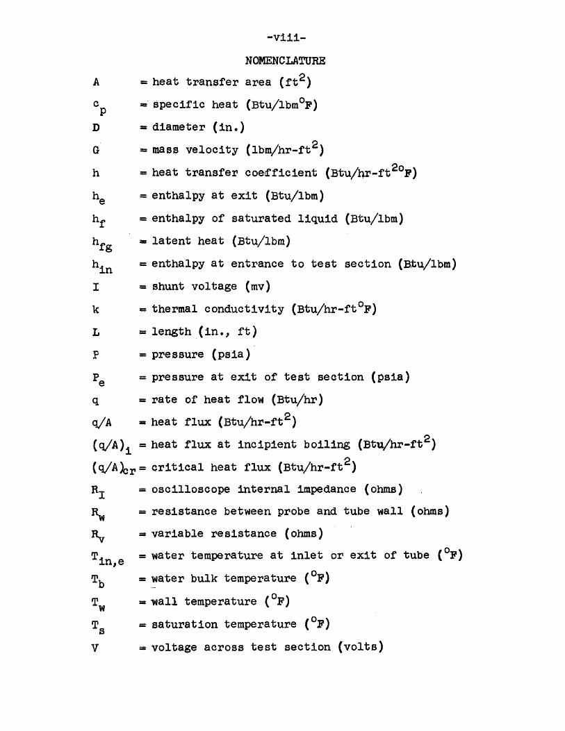
NOMENCLATURE

A heat transfer area (ft2)

c = specific heat (Btu/lbm0 F)

D diameter (in.)

G mass velocity (lbm/hr-ft2)

h = heat transfer coefficient (Btu/r-ft2OF)

he = enthalpy at exit (Btu/lbm)

h = enthalpy of saturated liquid (Btu/lbm)

h f = latent heat (Btu/lbm)

h = enthalpy at entrance to test section (Btu/lbm)

I= shunt voltage (mv)

k = thermal conductivity (Btu/hr-ft0 F)

L = length (in., ft)

P = pressure (psia)

Pe = pressure at exit of test section (psia)

q = rate of heat flow (Btu/hr)

q/A = heat flux (Btu/hr-ft2 )

(q/A ) = heat flux at incipient boiling (Btu/hr-ft 2 )

(q/A)cr= critical heat flux (Btu/hr-ft 2)

Ry I = oscilloscope internal impedance (ohms)

Rw = resistance between probe and tube wall (ohms)

Rv = variable resistance (ohms)

Tin,e = water temperature at inlet or exit of tube (OF)

Tb = water bulk temperature (OF)

Tw = mall temperature (OF)

T, 8 = saturation temperature (0F)

V = voltage across test section (volts)

-ix-

VB = battery voltage (volts)

VI = voltage across variable resistor (volts)

w = mass flow rate (lbm/hr)

x = quality

P= viscosity (lbm/hr-ft)

Flow Regime Designations

B = * =bubbly

BTS = = bubbly-to-slug wransition

S = 0 = slug

STA = 3 = first indication of slug-to-annular transition

STA = A = slug-to-annular transition

A = g = annular

WA = = wispy anrular

-1-

Chapter I

INTRODUCTION

1.1 Backpround of Problem

In recent years the interest in two-phase, gas-liquid

flow has dramatically expanded as is indicated by the tre-

mendous increase in the number of experiments and published

papers in this field. If one examines the literature, one

will find that a relatively large number of models have

been proposed for analyzing and correlating experimental

pressure-drop, heat-transfer, critical heat flux, and void-

fraction data. These models frequently depend on the flow

regimes (or flow patterns) which are geometric descriptions

of the distribution of the liquid and gas phases within a

channel. Gouse(l)* considers knowledge of the flow regime

to be as important as knowing whether the flow is laminar

or turbulent in single-phase flow.

Baker(2) showed that it was not practical to disregard

the flow regimes in devising a two-phase pressure-drop

correlation. Martinelli's (3) assumptions in his pressure-

drop correlations tend to limit them to annular flow,

Lavin and Young(4) propose boiling heat-transfer correla-

tions for refrigerants, which are dependent on the flow

regimes. Numerous models for the critical heat flux condi-

tion are based on the postulate of spray annular flow;

however, there are some analyses which assume that fog flow

is present.

*Numbers in parenthesis refer to References on p. 80.

-2-

It is apparent, then, that it is important to know

the flow regime if, one is to utilize an appropriate model;

however, direct relationships between flow regimes and-

6bservables, i.e., pressure drop, heat-transfer coeffi-

cient, critical heat flux, and void fraction have not been

clearly established.(5) Itistill appears, though, that

flow regime observations will be helpful in reducing the

complications of correlating the quantities of basic

interest.

A survey of the literature indicates that-flow regime

studies have almost always been conducted under adiabatic

conditions. However, exploratory studies have shown that

flow patterns are considerably altered when there is heat

addition, particularly in low pressure systems.(6)

Comprehensive flow regime maps have been prepared at

Dynatech and Harwell(9) for high pressure boiling

water systems. No similar study has been conducted at low

pressures (below 100 psia).

Low pressure systems are receiving increased atten-

tion, particularly in the nuclear reactor and desaliniza-

tion programs. In a recent study of critical heat fluxes

at low pressure, Lopina(lo) observed a pronounced effect

of inlet temperature. For constant geometry, flow rate,

and pressure level, the critical heat flux increased as

the inlet temperature increased. This effect, which is

contrary to what is observed at high pressures, appears to

be related to the flow regimes. The phenomenon of

-3-

upstream boiling burnout in uniformly heated channels also

appears to be related to flow regimes, in particular, the

slug flow regime.

1.2 Flow Regimes

There have been various descriptions of flow regimes

by different investigators, These classifications have

often been quite arbitrary, and are also complicated by the

fact that vertical and horizontal flows cause different

regimes. Baker(2) described no less than seven different

regimes in adiabatic two-phase, gas-liquid flow in horizon-

tal pipes. Vohr(ll) and Kepple and Tung(12) have presented

complete bibliographies on studies of adiabatic flow

patterns.

The flow regimes which may be encountered in flows in

tubes with vertical upflow can be described in the order of

increasing gas or vapor content. If very little gas or

vapor is involved, the flow will be characterized by isola-

ted vapor or gas bubbles dispersed rather uniformly in the

continuous liquid phase. This is known as "bubbly flow".

More bubbles appear with an increase of vapor ot gas until

the bubbles begin to touch one another and agglomerate.

As more bubbles agglomerate, the gas begins to flow in

long cylindrical, bullet-shaped bubbles, Between the

bubbles are slugs of liquid and hence "slug flow",

Further increase of the gas content destroys the stability

of the bubbles, producing "churn flow" or "semi-annular

flow" in which slugs of liquid separate adjacent gas

bubbles only temporarily. As the gas content continues to

increase, the liquid flows on the wall as an annular film

and the gas or vapor flows in the center of the tube. This

geometry is called "annular flow". "Fog flow" or "dispersed

flow" then follows where the gas or vapor phase occupies

the entire tube but small drops of liquid are dispersed

within it. This flow is also called "mist flow".

Other flow patterns which have been encountered are

"froth flow", "spray annular flow" and "wispy annular flow".

Froth flow is quite similar to bubbly flow except the

bubbles are so numerous that the flow has a frothy appear-

ance. Spray-annular flow is a combination of mist and annu-

lar flow. Some of the liquid flows in an annular film and

some flows as small droplets in the vapor core. Wispy annu-

lar is similar to spray annular except the flow in the core

consists of agglomerated liquid instead of small droplets.

There are very similar flow descriptions for horizontal

flow. However, stratification is sometimes encountered in

horizontal flow and several new regimes are introduced.

"Plug flow" is similar to slug flow except that the bubbles

move along the upper part of the channel or. pipe. In

"stratified flow" the liquid flows at the bottom, and gas or

vapor at the top of the pipe.

These regimes appear to be quite well defined. However,

for practical reasons it is desirable to minimize the

number of regimes. Gouse(1) suggests that there are only

four distinct flow patterns for vertical upflow: bubbly,

-5-

slug, annular, and mist; while all the others which have

been observed are merely transitions from one to another.

The above flows were described for adiabatic condi-

tions. In heated systems such clean geometric descriptions

of the flcw are not expected because of several character-

istics not encountered under adiabatic conditions. Some of

these 'characteristics are:

1) Vapor is continually formed along the tube. This

creates a volume flow rate which continuously increases

along the tube; thus the flow regimes would be expected to

be different in different sections of thetube.

2) Bubbles may be generated anCL disturb the flow

pattern.

In any case, the adiabatic flow regimes are a basis for

interpreting and classifying the flow regimes with heat

6ddition. The classification and both qualitative and semi-

quantitative description of the flow patterns observed in

this study are discussed in Section 2.3.3.

1.3 Flow Regime Detection

Numerous methods of studying flow regimes in heated

systems have been developed., High-speed still and movie

photography has been most popular. More exotic methods

which have been used include isokinetic flow sampling,

gamma or beta ray attenuation, and hot-wire anemometry.

Each of these methods has drawbacks. Either there is too

much data to analyze, as in the case of movies, or the

methods are Very complicated and expensive. The elegtri-

-6-

cal resistance probe which was 'developed by Solomon(13)

specifically for flow regime detection, is an inexpensive,

simple, and reliable device.

This probe measures the resistance between the center-

line of the fluid flow and the tube wall. A bridge of

liquid across the tube will cause a closed circuit, and

gas or steam across the tube will result in an open circuit.

Nassos(l4 ) and Haberstroh(15) have successfully used this

type of probe for adiabatic flow. Griffith(16 ) adapted

this probe for a high pressure boiling water system and

delineated the slug-to-annular transition. Dynatech(7)(8 )

has recently been using this technique to map boiling water

flow regimes at high pressures (500-1000 psia).

1.4 Scope of Research

A comprehensive study to examine boiling water flow

regimes in tubes of small diameter at pressures below 100

psia was undertaken. A resistance probe described in

detail in Section 2.2 was chosen as the primary means of

flow regime detection; however, a visual section was also

employed. The experimental program consisted of an inves-

tigation of the effects of velocity, inlet temperature,

exit pressure, quality, (heat flux), purity, length, diam-

eter, and orientation on the flow regimes. The first

phase of the study was devoted to probe development and

interpretation.

-7-

Chapter II

EXPERIMENTAL PROGRAM

2.1 Description of Apparatus

2.1.1 Hydraulic, System

The experimental facility used was the low-pressure

test loop located in the MIT Heat Transfer Laboratory. The

basc apparatus was designed and constructed in 1961:.(l7)

A schematic of the loop is presented in Fig. 1. The

pipings and fittings are made of brass and stainless steel

for corrosion resistance. Rayon reinforced rubber hose is

used where flexible connections are required. Distilled

water is circulated by a bronze, two-stage, regenerative

pump providing a discharge pressure of 260 psig at 3.6 gpm.

The pump is driven through a flexible coupling by a 3-hp

Allis-Chalmers induction motor. A Fulflo filter is in-

stalled at the pump inlet. Pressure fluctuations at the

outlet of the pump are damped out by means of a 2.5-gal

Greer accumulator charged with nitrogen to an initial

pressure of 40 psig. This accumulator contains a flexible

bladder-type separator which prevents the nitrogen from

being absorbed by the system water. After the accumulator,

the flow splits into the by-pass line and the test-section

line.

In the test-section line, fluid flows through a

Fischer-Porter flowrator followed by a preheater, thence

through a Hoke metering valve and the test section, after

which it merges with fluid from the by-pass line. The

-8-

flow then goes through the heat exchanger and returns to

the pump. The preheater consists of four Chromalox heaters

of approximately 6 kw each. Three of these are controlled

simply with "off-on" switches while the fourth can provide

a continuous range from 0 to 6 kw by means of a bank of

two variacs mounted on the test bench. Quick-action James-

bury ball valves are installed before the inlet to the

flowrator and after the exit from the test section. This

permits quick isolation of the test section to minimize

fluid loss when conducting burnout tests. The exit valve

is also used to adjust the test-section pressure.

Flow through the by-pass line is controlled by a ball

valve on each side of which there is a 300-psig pressure

gage. Pump operating pressure, and hence the pressure up-

stream of the test section, is controlled by this valve.

The heat exchanger is a counterflow type with system

water flowing in the inner tube and city water in the

outer annulus. Except at very high power levels, the heat

exchanger maintained a constant pump inlet temperature. A

Fulflo filter is installed on the city water line to

reduce scale formation in the exchanger.

The distilled water was de-ionized continuously,

except during contamination studies, by passing a portion

of the flow through four mixed-bed resin demineralizer

cartridges installed in a Barnstead- "Bantam" demineralizer

unit. A 4.7-gal degassing tank is provided with five elec-

trical heaters (3-200 vac and 2-110 vac). This tank also

-9-serves as a surge tank. A 15-gal stainless-steel storage

tank for filling the system is mounted directly above the

degassing tank and can be filled with distilled water from

standard 5-gal bottles with a small Hypro pump.

2.1.2 Power Supply

Test-section electrical power is provided by two

36-kw dc generators connected in series. Each generator is

rated at 12 volts and 3000 amperes. The power control con-

sole permits coarse or fine control from 0 to 24 volts. A

water-cooled shunt installed in parallel with the test sec-

tion protects the generators against the shock of the sudden

open circuit which occurs at burnout. Power is transmitted

from the main bus to the test section by water-cooled power

leads. In the present tests, the downstream or exit power

lead was at ground potential. Rubber hose connected both

inlet and exit chamber plenums to the main loop in order

to electrically isolate the test section. The exit of the

test section-was then separately grounded (see schematic

of test section, Fig. 2).

2.1.3 Instrumentation

All temperatures were measured by copper-constantan

thermocouples made from 30-gauge Leeds and Northrup duplex

wire. The test-section inlet temperature was measured by

a thermocouple directly in the fluid stream, upstream of

the Hoke metering valve. The thermocouple was introduced

at this location through a Conax fitting equipped with a

lava sealant.

-10-

All pressures were read on Bourdon-type gages located

as shown in Fig. 1. The test-section inlet and exit pressures

were measured with Helicoid 8-1/2 in. gages of 200 psig and

100 psig, respectively. Both are specified to an accuracy

of +0.25% of full scale.

A variety of metering tubes and floats, which could be

installe-d interchangeably in the basic Fischer-Porter flow-

meter housing, provided measurement of the test-section flow

from 1.5 to 4000 lbm/hr.

The voltage drop across the test section was read

directly on a Weston multiple-range dc voltmeter with a spec-

ified accuracy of + 1/2 percent. The current flow was

determined by using the Minneapolis-Honeywell, Brown recor-

der to measure the voltage drop across a calibrated shunt

(60.17 amp/mv) in series with the test section.

The details of the resistance probe are discussed in

Section 2.2. Polaroid cameras were used for the photo-

graphic study. The camera settings and procedures are dis-

cussed in Appendix B.

2.1.4 Operating Procedures

After the test section was installed, the loop and de-

gassing tank were filled with distilled water from the

supply tank. The water in the degassing tank was then

brought to a boil while the loop water was circulated with

the heat-exchanger coolant off. Degassing was accomplished

by by-passing a portion of the loop water into the top of

the vigorously boiling degassing tank. This was continued

-11-

until the temperature of the loop rose to approximately

1800f. A standard Winkler analysis described in Ref. 17

indicated that this method of degassing reduced the air

content to less than 0.1 cc air/liter. After completing

degassing, the loop water was adjusted, to the desired in-

let temperature and the desired pressures were set. A

pressure of from 210 psig to 260 psig was maintained at all

times on the upstream side of the Hoke metering valve to

prevent system-induced instabilities. The generators were

then started and allowed to warm up.

Nine burnout tests were made in order to have reliable

critical heat flux data for conditions similar to the planned

flow regime studies. This knowledge aided in avoiding burn-

out of the probe test sections. Power was applied to the test

section in small increments while maintaining a constant flow

rate and inlet temperature. The test-section flow rate,

shunt voltage (test-section current), inlet temperature, and

exit pressure were recorded for each voltage setting. The

critical or burnout heat flux was defined to be that heat flux

which caused physical f4ilure of the test section. After

commencing flow regime studies, it was seen that the area of

interest was usually far removed from (q/A)co. Consequently

no further burnout studies were made. Appendix A contains a

tabulation of the burnout points.

The same data were recorded for the flow regime runs.

A run consisted of taking data at a particular mass flow

rate for a given set of conditions, i.e. D, I/D, Ti, Pe.

-12-

As the power was increased, various responses on the oscil-

loscope indicated the type of flow (see Probe Interpretation,

Section 2.3). Water purity was checked by means of a

Barnstead Purity Meter (0.1 - 18 megohm-cm) or an Industrial

Instruments Solu-Bridge Meter (0 - 30 PPM NaCl).

2.2 Resistance Probe and Test Section

2.2,1 Principle of Operation

The resistance probe was used to determine the flow

regime at the exit of the test section. The probe is a wire

placed in the center of the tube as shown in Fig. 2. This

wire is covered by teflon sleeving except for the tip of the

wire. The circuit diagram for the probe is shown in Fig. 3a.

When there is a bridge of water across the tube at the test-

section exit, there is essentially a closed circuit between

the probe and the tube wall. This results in a maximum volt-

age across resistor RV which is measured by an oscillo-

scope. On the other hand, steam passing between the probe

and the wall resembles an open circuit giving a voltage

reading across RV near zero.

2.2.2 Probe Integration with Test Section

Two types of test sections were used for this study.

The first type was used for preliminary burnout studies.

The second type incorporated the resistance probe and a

sight section. The sight section was not always used

because the rubber gasket would not hold for exit pressures

above 40 psig, The heated sections were made of standard

-13-

304, stainless tubes. The burnout test sections and the first

probe test section had an 0.242-in. i.d. and 0.3125-in. o.d.

while the second probe test section had an i.d. of 0.094 in.

and o.d, of 0.120 in. The details of the two test sections

are shown in Fig. 2.,

In the burnout test section, 3/4-in, brass bushings

were silver-soldered to the stainless steel tube to form

the power connections upstream and downstream. A pressure

tap was installed in each exit bushing with a No. 80,

0.0135-in. diameter hole drilled through the tube wall.

The pressure tap was placed here rather than in the exit

plenum chamber because of the choking phenomera whereby the

plenum pressure is lower than the exit pressure.(l0)

The probe test section had pressure taps located at

both the inlet and exit. The exit section was modified to

include the probe and pyrex sight section. The inside

diameter of the glass tubing was equal to the outside diam-

eter of the test section. This caused a slight expansion

at the entrance to the visual section.

The brass supporting structure for the probe, pressure

tap, and sight section also served as the exit power connec-

tion. The pressure tap is similar to the previous one

described.

The probe was fabricated from 0.035-in, diameter temp-

ered stainless-steel spring wire for the 0.242-in, diameter

tube and from 0.015-in, wire for the 0.094-in, diameter

tube. Teflon spaghetti was slipped over this wire and

-14-

stretched until the teflon set snugly on the wire. The

final probe diameters were 0.060 in. and 0.031 in. Even the

small diameter probe had adequate stiffness to prevent vi-

bration which could create spurious signals.

The straight probe was pushed into the test section

from the packing gland side until it touched the opposite

wall. The tip was then carefully bent and the teflon was

forced around the wire until only a 1/4 in. of probe tip was

bare.

The teflon acts as an insulation between the probe and

the tube wall. More important, since teflon is not wetted

by water, there is no chance of a short-circuit between the

exposed end of the wire and the tube wall. The drying time

of the teflon after passage of a slug of liquid is extremely

short, less than 10-3 seconds as observed with an oscillo-

scope.(15)

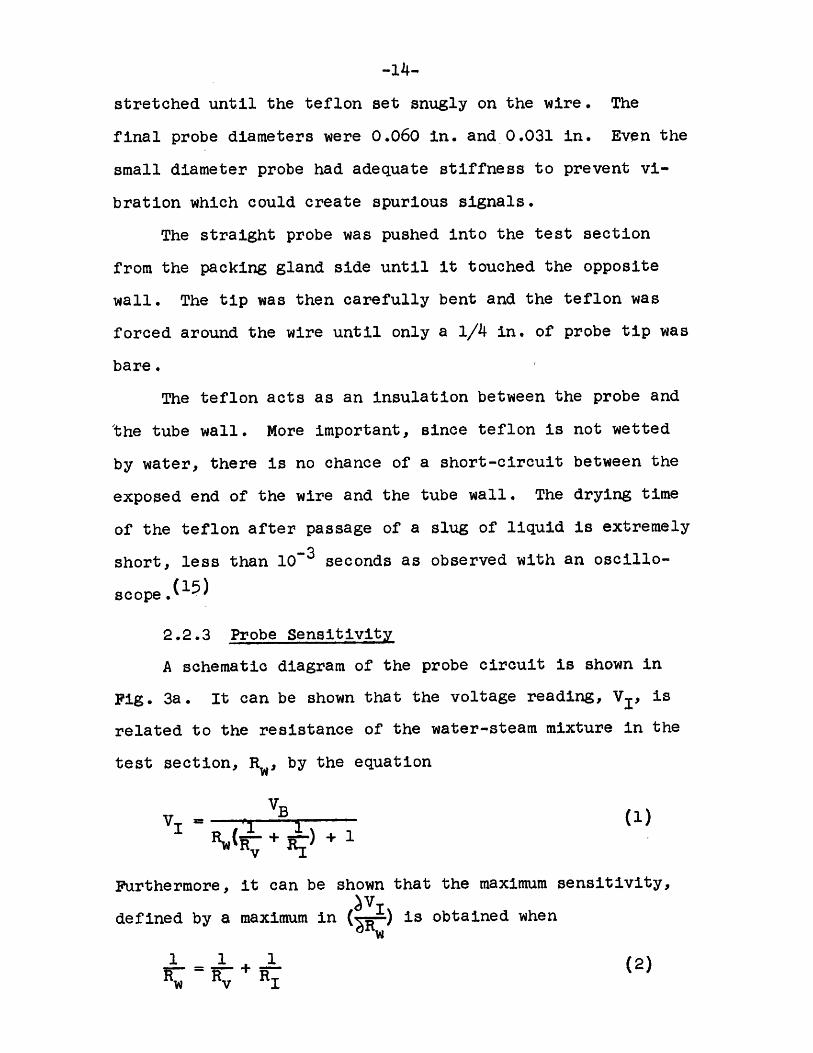
2.2.3 Probe Sensitivit

A schematic diagram of the probe circuit is shown in

Fig. 3a. It can be shown that the voltage reading, VI, is

related to the resistance of the water-steam mixture in the

test section, R., by the equation

V+ )B ()Rw(1 + -)+ 1

Furthermore, it can be shown that the maximum sensitivity,

defined by a maximum in ( I) is obtained whenRw

1 1 (2)Rw Rv RI

-15-

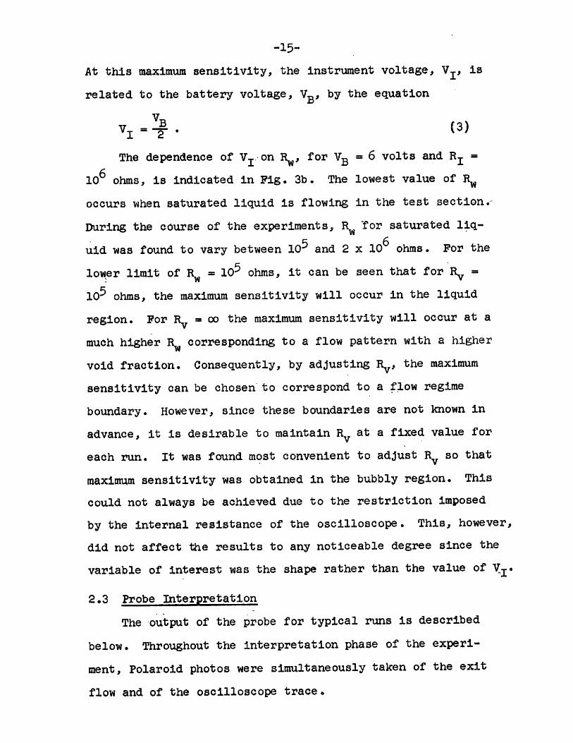
At this maximum sensitivity, the instrument voltage, V1, is

related to the battery voltage, VB, by the equation

V VB (3)

The dependence of V ton Rw, for VB = 6 volts and R=

106 ohms, is indicated in Fig. 3b. The lowest value of Rw

occurs when saturated liquid is flowing in the test section.-

During the course of the experiments, R, "for saturated liq-

uid was found to vary between 105 and 2 x 106 ohms. For the

lower limit of Rw = 105 ohms, it can be seen that forR =

105 ohms, the maximum sensitivity will occur in the liquid

region. For Rv = co the maximum sensitivity will occur at a

much higher R. corresponding to a flow pattern with a higher

void fraction. Consequently, by adjusting Rv, the maximum

sensitivity can be chosen to correspond to a flow regime

boundary. However, since these boundaries are not known in

advance, it is desirable to maintain Rv at a fixed value for

each run. It was found most convenient to adjust Rv so that

maximum sensitivity was obtained in the bubbly region. This

could not always be achieved due to the restriction imposed

by the internal resistance of the oscilloscope. This, however,

did not affect the results to any noticeable degree since the

variable of interest was the shape rather than the value of .

2.3 Probe Interpretation

The -output of the probe for typical runs is described

below. Throughout the interpretation phase of the experi-

ment, Polaroid photos were simultaneously taken of the exit

flow and of the oscilloscope trace.

-16-

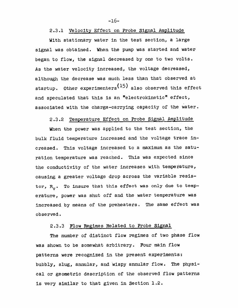
2.3.1 Velocity Effect on Probe Signal Amplitude

With stationary water in the test section, a large

signal was obtained. When the pump was started and water

began to flow, the signal decreased by one to two volts.

As the water velocity increased, the voltage decreased,

although the decrease was much less than that observed at

startup. Other experimenters(15) also observed this effect

and speculated that this is an "electrokinetic" effect,

associated with the charge-carrying capacity of the water.

2.3.2 Temperature Effect on Probe Signal Amplitude

When the power was applied to the test section, the

bulk fluid temperature increased and the voltage trace in-

creased. This voltage increased to a maximum as the satu-

ration temperature was reached. This was expected since

the conductivity of the water increases with temperature,

causing a greater voltage drop across the variable resis-

tor, Rv* To insure that this effect was only due to temp-

erature, power was shut off and the water temperature was

increased by means of the preheaters. The same effect was

observed.

2.3.3 Flow Regimes Related to Probe Signal

The number of distinct flow regimes of two phase flow

was shown to be somewhat arbitrary. Four main flow

patterns were recognized in the present experiments:

bubbly, slug, annular, and wispy annular flow. The physi-

cal or geometric description of the observed flow patterns

is very similar to that given in Section 1.2.

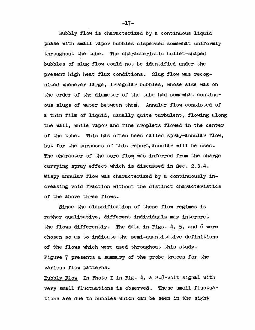
-17-

Bubbly flow is characterized by a continuous liquid

phase with small vapor bubbles dispersed somewhat uniformly

throughout the tube. The characteristic bullet-shaped

bubbles of slug flow could not be identified under the

present high heat flux conditions. Slug flow was recog-

nized whenever large, irregular bubbles, whose size was on

the order of the diameter of the tube had somewhat continu-

ous slugs of water between then!. Annular flow consisted of

a thin film of liquid, usually quite turbulent, flowing along

the wall, while vapor and fine droplets flowed in the center

of the tube. This has often been called spray-annular flow,

but for the purposes of this reportannular will be used.

The character of the core flow was inferred from the charge

carrying spray effect which is discussed in Sec. 2.3.4.

Wispy annular flow was characterized by a continuously in-

creasing void fraction without the distinct characteristics

of the above three flows.

Since the classification of these flow regimes is

rather qualitative, different individuals may interpret

the flows differently. The data in Figs. 4, 5, and 6 were

chosen so as to indicate the semi-quantitative definitions

of the flows which were used throughout this study.

Figure 7 presents a summary of the probe traces for the

various flow patterns.

Bubbly Flow In Photo I in Fig. 4, a 2.8-volt signal with

very small fluctuations is observed. These small fluctua-

tions are due to bubbles which can be seen in the sight

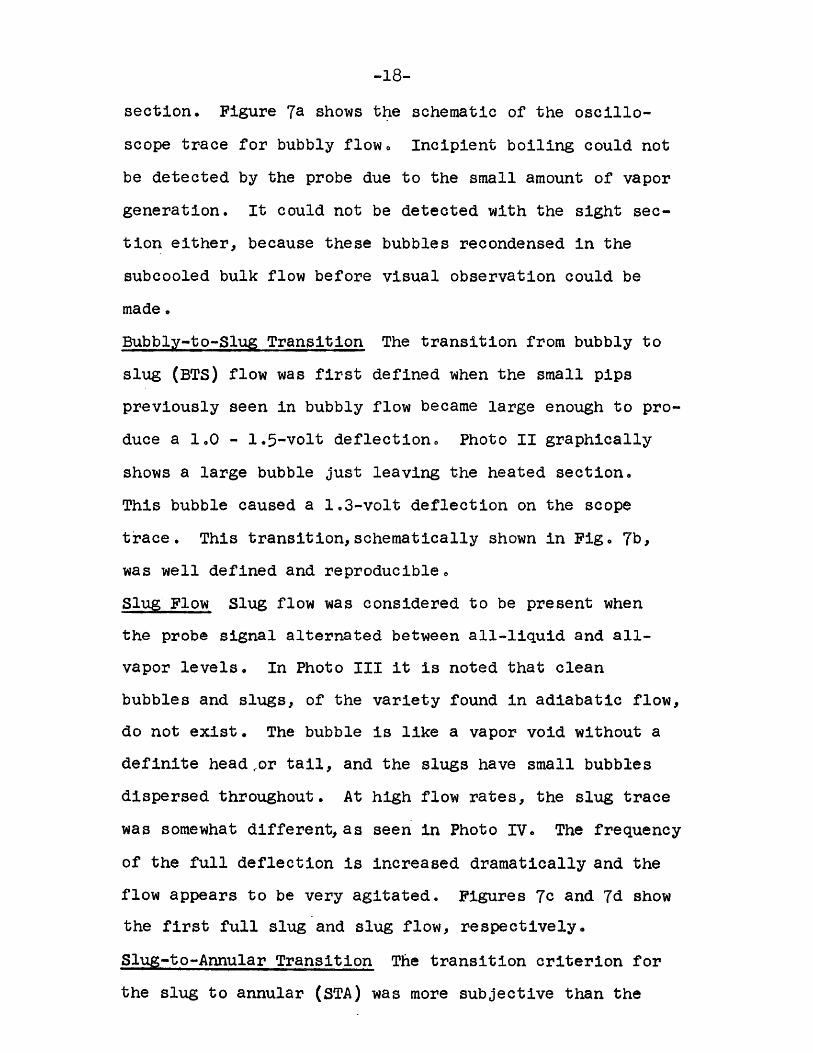
-18-

section. Figure 7a shows the schematic of the oscillo-

scope trace for bubbly flow, Incipient boiling could not

be detected by the probe due to the small amount of vapor

generation. It could not be detected with the sight sec-

tion either, because these bubbles recondensed in the

subcooled bulk flow before visual observation could be

made.

Bubbly-to-Slug Transition The transition from bubbly to

slug (BTS) flow was first defined when the small pips

previously seen in bubbly flow became large enough to pro-

duce a 1.0 - 1.5-volt deflection. Photo II graphically

shows a large bubble just leaving the heated section.

This bubble caused a 1.3-volt deflection on the scope

trace. This transitionschematically shown in Fig. 7b,

was well defined and reproducible.

Slug-Flow Slug flow was considered to be present when

the probe signal alternated between all-liquid and all-

vapor levels. In Photo III it is noted that clean

bubbles and slugs, of the variety found in adiabatic flow,

do not exist. The bubble is like a vapor void without a

definite head, or tail, and the slugs have small bubbles

dispersed throughout. At high flow rates, the slug trace

was somewhat differentas seen in Photo IV. The frequency

of the full deflection is increased dramatically and the

flow appears to be very agitated. Figures 7c and 7d show

the first full slug and slug flow, respectively.

Slug-to-Annular Transition The transition criterion for

the slug to annular (STA) was more subjective than the

-19-

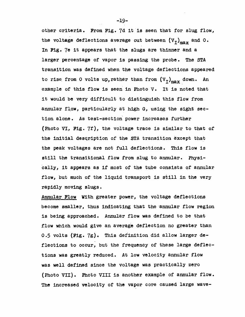
other criteria. From Fig. 7d it is seen that for slug flow,

the voltage deflections average out between (VI)max and 0.

In Fig. 7e it appears that the slugs are thinner and a

larger percentage of vapor is passing the probe. The STA

transition was defined when the voltage deflections appeared

to rise, from 0 volts uprather than from (VI)max down. An

example of this flow is seen in Photo V. It is noted that

it would be very difficult to distinguish this flow from

annular flow, particularly at high G, using the sight sec-

tion alone. As test-section power increases further

(Photo VI, Fig. 7f), the voltage trace is similar to that of

the initial desqription of the STA transition except thatthe peak voltages are not full deflections. This flow is

still the transitional flow from slug to annular. Physi-

cally, it appears as if most of the tube consists of annular

flow, but much of the liquid transport is still in the very

rapidly moving slugs.

Annular Flow With greater power, the voltage deflections

become smaller, thus indicating that the annular flow region

is being approached. Annular flow was defined to be that

flow which would give an average deflection no greater than

0.5 volts (Fig. 7g), This definition did allow larger de-

flections to occur, but the frequency of these large deflec-

tions was greatly reduced. At low velocity annular flow

was well defined since the voltage was practically zero

(Photo VII). Photo VIII is another example of annular flow.

The increased velocity of the vapor core caused large wave-

-20-

like motions on the surface of the annular film. These

waves appeared as large deflections on the oscilloscope.

As G was increased, these waves increased in frequency and

the film had a milky appearance, probably due to the in-

creased entrainment and deposition of droplets. Very

little could have been said about the interior flow, i.e.

waves,if only photography had been used in this study.

Wispy Annular Under certain conditions, i.e. Tin = 2000F,

P = 20-30 psia, G = 1.6 - 2.0 x 106 lbm/hr-ft2 , a varia-

tion of the above flow regimes was noted. As power was

increased beyond bubbly flow, a strong bubbly trace

travelled downward from (VI)max to 0 volts. Slug flow did

not appear and in its place was a flow which can be called

wispy annular 9 or froth(8 I. The behavior of the trace

is schematically shown in Figs. 7h, Ti, and 7j and in the

corresponding Photos IX, X, and XI. As the void fraction

is increased, the resistance between probe and wall

becomes greater until annular flow is reached. It would

be possible to describe many flow patterns in this high-

velocity transition between bubbly and annular flow.

Froth flow would probably be a more appropriate descrip-

tion of the beginning of this transition, while wispy annu-

lar could describe the latter part of the transition.

Since the probe indicated that the transition was quite

homogeneous throughout, it appears that a single classi-

fication is adequate.

-21-

2.3.4 Charge Carrying Spray Effect

Photo XII again shows annular flow, but the oscillo-

scope trace is radically different in that negative traces

up to one volt are seen. This type of trace was not ob-

served in high pressure studies(16,8 ) and initially caused

quite a bit of trouble in interpretation. With the probe

circuit battery removed and the oscilloscope connected

directly across the probe, a fluctuating negative voltage

was still observed. The magnitude and frequency of this

fluctuation increased as the flow rate was increased, even

though no voltage source was present. A possible pickup

effect on the probe from the voltage across the test tube

was discounted because the generator output voltage did

not have such large fluctuations.

The explanation of this negative voltage effect is

believed to be as follows. As annular flow is approached,

small droplets of water are torn away from the liquid

film and are transported as a spray in the core. By some

physical effect these droplets become negatively charged

upon detaching from the bulk flow, thus leaving the film

positively charged. The droplets travel down the tube and

rejoin the film and lose their charge, escape through the

exit and lose their charge in the loop, or deposit their

charge on the probe. This last possibility appears to be

the source of the negative voltage observed on the scope.

Professor D. P. Keily(l8) has observed such effects with

aerosol-type flows and indicated that voltages up to

-22-

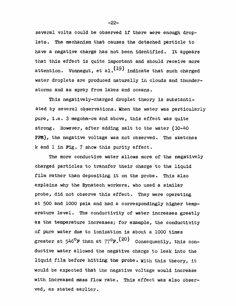
several volts could be observed if there were enough drop-

lets. The mechanism that causes the detached particle to

have a negative charge has not been identified. It appears

that this effect is quite important and should receive more

attention. Vonnegut, et al.(19) indicate that such charged

water droplets are produced naturally in clouds and thunder-

storms and as spray from lakes and oceans.

This negatively-charged droplet theory is substanti.-

ated by several observations. When the water was particularly

pure, i.e. 3 megohm-cm and above, this effect was quite

strong. However, after adding salt to the water (30-40

PPM), the negative voltage was not observed. The sketches

k and 1 in Fig. 7 show this purity effect.

The more conductive water allows more of the negatively

charged particles to transfer their charge to the liquid

film rather than depositing it on the probe. This also

explains why the Dynatech workers, who used a similar

probe, did not observe this effect. They were operating

at 500 and 1000 psia and had a correspondingly higher temp-

erature level. The conductivity of water increases greatly

as the temperature increases; for example, the conductivity

of pure water due to ionization is about a 1000 times

o o(20)greater at 5460F than at T70F.(2) Consequently, this con-

ductive water allowed the negative charge to leak into the

liquid film before hitting the probe. With this theory, it

would be expected that the negative voltage would increase

with increased mass flow rate. This effect was also obser-

ved, as stated earlier.

-23-

Several methods were attempted to eliminate this effect

electronically by using a higher battery voltage, and by

using an ac high-frequency voltage source. The first

method reduced the relative voltage of the effect but did

not eliminate it. By means of filter circuits and high

frequency ac, it was hoped to eliminate the spurious nega-

tive charge and retain only the desired signals. However,

the filters and bias circuits also removed the desired

fluctuations. With experience it was found that proper

interpretations of the flows could be made even though the

negative voltage was present.

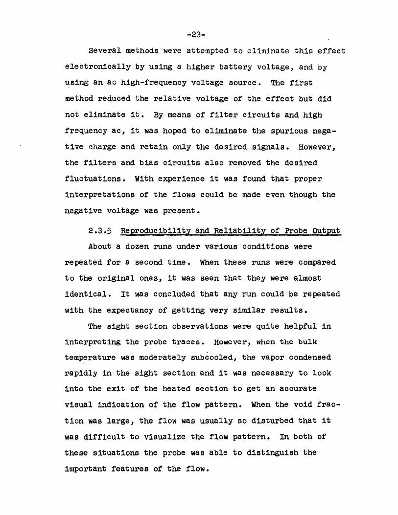
2.3.5 Reproducibility and Reliability of Probe Output

About a dozen runs under various conditions were

repeated for a second time. When these runs were compared

to the original ones, it was seen that they were almost

identical. It was concluded that any run could be repeated

with the expectancy of getting very similar results.

The sight section observations were quite helpful in

interpreting the probe traces. However, when the bulk

temperature was moderately subcooled, the vapor condensed

rapidly in the sight section and it was necessary to look

into the exit of the heated section to get an accurate

visual indication of the flow pattern. When the void frac-

tion was large, the flow was usually so disturbed that it

was difficult to visualize the flow pattern. In both of

these situations the probe was able to distinguish the

important features of the flow.

'~)-C. U-

2.4 Test Program

After the probe calibration and interpretation runs

were completed, the actual flow-regime investigations were

started. The following table lists all the sets of runs

completed in this experimental program.

All the data are presented on flow regime maps. The

coordinates of mass velocity (G) and mass quality (x) were

chosen because it appeared that they were best suited in

presenting the various effects studied. In addition, they

are usually the most convenient for engineering applica-

tions. Researchers in adiabatic two-phase flow frequently

make use of volume flow rate and volume quality coordinates.

They could not be used for this study since noneqiuilibrium

effects dominated and these quantities cannot be calculated.

Several runs are also presented in terms of heat flux and

quality to demonstrate a particular effect.

Due to the manner in which the loop operates, it was

difficult to control the exit pressure very accurately.

Consequently, pressure comparisons were made at low

pressures where the exit pressure varied from 20-35 psia

and at high pressures between 90-100 psia. These small

pressure differences did not affect the results to any

appreciable degree in comparison to the effects due to the

large difference between high and low pressures.

2.5 Data Reduction

All data were reduced by machine computation. The IBM

7094 Computer at the MIT Computation Center was used. The

Table 1

O x 10-6ihm

ft g-hr.0.4-2.00.8-2.00.2-2.40.2-2.40.2-2.40.4-2.4

0.4-2.40.2-1.6(B.O.)0.2-2.4-0.4-2.0

0.4-2.4

0.4-2.4

Water PurityMegohm-cm( or )

PPM

9 PPM0.48 mesohm-cm

2.5^2

Water waschecked atleast threetimes inevery setand found tobe between

-3.0 mego-

All previous sets were horizontal, No. 13 is vertical

13 60 0.242 100 .-30

set

12

34

56

78

9101112

D(in.)0.2420.242

0.2420.2420.2420.242

0.242

0.2420.2420.242

0.094

0.094

60k6060606060606030

90906060

T i0F

100100100

150200100200100100100100200

(12sia)-

'--20-30-20-30--20-30-20-'0

-20-30-100'-100-^ 30'-'30

-100-30-30

8

91011121314

1516

171819

200.*2-2.*0

-26-

program is described in Appendix C. The heat flux was

determined by the formula

(q/A) = El (4)

The equilibrium exit quality is given by

X q/w + h i - h5)= h (5)hfg

-27-

Chapter III

PRESENTATION AND DISCUSSION OF RESULTS

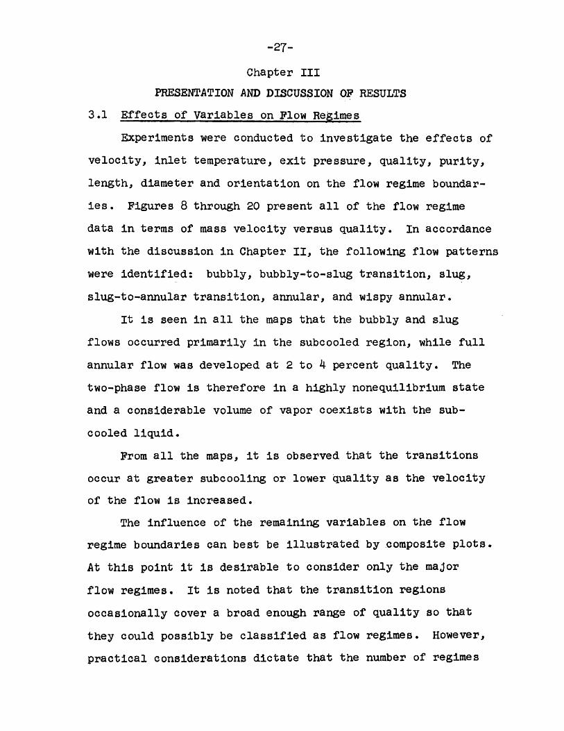
3.1 Effects of Variables on Flow Regimes

Experiments were conducted to investigate the effects of

velocity, inlet temperature, exit pressure, quality, purity,

length, diameter and orientation on the flow regime boundar-

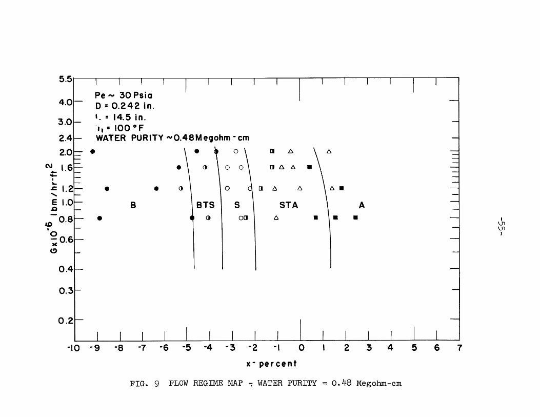
ies. Figures 8 through 20 present all of the flow regime

data in terms of mass velocity versus quality. In accordance

with the discussion in Chapter II, the following flow patterns

were identified: bubbly, bubbly-to-slug transition, slug,

slug-to-annular transition, annular, and wispy annular.

It is seen in all the maps that the bubbly and slug

flows occurred primarily in the subcooled region, while full

annular flow was developed at 2 to 4 percent quality. The

two-phase flow is therefore in a highly nonequilibrium state

and a considerable volume of vapor coexists with the sub-

cooled liquid.

From all the maps, it is observed that the transitions

occur at greater subcooling or lower quality as the velocity

of the flow is increased.

The influence of the remaining variables on the flow

regime boundaries can best be illustrated by composite plots.

At this point it is desirable to consider only the major

flow regimes. It is noted that the transition regions

occasionally cover a broad enough range of quality so that

they could possibly be classified as flow regimes. However,

practical considerations dictate that the number of regimes

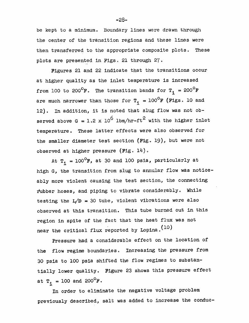
be kept to a minimum. Boundary lines were drawn through

the center of the transition regions and these lines were

then transferred to the appropriate composite plots. These

plots are presented in Figs. 21 through 27.

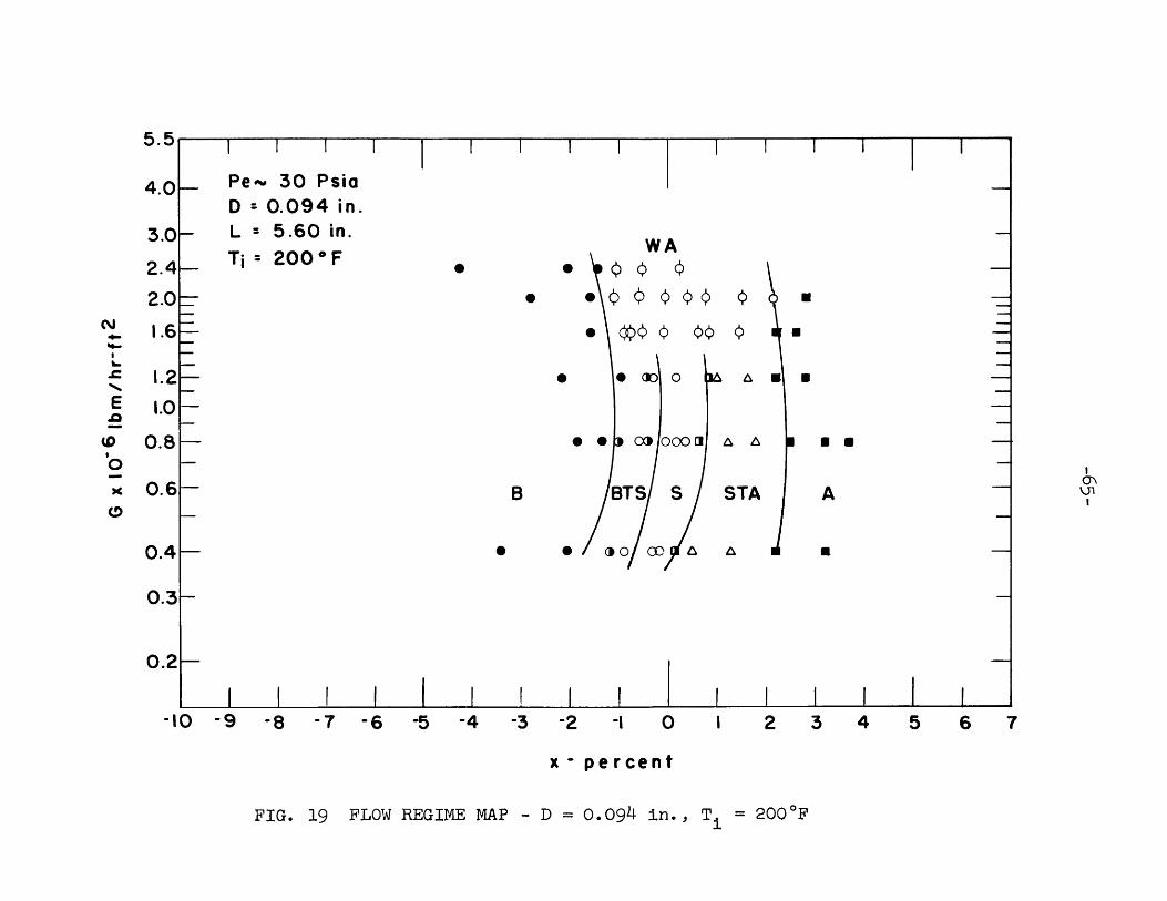
Figures 21 and 22 indicate that the transitions occur

at higher quality as the inlet temperature is increased

from 100 to 2000F. The transition bands for Ti = 2000F

are much narrower than those for Ti = 1000F (Figs. 10 and

12). In addition, it is noted that slug flow was not ob-

served above G = 1.2 x 106 lbm/hr-ft2 with the higher inlet

temperature. These latter effects were also observed for

the smaller diameter test section (Fig. 19), but were not

observed at higher pressure (Fig. 14).

At Ti = 100 0F, at 30 and 100 psia, particularly at

high G, the transition from slug to annular flow was notice-

ably more violent causing the test section, the connecting

zubber hoses, and piping to vibrate considerably. While

testing the L/D = 30 tube, violent vibrations were also

observed at this transition. This tube burned out in this

region in spite of the fact that the heat flux was not

near the critical flux reported by Lopina.(0)

Pressure had a considerable effect on the location of

the flow regime boundaries. Increasing the pressure from

30 psia to 100 psia shifted the flow regimes to substan-

tially lower quality. Figure 23 shows this pressure effect

at T = 100 and 2000F.

In order to eliminate the negative voltage problem

previously described, salt was added to increase the conduc-

-29-

tivity of the water. The effect of this dissolved impurity

on the flow regimes is illustrated in Fig. 24. The BTS

transition for very pure water (2.5 megohm-cm) occurs at

slightly higher quality than the transition for the 1 and

9 PPM water. There was no discernible effect in the STA

transition. Conductivity variations between 1 and 3

megohm-cm produced no noticeable shift in the flow regimes.

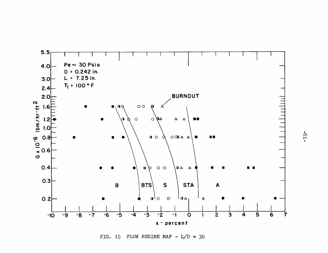
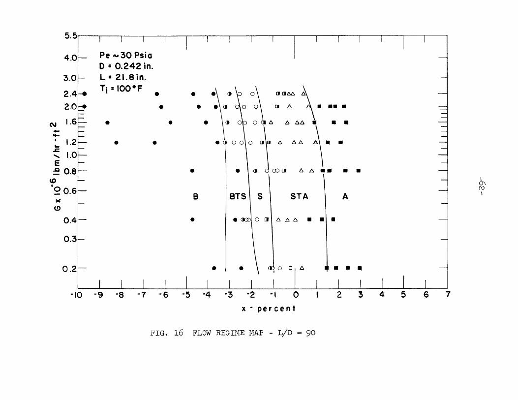
Length-to-diameter ratios of 30, 60 and 90 were

examined. From Fig. 25, it is seen that the flow regimes

are quite similar, although for an L/D = 30 the transitions

are at slightly lower quality.

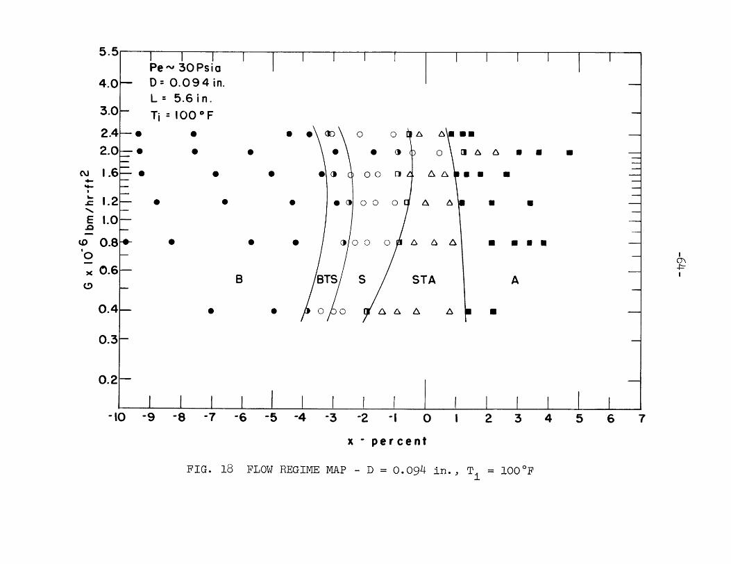
For the same Ti there was no discernable difference in

the flow regime maps for the two diameters (Fig. 26).

In Fig. 27 it is seen that the transition lines have

the same general shape for the horizontal and vertical test

sections. There is a slight shift to lower quality for the

vertical section. At velocities below 0.4 x 106 lbm/hr-ft2

slight stratification was visually observed for the bubbly

and BTS transitions. Since the vertical test section

showed only a minor flow regime variation from the horizon-

tal section, it is evident that this stratification did not

affect the probe output at the particular position, i.e.

center, that the probe was in. A modification of the

probe design, whereby the probe could be moved radially

across the tube during operation, would allow examination

of the flow very close to the walls and thus would detect

any stratification.

-30-

3.2 Explanation of Results

The various effects noted above appear to be very

closely related to incipient boiling, heat flux, and tur-

bulence of the flow. To explain this relationship, the

requirements for the transition to slug flow are first

examined.

Radovich and Moissis(21) have shown that the frequency

of bubble collisions is very high in two-phase bubbly flow.

A relatively small number of these collisions results in

coalescence. As more bubbles coalesce, the bubbles

increase in size to such an extent that slug flow is obser-

ved. The time that it takes to cause the first identifiable

existence of slug flow has been called the agglomeration

time. The agglomeration time is thus determined by the

collision frequency and the probability of coalescence per

collision. The latter quantity was found to be strongly

dependent on the purity of the liquid. Since the liquid

used in this study was maintained at relatively constant

purity for most of the experiments, the agglomeration time

depended primarily on the collision frequency. A decrease

in the agglomeration time would mean a shifting of the BTS

transition to lower quality. This could be accomplished

by increasing the number of bubbles and by causing greater

turbulence in the flow.

The requirements for incipient nucleation in a forced-

convection surface-boiling system have been considered in

detail by Bergles and Rohsenow,(22) When their correlation

-31-

was applied to the present conditions (Appendix D), it was

found that incipient boiling occurred at greater subcooling

as G increased, Ti decreased, and Pe increased. Further-

more, it can be seen from Figs. 28 to 31 that the heat flux

level increases as G increases, Ti decreases.,-and Pe

increases. As the heat flux increases there is an increase

in the bubble population. Boring(23) has concluded that

as heat flux and velocity increase, there is an increase

in the subcooling at which detatchment of the bubbles from

the heated surface occurs. This is due primarily to a

general increase in turbulent mixing under these conditions.

This enhanced mixing should promote the agglomeration of

bubbles.

Thus, on the basis of incipient boiling, heat flux,

and mixing considerations, one would expect a shift in the

BTS transition to greater subcooling as G increases, Ti

decreases, and Pe increases. These trends are observed in

the present data, as was discussed in the preceding section.

Since the heat flux level increases as the tube length

decreases, the shifting of the BTS transition to greater sub-

cooling as length is decreased is also accounted for.

Regarding the other transitions, it is reasonable to

expect that if the BTS transition occurs at lower quality,

the STA transition should also occur at lower quality. In

particular, the increased bubble agitation at the higher

heat fluxes would be expected to break up the slugs, thereby

promoting annular flow.

-32-

The limited occurrance of wispy annular flow can be

related to the above arguments. It is recalled that this

regime occurred only for high inlet temperature and low

pressure. Under these conditions the heat flux level is

low and there are fewer bubbles and also less tendency for

the bubbles to agglomerate into slugs, The core flow

remains bubbly or forthy in appearance until the void

fraction is so high that the spray annular configuration

is reached. In general the wispy annular regime is only

observed at high velocity where the short transit times are

less condusive to formation of slug flow.

At this point it is worth mentioning that Radovcich

and Moissis predicted that the BTS transition would be much

more rapid for pure water. As discussed in the preceding

section, the present tests indicated that this transition

for the demineralized water occurred at about the same

quality as that for the water with dissolved salt.

Their observation was for adiabatic flow; thus, with heat

addition the other mechanisms appear to overshadow the

impurity effect.

3.3 Interpretation of Critical Heat Flux Data by Means of

Flow Regimes

The present flow regime observations should be useful

in interpreting heat transfer and pressure drop data for

boiling water at low pressures. As an example of the

application of the present data, one of the important

effects in bulk boiling burnout will be considered.

-33-

Recent studies of bulk boiling at low pressure have

confirmed that the critical condition coincides with the

disappearance of the liquid film from the heated surface .(24)

The film can be depleted by evaporation and entrainment, or

it can be disrupted by bubble nucleation. In addition to

these local effects it appears that unstable upstream flow

patterns can produce a disruption of the annular film

further downstream.

LopinalO) found that the burnout heat flux increased

as the inlet temperature increased. Typical data illustra-

ting this effect are plotted in Fig. 33. The flow regimes

for these conditions are superimposed on the operating lines.

First consider operation at high inlet temperature as

shown in Fig. 33. The majority of the tube is in annular

flow with only moderate increases in hpat flux. The slug

flow region of the tube becomes increasingly violent, but

also moves toward the inlet, as the heat flux is increased.

This unstable slug flow region should have little effect on

the critical heat flux, which for these flow conditions is

probably caused by nucleation-induced breakup of the film.

Now, as the inlet temperature is decreased, the slug flow

region remains in closer proximity to the exit of the tube

and the disturbance created within this region would be

expected to propagate downstream and affect the film at its

thinnest poiht, which is at the exit of the tube. A

significant reduction in the critical heat flux is thus

-34-

observed as the inlet temperature is increased.

With short test sections the operating region will lie

in the vicinity of zero quality. In this case the unstable

slug flow regime is at the exit to the test section and

relatively low burnout fluxes, noted in the present L/D =

30 tests, for example, would be expected.

-35-*

Chapter IV

CONCLUSIONS

4.1 Cohclusions

The conclusions of this investigation can be summarized

as follows:

1) The electrical resistance probe is exceptionally

well suited for flow regime studies. It is simple, inexpen-

sive, and provides reliable and consistent results. For

low pressure studies, where nonequilibrium effects dominate,.

the probe is more reliable than an exit sight section.

2) The interesting phenomenon of the spray particles

carrying a negative charge has been observed. The cause of

this effect is not yet known, but various researchers are

investigating the problem.. Although it influenced the

probe output under certain conditions, it did not inhibit the

flow regime analysis.

3) Flow regime observations were made for low pressure

water over a wide range of flow conditions. The major flow

regimes observed were bubbly, slug, annular, and wispy annu-

lar flow. The flow regime maps show that bubbly, transition

to slug, slug, and transition to annular flow occur in the

subcooled region under nonequilibrium conditions while a

fully developed annular flow exists by the time 2-4 percent

quality is reached.

4) The observed effects of the parameters on the

flow regimes are summarized in the table below.

Table II

Parameter

Mass Velocity

Inlet Temper-ature

Pressure

Purity

Length

Diameter

Orientation

Direction ofChange inParameter

Increase

Increase

Increase

Decreased

Increased,

Decreased

Horizontal tovertical,

Direction of Shift ofFlow Regime Boundaries

towards greater subcooling

towards less subcooling

towards greater subcooling

negligible change

slight change towards less sub-cooling

negligible change

negligible change

5) The influence of velocity, temperature, pressure and

length on the flow regime boundaries can be explained in terms

of incipient boiling, heat flux, and turbulent mixing consid-

erations.

6) The present observations were applied to bulk boil-

ing burnout data. It was found that the effect of inlet temp-

erature on burnout can be related to unstable upstream flow

patterns.

APPENDIX

-38-

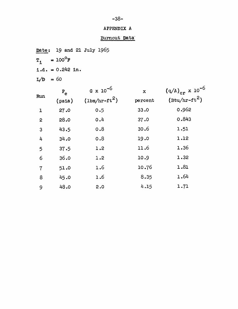
APPENDIX A

Burnout Data'

Date: 19 and 21 July 1965

T = lo0"F

i.d. = 0.242 in.

L/D = 60

G x 106

(lbm/hr-ft 2 )

0.5

0.4

o.8

o.8

1.2

1.2

1.6

1.6

2.0

x

percent

33.0

37.0

30.6

19.0

11.6

10.9

10.76

8.35

4.15

(q/A)cr 10-6

(Btu/hr-ft 2 )

0.962

0.843

1.51

1.12

1.36

1032

1.81

1.64

1.71

Run

1

2

3

4

5

6

7

8

9

Pe

(psia)

27.0

28.0

43.5

34.0

37.5

36.0

51.0

45.0

48.0

-39-

APPENDIX B

Photographic Procedures

For the photographic study, simultaneous pictures were

taken of the oscilloscope trace and of the exit flow in the

glass sight section. This was accomplished by shooting both

pictures manually at the same time at the desired flow

conditions.

The Polaroid Oscilloscope Camera for the Hewlett-Packard

Company Model 130B/BR Oscilloscope was used. The film was

Polaroid ASA 3000 film and the camera settings were f 2.8

and speed of 1/30 sec.

The sight section was normally illuminated by a

General Radio Co. Strobotac. The Strobotac was always off

when actually taking photos.

For the sight section photos, Polaroid ASA 200 Film was

used in order to obtain better quality pictures. A General

Radio Co. Type 1530-A Microflash was used to illuminate the

exit test section. The 2-microsecond light pulse effectively

stopped the motion of the flow in the sight section. Various

backgrounds for the sight section were tried with black

velvet giving the best results. The Polaroid camera was

mounted on a tripod and the +2 and +4 Polaroid close-up

lenses were used. The camera settings were f.8 and 1/30 sec.

Below is a sketch of the lighting setup viewed from

above. The microflash was approximately 12 inches below the

test section and was inclined so that the light was pointed

directly at the sight section,

--40-

-41-

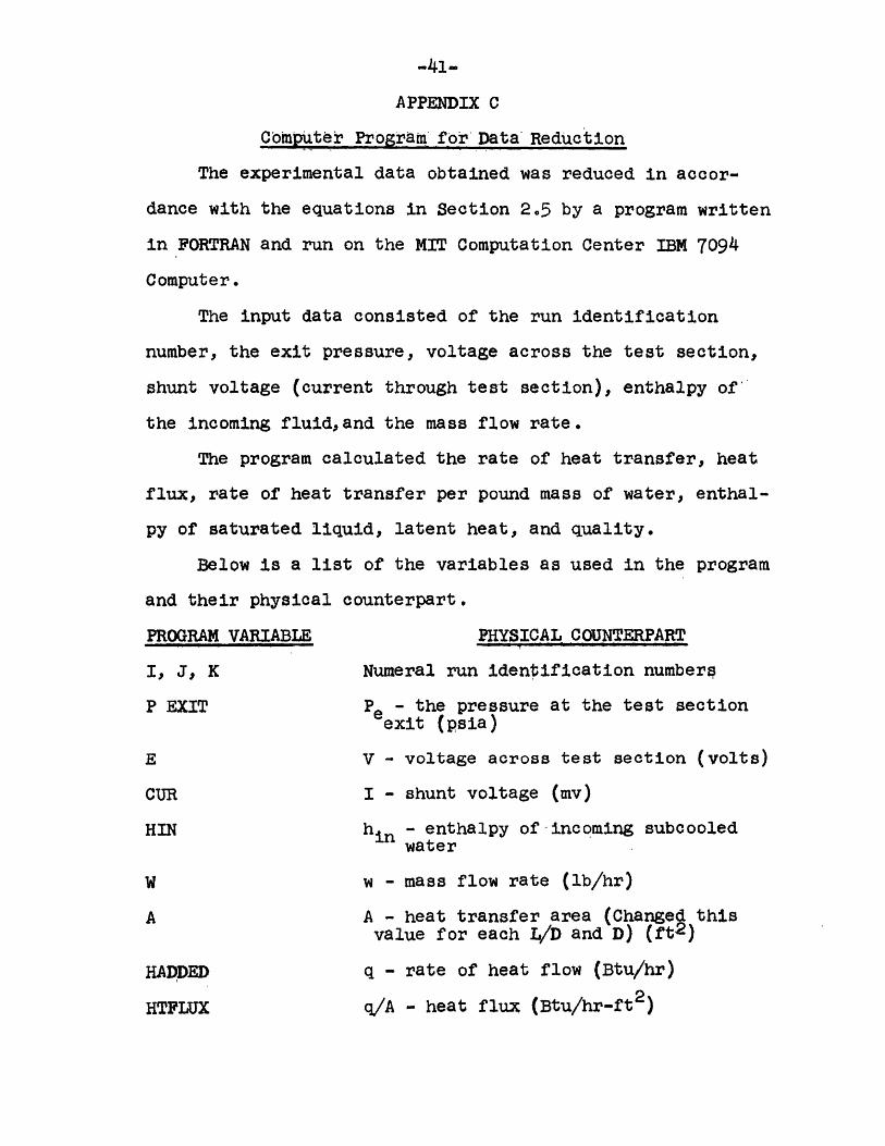
APPENDIX C

Computer Pr ogra: f or' Data Reduction

The experimental data obtained was reduced in accor-

dance with the equations in Section 2.5 by a program written

in FORTRAN and run on the MIT Computation Center IBM 7094

Computer.

The input data consisted of the run identification

number, the exit pressure, voltage across the test section,

shunt voltage (current through test section), enthalpy of'

the incoming fluid,and the mass flow rate.

The program calculated the rate of heat transfer, heat

flux, rate of heat transfer per pound mass of water, enthal-

py of saturated liquid, latent heat, and quality.

Below is a list of the variables as used in the program

and their physical counterpart,

PROGRAM VARIABLE PHYSICAL COUNTERPART

I, J, K Numeral run identification numbers

P EXIT P - the pressure at the test section

E

CUR

HIN

WA

HADDED

HTFLUX

1r0exit (psia)

V - voltage across test section (volts)

I - shunt voltage (mv)

hin - enthalpy of-incoming subcooledwater

w - mass flow rate (lb/hr)

A - heat transfer area (Changed thisvalue for each L/D and D) (ft2)

q - rate of heat flow (Btu/hr)

q/A - heat flux (Btu/hr-ft2)

-42-

BTULBM q/w - rate of heat flow per lbm ofwater (Btu/hr-lbm)

ENFPX hfe - enthalpy of saturated liquid atexit (Btu/lbm)

ENFGPX hfge - latent heat at exit (Btu/lbm)

X x - quality

The enthalpy of saturated liquid (hf) as a function

of pressure was obtained by Todreas(25) by a power series

fit of the Keenan and Keyes' values. For P ( 200 psia

9hf(P) = Z a P

i=o

where

a = 1.1222734(102) a = 2.1239014(l0~)

a I = 6.3204790(100) a6 = -1.0067598(l0~9)

a2 = -l.4742752(lC1~) ay 7 2,9480958(lo-12

a3 = 2.5403593(10'3) a 8 = -48430355(10-15)

a4 = -2.8788220(10-5) a9 = 3.4075972(lo-8

The latent heat (hfg) was obtained by fitting the

Keenan and Keyes' values on a power series, For P (400 psia,

9hfg(P) = aP

i=o

a= 9.9704457(102) a5 = -1.2499843(l09)

a = -2.1762821(100) a6 = l,9322768(l-12)

a2 1.9558791(102) a = -18023251(10-15)

a 3 = -1.2610018(l0~) a. = 9,2680092(10-19)

a4 = 5.0308804(l0~7) a9 = -2,048643(10-22)

The values of the heat transfer area for the differ-

ent tubes are:

-43-

TUBE A (ft2)

0.242 in. i.d. L/D = 30 0.038274

0.242 60 0.076548

0.242 90 0.114822

0.094 60 0.0154

The output data consisted of all the input variables

and the computed quantities.

The program used for the L/D = 60, D = 0.094-in. test

tube computation follows.

COMPUTATION PIOGRAM

1 READ 2, 1, J, K, PEXIT, E, CUR, HIN, WA = .0154HADDED = 205.36 * E * CURHTFLUX = HADDED / ABTUIBM = HADDED / WP =PEXIT

5 ENFPX = .1222734E2 + 6.3204790*P - 1.4742 52E-l*(P**2)1 +2.5403593E-3 *(P**3) -2.8788220E-5* P**4 +2.12390l4E-7*(P**5)2 -1.0067598E-"9*(P**6) .+2.9480958E-12* P**73 -4.8430355E-15*(P**8) +3.4075972E-l8* (P**9)

6 ENFGPX=L9,9704457E2 -2.1762821*P +1.955879lE-2*(P**2)1 -1.2610018E-4*(P**3) +5.0308804E-7*(P**4) -1.2499843E-9*(P**5)2 +1.9322768E-12*( P**6) .8023251E-15*(P**7)3 +9.2680092E-19*(P**8) -2.0148643E-22*( P**9)

X - (HIN + BTULBM - ENFPX)/ENPGPXPRINT 3, I, J, K, PEXIT, E,

1 CUR, HIN, W, HADDED, HTFLUX, BTULBM, X, ENFPX, ENFGPXGO TO 1

2 FORMAT (315,5E10.2)3 FORMAT (7HORUN NOI3, lH-, 13, 1H-,13,5X,1 6HPEXIT=E15.6,5X,2HE=E15.6,5x,4HCUR=E15.6/5x,2 4HHIN=El5.6,5xHW=E15.6,5X,73 HHADDED=E15.6/5X,7HHTFLUX=E15.6,5X,4 7HBTULBM=E15. 6,5X, 2HX=E15.6/5X5 6HENFPx=E15.6, 5X,7HENFGPX=E15.6)END

-44-

APPENDIX D

Incipient Boiling' Analysis

The effects of velocity, temperatureand pressure on

the incipient boiling heat flux, (g/A)i, can be examined by

means of the correlations given in Ref. 22. This correla-

tion for water is:2.30

(q/A), = 15.60 P 156 (TT)P0234 (DI)

For a uniformly heated tube the heat flux can be calculated

from:

(q/A) = h(Tw-Tb) = h (Tw-Ts) + (Ts-Tb) (D2)

The saturation temperature is known from the exit pressure.

The bulk temperature is found by the First Law:

q = c p(Tout-Tin)w (D3)

which leads to:

out w in b(D4)

Since the probe is at the exit, only the conditions at the

exit are of interest and therefore Tb = Tout. The heat

transfer coefficient, h, is found using McAdams' correla-

tion:(2 6 )

(h) = 0.023 (GD) .8( 2.4 (D5)

where the properties are evaluated at the bulk fluid tempera-

ture. For the actual numerical analysis, the values of these

properties came from ElWakil.(27) By assuming a value of

-45-

(q/A), Tb and hence h can be calculated. Then using (D2),

(T -Ts) is found. The values of (q/A) and (T -T ), for

various, G, T , and Pe can then be found and plotted.

Equation (Dl) for the various pressures is then superimposed

on these plots. The intersections of the (q/A) vs. (T -.T5 )

curve and the (q/A) curve is the point at which incipient

boiling is predicted.

This analysis was carried out for the conditions that

were presented in Figs . 28 through 31, i.e.

G x 10- 6 Ti Pelbm/hr-ft2 0F (psia)

a) 0.4 100, 150, 200 30

b) 0.4 100, 200 100

c) 2.0 100, 150, 200 30

d) 2.0 100, 200 100

In Fig. 32a is a representative plot for the conditions in

(c). To visually relate the predicted (q/A), to (x), opera-

ting lines obtained from the formula:

q/w + hi -.hfX = .h fg I(6)hfg

are plotted on coordinates of (q/A) vs x. The (q/A)1 found

from the analysis are plotted on these operating lines and are

connected by a smooth line . This line then is the locus of

predicted (q/A)i for various inlet temperatures. This plot

for conditions (c) above is presented in Fig. 32b. Examin-

ing Fig. 32b it is seen that incipient boiling occurs at

greater subcoolings for lower Ti. From the analysis of

-46-

conditions a, b, dit was also found that incipient boiling

occurs at greater subcooling for larger pressures and, keeping,

P and T constant, at higher G..

0i 0 LLWATER-

........ WESTCO PUMP

ACCUMULATOR

- --------------------------- +DRAIN

FIG. 1 SCHEMATIC LAYOUT OF TEST FACILITY

-48-

BRASS EXITPOWER CONNI

BRASS BUSHINGPOWER CONNECTION

S.S. TESTTUBE

I?

.ET PRESSURETAP

RESISTANCE PROBE AND TEST SECTION

EXITPRESSURE

TAP

POWER CONNECTION

BURNOUT TEST SECTION

TEST SECTION EXITWITH SIGHT SECTION

FIG. 2 DETAILED VIEW OF TEST SECTIONS

PLASTICCLAMP

GROUND

VB

SCOPERv R i = IM.l VI

|| RWL --Nv\r- FLOW

TEST SECTIONFIG. 3a PROBE CIRCUIT DIAGRAM

10 lO 10

Ru-. A

CHARACTERISTICS OF PROBE CIRCUIT

PROBE

FIG. 3b

-50-

3.0

0r-i

0

0 sec 0 .0 4

PHOTO I

P-30, G=0.8x1o6 , T =200, x=-0. 67%

BUBBLY

PHOTO III

Pv3O, G=0.4x1o 6, Ti=150, x=-.201%

SLUG

PHOTO II

P,30, G=2.0x106, T =200, x=-2.81%

BTS TRANSITION

PHOTO IV

P~30, G-2.OxO 6, T =1oo, x=-1.43%

SLUG

FIG. 4 coMPARISON OF PROBE AND SIGHT-SE

(BUBBLY, BUBBLY-TO-SLUG, SLUG)

CTION OBSERVATIONS

-51-

3.0

0

0

O sec 0.04

PHOTO V

P30,, G=2.OxlO , T =100, x=0.25%

FIRST INDICATION OF STA TRANSITION

PHOTO VII

P~-30, G=0.4x106 , T =200, x=10.99%

ANNULAR

PHOTO VI

P'v30, G=0.8x1 00, T.=100, x=2. 42%

STA TRANSITION

PHOTO VIII

P~30, G=1.2x10 6, T =100, x=7.7%

ANNULAR

FIG. 5 COMPARISON OF PROBE AND SIGHT-SECTION OBSERVATIONS

(SLUG-TO-ANNULAR, ANNULAR)

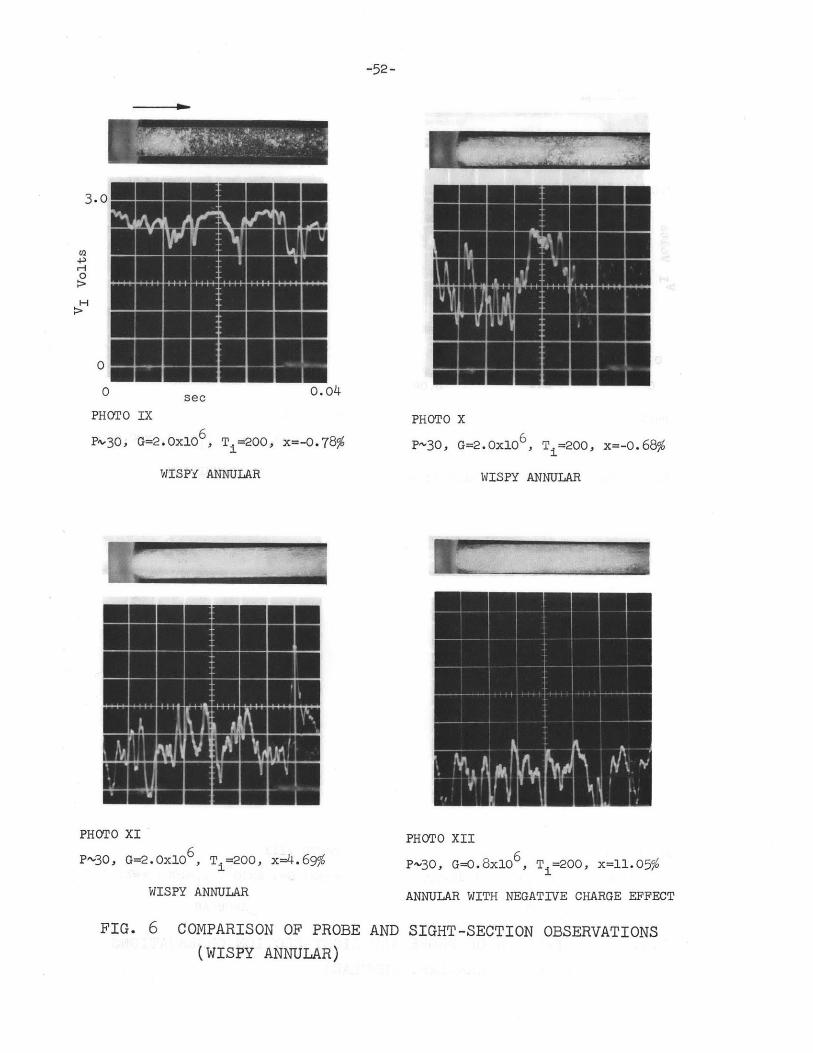
-52-

3.0

-0

0

0 sec o.o4PHOTO IX

PA.30, G=2.Ox1O 6, T =2oo, x=-o.78%

WISPY ANNULAR

PHOTO X

P~30, G=2.0x106, T =200, x=-0.68%

WISPY ANNULAR

PHOTO XI

P~30, G=2.0x106, T =200, x=4.69%

WISPY ANNULAR

PHOTO XII

P"-30, G=<.8x106 , T =200, x=11.05%

ANNULAR WITH NEGATIVE CHARGE EFFECT

FIG. 6 COMPARISON OF PROBE AND SIGHT-SECTION OBSERVATIONS

(WISPY ANNULAR)

7, 774"!

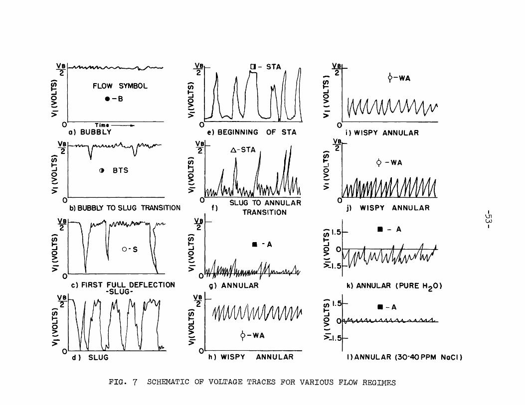
FLOW SYMBOL

O-B

0 Timea) BUBBLY e) BEGINNING OF STA

c-WA

i) WISPY ANNULAR

I BTS

b) BUBBLY TO SLUG TRANSITION

o-S

c) FIRST FULL DEFLECTION-SLUG-

2

f) SLUG TO ANNULARf) TRANSITION

S -A s-j0>-0

I I , 'Ir I ,vovY

g) ANNULARVB~f

p-WA

j) WISPY ANNULAR

U- A

I Al A /I

Kwt/*'QVVk) ANNULAR (PURE H2 0)

IYW/VV'VA-WA

0'h) WISPY ANNULAR

n1.5

00

|~- U - A

4AAA AAAA AAAA .%A -.%,AeAA

I)ANNULAR (30-40PPM NaCI)

OF VOLTAGE TRACES FOR VARIOUS FLOW REGIMES

Vs3

0

Vs2

U)-

0

2

VB

0

0d) SLUG

'

FIG. 7 SCHEMATIC

5.5 II - I I I IPe ~u 30PsiaD = 0.242 in.L = 14.5 in.Ti - 100*FWATER PURITY- 9PPM

e \1< A A

STAA A

. U

AU U

I I I IIIII I I I I-10 -9 -8 -7 -6-5 -4 -3-2 -1 6 7

x - percent

FIG. 8 FLOW REGIME MAP - WATER PURITY = 9PPM NaCl

4.03.0 -

E

.0

0CD

2.42.0

1.6

1.21.0

0.8

0.6-

0.4-

0.3-

0.2

I I I I I

I i I i I II I I I

I I I IIPe ~ 30 PsiaD = 0.242 in.I- 14.5 in.., = 100 * FWATER PURITY

I I I III I I I I

~vO.48Megohm -cm

0

0 0 0

BTS0

I I I I I-10 -9 -8 -7 -6

0

0

S00

I I

ST A A

STA" AU

I I I I I I-5 -4 -3 -2 -1 0 1 2 3 4 5 6 7

x- percent

FIG. 9 FLOW REGIME MAP - WATER PURITY = 0.48 Megohm-cm

5. h)

4.0-

2.4-2.0

No.-

-cI1.2-

E I.0-

0.8

;0.6-CD

0.4

0.3-

0.2-

5.5

1. 6 0 O1I AA 6

- .2- o cm A 0 3

E 1.0-

0.8 o o o0 A . .

0-0.6 -

B BTS S STA A

0.4- o o

0.3-

0.2- o

-10 -9 -8 -7 -6 -5 -4 -3 -2 -1 0 I 2 3 4 5 6 7

x - percent

FIG. 10 FLOW REGIME MAP - WATER PURITY = 2.5 Megohm-cm

4.0-

3.0-

2.4-2.0-

I ~~ I1 II I I I5.5 I I II

Pe"- 30 PsiaD =0.242in.L = 14.5 in.Ti= 150*F

-9 -8 -7 -6 -5 -4 -3 -2 -1 0 I 2 3 4

m U

5 6

x - percent

FLOW REGIME MAP - T. = 150 0 F, LOW PRESSURE

0 0 a aU

0 0 01o U1 U

* * 0 o0 A m= a

e a 0 0 A A a E a

* 0 0 0 0o DA A

B BTS S STA

**e *@0 0 oi A

0 * @ o0 0 i

C~j

0

C

0

1.2

1.0

0.8

0.6

0.4

0.3-

0.2

FIG. 11

I I I I I I I I I II III I I I I

0 00 40 Qu A U E

1.0-E-008- 0 0 e 1 o aA U

40w

00

0.4- ** 00 11 A U "

0.3- -

0.2 0 0 0 a

-10 -9 -8 -7 -6 -5 -4 -3 -2 - 0 I 2 3 4 5 6

x - percent

FIG. 12 FLOW REGIME MAP - T = 200*F, LOW PRESSURE

1.6 -D o 3 ( 00 0 A U -

S1. 2 co 0 0 0 alAA U

E 1.0 - ~~0

w 0.8+ 000"0x 0.6 B BTS S STA A

0.4 0 I A N U m-

0.3-

0.2-

-10 -9 -8 -7 -6 5 -4 -3 -2 -1 0 I 2 3 4 5 6 7

x-percent

FIG. 13 FLOW REGIME MAP - HIGH PRESSURE, T. = 100*O

I I iPe - 100 Psi a

- =0.242in.L: 14.5 in.

- Ti 200*F

I II I i I I I I I

* e

* e 0

* 0

oo0 oil

0 00 0 a A

00 0 A

SCo o o3 3

0 (3 0 0

B BTS S

e 3 00

A A a

SAU

STA

- -

I I I I I I I I-10 -9 -8 -7 -6 -5 -4 -3 -2 -1 0 I 2 3 4 5 6 7

x - percent

FLOW REGIME MAP - HIGH PRESSURE, T. = 200*F

5.5

4.0

2.42.0

1.6 -

1.2

1.0

0.8-

0.6

0-

L.

E

0

CD

a

us

0.4K

0.3-

-

0.2-

FIG. 14

Cm-

-1.6- 0 0 o o

1.2 4 0 0 0 a a n-E 1.0 -

0. * * 9 a0 0 C 1616

0x 0.6

0.4 * * * a 00 0 a * =

0.3-B BTS S STA A

0.2 eo 00 a 0 0 u -

-10 -9 -8 -7 -6 -5 -4 -3 -2 -1 0 I 2 3 4 5 6 7x - percent

FIG. 15 FLOW REGIME MAP - L/D = 30

' 1.2- e0 Co 00 o o 3 a11. .. .s .OE:DO.8 -**o 0o0 0.8 - C 1

B BTS S STA A

0.4- 0 Ro o /- A A U E -

0.3-

0.2- * ,o In *

-10 -9 -8 -7 -6 -5 -4 -3 -2 -1 0 I 2 3 4 5 6 7

x - percent

FIG. 16 FLOW REGIME MAP - L/D = 90

I I I I IPeo~ 100 PsiaD = 0.242 in.L a 21.8 in.

I I I I I I I II

Ti a 1 00*F-0e

0 0 Iii

0 0 o A

0 o i

3TS S

S00

STA

A a U

I I I I I I I I I I | | | |I-10 -9 -8 -7 -6 -5 -4 -3 -2 -1 0 I 2 3 4 5 6

x - percent

FIG. 17 FLOW REGIME MAP - L/D = 90, HIGH PRESSURE

5.5

4.0-

4-to-

E.0

0Ox0

3.0

2.42.0

1.6

1.21.0

0.8

0.6

0.4

0.3-

0.2-

U U * U-

U -~

U-

,

5.5 I I - I I II I IPe"~ 30 PsiaD= 0.09 4 in.L= 5.6 in.Ti 100 F

o 0 A

0 0

00 r

0 0 0 £

)0 0 A6

S Si

o o cs

AsU

0 h

A

0.2--9 -8 -7 -6 -5 -4 -3

I I I-2 -1 0 I 2 3 4 5 6 7

x- percent

FIG. 18 FLOW REGIME MAP - D = 0.094 in., T.

4.0-

3.0K-0

40-

.

E.0

x(D

2.42.0

1.6

1.2

1.0

0.8

0.6

0.4

0.3-

9

A

m

A

-10

= 100*OF

I I I I I

I I

I I I I

I I I I

Pe~. 30 PsiaD = 0.094 in.L 5.60 in.T= 2000F

I I I I

STA

A

I I I I I I I I I I I-10 -9 -8 -7 -6 -5 -4 -3 -2 -1 0 1 2 3 4 5 6 7

x - percent

FIG. 19 FLOW REGIME MAP - D = 0.094 in., Ti = 200*F

5.5

4.0

3.0-

I 11I

WA

N

E.0

0o

x0

2.4

2.0

1.6

1.2

1.0

0.8

0.6~

0.4

0.3-

0.2-

Ua.

A

a

-

C~j4--

E.0

0

x - percent

FIG. 20 FLOW REGIME MAP - VERTICAL UPFLOW

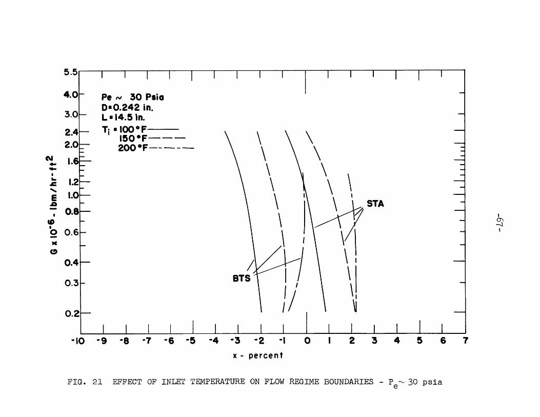
L4i

E

0

sc0

-10 -9 -8 -7 -6 -5 -4 -3 -2 -1 0 1 2 3 4 5 6 7

x - percent

FIG. 21 EFFECT OF INLET TEMPERATURE ON FLOW REGIME BOUNDARIES - P e- 30 psia

5. 1 I I III I IIPe ~ 100 PsiaD :0.242 in.L= 14.5 in.Ti 100 F

BTS

I I II

STA

\

0.2

II II I I I I I I I I_ I --10 -9 -8 -7 -6 -5 -4 -3 -2 -1 0 I 2 3 4 5 6 7

x - percent

OF INLET TEMPERATURE ON FLOW REGIME BOUNDARIES - P 100 psia

4-.

E.0

'o,<

2.42.0

1.21.0

0.8

0.6-

0.4

0.3r-

FIG. 22 EFFECT

4.0 -

3.0 -Ti = 200 *F---

-

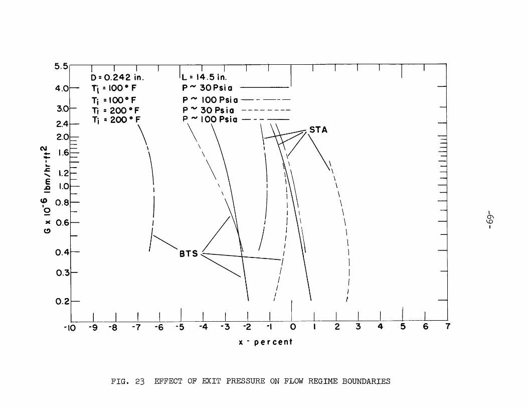
5.5 I I I II I IIID = 0.242 in.T' = 1000 F

=100* F200*F

=200 *I

L=~

4.5 in.r 3u ri a

100 Psia30 Psia100 Psia

STA

4.0-3.0~

P owP-'1P ~

BTS

I I I I I I I I I I I-9 -8 -7 -6 -5 -4 -3 -2 -1 0 I 2 3 4 5 6 7

x - percent

FIG. 23 EFFECT OF EXIT PRESSURE ON FLOW REGIME BOUNDARIES

I"//

CL

4-E

03'

C0

2.42.0

1.6

1.21.0

0.8

0.6

0.4

0.3-

0.2

-10

5.5 I i I I I

5.

III I I

I

4.0-

3.0 -

Pe ~ 30 PsiaD = 0.242 in.L = 14.5 in.Ti= 100 * FWATER PURITY2.5 Megohm-cm----0.48Megohm-cm---9PPM (NoCI)

BTS

10 -9 -8 -7 -6 -5 -4 -3 -2 -I 0 I 2 3 4 5 6 7

x- percent

FIG. 24 EFFECT OF WATER PURITY ON FLOW REGIME BOUNDARIES

2.42.0

1.6

1.2

1.0

0.8

.-

E

0.o

0>

lv-.

I

I

I

I

0.6-

0.4-

0.3-

0.2-

5%-

STA

I

E. 1.6-

.0

0.8 \ /STA

o - 'I0 -0.6 --

0.4 ~ BT S ~--j0.3 -

0.2 (-

i i i il! I i-10 -9 -8 -7 -6 -5 -4 -3 -2 - 0 I 2 3 4 5 6 7

x - percent

FIG. 25 EFFECT OF LENGTH ON FLOW REGIME BOUNDARIES

5.5

.6

e 1.2S.0 BT S STAE 1.0 -

0.8-

10 I /'/ -

0.4 -

0.3--

0.2-

-10 -9 -8 -7 -6 -5 -4 -3 -2 -1 0 1 2 3 4 5 6 7

x - percent

FIG. 26 EFFECT OF DIAMETER ON FLOW REGIME BOUNDARIES

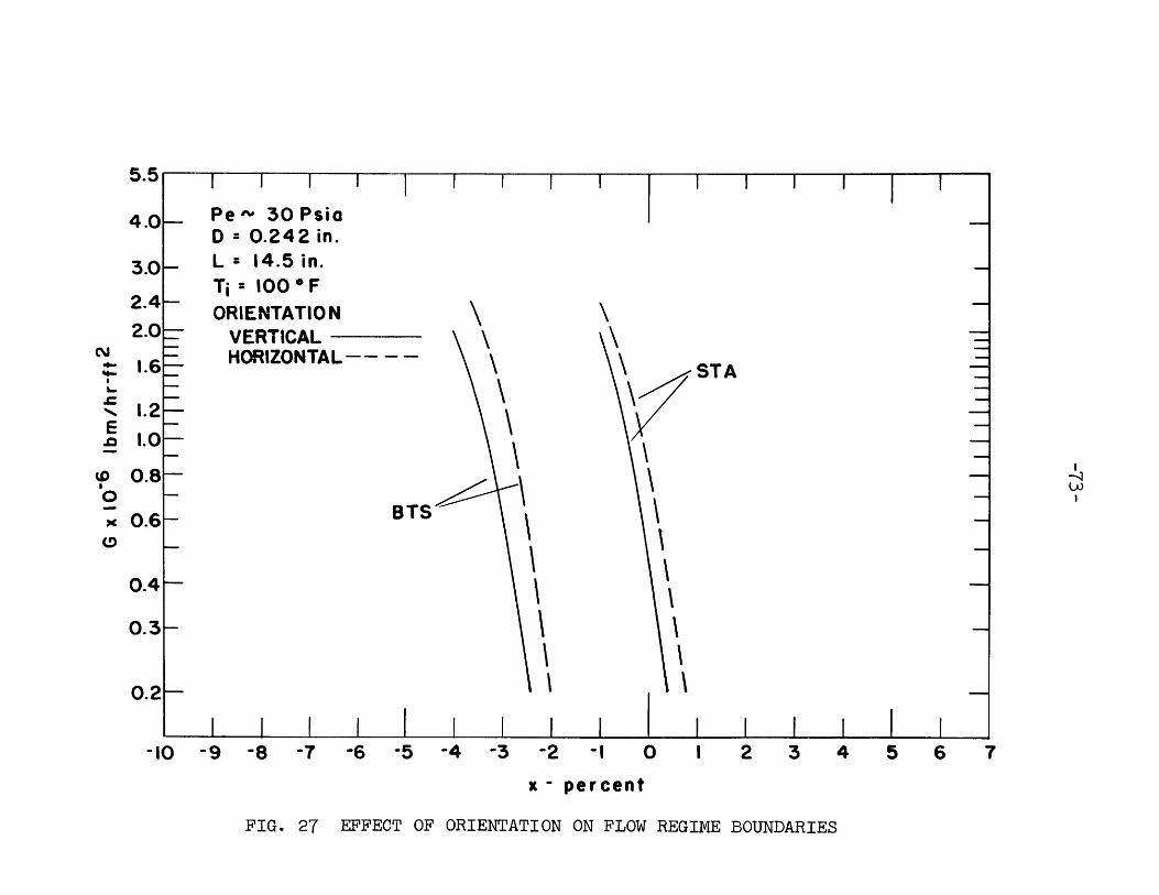
5. I I I I

Pe ~ 30 PsiaD = 0.242 in.

I I I I

4.0-_

3.0 -

-10 -9

STA

L 14.5 in.Ti 100*FORIENTATION

VERTICALHORIZONTAL-- - -

BTS

L I I I I I-8 -7 -6 -5 -4 -3 -2 - 0 I 2 3 4 5 6

x - percent

FIG. 27 EFFECT OF ORIENTATION ON FLOW REGIME BOUNDARIES

.4-4.-

E.0

0

O

2.42.0

1.6

1.21.0

0.8

0.6-

0.4

0.3-

0.2 -

5.5 i I I I I

I i

II

0.31

0.2

0.21

0 ' 1 1 1 1 1

-10 -9 -8 -7 -6 -5 -4 -3 -2 -1 0 1 2 3 4 5 6 7 8

x - percent

FIG. 28 FLOW REGIME MAg ON HEAT FYUX vs. QUALITYG = 0.4 X 10 lbm/hr-f t , LOW PRESSURE

CO-ORDINATES -

(0

0

Cr

I | I I I I I

G = 0.4 x 106 Ibm/hr-ft 2Pe ~ 100 PsiaD= 0.242 in.L= 14.5 in.

I I

Tj=100*F

. Ti= 200OF

I I I I-9 -8 -7

I I I I-6 -5 -4 -3

I I I I I _____

-2 -1 0 1 2 3 4 5 6 7 8

x - percent

FIG. 29 FLOW REGIME MAP ON HEAT FLUX vs. QUALITY CO-ORDINATESG = 0.4 x 1o6 lbm/hr-ft2 , HIGH PRESSURE

I I

0.5--N

10x

4rft'

0.4K-

0. 31-

0.2F-

0.1 -

f

-10I

I I

'

| | I |I

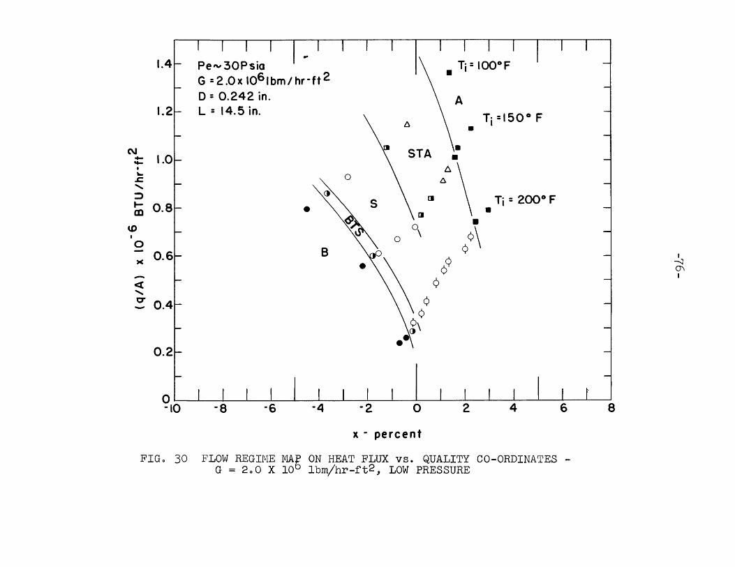
OID

0

4

x - percent

FIG. 30 FLOW REGIME MAG = 2.0 X 10

ON HEAT FLUX vs. QUALITYlbm/hr-ft2 , LOW PRESSURE

CO-ORDINATES -

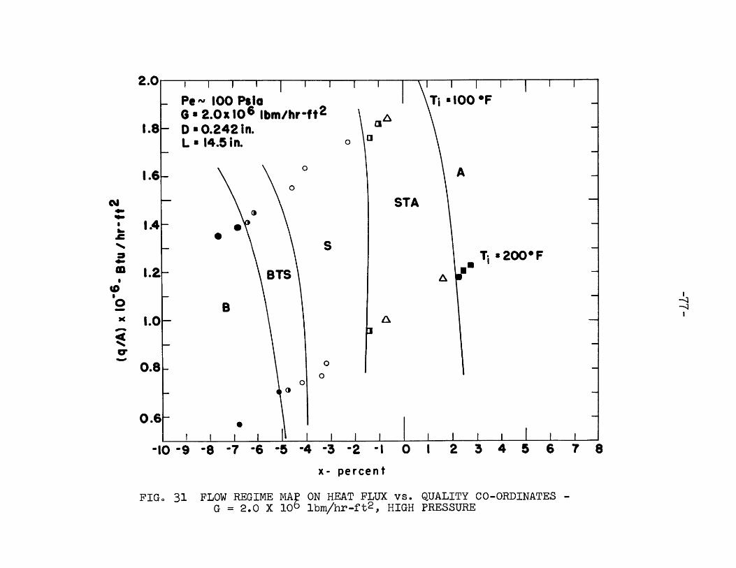
0 4

-10 -9 -8 -7 -6 -5 -4 -3 -2 -1 0 1 2 3 4 5 6

x- percent

FIG. 31 FLOW REGIME MAE ON HEAT FLUX vs. QUALITY CO-ORDINATES -G = 2.0 X 10 lbm/hr-ft2, HIGH PRESSURE

2.4

I .1

1 .

4-

S

cr

ot0

1.2

1.0

0.8

0.61

7 8

-78-

N ~ L =14.5 i n.

S4- Tj 100* F

o -- Ti 150 * F-

0-2-

x

Tj=z2OO *F0 PREDICTED INCIPIENT

BOILING POINTS

I 2 4 6 8 10 20 40 60 80 100(Tw Tsat ) *F

FIG. 32a INCIPIENT BOILING CALCULATIONS

1. 51 1 2G= 2.0x106 Ibm/hr-ft2

N Pe = 30 Psia Ti=100*FI.- D =0.242 in.L 1.0- L = 14.5 in.

LOCUS OF PREDICTED Ti=150*FC o INCIPIENT BOILING

o 0.5_ POINTS

0.4 Ti=2O*F-0.3-o

Z0.2-Cr0.1-

0 -

-14 -12 -10 -8 -6 -4 -2 0

x - percent

FIG. 32b SAMPLE OPERATING LINES SHOWING LOCUS OF INCIPIENT BOILING POINTS

D = 0.094 in.

L = 4.7 in.

G = 0.5 x10 6 Ibm /hr-ft 2

psia

Data of Lopina

-10

(10).00e

-0 B-000

Tj 12 0,, - -, 10.,

|60200

ANNULAR.0, ., 0.

10 20 30 40 50x - percent

AND FLOW PATTERNS FOR TYPICAL CRITICAL HEAT FLUX DATA

2.5

2.04-

co

(0

0O

1.5

1.0

A

0. 5 -

01-3 0 -20 60 70

Pe c-e5 0

FIG. 33 OPERATING LINES

-80-

BIBLIOGRAPHY

1. Gouse, S.W. Jr., "An Introduction to Two-Phase Gas Liq-uid Flow" MIT Engineering Projects Laboratory Report8734-3, June, 1964.

2. Baker, Ovid, "Simultaneous Flow of Oil and Gas," Oiland Gas Jour., Vol. 53, 1954, pp. 185-195.

3. Martinelli, R.C., and D.B. Nelson, "Prediction ofPressure Drop During Forced-Circulation Boiling ofWater", Trans. ASME, Vol. 70, 1948, pp. 695-702.

4. Lavin, J.G., and E.H. Young, "Heat Transfer to Evapora-ting Refrigerants in Two-Phase Flow", AICHE reprint ofpaper presented at the Symp. on Two-Phase Flow and HeatTransfer, Memphis, Tenn., Feb. 2-5, 1964.

5. Griffith, P., "Two-Phase Flow-Regime Detection", ASMEPaper No. 64-WA/HT-43.

6. Hsu, Y.Y., and R.W. Graham, "A Visual Study of Two-Phase Flow in a Vertical Tube with Heat Addition", NASATN D-1564, January, 1963.

7. Suo, M., A.E. Bergles, E.F. Boyle, L. Clawson and P.Goldberg, "Investigation of Boiling Flow Regimes andCritical Heat Flux" Dynatech Corporation Report,NYO-3304-3, March 1, 1965.

8. Bergles, A.E., and M. Suo, "Investigation of BoilingWater Flow Regimes at High Pressures", Dynatech Corpor-ation Report, NYO-3304-8, 1966.

9. BennettA.W., G.F. Hewitt, J.G. Collier, R.K.F. Keeys,P.M.C. Lacey, "Flow Visualization Study of Boiling atHigh Pressure", AERE-R4874, 1965.

10. Lopina, R.F., "Two-Phase Critical Heat Flux to LowPressure Water Flowing in Small Diameter Tubes", SMThesis, Dept. ofMech.Eng., MIT, June, 1965.

11. Vohr, J.H., "Flow Patterns of Two-Phase Flow - A Surveyof Literature", TID 11514, AEC, December, 1960.

12. Kepple, R.R., and T.V. Tung, "Two Phase (Gas-Liquid)System Heat Transfer and Hydraulics (An AnnotatedBibliography)", ANL-6734, July, 1963.

13. Solomon, J.V., "Construction of a Two-Phase Flow RegimeTransition Detector", SM Thesis, Dept. of Mech. Eng.,MIT, June, 1962.

14. Nassos, G.P., "Development of an Electrical ResistivityProbe for Void Fraction Measurements in Air Water Flow ,

ANL-6738, June, 1963.

15. Haberstroh, R.D., and P. Griffith, "The Transition fromthe Annular to the Slug Flow Regime in Two-Phase Flow",MIT Engineering Projects Laboriatory Report 5003-28,July, 1964.

16. Griffith, P., "The Slug-Annular Flow Regime at ElevatedPressure", ANL-6796, November, 1963.

17. Bergles, A.E., and W.M. Rohsenow, "Forced ConvectionSurface Boiling Heat Transfer and -Burnout in Tubes ofSmall Diameter", MIT Engineering Projects Laboratory-Report 8767-21, May, 1962.

18. Keily, D.P., Meteorology Dept., MIT, Personal Communi-cation, August 12, 1965.

19. Vonnegut, B., A. Doyle, and D. Moffet, "Behavior ofEvaporating Electrically Charged Droplets", Jour. ofColloid Science, Vol. 19, 1964, p. 136.

20. Suo, M., Mechanical Engineering Department, MIT,Personal Communication, May, 1965. Professor Suo'scalculations were based on Glasstone's, "PhysicalChemistry".

21. Radoveich, N.A., and R. Moissis, "The Transition FromTwo-Phase Bubble Flow to Slug Flow", MIT EngineeringProject Laboratory Report 7-7673-22, June, 1962.

22. Bergles, A.E., and W.M. Rohsenow, "The Determinationof Forced-Convection Surface Boiling Heat Transfer",Trans. ASME, Jour. of Heat Transfer, Vol. 86, 1964,pp. 365-372.

23. Bowring, R.W., "Physical Model, Based on Bubble De-tachment, and Calculation of Steam Voidage in the Sub-cooled Region of a Heated Channel", Report -HPR 10, OECDHalden Reactor Project, December, 1962.

24. Hewitt, G.F., H.A. Hearsey, P.M.C. Lacey, and D.J.Pulling, "Burnout and Film Flow in the Evaporation ofWater in Tubes", AERE-R 4864, March, 1965.

25. Todreas, N.E., and W.M. Rohsenow, "The Effect of Non-Uniform Axial Heat Flux Distribution", MIT EngineeringProjects Laboratory Report No. 9843-37, September, 1965.

26. Rohsenow, W.M., and H. Choi, Heat, Mass, and MomentumTransfer, Prentice-Hall, 1963.

27. ElWakil, M.M., Nuclear Power Engineering, McGraw-Hill,1962.