A STUDY IN GPS-DENIED NAVIGATION USING SYNTHETIC APERTURE RADAR

by

Colton P. Lindstrom

A thesis submitted in partial fulfillmentof the requirements for the degree

of

MASTER OF SCIENCE

in

Electrical Engineering

Approved:

Randall S. Christensen, Ph.D. Jacob H. Gunther, Ph.D.Major Professor Committee Member

Charles M. Swenson, Ph.D. D. Richard Cutler, Ph.D.Committee Member Interim Vice Provost for Graduate Studies

UTAH STATE UNIVERSITYLogan, Utah

2020

ii

Copyright © Colton P. Lindstrom 2020

All Rights Reserved

iii

ABSTRACT

A Study in GPS-Denied Navigation Using Synthetic Aperture Radar

by

Colton P. Lindstrom, Master of Science

Utah State University, 2020

Major Professor: Randall S. Christensen, Ph.D.Department: Electrical and Computer Engineering

GPS denied navigation solves the problem of precisely navigating a vehicle in the

absence of a Global Navigation Satellite System such as GPS. Several methods of navigation

without GPS have been proposed and studied. The research presented in this thesis furthers

the work done in this field by investigating how synthetic aperture radar (SAR) could be

used in a GPS denied navigation scenario.

A compilation of three academic papers is presented. Each paper explores an individual

aspect of the proposed problem, and the results from each are reported. The results support

the use of SAR in GPS denied navigation settings. Derivations, background theory, and

validation methods are provided throughout this document.

The major contributions from this research are threefold. First, a system in imple-

mented that synthesizes pseudo range and range rate measurements within an Inertial Nav-

igation System (INS) architecture employing an extended Kalman filter (EKF). The system

is tested in a GPS denied navigation setting to test the feasibility of using radar telemetry

for navigation. Results suggest that navigation using radar telemetry in A GPS denied

setting is feasible and results in converging and bounded navigation estimation errors.

Second, the relationship between navigation errors and SAR imaging errors is explored.

Images are formed using the back-projection algorithm. This investigation is motivated by

iv

the potential of inferring navigation errors from blurs and shifts within an improperly formed

SAR image. Analytical expressions are derived and verified using both real and simulated

navigation and radar data.

Third, a full flight and radar system is developed which investigates navigation from

fully formed SAR images using the range-Doppler algorithm. The system is tested using

both simulated and real flight and radar data. For both types of data, results show a system

that accurately navigates in the absence of GPS with bounded and converging navigation

estimation errors. Results for the case of simulated data are validated via Monte Carlo

analysis.

(181 pages)

v

PUBLIC ABSTRACT

A Study in GPS-Denied Navigation Using Synthetic Aperture Radar

Colton P. Lindstrom

In modern navigation systems, GPS is vital to accurately piloting a vehicle. This is

especially true in autonomous vehicles, such as UAVs, which have no pilot. Unfortunately,

GPS signals can be easily jammed or spoofed. For example, canyons and urban cities create

an environment where the sky is obstructed and make GPS signals unreliable. Additionally,

hostile individuals can transmit personal signals intended to block or spoof GPS signals. In

these situations, it is important to find a means of navigation that doesn’t rely on GPS.

Navigating without GPS means that other types of sensors or instruments must be

used to replace the information lost from GPS. Some examples of additional sensors include

cameras, altimeters, magnetometers, and radar. The work presented in this thesis shows

how radar can be used to navigate without GPS. Specifically, synthetic aperture radar

(SAR) is used, which is a method of processing radar data to form images of a landscape

similar to images captured using a camera.

SAR presents its own unique set of benefits and challenges. One major benefit of SAR

is that it can produce images of an area even at night or through cloud cover. Additionally,

SAR can image a wide swath of land at an angle that would be difficult for a camera

to achieve. However, SAR is more computationally complex than other imaging sensors.

Image quality is also highly dependent on the quality of navigation information available.

In general, SAR requires that good navigation data be had in order to form SAR

images. The research here explores the reverse problem where SAR images are formed

without good navigation data and then good navigation data is inferred from the images.

This thesis performs feasibility studies and real data implementations that show how

SAR can be used in navigation without the presence of GPS. Derivations and background

vi

materials are provided. Validation methods and additional discussions are provided on the

results of each portion of research.

vii

ACKNOWLEDGMENTS

I want to express my thanks to my major professor, Dr. Randall Christensen, and to

my committee, Dr. Jacob Gunther and Dr. Charles Swenson. A huge thanks goes to my

wife for her patience and support. A thanks also goes to Sandia National Laboratories, who

funded a large portion of this research. I also thank the Space Dynamics Laboratory for

providing flight and radar test data for this research.

Colton P. Lindstrom

viii

CONTENTS

Page

ABSTRACT . . . . . . . . . . . . . . . . . . . . . . . . . . . . . . . . . . . . . . . . . . . . . . . . . . . . . . iii

PUBLIC ABSTRACT . . . . . . . . . . . . . . . . . . . . . . . . . . . . . . . . . . . . . . . . . . . . . . . v

ACKNOWLEDGMENTS . . . . . . . . . . . . . . . . . . . . . . . . . . . . . . . . . . . . . . . . . . . . vii

LIST OF TABLES . . . . . . . . . . . . . . . . . . . . . . . . . . . . . . . . . . . . . . . . . . . . . . . . . xi

LIST OF FIGURES . . . . . . . . . . . . . . . . . . . . . . . . . . . . . . . . . . . . . . . . . . . . . . . . xii

ACRONYMS . . . . . . . . . . . . . . . . . . . . . . . . . . . . . . . . . . . . . . . . . . . . . . . . . . . . .xviii

1 INTRODUCTION . . . . . . . . . . . . . . . . . . . . . . . . . . . . . . . . . . . . . . . . . . . . . . . 1

2 BACKGROUND . . . . . . . . . . . . . . . . . . . . . . . . . . . . . . . . . . . . . . . . . . . . . . . . 52.1 Inertial Navigation System Structure . . . . . . . . . . . . . . . . . . . . . . 52.2 Synthetic Aperture Radar Processing . . . . . . . . . . . . . . . . . . . . . . 7

3 AN INVESTIGATION OF GPS-DENIED NAVIGATION USING AIRBORNE RADARTELEMETRY . . . . . . . . . . . . . . . . . . . . . . . . . . . . . . . . . . . . . . . . . . . . . . . . . . . . 11

3.1 Introduction . . . . . . . . . . . . . . . . . . . . . . . . . . . . . . . . . . . . 113.2 Literature Review . . . . . . . . . . . . . . . . . . . . . . . . . . . . . . . . 123.3 Method . . . . . . . . . . . . . . . . . . . . . . . . . . . . . . . . . . . . . . 133.4 State and Model Definitions . . . . . . . . . . . . . . . . . . . . . . . . . . . 153.5 Measurement Model . . . . . . . . . . . . . . . . . . . . . . . . . . . . . . . 193.6 Covariance Propagation . . . . . . . . . . . . . . . . . . . . . . . . . . . . . 213.7 Kalman Update . . . . . . . . . . . . . . . . . . . . . . . . . . . . . . . . . . 213.8 Filter Validation . . . . . . . . . . . . . . . . . . . . . . . . . . . . . . . . . 223.9 Results . . . . . . . . . . . . . . . . . . . . . . . . . . . . . . . . . . . . . . . 27

3.9.1 Sensitivity to IMU Grade . . . . . . . . . . . . . . . . . . . . . . . . 273.9.2 Sensitivity to SAR Measurement Noise . . . . . . . . . . . . . . . . . 283.9.3 Sensitivity to Platform/Target Geometry . . . . . . . . . . . . . . . 29

3.10 Conclusion . . . . . . . . . . . . . . . . . . . . . . . . . . . . . . . . . . . . 303.11 Acknowledgments . . . . . . . . . . . . . . . . . . . . . . . . . . . . . . . . . 30

4 SENSITIVITY OF BPA SAR IMAGE FORMATION TO INITIAL POSITION,VELOCITY, AND ATTITUDE NAVIGATION ERRORS . . . . . . . . . . . . . . . . . . . . . 34

4.1 Introduction . . . . . . . . . . . . . . . . . . . . . . . . . . . . . . . . . . . . 344.1.1 Motivation . . . . . . . . . . . . . . . . . . . . . . . . . . . . . . . . 354.1.2 Literature Review . . . . . . . . . . . . . . . . . . . . . . . . . . . . 354.1.3 Contributions . . . . . . . . . . . . . . . . . . . . . . . . . . . . . . . 36

4.2 Background . . . . . . . . . . . . . . . . . . . . . . . . . . . . . . . . . . . . 36

ix

4.2.1 Inertial Navigation . . . . . . . . . . . . . . . . . . . . . . . . . . . . 374.2.2 Back-Projection Algorithm . . . . . . . . . . . . . . . . . . . . . . . 41

4.3 Analysis . . . . . . . . . . . . . . . . . . . . . . . . . . . . . . . . . . . . . . 434.3.1 Position Errors . . . . . . . . . . . . . . . . . . . . . . . . . . . . . . 444.3.2 Velocity Errors . . . . . . . . . . . . . . . . . . . . . . . . . . . . . . 454.3.3 Attitude Errors . . . . . . . . . . . . . . . . . . . . . . . . . . . . . . 49

4.4 Simulated Data . . . . . . . . . . . . . . . . . . . . . . . . . . . . . . . . . . 514.5 Real Data . . . . . . . . . . . . . . . . . . . . . . . . . . . . . . . . . . . . . 534.6 Conclusion . . . . . . . . . . . . . . . . . . . . . . . . . . . . . . . . . . . . 54

5 GPS-DENIED NAVIGATION USING SYNTHETIC APERTURE RADAR ANDKNOWN TARGET LOCATIONS . . . . . . . . . . . . . . . . . . . . . . . . . . . . . . . . . . . . . . 61

5.1 Introduction . . . . . . . . . . . . . . . . . . . . . . . . . . . . . . . . . . . . 615.1.1 Literature Review . . . . . . . . . . . . . . . . . . . . . . . . . . . . 62

5.2 Background . . . . . . . . . . . . . . . . . . . . . . . . . . . . . . . . . . . . 675.3 Navigation System and Monte Carlo Framework Development . . . . . . . . 71

5.3.1 Truth and Navigation Models . . . . . . . . . . . . . . . . . . . . . . 725.3.2 Linear Error Model . . . . . . . . . . . . . . . . . . . . . . . . . . . . 745.3.3 Measurement Model . . . . . . . . . . . . . . . . . . . . . . . . . . . 765.3.4 Covariance Propagation . . . . . . . . . . . . . . . . . . . . . . . . . 79

5.4 Results . . . . . . . . . . . . . . . . . . . . . . . . . . . . . . . . . . . . . . . 815.4.1 Simulated Data . . . . . . . . . . . . . . . . . . . . . . . . . . . . . . 815.4.2 Real Data . . . . . . . . . . . . . . . . . . . . . . . . . . . . . . . . . 83

5.5 Conclusion . . . . . . . . . . . . . . . . . . . . . . . . . . . . . . . . . . . . 935.5.1 Future Work . . . . . . . . . . . . . . . . . . . . . . . . . . . . . . . 93

5.6 Appendix . . . . . . . . . . . . . . . . . . . . . . . . . . . . . . . . . . . . . 955.6.1 Autofocus . . . . . . . . . . . . . . . . . . . . . . . . . . . . . . . . . 95

6 CONCLUSION . . . . . . . . . . . . . . . . . . . . . . . . . . . . . . . . . . . . . . . . . . . . . . . . . 98

REFERENCES . . . . . . . . . . . . . . . . . . . . . . . . . . . . . . . . . . . . . . . . . . . . . . . . . . . 100

APPENDICES . . . . . . . . . . . . . . . . . . . . . . . . . . . . . . . . . . . . . . . . . . . . . . . . . . . . 105A Kalman Filter Verification and Debugging Process . . . . . . . . . . . . . . 106

A.1 State Vector Mappings and Validation . . . . . . . . . . . . . . . . . 106A.2 Truth and Navigation State Propagation and Validation . . . . . . . 109A.3 Error State Propagation and Validation . . . . . . . . . . . . . . . . 110A.4 Linear Measurement Validation . . . . . . . . . . . . . . . . . . . . . 114A.5 Covariance Propagation Validation . . . . . . . . . . . . . . . . . . . 116A.6 Kalman Update Validation . . . . . . . . . . . . . . . . . . . . . . . 125

B EKF Related Derivations . . . . . . . . . . . . . . . . . . . . . . . . . . . . . 134B.1 Linearization of Velocity State . . . . . . . . . . . . . . . . . . . . . 134B.2 Linearization of Attitude State . . . . . . . . . . . . . . . . . . . . . 135B.3 Linearization of Measurement Model . . . . . . . . . . . . . . . . . . 137

C Pulse Compression Derivation . . . . . . . . . . . . . . . . . . . . . . . . . . 141D Autofocus . . . . . . . . . . . . . . . . . . . . . . . . . . . . . . . . . . . . . 146

D.1 Range and Range Rate Measurements . . . . . . . . . . . . . . . . . 146

x

D.2 Autofocus . . . . . . . . . . . . . . . . . . . . . . . . . . . . . . . . . 149E Spatial Variance and Ambiguities . . . . . . . . . . . . . . . . . . . . . . . . 158F Copyright Information . . . . . . . . . . . . . . . . . . . . . . . . . . . . . . 162

F.1 Published Works . . . . . . . . . . . . . . . . . . . . . . . . . . . . . 162F.2 Works Submitted for Publication . . . . . . . . . . . . . . . . . . . . 162

xi

LIST OF TABLES

Table Page

3.1 Noise standard deviations used for SAR and altimeter measurement noises. 27

3.2 Different IMU grades used in investigation expressed as 3σ values. . . . . . 28

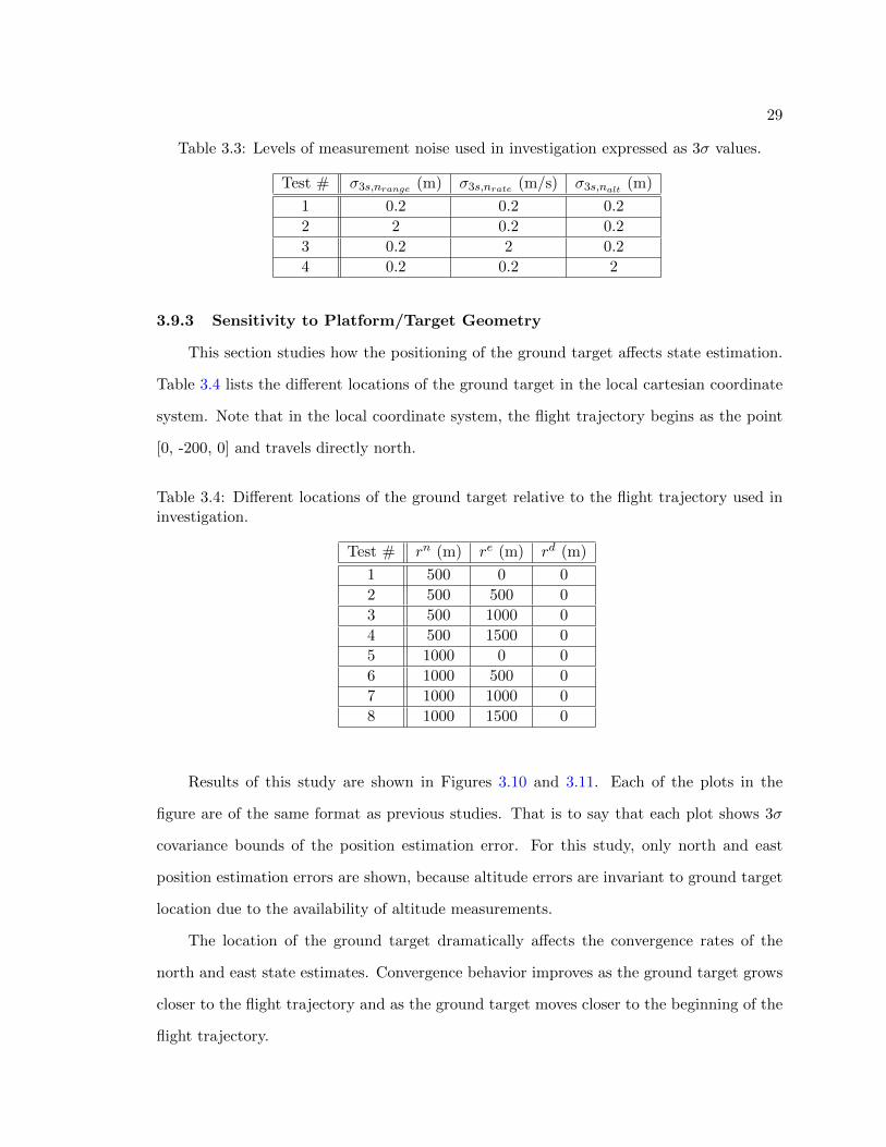
3.3 Levels of measurement noise used in investigation expressed as 3σ values. . 29

3.4 Different locations of the ground target relative to the flight trajectory usedin investigation. . . . . . . . . . . . . . . . . . . . . . . . . . . . . . . . . . . 29

5.1 Summary of radar parameters used in simulation. . . . . . . . . . . . . . . . 82

5.2 Summary of navigation parameters used in simulation. . . . . . . . . . . . . 82

5.3 Summary of radar parameters from the FlexSAR system. . . . . . . . . . . 88

5.4 Summary of navigation parameters from the FlexSAR system. . . . . . . . 88

A.1 Defining truth and error state. . . . . . . . . . . . . . . . . . . . . . . . . . 108

A.2 Estimated state. . . . . . . . . . . . . . . . . . . . . . . . . . . . . . . . . . 108

A.3 Difference between defined error with calculated error. . . . . . . . . . . . . 109

A.4 Difference between defined truth and calculated truth. . . . . . . . . . . . . 109

A.5 Validation of F matrix using a comparison of nonlinear and linear error statesat time t. . . . . . . . . . . . . . . . . . . . . . . . . . . . . . . . . . . . . . 115

A.6 Validation of H matrix by calculating the difference between linear and non-linear residual measurements. . . . . . . . . . . . . . . . . . . . . . . . . . . 116

A.7 3σ values selected by the user for this validation step. . . . . . . . . . . . . 117

A.8 3σ noise values used for covariance propagation validation. . . . . . . . . . . 118

A.9 Noise standard deviations used for SAR and altimeter measurement noises. 125

xii

LIST OF FIGURES

Figure Page

1.1 Categorization of radar aided GPS-denied navigation. . . . . . . . . . . . . 2

2.1 Block diagram of the GPS-denied navigation system. . . . . . . . . . . . . . 5

2.2 Block diagram of the extended Kalman filter. . . . . . . . . . . . . . . . . . 7

2.3 Illustration of how radar pulses are transmitted according to a PRF. . . . . 9

2.4 Illustration of the hyperbolic shape of range compressed data where η isazimuth time and t is range time. . . . . . . . . . . . . . . . . . . . . . . . . 10

3.1 Cross-track and elevation estimates are not unique given a slant range totarget. . . . . . . . . . . . . . . . . . . . . . . . . . . . . . . . . . . . . . . . 14

3.2 Geometry of the UAV relative to the ground target. . . . . . . . . . . . . . 15

3.3 Geometry of range, range rate, and altitude measurements. . . . . . . . . . 20

3.4 Residual measurements after implementation of Kalman updates. From topto bottom: Altimeter residual, range residual, range-rate residual. . . . . . 23

3.5 Monte Carlo simulation with filtered covariance bounds. From top to bottom:North position east position, down position. . . . . . . . . . . . . . . . . . . 24

3.6 Monte Carlo simulation with filtered covariance bounds. From top to bottom:North velocity east velocity, down velocity. . . . . . . . . . . . . . . . . . . 25

3.7 Monte Carlo simulation with filtered covariance bounds. From top to bottom:North attitude east attitude, down attitude. . . . . . . . . . . . . . . . . . . 26

3.8 Position estimation errors expressed as covariance bounds to illustrate IMUgrade differences. From top to bottom: North position, east position, downposition. By line type: Dashed line represents consumer grade, solid linerepresents tactical grade, and dot-dash line represents navigation grade. . . 31

3.9 Position estimation errors expressed as covariance bounds to illustrate mea-surement error differences. From top to bottom: North position, east posi-tion, down position. By line type: Dashed line represents increased rangeerror, dot-dash line represents increased range-rate error, dotted line repre-sents increased altitude error, and solid line represents no increased error. . 32

xiii

3.10 Position estimation errors expressed as covariance bounds to illustrate groundtarget placement. From right to left: North position, east position. Linetypes: Dashed line for target at (500, 0, 0), dot-dash line for target at (500,500, 0), solid line for target at (500, 1000, 0), and dotted line for target at(500, 1500, 0). . . . . . . . . . . . . . . . . . . . . . . . . . . . . . . . . . . . 33

3.11 Position estimation errors expressed as covariance bounds to illustrate groundtarget placement. From right to left: North position, east position. Linetypes: Dashed line for target at (1000, 0, 0), dot-dash line for target at(1000, 500, 0), solid line for target at (1000, 1000, 0), and dotted line fortarget at (1000, 1500, 0). . . . . . . . . . . . . . . . . . . . . . . . . . . . . . 33

4.1 Illustration of how cross track position errors affect the various stages of radarprocessing. Left: flight trajectory with error. Center: range compressed datawith error. Right: final image with error. Light colored or dotted illustrationsrepresent expected data given estimation errors. Solid black illustrationsrepresent truth data. . . . . . . . . . . . . . . . . . . . . . . . . . . . . . . . 46

4.2 Illustration of how along track position errors affect the various stages ofradar processing. Left: flight trajectory with error. Center: range com-pressed data with error. Right: final image with error. Light colored ordotted illustrations represent expected data given estimation errors. Solidblack illustrations represent truth data. . . . . . . . . . . . . . . . . . . . . 46

4.3 Illustration of how elevation position errors affect the various stages of radarprocessing. Left: flight trajectory with error. Center: range compresseddata with error. Right: final image with error. Light colored or dottedillustrations represent expected data given estimation errors. Solid blackillustrations represent truth data. . . . . . . . . . . . . . . . . . . . . . . . . 46

4.4 Illustration of how cross track velocity errors affect the various stages of radarprocessing. Left: flight trajectory with error. Center: range compressed datawith error. Right: final image with error. Light colored or dotted illustrationsrepresent expected data given estimation errors. Solid black illustrationsrepresent truth data. . . . . . . . . . . . . . . . . . . . . . . . . . . . . . . . 47

4.5 Illustration of how along track velocity errors affect the various stages of radarprocessing. Left: flight trajectory with error. Center: range compressed datawith error. Right: final image with error. Light colored or dotted illustrationsrepresent expected data given estimation errors. Solid black illustrationsrepresent truth data. . . . . . . . . . . . . . . . . . . . . . . . . . . . . . . . 47

4.6 Illustration of how elevation velocity errors affect the various stages of radarprocessing. Left: flight trajectory with error. Center: range compresseddata with error. Right: final image with error. Light colored or dottedillustrations represent expected data given estimation errors. Solid blackillustrations represent truth data. . . . . . . . . . . . . . . . . . . . . . . . . 47

xiv

4.7 Progression of roll errors through the SAR data. Left: flight trajectory witherror. Center: range compressed data with error. Right: final image witherror. Light colored or dotted illustrations represent expected data givenestimation errors. Solid black illustrations represent truth data. . . . . . . . 48

4.8 Progression of pitch error through the SAR data. Left: flight trajectory witherror. Center: range compressed data with error. Right: final image witherror. Light colored or dotted illustrations represent expected data givenestimation errors. Solid black illustrations represent truth data. . . . . . . . 48

4.9 Reference image for simulated SAR data. . . . . . . . . . . . . . . . . . . . 52

4.10 Reference image for real SAR data. . . . . . . . . . . . . . . . . . . . . . . . 53

4.11 Position errors in simulated data: Top, along track position error (3 m).Middle, cross track position error (3 m). Bottom, elevation position error (3m). Each figure is superimposed with a reference target location, “X”, anda predicted target shift, “O”. . . . . . . . . . . . . . . . . . . . . . . . . . . 55

4.12 Velocity errors in simulated data: Top, along track velocity error (0.1 m/s).Middle, cross track velocity error (0.05 m/s). Bottom, elevation velocity error(0.05 m/s). Each figure is superimposed with a reference target location, “X”,and a predicted target shift, “O”. . . . . . . . . . . . . . . . . . . . . . . . . 56

4.13 Attitude errors in simulated data: Top, roll error (0.001 rad). Middle, pitcherror (0.02 rad). Bottom, yaw error (0.1 rad). Each figure is superimposedwith a reference target location, “X”, and a predicted target shift, “O”. . . 57

4.14 Position errors in real data: Top, along track position error (3 m). Middle,cross track position error (3 m). Bottom, elevation position error (3 m). Eachfigure is superimposed with a reference target location, “X”, and a predictedtarget shift, “O”. . . . . . . . . . . . . . . . . . . . . . . . . . . . . . . . . . 58

4.15 Velocity errors in real data: Top, along track velocity error (1 m/s). Middle,cross track velocity error (0.2 m/s). Bottom, elevation velocity error (0.2m/s). Each figure is superimposed with a reference target location, “X”, anda predicted target shift, “O”. . . . . . . . . . . . . . . . . . . . . . . . . . . 59

4.16 Attitude errors in real data: Top, roll error (0.01 rad). Middle, pitch error(0.5 rad). Bottom, yaw error (0.1 rad). Each figure is superimposed with areference target location, “X”, and a predicted target shift, “O”. . . . . . . 60

5.1 Illustration of how ground targets at various locations (Left) become hyper-bolic curves in the range compressed data (Right). . . . . . . . . . . . . . . 70

5.2 Illustration of the data in the range Doppler domain before (Left) and after(Right) range cell migration correction. . . . . . . . . . . . . . . . . . . . . 70

xv

5.3 Fully formed SAR image after azimuth matched filtering and inverse FFT. . 72

5.4 Illustrates the process of calculating radar measurements. A reference image(distinguished using solid lines) and an image formed using the estimatedflight trajectory (distinguished using dotted lines) are cross correlated witheach other. Offsets in range, ∆R, and cross range, ∆CR, appear in the crosscorrelation as a shift in the main peak. . . . . . . . . . . . . . . . . . . . . . 77

5.5 Measurement residuals for altimeter measurements (Top), range measure-ments (Middle), and cross range measurements (Bottom). Dotted lines sig-nify 3 sigma bounds, and solid lines represent residual measurements. . . . 84

5.6 Estimation errors for north position (Top), east position (Middle), and downposition (Bottom). Dotted lines signify 3 sigma bounds. Individual solidlines represent individual runs of the Monte Carlo simulation. . . . . . . . . 85

5.7 Estimation errors for north velocity (Top), east velocity (Middle), and downvelocity (Bottom). Dotted lines signify 3 sigma bounds. Individual solid linesrepresent individual runs of the Monte Carlo simulation. . . . . . . . . . . . 86

5.8 Estimation errors for north attitude (Top), east attitude (Middle), and downattitude (Bottom). Dotted lines signify 3 sigma bounds. Individual solidlines represent individual runs of the Monte Carlo simulation. . . . . . . . . 87

5.9 Measurement residuals from the real data set for the altimeter measurements(Top), range measurements (Middle), and cross range measurements (Bot-tom). Dotted lines signify 3 sigma bounds, and solid lines represent residualmeasurements. . . . . . . . . . . . . . . . . . . . . . . . . . . . . . . . . . . 89

5.10 Estimation errors from the real data set for north position (Top), east position(Middle), and down position (Bottom). Dotted lines signify 3 sigma bounds.Solid lines represent actual estimation error. . . . . . . . . . . . . . . . . . . 90

5.11 Estimation errors from the real data set for north velocity (Top), east velocity(Middle), and down velocity (Bottom). Dotted lines signify 3 sigma bounds.Solid lines represent actual estimation error. . . . . . . . . . . . . . . . . . . 91

5.12 Estimation errors from the real data set for north attitude (Top), east at-titude (Middle), and down attitude (Bottom). Dotted lines signify 3 sigmabounds. Solid lines represent actual estimation error. . . . . . . . . . . . . . 92

5.13 Comparison of position estimation error bounds while using SAR measure-ments and while omitting SAR measurements. Dotted lines indicate thebounds given omission of SAR measurements. Solid lines indicate the boundsgiven the use of SAR measurements. . . . . . . . . . . . . . . . . . . . . . . 94

xvi

5.14 Comparison of a blurry SAR image before (Top) and after (Bottom) azimuthmisregistration autofocusing. . . . . . . . . . . . . . . . . . . . . . . . . . . 97

A.1 Trajectory of UAV using true measurements from an IMU. . . . . . . . . . 110

A.2 Errors in the position, velocity, and attitude between the truth and navigationmodels. . . . . . . . . . . . . . . . . . . . . . . . . . . . . . . . . . . . . . . 111

A.3 Errors of the bias states, which are all zero with no noise propagation. . . . 112

A.4 Residual errors between the true measurements and estimated measurements. 113

A.5 Hairline plot showing the propagation errors in position. From top to bottom:North position error, east position error, down position error. . . . . . . . . 119

A.6 Hairline plot showing the propagation errors in velocity. From top to bottom:North velocity error, east velocity error, down velocity error. . . . . . . . . 120

A.7 Hairline plot showing the propagation errors in attitude. From top to bottom:North attitude error, east attitude error, down attitude error. . . . . . . . . 121

A.8 Hairline plot showing the propagation errors in accelerometer bias. Fromtop to bottom: X accelerometer bias error, Y accelerometer bias error, Zaccelerometer bias error. . . . . . . . . . . . . . . . . . . . . . . . . . . . . . 122

A.9 Hairline plot showing the propagation errors in gyroscope bias. From top tobottom: X gyroscope bias error, Y gyroscope bias error, Z gyroscope biaserror. . . . . . . . . . . . . . . . . . . . . . . . . . . . . . . . . . . . . . . . . 123

A.10 Hairline plot showing the propagation errors in altimeter, range, and range-rate biases. From top to bottom: Altimeter bias error, range bias error,range-rate bias error. . . . . . . . . . . . . . . . . . . . . . . . . . . . . . . . 124

A.11 Residual measurements after implementation of Kalman updates. From topto bottom: Altimeter residual, range residual, range-rate residual. . . . . . 126

A.12 State error propagation after Kalman updates. From top to bottom: Northposition error, east position error, down position error. . . . . . . . . . . . . 128

A.13 State error propagation after Kalman updates. From top to bottom: Northvelocity error, east velocity error, down velocity error. . . . . . . . . . . . . 129

A.14 State error propagation after Kalman updates. From top to bottom: Northattitude error, east attitude error, down attitude error. . . . . . . . . . . . . 130

A.15 State error propagation after Kalman updates. From top to bottom: Xaccelerometer bias error, Y accelerometer bias error, Z accelerometer biaserror. . . . . . . . . . . . . . . . . . . . . . . . . . . . . . . . . . . . . . . . . 131

xvii

A.16 State error propagation after Kalman updates. From top to bottom: Xgyroscope bias error, Y gyroscope bias error, Z gyroscope bias error. . . . . 132

A.17 State error propagation after Kalman updates. From top to bottom: Altime-ter bias error, range, range-rate bias error. . . . . . . . . . . . . . . . . . . . 133

C.1 Real (left) and imaginary (right) transmission of pulse s(t). . . . . . . . . . 142

C.2 Phase (left) and instantaneous frequency (right) of s(t). . . . . . . . . . . . 142

C.3 Matched return signal p(t). . . . . . . . . . . . . . . . . . . . . . . . . . . . 145

C.4 Transmitted pulse with SNR of -15dB and the matched return signal . . . . 145

D.1 Demonstration of contrast maximization. Top, reference image. Center,image before autofocusing. Bottom, image after contrast maximization. . . 152

D.2 Convergence of contrast (top) and cauto (bottom) throughout contrast max-imization. . . . . . . . . . . . . . . . . . . . . . . . . . . . . . . . . . . . . . 153

D.3 Demonstration of misregistration between different looks. Top, look 1. Cen-ter, look 2. Bottom, cross correlation between the two looks. . . . . . . . . 156

D.4 Demonstration of autofocusing using azimuth misregistration. Top, referenceimage. Center, image before autofocusing. Bottom, image after azimuthmisregistration autofocusing. . . . . . . . . . . . . . . . . . . . . . . . . . . 157

E.1 Illustration of how an elevation error on the slant range affect two distincttargets differently. . . . . . . . . . . . . . . . . . . . . . . . . . . . . . . . . 158

E.2 Illustration of how a velocity error can affect the range of closest approach formultiple targets. Solid black lines indicate truth. Lighter gray lines indicateerrors. . . . . . . . . . . . . . . . . . . . . . . . . . . . . . . . . . . . . . . . 159

E.3 Illustration of how combinations of elevation and cross-track errors maintainconstant slant range to a target. . . . . . . . . . . . . . . . . . . . . . . . . 160

E.4 Illustration of how a single point target can be focused along a continuum ofelevation and cross track locations. . . . . . . . . . . . . . . . . . . . . . . . 161

xviii

ACRONYMS

BPA back-projection algorithm

DOF degrees of freedom

DTED digital terrain elevation data

DTM digital terrain model

EKF extended Kalman filter

FFT fast Fourier transform

FM frequency modulated

GNSS global navigation satellite system

GPS global positioning system

IMU inertial measurement unit

INS inertial navigation system

LFM linear frequency modulated

ned north east down

RCM range cell migration

RCMC range cell migration correction

RDA range-Doppler algorithm

ROC range of closest approach

SAR synthetic aperture radar

STM state transition matrix

TOC time of closest approach

UAV unmanned aerial vehicle

CHAPTER 1

INTRODUCTION

GPS-denied navigation is the process of precisely navigating a vehicle in a region with-

out any sort of Global Navigation Satellite System (GNSS). To successfully perform this type

of navigation, the information lost through GPS denial must be supplied to the navigation

system via other sensors and instruments. Current research is exploring the effectiveness of

various sensors at providing this lost information. Example sensors include optical cameras,

lidar, radar, and range finders.

Motivation for this field of study arises from the relative ease with which GPS can be

jammed or spoofed. GPS Denial can occur as a result of the environment in areas such

as natural canyons, urban canyons, other obstructed areas, and multipath environments.

Denial can also occur as a result of hostile entities broadcasting falsified GPS or jamming

signals.

The focus of this research is radar aided GPS-denied navigation. Radar aided navi-

gation can be categorized into several subsections. These subsections are shown in Figure

1.1. Methods of radar aided navigation are first sorted into absolute navigation and relative

navigation. Absolute navigation places a vehicle on a global coordinate system such as lat-

itude, longitude, and altitude. Relative navigation places the vehicle on a local coordinate

system originating from some feature or last known location.

Absolute and relative navigation are further split into subcategories. Absolute radar

aided navigation has been explored using terrain matching methods and synthetic aperture

radar (SAR) based methods. Relative radar aided navigation has been explored using

generic radar odometry, using Simultaneous Localization and Mapping (SLAM), and again

using SAR images. A detailed review of literature for each of these subcategories is presented

separately in Chapters 3, 4, and 5.

This thesis adds to the field by further investigating absolute radar aided GPS-denied

2

Radar-Aided Navigation

Absolute Relative

Terrain Matching SAR Image Odometry SLAM SAR Image

Fig. 1.1: Categorization of radar aided GPS-denied navigation.

navigation using synthetic aperture radar (SAR). SAR is the result of using radar data to

form images of a landscape. Images produced by SAR are very similar to optical images but

come with unique pros and cons. SAR is self-illuminating, meaning that image quality does

not depend on the current lighting environment. As such, SAR can be used to form images

at any time of day, including the middle of the night. The wavelength of SAR transmissions

is such that they can penetrate cloud cover, rain, and snow, resulting in images that can be

taken during inclement weather.

SAR operates by emitting sequential radar pulses with a specific waveform along a

vehicle trajectory. Through a process of matched filtering, return signals from each emitted

pulse are processed together to form an image. Several methods exist to filter SAR data.

Two of the methods used and explored in this thesis are the back-projection algorithm

(BPA) and the range-Doppler algorithm (RDA).

Using SAR in GPS-denied navigation has been proposed and researched in various

forms. This research furthers the field of SAR based navigation. Contributions include

a feasibility study using synthesized radar measurements to navigate, an in depth error

analysis of how various navigation errors effect the SAR image formation process, and a

full GPS-denied navigation implementation using both simulated and real radar and flight

3

data.

This thesis is written in a multiple paper format, where each chapter is an article at

some stage of the publication process. One article is published, another is submitted for

publication, and one is under revision and will soon be submitted for publication. The

first paper explores the feasibility of using range, range-rate, and altitude measurements

in an inertial navigation system (INS) with an extended Kalman filter (EKF) to perform

navigation [1].

The second paper is an in-depth study of error characterization. It explores the specifics

of how errors in the position, velocity, and attitude of a radar vehicle affect SAR image

formation [2]. This study is motivated by previously performed research, which hypothesizes

that SAR imaging errors can be used during GPS-denied navigation to infer navigation

errors. This paper builds on the intuition and methods that would be needed to draw such

inferences.

The third paper furthers work done in the first paper. In the first paper, measurements

were synthesized from trajectory information. The third paper develops a technique to

extract navigation information from SAR images. The technique is performed on both

simulated and real radar and flight data. The measurement method is implemented within

the INS structure developed in the first paper to fully realize a GPS-denied navigation

system using SAR measurements.

This thesis is organized as follows. Chapter 2 provides background knowledge on navi-

gation and SAR processing not otherwise included in the three academic papers. Chapter 3

is the presentation of the first paper on GPS-denied navigation feasibility. Chapter 4 is the

presentation of the second paper on imaging error characterization given navigation error.

Chapter 5 is the presentation of the third paper on a full GPS-denied navigation system

using SAR image measurements. Chapter 6 summarizes the results from each paper and

provides concluding discussion. An appendix is provided for derivations of crucial equations

used in the research. A special appendix is also provided detailing copyright permissions of

the three papers.

4

Abstracts and literature reviews are included on a chapter by chapter basis. References

are not included chapter by chapter but are instead presented cumulatively after Chapter

6.

5

CHAPTER 2

BACKGROUND

This section covers background material on SAR processing and Kalman filtering not

otherwise included in subsequent sections. Later chapters provide background material

relevant to chapter specific topics. Material for this section is drawn mostly from [3] and [4].

2.1 Inertial Navigation System Structure

In this thesis, GPS denied navigation is performed using a 6DOF inertial navigation

system (INS). An IMU corrupted by bias and noise is used to propagate the state of the

aircraft. The navigation system uses an indirect EKF to estimate errors in the estimated

vehicle state. This section provides a high-level overview of how the EKF is built into

the INS. The material here is not meant to be exhaustive, as much of the finer details are

included in later sections. Figure 2.1 shows a high-level system block diagram of the entire

system.

Truth Model

Dynamicsx = f(x, u) + Bw

Measurementsfrom SAR Image,

Altimeter,and IMU

ExtendedKalman Filter Guidance

and Control

n(x,x)

x

δx

z

y

x

x

u

Fig. 2.1: Block diagram of the GPS-denied navigation system.

INS development begins by defining the truth state, estimated state, and error state

shown as x, x, and δx, respectively. The truth state is the actual state of the vehicle.

The estimated state, also known as the navigation state, is the INS’s best guess of the

6

truth state. The error state is the error between the truth state and the navigation state.

Associated with each state is a dynamics model. Details on the dynamics are given in later

sections.

Because each type of state is related to each other, any two state types can be used to

calculate the third. For example, the error state is calculated as the perturbation between

the truth state and the navigation state. On the system block diagram, the mapping n(x,x)

captures this behavior.

The EKF processes measurements from the SAR imaging system together with an

altimeter and produces an estimate of the truth state, which again is referred to as the

navigation state x. The inclusion of Guidance and Control is a generalization of the navi-

gation system and is included for completeness. However, for the purposes of this research,

no guidance or control is used.

The structure of the EKF itself is shown in Figure 2.2. The EKF can be conceptually

split into two sections; the propagate section and the update section. When no measure-

ments are available to the EKF, the Navigation model produces a x−, which is simply a

propagation of the previous state estimate using the navigation dynamics. Additionally,

the error state covariance is propagated using equations derived in later sections.

When a measurement is available, the EKF uses the previous state estimate to produce

an updated state estimate, denoted x+. This process is called a Kalman update. During

the Kalman update, the following steps are performed.

1. Calculate a Kalman gain (K).

2. Use the Kalman gain to update the error state covariance (P+).

3. Use the Kalman gain to update the estimate of the error state vector (δx).

4. Use the estimate of the error state vector to update the estimated state (x+).

The Navigation Model block takes y as an input. These are continuous measurements

from the accelerometer and gyroscope that help propagate the attitude and velocity states.

7

Navigation Model

Dynamics˙x = f(x, y)

Measurementsfrom modelpropagation

CovariancePropagation

CovarianceUpdate

Error StateEstimate

UpdatedState

Estimate

Kalman Gain (K)

x−

ˆz

Kδxz

P−

P+

x+

xy

PropagationUpdate

Extended Kalman Filter

Fig. 2.2: Block diagram of the extended Kalman filter.

Because these sensors are not perfect representations, noise is introduced into the system

at this stage.

There are two measurement vectors, z and ˆz. The z vector is the measurement derived

from SAR images and the altimeter. The ˆz vector is the INS’s best estimate of what z

should be using the navigation state. Both measurement vectors are used to estimate the

error state of the vehicle.

2.2 Synthetic Aperture Radar Processing

In support of this research, SAR processing software is developed for both real and

simulated data. The software is capable of simulating a flight path, injecting navigation

errors into the trajectory, generating raw SAR data, performing range compression, forming

SAR images on simulated and real data, and extracting measurements from fully formed

images.

8

The process of forming an image using SAR starts with the signal transmission. Radar

pulses are repeatedly transmitted along a vehicle trajectory. The rate at which the pulses

are transmitted is called the pulse repetition frequency (PRF). Figure 2.3 illustrates how

pulses are transmitted.

A single radar pulse is split into several sections as is shown in the figure. TD is

the duration of an individual radar pulse. Tw is the time of the sampling window. This

is the window of time where the return pulses can be read and stored. The length of this

window depends on several factors such as altitude, antenna beam pattern, and the pointing

direction of the antenna.

TN is a period of time immediately after the pulse is transmitted where no samples are

taken. Generally, this time period is long enough to ignore the nadir bounce, which is the

return signal of the pulse from immediately underneath the radar vehicle. This time period

may also depend on the antenna footprint, which may create a period of time where valid

return samples are not available.

TM is much like TN in that it is again a period of time where no received samples

are taken. This period of time can be variable but is typically only large enough for the

signal path on the antenna to change from receive to transmit (in the case of a monostatic

system). In systems where a high PRF is not important, then TM is simply the dead time

between sampling a return pulse and transmitting a new pulse.

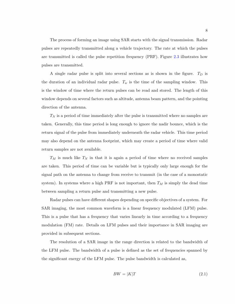
Radar pulses can have different shapes depending on specific objectives of a system. For

SAR imaging, the most common waveform is a linear frequency modulated (LFM) pulse.

This is a pulse that has a frequency that varies linearly in time according to a frequency

modulation (FM) rate. Details on LFM pulses and their importance in SAR imaging are

provided in subsequent sections.

The resolution of a SAR image in the range direction is related to the bandwidth of

the LFM pulse. The bandwidth of a pulse is defined as the set of frequencies spanned by

the significant energy of the LFM pulse. The pulse bandwidth is calculated as,

BW = |K|T (2.1)

9

-1

-0.5

0

0.5

1

LFM Pulses

TD

TN

Tw

TM

Fig. 2.3: Illustration of how radar pulses are transmitted according to a PRF.

where K is the FM rate and T is the total pulse duration

After calculating the pulse bandwidth, the range resolution can be shown to be ap-

proximately equal to

ρrng =c

2 ∗BW(2.2)

The resolution in the azimuth direction is not dependent on the LFM pulse like range

resolution. Instead, assuming the whole antenna azimuth swath has passed over the image

area in question, then the azimuth resolution is a function of the physical length of the

antenna, La.

ρazm =La2

(2.3)

Forming SAR images from received radar pulses is a process of matched filtering.

Collected data is processing through a matched filter in the range direction first, which

results in range compressed data. The range compressed data is then processed again in

the azimuth direction to form azimuth compressed data.

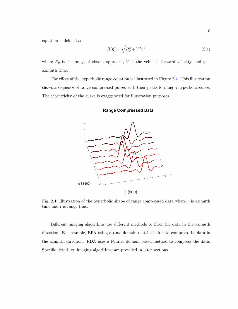
Compression in the azimuth direction is complicated by the fact that ground targets

appear as hyperbolic curves in the range compressed data. This can be explained by the

hyperbolic range equation, which is an expression for the instantaneous range between the

radar vehicle and a ground target at any point in time. Denoted R(η), the hyperbolic range

10

equation is defined as

R(η) =√R2

0 + V 2η2 (2.4)

where R0 is the range of closest approach, V is the vehicle’s forward velocity, and η is

azimuth time.

The effect of the hyperbolic range equation is illustrated in Figure 2.4. This illustration

shows a sequence of range compressed pulses with their peaks forming a hyperbolic curve.

The eccentricity of the curve is exaggerated for illustration purposes.

Fig. 2.4: Illustration of the hyperbolic shape of range compressed data where η is azimuthtime and t is range time.

Different imaging algorithms use different methods to filter the data in the azimuth

direction. For example, BPA using a time domain matched filter to compress the data in

the azimuth direction. RDA uses a Fourier domain based method to compress the data.

Specific details on imaging algorithms are provided in later sections.

11

CHAPTER 3

AN INVESTIGATION OF GPS-DENIED NAVIGATION USING AIRBORNE RADAR

TELEMETRY

A supplementary sensor being explored in the field of GPS-denied navigation is Syn-

thetic Aperture Radar (SAR) with its resulting images. In contrast to passive, camera-based

methods, SAR provides illumination of a scene, direct measurement of range, and can op-

erate day and night or through inclement weather. The research presented in this paper

investigates the feasibility of using range and range-rate measurements from a SAR system

to perform GPS-denied navigation. In support of this research, a 6DOF aircraft navigation

and radar simulation is developed and presented. The core sensor used to propagate the

navigation states is an inertial measurement unit, corrupted by bias and noise. An indi-

rect extended Kalman filter (EKF) is developed and the covariance of estimation errors is

validated via Monte Carlo analysis.

3.1 Introduction

GPS is a vital part of an INS. Without GPS, the system is forced to “Dead Reckon”,

which is to navigate without any external position update from GPS or radio link. Navigat-

ing without GPS is subject to drift and will result large inaccuracies over time. In situations

where GPS is unavailable or unreliable, a UAV must perform “GPS-denied Navigation”.

There are many examples that motivate GPS-denied navigation. In large cities, the

buildings form what is called an “Urban Canyon”. Because tall buildings obstruct the sky

and reflect incoming signals, GPS signals in urban canyons are unreliable and sometimes

unavailable. During military operations, GPS can be easily spoofed or jammed. These

and other such examples have motivated researchers to find efficient and reliable forms of

GPS-denied navigation.

Of the many different methods, one supplementary sensor being explored in GPS-denied

12

navigation is Synthetic Aperture Radar (SAR). SAR is a method of producing images of

an area using sequential radar pulses as an air/space craft flies along a given trajectory.

This project explores using range measurements and range-rate measurements from a radar

system in conjunction with an INS to estimate the trajectory of a UAV.

3.2 Literature Review

Historically, some major disadvantages of implementing a radar system are the size,

weight, and power requirements of the system. This would cause radar to be infeasible

for smaller UAVs; however, significant research has been performed to miniaturize radar

systems for UAV applications. Currently, flexible, light weight radar systems are available

commercially through IMST Radar that weigh as little as 164 grams [5].

GPS-denied navigation using radar can be split into two types: absolute navigation and

relative navigation. Absolute navigation finds the location of the UAV on a global coordinate

system, such as latitude, longitude, altitude. Relative navigation finds the location of the

UAV relative to some previously known location or target location.

Absolute navigation typically involves comparing collected data to an on-board terrain

map, elevation map, or satellite image. This kind of approach was performed by Nitti et al

in [6] using interferometric SAR. Greco et al used a similar method in [7].

Relative navigation does not try to determine an absolute position for the UAV, but

instead estimates the location of the UAV relative to the point where GPS was lost. This is

typically accomplished by associating radar data to prominent ground targets and tracking

those targets throughout the UAV’s trajectory. Scannapieco et al [8] performs this type of

navigation using a constant false alarm rate to detect prominent targets and then using a

global nearest neighbor approach to track targets.

In [9] and [10], Quist, Beard, and Niedfeldt detected and tracked targets using the

Hough transform. Unfortunately, the Hough transform is computationally expensive, which

is not feasible on some light UAV systems. In later papers, Quist et al proposed and tested

the Recursive RANSAC algorithm as a replacement of the Hough transform [11], [12].

13

Similar research has been performed by Kauffman et al using a method called Simultaneous

Localization and Mapping (SLAM) [13].

Radar data can be kept as either raw collected data, range compressed data, or fully

formed SAR images. Many of the absolute navigation methods use full SAR images in con-

junction with raw data and DTMs. Each type of data set has an associated computational

complexity, where raw data is the simplest form and fully formed images are the most com-

plex. To form a SAR image means filtering the raw data using matched filters. Filtering

once in the range dimension produces range compressed data. After range compression,

filtering in the azimuth dimension produces images [3].

To form high quality SAR images, the position of the aircraft at any given time must

be known with high accuracy. Errors in position will manifest themselves in the final

image as translations and blurrings of an imaged target. Research performed at Utah

State University has explored the effects of navigation errors on formed SAR images and

has explored methods of performing navigation based on the characteristics of the imaging

errors [14].

Several methods exist to form SAR images. One of the most computationally expen-

sive, but also one of the most accurate methods is the Back-Projection Algorithm (BPA).

The previously mentioned research at Utah State University was performed using BPA

SAR images to extract navigation errors. Other image formations with less computation

complexity exist, such as the Range-Doppler Algorithm (RDA). This algorithm sacrifices

image quality for a drastic reduction in computational complexity by using the FFT.

3.3 Method

This research could fall into the categories of either absolute or relative navigation,

depending on the knowledge of the target in the radar scene. To achieve GPS-denied

navigation, this research implements an INS and EKF system structure supplemented with

radar telemetry. Beginning with single point targets, necessary navigation data is extracted

from the radar data and processed within the EKF to produce estimates of the UAV state.

14

There exists an ambiguity between cross-track estimation errors and elevation estima-

tion errors. To help resolve the ambiguity, an additional altitude measurement is provided

to the EKF to help estimate the UAV state. This potential ambiguity exists due to sev-

eral different combinations of cross-track and elevation trajectory errors that could produce

an identical error pattern in the collected and processed radar data. This is illustrated

in Figure 3.1, which shows a continuum of cross-track and elevation positions that have a

constant range in relation to a target on the ground. This constant range to the target

leads to constant range of closest approach as extracted from radar telemetry for a given

target.

Fig. 3.1: Cross-track and elevation estimates are not unique given a slant range to target.

Measuring the altitude is most easily performed using an altimeter; however, this could

also be measured using a nadir bounce coupled with a Digital Terrain Elevation Data

(DTED) set. Using the nadir bounce and DTED does introduce another source of estimation

error, as now the UAV location in relation to the DTED must be known to get accurate

elevation data.

Figure 3.2 helps visualize the geometry of the UAV in relation to the target and how

15

it relates to radar telemetry. In the figure, the time varying range and the range of closest

approach are shown. The range measurement is equivalent to the time varying range in the

figure.

Fig. 3.2: Geometry of the UAV relative to the ground target.

Range to target, range-rate, and altitude measurements are combined in the EKF to

enable navigation independent of GPS. Once the INS and EKF structure is defined and val-

idated, further research will explore the effectiveness and sensitivity of the implementation.

This will be done by analyzing changes in results due to different grades of IMUs, different

types and levels of measurement noise, and different locations for radar ground targets.

3.4 State and Model Definitions

The EKF development begins by defining the truth state, estimated state, and error

state with their associated dynamics. Before defining state vectors and state models, co-

ordinate systems are defined. This research uses the flat earth model as a reference frame.

There are three coordinate systems of interest. These are: 1) The North-East-Down frame

(ned) with the origin attached to the body of the UAV, 2) The inertial frame (i) aligned

16

with the North-East-Down frame with its origin fixed on the Flat Earth model, and 3) The

body frame (b) attached to the body of the UAV with the x axis pointing out the nose of

the UAV, the y axis pointing out the right wing, and the z axis pointing out the belly of

the UAV.

With a defined coordinate system, state vectors and models can be defined. The

truth state vector is governed by the truth model, denoted x, the estimated state vector is

governed by the navigation model, denoted x, and the error state vector is governed by a

linear perturbation model, denoted δx.

The truth state and associated dynamics are defined as

x =

pned

vned

qnedb

baccel

bgyro

balt

brange

brate

=

vned

Rnedb νb + gned

qnedb ⊗ 12

[0ωb

]− 1τaccel

baccel + waccel

− 1τgyro

bgyro + wgyro

− 1τalt

balt + walt

− 1τrange

brange + wrange

− 1τrate

brate + wrate

(3.1)

where the elements of the state vector are respectively the position vector as expressed in

the ned frame, velocity vector as expressed in the ned frame, attitude quaternion between

the b and ned frames, accelerometer bias vector, gyroscope bias vector, altimeter bias, radar

range bias, and radar range-rate bias. Additionally, the ⊗ symbol represents quaternion

multiplication, Rnedb is the rotation matrix that rotates vectors from the UAV body frame

to the ned frame, νb is a measurement from the accelerometer, gned is the gravitational

constant, and ωb is a measurement from the gyroscope.

Note that each bias state is governed by a first order Markov model. Each Markov

model contains a time constant term ( 1τi

) and a process noise term (wi). There are Markov

models for the accelerometer bias, gyroscope bias, altimeter bias, radar range bias, and

17

range rate bias states.

The estimated state and navigation model are nearly identical to the truth state and

truth model apart from the velocity state and the attitude state. In the navigation model,

the velocity state and attitude state are propagated using measurements of specific force

and angular rate, compensated by the current estimate of the corresponding bias.

˙vned

qnedb

=

Rnedb(νb − baccel) + gned

qnedb⊗ 1

2

[0

ωb−bgyro

] (3.2)

Another key difference between the truth model and the navigation model is the ab-

sence of noise terms in the navigation model. The navigation model has no knowledge

of noise. Consequently, noise cannot be subtracted off of sensor measurements and bias

states. As such, the navigation model attempts to remove the bias from the accelerometer

and gyroscope measurements but cannot be completely successful.

It is important to clarify that νb and ωb are both truth measurements from the ac-

celerometer and gyroscope, respectively. An actual measurement from either instrument

will be corrupted by noise and bias. The resulting accelerometer measurement, νb, and

gyroscope measurement, ωb, are,

νb = νb + baccel + nν (3.3)

ωb = ωb + bgyro + nω (3.4)

where nν and nω are sensor noise vectors. Note the ˆ over each state variable and real

measurement. This notation is used throughout the paper and indicates an estimate.

The error state and perturbation model require more work to define. To do so, the

truth states are defined as a small perturbation from the estimated states. The truth model

is then expanded about the estimated state, after which the estimated state and nonlinear

terms are discarded. This results in a linear error model describing the dynamics of the

error state.

18

Because the error model is a linear model, it can be written in matrix notation in the

form

δx = F δx +Bw (3.5)

where F is defined as

F =

F11 F12

09×9 F22

(3.6)

where

F11 =

0 I 0

0 0 [Rnedb

(νb − baccel)]×

0 0 0

(3.7)

F21 =

0 0 0 0 0

−Rnedb

0 0 0 0

0 Rnedb

0 0 0

(3.8)

F22

− 1τaccel

I 0 0 0 0

0 − 1τgyro

I 0 0 0

0 0 − 1τalt

0 0

0 0 0 − 1τrange

0

0 0 0 0 − 1τrate

(3.9)

In equation 3.7, the “cross” operator, × is defined as

× : R3x1 → R3x3, s.t. (a×) =

[0 −a3 a2a3 0 −a1−a2 a1 0

]

where a = [a1, a2, a3]T .

B is defined as

B =

B11 09×9

09×9 I9×9

(3.10)

19

where

B11 =

0 0

−Rnedb

0

0 Rnedb

(3.11)

and w is the noise vector.

w = [nν ,nω,waccel,wgyro, walt, wrange, wrate]T (3.12)

3.5 Measurement Model

At each Kalman update time, measurements from the SAR image and altimeter must

be taken. Specifically, three measurements will be extracted from the data: Range to

target, range rate with respect to target, and altitude. For the purposes of this project, the

location of a given ground target is known. Knowledge of the target can be either global

(latitude-longitude) or relative (with respect to time of GPS loss).

The measurement functions can be constructed intuitively using Figure 3.3. In the

figure, r is the known position of a ground target in the inertial frame i as expressed in

the ned frame. pned is the position of the UAV in the i frame as expressed in the ned

frame. The range from the UAV to the target is the magnitude of the difference of the two

position vectors, ||r− pned||. The range rate is velocity of the aircraft, vned, projected into

the direction of r− pned.

There are two measurement models of importance. The first model is the measurement

taken from the onboard sensors denoted z. z is defined as

z =

zalt

zrange

zrate

=

−pz + balt + nalt

||r− pned||+ brange + nrange

−(vned)T r−pned||r−pned|| + brate + nrate

(3.13)

where n is measurement noise and pz is the down component of the position state.

For the purposes of this project, these measurements are synthesized using the truth

state vector of the UAV. In reality, these measurements would come from the SAR images

20

and altimeter. The second function is the estimated measurement denoted ˆz. This is the

value produced by propagation of the navigation model just before the Kalman update. ˆz

identical to z except that it is evaluated using the current estimated state rather than the

truth state.

Fig. 3.3: Geometry of range, range rate, and altitude measurements.

The measurement model must be linearized for processing in the EKF. This yields a

matrix H. This matrix H will be used in calculating the Kalman gain K and the updated

covariance value P+.

The linear measurement model is of the form

δz = Hδx +Gν (3.14)

where ν is a measurement noise vector.

ν = [nrange, nrate, nalt]T (3.15)

The matrix H is found by forming the Jacobian of the measurement model and evalu-

ating at x.

H =

[H1 03×9 I

](3.16)

21

where

H1 =

[0, 0,−1] 01×3

−dT||d|| 01×3

(vned)T

||d|| −(vned)TddT

||d||3−dT||d||

(3.17)

and where d = r− pned.

3.6 Covariance Propagation

The objective of this section is to develop the individual components of the error

state covariance propagation equation, where the error state covariance is denoted P . The

covariance propagation can be shown to be

P = FP + PF +BQBT (3.18)

where F and B are defined in Section 3.4.

The Q matrix in the covariance propagation equation is defined as the power spectral

density of the noise vector w defined in equation 3.12. Assuming each noise component is

zero mean, gaussian, and independent, Q is a diagonal equal to

Q = diag(σ2vrwI3×3, σ

2arwI3×3,

2σ2ss,baccel

τaccelI3×3,

2σ2ss,bgyro

τgyroI3×3,

2σ2ss,balt

τalt,2σ2

ss,brange

τrange,2σ2

ss,brate

τrate) (3.19)

3.7 Kalman Update

When a measurement is available to the EKF, a Kalman update is performed.

The equation for the Kalman gain is given by

K = P−HT (x−)[H(x−)P−HT (x−) +GRGT ]−1 (3.20)

where P− is the error state covariance before the Kalman update, H(x−) is the measure-

ment sensitivity matrix, G is the noise coupling matrix, and R is the covariance of the

22

measurement noise vector.

The error state covariance is updated using the Joseph form, which is given by

P+ = [I −KH(x−)]P−[I −KH(x−)]T +KGRGTKT (3.21)

The estimate of the error state is given by

δx+ = K[z− ˆz] (3.22)

After calculating an estimate of the error state vector, the estimate is applied to the

estimated state, which forms an updated estimated state vector. This is done using the

mapping,

x+ =

(pned)− + δpned

(vned)− + δvned[1

− 12δθnedb

]⊗ (qned

b)−

(baccel)− + δbaccel

(bgyro)− + δbgyro

(balt)− + δbalt

(brange)− + δbrange

(brate)− + δbrate

(3.23)

3.8 Filter Validation

This section validates the equations and definitions of the extended Kalman filter.

Before validation, an R matrix is selected, which determines the noise variances of the

radar and altimeter measurements. For this section, R is equal to

R =

σ2zrange

0 0

0 σ2zrate

0

0 0 σ2zalt

(3.24)

23

Fig. 3.4: Residual measurements after implementation of Kalman updates. From top tobottom: Altimeter residual, range residual, range-rate residual.

24

Fig. 3.5: Monte Carlo simulation with filtered covariance bounds. From top to bottom:North position east position, down position.

25

Fig. 3.6: Monte Carlo simulation with filtered covariance bounds. From top to bottom:North velocity east velocity, down velocity.

26

Fig. 3.7: Monte Carlo simulation with filtered covariance bounds. From top to bottom:North attitude east attitude, down attitude.

27

where the σzi are selected by the user and are defined in Table 3.1.

Table 3.1: Noise standard deviations used for SAR and altimeter measurement noises.

3σ (Measurement) Values

σzradar 0.2 (m)

σzrate 0.2 (m/s)

σzalt 0.2 (m)

If implemented correctly, the Kalman filter should produce residual measurements that

are zero-mean and white. After a single Monte Carlo run, the residual measurements with

their associated covariances are plotted. These plots are shown in Figure 3.4. In the figure,

the solid line represents the residual from a single Monte Carlo run and the dotted line

represents the 3σ bounds of the measurement residual.

It is observed that the measurement residuals satisfy the zero-mean and white condi-

tions. To further validate correct implementation of the Kalman update equations, a Monte

Carlo simulation with 200 runs is performed. Results of this validation are 3σ error state

covariance bounds that shrink as time goes on with each Kalman update. The results of

these tests are shown in Figures 3.5, 3.6, and 3.7.

After EKF implementation, the covariance of the estimation error diminishes. This

further implies correct definition and implementation of the Kalman update equations.

3.9 Results

This section documents the studies and contributions performed by this project. Three

separate studies were performed. One on the sensitivity of estimation errors to changes in

IMU grade. The second on the sensitivity to measurement noise strength. The third on the

sensitivity to the geometric relationship between the platform and target is studied.

3.9.1 Sensitivity to IMU Grade

To test the sensitivity of the INS to IMU grade, a single iteration of the Monte-Carlo

simulation is run with noise typical of consumer grade, tactical grade, and navigation grade

28

IMUs.

Table 3.2 shows the different parameters chosen for the IMU grade study. Values in

the table are reported as 3σ values. In the table, note that vrw and arw stand for velocity

random walk and angular random walk, respectively.

Table 3.2: Different IMU grades used in investigation expressed as 3σ values.

IMU Grade σ3s,vrw σ3s,accel σ3s,arw σ3s,gyro

Consumer 0.6 0.01 0.7 10

Tactical 0.06 0.001 0.07 1

Navigation 0.006 0.0001 0.007 0.1

The results of the study are shown in Figure 3.8. The three plots shown show the

north, east, and down position estimation errors expressed as 3σ covariance bounds.

Improvements in state estimates are evident with each IMU upgrade, but the difference

between navigation grade and tactical grade is much smaller than the difference between

tactical grade and consumer grade. This is most evident in the north and east position

states. Down position states are less affected by IMU grade because of available direct

altitude measurements from the altimeter.

3.9.2 Sensitivity to SAR Measurement Noise

This section studies the effects of different measurement noise variances on the accuracy

of the state estimations. Table 3.3 shows the different measurement noise strengths used

for each test in this study. The measurement noise strengths are expressed in the table as

3σ values. The noise strength is changed one measurement at a time in order to isolate how

the uncertainty of a single measurement affects the state estimations.

As in the IMU grade study, plots of position estimation error covariance bounds are

given. These plots are shown in Figure 3.9

The figure shows that altimeter measurement noise strongly affects the down position

and down velocity state estimates. Range-rate and range measurement noise affected the

north and east positions but had little effect on the down position.

29

Table 3.3: Levels of measurement noise used in investigation expressed as 3σ values.

Test # σ3s,nrange (m) σ3s,nrate (m/s) σ3s,nalt (m)

1 0.2 0.2 0.2

2 2 0.2 0.2

3 0.2 2 0.2

4 0.2 0.2 2

3.9.3 Sensitivity to Platform/Target Geometry

This section studies how the positioning of the ground target affects state estimation.

Table 3.4 lists the different locations of the ground target in the local cartesian coordinate

system. Note that in the local coordinate system, the flight trajectory begins as the point

[0, -200, 0] and travels directly north.

Table 3.4: Different locations of the ground target relative to the flight trajectory used ininvestigation.

Test # rn (m) re (m) rd (m)

1 500 0 0

2 500 500 0

3 500 1000 0

4 500 1500 0

5 1000 0 0

6 1000 500 0

7 1000 1000 0

8 1000 1500 0

Results of this study are shown in Figures 3.10 and 3.11. Each of the plots in the

figure are of the same format as previous studies. That is to say that each plot shows 3σ

covariance bounds of the position estimation error. For this study, only north and east

position estimation errors are shown, because altitude errors are invariant to ground target

location due to the availability of altitude measurements.

The location of the ground target dramatically affects the convergence rates of the

north and east state estimates. Convergence behavior improves as the ground target grows

closer to the flight trajectory and as the ground target moves closer to the beginning of the

flight trajectory.

30

3.10 Conclusion

This research studies the estimation performance of an INS aided by an altimeter and

radar telemetry. Radar measurements are derived from range and range rate to ground

targets. The studies performed explored how noise strength, measurement fidelity, and

target location affect state estimation error.

The simulation results suggest that GPS-denied navigation using radar telemetry is

most feasible when using either a tactical or navigation grade IMU and when using a SAR

system with high fidelity range measurements. The simulation also demonstrates that

the location of the ground target significantly influences estimation performance. Overall,

targets close to the flight trajectory yielded better estimation performance. The results

further suggest that no substantial benefit is achieved when upgrading from tactical to

navigation grade, which motivates the use of the tactical grade IMU.

In general, the estimates with the most error were the north and east position estimates.

Down position estimates were small due to the presence of altimeter measurements.

3.11 Acknowledgments

This research was funded in part by Sandia National Laboratories, whom we thank.

31

Fig. 3.8: Position estimation errors expressed as covariance bounds to illustrate IMU gradedifferences. From top to bottom: North position, east position, down position. By line type:Dashed line represents consumer grade, solid line represents tactical grade, and dot-dashline represents navigation grade.

32

Fig. 3.9: Position estimation errors expressed as covariance bounds to illustrate measure-ment error differences. From top to bottom: North position, east position, down position.By line type: Dashed line represents increased range error, dot-dash line represents increasedrange-rate error, dotted line represents increased altitude error, and solid line represents noincreased error.

33

Fig. 3.10: Position estimation errors expressed as covariance bounds to illustrate groundtarget placement. From right to left: North position, east position. Line types: Dashedline for target at (500, 0, 0), dot-dash line for target at (500, 500, 0), solid line for targetat (500, 1000, 0), and dotted line for target at (500, 1500, 0).

Fig. 3.11: Position estimation errors expressed as covariance bounds to illustrate groundtarget placement. From right to left: North position, east position. Line types: Dashedline for target at (1000, 0, 0), dot-dash line for target at (1000, 500, 0), solid line for targetat (1000, 1000, 0), and dotted line for target at (1000, 1500, 0).

34

CHAPTER 4

SENSITIVITY OF BPA SAR IMAGE FORMATION TO INITIAL POSITION,

VELOCITY, AND ATTITUDE NAVIGATION ERRORS

The Back-Projection Algorithm (BPA) is a time domain matched filtering technique

to form synthetic aperture radar (SAR) images. To produce high quality BPA images,

precise navigation data for the radar platform must be known. Any error in position,

velocity, or attitude results in improperly formed images corrupted by shifting, blurring,

and distortion. This paper develops analytical expressions that characterize the relationship

between navigation errors and image formation errors. These analytical expressions are

verified via simulated image formation and real data image formation.

4.1 Introduction

Synthetic aperture radar (SAR) is a class of radar processing that uses the flight path

of a spacecraft or aircraft, referred to as a radar platform, to create a synthetic imaging

aperture. Through a collection of matched filters, raw radar data is processed into images.

Many efficient matched filtering algorithms have been developed that employ the frequency

domain, such as the range-Doppler algorithm, the chirp scaling algorithm, the omega-K

algorithm, and more [3]. Time domain algorithms also exist, such as the Back-Projection

Algorithm (BPA) [15].

This paper explores the sensitivity of BPA images to navigation errors. This is done

first analytically using the range equation and back-projection equation, which are both

defined in Section 4.2. Secondly the analysis is verified by injecting error into a flight

trajectory estimate of an aircraft and using the corrupted trajectory estimate to form BPA

images. This process is performed on both simulated and real data.

35

4.1.1 Motivation

The research in this paper is primarily motivated by the field of GPS denied navigation

but may be of interest to other fields relating to SAR image quality or image autofocusing.

GPS denied navigation is a field of research that involves estimating the state of a vehicle in

the absence of Global Navigation Satellite Systems (GNSS) such as GPS. Typical approaches

utilize an inertial navigation system (INS) as the core sensor, aided by measurements from

auxiliary sensors, in the framework of an extended Kalman filter. Such auxiliary sensors

may include cameras, lidar, radar, etc, [16].

When forming a SAR image using back-projection, navigation data and raw radar data

are processed to form an image. Obtaining precise navigation data in an ideal application

requires the use of GPS. However, in a GPS denied environment, navigation errors may be

present, which result in distorted SAR images. This research is motivated by the potential

of inferring navigation errors from induced image errors during BPA image formation [17].

This paper works toward building the foundation and intuition needed to achieve such a

potential.

4.1.2 Literature Review

BPA is more sensitive to navigation errors than other types of SAR image formation

techniques. This can be inferred from Duersch and Long who explore some of the sensi-

tivities inherent in forming images using back-projection [15]. This research expands the

sensitivity analysis to motion errors as seen from a navigation point of view with a more

complete navigation state.

BPA is essentially a matched filter along a hyperbolic curve within a set of range

compressed data. Integrating along a curve requires that each data sample be precisely

selected in correspondence with the current position of the vehicle. Any error in navigation

data results in integrating data on an incorrect curve with an incorrect phase. Very precise

navigation data is therefore necessary to form accurate BPA images [15]. Further details

on BPA are discussed in Section 4.2.

Errors in navigation data manifest themselves in a SAR image as shifts and distortions

36

of a given target. Research performed by Christensen et al explores the effects of navi-

gation errors on fully formed SAR images and hypothesizes that navigation errors can be

determined by comparing degraded SAR images to a reference SAR map [17].

Many types of errors can affect the quality of SAR images. As such a comprehensive

analysis of image errors is difficult and requires further investigation. Current efforts in

analyzing image errors include research performed by Bamler [18] and Farrel et al [19]. They

explore image errors caused by servo transients, quantization, range uncertainty, range-rate

uncertainty, and focusing algorithm selection. Additionally, Chen explores image errors

caused by moving targets in the illuminated scene [20].

In previous literature, navigation errors have been expressed as range displacement,

line of sight displacement, and forward velocity error. Moreira and Xing et al adjust the

SAR pulse repetition frequency (PRF) to compensate for forward velocity errors [21], [22].

Moreira further adjusts phase and range delays to compensate for line of sight displacement

errors. Velocity errors in particular have been shown to affect the Doppler parameters

of the SAR data, which cause target location errors and image degradation in the final

image [22], [23].

4.1.3 Contributions

A comprehensive study of BPA SAR image errors in the context of the full navigation

state has not been performed to date. The research seeks to fill this void by developing

relationships between image shifts, blurs, and distortions and all components of navigation

state, specifically position, velocity, and attitude errors.

Section 4.2 begins by providing necessary background knowledge concerning inertial

navigation and BPA processing. Section 4.3 develops the math necessary to predict how

navigation errors affect the final SAR image. Sections 4.4 and 4.5 demonstrate the appli-

cation of the error analysis to simulated and real data, respectively. Section 4.6 provides

concluding discussion and summary.

4.2 Background

37

4.2.1 Inertial Navigation

The purpose of this section is to define an inertial navigation framework applicable to

the short data collection times typical of SAR imagery. The framework is then used to

develop analytical expressions of position estimation error growth.

Inertial navigation is a large field with an equally-large body of literature dating back

to the 1930’s. An excellent overview of the history and motivating factors behind the

development of this field is provided in [24]. The navigation framework developed in this

section utilizes concepts discussed in [24–26]. The developed framework is most directly

related to the so-called “Tangent Frame” kinematic model [25], with the assumptions of

constant gravity and a non-rotating earth, both of which are applicable over the short time

frame typical of an airborne SAR data collection. In the development that follows, the truth

and navigation states are defined, with the associated differential equations. Consistent with

an extended Kalman filter framework, the truth state differential equations are linearized

about the estimated navigation state to derive the differential equations of the estimation

errors, or error states.

The truth state vector comprises the true position (pn), velocity (vn), and attitude

quaternion (qnb ) of the vehicle

x =

[pn vn qnb

]T(4.1)

where n and b refer to the navigation and body frame, respectively. The body frame origin

is coincident with the navigation center of the inertial measurement unit (IMU), with the

axes aligned and rotating with the vehicle body axes. Out of convenience for the subsequent

analysis, and without loss of generality, the navigation frame is defined with the x-axis

parallel to the velocity of the vehicle, the z-axis in the direction of gravity, and the y-axis

defined by the right-hand-rule. The x, y, and z axes, therefore, correspond to the along-

track, cross-track, and down directions typical of radar imaging conventions. Consistent

with Ferell’s definition of the “Tangent Frame” [25], the position and velocity are defined

relative to a fixed origin, whose location is the position of the vehicle at the beginning of the

38

SAR data collection. The differential equations of the truth states are defined as follows1

pn

vn

qnb

=

vn

Tnb νb + gn

12qnb ⊗

0

ωb

(4.2)

The strapdown inertial navigation system comprises a three-axis accelerometer and gyro,

which provide measurements of specific force(νb)

and angular rate(ωb)

in the body frame,

corrupted by noise νb

ωb

=

νb

ωb

+

nν

nω

(4.3)

The navigation states are defined identical to the truth states but are propagated using

noisy accelerometer and gyro measurements

˙pn

˙vn

˙qnb

=

vn

Tnb νb + gn

12 qnb ⊗

0

ωb

(4.4)

The estimation error, or error state vector,

δx =

[δpn δvn δθn

]T(4.5)

is defined as the difference between the truth states and the navigation states. For all

but the attitude states, the difference is defined by a simple subtraction. For the attitude

quaternion the difference is defined by a quaternion product.

δpn = pn − pn (4.6)

1In this work, the quaternion is interpreted as a “left-handed” quaternion, and the ⊗ operator is theHamiltonian quaternion product [27].

39

δvn = vn − vn (4.7) 1

−12δθ

n

= qnb ⊗ (qnb )∗ (4.8)

It is also convenient to define the attitude errors in terms of the true and estimated trans-

formation matrices

[I − (δθn×)] = Tnb

(Tnb

)T(4.9)

Linearization of (4.2) about the estimated state results in the error state differential equation

δx = Fδx+Bw (4.10)

where the state dynamics matrix, F , and noise coupling matrix, B, are defined respectively

as

F =

03×3 I3×3 03×3

03×3 03×3

[Tnb ν

b]×

03×3 03×3 03×3

(4.11)

B =

03×3 03×3

−Tnb 03×3

03×3 Tnb

(4.12)

and where the white noise (w) consists of the accelerometer and gyro measurement noise

w =

[nν nω

]T(4.13)

The focus of this paper is to analyze the sensitivity of the BPA image to errors in position,

velocity, and attitude at the beginning of the synthetic aperture. The effect of w is therefore

ignored, and the analysis is facilitated by determining the homogenous solution to (4.10)

δxk = Φ (tk, tk−1) δxk−1 (4.14)

40

where Φ (tk, tk−1) is the state transition matrix (STM) from the tk−1 to tk. The STM is

defined as the matrix which satisfies the differential equation and initial condition

Φ (tk+1, tk) = F (t) Φ (tk+1, tk) (4.15)

Φ (tk, tk) = In×n (4.16)

For the case of straight-and-level flight, the dynamic coupling matrix of (4.11) is constant,

F =

03×3 I3×3 03×3

03×3 03×3 (νn)×

03×3 03×3 03×3

(4.17)

Where the accelerometer measurements are expressed in the n frame as

νn =

[0 0 −g

]T(4.18)

Since F is constant, the STM is derived using the matrix exponential ( [4], page 42)

Φ (tk+1, tk) =

I3×3 I3×3∆t (νn×) ∆t2

2!

03×3 I3×3 (νn)×∆t

03×3 03×3 I3×3

(4.19)

The desired analytical expression for position errors is obtained from the first row of

the STM to yield

δpn (t) = δpn0 + δvn0 ∆t+ νn × δθn0∆t2

2(4.20)

In all subsequent sections, the variables representing positions, velocities, and attitudes

are all assumed to be in the n frame. As such, the n superscript on all navigation states is

omitted for notational brevity.

41

4.2.2 Back-Projection Algorithm

Forming images using SAR is a process of matched filtering that transformed raw re-

turned radar signals into focused pixels. A raw SAR signal is typically a linear frequency

modulated (FM), or “chirp”, signal. Chirp signals are a sinusoid-like signal with an instan-

taneous frequency that is linear with time. A transmitted chirp signal is denoted stx(t) and

is equal to

stx(t) =

exp(j2πf0t+ jπKt2), 0 ≤ t ≤ T

0, otherwise

(4.21)

where f0 is the initial frequency, K is the linear FM rate in hertz per second, and T is the

pulse duration.

The chirp signal is transmitted several times along the trajectory, and return signals

are collected for each transmitted signal. Using a “stop and hop” approximation, the return

radar signal is a time shifted, attenuated version of the transmitted signal given by

srx(t) = Astx(t− τ) (4.22)

The return signal is fed through a matched filter in a process called “range compres-

sion”. The matched filter is a time reversed, conjugate version of the transmitted signal

stx(t). The output of the matched filter is denoted sout(t) and is equal to the convolution

of srx(t) with s∗tx(T − t).

sout(t) = srx(t) ∗ s∗tx(T − t) (4.23)

=

∫ t

0 srx(λ)s∗tx(T − (t− λ))dλ, 0≤t≤ T∫ Tt−T srx(λ)s∗tx(T − (t− λ))dλ, T ≤t≤2T

Evaluating the convolution results in

42

sout(t) = e−jρ(2πf0+πKT )

sin(πKρt)πKρ , 0≤t< T

T, t = T

sin(πKρ(2T−t))πKρ , T <t≤2T

(4.24)

where ρ = T−t. This expression can be written in a closed form using the sinc function

sinc(x) = sin(πx)/πx.

sout(t) = e−jρ(2πf0+πKT )ξsinc(Kρξ) (4.25)

where ξ is equal to T − |t− T |.

After range compression, the sequential returns from a single target form a hyperbolic

curve in the range compressed data. This hyperbola is quantified via the range equation

denoted R(pt, η) and defined as

R(pt, η) = ‖pt − p(η)‖ (4.26)

where pt is the position of a target of the ground and p is the true time-varying position of

the aircraft from (4.1). The aircraft position varies with azimuth time (or slow time), η.

To form an image using BPA, a second matched filter is applied to the range compressed

data in the azimuth direction. This is called “azimuth compression”. Azimuth compression

using BPA is performed in the time domain and is dependent on the range equation, which

is dependent on the position of the radar vehicle. For a particular pixel location, ppix,

azimuth compression is defined by the summation,

A(ppix) =∑k

sout(tpix,k)exp

{j4π

Rk(ppix, η)

λ

}(4.27)

where k is used to denote the kth range compressed signal, λ is the wavelength at the center

frequency of the chirp signal, and tpix,k is the time during the kth range compressed signal

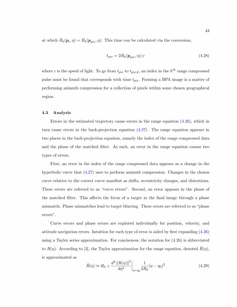
43

at which Rk(pt, η) = Rk(ppix, η). This time can be calculated via the conversion,

tpix = 2Rk(ppix, η)/c (4.28)

where c is the speed of light. To go from tpix to tpix,k, an index in the kth range compressed

pulse must be found that corresponds with time tpix. Forming a BPA image is a matter of

performing azimuth compression for a collection of pixels within some chosen geographical

region.

4.3 Analysis

Errors in the estimated trajectory cause errors in the range equation (4.26), which in

turn cause errors in the back-projection equation (4.27). The range equation appears in

two places in the back-projection equation, namely the index of the range compressed data

and the phase of the matched filter. As such, an error in the range equation causes two

types of errors.

First, an error in the index of the range compressed data appears as a change in the

hyperbolic curve that (4.27) uses to perform azimuth compression. Changes in the chosen

curve relative to the correct curve manifest as shifts, eccentricity changes, and distortions.

These errors are referred to as “curve errors”. Second, an error appears in the phase of

the matched filter. This affects the focus of a target in the final image through a phase

mismatch. Phase mismatches lead to target blurring. These errors are referred to as “phase

errors”.

Curve errors and phase errors are explored individually for position, velocity, and

attitude navigation errors. Intuition for each type of error is aided by first expanding (4.26)

using a Taylor series approximation. For conciseness, the notation for (4.26) is abbreviated

to R(η). According to [3], the Taylor approximation for the range equation, denoted R(η),

is approximated as

R(η) ≈ R0 +d2 ‖R(η)‖2

dη2

∣∣∣∣η=η0

1

2R0(η − η0)2 (4.29)

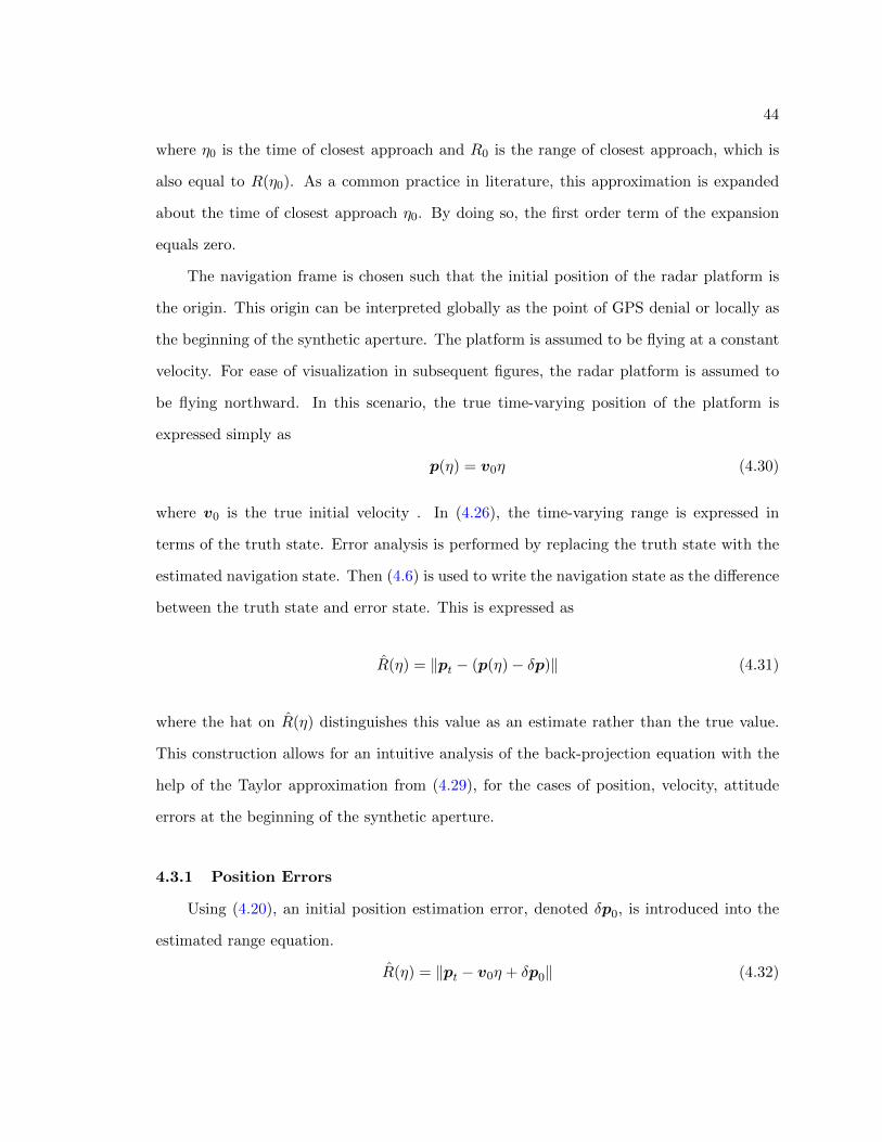
44

where η0 is the time of closest approach and R0 is the range of closest approach, which is

also equal to R(η0). As a common practice in literature, this approximation is expanded

about the time of closest approach η0. By doing so, the first order term of the expansion

equals zero.

The navigation frame is chosen such that the initial position of the radar platform is

the origin. This origin can be interpreted globally as the point of GPS denial or locally as

the beginning of the synthetic aperture. The platform is assumed to be flying at a constant

velocity. For ease of visualization in subsequent figures, the radar platform is assumed to

be flying northward. In this scenario, the true time-varying position of the platform is

expressed simply as

p(η) = v0η (4.30)

where v0 is the true initial velocity . In (4.26), the time-varying range is expressed in

terms of the truth state. Error analysis is performed by replacing the truth state with the

estimated navigation state. Then (4.6) is used to write the navigation state as the difference

between the truth state and error state. This is expressed as

R(η) = ‖pt − (p(η)− δp)‖ (4.31)

where the hat on R(η) distinguishes this value as an estimate rather than the true value.

This construction allows for an intuitive analysis of the back-projection equation with the

help of the Taylor approximation from (4.29), for the cases of position, velocity, attitude

errors at the beginning of the synthetic aperture.

4.3.1 Position Errors

Using (4.20), an initial position estimation error, denoted δp0, is introduced into the

estimated range equation.

R(η) = ‖pt − v0η + δp0‖ (4.32)

45

This equation is then expanded using the Taylor approximation, again denoted with a

tilde.

ˆR(η) = ‖pt − v0η0 + δp0‖ (4.33)

+(v0)Tv0

2 ‖pt − v0η0 + δp0‖(η − η0)2

In the first term of the expansion, δp0 causes a constant shift of the hyperbola used

for azimuth compression. In the second term, δp0 in the denominator is typically small

compared pt − v0η0. As such, its contribution to the overall error is very small and can

be ignored. In terms of curve errors, the estimated hyperbola is shifted in the direction of

δp0 due to the first term of the expansion. For phase errors, constant offsets do not affect

the overall focus of any imaged target [3]. Phase offsets only affect knowledge of absolute

phase.

The notional effects of position errors are illustrated in Figures 4.1, 4.2, and 4.3. Each

figure is split into three subfigures showing how a position error propagates through different

stages of radar processing. The first subfigure shows the error’s effect on the flight trajectory.

The second subfigure shows the error’s effect on the range compressed data. The third

subfigure shows the error’s effect on the final image.

In each figure, light colored or dotted illustrations represent expected data given es-

timation errors. Solid black illustrations represent actual data given no estimation errors.

These figures primarily provide intuition primarily on curve errors but can be useful in

visualizing phase errors as well.

4.3.2 Velocity Errors

From (4.20), an initial velocity estimation error is introduced into the estimated range

equation as

R(η) = ‖pt − (v0 − δv0)η‖ (4.34)

46

Fig. 4.1: Illustration of how cross track position errors affect the various stages of radarprocessing. Left: flight trajectory with error. Center: range compressed data with error.Right: final image with error. Light colored or dotted illustrations represent expected datagiven estimation errors. Solid black illustrations represent truth data.

Fig. 4.2: Illustration of how along track position errors affect the various stages of radarprocessing. Left: flight trajectory with error. Center: range compressed data with error.Right: final image with error. Light colored or dotted illustrations represent expected datagiven estimation errors. Solid black illustrations represent truth data.

Fig. 4.3: Illustration of how elevation position errors affect the various stages of radarprocessing. Left: flight trajectory with error. Center: range compressed data with error.Right: final image with error. Light colored or dotted illustrations represent expected datagiven estimation errors. Solid black illustrations represent truth data.

47

Fig. 4.4: Illustration of how cross track velocity errors affect the various stages of radarprocessing. Left: flight trajectory with error. Center: range compressed data with error.Right: final image with error. Light colored or dotted illustrations represent expected datagiven estimation errors. Solid black illustrations represent truth data.

Fig. 4.5: Illustration of how along track velocity errors affect the various stages of radarprocessing. Left: flight trajectory with error. Center: range compressed data with error.Right: final image with error. Light colored or dotted illustrations represent expected datagiven estimation errors. Solid black illustrations represent truth data.

Fig. 4.6: Illustration of how elevation velocity errors affect the various stages of radarprocessing. Left: flight trajectory with error. Center: range compressed data with error.Right: final image with error. Light colored or dotted illustrations represent expected datagiven estimation errors. Solid black illustrations represent truth data.

48

Fig. 4.7: Progression of roll errors through the SAR data. Left: flight trajectory witherror. Center: range compressed data with error. Right: final image with error. Lightcolored or dotted illustrations represent expected data given estimation errors. Solid blackillustrations represent truth data.

Fig. 4.8: Progression of pitch error through the SAR data. Left: flight trajectory witherror. Center: range compressed data with error. Right: final image with error. Lightcolored or dotted illustrations represent expected data given estimation errors. Solid blackillustrations represent truth data.

49

Again, the Taylor expansion is taken and results in

ˆR(η) = ‖pt − (v0 − δv0)η0‖ (4.35)

+(v0)Tv0 − 2(v0)T δv0 + (δv0)T δv0

‖pt − (v0 − δv0)η0‖(η − η0)2

In the first term of the expansion, there is again a constant offset due to δv0. As

is the case for initial position errors, this constant offset causes a shifted curve error and

a negligible offset phase error. In the second term of the expansion, (δv0)T δv0 in the

numerator is a quadratic error term and contribute little overall error. Similar to the case

of position errors, the δv0η term in the denominator contributes negligible overall error due

to its relative size compared to the rest of the denominator.

In the numerator of the second term, 2(v0)T δv0 causes a time-varying error. In terms of

curve errors, this changes the eccentricity of the expected hyperbola in the range compressed

data. For phase errors, this term can be thought of a linearly changing frequency error or

azimuth FM rate error.

An azimuth FM rate error is characterized by a phase that changes quadratically in

time. A quadratically varying phase yields a linearly changing instantaneous frequency.

This is similar to the linear FM signal modeled by equation (4.21). For both curve errors

and phase errors, the second numerator term results in blurring of the imaged target in

the azimuth dimension. This blur is only present in along track errors, as cross track and

elevation errors result in a δv0 that is orthogonal to v0.

Again, the notional effects are illustrated in Figures 4.4, 4.5, and 4.6 for various stages of

SAR processing. Each figure is again split into three subfigures with identical interpretations

as Figures 4.1, 4.2, and 4.3.

4.3.3 Attitude Errors

Again using (4.20), initial attitude errors are injected into the range equation to yield

R(η) =

∥∥∥∥pt − v0η + νn × δθ0η2

2

∥∥∥∥ (4.36)

50

Errors in attitude manifest as errors in acceleration. Specific effects from attitude errors are

apparent after computing the cross product. Using constant accelerometer measurements,

νn × δθ0 =

0

0

−g

×δθx,0

δθy,0

δθz,0

=

δθy,0g

−δθx,0g

0

(4.37)

This equation illustrates how attitude errors only cause acceleration errors in the along track

and cross track directions. Specifically, errors in roll, δθx,0, cause cross track acceleration

errors. Errors in pitch, δθy,0, cause along track acceleration errors. Errors in yaw do not

cause any errors in acceleration.

For conciseness, acceleration errors resulting from (4.37) are collectively referred to as

δv0. As such, the estimated range equation takes the form

R(η) =

∥∥∥∥pt − v0η +1

2δv0η

2

∥∥∥∥ (4.38)

The effects of acceleration errors are again explored using the Taylor approximation of

the estimated range equation.

ˆR(η) =

∥∥∥∥pt − v0η0 +1

2δv0η

20

∥∥∥∥ (4.39)

+Q∥∥pt − v0η0 + 1

2δv0η20

∥∥(η − η0)2

where

Q =1.5(δv0)T δv0η20 − 3(δv0)Tv0η0 (4.40)

+ pTt δv0 + (v0)Tv0

In the first term of the expansion, 12δv0η

20 causes a constant offset. For curve errors, this

term causes a small shift in the imaged target. In practice, this shift isn’t strongly apparent,

because the image degrades due to other terms before the shifting becomes strong. For phase

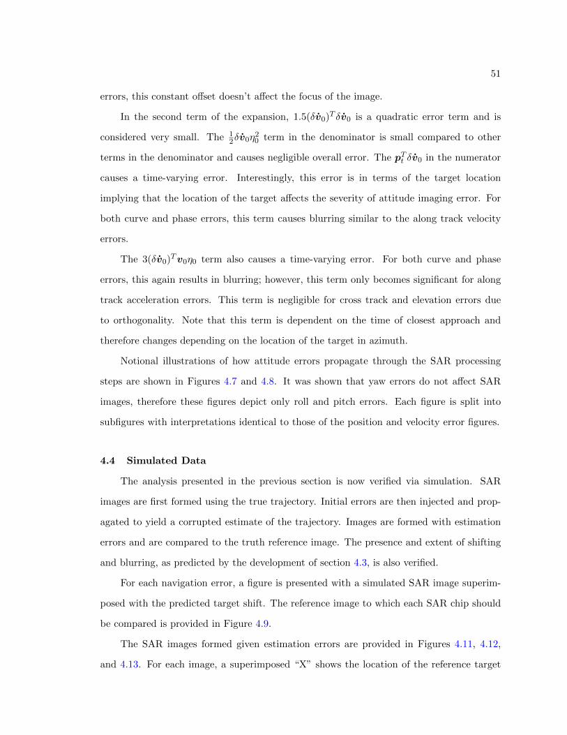
51

errors, this constant offset doesn’t affect the focus of the image.

In the second term of the expansion, 1.5(δv0)T δv0 is a quadratic error term and is

considered very small. The 12δv0η

20 term in the denominator is small compared to other

terms in the denominator and causes negligible overall error. The pTt δv0 in the numerator

causes a time-varying error. Interestingly, this error is in terms of the target location

implying that the location of the target affects the severity of attitude imaging error. For

both curve and phase errors, this term causes blurring similar to the along track velocity

errors.

The 3(δv0)Tv0η0 term also causes a time-varying error. For both curve and phase

errors, this again results in blurring; however, this term only becomes significant for along

track acceleration errors. This term is negligible for cross track and elevation errors due

to orthogonality. Note that this term is dependent on the time of closest approach and

therefore changes depending on the location of the target in azimuth.

Notional illustrations of how attitude errors propagate through the SAR processing

steps are shown in Figures 4.7 and 4.8. It was shown that yaw errors do not affect SAR

images, therefore these figures depict only roll and pitch errors. Each figure is split into

subfigures with interpretations identical to those of the position and velocity error figures.

4.4 Simulated Data

The analysis presented in the previous section is now verified via simulation. SAR

images are first formed using the true trajectory. Initial errors are then injected and prop-

agated to yield a corrupted estimate of the trajectory. Images are formed with estimation

errors and are compared to the truth reference image. The presence and extent of shifting

and blurring, as predicted by the development of section 4.3, is also verified.

For each navigation error, a figure is presented with a simulated SAR image superim-

posed with the predicted target shift. The reference image to which each SAR chip should

be compared is provided in Figure 4.9.

The SAR images formed given estimation errors are provided in Figures 4.11, 4.12,

and 4.13. For each image, a superimposed “X” shows the location of the reference target

52

Reference Image

596 598 600 602 604

ground range (m)

446

448

450

452

454

azim

uth

(m

)

Fig. 4.9: Reference image for simulated SAR data.

in relation to the current image. A superimposed “O” shows the predicted location of the

target given the injected estimation errors.

The “X” and “O” are generated using the true range equation, (4.26), and the estimated

range equation, (4.31), respectively. Equation (4.26) is used to find the true range of closest

approach and time of closest approach, denoted R0 and η0. Equation (4.31) is used to find

the estimated range of closest approach and time of closest approach, denoted R0 and η0.

R0 = minR(η), R0 = min R(η) (4.41)

η0 = arg minη

R(η), η0 = arg minη

R(η)

The range of closest approach and time of closest approach are used as coordinates to

overlay “X” and “O” onto each image.

Figures 4.11-4.13 illustrate that in all cases, the direction of shifts and blurs is consistent

with the development of section 4.3. Furthermore, in cases where blur is negligible, the

amount of shift is accurately predicted utilizing the method described previously. It is

important to highlight the ambiguity that exists in relating the SAR image error with the

attributing navigation error. From a single image, for example, it is impossible isolate the

effects of cross track position and elevation errors, since both cause shifts in the cross track

53

position of the target. Similar difficulties existing in attributing along-track shifts and blurs

to the corresponding navigation errors.

4.5 Real Data

The analysis from Section 4.3 is be further verified using real SAR data. Radar data

was collected in Logan, Utah. SAR images are formed using a post-processed, high fidelity

navigation solution, which is considered truth for the purposes of this research. The ref-

erence image in Figure 4.10 is formed using the truth trajectory. Each type of navigation

error is then injected into the truth trajectory, from which the distorted SAR images of

Figures 4.14-4.16 are formed.

Reference Image

20 40 60 80

ground range (pix)

20

40

60

80

azim

uth

(pix

)

Fig. 4.10: Reference image for real SAR data.

The results on real SAR data mirror the trends observed in section 4.4. The type and

direction of the shifts and blurs are consistent with the predictions of section 4.3. In the

case of negligible blurs, the shifts on real data are accurately predicted using the method

described in section 4.4 for all cases except yaw error, where a very small prediction error is

observed. Finally, ambiguity in the attribution of error sources to image errors is observed

in the real SAR data. Despite the small discrepancy in yaw, these results serve to further

validate the relationships developed in section 4.3.

54

4.6 Conclusion

This paper analyzes errors in the formation of SAR images using the Back-Projection

Algorithm from a navigation perspective, for the case of straight-and-level flight. Relation-

ships are developed between the position, velocity, and attitude estimation errors at the

beginning of the synthetic aperture and the observed shifts and blurs of the corrupted BPA

SAR image.

The developed relationships were observed and validated on both simulated and real

SAR data. In the case of negligible blurring, the location of the target in the corrupted SAR

image is accurately predicted given knowledge of the attributing navigation error. These

results suggest that errors in BPA SAR images could potentially be used in reverse, i.e.

image errors could be characterized and exploited as a navigation aid in GPS-denied appli-

cations. For a single image, however, it was observed that the shifts/blurs are not unique

to an individual navigation error. The presence of the target location in the developed

relationships suggests that the effect of navigation errors can be modified by the selection

of the target location. One obvious extension of this work is the consideration of multiple

targets with large geometric diversity, to resolve the ambiguity in attributing error sources.

Furthermore, methods which characterize the amount and direction of image blurring must

be developed to exploit the information contained therein.

55

Along Track Pos Errors

596 598 600 602 604

ground range (m)

446

448

450

452

454

azim

uth

(m

)

Cross Track Pos Errors

596 598 600 602 604

ground range (m)

446

448

450

452

454

azim

uth

(m

)

Elevation Pos Errors

596 598 600 602 604

ground range (m)

446

448

450

452

454

azim

uth

(m

)

Fig. 4.11: Position errors in simulated data: Top, along track position error (3 m). Middle,cross track position error (3 m). Bottom, elevation position error (3 m). Each figure issuperimposed with a reference target location, “X”, and a predicted target shift, “O”.

56

Along Track Vel Errors

596 598 600 602 604

ground range (m)

446

448

450

452

454

azim

uth

(m

)

Cross Track Vel Errors

596 598 600 602 604

ground range (m)

446

448

450

452

454

azim

uth

(m

)

Elevation Vel Errors

596 598 600 602 604

ground range (m)

446

448

450

452

454

azim

uth

(m

)

Fig. 4.12: Velocity errors in simulated data: Top, along track velocity error (0.1 m/s).Middle, cross track velocity error (0.05 m/s). Bottom, elevation velocity error (0.05 m/s).Each figure is superimposed with a reference target location, “X”, and a predicted targetshift, “O”.

57

Roll Errors

596 598 600 602 604

ground range (m)

446

448

450

452

454

azim

uth

(m

)

Pitch Errors

596 598 600 602 604

ground range (m)

446

448

450

452

454

azim

uth

(m

)

Yaw Errors

596 598 600 602 604

ground range (m)

446

448

450

452

454

azim

uth

(m

)

Fig. 4.13: Attitude errors in simulated data: Top, roll error (0.001 rad). Middle, pitcherror (0.02 rad). Bottom, yaw error (0.1 rad). Each figure is superimposed with a referencetarget location, “X”, and a predicted target shift, “O”.

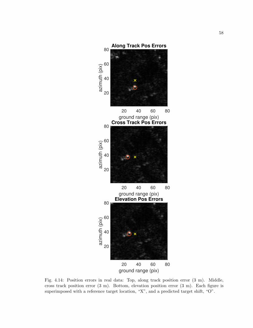
58

Along Track Pos Errors

20 40 60 80

ground range (pix)

20

40

60

80

azim

uth

(p

ix)

Cross Track Pos Errors

20 40 60 80

ground range (pix)

20

40

60

80

azim

uth

(p

ix)

Elevation Pos Errors

20 40 60 80

ground range (pix)

20

40

60

80

azim

uth

(p

ix)

Fig. 4.14: Position errors in real data: Top, along track position error (3 m). Middle,cross track position error (3 m). Bottom, elevation position error (3 m). Each figure issuperimposed with a reference target location, “X”, and a predicted target shift, “O”.

59

Along Track Vel Errors

20 40 60 80

ground range (pix)

20

40

60

80

azim

uth

(p

ix)

Cross Track Vel Errors

20 40 60 80

ground range (pix)

20

40

60

80

azim

uth

(p

ix)

Elevation Vel Errors

20 40 60 80

ground range (pix)

20

40

60

80

azim

uth

(p

ix)

Fig. 4.15: Velocity errors in real data: Top, along track velocity error (1 m/s). Middle,cross track velocity error (0.2 m/s). Bottom, elevation velocity error (0.2 m/s). Each figureis superimposed with a reference target location, “X”, and a predicted target shift, “O”.

60

Roll Errors

20 40 60 80

ground range (pix)

20

40

60

80

azim

uth

(p

ix)

Pitch Errors

20 40 60 80

ground range (pix)

20

40

60

80

azim

uth

(p

ix)

Yaw Errors

20 40 60 80

ground range (pix)

20

40

60

80

azim

uth

(p

ix)

Fig. 4.16: Attitude errors in real data: Top, roll error (0.01 rad). Middle, pitch error (0.5rad). Bottom, yaw error (0.1 rad). Each figure is superimposed with a reference targetlocation, “X”, and a predicted target shift, “O”.

61

CHAPTER 5

GPS-DENIED NAVIGATION USING SYNTHETIC APERTURE RADAR AND

KNOWN TARGET LOCATIONS

Past research has explored the feasibility of using radar telemetry in conjunction with

an inertial navigation system to perform GPS denied navigation. The research presented

in this paper further explores GPS denied navigation using radar by extracting range and

cross range measurements from synthetic aperture radar images formed using the range

Doppler algorithm. An inertial navigation and radar processing system is implemented

using both real and simulated radar images to aid in estimating an aircraft’s state in a GPS

denied environment. Results and discussion have been provided. The results show that

navigating in the absence of GPS using synthetic aperture radar is feasible with converging

and bounded estimation errors.

5.1 Introduction

GPS denied navigation is the study of precisely navigating a vehicle in the absence of

a Global Navigation Satellite System (GNSS) such as GPS. This can be accomplished in

a variety of ways and is a very active field of research. Current research is exploring the

feasibility of using synthetic aperture radar (SAR) as a means of navigating without GPS.

SAR is a method of processing radar data to form images of a landscape, typically from an

aircraft or spacecraft. The research presented in this paper expands on previous research

and further tests the feasibility of using radar telemetry to aid in GPS denied navigation.

Specifically, the research presented here explores methods of extracting navigation in-

formation from fully formed SAR images. Images are created using the range Doppler

algorithm (RDA), which is an efficient Fourier based image formation technique. Navi-

gation measurements are extracted from images through a comparison with known target

location data. Measurements are applied to a local coordinate frame and take the form of

62

range and cross range measurements.

A full flight simulation and radar simulation are implemented and verified via a Monte

Carlo analysis. Algorithms developed in the simulated system are applied to navigation

and radar data collected in Logan, Utah by the Space Dynamics Laboratory. Results from

both the simulated system and real system are provided.

5.1.1 Literature Review

This research is conceptually organized into three categories: GPS denied navigation,

SAR image formation, and measurement extraction from SAR images.

GPS denied navigation

GPS is integral in most navigation systems. Without GPS, a navigation system loses

knowledge of position, velocity, and attitude, and estimates of the vehicle state experience

error. Situations of GPS denial occur in a variety of situations. For example, GPS is easily

jammed or spoofed. GPS can also be denied by natural or manmade structures obscuring

the sky. Without GPS, a vehicle must rely on other forms of information to precisely

navigate.

GPS denied navigation is typically performed using accelerometers and gyroscopes cou-

pled with a selection of auxiliary sensors, from which auxiliary measurements are collected.

Examples of possible auxiliary sensors include lidar, cameras, radar, range finders, etc, [16].

The auxiliary sensors attempt to supply knowledge sufficient to replace the knowledge lost

by GPS.

Radar is one of the auxiliary sensors currently being researched for this purpose. Some

advantages of radar are that its pulses can penetrate cloud cover and are actively illumi-

nating. As such, images of a landscape using SAR can be formed during stormy weather

and at night. This presents an advantage over other imaging systems that employ cameras,

which can’t image at night or during inclement weather, or lidar which may have trouble

in inclement depending on illumination wavelengths.

63

Many methods for using radar as a supplementary sensor have been explored. These

methods of navigation can be generally classified into two categories: relative navigation

and absolute navigation. Absolute navigation places the vehicle on a global coordinate

system such as latitude, longitude, and altitude. Relative navigation places the vehicle on

a local coordinate system originating from some known feature or location.

In recent radar aided navigation literature, absolute and relative navigation can be split

into several subcategories. Absolute radar aided navigation can be split into methods using

terrain matching and methods using SAR images. Relative radar aided navigation can be

split into methods using generic radar odometry, methods using Simultaneous Localization

and Mapping, and methods again using SAR images. Each of these subcategories is briefly

presented here.

Terrain contour matching is one approach to absolute radar aided navigation. Terrain

contour matching is a scheme that exploits variations in terrain height along the flight

path of an aircraft to determine the location of the vehicle in a global reference frame.

Variations in terrain can be measured from radar nadir bounces or from interferometric

SAR. These methods have been explored by Hollowell et al, Bergmann et al, Nordlund and

Gustafsson, and more, each approach varying in complexity, from grids of Kalman filters to

marginalized particle filters [28–32]. Of note is work done by Kim et al [33] measurements

from an interferometric radar altimeter (IRA) provide the range to the nearest point to the

radar vehicle from the underlying terrain. This measurement is processed together with

information from a Digital Elevation Model (DEM) in a particle filter to predict a unique

trajectory. Simulation results show ¡3 meters rms of absolute estimation error. The major

factor in navigation accuracy is the accuracy of the DEM.

Absolute radar aided navigation using SAR images has been explored by the SARINA

project [6,7,34–37]. The SARINA project uses prominent features in SAR images correlated

to features within a reference map. In the case of mountainous regions, a DTED is used to

synthesize an Interferometric SAR (InSAR) image, which is then compared to the InSAR

image produced from the radar data. Divak approached the radar-aided absolute navigation

64

problem by simulating reference SAR images using 3D terrain data and electro-optical

imagery, then comparing it to a real SAR image over the same area [38].

Relative radar aided navigation has been explored using general radar odometry. Scan-

napieco et al. detected ground targets using a constant false alarm rate and tracked their

position using global nearest neighbor in range compressed data [39, 40]. Beard et al. ex-

ploited the fact that for linear flight paths, prominent reflectors manifest themselves as

hyperbolic curves in the range-compressed vs. time image, [9, 11]. Features were tracked

using a hyperbolic Hough transform, after which successive pairs of range measurements

were used to determine changes in horizontal position. Altitude above ground level was de-

termined from the nadir radar return. Mostafa et al, developed a combined radar odometry

and visual odometry method and demonstrated performance on real data [41].

Simultaneous Localization and Mapping (SLAM) is another example of relative navi-

gation. Where odometry approaches contains only states of the vehicle, SLAM approaches

augment the vehicle states with the position of the reflectors in an EKF framework. The

SLAM approach was studied over a period of five years by a group from the Air Force

Institute of Technology [13, 42–48]. They developed a SLAM architecture that utilized the

range-compressed radar data to detect, track, then estimate both the vehicle and reflector

states culminating in a hardware implementation with highly reflective targets. Quist et

al. extended research relying on the Hough transform by implementing a more efficient

Recursive-RANSAC algorithm for data association and tracking of reflectors [12]. Here,

reflector states were included in the state vector, resulting in a SLAM framework, which

was demonstrated on real outdoor flight data.

Relative navigation using SAR images is less explored, but typically involves using an

autofocusing algorithm to estimate velocity errors. Samczynski provides a discussion on the

different approaches in this field [49,50].

The research in this paper performs absolute navigation using SAR images coupled

with known target position information along the flight trajectory. The targets are chosen

such that they follow the trajectory of the vehicle in a “breadcrumb” like fashion. This

65

allows for known targets to be visible to the radar antenna at most points in the trajectory.

This arrangement is representative of SAR images collected near towns, diverse landscapes,

wooded areas, roads, etc.

Synthetic Aperture Radar

Synthetic aperture radar (SAR) is an imaging technique based on the transmission

of radar pulses at intervals along the trajectory of some vehicle. The transmitted energy

bounces off ground targets and returns to the radar receiver. After collecting data along a

sufficiently long section of the trajectory, the received radar pulses are processed into images.

Radar pulses can penetrate cloud cover and is actively illuminating. As such, images of a

landscape using SAR can be formed during stormy weather and at night. This presents an

advantage over other imaging techniques such as optical cameras or lidar systems.

Forming SAR images is a process of matched filtering. Several algorithms exist to

process SAR data into images. Differences in image formation algorithms boil down to

differences in how matched filtering is performed. For stripmap mode SAR, images can

be formed using the back-projection algorithm (BPA) where images are processed with a

time domain matched filter on hyperbolic curves in the data. The time domain matched

filter is flexible in that it can accommodate complicated flight trajectories, but it is com-

putationally expensive and sensitive to navigation errors. As such, the BPA requires high

precision navigation data to form accurate images. Images can also be formed using RDA,

which performs matched filtering in the frequency domain after range cell migration cor-

rection. The frequency domain filter is computationally less expensive and less sensitive

to navigation errors than a time domain filter, but typically requires a straight trajectory

to form accurate images. Other image formation algorithms for stripmap SAR include the

Omega-K algorithm and the chirp scaling algorithm [3].

The research in this paper will use RDA to form images and SAR based measurements.

RDA images are less sensitive to navigation error than BPA images. As such RDA can form

measurable images in environments with errors that would leave BPA images unmeasurable.

Additionally, this research is aimed toward navigation of light aircraft such as UAVs. The

66

computationally less expensive option is attractive for the potentially smaller processing

packages available to UAVs. Because RDA forms images for straight trajectories, a straight

flight assumption will be made in later sections to extract measurements from the RDA

SAR images.

SAR imagers are dependent on vehicle position and velocity. Because of this depen-

dence, errors trajectory estimation will result in errors in the final SAR image. Of particular

note is that position estimation errors cause target shifting in the image, and velocity es-

timation errors cause target shifting and blurring [2]. Research performed at Utah State

University hypothesizes that GPS denied navigation can be performed based on the SAR

image error characteristics [17]. The research in this paper expands on that idea and uses

corrupted images as a source of measurements in the navigation algorithm.

Measurement Extraction

This research is, in part, an extension of research done by Lindstrom et al, where

the feasibility of GPS denied navigation was explored using range and range-rate measure-

ments from radar telemetry [1]. In their research, range and range-rate measurements were

synthesized from the estimated trajectory of an aircraft rather from radar data.

Here, a slightly different system will be implemented that extracts range and cross range

position measurements from SAR images. Cross range measurements can be obtained si-

multaneously with range measurements, which provides an opportunistic advantage over

range-rate measurements. The combination of range and cross range measurements is sim-

ilar to the proposed system described by Nitti et al in their feasibility study [6].

Radar data can be collected and processed to various types of information, each with

its own computational complexity. These types include raw radar return data (a.k.a. phase

history), range compressed data, and fully formed images. Each type of data has different

uses in navigation. For example, range measurements can be obtained from fully formed

SAR images by calculating the distance between a location in the image to the radar vehicle.

This calculation is straightforward when the SAR algorithm forms images in the slant range

dimension, as is the case with RDA. Images formed in the ground range dimension require

67

an estimate of vehicle altitude above the ground, which may not be accurate or available

in the absence of GPS and a DEM.

To form accurate cross range measurements, the time of closest approach (TOC) to any

particular target must be known. The TOC is the moment in time when the radar vehicle

is closest to the target in question. It is related to the Doppler of the azimuth signal,

which requires accurate Doppler parameter estimation. Cumming et al and Li et al have

shown methods to properly estimate Doppler parameters such as the Doppler centroid and

Azimuth FM rate [51], [52], [3]. Examples of these methods include clutterlock and image

autofocusing techniques. Wei et al combines least square regularization and minimum mean

square error techniques to autofocus a SAR image from which model parameters can be

estimated [53]. In this research, multilook misregistration autofocusing is used to estimate

the Doppler parameters of the system.

Section 5.2 provides a background on SAR image formation using RDA. Section 5.3

develops a navigation system conducive to Monte Carlo analysis using SAR image measure-

ments incorporated via an EKF. Section 5.4 summarizes results of the research and provides

discussion. Section 5.5 concludes the document and suggests areas of future work. An ap-

pendix is included to provide additional details on multilook misregistration autofocusing,

which is a processing step employed in section 5.3.

5.2 Background

This section is a self-contained tutorial on the range-Doppler Algorithm, as its use may

be unfamiliar to those in the field of GPS-denied navigation. RDA is a SAR image formation

technique that takes advantage of the Fourier domain to perform efficient matched filtering.

The basic RDA algorithm can be summarized into the following steps:

1. Collect raw radar data

2. Perform range compression

3. Compute FFT in the azimuth dimension

4. Compensate for range cell migration

5. Perform azimuth compression

68

6. Return data to spatial domain

The process of forming RDA images begins by transmitting radar pulses at multiple

points along a vehicle trajectory. These pulses reflect off ground targets and are collected

by the radar receiver as raw SAR data. Radar pulses can have various structures but are

usually of a linear frequency modulated (LFM) form. LMF signals, or “chirp” signals, are

characterized by an instantaneous frequency that varies linearly with time. The transmitted

LFM signal stx(t) is written as

stx(t) =

exp(j2πf0t+ jπKt2), 0 ≤ t ≤ T

0, otherwise

(5.1)

where f0 is the initial frequency, K is the linear FM rate in Hz/s, and T is the pulse

duration.

The return LFM signal is denoted srx(t). The return signal is written using a “stop

and hop” assumption, which assumes the vehicle transmits and receives each radar pulse

without traversing any distance.

srx(t) = Astx(t− τ) (5.2)

In this equation, A is the attenuation of the signal and τ is the time delay between the

transmitted and received signal.

After collecting raw radar data, the data is fed through a matched filter in the range

dimension to perform “range compression”. The matched filter is a time reversed, conjugate

version of the transmitted signal stx(t), which is denoted g(t). For efficiency, the matched

filter is applied in the frequency domain. Let a capital letter denote a signal in the frequency

69

domain. The result of matched filtering is denoted sout(t), and is equal to

sout(t) = srx(t) ∗ g(t) (5.3)

= F−1 {F {srx(t)} ·F {g(t)}}

= F−1 {Srx(f) ·G(f)}

Each output of the matched filter is collected together to form the aggregate range

compressed data, which will be denoted src(t, η). Note that the range compressed data is

not just a function of range time t, but also azimuth time η. Visually, range compressed

data appears as a composition of several hyperbolic arcs overlaid on top of each other. Each

hyperbolic arc represents a ground target. This is illustrated in Figure 5.1.

Azimuth compression begins by taking an FFT of the range compressed data in the

azimuth dimension. The data in the range dimension is left in the time domain. The

azimuth-frequency range-time domain is referred to as the range-Doppler domain. The

data in the range-Doppler domain is denoted,

Fη {src(t, η)} = Src(t, fη) (5.4)

Note that the η subscript on F denotes the FFT in the azimuth dimension. Range cell

migration correction must be applied before applying a matched filter to range-Doppler

data. Range cell migration refers to the hyperbolic shape of the targets in the data. Each of

these hyperbolic arcs must be reformatted to form a straight line within the data. Without

correcting for range cell migration, the final image will blur, and resolution will decrease.

Figure 5.2 shows the data in the range Doppler domain before and after range cell migration

correction

Range cell migration correction can be performed by re-indexing each row of the range-

Doppler data according to a correction factor. The amount of correction required for each

70

0 100 200 300

East(m)

-50

0

50

100

150

Nort

h(m

)

Trajectory and Ground Targets

Flight Trajectory

Start

Finish

Reflectors

Range Compressed Data

1325 1330 1335 1340 1345

Range (m)

0

20

40

60

80

100

Azim

uth

(m

)Fig. 5.1: Illustration of how ground targets at various locations (Left) become hyperboliccurves in the range compressed data (Right).

Before Range Cell Migration Correction

Range (m)

Dopple

r (H

z)

After Range Cell Migration Correction

Range (m)

Dopple

r (H

z)

Fig. 5.2: Illustration of the data in the range Doppler domain before (Left) and after (Right)range cell migration correction.

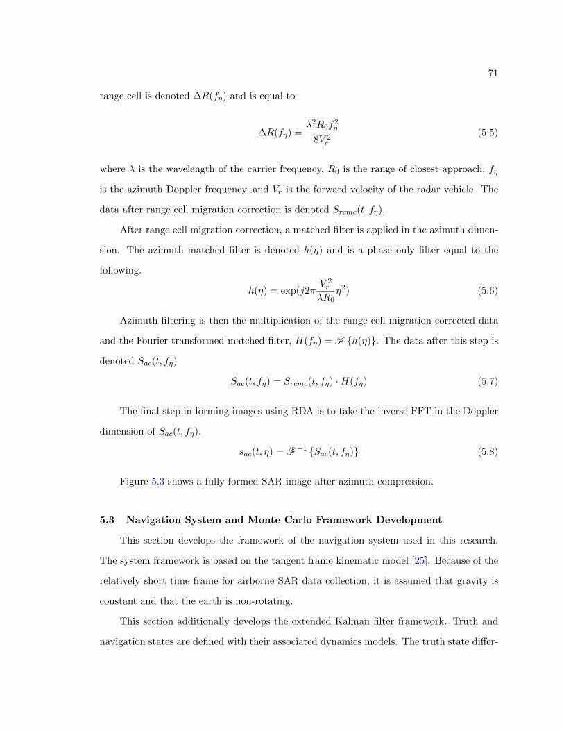
71

range cell is denoted ∆R(fη) and is equal to

∆R(fη) =λ2R0f

2η

8V 2r

(5.5)

where λ is the wavelength of the carrier frequency, R0 is the range of closest approach, fη

is the azimuth Doppler frequency, and Vr is the forward velocity of the radar vehicle. The

data after range cell migration correction is denoted Srcmc(t, fη).

After range cell migration correction, a matched filter is applied in the azimuth dimen-

sion. The azimuth matched filter is denoted h(η) and is a phase only filter equal to the

following.

h(η) = exp(j2πV 2r

λR0η2) (5.6)

Azimuth filtering is then the multiplication of the range cell migration corrected data

and the Fourier transformed matched filter, H(fη) = F {h(η)}. The data after this step is

denoted Sac(t, fη)

Sac(t, fη) = Srcmc(t, fη) ·H(fη) (5.7)

The final step in forming images using RDA is to take the inverse FFT in the Doppler

dimension of Sac(t, fη).

sac(t, η) = F−1 {Sac(t, fη)} (5.8)

Figure 5.3 shows a fully formed SAR image after azimuth compression.

5.3 Navigation System and Monte Carlo Framework Development

This section develops the framework of the navigation system used in this research.

The system framework is based on the tangent frame kinematic model [25]. Because of the

relatively short time frame for airborne SAR data collection, it is assumed that gravity is

constant and that the earth is non-rotating.

This section additionally develops the extended Kalman filter framework. Truth and

navigation states are defined with their associated dynamics models. The truth state differ-

72

Range Doppler Image (Slant Range)

1320 1330 1340 1350

Range (m)

40

45

50

55

60

Cro

ss R

ange (

m)

Fig. 5.3: Fully formed SAR image after azimuth matched filtering and inverse FFT.

ential equations are linearized about the navigation state to derive the linear dynamics of

the estimation errors used within the EKF. The three states used in developing the EKF,

the truth state, the navigation/estimated state, and error state, will be defined in relation

to the “north, east, down” or n coordinate system. Measurement models using SAR images

are developed. Finally, the Kalman filter equations are presented.

5.3.1 Truth and Navigation Models

The truth state is defined as the actual state of the vehicle as though it were measured

with completely noiseless, zero bias instruments. The truth state is denoted x and behaves

73

according to the truth dynamics (or truth model), denoted x.

x =

pn

vn

qnb

ba

bg

bh

br

bc

, x =

vn

Tnb νb + gn

qnb ⊗12

[0ωb

]− 1τa

ba + wa

− 1τg

bg + wg

− 1τhbh + wh

− 1τrbr + wr

− 1τcbc + wc

(5.9)

In this definition, pn is the position vector, vn is the velocity vector, qnb is the attitude

quaternion which transforms from the body frame, b, to the n frame, and each bi term is a

sensor bias term governed by a first order Markov model. For each bias term, 1τi

is the time

constant and wi is process noise. The bias terms are for the accelerometer (a), gyroscope

(g), altimeter (h), radar range measurements (r), and radar cross range measurements (c).

Note νb and ωb are measurements from the accelerometer and gyroscope, respectively.

gn is used to represent the gravitational constant. The ⊗ symbol is used to denote quater-

nion multiplication. Lastly, Rnb is a rotation matrix that rotates the accelerometer mea-

surement into the n frame from the b frame.

The estimated state is defined as the state of the vehicle according to current estimates

resulting from instruments and Kalman filtering. It is expected that noise will be present

in the estimated state. The estimated state is denoted x and behaves according to the

navigation model (or navigation dynamics), which are denoted ˙x. Note that the estimated

state and navigation model are nearly identical to the truth state and truth model. In the

navigation model, bias terms are not propagated with process noise, as it is unknown to

the filter. Additionally, each accelerometer and gyroscope measurement is compensated for

74

by the current bias estimate as opposed to the true bias.

x =

pn

vn

qnb

ba

bg

bh

br

bc

, ˙x =

vn

Tnb

(νb − ba) + gn

qnb ⊗12

[0

ωb−bg

]− 1τa

ba

− 1τg

bg

− 1τhbh

− 1τrbr

− 1τcbc

(5.10)

The true values of specific force and angular rate are related to the measurement values,

sensor biases, and noise,

νb = νb + ba + nν (5.11)

ωb = ωb + bg + nω (5.12)

where nν and nω are sensor noise vectors.

5.3.2 Linear Error Model

The error state is defined as the perturbation between the truth state and estimated

state. This perturbation is given by

δpn = pn − pn (5.13)

δvn = vn − vn (5.14) 1

−12δθ

n

= qnb ⊗ (qnb )∗ (5.15)

δbi = bi − bi (5.16)

75

where a δ denotes an element of the error state. The subscript i on δbi is an index indicating

any of the various bias terms.

The error state is governed by a linear model formed by linearizing the truth model

about the estimated state. The result of the linearization is a model of the form

δx = F δx +Bw (5.17)

where F is,

F =

F11 F12

09×9 F22

(5.18)

F11 =

0 I 0

0 0 [Rnb(νb − ba)]×

0 0 0

(5.19)

F21 =

0 0 0 0 0

−Rnb

0 0 0 0

0 Rnb

0 0 0

(5.20)

F22

− 1τaI 0 0 0 0

0 − 1τgI 0 0 0

0 0 − 1τh

0 0

0 0 0 − 1τr

0

0 0 0 0 − 1τc

(5.21)

The matrix B is a noise coupling matrix and is given by,

B =

B11 09×9

09×9 I9×9

(5.22)

76

B11 =

0 0

−Rnb

0

0 Rnb

(5.23)

The vector w is the noise vector and comprises accelerometer and gyroscope measurement

noise as well as the process noise driving the sensor bias states.

w = [nν ,nω,wa,wg, wh, wr, wc]T (5.24)

Note the “cross” operator, ×, which is defined as,

× : R3 → R3×3, s.t. ∀a ∈ R3, (a×) =

[0 −a3 a2a3 0 −a1−a2 a1 0

]

5.3.3 Measurement Model

The measurement model is comprised of three different measurements. These are the

range, cross range, and altitude measurements. All measurements are taken at the time of

closest approach for the target corresponding to the given measurement. This means the

range and cross range measurements will reveal offsets from the estimated range of closest

approach and time of closest approach, respectively. Altitude measurements are taken to

resolve an ambiguity that arises in range measurements between cross track and elevation

errors.

The range and cross range measurements assume knowledge of a target location. For

the purposes of this research, it is assumed that knowledge of the target location comes

in the form of a previously-collected SAR image. Other formats of target knowledge are

possible and can be implemented for specific system needs. Offsets from true target locations

are found using a two-dimensional cross correlation between the collected SAR image and a

reference SAR image, both of which are formed in the slant range dimension. The location

of the peak of the cross correlation is used to find the offset from the true target location.

The offsets are used to calculate the range and cross range measurements. This process is

illustrated in Figure 5.4.

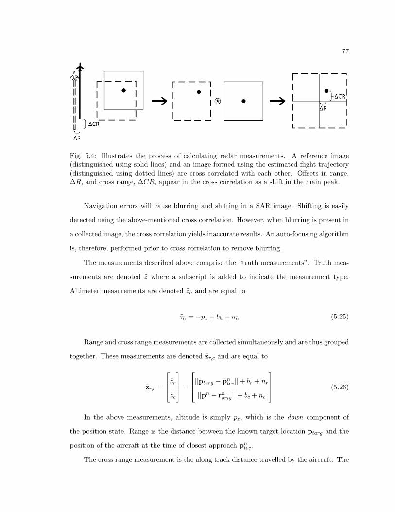
77

Fig. 5.4: Illustrates the process of calculating radar measurements. A reference image(distinguished using solid lines) and an image formed using the estimated flight trajectory(distinguished using dotted lines) are cross correlated with each other. Offsets in range,∆R, and cross range, ∆CR, appear in the cross correlation as a shift in the main peak.

Navigation errors will cause blurring and shifting in a SAR image. Shifting is easily

detected using the above-mentioned cross correlation. However, when blurring is present in

a collected image, the cross correlation yields inaccurate results. An auto-focusing algorithm

is, therefore, performed prior to cross correlation to remove blurring.

The measurements described above comprise the “truth measurements”. Truth mea-

surements are denoted z where a subscript is added to indicate the measurement type.

Altimeter measurements are denoted zh and are equal to

zh = −pz + bh + nh (5.25)

Range and cross range measurements are collected simultaneously and are thus grouped

together. These measurements are denoted zr,c and are equal to

zr,c =

zrzc

=

||ptarg − pntoc||+ br + nr

||pn − rnorig||+ bc + nc

(5.26)

In the above measurements, altitude is simply pz, which is the down component of

the position state. Range is the distance between the known target location ptarg and the

position of the aircraft at the time of closest approach pntoc.

The cross range measurement is the along track distance travelled by the aircraft. The

78

along track distance can be measured on either a global coordinate system with the origin

being the beginning of the flight trajectory, or on a local coordinate system with the origin

being arbitrarily chosen. The origin point is denoted rnorig and is chosen to be located within

the subaperture. This measurement formulation assumes straight flight. As this assumption

is more likely to be true during radar data collection, the model in this paper assumes a

local coordinate system centered on an origin located within the trajectory of the current

SAR image’s subaperture.

Each measurement defined above can be taken at any point within a SAR image’s

subaperture. During implementation, it is chosen to collect and process measurements

at the time of closest approach to the target within the current image. Note that, each

measurement in the model is corrupted by both bias, bi, and noise, ni.

Analogous to the truth measurements z, are the estimated measurements, which are

denoted ˆz. The equations describing the behavior of estimated measurements are nearly

identical to the true measurement equations but lacks any knowledge of noise terms and

uses estimated states to calculate each measurement.

ˆzh = −pz + bh (5.27)

ˆzr,c =

ˆzr

ˆzc

=

||ptarg − pntoc||+ br

||pn − rnorig||+ bc

(5.28)

The difference between the true measurements z and estimated measurements ˆz is

called the “residual” and is used in the EKF to update the estimate of the error state.

The linearization of the truth model around the navigation state is given as,

δz = Hδx + γ (5.29)

79

where H is the sensitivity matrix for the measurements. H is found by taking the Jacobian

of each truth measurement and evaluating about the estimated state. This results in

H =

H1

H2

(5.30)

where H1 is the sensitivity matrix for the altimeter measurement and is equal to

H1 =

[[0, 0,−1] 01×12

](5.31)

H2 is the sensitivity matrix for the radar range and cross range measurements and is

equal to

H2 =

−dT||d|| 01×12

−lT||l|| 01×12

(5.32)

where d = ptarg − pntoc and l = pn − rnorig. The vector γ is measurement noise and is equal

to

γ = [nr, nc, nh]T (5.33)

5.3.4 Covariance Propagation

With states, models, and measurements defined and the appropriate linearizations

performed, the structure of the EKF can be built. This begins with initialization and

propagation of the covariance matrix. The covariance of the error state is initialized using

a steady state covariance matrix from an INS processing GPS measurements. This mimics

the situation when GPS is denied mid-flight. The covariance of the error state is then

propagated forward in time as

P = FP + PF +BQBT (5.34)

where F and B are defined previously.

80

The Q matrix is the power spectral density of the noise vector w. Assuming the noise

is zero mean, gaussian, and independent, Q is a diagonal.

Q = diag(σ2vrwI3×3, σ

2arwI3×3,

2σ2ss,ba

τaI3×3, (5.35)

2σ2ss,bg

τgI3×3,

2σ2ss,bh

τh,2σ2

ss,br

τr,2σ2

ss,bc

τc)

When a measurement becomes available from the radar imaging system, a Kalman

update is performed. To perform a Kalman update, the Kalman gain is first calculated,

which is given by

K = P−HT [HP−HT +GRGT ]−1 (5.36)

where P− is the error state covariance before the Kalman update, and R is the covariance of

the noise on the available measurement. The matrix H varies between H1 and H2 depending

on the type of measurement available.

The Kalman gain is then used to update the error state covariance using the Joseph

form,

P+ = [I −KH]P−[I −KH]T +KGRGTKT (5.37)

The Kalman gain and measurement residual is also used to update the estimate of the

error state.

δx+ = K[z− ˆz] (5.38)

After updating the estimate of the error state vector, the new error is applied to the

navigation state, which forms an updated navigation state vector. This update is performed

as,

81

x+ =

(pn)− + δpn

(vn)− + δvn[1

− 12δθnb

]⊗ (qn

b)−

(ba)− + δba

(bg)− + δbg

(bh)− + δbh

(br)− + δbr

(bc)− + δbc

(5.39)

5.4 Results

The system described above is implemented on both simulated and real data. Results

of both types of data are given in this section. Loosely coupled GPS measurements are used

to calibrate initial bias estimates and initial covariance matrices. After calibration, GPS

measurements cease, and the aircraft begins navigating using SAR images.

5.4.1 Simulated Data

A full flight and radar processing simulation was created to test the feasibility of the

work described in the previous sections. The true flight trajectory is a straight and level

flight flying northward. Initial errors are injected into the true trajectory and are propagated

forward to create the estimated trajectory. The radar scene is a random field of radar

scatterers dense enough to ensure that a few targets appear in every SAR image. The flight

is fifty seconds long and is split into fifty subapertures, each one being one second long.

In the simulation, an aircraft flies along the true trajectory and collects radar data. At

the end of each subaperture, a SAR image is formed using RDA and the estimated vehicle

state. Measurements are extracted and applied in the EKF using the method described in

Section 5.3.3. The true trajectory and the estimated trajectory produced by the EKF are

compared, and estimation errors are calculated.

In the simulation, accelerometer and gyroscope measurements are synthesized with

82

added zero mean gaussian noise. Noise is consistent with a tactical grade inertial measure-

ment unit (IMU). Tactical grade measurements are chosen to mimic the quality of the data

used in the real data implementation.

Noise is also added to the radar measurements to better mimic measurements from the

real data. Because the radar measurements rely on a cross correlation to infer distances,

the quality of the measurement depends heavily on the quality of the reference target

information and the radar scene being imaged. Radar scenes with very diffuse or very

sparse targets may produce an inaccurate cross correlation, leading to an inaccurate range

or cross range measurement.

Tables 5.1 and 5.2 summarizes the parameters used for both the navigation system and

radar system.

Table 5.1: Summary of radar parameters used in simulation.

SAR Parameter Value

RF center frequency 9.75 GHzBandwidth 500 MHz

Range over-sample rate 2Range resolution 0.15 m

PRF 100 HzInitial Velocity 10 m/secAntenna squint 0.0 deg

Ideal azimuth resolution 0.1 mRange offset 2000 m

Min/Max range 2000 m/2210 mSub aperture length 1 sec (10 m)

Table 5.2: Summary of navigation parameters used in simulation.

Navigation Parameter Value

Velocity random walk 0.1 m/s/sqrt(hr)Initial Accelerometer bias 0.01 g

Angular random walk 0.1 deg/sqrt(hr)Initial Gyroscope bias 5 deg/hr

Altimeter standard deviation 1.3 mRange standard deviation 0.25 m

Cross range standard deviation 0.25 m

83

The results of the simulated Monte Carlo analysis are provided in Figures 5.5 through

5.8. Each of the figures shows a collection of solid lines mostly bounded by a set of dashed

lines. Each solid line represents a single run of the Monte Carlo simulation. Each dotted

line represents a 3-sigma bound inside which the solid lines should mostly fall.

Figure 5.5 shows only one set of solid lines each. This figure plots the residual mea-

surement z − ˆz for one of the Monte Carlo runs. According to Kalman filter theory, the

residuals should be white and zero mean in structure. This figure provides a visual confir-

mation of the residuals meeting these requirements. Figure 5.6 shows the estimation error

in the position states, calculated as the difference between the true and estimated trajec-

tories. Figures 5.7 and 5.8 show similar information for the aircraft velocity and attitude,

respectively.

The results show that the proposed navigation and radar system are capable of esti-

mating the aircraft state in the absence of GPS. The measurement residuals are white and

zero mean. The estimation error converges and remains bounded over the course of the

full trajectory. The position is estimated in all dimensions to within 3 meters. Velocity is

estimated to within 0.5 meters per second. North and east attitudes are estimated within

2 milli-radians, and down attitude is estimated withing 7 milli-radians.

5.4.2 Real Data

A system similar to that for the simulated data was implemented to process real flight

and radar data. As with simulated data, the real flight length is fifty seconds, which is split

into fifty sub-apertures, each sub-aperture being one second long.

Flight and radar data were collected and provided by the Space Dynamics Lab (SDL)

in Logan, Utah. The data were collected on their FlexSAR system, a low-cost, high quality

prototyping SAR instrument [54], paired with a NovAtel SPAN CPT7 tactical grade IMU

[55]. A GPS based navigation solution is available for the trajectory, which is taken to be

the “truth” trajectory. This solution is achieved via post-processing in Waypoint software

by NovAtel and is accurate to about 1 cm. Altimeter measurements were synthesized using

parameters based on the Honeywell Precision Barometer HPB [56].

84

0 10 20 30 40 50

time(s)

-5

0

5

Altim

ete

r R

esid

ual(m

) Residual

Residual cov

0 10 20 30 40 50

time(s)

-4

-2

0

2

4

Range R

esid

ual(m

)

Residual

Residual cov

0 10 20 30 40 50

time(s)

-3

-2

-1

0

1

2

3

Cro

ss R

ange R

esid

ual(m

)

Residual

Residual cov

Fig. 5.5: Measurement residuals for altimeter measurements (Top), range measurements(Middle), and cross range measurements (Bottom). Dotted lines signify 3 sigma bounds,and solid lines represent residual measurements.

85

Fig. 5.6: Estimation errors for north position (Top), east position (Middle), and downposition (Bottom). Dotted lines signify 3 sigma bounds. Individual solid lines representindividual runs of the Monte Carlo simulation.

86

Fig. 5.7: Estimation errors for north velocity (Top), east velocity (Middle), and downvelocity (Bottom). Dotted lines signify 3 sigma bounds. Individual solid lines representindividual runs of the Monte Carlo simulation.

87

Fig. 5.8: Estimation errors for north attitude (Top), east attitude (Middle), and downattitude (Bottom). Dotted lines signify 3 sigma bounds. Individual solid lines representindividual runs of the Monte Carlo simulation.

88

Tables 5.3 and 5.4 list parameters specific to the instruments used in data collection.

Table 5.3: Summary of radar parameters from the FlexSAR system.

SAR Parameter Value

RF center frequency 9.75 GHzBandwidth 500 MHz

Range over-sample rate 1Range resolution 0.2998 m

PRF 5000 Hz (decimated to 1667 Hz)Initial Velocity 60 m/secAntenna squint 0.0 deg

Ideal azimuth resolution 0.0378 mRange offset 1948 m

Min/Max range 1948 m/2112 mSub aperture length 1 sec ( 60 m)

Table 5.4: Summary of navigation parameters from the FlexSAR system.

Navigation Parameter Value

Velocity random walk 0.1 m/s/sqrt(hr)Initial Accelerometer bias 0.0033 g

Angular random walk 0.1 deg/sqrt(hr)Initial Gyroscope bias 4.0758 deg/hr

Altimeter accuracy (3σ) 0.4 hPa

For real data, a single iteration of flight estimation is performed. Accelerometer and

gyroscope measurements are provided in the data set and are used to propagate the navi-

gation state forward in time. At the end of each subaperture, a SAR image is formed, and

measurements are extracted and applied to the estimated state via the EKF. estimation

errors are recorded throughout the flight and are displayed. At the end of the flight, state

estimation errors are calculated and displayed.

Estimation results are shown in Figures 5.9 through 5.12. These again illustrate the

performance of the system in terms of residuals and estimation errors. Figure 5.9 provides

a visual confirmation that the measurement residuals are zero mean and white.

Over the course of a fifty second GPS denied flight, the estimation errors remain

89

0 20 40 60

time(s)

-6

-4

-2

0

2

4

6

Altim

ete

r R

esid

ual(m

) Residual

Residual cov

0 20 40 60

time(s)

-4

-2

0

2

4

Range R

esid

ual(m

)

Residual

Residual cov

0 20 40 60

time(s)

-3

-2

-1

0

1

2

3

Cro

ss R

ange R

esid

ual(m

)

Residual

Residual cov

Fig. 5.9: Measurement residuals from the real data set for the altimeter measurements(Top), range measurements (Middle), and cross range measurements (Bottom). Dottedlines signify 3 sigma bounds, and solid lines represent residual measurements.

90

Fig. 5.10: Estimation errors from the real data set for north position (Top), east position(Middle), and down position (Bottom). Dotted lines signify 3 sigma bounds. Solid linesrepresent actual estimation error.

91

Fig. 5.11: Estimation errors from the real data set for north velocity (Top), east velocity(Middle), and down velocity (Bottom). Dotted lines signify 3 sigma bounds. Solid linesrepresent actual estimation error.

92

Fig. 5.12: Estimation errors from the real data set for north attitude (Top), east attitude(Middle), and down attitude (Bottom). Dotted lines signify 3 sigma bounds. Solid linesrepresent actual estimation error.

93

bounded within the 3-sigma covariance lines. Position errors stay bounded within ap-

proximately 3 meters. Velocity errors stay bounded within approximately 0.4 meters per

second. Attitude errors stay bounded within approximately 7 milli-radians in the north

and east case and 15 milli-radians in the down case. These results are very similar to the

simulated data case, which uses similar parameter and initialization values to best mimic

the real data case.

To highlight the effect of the radar measurements on estimation errors, Figure 5.13

has been provided. This figure plots estimation errors bounds for north, east and down

positions. Each sub-figure shows two bounds on a logarithmic scale. The dotted line

represents the estimation error 3σ bound when no SAR measurements are processed. The

solid line shows the same bound when SAR measurements are processed. Notice that

omission of SAR measurements degrades the north and east estimates, and they begin to

grow without bound. The down estimate stays bounded due to altimeter measurements.

5.5 Conclusion

This paper furthers the research done in absolute radar aided GPS denied navigation

using RDA SAR images. The feasibility of extracting navigation information from RDA

SAR images is demonstrated. Range and cross range measurements were extracted from

RDA SAR images via comparing to known target locations and processed in an indirect

extended Kalman filter. Both simulated data and real data were analyzed. Estimation using

simulated data was shown to have converging estimation errors and be bounded within 3-

sigma values of the state covariance matrix. Estimation errors using the real data were

similarly bounded. In both cases, errors in position were estimated with approximately 3

meters.

These results further suggest that using SAR images in GPS denied situations is a

viable solution for absolute GPS denied navigation.

5.5.1 Future Work

The SAR based measurements in this paper are based on a cross correlation, which

94

0 20 40 60

time(s)

100

101

102

N P

ositio

n E

st

Err

(m) With Radar

Without Radar

0 20 40 60

time(s)

100

101

102

E P

ositio

n E

st

Err

(m) With Radar

Without Radar

0 20 40 60

time(s)

2

2.5

3

3.5

4

D P

ositio

n E

st

Err

(m) With Radar

Without Radar

Fig. 5.13: Comparison of position estimation error bounds while using SAR measurementsand while omitting SAR measurements. Dotted lines indicate the bounds given omission ofSAR measurements. Solid lines indicate the bounds given the use of SAR measurements.

95

shows a dependence on the type and uniqueness of the targets in the area imaged by the

radar. Investigation could be performed on target types and scene uniqueness and the

induced effect on measurement noise. This would reveal scene requirements of a SAR based

navigation system for successful GPS denied navigation.

Real time generation of SAR images has been demonstrated in past research. Methods

developed here could be implemented on a real time system.

This research was performed using range, cross range, and altitude measurements.

Research could be performed to explore the effect of alternate or addition measurements

incorporated into the measurement model. Research could be performed to find other SAR

based measurements and compare their effectiveness in a GPS denied scenario.

5.6 Appendix

5.6.1 Autofocus

There are several methods of autofocusing images. From Cumming and Wong, four

methods are presented [3]. Two are magnitude based and two are phase based. The

magnitude based methods are contrast maximization and azimuth misregistration. The

phase based methods are phase difference (PD) and phase gradient algorithm (PGA). The

research in this paper performs azimuth misregistration.

Azimuth misregistration is based on multilook processing. The idea is that an error in

the azimuth FM rate will cause a ground target to shift in the azimuth direction between

two separate looks of the same target. Azimuth FM rate errors are introduced into the SAR

imaging system when forward velocity or attitude errors are present.

In Section 4.2 the azimuth matched filter was expressed in terms of R0 and Vr.

exp{j2π V 2r

λR0η2} (5.40)

96

By defining the azimuth FM rate as Ka = 2V 2r

R0λ, the azimuth matched filter can be

expressed as

exp{jπKaη2} (5.41)

Now let Kamf be the azimuth FM rate with an error included such that Kamf =

Ka + ∆K where ∆K is the amount of error present in Kamf .

The matched filter is adjusted to produce two different looks of the same target. This

is done by selecting two disjoint frequency bands within the frequency range of the original

matched filter. In general, the frequency used in the matched filter is equal to fη = −Kaη

where η is centered around the time of closest approach to a given target. Each of the two

looks will have a different center frequency, denoted fη,1 and fη,2. ∆fa is defined as the

difference between the center frequencies of the two looks, ∆fa = fη,2 − fη,1.

The amount of misregistration between the two separate looks is denoted ∆η and is

defined as

∆η = −∆fa

(1

Ka− 1

Kamf

)(5.42)

By rearranging equation (5.42), the azimuth FM rate error can be expressed as

∆Ka ≈ −K2amf

∆fa∆η (5.43)

∆η can be solved for numerically by cross correlating Look 1 and Look 2 with each

other. the peak of the cross correlation shifts according to the level of misregistration. With

∆K solved for, the corrected azimuth matched filter is equal to

exp{jπ(Kamf −∆K)η2} (5.44)

The new azimuth matched filter is used to perform azimuth compression. The result is

a focused image that can then be used for measurement extraction in the navigation system

described in the main body of this paper. Figure 5.14 shows a blurred SAR image before

and after azimuth misregistration autofocusing.

97

Range Doppler Image (Slant Range)

1320 1330 1340 1350

Range (m)

40

45

50

55

60

Cro

ss R

ange (

m)

Range Doppler Image (Slant Range)

1320 1330 1340 1350

Range (m)

40

45

50

55

60

Cro

ss R

ange (

m)

Fig. 5.14: Comparison of a blurry SAR image before (Top) and after (Bottom) azimuthmisregistration autofocusing.

98

CHAPTER 6

CONCLUSION

In this thesis, several aspects of SAR aided GPS denied navigation were explored. The

first portion of research investigated the feasibility of using range and range rate measure-

ments to navigate in the absence of GPS. As part of the investigation, several parameters

were varied, and their results were analyzed. These parameters include IMU grade, mea-

surement noise strength, and ground target location. Overall, the study concluded that

GPS denied navigation using range and range rate measurements was feasible.

The next contribution of this thesis was an in-depth development of the relationships

between navigation errors and SAR imaging errors using BPA images. Specifically, the

effects of aircraft position, velocity, and attitude errors on SAR image blurring and shifting

were analyzed. The developed relationships were observed and validated on both simulated

and real SAR data. The results suggested that the reverse problem of using image errors

to characterize navigation errors may be possible but will require further research. This is

due to ambiguities that arise between image errors and navigation errors.

The final contribution of this thesis was to demonstrate a full system that performed

GPS denied navigation using both simulated and real SAR data. Range and cross range

measurements were extracted from SAR images formed using RDA and incorporated into an

indirect EKF. Navigation estimation using simulated data was shown to have converging

estimation errors and be bounded within 3-sigma values of the state covariance matrix.

Navigation using the real data also resulted in bounded and converging estimation errors.

The contributions of this thesis are stepping stones in creating a robust GPS denied

navigation system using SAR as an auxiliary navigation instrument. A natural extension

of this research is to create a real time implementation, which would be a significant con-

tribution to the field.

Additionally, the SAR measurements from the full implementation are based on a cross

99

correlation, which shows a dependence on the type and uniqueness of the targets in the area

imaged by the radar. Investigation could be performed on target types and scene uniqueness

and their induced effect on measurement noise. This would reveal scene requirements of a

SAR based navigation system for successful GPS denied navigation.

Range, cross range, and altitude measurements were shown to be sufficient for naviga-

tion. Research could be performed to explore the effect of alternate or addition measure-

ments incorporated into the measurement model.

Finally, having a reference image available to cross correlate with an online image during

measurement extraction is a large assumption. In a deployable system, perfect reference

images may not be available. As such, future research could explore more robust methods

of incorporating target location information into the measurement extraction algorithm.

100

REFERENCES

[1] C. Lindstrom, R. Christensen, and J. Gunther, “An Investigation of GPS-Denied Nav-igation Using Airborne Radar Telemetry,” in 2020 IEEE/ION Position, Location andNavigation Symposium (PLANS), Apr. 2020, pp. 168–176, iSSN: 2153-3598, ©2020IEEE. Reprinted, with permission.

[2] ——, “Sensitivity of BPA SAR Image Formation to Initial Position, Velocity, andAttitude Navigation Errors,” arXiv:2009.10210 [eess], Sep. 2020, arXiv: 2009.10210,Submitted to IEEE. Copyright subject to change without notice.

[3] I. G. Cumming and F. H. Wong, Digital Processing of Synthetic Aperture Radar Data.

[4] P. S. Maybeck, Stochastic Models, Estimation, and Control. New York: Navtech Bookand Software Store, 1994, vol. 1.

[5] C. Ben and T. Islam, “Field study of a 24 GHz FMCW radar system suitable to detectsmall-sized RPAS under 5 kg MTOW,” 2015.

[6] D. O. Nitti, F. Bovenga, M. T. Chiaradia, M. Greco, and G. Pinelli,“Feasibility of Using Synthetic Aperture Radar to Aid UAV Navigation,”Sensors, vol. 15, no. 8, pp. 18 334–18 359, Aug. 2015. [Online]. Available:https://www.mdpi.com/1424-8220/15/8/18334

[7] M. Greco, K. Kulpa, G. Pinelli, and P. Samczynski, “SAR and InSAR georeferencingalgorithms for inertial navigation systems,” in Photonics Applications in Astronomy,Communications, Industry, and High-Energy Physics Experiments 2011, vol. 8008.International Society for Optics and Photonics, Oct. 2011, p. 80081O. [Online].Available: https://www.spiedigitallibrary.org/conference-proceedings-of-spie/8008/80081O/SAR-and-InSAR-georeferencing-algorithms-for-inertial-navigation-systems/10.1117/12.904971.short

[8] A. F. Scannapieco, A. Renga, and A. Moccia, “Compact millimeter wave FMCWInSAR for UAS indoor navigation,” in 2015 IEEE Metrology for Aerospace(MetroAeroSpace), Jun. 2015, pp. 551–556.

[9] E. B. Quist and R. W. Beard, “Radar odometry on fixed-wing small unmanned air-craft,” IEEE Transactions on Aerospace and Electronic Systems, vol. 52, no. 1, pp.396–410, Feb. 2016.

[10] E. Quist, “UAV Navigation and Radar Odometry,” Ph.D. dissertation, Mar. 2015.[Online]. Available: https://scholarsarchive.byu.edu/etd/4439

[11] P. C. Niedfeldt, E. B. Quist, and R. W. Beard, “Characterizing range progression ofSAR point scatterers with recursive RANSAC,” in 2014 IEEE Radar Conference, May2014, pp. 0712–0717.

101

[12] E. B. Quist, P. C. Niedfeldt, and R. W. Beard, “Radar odometry with recursive-RANSAC,” IEEE Transactions on Aerospace and Electronic Systems, vol. 52, no. 4,pp. 1618–1630, Aug. 2016.

[13] K. Kauffman, J. Raquet, Y. Morton, and D. Garmatyuk, “Enhanced feature detectionand tracking algorithm for UWB-OFDM SAR navigation,” in Proceedings of the 2011IEEE National Aerospace and Electronics Conference (NAECON), Jul. 2011, pp. 261–269.

[14] R. Christensen, J. Gunther, and D. Long, “Toward GPS-denied Navigation UtilizingBack Projection-based Synthetic Aperture Radar Images,” in Proceedings of theION 2019 Pacific PNT Meeting, Apr. 2019, pp. 108–119. [Online]. Available:https://doi.org/10.33012/2019.16797

[15] M. I. Duersch and D. G. Long, “Analysis of time-domain back-projection for stripmap SAR,” International Journal of Remote Sensing,vol. 36, no. 8, pp. 2010–2036, Apr. 2015, publisher: Taylor & Fran-cis eprint: https://doi.org/10.1080/01431161.2015.1030044. [Online]. Available:https://doi.org/10.1080/01431161.2015.1030044

[16] G. Balamurugan, J. Valarmathi, and V. P. S. Naidu, “Survey on uav navigation in gpsdenied environments,” in 2016 International Conference on Signal Processing, Com-munication, Power and Embedded System (SCOPES), 2016, pp. 198–204.

[17] R. Christensen, J. Gunther, and D. Long, “Radar-Aided, GPS-Denied Navigation.”

[18] R. Bamler, “A comparison of range-Doppler and wavenumber domain SAR focusingalgorithms,” IEEE Transactions on Geoscience and Remote Sensing, vol. 30, no. 4, pp.706–713, Jul. 1992. [Online]. Available: http://ieeexplore.ieee.org/document/158864/

[19] J. L. Farrell, J. H. Mims, and A. Sorrell, “Effects of Navigation Errors in ManeuveringSAR,” IEEE Transactions on Aerospace and Electronic Systems, vol. AES-9, no. 5, pp.758–776, Sep. 1973.

[20] V. C. Chen, “Time-frequency analysis of SAR images with ground mov-ing targets,” in Wavelet Applications V, vol. 3391. International Societyfor Optics and Photonics, Mar. 1998, pp. 295–302. [Online]. Avail-able: https://www.spiedigitallibrary.org/conference-proceedings-of-spie/3391/0000/Time-frequency-analysis-of-SAR-images-with-ground-moving-targets/10.1117/12.304879.short

[21] J. Moreira, “Estimating the residual error of the reflectivity displacement method foraircraft motion error extraction from SAR raw data,” in IEEE International Conferenceon Radar, May 1990, pp. 70–75.

[22] M. Xing, X. Jiang, R. Wu, F. Zhou, and Z. Bao, “Motion Compensation for UAV SARBased on Raw Radar Data,” IEEE Transactions on Geoscience and Remote Sensing,vol. 47, no. 8, pp. 2870–2883, Aug. 2009, conference Name: IEEE Transactions onGeoscience and Remote Sensing.

102

[23] S. Bing, W. Ye, C. Jie, W. Yan, and L. Bing, “Image position analysis of motion errorsfor missile-borne SAR based on diving model,” in 2013 IEEE International Conferenceon Imaging Systems and Techniques (IST), Oct. 2013, pp. 206–209, iSSN: 1558-2809.

[24] M. S. Grewal, A. P. Andrews, and C. Bartone, Global navigation satellite systems,inertial navigation, and integration, third edition ed. Hoboken: John Wiley & Sons,2013.

[25] J. Farrell, Aided navigation: GPS with high rate sensors, ser. Electronic engineering.New York: McGraw-Hill, 2008, oCLC: ocn212908814.

[26] P. G. Savage, Strapdown analytics. Maple Plain, Minn.: Strapdown Associates, 2000.

[27] R. Zanetti, “Rotations, Transformations, Left Quaternions, Right Quaternions?” TheJournal of the Astronautical Sciences, vol. 66, no. 3, pp. 361–381, Sep. 2019. [Online].Available: http://link.springer.com/10.1007/s40295-018-00151-2

[28] J. Hollowell, “Heli/SITAN: a terrain referenced navigation algorithm for helicopters,”in IEEE Symposium on Position Location and Navigation. A Decade ofExcellence in the Navigation Sciences, Mar. 1990, pp. 616–625. [Online]. Available:http://ieeexplore.ieee.org/lpdocs/epic03/wrapper.htm?arnumber=66236

[29] N. Bergman, L. Ljung, and F. Gustafsson, “Terrain navigation using Bayesianstatistics,” IEEE Control Systems Magazine, vol. 19, no. 3, pp. 33–40, Jun.1999. [Online]. Available: http://ieeexplore.ieee.org/lpdocs/epic03/wrapper.htm?arnumber=768538

[30] P.-J. Nordlund and F. Gustafsson, “Marginalized Particle Filter for Accurateand Reliable Terrain-Aided Navigation,” IEEE Transactions on Aerospace andElectronic Systems, vol. 45, no. 4, pp. 1385–1399, Oct. 2009. [Online]. Available:http://ieeexplore.ieee.org/lpdocs/epic03/wrapper.htm?arnumber=5310306

[31] Long Zhao, Nan Gao, Baoqi Huang, Qingyun Wang, and Jianhua Zhou, “ANovel Terrain-Aided Navigation Algorithm Combined With the TERCOM Algorithmand Particle Filter,” IEEE Sensors Journal, vol. 15, no. 2, pp. 1124–1131,Feb. 2015. [Online]. Available: http://ieeexplore.ieee.org/lpdocs/epic03/wrapper.htm?arnumber=6913541

[32] S. Jiang, B. Wang, M. Xiang, X. Fu, X. Sun, X. Hu, and Q. Qian, “The InSAR/INSIntegrated Navigation Based on Interferograms Matching,” in EUSAR 2018; 12th Eu-ropean Conference on Synthetic Aperture Radar, Jun. 2018, pp. 1–4.

[33] Y. Kim, J. Park, and H. Bang, “Terrain-Referenced Navigation using anInterferometric Radar Altimeter: IRA-Based TRN,” Navigation, vol. 65, no. 2, pp.157–167, Jun. 2018. [Online]. Available: http://doi.wiley.com/10.1002/navi.233

[34] Z. Sjanic and F. Gustafsson, “Simultaneous navigation and SAR auto-focusing,”in 2010 13th International Conference on Information Fusion, Jul. 2010, pp. 1–7.[Online]. Available: http://ieeexplore.ieee.org/document/5711931/

103

[35] L. Fabbrini, M. Messina, M. Greco, and G. Pinelli, “Linear landmarkextraction in SAR images with application to augmented integrity aero-navigation: an overview to a novel processing chain,” in Proc. SPIE 8008,Photonics Applications in Astronomy, Communications, Industry, and High-Energy Physics Experiments 201, Jun. 2011, p. 80081P. [Online]. Available:http://proceedings.spiedigitallibrary.org/proceeding.aspx?doi=10.1117/12.905022

[36] M. Greco, G. Pinelli, K. Kulpa, P. Samczynski, B. Querry, and S. Querry, “The studyon SAR images exploitation for air platform navigation purposes,” in 2011 12th Inter-national Radar Symposium (IRS), Sep. 2011, pp. 347–352.

[37] M. Greco, S. Querry, G. Pinelli, K. Kulpa, P. Samczynski, D. Gromek, A. Gromek,M. Malanowski, B. Querry, and A. Bonsignore, “SAR-based augmented integritynavigation architecture,” in 2012 13th International Radar Symposium, May 2012, pp.225–229. [Online]. Available: http://ieeexplore.ieee.org/document/6233320/

[38] M. Divak, “Simulated SAR with GIS Data and Pose Estimation using Affine Projec-tion,” Ph.D. dissertation, Lulea University of Technology, 2017.

[39] A. F. Scannapieco, A. Renga, G. Fasano, and A. Moccia, “Experimental Analysisof Radar Odometry by Commercial Ultralight Radar Sensor for Miniaturized UAS,”Journal of Intelligent & Robotic Systems, vol. 90, no. 3, pp. 485–503, Jun. 2018.[Online]. Available: https://doi.org/10.1007/s10846-017-0688-1

[40] A. F. Scannapieco, “A novel outlier removal method for two-dimensional radar odom-etry,” Sonar Navigation IET Radar, vol. 13, no. 10, pp. 1705–1712, 2019.

[41] M. Mostafa, S. Zahran, A. Moussa, N. El-Sheimy, and A. Sesay, “Radar andVisual Odometry Integrated System Aided Navigation for UAVS in GNSS DeniedEnvironment,” Sensors, vol. 18, no. 9, p. 2776, Sep. 2018. [Online]. Available:https://www.mdpi.com/1424-8220/18/9/2776

[42] K. J. Kauffman, “Fast Target Tracking Technique for Synthetic ApertureRadars,” Ph.D. dissertation, Miami University, 2009. [Online]. Available: http://rave.ohiolink.edu/etdc/view?acc num=miami1250263416

[43] K. Kauffman, Y. Morton, J. Raquet, and D. Garmatyuk, “Simulation Study of UWB-OFDM SAR for Dead-Reckoning Navigation,” in Proceedings of the 2010 InternationalTechnical Meeting of The Institute of Navigation, 2010.

[44] K. Kauffman, J. Raquet, Y. Morton, and D. Garmatyuk, “Simulation study of UWB-OFDM SAR for navigation using an extended Kalman filter,” in Proceedings of IONGNSS, 2010.

[45] K. Kauffman, J. Raque, Y. Morton, and D. Garmatyuk, “Simulation Study of UWB-OFDM SAR for Navigation with INS Integration,” in Proceedings of the 2011 Inter-national Technical Meeting of The Institute of Navigation, 2011.

[46] K. Kauffman, Y. Morton, J. Raquet, and D. Garmatyuk, “Experimental Study ofUWB-OFDM SAR for Indoor Navigation with INS Integration,” in 25th InternationalTechnical Meeting of the Satellite Division of the Insitute of Navigation, 2012.

104

[47] K. Kauffman, Y. Morton, and D. Garmatyuk, “Experimental Study of Two-channelUWB-OFDM Radar for Indoor Navigation with INS Integration,” in Proceedings ofthe 26th International Technical Meeting of The Satellite Division of the Institute ofNavigation, Nashville, TN, 2013.

[48] K. Kauffman, J. Raquet, Y. Morton, and D. Garmatyuk, “Real-Time UWB-OFDMRadar-Based Navigation in Unknown Terrain,” IEEE Transactions on Aerospace andElectronic Systems, vol. 49, no. 3, pp. 1453–1466, Jul. 2013.

[49] P. Samczynski and K. Kulpa, “Coherent MapDrift Technique,” IEEE Transactions onGeoscience and Remote Sensing, vol. 48, no. 3, pp. 1505–1517, Mar. 2010. [Online].Available: http://ieeexplore.ieee.org/document/5308453/

[50] P. Samczynski, “Superconvergent Velocity Estimator for an Autofocus CoherentMapDrift Technique,” IEEE Geoscience and Remote Sensing Letters, vol. 9, no. 2,pp. 204–208, Mar. 2012. [Online]. Available: http://ieeexplore.ieee.org/document/6018248/

[51] A. Sharif and I. Cumming, “Doppler centroid estimation for azimuth-offset SARS,” inProceedings of the IEEE 1995 National Aerospace and Electronics Conference. NAE-CON 1995, vol. 1, May 1995, pp. 134–139 vol.1, iSSN: 0547-3578.

[52] F.-k. Li, D. N. Held, J. C. Curlander, and C. Wu, “Doppler Parameter Estimationfor Spaceborne Synthetic-Aperture Radars,” IEEE Transactions on Geoscience andRemote Sensing, vol. GE-23, no. 1, pp. 47–56, Jan. 1985, conference Name: IEEETransactions on Geoscience and Remote Sensing.

[53] S.-J. Wei, X.-L. Zhang, and J. Shi, “An autofocus approach for model error correctionin compressed sensing SAR imaging,” in 2012 IEEE International Geoscience andRemote Sensing Symposium, Jul. 2012, pp. 3987–3990, iSSN: 2153-7003.

[54] M. Jensen, C. Knight, and B. Haslem, “FlexSAR, a high quality, flexible, costeffective, prototype SAR system,” in Radar Sensor Technology XX, vol. 9829.International Society for Optics and Photonics, May 2016, p. 98290A. [Online].Available: https://www.spiedigitallibrary.org/conference-proceedings-of-spie/9829/98290A/FlexSAR-a-high-quality-flexible-cost-effective-prototype-SAR-system/10.1117/12.2224951.short

[55] Novatel GNSS/INS Module: SPAN-CPT Single Enclosure GNSS/INS Receiver.[Online]. Available: http://www.novatel.com/products/span-gnss-inertial-navigation-systems.

[56] Honeywell Precision Barometer and Altimeter (HPB/HPA). [Online]. Avail-able: http://www.aerospace.honeywell.com/ en/learn/products/sensors/honeywell-precision-barometer-and-altimeter.

[57] F. Berizzi and G. Corsini, “Autofocusing of inverse synthetic aperture radar imagesusing contrast optimization,” IEEE Transactions on Aerospace and Electronic Systems,vol. 32, no. 3, pp. 1185–1191, Jul. 1996, conference Name: IEEE Transactions onAerospace and Electronic Systems.

105

APPENDICES

106

APPENDIX A

Kalman Filter Verification and Debugging Process

A.1 State Vector Mappings and Validation

The three state vectors, the truth state x, the estimated state x, and the error state

δx, can be related to each other through the following three mappings.

x = l(x, δx) (A.1)

x = m(x, δx) (A.2)

δx = n(x,x) (A.3)

Each of these mappings can be explained intuitively. The mapping x = l(x, δx) can

be thought of as a function that produces the truth state by adding a small perturbation

to the estimated state. In other words, it removes the error from the estimated state. The

mapping x = m(x, δx) can be thought of as adding an error to the truth state to create

the estimated state. The mapping δx = n(x,x) is a measurement of how much error exists

between truth and estimated states.

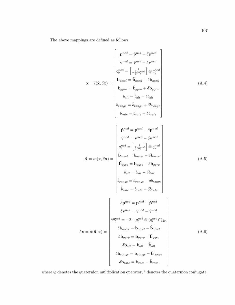
107

The above mappings are defined as follows

x = l(x, δx) =

pned = pned + δpned

vned = vned + δvned

qnedb =[

1− 1

2δθnedb

]⊗ qned

b

baccel = baccel + δbaccel

bgyro = bgyro + δbgyro

balt = balt + δbalt

brange = brange + δbrange

brate = brate + δbrate

(A.4)

x = m(x, δx) =

pned = pned − δpned

vned = vned − δvned

qnedb

=[

112δθnedb

]⊗ qnedb

baccel = baccel − δbaccel

bgyro = bgyro − δbgyro

balt = balt − δbalt

brange = brange − δbrange

brate = brate − δbrate

(A.5)

δx = n(x,x) =

δpned = pned − pned

δvned = vned − vned

δθnedb = −2 · (qnedb ⊗ (qnedb

)∗)2:4

δbaccel = baccel − baccel

δbgyro = bgyro − bgyro

δbalt = balt − balt

δbrange = brange − brange

δbrate = brate − brate

(A.6)

where⊗ denotes the quaternion multiplication operator, ∗ denotes the quaternion conjugate,

108

and the 2 : 4 subscript refers to elements 2 through 4 of the resulting quaternion. All other

variables are defined in the main body of the thesis.

These mappings can be validated to ensure consistency between all three states. To

clarify, this validation step validates the relationships between the states and does not

validate correct implementation of the states themselves. This validation step was performed

on the state vectors in Chapter 3. To perform the validation of the above mappings for the

truth, estimated, and error states, the mappings were programmed into MATLAB, and the

following steps were taken.

1. An initial error state, δx, and an initial truth state x were defined. The error state

was formed using a random number generator. Both the error state and the truth

state are shown in Table A.1.

Table A.1: Defining truth and error state.

Position Velocity Attitude Bias Accel Bias Gyro Bias Alt Bias Range Bias Rate

x (1000,0,-500) (50,0,0) (1,0,0,0) (0.228,0.436,0.311) (0.923,0.430,0.184) 0.905 0.980 0.221

δx (0.379,0.812,0.533) (0.351,0.939,0.876) (0.018,0.021,0.020) (0.208,0.301,0.471) (0.230,0.844,0.195) 0.226 0.171 0.101

2. The initial truth states and error states were fed into the function m(x, δx) to produce

a test estimate state, which is denoted as x′. The result is shown in Table A.2.

Table A.2: Estimated state.

Position Velocity Attitude Bias Accel Bias Gyro Bias Alt Bias Range Bias Rate

x′ (999.621,-0.812,-500.533) (49.649,-0.939,-0.876) (0.999,0.009,0.010,0.010) (0.020,0.135,-0.160) (0.693,-0.414,-0.010) 0.679 0.809 0.120

3. The initial truth state and x′ were fed into the function n(x′,x) to produce a test

error state, which is denoted as δx′. The difference between the initial error state, δx,

and test error state, δx′, was then calculated. This is shown in Table A.3. The result

of the difference was close to zero, which validates the error state mapping.

4. The test estimate state and initial error state were fed into the function l(x′, δx) to

produce a test truth state, which is denoted as x′. The difference between the test

109

Table A.3: Difference between defined error with calculated error.

Position Velocity Attitude Bias Accel Bias Gyro Bias Alt Bias Range Bias Rate

δx (0.379,0.812,0.533) (0.351,0.939,0.876) (0.018,0.021,0.020) (0.208,0.301,0.471) (0.230,0.844,0.195) 0.226 0.171 0.101

δx′ (0.379,0.812,0.533) (0.351,0.939,0.876) (0.018,0.021,0.020) (0.208,0.301,0.471) (0.231,0.844,0.195) 0.226 0.171 0.101

δx− δx′ (0,0,0) (0,0,0) (-0.264e-5,-0.298e-5,-0.281e-5) (0,0,0) (0,0,0) 0 0 0

truth state, x′, and the initial truth state, x, was calculated. This is shown in Table

A.4. The difference was sufficiently close to zero, which validates the truth state

mapping.

Table A.4: Difference between defined truth and calculated truth.

Position Velocity Attitude Bias Accel Bias Gyro Bias Alt Bias Range Bias Rate

x (1000,0,-500) (50,0,0) (1,0,0,0) (0.228,0.436,0.311) (0.923,0.430,0.184) 0.905 0.980 0.221

x′ (1000,0,-500) (50,0,0) (1,0,0,0) (0.228,0.436,0.311) (0.923,0.430,0.184) 0.905 0.980 0.221

x− x′ (0,0,0) (0,0,0) (0,0,0,0) (0,0,0) (0,0,0) 0 0 0

A.2 Truth and Navigation State Propagation and Validation

To verify the consistency of the model definitions, each state propagation model and

measurement model is simulated in MATLAB. For the purposes of this verification step, all

noise sources and biases are set to zero. The simulation then propagates the truth state and

estimated state using the truth model and navigation model, respectively. Without noise,

the truth and navigation models should produce nearly the same results.

This verification step was performed on the models defined in Chapter 3. The simula-

tion was provided with accelerometer and gyroscope data, which moves the model along a

trajectory. In the absence of noise, the sensor data provided to the truth model and navi-

gation model was identical. The trajectory defined by the sensor data is shown in Figure

A.1.

After both models processed the sensor data, errors in position, velocity, and attitude

are calculated using the n(x,x) function defined in Section A.1. The resulting errors were

plotting and are shown in Figure A.2. Notice the scale factor in the upper corner of each

subfigure, which shows that these errors are very close to zero.

110

Fig. A.1: Trajectory of UAV using true measurements from an IMU.

As assumed at the beginning of the simulation, no noise or bias was added to the states

or sensor measurements. Figure A.3 verifies zero bias throughout the simulation.

At each Kalman update time, measurements were taken using the sensor measurement

function z and the estimate measurement function ˆz. The difference between these mea-

surements is called the residual measurement error and is shown in Figure A.4 for the range,

range rate, and altimeter measurements. As with the position, velocity, and attitude errors,

the residual errors are multiplied by a scale factor which produces near zero values for each

measurement residual.

This process validated that the truth model and navigation models from Chapter 3

produce the same results in the absence of noise. In other words, the two models are

consistent with each other.

A.3 Error State Propagation and Validation

This step validates the propagation of the error state. To do this, the error state is

propagated forward in time using a non-linear model and a linear model. The difference

between the non-linear and linear error states should be small.

111

Fig. A.2: Errors in the position, velocity, and attitude between the truth and navigationmodels.

112

Fig. A.3: Errors of the bias states, which are all zero with no noise propagation.

113

Fig. A.4: Residual errors between the true measurements and estimated measurements.

114

The nonlinear error state can be found be propagating the non-linear truth and nav-

igation models forward in time and calculating the error between the two models. This

is done using the already validated n(x,x) mapping. Note that the non-linear truth and

navigation models have also already been validated.

The linear error state is propagated using the linear model defined by the F matrix.

This matrix is developed through linearizing the truth model about the estimated state.

The linear error state at time t is calculated using the F matrix as δx = F δx. The same

initial error used in the nonlinear error propagation is used to initialize the linear error

model. The model is then propagated forward in time for t seconds. This results in a linear

error state at time t.

The nonlinear and linear error states are compared to each other for accuracy. The

F is considered validated is the difference between the nonlinear and linear error states is

“small”1. This validation process was performed on the F matrix from Chapter 3 and the

results are shown in Table A.5.

For this application, the errors are considered small enough. Thus, the linear error

model is validated and is consistent with the definitions of the nonlinear truth and navigation

models.

A.4 Linear Measurement Validation

The difference between z and ˆz is called the measurement “residual” and will be denoted

δz. The residual is important in the EKF to calculate an updated error state vector. The

residual is used in this section to validate the H matrix in the linear measurement model.

For purposes of validation, let δznl to be the nonlinear measurement residual and δzl to be

1The word “small” must be interpreted differently for each new application. In any case, the differencebetween the two error states will be non-zero, because the linear error model does not account for higherorder error terms.

115

Table A.5: Validation of F matrix using a comparison of nonlinear and linear error statesat time t.

state delx linear delx nonlinear propError

px 1.2027 1.202 0.00070823py 2.1446 2.1429 0.0017244pz 3.2835 3.2849 -0.0013857vx 0.30566 0.30424 0.001419vy 0.089675 0.086234 0.0034411vz 0.26791 0.27067 -0.002767θx 0.0099969 0.0099951 1.7465e-06θy 0.020009 0.020006 3.3867e-06θz 0.030013 0.030008 5.3278e-06

baccel,x 0.0080317 0.0080317 0baccel,y 0.016063 0.016063 0baccel,z 0.024095 0.024095 0bgyro,x 3.9693e-06 3.9693e-06 0bgyro,y 7.9386e-06 7.9386e-06 0bgyro,z 1.1908e-05 1.1908e-05 0balt 0.81873 0.81873 0brange 1.6375 1.6375 0brate 1.2281 1.2281 0

the linear measurement residual. These residuals are defined by

δznl = z− ˆz (A.7)

δzl = Hδx (A.8)

In Section A.3, the F matrix was validated by calculating errors using nonlinear propa-

gation and comparing the results with errors calculated using linear propagation. A similar

method can be employed to validate the H matrix. An error, δx is injected into the truth

model. Measurements for z and ˆz are made and an H matrix is calculated. Just as in

validating F , this validation is done in the absence of process and measurement noise.

With values for z, ˆz, and H, the nonlinear residual δznl and the linear residual δzl are

calculated. The two residual measurements are compared with each other. If the difference

between the two residuals is “small” then the H matrix is validated.

This validation step was used on the measurement model from Chapter 3, and the

116

results have been provided. Table A.6 shows the results of the validation process. The

error between the two residual calculations is several orders of magnitude smaller than the

measurements z and ˆz, which are on the order of hundreds of meters. The difference between

the nonlinear and linear residuals is considered small enough in this case. Therefore, the H

matrix in the linear measurement model is validated.

Table A.6: Validation of H matrix by calculating the difference between linear and nonlinearresidual measurements.

residual linear residual nonlinear resError

Range -0.49928 -0.49676 -0.0025155

Range Rate 1.2466 1.2472 -0.00057447

Altitude -2 -2 0

A.5 Covariance Propagation Validation

This section provides details on validating the covariance propagation equations. This

validation step was again applied to the model in Chapter 3. To validate the propagation

of the error state covariance in the presence of noise, the following steps are performed.

• An initial state covariance P (t0) is defined.

• Errors consistent with the initial state covariance are injected into the estimated state

x.

• The matrices F , B, and Q are calculated.

• The covariance is propagated forward in time without Kalman updates.

• The truth state and estimated state are propagated forward in time without Kalman

updates. The error between the truth and estimated states is calculated.

• The propagation of covariance and state vectors repeats several times to perform a

Monte Carlo simulation.

• Hairline plots from the Monte Carlo simulation are created.

117

• 3σ bounds are created from the covariance propagation. If the propagation errors

from the truth and estimated states are contained within the 3σ bounds, then the

covariance propagation is validated.

To begin, an initial state covariance is defined P (t0). The diagonals of P (t0) contain

variances for each error state, denoted σ2δxi

where δxi represents the ith component of the

error state vector. With these variances, P (t0) is equal to,

P (t0) =

σ2δpned

03×3 03×3 03×3 03×3 03×1 03×1 03×1

03×3 σ2δvned

03×3 03×3 03×3 03×1 03×1 03×1

03×3 03×3 σ2δθnedb

03×3 03×3 03×1 03×1 03×1

03×3 03×3 03×3 σ2δbaccel

03×3 03×1 03×1 03×1

03×3 03×3 03×3 03×3 σ2δbgyro

03×1 03×1 03×1

01×3 01×3 01×3 01×3 01×3 σ2δbalt

0 0

01×3 01×3 01×3 01×3 01×3 0 σ2δbrange

0

01×3 01×3 01×3 01×3 01×3 0 0 σ2δbrate

(A.9)

In simulation, values for the error state are set by the user. Table A.7 shows the values

selected for this validation step. These values are in terms of 3σ values, denoted σ3s,δxi .

Table A.7: 3σ values selected by the user for this validation step.

3σ (State) Value

σ3s,δpned diag([1, 1, 3]) (m)

σ3s,δvned diag([0.1, 0.1, 0.1]) (m/s)

σ3s,δθnedbdiag([0.1, 0.1, 0.1]) (rad)

σ3s,δbaccel diag([0.001, 0.001, 0.001]) (g)

σ3s,δbgyro diag([1, 1, 1]) (deg/hr)

σ3s,δbalt 0.1 (m)

σ3s,δbrange 0.1 (m)

σ3s,δbrate 0.1 (m/s)

Errors can be generated using standard normal random variables. Let y ∼ N (0, 1). An

118

error δxi in the error state vector δx can be generated as 2 δxi = yσss,δxi . These δxi errors

are then injected into the initial estimated state x.

Recall the equation for the power spectral density Q.

Q =

σ2vrwI3×3 03×3 03×3 03×3 03×1 03×1 03×1

03×3 σ2arwI3×3 03×3 03×3 03×1 03×1 03×1

03×3 03×32σ2ss,baccelτaccel

I3×3 03×3 03×1 03×1 03×1

03×3 03×3 03×32σ2ss,bgyro

τgyroI3×3 03×1 03×1 03×1

03×3 03×3 03×3 03×32σ2ss,baltτalt

0 0

01×3 01×3 01×3 01×3 02σ2ss,brange

τrange0

01×3 01×3 01×3 01×3 0 02σ2ss,brateτrate

(A.10)

In simulation, each of the noise variances in Q is selected by the user in terms of 3σ values.

The 3σ values used for this validation step are shown in Table A.8.

Table A.8: 3σ noise values used for covariance propagation validation.

3σ (Noise) Values

σ3s,vrw 0.06 (m/s/sqrt(hr))

σ3s,arw 0.07 (deg/sqrt(hr))

σ3s,baccel 0.001 (g)

σ3s,bgyro 1 (deg/hr)

σ3s,balt 0.1 (m)

σ3s,brange 0.1 (m)

σ3s,brate 0.1 (m)

Given the values for the initial covariance P , the injected errors δx, and the power

spectral density Q, a Monte Carlo simulation is run to validate the covariance propagation.

The Monte Carlo simulation was run 200 times. The results of the simulation are given in

Figures A.5 through A.10.

2This is the expression for generating continuous noise. In software, the noise is discrete. To simulate

the discrete samples of a continuous noise process, the actual calculation is δxi = y

√σ23s,δxi∆t

where ∆t is thesimulation sampling rate.

119

Fig. A.5: Hairline plot showing the propagation errors in position. From top to bottom:North position error, east position error, down position error.

120

Fig. A.6: Hairline plot showing the propagation errors in velocity. From top to bottom:North velocity error, east velocity error, down velocity error.

121

Fig. A.7: Hairline plot showing the propagation errors in attitude. From top to bottom:North attitude error, east attitude error, down attitude error.

122

Fig. A.8: Hairline plot showing the propagation errors in accelerometer bias. From top tobottom: X accelerometer bias error, Y accelerometer bias error, Z accelerometer bias error.

123

Fig. A.9: Hairline plot showing the propagation errors in gyroscope bias. From top tobottom: X gyroscope bias error, Y gyroscope bias error, Z gyroscope bias error.

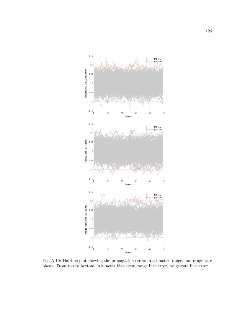
124

Fig. A.10: Hairline plot showing the propagation errors in altimeter, range, and range-ratebiases. From top to bottom: Altimeter bias error, range bias error, range-rate bias error.

125

Each hairline plot shows 3σ error bounds denoted by the dotted lines. These bounds

are calculated using the error state covariance matrix P . Each hair in the hairline plot is a

single run of the Monte Carlo simulation. Because the bounds are 3σ bounds, most of the

hairs should remain in the bounds with the occasional outlier. For 200 runs of the Monte

Carlo simulation, the resulting errors are within bounds. This validates the propagation of

the error state covariance matrix.

A.6 Kalman Update Validation

This section validates the equations from the previous section. Before validation, an

R matrix is selected, which determines the noise variances of the radar and altimeter mea-

surements. For this section, R is equal to

R =

σ2zrange

0 0

0 σ2zrate

0

0 0 σ2zalt

(A.11)

where σzi = σ3s,zi/3 and where the σ3s,zi are selected by the user and are defined in Table

A.9.

Table A.9: Noise standard deviations used for SAR and altimeter measurement noises.

3σ (Measurement) Values

σzradar 0.2 (m)

σzrate 0.2 (m/s)

σzalt 0.2 (m)

If implemented correctly, the Kalman filter should produce residual measurements that

are zero-mean and white. After a single Monte Carlo run, the residual measurements with

their associated covariances were plotted. These plots are shown in Figure A.11. As in

Section A.5, the solid line represents a single Monte Carlo run and the dotted line represents

the 3σ bounds of the measurement residual.

126

Fig. A.11: Residual measurements after implementation of Kalman updates. From top tobottom: Altimeter residual, range residual, range-rate residual.

127

It was observed that the measurement residuals satisfy the zero-mean and white condi-

tions. To further validate correct implementation of the Kalman update equations, a Monte

Carlo simulation with 200 runs was performed. Hair plots of the propagation error were

created as was done in Section A.5. These plots are shown in Figures A.12 through A.17.

Note how the covariance of the error state (indicated by the dotted line) changes in tandem

with the actual state errors. This further implies correct implementation.

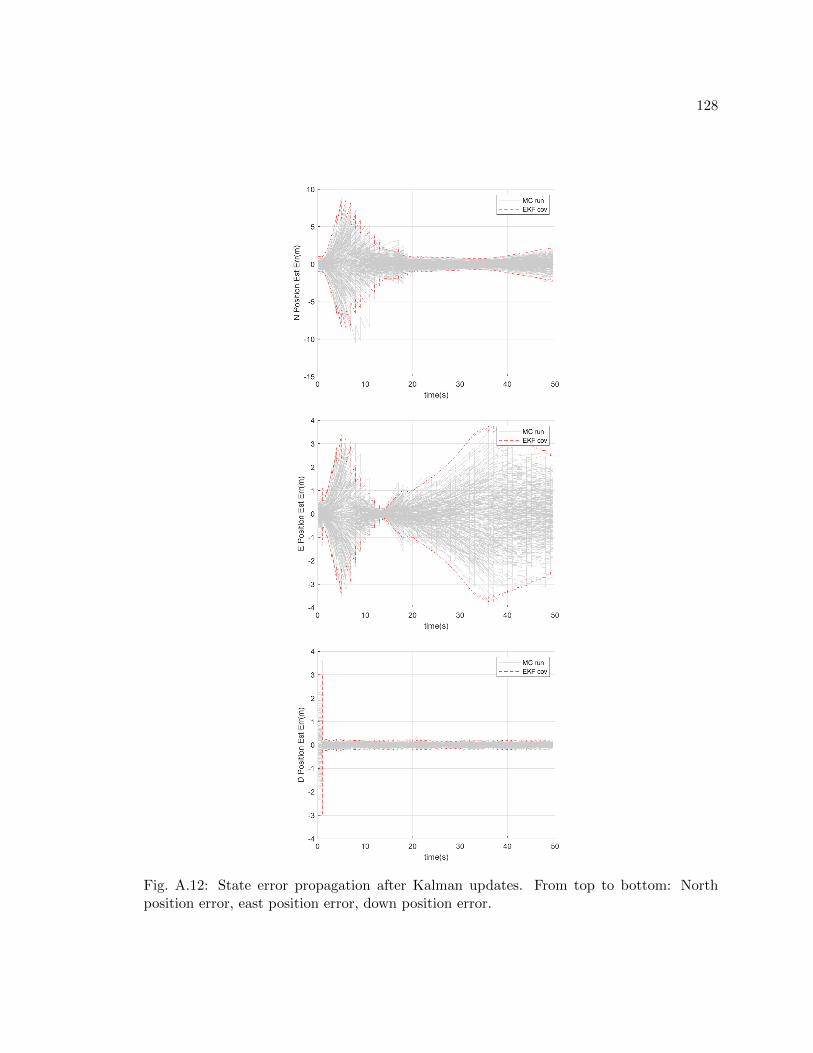
128

Fig. A.12: State error propagation after Kalman updates. From top to bottom: Northposition error, east position error, down position error.

129

Fig. A.13: State error propagation after Kalman updates. From top to bottom: Northvelocity error, east velocity error, down velocity error.

130

Fig. A.14: State error propagation after Kalman updates. From top to bottom: Northattitude error, east attitude error, down attitude error.

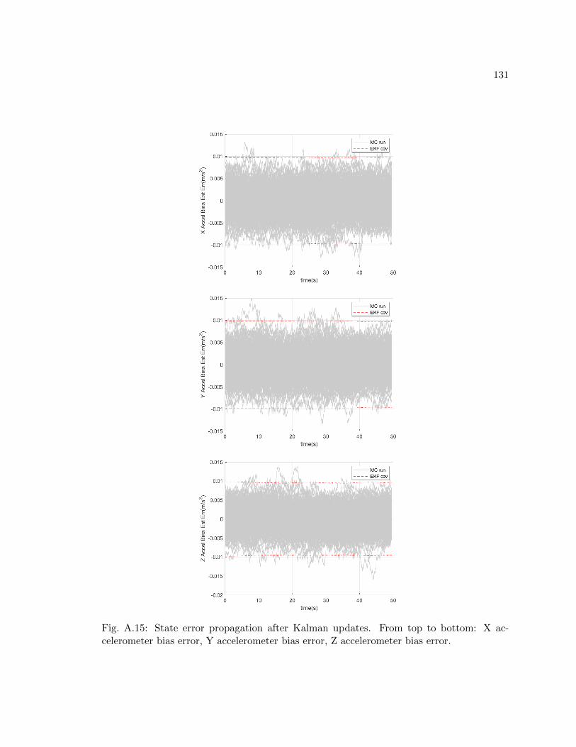
131

Fig. A.15: State error propagation after Kalman updates. From top to bottom: X ac-celerometer bias error, Y accelerometer bias error, Z accelerometer bias error.

132

Fig. A.16: State error propagation after Kalman updates. From top to bottom: X gyroscopebias error, Y gyroscope bias error, Z gyroscope bias error.

133

Fig. A.17: State error propagation after Kalman updates. From top to bottom: Altimeterbias error, range, range-rate bias error.

134

APPENDIX B

EKF Related Derivations

This section contains derivations for portions of the EKF used in Chapters 3 and 5.

B.1 Linearization of Velocity State

The linearized velocity state arises when linearizing the truth state about the estimated

state to form a linear error model. The linearization process begins with

˙vned

+ δvned = (I − (δθnedb ×))Rnedb

(νb − baccel − δbaccel − nν) + gned (B.1)

The goal is to write an expression for the linear error model, δv. Expanding the

equation produces

˙vned

+δvned = Rnedb

(νb−baccel−δbaccel−nν)−(δθnedb ×)Rnedb

(νb−baccel−δbaccel−nν) (B.2)

Subtracting the estimated state and reversing the order of the cross product results in

δvned = Rnedb

(−δbaccel − nν) + [Rnedb

(νb − baccel − δbaccel − nν)]× δθnedb (B.3)

Neglecting second order terms results in the expression used in the linear error model

in Chapters 3 and 5.

δvned =Rnedb

(−δbaccel − nν) + [Rnedb

(νb − baccel)]× δθnedb

=[Rnedb

(νb − baccel)]× δθnedb −Rnedbδbaccel −Rnedb

nν) (B.4)

135

B.2 Linearization of Attitude State

The linearized attitude state again arises from linearizing the truth state to produce a

linear error model. The process begins with

d

dt

([1

− 12δθnedb

]⊗ qned

b

)=

1

2

[1

− 12δθnedb

]⊗ qned

b⊗[

0ωb−bgyro−δbgyro−nω

](B.5)

For clarity, let δq =[

1− 1

2δθnedb

]. This results in,

d

dt(δq ⊗ qned

b) =

1

2δq ⊗ qned

b⊗[

0ωb−bgyro−δbgyro−nω

](B.6)

Expanding the derivative on the left and splitting the quaternion on the right results

in

δq ⊗ qnedb

+ δq ⊗ qnedb

=1

2δq ⊗ qned

b⊗([

0ωb−bgyro

]+[

0−δbgyro−nω

])(B.7)

Distributing the quaternion multiplication on the right results in

δq ⊗ qnedb

+ δq ⊗ qnedb

=1

2δq ⊗ qned

b⊗[

0ωb−bgyro

]+

1

2δq ⊗ qned

b⊗[

0−δbgyro−nω

](B.8)

Recall from Chapters 3 and 5 that the expression for attitude in the navigation model

is qnedb

= qnedb⊗ 1

2

[0

ωb−bgyro

]Substituting in the estimated attitude state results in

δq ⊗ qnedb

+ δq ⊗ qnedb

= δq ⊗ qnedb

+1

2δq ⊗ qned

b⊗[

0−δbgyro−nω

](B.9)

A δq ⊗ qnedb

term appears on both sides of the equation and can be cancelled.

δq ⊗ qnedb

=1

2δq ⊗ qned

b⊗[

0−δbgyro−nω

](B.10)

Right hand multiplication by (qnedb

)∗ on both sides results in

δq =1

2δq ⊗ qned

b⊗[

0−δbgyro−nω

]⊗ (qned

b)∗ (B.11)

136

The last three terms of this equation are of the form of a quaternion rotation. Expressed

in the language of rotation matrices, the quaternion rotation portion of the equation can

be written as,

qnedb⊗[

0−δbgyro−nω

]⊗ (qned

b)∗ =⇒

[0

−Rnedb

δbgyro−Rnedb

nω

](B.12)

It follows,

δq =1

2δq ⊗

[0

−Rnedb

δbgyro−Rnedb

nω

](B.13)

Recall δq =[

1− 1

2δθnedb

]. Substituting this expression back into the equation results in

[1

− 12δθnedb

]=

1

2

[1

− 12δθnedb

]⊗[

0−Rned

bδbgyro−Rned

bnω

](B.14)

Recall that quaternion multiplication for two quaternions [ rs ] and [ qt ] is equal to[rq−s·t

rt+qs+s×t

]Using this definition,

[1

− 12δθnedb

]=

1

2

[1

− 12δθnedb

]⊗[

0−Rned

bδbgyro−Rned

bnω

]=

1

2

[− 1

2δθnedb ·(−Rned

bδbgyro−Rned

bnω)

− 12δθnedb ×(−Rned

bδbgyro−Rned

bnω)−Rned

bδbgyro−Rned

bnω

](B.15)

Equating the vector portion of the quaternion results in

−1

2δθnedb =

1

2(−1

2δθnedb × (−Rned

bδbgyro −Rnedb

nω)−Rnedbδbgyro −Rnedb

nω)

δθnedb =1

2δθnedb × (−Rned

bδbgyro −Rnedb

nω) +Rnedbδbgyro +Rned

bnω (B.16)

Neglecting second order terms results in the expression used in the linear error model

in Chapters 3 and 5.

δθnedb = Rnedbδbgyro +Rned

bnω (B.17)

137

B.3 Linearization of Measurement Model

To obtain the H matrix, the measurement model is linearized using the Jacobian.

Recall that the measurement model z is defined as

z =

zrange

zrate

zalt

=

||r− pned||+ brange + nrange

−(vned)T r−pned||r−pned|| + brate + nrate

−pz + balt + nalt

(B.18)

The Jacobian of the measurement model evaluated at x is equal to,

H =δz

δx

∣∣∣∣x=x

H =

δzrangeδpned

δzrangeδvned

δzrangeδθned

δzrangeδbaccel

δzrangeδbgyro

δzrangeδbalt

δzrangeδbrange

δzrangeδbrate

δzrateδpned

δzrateδvned

δzrateδθned

δzrateδbaccel

δzrateδbgyro

δzrateδbalt

δzrateδbrange

δzrateδbrate

δzaltδpned

δzaltδvned

δzaltδθned

δzaltδbaccel

δzaltδbgyro

δzaltδbalt

δzaltδbrange

δzaltδbrate

∣∣∣∣∣x=x

(B.19)

Notice that many of the partial derivatives will equal 0, as the measurements do not

contain several of the terms in δx. The list of nonzero partial derivatives is

δzrangeδpned

,δzrateδpned

,δzrateδvned

,δzaltδpned

,δzrangeδbrange

,δzrateδbrate

, andδzaltδbalt

Using the regular rules for derivatives (i.e. chain rule, quotient rule, etc) the nonzero

partial derivatives are calculated in order.

The partial derivative of the range with respect to position:

δzrangeδpned

=δ

δpned(||r− pned||+ brange + nrange)

=δ

δpned(√

(r− pned)T (r− pned) + brange + nrange)

=

(1/2√

(r− pned)T (r− pned)

)(−2(r− pned)T )

=−(r− pned)T

||r− pned||(B.20)

138

The partial derivative of the range rate with respect to position:

δzrateδpned

=δ

δpned(−(vned)T

r− pned

||r− pned||+ brate + nrate)

=δ

δpned(−(vned)T

r− pned√(r− pned)T (r− pned)

)

=

√(r− pned)T (r− pned)(vned)T

(r− pned)T (r− pned)

−(−vned)T (r− pned)

(1/2√

(r−pned)T (r−pned)

)(−2(r− pned)T )

(r− pned)T (r− pned)

=||r− pned||(vned)T − (vned)T (r− pned)

((r−pned)T

||r−pned||

)||r− pned||2

=(vned)T

||(r− pned)||− (vned)T (r− pned)(r− pned)T

||(r− pned)||3(B.21)

The partial derivative of the range rate with respect to velocity:

δzrateδvned

=δ

δvned(−(vned)T

r− pned

||r− pned||+ brate + nrate)

=δ

δvned(−(vned)T

r− pned

||r− pned||)

=−(r− pned)T

||r− pned||(B.22)

The partial derivative of the altitude with respect to the position:

δzaltδpned

=δ

δpned(−pz + balt + nalt)

=δ

δpned(−pz)

= [0, 0,−1] (B.23)

139

The partial derivative of the range with respect to the radar range bias:

δzrangeδbrange

=δ

δbrange(||r− pned||+ brange + nrange)

=δ

δbrange(brange)

= 1 (B.24)

The partial derivative of the range rate with respect to the range-rate bias:

δzrateδbrate

=δ

δbrate(−(vned)T

r− pned

||r− pned||+ brate + nrate)

=δ

δbrate(brate)

= 1 (B.25)

The partial derivative of the altitude with respect to the altimeter bias:

δzaltδbalt

=δ

δbalt(−pz + balt + nalt)

=δ

δbalt(balt)

= 1 (B.26)

Populating the Jacobian with the above partial derivatives and evaluating at x = x

yields

H =

−(r−pned)T

||r−pned|| 01x3 01x3 01x3 0 1 0

(vned)T

||(r−pned)|| −(vned)T (r−pned)(r−pned)T

||(r−pned)||3−(r−pned)T

||(r−pned)|| 01x3 01x3 0 0 1

[0, 0,−1] 01x3 01x3 01x3 1 0 0

(B.27)

140

Let d = r− pned to obtain the H matrix from Chapters 3 and 5.

H =

−dT||d|| 01x3 01x3 01x3 01x3 0 1 0

(vned)T

||d|| −(vned)TddT

||d||3−dT||d|| 01x3 01x3 01x3 0 0 1

[0, 0,−1] 01x3 01x3 01x3 01x3 1 0 0

(B.28)

141

APPENDIX C

Pulse Compression Derivation

This appendix derives the expression used for a pulse compressed signal after matched

filtering. A commonly used signal for pulse compression in radar is a linear frequency

modulated (LFM) pulse, or a chirp pulse. This pulse signal is sinusoid like with a phase

component that is quadratic in time. The LFM pulse is denoted s(t) and is of the form

s(t) =

exp(j2πf0t+ jαt2), 0 ≤ t ≤ T

0, otherwise

(C.1)

where f0 is the initial frequency, α is related to the linear FM rate, 1 and T is the

pulse duration. Figure C.1 shows the real and imaginary parts of a chirp signal gener-

ated in MATLAB. Notice in Figure C.2 that the phase of the signal is quadratic, and the

instantaneous frequency of the signal is linear with slope α/π.

To compress the linear FM pulse, a matched filter is used, which is a time reversed,

conjugate version of s(t). The matched filter result is denoted p(t) and is defined as the

convolution of s(t) with the matched filter s∗(T − t).

p(t) = s(t) ∗ s∗(T − t)

=

∫ t

0 s(λ)s∗(T − (t− λ))dλ, 0 ≤ t ≤ T∫ Tt−T s(λ)s∗(T − (t− λ))dλ, T ≤ t ≤ 2T

(C.2)

The convolution is split into two integrals. The first of the two integrals is solved as

1In other places in this thesis, K is used to denote the FM rate. The conversion between K and α isα = πK

142

Fig. C.1: Real (left) and imaginary (right) transmission of pulse s(t).

Fig. C.2: Phase (left) and instantaneous frequency (right) of s(t).

143

∫ t

0s(λ)s∗(T − (t− λ))dλ =

∫ t

0s(λ)s∗(λ+ T − t)dλ

=

∫ t

0ej(2πf0t+αt2)e−j(2πf0(λ+T−t)+α(λ+T−t)2)dλ

=

∫ t

0e−j(2πf0(T−t)+α(T−t)2+2αλ(T−t))dλ

= e−j(2πf0(T−t)+α(T−t)2)

∫ t

0e−j2αλ(T−t)dλ (C.3)

Ignoring the constant exponential out front, and by letting ρ = T − t,

∫ t

0e−j2αλρdλ =

e−j2αλρ

−j2αρ

∣∣∣∣t0

=1

−j2αρ[e−j2αtρ − 1

]=e−jαtρ

−j2αρ[e−jαtρ − ejαtρ

](C.4)

Recall the identity sin θ = ejθ−e−jθ2j . Using this identity,

e−jαtρ

−j2αρ[e−jαtρ − ejαtρ

]= e−jαtρ

sin(αtρ)

αρ(C.5)

Returning the constant out front, the expression for the first integral for matched

filtering is,

p(t) = e−j(2πf0ρ+αρ2+αtρ) sin(αtρ)αρ 0 ≤ t < T (C.6)

The second integral in the convolution is identical to the first up to the point of eval-

uating the integrated function at the limits of integration. Once again, the constant out

front is ignored until the end of the derivation.

144

∫ T

t−Te−j2αλρdλ =

e−j2αλρ

−j2αρ

∣∣∣∣Tt−T

=1

−j2αρ[e−j2αtρ − e−j2αtρej2αTρ

]=e−jαtρ

−j2αρ

[e−j(αtρ−2αTρ) − ej(αtρ−2αTρ)

]= e−jαtρ

sin(αρ(2T − t))αρ

(C.7)

Replacing the constant out front, the expression for the second stage of the convolution

is,

p(t) = e−j(2πf0ρ+αρ2+αtρ) sin(αρ(2T−t))αρ T < t < 2T (C.8)

Taking a limit at t = T , p(t) can be written as the following piecewise function.

p(t) = e−j(2πf0ρ+αρ2+αtρ)

sin(αρt)αρ , 0 ≤ t < T

T, t = T

sin(αρ(2T−t))αρ , T < t ≤ 2T

(C.9)

This expression can be written in a closed form using the triangle function tri(x) =

rect(x/2)(1− |x|) and the sinc function sinc(x) = sin(πx)/πx.

p(t) = e−j(2πf0ρ+αρ2+αtρ)(T − |t− T |)sinc(αρ

π(T − |t− T |)) (C.10)

Figure C.3 shows the matched return signal p(t). As a side note, matched filtering pro-

duces good results in the presence of noise. Figure C.4 shows the result of pulse compression

on a signal with an SNR or -15dB.

145

Fig. C.3: Matched return signal p(t).

Fig. C.4: Transmitted pulse with SNR of -15dB and the matched return signal

146

APPENDIX D

Autofocus

This appendix is meant to give details on autofocusing algorithms explored through

the course of this thesis. The material here is very loosely based on material from [3].

D.1 Range and Range Rate Measurements

In Chapter 3, it was shown that GPS denied navigation was feasible when provided

with range and range rate measurements from a radar system. Later in Chapter 5, it was

stated that these measurements could not be accurately extracted from SAR images. As

a result, range and range rate measurements were replaced with range and cross range

measurements. This section documents the reasoning behind that choice.

The method explored to extract range and range rate measurements from SAR im-

ages hinges on the hyperbolic range equation and its involvement in the backprojection

summation. The hyperbolic range equation is defined as,

R(η) =√R2

0 + V 2r η

2 (D.1)

where R0 is the range of closest approach between the ground target and the radar platform,

Vr is the forward velocity of the radar platform (r subscript refers to rectilinear coordinate

frame), and η is azimuth time. The target on the ground is used as a reference point

from which measurements are taken. The location of the target is assumed to be known.

Furthermore, the backprojection equation is defined as,

A(xpix) =∑n

sout(tpix,n)exp{j4πR(η)

λ} (D.2)

where xpix is the location of an image pixel on the ground, n is used to denote the nth range

compressed signal, λ is the center frequency of the radar’s chirp signal, and sout(tpix,n) is a

147

sample of range compressed data at time tpix,n.

Note that the hyperbolic range equation is expressed as R(η). The range equation as

defined is not explicitly a function of xpix but does depend implicitly on the pixel location.

Both the time of closest approach, η0, and range of closest approach, R0, will change when

xpix changes.

Measuring the range and range rate is a matter of accurately estimating the range

of closest approach, the time of closest approach, and the forward velocity from the SAR

data. After obtaining estimates for each of those parameters, the range is found using the

hyperbolic range equation. The range rate is found using the derivative of the hyperbolic

range equation, which is equal to

dR(η)

d(η)=d(√R2

0 + V 2r η

2)

d(η)

= 2V 2r η

1

2√R2

0 + V 2r η

2

=V 2r η

R(η)(D.3)

By convention, η is centered around the time of closest approach η0. If η0 is known,

extrapolating to other times is simple. Assuming the SAR image is time-stamped and that

the location of the radar ground target is known, R0 and η0 is simple to find by comparing

the true target location to the target location on the SAR image.

This can be done using a cross correlation between a reference image and the resulting

image. The peak of the cross correlation shows how much the target has shifted from

the reference, which can be translated into range of closest approach and time of closest

approach via the range resolution and pulse repetition frequency.

Estimating the range and time of closest approach using the cross correlation was

found to be very accurate. However, estimations of the forward velocity, Vr, proved to be

inaccurate. The method to estimate forward velocity from the SAR image depends on the

phase component of the backprojection equation. This phase component represents the

matched filter portion of azimuth compression. If there are errors in the matched filter

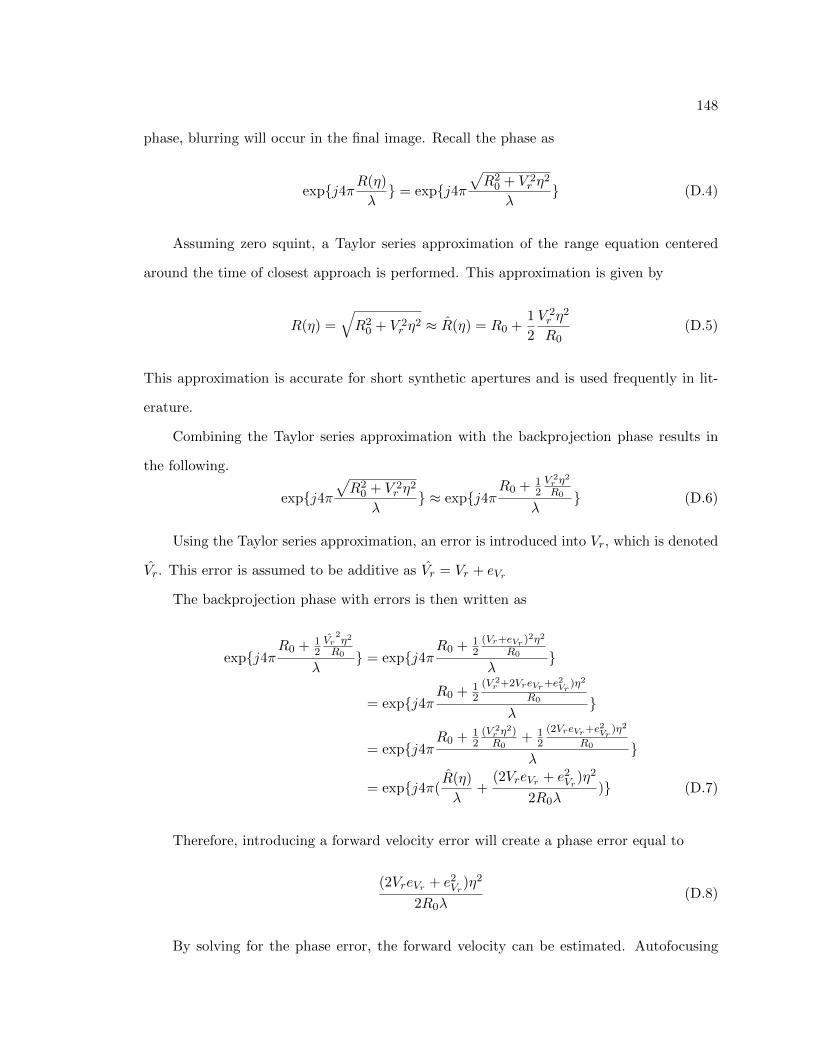
148

phase, blurring will occur in the final image. Recall the phase as

exp{j4πR(η)

λ} = exp{j4π

√R2

0 + V 2r η

2

λ} (D.4)

Assuming zero squint, a Taylor series approximation of the range equation centered

around the time of closest approach is performed. This approximation is given by

R(η) =√R2

0 + V 2r η

2 ≈ R(η) = R0 +1

2

V 2r η

2

R0(D.5)

This approximation is accurate for short synthetic apertures and is used frequently in lit-

erature.

Combining the Taylor series approximation with the backprojection phase results in

the following.

exp{j4π√R2

0 + V 2r η

2

λ} ≈ exp{j4π

R0 + 12V 2r η

2

R0

λ} (D.6)

Using the Taylor series approximation, an error is introduced into Vr, which is denoted

Vr. This error is assumed to be additive as Vr = Vr + eVr

The backprojection phase with errors is then written as

exp{j4πR0 + 1

2Vr

2η2

R0

λ} = exp{j4π

R0 + 12

(Vr+eVr )2η2

R0

λ}

= exp{j4πR0 + 1

2

(V 2r +2VreVr+e2Vr )η2

R0

λ}

= exp{j4πR0 + 1

2(V 2r η

2)R0

+ 12

(2VreVr+e2Vr )η2

R0

λ}

= exp{j4π(R(η)

λ+

(2VreVr + e2Vr

)η2

2R0λ)} (D.7)

Therefore, introducing a forward velocity error will create a phase error equal to

(2VreVr + e2Vr

)η2

2R0λ(D.8)

By solving for the phase error, the forward velocity can be estimated. Autofocusing

149

techniques are used to correct for the phase errors. If autofocusing is successful, the phase

of the matched filter could be adjusted to equal

exp{j4π(R(η)

λ+ (

(2VreVr + e2Vr

)

2R0λ+ cauto)η

2)} (D.9)

where cauto is a correction factor resulting from the autofocusing. Assuming an accurate

autofocus result,(2VreVr+e2Vr )

2R0λ+ cauto = 0 is true and VR can be solved for.

To simplify the expression, the e2Vr

term is typically small enough to ignore. As such,

an expression for a forward velocity estimate is

Vr = −cautoR0λ

eVr(D.10)

The above equation depends on eVr , which is problematic since the velocity error can-

not be exactly known. However, the greater problem of this expression is cauto, which in

simulation was never accurate enough to properly estimate Vr even when velocity errors

were perfectly known. In most cases, the Kalman filter produces a better estimate of Vr;

however, using the Kalman filter’s velocity estimate did not produce accurate range rate

measurements and led to diverging estimation errors. As a result of these discoveries, the

structure of the measurement model was changed to incorporated range and cross range

measurements.

D.2 Autofocus

This section provides information on two of the autofocusing methods explored for

this thesis. These methods are contrast maximization and azimuth misregistration. Other

methods not explored here include phase difference (PD) and phase gradient algorithm

(PGA).

Contrast maximization and azimuth misregistration were both implemented in order

to compare estimation accuracy of forward velocity. However, as mentioned above, neither

algorithm was able to produce accurate estimates of the forward velocity. In comparison

150

to each other, azimuth misregistration was more accurate than contrast maximization;

however, in both cases, the velocity estimate was worse than the estimate provided by the

EKF.

Contrast Maximization

Contrast maximization essentially adjusts the phase in the azimuth matched filter until

the contrast in the image has been maximized. This is an iterative process, but the iteration

number may be cut down through the aid of quadratic approximation. Essentially, measures

of contrast are approximately quadratic around the correct answer.

There are several different measures for the contrast of an image. Three have been

tested on simulation data. Two of the three metrics seem to yield accurate results.

The first measure is the average pixel intensity to power ratio. It is calculated as

C =E[|I|2]

E[|I|]2(D.11)

where E[·] is the expectation operator and |I| is the pixel magnitude. This metric appeared

to yield correct results. This measure was proposed in [3].

The second measure is the standard deviation to average magnitude ratio. It is calcu-

lated as

C =

√E[|I|2]− E[|I|]2

E[|I|](D.12)

This metric also appears to give good results. This measure was proposed in [57].

The third measure is the standard deviation to average pixel intensity. It is calculated

as

C =

√E[|I|2]− E[|I|]2

E[|I|2](D.13)

This metric did not seem to give correct results. When the image was correctly focused,

this metric yielded a result that was lower than when the image was incorrectly focused.

This measure was also proposed in [57].

151

To solve for the optimal cauto value, a diminishing step size gradient descent optimiza-

tion structure was implemented. This required the gradient of the Contrast with respect

to cauto. This expression is complicated enough that no analytical solution was solved for.

Instead, a numerical derivative was used.

Figures D.1 and D.2 are provided as a demonstration of the autofocusing algorithm’s

effectiveness. In Figure D.1, the left most image is a reference image showing the target

formed with the true trajectory. The middle image is the result of forming an image with

an along track velocity error. The right most image is result of the autofocusing algorithm

that takes the blurred image as input.

Contrast maximization is an iterative algorithm, so Figure D.2 has been provided to

show how the values for contrast and cauto change with respect to the iterations of the

optimization routine. The left most plot shows the contrast using the intensity over power

ratio. The right most image shows the convergence of cauto.

Azimuth Misregistration

Azimuth misregistration is based on multilook processing. The idea is that an error in

the azimuth FM rate will cause a ground target to shift in the azimuth direction between

two separate looks of the same target.

In this section the azimuth matched filter is expressed in terms of R0 and Vr.

exp{j4πR0 + 1

2V 2r η

2

R0

λ} (D.14)

By neglecting the constant phase term and defining the azimuth FM rate as Ka = 2V 2r

R0λ,

the azimuth matched filter can be expressed as

exp{jπKaη2} (D.15)

Let Kamf be the azimuth FM rate with an error included such that Kamf = Ka + ∆K

where ∆K is the amount of error present in Kamf .

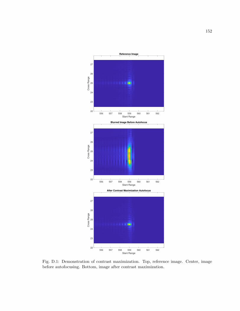
152

Reference Image

556 557 558 559 560 561 562

Slant Range

22

23

24

25

26

27

Cro

ss R

an

ge

Blurred Image Before Autofocus

556 557 558 559 560 561 562

Slant Range

22

23

24

25

26

27

Cro

ss R

an

ge

After Contrast Maximization Autofocus

556 557 558 559 560 561 562

Slant Range

22

23

24

25

26

27

Cro

ss R

an

ge

Fig. D.1: Demonstration of contrast maximization. Top, reference image. Center, imagebefore autofocusing. Bottom, image after contrast maximization.

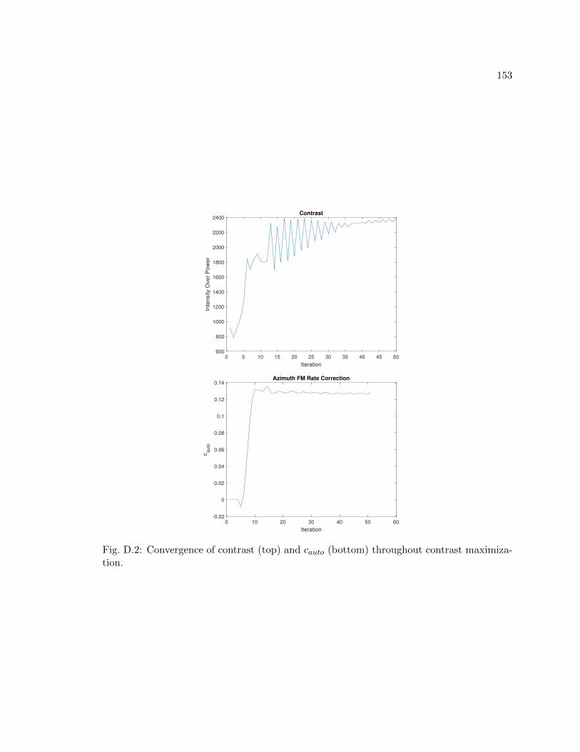
153

0 5 10 15 20 25 30 35 40 45 50

Iteration

600

800

1000

1200

1400

1600

1800

2000

2200

2400

Inte

nsity O

ve

r P

ow

er

Contrast

0 10 20 30 40 50 60

Iteration

-0.02

0

0.02

0.04

0.06

0.08

0.1

0.12

0.14

ca

uto

Azimuth FM Rate Correction

Fig. D.2: Convergence of contrast (top) and cauto (bottom) throughout contrast maximiza-tion.

154

The amount of misregistration between the two separate looks is denoted ∆η and is

defined as

∆η = −∆fa

(1

Ka− 1

Kamf

)(D.16)

For each of the looks, a different frequency band is used in the matched filter. In general,

the frequency used in the matched filter is equal to fη = −Kaη where η is centered around

the time of closest approach. Each of the two looks will have a different center frequency,

denoted fη,1 and fη,2. ∆fa is defined as the difference between the center frequencies of the

two looks, ∆fa = fη,2 − fη,1

By rearranging equation (D.16), the azimuth FM rate error can be expressed as

∆Ka ≈ −K2amf

∆fa∆η (D.17)

∆η can be solved for numerically by cross correlating Look 1 and Look 2 with each

other. the peak of the cross correlation shifts according to the level of misregistration.

Interpolating in azimuth may yield a better misregistration result.

With ∆K solved for, the corrected azimuth matched filter is equal to

exp{jπ(Kamf −∆K)η2} (D.18)

At this point, the ∆K term is converted into a cauto type term for estimation of forward

velocity.

Figures D.3 and D.4 are provided to demonstrate autofocusing using azimuth misreg-

istration. Figure D.3 shows two different looks of the same target. This demonstrates how

the target will shift in azimuth between two looks. The left and center images are the two

looks. The right most image is the cross correlation of the two looks. This shows how the

shift can be tracked using the peak of the cross correlation.

Figure D.4 demonstrates azimuth misregistration. The left most image is a reference

image of the target formed using the true trajectory. The center image an image formed

155

with an along track velocity error. The right most image is the result of autofocusing using

azimuth misregistration.

156

Look 1

554 556 558 560 562 564

Slant Range

20

21

22

23

24

25

26

27

28

29

Cro

ss R

an

ge

Look 2

554 556 558 560 562 564

Slant Range

20

21

22

23

24

25

26

27

28

29

Cro

ss R

an

ge

Cross Correlation Between Look 1 and Look 2

10 20 30 40 50 60 70 80 90

10

20

30

40

50

60

70

80

90

Fig. D.3: Demonstration of misregistration between different looks. Top, look 1. Center,look 2. Bottom, cross correlation between the two looks.

157

Reference Image

556 557 558 559 560 561 562

Slant Range

22

23

24

25

26

27

Cro

ss R

an

ge

Blurred Image Before Autofocus

556 557 558 559 560 561 562

Slant Range

22

23

24

25

26

27

Cro

ss R

an

ge

After Azimuth Misregistration Autofocus

556 557 558 559 560 561 562

Slant Range

22

23

24

25

26

27

Cro

ss R

an

ge

Fig. D.4: Demonstration of autofocusing using azimuth misregistration. Top, referenceimage. Center, image before autofocusing. Bottom, image after azimuth misregistrationautofocusing.

158

APPENDIX E

Spatial Variance and Ambiguities

This appendix is meant to provide discussion on aspects of SAR that require additional

consideration.

Creating images using SAR is not a spatially invariant problem, which poses unique

problems for future study. In this thesis, only single point targets have been considered in

analysis. While easier to conceptualize, the single target scenario does not account for some

behaviors. Errors in image formation or navigation state do not affect each target the same.

For example, if the SAR platform has an error in elevation position, closer targets will be

affected more dramatically than further targets. This is illustrated by Figure E.1. In this

Figure, the solid lines represent the slant range to the targets before error. The dotted lines

represent the slant range after an elevation error is introduced. The bold line superimposed

on the dotted line shows the difference in slant range between the error free case and the

error present case. Notice that the bold line is longer for the closer of the two targets.

Fig. E.1: Illustration of how an elevation error on the slant range affect two distinct targetsdifferently.

Another example of how errors affect multiple targets differently can be seen in Figure

E.2. This figure depicts a velocity error, which appears as a linearly increasing deviation

159

from the true path. In the figure, two targets are show that originally have equal ranges

of closest approach. After a velocity error, the ranges of closest approach change such that

the lengths are no longer equal. Each new range of closest approach depends on the time

at which the error was introduced and the target’s position relative to the radar vehicle’s

position.

Fig. E.2: Illustration of how a velocity error can affect the range of closest approach formultiple targets. Solid black lines indicate truth. Lighter gray lines indicate errors.

Another consideration to be aware of during SAR imaging is the presence of ambiguity.

Ambiguity was discussed in Chapter 3 where it was explained how different combinations

of range and elevation values can lead to equal range values. This is once again illustrated

in Figure E.3. This type of ambiguity can make it difficult to infer navigation errors from

a target’s location within an image.

This ambiguity also exists in the reverse direction. For a given radar platform position,

160

Fig. E.3: Illustration of how combinations of elevation and cross-track errors maintainconstant slant range to a target.

there is an entire continuum of elevations at which a target can be imaged in focus. Focusing

a target at the wrong elevation will cause a cross track shift in the target’s location. This

is illustrated in Figure E.4. This type of ambiguity becomes a problem when knowledge of

the local terrain map is inaccurate. Therefore, errors in the DTED will result in targets

shifted from their true positions.

The goal of the entire thesis is to perform GPS denied navigation using SAR imagery.

In Chapter 4 an analysis is performed that explored the relationship of navigation errors to

SAR imaging errors. That analysis is a stepping stone to inferring navigation errors from

image errors. Another step for future research is to account for the ambiguities explained

above. One potential method of resolving ambiguities in the presence of error is to account

for multiple targets and track how errors effect each target differently. This may lead to

successful navigation error inference using SAR imaging errors.

161

Fig. E.4: Illustration of how a single point target can be focused along a continuum ofelevation and cross track locations.

162

APPENDIX F

Copyright Information

The papers comprising the main body of this thesis have been either published, sub-

mitted for publication, or are soon to be submitted for publication. They are therefore

subject to special copyright statements, which are provided here in this appendix.

The IEEE does not require individuals working on a thesis to obtain a formal reuse

license. In reference to IEEE copyrighted material, which is used with permission in this the-

sis, the IEEE does not endorse any of Utah State University’s products or services. Internal

or personal use of this material is permitted. If interested in reprinting/republishing IEEE

copyrighted material for advertising or promotional purposes or for creating new collective

works for resale or redistribution, please go to http://www.ieee.org/publications standards

/publications/rights/rights link.html to learn how to obtain a License from RightsLink.

F.1 Published Works

©2020 IEEE. Reprinted, with permission, from C. Lindstrom, R. Christensen, and J.

Gunther, “An Investigation of GPS-Denied Navigation Using Airborne Radar Telemetry,”

IEEE/ION Position, Location and Navigation Symposium (PLANS), Apr. 2020.

F.2 Works Submitted for Publication

The following work has been submitted to the IEEE for possible publication. Copy-

right may be transferred without notice. After publication, the afore mentioned terms on

reprinting and republishing of IEEE copyrighted material will apply.

C. Lindstrom, R. Christensen, and J. Gunther, “Sensitivity of BPA SAR Image Forma-

tion to Initial Position, Velocity, and Attitude Navigation Errors,” arXiv:2009.10210 [eess],

Sept. 2020. arXiv: 2009.10210.

163

The material comprising Chapter 5 is currently under revision to be submitted for

publication at a future date. Special copywrite permissions may apply.