a spectral algorithm for latent junction trees
TRANSCRIPT
A Spectral Algorithm for Latent Junction Trees
Ankur P. ParikhCarnegie Mellon University
Le SongGeorgia Tech
Mariya IshtevaGeorgia Tech
Gabi TeodoruGatsby Unit, UCL
Eric P. XingCarnegie Mellon University
Abstract
Latent variable models are an elegant frame-work for capturing rich probabilistic depen-dencies in many applications. However, cur-rent approaches typically parametrize thesemodels using conditional probability tables,and learning relies predominantly on localsearch heuristics such as Expectation Max-imization. Using tensor algebra, we pro-pose an alternative parameterization of latentvariable models (where the model structuresare junction trees) that still allows for com-putation of marginals among observed vari-ables. While this novel representation leadsto a moderate increase in the number of pa-rameters for junction trees of low treewidth,it lets us design a local-minimum-free algo-rithm for learning this parameterization. Themain computation of the algorithm involvesonly tensor operations and SVDs which canbe orders of magnitude faster than EM al-gorithms for large datasets. To our knowl-edge, this is the first provably consistent pa-rameter learning technique for a large classof low-treewidth latent graphical models be-yond trees. We demonstrate the advantagesof our method on synthetic and real datasets.
1 Introduction
Latent variable models such as Hidden Markov Models(HMMs) (Rabiner & Juang, 1986), and Latent Dirich-let Allocation (Blei et al., 2003) have become a popularframework for modeling complex dependencies amongvariables. A latent variable can represent an abstractconcept (such as topic or state), thus enriching thedependency structure among the observed variableswhile simultaneously allowing for a more tractablerepresentation. Typically, a latent variable model isparameterized by a set of conditional probability ta-bles (CPTs) each associated with an edge in the la-
tent graph structure. For instance, an HMM can beparametrized compactly by a transition probability ta-ble and an observation probability table. By summingout the latent variables in the HMM, we obtain a fullyconnected graphical model for the observed variables.
Although the parametrization of latent variable mod-els using CPTs is very compact, parameters in thisrepresentation can be difficult to learn. Compared toparameter learning in fully observed models which iseither of closed form or convex (Koller & Friedman,2009), most parameter learning algorithms for latentvariable models resort to maximizing a non-convex ob-jective via Expectation Maximization (EM) (Demp-ster et al., 1977). EM can get trapped in local optimaand has slow convergence.
While EM explicitly learns the CPTs of a latent vari-able model, in many cases the goal of the model isprimarily for prediction and thus the actual latent pa-rameters are not needed. One example is determiningsplicing sites in DNA sequences (Asuncion & Newman,2007). One can build a different latent variable model,such as an HMM, for each type of splice site fromtraining data. A new sequence is then classified by de-termining which model it is most likely to have beengenerated by. Other examples include supervised topicmodelling such as (Blei & McAuliffe, 2007; Lacoste-Julien et al., 2008; Zhu et al., 2009) and collaborativefiltering (Su & Khoshgoftaar, 2009).
In these cases, it is natural to ask whether there ex-ists an alternative representation/parameterization ofa latent variable model where parameter learning canbe done consistently and the representation remainstractable for inference among the observed variables.This question has been tackled recently by Hsu et al.(2009), Balle et al. (2011), and Parikh et al. (2011)who proposed spectral algorithms for local-minimum-free learning of HMMs, finite state transducers, andlatent tree graphical models respectively. Unlike tra-ditional parameter learning algorithms such as EM,spectral algorithms do not directly learn the CPTs of

𝐶1 𝐶2 𝐶3
𝐶7
𝐶4 𝐶5 𝐶6
𝐶8 𝐶9
𝐶10
ℙ(𝑅1|𝑆1)
ℙ(𝑅2|𝑆2)
ℙ(𝑅3|𝑆3)
ℙ(𝑅4|𝑆4)
ℙ(𝑅5|𝑆5)
ℙ(𝑅6|𝑆6)
ℙ(𝑅7|𝑆7) ℙ(𝑅8|𝑆8) ℙ(𝐶10)
ℙ(𝑅9|𝑆9)
𝐶1 𝐶2 𝐶3
𝐶7
𝓣 7 ⇐ ℙ 𝑂1, 𝑂2, 𝑂3 , ℙ(𝑂3, 𝑂1)
𝓣7
𝓣 7
ℙ(𝑅1|𝑆1)
ℙ(𝑅2|𝑆2)
ℙ(𝑅3|𝑆3)
ℙ(𝑅4|𝑆4)
ℙ(𝑅5|𝑆5)
ℙ(𝑅9|𝑆9)
ℙ(𝑅7|𝑆7) ℙ(𝑅8|𝑆8) ℙ(𝐶10)
ℙ(𝑅6|𝑆6)
Transformed matrix and tensor representation
Transformation Inverse Transformation
𝓣7
Latent Junction Tree Tensor Representation Transformed Tensor Representation Estimation
𝐴
𝐵 𝐶
𝐷 𝐸
𝐺 𝐻 𝐼 𝐽
𝐾 𝐿
𝐹
Latent Variable Model
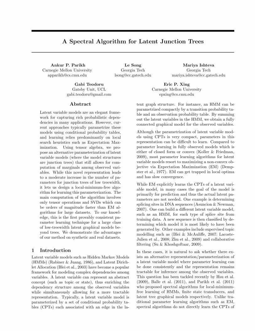
Figure 1: Our algorithm for local-minimum-free learning of latent variable models consist of four major steps. (1) First,we transform a model into a junction tree, such that each node in the junction tree corresponds to a maximal cliqueof variables in the triangulated graph of the original model. (2) Then we embed the clique potentials of the junctiontree into higher order tensors and express the marginal distribution of the observed variables as a tensor-tensor/matrixmultiplication according to the message passing algorithm. (3) Next we transform the tensor representation by insertinga pair of transformations between those tensor-tensor/matrix operations. Each pair of transformations is chosen so thatthey are inversions of each other. (4) Lastly, we show that each transformed representation is a function of only observedvariables. Thus, we can estimate each individual transformed tensor quantity using samples from observed variables.
a latent variable model. Instead they learn an alter-native parameterization (called the observable repre-sentation) which generally contains a larger numberof parameters than the CPTs, but where computingobserved marginals is still tractable. Moreover, thesealternative parameters have the advantage that theyonly depend on observed variables and can thereforebe directly estimated from data. Thus, parameterlearning in the alternative representation is fast, local-minimum-free, and provably consistent. Furthermore,spectral algorithms can be generalized to nonparamet-ric latent models (Song et al., 2010, 2011) where it isdifficult to run EM.
However, existing spectral algorithms apply onlyto restricted latent structures (HMMs and latenttrees), while latent structures beyond trees, such ashigher order HMMs (Kundu et al., 1989), factorialHMMs (Ghahramani & Jordan, 1997) and DynamicBayesian Networks (Murphy, 2002), are needed andhave been proven useful in many real world prob-lems. The challenges for generalizing spectral algo-rithms to general latent structured models include thelarger factors, more complicated conditional indepen-dence structures, and the need to sum out multiplevariables simultaneously.
The goal of this paper is to develop a new represen-tation for latent variable models with structures be-yond trees, and design a spectral algorithm for learningthis representation. We will focus on latent junctiontrees; thus the algorithm is suitable for both directedand undirected models which can be transformed intojunction trees. Concurrently to our work, Cohen et al.(2012) proposed a spectral algorithm for Latent Prob-abilistic Context Free Grammars (PCFGs). LatentPCFGs are not trees, but have many tree-like prop-erties, and so the representation Cohen et al. (2012)propose does not easily extend to other non-tree mod-els such as higher order/factorial HMMs that we con-sider here. Our more general approach requires more
complex tensor operations, such as multi-mode inver-sion, that are not used in the latent PCFG case.
The key idea of our approach is to embed the cliquepotentials of the junction tree into higher order tensorssuch that the computation of the marginal probabil-ity of observed variables can be carried out via tensoroperations. While this novel representation leads onlyto a moderate increase in the number parameters forjunction trees of low treewidth, it allows us to designan algorithm that can recover a transformed version ofthe tensor parameterization and ensure that the jointprobability of observed variables are computed cor-rectly and consistently. The main computation of thealgorithm involves only tensor operations and singu-lar value decompositions (hence the name “spectral”)which can be orders of magnitude faster than EM al-gorithms in large datasets. To our knowledge, this isthe first provably consistent parameter learning tech-nique for a large class of low-treewidth latent graph-ical models beyond trees. In our experiments withlarge scale synthetic datasets, we show that our spec-tral algorithm can be almost 2 orders of magnitudefaster than EM while at the same achieving consid-erably better accuracy. Our spectral algorithm alsoachieves comparable accuracy to EM on real data.
Organization of paper. A high level overview ofour approach is given in Figure 1. We first providesome background on tensor algebra and latent junc-tion trees. We then derive the spectral algorithm byrepresenting junction tree message passing with ten-sor operations, and then transform this representationinto one that only depends on observed variables. Fi-nally, we analyze the sample complexity of our methodand evaluate it on synthetic and real datasets.
2 Tensor Notation
We first give an introduction to the tensor nota-tion tailored to this paper. An Nth order tensor isa multiway array with N “modes”, i.e., N indices

{i1, i2, . . . , iN} are needed to access its entries. Sub-arrays of a tensor are formed when a subset of theindices is fixed, and we use a colon to denote allelements of a mode. For instance, A(i1, . . . , in−1, :, in+1, . . . , iN ) are all elements in the nth modeof a tensor A with indices from the other N −1 modes fixed to {i1, . . . , in−1, in+1, . . . , iN} respec-tively. Furthermore, we also use the shorthand ip:q ={ip, ip+1, . . . , iq−1, iq} for consecutive indices, e.g.,A(i1, . . . , in−1, :, in+1, . . . , iN ) = A(i1:n−1, :, in+1:N ).
Labeling tensor modes with variables. In con-trast to the conventional tensor notation such as theone described in Kolda & Bader (2009), the ordering ofthe modes of a tensors will not be essential in this pa-per. We will use random variables to label the modesof a tensor: each mode will correspond to a randomvariable and what is important is to keep track of thiscorrespondence. Therefore, we think two tensors areequivalent if they have the same set of labels and theycan be obtained from each other by a permutation ofthe modes for which the labels are aligned.
In the matrix case this translates to A and A> beingequivalent in the sense that A> carries the same in-formation as A, as long as we remember that the rowsof A> are the columns of A and vice versa. We willuse the following notation to denote this equivalence
A ∼= A> (1)
Under this notation, the dimension (or the size) of amode labeled by variable X will be the same as thenumber of possible values for variableX. Furthermore,when we multiply two tensors together, we will alwayscarry out the operation along (a set of) modes withmatching labels.
Tensor multiplication with mode labels. LetA ∈ RI1×I2×···×IN be an Nth order tensor and B ∈RJ1×J2×···×JM be an Mth order tensor. If X is a com-mon mode label for both A and B (w.l.o.g. we assumethat this is the first mode, implying also that I1 = J1),multiplying along this mode will give
C = A×X B ∈ RI2×···×IN×J2×···×JM , (2)
where the entries of C is defined as
C(i2:N , j2:M ) =∑I1
i=1A(i, i2:N )B(i, j2:M )
Similarly, we can multiply two tensors along multiplemodes. Let σ = {X1, . . . , Xk} be an arbitrary set ofk modes (k variables) shared by A and B (w.l.o.g. weassume these labels correspond to the first k modes,and I1 = J1, . . . , Ik = Jk holds for the correspond-ing dimensions). Then multiplying A and B along σresults in
D = A×σ B ∈ RIk+1×...×IN×Jk+1×...×JM , (3)
where the entries of D are defined as
D(ik+1:N , jk+1:M ) =∑i1:k
A(i1:k, ik+1:N )B(i1:k, jk+1:M ).
Multi-mode multiplication can also be interpreted asreshaping the σ modes of A and B into a single modeand doing single-mode tensor multiplication. Further-more, tensor multiplication with labels is symmetricin its arguments, i.e., A×σ B ∼= B ×σ A.
Mode-specific identity tensor. We now define ournotion of identity tensor with respect to a set of modesσ = {X1, . . . , XK}. Let A be a tensor with mode la-bels containing σ, and Iσ be a tensor with 2K modeswith mode labels {X1, . . . , XK , X1, . . . , XK}. ThenIσ is an identity tensor with respect to modes σ if
A×σ Iσ ∼= A. (4)
One can also understand Iσ using its matrix repre-sentation: flattening Iσ with respect to σ (the firstσ modes mapped to rows and the second σ modesmapped to columns) results in an identity matrix.
Mode-specific tensor inversion. Let F ,F−1 ∈RI1×···×IK×IK+1×···×IK+K′ be tensors of order K +K ′, and both have two sets of mode labels σ ={X1, . . . , XK} and ω′ = {XK+1, . . . , XK+K′}. ThenF−1 is the inverse of F w.r.t. modes ω if and only if
F ×ω F−1 ∼= Iσ. (5)
Multimode inversion can also be interpreted as re-shaping F with respect to ω into a matrix of size(I1 . . . IK)× (IK+1 . . . IK+K′), taking the inverse, andthen rearranging back into a tensor. Thus the exis-tence and uniqueness of this inverse can be character-ized by the rank of the matricized version of F .
Mode-specific diagonal tensors. We use δ todenote an N -way relation: its entry δ(i1:N ) at po-sition i1:N equals 1 when all indexes are the same(i1 = i2 = . . . = iN ), and 0 otherwise. We willuse �d to denote repetition of an index d times. Forinstance, we use P(�dX) to denote a dth order ten-sor where its entries at (i1:d)th position are specifiedby δ(i1:d)P(X = xi1). A diagonal matrix with itsdiagonal equal to P(X) is then denoted as P(�2X).Similarly, we can define a (d + d′)th order tensorP(�dX|�d′Y ) where its (i1:dj1:d′)th entry correspondsto δ(i1:d)δ(j1:d′)P(X = xi1 |Y = yj1).
3 Latent Junction Trees
In this paper, we will focus on discrete latent vari-able models where the number of states, kh, for eachhidden variable is much smaller than the number ofstates, ko, for each observed variable. Uppercase let-ters denote random variables (e.g., Xi) and lowercaseletters their instantiations (e.g., xi). A latent variablemodel defines a joint probability distribution over aset of variables X = O ∪H . Here, O denotes the setof observed variables,
{X1, . . . , X|O|
}. H denotes the
set of hidden variables,{X|O|+1, . . . , X|H |+|O|
}.
We will focus on latent variable models where the

structure of the model is a junction tree of lowtreewidth (Cowell et al., 1999). Each node Ci ina junction tree corresponds to a subset (clique) ofvariables from the original graphical model. We willalso use Ci to denote the collection of variables con-tained in the node, i.e. Ci ⊂ X . Let C denote theset of all clique nodes. The treewidth is then thesize of a largest clique in a junction tree minus one,that is t = maxCi∈C |Ci| − 1. Furthermore, we asso-ciate each edge in a junction tree with a separator setSij := Ci ∩ Cj which contains the common variablesof the two cliques Ci and Cj it is connected to. If wecondition on all variables in any Sij , the variables ondifferent sides of Sij will become independent.
Without loss of generality, we assume that each in-ternal clique node in the junction tree has exactly 3neighbors.1 Then we can pick a clique Cr as the rootof the tree and reorient all edges away from the rootto induce a topological ordering of the clique nodes.Given the ordering, the root node will have 3 childrennodes, denoted as Cr1 , Cr2 and Cr3 . Each other inter-nal node Ci will have a unique parent node, denotedas Ci0 , and 2 children nodes denoted as Ci1 and Ci2 .Each leaf node Cl is only connected with its uniqueparent node Cl0 . Furthermore, we can simplify thenotation for the separator set between a node Ci andits parent Ci0 as Si = Ci ∩Ci0 , omitting the index forthe parent node. Then the remainder set of a nodeis defined as Ri = Ci \ Si. We also assume w.l.o.g.that if Ci is a leaf in the junction tree, Ri consists ofonly observed variables. We will use ri to denote aninstantiation of the set of variables in Ri. See Figure 2for an illustration of notation.
Given a root and a topological ordering of the nodesin a junction tree, the joint distribution of all variablesX can be factorized according to
P(X ) =∏|X |
i=1P(Ri|Si), (6)
where each CPT P(Ri|Si), also called a clique poten-tial, corresponds to a node Ci. The number of param-eters needed to specify the model is O(|C|kto), linearin the number of cliques but exponential in the treewidth t. Then the marginal distribution of the ob-served variables can be obtained by summing over thelatent variables,
P(O) =∑
X|O|+1
. . .∑
X|O|+|H |
|X |∏i=1
P(Ri|Si)
, (7)
where we use∑X φ(X) to denote summation over all
possible instantiations of φ(x) w.r.t. variable X. Notethat each (non-leaf) remainder set Ri contains a smallsubset of all latent variables. The presence of latent
1If this is not the case, the derivation is similar butnotationally much heavier.
𝐶𝑖1 𝐶𝑖2
𝐶𝑖
𝐶𝑖0
𝑆𝑖1 𝑆𝑖2
𝑆𝑖
𝑆𝑖0
𝑅𝑖 = 𝐶𝑖 ∖ 𝑆𝑖
𝐴
𝐵
𝐶 𝐷
𝐸
𝐺
𝐻
𝐼
𝐹 𝐵𝐶𝐹 𝐵𝐷𝐺
𝐵𝐶𝐷𝐸
𝐴𝐶𝐸
𝐵𝐶 𝐵𝐷
𝐶𝐸
𝐴𝐶𝐻 𝐶𝑗
𝐺 ∈ 𝒪𝑖1
𝐹 ∈ 𝒪𝑖2
𝐹, 𝐺 ∈ 𝒪𝑖
𝐻 ∈ 𝒪𝑖−
Figure 2: Example latent variable models with variablesX = {A,B,C,D,E, F,G,H, I, . . .}, the observed variablesare O = {F,G,H, . . .} (only partially drawn). Its corre-sponding junction tree is shown in the middle panel. Cor-responding to this junction tree, we also show the generalnotation for it in the rightmost panel.
variables introduces complicated dependency betweenobserved variables, while at the same time only a smallnumber of parameters corresponding to the entries inthe CPTs are needed to specify the model.
The process of eliminating the latent variables in (7)can be carried out efficiently via message passing.More specifically, the summation can be broken up intolocal computation for each node in the junction tree.Each node only needs to sum out a small number ofvariables and then the intermediate result, called themessage, is passed to its parent for further process-ing. In the end the root node incorporates all messagesfrom its children and produces the final result P (O).The local summation step, called the message update,can be generically written as2
M(Si) =∑
Ri
P(Ri|Si)M(Si1)M(Si2) (8)
where we use M(Si) to denote the intermediate re-sults of eliminating variables in the remainder set Ri.This message update is then carried out recursivelyaccording the reverse topological order of the junctiontree until we reach the root node. The local sum-mation step for the leaf nodes and root node can beviewed as special cases of (8). For a leaf node Cl,there is no incoming message from children nodes,and hence M(Sl) = P(rl|Sl); for the root node Cr,Sr = ∅ and Ri = Ci, and hence P(O) = M(∅) =∑∀X∈Cr
P(Cr)M(Sr1)M(Sr2)M(Sr3).
Example. The message update at the internal nodeCBCDE in Figure 2 is
M({C,E}) =∑
B,DP(B,D|C,E)P(f |B,C)P(g|B,D).
4 Tensor Representation for MessagePassing
Although the parametrization of latent junction treesusing CPTs is very compact and inference (messagepassing) can be carried out efficiently, parameters inthis representation can be difficult to learn. Since thelikelihood of the observed data is no longer convex inthe latent parameters, local search heuristics, such as
2For simplicity of notation, assume Ci = Si ∪ Si1 ∪ Si2 .

EM, are often employed to learning the parameters.Therefore, our goal is to design a new representationfor latent junction trees, such that subsequent learningcan be carried out in a local-minimum-free fashion.
In this section, we will develop a new representationfor the message update in (8) by embedding each CPTP(Ri|Si) into a higher order tensor P(Ci) . As we willsee, there will be two advantages to the tensor form.The first is that tensor multiplication can be used tocompactly express the sum and product steps involvedin message passing. As a very simplistic example, letPA|B = P(A|B) be a conditional probability matrixand PB = P(B) be a marginal probability vector.Then matrix-vector multiplication, PA|BPB = P (A),sums out variable B. However, if we put the marginalprobability of B on the diagonal of a matrix, then Bwill not be summed out: e.g., if P�2B = P(�2B), thenPA|BP�2B = P(A,B) (but now B is no longer on thediagonal). We will leverage these facts to derive ourtensor representation for message passing.
Moreover, we can then utilize tensor inversion to con-struct an alternate parameterization. In the verysimplistic (matrix) example, note that P(A,B) =PA|BP�2B = PA|BFF
−1P�2B . The invertible trans-formations F will give us an extra degree of freedomto allow us to design an alternate parameterization ofthe latent junction tree that is only a function of ob-served variables. This would not be possible in thetraditional representation (Eq. 8).
4.1 Embed CPTs to higher order tensors
As we can see from (6), the joint probability distri-bution of all variables can be represented by a setof conditional distributions over just subsets of vari-ables. Each one of this conditionals is a low ordertensor. For example in Figure 2, the CPT correspond-ing to the clique node CBCDE would be a 4th ordertensor P(B,D|C,E) where each variable correspondsto a different mode of the tensor. However, this rep-resentation is not suitable for deriving the observablerepresentation since message passing cannot be definedeasily using the tensor multiplication/sum connectionshown above. Instead we will embed these tensors intoeven higher order tensors to facilitate the computation.The key idea is to introduce duplicate indexes usingthe mode-specific identity tensors, such that the sum-product steps in message updates can be expressed astensor multiplications.
More specifically, the number of times a mode of thetensor is duplicated will depend on how many timesthe corresponding variable in the clique Ci appears inthe separator sets incident to Ci. We can define thecount for a variable Xj ∈ Ci as
dj,i = I[Xj ∈ Si] + I[Xj ∈ Si1 ] + I[Xj ∈ Si2 ], (9)
where I[·] is an indicator function taking value 1 if itsargument is true and 0 otherwise. Then the tensorrepresentation of the node Ci is
P(Ci) :=P(. . . , (�dj,iXj), . . .︸ ︷︷ ︸
∀Xj∈Ri
| . . . , (�dj′,iXj′), . . .︸ ︷︷ ︸∀Xj′∈Si
), (10)
where the labels for the modes of the ten-sor are the combined labels of the separatorsets, i.e., {Si, Si1 , Si2}. The number of times a variableis repeated in the label set is exactly equal to dj,i.
Essentially, tensor P(Ci) contains exactly the sameinformation as the original CPT P(Ri|Si). Further-more, P(Ci) has a lot of zero entries, and the entriesfrom P(Ri|Si) are simply embedded in the higher or-der tensor P(Ci). Suppose all variables in node Ciare latent variables each taking kh values. Then the
number of entries needed to specify P(Ri|Si) is k|Ci|h ,
while the high order tensor P(Ci) has kdih entries where
di :=∑j:Xj∈Ci
dj,i which is never smaller than k|Ci|h .
In a sense, the parametrization using higher order ten-sor P(Ci) is less compact than the parametrizationusing the original CPTs. However, constructing thetensor P this way allows us to express the junctiontree message update step in (8) as tensor multipli-cations (more details in the next section), and thenwe can leverage tools from tensor analysis to design alocal-minimum-free learning algorithm.
The tensor representation for the leaf nodes andthe root node are special cases of the representationin (10). The tensor representation at a leaf nodeCl is simply equal to its CPT P(Cl) = P(Rl|Sl).The root node Cr has no parent, so P(Cr) =P(. . . , (�dj,rXj), . . .), ∀Xj ∈ Cr. Furthermore, sincedj,i is simply a count of how many times a variable inCi appears in each of the incident separators, the sizeof each tensor does not depend on which clique nodewas selected as the root.
Example. In Figure 2, node CBCDE corresponds toCPT P(B,D|C,E). Its high order tensor representa-tion is P(CBCDE) = P(�2B,D| �2 C,E), since bothB and C occur twice in the separator sets incident toCBCDE . Therefore the tensor P({B,C,D,E}) is a6th order tensor with mode labels {B,B,D,C,C,E}.
4.2 Tensor message passing
With the higher order tensor representation for cliquepotentials in the junction tree as in (10), we can ex-press the message update step in (8) as tensor multipli-cations. Consequently, we can compute the marginaldistribution of the observed variables O in equation (7)recursively using a sequence of tensor multiplications.More specifically the general message update equation
for a node in a junction tree can be expressed as
M(Si) = P(Ci)×Si1M(Si1)×Si2
M(Si2). (11)
Here the modes of the tensor P(Ci) are labeled by thevariables, and the mode labels are used to carry outtensor multiplications as explained in Section 2. Es-sentially, multiplication with respect to the duplicatedmodes of the tensor P(Ci) will implement some kindof element-wise multiplication for the incoming mes-sages and then summation over the variables in theremainder set Ri.
The tensor message passing steps in leaf nodes and theroot node are special cases of the tensor message up-date in equation (11). The outgoing message M(Sl)at a leaf node Cl can be computed by simply setting allvariables in Rl to the actual observed values rl, i.e.,
M(Sl) = P(Cl)Rl=rl = P(Rl = rl|Sl). (12)
In this step, there is no difference between the aug-mented tensor representation and the standard mes-sage passing in junction tree. At the root, we arriveat the final results of the message passing algorithm,and we obtain the marginal probability of the observedvariables by aggregating all incoming messages fromits 3 children, i.e.,
P(O) = (13)P(Cr)×Sr1
M(Sr1)×Sr2M(Sr2)×Sr3
M(Sr3).
Example. For Figure 2, using the following tensors
P({B,C,D,E}) = P(�2B,D | �2 C,E)M({B,C}) = P(f |B,C)M({B,D}) = P(g|B,D),
we can write the message update for node CBCDE inthe form of equation (11) as
M({C,E}) = P({B,C,D,E})×{B,C}M({B,C})×{B,D}M({B,D}).
Note how the tensor multiplication sums out B andD: P({B,C,D,E}) has two B labels, and it appearsin the subscripts of tensor multiplication twice; D ap-pears once in the label and in the subscript of ten-sor multiplication respectively. Similarly, C is notsummed out since there are two C labels but it appearsonly once in the subscript of tensor multiplication.
5 Transformed Representation
Explicitly learning the tensor representation in (10) isstill an intractable problem. Our key observation isthat we do not need to recover the tensor represen-tation explicitly if our focus is to perform inferenceusing the message passing algorithm as in (11)–(13).As long as we can recover the tensor representation upto some invertible transformation, we can still obtainthe correct marginal probability P(O).
More specifically, we can insert a mode-specific iden-tity tensor Iσ into the message update equationin (11) without changing the outgoing message. Sub-
sequently, we can then replace the mode-specific iden-tity tensor by a pair of tensors, F and F−1, which aremode-specific inversions of each other (F ×ω F−1 ∼=Iσ). Then we can group these inserted tensors withthe representation P(C) from (10), and obtain a trans-
formed version P(C) (also see Figure 1). Furthermore,we have the freedom in choosing these collections oftensor inversion pairs. We will show that if we choosethem systematically, we will be able to estimate eachtransformed tensor P(C) using the marginal proba-bility of a small set of observed variables (observablerepresentation). In this section, we will first explainthe transformed tensor representation.
As an illustration, consider a sequence of matrix mul-tiplications with two identity matrices I1 = F1F
−11
and I2 = F2F−12 inserted
ABC = A(F1F−11 )B(F2F
−12 )C
= (AF1)︸ ︷︷ ︸A
(F−11 BF2)︸ ︷︷ ︸B
(F−12 C)︸ ︷︷ ︸C
.
We see that we can equivalently compute ABC usingtheir transformed versions, i.e., ABC = ABC.
Moving to the tensor case, let us first consider a nodeCi and its parent node Ci0 . Then the outgoing messageof Ci0 can be computed recursively as
M(Si0) = P(Ci0)×SiM(Si)︸ ︷︷ ︸
P(Ci)×Si1M(Si1 )×Si2
M(Si2 )
× . . .
Inserting a mode specific identity tensor ISiwith la-
bels {Si, Si} and similarly defined mode specific iden-tity tensors ISi1
and ISi2into the above two message
updates, we obtain
M(Si0) = P(Ci0)×Si (ISi ×Si M(Si)︸ ︷︷ ︸P(Ci)×Si1
(ISi1×Si1
M(Si1 ))×Si2(ISi2
×Si2M(Si1
))
)× . . .
Then we can further expand ISi using tensor inver-sion pairs F i, F−1i , i.e., ISi = F i ×ωi F
−1i . Note
that both F and F−1 have two set of mode labels,Si and another set ωi which is related to the observ-able representation and explained in the next section.Similarly, we expand ISi1
and ISi2using their corre-
sponding tensor inversion pairs.
After expanding tensor identities I, we can regroupterms, and at node Ci we have
M(Si) =(P(Ci)×Si1F i1 ×Si2
F i2) (14)
×ωi1(F−1i1 ×Si1
M(Si1))
×ωi2(F−1i2 ×Si2
M(Si2))
and at the parent node Ci0 of Ci
M(Si0) =(P(Ci0)×Si F i × . . .) (15)
×ωi(F−1i ×Si
M(Si))× . . .Now we can define the transformed tensor representa-tion for P(Ci) as
P(Ci) := P(Ci)×Si1F i1 ×Si2
F i2 ×Si F−1i , (16)
where the two transformations F i1 and F i2 are ob-
tained from the children side and the transformationF−1i is obtained from the parent side. Similarly, wecan define the transformed representation for a leafnode and for the root node as
P(Cl) = P(Cl)×SlF−1l (17)
P(Cr) = P(Cr)×Sr1Fr1 ×Sr2
Fr2 ×Sr3Fr3 (18)
Applying these definitions of the transformed repre-sentation recursively, we can perform message passingbased purely on these transformed representations
M(Si0) = P(Ci0)×ωi M(Si)︸ ︷︷ ︸P(Ci)×ωi1
M(Si1)×ωi2
M(Si2)
× . . . (19)
6 Observable Representation
In the transformed tensor representation in (16)-(18),we have the freedom of choosing the collection of ten-sor pairs F and F−1. We will show that if we choosethem systematically, we can recover each transformedtensor P(C) using the marginal probability of a smallset of observed variables (observable representation).
We will focus on the transformed tensor representa-tion in (16) for an internal node Ci (other cases fol-low as special cases). Due to the recursive way thetransformed representation is defined, we only havethe freedom of choosing F i1 and F i2 in this formula;the choice of F i will be fixed by the parent node ofCi. The idea is to choose
• F i1 = P(Oi1 |Si1) as the conditional distributionof some set of observed variables Oi1 ⊂ O in thesubtree rooted at child node Ci1 of node Ci, con-ditioning on the corresponding separator set Si1 .
• Similarly, we choose F i2 = P(Oi2 |Si2) whereOi2 ⊂ O and it lies in subtree rooted at Ci2 .
• Following this convention, F i is chosen by theparent node Ci0 and is fixed to P(Oi|Si).
Therefore, we have
P(Ci) = P(Ci)×Si1P(Oi1 |Si1)×Si2
P(Oi2 |Si2)
×Si P(Oi|Si)−1, (20)
where the first two tensor multiplications essentiallyeliminate the latent variables in Si1 and Si2 .3 Withthese choices, we also fix the mode labels ωi, ωi1 andωi2 in (14) (15) and (19). That is ωi = Oi, ωi1 = Oi1and ωi2 = Oi2 .
To remove all dependencies on latent variables inP(Ci) and relate it to observed variables, we needto eliminate the latent variables in Si and the ten-sor P(Oi|Si)−1. For this, we multiply the transformed
tensor P(Ci) by P(Oi,Oi−), where Oi− denotes someset of observed variables which do not belong to thesubtree rooted at node Ci. Furthermore, P(Oi,Oi−)can be re-expressed using the conditional distribution
3If a latent variable in Si1 ∪ Si2 is also in Si, it is noteliminated in this step but in another step.
of Oi and Oi− respectively, conditioning on the sepa-rator set Si, i.e.,
P(Oi,Oi−) = P(Oi|Si)×Si P(�2Si)×Si P(Oi−|Si).Therefore, we have
P(Oi|Si)−1 ×Oi P(Oi,Oi−) = P(�2Si)×Si P(Oi−|Si),and plugging this into (20), we have
P(Ci)×OiP(Oi,Oi−)
=P(Ci)×Si1P(Oi1 |Si1)×Si2
P(Oi2 |Si2)
×SiP(�2Si)×Si
P(Oi−|Si)=P(Oi1 ,Oi2 ,Oi−), (21)
where P(Ci) is now related to only marginal prob-abilities of observed variables. From the equivalentrelation, we can inverting P(Oi,Oi−), and obtain the
observable representation for P(Ci)
P(Ci) = P(Oi1 ,Oi2 ,Oi−)×Oi− P(Oi,Oi−)−1. (22)
Example. For node CBCDE in Figure 2, the choicesof Oi,Oi1 ,Oi2 and Oi− are {F,G}, G, F and H re-spectively.
There are many valid choices of Oi−. In the supple-mentary, we describe how these different choices canbe combined via a linear system using Eq. 21. Thiscan substantially increase performance.
For the leaf nodes and the root node, the derivationfor their observable representations can be viewed asspecial cases of that for the internal nodes. We providethe results for their observable representation below:
P(Cr) = P(Or1 ,Or2 ,Or3), (23)
P(Cl) = P(Ol,Ol−)×Ol− P(Ol,Ol−)−1. (24)
If P(Ol,Ol−) is invertible, then P(Cl) = IOl. Oth-
erwise we need to project P(Oi,Oi−) using a tensorU i to make it invertible, as discussed in the next sec-tion. The overall algorithm is given in Algorithm 1.Given N i.i.d. samples of the observed nodes, we sim-ply replace P(·) by the empirical estimate P(·).
Algorithm 1 Spectral algorithm for latent junction tree
In: Junction tree topology and N i.i.d. samples{xs1, . . . , x
s|O|}Ns=1
Out: Estimated marginal P(O)1: Estimate P(Ci) for the root, leaf and internal nodes
P(Cr) = P(Or1 ,Or2 ,Or3)×Or1Ur1 ×Or2
Ur2 ×Or3Ur3
P(Cl) = P(Ol,Ol−)×Ol− (P(Ol,Ol−)×OlU l)−1
P(Ci) = P(Oi1 ,Oi2 ,Oi−)×Oi1U i1 ×Oi2
U i2
×Oi− (P(Oi,Oi−)×Oi U i)−1
2: In reverse topological order, leaf and internal nodessend messages
M(Sl) = P(Cl)Ol=ol
M(Si) = P(Ci)×Oi1M(Si1)×Oi2
M(Si2)
3: At the root, obtain P(O) by
P(Cr)×Or1M(Sr1)×Or2
M(Sr2)×Or3M(Sr3)

7 Discussion
The observable representation exists only if there existtensor inversion pairs F i = P(Oi|Si), and F−1i . Thisis equivalent to requiring that the rank of the matri-cized version of F i (rows corresponds to modes Oi andcolumn to modes Si) has rank τi := kh×|Si|. Similarly.the matricized version of P(O−i|Si) also needs to haverank τi, so that the matricized version of P(Oi,Oi−)has rank τi and is invertible. Thus, it is required that#states(Oi) ≥ #states(Si). This can be achieved byeither making Oi consist of a few high dimensional ob-servations, or of many smaller dimensional ones. Inthe case when #states(Oi) > #states(Si), we need toproject F i to a lower dimensional space using a ten-sor U i so that it can be inverted. In this case, wedefine F i := P(Oi|Si) ×Oi
U i. For example, follow-ing this through the computation for the leaf gives usthat P(Cl) = P(Ol,Ol−)×Ol− (P(Ol,Ol−)×Ol
U l)−1.
A good choice of U i can be obtained by performing asingular value decomposition of the matricized versionof P(Oi,Oi−) (variables in Oi are arranged to rows andthose in Oi− to columns).
For HMMs and latent trees, this rank condition canbe expressed simply as requiring the conditional prob-ability tables of the underlying model to not be rank-deficient. However, junction trees encode more com-plex latent structures that introduce subtle considera-tions. A general characterization of the existence con-dition for observable representation with respect tothe graph topology will be our future work. In theappendix, we give some intuition using a couple of ex-amples where observable representations do not exist.
8 Sample Complexity
We analyze the sample complexity of Algorithm 1 andshow that it depends on the junction tree topologyand the spectral properties of the true model. Let dibe the order of P(Ci) and ei be the number of modesof P(Ci) that correspond to observed variables.
Theorem 1 Let τi = kh × |Si|, dmax = maxi di, andemax = maxi ei. Then, for any ε > 0, 0 < δ < 1, if
N ≥ O
((4k2h3β2
)dmax kemaxo ln |C|δ |C|
2
ε2α4
)where στ (∗) returns the τ th largest singular value and
α = mini στi(P(Oi,O−i)), β = mini στi(F i)
Then with probability 1− δ,∑x1,...,x|O|
∣∣∣P(x1, . . . , x|O|)− P(x1, . . . , x|O|)∣∣∣ ≤ ε .
See the supplementary for a proof. The result impliesthat the estimation problem depends exponentially ondmax and emax, but note that emax ≤ dmax. Fur-thermore, dmax is always greater than or equal to thetreewidth. Note the dependence on the singular val-ues of certain probability tensors. In fully observed
models, the accuracy of the learned parameters de-pends only on how close the empirical estimates of thefactors are to the true factors. However, our spec-tral algorithm also depends on how close the inversesof these empirical estimates are to the true inverses,which depends on the spectral properties of the matri-ces (Stewart & Sun, 1990).
9 Experiments
We now evaluate our method on synthetic and realdata and compare it with both standard EM (Demp-ster et al., 1977) and stepwise online EM (Liang &Klein, 2009). All methods were implemented in C++,and the matrix library Eigen (Guennebaud et al.,2010) was used for computing SVDs and solving linearsystems. For all experiments, standard EM is given 5random restarts. Online EM tends to be sensitive tothe learning rate, so it is given one restart for eachof 5 choices of the learning rate {0.6, 0.7, 0.8, 0.9, 1}(the one with highest likelihood is selected). Conver-gence is determined by measuring the change in thelog likelihood at iteration t (denoted by f(t)) over the
average: |f(t)−f(t−1)|avg(f(t),f(t−1)) ≤ 10−4 (the same precision as
used in Murphy (2005)).
For large sample sizes our method is almost two or-ders of magnitude faster than both EM and onlineEM. This is because EM is iterative and every iter-ation requires inference over all the training exampleswhich can become expensive. On the other hand, thecomputational cost of our method is dominated by theSVD/linear system. Thus, it is primarily dependentonly on the number of observed states and maximumtensor order, and can easily scale to larger sample sizes.
In terms of accuracy, we generally observe 3 distinctregions, low-sample size, mid-sample size, and largesample size. In the low sample size region, EM/onlineEM tend to overfit to the training data and our spec-tral algorithm usually performs better. In the mid-sample size region EM/online EM tend to perform bet-ter since they benefit from a smaller number of param-eters. However, once a certain sample size is reached(the large sample size region), our spectral algorithmconsistently outperforms EM/online EM which sufferfrom local minima and convergence issues.
9.1 Synthetic Evaluation
We first perform a synthetic evaluation. 4 different la-tent structures are used (see Figure 3): a second ordernonhomogenous (NH) HMM, a third order NH HMM,a 2 level NH factorial HMM, and a complicated syn-thetic junction tree. The second/third order HMMshave kh = 2 and ko = 4, while the factorial HMM andsynthetic junction tree have kh = 2, and ko = 16. Foreach latent structure, we generate 10 sets of model pa-rameters, and then sample N training points and 1000

test points from each set, whereN is varied from 100 to100, 000. For evaluation, we measure the accuracy of
joint estimation using error = |P(x1,...,xO)−P(x1,...,xO)|P(x1,...,xO) .
We also measure the training time of both methods.
Figure 3 shows the results. As discussed earlier, ouralgorithm is between one and two orders of magnitudefaster than both EM and online EM for all the latentstructures. EM is actually slower for very small samplesizes than for mid-range sample sizes because of over-fitting. Also, in all cases, the spectral algorithm hasthe lowest error for large sample sizes. Moreover, criti-cal sample size at which spectral overtakes EM/onlineEM is largely dependent on the number of parametersin the observable representation compared to that inthe original parameterization of the model. In higherorder/factorial HMM models, this increase is small,while in the synthetic junction tree it is larger.
9.2 Splice dataset
We next consider the task of determining splicing sitesin DNA sequences (Asuncion & Newman, 2007). Eachexample consists of a DNA sequence of length 60,where each position in the sequence is either an A, T ,C, or G. The goal is to classify whether the sequenceis an Intron/Exon site, Exon/Intron site, or neither.During training, for each class a different second or-der nonhomogeneous HMM with kh = 2 and ko = 4 istrained. At test, the probability of the test sequence iscomputed for each model, and the one with the high-est probability is selected (which we found to performbetter than a homogeneous one).
Figure 4, shows our results, which are consistent withour synthetic evaluation. Spectral performs the bestin low sample sizes, while EM/online EM perform alittle better in the mid-sample size range. The datasetis not large enough to explore the large sample sizeregime. Moreover, we note that spectral algorithm ismuch faster for all the sample sizes.
10 Conclusion
We have developed an alternative parameterizationthat allows fast, local minima free, and consistent pa-rameter learning of latent junction trees. Our ap-proach generalizes spectral algorithms to a much widerrange of structures such as higher order, factorial, andsemi-hidden Markov models. Unlike traditional non-convex optimization formulations, spectral algorithmsallow us to theoretically explore latent variable mod-els in more depth. The spectral algorithm depends notonly on the junction tree topology but also on the spec-tral properties of the parameters. Thus, two modelswith the same structure may pose different degrees ofdifficulty based on the underlying singular values. Thisis very different from learning fully observed junctiontrees, which is primarily dependent on only the topol-
...
Length = 40
...
Length = 40
0.1 0.2 0.5 1 2 5 10 20 50 75 100
0.1
0.2
0.30.40.5
1
2nd Order NonHomogeneous HMM
Training Sample Size (x103)
Err
or
Spectral
online−EM
EM
0.1 0.2 0.5 1 2 5 10 20 50 75 100
0.2
0.3
0.40.5
1
3rd Order NonHomogeneous HMM
Training Sample Size (x103)
Err
or
Spectral
online−EM
EM
0.1 0.2 0.5 1 2 5 10 20 50 75 100
10
100
1000
2nd Order NonHomogeneous HMM
Training Sample Size (x103)
Run
time
(s)
online−EM
EM
Spectral
0.1 0.2 0.5 1 2 5 10 20 50 75 100
100
1000
10000
3rd Order NonHomogeneous HMM
Training Sample Size (x103)
Run
time
(s) online−EM
EM
Spectral
(a) 2nd Order HMM (b) 3rd Order HMM
...
...
Length = 15
0.1 0.2 0.5 1 2 5 10 20 50 75 1000.2
0.3
0.40.5
1
2 Level Factorial HMM
Training Sample Size (x103)
Err
or
Spectral
online−EM
EM
0.1 0.2 0.5 1 2 5 10 20 50 75 100
0.1
0.2
0.30.40.5
1
Synthetic Junction Tree
Training Sample Size (x103)
Err
or Spectral
online−EM
EM
0.1 0.2 0.5 1 2 5 10 20 50 75 100
10
100
1000
100002 Level Factorial HMM
Training Sample Size (x103)
Run
time
(s)
Spectral
EM
online−EM
0.1 0.2 0.5 1 2 5 10 20 50 75 1001
10
100
1000
10000
Synthetic Junction Tree
Training Sample Size (x103)
Run
time
(s)
EM
online−EM
Spectral
(c) 2 Level Factorial HMM (d) Synthetic Junction Tree
Figure 3: Comparison of our spectral algorithm (blue) toEM (red) and online EM (green) for various latent struc-tures. Both errors and runtimes in log scale.
0.1 0.2 0.5 1 2 2.675
0.1
0.2
0.3
0.4
Splice
Training Sample Size (x103)
Err
or
Spectral
online−EM
EM
0.1 0.2 0.5 1 2 2.675
100
1000
Splice
Training Sample Size (x103)
Run
time
(s)
online−EM
EM
Spectral
Figure 4: Results on Splice dataset
ogy/treewidth. Future directions include learning dis-criminative models and structure learning.
Acknowledgements: This work is supported by anNSF Graduate Fellowship (Grant No. 0750271) toAPP, Georgia Tech Startup Funding to LS, NIH 1R01-GM093156, and The Gatsby Charitable Foundation.We thank Byron Boots for valuable discussion.

References
Asuncion, A. and Newman, D.J. UCI machine learningrepository, 2007.
Balle, B., Quattoni, A., and Carreras, X. A spec-tral learning algorithm for finite state transduc-ers. Machine Learning and Knowledge Discovery inDatabases, pp. 156–171, 2011.
Blei, David and McAuliffe, Jon. Supervised topic mod-els. In Advances in Neural Information ProcessingSystems 20, pp. 121–128. 2007.
Blei, D.M., Ng, A.Y., and Jordan, M.I. Latent dirich-let allocation. The Journal of Machine Learning Re-search, 3:993–1022, 2003.
Cohen, S.B., Stratos, K., Collins, M., Foster, D.P., andUngar, L. Spectral learning of latent-variable pcfgs.In Association of Computational Linguistics (ACL),volume 50, 2012.
Cowell, R., Dawid, A., Lauritzen, S., and Spiegelhal-ter, D. Probabilistic Networks and Expert Sytems.Springer, New York, 1999.
Dempster, A., Laird, N., and Rubin, D. Maximumlikelihood from incomplete data via the EM algo-rithm. Journal of the Royal Statistical Society B, 39(1):1–22, 1977.
Ghahramani, Z. and Jordan, M.I. Factorial hiddenMarkov models. Machine learning, 29(2):245–273,1997.
Guennebaud, G., Jacob, B., et al. Eigen v3.http://eigen.tuxfamily.org, 2010.
Hsu, D., Kakade, S., and Zhang, T. A spectral al-gorithm for learning hidden Markov models. InProc. Annual Conf. Computational Learning The-ory, 2009.
Kolda, T. and Bader, B. Tensor decompositions andapplications. SIAM Review, 51(3):455–500, 2009.
Koller, D. and Friedman, N. Probabilistic graphicalmodels: principles and techniques. The MIT Press,2009.
Kundu, A., He, Y., and Bahl, P. Recognition of hand-written word: first and second order hidden Markovmodel based approach. Pattern recognition, 22(3):283–297, 1989.
Lacoste-Julien, S., Sha, F., and Jordan, M.I. Disclda:Discriminative learning for dimensionality reductionand classification. volume 21, pp. 897–904. 2008.
Liang, P. and Klein, D. Online em for unsupervisedmodels. In Proceedings of human language tech-nologies: The 2009 annual conference of the NorthAmerican chapter of the association for computa-tional linguistics, pp. 611–619. Association for Com-putational Linguistics, 2009.
Murphy, K. Hidden Markov model (HMM) toolbox formatlab http://www.cs.ubc.ca/murphyk/software/.2005.
Murphy, K.P. Dynamic bayesian networks: represen-tation, inference and learning. PhD thesis, Univer-sity of California, 2002.
Parikh, A.P., Song, L., and Xing, E.P. A spectral algo-rithm for latent tree graphical models. In Proceed-ings of the 28th International Conference on Ma-chine Learning, pp. 1065–1072. ACM, 2011.
Rabiner, L. R. and Juang, B. H. An introduction tohidden Markov models. IEEE ASSP Magazine, 3(1):4–16, 1986.
Song, L., Boots, B., Siddiqi, S., Gordon, G., andSmola, A. Hilbert space embeddings of hiddenMarkov models. In Proceedings of the 27th Inter-national Conference on Machine Learning, pp. 991–998. ACM, 2010.
Song, L., Parikh, A.P., and Xing, E.P. Kernel embed-dings of latent tree graphical models. In Advancesin Neural Information Processing Systems (NIPS),volume 24, pp. 2708–2716. 2011.
Stewart, GW and Sun, J. Matrix Perturbation Theory.Academic Press, 1990.
Su, X. and Khoshgoftaar, T.M. A survey of collab-orative filtering techniques. Advances in ArtificialIntelligence, 2009:4, 2009.
Zhu, J., Ahmed, A., and Xing, E.P. Medlda: maxi-mum margin supervised topic models for regressionand classification. In Proceedings of the 26th AnnualInternational Conference on Machine Learning, pp.1257–1264. ACM, 2009.