arX

iv:n

lin.C

D/0

4080

44 v

1 2

6 A

ug 2

004

Int. J. Bifurcation and Chaos 13, 3147-3233, (2003). Tutorial and Review paper.

TOWARD A THEORY OF CHAOS

A. SenguptaDepartment of Mechanical EngineeringIndian Institute of Technology. Kanpur

E-Mail: osegu@iitk.ac.in

ABSTRACT

This paper formulates a new approach to the study of chaos in discrete dynamical systems based onthe notions of inverse ill-posed problems, set-valued mappings, generalized and multivalued inverses,graphical convergence of a net of functions in an extended multifunction space (Sengupta and Ray,2000), and the topological theory of convergence. Order, chaos, and complexity are described as distinctcomponents of this unified mathematical structure that can be viewed as an application of the theory ofconvergence in topological spaces to increasingly nonlinear mappings, with the boundary between orderand complexity in the topology of graphical convergence being the region in Multi(X) that is susceptibleto chaos. The paper uses results from the discretized spectral approximation in neutron transport theory(Sengupta, 1988, 1995) and concludes that the numerically exact results obtained by this approximation ofthe Case singular eigenfunction solution is due to the graphical convergence of the Poisson and conjugatePoisson kernels to the Dirac delta and the principal value multifunctions respectively. In Multi(X), thecontinuous spectrum is shown to reduce to a point spectrum, and we introduce a notion of latent chaoticstates to interpret superposition over generalized eigenfunctions. Along with these latent states, spectraltheory of nonlinear operators is used to conclude that nature supports complexity to attain efficiently amultiplicity of states that otherwise would remain unavailable to it.

Keywords: chaos, complexity, ill-posed problems, graphical convergence, topology, multifunctions.

Prologue

1. Generally speaking, the analysis of chaos is extremely difficult. While a general definition for chaosapplicable to most cases of interest is still lacking, mathematicians agree that for the special case of iterationof transformations there are three common characteristics of chaos:

1. Sensitive dependence on initial conditions,

2. Mixing,

3. Dense periodic points.

Peitgen et al. (1992)

2. The study of chaos is a part of a larger program of study of so-called“strongly”nonlinear system. · · ·Linearity means that the rule that determines what a piece of a system is going to do next is not influenced bywhat it is doing now. More precisely this is intended in a differential or incremental sense: For a linear spring,the increase of its tension is proportional to the increment whereby it is stretched, with the ratio of theseincrements exactly independent of how much it has already been stretched. Such a spring can be stretchedarbitrarily far · · · . Accordingly no real spring is linear. The mathematics of linear objects is particularlyfelicitous. As it happens, linear objects enjoy an identical, simple geometry. The simplicity of this geometryalways allows a relatively easy mental image to capture the essence of a problem, with the technicality, growingwith the number of parts, basically a detail. The historical prejudice against nonlinear problems is that no sosimple nor universal geometry usually exists.

Mitchell Feigenbaum’s Foreword (pp 1-7) in Peitgen et al. (1992)

1

3. The objective of this symposium is to explore the impact of the emerging science of chaos on variousdisciplines and the broader implications for science and society. The characteristic of chaos is its universalityand ubiquity. At this meeting, for example, we have scholars representing mathematics, physics, biology,geophysics and geophysiology, astronomy, medicine, psychology, meteorology, engineering, computer science,economics and social sciences1. Having so many disciplines meeting together, of course, involves the risk thatwe might not always speak the same language, even if all of us have come to talk about“chaos”.

Opening address of Heitor Gurgulino de Souza, Rector United Nations University, Tokyode Souza (1997)

4. The predominant approach (of how the different fields of science relate to one other) is reductionist:Questions in physical chemistry can be understood in terms of atomic physics, cell biology in terms of howbiomolecules work · · · . We have the best of reasons for taking this reductionist approach: it works. Butshortfalls in reductionism are increasingly apparent (and) there is something to be gained from supplementingthe predominantly reductionist approach with an integrative agenda. This special section on complex systemsis an initial scan (where) we have taken a“complex system”to be one whose properties are not fully explainedby an understanding of its component parts. Each Viewpoint author2 was invited to define “complex” as itapplied to his or her discipline.

Gallagher and Appenzeller (1999)

5. One of the most striking aspects of physics is the simplicity of its laws. Maxwell’s equations,Schroedinger’s equations, and Hamilton mechanics can each be expressed in a few lines. · · · Everythingis simple and neat except, of course, the world. Every place we look outside the physics classroom we seean world of amazing complexity. · · · So why, if the laws are so simple, is the world so complicated? To uscomplexity means that we have structure with variations. Thus a living organism is complicated because ithas many different working parts, each formed by variations in the working out of the same genetic coding.Chaos is also found very frequently. In a chaotic world it is hard to predict which variation will arise in a givenplace and time. A complex world is interesting because it is highly structured. A chaotic world is interestingbecause we do not know what is coming next. Our world is both complex and chaotic. Nature can producecomplex structures even in simple situations and obey simple laws even in complex situations.

Goldenfeld and Kadanoff (1999)

6. Where chaos begins, classical science stops. For as long as the world has had physicists inquiringinto the laws of nature, it has suffered a special ignorance about disorder in the atmosphere, in the turbulentsea, in the fluctuations in the wildlife populations, in the oscillations of the heart and the brain. But in the1970s a few scientists began to find a way through disorder. They were mathematicians, physicists, biologists,chemists · · · (and) the insights that emerged led directly into the natural world: the shapes of clouds, thepaths of lightning, the microscopic intertwining of blood vessels, the galactic clustering of stars. · · · Chaosbreaks across the lines that separate scientific disciplines, (and) has become a shorthand name for a fastgrowing movement that is reshaping the fabric of the scientific establishment.

Gleick (1987)

7. order −→ complexity −→ chaos.

Waldrop (1992)

8. Our conclusions based on these examples seems simple: At present chaos is a philosophical term, nota rigorous mathematical term. It may be a subjective notion illustrating the present day limitations of thehuman intellect or it may describe an intrinsic property of nature such as the“randomness”of the sequence ofprime numbers. Moreover, chaos may be undecidable in the sense of Godel in that no matter what definitionis given for chaos, there is some example of chaos which cannot be proven to be chaotic from the definition.

1A partial listing of papers is as follows: Chaos and Politics: Application of nonlinear dynamics to socio-

political issues; Chaos in Society: Reflections on the impact of chaos theory on sociology; Chaos in neural networks;

The impact of chaos on mathematics; The impact of chaos on physics; The impact of chaos on economic theory;

The impact of chaos on engineering; The impact of chaos on biology; Dynamical disease: and The impact of

nonlinear dynamics and chaos on cardiology and medicine.2The eight Viewpoint articles are titled: Simple Lessons from Complexity; Complexity in Chemistry; Complex-

ity in Biological Signaling Systems; Complexity and the Nervous System; Complexity, Pattern, and Evolutionary

Trade-Offs in Animal Aggregation; Complexity in Natural Landform Patterns; Complexity and Climate and Com-

plexity and the Economy.

2

Brown and Chua (1996)

9. My personal feeling is that the definition of a “fractal” should be regarded in the same way as thebiologist regards the definition of “life”. There is no hard and fast definition, but just a list of propertiescharacteristic of a living thing · · · . Most living things have most of the characteristics on the list, thoughthere are living objects that are exceptions to each of them. In the same way, it seems best to regard a fractalas a set that has properties such as those listed below, rather than to look for a precise definition which willcertainly exclude some interesting cases.

Falconer (1990)

10. Dynamical systems are often said to exhibit chaos without a precise definition of what this means.

Robinson (1999)

1. Introduction

The purpose of this paper is to present an unified, self-contained mathematical structure andphysical understanding of the nature of chaos in a discrete dynamical system and to suggesta plausible explanation of why natural systems tend to be chaotic. The somewhat extensivequotations with which we begin above, bear testimony to both the increasingly significant —and perhaps all-pervasive — role of nonlinearity in the world today as also our imperfect state ofunderstanding of its manifestations. The list of papers at both the UN Conference (de Souza,1997) and in Science (Gallagher and Appenzeller, 1999) is noteworthy if only to justify theobservation of Gleick (1987) that “chaos seems to be everywhere”. Even as everybody appearsto be finding chaos and complexity in all likely and unlikely places, and possibly because of it, itis necessary that we have a clear mathematically-physical understanding of these notions thatare supposedly reshaping our view of nature. This paper is an attempt to contribute to this goal.To make this account essentially self-contained we include here, as far as this is practicable, thebasics of the background material needed to understand the paper in the form of Tutorials andan extended Appendix.

The paradigm of chaos of the kneading of the dough is considered to provide an intuitivebasis of the mathematics of chaos (Peitgen et al., 1992), and one of our fundamental objectiveshere is to recount the mathematical framework of this process in terms of the theory of ill-posedproblems arising from non-injectivity (Sengupta, 1997), maximal ill-posedness, and graphicalconvergence of functions (Sengupta and Ray, 2000). A natural mathematical formulation of thekneading of the dough in the form of stretch-cut-and-paste and stretch-cut-and-fold operationsis in the ill-posed problem arising from the increasing non-injectivity of the function f modelingthe kneading operation.

Begin Tutorial1: Functions and Multifunctions

A relation, or correspondence, between two sets X and Y , written M : X Y , is basically arule that associates subsets of X to subsets of Y ; this is often expressed as (A,B) ∈ M whereA ⊂ X and B ⊂ Y and (A,B) is an ordered pair of sets. The domain

D(M)def= A ⊂ X : (∃Z ∈ M)(πX(Z) = A)

and range

R(M)def= B ⊂ Y : (∃Z ∈ M)(πY (Z) = B)

of M are respectively the sets of X which under M corresponds to sets in Y ; here πX and πY

are the projections of Z on X and Y respectively. Equivalently, D(M) = x ∈ X : M(x) 6= ∅and R(M) =

⋃x∈D(M) M(x). The inverse M− of M is the relation

M− = (B,A) : (A,B)∈ M

3

so that M− assigns A to B iff M assigns B to A. In general, a relation may assign manyelements in its range to a single element from its domain; of especial significance are functionalrelations f3 that can assigns only a unique element in R(f) to any element in D(f). Fig. 1illustrates the distinction between arbitrary and functional relations M and f . This differencebetween functions (or maps) and multifunctions is basic to our developments and should befully understood. Functions can again be classified as injections (or 1 : 1) and surjections (oronto). f : X → Y is said to be injective (or one-to-one) if x1 6= x2 ⇒ f(x1) 6= f(x2) for allx1, x2 ∈ X, while it is surjective (or onto) if Y = f(X). f is bijective if it is both 1 : 1 and onto.

(d)

(b)(a)

(c)

f

X

g

g

Y

Y

Y

X

x1

x2

x

y1

y1

y

y1

y2y2

y2

R(f)

B

Af

Y

gX

X

f

x1

M

x

x2

Figure 1: Functional and non-functional relations between two sets X and Y : while f and g are functional

relations, M is not. In figure (a) f and g are both injective and surjective (that is they are bijective), in (b) g is

bijective but f is only injective and f−1(y2) := ∅, in (c) f is not 1 : 1, g is not onto, while in (d) M is not a

function but is a multifunction.

Associated with a function f : X → Y is its inverse f−1 : Y ⊇ R(f) → X that exists on R(f)iff f is injective. Thus when f is bijective, f−1(y) := x ∈ X : y = f(x) exists for every y ∈ Y ;infact f is bijective iff f−1(y) is a singleton for each y ∈ Y . Non-injective functions are not atall rare; if anything, they are very common even for linear maps and it would be perhaps safeto conjecture that they are overwhelmingly predominant in the nonlinear world of nature. Thusfor example, the simple linear homogeneous differential equation with constant coefficients oforder n > 1 has n linearly independent solutions so that the operator Dn of Dn(y) = 0 has an-dimensional null space. Inverses of non-injective, and in general non-bijective, functions willbe denoted by f−. If f is not injective then

A ⊂ f−f(A)def= sat(A)

where sat(A) is the saturation of A ⊆ X induced by f ; if f is not surjective then

ff−(B) := B⋂f(X) ⊆ B.

3We do not distinguish between a relation and its graph although technically they are different objects.Thus although a functional relation, strictly speaking, is the triple (X, f, Y ) written traditionally asf : X → Y , we use it synonymously with the graph f itself. Parenthetically, the word functional in thiswork is not necessarily employed for a scalar-valued function, but is used in a wider sense to distinguishbetween a function and an arbitrary relation (that is a multifunction). Formally, whereas an arbitraryrelation from X to Y is a subset of X×Y , a functional relation must satisfy an additional restriction thatrequires y1 = y2 whenever (x, y1) ∈ f and (x, y2) ∈ f . In this subset notation, (x, y) ∈ f ⇔ y = f(x).

4

If A = sat(A), then A is said to be saturated, and B ⊆ R(f) whenever ff−(B) = B. Thusfor non-injective f , f−f is not an identity on X just as ff− is not 1Y if f is not surjective.However the set of relations

ff−f = f, f−ff− = f− (1)

that is always true will be of basic significance in this work. Following are some equivalentstatements on the injectivity and surjectivity of functions f : X → Y .

(Injec) f is 1 : 1 ⇔ there is a function fL : Y → X called the left inverse of f , such thatfLf = 1X ⇔ A = f−f(A) for all subsets A of X⇔f(

⋂Ai) =

⋂f(Ai).

(Surjec) f is onto ⇔ there is a function fR : Y → X called the right inverse of f , such thatffR = 1Y ⇔ B = ff−(B) for all subsets B of Y .

As we are primarily concerned with non-injectivity of functions, saturated sets generated byequivalence classes of f will play a significant role in our discussions. A relation EE on a set Xis said to be an equivalence relation if it is4

(ER1) Reflexive: (∀x ∈ X)(xEx).(ER2) Symmetric: (∀x, y ∈ X)(xEy =⇒ yEx).(ER3) Transitive: (∀x, y, z ∈ X)(xEy ∧ yEz =⇒ xEz).

Equivalence relations group together unequal elements x1 6= x2 of a set as equivalent accordingto the requirements of the relation. This is expressed as x1 ∼ x2 (mod E) and will be representedhere by the shorthand notation x1 ∼E x2, or even simply as x1 ∼ x2 if the specification of E isnot essential. Thus for a noninjective map if f(x1) = f(x2) for x1 6= x2, then x1 and x2 canbe considered to be equivalent to each other since they map onto the same point under f ; thusx1 ∼f x2 ⇔ f(x1) = f(x2) defines the equivalence relation ∼f induced by the map f . Given anequivalence relation ∼ on a set X and an element x ∈ X the subset

[x]def= y ∈ X : y ∼ x

is called the equivalence class of x; thus x ∼ y ⇔ [x] = [y]. In particular, equivalence classesgenerated by f : X → Y , [x]f = xα ∈ X : f(xα) = f(x), will be a cornerstone of ouranalysis of chaos generated by the iterates of non-injective maps, and the equivalence relation∼f := (x, y) : f(x) = f(y) generated by f is uniquely defined by the partition that f induces onX. Of course as x ∼ x, x ∈ [x]. It is a simple matter to see that any two equivalence classes areeither disjoint or equal so that the equivalence classes generated by an equivalence relation onX form a disjoint cover of X. The quotient set of X under ∼, denoted by X/ ∼ := [x] : x ∈ X,has the equivalence classes [x] as its elements; thus [x] plays a dual role either as subsets of Xor as elements of X/ ∼. The rule x 7→ [x] defines a surjective function Q : X → X/ ∼ known asthe quotient map.

Example 1.1. LetS1 = (x, y) ∈ R2) : x2 + y2 = 1

be the unit circle in R2. Consider X = [0, 1] as a subspace of R, define a map

q : X → S1, s 7−→ (cos 2πs, sin 2πs), s ∈ X,

from R to R2, and let ∼ be the equivalence relation on X

s ∼ t⇐⇒ (s = t) ∨ (s = 0, t = 1) ∨ (s = 1, t = 0).

4An useful alternate way of expressing these properties for a relation M on X are

(ER1) M is reflexive iff 1X ⊆ M

(ER2) M is symmetric iff M = M−

(ER3) M is transitive iff M M ⊆ M,

with M an equivalence relation only if MM = M, where for M ⊆ X×Y and N ⊆ Y ×Z, the compositionN M := (x, z) ∈ X × Z : (∃y ∈ Y ) ((x, y) ∈ M) ∧ ((y, z) ∈ N)

5

If we bend X around till its ends touch, the resulting circle represents the quotient set Y = X/ ∼whose points are equivalent under ∼ as follows

[0] = 0, 1 = [1], [s] = s for all s ∈ (0, 1).

Q

X

q

h S1X/ ∼

Figure 2: The quotient map Q

Thus q is bijective for s ∈ (0, 1) but two-to-one for the special values s = 0 and 1, so thatfor s, t ∈ X,

s ∼ t⇐⇒ q(s) = q(t).

This yields a bijection h : X/ ∼→ S1 such that

q = h Q

defines the quotient map Q : X → X/ ∼ by h([s]) = q(s) for all s ∈ [0, 1]. The situation isillustrated by the commutative diagram of Fig. 2 that appears as an integral component ina different and more general context in Sec. 2. It is to be noted that commutativity of thediagram implies that if a given equivalence relation ∼ on X is completely determined by q thatassociates the partitioning equivalence classes in X to unique points in S1, then ∼ is identicalto the equivalence relation that is induced by Q on X. Note that a larger size of the equivalenceclasses can be obtained by considering X = R+ for which s ∼ t⇔ |s− t| ∈ Z+.

End Tutorial1

One of the central concepts that we consider and employ in this work is the inverse f− of anonlinear, non-injective, function f ; here the equivalence classes [x]f = f−f(x) of x ∈ X arethe saturated subsets of X that partition X. While a detailed treatment of this question in theform of the non-linear ill-posed problem and its solution is given in Sec. 2 Sengupta (1997), it issufficient to point out here from Figs. 1(c) and 1(d), that the inverse of a noninjective function isnot a function but a multifunction while the inverse of a multifunction is a noninjective function.Hence one has the general result that

f is a non injective function ⇐⇒ f− is a multifunction. (2)

f is a multifunction ⇐⇒ f− is a non injective function

The inverse of a multifunction M : X Y is a generalization of the corresponding notion fora function f : X → Y such that

M−(y)def= x ∈ X : y ∈ M(x)

leads to

M−(B) = x ∈ X : M(x)⋂B 6= ∅

6

for any B ⊆ Y , while a more restricted inverse that we shall not be concerned with is given asM+(B) = x ∈ X : M(x) ⊆ B. Obviously, M+(B) ⊆ M−(B). A multifunction is injective ifx1 6= x2 ⇒ M(x1)

⋂M(x2) = ∅, and in common with functions it is true that

M

(⋃

α∈D

Aα

)=⋃

α∈D

M(Aα)

M

(⋂

α∈D

Aα

)⊆⋂

α∈D

M(Aα)

and where D is an index set. The following illustrates the difference between the two inversesof M. Let X be a set that is partitioned into two disjoint M-invariant subsets X1 and X2. Ifx ∈ X1 (or x ∈ X2) then M(x) represents that part of X1 (or of X2 ) that is realized immediatelyafter one application of M, while M−(x) denotes the possible precursors of x in X1 (or of X2)and M+(B) is that subset of X whose image lies in B for any subset B ⊂ X.

In this work the multifunctions we are explicitly concerned with arise as the inverses ofnon-injective functions.

The second major component of our theory is the graphical convergence of a net of functionsto a multifunction. In Tutorial2 below, we replace for the sake of simplicity and without lossof generality, the net (which is basically a sequence where the index set is not necessarily thepositive integers; thus every sequence is a net but the family5 indexed, for example, by Z, theset of all integers, is a net and not a sequence) with a sequence and provide the necessarybackground and motivation for the concept of graphical convergence.

Begin Tutorial2: Convergence of Functions

This Tutorial reviews the inadequacy of the usual notions of convergence of functions eitherto limit functions or to distributions and suggests the motivation and need for introduction ofthe notion of graphical convergence of functions to multifunctions. Here, we follow closely theexposition of Korevaar (1968), and use the notation (fk)

∞k=1 to denote real or complex valued

functions on a bounded or unbounded interval J .

A sequence of piecewise continuous functions (fk)∞k=1 is said to converge to the function f ,

notation fk → f , on a bounded or unbounded interval J6

(1) Pointwise if

fk(x) −→ f(x) for all x ∈ J,

that is: Given any arbitrary real number ε > 0 there exists a K ∈ N that may depend on x,such that |fk(x) − f(x)| < ε for all k ≥ K.

(2) Uniformly if

supx∈J

|f(x) − fk(x)| −→ 0 as k −→ ∞,

that is: Given any arbitrary real number ε > 0 there exists a K ∈ N, such that supx∈J |fk(x)−f(x)| < ε for all k ≥ K.

(3) In the mean of order p ≥ 1 if |f(x) − fk(x)|p is integrable over J for each k

∫

J|f(x) − fk(x)|p −→ 0 as k → ∞.

5A function χ : D → X will be called a family in X indexed by D when reference to the domain D isof interest, and a net when it is required to focus attention on its values in X .

6Observe that it is not being claimed that f belongs to the same class as (fk). This is the single mostimportant cornerstone on which this paper is based: the need to “complete” spaces that are topologically“incomplete”. The classical high-school example of the related problem of having to enlarge, or extend,spaces that are not big enough is the solution space of algebraic equations with real coefficients likex2 + 1 = 0.

7

For p = 1, this is the simple case of convergence in the mean.(4) In the mean m-integrally if it is possible to select indefinite integrals

f(−m)k (x) = πk(x) +

∫ x

cdx1

∫ x1

cdx2 · · ·

∫ xm−1

cdxmfk(xm)

and

f (−m)(x) = π(x) +

∫ x

cdx1

∫ x1

cdx2 · · ·

∫ xm−1

cdxmf(xm)

such that for some arbitrary real p ≥ 1,

∫

J|f (−m) − f

(−m)k |p −→ 0 as k → ∞.

where the polynomials πk(x) and π(x) are of degree < m, and c is a constant to be chosenappropriately.

(5) Relative to test functions ϕ if fϕ and fkϕ are integrable over J and

∫

J(fk − f)ϕ −→ 0 for every ϕ ∈ C∞0 (J) as k −→ ∞,

where C∞0 (J) is the class of infinitely differentiable continuous functions that vanish throughoutsome neighbourhood of each of the end points of J . For an unbounded J , a function is said tovanish in some neighbourhood of +∞ if it vanishes on some ray (r,∞).

While pointwise convergence does not imply any other type of convergence, uniform conver-gence on a bounded interval implies all the other convergences.

It is to be observed that apart from pointwise and uniform convergences, all the other modeslisted above represent some sort of an averaged contribution of the entire interval J and aretherefore not of much use when pointwise behaviour of the limit f is necessary. Thus whilelimits in the mean are not unique, oscillating functions are tamed by m-integral convergence foradequately large values of m, and convergence relative to test functions, as we see below, canbe essentially reduced to m-integral convergence. On the contrary, our graphical convergence— which may be considered as a pointwise biconvergence with respect to both the direct andinverse images of f just as usual pointwise convergence is with respect to its direct image only— allows a sequence (in fact, a net) of functions to converge to an arbitrary relation, unhinderedby external influences such as the effects of integrations and test functions. To see how this canindeed matter, consider the following

Example 1.2. Let fk(x) = sin kx, k = 1, 2, · · · and let J be any bounded interval of the realline. Then 1-integrally we have

f(−1)k (x) = −1

kcos kx = −1

k+

∫ x

0sin kx1dx1,

which obviously converges to 0 uniformly (and therefore in the mean) as k → ∞. And hereinlies the point: even though we cannot conclude about the exact nature of sin kx as k increasesindefinitely (except that its oscillations become more and more pronounced), we may verydefinitely state that limk→∞(cos kx)/k = 0 uniformly. Hence from

f(−1)k (x) −→ 0 = 0 +

∫ x

0lim

k→∞sin kx1dx1

it follows thatlim

k→∞sin kx = 0 (3)

1-integrally.

8

Continuing with the same sequence of functions, we now examine its test-functional conver-gence with respect to ϕ ∈ C1

0(−∞,∞) that vanishes for all x /∈ (α, β). Integrating by parts,

∫ ∞

−∞fkϕ =

∫ β

αϕ(x1) sin kx1dx1

= − 1

k[ϕ(x1) cos kx1]

βα − 1

k

∫ β

αϕ′(x1) cos kx1dx1

The first integrated term is 0 due to the conditions on ϕ while the second also vanishes becauseϕ ∈ C1

0(−∞,∞). Hence

∫ ∞

−∞fkϕ −→ 0 =

∫ β

αlim

k→∞ϕ(x1) sin ksdx1

for all ϕ, and leading to the conclusion that

limk→∞

sin kx = 0 (4)

test-functionally.

This example illustrates the fact that if Supp(ϕ) = [α, β] ⊆ J7, integrating by parts suffi-ciently large number of times so as to wipe out the pathological behaviour of (fk) gives

∫

Jfkϕ =

∫ β

αfkϕ

=

∫ β

αf

(−1)k ϕ′ = · · · = (−1)m

∫ β

αf

(−m)k ϕm

where f(−m)k (x) = πk(x)+

∫ xc dx1

∫ x1

c dx2 · · ·∫ xm−1

c dxmfk(xm) is an m-times arbitrary indefinite

integral of fk. If now it is true that∫ βα f

(−m)k →

∫ βα f (−m), then it must also be true that

f(−m)k ϕ(m) converges in the mean to f (−m)ϕ(m) so that

∫ β

αfkϕ = (−1)m

∫ β

αf

(−m)k ϕ(m) −→ (−1)m

∫ β

αf (−m)ϕ(m) =

∫ β

αfϕ.

In fact the converse also holds leading to the following Equivalences between m-convergence inthe mean and convergence with respect to test-functions, Korevaar (1968).

Type 1 Equivalence. If f and (fk) are functions on J that are integrable on every interiorsubinterval, then the following are equivalent statements.

(a) For every interior subinterval I of J there is an integer mI ≥ 0, and hence a smallest

integer m ≥ 0, such that certain indefinite integrals f(−m)k of the functions fk converge in the

mean on I to an indefinite integral f (−m); thus∫I |f

(−m)k − f (−m)| → 0.

(b)∫J(fk − f)ϕ→ 0 for every ϕ ∈ C∞0 (J).

A significant generalization of this Equivalence is obtained by dropping the restriction thatthe limit object f be a function. The need for this generalization arises because metric functionspaces are known not to be complete: Consider the sequence of functions (Fig. 3(a))

fk(x) =

0 if a ≤ x ≤ 0kx if 0 ≤ x ≤ 1/k1 if 1/k ≤ x ≤ b

(5)

7By definition, the support (or supporting interval) of ϕ(x) ∈ C∞0 [α, β] is [α, β] if ϕ and all its

derivatives vanish for x ≤ α and x ≥ β.

9

(b)(a) (c)

.25.1 1 0 0 0.51

1

0.5a ab b1

1

f1

f4f10

0

2f2

δ1 δ(−1)1

δ(−1)2δ2

1

.5a

Figure 3: Incompleteness of function spaces. Figure (a) demonstrates the classic example of non-completeness

of the space of real-valued continuous functions leading to the complete spaces Ln[a, b] whose elements are

equivalence classes of functions with f ∼ g iff the Lebesgue integral∫ b

a|f − g|n = 0. Figures (b) and (c) illustrate

distributional convergence of the functions fk(x) of Eq. (5) to the Dirac delta δ(x) leading to the complete space

of generalized functions. In comparison, note that the space of continuous functions in the uniform metric C[a, b]

is complete which suggests the importance of topologies in determining convergence properties of spaces.

which is not Cauchy in the uniform metric ρ(fj, fk) = supa≤x≤b |fj(x)− fk(x)| but is Cauchy in

the mean ρ(fj, fk) =∫ ba |fj(x)−fk(x)|dx, or even pointwise. However in either case, (fk) cannot

converge in the respective metrics to a continuous function and the limit is a discontinuous unitstep function

Θ(x) =

0 if a ≤ x ≤ 01 if 0 < x ≤ b

with graph ([a, 0], 0)⋃

((0, b], 1), which is also integrable on [a, b]. Thus even if the limit ofthe sequence of continuous functions is not continuous, both the limit and the members of thesequence are integrable functions. This Riemann integration is not sufficiently general, however,and this type of integrability needs to be replaced by a much weaker condition resulting in thelarger class of the Lebesgue integrable complete space of functions L[a, b].8

8Both Riemann and Lebesgue integrals can be formulated in terms of the so-called step functions s(x),which are piecewise constant functions with values (σi)

Ii=1on a finite number of bounded subintervals

(Ji)Ii=1 (which may reduce to a point or may not contain one or both of the end-points) of a bounded or

unbounded interval J , with integral∫

Js(x)dx

def=∑I

i=1 σi|Ji|. While the Riemann integral of a boundedfunction f(x) on a bounded interval J is defined with respect to sequences of step functions (sj)

∞j=1

and (tj)∞j=1 satisfying sj(x) ≤ f(x) ≤ tj(x) on J with

∫J(sj − tj) → 0 as j → ∞ as R

∫Jf(x)dx =

lim∫

Jsj(x)dx = lim

∫Jtj(x)dx, the less restrictive Lebesgue integral is defined for arbitrary functions f

over bounded or unbounded intervals J in terms of Cauchy sequences of step functions∫

J|si − sk| → 0,

i, k → ∞, converging to f(x) as

sj(x) → f(x) pointwise almost everywhere on J,

to be ∫

J

f(x)dxdef= lim

j→∞

∫

J

sj(x)dx.

That the Lebesgue integral is more general (and therefore is the proper candidate for completion offunction spaces) is illustrated by the example of the function defined over [0, 1] to be 0 on the rationalsand 1 on the irrationals for which an application of the definitions verify that whereas the Riemannintegral is undefined, the Lebesgue integral exists and has value 1. The Riemann integral of a boundedfunction over a bounded interval exists and is equal to its Lebesgue integral. Because it involves a larger

10

The functions in Fig 3(b1),

δk(x) =

k if 0 < x < 1/k0 x ∈ [a, b] − (0, 1/k),

can be associated with the arbitrary indefinite integrals

Θk(x)def= δ

(−1)k (x) =

0 a ≤ x ≤ 0kx 0 < x < 1/k1 1/k ≤ x ≤ b

of Fig. 3(b2), which, as noted above, converge in the mean to the unit step function Θ(x); hence∫∞−∞ δkϕ ≡

∫ βα δkϕ = −

∫ βα δ

(−1)k ϕ′ → −

∫ β0 ϕ′(x)dx = ϕ(0). But there can be no functional

relation δ(x) for which∫ βα δ(x)ϕ(x)dx = ϕ(0) for all ϕ ∈ C1

0 [α, β], so that unlike in the case

in Type 1 Equivalence, the limit in the mean Θ(x) of the indefinite integrals δ(−1)k (x) cannot

be expressed as the indefinite integral δ(−1)(x) of some function δ(x) on any interval containingthe origin. This leads to the second more general type of equivalence

Type 2 Equivalence. If (fk) are functions on J that are integrable on every interior subin-terval, then the following are equivalent statements.

(a) For every interior subinterval I of J there is an integer mI ≥ 0, and hence a smallest

integer m ≥ 0, such that certain indefinite integrals f(−m)k of the functions fk converge in the

mean on I to an integrable function Θ which, unlike in Type 1 Equivalence, need not itself bean indefinite integral of some function f .

(b) ck(ϕ) =∫J fkϕ→ c(ϕ) for every ϕ ∈ C∞0 (J).

Since we are now given that∫I f

(−m)k (x)dx →

∫I Ψ(x)dx, it must also be true that f

(−m)k ϕ(m)

converges in the mean to Ψϕ(m) whence

∫

Jfkϕ = (−1)m

∫

If

(−m)k ϕ(m) −→ (−1)m

∫

IΨϕ(m)

(6= (−1)m

∫

If (−m)ϕ(m)

).

The natural question that arises at this stage is then: What is the nature of the relation (notfunction any more) Ψ(x)? For this it is now stipulated, despite the non-equality in the equationabove, that as in the mean m-integral convergence of (fk) to a function f ,

Θ(x) := limk→∞

δ(−1)k (x)

def=

∫ x

−∞δ(x′)dx′ (6)

defines the non-functional relation (“generalized function”) δ(x) integrally as a solution of theintegral equation (6) of the first kind; hence formally9

δ(x) =dΘ

dx(7)

End Tutorial2

The above tells us that the “delta function” is not a function but its indefinite integral isthe piecewise continuous function Θ obtained as the mean (or pointwise) limit of a sequenceof non-differentiable functions with the integral of dΘk(x)/dx being preserved for all k ∈ Z+.

family of functions, all integrals in integral convergences are to be understood in the Lebesgue sense.9The observant reader cannot have failed to notice how mathematical ingenuity successfully transferred

the “troubles” of (δk)∞k=1 to the sufficiently differentiable benevolent receptor ϕ so as to be able to work

backward, via the resultant trouble free (δ(−m)k )∞k=1, to the final object δ. This necessarily hides the true

character of δ to allow only a view of its integral manifestation on functions. This unfortunately is notgeneral enough in the strongly nonlinear physical situations responsible for chaos, and is the main reasonfor constructing the multifunctional extension of function spaces that we use.

11

What then is the delta (and not its integral)? The answer to this question is contained inour multifunctional extension Multi(X,Y ) of the function space Map(X,Y ) considered in Sec.3. Our treatment of ill-posed problems is used to obtain an understanding and interpretationof the numerical results of the discretized spectral approximation in neutron transport theorySengupta (1988, 1995). The main conclusions are the following: In a one-dimensional discretesystem that is governed by the iterates of a nonlinear map, the dynamics is chaotic if andonly if the system evolves to a state of maximal ill-posedness. The analysis is based on thenon-injectivity, and hence ill-posedness, of the map; this may be viewed as a mathematicalformulation of the stretch-and-fold and stretch-cut-and-paste kneading operations of the doughthat are well-established artifacts in the theory of chaos and the concept of maximal ill-posednesshelps in obtaining a physical understanding of the nature of chaos. We do this through thefundamental concept of the graphical convergence of a sequence (generally a net) of functionsSengupta and Ray (2000) that is allowed to converge graphically, when the conditions are right,to a set-valued map or multifunction. Since ill-posed problems naturally lead to multifunctionalinverses through functional generalized inverses Sengupta (1997), it is natural to seek solutionsof ill-posed problems in multifunctional space Multi(X,Y ) rather than in spaces of functionsMap(X,Y ); here Multi(X,Y ) is an extension of Map(X,Y ) that is generally larger than thesmallest dense extension Multi|(X,Y ).

Feedback and iteration are natural processes by which nature evolves itself. Thus almostevery process of evolution is a self-correction process by which the system proceeds from thepresent to the future through a controlled mechanism of input and evaluation of the past.Evolution laws are inherently nonlinear and complex; here complexity is to be understood asthe natural manifestation of the nonlinear laws that govern the evolution of the system.

This work presents a mathematical description of complexity based on Sengupta (1997)and Sengupta and Ray (2000) and is organized as follows. In Sec. 1, we follow Sengupta(1997) to give an overview of ill-posed problems and their solution that forms the foundationof our approach. Secs. 2 to 4 apply these ideas by defining a chaotic dynamical system as amaximally ill-posed problem; by doing this we are able to overcome the limitations of the threeDevaney characterizations of chaos Devaney (1989) that apply to the specific case of iterationof transformations in a metric space, and the resulting graphical convergence of functions tomultifunctions is the basic tool of our approach. Sec. 5 analyzes graphical convergence inMulti(X) for the discretized spectral approximation of neutron transport theory, which suggestsa natural link between ill-posed problems and spectral theory of non-linear operators. This seemsto offer an answer to the question of why a natural system should increase its complexity, andeventually tend toward chaoticity, by becoming increasingly nonlinear.

2. Ill-Posed Problem and its solution

This section based on Sengupta (1997) presents a formulation and solution of ill-posed problemsarising out of the non-injectivity of a function f : X → Y between topological spaces X andY . A workable knowledge of this approach is necessary as our theory of chaos leading to thecharacterization of chaotic systems as being a maximally ill-posed state of a dynamical system isa direct application of these ideas and can be taken to constitute a mathematical representationof the familiar stretch-cut-and paste and stretch-and-fold paradigms of chaos. The problem offinding an x ∈ X for a given y ∈ Y from the functional relation f(x) = y is an inverse problemthat is ill-posed (or, the equation f(x) = y is ill-posed) if any one or more of the followingconditions are satisfied.

(IP1) f is not injective. This non-uniqueness problem of the solution for a given y is thesingle most significant criterion of ill-posedness used in this work.

(IP2) f is not surjective. For a y ∈ Y , this is the existence problem of the given equation.(IP3) When f is bijective, the inverse f−1 is not continuous, which means that small changes

in y may lead to large changes in x.

12

A problem f(x) = y for which a solution exists, is unique, and small changes in data ylead to only small changes in the solution x is said to be well-posed or properly posed. Thismeans that f(x) = y is well-posed if f is bijective and the inverse f−1 : Y → X is continuous;otherwise the equation is ill-posed or improperly posed. It is to be noted that the three criteriaare not, in general, independent of each other. Thus if f represents a bijective, bounded linearoperator between Banach spaces X and Y , then the inverse mapping theorem guarantees thatthe inverse f−1 is continuous. Hence ill-posedness depends not only on the algebraic structuresof X, Y , f but also on the topologies of X and Y .

Example 2.1. As a non-trivial example of an inverse problem, consider the heat equation

∂θ(x, t)

∂t= c2

∂2θ(x, t)

∂x2

for the temperature distribution θ(x, t) of a one-dimensional homogeneous rod of length Lsatisfying the initial condition θ(x, 0) = θ0(x), 0 ≤ x ≤ L, and boundary conditions θ(0, t) =0 = θ(L, t), 0 ≤ t ≤ T , having the Fourier sine-series solution

θ(x, t) =

∞∑

n=1

An sin(nπLx)e−λ2

nt (8)

where λn = (cπ/a)n and

An =2

L

∫ a

0θ0(x

′) sin(nπLx′)dx′

are the Fourier expansion coefficients. While the direct problem evaluates θ(x, t) from thedifferential equation and initial temperature distribution θ0(x), the inverse problem calculatesθ0(x) from the integral equation

θT (x) =2

L

∫ a

0k(x, x′)θ0(x

′)dx′, 0 ≤ x ≤ L,

when this final temperature θT is known, and

k(x, x′) =∞∑

n=1

sin(nπLx)

sin(nπLx′)e−λ2

nT

is the kernel of the integral equation. In terms of the final temperature the distribution becomes

θT (x) =

∞∑

n=1

Bn sin(nπLx)e−λ2

n(t−T ) (9)

with Fourier coefficients

Bn =2

L

∫ a

0θT (x′) sin

(nπLx′)dx′.

In L2[0, a], Eqs. (8) and (9) at t = T and t = 0 yield respectively

‖θT (x)‖2 =L

2

∞∑

n=1

A2ne−2λ2

nT ≤ e−2λ21T ‖θ0‖2 (10)

‖θ0‖2 =L

2

∞∑

n=1

B2ne

2λ2nT . (11)

The last two equations differ from each other in the significant respect that whereas Eq. (10)shows that the direct problem is well-posed according to (IP3), Eq. (11) means that in theabsence of similar bounds the inverse problem is ill-posed.10

10Recall that for a linear operator continuity and boundedness are equivalent concepts.

13

Example 2.2. Consider the Volterra integral equation of the first kind

y(x) =

∫ x

ar(x′)dx′ = Kr

where y, r ∈ C[a, b] and K : C[0, 1] → C[0, 1] is the corresponding integral operator. Sincethe differential operator D = d/dx under the sup-norm ‖r‖ = sup0≤x≤1 |r(x)| is unbounded,the inverse problem r = Dy for a differentiable function y on [a, b] is ill-posed, see Example6.1. However, y = Kr becomes well-posed if y is considered to be in C1[0, 1] with norm ‖y‖ =sup0≤x≤1 |Dy|. This illustrates the importance of the topologies of X and Y in determining theill-posed nature of the problem when this is due to (IP3).

Ill-posed problems in nonlinear mathematics of type (IP1) arising from the non-injectivity off can be considered to be a generalization of non-uniqueness of solutions of linear equations as,for example, in eigenvalue problems or in the solution of a system of linear algebraic equationswith a larger number of unknowns than the number of equations. In both cases, for a giveny ∈ Y , the solution set of the equation f(x) = y is given by

f−(y) = [x]f = x′ ∈ X : f(x′) = f(x) = y.

A significant point of difference between linear and nonlinear problems is that unlike the specialimportance of 0 in linear mathematics, there are no preferred elements in nonlinear problems;this leads to a shift of emphasis from the null space of linear problems to equivalence classes fornonlinear equations. To motivate the role of equivalence classes, let us consider the null spacesin the following linear problems.

(a) Let f : R2 → R be defined by f(x, y) = x+y, (x, y) ∈ R2. The null space of f is generatedby the equation y = −x on the x-y plane, and the graph of f is the plane passing through thelines ρ = x and ρ = y. For each ρ ∈ R the equivalence classes f−(ρ) = (x, y) ∈ R2 : x+ y = ρare lines on the graph parallel to the null set.

(b) For a linear operator A : Rn → Rm, m < n, satisfying (1) and (2), the problem Ax = yreduces A to echelon form with rank r less than minm,n, when the given equations areconsistent. The solution however, produces a generalized inverse leading to a set-valued inverseA− of A for which the inverse images of y ∈ R(A) are multivalued because of the non-trivialnull space of A introduced by assumption (1). Specifically, a null-space of dimension n − ris generated by the free variables xjn

j=r+1 which are arbitrary: this is illposedness of type(1). In addition, m − r rows of the row reduced echelon form of A have all 0 entries thatintroduces restrictions on m − r coordinates yim

i=r+1 of y which are now related to yiri=1:

this illustrates illposedness of type (2). Inverse ill-posed problems therefore generate multivaluedsolutions through a generalized inverse of the mapping.

(c) The eigenvalue problem

(d2

dx2+ λ2

)y = 0 y(0) = 0 = y(1)

has the following equivalence class of 0

[0]D2 = sin(πmx)∞m=0, D2 =(d2/dx2 + λ2

),

as its eigenfunctions corresponding to the eigenvalues λm = πm.

Ill-posed problems are primarily of interest to us explicitly as noninjective maps f , that isunder the condition of (IP1). The two other conditions (IP2) and (IP3) are not as significantand play only an implicit role in the theory. In its application to iterative systems, the degreeof non-injectivity of f defined as the number of its injective branches, increases with iterationof the map. A necessary (but not sufficient) condition for chaos to occur is the increasingnon-injectivity of f that is expressed descriptively in the chaos literature as stretch-and-fold or

14

stretch-cut-and-paste operations. This increasing noninjectivity that we discuss in the followingsections, is what causes a dynamical system to tend toward chaoticity. Ill-posedness arisingfrom non-surjectivity of (injective) f in the form of regularization Tikhonov and Arsenin (1977)has received wide attention in the literature of ill-posed problems; this however is not of muchsignificance in our work.

Begin Tutorial3: Generalized Inverse

In this Tutorial, we take a quick look at the equation a(x) = y, where a : X → Y is a linearmap that need not be either one-one or onto. Specifically, we will take X and Y to be theEuclidean spaces Rn and Rm so that a has a matrix representation A ∈ Rm×n where Rm×n

is the collection of m × n matrices with real entries. The inverse A−1 exists and is uniqueiff m = n and rank(A) = n; this is the situation depicted in Fig. 1(a). If A is neither one-one or onto, then we need to consider the multifunction A−, a functional choice of which isknown as the generalized inverse G of A. A good introductory text for generalized inverses isCampbell and Mayer (1979)Figure 4(a) introduces the following definition of the Moore-Penrosegeneralized inverse GMP.

Definition 2.1. Moore-Penrose Inverse. If a : Rn → Rm is a linear transformation withmatrix representation A ∈ Rm×n then the Moore-Penrose inverse GMP ∈ Rn×m of A (we willuse the same notation GMP : Rm → Rn for the inverse of the map a) is the noninjective mapdefined in terms of the row and column spaces of A, row(A) = R(AT), col(A) = R(A), as

GMP(y)def=

(a|row(A))

−1(y), if y ∈ col(A)

0 if y ∈ N (AT). (12)

(a) (b)

b

b⊥

N (A)

GMP(b)

GMP(b⊥)

GMP(b‖)

D(f)

RmRn

x2x1

r1b‖

g(x)

X

R(f)

r2y2

y1

f(x)

YR(AT) R(A)

N (AT) 0

Figure 4: (a) Moore-Penrose generalized inverse. The decomposition of X and Y into the four fundamental

subspaces of A comprising the null space N (A), the column (or range) space R(A), the row space R(AT) and

N (AT), the complement of R(A) in Y , is a basic result in the theory of linear equations. The Moore-Penrose

inverse takes advantage of the geometric orthogonality of the row space R(AT) and N (A) in Rn and that of the

column space and N (AT) in Rm. (b) When X and Y are not inner-product spaces, a non-injective inverse can be

defined by extending f to Y −R(f) suitably as shown by the dashed curve, where g(x) := r1 +((r2 − r1)/r1)f(x)

for all x ∈ D(f) was taken to be a good definition of an extension that replicates f in Y −R(f); here x1 ∼ x2

under both f and g, and y1 ∼ y2 under f, g just as b is equivalent to b‖ in the Moore-Penrose case. Note that

both f, g and f−, g− are both multifunctions on X and Y respectively. Our inverse G, introduced later in

this section, is however injective with G(Y −R(f)) := 0.

15

Note that the restriction a|row(A) of a to R(AT) is bijective so that the inverse (a|row(A))−1

is well-defined. The role of the transpose matrix appears naturally, and the GMP of Eq. (12) isthe unique matrix that satisfies the conditions

AGMPA = A, GMPAGMP = GMP,

(GMPA)T = GMPA, (AGMP)T = AGMP

(13)

that follow immediately from the definition (12); hence GMPA and AGMP are orthogonal pro-jections11 onto the subspaces R(AT) = R(GMP) and R(A) respectively. Recall that the rangespace R(AT) of AT is the same as the row space row(A) of A, and R(A) is also known as thecolumn space of A, col(A).

Example 2.3. For a : R5 → R4, let

A =

1 −3 2 1 2

3 −9 10 2 9

2 −6 4 2 4

2 −6 8 1 7

By reducing the augmented matrix (A|y) to the row-reduced echelon form, it can be verified thatthe null and range spaces of A are 3- and 2-dimensional respectively. A basis for the null spaceof AT and of the row and column space of A obtained from the echelon form are respectively

−2

0

1

0

,

1

−1

0

1

; and

1

−3

0

3/2

1/2

,

0

0

1

−1/4

3/4

;

1

0

2

−1

,

0

1

0

1

.

According to its definition Eq. (12), the Moore-Penrose inverse maps the middle two of the aboveset to (0, 0, 0, 0, 0)T , and the A-image of the first two (which are respectively (19, 70, 38, 51)T and(70, 275, 140, 205)T lying, as they must, in the span of the last two), to the span of (1,−3, 2, 1, 2)T

and (3,−9, 10, 2, 9)T because a restricted to this subspace of R5 is bijective. Hence

GMP

A

1

−3

0

3/2

1/2

A

0

0

1

−1/4

3/4

−2 1

0 −1

1 0

0 1

=

1 0 0 0

−3 0 0 0

0 1 0 0

3/2 −1/4 0 0

1/2 3/4 0 0

.

The second matrix on the left is invertible as its rank is 4. This gives

GMP =

9/275 −1/275 18/275 −2/55

−27/275 3/275 −54/275 6/55

−10/143 6/143 −20/143 16/143

238/3575 −57/3575 476/3575 −59/715

−129/3575 106/3575 −258/3575 47/715

(14)

as the Moore-Penrose inverse of A that readily verifies all the four conditions of Eqs. (13).The basic point here is that, as in the case of a bijective map, GMPA and AGMP are identitieson the row and column spaces of A that define its rank. For later use — when we return

11A real matrix A is an orthogonal projector iff A2 = A and A = AT.

16

to this example for a simpler inverse G — given below are the orthonormal bases of the fourfundamental subspaces with respect to which GMP is a representation of the generalized inverseof A; these calculations were done by MATLAB. The basis for

(a) the column space of A consists of the first 2 columns of the eigenvectors of AAT:

(−1633/2585,−363/892, 3317/6387, 363/892)T

(−929/1435, 709/1319, 346/6299,−709/1319)T

(b) the null space of AT consists of the last 2 columns of the eigenvectors of AAT:

(−3185/8306, 293/2493,−3185/4153, 1777/3547)T

(323/1732, 533/731, 323/866, 1037/1911)T

(c) the row space of A consists of the first 2 columns of the eigenvectors of ATA:

(421/13823, 44/14895,−569/918,−659/2526, 1036/1401)

(661/690, 412/1775, 59/2960,−1523/10221,−303/3974)

(d) the null space of A consists of the last 3 columns of the of ATA:

(−571/15469,−369/776, 149/25344,−291/350,−389/1365)

(−281/1313, 956/1489, 875/1706,−1279/2847, 409/1473)

(292/1579,−876/1579, 203/342, 621/4814, 1157/2152)

The matrices Q1 and Q2 with these eigenvectors (xi) satisfying ‖xi‖ = 1 and (xi, xj) = 0 fori 6= j as their columns are orthogonal matrices with the simple inverse criterionQ−1 = QT.

End Tutorial3

The basic issue in the solution of the inverse ill-posed problem is its reduction to an well-posedone when restricted to suitable subspaces of the domain and range of A. Considerations ofgeometry leading to their decomposition into orthogonal subspaces is only an additional featurethat is not central to the problem: recall from Eq. (1) that any function f must necessarilysatisfy the more general set-theoretic relations ff−f = f and f−ff− = f− of Eq. (13) for themultiinverse f− of f : X → Y . The second distinguishing feature of the MP-inverse is that itis defined, by a suitable extension, on all of Y and not just on f(X) which is perhaps morenatural. The availability of orthogonality in inner-product spaces allows this extension to bemade in an almost normal fashion. As we shall see below the additional geometric restrictionof Eq. (13) is not essential to the solution process, and infact, only results in a less canonicalform of the inverse.

Begin Tutorial4: Topological Spaces

This Tutorial is meant to familiarize the reader with the basic principles of a topological space.A topological space (X,U) is a set X with a class12 U of distinguished subsets, called open setsof X, that satisfy

(T1) The empty set ∅ and the whole X belong to U(T2) Finite intersections of members of U belong to U(T3) Arbitrary unions of members of U belong to U .

Example 2.4. (1) The smallest topology possible on a set X is its indiscrete topology whenthe only open sets are ∅ and X; the largest is the discrete topology where every subset of X isopen (and hence also closed).

12In this sense, a class is a set of sets.

17

(2) In a metric space (X, d), let Bε(x, d) = y ∈ X : d(x, y) < ε be an open ball at x. Anysubset U of X such that for each x ∈ U there is a d-ball Bε(x, d) ⊆ U in U , is said to be anopen set of (X, d). The collection of all these sets is the topology induced by d. The topologicalspace (X,U) is then said to be associated with (induced by) (X, d).

(3) If ∼ is an equivalence relation on a set X, the set of all saturated sets [x]∼ = y ∈ X :y ∼ x is a topology on X; this topology is called the topology of saturated sets.

We argue in Sec. 4.2 that this constitutes the defining topology of a chaotic system.(4) For any subset A of the set X, the A-inclusion topology on X consists of ∅ and every

superset of A, while the A-exclusion topology on X consists of all subsets of X −A. Thus A isopen in the inclusion topology and closed in the exclusion, and in general every open set of oneis closed in the other.

The special cases of the a-inclusion and a-exclusion topologies for A = a are defined in asimilar fashion.

(5) The cofinite and cocountable topologies in which the open sets of an infinite (resp. un-countable) set X are respectively the complements of finite and countable subsets, are examplesof topologies with some unusual properties that are covered in Appendix A1. If X is itselffinite (respectively, countable), then its cofinite (respectively, cocountable) topology is the dis-crete topology consisting of all its subsets. It is therefore useful to adopt the convention,unless stated to the contrary, that cofinite and cocountable spaces are respectively infinite anduncountable.

In the space (X,U), a neighbourhood of a point x ∈ X is a nonempty subset N of X thatcontains an open set U containing x; thus N ⊆ X is a neighbourhood of x iff

x ∈ U ⊆ N (15)

for some U ∈ U . The largest open set that can be used here is Int(N) (where, by definition,Int(A) is the largest open set that is contained in A) so that the above neighbourhood criterionfor a subset N of X can be expressed in the equivalent form

N ⊆ X is a U − neighbourhood of x iff x ∈ IntU(N) (16)

implying that a subset of (X,U) is a neighbourhood of all its interior points, so that N ∈ Nx ⇒N ∈ Ny for all y ∈ Int(N). The collection of all neighbourhoods of x

Nxdef= N ⊆ X : x ∈ U ⊆ N for some U ∈ U (17)

is the neighbourhood system at x, and the subcollection U of the topology used in this equationconstitutes a neighbourhood (local) base or basic neighbourhood system, at x, see Def. A1.1 ofAppendix A1. The properties

(N1) x belongs to every member N of Nx,(N2) The intersection of any two neighbourhoods of x is another neighbourhood of x: N,M ∈

Nx ⇒ N⋂M ∈ Nx,

(N3) Every superset of any neighbourhood of x is a neighbourhood of x: (M ∈ Nx)∧ (M ⊆N) ⇒ N ∈ Nx.

that characterize Nx completely are a direct consequence of the definition (15), (16) that mayalso be stated as

(N0) Any neighbourhood N ∈ Nx contains another neighbourhood U of x that is a neigh-bourhood of each of its points: ((∀N ∈ Nx)(∃U ∈ Nx)(U ⊆ N)) : (∀y ∈ U ⇒ U ∈ Ny).

Property (N0) infact serves as the defining characteristic of an open set, and U can beidentified with the largest open set Int(N) contained in N ; hence a set G in a topological spaceis open iff it is a neighbourhood of each of its points. Accordingly if Nx is a given class ofsubsets of X associated with each x ∈ X satisfying (N1) − (N3), then (N0) defines the specialclass of neighbourhoods G

U = G ∈ Nx : x ∈ B ⊆ G for all x ∈ G and a basic nbd B ∈ Nx (18)

18

as the unique topology on X that contains a basic neighbourhood of each of its points, forwhich the neighbourhood system at x coincides exactly with the assigned collection Nx; compareDef A1.1. Neighbourhoods in topological spaces are a generalization of the familiar notion ofdistances of metric spaces that quantifies “closeness” of points of X.

A neighbourhood of a nonempty subset A of X that will be needed later on is defined ina similar manner: N is a neighbourhood of A iff A ⊆ Int(N), that is A ⊆ U ⊆ N ; thus theneighbourhood system at A is given by NA =

⋂a∈A Na := G ⊆ X : G ∈ Na for every a ∈ A

is the class of common neighbourhoods of each point of A.

Some examples of neighbourhood systems at a point x in X are the following:

(1) In an indiscrete space (X,U), X is the only neighbourhood of every point of the space;in a discrete space any set containing x is a neighbourhood of the point.

(2) In an infinite cofinite (or uncountable cocountable) space, every neighbourhood of apoint is an open neighbourhood of that point.

(3) In the topology of saturated sets under the equivalence relation ∼, the neighbourhoodsystem at x consists of all supersets of the equivalence class [x]∼.

(4) Let x ∈ X. In the x-inclusion topology, Nx consists of all the non-empty open sets of Xwhich are the supersets of x. For a point y 6= x of X, Ny are the supersets of x, y.

For any given class TS of subsets of X, a unique topology U(TS) can always be constructedon X by taking all finite intersections TS∧ of members of S followed by arbitrary unions TS∧∨ ofthese finite intersections. U(TS) := TS∧∨ is the smallest topology on X that contains TS and issaid to be generated by TS. For a given topology U on X satisfying U = U(TS), TS is a subbasis,and TS∧ := TB a basis, for the topology U ; for more on topological basis, see Appendix A1. Thetopology generated by a subbase essentially builds not from the collection TS itself but from thefinite intersections TS∧ of its subsets; in comparison the base generates a topology directly froma collection TS of subsets by forming their unions. Thus whereas any class of subsets can be usedas a subbasis, a given collection must meet certain qualifications to pass the test of a base for atopology: these and related topics are covered in Appendix A1. Different subbases, therefore,can be used to generate different topologies on the same set X as the following examples forthe case of X = R demonstrates; here (a, b), [a, b), (a, b] and [a, b], for a ≤ b ∈ R, are the usualopen-closed intervals in R13. The subbases TS1 = (a,∞), (−∞, b), TS2 = [a,∞), (−∞, b),TS3 = (a,∞), (−∞, b] and TS4 = [a,∞), (−∞, b] give the respective bases TB1 = (a, b),TB2 = [a, b), TB3 = (a, b] and TB4 = [a, b], a ≤ b ∈ R, leading to the standard (usual),lower limit (Sorgenfrey), upper limit, and discrete (take a = b) topologies on R. Bases of thetype (a,∞) and (−∞, b) provide the right and left ray topologies on R.

This feasibility of generating different topologies on a set can be of great practical significancebecause open sets determine convergence characteristics of nets and continuity characteristics offunctions, thereby making it possible for nature to play around with the structure of its workingspace in its kitchen to its best possible advantage.14

Here are a few essential concepts and terminology for topological spaces.

Definition 2.2. Boundary, Closure, Interior . The boundary of A in X is the set of pointsx ∈ X such that every neighbourhood N of x intersects both A and X −A:

Bdy(A)def= x ∈ X : (∀N ∈ Nx)((N

⋂A 6= ∅) ∧ (N

⋂(X −A) 6= ∅)) (19)

13By definition, an interval I in a totally ordered set X is a subset of X with the property

(x1, x2 ∈ I) ∧ (x3 ∈ X : x1 ≺ x3 ≺ x2) =⇒ x3 ∈ I

so that any element of X lying between two elements of I also belongs to I.14Although we do not pursue this point of view here, it is nonetheless tempting to speculate that the

answer to the question“Why does the entropy of an isolated system increase?” may be found by exploitingthis line of reasoning that seeks to explain the increase in terms of a visible component associated withthe usual topology as against a different latent workplace topology that governs the dynamics of nature.

19

where Nx is the neighbourhood system of Eq. (17) at x.The closure of A is the set of all points x ∈ X such that each neighbourhood of x contains

at least one point of A that may be x itself . Thus the set

Cl(A)def= x ∈ X : (∀N ∈ Nx) (N

⋂A 6= ∅) (20)

of all points in X adherent to A is given by is the union of A with its boundary.The interior of A

Int(A)def= x ∈ X : (∃N ∈ Nx) (N ⊆ A) (21)

consisting of those points of X that are in A but not in its boundary, Int(A) = A − Bdy(A),is the largest open subset of X that is contained in A. Hence it follows that Int(Bdy(A)) = ∅,the boundary of A is the intersection of the closures of A and X −A, and a subset N of X is aneighbourhood of x iff x ∈ Int(N).

The three subsets Int(A), Bdy(A) and exterior of A defined as Ext(A) := Int(X − A) =X − Cl(A), are pairwise disjoint and have the full space X as their union.

Definition 2.3. Derived and Isolated sets. Let A be a subset of X. A point x ∈ X (whichmay or may not be a point of A) is a cluster point of A if every neighbourhood N ∈ Nx containsatleast one point of A different from x. The derived set of A

Der(A)def= x ∈ X : (∀N ∈ Nx) (N

⋂(A− x) 6= ∅) (22)

is the set of all cluster points of A. The complement of Der(A) in A

Iso(A)def= A− Der(A) = Cl(A) − Der(A) (23)

are the isolated points of A to which no proper sequence in A converges, that is there exists aneighbourhood of any such point that contains no other point of A so that the only sequencethat converges to a ∈ Iso(A) is the constant sequence (a, a, a, · · · ).

Clearly,

Cl(A) = A⋃

Der(A) = A⋃

Bdy(A)

= Iso(A)⋃

Der(A) = Int(A)⋃

Bdy(A)

with the last two being disjoint unions, and A is closed iff A contains all its cluster points,Der(A) ⊆ A, iff A contains its closure. Hence

A = Cl(A) ⇐⇒ Cl(A) = x ∈ A : ((∃N ∈ Nx)(N ⊆ A)) ∨ ((∀N ∈ Nx)(N⋂

(X −A) 6= ∅))

Comparison of Eqs. (19) and (22) also makes it clear that Bdy(A) ⊆ Der(A). The special caseof A = Iso(A) with Der(A) ⊆ X −A is important enough to deserve a special mention:

Definition 2.4. Donor set. A proper, nonempty subset A of X such that Iso(A) = A withDer(A) ⊆ X −A will be called self-isolated or donor. Thus sequences eventually in a donor setconverges only in its complement; this is the opposite of the characteristic of a closed set whereall converging sequences eventually in the set must necessarily converge in it. A closed-donorset with a closed neighbour has no derived or boundary sets, and will be said to be isolated inX.

Example 2.5. In an isolated set sequences converge, if they have to, simultaneously in thecomplement (because it is donor) and in it (because it is closed). Convergent sequences in sucha set can only be constant sequences. Physically, if we consider adherents to be contributionsmade by the dynamics of the corresponding sequences, then an isolated set is secluded from itsneighbour in the sense that it neither receives any contributions from its surroundings, nor doesit give away any. In this light and terminology, a closed set is a selfish set (recall that a set A

20

is closed in X iff every convergent net of X that is eventually in A converges in A; conversely aset is open in X iff the only nets that converge in A are eventually in it), whereas a set with aderived set that intersects itself and its complement may be considered to be neutral. AppendixA3 shows the various possibilities for the derived set and boundary of a subset A of X.

Some useful properties of these concepts for a subset A of a topological space X are thefollowing.

(a) BdyX(X) = ∅,(b) Bdy(A) = Cl(A)

⋂Cl(X −A),

(c) Int(A) = X − Cl(X −A) = A− Bdy(A) = Cl(A) − Bdy(A),

(d) Int(A)⋂

Bdy(A) = ∅,(e) X = Int(A)

⋃Bdy(A)

⋃Int(X −A),

(f)

Int(A) =⋃G ⊆ X : G is an open set of X contained in A (24)

(g)

Cl(A) =⋂F ⊆ X : F is a closed set of X containing A (25)

A straightforward consequence of property (b) is that the boundary of any subset A of atopological space X is closed in X; this significant result may also be demonstrated as follows.If x ∈ X is not in the boundary of A there is some neighbourhood N of x that does not intersectboth A and X − A. For each point y ∈ N , N is a neighbourhood of that point that does notmeet A and X −A simultaneously so that N is contained wholly in X −Bdy(A). We may nowtake N to be open without any loss of generality implying thereby that X −Bdy(A) is an openset of X from which it follows that Bdy(A) is closed in X.

Further material on topological spaces relevant to our work can be found in Appendix A3.

End Tutorial4

Working in a general topological space, we now recall the solution of an ill-posed problemf(x) = y Sengupta (1997) that leads to a multifunctional inverse f− through the generalizedinverse G. Let f : (X,U) → (Y,V) be a (nonlinear) function between two topological space(X,U) and (Y,V) that is neither one-one or onto. Since f is not one-one, X can be partitionedinto disjoint equivalence classes with respect to the equivalence relation x1 ∼ x2 ⇔ f(x1) =f(x2). Picking a representative member from each of the classes (this is possible by the Axiomof Choice; see the following Tutorial) produces a basic set XB of X; it is basic as it correspondsto the row space in the linear matrix example which is all that is needed for taking an inverse.XB is the counterpart of the quotient set X/ ∼ of Sec. 1, with the important difference thatwhereas the points of the quotient set are the equivalence classes of X, XB is a subset of Xwith each of the classes contributing a point to XB. It then follows that fB : XB → f(X)is the bijective restriction a|row(A) that reduces the original ill-posed problem to a well-posedone with XB and f(X) corresponding respectively to the row and column spaces of A, andf−1B : f(X) → XB is the basic inverse from which the multiinverse f− is obtained through G,

which in turn corresponds to the Moore-Penrose inverse GMP. The topological considerations(obviously not for inner product spaces that applies to the Moore-Penrose inverse) needed tocomplete the solution are discussed below and in Appendix A1.

Begin Tutorial5: Axiom of Choice and Zorn’s Lemma

Since some of our basic arguments depend on it, this Tutorial contains a short description of theAxiom of Choice that has been described as “one of the most important, and at the same timeone of the most controversial, principles of mathematics”. What this axiom states is this: Forany set X there exists a function fC : P0(X) → X such that fC(Aα) ∈ Aα for every non-empty

21

subset Aα of X; here P0(X) is the class of all subsets of X except ∅. Thus, if X = x1, x2, x3is a three element set, a possible choice function is given by

fC(x1, x2, x3) = x3, fC(x1, x2) = x1, fC(x2, x3) = x3, fC(x3, x1) = x3,

fC(x1) = x1, fC(x2) = x2, fC(x3) = x3.

It must be appreciated that the axiom is only an existence result that asserts every set to havea choice function, even when nobody knows how to construct one in a specific case. Thus, forexample, how does one pick out the isolated irrationals

√2 or π from the uncountable reals?

There is no doubt that they do exist, for we can construct a right angled triangle with sides oflength 1 or a circle of radius 1. The axiom tells us that these choices are possible even thoughwe do not know how exactly to do it; all that can be stated with confidence is that we canactually pick up rationals arbitrarily close to these irrationals.

The axiom of choice is essentially meaningful when X is infinite as illustrated in the last twoexamples. This is so because even when X is denumerable, it would be physically impossible tomake an infinite number of selections either all at a time or sequentially: the Axiom of Choicenevertheless tells us that this is possible. The real strength and utility of the Axiom howeveris when X and some or all of its subsets are uncountable as in the case of the choice of thesingle element π from the reals. To see this more closely in the context of maps that we areconcerned with, let f : X → Y be a non-injective, onto map. To construct a functional rightinverse fr : Y → X of f , we must choose, for each y ∈ Y one representative element xrep

from the set f−(y) and define fr(y) to be that element according to f fr(y) = f(xrep) = y.If there is no preferred or natural way to make this choice, the axiom of choice allows us tomake an arbitrary selection from the infinitely many that may be possible from f−(y). Whena natural choice is indeed available, as for example in the case of the initial value problemy′(x) = x; y(0) = α0 on [0, a], the definite solution α0 +x2/2 may be selected from the infinitelymany

∫ x0 x′dx′ = α+x2/2, 0 ≤ x ≤ a that are permissible, and the axiom of choice sanctions this

selection. In addition, each y ∈ Y gives rise to the family of solution sets Ay = f−(y) : y ∈ Y and the real power of the axiom is its assertion that it is possible to make a choice fC(Ay) ∈ Ay

on every Ay simultaneously; this permits the choice on every Ay of the collection to be made atthe same time.

Pause Tutorial5

Figure 5 shows our Sengupta (1997) formulation and solution of the inverse ill-posed problemf(x) = y. In sub-diagram X −XB − f(X), the surjection p : X → XB is the counterpart of thequotient map Q of Fig. 2 that is known in the present context as the identification of X with XB

(as it identifies each saturated subset of X with its representative point in XB), with the space(XB,FTU ; p) carrying the identification topology FTU ; p being known as an identificationspace. By sub-diagram Y − XB − f(X), the image f(X) of f gets the subspace topology15

ITj;V from (Y,V) by the inclusion j : f(X) → Y when its open sets are generated as, andonly as, j−1(V ) = V

⋂f(X) for V ∈ V. Furthermore if the bijection fB connecting XB and

f(X) (which therefore acts as a 1 : 1 correspondence between their points, implying that thesesets are set-theoretically identical except for their names) is image continuous, then by TheoremA2.1 of Appendix 2, so is the association q = fB p : X → f(X) that associates saturated setsof X with elements of f(X); this makes f(X) look like an identification space of X by assigningto it the topology FTU ; q. On the other hand if fB happens to be preimage continuous, then

15In a subspace A of X , a subset UA of A is open iff UA = A⋂U for some open set U of X . The

notion of subspace topology can be formalized with the help of the inclusion map i : A → (X,U) thatputs every point of A back to where it came from, thus

UA = UA = A⋂U : U ∈ U

= i−(U) : U ∈ U.

22

XB acquires, by Theorem A2.2, the initial topology ITe;V by the embedding e : XB → Ythat embeds XB into Y through j fB, making it look like a subspace of Y 16. In this dualsituation, fB has the highly interesting topological property of being simultaneously image andpreimage continuous when the open sets of XB and f(X) — which are simply the f−1

B -images ofthe open sets of f(X) which, in turn, are the fB-images of these saturated open sets — can beconsidered to have been generated by fB, and are respectively the smallest and largest collectionof subsets of X and Y that makes fB ini(tial-fi)nal continuous Sengupta (1997). A bijectiveininal function such as fB is known as a homeomorphism and ininality for functions that areneither 1 : 1 nor onto is a generalization of homeomorphism for bijections; refer Eqs. (119) and(120) for a set-theoretic formulation of this distinction. A homeomorphism f : (X,U) → (Y,V)renders the homeomorphic spaces (X,U) and (Y,V) topologically indistinguishable which maybe considered to be identical in as far as their topological properties are concerned.

f−f

(Y,V)

G

(XB, FTU ; q)

eq

g

(X,U)

(f(X), ITe;V)

h

fB

f−1B

Figure 5: Solution of ill-posed problem f(x) = y, f : X → Y . G : Y → XB, a generalized inverse of f because

of fGf = f and GfG = G which follows from the commutativity of the diagrams, is a functional selection of

the multiinverse f− : (Y,V) (X,U). <f and f< are the injective and surjective restrictions of f ; these will be

topologically denoted by their generic notations e and q respectively.

Remark. It may be of some interest here to speculate on the significance of ininality in ourwork. Physically, a map f : (X,U) → (Y,V) between two spaces can be taken to represent aninteraction between them and the algebraic and topological characters of f determine the natureof this interaction. A simple bijection merely sets up a correspondence, that is an interaction,between every member of X with some member Y , whereas a continuous map establishes thecorrespondence among the special category of “open” sets. Open sets, as we see in AppendixA1, are the basic ingredients in the theory of convergence of sequences, nets and filters, and thecharacterization of open sets in terms of convergence, namely that a set G in X is open in itif every net or sequence that converges in X to a point in G is eventually in G, see AppendixA1, may be interpreted to mean that such sets represent groupings of elements that requiremembership of the group before permitting an element to belong it; an open set unlike itscomplement the closed or selfish set, however, does not forbid a net that has been eventuallyin it to settle down in its selfish neighbour, who nonetheless will never allow such a situationto develop in its own territory. An ininal map forces these well-defined and definite groupsin (X,U) and (Y,V) to interact with each other through f ; this is not possible with simplecontinuity as there may be open sets in X that are not derived from those of Y and non-opensets in Y whose inverse images are open in X. It is our hypothesis that the driving force behindthe evolution of a system represented by the input-output relation f(x) = y is the attainment of

16A surjective function is an association iff it is image continuous and an injective function is anembedding iff it is preimage continuous.

23

the ininal triple state (X, f, Y ) for the system. A preliminary analysis of this hypothesis is tobe found in Sec. 4.2.

For ininality of the interaction, it is therefore necessary to have

FTU ; f< = ITj;V (26)

IT<f ;V = FTU ; p;

in what follows we will refer to the injective and surjective restrictions of f by their generictopological symbols of embedding e and association q respectively. What are the topologicalcharacteristics of f in order that the requirements of Eq. (26) be met? From Appendix A1, itshould be clear by superposing the two parts of Fig. 21 over each other that given q : (X,U) →(f(X),FTU ; q) in the first of these equations, ITj;V will equal FTU ; q iff j is an ininalopen inclusion and Y receives FTU ; f. In a similar manner, preimage continuity of e requiresp to be open ininal and f to be preimage continuous if the second of Eq. (26) is to be satisfied.Thus under the restrictions imposed by Eq. (26), the interaction f between X and Y must besuch as to give X the smallest possible topology of f -saturated sets and Y the largest possibletopology of images of all these sets: f , under these conditions, is an ininal transformation.Observe that a direct application of parts (b) of Theorems A2.1 and A2.2 to Fig. 5 implies thatEq. (26) is satisfied iff fB is ininal, that is iff it is a homeomorphism. Ininality of f is simply areflection of this as it is neither 1 : 1 nor onto.

The f - and p-images of each saturated set of X are singletons in Y (these saturated setsin X arose, in the first place, as f−(y) for y ∈ Y ) and in XB respectively. This permitsthe embedding e = j fB to give XB the character of a virtual subspace of Y just as i makesf(X) a real subspace. Hence the inverse images p−(xr) = f−(e(xr)) with xr ∈ XB, andq−(y) = f−(i(y)) with y = fB(xr) ∈ f(X) are the same, and are just the corresponding f−

images via the injections e and i respectively. G, a left inverse of e, is a generalized inverse off . G is a generalized inverse because the two set-theoretic defining requirements of fGf = fand GfG = G for the generalized inverse are satisfied, as Fig. 5 shows, in the following forms

jfBGf = f GjfBG = G.

In fact the commutativity embodied in these equalities is self evident from the fact that e = ifB

is a left inverse of G, that is eG = 1Y . On putting back XB into X by identifying each point ofXB with the set it came from yields the required set-valued inverse f−, and G may be viewedas a functional selection of the multiinverse f−.

An injective branch of a function f in this work refers to the restrictions fB and its associatedinverse f−1

B .

The following example of an inverse ill-posed problem will be useful in fixing the notationsintroduced above. Let f on [0, 1] be the function of 6.Then f(x) = y is well-posed for [0, 1/4), and ill-posed in [1/4,1]. There are two injectivebranches of f in [1/4, 3/8)⋃ (5/8, 1], and f is constant ill-posed in [3/8, 5/8]. Hence thebasic component fB of f can be taken to be fB(x) = 2x for x ∈ [0, 3/8) having the inversef−1B (y) = x/2 with y ∈ [0, 3/4]. The generalized inverse is obtained by taking [0, 3/4] as a

subspace of [0, 1], while the multiinverse f− follows by associating with every point of thebasic domain [0, 1]B = [0, 3/8], the respective equivalent points [3/8]f = [3/8, 5/8] and [x]f =x, 7/4 − 3x for x ∈ [1/4, 3/8). Thus the inverses G and f− of f are17

17If y /∈ R(f) then f−(y) := ∅ which is true for any subset of Y−R(f). However from the set-theoreticdefinition of natural numbers that requires 0 := ∅, 1 = 0, 2 = 0, 1 to be defined recursively, it followsthat f−(y) can be identified with 0 whenever y is not in the domain of f−. Formally, the successorset A+ = A

⋃A of A can be used to write 0 := ∅, 1 = 0+ = 0⋃0, 2 = 1+ = 1

⋃1 = 0⋃13 = 2+ = 2

⋃2 = 0⋃1⋃2 etc. Then the set of natural numbers N is defined to be theintersection of all the successor sets, where a successor set S is any set that contains ∅ and A+ wheneverA belongs to S. Observe how in the successor notation, countable union of singleton integers recursivelydefine the corresponding sum of integers.

24

0 38

1

34

12

14

1

58

Figure 6: The function f(x) =

2x 0 ≤ x < 3/83/4 3/8 ≤ x ≤ 5/87/6 − 2x/3 5/8 < x ≤ 1.

G(y) =

y/2, y ∈ [0, 3/4]0, y ∈ (3/4, 1]

, f−(y) =

y/2, y ∈ [0, 1/2)y/2, 7/4 − 3y/2, y ∈ [1/2, 3/4)

[3/8, 5/8], y = 3/40, y ∈ (3/4, 1],

which shows that f− is multivalued. In order to avoid cumbersome notations, an injectivebranch of f will always refer to a representative basic branch fB, and its “inverse” will meaneither f−1

B or G.

Example 2.3, Revisited. The row reduced echelon form of the augmented matrix (A|b) ofExample 2.3 is

(A|b) −→

1 −3 0 3/2 1/2 5b1/2 − b2/20 0 1 −1/4 3/4 −3b1/4 + b2/40 0 0 0 0 −2b1 + b30 0 0 0 0 b1 − b2 + b4

(27)

The multifunctional solution x = A−b, with b any element of Y = R4 not necessarily in the ofimage of a, is

x = A−b = Gb+ x2

31000

+ x4

−3/20

1/410

+ x5

−1/20

−3/401

,

with its multifunctional character arising from the arbitrariness of the coefficients x2, x4, andx5. The generalized inverse

G =

5/2 −1/2 0 00 0 0 0

−3/4 1/4 0 00 0 0 00 0 0 0

: Y → XB (28)

is the unique matrix representation of the functional inverse a−1B : a(R5) → XB extended to Y

defined according to18

g(b) =

a−1

B (b), if b ∈ R(a)0, if b ∈ Y −R(a),

(29)

18See footnote 17 for a justification of the definition when b is not in R(a).

25

that bears comparison with the basic inverse

A−1B (b∗) =

5/2 −1/2 0 00 0 0 0

−3/4 1/4 0 00 0 0 00 0 0 0

b1b22b1

b2 − b1

: a(R5) → XB

between the 2-dimensional column and row spaces of A which is responsible for the particularsolution of Ax = b. Thus G is simply A−1

B acting on its domain a(X) considered a subspace ofY , suitably extended to the whole of Y . That it is indeed a generalized inverse is readily seenthrough the matrix multiplications GAG and AGA that can be verified to reproduce G and Arespectively. Comparison of Eqs. (12) and (29) shows that the Moore-Penrose inverse differsfrom ours through the geometrical constraints imposed in its definition, Eqs. (13). Of course,this results in a more complex inverse (14) as compared to our very simple (28); nevertheless itis true that both the inverses satisfy

E((E(GMP))T) =

1 0 0 0 00 1 0 0 00 0 0 0 00 0 0 0 0

= E((E(G))T)

where E(A) is the row-reduced echelon form of A. The canonical simplicity of Eq. (28) ascompared to Eq. (14) is a general feature that suggests a more natural choice of bases by themap a than the orthogonal set imposed by Moore and Penrose. This is to be expected sincethe MP inverse, governed by Eq. (13), is a subset of our less restricted inverse described byonly the first two of (13); more specifically the difference is made clear in Fig. 4(a) which showsthat for any b /∈ R(A), only GMP(b⊥) = 0 as compared to G(b) = 0. This seems to imply thatintroducing extraneous topological considerations into the purely set theoretic inversion processmay not be a recommended way of inverting, and the simple bases comprising the row and nullspaces of A and AT — that are mutually orthogonal just as those of the Moore-Penrose — area better choice for the particular problem Ax = b than the general orthonormal bases that theMP inverse introduces. These “good” bases, with respect to which the generalized inverse Ghas a considerably simpler representation, are obtained in a straight forward manner from therow-reduced forms of A and AT. These bases are

(a) The column space of A is spanned by the columns (1, 3, 2, 2)T and (1, 5, 2, 4)T of Athat correspond to the basic columns containing the leading 1’s in the row-reduced form of A,

(b) The null space of AT is spanned by the solutions (−2, 0, 1, 0)T and (1,−1, 0, 1)T ofthe equation ATb = 0,

(c) The row space of A is spanned by the rows (1,−3, 2, 1, 2) and (3,−9, 10, 2, 9) of Acorresponding to the non-zero rows in the row-reduced form of A,

(d) The null space of A is spanned by the solutions (3, 1, 0, 0, 0), (−6, 0, 1, 4, 0), and(−2, 0,−3, 0, 4) of the equation Ax = 0.

The main differences between the natural“good”bases and the MP-bases that are responsiblefor the difference in form of the inverses, is that the later have the additional restrictions of beingorthogonal to each other (recall the orthogonality property of the Q-matrices), and the moresevere one of basis vectors mapping onto basis vectors according to Axi = σibi, i = 1, · · · , r,where the xin

i=1 and bjmj=1 are the eigenvectors of ATA and AAT respectively and (σi)

ri=1

are the positive square roots of the non-zero eigenvalues of ATA (or of AAT), with r denotingthe dimension of the row or column space. This is considered as a serious restriction as thelinear combination of the basis bj that Axi should otherwise have been equal to, allows agreater flexibility in the matrix representation of the inverse that shows up in the structure

26

of G. These are, in fact, quite general considerations in the matrix representation of linearoperators; thus the basis that diagonalizes an n × n matrix (when this is possible) is not thestandard “diagonal” orthonormal basis of Rn, but a problem-dependent, less canonical, basisconsisting of the n eigenvectors of the matrix. The 0-rows of the inverse of Eq. (28) resultfrom the 3-dimensional null-space variables x2, x4, and x5, while the 0-columns come from the2-dimensional image-space dependency of b3, b4 on b1 and b2, that is from the last two zero rowsof the reduced echelon form (27) of the augmented matrix.

We will return to this theme of the generation of a most appropriate problem-dependenttopology for a given space in the more general context of chaos in Sec. 4.2.

In concluding this introduction to generalized inverses we note that the inverse G of f comesvery close to being a right inverse: thus even though AG 66= 12 its row-reduced form

1 0 0 00 1 0 00 0 0 00 0 0 0

is to be compared with the corresponding less satisfactory

1 0 2 −10 1 0 10 0 0 00 0 0 0

representation of AGMP.

3. Multifunctional extension of function spaces

The previous section has considered the solution of ill-posed problems as multifunctions andhas shown how this solution may be constructed. Here we introduce the multifunction spaceMulti|(X) as the first step toward obtaining a smallest dense extension Multi(X) of the functionspace Map(X). Multi|(X) is basic to our theory of chaos Sengupta and Ray (2000) in the sensethat a chaotic state of a system can be fully described by such an indeterminate multifunctionalstate. In fact, multifunctions also enter in a natural way in describing the spectrum of nonlinearfunctions that we consider in Section 6; this is required to complete the construction of thesmallest extension Multi(X) of the function space Map(X). The main tool in obtaining thespace Multi|(X) from Map(X) is a generalization of the technique of pointwise convergenceof continuous functions to (discontinuous) functions. In the analysis below, we consider netsinstead of sequences as the spaces concerned, like the topology of pointwise convergence, maynot be first countable, Appendix A1.

3.1. Graphical convergence of a net of functions

Let (X,U) and (Y,V) be Hausdorff spaces and (fα)α∈D : X → Y be a net of piecewise continuousfunctions, not necessarily with the same domain or range, and suppose that for each α ∈ D thereis a finite set Iα = 1, 2, · · · Pα such that f−α has Pα functional branches possibly with differentdomains; obviously Iα is a singleton iff f is a injective. For each α ∈ D, define functions(gαi)i∈Iα : Y → X such that

fαgαifα = f Iαi i = 1, 2, · · · Pα,

where f Iαi is a basic injective branch of fα on some subset of its domain: gαif

Iαi = 1X on D(f I

αi),f I

αigαi = 1Y on D(gαi) for each i ∈ Iα. The use of nets and filters is dictated by the fact that

27

we do not assume X and Y to be first countable. In the application to the theory of dynamicalsystems that follows, X and Y are compact subsets of R when the use of sequences suffice.

In terms of the residual and cofinal subsets Res(D) and Cof(D) of a directed set D (Def.A1.7), with x and y in the equations below being taken to belong to the required domains,define subsets D− of X and R− of Y as

D− = x ∈ X : ((fν(x))ν∈D converges in (Y,V)) (30)

R− = y ∈ Y : (∃i ∈ Iν)((gνi(y))ν∈D converges in (X,U)) (31)

Thus:D− is the set of points of X on which the values of a given net of functions (fα)α∈D converge

pointwise in Y . Explicitly, this is the subset of X on which subnets19 in Map(X,Y ) combine toform a net of functions that converge pointwise to a limit function F : D− → Y .

R− is the set of points of Y on which the values of the nets in X generated by the injectivebranches of (fα)α∈D converge pointwise in Y . Explicitly, this is the subset of Y on which subnetsof injective branches of (fα)α∈D in Map(Y,X) combine to form a net of functions that convergepointwise to a family of limit functions G : R− → X. Depending on the nature of (fα)α∈D,there may be more than one R− with a corresponding family of limit functions on each of them.To simplify the notation, we will usually let G : R− → X denote all the limit functions on allthe sets R−.

If we consider cofinal rather than residual subsets of D then corresponding D+ and R+ canbe expressed as

D+ = x ∈ X : ((fν(x))ν∈Cof(D) converges in (Y,V)) (32)

R+ = y ∈ Y : (∃i ∈ Iν)((gνi(y))ν∈Cof(D) converges in (X,U)). (33)

It is to be noted that the conditions D+ = D− and R+ = R− are necessary and sufficient forthe Kuratowski convergence to exist. Since D+ and R+ differ from D− and R− only in havingcofinal subsets of D replaced by residual ones, and since residual sets are also cofinal, it followsthat D− ⊆ D+ and R− ⊆ R+. The sets D− and R− serve for the convergence of a net offunctions just as D+ and R+ are for the convergence of subnets of the nets (adherence). Thelater sets are needed when subsequences are to be considered as sequences in their own rightas, for example, in dynamical systems theory in the case of ω-limit sets.

As an illustration of these definitions, consider the sequence of injective functions on theinterval [0, 1] fn(x) = 2nx, for x ∈ [0, 1/2n] , n = 0, 1, 2 · · · . Then D0.2 is the set 0, 1, 2 andonly D0 is eventual in D. Hence D− is the single point set 0. On the other hand Dy is eventualin D for all y and R− is [0, 1].

Definition 3.1. Graphical Convergence of a net of functions. A net of functions(fα)α∈D : (X,U) → (Y,V) is said to converge graphically if either D− 6= ∅ or R− 6= ∅; in thiscase let F : D− → Y and G : R− → X be the entire collection of limit functions. Because ofthe assumed Hausdorffness of X and Y , these limits are well defined.

The graph of the graphical limit M of the net (fα) : (X,U) → (Y,V) denoted by fαG−→ M,

is the subset of D−×R−that is the union of the graphs of the function F and the multifunctionG−

GM = GF

⋃GG−

whereGG− = (x, y) ∈ X × Y : (y, x) ∈ GG ⊆ Y ×X.

19A subnet is the generalized uncountable equivalent of a subsequence; for the technical definition, seeAppendix A1.

28

Begin Tutorial6: Graphical Convergence

The following two examples are basic to the understanding of the graphical convergence offunctions to multifunctions and were the examples that motivated our search of an acceptabletechnique that did not require vertical portions of limit relations to disappear simply becausethey were non-functions: the disturbing question that needed an answer was how not to math-ematically sacrifice these extremely significant physical components of the limiting correspon-dences. Furthermore, it appears to be quite plausible to expect a physical interaction betweentwo spaces X and Y to be a consequence of both the direct interaction represented by f : X → Yand also the inverse interaction f− : Y → X, and our formulation of pointwise biconvergence isa formalization of this idea. Thus the basic examples (1) and (2) below produce multifunctionsinstead of discontinuous functions that would be obtained by the usual pointwise limit.

Example 3.1. (1)

fn(x) =

0 −1 ≤ x ≤ 0

nx 0 ≤ x ≤ 1/n

1 1/n ≤ x ≤ 1

: [−1, 1] → [0, 1]

gn(y) = y/n : [0, 1] → [0, 1/n]

Then

F (x) =

0 −1 ≤ x ≤ 0

1 0 < x ≤ 1on D− = D+ = [−1, 0]

⋃(0, 1]

G(y) = 0 on R− = [0, 1] = R+.

The graphical limit is ([−1, 0], 0)⋃

(0, [0, 1])⋃

((0, 1], 1).(2) fn(x) = nx for x ∈ [0, 1/n] gives gn(y) = y/n : [0, 1] → [0, 1/n]. Then

F (x) = 0 on D− = 0 = D+, G(y) = 0 on R− = [0, 1] = R+.

The graphical limit is (0, [0, 1]).

In these examples that we consider to be the prototypes of graphical convergence of functions

to multifunctions, G(y) = 0 on R− because gn(y) → 0 for all y ∈ R−. Compare the graphical

multifunctional limits with the corresponding usual pointwise functional limits characterized by

discontinuity at x = 0. Two more examples from Sengupta and Ray (2000) that illustrate this

new convergence principle tailored specifically to capture one-to-many relations are shown in

Fig. 7 which also provides an example in Fig. 7(c) of a function whose iterates do not converge

graphically because in this case both the sets D− and R−are empty. The power of graphical

convergence in capturing multifunctional limits is further demonstrated by the example of the

sequence (sinnπx)∞n=1 that converges to 0 both 1-integrally and test-functionally, Eqs. (3) and

(4).

It is necessary to understand how the concepts of eventually in and frequently in of AppendixA2 apply in examples (a) and (b) of Fig. 7. In these two examples we have two subsequencesone each for the even indices and the other for the odd. For a point-to-point functional relation,this would mean that the sequence frequents the adherence set adh(x) of the sequence (xn)but does not converge anywhere as it is not eventually in every neighbourhood of any point.For a multifunctional limit however it is possible, as demonstrated by these examples, for thesubsequences to be eventually in every neighbourhood of certain subsets common to the eventuallimiting sets of the subsequences; this intersection of the subsequential limits is now defined tobe the limit of the original sequence. A similar situation obtains, for example, in the solution ofsimultaneous equations: The solution of the equation a11x1 +a12x2 = b1 for one of the variables

29

0

1

1.5

-0.5

1 2

1 + 2/n

n odd

(b)(a)

1 2 3

n odd

(d)(c)

1 + 1/n

n even

2 − 1/n

3 + 1/n

1/nn even

12 iterates of −0.05 + x− x2

10-1 2

-1

-3

-2

0

1

1

12

12 iterates of 0.7 + x+ x2

0

a c

-1

1α

Figure 7: The graphical limits are: (a) F (x) =

1 for 0 ≤ x ≤ 10 for 1 < x ≤ 2

on D− = [0, 1]⋃

(1, 2], and G(y) = 1 on

R− = [0, 1]. Also G =

1 on R+ = [0, 3/2]1 on R+ = [−1/2, 1]

.

(b) F (x) = 1 on D− = 0 and G(y) = 0 on R− = 1. Also F (x) = −1/2, 0, 1, 3/2 respectively onD+ = (0, 3], 2, 0, (0, 2) and G(y) = 0, 0, 2, 3 respectively on R+ = (−1/2, 1], [1, 3/2), [0, 3/2), [−1/2, 0).

(c) For f(x) = −0.05 + x − x2, no graphical limit as D− = ∅ = R−.

(d) For f(x) = 0.7 +x− x2, F (x) = α on D− = [a, c], G1(y) = a and G2(y) = c on R− = (−∞, α]. Notice how

the two fixed points and their equivalent images define the converged limit rectangular multi. As in example (1)

one has D− = D+; also R− = R+.

30

x2 say with a12 6= 0, is the set represented by the straight line x2 = m1x1 + c1 for all x1 in itsdomain, while for a different set of constants a21, a22 and b2 the solution is the entirely differentset x2 = m2x1 + c2, under the assumption that m1 6= m2 and c1 6= c2. Thus even though theindividual equations (subsequences) of the simultaneous set of equations (sequence) may havedistinct solutions (limits), the solution of the equations is their common point of intersection.

Considered as sets inX×Y , the discussion of convergence of a sequence of graphs fn : X → Ywould be incomplete without a mention of the convergence of a sequence of sets under theHausdorff metric that is so basic in the study of fractals. In this case, one talks about theconvergence of a sequence of compact subsets of the metric space Rn so that the sequences,as also the limit points that are the fractals, are compact subsets of Rn. Let K denote thecollection of all nonempty compact subsets of Rn. Then the Hausdorff metric dH between twosets on K is defined to be

dH(E,F ) = maxδ(E,F ), δ(F,E) E,F ∈ K,

whereδ(E,F ) = max

x∈Eminy∈F

‖x − y‖2

is δ(E,F ) is the non-symmetric 2-norm in Rn. The power and utility of the Hausdorff distanceis best understood in terms of the dilations E+ε :=

⋃x∈E Dε(x) of a subset E of Rn by ε where

Dε(x) is a closed ball of radius ε at x; physically a dilation of E by ε is a closed ε-neighbourhoodof E. Then a fundamental property of dH is that dH(E,F ) ≤ ε iff both E ⊆ F+ε and F ⊆ E+εhold simultaneously which leads Falconer (1990) to the interesting consequence that

If (Fn)∞n=1 and F are nonempty compact sets, then limn→∞ Fn = F in the Hausdorff metriciff Fn ⊆ F + ε and F ⊆ Fn + ε eventually. Furthermore if (Fn)∞n=1 is a decreasing sequence ofelements of a filter-base in Rn, then the nonempty and compact limit set F is given by

limn→∞

Fn = F =∞⋂

n=1

Fn.

Note that since Rn is Hausdorff, the assumed compactness of Fn ensures that they are also closedin Rn; F , therefore, is just the adherent set of the filter-base. In the deterministic algorithmfor the generation of fractals by the so-called iterated function system (IFS) approach, Fn isthe inverse image by the nth iterate of a non-injective function f having a finite number ofinjective branches and converging graphically to a multifunction. Under the conditions statedabove, the Hausdorff metric ensures convergence of any class of compact subsets in Rn. Itappears eminently plausible that our multifunctional graphical convergence on Map(Rn) impliesHausdorff convergence on Rn: in fact pointwise biconvergence involves simultaneous convergenceof image and preimage nets on Y and X respectively. Thus confining ourselves to the simplercase of pointwise convergence, if (fα)α∈D is a net of functions in Map(X,Y ), then the followingtheorem expresses the link between convergence in Map(X,Y ) and in Y .

Theorem 3.1. A net of functions (fα)α∈D converges to a function f in (Map(X,Y ),T ) in thetopology of pointwise convergence iff (fα) converges pointwise to f in the sense that fα(x) →f(x) in Y for every x in X.

Proof. Necessity. First consider fα → f in (Map(X,Y ),T ). For an open neighbourhood Vof f(x) in Y with x ∈ X, let B(x;V ) be a local neighbourhood of f in (Map(X,Y ),T ), seeEq. (78) in Appendix A1. By assumption of convergence, (fα) must eventually be in B(x;V )implying that fα(x) is eventually in V . Hence fα(x) → f(x) in Y .

Sufficiency. Conversely, if fα(x) → f(x) in Y for every x ∈ X, then for a finite collection ofpoints (xi)

Ii=1 of X (X may itself be uncountable) and corresponding open sets (Vi)

Ii=1 in Y with

f(xi) ∈ Vi, let B((xi)Ii=1; (Vi)

Ii=1) be an open neighbourhood of f . From the assumed pointwise

convergence fα(xi) → f(xi) in Y for i = 1.2. · · · .I, it follows that (fα(xi)) is eventually in Vi

for every (xi)Ii=1. Because D is a directed set, the existence of a residual applicable globally

31

for all i = 1, 2, · · · , I is assured leading to the conclusion that fα(xi) ∈ Vi eventually for everyi = 1, 2, · · · , I. Hence fα ∈ B((xi)

Ii=1; (Vi)

Ii=1) eventually; this completes the demonstration

that fα → f in (Map(X,Y ),T ), and thus of the proof.

End Tutorial6

3.2. The Extension Multi|(X,Y ) of Map(X,Y )

In this Section we show how the topological treatment of pointwise convergence of functions tofunctions given in Example A1.1 of Appendix 1 can be generalized to generate the boundaryMulti|(X,Y ) between Map(X,Y ) and Multi(X,Y ); here X and Y are Hausdorff spaces andMap(X,Y ) and Multi(X,Y ) are respectively the sets of all functional and non-functional rela-tions between X and Y . The generalization we seek defines neighbourhoods of f ∈ Map(X,Y )to consist of those functional relations in Multi(X,Y ) whose images at any point x ∈ X lies notonly arbitrarily close to f(x) (this generates the usual topology of pointwise convergence TY ofExample A1.1) but whose inverse images at y = f(x) ∈ Y contain points arbitrarily close to x.Thus the graph of f must not only lie close enough to f(x) at x in V , but must additionallybe such that f−(y) has at least branch in U about x; thus f is constrained to cling to f as thenumber of points on the graph of f increases with convergence and, unlike in the situation ofsimple pointwise convergence, no gaps in the graph of the limit object is permitted not only, asin Example A1.1 on the domain of f , but simultaneously on it range too. We call the resultinggenerated topology the topology of pointwise biconvergence on Map(X,Y ), to be denoted by T .Thus for any given integer I ≥ 1, the generalization of Eq. (78) gives for i = 1, 2, · · · , I, theopen sets of (Map(X,Y ),T ) to be

B((xi), (Vi); (yi), (Ui)) = g ∈ Map(X,Y ) :

(g(xi) ∈ Vi) ∧ (g−(yi)⋂Ui 6= ∅) , i = 1, 2, · · · , I, (34)

where (xi)Ii=1, (Vi)

Ii=1 are as in that example, (yi)

Ii=1 ∈ Y , and the corresponding open sets

(Ui)Ii=1 in X are chosen arbitrarily20. A local base at f , for (xi, yi) ∈ Gf , is the set of functions

of (34) with yi = f(xi) and the collection of all local bases

Bα = B((xi)Iα

i=1, (Vi)Iα

i=1; (yi)Iα

i=1, (Ui)Iα

i=1), (35)

for every choice of α ∈ D, is a base TB of (Map(X,Y ),T ). Here the directed set D is used as anindexing tool because, as pointed out in Example A1.1, the topology of pointwise convergenceis not first countable.

In a manner similar to Eq. (34), the open sets of (Multi(X,Y ), T ), where Multi(X,Y ) aremultifunctions with only countably many values in Y for every point of X (so that we excludecontinuous regions from our discussion except for the “vertical lines” of Multi|(X,Y )), can bedefined by

B((xi), (Vi); (yi), (Ui)) = G ∈ Multi(X,Y ) : (G(xi)⋂Vi 6= ∅) ∧ (G−(yi)

⋂Ui 6= ∅) (36)

where

G−(y) = x ∈ X : y ∈ G(x).

and (xi)Ii=1 ∈ D(G), (Vi)

Ii=1; (yi)

Ii=1 ∈ R(G), (Ui)

Ii=1 are chosen as in the above. The topology

T of Multi(X,Y ) is generated by the collection of all local bases Bα for every choice of α ∈ D,and it is not difficult to see from Eqs. (34) and (36), that the restriction T |Map(X,Y ) of T toMap(X,Y ) is just T .

20Equation (34) is essentially the intersection of the pointwise topologies (78) due to f and f−.

32

Henceforth T and T will be denoted by the same symbol T , and convergence in the topologyof pointwise biconvergence in (Multi(X,Y ),T ) will be denoted by , with the notation beingderived from Theorem 3.1.

Definition 3.2. Functionization of a multifunction. A net of functions (fα)α∈D inMap(X,Y ) converges in (Multi(X,Y ),T ), fα M, if it biconverges pointwise in (Map(X,Y ),T ∗).Such a net of functions will be said to be a functionization of M.

Theorem 3.2. Let (fα)α∈D be a net of functions in Map(X,Y ). Then

fαG−→ M ⇐⇒ fα M.

Proof. If (fα) converges graphically to M then either D− or R− is nonempty; let us assumeboth of them to be so. Then the sequence of functions (fα) converges pointwise to a functionF on D− and to functions G on R−, and the local basic neighbourhoods of F and G generatethe topology of pointwise biconvergence.

Conversely, for pointwise biconvergence on X and Y , R− and D− must be non-empty.

(a) (b)

1x1 x2 x3 x4

n = 1n = 2n = 2n = 10 n = 101

0 0

1

x1 x3 1

f(x4)

f(x3)

f(x2)

f(x1)

n = 1

g

f

g

x4x2

Figure 8: The power of graphical convergence, illustrated for Example 3.1 (1), shows a local neighbourhood of

the functions x and 2x in figures (a) and (b) at the four points (xi)4i=1 with corresponding neighbourhoods (Ui)

4i=1

and (Vi)4i=1 at (xi, f(xi)) in R in the X and Y directions respectively, see Eqs. (34) and (78) for the notations.

In (a) is shown a function g in a pointwise neighbourhood of f determined by the open sets Vi, while (b) shows

g in a graphical neighbourhood of f due to both Ui and Vi. A comparison of these figures demonstrates how

the graphical neighbourhood forces functions close to f to remain closer to it than if they were in its pointwise

neighbourhood. This property is clearly visible in (a) where g, if it were to be in a graphical neighbourhood

of f , would be more faithful to it by having to be also in U2 and U4. Thus in this case not only the must the

images f(xij)j→ f(xi) as the Vi decrease, but so also must the preimages xij

j→ xi with shrinking Ui. It is this

simultaneous convergence of both images and preimages at every x that makes graphical convergence a natural

candidate for multifunctional convergence of functions.

Observe that the boundary of Map(X,Y ) in the topology of pointwise biconvergence is a“line parallel to the Y -axis”. We denote this closure of Map(X,Y ) as

Definition 3.3. Multi|((X,Y ),T ) = Cl(Map((X,Y ),T )).

The sense in which Multi|(X,Y ) is the smallest closed topological extension ofM = Map(X,Y )is the following, refer Thm. A1.4 and its proof. Let (M,T0) be a topological space and supposethat

M = M⋃m

33

is obtained by adjoining an extra point to M ; here M = Map(X,Y ) and m ∈ Cl(M) is the

multifunctional limit in M = Multi|(X,Y ). Treat all open sets of M generated by local basesof the type (35) with finite intersection property as a filter-base FB on X that induces a filter Fon M (by forming supersets of all elements of FB; see Appendix A1) and thereby the filter-base

FB = B = B⋃m : B ∈ FB

on M ; this filter-base at m can also be obtained independently from Eq. (36). Obviously FB is

an extension of FB on M and FB is the filter induced on M by FB. We may also consider thefilter-base to be a topological base on M that defines a coarser topology T on M (through allunions of members of FB) and hence the topology

T = G = G⋃m : G ∈ T

on M to be the topology associated with F . A finer topology on M may be obtained by addingto T all the discarded elements of T0 that do not satisfy FIP. It is clear that m is on theboundary of M because every neighbourhood of m intersects M by construction; thus (M,T )

is dense in (M,T ) which is the required topological extension of (M,T ).In the present case, a filter-base at f ∈ Map(X,Y ) is the neighbourhood system FBf at f

given by decreasing sequences of neighbourhoods (Vk) and (Uk) of f(x) and x respectively, andthe filter F is the neighbourhood filter Nf

⋃G where G ∈Multi|(X,Y ). We shall present an

alternate, and perhaps more intuitively appealing, description of graphical convergence basedon the adherence set of a filter on Sec. 4.1.

As more serious examples of the graphical convergence of a net of functions to multifunctionthan those considered above, Fig. 9 shows the first four iterates of the tent map

t(x) =

2x 0 ≤ x < 1/2

2(1 − x) 1/2 ≤ x ≤ 1(t1 = t).

defined on [0.1] and the sine map fn = | sin(2n−1πx)|, n = 1, · · · , 4 with domain [0, 1].These examples illustrate the important generalization that periodic points may be replaced

by the more general equivalence classes where a sequence of functions converges graphically;this generalization based on the ill-posed interpretation of dynamical systems is significant fornon-iterative systems as in second example above. The equivalence classes of the tent map forits two fixed points 0 and 2/3 generated by the first 4 iterates are

[0]4 =

0,

1

8,1

4,3

8,1

2,5

8,3

4,7

8, 1

[2

3

]

4

=

c,

1

8∓ c,

1

4∓ c,

3

8∓ c,

1

2∓ c,

5

8∓ c,

3

4∓ c,

7

8∓ c, 1 − c

where c = 1/24. If the moduli of the slopes of the graphs passing through these equivalent fixedpoints are greater than 1 then the graphs converge to multifunctions and when these slopesare less than 1 the corresponding graphs converge to constant functions. It is to be noted thatthe number of equivalent fixed points in a class increases with the number of iterations k as2k−1 + 1; this increase in the degree of ill-posedness is typical of discrete chaotic systems andcan be regarded as a paradigm of chaos generated by the convergence of a family of functions.

The mth iterate tm of the tent map has 2m fixed points corresponding to the 2m injectivebranches of tm

xmj =

j − 1

2m − 1, j = 1, 3, · · · , (2m − 1),

j

2m + 1, j = 2, 4, · · · , 2m,

tm(xmj) = xmj , j = 1, 2, · · · , 2m.

34

(a) (b)

1 1

1First 4 iterates of tent map 0 Graph of first 4 |sine| maps10

Figure 9: The first four iterates of (a) tent and (b) | sin(2n−1πx)| maps show the formal similarity of the

dynamics of these functions. It should be noted, as shown in Fig. 7, that although sin(nπx)∞n=1 fails to converge

at any point other than 0 and 1, the subsequence sin(2n−1πx)∞n=1 does converge graphically on a set dense in

[0, 1].

Let Xm be the collection of these 2m fixed points (thus X1 = 0, 2/3), and denote by [Xm]the set of the equivalent points, one coming from each of the injective branches, for each of thefixed points: thus

D− = [X1] = [0], [2/3][X2] = [0], [2/5], [2/3], [4/5]

and D+ =⋂∞

m=1[Xm] is a nonempty countable set dense in X at each of which the graphs ofthe sequence (tm) converge to a multifunction. New sets [Xn] will be formed by subsequencesof the higher iterates tn for m = in with i = 1, 2, · · · where these subsequences remain fixed.For example, the fixed points 2/5 and 4/5 produced respectively by the second and fourthinjective branches of t2, are also fixed for the seventh and thirteenth branches of t4. For theshift map 2x mod(1) on [0, 1], D− = [0], [1] where [0] =

⋂∞m=1(i − 1)/2m : i = 1, 2, · · · , 2m

and [1] =⋂∞

m=1i/2m : i = 1, 2, · · · , 2m.It is useful to compare the graphical convergence of (sin(πnx))∞n=1 to [0, 1] at 0 and to 0

at 1 with the usual integral and test-functional convergences to 0; note that the point 1/2,for example, belongs to D+and not to D− = 0, 1 because it is frequented by even n only.However for the subsequence (f2m−1)m∈Z+

, 1/2 is in D− because if the graph of f2m−1 passesthrough (1/2, 0) for some m, then so do the graphs for all higher values . Therefore [0] =⋂∞

m=1i/2m−1 : i = 0, 1, · · · , 2m−1 is the equivalence class of (f2m−1)∞m=1 and this sequenceconverges to [−1, 1] on this set. Thus our extension Multi(X) is distinct from the distributionalextension of function spaces with respect to test functions, and is able to correctly generate thepathological behaviour of the limits that are so crucially vital in producing chaos.

4. Discrete chaotic systems are maximally ill-posed

The above ideas apply to the development of a criterion for chaos in discrete dynamical systemsthat is based on the limiting behaviour of the graphs of a sequence of functions (fn) on X, ratherthan on the values that the sequence generates as is customary. For the development of the

35

maximality of ill-posedness criterion of chaos, we need to refresh ourselves with the followingpreliminaries.

Resume Tutorial5: Axiom of Choice and Zorn’s Lemma

Let us recall from the first part of this Tutorial that for nonempty subsets (Aα)α∈D of a nonemptyset X, the Axiom of Choice ensures the existence of a set A such that A

⋂Aα consists of a single

element for every α. The choice axiom has far reaching consequences and a few equivalentstatements, one of which the Zorn’s lemma that will be used immediately in the following, isthe topic of this resumed Tutorial. The beauty of the Axiom, and of its equivalents, is thatthey assert the existence of mathematical objects that, in general, cannot be demonstrated andit is often believed that Zorn’s lemma is one of the most powerful tools that a mathematicianhas available to him that is “almost indispensable in many parts of modern pure mathematics”with significant applications in nearly all branches of contemporary mathematics. This “lemma”talks about maximal (as distinct from “maximum”) elements of a partially ordered set, a set inwhich some notion of x1 “preceding” x2 for two elements of the set has been defined.

A relation on a set X is said to be a partial order (or simply an order) if it is (comparewith the properties (ER1)–(ER3) of an equivalence relation, Tutorial1)

(OR1) Reflexive, that is (∀x ∈ X)(x x).(OR2) Antisymmetric: (∀x, y ∈ X)(x y ∧ y x =⇒ x = y).(OR3) Transitive, that is (∀x, y, z ∈ X)(x y ∧ y z =⇒ x z). Any notion of order on a

set X in the sense of one element of X preceding another should possess at least this property.

The relation is a preorder - if it is only reflexive and transitive, that is if only (OR1) and(OR3) are true. If the hypothesis of (OR2) is also satisfied by a preorder, then this - inducesan equivalence relation ∼ on X according to (x - y) ∧ (y - x) ⇔ x ∼ y that evidently isactually a partial order iff x ∼ y ⇔ x = y. For any element [x] ∈ X/ ∼ of the induced quotientspace, let ≤ denote the generated order in X/ ∼ so that

x - y ⇐⇒ [x] ≤ [y];

then ≤ is a partial order on X/ ∼. If every two element of X are comparable, in the sense thateither x1 x2 or x2 x1 for all x1, x2 ∈ X, then X is said to be a totally ordered set or a chain.A totally ordered subset (C,) of a partially ordered set (X,) with the ordering induced fromX, is known as a chain in X if

C = x ∈ X : (∀c ∈ X)(c x ∨ x c). (37)

The most important class of chains that we are concerned with in this work is that on thesubsets P(X) of a set (X,⊆) under the inclusion order; Eq. (37), as we shall see in whatfollows, defines a family of chains of nested subsets in P(X). Thus while the relation - inZ defined by n1 - n2 ⇔| n1 | ≤ | n2 | with n1, n2 ∈ Z preorders Z, it is not a partial orderbecause although −n - n and n - −n for any n ∈ Z, it is does not follow that −n = n. Acommon example of partial order on a set of sets, for example on the power set P(X) of a set X(see footnote ??), is the inclusion relation ⊆: the ordered set X = (P(x, y, z),⊆) is partiallyordered but not totally ordered because, for example, x, y 6⊆ y, x, or x is not comparableto y unless x = y; however C = ∅, x, x, y does represent one of the many possiblechains of X . Another useful example of partial order is the following: Let X and (Y,≤) be setswith ≤ ordering Y , and consider f, g ∈ Map(X,Y ) with D(f),D(g) ⊆ X. Then

(D(f) ⊆ D(g))(f = g|D(f)) ⇐⇒ f g

(D(f) = D(g))(R(f) ⊆ R(g)) ⇐⇒ f g (38)

(∀x ∈ D(f) = D(g)) (f(x) ≤ g(x)) ⇐⇒ f g

define partial orders on Map(X,Y ). In the last case, the order is not total because any twofunctions whose graphs cross at some point in their common domain cannot be ordered by the

36

given relation, while in the first any f whose graph does not coincide with that of g on thecommon domain is not comparable to it by this relation.

Let (X,) be a partially ordered set and let A be a subset of X. An element a+ ∈ (A,)is said to be a maximal element of A with respect to if

(∀a ∈ (A,))(a+ a) =⇒ a = a+, (39)

that is iff there is no a ∈ A with a 6= a+ and a ≻ a+21. Expressed otherwise, this implies that

an element a+ of a subset A ⊆ (X,) is maximal in (A,) iff it is true that

(a a+ ∈ A) (for every a ∈ (A,) comparable to a+); (40)

thus a+ in A is a maximal element of A iff it is strictly greater than every other comparableelement of A. This of course does not mean that each element a of A satisfies a a+ becauseevery pair of elements of a partially ordered set need not be comparable: in a totally orderedset there can be at most one maximal element. In comparison, an element a∞ of a subsetA ⊆ (X,) is the unique maximum (largest, greatest, last) element of A iff

(a a∞ ∈ A) (for every a ∈ (A,)), (41)

implying that a∞ is the element of A that is strictly larger than every other element of A. As inthe case of the maximal, although this also does not require all elements of A to be comparableto each other, it does require a∞ to be larger than every element of A. The dual concepts ofminimal and minimum can be similarly defined by essentially reversing the roles of a and b inrelational expressions like a b.

The last concept needed to formalize Zorn’s lemma is that of an upper bound: For a subset(A,) of a partially ordered set (X,), an element u of X is an upper bound of A in X iff

(a u ∈ (X,)) (for every a ∈ (A,)) (42)

which requires the upper bound u to be larger than all members of A, with the correspondinglower bounds of A being defined in a similar manner. Of course, it is again not necessary thatthe elements of A be comparable to each other, and it should be clear from Eqs. (41) and (42)that when an upper bound of a set is in the set itself, then it is the maximum element of the set.If the upper (lower) bounds of a subset (A,) of a set (X,) has a least (greatest) element,then this smallest upper bound (largest lower bound) is called the least upper bound (greatestlower bound) or supremum (infimum) of A in X. Combining Eqs. (41) and (42) then yields

supXA = a← ∈ ΩA : a← u ∀ u ∈ (ΩA,)

infXA = →a ∈ ΛA : l →a ∀ l ∈ (ΛA,) (43)

where ΩA = u ∈ X : (∀ a ∈ A)(a u) and ΛA = l ∈ X : (∀ a ∈ A)(l a) are the sets ofall upper and lower bounds of A in X. Equation (43) may be expressed in the equivalent butmore transparent form as

a← = supXA⇐⇒ (a ∈ A⇒ a a←) ∧ (a0 ≺ a← ⇒ a0 ≺ b a← for some b ∈ A)

→a = infXA⇐⇒ (a ∈ A⇒ →a a) ∧ (→a ≺ a1 ⇒ →a b ≺ a1 for some b ∈ A)

(44)

to imply that a← (→a) is the upper (lower) bound of A in X which precedes (succeeds) everyother upper (lower) bound of A in X. Notice that uniqueness in the definitions above is a directconsequence of the uniqueness of greatest and least elements of a set. It must be noted that

21If is an order relation in X then the strict relation ≺ in X corresponding to , given by x ≺ y ⇔(x y) ∧ (x 6= y), is not an order relation because unlike , ≺ is not reflexive even though it is bothtransitive and asymmetric.

37

whereas maximal and maximum are properties of the particular subset and have nothing to dowith anything outside it, upper and lower bounds of a set are defined only with respect to asuperset that may contain it.

The following example, beside being useful in Zorn’s lemma, is also of great significance infixing some of the basic ideas needed in our future arguments involving classes of sets orderedby the inclusion relation.

Example 4.1. Let X = P(a, b, c) be ordered by the inclusion relation ⊆. The subsetA = P(a, b, c)−a, b, c has three maximals a, b, b, c and c, a but no maximum as thereis no A∞ ∈ A satisfying A A∞ for every A ∈ A, while P(a, b, c) − ∅ the three minimalsa, b, and c but no minimum. This shows that a subset of a partially ordered set mayhave many maximals (minimals) without possessing a maximum (minimum), but a subset hasa maximum (minimum) iff this is its unique maximal (minimal). If A = a, b, a, c, thenevery subset of the intersection of the elements of A, namely a and ∅, are lower bounds ofA, and all supersets in X of the union of its elements — which in this case is just a, b, c —are its upper bounds. Notice that while the maximal (minimal) and maximum (minimum) areelements of A, upper and lower bounds need not be contained in their sets. In this class (X ,⊆)of subsets of a set X, X+ is a maximal element of X iff X+ is not contained in any other subsetof X, while X∞ is a maximum of X iff X∞ contains every other subset of X.

Let A := Aα ∈ Xα∈D be a nonempty subclass of (X ,⊆), and suppose that both⋃Aα

and⋂Aα are elements of X . Since each Aα is ⊆-less than

⋃Aα, it follows that

⋃Aα is an

upper bound of A; this is also be the smallest of all such bounds because if U is any otherupper bound then every Aα must precede U by Eq. (42) and therefore so must

⋃Aα (because

the union of a class of subsets of a set is the smallest that contain each member of the class:Aα ⊆ U ⇒ ⋃

Aα ⊆ U for subsets (Aα) and U of X). Analogously, since⋂Aα is ⊆-less than

each Aα it is a lower bound of A; that it is the greatest of all the lower bounds L in X followsbecause the intersection of a class of subsets is the largest that is contained in each of thesubsets: L ⊆ Aα ⇒ L ⊆ ⋂Aα for subsets L and (Aα) of X. Hence the supremum and infimumof A in (X ,⊆) given by

A← = sup(X ,⊆)

A =⋃

A∈A

A and →A = inf(X ,⊆)

A =⋂

A∈A

A (45)

are both elements of (X ,⊆). Intuitively, an upper (respectively, lower) bound of A in X is anysubset of X that contains (respectively, is contained in) every member of A.

The statement of Zorn’s lemma and its proof can now be completed in three stages asfollows. For Theorem 4.1 below that constitutes the most significant technical first stage, let gbe a function on (X,) that assigns to every x ∈ X an immediate successor y ∈ X such that

M(x) = y ≻ x :6 ∃ x∗ ∈ X satisfying x ≺ x∗ ≺ y

are all the successors of x in X with no element of X lying strictly between x and y. Select arepresentative of M(x) by a choice function fC such that

g(x) = fC(M(x)) ∈ M(x)

is an immediate successor of x chosen from the many possible in the set M(x). The basic ideain the proof of the first of the three-parts is to express the existence of a maximal element ofa partially ordered set X in terms of the existence of a fixed point in the set, which follows asa contradiction of the assumed hypothesis that every point in X has an immediate successor.Our basic application of immediate successors in the following will be to classes X ⊆ (P(X),⊆)of subsets of a set X ordered by inclusion. In this case for any A ∈ X , the function g can betaken to be the superset

g(A) = A⋃fC(G(A)), where G(A) = x ∈ X −A : A

⋃x ∈ X (46)

38

of A. Repeated application of g to A then generates a principal filter, and hence an associatedsequence, based at A.

Theorem 4.1. Let (X,) be a partially ordered set that satisfies

(ST1) There is a smallest element x0 of X which has no immediate predecessor in X.

(ST2) If C ⊆ X is a totally ordered subset in X, then c∗ = supX C is in X.

Then there exists a maximal element x+ of X which has no immediate successor in X.

Proof. Let T ⊆ (X,) be a subset of X. If the conclusion of the theorem is false then thealternative

(ST3) Every element x ∈ T has an immediate successor g(x) in T 22

leads, as shown below, to a contradiction that can be resolved only by the conclusion of thetheorem. A subset T of (X,) satisfying conditions (ST1)−(ST3) is sometimes known as ang-tower or an g-sequence: an obvious example of a tower is (X,) itself. If

→T =⋂T ∈ T : T is an x0 − tower

is the (P(X),⊆)-infimum of the class T of all sequential towers of (X,), we show that thissmallest sequential tower is infact a sequential totally ordered chain in (X,) built from x0 bythe g-function. Let the subset

CT = c ∈ X : (∀t ∈ →T )(t c ∨ c t) ⊆ X (47)

of X be an g-chain in →T in the sense that (cf. Eq. (37)) it is that subset of X each of whoseelements is comparable with some element of →T . The conditions (ST1)−(ST3) for CT can beverified as follows to demonstrate that CT is an g-tower.

(1) x0 ∈ CT, because it is less than each x ∈ →T .

(2) Let c← = supX CT be the supremum of the chain CT in X so that by (ST2), c← ∈ X.Let t ∈ →T . If there is some c ∈ CT such that t c, then surely t c←. Else, c t for everyc ∈ CT shows that c← t because c← is the smallest of all the upper bounds t of CT. Thereforec← ∈ CT.

(3) In order to show that g(c) ∈ C whenever c ∈ C it needs to verified that for all t ∈ →T ,either t c⇒ t g(c) or c t⇒ g(c) t. As the former is clearly obvious, we investigate thelater as follows; note that g(t) ∈ →T by (ST3). The first step is to show that the subset

Cg = t ∈ →T : (∀c ∈ CT)(t c ∨ g(c) t) (48)

of →T , which is a chain in X (observe the inverse roles of t and c here as compared to that inEq. (47)), is a tower: Let t← be the supremum of Cg and take c ∈ C. If there is some t ∈ Cg forwhich g(c) t, then clearly g(c) t←. Else, t x for each t ∈ Cg shows that t← c becauset← is the smallest of all the upper bounds c of Cg. Hence t← ∈ Cg.

Property (ST3) for Cg follows from a small yet significant modification of the above argu-ments in which the immediate successors g(t) of t ∈ Cg formally replaces the supremum t←of Cg. Thus given a c ∈ C, if there is some t ∈ Cg for which g(c) t then g(c) ≺ g(t); thiscombined with (c = t) ⇒ (g(c) = g(t)) yields g(c) g(t). On the other hand, t ≺ c for everyt ∈ Cg requires g(t) c as otherwise (t ≺ c) ⇒ (c ≺ g(t)) would, from the resulting consequencet ≺ c ≺ g(t), contradict the assumed hypothesis that g(t) is the immediate successor of t. Hence,Cg is a g-tower in X.

To complete the proof that g(c) ∈ CT, and thereby the argument that CT is a tower, wefirst note that as →T is the smallest tower and Cg is built from it, Cg = →T must infact be →T

22This makes T , and hence X , inductively defined infinite sets. It should be realized that (ST3) doesnot mean that every member of T is obtained from g, but only ensures that the immediate successor ofany element of T is also in T. The infimum →T of these towers satisfies the additional property of beingtotally ordered (and is therefore essentially a sequence or net) in (X,) to which (ST2) can be applied.

39

itself. From Eq. (48) therefore, for every t ∈ →T either t g(c) or g(c) t, so that g(c) ∈ CT

whenever c ∈ CT. This concludes the proof that CT is actually the tower →T in X.

From (ST2), the implication of the chain CT

CT = →T = Cg (49)

being the minimal tower →T is that the supremum t← of the totally ordered →T in its owntower (as distinct from in the tower X: recall that →T is a subset of X) must be contained initself, that is

supCT

(CT) = t← ∈ →T ⊆ X. (50)

This however leads to the contradiction from (ST3) that g(t←) be an element of →T , unless ofcourse

g(t←) = t←, (51)

which because of (49) may also be expressed equivalently as g(c←) = c← ∈ CT. As the sequentialtotally ordered set →T is a subset of X, Eq. (48) implies that t← is a maximal element of Xwhich allows (ST3) to be replaced by the remarkable inverse criterion that

(ST3′) If x ∈ X and w precedes x, w ≺ x, then w ∈ X

that is obviously false for a general tower T . In fact, it follows directly from Eq. (39) that under(ST3′) any x+ ∈ X is a maximal element of X iff it is a fixed point of g as given by Eq. (51).This proves the theorem and also demonstrates how, starting from a minimum element of apartially ordered set X, (ST3) can be used to generate inductively a totally ordered sequentialsubset of X leading to a maximal x+ = c← ∈ (X,) that is a fixed point of the generatingfunction g whenever the supremum t← of the chain →T is in X.

Remarks. The proof of this theorem, despite its apparent length and technically involvedcharacter, carries the highly significant underlying message that

Any inductive sequential g-construction of an infinite chained tower CT starting with asmallest element x0 ∈ (X,) such that a supremum c← of the g-generated sequentialchain CT in its own tower is contained in itself, must necessarily terminate with a fixedpoint relation of the type (51) with respect to the supremum. Note from Eqs. (50)and (51) that the role of (ST2) applied to a fully ordered tower is the identificationof the maximal of the tower — which depends only the tower and has nothing to dowith anything outside it — with its supremum that depends both on the tower and itscomplement.

Thus although purely set-theoretic in nature, the filter-base associated with a sequentially totallyordered set may be interpreted to lead to the usual notions of adherence and convergence offilters and thereby of a generated topology for (X,), see Appendix A1 and Example A1.3.This very significant apparent inter-relation between topologies, filters and orderings will formthe basis of our approach to the condition of maximal ill-posedness for chaos.

In the second stage of the three stage programme leading to Zorn’s lemma, the tower Theo-rem 4.1 and the comments of the preceding paragraph are applied at one higher level to a veryspecial class of the power set of a set, the class of all the chains of a partially ordered set, todirectly lead to the physically significant

Theorem 4.2. Hausdorff Maximal Principle. Every partially ordered set (X,) has amaximal totally ordered subset.23

23Recall that this means that if there is a totally ordered chain C in (X,) that succeeds C+, then Cmust be C+ so that no chain in X can be strictly larger than C+. The notation adopted here and below isthe following: If X = x, y is a non-empty set, then X := P(X) = A : A ⊆ X = ∅, x, y, x, yis the set of subsets of X , and X := P2(X) = A : A ⊆ X, the set of all subsets of X , consists

40

Proof. Here the base level is

X = C ∈ P(X) : C is a chain in (X,) ⊆ P(X) (52)

be the set of all the totally ordered subsets of (X,). Since X is a collection of (sub)sets ofX, we order it by the inclusion relation on X and use the tower Theorem to demonstrate that(X ,⊆) has a maximal element C←, which by the definition of X , is the required maximal chainin (X,).

Let C be a chain in X of the chains in (X,). In order to apply the tower Theorem to(X ,⊆) we need to verify hypothesis (ST2) that the smallest

C∗ = supX

C =⋃

C∈C

C (53)

of the possible upper bounds of C (see Eq. (45)) is a chain of (X,). Indeed, if x1, x2 ∈ X aretwo points of Csup with x1 ∈ C1 and x2 ∈ C2, then from the ⊆-comparability of C1 and C2 wemay choose x1, x2 ∈ C1 ⊇ C2, say. Thus x1 and x2 are -comparable as C1 is a chain in (X,);C∗ ∈ X is therefore a chain in (X,) which establishes that the supremum of a chain of (X ,⊆)is a chain in (X,).

The tower Theorem 4.1 can now applied to (X ,⊆) with C0 as its smallest element to con-struct a g-sequentially towered fully ordered subset of X consisting of chains in X

CT = Ci ∈ P(X) : Ci ⊆ Cj for i ≤ j ∈ N = →T ⊆ P(X)

of (X ,⊆) — consisting of the common elements of all g-sequential towers T ∈ T of (X ,⊆) —that infact is a principal filter base of chained subsets of (X,) at C0. The supremum (chainin X) C← of CT in CT must now satisfy, by Thm. 4.1, the fixed point g-chain of X

supCT

(CT) = C← = g(C←) ∈ CT ⊆ P(X),

where the chain g(C) = C⋃fC(G(C) − C) with G(C) = x ∈ X − C : C

⋃x ∈ X, is animmediate successor of C obtained by choosing one point x = fC(G(C) − C) from the manypossible in G(C)−C such that the resulting g(C) = C

⋃x is a strict successor of the chain Cwith no others lying between it and C. Note that C← ∈ (X ,⊆) is only one of the many maximalfully ordered subsets possible in (X,).

With the assurance of the existence of a maximal chain C← among all fully ordered subsetsof a partially ordered set (X,), the arguments are completed by returning to the basic levelof X.

Theorem 4.3. Zorn’s Lemma. Let (X,) be a partially ordered set such that every totallyordered subset of X has an upper bound in X. Then X has at least one maximal element withrespect to its order.

Proof. The proof of this final part is a mere application of the Hausdorff Maximal Principleon the existence of a maximal chain C← in X to the hypothesis of this theorem that C← has anupper bound u in X that quickly leads to the identification of this bound as a maximal elementx+ of X. Indeed, if there is an element v ∈ X that is comparable to u and v 6 u, then v cannotbe in C← as it is necessary for every x ∈ C← to satisfy x u. Clearly then C←

⋃v is a chainin (X,) bigger than C← which contradicts the assumed maximality of C← among the chainsof X.

The sequence of steps leading to Zorn’s Lemma, and thence to the maximal of a partiallyordered set, is summarised in Fig. 10.

of the 16 elements ∅, ∅, x, y, x, y, ∅, x, ∅, y, ∅, x, y, x, y,x, x, y, y, x, y, ∅, x, y, ∅, x, x, y, ∅, y, x, y, x, y, x, y, andX : an element of P2(X) is a subset of P(X), any element of which is a subset of X . Thusif C = 0, 1, 2 is a chain in (X = 0, 1, 2,≤), then C = 0, 0, 1, 0, 1, 2 ⊆ P(X) andC = 0, 0, 0, 1, 0, 0, 1, 0, 1, 2 ⊆ P2(X) represent chains in (P(X),⊆) and (P2(X),⊆)respectively .

41

Zorn Lemma

Tower Theorem

(X,)

(u ∈ X c) (∀c ∈ (C←,))

CT =⋂T ⊆ (X ,⊆) : T is a C0 − tower

supCT(CT) = C← = g(C←) ∈ CT = →T ⊆ (X ,⊆)

X = C ⊆ X : C is a chain in (X,)

Hausdorff Maximal

Chain Theorem

Figure 10: Application of Zorn’s Lemma to (X,). Starting with a partially ordered set (X,), construct:(a) The one-level higher subset X = C ∈ P(X) : C is a chain in (X,) of P(X) consisting of all the totallyordered subsets of (X,),(b) The smallest common g-sequential totally ordered towered chain CT = Ci ∈ P(X) : Ci ⊆ Cj for i ≤ j ⊆P(X) of all sequential g-towers of X by Thm. 4.1, which infact is a principal filter base of totally ordered subsetsof (X,) at the smallest element C0.(c) Apply Hausdorff Maximal Principle to (X ,⊆) to get the subset supCT(CT) = C← = g(C←) ∈ CT ⊆ P(X) of(X,) as the supremum of (X ,⊆) in CT. The identification of this supremum as a maximal element of (X ,⊆) isa consequence of (ST2) and Eqs. (50), (51) that actually puts the supremum into X itself.By returning to the original level (X,)(d) Zorn’s Lemma finally yields the required maximal element u ∈ X as an upper bound of the maximal totallyordered subset (C←,) of (X,).

The dashed segment denotes the higher Hausdorff (X ,⊆) level leading to the base (X,) Zorn level.

42

The three examples below of the application of Zorn’s Lemma clearly reflect the increasingcomplexity of the problem considered, with the maximals a point, a subset, and a set of subsetsof X, so that these are elements of X, P(X), and P2(X) respectively.

Example 4.2. (1) Let X = (a, b, c,) be a three-point base-level ground set ordered lexico-graphically, that is a ≺ b ≺ c. A chain C of the partially ordered Hausdorff-level set X consistingof subsets of X given by Eq. (52) is, for example, a, a, b and the six g-sequential chainedtowers

C1 = ∅, a, a, b, a, b, c, C2 = ∅, a, a, c, a, b, cC3 = ∅, b, a, b, a, b, c, C4 = ∅, b, b, c, a, b, cC5 = ∅, c, a, c, a, b, c, C6 = ∅, c, b, c, a, b, c

built from the smallest element ∅ corresponding to the six distinct ways of reaching a, b, cfrom ∅ along the sides of the cube marked on the figure with solid lines, all belong to X ; seeFig. 11(b). An example of a tower in (X ,⊆) which is not a chain is

T = ∅, a, b, c, a, b, a, c, b, c, a, b, c.

Hence the common infimum towered chained subset

CT = ∅, a, b, c = →T ⊆ P(X)

of X , withsupCT

(CT) = C← = a, b, c = g(C←) ∈ CT ⊆ P(X)

the only maximal element of P(X). Zorn’s Lemma now assures the existence of a maximalelement of c ∈ X. Observe how the maximal element of (X,) is obtained by going one levelhigher to X at the Hausdorff stage and returning to the base level X at Zorn, see Fig. 10 for aschematic summary of this sequence of steps.

(2) Basis of a vector space. A linearly independent set of vectors in a vector space X thatspans the space is known as the Hamel basis of X. To prove the existence of a Hamel basis ina vector space, Zorn’s lemma is invoked as follows.

The ground base level of the linearly independent subsets of X

X = xijJj=1 ∈ P(X) : Span(xijJ

j=1) = 0 ⇒ (αj)Jj=1 = 0∀J ≥ 1 ⊆ P(X)),

with Span(xijJj=1) :=

∑Jj=1 αjxij , is such that no x ∈ X can be expressed as a linear com-

bination of the elements of X − x. X clearly has a smallest element, say xi1, for somenon-zero xi1 ∈ X. Let the higher Hausdorff level

X = C ∈ P2(X) : C is a chain in (X ,⊆) ⊆ P2(X)

collection of the chains

CiK = xi1, xi1 , xi2, · · · , xi1 , xi2 , · · · , xiK ∈ P2(X)

of X comprising linearly independent subsets of X be g-built from the smallest xi1. Any chainC of X is bounded above by the union C∗ = supX C =

⋃C∈C

C which is a chain in X containingxi1, thereby verifying (ST2) for X. Application of the tower theorem to X implies that thechain

CT = Ci1 , Ci2 , · · · , Cin , · · · = →T ⊆ P2(X)

in X of chains of X is a g-sequential fully ordered towered subset of (X,⊆) consisting of thecommon elements of all g-sequential towers of (X,⊆), that infact is a chained principal ultrafilteron (P(X),⊆) generated by the filter-base xi1 at xi1, where

T = Ci1 , Ci2 , · · · , Cjn , Cjn+1, · · ·

43

(b)(a)

a, b, c

∅

b

1615

a

b, c

c

a, ba, c

1

3 6

2

0

10 11 147 8 13

Figure 11: Tree diagrams of two partially ordered sets where two points are connected by a line iff they are

comparable to each other, with the solid lines linking immediate neighbours and the dashed, dotted and dashed-

dotted lines denoting second, third and fourth generation orderings according to the principle of transitivity of

the order relation. There are 8 × 2 chains of (a) and 7 chains of (b) starting from respective smallest elements

with the immediate successor chains shown in solid lines. The 17 point set X = 0, 1, 2, · · · , 15, 16 in (a) has

two maximals but no maximum, while in (b) there is a single maximum of P(a, b, c), and three maximals

without any maximum for P(a, b, c) − a, b, c. In (a), let A = 1, 3, 4, 7, 9, 10, 15, B = 1, 3, 4, 6, 7, 13, 15,

C = 1, 3, 4, 10, 11, 16 and D = 1, 3, 4. The upper bounds of D in A are 7, 10 and 15 without any supremum

(as there is no smallest element of 7, 10, 15), and the upper bounds of D in B are 7 and 15 with supB(D) = 7,

while supC(D) = 10. Finally the maximal, maximum, and the supremum in A of 1, 3, 4, 7 are all the same

illustrating how the supremum of a set can belong to itself. Observe how the supremum and upper bound of a

set are with reference to its complement in contrast with the maximum and maximal that have nothing to do

with anything outside the set.

44

for some n ∈ N is an example of non-chained g-tower whenever (Cjk)∞k=n is neither contained

in nor contains any member of the (Cik)∞k=1 chain. Hausdorff’s chain theorem now yields thefixed-point g-chain C← ∈ X of X

supCT

(CT) = C← = xi1, xi1 , xi2, xi1 , xi2 , xi3, · · · = g(C←) ∈ CT ⊆ P2(X)

as a maximal totally ordered principal filter on X that is generated by the filter-base xi1 atxi1 , whose supremum B = xi1 , xi2 , · · · ∈ P(X) is, by Zorn’s lemma, a maximal element ofthe base level X . This maximal linearly independent subset of X is the required Hamel basisfor X: Indeed, if the span of B is not the whole of X, then Span(B)

⋃x, with x /∈ Span(B)

would, by definition, be a linearly independent set of X strictly larger than B, contradictingthe assumed maximality of the later. It needs to be understood that since the infinite basiscannot be classified as being linearly independent, we have here an important example of thesupremum of the maximal chained set not belonging to the set even though this criterion wasexplicitly used in the construction process according to (ST2) and (ST3).

Compared to this purely algebraic concept of basis in a vector space, is the Schauder basis in anormed space which combines topological structure with the linear in the form of convergence: Ifa normed vector space contains a sequence (ei)i∈Z+

with the property that for every x ∈ X thereis an unique sequence of scalars (αi)i∈Z+

such that the remainder ‖ x−(α1e1+α2e2+· · ·+αIeI) ‖approaches 0 as I → ∞, then the collection (ei) is known as a Schauder basis for X.

(3) Ultrafilter. Let X be a set. The set

FS = Sα ∈ P(X) : Sα⋂Sβ 6= ∅, ∀α 6= β ⊆ P(X)

of all nonempty subsets of X with finite intersection property is known as a filter subbase onX and FB = B ⊆ X : B =

⋂i∈I⊂D Si, for I ⊂ D a finite subset of a directed set D, is a

filter-base on X associated with the subbase FS; cf. Appendix A1. Then the filter generated by

FS consisting of every superset of the finite intersections B ∈ FB of sets of FS is the smallestfilter that contain the subbase FS and base FB. For notational simplicity, we will denote thesubbase FS in the rest of this example simply by S.

Consider the base-level ground set of all filter subbases on X

S = S ∈ P2(X) :⋂

∅6=R⊆S

R 6= ∅ for every finite subset of S ⊆ P2(X),

ordered by inclusion in the sense that Sα ⊆ Sβ for all α β ∈ D, and let the higher Hausdorff-level

X = C ∈ P3(X) : C is a chain in (S,⊆) ⊆ P3(X)

comprising the collection of the totally ordered chains

Cκ = Sα, Sα, Sβ, · · · , Sα, Sβ, · · · , Sκ ∈ P3(X)

of S be g-built from the smallest Sα then an ultrafilter on X is a maximal member S+ of(S,⊆) in the usual sense that any subbase S on X must necessarily be contained in S+ so thatS+ ⊆ S ⇒ S = S+ for any S ⊆ P(X) with FIP. The tower theorem now implies that theelement

CT = Cα,Cβ, · · · ,Cν , · · · = →T ⊆ P3(X)

of P4(X), which is a chain in X of the chains of S, is a g-sequential fully ordered towered subsetof the common elements of all sequential towers of (X,⊆) and a chained principal ultrafilter on(P2(X),⊆) generated by the filter-base Sα at Sα; here

T = Cα,Cβ , · · · ,Cσ,Cς , · · · ,

45

is an obvious example of non-chained g-tower whenever (Cσ) is neither contained in, nor contains,

any member of the Cα-chain. Hausdorff’s chain theorem now yields the fixed-point C← ∈ X

supCT

(CT) = C← = Sα, Sα, Sβ, Sα, Sβ , Sγ, · · · = g(C←) ∈ CT ⊆ P3(X)

as a maximal totally ordered g-chained towered subset of X that is, by Zorn’s lemma, a maximalelement of the base level subset S of P2(X). C← is a chained principal ultrafilter on (P(X),⊆)generated by the filter-base Sα at Sα, while S+ = Sα, Sβ , Sγ , · · · ∈ P2(X) is an (non-principal) ultrafilter on X — characterized by the property that any collection of subsets on Xwith FIP (that is any filter subbase on X) must be contained the maximal set S+ having FIP— that is not a principal filter unless Sα is a singleton set xα.

What emerges from these application of Zorn’s Lemma is the remarkable fact that infinities

(the dot-dot-dots) can be formally introduced as “limiting cases” of finite systems in a purely

set-theoretic context without the need for topologies, metrics or convergences. The significance

of this observation will become clear from our discussions on filters and topology leading to

Sec. 4.2 below. Also, the observation on the successive iterates of the power sets P(X) in the

examples above was to suggest their anticipated role in the complex evolution of a dynamical

system that is expected to play a significant part in our future interpretation and understanding

of this adaptive and self-organizing phenomenon of nature.

End Tutorial5

From the examples in Tutorial5, it should be clear that the sequential steps summarized in Fig.

10 are involved in an application of Zorn’s lemma to show that a partially ordered set has a

maximal element with respect to its order. Thus for a partially ordered set (X,), form the

set X of all chains C in X. If C+ is a maximal chain of X obtained by the Hausdorff Maximal

Principle from the chain C of all chains of X, then its supremum u is a maximal element of

(X,). This sequence is now applied, paralleling Example 4.2(1), to the set of arbitrary relations

Multi(X) on an infinite set X in order to formulate our definition of chaos that follows.Let f be a noninjective map in Multi(X) and P (f) the number of injective branches of f .

Denote by

F = f ∈ Multi(X) : f is a noninjective function on X ⊆ Multi(X)

the resulting basic collection of noninjective functions in Multi(X).

(i) For every α in some directed set D, let F have the extension property

(∀fα ∈ F )(∃fβ ∈ F ) : P (fα) ≤ P (fβ)

(ii) Let a partial order on Multi(X) be defined, for fα, fβ ∈ Map(X) ⊆ Multi(X) by

P (fα) ≤ P (fβ) ⇐⇒ fα fβ, (54)

with P (f) := 1 for the smallest f , define a partially ordered subset (F,) of Multi(X). This isactually a preorder on Multi(X) in which functions with the same number of injective branchesare equivalent to each other.

(iii) LetCν = fα ∈ Multi(X) : fα fν ∈ P(F ), ν ∈ D,

be the g-chains of non-injective functions of Multi(X) and

X = C ∈ P(F ) : C is a chain in (F,) ⊆ P(F )

46

denote the corresponding Hausdorff level of the chains of F , with

CT = Cα, Cβ , · · · , Cν , · · · = →T ⊆ P(F )

being a g-sequential chain in X . By Hausdorff Maximal Principle, there is a maximal fixed-pointg-towered chain C← ∈ X of F

supCT

(CT) = C← = fα, fβ , fγ , · · · = g(C←) ∈ CT ⊆ P(F ).

Zorn’s Lemma now applied to this maximal chain yields its supremum as the maximal elementof C←, and thereby of F . It needs to be appreciated, as in the case of the algebraic Hamelbasis, that the existence of this maximal non-functional element was obtained purely set theo-retically as the “limit” of a net of functions with increasing non-linearity, without resorting toany topological arguments. Because it is not a function, this supremum does not belong to thefunctional g-towered chain having it as a fixed point, and this maximal chain does not possessa largest, or even a maximal, element, although it does have a supremum.24 The supremum isa contribution of the inverse functional relations (f−α ) in the following sense. From Eq. (2), thenet of increasingly non-injective functions of Eq. (54) implies a corresponding net of increasinglymultivalued functions ordered inversely by the inverse relation fα fβ ⇔ f−β f−α . Thus theinverse relations which are as much an integral part of graphical convergence as are the directrelations, have a smallest element belonging to the multifunctional class. Clearly, this smallestelement as the required supremum of the increasingly non-injective tower of functions definedby Eq. (54), serves to complete the significance of the tower by capping it with a “boundary”element that can be taken to bridge the classes of functional and non-functional relations on X.

We are now ready to define a maximally ill-posed problem f(x) = y for x, y ∈ X in terms ofa maximally non-injective map f as follows.

Definition 4.1. Chaotic map. Let A be a non-empty closed set of a compact Hausdorffspace X. A function f ∈ Multi(X) (equivalently the sequence of functions (fi)) is maximallynon-injective or chaotic on A with respect to the order relation (54) if

(a) for any fi on A there exists an fj on A satisfying fi fj for every j > i ∈ N.(b) the set D+ consists of a countable collection of isolated singletons.

Definition 4.2. Maximally ill-posed problem. Let A be a non-empty closed set of acompact Hausdorff space X and let f be a functional relation in Multi(X). The problemf(x) = y is maximally ill-posed at y if f is chaotic on A.

As an example of the application of these definitions, on the dense set D+, the tent mapsatisfies both the conditions of sensitive dependence on initial conditions and topological transi-tivity Devaney (1989) and is also maximally non-injective; the tent map is therefore chaotic onD+. In contrast, the examples of Secs. 1 and 2 are not chaotic as the maps are not topologicallytransitive, although the Liapunov exponents, as in the case of the tent map, are positive. Herethe (fn) are identified with the iterates of f, and the “fixed point” as one through which graphsof all the functions on residual index subsets pass. When the set of points D+ is dense in [0, 1]and both D+ and [0, 1] −D+ = [0, 1] −⋃∞i=0 f

−i(Per(f)) (where Per(f) denotes the set of peri-odic points of f) are totally disconnected, it is expected that at any point on this complementthe behaviour of the limit will be similar to that on D+: these points are special as they tieup the iterates on Per(f) to yield the multifunctions. Therefore in any neighbourhood U of aD+-point, there is an x0 at which the forward orbit f i(x0)i≥0 is chaotic in the sense that

(a) the sequence neither diverges nor does it converge in the image space of f to a periodicorbit of any period, and

(b) the Liapunov exponent given by

24A similar situation arises in the following more intuitive example. Although the subset A =1/nn∈Z+

of the interval I = [−1, 1] has no a smallest or minimal elements, it does have the infi-mum 0. Likewise, although A is bounded below by any element of [−1, 0), it has no greatest lower boundin [−1, 0)

⋃(0, 1].

47

λ(x0) = limn→∞

ln

∣∣∣∣dfn(x0)

dx

∣∣∣∣1/n

= limn→∞

1

n

n−1∑

i=0

ln

∣∣∣∣df(xi)

dx

∣∣∣∣ , xi = f i(x0),

which is a measure of the average slope of an orbit at x0 or equivalently of the average loss ofinformation of the position of a point after one iteration, is positive. Thus an orbit with positiveLiapunov exponent is chaotic if it is not asymptotic (that is neither convergent nor adherent,having no convergent suborbit in the sense of Appendix A1) to an unstable periodic orbit or toany other limit set on which the dynamics is simple. A basic example of a chaotic orbit is thatof an irrational in [0, 1] under the shift map and that of the chaotic set its closure, the full unitinterval.

(a) (b).473.5

1

1Order at λ = 3.569

Iterate 9000 of logistic map

at λ = 3.569

9000 iterations on logistic map

0.488 0.1

.507

Figure 12: Multifunctional and cobweb plots of 3.569x(1−x). Comparison of the graphs for the three values of

λ shown in figures (a)–(f) illustrates how the dramatic changes in the character of the former are conspicuously

absent in the conventional plots that display no perceptible distinction between the three cases.

Let f ∈ Map((X,U)) and suppose that A = f j(x0)j∈N is a sequential set corresponding tothe orbit Orb(x0) = (f j(x0))j∈N, and let fRi

(x0) =⋃

j≥i fj(x0) be the i-residual of the sequence

(f j(x0))j∈N, with FBx0= fRi

(x0) : Res(N) → X for all i ∈ N being the decreasingly nestedfilter-base associated with Orb(x0). The so-called ω-limit set of x0 given by

ω(x0)def= x ∈ X : (∃nk ∈ N)(nk → ∞) (fnk(x0) → x)= x ∈ X : (∀N ∈ Nx)(∀fRi

∈ FBx0) (fRi

(x0)⋂N 6= ∅) (55)

is simply the adherence set adh(f j(x0)) of the sequence (f j(x0))j∈N, see Eq. (111); hence Def.A1.11 of the filter-base associated with a sequence and Eqs. (88), (96), (103) and (106) allowus to express ω(x0) more meaningfully as

ω(x0) =⋂

i∈N

Cl(fRi(x0)). (56)

It is clear from the second of Eqs. (55) that for a continuous f and any x ∈ X, x ∈ ω(x0) impliesf(x) ∈ ω(x0) so that the entire orbit of x lies in ω(x0) whenever x does implying that the ω-limit

48

set is positively invariant; it is also closed because the adherent set is a closed set accordingto Theorem A1.3. Hence x0 ∈ ω(x0) ⇒ A ⊆ ω(x0) reduces the ω-limit set to the closure of Awithout any isolated points, A ⊆ Der(A). In terms of Eq. (105) involving principal filters, Eq.(56) in this case may be expressed in the more transparent form ω(x0) =

⋂Cl( FP(f j(x0)∞j=0))

where the principal filter FP(f j(x0)∞j=0) at A consists of all supersets of A = f j(x0)∞j=0,and ω(x0) represents the adherence set of the principal filter at A, see the discussion followingTheorem A1.3. If A represents a chaotic orbit under this condition, then ω(x0) is sometimesknown as a chaotic set Alligood et al. (1997); thus the chaotic orbit infinitely often visits everymember of its chaotic set25 which is simply the ω-limit set of a chaotic orbit that is itselfcontained in its own limit set. Clearly the chaotic set if positive invariant, and from Thm. A1.3and its corollary it is also compact. Furthermore, if all (sub)sequences emanating from pointsx0 in some neighbourhood of the set converge to it, then ω(x0) is called a chaotic attractor, seeAlligood, Sauer and Yorke (1997). As common examples of chaotic sets that are not attractorsmention may be made of the tent map with a peak value larger than 1 at 0.5, and the logisticmap with λ ≥ 4 again with a peak value at 0.5 exceeding 1.

(c) (d)

.511 1

Iterate 9000 of logistic map 9000 iterations on logistic map

at λ∗ = 3.56994560.10 1.472.493

.487”Edge of chaos” at λ = λ∗

Figure 12, contd: Multifunctional and cobweb plots of λ∗x(1 − x) where λ∗ = 3.5699456

It is important that the difference in the dynamical behaviour of the system on D+ andits complement be appreciated. At any fixed point x of f i in D+ (or at its equivalent imagesin [x]) the dynamics eventually gets attached to the (equivalent) fixed point, and the sequenceof iterates converges graphically in Multi(X) to x (or its equivalent points). When x /∈ D+,however, the orbit A = f i(x)i∈N is chaotic in the sense that (f i(x)) is not asymptoticallyperiodic and not being attached to any particular point they wander about in the closed chaoticset ω(x) = Der(A) containing A such that for any given point in the set, some subsequence ofthe chaotic orbit gets arbitrarily close to it. Such sequences do not converge anywhere but onlyfrequent every point of Der(A). Thus although in the limit of progressively larger iterationsthere is complete uncertainty of the outcome of an experiment conducted at either of these twocategories of initial points, whereas on D+ this is due to a random choice from a multifunctionalset of equally probable outputs as dictated by the specific conditions under which the experimentwas conducted at that instant, on its complement the uncertainty is due to the chaotic behaviourof the functional iterates themselves. Nevertheless it must be clearly understood that this

25How does this happen for A = f i(x0)i∈N that is not the constant sequence (x0) at a fixed point?As i ∈ N increases, points are added to x0, f(x0), · · · , f I(x0) not, as would be the case in a normalsequence, as a piled-up Cauchy tail, but as points generally lying between those already present; recalla typical graph as of Fig. 9 for example.

49

(f)(e).472

.511

.493Chaos at λ = 3.57

Iterate 9000 of logistic map

.487 0

1

9000 iterations on logistic map

at λ = 3.570.1 1

Figure 12, contd: Mulnctional and cobweb plots of 3.57x(1 − x).

later behaviour is entirely due to the multifunctional limits at the D+ points which completelydetermine the behaviour of the system on its complement. As an explicit illustration of thissituation, recall that for the shift map 2x mod(1) the D+ points are the rationals on [0, 1], andany irrational is represented by a non-terminating and non-repeating decimal so that almost alldecimals in [0, 1] in any base contain all possible sequences of any number of digits. For thelogistic map, the situation is more complex, however. Here the onset of chaos marking the endof the period doubling sequence at λ∗ = 3.5699456 is signaled by the disappearance of all stablefixed points, Fig. 12(c), with Fig. 12(a) being a demonstration of the stable limits for λ = 3.569that show up as convergence of the iterates to constant valued functions (rather than as constantvalued inverse functions) at stable fixed points, shown more emphatically in Fig13(a). Whatactually happens at λ∗ is shown in Fig. 16(a) in the next subsection: the almost vertical linesproduced at a large, but finite, iterations i (the multifunctions are generated only in the limitingsense of i → ∞ and represent a boundary between functional and non-functional relations ona set), decrease in magnitude with increasing iterations until they reduce to points. This givesrise to a (totally disconnected) Cantor set on the y-axis in contrast with the connected intervalsthat the multifunctional limits at λ > λ∗ of Figs. 16(b)–(d) produce. By our characterizationDefinition 4.1 of chaos therefore, λx(1−x) is chaotic for the values of λ > λ∗ that are shown inFig. 16. We return to this case in the following subsection.

As an example of chaos in a noniterative system, we investigate the following question:While maximality of non-injectiveness produced by an increasing number of injective branchesis necessary for a family of functions to be chaotic, is this also sufficient for the system to bechaotic? This is an important question especially in the context of a non-iterative family offunctions where fixed points are of no longer relevant.

Consider the sequence of functions | sin(πnx)|∞n=1. The graphs of the subsequence | sin(2n−1πx)|and of the sequence (tn(x)) on [0,1] are qualitatively similar in that they both contain 2n−1 oftheir functional graphs each on a base of 1/2n−1. Thus both | sin(2n−1πx)|∞n=1 and (tn(x))∞n=1

converge graphically to the multifunction [0,1] on the same set of points equivalent to 0. This issufficient for us to conclude that | sin(2n−1πx)|∞n=1, and hence | sin(πnx)|∞n=1, is chaotic on theinfinite equivalent set [0]. While Fig. 9 was a comparison of the first four iterates of the tentand absolute sine maps, Fig. 14 following shows the “converged” graphical limits for after 17iterations.

4.1. The chaotic attractor

50

1

0.7(a) (b)

26

37

0

11

1

0.20 1

952

1

Graphical limit at 9001Stable 1-cycle, λ = 2.95

10

Graphical limit at 9001-9002Stable 2-cycle, λ = 3.4

Figure 13: Fixed points and cycles of logistic map. The isolated fixed point of figure (b) yields two non-

fixed points to which the iterates converge simultaneously in the sense that the generated sequence converges to

one iff it converges to the other. This suggests that nonlinear dynamics of a system can lead to a situation in

which sequences in a Hausdorff space may converge to more than one point. Since convergence depends on the

topology (Corollary to Theorem A1.5), this may be interpreted to mean that nonlinearity tends to modify the

basic structure of a space.

(d)(c)

6

810

512

Stable 4-cycle, λ = 3.5Graphical limit at 9001-9004

1

0

Graphical limit at 9001-9008Stable 8-cycle, λ = 3.55

0.7 1 0.7

1

9

0 1

Figure 13, contd: Isolated fixed points of logistic map. The sequence of points generated by the iterates of the

map are marked on the y-axis of (a)–(c) in italics. The singletons x are ω-limit sets of the respective fixed

point x and is generated by the constant sequence (x, x, · · · ). Whereas in (a) this is the limit of every point in

(0, 1), in the other cases these fixed points are isolated in the sense of Def. 2.3. The isolated points, however, give

rise to sequences that converge to more than one point in the form of limit cycles as shown in figures (b)–(d).

51

.0008 .0008

(b)(a)

0 Graph of |sin(216πx)|17th iterate of tent map0

1 1

Figure 14: Similarity in the behaviour of the graphs of the (a) tent and (b)| sin(216πx) | maps at 17 iterations

demonstrate chaoticity of the later.

One of the most fascinating characteristics of chaos in dynamical systems is the appearance ofattractors the dynamics on which are chaotic. For a subset A of a topological space (X,U)such that R(f(A)) is contained in A — in this section, unless otherwise stated to the contrary,f(A) will denote the graph and not the range (image) of f — which ensures that the iterationprocess can be carried out in A, let

fRi(A) =

⋃

j≥i∈N

f j(A)

=⋃

j≥i∈N

(⋃

x∈A

f j(x)

)(57)

generate the filter-base FB with Ai := fRi(A) ∈ FB being decreasingly nested, Ai+1 ⊆ Ai for all

i ∈ N, in accordance with Def. A1.1. The existence of a maximal chain with a correspondingmaximal element as asssured by the Hausdorff Maximal Principle and Zorn’s Lemma respec-tively implies a nonempty core of FB. As in Sec. 3 following Def. 3.3, we now identify thefilterbase with the neighbourhood base at f∞ which allows us to define

Atr(A1)def= adh( FB)

=⋂

Ai∈ FB

Cl(Ai) (58)

as the attractor of the set A1, where the last equality follows from Eqs.(59) and (20) and theclosure is with respect to the topology induced by the neighbourhood filter base FB. Clearly theattractor as defined here is the graphical limit of the sequence of functions (f i)i∈N which may beverified by reference to Def. A1.8, Thm. A1.3 and the proofs of Thms. A1.4 and A1.5, togetherwith the directed set Eq. (82) with direction (83). The basin of attraction of the attractor isA1 because the graphical limit (D+, F (D+))

⋃(G(R+),R+) of Def. 3.1 may be obtained, as

indicated above, by a proper choice of sequences associated with A. Note that in the contextof iterations of functions, the graphical limit (D+, y0) of the sequence (fn(x)) denotes a stablefixed point x∗ with image x∗ = f(x∗) = y0 to which iterations starting at any point x ∈ D+

converge. The graphical limits (xi0,R+) are generated with respect to the class xi∗ of pointssatisfying f(xi0) = xi∗, i = 0, 1, 2, · · · equivalent to unstable fixed point x∗ := x0∗ to which

52

inverse iterations starting at any initial point in R+ must converge. Even though only x∗ isinverse stable, an equivalent class of graphically converged limit multis is produced at everymember of the class xi∗ ∈ [x∗], resulting in the far-reaching consequence that every member ofthe class is as significant as the parent fixed point x∗ from which they were born in determiningthe dynamics of the evolving system. The point to remember about infinite intersections of acollection of sets having finite intersection property, as in Eq. (58), is that this may very well beempty; recall, however, that in a compact space this is guaranteed not to be so. In the generalcase, if core(A) 6= ∅ then A is the principal filter at this core, and Atr(A1) by Eqs. (58) and (105)is the closure of this core, which in this case of the topology being induced by the filterbase,is just the core itself. A1 by its very definition, is a positively invariant set as any sequence ofgraphs converging to Atr(A1) must be eventually in A1: the entire sequence therefore lies inA1. Clearly, from Thm. A3.1 and its corollary, the attractor is a positively invariant compactset. A typical attractor is illustrated by the derived sets in the second column of Fig. 22 whichalso illustrates that the set of functional relations are open in Multi(X); specifically functional-nonfunctional correspondences are neutral-selfish related as in Fig. 22, 3-2, with the attractinggraphical limit of Eq. (58) forming the boundary of (finitely)many-to-one functions and theone-to-(finitely)many multifunctions.

Equation (58) is to be compared with the image definition of an attractor Stuart and Humphries(1996) where f(A) denotes the range and not the graph of f . Then Eq. (58) can be used todefine a sequence of points xk ∈ Ank

and hence the subset

ω(A)def= x ∈ X : (∃nk ∈ N)(nk → ∞)(∃xk ∈ Ank

) (fnk(xk) → x)= x ∈ X : (∀N ∈ Nx)(∀Ai ∈ A)(N

⋂Ai 6= ∅) (59)

as the corresponding attractor of A that satisfies an equation formally similar to (58) withthe difference that the filter-base A is now in terms of the image f(A) of A, which allows theadherence expression to take the particularly simple form

ω(A) =⋂

i∈N

Cl(f i(A)). (60)

The complimentary subset excluded from this definition of ω(A), as compared to Atr(A1), thatis required to complete the formalism is given by Eq. (61) below. Observe that the equationfor ω(A) is essentially Eq. (87), even though we prefer to use the alternate form of Eq. (88) asthis brings out more clearly the frequenting nature of the sequence. The basin of attraction

Bf (A) = x ∈ A : ω(x) ⊆ Atr(A)= x ∈ A : (∃nk ∈ N)(nk → ∞) (fnk(x) → x∗ ∈ ω(A) )

(61)

of the attractor is the smallest subset of X in which sequences generated by f must eventuallylie in order to adhere at ω(A). Comparison of Eqs. (62) with (33) and (61) with (32) show thatω(A) can be identified with the subset R+ on the y-axis on which the multifunctional limitsG : R+ → X of graphical convergence are generated, with its basin of attraction being containedin the D+ associated with the injective branch of f that generates R+. In summary it maybe concluded that since definitions (59) and (61) involve both the domain and range of f , adescription of the attractor in terms of the graph of f , like that of Eq. (58), is more pertinentand meaningful as it combines the requirements of both these equations. Thus, for example, asω(A) is not the function G(R+), this attractor does not include the equivalence class of inversestable points that may be associated with x∗, see for example Fig. 15.

From Eq. (59), we may make the particularly simple choice of (xk) to satisfy fnk(x−k) = xso that x−k = f−nk

B (x), where x−k ∈ [x−k] := f−nk(x) is the element of the equivalence classof the inverse image of x corresponding to the injective branch fB. This choice is of specialinterest to us as it is the class that generates the G-function on R+ in graphical convergence.This allows us to express ω(A) as

ω(A) = x ∈ X : (∃nk ∈ N)(nk → ∞)(f−nk

B (x) = x−k converges in (X,U)); (62)

53

note that the x−k of this equation and the xk of Eq. (59) are, in general, quite different points.A simple illustrative example of the construction of ω(A) for the positive injective branch

of the homeomorphism (4x2 − 1)/3, −1 ≤ x ≤ 1, is shown in Fig. 15, where the arrow-headsdenote the converging sequences fni(xi) → x and fni−m(xi) → x−m which proves invariance ofω(A) for a homeomorphic f ; here continuity of the function and its inverse is explicitly requiredfor invariance. Positive invariance of a subset A of X implies that for any n ∈ N and x ∈ A,fn(x) = yn ∈ A, while negative invariance assures that for any y ∈ A, f−n(y) = x−n ∈ A.Invariance of A in both the forward and backward directions therefore means that for anyy ∈ A and n ∈ N, there exists a x ∈ A such that fn(x) = y. In interpreting this figure, itmay be useful to recall from Def. 4.1 that an increasing number of injective branches of f isa necessary, but not sufficient, condition for the occurrence of chaos; thus in Figs. 13(a) and15, increasing noninjectivity of f leads to constant valued limit functions over a connected D+

in a manner similar to that associated with the classical Gibb’s phenomenon in the theory ofFourier series.

3

3

0.8

0.4

0.2

0.6

−0.4 −0.2 0.2 0.60.4−0.6 0 0.8−0.8

x−1 x−3

f2B

f3B

x1 x2

x

1

−0.25

x−1

fB

f =4x2 − 1

3

−0.4

1

245

124

Figure 15: The attractor for f(x) = (4x2 − 1)/3, for −1 ≤ x ≤ 1. The converging sequences are denoted

by arrows on the right, and (xk) are chosen according to the construction shown. This example demonstrates

how although A ⊆ f(A), where A = [0, 1] is the domain of the positive injective branch of f , the succeeding

images (f i(A))i≥1 satisfy the required restriction for iteration, and A in the discussion above can be taken to be

f(A); this is permitted as only a finite number of iterates is thereby discarded. It is straightforward to verify

that Atr(A1) = (−1, [−0.25, 1])⋃

((−1, 1),−0.25)⋃

(1, [−0.25, 1]) with F (x) = −0.25 on D− = (−1, 1) = D+ and

G(y) = 1, and − 1 on R− = [−0.25, 1] = R+. By comparison, ω(A) from either its definition Eq. (59) or from

the equivalent intersection expression Eq. (60), is simply the closed interval R+ = [−0.25, 1]. The italicized

iterate numbers on the graphs show how the oscillations die out with increasing iterations from x = ±1 and

increasingly approach −0.25 in all neighbourhoods of 0.

Graphical convergence of an increasingly nonlinear family of functions implied by its in-creasing non-injectivity may now be combined with the requirements of an attractor to lead tothe concept of a chaotic attractor to be that on which the dynamics is chaotic in the sense ofDefs. 4.1. and 4.2. Hence

Definition 4.3. Chaotic Attractor. Let A be a positively invariant subset of X. The attractor

54

Atr(A) is chaotic on A if there is sensitive dependence on initial conditions for all x ∈ A. Thesensitive dependence manifests itself as multifunctional graphical limits for all x ∈ D+ and aschaotic orbits when x 6∈ D+.

(a) (b)1

1

0

1

1 0

λ = 3.5699456Iterates = 2001 − 2004

λ = 3.575Iterates = 2001 − 2004

Figure 16: Chaotic attractors for λ = λ∗ and λ = 3.575. For the logistic map the usual bifurcation diagram (e)

shows the chaotic attractors for λ > λ∗ = 3.5699456, while (a)−(d) display the graphical limits for four values

of λ chosen for the Cantor set and 4,- 2-, and 1-piece attractors respectively. In (f) the attractor [0, 1] (where

the dotted lines represent odd iterates and the solid lines even iterates of f) disappear if f is reflected about the

x-axis. The function ff(x) is given by

ff(x) =

2(1 + x)/3, 0 ≤ x < 1/22(1 − x), 1/2 ≤ x ≤ 1

The picture of chaotic attractors that emerge from the foregoing discussions and our char-acterization of chaos of Def. 4.1 is that it it is a subset of X that is simultaneously “spiked”multifunctional on the y-axis and consists of a dense collection of singleton domains of attrac-tion on the x-axis. This is illustrated in Figure 16 which shows some typical chaotic attractors.The first four diagrams (a)−(d) are for the logistic map with (b)−(d) showing the 4-, 2- and1-piece attractors for λ = 3.575, 3.66, and 3.8 respectively that are in qualitative agreementwith the standard bifurcation diagram reproduced in (e). Figs. (b)−(d) have the advantage ofclearly demonstrating how the attractors are formed by considering the graphically convergedlimit as the object of study unlike in Fig. (e) which shows the values of the 501-1001th iteratesof x0 = 1/2 as a function of λ. The difference in Figs. (a) and (b) for a change of λ fromλ > λ∗ = 3.5699456 to 3.575 is significant as λ = λ∗ marks the boundary between the nonchaoticregion for λ < λ∗ and the chaotic for λ > λ∗ (this is to be understood as being suitably modifiedby the appearance of the nonchaotic windows for some specific intervals in λ > λ∗). At λ∗ thegenerated fractal Cantor set Λ is an attractor as it attracts almost every initial point x0 so thatthe successive images xn = fn(x0) converge toward the Cantor set Λ. In Fig. (f) the chaoticattractors for the piecewise continuous function on [0, 1]

ff(x) =

2(1 + x)/3, 0 ≤ x < 1/2

2(1 − x), 1/2 ≤ x ≤ 1,

is [0, 1] where the dotted lines represent odd iterates and the full lines even iterates of f ; herethe attractor disappears if the function is reflected about the x-axis.

55

(c) (d)

λ = 3.66Iterates = 2001 − 2004

λ = 3.8Iterates = 2001 − 2002

1

1

00 1

1

Figure 16, contd. Chaotic attractors for λ = 3.66 and λ = 3.8.

4.2. Why Chaos? A Preliminary Inquiry

The question as to why a natural system should evolve chaotically is both interesting and rel-evant, and this section attempts to advance a plausible answer to this inquiry that is based onthe connection between topology and convergence contained in the Corollary to Theorem A1.5.Open sets are groupings of elements that govern convergence of nets and filters, because therequired property of being either eventually of frequently in (open) neighbourhoods of a pointdetermines the eventual behaviour of the net; recall in this connection the unusual convergencecharacteristics in cofinite and cocountable spaces. Conversely for a given convergence character-istic of a class of nets, it is possible to infer the topology of the space that is responsible for thisconvergence, and it is this point of view that we adopt here to investigate the question of thissubsection: recall that our Definitions 4.1 and 4.2 were based on purely algebraic set-theoreticarguments on ordered sets, just as the role of the choice of an appropriate problem-dependentbasis was highlighted at the end of Sec. 2.

Chaos as manifest in its attractors is a direct consequence of the increasing nonlinearity ofthe map with increasing iteration; we reemphasize that this is only a necessary condition sothat the increasing nonlinearities of Figs. 13 and 15 eventually lead to stable states and not tochaotic instability. Under the right conditions as enunciated following Fig. 10, chaos appearsto be the natural outcome of the difference in the behaviour of a function f and its inversef− under their successive applications. Thus f = ff−f allows f to take advantage of itsmulti inverse to generate all possible equivalence classes that is available to it, a feature notaccessible to f− = f−ff−. As we have seen in the foregoing, equivalence classes of fixed points,stable and unstable, are of defining significance in determining the ultimate behaviour of anevolving dynamical system and as the eventual (as also frequent) character of a filter or net ina set is dictated by open neighbourhoods of points of the set, it is postulated that chaoticity ona set X leads to a reformulation of the open sets of X to equivalence classes generated by theevolving map f , see Example 2.4(3). Such a redefinition of open sets of equivalence classes allowthe evolving system to temporally access an ever increasing number of states even though theequivalent fixed points are not fixed under iterations of f except for the parent of the class, andcan be considered to be the governing criterion for the cooperative or collective behaviour of thesystem. The predominance of the role of f− in f = ff−f in generating the equivalence classes(that is exploiting the many-to-one character) of f is reflected as limit multis for f (that isconstant f− on R+) in f− = f−ff−; this interpretation of the dynamics of chaos is meaningfulas graphical convergence leading to chaos is a result of pointwise biconvergence of the sequence

56

(e) (f)

First 12 iterates0 0

1

1λ4 λ∗ 4

λ4 = 3.449

1

Figure 16, contd. Bifurcation diagram and attractors for ff(x).

of iterates of the functions generated by f . But as f is a noninjective function on X possessingthe property of increasing nonlinearity in the form of increasing noninjectivity with iteration,various cycles of disjoint equivalence classes are generated under iteration, see for example Fig.9(a) for the tent map. A reference to Fig. 5 shows that the basic set XB, for a finite number nof iterations of f , contains the parent of each of these open equivalent sets in the domain of f ,with the topology on XB being the corresponding p-images of these disjoint saturated open setsof the domain. In the limit of infinite iterations of f leading to the multifunction M (this isthe f∞ of Sec. 4.1), the generated open sets constitute a basis for a topology on D(f) and thebasis for the topology of R(f) are the corresponding M-images of these equivalent classes. It isour contention that the motive force behind evolution toward a chaos, as defined by Def. 4.1, isthe drive toward a state of the dynamical system that supports ininality of the limit multi M;see Appendix A2 with the discussions on Fig. 5 and Eq. (26) in Sec. 2. In the limit of infiniteiterations therefore, the open sets of the range R(f) ⊆ X are the multi images that graphicalconvergence generates at each of these inverse-stable fixed points. X therefore has two topologiesimposed on it by the dynamics of f : the first of equivalence classes generated by the limit multiM in the domain of f and the second as M-images of these classes in the range of f . Quiteclearly these two topologies need not be the same; their intersection therefore can be definedto be the chaotic topology on X associated with the chaotic map f on X. Neighbourhoodsof points in this topology cannot be arbitrarily small as they consist of all members of theequivalence class to which any element belongs; hence a sequence converging to any of theseelements necessarily converges to all of them, and the eventual objective of chaotic dynamics isto generate a topology in X with respect to which elements of the set can be grouped togetherin as large equivalence classes as possible in the sense that if a net converges simultaneously topoints x 6= y ∈ X then x ∼ y: x is of course equivalent to itself while x, y, z are equivalent toeach other iff they are simultaneously in every open set in which the net may eventually belong.This hall-mark of chaos can be appreciated in terms of a necessary obliteration of any separationproperty that the space might have originally possessed, see property (H3) in Appendix A3. Wereemphasize that a set in this chaotic context is required to act in a dual capacity dependingon whether it carries the initial or final topology under M.

This preliminary inquiry into the nature of chaos is concluded in the final section of thiswork.

57

5. Graphical convergence works

We present in this section some real evidence in support of our hypothesis of graphical conver-gence of functions in Multi(X,Y ). The example is taken from neutron transport theory, andconcerns the discretized spectral approximation Sengupta (1988, 1995) of Case’s singular eigen-function solution of the monoenergetic neutron transport equation, Case and Zweifel (1967).The neutron transport equation is a linear form of the Boltzmann equation that is obtained asfollows. Consider the neutron-moderator system as a mixture of two species of gases each ofwhich satisfies a Boltzmann equation of the type

(∂

∂t+ vi.∇

)fi(r, v, t) =

=

∫dv′∫dv1

∫dv′1

∑

j

Wij(vi → v′; v1 → v′1)fi(r, v′, t)fj(r, v

′1, t) −−fi(r, v, t)fj(r, v1, t))

whereWij(vi → v′; v1 → v′1) =| v − v1 | σij(v − v′, v1 − v′1)

σij being the cross-section of interaction between species i and j. Denote neutrons by subscript 1and the background moderator with which the neutrons interact by 2, and make the assumptionsthat

(i) The neutron density f1 is much less compared with that of the moderator f2 so that theterms f1f1 and f1f2 may be neglected in the neutron and moderator equations respectively.

(ii) The moderator distribution f2 is not affected by the neutrons. This decouples theneutron and moderator equations and leads to an equilibrium Maxwellian fM for the moderatorwhile the neutrons are described by the linear equation

(∂

∂t+ v.∇

)f(r, v, t) =

=

∫dv′∫dv1

∫dv′1W12(v → v′; v1 → v′1)f(r, v′, t)fM(v′1) −−f(r, v, t)fM(v1))

This is now put in the standard form of the neutron transport equation Williams (1971)

(1

v

∂

∂t+ Ω.v + S(E)

)Φ(r,E, Ω, t) =

∫dΩ′

∫dE′S(r,E′ → E; Ω′ · Ω) Φ(r,E′, Ω′, t).

where E = mv2/2 is the energy and Ω the direction of motion of the neutrons. The steadystate, monoenergetic form of this equation is Eq. (125)

µ∂Φ(x, µ)

∂x+ Φ(x, µ) =

c

2

∫ 1

−1Φ(x, µ′)dµ′, 0 < c < 1, −1 ≤ µ ≤ 1

and its singular eigenfunction solution for x ∈ (−∞,∞) is given by Eq. (128)

Φ(x, µ) = a(ν0)e−x/ν0φ(µ, ν0) + a(−ν0)e

x/ν0φ(−ν0, µ) +

∫ 1

−1a(ν)e−x/νφ(µ, ν)dν;

see Appendix A4 for an introductory review of Case’s solution of the one-speed neutron transportequation.

The term “eigenfunction” is motivated by the following considerations. Consider the eigen-value equation

(µ− ν)Fν(µ) = 0, µ ∈ V (µ), ν ∈ R (63)

in the space of multifunctions Multi(V (µ), (−∞,∞)), where µ is in either of the intervals [−1, 1]or [0, 1] depending on whether the given boundary conditions for Eq. (125) is full-range or half

58

Lλ L−1λ

R(Lλ)

R = X Cl(R) = X Cl(R) 6= X

Not injective · · · Pσ(L) Pσ(L) Pσ(L)

InjectiveNot contiuous Cσ(L) Cσ(L) Rσ(L)

Continuous ρ(L) ρ(L) Rσ(L)

Table 1: Spectrum of linear operator L ∈ Map(X). Here Lλ := L − λ satisfies the equation Lλ(x) = 0,

with the resolvent set ρ(L) of L consisting of all those complex numbers λ for which L−1λ exists as a

continuous operator with dense domain. Any value of λ for which this is not true is in the spectrum σ(L)

of L, that is further subdivided into three disjoint components of the point, continuous, and residual

spectra according to the criteria shown in the table.

range. If we are looking only for functional solutions of Eq. (63), then the unique function Fthat satisfies this equation for all possible µ ∈ V (µ) and ν ∈ R − V (µ) is Fν(µ) = 0 whichmeans, according to Table 1, that the point spectrum of µ is empty and (µ − ν)−1 exists forall ν. When ν ∈ V (µ), however, this inverse is not continuous and we show below that inMap(V (µ), 0), ν ∈ V (µ) belongs to the continuous spectrum of µ. This distinction betweenthe nature of the inverses depending on the relative values of µ and ν suggests a wider “non-function” space in which to look for the solutions of operator equations, and in keeping withthe philosophy embodied in Fig. 5 of treating inverse problems in the space of multifunctions,we consider all Fν ∈ Multi(V (µ),R)) satisfying Eq. (63) to be eigenfunctions of µ for thecorresponding eigenvalue ν, leading to the following multifunctional solution of (63)

Fν(µ) =

(V (µ), 0), if ν /∈ V (µ)

(V (µ) − ν, 0)⋃

(ν,R)), if ν ∈ V (µ),

where V (µ) − ν is used as a shorthand for the interval V (µ) with ν deleted. Rewriting theeigenvalue equation (63) as µν(Fν(µ)) = 0 and comparing this with Fig. 5, allows us to drawthe correspondences

f ⇐⇒ µν

X and Y ⇐⇒ Fν ∈ Multi(V (µ),R) : Fν ∈ D(µν)f(X) ⇐⇒ 0: 0 ∈ Y (64)

XB ⇐⇒ 0: 0 ∈ Xf− ⇐⇒ µ−ν .

Thus a multifunction in X is equivalent to 0 in XB under the linear map µν , and we showbelow that this multifunction is infact the Dirac delta “function” δν(µ), usually written asδ(µ − ν). This suggests that in Multi(V (µ),R), every ν ∈ V (µ) is in the point spectrum of µ,so that discontinuous functions that are pointwise limits of functions in function space can bereplaced by graphically converged multifunctions in the space of multifunctions. Completing theequivalence class of 0 in Fig. 5, gives the multifunctional solution of Eq. (63).

From a comparison of the definition of ill-posedness (Sec. 2) and the spectrum (Table 1), itis clear that Lλ(x) = y is ill-posed iff

(1) Lλ not injective ⇔ λ ∈ Pσ(Lλ), which corresponds to the first row of Table 1.

(2) Lλ not surjective ⇔ the values of λ correspond to the second and third columns of Table1.

(3) Lλ is bijective but not open ⇔ λ is either in Cσ(Lλ) or Rσ(Lλ) corresponding to thesecond row of Table 1.

59

We verify in the three steps below that X = L1[−1, 1] of integrable functions, ν ∈ V (µ) =[−1, 1] belongs to the continuous spectrum of µ.

(a) R(µν) is dense, but not equal to L1. The set of functions g(µ) ∈ L1 such that µ−1ν g ∈ L1

cannot be the whole of L1. Thus, for example, the piecewise constant function g = const 6= 0on | µ− ν |≤ δ > 0 and 0 otherwise is in L1 but not in R(µν) as µ−1

ν g 6∈ L1. Nevertheless forany g ∈ L1, we may choose the sequence of functions

gn(µ) =

0, if | µ− ν |≤ 1/n

g(µ), otherwise

in R(µν) to be eventually in every neighbourhood of g in the sense that limn→∞

∫ 1−1 | g−gn |= 0.

(b) The inverse (µ− ν)−1 exists but is not continuous. The inverse exists because, as notedearlier, 0 is the only functional solution of Eq. (63). Nevertheless although the net of functions

δνε(µ) =1

tan−1(1 + ν)/ε+ tan−1(1 − ν)/ε

(ε

(µ− ν)2 + ε2

), ε > 0

is in the domain of µν because∫ 1−1 δνε(µ)dµ = 1 for all ε > 0,

limε→0

∫ 1

−1| µ− ν | δνε(µ)dµ = 0

implying that (µ− ν)−1 is unbounded.

Taken together, (a) and (b) show that functional solutions of Eq. (63) lead to state 2-2 inTable 1; hence ν ∈ [−1, 1] = Cσ(µ).

(c) The two integral constraints in (b) also mean that ν ∈ Cσ(µ) is a generalized eigen-

value of µ which justifies calling the graphical limit δνε(µ)G→ δν(µ) a generalized, or singular,

eigenfunction, see Fig. 17 which clearly indicates the convergence of the net of functions26.

From the fact that the solution Eq. (128) of the transport equation contains an integralinvolving the multifunction φ(µ, ν), we may draw an interesting physical interpretation. As themulti appears every where on V (µ) (that is there are no chaotic orbits but only the multifunc-tions that produce them), we have here a situation typical of maximal ill-posedness characteristicof chaos: note that both the functions comprising φε(µ, ν) are non-injective. As the solution(128) involves an integral over all ν ∈ V (µ), the singular eigenfunctions — that collectively maybe regarded as representing a chaotic substate of the system represented by the solution of theneutron transport equation — combine with the functional components φ(±ν0, µ) to producethe well-defined, non-chaotic, experimental end result of the neutron flux Φ(x, µ).

The solution (128) is obtained by assuming Φ(x, µ) = e−x/νφ(µ, ν) to get the equationfor φ(µ, ν) to be (µ − ν)φ(µ, ν) = −cν/2 with the normalization

∫ 1−1 φ(µ, ν) = 1. As µ−1

ν

is not invertible in Multi(V (µ),R) and µνB : XB → f(X) does not exist, the alternate ap-proach of regularization was adopted in Sengupta (1988, 1995) to rewrite µνφ(µ, ν) = −cν/2 asµνεφε(µ, ν) = −cν/2 with µνε := µ − (ν + iε) being a net of bijective functions for ε > 0; thisis a consequence of the fact that for the multiplication operator every nonreal λ belongs to theresolvent set of the operator. The family of solutions of the later equation is given by Sengupta(1988, 1995)

φε(ν, µ) =cν

2

ν − µ

(µ− ν)2 + ε2+λε(ν)

πε

ε

(µ− ν)2 + ε2(65)

where the required normalization∫ 1−1 φε(ν, µ) = 1 gives

26The technical definition of a generalized eigenvalue is as follows. Let L be a linear operator such thatthere exists in the domain of L a sequence of elements (xn) with ‖xn‖ = 1 for all n. If limn→∞ ‖(L −λ)xn‖ = 0 for some λ ∈ C, then this λ is a generalized eigenvalue of L, the corresponding eigenfunctionx∞ being a generalized eigenfunction.

60

(b)(a)

−32

−0.50

−0.5

0.5

0.5

20

0

32

Figure 17: Graphical convergence of: (a) Poisson kernel δε(x) = ε/π(x2 +ε2) and (b) conjugate Poisson

kernel Pε(x) = x/(x2 + ε2) to the Dirac delta and principal value respectively; the graphs, each for a

definite ε value, converges to the respective limits as ε→ 0.

λε(ν) =πε

tan−1(1 + ν)/ε+ tan−1(1 − ν)/ε

(1 − cν

4ln

(1 + ν)2 + ε2

(1 − ν)2 + ε2

)

ε→0−→ πλ(ν)

with

πε = ε

∫ 1

−1

dµ

µ2 + ε2= 2 tan−1

(1

ε

)ε→0−→ π.

These discretized equations should be compared with the corresponding exact ones of AppendixA4. We shall see that the net of functions (65) converges graphically to the multifunction Eq.(127) as ε→ 0.

In the discretized spectral approximation., the singular eigenfunction φ(µ, ν) is replaced byφε(µ, ν), ε→ 0, with the integral in ν being replaced by an appropriate sum. The solution Eq.(130) of the physically interesting half-space x ≥ 0 problem then reduces to Sengupta (1988,1995)

Φε(x, µ) = a(ν0)e−x/ν0φ(µ, ν0) +

N∑

i=1

a(νi)e−x/νiφε(µ, νi) µ ∈ [0, 1] (66)

where the nodes νiNi=1 are chosen suitably. This discretized spectral approximation to Case’s

solution has given surprisingly accurate numerical results for a set of properly chosen nodes whencompared with exact calculations. Because of its involved nature Case and Zweifel (1967), theexact calculations are basically numerical which leads to nonlinear integral equations as part ofthe solution procedure. To appreciate the enormous complexity of the exact treatment of thehalf-space problem, we recall that the complete set of eigenfunctions φ(µ, ν0), φ(µ, ν)ν∈[0,1]are orthogonal with respect to the half-range weight function W (µ) of half-range theory, Eq.(133), that is expressed only in terms of solution of the nonlinear integral equation Eq. (134).The solution of a half-space problem then evaluates the coefficients a(ν0), a(ν)ν∈[0,1] from theappropriate half range (that is 0 ≤ µ ≤ 1) orthogonality integrals satisfied by the eigenfunctionsφ(µ, ν0), φ(µ, ν)ν∈[0,1] with respect to the weight W (µ), see Appendix A4 for the necessarydetails of the half-space problem in neutron transport theory.

As may be appreciated from this brief introduction, solutions to half-space problems arenot simple and actual numerical computations must rely a great deal on tabulated values of

61

the X-function. Self-consistent calculations of sample benchmark problems performed by thediscretized spectral approximation in a full-range adaption of the half-range problem describedbelow that generate all necessary data, independent of numerical tables, with the quadraturenodes νiN

i=1 taken at the zeros Legendre polynomials show that the full range formulation ofthis approximation Sengupta (1988, 1995) can give very accurate results not only of integratedquantities like the flux Φ and leakage of particles out of the half space, but of also basic ”raw”data like the extrapolated end point

z0 =cν0

4

∫ 1

0

ν

N(ν)

(1 +

cν2

1 − ν2

)ln

(ν0 + ν

ν0 − ν

)dν (67)

and of the X-function itself. Given the involved nature of the exact theory, it is our contentionthat the remarkable accuracy of these basic data, some of which is reproduced in Table 2, isdue to the graphical convergence of the net of functions

φε(µ, ν)G−→ φ(µ, ν)

shown in Fig. 18; here ε = 1/πN so that ε→ 0 as N → ∞. By this convergence, the delta func-tion and principal values in [−1, 1] are the multifunctions ([−1, 0), 0)

⋃(0, [0,∞)

⋃((0, 1], 0) and

1/xx∈[−1,0)

⋃(0, (−∞,∞))

⋃1/xx∈(0,1] respectively. Tables 2 and 3, taken from Sengupta

(b)(a)

c = 0.3 c = 0.9

c = 0.3 c = 0.9N = 1000 N = 1000

Figure 18: Rational function approximations φε(µ, ν) of the singular eigenfunction φ(µ, ν) at four

different values of ν. N = 1000 denotes the “converged” multifunction φ, with the peaks at the specific

ν-values chosen.

(1988) and Sengupta (1995), show respectively the extrapolated end point and X-function by

62

the full-range adaption of the discretized spectral approximation for two different half rangeproblems denoted as Problems A and B defined as

Problem A Equation: µΦx + Φ = (c/2)∫ 1−1 Φ(x, µ′)dµ′, x ≥ 0

Boundary condition : Φ(0, µ) = 0, µ ≥ 0

Asymptotic condition : Φ → e−x/ν0φ(µ, ν0), x→ ∞.

P roblem B Equation: µΦx + Φ = (c/2)∫ 1−1 Φ(x, µ′)dµ′, x ≥ 0

Boundary condition : Φ(0, µ) = 1, µ ≥ 0

Asymptotic condition : Φ → 0, x→ ∞.

The full −1 ≤ µ ≤ 1 range form of the half 0 ≤ µ ≤ 1 range discretized spectral approximationreplaces the exact integral boundary condition at x = 0 by a suitable quadrature sum over thevalues of ν taken at the zeros of Legendre polynomials; thus the condition at x = 0 can beexpressed as

ψ(µ) = a(ν0)φ(µ, ν0) +

N∑

i=1

a(νi)φε(µ, νi), µ ∈ [0, 1], (68)

where ψ(µ) = Φ(0, µ) is the specified incoming radiation incident on the boundary from the left,and the half-range coefficients a(ν0), a(ν)ν∈[0,1] are to be evaluated using the W -function ofAppendix 4. We now exploit the relative simplicity of the full-range calculations by replacing Eq.(68) by Eq. (69) following, where the coefficients b(νi)N

i=0 are used to distinguish the full-rangecoefficients from the half-range ones. The significance of this change lies in the overwhelmingsimplicity of the full-range weight function µ as compared to the half-range function W (µ), andthe resulting simplicity of the orthogonality relations that follow, see Appendix A4. The basicdata of z0 and X(−ν) are then completely generated self-consistently Sengupta (1988, 1995) bythe discretized spectral approximation from the full-range adaption

N∑

i=0

biφε(µ, νi) = ψ+(µ) + ψ−(µ), µ ∈ [−1, 1], νi ≥ 0 (69)

of the discretized boundary condition Eq. (68), where ψ+(µ) is by definition the incident fluxψ(µ) for µ ∈ [0, 1] and 0 if µ ∈ [−1, 0], while

ψ−(µ) =

N∑

i=0

b−i φε(µ, νi) if µ ∈ [−1, 0], νi ≥ 0

0 if µ ∈ [0, 1]

is the the emergent angular distribution out of the medium. Equation (69) corresponds to thefull-range µ ∈ [−1, 1], νi ≥ 0 form

b(ν0)φ(µ, ν0) +

∫ 1

0b(ν)φ(µ, ν)dν = ψ+(µ) +

(b−(ν0)φ(µ, ν0) +

∫ 1

0b−(ν)φ(µ, ν)dν

)(70)

of boundary condition (131) with the first and second terms on the right having the sameinterpretation as for Eq. (69). This full-range simulation merely states that the solution (130)of Eq. (125) holds for all µ ∈ [−1, 1], x ≥ 0, although it was obtained, unlike in the regularfull-range case, from the given radiation ψ(µ) incident on the boundary at x = 0 over onlyhalf the interval µ ∈ [0, 1]. To obtain the simulated full-range coefficients bi and b−i of thehalf-range problem, we observe that there are effectively only half the number of coefficients ascompared to a normal full-range problem because ν is now only over half the full interval. Thisallows us to generate two sets of equations from (70) by integrating with respect to µ ∈ [−1, 1]

63

with ν in the half intervals [−1, 0] and [0, 1] to obtain the two sets of coefficients b− and brespectively. Accordingly we get from Eq. (69) with j = 0, 1, · · · , N the sets of equations

(ψ, φj−)(+)µ = −

N∑

i=0

b−i (φi+, φj−)(−)µ

bj =

((ψ, φj+)(+)

µ +

N∑

i=0

b−i (φi+, φj+)(−)µ

) (71)

where (φj±)Nj=1 represents (φε(µ,±νj))Nj=1, φ0± = φ(µ,±ν0), the (+) (−) superscripts are used

to denote the integrations with respect to µ ∈ [0, 1] and µ ∈ [−1, 0] respectively, and (f, g)µdenotes the usual inner product in [−1, 1] with respect to the full range weight µ. While the firstset of N + 1 equations give b−i , the second set produces the required bj from these ”negative”coefficients. By equating these calculated bi with the exact half-range expressions for a(ν)with respect to W (µ) as outlined in Appendix A4, it is possible to find numerical values of z0and X(−ν). Thus from the second of Eq. (136), X(−νi)N

i=1 is obtained with biB = aiB,i = 1, · · · , N , which is then substituted in the second of Eq. (135) with X(−ν0) obtained fromaA(ν0) according to Appendix A4, to compare the respective aiA with the calculated biA from(71). Finally the full-range coefficients of Problem A can be used to obtain the X(−ν) valuesfrom the second of Eqs. (135) and compared with the exact tabulated values as in Table 3.The tabulated values of cz0 from Eq. (67) show a consistent deviation from our calculationsof Problem A according to aA(ν0) = − exp(−2z0/ν0). Since the X(−ν) values of Problem Ain Table 3 also need the same b0A as input that was used in obtaining z0, it is reasonable toconclude that the ”exact” numerical integration of z0 is inaccurate to the extent displayed inTable 2.

ccz0

N = 2 N = 6 N = 10 Exact

0.2 0.78478 0.78478 0.78478 0.7851

0.4 0.72996 0.72996 0.72996 0.7305

0.6 0.71535 0.71536 0.71536 0.7155

0.8 0.71124 0.71124 0.71124 0.7113

0.9 0.71060 0.71060 0.71061 0.7106

Table 2: Extrapolated end-point z0.

From these numerical experiments and Fig. 18 we may conclude that the continuous spec-trum [−1, 1] of the position operator µ acts as the D+ points in generating the multifunctionalCase singular eigenfunction φ(µ, ν). Its rational approximation φε(µ, ν) in the context of thesimple simulated full-range computations of the complex half-range exact theory of AppendixA4, clearly demonstrates the utility of graphical convergence of sequence of functions to multi-function. The totality of the multifunctions φ(µ, ν) for all ν in Fig. 18(c) and (d) endows theproblem with the character of maximal ill-posedness that is characteristic of chaos. This chaoticsignature of the transport equation is however latent as the experimental output Φ(x, µ) is well-behaved and regular. This important example shows how nature can use hidden and complexchaotic substates to generate order through a process of superposition.

6. Does Nature support complexity?

64

c NX(−ν)

νi Problem A Problem B Exact

0.2 20.2133 0.8873091 0.8873091 0.887308

0.7887 0.5826001 0.5826001 0.582500

0.6 6

0.0338 1.3370163 1.3370163 1.337015

0.1694 1.0999831 1.0999831 1.099983

0.3807 0.8792321 0.8792321 0.879232

0.6193 0.7215240 0.7215240 0.721524

0.8306 0.6239109 0.6239109 0.623911

0.9662 0.5743556 0.5743556 0.574355

0.9 10

0.0130 1.5971784 1.5971784 1.597163

0.0674 1.4245314 1.4245314 1.424532

0.1603 1.2289940 1.2289940 1.228995

0.2833 1.0513750 1.0513750 1.051376

0.4255 0.9058140 0.9058410 0.905842

0.5744 0.7934295 0.7934295 0.793430

0.7167 0.7102823 0.7102823 0.710283

0.8397 0.6516836 0.6516836 0.651683

0.9325 0.6136514 0.6136514 0.613653

0.9870 0.5933988 0.5933988 0.593399

Table 3: X(−ν) by the full range method.

65

The question of this section is basic in the light of the theory of chaos presented above as itmay be reformulated to the inquiry of what makes nature support chaoticity in the form ofincreasing non-injectivity of an input-output system. It is the purpose of this Section to exploitthe connection between spectral theory and the dynamics of chaos that has been presentedin the previous section. Since linear operators on finite dimensional spaces do not possesscontinuous or residual spectra, spectral theory on infinite dimensional spaces essentially involveslimiting behaviour to infinite dimensions of the familiar matrix eigenvalue-eigenvector problem.As always this means extensions, dense embeddings and completions of the finite dimensionalproblem that show up as generalized eigenvalues and eigenvectors. In its usual form, the goal ofnonlinear spectral theory consists Appel et al. (2000) in the study of T−1

λ for nonlinear operatorsTλ that satisfy more general continuity conditions, like differentiability and Lipschitz continuity,than simple boundedness that is enough for linear operators. The following generalization ofthe concept of the spectrum of a linear operator to the nonlinear case is suggestive. For anonlinear map, λ need not appear only in a multiplying role, so that an eigenvalue equation canbe written more generally as a fixed-point equation

f(λ;x) = x

with a fixed point corresponding to the eigenfunction of a linear operator and an “eigenvalue”being the value of λ for which this fixed point appears. The correspondence of the residualand continuous parts of the spectrum are, however, less trivial than for the point spectrum.This is seen from the following two examples, Roman (1975). Let Aek = λkek, k = 1, 2, · · · bean eigenvalue equation with ej being the jth unit vector. Then (A − λ)ek := (λk − λ)ek = 0iff λ = λk so that λk∞k=1 ∈ Pσ(A) are the only eigenvalues of A. Consider now (λk)

∞k=1

to be a sequence of real numbers that tends to a finite λ∗; for example let A be a diagonalmatrix having 1/k as its diagonal entries. Then λ∗ belongs to the continuous spectrum of Abecause (A−λ∗)ek = (λk −λ∗)ek with λk → λ∗ implies that (A−λ∗)−1 is an unbounded linearoperator and λ∗ a generalized eigenvalue of A. In the second example Aek = ek+1/(k + 1), itis not difficult to verify that: (a) The point spectrum of A is empty, (b) The range of A isnot dense because it does not contain e1, and (c) A−1 is unbounded because Aek → 0. Thusthe generalized eigenvalue λ∗ = 0 in this case belongs to the residual spectrum of A. In eithercase, limj→∞ ej is the corresponding generalized eigenvector that enlarges the trivial null spaceN (Lλ∗) of the generalized eigenvalue λ∗. In fact in these two and the Dirac delta example ofSec. 5 of continuous and residual spectra, the generalized eigenfunctions arise as the limits of asequence of functions whose images under the respective Lλ converge to 0; recall the definitionof footnote 26. This observation generalizes to the dense extension Multi|(X,Y ) of Map(X,Y )as follows. If x ∈ D+ is not a fixed point of f(λ;x) = x, but there is some n ∈ N such thatfn(λ;x) = x, then the limit n → ∞ generates a multifunction at x as was the case with thedelta function in the previous section and the various other examples that we have seen so farin the earlier sections.

One of the main goals of investigations on the spectrum of nonlinear operators is to find a setin the complex plane that has the usual desirable properties of the spectrum of a linear operator,Appel, DePascale and Vignoli (2000). In this case, the focus has been to find a suitable classof operators C(X) with T ∈ C(X), such that the resolvent set is expressed as

ρ(T ) = λ ∈ C : (Tλ is 1 : 1)(Cl(R(Tλ) = X) and (T−1λ ∈ C(X) on R(Tλ))

with the spectrum σ(T ) being defined as the complement of this set. Among the classes C(X)that have been considered, beside spaces of continuous functions C(X), are linear boundednessB(X), Frechet differentiability C1(X), Lipschitz continuity Lip(X), and Granas quasibounded-ness Q(x), where Lip(X) specifically takes into account the nonlinearity of T to define

‖T‖Lip = supx 6=y

‖T (x) − T (y)‖‖x− y‖ , |T |lip = inf

x 6=y

‖T (x) − T (y)‖‖x− y‖ (72)

66

that are plainly generalizations of the corresponding norms of linear operators. Plots of f−λ (y) =x ∈ D(f − λ) : (f − λ)x = y for the functions f : R → R

fλa(x) =

−1 − λx, x < −1(1 − λ)x, −1 ≤ x ≤ 11 − λx, 1 < x,

fλb(x) =

−λx, x < 1(1 − λx) − 1, 1 ≤ x ≤ 2

1 − λx, 2 < x

fλc(x) =

−λx x < 1√

x− 1 − λx 1 ≤ x,

fλd(x) =

(x− 1)2 + 1 − λx 1 ≤ x ≤ 1

(1 − λ)x otherwise

fλe(x) = tan−1(x) − λx,

fλf(x) =

1 − 2√−x− λx, x < −1

(1 − λ)x, −1 ≤ x ≤ 12√x− 1 − λx, 1 < x

taken from Appel, DePascale and Vignoli (2000) are shown in Fig. 19. It is easy to verify thatthe Lipschitz and linear upper and lower bounds of these maps are as in Table 4.

The point spectrum defined by

Pσ(f) = λ ∈ C : (f − λ)x = 0 for some x 6= 0

is the simplest to calculate. Because of the special role played by the zero element 0 in gener-ating the point spectrum in the linear case, the bounds m‖x‖ ≤ ‖Lx‖ ≤ M‖x‖ together withLx = λx imply Cl(Pσ(L)) = [‖L‖b, ‖L‖B] — where the subscripts denote the lower and upperbounds in Eq. (72) and which is sometimes taken to be a descriptor of the point spectrum ofa nonlinear operator — as can be seen in Table 5 and verified from Fig. 19. The remainderof the spectrum, as the complement of the resolvent set, is more difficult to find. Here theconvenient characterization of the resolvent of a continuous linear operator as the set of allsufficiently large λ that satisfy |λ| > M is of little significance as, unlike for a linear operator,the non-existence of an inverse is not just due the set f−1(0) which happens to be the onlyway a linear map can fail to be injective. Thus the map defined piecewise as α + 2(1 − α)xfor 0 ≤ x < 1/2 and 2(1 − x) for 1/2 ≤ x ≤ 1, with 0 < α < 1, is not invertible on its rangealthough f−(0) = 1. Comparing Fig. 19 and Table 4, it is seen that in cases (b), (c) and(d), the intervals [|f |b, ‖f‖B] are subsets of the λ-values for which the respective maps are notinjective; this is to be compared with (a), (e) and (f) where the two sets are the same. Thusthe linear bounds are not good indicators of the uniqueness properties of solution of nonlinearequations for which the Lipschitzian bounds are seen to be more appropriate.

In view of the above, we may draw the following conclusions. If we choose to work in thespace of multifunctions Multi(X,T ), with T the topology of pointwise biconvergence, when allfunctional relations are (multi) invertible on their ranges, we may make the following definitionfor the net of functions f(λ;x) satisfying f(λ;x) = x.

Definition 6.1. Let f(λ; ·) ∈ Multi(X,T ) be a function. The resolvent set of f is given by

ρ(f) = λ : (f(λ; ·)−1 ∈ Map(X,T )) ∧ (Cl(R(f(λ; ·)) = X),

and any λ not in ρ is in the spectrum of f .

67

5

3

−1

−3

0

1

2

−1

0

2

1

−1

4

−5

1 0

4−4

−2

−10

2

0.5

1

12

10−10

1

−10

10

(c)

0.5 −0.5

−0.5

−0.5

(b)

−1

1 02

3

−1

0

(f)

−4 5

−1

10

00.5

1

1.5

2

−0.5

1.5

−12

(a)

(d)

−1

0.50

(e)

0

2

10

−1

2 −1

−0.5 0.5 1 1.5

2

3−3

0

3

Figure 19: Inverses of f − λ. The λ-values are shown on the graphs.

Function |f |b ‖f‖B |f |lip ‖f‖Lip

fa 0 1 0 1

fb 0 1/2 0 1

fc 0 1/2 0 ∞fd 2(

√2 − 1) ∞ 0 2

fe 0 1 0 1

ff 0 1 0 1

Table 4: Bounds on the functions of Fig. 19.

68

Functions σLip(f) Pσ(f)

fa [0, 1] (0, 1]

fb [0, 1] [0, 1/2]

fc [0,∞) [0, 1/2]

fd [0, 2] [2(√

2 − 1), 1]

fe [0, 1] (0, 1)

ff [0, 1] (0, 1)

Table 5: Lipschitzian and point spectra of the functions of Fig. 19.

Thus apart from multifunctions, λ ∈ σ(f) also generates functions on the boundary offunctional and non-functional relations in Multi(X,T ). While it is possible to classify thespectrum into point, continuous and residual subsets, as in the linear case, it is more meaningfulfor nonlinear operators to consider λ as being either in the boundary spectrum Bdy(σ(f)) orin the interior spectrum Int(σ(f)), depending on whether or not the multifunction f(λ; ·)−arises as the graphical limit of a net of functions in either ρ(f) or Rσ(f). This is suggested bythe spectra arising from the second row of Table 1 (injective Lλ and discontinuous L−1

λ ) thatlies sandwiched in the λ-plane between the two components arising from the first and thirdrows, see Naylor and Sell (1971) Sec. 6.6, for example. According to this simple scheme, thespectral set is a closed set with its boundary and interior belonging to Bdy(σ(f)) and Int(σ(f))respectively. Table 6 shows this division for the examples in Fig. 19. Because 0 is no moresignificant than any other point in the domain of a nonlinear map in inducing non-injectivity,the division of the spectrum into the traditional sets would be as shown in Table 6; compare alsowith the conventional linear point spectrum of Table 5. In this nonlinear classification, the pointspectrum consists of any λ for which the inverse f(λ; ·)− is set-valued, irrespective of whetherthis is produced at 0 or not, while the continuous and residual spectra together comprise theboundary spectrum. Thus a λ can be both in the point and the continuous or residual spectrawhich need not be disjoint. The continuous and residual spectra are included in the boundaryspectrum which may also contain parts of the point spectrum.

Function Int(σ(f)) Bdy(σ(f)) Pσ(f) Cσ(f) Rσ(f)

fa (0, 1) 0, 1 [0, 1] 1 0fb (0, 1) 0, 1 [0, 1] 1 0fc (0,∞) 0 [0,∞) 0 ∅fd (0, 2) 0, 2 (0, 2) 0, 2 ∅fe (0, 1) 0, 1 (0, 1) 1 0ff (0, 1) 0, 1 (0, 1) 0, 1 ∅

Table 6: Nonlinear spectra of functions of Fig. 19. Compare the present point spectra with the usual

linear spectra of Table 5.

Example 6.1. To see how these concepts apply to linear mappings, consider the equation(D − λ)y(x) = r(x) where D = d/dx is the differential operator on L2[0,∞), and let λ be real.For λ 6= 0, the unique solution of this equation in L2[0,∞), is

y(x) =

eλx

(y(0) +

∫ x

0e−λx′r(x′)dx′

), λ < 0

eλx

(y(0) −

∫ ∞

xe−λx′r(x′)dx′

), λ > 0

69

showing that for λ > 0 the inverse is functional so that λ ∈ (0,∞) belongs to the resolvent ofD. However, when λ < 0, apart from the y = 0 solution (since we are dealing a with linearproblem, only r = 0 is to be considered), eλx is also in L2[0,∞) so that all such λ are inthe point spectrum of D. For λ = 0 and r 6= 0, the two solutions are not necessarily equalunless

∫∞0 r(x) = 0, so that the range R(D − I) is a subspace of L2[0,∞). To complete the

problem, it is possible to show Naylor and Sell (1971) that 0 ∈ Cσ(D), see Ex. 2.2; hencethe continuous spectrum forms at the boundary of the functional solution for the resolvent-λand the multifunctional solution for the point spectrum. With a slight variation of problemto y(0) = 0, all λ < 0 are in the resolvent set, while λ > 0 the inverse is bounded but mustsatisfy y(0) =

∫∞0 e−λxr(x)dx = 0 so that Cl(R(D − λ)) 6= L2[0,∞). Hence λ > 0 belong to

the residual spectrum. The decomposition of the complex λ-plane for these and some otherlinear spectral problems taken from Naylor and Sell (1971) is shown in Fig. 20. In all cases, thespectrum due to the second row of Table 1 acts as a boundary between that arising from thefirst and third rows, which justifies our division of the spectrum for a nonlinear operator intothe interior and boundary components. Compare Example 2.2.

(f)(e)(d)

(c)(a) (b)

Resolventset

Point

setResidual

spectrum

spectrum spectrumPoint

spectrum

spectrumspectrum

set

spectrumContinuous

set

setResolvent

set

spectrumContinuous Residual

spectrumContinuous

Resolvent

spectrumContinuous

Resolvent Resolvent

Continuous

Resolvent

Continuous

λ-plane

Figure 20: Spectra of some linear operators in the λ-plane. (a) Left shift (· · · , x−1, x0, x1, · · · ) 7→(· · ·x0, x1, x2, · · · ) on l2(−∞,∞), (b) Right shift (x0, x1, x2, · · · ) 7→ (0, x0, x1, · · · ) on l2[0,∞), (c) Left

shift (x0, x1, x2, · · · ) 7→ (x1, x2, x3, · · · ) on l2[0,∞) of sequence spaces, and (d) d/dx on L2(−∞,∞) (e)

d/dx on L2[0,∞) with y(0) = 0 and (f) d/dx on L2[0,∞). The residual spectrum in (b) and (e) arise from

block (3-3) in Table 1, i.e., Lλ is one-to-one and L−1λ is bounded on non-dense domains in l2[0,∞) and

L2[0,∞) respectively. The continuous spectrum therefore marks the boundary between two functional

states, as in (a) and (e), now with dense and non-dense domains of the inverse operator.

From the basic representation of the resolvent operator (1 − f)−1

1 + f + f2 + · · · + f i + · · ·in Multi(X), if the iterates of f converge to a multifunction for some λ, then that λ must be inthe spectrum of f , which means that the control parameter of a chaotic dynamical system is in

70

its spectrum. Of course, the series can sum to a multi even otherwise: take fλ(x) to be identicallyx with λ = 1, for example, to get 1 ∈ Pσ(f). A comparison of Tables 1 and 5 reveal that in case(d), for example, 0 and 2 belong to the Lipschtiz spectrum because although f−1

d is not Lipschitzcontinuous, ‖f‖Lip = 2. It should also be noted that the boundary between the functionalresolvent and multifunctional spectral set is formed by the graphical convergence of a net ofresolvent functions while the multifunctions in the interior of the spectral set evolve graphicallyindependent of the functions in the resolvent. The chaotic states forming the boundary of thefunctional and multifunctional subsets of Multi(X) marks the transition from the less efficientfunctional state to the more efficient multifunctional one.

These arguments also suggest the following. The countably many outputs arising from thenon-injectivity of f(λ; ·) corresponding a given input can be interpreted to define complexitybecause in a nonlinear system each of these possibilities constitute a experimental result in itselfthat may not be combined in any definite predetermined manner. This is in sharp contrast tolinear systems where a linear combination, governed by the initial conditions, always generate aunique end result; recall also the combination offered by the singular generalized eigenfunctionsof neutron transport theory. This multiplicity of possibilities that have no definite combinato-rial property is the basis of the diversity of nature, and is possibly responsible for Feigenbaum’s“historical prejudice”, Feigenbaum (1992), see Prelude, 2. Thus order represented by the func-tional resolvent passes over to complexity of the countably multifunctional interior spectrumvia the uncountably multifunctional boundary that is a prerequisite for chaos. We may nowstrengthen our hypothesis offered at the end of the previous section in terms of the examples ofFigs. 19 and 20, that nature uses chaoticity as an intermediate step to the attainment of statesthat would otherwise be inaccessible to it. Well-posedness of a system is an extremely inefficientway of expressing a multitude of possibilities as this requires a different input for every possibleoutput. Nature chooses to express its myriad manifestations through the multifunctional routeleading either to averaging as in the delta function case or to a countable set of well-definedstates, as in the examples of Fig. 19 corresponding to the interior spectrum. Of course it is nodistraction that the multifunctional states arise respectively from fλ and f−λ in these examplesas f is a function on X that is under the influence of both f and its inverse. The functionalresolvent is, for all practical purposes, only a tool in this structure of nature.

The equation f(x) = y is typically an input-output system in which the inverse images ata functional value y0 represents a set of input parameters leading to the same experimentaloutput y0; this is stability characterized by a complete insensitivity of the output to changes ininput. On the other hand, a continuous multifunction at x0 is a signal for a hypersensitivity toinput because the output, which is a definite experimental quantity, is a choice from the possiblyinfinite set f(x0) made by a choice function which represents the experiment at that particularpoint in time. Since there will always be finite differences in the experimental parameters whenan experiment is repeated, the choice function (that is the experimental output) will select apoint from f(x0) that is representative of that experiment and which need not bear any definiterelation to the previous values; this is instability and signals sensitivity to initial conditions.Such a state is of high entropy as the number of available states fC(f(x0)) — where fC is thechoice function — is larger than a functional state represented by the singleton f(x0).

Epilogue

The most passionate advocates of the new science go so far as to say that twentieth-century sciencewill be remembered for just three things: relativity, quantum mechanics and chaos. Chaos, theycontend, has become the century’s third great revolution in the physical sciences. Like the first tworevolutions, chaos cuts away at the tenets of Newton’s physics. As one physicist put it: “Relativityeliminated the Newtonian illusion of absolute space and time; quantum theory eliminated the New-tonian dream of a controllable measurement process; and chaos eliminates the Laplacian fantasy ofdeterministic predictability.” Of the three, the revolution in chaos applies to the universe we see and

71

touch, to objects at human scale. · · · There has long been a feeling, not always expressed openly,that theoretical physics has strayed far from human intuition about the world. Whether this willprove to be fruitful heresy, or just plain heresy, no one knows. But some of those who thought thatphysics might be working its way into a corner now look to chaos as a way out.

Gleick (1987)

Appendix

This Appendix gives a brief overview of some aspects of topology that are necessary for a properunderstanding of the concepts introduced in this work.

A1. Convergence in Topological Spaces: Sequence, Net and Filter.

In the theory of convergence in topological spaces, countability plays an important role. Tounderstand the significance of this concept, some preliminaries are needed.

The notion of a basis, or base, is a familiar one in analysis: a base is a subcollection ofa set which may be used to construct, in a specified manner, any element of the set. Thissimplifies the statement of a problem since a smaller number of elements of the base can beused to generate the larger class of every element of the set. This philosophy finds applicationin topological spaces as follows.

Among the three properties (N1)− (N3) of the neighbourhood system Nx of Tutorial4, (N1)and (N2) are basic in the sense that the resulting subcollection of Nx can be used to generatethe full system by applying (N3); this basic neighbourhood system, or neighbourhood (local) baseBx at x, is characterized by

(NB1) x belongs to each member B of Bx.

(NB2) The intersection of any two members of Bx contains another member of Bx: B1, B2 ∈Bx ⇒ (∃B ∈ Bx : B ⊆ B1

⋂B2).

Formally, compare Eq. (18),

Definition A1.1. A neighbourhood (local) base Bx at x in a topological space (X,U) is asubcollection of the neighbourhood system Nx having the property that each N ∈ Nx containssome member of Bx. Thus

Bxdef= B ∈ Nx : x ∈ B ⊆ N for each N ∈ Nx (73)

determines the full neighbourhood system

Nx = N ⊆ X : x ∈ B ⊆ N for some B ∈ Bx (74)

reciprocally as all supersets of the basic elements.

The entire neighbourhood system Nx, which is recovered from the base by forming all supersetsof the basic neighbourhoods, is trivially a local base at x; non-trivial examples are given below.

The second example of a base, consisting as usual of a subcollection of a given collection, isthe topological base TB that allows the specification of the topology on a set X in terms of asmaller collection of open sets.

Definition A1.2. A base TB in a topological space (X,U) is a subcollection of the topologyU having the property that each U ∈ U contains some member of TB. Thus

TB def= B ∈ U : B ⊆ U for each U ∈ U (75)

72

determines reciprocally the topology U as

U =

U ⊆ X : U =

⋃

B∈TB

B

(76)

This means that the topology on X can be reconstructed form the base by taking all possibleunions of members of the base, and a collection of subsets of a set X is a topological base iff Eq.(76) of arbitrary unions of elements of TB generates a topology on X. This topology, which isthe coarsest (that is the smallest) that contains TB, is obviously closed under finite intersections.Since the open set Int(N) is a neighbourhood of x whenever N is, Eq. (74) and the definitionEq. (17) of Nx implies that the open neighbourhood system of any point in a topological spaceis an example of a neighbourhood base at that point, an observation that has often led, togetherwith Eq. (75), to the use of the term “neighbourhood” as a synonym for “non-empty open set”.The distinction between the two however is significant as neighbourhoods need not necessarilybe open sets; thus while not necessary, it is clearly sufficient for the local basic sets B to beopen in Eqs. (73) and (74). If Eq. (74) holds for every x ∈ N , then the resulting Nx reduces tothe topology induced by the open basic neighbourhood system Bx as given by Eq. (18).

In order to check if a collection of subsets TB of X qualifies to be a basis, it is not necessaryto verify properties (T1) − (T3) of Tutorial4 for the class (76) generated by it because of theproperties (TB1) and (TB2) below whose strong affinity to (NB1) and (NB2) is formalized inTheorem A1.1.

Theorem A1.1. A collection TB of subsets of X is a topological basis on X iff

(TB1) X =⋃

B∈ TBB. Thus each x ∈ X must belong to some B ∈ TB which implies the

existence of a local base at each point x ∈ X.(TB2) The intersection of any two members B1 and B2 of TB with x ∈ B1

⋂B2 contains

another member of TB: (B1, B2 ∈ TB)∧(x ∈ B1⋂B2) ⇒ (∃B ∈ TB : x ∈ B ⊆ B1

⋂B2).

This theorem, together with Eq. (76) ensures that a given collection of subsets of a set Xsatisfying (TB1) and (TB2) induces some topology on X; compared to this is the result thatany collection of subsets of a set X is a subbasis for some topology on X. If X, however, alreadyhas a topology U imposed on it, then Eq. (75) must also be satisfied in order that the topologygenerated by TB is indeed U . The next theorem connects the two types of bases of Defs. A1.1and A1.2 by asserting that although a local base of a space need not consist of open sets anda topological base need not have any reference to a point of X, any subcollection of the basecontaining a point is a local base at that point.

Theorem A1.2. A collection of open sets TB is a base for a topological space (X,U) iff foreach x ∈ X, the subcollection

Bx = B ∈ U : x ∈ B ∈ TB (77)

of basic sets containing x is a local base at x.

Proof. Necessity. Let TB be a base of (X,U) andN be a neighbourhood of x, so that x ∈ U ⊆ Nfor some open set U =

⋃B∈TB

B and basic open sets B. Hence x ∈ B ⊆ N shows, from Eq.(73), that B ∈ Bx is a local basic set at x.

Sufficiency. If U is an open set of X containing x, then the definition of local base Eq. (73)requires x ∈ Bx ⊆ U for some subcollection of basic sets Bx in Bx; hence U =

⋃x∈U Bx. By

Eq. (76) therefore, TB is a topological base for X.

Because the basic sets are open, (TB2) of Theorem A1.1 leads to the following physicallyappealing paraphrase of Thm. A1.2.

Corollary. A collection TB of open sets of (X,U) is a topological base that generates U iff foreach open set U of X and each x ∈ U there is an open set B ∈ TB such that x ∈ B ⊆ U ; thatis iff

x ∈ U ∈ U =⇒ (∃B ∈ TB : x ∈ B ⊆ U).

73

Example A1.1. Some examples of local bases in R are intervals of the type (x − ε, x + ε),[x− ε, x+ ε] for real ε, (x− q, x+ q) for rational q, (x − 1/n, x + 1/n) for n ∈ Z+, while for ametrizable space with the topology induced by a metric d, each of the following is a local baseat x ∈ X: Bε(x; d) := y ∈ X : d(x, y) < ε and Dε(x; d) := y ∈ X : d(x, y) ≤ ε for ε > 0,Bq(x; d) for Q ∋ q > 0 and B1/n(x; d) for n ∈ Z+. In R2, two neighbourhood bases at anyx ∈ R2 are the disks centered at x and the set of all squares at x with sides parallel to the axes.Although these bases have no elements in common, they are nevertheless equivalent in the sensethat they both generate the same (usual) topology in R2. Of course, the entire neighbourhoodsystem at any point of a topological space is itself a (less useful) local base at that point. ByTheorem A1.2, Bε(x; d), Dε(x; d), ε > 0, Bq(x; d), Q ∋ q > 0 and B1/n(x; d), n ∈ Z+, for allx ∈ X are examples of bases in a metrizable space with topology induced by a metric d.

In terms of local bases and bases, it is now possible to formulate the notions of first andsecond countability as follows.

Definition A1.3. A topological space is first countable if each x ∈ X has some countableneighbourhood base, and is second countable if it has a countable base.

Every metrizable space (X, d) is first countable as both B(x, q)Q∋q>0 and B(x, 1/n)n∈Z+

are examples of countable neighbourhood bases at any x ∈ (X, d); hence Rn is first countable. Itshould be clear that although every second countable space is first countable, only a countablefirst countable space can be second countable, and a common example of a uncountable firstcountable space that is also second countable is provided by Rn. Metrizable spaces need not besecond countable: any uncountable set having the discrete topology is as an example.

Example A1.2. The following is an important example of a space that is not first countableas it is needed for our pointwise biconvergence of Section 3. Let Map(X,Y ) be the set of allfunctions between the uncountable spaces (X,U) and (Y,V). Given any integer I ≥ 1, and anyfinite collection of points (xi)

Ii=1 of X and of open sets (Vi)

Ii=1 in Y , let

B((xi)Ii=1; (Vi)

Ii=1) = g ∈ Map(X,Y ) : (g(xi) ∈ Vi)(i = 1, 2, · · · , I) (78)

be the functions in Map(X,Y ) whose graphs pass through each of the sets (Vi)Ii=1 at (xi)

Ii=1,

and let TB be the collection of all such subsets of Map(X,Y ) for every choice of I, (xi)Ii=1,

and (Vi)Ii=1. The existence of a unique topology T — the topology of pointwise convergence on

Map(X,Y ) — that is generated by the open sets B of the collection TB now follows because

(TB1) is satisfied: For any f ∈ Map(X,Y ) there must be some x ∈ X and a correspondingV ⊆ Y such that f(x) ∈ V , and

(TB2) is satisfied because

B((si)Ii=1; (Vi)

Ii=1)

⋂B((tj)

Jj=1; (Wj)

Jj=1) = B((si)

Ii=1, (tj)

Jj=1; (Vi)

Ii=1, (Wj)

Jj=1)

implies that a function simultaneously belonging to the two open sets on the left must passthrough each of the points defining the open set on the right.

We now demonstrate that (Map(X,Y ),T ) is not first countable by verifying that it is notpossible to have a countable local base at any f ∈ Map(X,Y ). If this is not indeed true, letBI

f ((xi)Ii=1; (Vi)

Ii=1) = g ∈ Map(X,Y ) : (g(xi) ∈ Vi)

Ii=1, which denotes those members of TB

that contain f with Vi an open neighbourhood of f(xi) in Y , be a countable local base at f , seeThm. A1.2. Since X is uncountable, it is now possible to choose some x∗ ∈ X different from anyof the (xi)

Ii=1 (for example, let x∗ ∈ R be an irrational for rational (xi)

Ii ), and let f(x∗) ∈ V ∗

where V ∗ is an open neighbourhood of f(x∗). Then B(x∗;V ∗) is an open set in Map(X,Y )containing f ; hence from the definition of the local base, Eq. (73), or equivalently from theCorollary to Theorem A1.2, there exists some (countable) I ∈ N such that f ∈ BI ⊆ B(x∗;V ∗).However,

f∗(x) =

yi ∈ Vi, if x = xi, and 1 ≤ i ≤ I

y∗ ∈ V ∗ if x = x∗

arbitrary, otherwise

74

is a simple example of a function on X that is in BI (as it is immaterial as to what valuesthe function takes at points other than those defining BI), but not in B(x∗;V ∗). From this itfollows that a sufficient condition for the topology of pointwise convergence to be first countableis that X be countable.

Even though it is not first countable, (Map(X,Y ),T ) is a Hausdorff space when Y is Haus-dorff. Indeed, if f, g ∈ (Map(X,Y ),T ) with f 6= g, then f(x) 6= g(x) for some x ∈ X. But thenas Y is Hausdorff, it is possible to choose disjoint open intervals Vf and Vg at f(x) and g(x)respectively.

With this background on first and second countability, it is now possible to go back to thequestion of nets, filters and sequences. Technically, a sequence on a set X is a map x : N → Xfrom the set of natural numbers to X; instead of denoting this is in the usual functional mannerof x(i) with i ∈ N, it is the standard practice to use the notation (xi)i∈N for the terms of asequence. However, if the space (X,U) is not first countable (and as seen above this is not arare situation), it is not difficult to realize that sequences are inadequate to describe convergencein X simply because it can have only countably many values whereas the space may requireuncountably many neighbourhoods to completely define the neighbourhood system at a point.The resulting uncountable generalizations of a sequence in the form of nets and filters is achievedthrough a corresponding generalization of the index set N to the directed set D.

Definition A1.4. A directed set D is a preordered set for which the order , known as adirection of D, satisfies

(a) α ∈ D ⇒ α α (that is is reflexive).

(b) α, β, γ ∈ D such that (α β ∧ β γ) ⇒ α γ (that is is transitive).

(c) α, β ∈ D ⇒ ∃γ ∈ D such that (α γ) ∧ (β γ).

While the first two properties are obvious enough and constitutes the preordering of D, the thirdwhich replaces antisymmetry, ensures that for any finite number of elements of the directed set(recall that a preordered set need not be fully ordered), there is always a successor. Examplesof directed sets can be both straight forward, as any totally ordered set like N, R, Q, or Z andall subsets of a set X under the superset or subset relation (that is (P(X),⊇) or (P(X),⊆)that are directed by their usual ordering, and not quite so obvious as the following exampleswhich are significantly useful in dealing with convergence questions in topological spaces, amplyillustrate.

The neighbourhood system

DN = N : N ∈ Nxat a point x ∈ X, directed by the reverse inclusion direction defined as

M N ⇐⇒ N ⊆M for M,N ∈ Nx, (79)

is a fundamental example of a natural direction of Nx. In fact while reflexivity and transitivityare clearly obvious, (c) follows because for any M,N ∈ Nx, M M

⋂N and N M

⋂N .

Of course, this direction is not a total ordering on Nx. A more naturally useful directed set inconvergence theory is

DNt = (N, t) : (N ∈ Nx)(t ∈ N) (80)

under its natural direction

(M,s) (N, t) ⇐⇒ N ⊆M for M,N ∈ Nx; (81)

DNt is more useful than DN because, unlike the later, DNt does not require a simultaneouschoice of points from every N ∈ Nx that implicitly involves a simultaneous application of theAxiom of Choice; see Examples A1.2(2) and (3) below. The general indexed variation

DNβ = (N,β) : (N ∈ Nx)(β ∈ D)(xβ ∈ N) (82)

75

of Eq. (80), with natural direction

(M,α) ≤ (N,β) ⇐⇒ (α β) ∧ (N ⊆M), (83)

often proves useful in applications as will be clear from the proofs of Theorems A1.3 and A1.4.

Definition A1.5. Net. Let X be any set and D a directed set. A net χ : D → X in X is afunction on the directed set D with values in X.

A net, to be denoted as χ(α), α ∈ D, is therefore a function indexed by a directed set. Weadopt the convention of denoting nets in the manner of functions and do not use the sequentialnotation χα that can also be found in the literature. Thus, while every sequence is a specialtype of net, χ :Z → X is an example of a net that is not a sequence.

Convergence of sequences and nets are described most conveniently in terms of the notionsof being eventually in and frequently in every neighbourhood of points. We describe theseconcepts in terms of nets which apply to sequences with obvious modifications.

Definition A1.6. A net χ : D → X is said to be(a) Eventually in a subsetA of X if its tail is eventually inA: (∃β ∈ D) : (∀γ β)(χ(γ) ∈ A).(b) Frequently in a subset A of X if for any index β ∈ D, there is a successor index γ ∈ D

such that χ(γ) is in A: (∀β ∈ D)(∃γ β) : (χ(γ) ∈ A).

It is not difficult to appreciate that(i) A net eventually in a subset is also frequently in it but not conversely,(ii) A net eventually (respectively, frequently) in a subset cannot be frequently (respectively,

eventually) in its complement.With these notions of eventually in and frequently in, convergence characteristics of a net

may be expressed as follows.

Definition A1.7. A net χ : D → X converges to x ∈ X if it is eventually in every neighbour-hood of x, that is

(∀N ∈ Nx)(∃µ ∈ D)(χ(ν µ) ∈ N).

The point x is known as the limit of χ and the collection of all limits of a net is the limit set

lim(χ) = x ∈ X : (∀N ∈ Nx)(∃Rβ ∈ Res(D))(χ(Rβ) ⊆ N) (84)

of χ, with the set of residuals Res(D) in D given by

Res(D) = Rα ∈ P(D) : Rα = β ∈ D for all β α ∈ D. (85)

The net adheres at x ∈ X27 if it is frequently in every neighbourhood of x, that is

((∀N ∈ Nx)(∀µ ∈ D))((∃ν µ) : χ(ν) ∈ N).

The point x is known as the adherent of χ and the collection of all adherents of χ is the adherentset of the net, which may be expressed in terms of the cofinal subset of D

Cof(D) = Cα ∈ P(D) : Cα = β ∈ D for some β α ∈ D (86)

(thus Dα is cofinal in D iff it intersects every residual in D), as

adh(χ) = x ∈ X : (∀N ∈ Nx)(∃Cβ ∈ Cof(D))(χ(Cβ) ⊆ N). (87)

This recognizes, in keeping with the limit set, each subnet of a net to be a net in its own right,and is equivalent to

adh(χ) = x ∈ X : (∀N ∈ Nx)(∀Rα ∈ Res(D))(χ(Rα)⋂N 6= ∅). (88)

27This is also known as a cluster point ; we shall, however, use this new term exclusively in the sense of theelements of a derived set, see Definition 2.3.

76

Intuitively, a sequence is eventually in a set A if it is always in it after a finite number ofterms (of course, the concept of a finite number of terms is unavailable for nets; in this casethe situation may be described by saying that a net is eventually in A if its tail is in A) andit is frequently in A if it always returns to A to leave it again. It can be shown that a net iseventually (resp. frequently) in a set iff it is not frequently (resp.eventually) in its complement.

The following examples illustrate graphically the role of a proper choice of the index set D

in the description of convergence.

Example A1.3. (1) Let γ ∈ D. The eventually constant net χ(δ) = x for δ γ converges tox.

(2) Let Nx be a neighbourhood system at a point x in X and suppose that the net(χ(N))N∈Nx is defined by

χ(M)def= s ∈M ; (89)

here the directed index set DN is ordered by the natural direction (79) of Nx. Then χ(N) → xbecause given any x-neighbourhood M ∈ DN , it follows from

M N ∈ DN =⇒ χ(N) = t ∈ N ⊆M (90)

that a point in any subset ofM is also inM ; χ(N) is therefore eventually in every neighbourhoodof x.

(3) This slightly more general form of the previous example provides a link between thecomplimentary concepts of nets and filters that is considered below. For a point x ∈ X, andM,N ∈ Nx with the corresponding directed set DMs of Eq. (80) ordered by its natural order(81), the net

χ(M,s)def= s (91)

converges to x because, as in the previous example, for any given (M,s) ∈ DNs, it follows from

(M,s) (N, t) ∈ DMs =⇒ χ(N, t) = t ∈ N ⊆M (92)

that χ(N, t) is eventually in every neighbourhood M of x. The significance of the directed set

DNt of Eq. (80), as compared to DN , is evident from the net that it induces without using theAxiom of Choice: For a subset A of X, the net χ(N, t) = t ∈ A indexed by the directed set

DNt = (N, t) : (N ∈ Nx)(t ∈ N⋂A) (93)

under the direction of Eq. (81), converges to x ∈ X with all such x defining the closure Cl(A)of A. Furthermore taking the directed set to be

DNt = (N, t) : (N ∈ Nx)(t ∈ N⋂A− x) (94)

which, unlike Eq. (93), excludes the point x that may or may not be in the subset A of X,induces the net χ(N, t) = t ∈ A− x converging to x ∈ X, with the set of all such x yieldingthe derived set Der(A) of A. In contrast, Eq. (93) also includes the isolated points t = x of A soas to generate its closure. Observe how neighbourhoods of a point, which define convergence ofnets and filters in a topological space X, double up here as index sets to yield a self-consistenttool for the description of convergence.

As compared with sequences where, the index set is restricted to positive integers, theconsiderable freedom in the choice of directed sets as is abundantly borne out by the twopreceding examples, is not without its associated drawbacks. Thus as a trade-off, the widerange of choice of the directed sets may imply that induction methods, so common in theanalysis of sequences, need no longer apply to arbitrary nets.

(4) The non-convergent nets (actually these are sequences)

(a) (1,−1, 1,−1, · · · ) adheres at 1 and −1 and

77

(b) xn =

n if n is odd1 − 1/(1 + n) if n is even

, adheres at 1 for its even terms, but is un-

bounded in the odd terms.

A converging sequence or net is also adhering but, as examples (4) show, the converse isfalse. Nevertheless it is true, as again is evident from examples (4), that in a first countablespace where sequences suffice, a sequence (xn) adheres at x iff some subsequence (xnm)m∈N

of (xn) converges to x. If the space is not first countable this has a corresponding equivalentformulation for nets with subnets replacing subsequences as follows.

Let (χ(α))α∈D be a net. A subnet of χ(α) is the net ζ(β) = χ(σ(β)), β ∈ E, whereσ : (E,≤) → (D,) is a function that captures the essence of the subsequential mappingn 7→ nm in N by satisfying

(SN1) σ is an increasing order-preserving function: it respects the order of E: σ(β) σ(β′)for every β ≤ β′ ∈ E, and

(SN2) For every α ∈ D there exists a β ∈ E such that α σ(β).

These generalize the essential properties of a subsequence in the sense that (1) Even though theindex sets D and E may be different, it is necessary that the values of E be contained in D, and(2) There are arbitrarily large α ∈ D such that χ(α = σ(β)) is a value of the subnet ζ(β) forsome β ∈ E. Recalling the first of the order relations Eq. (38) on Map(X,Y ), we will denote asubnet ζ of χ by ζ χ.

We now consider the concept of filter on a set X that is very useful in visualizing thebehaviour of sequences and nets, and in fact filters constitute an alternate way of looking atconvergence questions in topological spaces. A filter F on a set X is a collection of nonemptysubsets of X satisfying properties (F1) − (F3) below that are simply those of a neighbourhoodsystem Nx without specification of the reference point x.

(F1) The empty set ∅ does not belong to F ,(F2) The intersection of any two members of a filter is another member of the filter: F1, F2 ∈

F ⇒ F1⋂F2 ∈ F ,

(F3) Every superset of a member of a filter belongs to the filter: (F ∈ F)∧(F ⊆ G) ⇒ G ∈ F ;in particular X ∈ F .

Example A1.4. (1) The indiscrete filter is the smallest filter on X.(2) The neighbourhood system Nx is the important neighbourhood filter at x on X, and any

local base at x is also a filter-base for Nx. In general for any subset A of X, N ⊆ X : A ⊆Int(N) is a filter on X at A.

(3) All subsets of X containing a point x ∈ X is the principal filter FP(x) on X at x. Moregenerally, if F consists of all supersets of a nonempty subset A of X, then F is the principalfilter FP(A) = N ⊆ X : A ⊆ Int(N) at A. By adjoining the empty set to this filter give thep-inclusion and A-inclusion topologies on X respectively. The single element sets x andA are particularly simple examples of filter-bases that generate the principal filters at x andA.

(4) For an uncountable (resp. infinite) set X, all cocountable (resp. cofinite) subsets of Xconstitute the cocountable (resp. cofinite or Frechet) filter on X. Again, adding to these filtersthe empty set gives the respective topologies.

Like the topological and local bases TB and Bx respectively, a subclass of F may be used todefine a filter-base FB that in turn generate F on X, just as it is possible to define the conceptsof limit and adherence sets for a filter to parallel those for nets that follow straightforwardlyfrom Def. A1.7, taken with Def. A1.11.

Definition A1.8. Let (X,T ) be a topological space and F a filter on X. Then

lim(F) = x ∈ X : (∀N ∈ Nx)(∃F ∈ F)(F ⊆ N) (95)

andadh(F) = x ∈ X : (∀N ∈ Nx)(∀F ∈ F)(F

⋂N 6= ∅) (96)

78

are respectively the sets of limit points and adherent points of F28.

A comparison of Eqs. (84) and (88) with Eqs. (95) and (96) respectively demonstrate theirformal similarity; this inter-relation between filters and nets will be made precise in DefinitionsA1.10 and A1.11 below. It should be clear from the preceding two equations that

lim(F) ⊆ adh(F), (98)

with a similar resultlim(χ) ⊆ adh(χ) (99)

holding for nets because of the duality between nets and filters as displayed by Defs. A1.9 andA1.10 below, with the equality in Eqs. (98) and (99) being true (but not characterizing) forultrafilters and ultranets respectively, see Example 4.2(3) for an account of this notion . Itshould be clear from the equations of Definition A1.8 that

adh(F) = x ∈ X : (∃ a finer filter G ⊇ F on X) (G → x) (100)

consists of all the points of X to which some finer filter G (in the sense that F ⊆ G impliesevery element of F is also in G) converges in X; thus

adh(F) =⋃

lim(G : G ⊇ F),

which corresponds to the net-result of Theorem A1.5 below, that a net χ adheres at x iff thereis some subnet of χ that converges to x in X. Thus if ζ χ is a subnet of χ and F ⊆ G is afilter coarser than G then

lim(χ) ⊆ lim(ζ) lim(F) ⊆ lim(G)

adh(ζ) ⊆ adh(χ) adh(G) ⊆ adh(F);

a filter G finer than a given filter F corresponds to a subnet ζ of a given net χ. The implicationof this correspondence should be clear from the association between nets and filters containedin Definitions A1.10 and A1.11.

A filter-base in X is a nonempty family (Bα)α∈D = FB of subsets of X characterized by

(FB1) There are no empty sets in the collection FB: (∀α ∈ D)(Bα 6= ∅)(FB2) The intersection of any two members of FB contains another member of FB: Bα, Bβ ∈

FB ⇒ (∃B ∈ FB : B ⊆ Bα⋂Bβ);

hence any class of subsets of X that does not contain the empty set and is closed under finiteintersections is a base for a unique filter on X; compare the properties (NB1) and (NB2) of alocal basis given at the beginning of this Appendix. Similar to Def. A1.1 for the local base, itis possible to define

Definition A1.9. A filter-base FB in a set X is a subcollection of the filter F on X havingthe property that each F ∈ F contains some member of FB. Thus

FB def= B ∈ F : B ⊆ F for each F ∈ F (101)

determines the filterF = F ⊆ X : B ⊆ F for some B ∈ FB (102)

reciprocally as all supersets of the basic elements.

28The restatementF → x⇐⇒ Nx ⊆ F (97)

of Eq. (95) that follows from (F3), and sometimes taken as the definition of convergence of a filter, issignificant as it ties up the algebraic filter with the topological neighbourhood system to produce thefilter theory of convergence in topological spaces. From the defining properties of F it follows that foreach x ∈ X , Nx is the coarsest (that is smallest) filter on X that converges to x.

79

This is the smallest filter on X that contains FB and is said to be the filter generated by itsfilter-base FB; alternatively FB is the filter-base of F . The entire neighbourhood system Nx, thelocal base Bx, Nx

⋂A for x ∈ Cl(A), and the set of all residuals of a directed set D are among

the most useful examples of filter-bases on X, A and D respectively. Of course, every filter istrivially a filter-base of itself, and the singletons x, A are filter-bases that generate theprincipal filters FP(x) and FP(A) at x, and A respectively.

Paralleling the case of topological subbase TS, a filter subbase FS can be defined on X to beany collection of subsets of X with the finite intersection property (as compared with TS whereno such condition was necessary, this represents the fundamental point of departure betweentopology and filter) and it is not difficult to deduce that the filter generated by FS on X isobtained by taking all finite intersections FS∧ of members of FS followed by their supersets

FSΣ∧. F(FS) := FSΣ∧ is the smallest filter on X that contains FS and is the filter generatedby FS.

Equation (96) can be put in the more useful and transparent form given by

Theorem A1.3. For a filter F in a space (X,T )

adh(F) =⋂

F∈F

Cl(F ) (103)

=⋂

B∈ FB

Cl(B),

and dually adh(χ), are closed sets.

Proof. Follows immediately from the definitions for the closure of a set Eq. (20) and theadherence of a filter Eq. (96). As always, it is a matter of convenience in using the basic filters

FB instead of F to generate the adherence set.

It is infact true that the limit sets lim(F) and lim(χ) are also closed set of X; the argumentsinvolving ultrafilters are omitted.

Similar to the notion of the adherence set of a filter is its core — a concept that unlikethe adherence, is purely set-theoretic being the infimum of the filter and is not linked with anytopological structure of the underlying (infinite) set X — defined as

core (F) =⋂

F∈F

F. (104)

From Theorem A1.3 and the fact that the closure of a set A is the smallest closed set thatcontains A, see Eq. (25) at the end of Tutorial4, it is clear that in terms of filters

A = core( FP(A))

Cl(A) = adh( FP(A)) (105)

= core(Cl( FP(A)))

where FP(A) is the principal filter at A; thus the core and adherence sets of the principal filter atA are equal respectively to A and Cl(A) — a classic example of equality in the general relationCl(⋂Aα) ⊆ ⋂Cl(Aα) — but both are empty, for example, in the case of an infinitely decreasing

family of rationals centered at any irrational (leading to a principal filter-base of rationals at thechosen irrational). This is an important example demonstrating that the infinite intersectionof a non-empty family of (closed) sets with the finite intersection property may be empty, asituation that cannot arise on a finite set or an infinite compact set. Filters on X with anempty core are said to be free, and are fixed otherwise: notice that by its very definition filterscannot be free on a finite set, and a free filter represents an additional feature that may arise inpassing from finite to infinite sets. Clearly (adh(F) = ∅) ⇒ (core(F) = ∅), but as the importantexample of the rational space in the reals illustrate, the converse need not be true. Anotherexample of a free filter of the same type is provided by the filter-base [a,∞) : a ∈ R in R. Both

80

these examples illustrate the important property that a filter is free iff it contains the cofinitefilter, and the cofinite filter is the smallest possible free filter on an infinite set. The free cofinitefilter, as these examples illustrate, may be typically generated as follows. Let A be a subsetof X, x ∈ BdyX−A(A), and consider the directed set Eq. (93) to generate the correspondingnet in A given by χ(N ∈ Nx, t) = t ∈ A. Quite clearly, the core of any Frechet filter based onthis net must be empty as the point x does not lie in A. In general, the intersection is emptybecause if it were not so then the complement of the intersection — which is an element of thefilter — would be infinite in contravention of the hypothesis that the filter is Frechet. It shouldbe clear that every filter finer than a free filter is also free, and any filter coarser than a fixedfilter is fixed.

Nets and filters are complimentary concepts and one may switch from one to the other asfollows.

Definition A1.10. Let F be a filter on X and let DFx = (F, x) : (F ∈ F)(x ∈ F ) be adirected set with its natural direction (F, x) (G, y) ⇒ (G ⊆ F ). The net χF : DFx → Xdefined by

χF (F, x) = x

is said to be associated with the filter F , see Eq. (92).

Definition A1.11. Let χ : D → X be a net and Rα = β ∈ D : β α ∈ D a residual in D.Then

FBχdef= χ(Rα) : Res(D) → X for all α ∈ D

is the filter-base associated with χ, and the corresponding filter Fχ obtained by taking allsupersets of the elements of FBχ is the filter associated with χ.

FBχ is a filter-base in X because χ(⋂

Rα) ⊆ ⋂χ(Rα), that holds for any functional relation,proves (FB2). It is not difficult to verify that

(i) χ is eventually in A =⇒ A ∈ Fχ, and

(ii) χ is frequently in A =⇒ (∀Rα ∈ Res(D))(A⋂χ(Rα) 6= ∅) =⇒ A

⋂Fχ 6= ∅ .

Limits and adherences are obviously preserved in switching between nets (respectively, filters)and the filters (respectively, nets) that they generate:

lim(χ) = lim(Fχ), adh(χ) = adh(Fχ) (106)

lim(F) = lim(χF ), adh(F) = adh(χF ). (107)

The proofs of the two parts of Eq. (106), for example, go respectively as follows. x ∈ lim(χ) ⇔χ is eventually in Nx ⇔ (∀N ∈ Nx)(∃F ∈ Fχ) such that (F ⊆ N) ⇔ x ∈ lim(Fχ), and x ∈adh(χ) ⇔ χ is frequently in Nx ⇔ (∀N ∈ Nx)(∀F ∈ Fχ) (N

⋂F 6= ∅) ⇔ x ∈ adh(Fχ); here F

is a superset of χ(Rα).

Some examples of convergence of filters are

(1) Any filter on an indiscrete space X converges to every point of X.

(2) Any filter on a space that coincides with its topology (minus the empty set, of course)converges to every point of the space.

(3) For each x ∈ X, the neighbourhood filter Nx converges to x; this is the smallest filteron X that converges to x.

(4) The indiscrete filter F = X converges to no point in the space (X, ∅, A,X −A,X),but converges to every point of X −A if X has the topology ∅, A,X because the only neigh-bourhood of any point in X −A is X which is contained in the filter.

One of the most significant consequences of convergence theory of sequences and nets, asshown by the two theorems and the corollary following, is that this can be used to describe thetopology of a set. The proofs of the theorems also illustrate the close inter-relationship betweennets and filters.

81

Theorem A1.4. For a subset A of a topological space X,

Cl(A) = x ∈ X : (∃ a net χ in A) (χ→ x). (108)

Proof. Necessity. For x ∈ Cl(A), construct a net χ→ x in A as follows. Let Bx be a topologicallocal base at x, which by definition is the collection of all open sets of X containing x. For eachβ ∈ D, the sets

Nβ =⋂

αβ

Bα : Bα ∈ Bx

form a nested decreasing local neighbourhood filter base at x. With respect to the directed set

DNβ = (Nβ , β) : (β ∈ D)(xβ ∈ Nβ) of Eq. (82), define the desired net in A by

χ(Nβ , β) = xβ ∈ Nβ

⋂A

where the family of nonempty decreasing subsets Nβ⋂A of X constitute the filter-base in A as

required by the directed set DNβ. It now follows from Eq. (83) and the arguments in ExampleA1.3(3) that xβ → x; compare the directed set of Eq. (93) for a more compact, yet essentiallyidentical, argument. Carefully observe the dual roles of Nx as a neighbourhood filter base at x.

Sufficiency. Let χ be a net in A that converges to x ∈ X. For any Nα ∈ Nx, there is aRα ∈ Res(D) of Eq. (85) such that χ(Rα) ⊆ Nα. Hence the point χ(α) = xα of A belongs toNα so that A

⋂Nα 6= ∅ which means, from Eq. (20), that x ∈ Cl(A).

Corollary. Together with Eqs. (20) and (22), is follows that

Der(A) = x ∈ X : (∃ a net ζ in A− x)(ζ → x) (109)

The filter forms of Eqs. (108) and (109)

Cl(A) = x ∈ X : (∃ a filter F on X)(A ∈ F)(F → x) (110)

Der(A) = x ∈ X : (∃ a filter F on X)(A − x ∈ F)(F → x)

then follows from Eq. (97) and the finite intersection property (F2) of F so that every neigh-bourhood of x must intersect A (respectively A− x) in Eq. (110) to produce the convergingnet needed in the proof of Theorem A1.3.

We end this discussion of convergence in topological spaces with a proof of the followingtheorem which demonstrates the relationship that “eventually in” and“frequently in”bears witheach other; Eq. (111) below is the net-counterpart of the filter equation (100).

Theorem A1.5. If χ is a net in a topological space X, then x ∈ adh(χ) iff some subnetζ(β) = χ(σ(β)) of χ(α), with α ∈ D and β ∈ E , converges in X to x; thus

adh(χ) = x ∈ X : (∃ a subnet ζ χ in X)(ζ → x). (111)

Proof. Necessity. Let x ∈ adh(χ). Define a subnet function σ : DNα → D by σ(Nα, α) = αwhere DNα is the directed set of Eq. (82): (SN1) and (SN2) are quite evidently satisfiedaccording to Eq. (83). Proceeding as in the proof of the preceding theorem it follows thatxβ = χ(σ(Nα, α)) = ζ(Nα, α) → x is the required converging subnet that exists from Eq. (87)and the fact that χ(Rα)

⋂Nα 6= ∅ for every Nα ∈ Nx, by hypothesis.

Sufficiency. Assume now that χ has a subnet ζ(Nα, α) that converges to x. If χ does notadhere at x, there is a neighbourhood Nα of x not frequented by it, in which case χ must beeventually in X−Nα. Then ζ(Nα, α) is also eventually in X−Nα so that ζ cannot be eventuallyin Nα, a contradiction of the hypothesis that ζ(Nα, α) → x.29

29In a first countable space, while the corresponding proof of the first part of the theorem for sequencesis essentially the same as in the present case, the more direct proof of the converse illustrates how theconvenience of nets and directed sets may require more general arguments. Thus if a sequence (xi)i∈N

has a subsequence (xik)k∈N converging to x, then a more direct line of reasoning proceeds as follows.

Since the subsequence converges to x, its tail (xik)k≥j must be in every neighbourhood N of x. But as

the number of such terms is infinite whereas ik : k < j is only finite, it is necessary that for any givenn ∈ N, cofinitely many elements of the sequence (xik

)ik≥n be in N . Hence x ∈ adh((xi)i∈N).

82

Eqs. (108) and (111) imply that the closure of a subset A of X is the class of X-adherencesof all the (sub)nets of X that are eventually in A. This includes both the constant nets yieldingthe isolated points of A and the non-constant nets leading to the cluster points of A, and impliesthe following physically useful relationship between convergence and topology that can be usedas defining criteria for open and closed sets having a more appealing physical significance thanthe original definitions of these terms. Clearly, the term “net” is justifiably used here to includethe subnets too.

The following corollary of Theorem A1.5 summarizes the basic topological properties of setsin terms of nets (respectively, filters).

Corollary. Let A be a subset of a topological space X. Then

(1) A is closed in X iff every convergent net of X that is eventually in A actually convergesto a point in A (respectively, iff the adhering points of each filter-base on A all belong to A).Thus no X-convergent net in a closed subset may converge to a point outside it.

(2) A is open in X iff every convergent net of X that converges to a point in A is eventuallyin A. Thus no X-convergent net outside an open subset may converge to a point in the set.

(3) A is closed-and-open (clopen) in X iff every convergent net of X that converges in A iseventually in A and conversely.

(4) x ∈ Der(A) iff some net (respectively, filter-base) in A− x converges to x; this clearlyeliminates the isolated points of A and x ∈ Cl(A) iff some net (respectively, filter-base) in Aconverges to x.

Remark. The differences in these characterizations should be fully appreciated: If we considerthe cluster points Der(A) of a net χ in A as the resource generated by χ, then a closed subsetof X can be considered to be selfish as its keeps all its resource to itself: Der(A)∩A = Der(A).The opposite of this is a donor set that donates all its generated resources to its neighbour:Der(A)∩X−A = Der(A), while for a neutral set, both Der(A)∩A 6= ∅ and Der(A)∩X−A 6= ∅implying that the convergence resources generated in A and X − A can be deposited only inthe respective sets. The clopen sets (see diagram 2-2 of Fig. 22) are of some special interest asthey are boundary less so that no net-resources can be generated in this case as any such limitare required to be simultaneously in the set and its complement.

Example A1.1, Continued. This continuation of Example A1.2 illustrates how sequentialconvergence is inadequate in spaces that are not first countable like the uncountable set withcocountable topology. In this topology, a sequence can converge to a point x in the space iff ithas only a finite number of distinct terms, and is therefore eventually constant. Indeed, let thecomplement

Gdef= X − F, F = xi : xi 6= x, i ∈ N

of the countably closed sequential set F be an open neighbourhood of x ∈ X. Because asequence (xi)i∈N in X converges to a point x ∈ X iff it is eventually in every neighbourhood(including G) of x, the sequence represented by the set F cannot converge to x unless it is ofthe uncountable type30

(x0, x1, · · · , xI , xI+1, xI+1, · · · ) (112)

with only a finite number I of distinct terms actually belonging to the closed sequential setF = X − G, and xI+1 = x. Note that as we are concerned only with the eventual behaviourof the sequence, we may discard all distinct terms from G by considering them to be in F , andretain only the constant sequence (x, x, · · · ) in G. In comparison with the cofinite case that wasconsidered in Sec. 4, the entire countably infinite sequence can now lie outside a neighbourhoodof x thereby enforcing the eventual constancy of the sequence. This leads to a generalization ofour earlier cofinite result in the sense that a cocountable filter on a cocountable space convergesto every point in the space.

30This is uncountable because interchanging any two eventual terms of the sequence does not alter thesequence.

83

It is now straightforward to verify that for a point x0 in an uncountable cocountable spaceX

(a) Even though no sequence in the open set G = X−x0 can converge to x0, yet x0 ∈ Cl(G)since the intersection of any (uncountable) open neighbourhood U of x0 with G, being anuncountable set, is not empty.

(b) By corollary (1) of Theorem A1.5, the uncountable open set G = X−x0 is also closedin X because if any sequence (x1, x2, · · · ) in G converges to some x ∈ X, then x must be in G asthe sequence must be eventually constant in order for it to converge. But this is a contradictionas G cannot be closed since it is not countable.31 By the same reckoning, although x0 is notan open set because its complement is not countable, nevertheless it follows from Eq. (112)that should any sequence converge to the only point x0 of this set, then it must eventually bein x0 so by corollary (2) of the same theorem, x0 becomes an open set.

(c) The identity map 1 : X → Xd, where Xd is X with discrete topology, is not continuousbecause the inverse image of any singleton of Xd is not open in X. Yet if a sequence convergesin X to x, then its image (1(x)) = (x) must actually converge to x in Xd because a sequenceconverges in a discrete space, as in the cofinite or cocountable spaces, iff it is eventually constant;this is so because each element of a discrete space being clopen is boundaryless.

This pathological behaviour of sequences in a non Hausdorff, non first countable space doesnot arise if the discrete indexing set of sequences is replaced by a continuous, uncountabledirected set like R for example, leading to nets in place of sequences. In this case the net canbe in an open set without having to be constant-valued in order to converge to a point in it asthe open set can be defined as the complement of a closed countable part of the uncountablenet. The careful reader could not have failed to notice that the burden of the above arguments,as also of that in the example following Theorem 4.6, is to formalize the fact that since a closedset is already defined as a countable (respectively finite) set, the closure operation cannot addfurther points to it from its complement, and any sequence that converges in an open set in thesetopologies must necessarily be eventually constant at its point of convergence, a restriction thatno longer applies to a net. The cocountable topology thus has the very interesting property offiltering out a countable part from an uncountable set, as for example the rationals in R.

This example serves to illustrate the hard truth that in a space that is not first countable,the simplicity of sequences is not enough to describe its topological character, and in fact“sequential convergence will be able to describe only those topologies in which the numberof (basic) neighbourhoods around each point is no greater than the number of terms in thesequences”, Willard (1970). It is important to appreciate the significance of this interplay ofconvergence of sequences and nets (and of continuity of functions of Appendix A1) and thetopology of the underlying spaces.

A comparison of the defining properties (T1), (T2), (T3) of topology T with (F1), (F2), (F3)of that of the filter F , shows that a filter is very close to a topology with the main differencebeing with regard to the empty set which must always be in T but never in F . Addition of theempty set to a filter yields a topology, but removal of the empty set from a topology need notproduce the corresponding filter as the topology may contain nonintersecting sets.

The distinction between the topological and filter-bases should be carefully noted. Thus

(a) While the topological base may contain the empty set, a filter-base cannot.

(b) From a given topology, form a common base by dropping all basic open sets that do notintersect. Then a (coarser) topology can be generated from this base by taking all unions, anda filter by taking all supersets according to Eq. (102). For any given filter this expression maybe used to extract a subclass FB as a base for F .

31Note that x is a 1-point set but (x) is an uncountable sequence.

84

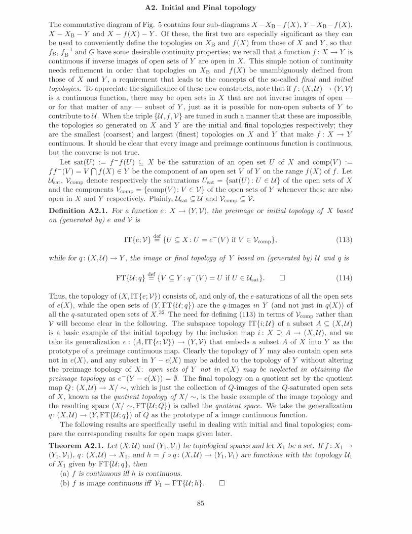
A2. Initial and Final topology

The commutative diagram of Fig. 5 contains four sub-diagrams X−XB−f(X), Y −XB−f(X),X −XB − Y and X − f(X) − Y . Of these, the first two are especially significant as they canbe used to conveniently define the topologies on XB and f(X) from those of X and Y , so thatfB, f−1

B and G have some desirable continuity properties; we recall that a function f : X → Y iscontinuous if inverse images of open sets of Y are open in X. This simple notion of continuityneeds refinement in order that topologies on XB and f(X) be unambiguously defined fromthose of X and Y , a requirement that leads to the concepts of the so-called final and initialtopologies. To appreciate the significance of these new constructs, note that if f : (X,U) → (Y,V)is a continuous function, there may be open sets in X that are not inverse images of open —or for that matter of any — subset of Y , just as it is possible for non-open subsets of Y tocontribute to U . When the triple U , f,V are tuned in such a manner that these are impossible,the topologies so generated on X and Y are the initial and final topologies respectively; theyare the smallest (coarsest) and largest (finest) topologies on X and Y that make f : X → Ycontinuous. It should be clear that every image and preimage continuous function is continuous,but the converse is not true.

Let sat(U) := f−f(U) ⊆ X be the saturation of an open set U of X and comp(V ) :=ff−(V ) = V

⋂f(X) ∈ Y be the component of an open set V of Y on the range f(X) of f . Let

Usat, Vcomp denote respectively the saturations Usat = sat(U) : U ∈ U of the open sets of Xand the components Vcomp = comp(V ) : V ∈ V of the open sets of Y whenever these are alsoopen in X and Y respectively. Plainly, Usat ⊆ U and Vcomp ⊆ V.

Definition A2.1. For a function e : X → (Y,V), the preimage or initial topology of X basedon (generated by) e and V is

ITe;V def= U ⊆ X : U = e−(V ) if V ∈ Vcomp, (113)

while for q : (X,U) → Y , the image or final topology of Y based on (generated by) U and q is

FTU ; q def= V ⊆ Y : q−(V ) = U if U ∈ Usat. (114)

Thus, the topology of (X, ITe;V) consists of, and only of, the e-saturations of all the open setsof e(X), while the open sets of (Y,FTU ; q) are the q-images in Y (and not just in q(X)) ofall the q-saturated open sets of X.32 The need for defining (113) in terms of Vcomp rather thanV will become clear in the following. The subspace topology ITi;U of a subset A ⊆ (X,U)is a basic example of the initial topology by the inclusion map i : X ⊇ A → (X,U), and wetake its generalization e : (A, ITe;V) → (Y,V) that embeds a subset A of X into Y as theprototype of a preimage continuous map. Clearly the topology of Y may also contain open setsnot in e(X), and any subset in Y − e(X) may be added to the topology of Y without alteringthe preimage topology of X: open sets of Y not in e(X) may be neglected in obtaining thepreimage topology as e−(Y − e(X)) = ∅. The final topology on a quotient set by the quotientmap Q : (X,U) → X/ ∼, which is just the collection of Q-images of the Q-saturated open setsof X, known as the quotient topology of X/ ∼, is the basic example of the image topology andthe resulting space (X/ ∼,FTU ;Q) is called the quotient space. We take the generalizationq : (X,U) → (Y,FTU ; q) of Q as the prototype of a image continuous function.

The following results are specifically useful in dealing with initial and final topologies; com-pare the corresponding results for open maps given later.

Theorem A2.1. Let (X,U) and (Y1,V1) be topological spaces and let X1 be a set. If f : X1 →(Y1,V1), q : (X,U) → X1, and h = f q : (X,U) → (Y1,V1) are functions with the topology U1

of X1 given by FTU ; q, then

(a) f is continuous iff h is continuous.

(b) f is image continuous iff V1 = FTU ;h.

85

(X,U)

(Y1,V1)(X1, FTU ; q)

(Y,V)

(Y1, ITe;V)

gh

(X1,U1)

f

f

eq

Figure 21: Continuity in final and initial topologies.

Theorem A2.2. Let (Y,V) and (X1,U1) be topological spaces and let Y1 be a set. If f :(X1,U1) → Y1, e : Y1 → (Y,V) and g = e f : (X1,U1) → (Y,V) are function with the topologyV1 of Y1 given by ITe;V, then

(a) f is continuous iff g is continuous.

(b) f is preimage continuous iff U1 = ITg;V.

As we need the second part of these theorems in our applications, their proofs are indicatedbelow. The special significance of the first parts is that they ensure the converse of the usualresult that the composition of two continuous functions is continuous, namely that one of thecomponents of a composition is continuous whenever the composition is so.

Proof of Theorem A2.1. If f be image continuous, V1 = V1 ⊆ Y1 : f−(V1) ∈ U1 andU1 = U1 ⊆ X1 : q−(U1) ∈ U are the final topologies of Y1 and X1 based on the topologies ofX1 and X respectively. Then V1 = V1 ⊆ Y1 : q−f−(V1) ∈ U shows that h is image continuous.

Conversely, when h is image continuous, V1 = V1 ⊆ Y1 : h−(V1) ∈ U = V1 ⊆ Y1 :q−f−(V1) ∈ U, with U1 = U1 ⊆ X1 : q−(U1) ∈ U, proves f−(V1) to be open in X1 andthereby f to be image continuous.

Proof of Theorem A2.2. If f be preimage continuous, V1 = V1 ⊆ Y1 : V1 = e−(V ) if V ∈ Vand U1 = U1 ⊆ X1 : U1 = f−(V1) if V1 ∈ V1 are the initial topologies of Y1 andX1 respectively.Hence from U1 = U1 ⊆ X1 : U1 = f−e−(V ) if V ∈ V it follows that g is preimage continuous.

Conversely, when g is preimage continuous, U1 = U1 ⊆ X1 : U1 = g−(V ) if V ∈ V =U1 ⊆ X1 : U1 = f−e−(V ) if V ∈ V and V1 = V1 ⊆ Y1 : V1 = e−(V ) if V ∈ V shows that f ispreimage continuous.

Since both Eqs. (113) and (114) are in terms of inverse images (the first of which constitutesa direct, and the second an inverse, problem) the image f(U) = comp(V ) for V ∈ V is of interestas it indicates the relationship of the openness of f with its continuity. This, and other relatedconcepts are examined below, where the range space f(X) is always taken to be a subspace ofY . Openness of a function f : (X,U) → (Y,V) is the “inverse” of continuity, when images ofopen sets of X are required to be open in Y ; such a function is said to be open. Following aretwo of the important properties of open functions.

(1) If f : (X,U) → (Y, f(U)) is an open function, then so is f< : (X,U) → (f(X), ITi; f(U)).The converse is true if f(X) is an open set of Y ; thus openness of f< : (X,U) → (f(X), f<(U))implies that of f : (X,U) → (Y,V) whenever f(X) is open in Y such that f<(U) ∈ V for U ∈ U .

32We adopt the convention of denoting arbitrary preimage and image continuous functions by e and qrespectively even though they are not be injective or surjective; recall that the embedding e : X ⊇ A→ Yand the association q : X → f(X) are 1 : 1 and onto respectively.

86

The truth of this last assertion follows easily from the fact that if f<(U) is an open set off(X) ⊂ Y , then necessarily f<(U) = V

⋂f(X) for some V ∈ V, and the intersection of two

open sets of Y is again an open set of Y .(2) If f : (X,U) → (Y,V) and g : (Y,V) → (Z,W) are open functions then g f : (X,U) →

(Z,W) is also open. It follows that the condition in (1) on f(X) can be replaced by therequirement that the inclusion i : (f(X), ITi;V) → (Y,V) be an open map. This interchangeof f(X) with its inclusion i : f(X) → Y into Y is a basic result that finds application in manysituations.

Collected below are some useful properties of the initial and final topologies that we needin this work.

Initial Topology. In Fig. 21(b), consider Y1 = h(X1), e → i and f → h< : X1 →(h(X1), ITi;V). From h−(B) = h−(B

⋂h(X1)) for any B ⊆ Y , it follows that for an open

set V of Y , h−(Vcomp) = h−(V ) is an open set of X1 which, if the topology of X1 is ITh;V,are the only open sets of X1. Because Vcomp is an open set of h(X1) in its subspace topology,this implies that the preimage topologies ITh;V and ITh<; ITi;V of X1 generated by hand h< are the same. Thus the preimage topology of X1 is not affected if Y is replaced by thesubspace h(X1), the part Y − h(X1) contributing nothing to ITh;V.

A preimage continuous function e : X → (Y,V) is not necessarily an open function. Indeed,if U = e−(V ) ∈ ITe;V, it is almost trivial to verify along the lines of the restriction of openmaps to its range, that e(U) = ee−(V ) = e(X)

⋂V , V ∈ V, is open in Y (implying that e is an

open map) iff e(X) is an open subset of Y (because finite intersections of open sets are open).A special case of this is the important consequence that the restriction e< : (X, ITe;V) →(e(X), ITi;V) of e : (X, ITh;V) → (Y,V) to its range is an open map. Even though apreimage continuous map need not be open, it is true that an injective, continuous and openmap f : X → (Y,V) is preimage continuous. Indeed, from its injectivity and continuity, inverseimages of all open subsets of Y are saturated-open in X, and openness of f ensures that theseare the only open sets of X the condition of injectivity being required to exclude non-saturatedsets from the preimage topology. It is therefore possible to rewrite Eq. (113) as

U ∈ ITe;V ⇐⇒ e(U) = V if V ∈ Vcomp, (115)

and to compare it with the following criterion for an injective, open-continuous map f : (X,U) →(Y,V) that necessarily satisfies sat(A) = A for all A ⊆ X

U ∈ U ⇐⇒ (f(U)U∈U = Vcomp) ∧ (f−1(V )|V ∈V ∈ U). (116)

Final Topology. Since it is necessarily produced on the range R(q) of q, the final topology isoften considered in terms of a surjection. This however is not necessary as, much in the spiritof the initial topology, Y − q(X) 6= ∅ inherits the discrete topology without altering anything,thereby allowing condition (114) to be restated in the following more transparent form

V ∈ FTU ; q ⇐⇒ V = q(U) if U ∈ Usat, (117)

and to compare it with the following criterion for a surjective, open-continuous map f : (X,U) →(Y,V) that necessarily satisfies fB = B for all B ⊆ Y

V ∈ V ⇐⇒ (Usat = f−(V )V ∈V) ∧ (f(U)|U∈U ∈ V). (118)

As may be anticipated from Fig. 21, the final topology does not behave as well for subspaces asthe initial topology does. This is so because in Fig. 21(a) the two image continuous functions hand q are connected by a preimage continuous inclusion f , whereas in Fig. 21(b) all the threefunctions are preimage continuous. Thus quite like open functions, although image continuityof h : (X,U) → (Y1,FTU ;h) implies that of h< : (X,U) → (h(X), ITi; FTU ;h)) for asubspace h(X) of Y1, the converse need not be true unless — entirely like open functions again

87

— either h(X) is an open set of Y1 or i : (h(X), ITi; FTU ;h)) → (X,FTU ;h) is an openmap. Since an open preimage continuous map is image continuous, this makes i : h(X) → Y1

an ininal function and hence all the three legs of the commutative diagram image continuous.

Like preimage continuity, an image continuous function q : (X,U) → Y need not be open.However, although the restriction of an image continuous function to the saturated open setsof its domain is an open function, q is unrestrictedly open iff the saturation of every open setof X is also open in X. Infact it can be verified without much effort that a continuous, opensurjection is image continuous.

Combining Eqs. (115) and (117) gives the following criterion for ininality

U and V ∈ IFTUsat; f ;V ⇐⇒ (f(U)U∈Usat= V)(Usat = f−(V )V ∈V), (119)

which reduces to the following for a homeomorphism f that satisfies both sat(A) = A for A ⊆ Xand fB = B for B ⊆ Y

U and V ∈ HOMU ; f ;V ⇐⇒ (U = f−1(V )V ∈V)(f(U)U∈U = V) (120)

and compares with

U and V ∈ OCU ; f ;V ⇐⇒ (sat(U) ∈ U : f(U)U∈U = Vcomp)∧∧ (comp(V ) ∈ V : f−(V )V ∈V = Usat) (121)

for an open-continuous f .

The following is a slightly more general form of the restriction on the inclusion that is neededfor image continuity to behave well for subspaces of Y .

Theorem A2.3. Let q : (X,U) → (Y,FTU ; q) be an image continuous function. For asubspace B of (Y,FTU ; q),

FTITj;U; q< = ITi; FTU ; q

where q< : (q−(B), ITj;U) → (B,FTITj;U; q<), if either q is an open map or B is anopen set of Y .

In summary we have the useful result that an open preimage continuous function is imagecontinuous and an open image continuous function is preimage continuous, where the secondassertion follows on neglecting non-saturated open sets in X; this is permitted in as far as thegeneration of the final topology is concerned, as these sets produce the same images as theirsaturations. Hence an image continuous function q : X → Y is preimage continuous iff everyopen set in X is saturated with respect to q, and a preimage continuous function e : X → Y isimage continuous iff the e-image of every open set of X is open in Y .

A3. More on Topological Spaces

This Appendix — which completes the review of those concepts of topological spaces begun inTutorial4 that are needed for a proper understanding of this work — begins with the followingsummary of the different possibilities in the distribution of Der(A) and Bdy(A) between setsA ⊆ X and its complement X − A, and follows it up with a few other important topologicalconcepts that have been used, explicitly or otherwise, in this work.

Definition A3.1. Separation, Connected Space. A separation (disconnection) of X is apair of mutually disjoint nonempty open (and therefore closed) subsets H1 and H2 such thatX = H1 ∪H2. A space X is said to be connected if it has no separation, that is if it cannot bepartitioned into two open or two closed nonempty subsets. X is separated (disconnected) if itis not connected.

88

2. Selfish (Closed)

X X

1. Donor

2. Selfish(Closed)

3. Neutral

3. Neutral1. Donor

X −A

A

X −A open X −A open

X X

X

X

Der(X −A)BdyX−A(A)Der(A) BdyA(X −A)

A

AA openA

A A open A

A A open

X −A open

Figure 22: Classification of a subset A of X relative to the topology of X . The derived set of A may

intersect both A and X −A (row 3), may be entirely in A (row 2), or may be wholly in X −A (row 1).

A is closed iff Bdy(A) := BdyX−A(A)∪BdyA(X −A) = (Cl(A)∩ (X −A)) ∪ (Cl(X −A)∩A) ⊆ A (row

2), open iff Bdy(A) ⊆ X − A (column 2), and clopen iff Bdy(A) = ∅ when the derived sets of both A

and X − A are contained in the respective sets. An open set, beside being closed, may also be neutral

or donor.

89

It follows from the definition, that for a disconnected space X the following are equivalentstatements.

(a) There exist a pair of disjoint nonempty open subsets of X that cover X.

(b) There exist a pair of disjoint nonempty closed subsets of X that cover X.

(c) There exist a pair of disjoint nonempty clopen subsets of X that cover X.

(d) There exists a nonempty, proper, clopen subset of X.

By a connected subset is meant a subset of X that is connected when provided with its relativetopology making it a subspace of X. Thus any connected subset of a topological space mustnecessarily be contained in any clopen set that might intersect it: if C and H are respectivelyconnected and clopen subsets of X such that C

⋂H 6= ∅, then C ⊂ H because C

⋂H is a

nonempty clopen set in C which must contain C because C is connected.

For testing whether a subset of a topological space is connected, the following relativizedform of (a)−(d) is often useful.

Lemma A3.1. A subset A of X is disconnected iff there are disjoint open sets U and V of Xsatisfying

U⋂A 6= ∅ 6= V

⋂A such that A ⊆ U

⋃V, with U

⋂V⋂A = ∅ (122)

or there are disjoint closed sets E and F of X satisfying

E⋂A 6= ∅ 6= F

⋂A such that A ⊆ E

⋃F, with E

⋂F⋂A = ∅. (123)

Thus A is disconnected iff there are disjoint clopen subsets in the relative topology of A thatcover A.

Lemma A3.2. If A is a subspace of X, a separation of A is a pair of disjoint nonempty subsetsH1 and H2 of A whose union is A neither of which contains a cluster point of the other. A isconnected iff there is no separation of A.

Proof. Let H1 and H2 be a separation of A so that they are clopen subsets of A whose unionis A. As H1 is a closed subset of A it follows that H1 = ClX(H1)

⋂A, where ClX(H1)

⋂A is

the closure of H1 in A; hence ClX(H1)⋂H2 = ∅. But as the closure of a subset is the union

of the set and its adherents, an empty intersection signifies that H2 cannot contain any of thecluster points of H1. A similar argument shows that H1 does not contain any adherent of H2.

Conversely suppose that neitherH1 norH2 contain an adherent of the other: ClX(H1)⋂H2 =

∅ and ClX(H2)⋂H1 = ∅. Hence ClX(H1)

⋂A = H1 and ClX(H2)

⋂A = H2 so that both H1

and H2 are closed in A. But since H1 = A−H2 and H2 = A−H1, they must also be open inthe relative topology of A.

Following are some useful properties of connected spaces.

(c1) The closure of any connected subspace of a space is connected. In general, every Bsatisfying

A ⊆ B ⊆ Cl(A)

is connected. Thus any subset of X formed from A by adjoining to it some or all of its adherentsis connected so that a topological space with a dense connected subset is connected.

(c2) The union of any class of connected subspaces of X with nonempty intersection is aconnected subspace of X.

(c3) A topological space is connected iff there is a covering of the space consisting of con-nected sets with nonempty intersection. Connectedness is a topological property: Any spacehomeomorphic to a connected space is itself connected.

(c4) If H1 and H2 is a separation of X and A is any connected subset A of X, then eitherA ⊆ H1 or A ⊆ H2.

While the real line R is connected, a subspace of R is connected iff it is an interval in R.

The important concept of total disconnectedness introduced below needs the following

90

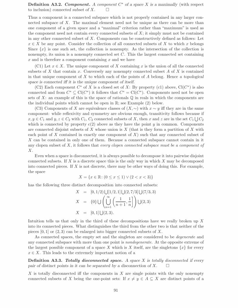
Definition A3.2. Component . A component C∗ of a space X is a maximally (with respectto inclusion) connected subset of X.

Thus a component is a connected subspace which is not properly contained in any larger con-nected subspace of X. The maximal element need not be unique as there can be more thanone component of a given space and a “maximal” criterion rather than “maximum” is used asthe component need not contain every connected subsets of X; it simply must not be containedin any other connected subset of X. Components can be constructively defined as follows: Letx ∈ X be any point. Consider the collection of all connected subsets of X to which x belongsSince x is one such set, the collection is nonempty. As the intersection of the collection isnonempty, its union is a nonempty connected set C. This the largest connected set containingx and is therefore a component containing x and we have

(C1) Let x ∈ X. The unique component of X containing x is the union of all the connectedsubsets of X that contain x. Conversely any nonempty connected subset A of X is containedin that unique component of X to which each of the points of A belong. Hence a topologicalspace is connected iff it is the unique component of itself.

(C2) Each component C∗ of X is a closed set of X: By property (c1) above, Cl(C∗) is alsoconnected and from C∗ ⊆ Cl(C∗) it follows that C∗ = Cl(C∗). Components need not be opensets of X: an example of this is the space of rationals Q in reals in which the components arethe individual points which cannot be open in R; see Example (2) below.

(C3) Components of X are equivalence classes of (X,∼) with x ∼ y iff they are in the samecomponent: while reflexivity and symmetry are obvious enough, transitivity follows because ifx, y ∈ C1 and y, z ∈ C2 with C1, C2 connected subsets of X, then x and z are in the set C1

⋃C2

which is connected by property c(2) above as they have the point y in common. Componentsare connected disjoint subsets of X whose union is X (that is they form a partition of X witheach point of X contained in exactly one component of X) such that any connected subset ofX can be contained in only one of them. Because a connected subspace cannot contain in itany clopen subset of X, it follows that every clopen connected subspace must be a component ofX.

Even when a space is disconnected, it is always possible to decompose it into pairwise disjointconnected subsets. If X is a discrete space this is the only way in which X may be decomposedinto connected pieces. If X is not discrete, there may be other ways of doing this. For example,the space

X = x ∈ R : (0 ≤ x ≤ 1) ∨ (2 < x < 3)has the following three distinct decomposition into connected subsets:

X = [0, 1/2)⋃

[1/2, 1]⋃

(2, 7/3]⋃

(7/3, 3)

X = 0⋃(∞⋃

n=1

(1

n+ 1,1

n

])⋃(2, 3)

X = [0, 1]⋃

(2, 3).

Intuition tells us that only in the third of these decompositions have we really broken up Xinto its connected pieces. What distinguishes the third from the other two is that neither of thepieces [0, 1] or (2, 3) can be enlarged into bigger connected subsets of X.

As connected spaces, the empty set and the singleton are considered to be degenerate andany connected subspace with more than one point is nondegenerate. At the opposite extreme ofthe largest possible component of a space X which is X itself, are the singletons x for everyx ∈ X. This leads to the extremely important notion of a

Definition A3.3. Totally disconnected space. A space X is totally disconnected if everypair of distinct points in it can be separated by a disconnection of X.

X is totally disconnected iff the components in X are single points with the only nonemptyconnected subsets of X being the one-point sets: If x 6= y ∈ A ⊆ X are distinct points of a

91

subset A of X then A = (A⋂H1)

⋃(A⋂H2), where X = H1

⋃H2 with x ∈ H1 and y ∈ H2 is a

disconnection of X (it is possible to choose H1 and H2 in this manner because X is assumed tobe totally disconnected), is a separation of A that demonstrates that any subspace of a totallydisconnected space with more than one point is disconnected.

A totally disconnected space has interesting physically appealing separation properties interms of the (separated) Hausdorff spaces; here a topological space X is Hausdorff, or T2, iffeach two distinct points of X can be separated by disjoint neighbourhoods, so that for everyx 6= y ∈ X, there are neighbourhoods M ∈ Nx and N ∈ Ny such that M

⋂N = ∅. This means

that for any two distinct points x 6= y ∈ X, it is impossible to find points that are arbitrarilyclose to both of them. Among the properties of Hausdorff spaces, the following need to bementioned.

(H1) X is Hausdorff iff for each x ∈ X and any point y 6= x, there is a neighbourhood Nof x such that y 6∈ Cl(N). This leads to the significant result that for any x ∈ X the closedsingleton

x =⋂

N∈Nx

Cl(N)

is the intersection of the closures of any local base at that point, which in the language of netsand filters (Appendix A1) means that a net in a Hausdorff space cannot converge to more thanone point in the space and the adherent set adh(Nx) of the neighbourhood filter at x is thesingleton x.

(H2) Since each singleton is a closed set, each finite set in a Hausdorff space is also closedin X. Unlike a cofinite space, however, there can clearly be infinite closed sets in a Hausdorffspace.

(H3) Any point x in a Hausdorff space X is a cluster point of A ⊆ X iff every neighbourhoodof x contains infinitely many points of A, a fact that has led to our mental conditioning of thepoints of a (Cauchy) sequence piling up in neighbourhoods of the limit. Thus suppose forthe sake of argument that although some neighbourhood of x contains only a finite numberof points, x is nonetheless a cluster point of A. Then there is an open neighbourhood U ofx such that U

⋂(A − x) = x1, · · · , xn is a finite closed set of X not containing x, and

U⋂

(X − x1, · · · , xn) being the intersection of two open sets, is an open neighbourhood ofx not intersecting A − x implying thereby that x 6∈ Der(A); infact U

⋂(X − x1, · · · , xn)

is simply x if x ∈ A or belongs to BdyX−A(A) when x ∈ X − A. Conversely if everyneighbourhood of a point of X intersects A in infinitely many points, that point must belongto Der(A) by definition.

Weaker separation axioms than Hausdorffness are those of T0, respectively T1, spaces inwhich for every pair of distinct points at least one, respectively each one, has some neighbour-hood not containing the other; the following table is a listing of the separation properties ofsome useful spaces.

It should be noted that that as none of the properties (H1)–(H3) need neighbourhoods ofboth the points simultaneously, it is sufficient for X to be T1 for the conclusions to remain valid.

From its definition it follows that any totally disconnected space is a Hausdorff space andis therefore both T1 and T0 spaces as well. However, if a Hausdorff space has a base of clopensets then it is totally disconnected; this is so because if x and y are distinct points of X,then the assumed property of x ∈ H ⊆ M for every M ∈ Nx and some clopen set M yieldsX = H

⋃(X − H) as a disconnection of X that separates x and y ∈ X − H; note that the

assumed Hausdorffness of X allows M to be chosen so as not to contain y.

Example A3.1. (1) Every indiscrete space is connected; every subset of an indiscrete space isconnected. Hence if X is empty or a singleton, it is connected. A discrete space is connectediff it is either empty or is a singleton; the only connected subsets in a discrete space are thedegenerate ones. This is an extreme case of lack of connectedness, and a discrete space is thesimplest example of a total disconnected space.

92

Space T0 T1 T2

Discrete X X X

Indiscrete × × ×R, standard X X X

left/right ray X × ×Infinite cofinite X X ×

Uncountable cocountable X X ×x-inclusion/exclusion X × ×A-inclusion/exclusion × × ×

Table 7: Separation properties of some useful spaces.

(2) Q, the set of rationals considered as a subspace of the real line, is (totally) disconnectedbecause all rationals larger than a given irrational r is a clopen set in Q, and

Q = ((−∞, r)⋂

Q)⋃

(Q⋂

(r,∞)) r is an irrational

is the union of two disjoint clopen sets in the relative topology of Q. The sets (−∞, r) ∩ Q

and Q ∩ (r,∞) are clopen in Q because neither contains a cluster point of the other. Thus forexample, any neighbourhood of the second must contain the irrational r in order to be able tocut the first which means that any neighbourhood of a point in either of the relatively open setscannot be wholly contained in the other. The only connected sets of Q are one point subsetsconsisting of the individual rationals. In fact, a connected piece of Q, being a connected subsetof R, is an interval in R, and a nonempty interval cannot be contained in Q unless it is asingleton. It needs to be noted that the individual points of the rational line are not (cl)openbecause any open subset of R that contains a rational must also contain others different from it.This example shows that a space need not be discrete for each of its points to be a componentand thereby for the space to be totally disconnected.

In a similar fashion, the set of irrationals is (totally) disconnected because all the irrationalslarger than a given rational is an example of a clopen set in R − Q.

(3) The p-inclusion (A-inclusion) topology is connected; a subset in this topology is connectediff it is degenerate or contains p. For, a subset inherits the discrete topology if it does not containp, and p-inclusion topology if it contains p.

(4) The cofinite (cocountable) topology on an infinite (uncountable) space is connected; asubset in a cofinite (cocountable) space is connected iff it is degenerate or infinite (countable).

(5) Removal of a single point may render a connected space disconnected and even totallydisconnected. In the former case, the point removed is called a cut point and in the second, itis a dispersion point. Any real number is a cut point of R and it does not have any dispersionpoint only.

(6) Let X be a topological space. Considering components of X as equivalence classes bythe equivalence relation ∼ with Q : X → X/ ∼ denoting the quotient map, X/ ∼ is totallydisconnected: As Q−([x]) is connected for each [x] ∈ X/ ∼ in a component class of X, and asany open or closed subset A ⊆ X/ ∼ is connected iff Q−(A) is open or closed, it must followthat A can only be a singleton.

The next notion of compactness in topological spaces provides an insight of the role ofnonempty adherent sets of filters that lead in a natural fashion to the concept of attractors inthe dynamical systems theory that we take up next.

Definition A3.4. Compactness. A topological space X is compact iff every open cover of Xcontains a finite subcover of X.

93

This definition of compactness has an useful equivalent contrapositive reformulation: For anygiven collection of open sets of X if none of its finite subcollections cover X, then the entirecollection also cannot cover X. The following theorem is a statement of the fundamental prop-erty of compact spaces in terms of adherences of filters in such spaces, the proof of which usesthis contrapositive characterization of compactness.

Theorem A3.1. A topological space X is compact iff each class of closed subsets of X withfinite intersection property has nonempty intersection.

Proof. Necessity. Let X be a compact space. Let F = Fαα∈D be a collection of closedsubsets of X with finite FIP, and let G = X − Fαα∈D be the corresponding open sets of X.If GiN

i=1 is a nonempty finite subcollection from G, then X − GiNi=1 is the corresponding

nonempty finite subcollection of F . Hence from the assumed finite intersection property of F ,it must be true that

X −N⋃

i=1

Gi =

N⋂

i=1

(X −Gi) (DeMorgan′s Law)

6= ∅,

so that no finite subcollection of G can cover X. Compactness of X now implies that G toocannot cover X and therefore

⋂

α

Fα =⋂

α

(X −Gα) = X −⋃

α

Gα 6= ∅.

The proof of the converse is a simple exercise of reversing the arguments involving the twoequations in the proof above.

Our interest in this theorem and its proof lies in the following corollary — which essentiallymeans that for every filter F on a compact space the adherent set adh(F) is not empty — fromwhich follows that every net in a compact space must have a convergent subnet.

Corollary. A space X is compact iff for every class A = (Aα) of nonempty subsets of X withFIP, adh(A) =

⋂Aα∈A

Cl(Aα) 6= ∅.

The proof of this result for nets given by the next theorem illustrates the general approach insuch cases which is all that is basically needed in dealing with attractors of dynamical systems;compare Theorem A1.3.

Theorem A3.2. A topological space X is compact iff each net in X adheres in X.

Proof. Necessity. Let X be a compact space, χ : D → X a net in X, and Rα the residual of αin the directed set D. For the filter-base (FBχ(Rα))α∈D of nonempty, decreasing, nested subsetsof X associated with the net χ, compactness of X requires from

⋂αδ Cl(χ(Rα) ⊇ χ(Rδ) 6= ∅,

that the uncountably intersecting subset

adh(FBχ) :=⋂

α∈D

Cl(χ(Rα))

of X be non-empty. If x ∈ adh(FBχ) then because x is in the closure of χ(Rβ), it follows fromEq. (20) that N

⋂χ(Rβ) 6= ∅33 for every N ∈ Nx, β ∈ D. Hence χ(γ) ∈ N for some γ β so

that x ∈ adh(χ); see Eq. (88).Sufficiency. Let χ be a net in X that adheres at x ∈ X. From any class F of closed subsets

of X with FIP, construct as in the proof of Thm. A1.4, a decreasing nested sequence of closedsubsets Cβ =

⋂αβ∈DFα : Fα ∈ F and consider the directed set DCβ = (Cβ , β) : (β ∈

D)(xβ ∈ Cβ) with its natural direction (83) to define the net χ(Cβ, β) = xβ in X; see Def.A1.10. From the assumed adherence of χ at some x ∈ X, it follows that N

⋂F 6= ∅ for every

33This is of course a triviality if we identify each χ(Rβ) (or F in the proof of the converse that follows)with a neighbourhood N of X that generates a topology on X .

94

N ∈ Nx and F ∈ F . Hence x belongs to the closed set F so that x ∈ adh(F); see Eq. (96).Hence X is compact.

Using Theorem A1.5 that specifies a definite criterion for the adherence of a net, this theoremreduces to the useful formulation that a space is compact iff each net in it has some convergentsubnet. An important application is the following: Since every decreasing sequence (Fm) ofnonempty sets has FIP (because

⋂Mm=1 Fm = FM for every finite M), every decreasing sequence

of nonempty closed subsets of a compact space has nonempty intersection. For a complete metricspace this is known as the Nested Set Theorem, and for [0, 1] and other compact subspaces ofR as the Cantor Intersection Theorem.34

For subspaces A of X, it is the relative topology that determines as usual compactness of A;however the following criterion renders this test in terms of the relative topology unnecessaryand shows that the topology of X itself is sufficient to determine compactness of subspaces: Asubspace K of a topological space X is compact iff each open cover of K in X contains a finitecover of K.

A proper understanding of the distinction between compactness and closedness of subspaces— which often causes much confusion to the non-specialist — is expressed in the next twotheorems. As a motivation for the first that establishes that not every subset of a compactspace need be compact, mention may be made of the subset (a, b) of the compact closed interval[a, b] in R.

Theorem A3.3. A closed subset F of a compact space X is compact.

Proof. Let G be an open cover of F so that an open cover of X is G⋃(X −F ), which becauseof compactness of X contains a finite subcover U . Then U − (X − F ) is a finite collection of Gthat covers F .

It is not true in general that a compact subset of a space is necessarily closed. For example,in an infinite set X with the cofinite topology, let F be an infinite subset of X with X −F alsoinfinite. Then although F is not closed in X, it is nevertheless compact because X is compact.Indeed, let G be an open cover of X and choose any nonempty G0 ∈ G. If G0 = X thenG0 is the required finite cover of X. If this is not the case, then because X −G0 = xin

i=1

is a finite set, there is a Gi ∈ G with xi ∈ Gi for each 1 ≤ i ≤ n, and therefore Gini=0 is

the finite cover that demonstrates the compactness of the cofinite space X. Compactness of Fnow follows because the subspace topology on F is the induced cofinite topology from X. Thedistinguishing feature of this topology is that it, like the cocountable, is not Hausdorff: If Uand V are any two nonempty open sets of X, then they cannot be disjoint as the complementsof the open sets can only be finite and if U

⋂V were to be indeed empty, then

X = X − ∅ = X − (U⋂V ) = (X − U)

⋃(X − V )

would be a finite set. An immediate fallout of this is that in an infinite cofinite space, asequence (xi)i∈N (and even a net) with xi 6= xj for i 6= j behaves in an extremely unusual way:It converges, as in the indiscrete space, to every point of the space. Indeed if x ∈ X, where X isan infinite set provided with its cofinite topology, and U is any neighbourhood of x, any infinitesequence (xi)i∈N in X must be eventually in U because X − U is finite, and ignoring of theinitial set of its values lying in X − U in no way alters the ultimate behaviour of the sequence(note that this implies that the filter induced on X by the sequence agrees with its topology).

34Nested-set theorem. If (En) is a decreasing sequence of nonempty, closed, subsets of a complete

metric space (X, d) such that limn→∞ dia(En) = 0, then there is a unique point

x ∈∞⋂

n=0

En.

The uniqueness arises because the limiting condition on the diameters of En imply, from property (H1),that (X, d) is a Hausdorff space.

95

Thus xi → x for any x ∈ X is a reflection of the fact that there are no small neighbourhoodsof any point of X with every neighbourhood being almost the whole of X, except for a null setconsisting of only a finite number of points. This is in sharp contrast with Hausdorff spaceswhere, although every finite set is also closed, every point has arbitrarily small neighbourhoodsthat lead to unique limits of sequences. A corresponding result for cocountable spaces can befound in Example A1.2 Continued.

This example of the cofinite topology motivates the following “converse” of the previoustheorem.

Theorem A3.4. Every compact subspace of a Hausdorff space is closed.

.

.

x

Hausdorff X

VyUy

y

V

compact K

Figure 23: Closedness of compact subsets of a Hausdorff space.

Proof. Let K be a nonempty compact subset of X, Fig. 23, and let x ∈ X−K. Because of theseparation of X, for every y ∈ K there are disjoint open subsets Uy and Vy of X with y ∈ Uy,and x ∈ Vy. Hence Uyy∈K is an open cover for K, and from its compactness there is a finitesubset A of K such that K ⊆ ⋃

y∈A Uy with V =⋂

y∈A Vy an open neighbourhood of x; V isopen because each Vy is a neighbourhood of x and the intersection is over finitely many pointsy of A. To prove that K is closed in X it is enough to show that V is disjoint from K: If thereis indeed some z ∈ V

⋂K then z must be in some Uy for y ∈ A. But as z ∈ V it is also in Vy

which is impossible as Uy and Vy are to be disjoint. This last part of the argument infact showsthat if K is a compact subspace of a Hausdorff space X and x /∈ K, then there are disjoint opensets U and V of X containing x and K.

The last two theorems may be combined to give the obviously important

Corollary. In a compact Hausdorff space, closedness and compactness of its subsets are equiv-alent concepts.

In the absence of Hausdorffness, it is not possible to conclude from the assumed compactnessof the space that every point to which the net may converge actually belongs to the subspace.

Definition A3.5. A subset D of a topological space (X,U) is dense in X if Cl(D) = X. Thusthe closure of D is the largest open subset of X, and every neighbourhood of any point of Xcontains a point of D not necessarily distinct from it; refer to the distinction between Eqs. (20)and (22).

Loosely, D is dense in X iff every point of X has points of D arbitrarily close to it. Aself-dense (dense in itself ) set is a set without any isolated points; hence A is self-dense iffA ⊆ Der(A). A closed self-dense set is called a perfect set so that a closed set A is perfect iff ithas no isolated points. Accordingly

A is perfect ⇐⇒ A = Der(A),

96

means that the closure of a set without any isolated points is a perfect set.

Theorem A3.5. The following are equivalent statements.(1) D is dense in X.(2) If F is any closed set of X with D ⊆ F , then F = X; thus the only closed superset of D

is X.(3) Every nonempty (basic) open set of X cuts D; thus the only open set disjoint from D is

the empty set ∅.(4) The exterior of D is empty.

Proof. (3) If U indeed is a nonempty open set of X with U⋂D = ∅, then D ⊆ X − U 6= X

leads to the contradiction X = Cl(D) ⊆ Cl(X − U) = X − U 6= X, which also incidentallyproves (2). From (3) it follows that for any open set U of X, Cl(U) = Cl(U

⋂D) because if V

is any open neighbourhood of x ∈ Cl(U) then V⋂U is a nonempty open set of X that must

cut D so that V⋂

(U⋂D) 6= ∅ implies x ∈ Cl(U

⋂D). Finally, Cl(U

⋂D) ⊆ Cl(U) completes

the proof.

Definition A3.6. (a) A set A ⊆ X is said to be nowhere dense in X if Int(Cl(A)) = ∅ andresidual in X if Int(A) = ∅.

A is nowhere dense in X iff

Bdy(X − Cl(A)) = Bdy(Cl(A)) = Cl(A)

so thatCl(X − Cl(A)) = (X − Cl(A))

⋃Cl(A) = X

from which it follows that

A is nwd in X ⇐⇒ X − Cl(A) is dense in X

andA is residual in X ⇐⇒ X −A is dense in X.

Thus A is nowhere dense iff Ext(A) := X − Cl(A) is dense in X, and in particular a closedset is nowhere dense in X iff its complement is open dense in X with open-denseness beingcomplimentarily dual to closed-nowhere denseness. The rationals in reals is an example of a setthat is residual but not nowhere dense. The following are readily verifiable properties of subsetsof X.

(1) A set A ⊆ X is nowhere dense in X iff it is contained in its own boundary, iff it iscontained in the closure of the complement of its closure, that is A ⊆ Cl(X − Cl(A)). Inparticular a closed subset A is nowhere dense in X iff A = Bdy(A), that is iff it contains noopen set.

(2) From M ⊆ N ⇒ Cl(M) ⊆ Cl(N) it follows, with M = X −Cl(A) and N = X −A, thata nowhere dense set is residual, but a residual set need not be nowhere dense unless it is alsoclosed in X.

(3) Since Cl(Cl(A)) = Cl(A), Cl(A) is nowhere dense in X iff A is.(4) For anyA ⊆ X, both BdyA(X−A) := Cl(X−A)

⋂A and BdyX−A(A) := Cl(A)

⋂(X−A)

are residual sets and as Fig. 22 shows

BdyX(A) = BdyX−A(A)⋃

BdyA(X −A)

is the union of these two residual sets. When A is closed (or open) in X, its boundary consistingof the only component BdyA(X −A) (or BdyX−A(A)) as shown by the second row (or column)of the figure, being a closed set of X is also nowhere dense in X; infact a closed nowhere denseset is always the boundary of some open set. Otherwise, the boundary components of the tworesidual parts — as in the donor-donor, donor-neutral, neutral-donor and neutral-neutral cases— need not be individually closed in X (although their union is) and their union is a residual

97

set that need not be nowhere dense in X: the union of two nowhere dense sets is nowheredense but the union of a residual and a nowhere dense set is a residual set. One way in whicha two-component boundary can be nowhere dense is by having BdyA(X − A) ⊇ Der(A) orBdyX−A(A) ⊇ Der(X −A), so that it is effectively in one piece rather than in two, as shown inFig. 24(b).

(d) A is Cantor

A

X X

A

X X

(b) A is nwd

A A

(c) Bdy(A) is nwd

= Der(C(A))

Der(A) = Bdy(A)Der(A) = ∅(a) A is isolated

Bdy(C(Cl(A))) = Cl(A)

Der(C(A)) ⊆ C(A) = Bdy(C(A))

Der(A) = A

= Bdy(Cl(A))

Figure 24: Shows the distinction between isolated, nowhere dense and Cantor sets. Topologically, the

Cantor set can be described as a perfect, nowhere dense, totally disconnected and compact subset of

a space. In (b), the closed nowhere dense set Cl(A) is the boundary of its open complement. Here

downward and upward inclined hatching denote respectively BdyA(X −A) and BdyX−A(A).

Theorem A3.6. A is nowhere dense in X iff each non-empty open set of X has a non-emptyopen subset disjoint from Cl(A).

Proof. If U is a nonempty open set of X, then U0 = U∩Ext(A) 6= ∅ as Ext(A) is dense in X; U0

is the open subset that is disjoint from Cl(A). It clearly follows from this that each non-emptyopen set of X has a non-empty open subset disjoint from a nowhere dense set A.

What this result (which follows just from the definition of nowhere dense sets) actuallymeans is that no point in BdyX−A(A) can be isolated in it.

Corollary. A is nowhere dense in X iff Cl(A) does not contain any nonempty open set of Xiff any nonempty open set that contains A also contains its closure.

Example A3.2. Each finite subset of Rn is nowhere dense in Rn; the set 1/n∞n=1 is nowheredense in R. The Cantor set C is nowhere dense in [0, 1] because every neighbourhood of anypoint in C must contain, by its very construction, a point with 1 in its ternary representation.That the interior and the interior of the closure of a set are not necessarily the same is seen inthe example of the rationals in reals: The set of rational numbers Q has empty interior becauseany neighbourhood of a rational number contains irrational numbers (so also is the case forirrational numbers) and R = Int(Cl(Q)) ⊇ Int(Q) = ∅ justifies the notion of a nowhere denseset.

The following properties of C can be taken to define any subset of a topological space as aCantor set; set-theoretically it should be clear from its classical middle-third construction thatthe Cantor set consists of all points of the closed interval [0, 1] whose infinite triadic (base 3)representation, expressed so as not to terminate with an infinite string of 1’s, does not containthe digit 1. Accordingly, any end-point of the infinite set of closed intervals whose intersectionyields the Cantor set, is represented by a repeating string of either 0 or 2 while a non end-pointhas every other arbitrary collection of these two digits. Recalling that any number in [0, 1]is a rational iff its representation in any base is terminating or recurring — thus any decimalthat neither repeats or terminates but consists of all possible sequences of all possible digits

98

represents an irrational number — it follows that both rationals and irrationals belong to theCantor set.

. .

. .

. . . .

. . ..

C0

x(1)3

C3

C2

C4

C1

x(0)2

x(2)2 x

(2)7x

(2)6

x(0)1

C

x(1)2x

(1)1

x(2)4 x

(2)5 x

(2)8

x(3)16

x(2)3

x(2)1

x(3)4 x

(3)5 x

(3)12x

(3)1 x

(3)13

x(1)4

x(3)8 x

(3)9

Figure 25: Construction of the classical 1/3-Cantor set. The endpoints of C3, for example, in increasing

order are:∣∣0, 1

27

∣∣ ;∣∣ 227 ,

19

∣∣ ;∣∣29 ,

727

∣∣ ;∣∣ 827 ,

13

∣∣ ;∣∣23 ,

1927

∣∣ ;∣∣2027 ,

79

∣∣ ;∣∣89 ,

2527

∣∣ ;∣∣ 2627 , 1

∣∣. Ci is the union of 2i pairwise

disjoint closed intervals each of length 3−i and the nonempty infinite intersection C = ∩∞i=0Ci is the

adherent Cantor set of the filter-base of closed sets C0, C1, C2, · · · .

(C1) C is totally disconnected. If possible, let C have a component containing points aand b with a < b. Then [a, b] ⊆ C ⇒ [a, b] ⊆ Ci for all i. But this is impossible because we maychoose i large enough to have 3−i < b−a so that a and b must belong to two different membersof the pairwise disjoint closed 2i subintervals each of length 3−i that constitutes Ci. Hence

[a, b] is not a subset of any Ci =⇒ [a, b] is not a subset of C.

(C2) C is perfect so that for any x ∈ C every neighbourhood of x must contain some otherpoint of C. Supposing to the contrary that the singleton x is an open set of C, there must bean ε > 0 such that in the usual topology of R

x = C⋂(x− ε, x+ ε). (124)

Choose a positive integer i large enough to satisfy 3−i < ε. Since x is in every Ci, it must bein one of the 2i pairwise disjoint closed intervals [a, b] ⊂ (x− ε, x+ ε) each of length 3−i whoseunion is Ci. As [a, b] is an interval, at least one of the endpoints of [a, b] is different from x, andsince an endpoint belongs to C, C ∩ (x− ε, x+ ε) must also contain this point thereby violatingEq. (124).

(C3) C is nowhere dense because each neighbourhood of any point of C intersects Ext(C);see Thm. A3.6.

(C4) C is compact because it is a closed subset contained in the compact subspace [0, 1]of R, see Thm. A3.3. The compactness of [0, 1] follows from the Heine-Borel Theorem whichstates that any subset of the real line is compact iff it is both closed and bounded with respectto the Euclidean metric on R.

Compare (C1) and (C2) with the essentially similar arguments of Example A3.1(2) for thesubspace of rationals in R.

A4. Neutron Transport Theory

This section introduces the reader to the basics of the linear neutron transport theory wheregraphical convergence approximations to the singular distributions, interpreted here as multi-functions, led to the present study of this work. The one-speed (that is mono-energetic) neutron

99

transport equation in one dimension and plane geometry, is

µ∂Φ(x, µ)

∂x+ Φ(x, µ) =

c

2

∫ 1

−1Φ(x, µ′)dµ′, 0 < c < 1, −1 ≤ µ ≤ 1 (125)

where x is a non-dimensional physical space variable that denotes the location of the neutronmoving in a direction θ = cos−1(µ), Φ(x, µ) is a neutron density distribution function such thatΦ(x, µ)dxdµ is the expected number of neutrons in a distance dx about the point x moving atconstant speed with their direction cosines of motion in dµ about µ, and c is a physical constantthat will be taken to satisfy the restriction shown above. Case’s method starts by assuming thesolution to be of the form Φν(x, µ) = e−x/µφ(µ, ν) with a normalization integral constraint of∫ 1−1 φ(µ, ν)dµ = 1 to lead to the simple equation

(ν − µ)φ(µ, ν) =cν

2(126)

for the unknown function φ(ν, µ). Case then suggested, see Case and Zweifel (1967), the non-simple complete solution of this equation to be

φ(µ, ν) =cν

2P 1

ν − µ+ λ(v)δ(v − µ), (127)

where λ(ν) is the usual combination coefficient of the solutions of the homogeneous and non-homogeneous parts of a linear equation, P(·) is a principal value and δ(x) the Dirac delta, tolead to the full-range −1 ≤ µ ≤ 1 solution valid for −∞ < x <∞

Φ(x, µ) = a(ν0)e−x/ν0φ(µ, ν0) + a(−ν0)e

x/ν0φ(−ν0, µ) +

∫ 1

−1a(ν)e−x/νφ(µ, ν)dν (128)

of the one-speed neutron transport equation (125). Here the real ν0 and ν satisfy respectivelythe integral constraints

cν0

2lnν0 + 1

ν0 − 1= 1, | ν0 |> 1

λ(ν) = 1 − cν

2ln

1 + ν

1 − ν, ν ∈ [−1, 1],

with

φ(µ, ν0) =cν0

2

1

ν0 − µ

following from Eq. (127).

It can be shown Case and Zweifel (1967) that the eigenfunctions φ(ν, µ) satisfy the full-rangeorthogonality condition

∫ 1

−1µφ(ν, µ)φ(ν ′, µ)dµ = N(ν)δ(ν − ν ′),

where the odd normalization constants N are given by

N(±ν0) =

∫ 1

−1µφ2(±ν0, µ)dµ for | ν0 |> 1

= ±cν30

2

(c

ν20 − 1

− 1

ν20

),

and

N(ν) = ν

(λ2(ν) +

(πcν2

)2)

for ν ∈ [−1, 1].

100

With a source of particles ψ(x0, µ) located at x = x0 in an infinite medium, Eq. (128) reducesto the boundary condition, with µ, ν ∈ [−1, 1],

ψ(x0, µ) = a(ν0)e−x0/ν0φ(µ, ν0) + a(−ν0)e

x0/ν0φ(−ν0, µ) +

∫ 1

−1a(ν)e−x0/νφ(µ, ν)dν (129)

for the determination of the expansion coefficients a(±ν0), a(ν)ν∈[−1,1]. Use of the aboveorthogonality integrals then lead to the complete solution of the problem to be

a(ν) =ex0/ν

N(ν)

∫ 1

−1µψ(x0, µ)φ(µ, ν)dµ, ν = ±ν0 or ν ∈ [−1, 1].

For example, in the infinite-medium Greens function problem with x0 = 0 and ψ(x0, µ) =δ(µ − µ0)/µ, the coefficients are a(±ν0) = φ(µ0,±ν0)/N(±ν0) when ν = ±ν0, and a(ν) =φ(µ0, ν)/N(ν) for ν ∈ [−1, 1].

For a half-space 0 ≤ x <∞, the obvious reduction of Eq. (128) to

Φ(x, µ) = a(ν0)e−x/ν0φ(µ, ν0) +

∫ 1

0a(ν)e−x/νφ(µ, ν)dν (130)

with boundary condition, µ, ν ∈ [0, 1],

ψ(x0, µ) = a(ν0)e−x0/ν0φ(µ, ν0) +

∫ 1

0a(ν)e−x0/νφ(µ, ν)dν, (131)

leads to an infinitely more difficult determination of the expansion coefficients due to the moreinvolved nature of the orthogonality relations of the eigenfunctions in the half-interval [0, 1] thatnow reads for ν, ν ′ ∈ [0, 1] Case and Zweifel (1967)

∫ 1

0W (µ)φ(µ, ν ′)φ(µ, ν)dµ =

W (ν)N(ν)

νδ(ν − ν ′)

∫ 1

0W (µ)φ(µ, ν0)φ(µ, ν)dµ = 0

∫ 1

0W (µ)φ(µ,−ν0)φ(µ, ν)dµ = cνν0X(−ν0)φ(ν,−ν0)

∫ 1

0W (µ)φ(µ,±ν0)φ(µ, ν0)dµ = ∓

(cν0

2

)2X(±ν0) (132)

∫ 1

0W (µ)φ(µ, ν0)φ(µ,−ν)dµ =

c2νν0

4X(−ν)

∫ 1

0W (µ)φ(µ, ν ′)φ(µ,−ν)dµ =

cν ′

2(ν0 + ν)φ(ν ′,−ν)X(−ν)

where the half-range weight function W (µ) is defined as

W (µ) =cµ

2(1 − c)(ν0 + µ)X(−µ)(133)

in terms of the X-function

X(−µ) = exp −c

2

∫ 1

0

ν

N(ν)

[1 +

cν2

1 − ν2

]ln(ν + µ)dν

, 0 ≤ µ ≤ 1,

that is conveniently obtained from a numerical solution of the nonlinear integral equation

Ω(−µ) = 1 − cµ

2(1 − c)

∫ 1

0

ν20 (1 − c) − ν2

(ν20 − ν2)(µ+ ν)Ω(−ν)dν (134)

101

to yield

X(−µ) =Ω(−µ)

µ+ ν0

√1 − c

,

and the X(±ν0) satisfy

X(ν0)X(−ν0) =ν20 (1 − c) − 1

2(1 − c)v20(ν2

0 − 1).

Two other useful relations involving the W -function are given by∫ 10 W (µ)φ(µ, ν0)dµ = cν0/2

and∫ 10 W (µ)φ(µ, ν)dµ = cν/2.

The utility of these full and half range orthogonality relations lie in the fact that a suitableclass of functions of the type that is involved here can always be expanded in terms of them, seeCase and Zweifel (1967). An example of this for a full-range problem has been given above; weend this introduction to the generalized — traditionally known as singular in neutron transporttheory — eigenfunction method with two examples of half-range orthogonality integrals to thehalf-space problems A and B of Sec. 5.

Problem A: The Milne Problem. In this case there is no incident flux of particles fromoutside the medium at x = 0, but for large x > 0 the neutron distribution inside the mediumbehaves like ex/ν0φ(−ν0, µ). Hence the boundary condition (131) at x = 0 reduces to

−φ(µ,−ν0) = aA(ν0)φ(µ, ν0) +

∫ 1

0aA(ν)φ(µ, ν)dν µ ≥ 0.

Use of the fourth and third equations of Eq. (132) and the explicit relation Eq. (133) for W (µ)gives respectively the coefficients

aA(ν0) = X(−ν0)/X(v0)

aA(ν) = − 1

N(ν)c(1 − c)ν2

0νX(−ν0)X(−ν) (135)

The extrapolated end-point z0 of Eq. (67) is related to aA(ν0) of the Milne problem by aA(ν0) =− exp(−2z0/ν0).

Problem B: The Constant Source Problem. Here the boundary condition at x = 0 is

1 = aB(ν0)φ(µ, ν0) +

∫ 1

0aB(ν)φ(µ, ν)dν µ ≥ 0

which leads, using the integral relations satisfied by W , to the expansion coefficients

aB(ν0) = −2/cν0X(v0) (136)

aB(ν) =1

N(ν)(1 − c)ν(ν0 + ν)X(−ν)

where the X(±ν0) are related to Problem A as

X(ν0) =1

ν0

√ν20(1 − c) − 1

2aA(ν0)(1 − c)(ν20 − 1)

X(−ν0) =1

ν0

√aA(ν0)

(ν20(1 − c) − 1

)

2(1 − c)(ν20 − 1)

.

This brief introduction to the singular eigenfunction method should convince the readerof the great difficulties associated with half-space, half-range methods in particle transporttheory; note that the X-functions in the coefficients above must be obtained from numericallycomputed tables. In contrast, full-range methods are more direct due to the simplicity of theweight function µ, which suggests the full-range formulation of half-range problems presented

102

in Sec. 5. Finally it should be mentioned that this singular eigenfunction method is based onthe theory of singular integral equations.

AcknowledgmentIt is a pleasure to thank the referees for recommending an enlarged Tutorial and Review revi-sion of the original submission Graphical Convergence, Chaos and Complexity, and the EditorProfessor Leon O Chua for suggesting a pedagogically self-contained, jargonless no-page limitversion accessible to a wider audience for the present form of the paper. Financial assistanceduring the initial stages of this work from the National Board for Higher Mathematics is alsoacknowledged.

References

Alligood, K. T., Sauer, T. D. and Yorke, J. A. (1997) Chaos, An Introduction to DynamicalSystems Springer-Verlag, New York.

Appel, J., DePascale, E. and Vignoli, A. (2000) A Comparison of Different Spectra for NonlinearOperators. Nonlinear Analysis 40, 73–90.

Brown, R. and Chua, L. O. (1996) Clarifying Chaos: Examples and Counterexamples. Int. J.of Bifurcation and Chaos 6, 219–249.

Campbell, S. L. and Mayer, C. D. (1979) Generalized Inverses of Linear Transformations PitmanPublishing Ltd., London.

Case, K. M. and Zweifel, P. F. (1967) Linear Transport Theory Adision-Wesley PublishingCompany, Massachusetts.

de Souza, H. G. (1997) Opening Address. In The Impact of Chaos on Science and Society, ed.C. Grebogi and J. A. Yorke, pp. 384–386. United Nations University Press, Tokyo.

Devaney, R. L. (1989) An Introduction to Chaotic Dynamical Systems Adision-Wesley Publish-ing Company, California.

Falconer, K. (1990) Fractal Geometry John Wiley and Sons, Chichester.

Feigenbaum, M. (1992) Foreword to Peitgen et al [1992] Springer-Verlag, New York pp. 1–7.

Gallagher, R. and Appenzeller, T. (1999) Beyond Reductionism. Science 284, 79.

Gleick, J. (1987) Chaos: The amazing science of the unpredictable Viking, New York.

Goldenfeld, N. and Kadanoff, L. P. (1999) Simple Lessons from Complexity. Science 284, 87–89.

Korevaar, J. (1968) Mathematical Methods, Vol 1 Academic Press Inc., New York.

Naylor, A. W. and Sell, G. R. (1971) Linear Operator Theory in Engineering and Science Holt,Rinehart and Winston Inc., New York.

Peitgen, H.-O., Jurgens, H. and Saupe, D. (1992) Chaos and Fractals: new frontiers of scienceSpringer-Verlag, New York.

Robinson, C. (1999) Dynamical Syatems: stability, symbolic dynamics and chaos CRC PressLLC, Boca Raton.

Roman, P. (1975) Some Modern Mathematics for Physicists and other Outsiders PergammonPress Inc., New York.

103

Sengupta, A. (1988) A Discretized Spectral Approximation in Neutron Transport theory. SomeNumerical considerations. J. Stat. Phys. 51, 657–676.

Sengupta, A. (1995) Full Range Solution of half-space Neutron Transport Problem. ZAMP46, 40–60.

Sengupta, A. (1997) Multifuncton and Generalized Inverse. Journal of Inverse and Ill-PosedProblems 5, 265–285.

Sengupta, A. and Ray, G. G. (2000) A Multifunctional Extension of Function Spaces: ChaoticSystems are Maximally Ill-Posed. Journal of Inverse and Ill-Posed Problems 8, 232–353.

Stuart, A. M. and Humphries, A. R. (1996) Dynamical Systems and Numerical Analysis Cam-bridge university Press.

Tikhonov, A. N. and Arsenin, V. Y. (1977) Solutions of Ill-Posed Problems V. H. Winston andSons, Washington D. C.

Waldrop, M. M. (1992) Complexity: The emerging science at the edge of order and chaos Simonand Schuster.

Willard, S. (1970) General Topology Adision-Wesley Publishing Company, Reading, Mas-sachusetts.

Williams, M. M. R. (1971) Mathematical Methods of Particle Transport Theory Butterworths,London.

104