Journal of ~o~-~e~l~o~~u~ Fluid Mechuzz‘cs, 47 ( 1993) 107- 136

Elsevier Science Publishers B.V., Amsterdam 107

A simultaneous solution for flow and fiber orientation in axisymmetric diverging radial flow

Sridhar Ranganathan and Suresh G. Advani * ~e~~rtrne~~t of ~ec~la?~ica~ Engineering, Center for Composite ~ater~a~~, Btiversity of Delaware, Newark, Delaware 19716 (USA)

(Received June 22, 1992; in revised form October 28, 1992)

Abstract

The effect of the changing microstructure during the flow of fiber suspen- sions on the flow kinematics is studied. The suspension is assumed to consist of rigid cylindrical particles immersed in a highly viscous Newtonian fluid. Further, the suspension is modeled as an anisotropic fluid whose rheological properties are functions of the local microstructure. The effect of inertia is neglected during the flow of the suspension. The orientation of the particles is assumed to be governed by the flow field and the fiber-fiber interactions. The governing equations for the flow field and fiber orientation are coupled and are simultaneously solved in an axis~metri~ radial-flow configuration. These solutions are compared to those obtained using the conventional decoupled approximation where the bulk flow field is assumed to be unaffected by the presence of the suspended particies.

Keywords: fiber-fiber interactions; fiber orientation; fiber suspensions; suspension flow

1. In~oduction

Suspensions of axisymmetric particles in Newtonian fluids are complex materials which exhibit many non-Newtonian effects. The structure pro- vided by the particles to the fluid changes during the flow of suspensions and leads to spatial and time-dependent variation of the rheological proper- ties. The constitutive relationship between the structure of the axisymmetric particles in a Newtonian fluid and these macroscopically observable rheo- logical properties of the suspension has been a topic of research for many

* Corresponding author.

0377-0257/93~%06.00 (c 1993 - Elsevier Science Publishers B.V. All rights reserved

years. In the literature, two approaches have been adopted to develop rheological constitutive equations which describe the behavior of suspen- sions; the phenomenological approach and the theoretical suspension me- chanics approach. The phenomenological approach is based on the hypothesis that the rheological behavior exhibited by suspensions can be characterized by a general co~stitutive equation that describes certain non-Newtonian effects. An example of such a relation is Ericksen’s [ 1,2] anisotropic fluid model. In this model, the fluid was characterized at every point by a vector of preferred direction and the stress field was assumed to be proportional to the velocity gradient and the local anisotropy. The theoretical suspension mechanics approach has led to well-developed math- ematical relations, with certain restrictions on the concentration of particles, which enables one to characterize the material as a whole without reference to individual particles and yet account for its microstructure (see for example Ref. 3).

On the other hand, the interesting interaction between the dynamic structure of a suspension and its flow field has not been studied extensively, with only a few exceptions 14-71. In a flowing suspension of rigid axisymmet- ric particles each particle rotates and interacts with the others as it travels along with the suspending medium. The interactions may be hydrodynamic and/or mechanical. The structure of the suspension is a result of rotations, translations and interactions of these particles as the suspensions flows. Hence one needs an evolution equation as a function of the flow kinematics and fiber interactions to describe the dynamics of the structure. However, the flow kinematics depend on the rheology of the suspension, which is affected by the structure or the orientation of the fibers. Thus the calculation of the flow kinematics is coupled with the evolution of the orientation of the particles. The importance of the effect of the axisymmetric particles or fibers on the flow field is shown schematically in Fig. 1. Consider the case of a homogeneous flow field such as drag flow between parallel plates. If the orientation state is assumed to be random initially, all the particles through the height of the gap experience the same shear rate. This leads to identical orientation behavior through the gap. Therefore, neglecting all wall effects, the changes in the rheological properties of the suspension through the gap will also be uniform, Thus the flow field is unaltered. However, in the case of a Nan-homogeneous flow such as pressure-driven flow between parallel plates, the high shear rate near the wall tends to orient fibers in that region much faster than the fibers near the center where the shear rate is lower. This leads to varying rheological properties through the gap, resulting in a non-parabolic velocity profile. If the effect of the fibers on the flow field is neglected, Newtonian kinematics predict a parabolic velocity profile which may lead to erroneous predictions of the fiber orientation state in the

5-’

Homogeneous Flow - Coupled and Uncoupled

109

Non-Homogeneous Flow - Uncoupled

Non-Homogeneous Flow - Coupled

pe

Ps

Fig. 1. Importance of coupled solution of flow and fiber orientation.

domain. Therefore, an orientation evolution model and a rheological consti- tutive equation that relates the stress in fiber suspensions to the orientation state are required and should be solved simultaneously to understand and describe the flow of fiber suspensions under certain conditions [7].

The ultimate goal of this research is to model the flow behavior of concentrated suspensions of non-spherical axisymmetric rigid particles. Cur- rently, there is considerable interest in predicting the flow behavior of concentrated suspensions of fibers (which may be modeled as rigid axisym- metric particles) in highly viscous Newtonian and non-Newtonian fluids. The fundamental interest in the flow regime is paralleled by the importance of the probiem to various manufacturing industries. Design of successful manufacturing processes using fiber-filled suspensions depends on our abil- ity to account for the interrelation between the structure of the fluid (local fiber orientation, concentration, etc.) and the macroscopically observable rheological and mechanical properties. This is the motivation to understand the behavior of non-spherical axisymmetric particles in concentrated sus- pensions.

After a brief review of the previous solutions that address the coupled nature of the problem and an overview of the orientation and rheological models for fiber suspensions, we shall describe a general procedure to solve

simultaneously the flow field and fiber orientation. We incorporate a fiber- orientation model in the orientation evolution equation that accounts for fiber-fiber interactions in order to address this problem in the non-dilute concentration regime. While most of the previous studies have assumed a simplified or more restricted orientation state such as planar orientation, in this work we calculate the three-dimensional fiber orientation state. The solution of the three-dimensional orientation allows us to investjgate all the effects of the orientation state on the rheology of the suspension and thus on the Aow field. Finally, the degree and nature of the interaction between the flow and orientation of fiber suspensions will be illustrated in an axisymmet- ric radial flow configuration.

2, Previous work

Evans [4] considered the flow of suspensions of rigid rod-like particles in a Newtonian fluid through various geometries. He assumed that the effect of the interaction between the rods on their angular velocity was negligible (‘dilute approximation’) but incorporated the effect of their presence on the hydrodynamic stress in the suspension. One of the problems he solved using these assumptions was the inception of flow in a rectangular straight channel. He noted that, due to the ‘tumbling’ motion of particles in shear flow, a non-homogeneity was introducted in the shear viscosity across the gap. The shear viscosity initially increases and then decreases and repeats itself periodically as a function of the total shear. Since the shear rate at the wall is the highest, it undergoes the highest total shear in the whole domain. Therefore, the shear viscosity in the vicinity of the wall goes through a peak before the interior. This gives rise to ‘kinks’ in the velocity profile that originate at the wall and propagate towards the centerline. At long times, Evans found that the ‘kinks’ died down and a parabolic velocity profile was recovered. He also found that as the aspect ratio of the particles increased the flow took longer to reach a fully developed state.

In recent years, the importance of coupling the flow field and fiber orientation has been recognized. Papanastasiou and Alexandrou [ 51 studied the isothermal extrusion of non-dilute short fiber suspensions. They used the Dinh-Armstrong f8] constitutive equation to model the rheotogy of the suspension and Jeffery’s [9] equation for particles of infinite aspect ratio (zero diameter) to describe the fiber orientation. They solved the coupled equations using a streamlined finite-element method developed for liquids with memory [lo]. This model predicted a substantial difference between the pressure drop, velocity field, die-swell and fiber orientation for dilute and non-dilute suspensions.

Lipscomb et al. [6] have used Ericksen’s [ 1.21 continuum theory to model the flow of fiber suspensions through contractions. For long slender rods,

S. ~anganuthan et al. 1 J. ~~n-~e~vto~i~~ Fluid Me&. 47 (1993) 107-136 111

the local fiber orientation is approximated to be aligned with the velocity vector at that position, as follows,

This is known as the ‘aligned-rod’ approximation and has been discussed in detail by Evans 141. Due to this assumption, the dependence of the local stress in the fluid on the fiber orientation can be expressed directly in terms of the velocity field. This expression for the local stress was used in the momentum equations. The velocity and pressure were calculated from the continuity and creeping-flow momentum equations using the finite-element method in an axisymmetric contraction geometry. The ap- plicability of the theory was restricted to dilute suspensions and very large aspect ratio fibers.

Lipscomb et al. also conducted experiments in various axisymmetric contractions using chopped glass fibers of aspect ratio 276 and 552 sus- pended in corn syrup and found good agreement between their numerical predictions and experimental observations of the flow field. Their numeri- cal model showed that there is a qualitative difference between the flow of unfilled fluids and dilute suspensions even though their shear viscosi- ties were of the same order. The reason is that the suspension experiences elongation in this geometry at the centerline. This causes a large differ- ence in the flow kinematics as the elongational viscosity of a fiber suspen- sion is much higher than that of the suspending fluid.

Altan et al. [II] studied the flow and orientation of a suspension in a straight channel. They assumed that the orientation was planar and used the Dinh-Armstrong model [S] for the rheology of the suspension. The orientation model used was Jeffery’s equation with fiber aspect ratio tend- ing to infinity. Under these assumptions, it was seen that in the semicon- centrated region, the transient behavior of the flow field was dependent on the fiber volume fraction, but the predicted steady state in all the cases studied was a Newtonian parabolic velocity profile. This is because the fiber-fiber interactions were neglected in the orientation model and the slender-body approximation was used. This leads to all fibers align- ing with the flow at steady state, which causes the suspension shear viscosity to reduce to the homogeneous Newtonian fluid viscosity through the gap.

Tucker [7] used a scaling analysis to determine the effect of the interac- tion between the flow field and fiber orientation in slender two-dimen- sional gaps. He identified four regimes where the behavior of the suspensions was distinctly different, based on the fiber volume fraction, fiber aspect ratio, the out-of-plane orientation of the fibers and the slen-

112 S. Runganathan et al. /J. Non-Newtonian Fluid Mech. 47 (1993) 107P136

derness of the gap. A suspension number NP and the slenderness of the gap K were defined as

Np = r:4v 2(ln 2rf - 1.5) ’

characteristic height of the gap H K= =-

characteristic length of the gap L

(2)

(3)

where rf is the fiber aspect ratio and 4” the fiber volume fraction. The out-of-plane orientation was represented by 6. Using a rheological equation of the form of eqn. (20) below and the Folgar-Tucker model [ 121 for fiber orientation, Tucker showed that, if

N,,S2 << 1, 6 2 K, (4)

one may use the conventional decoupled approach where the flow field is calculated neglecting the presence of the fibers. At the other extreme, when

N,,S’>> 1, 6 << K, (5)

a shear layer of thickness of the order of L(N,) -‘P develops near the walls where most of the shearing takes place and the rest of the suspension moves as a slug, suggesting strong coupling between the flow and the fiber orientation.

All of the above studies with the exception of Tucker’s [7] have neglected the effect of the interaction between the fibers on their angular velocity and hence on the orientation distribution. The effect of the fiber-fiber interac- tions on the orientation distribution function has been shown to be signifi- cant even at moderate fiber volume fractions by many authors (for example see Ref. 13). Therefore, neglecting the fiber-fiber interactions would lead to erroneous predictions of the fiber orientation distribution. For coupled solutions, the error in fiber orientation predictions will affect the prediction of the rheological properties of the suspension and hence the flow field. In the following sections the fluid mechanics of the flow of fiber suspensions is addressed by coupling a rheological constitutive equation with a model for the evolution of fiber orientation which takes into account the effect of fiber-fiber interactions on the particle angular velocities.

3. Theory

3.1 Fiber orientation

The most general description of the fiber orientation state is the probabil- ity distribution function, also known as the orientation distribution func- tion. The orientation of a single fiber can be described by the angles H and

S. R~~ganathan et (2. i J. God-Newtonian Flttid Mech. 47 (1993) 107- 136 113

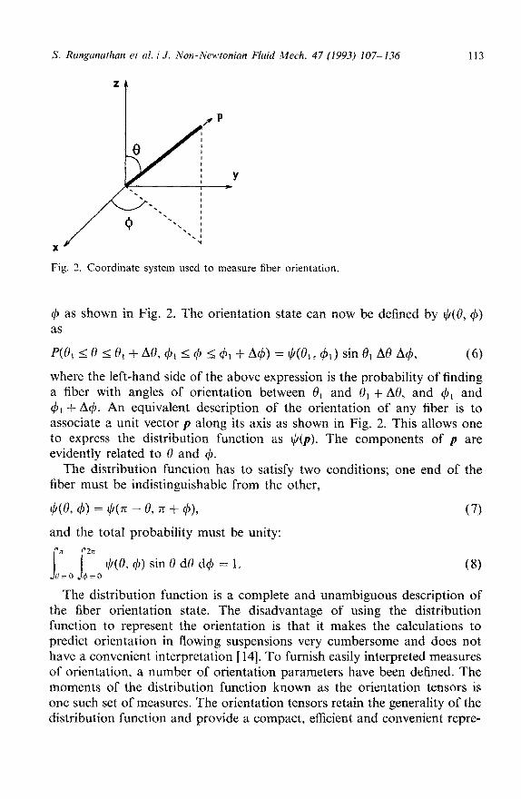
Fig. 2. Coordinate system used to measure fiber orientation.

# as shown in Fig. 2. The orientation state can now be defined by ~~%, 4) as

~(%~<%<%,+A%,~,~~<~,+A~)=11/(%,,~,)sin%,A%A~, (6)

where the left-hand side of the above expression is the probabihty of finding a fiber with angles of orientation between %, and 0, + A%, and 41 and 4, -i- A+. An equivalent description of the orientation of any fiber is to associate a unit vector p along its axis as shown in Fig. 2. This allows one to express the distribution function as r,Q). The components of p are evidently related to % and (13.

The distribution function has to satisfy two conditions; one end of the fiber must be indistinguishable from the other,

$C%l (-b) = ti(n - %, n + (P), (7)

and the total probability must be unity:

tic%. 4) sin%d%d$=i. (8)

The distribution function is a complete and unambiguous description of the fiber orientation state. The disadvantage of using the distribution function to represent the orientation is that it makes the calculations to predict orientation in flowing suspensions very cumbersome and does not have a convenient interpretation [ 141. To furnish easily interpreted measures of orientation, a number of orientation parameters have been defined. The moments of the distribution function known as the orientation tensors is one such set of measures. The orientation tensors retain the generality of the distribution function and provide a compact, efficient and convenient repre-

114 S. ~~t~g~~t~l~n et cri

sentation [ 14J. The components and the fourth-order tensor auk/

41 = (Pip,),

of the second-order orientation tensor a,

are defined as

(9)

(10)

where ( ) represents orientation averaging defined as

(K)=[‘[ g11/(8, c$) sin 0 dQ dqi. (11)

The second- and fourth-order orientation tensors have only 5 and 14 independent components respectively due to the symmetry and normaliza- tion conditions which they satisfy

a,, = aI,, (12a)

arr = 1, (12b)

a,kl = aij& = i&J = a,,,( = . * ., (12c)

a, = @z&k* (124

The orientation state may also be represented by a scalar measure [ 151:

f = 1 - 27 x detla,, 1, (13)

such that f is zero at random orientation and unity at aligned orientations. The conservation equation for the distribution function in the orientation

space,

(14)

describes the transient evolution of the distribution function. The angular velocities s and 4, or fi describing the rotation of the fibers, are given by 1121

d 1 alCi = -&qJ) +$(**p -*j:ppp) -c,qp$-3 (13

where i, is (r,’ - I)/(rz + 1), r, is the equivalent ellipsoidal aspect ratio of the fiber, p is the strain rate tensor and o is the vorticity tensor defined as

au, au, kJ=~+x,’ (16a)

au, au, co,, =- ---, ax, axi ( l6b)

and [j] is the ma~itude of the strain rate tensor. Cr, known as the interaction coefficient, is a phenomenological parameter which measures the

S. R~~ganaf~a~ et af. 1 J. eon-Newtonian Fluid Me&. 47 (1993) 107-136 115

intensity of interactions in a suspension and is a function of the suspension characteristics. Thus, if C, is set to zero, eqn. ( 15) reduces to Jeffery’s [9] equation for the angular motion of an ellipsoid in creeping flow. The predicted steady-state orientation using eqns. (14) and (15), is a strong function of C, when Ci lies between 0( 10-3) and 0( 1). Ranganathan and Advani [ 161 have suggested the use of the average interfiber spacing to estimate the intensity of fiber-fiber interactions in non-dilute suspensions. The results presented in this paper use this approach to determine the value of the interaction coefficient.

The solution of eqn. (14) to obtain the orientation-distribution function is computationally intensive. Moreover, all the information from the orienta- tion distribution is not necessary. It has been shown [ 141 that the nth moment of the distribution function is sufficient to compute an &h-order property of a suspension of axisymmetric particles. Therefore, in order to be able to relate the stresses in a suspension to the strain rates one needs only the fourth-order orientation tensor. The governing equation for the orientation (eqn. (14) may be cast in terms of the fourth-order orientation tensor using eqn. (15) and setting ;1 = 1 [14,17]:

where vij, is the velocity gradient tensor defined as

# = (Vz#. (18)

Equation ( 17) is a set of 81 coupled equations but, as mentioned earlier, due to the symmetry and normalization conditions satisfied by the fourth-order orientation tensor, it reduces to a set of 14 coupled equations. It should be noted that the governing equation for the evolution of the fourth-order tensor contains a sixth-order tensor. Therefore one needs a closure to approximate the sixth-order tensor in terms of lower-order tensors to solve the above system of equations. The hybrid closure [ 1 S] is used to approximate the sixth-order tensor al,kl,,zn in eqn. (I 7) in terms of lower-order tensors.

G2jkhzrz = & (aI&$mn f ar&,&~ -+- ’ ’ ’ 15 tems)

- $(aL$k16rnn f ak16&,,n + ’ ‘45 terms)

+ &(drj&ldnzn + 61k6Jl&,n + ’ ’ . 15 terms) Linear closure [ 171,

(19a)

a,~khn, = %klamn Quadratic closure, t 19b)

Hybrid closure, (19c)

where f is the scalar orientation parameter defined in eqn. (13). The linear closure is exact at random orientation and the quadratic closure is exact at aligned orientations. Since f is zero when the orientation is random and unity at aligned orientation states, it is used as a weighting function to interpolate the closure values for orientations between random and aligned states.

To calculate the flow field of a fiber suspension, one needs to know the stress in the suspension as a function of the deformation rates. This functional relationship is known as a rheological constitutive equa- tion. Such equations have been proposed for fiber suspensions in various concentration regimes. There are several review articles on the subject [ 18-201.

For axis~metri~ particles a general rheological constitutive equation is

14,211

~=P~~A(~PPP):~-~BE~P).~+~.(PP)I+(E~~+C)~, (20)

where P is the pressure, 6 is the unit tensor, r is the stress in the suspension, (. . .) denotes orientation averaging, p is the direction of orientation of a fiber, f is the strain rate tensor, p, is the suspending fluid viscosity, and A, B and C are functions of only the shape of the particles that determine the contribution to the stress field due to the presence of the fibers in the suspension. An attractive feature of this equation is that the effects of the orientation of the particles and their shape on the stresses have been separated. In dilute suspensions of ellipsoidal fibers of large aspect ratio these parameters are given by 1211

A =%C,#Q rf

4[1n 2r, - (3/2)] ’

B = 2~4, 3ln2r,-(11/2)

d 1

(214

(2lb)

c = 2YSAJ’ (21c)

Since B is much smaller in magnitude than A for moderately large rfr it is generally neglected. It has been recently shown [22] that even though eqns. (21) are strictly valid only for dilute suspensions, concentrated suspensions also exhibit the same qualitative stress-total strain behavior as predicted by eqn. (20), using eqn. (21a) to evaluate A.

Dinh and Armstrong [8] derived an expression for the extra stress in a semi-concentrated suspension due to the presence of particles using the approach suggested by Batchelor [3]. They modeled the problem as a test

S. Ranganatha~ et al. /J. No~-~e~~Jton~a~l Fluid Me&. 47 (1993) 101-136 117

fiber in the suspension surrounded by an effective continuum. The result they obtain for the stress tensor in the suspension is

z = p,j[l +.lL id3 12 ln(2h/d) ’ CPPPP)] ’ (22)

where n is the number of fibers per unit volume of the suspension, 1 and d are the length and diameter of the fibers and h is the average distance from the test fiber to its nearest neighbor. It can be shown from eqn. (22) that when the fibers are all aligned along the flow in simple shear they do not contribute to the stress field in the suspension. This is a direct result of using the slender-body approximation, which neglects the finite diameter of the fibers.

Shaqfeh and Fredrickson [23] determined the hydrodynamic stress in a fiber suspension in the dilute and semidilute regimes. They calculated this stress at random and aligned fiber orientation states based on hydrodynamic reflections between the fibers in the suspension. The form of the expression they use for the hydrodynamic stress in the suspension is

z = L4x&PPPP) -sqPP)l : 9 + &?* (2% The isotropic contribution of the particles (the second term in the square brackets in eqn. (23)) to the stresses in the suspension is subtracted from the anisotropic expression for the stress field (first term in the square brackets in eqn. (23)). In an incompressible flow, any isotropic stress is arbitrary and is determined only by the boundary conditions. Therefore, this equation is of exactly the same form as eqn. (20) with B = C = 0 and A = pfr&. For the case of semidilute suspensions Shaqfeh and Fredrickson obtain

8Tcp,n13 1 ilbber = ---y--

ln( I/#,) + In ln( l/#y) - 0.6634 isotropic,

8qusnI’ 1 hber = 3 ln( l/4,) + In ln( l/4,) + 0.1585

aligned,

GW

Since this theory also does not take into account the thickness of the fibers, the shear viscosity is zero when all the fibers are aligned with the flow. The expressions for j&ber may be corrected to account for the finite fiber thickness in an ad hoc manner using the results of Batchelor [24] for dilute suspensions [25]. The expression for ,U fiber given by Batchelor for a dilute suspension with thin long particles is

(25)

where E is l/ln(2rr) andf(E) is the correction factor to account for finite fiber thickness. The function f(e) is given by

f(E) = 1 + 0.646 1 _ 1 .50E + 1 .659C2.

I18 S. Ranganathan et al. 1 J. Non-NebCtonian Fluid Mech. 47 (1993) 107-136

As rf tends to infinity, E tends to 0 logarithmically and Y(E) tends to 1. Due to the logarithmic decay of E, even at a high aspect ratio of 100 the value of f(e) is 1.62. This is significantly larger than 1 and therefore is an appreciable correction for the fiber thickness.

The approaches described above to model the rheology of a suspension have been explicitly developed for macroscopic elongated particles sus- pended in a Newtonian fluid. However, one may also extend rheological models developed for much smaller length scales such as liquid crystals and make the appropriate modifications to account for the changes in the scale. Doraiswamy and Metzner [26] have extended Doi’s [27] rheological consti- tutive equation for liquid crystalline polymers to fiber suspensions. Doi’s theory neglects the contribution of the fiber-fluid friction and internal fluid friction to the total stress in the fluid. This assumption is valid at very small strain rates. Doraiswamy and Metzner[26] recognized that the expression for the stress needed to be modified to account for the higher viscous dissipation at higher shear rates. To accomplish this they added a contribu- tion to the stress in the suspension that is linearly related to the strain rate and the suspending fluid viscosity. The modified equation they obtained was

r=A,h +~r,usj, (27)

where A, is an empirical coefficient, ,LL~ is the relative viscosity of the suspension and

C = v2&d12. (29)

In the above equation V? is a numerical constant, 1 and dare the length and diameter of the fibers and S is the deviatoric second-order orientation tensor related to the second-order orientation tensor a defined earlier by subtrac- tion of the isotropic component,

S=,-;.

Equation (27) is a phenomenological rheological equation where the first term on the right-hand side describes the anisotropy in the suspension and the second term takes into account the internal dissipation in the suspen- sion. It was found [26] that this model fitted the measured stress-strain rate behavior of concentrated suspensions of glass fibers in polypropylene very well over several decades of shear rate. At high shear rates the second term on the right-hand side of eqn. (27) dominates. A comparison of that term with eqn. (20) assuming that the fibers are all aligned with the flow in simple shear, reveals that pr and 1 + 29” are analogous. Table 1 shows a

S. Ranganathan et al. 1 J. Non-Newtonian Fluid Mech. 47 (1993) 107-136 119

TABLE 1

Comparison of experimental data from Becraft [28] and from the approximated dilute rheological equation

0.038 1.1 1.076 0.190 1.4 1.380

comparison of the value of pr obtained by Becraft [28] from his experimental results at high shear rates and the corresponding values of 1 + 24”. It is seen that even though the analogy between ,u~ and 1 + 24” is strictly valid only for dilute suspensions, it seems to model the behavior of even concentrated suspensions adequately.

The primary difference between the models reviewed above is that the Shaqfeh-Fredrickson and Dinh-Armstrong models, which are based on theoretical suspension mechanics, exhibit a linear dependence of the stress field in the suspension on the strain rate, related through the orientation state. However, the Doraiswamy-Metiner model, which is phenomenological, gives the stress in the suspension as separate functions of the orientation state and strain rate. In this work, we do not use the Doraiswamy-Metzner model, as in their approach the constant A, must be first determined, which requires experimental data. Instead, we use the Shaqfeh-Fredrickson approach, introducing the corrections for the finite diameter of the fibers to represent the rheology of the suspension. The Dinh-Armstrong model which is of the same form can also be used. The primary difference between these two models is the coefficient multiplying the fourth-order orientation tensor in the rheological equation.

In the next section, we delineate a general procedure to solve the flow and fiber orientation in an axisymmetric configuration and specialize it to a radial flow case. The advantage ofthis configuration is that the flow is two dimensional but the orientation state is three dimensional. This allows us to investigate the effect of three-dimensional orientation on the kinematics of a simple flow. This will lead to a better understanding of the nature of the coupling between the flow and the fiber orientation. In this work we also analyze the effect of the presence of the particles on the developing length for the flow field. This length characterizes the significance of the effect of the fibers on the flow field.

4. Coupled solution for fiber orientation and flow

If the fluid under consideration is highly viscous, one can neglect the inertia and body-force terms in the momentum equation, i.e. the Reynolds

110 S. ~angunath~~l et rd. 1 J. _~o~-Ne~stonian Fluid Me&. 47 (1993) 107-136

number is very small. The steady momentum equations for axisymmetric flow under this assumption are

where Y and s are the radial and gapwise coordinates respectively. Cross- differentiating eqns. (31a) and (31 b) to eliminate the pressure from them yields

The stresses z in eqn. (32) can be expressed in terms of the fiber orientation, fiber volume fraction, fiber aspect ratio and the strain rates by using a modified form of the rheological equation given by Shaqfeh and Fredrickson 1231:

r = /&J(E) [ (PPPP > - 5 6 OrP > 1 : li + Ps ( 1 f h)?. (331

The correction factor f(~) given by eqn. (26) is introduced to correct the expression for ,&ber for the finite fiber thickness and the term 2~ is added to the last term to account for the contribution of the fibers to the stresses even at an aligned orientation state. Both these corrections are made by drawing parallels with the dilute suspension theory [21,24]. The justification for using these dilute suspension corrections for non-dilute suspensions has been discussed earlier.

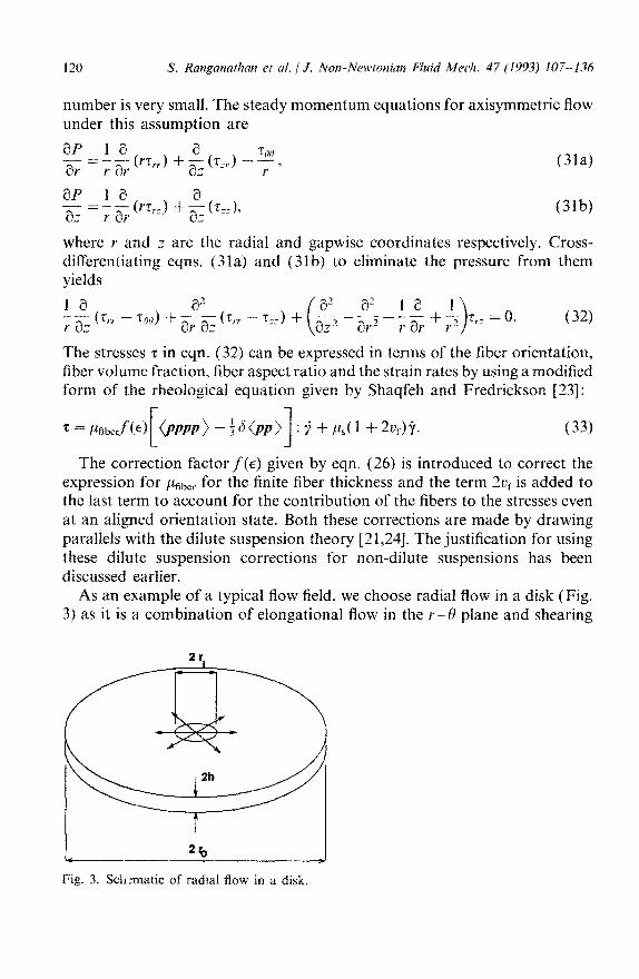
As an example of a typical flow field, we choose radiaf. flow in a disk (Fig. 3) as it is a combination of elongational flow in the r-0 plane and shearing

Fig. 3. Sch:matic of radial flow in a disk.

flow in the T--Z plane. An interesting aspect of this flow geometry is that the region near the boundaries are shear dominant (v/Z > 50) and the region near the midplane of the gap is elongation dominant (y/i: < 10). The shear-dominant region increases in size as compared to the elongation- dominant region as the radial distance increases. This leads to a change in the characteristic behavior of the fiber orientation through the gap and with the radial location. In the intermediate or transition region in the gap we expect to see the combined effect of shear and elongation.

The governing equations are now non-dimensionalized and specialized for the particular problem under consideration. The r and I’ coordinates are non-dimensionalized with the characteristic length in each direction, R and L, respectively,

5=;, ( 344

(34b)

The velocity in the r direction is non-dimensionalized with the uniform inlet velocity U.

t,+ =:!!!z i u’ (3W

where V, is the characteristic velocity in the z direction. The continuity equation given below,

(36)

provides the right scaling for the choice of vZC as U(L/R). Therefore, the continuity equation in non-dimensional form reduces to

(37)

The stream function is non-dimensionalized with ULR, and the relationship between the velocity and the stream function in non-dimensional form is

The strain rates are non-dimensionalized with U/R to give

(3W

t 39b)

(39d)

The rheological equation expressed in terms of the non-dimensional strain rates with the stresses non-dimensionalized by psUIR is given by

(40)

and the non-dimensional form of the equation of motion (32) may be written as

(41)

For radial flow in a disk geometry, the relevant length scales R and L, are, u, the radius of the disk and h the half thickness of the disk respectively;

R ==r,, WW

i-2 =h. (42b)

If one knows the orientation state in a domain, eqn. (40) can be used to express the components of the stress tensor in terms of the velocity gradients and to solve eqn. (41) subject to boundary conditions to calculate the flow field. However, it is more efficient to express eqn, (41) in terms of the stream function. This results in a fourth-order partial differential equation for Y in the space variables r and 2. Therefore, we need four boundary conditions in each direction to find the solution for Y and in turn calculate the velocity field (eqn. (38)).

Equation (17) is used to calculate the orientation evolution and the indices in that equation take on the values 1, 2 and 3 that correspond to the Y, 8 and 2 directions respectively. Equation ( 17) can be solved as an initial value problem knowing the velocity field in the domain. The only initial condition needed is the initial orientation state. We adopt a Lagrangian

S. Ranganathan et al. 1 J. Non-Newtonian Fluid Mech. 47 (1993) 107-136 123

No Slip

Fig. 4. Boundary conditions for the radial flow in a disk.

viewpoint and follow the history of the orientation state from the initial point to any point of interest in the computational domain, using a coordinate system fixed to the particles. Therefore the convective part of the material derivative in eqn. ( 17) drops out. Equation (41) can now be solved along with the system of eqns. (17), using the relationships in eqn. (40) to couple them.

The geometry of the disk is discretized into a finite difference grid of rectangular elements. The boundary conditions applied for the flow are shown in Fig. 4. Since the flow and orientation should be symmetric about the mid-plane of the gap, the solution is carried out only in one half of the domain. The inlet flow boundary condition may be chosen as either a uniform profile or a fully developed parabolic profile. Preliminary calcula- tions were performed with both these choices and it was found that due to the nature of the flow field rearrangement, the orientation calculations for the latter inlet condition took much longer. Therefore the results presented in this paper are with a uniform radial velocity through the gap at the inlet. There is no flow, parallel or perpendicular, at the wall. At the midplane a symmetry boundary condition is specified and at the exit the velocity through the gap and its derivative with respect to the radial direction are specified to be zero. These can be summarized as

v, = u, U,=O at Y=Yi, (43a)

av, - 0

ar ’ v,=O at r=rO, (43b)

v, =o, v, = 0 at z = h, (43c)

(43d)

In terms of the non-dimensional quantities defined earlier, these can be rewritten as

YJ+ = -41% NJ+ -=0 at l=[,,

X (44a)

124 S. Rangarzathan et al. 1 J. Non-Newtoniuu Fluid Me& 47 (1993) 107-136

aY!+ - =o,

iPP+

at -=0 at<=l,

a<?

ay+ =. ay+ -=0 atq=l,

atj ’ a;

( 44b)

(44c)

aw - = 0,

a\y+

a+ -=0 atq=O.

at (44d)

The orientation evolution is solved as an initial value problem, with the option to specify any orientation state at the inlet. The results presented in this paper have been obtained using an isotropic initial orientation, unless otherwise indicated. However, calculations were also performed with a perfectly aligned orientation state in the thickness direction to explore the influence of the inlet-orientation condition on the behavior of fiber suspen- sions. The starting point of streamlines passing through each node in the computational domain is identified from the flow field results. Since the initial orientation is known, the set of 14 coupled non-linear evolution equations ( 17) may be integrated along the streamlines to obtain the orientation states at the various nodes in the interior of the domain. A schematic representation of this is shown in Fig. 5. The strain rate and velocity values along the streamlines are obtained by linearly interpolating their values from the neighboring nodes. The average velocity and the effective length L, along a streamline between two adjacent points of calculation, represented by black dots in Fig. 5, are used to estimate At, the time taken by the orientation state to convect with the fluid from one position to the next. The set of evolution eqn. ( 17) representing the orientation state can now be integrated over this period of time At to obtain the change in orientation. The method described above can be used every- where in the computational domain except at the wall where the velocity is

Inlet

Point of interest

- Finite Grid

-0- Streamline

Fig. 5. Integration of orientation tensor values along streamlines.

125

In&l guess) / I

I Update rheological

---+ COupled Solution

----* Decoupled Solution

Fig. 6. ~ethodolo~ for solution of Row and orientation of a fiber suspension.

imposed to be zero. Therefore, we need to make an assumption about the orientation state along the wall. The orientation at the wall is assumed to reach an aligned state instantaneously. This assumption is justified due to the high shear and small velocities in the proximity of the wall. It may be argued that the fibers at the wall should take on the steady orientation rather than the aligned orientation state, but this would be the case only if the wall does not affect the angular motion of the fibers. Since we do not explicitly account for any fiber-wall interactions, this assumption, in a way, models the fiber-wall interactions.

The solution methodology for the flow and fiber orientation is shown in Fig. 6. The decoupled approach assumes that the flow field is unaffected by the presence of the fibers. In this case the flow field is calculated based on the rheology of the suspending fluid, the geometry of the flow field and the boundary conditions. Subsequently, the orientation evolution equations are integrated along the str~mlines of the flow field to obtain the orientation state at the various locations in the flow field. IIowever, if the effect of the

presence of the fibers on the flow field is not ignored, the governing equations, (32) and ( 17) become coupled. The orientation states cannot be calculated due to the lack of knowledge of the streamlines and the flow field cannot be calculated due to the lack of knowledge of the rheological properties of the suspension at various locations in the domain of interest. Hence, we resort to an iterative solution technique. The Newtonian flow solution is obtained first by neglecting the presence of the fibers. The orientation state is calculated based on this flow feld. Using these orientation states, the rheological properties of the suspension are evaluated at all the nodal points in the computational domain. The flow field is recalculated with the newly estimated rheological properties. This procedure is repeated until conver- gence is obtained in the predicted flow field and the fiber orientation state. For simulations of flow and orientation for high fiber volume fraction suspensions, the initial guess of velocity field used was the one obtained from the steady solution of the lower volume fraction simulations instead of the Newtonian solution. This technique was found to reduce the number of iterations required for the convergence of the results.

5. Results and discussion

In this section, some of the results of the various presented. The predicted radial velocity results will be a modified dimensionless radial velocity defined as

uv,(r, I)

cases studied will be presented in terms of

(45)

where r, is the radial position of the inlet and u,., is the inlet velocity. This definition arises from the fact that, in a radial flow configuration, ru, is a measure of the flow rate at any radial position. Even though the fourth- order orientation tensor components were calculated, the orientation results are presented in terms of the second-order orientation tensor components for the sake of compactness. The second-order orientation tensor components are obtained from the fourth-order tensor components using eqn. (12d).

The values of the interaction coefficient used in the calculations were determined using eqn. (46) [ 161 and a value of 10 .. ’ for K

0 -I

C,=K 2 ) (46)

where a, is the average inter-fiber spacing, d is the diameter of an individual fiber and K is a constant of proportionality determined experimentally. All the simulation results presented here correspond to h = 0.05, I”, = 0.05, and I’~ = 1.05. As ct,/d changes with the orientation state, C, also varies with the orientation.

S. Ra~~anathan et al. 1 J. bob-Newtonian Fluid Mech. 47 (1993) I&-136 127

0.14

0.12

0.1

1 0.08

i 0.06

0.04

0.02

0

I I

NewtodrnSdution - Numaiul2lXll noda l

Numaicd 21X21 noda +

0 0.2 0.4 0.6 0.8 Hsioln

Fig. 7. Comparison of steady velocity profile obtained from the numerical simulation with the Newtonian solution.

The steady results from the numerical scheme for a Newtonian fluid were first compared to the results for the fully developed velocity field which can be obtained analytically (Fig. 7). This figure shows the radial velocity profile from the numerical simulation at a radial distance of 20h from the injection point. It is seen that there is good agreement between the two, and 21 nodes through the thickness gives adequate accuracy in the numerical results for the Newtonian case, The convergence of the velocity predictions of the coupled solution for a 0.01 fiber volume fraction suspension is shown in Fig. 8. It is seen that the difference in the predictions between 21 and 31 nodes through the thickness is very small. However, the computation time for 31 nodes through the thickness was much greater than that for 21 nodes. The suspension close to the wall undergoes a higher total shear for the same radial distance than the suspension close to the centerline. Since the time step for the integration of the orientation equations is governed by the maximum total shear per integration step, the orientation calculations in the region close to the wall take much longer than in the region away from the wall. In the interest of accuracy and practical computation times, 21 nodes through the thickness and 61 nodes in the radial direction were used for all the results presented in this paper.

0 0.1 0.2 0.3 0.4 0.5 0.6 0.7 0.8 0.9 1 Dimensionless radial location

Fig. 8. Modified dimensionless centerline radial velocity with I I, 21 and 31 nodes through the gap obtained by the coupled solution for a 0.01 fiber volume fraction suspension.

The streamlines for the numerically calculated Newtonian flow field are

shown in Fig. 9(a). It is seen that most of the rearrangement of the

streamlines takes place very close to the inlet. The initial flow from the regions near the wall where the fluid decelerates to the region near the midplane where the fluid accelerates is indicated by the streamlines tending towards the midplane.

The orientation state in the disk calculated using the Newtonian stream- lines and a fiber volume fraction of 0.01 and fiber aspect ratio of SO is shown in Fig. 9(b). The value of the interaction coefficient for this case varied from 0.01 at a random orientation state to 0.002 at an aligned orientation state. The orientation state is represented by ellipses whose major and minor axes are oriented in the principal directions of orientation, The length of the major and minor axes of the ellipse indicate the relative magnitudes of the principal strength of orientation in the respective direc- tions. For example, a line represents perfect alignment in the direction it lies in, a circle represents random in-plane orientation and a circle with radius close to zero represents perfect alignment out of plane. It is seen that the fibers near the midplane orient themselves in the stretching direction, perpendicular to the plane of the paper. The fibers in the region near the wall tend to align along the flow direction due to the high shear rates they

129

(3)

0 0 0

0

0

0

0

0

0

(q3)

Centerline

Wall

- - - _I - _ _ - ---..- ---.._ A ---_ A \ --.-_ ---_

. - ---.. - - - ---.... . . - ---.._ - - --

- - I -----.

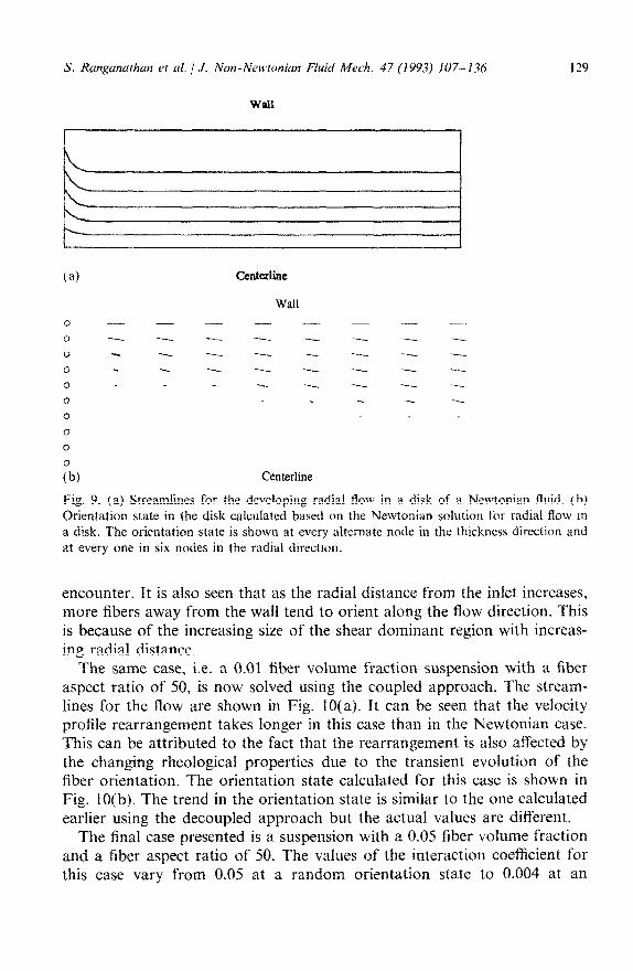
Fig. 9. (a) Streamlines for the developing radial flow in a disk of a Newtonian fluid. (b) Orientation state in the disk calculated based on the Newtonjan solution for radial flow m a disk. The orientation state is shown at every alternate node in the thickness direction and at every one in six nodes in the radial directlon.

encounter. It is also seen that as the radial distance from the inlet increases, more fibers away from the wall tend to orient along the flow direction. This is because of the increasing size of the shear dominant region with increas- ing radial distance.

The same case, i.e. a 0.01 fiber volume fraction suspension with a fiber aspect ratio of 50, is now solved using the coupled approach. The stream- lines for the flow are shown in Fig. IO(a). It can be seen that the vetocity profile rearrangement takes longer in this case than in the Newtonian case. This can be attributed to the fact that the rearrangement is also affected by the changing rheologi~ai properties due to the transient evolution of the fiber orientation. The orientation state calculated for this case is shown in Fig. IO(b). The trend in the orientation state is similar to the one calculated earlier using the decoupled approach but the actual values are different.

The final case presented is a suspension with a 0.05 fiber volume fraction and a fiber aspect ratio of 50. The values of the interaction coe~~ient for this case vary from 0.05 at a random orientation state to 0.004 at an

o--------

0 . - ---... ---._ _ - - -

0 . - -_ -_ - - -

0 . -4 - - -m..... -

0 --... . . - -

0 .

0

0

0

0

(b) Centerline

Fig. 10. (a) Streamlines for the developing radial flow in a disk of a fiber suspension of volume fraction 0.01 and fiber aspect ratio of 50. (b) Orientation state for radial flow in a disk of a suspension of volume fraction 0.01 and fiber aspect ratio 50. The orientation state is shown at every alternate node in the thickness direction and at every one in six nodes in the radiaf direction.

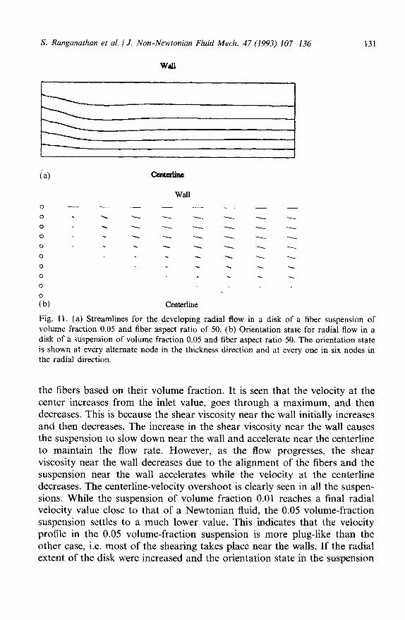
aligned orientation state. The streamlines and the orientation state are shown in Fig. 1 l(a) and 1 l(b). It is seen from this set of figures that a trend of deviation from the Newtonian prediction similar to what was observed at a fiber volume fraction of 0.01 is also observed at a volume fraction of 0.05 but in a conclusively noticeable manner. Qualitatively this is to be expected, since, as the volume fraction increases, the rheology of the suspension deviates more from that of the suspending fluid.

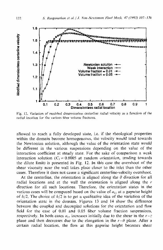
The results of velocity and orientation presented above are consolidated in the following manner. The modified dimensionless centerline radial velocity is shown in Fig. 12. From this figure it is seen that while, in the Newtonian case, the flow develops fully within the first few gap heights of the inlet, it takes longer in suspensions with non-zero fiber volume fraction. This is because the presence of the fibers affects the rheology of the suspension. Among the suspensions there is a difference in the developing behavior of the flow due to the difference in the contribution to the stress by

S. Ra~gu~~thun et ai. j J. ~on-Ne~to~i~n Fluid Mech. 47 (i993) 107-136 131

WJlll

ia) caltuiinc

Wall o-----..-._______ 0 . . - . - . -_ -...._

0 . . . . . - -

0 . -_ . - - -

0 - . . .

0 . . .

0

0

0

0

(b) Centerline

Fig. 11. (a) Streamlines for the developing radial flow in a disk of a fiber suspension of volume fraction 0.05 and fiber aspect ratio of 50. (b) Orientation state for radial flow in a disk of a suspension of volume fraction 0.05 and fiber aspect ratio 50. The orientation state is shown at every alternate node in the thickness direction and at every one in six nodes in the radial direction.

the fibers based on their volume fraction. It is seen that the velocity at the center increases from the inlet value, goes through a maximum, and then decreases. This is because the shear viscosity near the wall initially increases and then decreases. The increase in the shear viscosity near the wall causes the suspension to slow down near the wall and accelerate near the centerline to maintain the flow rate. However, as the flow progresses, the shear viscosity near the wall decreases due to the alignment of the fibers and the suspension near the wall accelerates while the velocity at the centerline decreases. The centerline-velocity overshoot is clearly seen in all the suspen- sions. While the suspension of volume fraction 0.01 reaches a final radial velocity value close to that of a Newtonian fluid, the 0.05 volume-fraction suspension settles to a much lower value. This indicates that the velocity profile in the 0.05 volume-fraction suspension is more plug-like than the other case, i.e. most of the shearing takes place near the walls. If the radial extent of the disk were increased and the o~entation state in the suspension

Ne~onlan solutkrn -+- Weak interaction --

Volume fraction I 0.01 +--- Volume fraction = 0.05 --

0.1 0.2 0.3 06 ~irn~~~“~~~~ radial locat%

0.8 0.9 1

Fig. 12. Variation of modified dimensionless centerline radial velocity as a function of the

radial location for the various fiber volume fractions.

allowed to reach a fully developed state, i.e. if the rheo~ogical properties within the domain become homogeneous, the velocity would tend towards the Newtonian solution, although the value of the orientation state wouId be different in the various suspensions depending on the value of the interaction coe~cient at steady state. For the sake of comparison a weak interaction solution (C, = 0.0005 at random orientation, tending towards the dilute limit) is presented in Fig. 12. In this case the overshoot of the shear viscosity near the wall takes place closer to the inlet than the other cases. Therefore it does not cause a significant centerline-velocity overshoot,

At the centerline, the orientation is aligned along the 0 direction for all radial locations and at the wall the orientation is aligned along the f direction for all such locations. Therefore, the orientation states in the various cases will be compared based on the value of LI~ I at a gapwise height of h/2. The choice of /z/2 is to get a qualitative idea of the variation of the orientation state in the domain. Figures 13 and 14 show the difference between the coupled and decoupled solutions for the orientation and flow field for the case of 0.01 and 0.05 fiber volume fraction suspensions, respectively. In both cases a,, increases initially due to the shear in the r-z plane and then decreases due to the elongation in the r-B plane. After a certain radial location, the Aow at this gapwise height becomes shear

S. Ranganutkan et al. 1 J. Non-Newtoman Fluid Meek. 47 (1993) 107- 136

0.7

0.6

0.5

0.4

0.3

0.2

0.1

0

Decoupled solution - Coupled solution -+---

I I 1 I I I 1 I I 0.1 0.2 0.3 0.4 0.5 0.6 0.7 0.6 0.9 1

Dimensionless radial location

Fig. 13. Comparison of coupled and decoupled solutions for the orientation tensor compo- nent a,, at a gapwise height of /z/2; fiber volume fraction = 0.01.

0.9

0.8

f 0.7

f! i OX

8 0.5

E 0.4 w C

.$ 0.3 (0

g 0.2

0.1

0

- Coupled solution +- Iecoupled solution -+---

0.1 0.2 0.3 Dimension&~ 0.4 rad~l%cat% 0.8 0.9 i

Fig. 14. Comparison of coupled and decoupled solutions for the orientation tensor compo- nent a,, at a gapwise height of h/2; fiber volume fraction = 0.05.

dominant and a,, increases monotonically beyond it. The difference between the predicted orientation results using the coupled and decoupled approaches is apparent in each case. This difference in orientation states also manifests itself in the form of different velocity field solutions when using the coupled and decoupled approaches. It should be noted that the orientation in both these cases would reach a steady-state value at a larger radial distance than shown in Figs. 13 and 14.

The boundary condition applied at the exit of the fiow domain, eqn. (43), is strictly valid only beyond a radial distance sufficient for the steady orientation to have been reached through the gap. However, in our simulations this boundary condition was applied at a distance of 20h from the inlet to reduce the computational time. As a test case, the simulation was performed for the 0.05 volume fraction case up to a radial distance of 100/z. The predicted velocity field in this case showed the same trend as the simulation where the exit boundary condition was applied at 2012. Another point worth noting is that for a value of the interaction coefficient between O( 10e3) and 0( 1) the strength of orientation would be different depending on the actual numerical value of C,. However, we expect the overall qualitative behavior of the predicted velocity and orientation state to remain essentially unaltered.

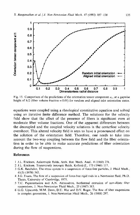
If the inlet flow boundary condition was specified as parabolic, the developing flow field would be quantitatively different. However, the orien- tation state would be qualitatively similar because the flow field is still shear dominant near the wall and elongation dominant near the centerline. We also changed the inlet orientation condition to perfectly aligned in the gapwise direction, based on the knowledge that the fibers settle in this o~entation state as they exit the vertical pipe prior to entering the disk. The maximum difference between the orientation predictions using two different inlet conditions is expected at a gapwise location halfway between the centerline and the wall as the flow is neither shear nor elongation dominant in this region. Therefore, the predicted values of a,, at this gapwise location, using isotropic and aligned initial orientation states are shown in Fig. 15 as a function of the radial location. The difference between the two predictions demonstrates the importance of the inlet orientation condition, at least in the region away from the waI1 and the centerline.

Finally, the results of our coupled model could not be compared to an ‘aligned-rod’ approximation prediction. This is because our flow configuration does not satisfy the stability condition given by Lipscomb et al. [6] for the aligned-rod to be an equilibrium solution.

6. Summary

The flow and orientation of a fiber suspension were studied in a radial flow geometry. The momentum equations and the orientation evolution

S. Ranganathan et al. /J. Non-Newtonian Fluid Mech. 47 (1993) 107-136 135

1 I I I I I 1 I I 1

0.9 - __++_++++++++++++-

Random initial orientation - - Aligned initial orientation -+--

0.1 0.2 0.3 0.4 0.5 0.6 0.7 0.6 0.9 1 Dimensionless radial distance

Fig. 15. Comparison of the predictions of the orientation tensor component a,, at a gapwise height of h/2 (fiber volume fraction = 0.01) for random and aligned inlet orientation states.

equations were coupled using a rheological constitutive equation and solved using an iterative finite difference method. The solutions for the velocity field show that the effect of the presence of fibers is significant even at moderate fiber volume fractions. One of the apparent differences between the decoupled and the coupled velocity solutions is the centerline velocity overshoot. This altered velocity field is seen to have a pronounced effect on the solution of the orientation field. Therefore, one needs to take into account the two-way coupling between the flow field and the fiber orienta- tion in order to be able to make accurate predictions of fiber orientation during the flow of suspensions.

References

J.L. Ericksen, Anisotropic fluids, Arch. Rat. Mech. Anal., 4 (1960) 231. J.L. Ericksen, Transversely isotropic fluids, Kolloid-Z., 173 (1960) 117. G.K. Batchelor, The stress system in a suspension of force-free particles, J. Fluid Mech., 41(3) (1970) 545. J.G. Evans, The flow of a suspension of force-free rigid rods in a Newtonian fluid, Ph.D. Thesis, University of Cambridge, 1975. T.C. Papanastasiou and A.N. Alexandrou, Isothermal extrusion of non-dilute fiber suspensions, J. Non-Newtonian Fluid Mech.. 25 (1987) 313. G.G. Lipscomb, M.M. Denn. D.U. Hur and D.V. Boger, The flow of fiber suspensions in complex geometries, J. Non-Newtonian Fluid Mech., 26 (1988) 297.

7 CL. Tucker, Flow regimes for fiber suspensrons in narrow gaps. J. Non-Newtonian Fluid

Mech., 39 (1991) 239. S S.M. Dinh and R.C. Armstrong, A rheologrcal equation of state for semiconcentrated

suspensions, J. Rheol.. 2S( 3) (1984) 207. 9 C.B. Jeffery, The motion of ellipsoidal particles immersed in a viscous fluid, Proc. R. SOC.

London, Ser. A, 102 (1923) 161. 10 T.C. Papanastasiou, LE. Striven and C.W. Mackosko, Finite-element method for liquids

with memory, J. Non-Newtonian Fluid Mech., 22 (1987) 271. I1 M.C. Altan, S.I. Guceri and R.B. Pipes, Anisotropic channel flow of fiber suspensions, J.

Non-Newtonian Fluid Mech., 42 ( 1992) 65. 12 F.P. Folgar and CL. Tucker, Orientation behavior of fibers in concentrated suspensions,

J. Reinf. Plast. Compos., 3 ( 1984) 98. I3 S. Ranganathan and S.G. Advani, Characterization of orientation clustering in short

fiber composites, J. Polym. Sci. Polym. Phys. Ed., 28 (1990) 2651. 14 S.G. Advani and C.L. Tucker, The use of tensors to describe and predict fiber orientation

in short fiber composites, J. Rheol., 31 (1987) 751. 1.5 S.G. Advani and C.L. Tucker. Closure appro~inlat~ons for three-d~meIlsiona1 structure

tensors. J. Rheol.. 34(3) ( 1990) 367. I6 S. Ranganathan and S.G. Advani, Fiber-fiber interactions in homogeneous flows of

nondilute suspensions, J. Rheol., 35(S) (1991) 1499. 17 M.C. Altan. Rheology of fiber suspensions and fiber or~entafion analysrs in flow

processes, Ph.D. Thesis. University of Delaware, 1989. I8 A.B. Metzner, Rheology of suspensions m polymeric liquids. J. Rheol., 29 (1985) 739 19 M.R. Kamal and A.T. Mutel, Rheological properties of suspensions in Newtonian and

Non-Newtonian fluids, J. Polym. Eng., 5(4) (1985) 293. 20 E. Ganani and R.L. Powell, Suspensions of rod-like particles: literature review and data

correlations, J. Compos. Mater., I9 ( 1985) 194. 21 E.J. Hinch and L.G. Leal, The effect of brownian motion on the rheological properties

of a suspension of non-spherical particles. J. Fluid Mech., 52(4) (1972) 683. 22 G. Ausias, J.F. Agassant, M. Vincent, PG. Lafleur, P.A. Lavoie and P.J. Carreau,

Rheology of short-glass-fiber-reinforced poiypropyJene, J. Rheol,, 3614) ( 1992) 525. 23 E.S.G. Shaqfeh and G.H. Fredrickson, The hydrodynamic stress in a suspension of rods,

Phys. Fluids A, 2 (1990) 7. 24 G.K. Batchelor, Slender-body theory for particles of arbitrary cross-section in Stokes

flow, J. Fluid Mech., 44(3) (1970) 419. 25 C.A. Stover, The dynamics of fibers suspended in shear flows, Ph.D. Thesis, Cornell

University, 1991. 26 D. Dora~swamy and A.B. Metzner, The rheology of polymerrc liquid crystals, Technical

Report CCM-86-12. Center for Composite Materials. University of Deiaware, 1986. 27 M. Doi, Molecular dynamics and rheological properties of concentrated solutions of

rod-like polymers in isotropic and liquid crystalline phases, J. Polym. Sci. Polym. Phys. Ed., 19 (1981) 229.

28 M.L. Becraft, The rheology of concentrated fiber suspensrons, Ph.D. Thesis, Umversity of Delaware, 1988.