variational solution of axisymmetric fluid flow in tubes with surface solidification

Final year project dealing with

obtaining the approximate analytical

solution to the nonlinear, two-

dimensional free-boundary problem of

axisymmetric heat conduction with

internal surface solidification in the

inlet regions of the tube under the

guidance of

Variational

Solution of

Axisymmetric Fluid

Flow in Tubes with

Surface

Solidification

Variational Solution of Axisymmetric Fluid Flow in Tubes with Surface Solidification Submitted by: Santosh Kumar Verma 07/ME/52 Department of Mechanical Engg. National Institute of Technology Durgapur India

Dr. A K PRAMANICK

Variational Solution of Axisymmetric Fluid Flow in Tubes with Surface Solidification

1

4

Boundary Conditions………………………………………………………………………….…16 Continuity Equation……………………………………………………………………………..17

Basic principle………………………………………………………………………….17

Application to the problem……………………………………………………...18 Equation of motion………………………………………………………………………….…..19

Basic principle………………………………………………………………………….19

Application to the problem……………………………………………………...21 Energy equation in solid phase……………………………………………………………..22

Basic principle………………………………………………………………………….22

Application to the problem………………………………………………………23 Energy equation in liquid phase……………………………………………………………24

Basic principle………………………………………………………………………….24

Application to the problem………………………………………………………25

NOMENCLATURE

ACKNOWLEDGEMENT

SPECIAL FEATURES

CERTIFICATE

Title Page

ABSTRACT

INTRODUCTION

PREVIOUS WORKS

ANALYSIS

5

6

8

9

10

11

13


2

Variational energy equation, liquid region……………………………………………….26

Variational energy equation, solid region…………………………………………………30

Basic principle………………………………………………………………………………………….32

Application to the problem……………………………………………………………………..33

First solution……………………………………………………………………………….33

Second solution…………………………………………………………………………..35

Third solution………………………………………………………………………………36

Integral energy equation, liquid region…………………………………………………….40

Basic principle………………………………………………………………………………………….42

Application to the problem……………………………………………………………………..43

First solution……………………………………………………………………………….43

Second solution…………………………………………………………………………..45

Comparison of methods predicting the solidification history of water………47 Comparison of methods for predicting the axial distribution of ice layers…49 Comparison of limiting transient solutions with available non-flow data….51 Comparison of limiting solution with available steady state data…………….53 Comparison of variational solution based on different profiles………………..55

Cylindrical coordinates…………………………………………………………………………….57 Euler’s equation for variational calculus…………………………………………………..59

VARIATIONAL SOLUTION BASED ON PROFILE (V)

STEADY STATE SOLUTION (V)

SHORT TIME SOLUTION (V)

VARIATIONAL SOLUTION BASED NUSSELT NUMBER AND PROFILE (VN)

STEADY STATE SOLUTION (VN)

GRAPHICAL INTERPRETATION

APPENDIX

LIMITATIONS

26

32

38

42

46

57

60


3

FUTURE SCOPE

REFERENCES

60

61


4

NATIONAL INSTITUTE OF TECHNOLOGY DURGAPUR

WEST BENGAL (INDIA) 713209

This is to certify that the project work titled “Variational Solution of

Axisymmetric Fluid Flow in Tubes with Surface Solidification” is a

bonafide work done by Santosh Kumar Verma, Roll no 07/ME/52, of

Mechanical Engineering Department of National Institute of

Technology Durgapur under the curriculum of the institute for the final

year students during 7th and 8th semester.

Dr. Achintya Kumar Pramanick

Professor

Department of Mechanical Engineering

Place: Signature of the Guide:

Date:

https://encrypted.google.com/url?sa=t&source=web&cd=3&ved=0CCEQFjAC&url=http%3A%2F%2Fwww.nitdgp.ac.in%2Fme%2Fprofiles%2Ffaculty%2Fakumarpramanick.html&ei=O0WATdOpLIbLrQeR-NimBw&usg=AFQjCNGx_JnRoiNTwN0vm16fIvXdN5uliQ&sig2=lhZ6YOhcb5gtimw4Bg9EjQ


5

I, Santosh Kumar Verma, a student of National Institute of Technology

Durgapur, have done this project for partial fulfilment of my B.Tech. graduation

degree at the institute under the curriculum programme for B.Tech. final year

students of Mechanical Engineering.

I am indebted towards Dr. Achintya Kumar Pramanick, my project guide,

for providing me with this opportunity to undertake the project, and to work

under his profound guidance and support.

I take this opportunity to thank Mr. Pinaki Pal and Dr. Seema Mondal

Sarkar from the Department of Mathematics for endowing me with their

knowledgeable help to undertake this project & for their kind cooperation.

I would like to take this opportunity to thank all my friends for being so

kind and cooperative at each and every step.

A special thanks to the management of National Institute of Technology

Durgapur for being supportive during this whole year in order to complete the

project report.

Santosh Kumar Verma March 2011, India


6

Tube radius Constants used in the definition of Nusselt Number Generalized coordinate in the solid region Specific heat Generalized coordinate in the liquid region Heat transfer coefficient Functional integral Thermal conductivity Thermal conductivity ratio = Dimensionless length of tube = Latent heat Lagrangian density N Nusselt number = Pressure Dimensionless pressure =

Peclet number = Prandtl number = Radial coordinate Interface position Dimensionless radial coordinate = Dimensionless interface position = Reynolds number = / Thickness of solid phase = Dimensionless thickness of solid phase = Time coordinate Temperature Mean inlet velocity Velocity Dimensionless velocity Hyper volume in the n-dimensionless space Set of coordinates in the n-dimensional space Axial coordinate

Notations


7

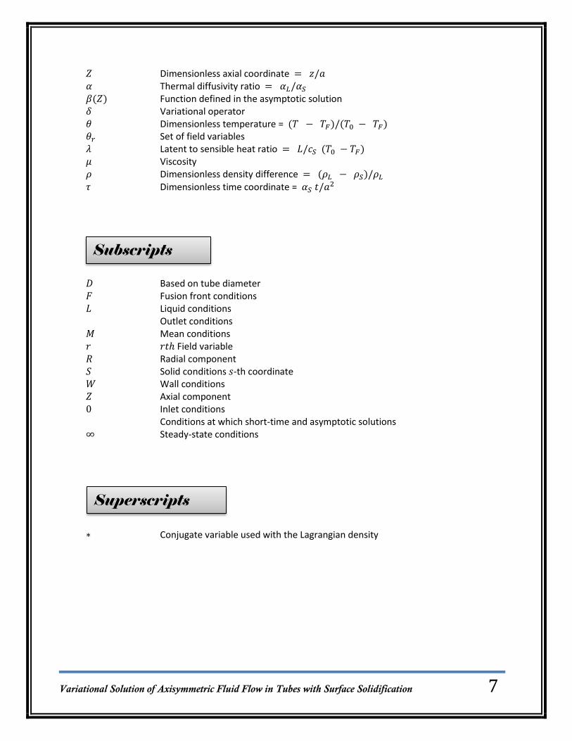
Dimensionless axial coordinate Thermal diffusivity ratio Function defined in the asymptotic solution Variational operator Dimensionless temperature = Set of field variables Latent to sensible heat ratio Viscosity Dimensionless density difference Dimensionless time coordinate =

Based on tube diameter Fusion front conditions Liquid conditions Outlet conditions Mean conditions Field variable Radial component Solid conditions -th coordinate Wall conditions Axial component Inlet conditions Conditions at which short-time and asymptotic solutions Steady-state conditions

Conjugate variable used with the Lagrangian density

Subscripts

Superscripts s


8

Additional information that has been used in different

sections of this paper for different purposes have been

placed in the Solid Box

The solutions obtained by solving different characteristic

equations for the purpose of comparison with the solutions

obtained by the author have been put in a Dash Box

Original solutions to the problems that were obtained by

the author and have been included in the research paper

are boxed in the Long Dash Dot Box


9

The problem of axisymmetric heat conduction with internal surface solidification in

the regions of tube is discussed. An approximate analytical solution is presented to this

nonlinear, two dimensional free boundary problem. The analysis employs a variational

technique which extends the Lagrangian formalism to treat the internal flow, two-

dimensional moving-interface problems. The solution is expressed in the terms of the short-

time and steady-state components. Two forms of the variational solution are presented. One

has limited validity in the entrance region of the tube, and the other, while less general , is

more accurate.


10

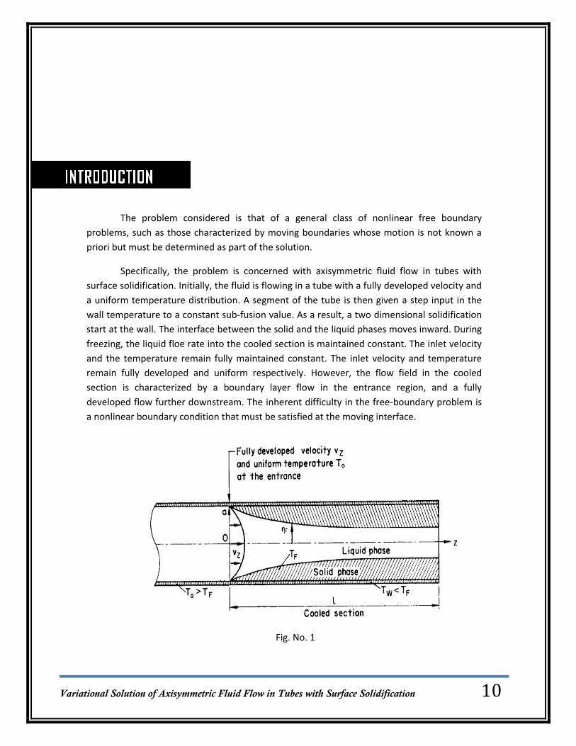
The problem considered is that of a general class of nonlinear free boundary

problems, such as those characterized by moving boundaries whose motion is not known a

priori but must be determined as part of the solution.

Specifically, the problem is concerned with axisymmetric fluid flow in tubes with

surface solidification. Initially, the fluid is flowing in a tube with a fully developed velocity and

a uniform temperature distribution. A segment of the tube is then given a step input in the

wall temperature to a constant sub-fusion value. As a result, a two dimensional solidification

start at the wall. The interface between the solid and the liquid phases moves inward. During

freezing, the liquid floe rate into the cooled section is maintained constant. The inlet velocity

and the temperature remain fully maintained constant. The inlet velocity and temperature

remain fully developed and uniform respectively. However, the flow field in the cooled

section is characterized by a boundary layer flow in the entrance region, and a fully

developed flow further downstream. The inherent difficulty in the free-boundary problem is

a nonlinear boundary condition that must be satisfied at the moving interface.

Fig. No. 1


11

A lot of research and scientific work has been done and established in the field in the

time gone by. The present state of work is very steady. To make note of some of the authors

and scientists who have put there remarkable hard in the field are too many.

Excellent literature reviews are given by Boley and Muehlbeuer and Suderland. Most

of these problems deal with a phase change without fluid flow or with external flow. Non-

flow problems usually are based on two coupled conduction equations to be satisfied in the

solid and liquid regions. The external flow problems ordinarily can be uncoupled, since the

field variables of the external phase are not significantly affected by the motion of the free

boundary.

Limited work has been done on problems involving internal flow with surface

solidification. In such systems, the dynamic and thermal response of liquid phase is directly

affected by the interface motion. Therefore, the field equations in both phases cannot be

uncoupled unless one of the phases is assumed to be at fusion temperature.

Grigorian has considered a special one-dimensional problem of melting due to

friction between two moving solid bodies. The problem was formulated in terms of the

equations of continuity, motion and energy in both phases. The problem has a self-similar

solution; therefore, an exact solution of the interface position was determined to within a

constant which was evaluated approximately for some limiting conditions.

Bowley and Coogan considered melting of two parallel quarter-infinite solids due to

an internal fluid flow between the solids. Bowley’s major restriction was that the solid region

be maintained at the melting temperature throughout. This allowed uncoupling of the

equations for the two regions. An integral method was used to transform the Cartesian field

equations of continuity, momentum and energy to a set of first-order nonlinear partial

differential equations which were then solved by quadrature.


12

Zerkle and Sunderland considered a steady-state case of fluid flow in tubes with

surface solidification. Experimental results were obtained and used to develop a semi-

empirical solution. A steady-state analytical solution was also determined. At steady state,

the interface is stationary. Zerkle made use of this and transformed the convection equation

to the classical Graetz form by assuming a parabolic velocity distribution. The coefficients of

the series solution were evaluated numerically.

Ozisik and Mulligan obtained a quasi-static solution to the freezing of liquids in

forced flow inside tubes. The problem was formulated in terms of a steady-state one-

dimensional conduction equation in the solid region, and a transient two-dimensional

convection equation in the liquid. The method of solution was based on the integral

transforms which could be used only with the assumption of slug velocity. According to

the authors, the applicability of their solution is restricted to the regions where the

rate of change of thickness of the frozen layers is small with respect to both time and

distance, along the tube (close to steady state and away from the entrance region).

Few free boundary problems have been solved exactly. Most solutions have been

obtained numerically or by approximate analytical methods. Of interest here are the

approximate variational methods. These methods, based on the minimum principle, have

been successfully applied in optics, dynamics, wave, mechanics, quantum mechanics and

Einstein’s law of gravitation. Helmholtz was probably the first to attempt to apply the

variational principles to thermodynamics; however, the minimum principles were not

directly applicable to the dissipative systems. Biot developed a method based on the

principle of minimum rate of entropy production and applied it to several one-

dimensional external flow problems. The method has also been applied by Lapadula

and Mueller to an external flow problem involving freezing over a flat plate. A more

general formulation of the variational principle, known as Lagrangian formalism, is usually

presented without reference to any specific system. The Lagrangian formalism may be

specialized to solve a diffusion or conduction equation. The variational solution presented in

this paper is based on the Lagrangian formalism. The, application of the method is

extended to solve the free-boundary problems involving internal flow.


13

The problem can be formulated in cylindrical coordinates in terms of a complete set

of field equations in the liquid and solid region; both of these regions being coupled by a set

of nonlinear boundary conditions to be satisfied at the moving liquid-solid interface. An order

of magnitude analysis of such a set shows that the axial conduction, axial viscous shear,

dissipation, body forces and radial pressure gradient may be neglected under the usual

conditions of the boundary layer flow.

Two variational solutions of the above problem are presented in this report. The first

variational solution, abbreviated as (V), is less accurate than the second, (VN), solution. The

less accurate solution (V) is presented because it is more general and also because its

examination permits the evaluation of several aspects of the physical problem.

Also author has used numerical solutions to solve the problem to compare the solution

obtained with that of the solutions obtained from variational formulations. Authors have

used this numerical solution tom plot various graphs to show different characteristics of the

problem. But these numerical solutions have not been included in the paper. Also, because of

the complexity of these solutions no attempt has been made to obtain them in this report.

Problem Statement s


14

Fig. No. 2

A 3D representation of the flow through the tube along with the surface solidification because

of presence of temperature gradient

Fig. No. 3

A 3D representation of the flow through the tube along with the surface solidification, by a

cross-section of the tube by cutting it along its axis, because of presence of temperature

gradient


15

Fig. No. 4

Configuration of the problem well explained by different notations, showing both – solid phase

as well liquid phase

The tube has been shown by brown colour and the portion inside the tube which has got

solidified because of variation in temperature present inside, has been shown by blue colour.

The rest of the pipe has water in liquid state.


16

For constant properties in each phase the boundary conditions imposed to the problem can

be given as:

* (

)

+

* (

)

+

Boundary Conditions Statement


17

Basic Principle

In steady flow, the mass flow per unit time passing through each section does not

change, even if the pipe diameter changes. This is the law of conservation of mass.

For the pipe shown here whose diameter decreases between sections 1 and 2, which

have cross-sectional areas A1, and A2 respectively, and at which the mean velocities are

and and the densities and respectively,

= or

= constant

If the fluid is incompressible, e.g. water, with being effectively constant, then

= constant

Continuity Equation

Fig. No. 5


18

Application to the Problem

Continuity equation in cylindrical coordinates can be presented as,

Considering density to be constant ), the above equation becomes

Since there is no vortex formation and the flow is irrotational, the situation can be reduced to

Converting and to dimensionless quantities, by using

We get the final equation as,

𝟏

𝑹 𝑹𝑽𝑹

𝝏

𝝏𝒁 𝑽𝒁 𝟎


19

Basic Principle

The dynamic behavior of fluid motion is governed by a set of equations, known as

equations of motion. These equations are obtained by using the Newton’s second law, which

may be written as

where is the net force acting in the x-direction upon a fluid element of mass producing

an acceleration of in the x-direction.

The forces which may be present in the fluid flow problems are: gravity force, pressure force,

force due to viscosity, force due to turbulence, and the force due to compressibility of fluid.

When volume changes are small, the force due to compressibility is negligible , and the

general equation of motion in the x-direction using previous equation may be written as

Similar expressions for y and z- directions may also be written. When we substitute the

expressions for various quantities in this equation, the resulting equations are known as

Reynolds equations.

For flow at low Reynolds number, the force due to turbulence is of no significance and,

therefore, pressure force and the viscous force is

together with similar expressions for y and z-directions are known as the Navier-Stokes

equations.

Equation of Motion


20

Thus Navier-Stokes equation in Cartesian form can be written as

(

)

{ (

)}

{ (

)}

Similarly expressions for y and z-directions can be obtained.


21


Equation of motion along z-axis in cylindrical coordinates is given as

(

)

*

(

)

+

Since the given flow condition is irrotational and the body forces have been assumed to be

zero, thus

(

)

*

(

)

+

(

)

*

+

(

)

Also, axial viscous shear is zero, and thus the last term can be put to zero resulting into

(

)

*

+

After transforming and into dimensionless quantities and making substitution using,

We get the final result as

𝟏

𝜶𝑷𝒆

𝝏𝑽𝒁𝝏𝝉

(𝑽𝑹𝝏𝑽𝒁𝝏𝑹

𝑽𝒁𝝏𝑽𝒁𝝏𝒁

) 𝝏𝑷

𝝏𝒁

𝟏

𝑹𝒆

𝟏

𝑹

𝝏

𝝏𝑹(𝑹

𝝏𝑽𝒁𝝏𝑹

)


22

Basic Principle

For solid phase, the energy equation when combined with Fourier’s Law of heat

conduction, becomes

If the thermal conductivity can be assumed to be independent of the temperature and

position, then above equation becomes

in which is the thermal diffusivity of the solid.

Energy Equation in Solid Phase


23


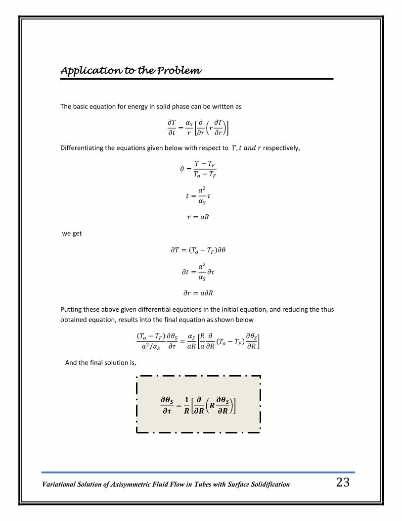
The basic equation for energy in solid phase can be written as

[

(

)]

Differentiating the equations given below with respect to respectively,

we get

Putting these above given differential equations in the initial equation, and reducing the thus

obtained equation, results into the final equation as shown below

[

]

And the final solution is,

𝝏𝜽𝑺𝝏𝝉

𝟏

𝑹[𝝏

𝝏𝑹(𝑹

𝝏𝜽𝑺𝝏𝑹

)]


24

Basic Principle

While considering the liquid phase, the velocity effects of the liquid will come into

the picture. Thus, making slight amendments will give us the energy equation in liquid phase.

The desired equation in Cartesian form can be given as,

(

) (

)

Addition of axial velocity and radial velocity will serve our purpose in order to obtain the

energy equation in cylindrical coordinates.

Energy Equation in Liquid Phase


25


Energy equation in liquid phase is as shown below,

(

)

(

)

Dividing the above equation by throughout, we obtain

(

)

(

)

Changing to dimensionless quantities, we obtain

(

)

(

)

The resulting equation after simplification is,

𝟏

𝜶𝑷𝒆

𝝏𝑻

𝝏𝝉 𝑽𝑹

𝝏𝑻

𝝏𝑹 𝑽𝒁

𝝏𝑻

𝝏𝒁

𝟏

𝑷𝒆

𝟏

𝑹

𝝏

𝝏𝑹(𝑹

𝝏𝑻

𝝏𝑹)


26

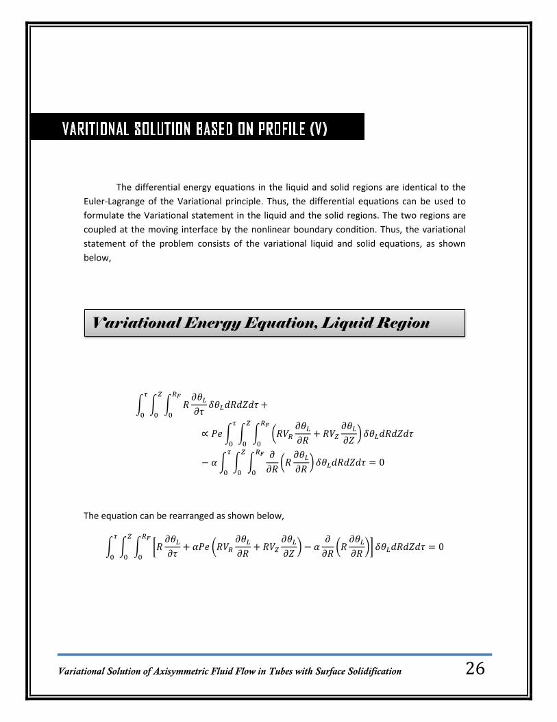
The differential energy equations in the liquid and solid regions are identical to the

Euler-Lagrange of the Variational principle. Thus, the differential equations can be used to

formulate the Variational statement in the liquid and the solid regions. The two regions are

coupled at the moving interface by the nonlinear boundary condition. Thus, the variational

statement of the problem consists of the variational liquid and solid equations, as shown

below,

∫ ∫ ∫

∫ ∫ ∫ (

)

∫ ∫ ∫

(

)

The equation can be rearranged as shown below,

∫ ∫ ∫ [

(

)

(

)]

Variational Energy Equation, Liquid Region


27

If varies invariably, then the term in square brackets can be put to zero i.e.

[

(

)

(

)]

The profile which has been used for solving this physical problem is,

using which different parts of the equation can be simplified as,

{

}

(

)

{

}

(

)

It is to be noted that here and .

Adding above and equating to zero and further reduction gives,

𝑓 𝑥 𝑦 𝑧 𝛿𝑉𝑑𝑥𝑑𝑦𝑑𝑧

𝑓 𝑥 𝑦 𝑧

For a given integration as given below,

If the functional 𝛿𝑉 varies without any restriction for all values of x, y, z ; then only

option we are left are with is that


28

Now subjecting the above equation to the following initial conditions,

(at )

The equation becomes,

Finally we obtain the resulting equation as,

Now comparing the result with that obtained by the authors of the paper, we see that

assigning and

will serve the purpose.

Hence, the final result will be,

(

)

𝝏𝑪

𝝏𝝉

𝟑𝑪

𝑹 𝑭

𝝏𝑹𝑭𝝏𝝉

𝟔𝜶𝑪

𝑹𝑭𝟐

𝜶𝑷𝒆(𝟗

𝟐

𝑪

𝑹𝑭𝟑

𝝏𝑹𝑭𝝏𝒁

𝟑

𝟐

𝟏

𝑹𝑭𝟐

𝝏𝑪

𝝏𝒁)


29

But the actual result as obtained by the authors, is

𝝏𝑪

𝝏𝝉

𝟑𝑪

𝑹 𝑭


𝟔𝜶𝑪

𝑹𝑭𝟐

𝜶𝑷𝒆(𝟑𝑪

𝑹𝑭𝟑

𝝏𝑹𝑭𝝏𝒁

𝟑

𝟐

𝟏

𝑹𝑭𝟐

𝝏𝑪

𝝏𝒁)


30

∫ ∫ ∫

∫ ∫ ∫

(

)

The equation can be rearranged as show below,

∫ ∫ ∫ [

(

)]

If varies invariably, then the term in square brackets can be put to zero i.e.

[

(

)]

The profile which has been used for solving this physical problem,

𝑓 𝑥 𝑦 𝑧 𝛿𝑉𝑑𝑥𝑑𝑦𝑑𝑧

𝑓 𝑥 𝑦 𝑧

For a given integration as given below,

If the functional 𝛿𝑉 varies without any restriction for all values of x, y, z; then only

option we are left are with is that

Variational Energy Equation, Solid Region


31

using which different parts of the above expression can be simplified as,

*

+

(

)

Thus,

*

+

Now rearranging the above equation we obtain,

But the expression obtained by the authors can be shown as below,

𝝏𝑩

𝝏𝝉 𝜽𝒘


[𝟏

𝟏 𝑹𝑭 𝟐 𝑹 𝑹𝑭 ] 𝑩 (

𝟏

𝟏 𝑹𝑭)𝝏𝑹𝑭𝝏𝝉

[𝜽𝒘

𝑹 𝑹 𝟏 𝟏 𝑹𝑭 𝑹 𝑹𝑭 ] 𝑩 [

𝟒𝑹 𝑹𝑭 𝟏

𝑹 𝑹 𝟏 𝑹 𝑹𝑭 ]

𝝏𝑩

𝝏𝝉 𝜽𝒘


* 𝟐 𝟑𝑹𝑭

𝟏 𝑹𝑭 𝟑 𝟏 𝑹𝑭 + 𝑩


* 𝟐 𝟑𝑹𝑭

𝟏 𝑹𝑭 𝟏 𝑹𝑭 +

[𝟏𝟎𝜽𝒘

𝟏 𝑹𝑭 𝟏 𝑹𝑭 𝟑] [

𝟏𝟎𝑩

𝟏 𝑹𝑭 𝟐]


32

Basic Principle

If the fluid and flow characteristics such as density, velocity, pressure, acceleration

etc., at a point do not change with time, the flow is said to be steady, thus for steady flow

(

)

(

)

(

)

and so on.


33


For steady state solution, the characteristic equations for fluid flow conditions in

concerned problem will have all the time derivatives equal to zero, i.e.

Considering the first solution obtained from the Variational energy equation in liquid region,

(

)

and putting all time derivatives equal to zero, in order to obtain a steady state solution, we

get

(

)

(

)

(

)

Now by using separation of variable technique,

(

)

𝜕

𝜕𝜏

First Solution


34

On integrating we obtain,

√

where, represents constant of integration.

Simplification of the result,

And its comparison with the actual one shows that the constant of integration has a

value

.

𝑪∞ 𝒁 𝟏

𝝃𝑹𝑭∞

𝟐𝒆𝒙𝒑 (

𝟒𝒁

𝑷𝒆)

𝑪∞ 𝒁 𝟏 𝟓

𝑹𝑭∞

𝟐𝒆𝒙𝒑 (

𝟒𝒁

𝑷𝒆)


35

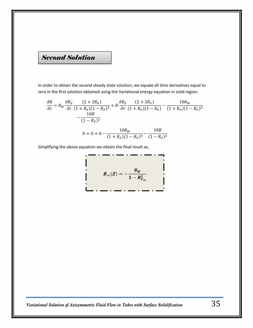
In order to obtain the second steady state solution, we equate all time derivatives equal to

zero in the first solution obtained using the Variational energy equation in solid region.

Simplifying the above equation we obtain the final result as,

𝑩∞ 𝒁

𝜽𝑾

𝟏 𝑹𝑭∞

𝟐

Second Solution


36

Now moving to the 2nd solution obtained from the Variational energy equation in the solid

region, we again employ the same strategy in order to obtain the steady state solution.

[

] * (

)

+

[

] * (

)

+

Seeing above,

[

]

since [ (

) ] will always be positive and greater than zero.

Now substituting the expressions for B and C, from the steady state solutions obtained above,

the equation transforms into

(

)

This transforms into a quadratic equation,

where

(

)

(

)

Third Solution


37

Solving this quadratic equation we obtain the roots of the equation as,

(

) , [

(

)]

-

Neglecting the negative sign in the above, final solution will be

𝑹𝑭 𝜽𝑾𝟑𝑲

𝒆𝒙𝒑 (𝟒𝒁

𝑷𝒆) ,𝟏 [

𝜽𝑾𝟑𝑲

𝒆𝒙𝒑 (𝟒𝒁

𝑷𝒆)]𝟐

-

𝟏 𝟐


38

In order to obtain the very first short time solution of variational solutions based on

profiles (V), we consider the equation,

[

] * (

)

+

The first solution is based on zero convection and linear .

Thus,

, since has been considered to be linear

, zero convection

, when there is no convection taking place, the interface position will not

change with respect to axial distance

Hence, the equation reduces to,

(

)


39

Now integrating the above equation, we obtain

√(

)

So, the resulting solution obtained is

This solution is applicable for relatively short time, when the solid phase thickness

∞ .

𝑹𝑭 𝟏 √( 𝟐𝜽𝑾𝝀

𝝉)


40

The Variational solution obtained here is based on Nusselt number. The profiles for

and is same as that used previously. However, the profile for is replaced by a mean

liquid temperature and a Nusselt number .Thus, the Variational statement of

the problem remains same except that Variational energy equation in the liquid region is

replaced by an integral energy equation in terms of and .

∫ ∫

∫

∫ ∫ (

)

Bringing all the terms on the left hand side,

∫ ∫

∫

∫ ∫ (

)

Or,

∫

∫ (

)

Integral Energy Equation, Liquid Region


41

Substituting and

*

+ in the above expression, we obtain

∫

∫ (

*

+

)

Integration of the above equation with respect to R, will give us

*

+

Rearrangement of the above terms, will result into

The same solution as obtained by the authors is,

𝝏𝜽𝑴𝝏𝝉

𝟐𝜶𝑵𝜽𝑴

𝑹𝑭𝟐

𝟐 𝑷𝒆

𝑹𝑭𝟐

𝝏𝜽𝑴𝝏𝒁

𝝏𝜽𝑴𝝏𝝉

𝟐𝜶𝑵𝜽𝑴

𝑹𝑭𝟐

𝟒 𝑷𝒆

𝑹𝑭𝟐

𝝏𝜽𝑴𝝏𝒁

[𝟏

𝟐

𝟏

𝟑𝑹𝑭]


42

Basic Principle

If the fluid and flow characteristics such as density, velocity, pressure, acceleration

etc., at a point do not change with time, the flow is said to be steady, thus for steady flow

(

)

(

)

(

)

and so on.


43


For steady state solution, the characteristic equations for fluid flow conditions in

concerned problem will have all the time derivatives equal to zero, i.e.

First steady state solution can be obtained by equating time derivatives in the equation

equal to zero. Thus, we have

The expression for Nusselt number in terms of dimensionless axial coordinate, Peclet number

and other constants can be given as

[

]

𝜕

𝜕𝜏

First Solution


44

Hence substituting the expression of in the above equation, we get

[

]

[

]

[

]

* (

)

+

* (

)

+

*

(

)

+

Thus, rearranging the above, final result will be as shown below

𝜽𝑴∞ 𝒁 *𝟏

𝟏

𝒄(𝒁

𝑷𝒆)𝟐 𝟑

+

𝟑𝒂𝒃

𝒆𝒙𝒑 [ 𝟐𝒂 (𝒁

𝑷𝒆)]


45

Similarly the second steady state solution can be obtained from the equation

[

] * (

)

+

[

] * (

)

+

Since,

* (

)

+

thus,

[

]

Substituting the expression for B in the above equation gives us

It is a quadratic equation, whose roots will lend us the required results.

Hence, the solution is

𝑹 𝜽𝑾

𝑲𝑵𝜽𝑴 *𝟏 (

𝜽𝑾𝑲𝑵𝜽𝑴

)𝟐

+

𝟏 𝟐

Second Solution


46

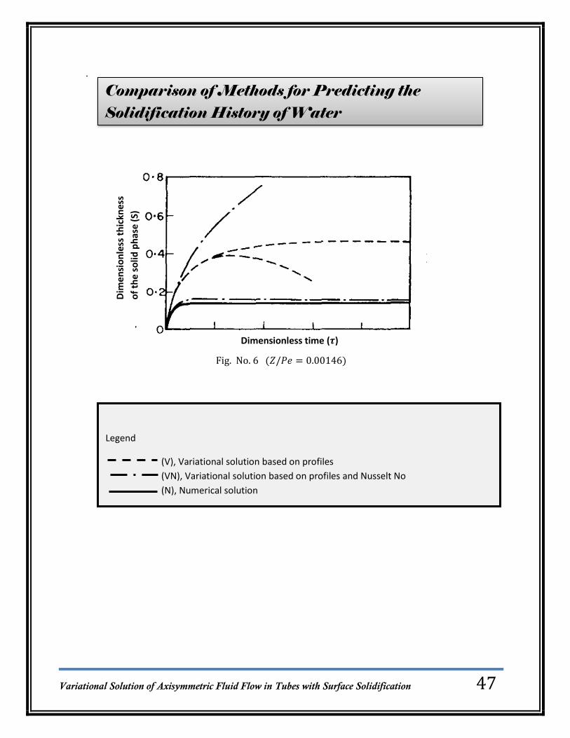
In order to compare and analyze the problem graphically, the authors have used three

different solutions to obtain the results and have them plotted for short time, asymptotic and

steady state composite parts.

For the research paper originally three solutions were obtained, which are as follows:

Variational solution based on profiles

Variational solution based on profiles and Nusselt no.

Numerical solution

But only two solutions have been given in the paper from the above. No data or expressions

used regarding Numerical solution have been included. Also, there is no expression explaining

the relationship of dimensionless thickness of solid phase with dimensionless

time .

The validity of variational solution (V) is limited only in the entrance region. The (VN) solution

is generally more accurate and therefore is preferred to the variational solution (V).

In spite of these limitations, it has been tried to explain the graphs, when and wherever

possible.


47

.

Fig. No. 6

Legend

(V), Variational solution based on profiles

(VN), Variational solution based on profiles and Nusselt No

(N), Numerical solution

Comparison of Methods for Predicting the Solidification History of Water

𝜏Type equatio here

Dimensionless time (𝝉)

Dim

en

sio

nle

ss t

hic

knes

s

of

the

solid

ph

ase

(S)


48

Fig. No. 7

Fig. No. 8



Dim

en

sio

nle

ss t

hic

knes

s

of

the

solid

ph

ase

(S)

Dim

en

sio

nle

ss t

hic

kne

ss

of

the

solid

ph

ase

(S)


49

Fig. No. 9

Fig. No. 10

Comparison of Methods for Predicting the Axial Distribution of Ice Layer

Normalized distance from entrance region (Z/Pe)


Dim

en

sio

nle

ss t

hic

knes

s

of

the

solid

ph

ase

(S)

Dim

en

sio

nle

ss t

hic

kne

ss

of

the

solid

ph

ase

(S)


50

Dim

en

sio

nle

ss t

hic

knes

s

of

the

solid

ph

ase

(S)


Fig. No. 11

Legend



(N), Numerical solution


51

Comparison of Limiting Transient Solutions with Available Non-flow Data


Dim

en

sio

nle

ss t

hic

kne

ss o

f th

e so

lid p

has

e (

S)

Fig. No. 12


52

Legend

Numerical solution, 𝑅𝑒𝐷 𝜌 𝑇 𝑇𝐹 ℉

Short time solution based on zero convection and linear 𝜃𝑆 profile

Short time solution based on zero convection and non-linear 𝜃𝑆 profile

Poots integral solution-Karman method

Poots integral solution-Tani method

Allen and Severn numerical solution

(Based on initial 𝜃𝐿 𝜆𝑊 𝐿

𝐶𝑆 𝑇𝐹 𝑇𝑊 𝜌

𝜌𝐿 𝜌𝑆

𝜌𝐿 )


53

Comparison of Limiting Solutions with Available Steady-State Data


No

rmal

ize

d in

terf

ace

po

siti

on

𝑹𝑭

𝑲 𝜽

𝑾

Fig. No. 13


54

Legend



(N), Numerical solution 𝑅𝑒𝐷

Zerkle’s analytical steady state solution

Zerkle’s semi-empirical steady state data, 𝑅𝑒𝐷

Ozisik-Mulligan steady state solution


55

Comparison of Variational Solutions Based on Different Profiles


Dim

en

sio

nle

ss s

tead

y-st

ate

th

ickn

ess

of

the

solid

ph

ase

(S)

Fig. No. 14


56

Legend



(V), Numerical solution 𝑅𝑒𝐷

(V), based on 2-parameters 𝜃𝐿

(V), based on slug 𝑉𝑍

(V), based on linear 𝜃𝑆


57

The effect of natural convection cannot be fully evaluated here since it is not

considered in any solution presented here.

The study can be used to make modifications in the current scenario of cold storage.

It will beneficial to those countries where there is serious problem of solidification of water

pipe lines and water in engine radiators.


58

A cylindrical coordinate system is a three-dimensional coordinate system that

specifies point positions by the distance from a chosen reference axis, the direction from the

axis relative to a chosen reference direction, and the distance from a chosen reference plane

perpendicular to the axis. The latter distance is given as a positive or negative number

depending on which side of the reference plane faces the point.

The origin of the system is the point where all three coordinates can be given as zero. This is

the intersection between the reference plane and the axis.

The axis is variously called the cylindrical or longitudinal axis, to differentiate it from the polar

axis, which is the ray that lies in the reference plane, starting at the origin and pointing in the

reference direction.

The distance from the axis may be called the radial distance or radius, while the angular

coordinate is sometimes referred to as the angular position or as the azimuth. The radius and

the azimuth are together called the polar coordinates, as they correspond to a two-

dimensional polar coordinate system in the plane through the point, parallel to the reference

plane. The third coordinate may be called the height or altitude (if the reference plane is

considered horizontal), longitudinal position, or axial position.

Cylindrical coordinates are useful in connection with objects and phenomena that have some

rotational symmetry about the longitudinal axis, such as water flow in a straight pipe with

round cross-section, heat distribution in a metal cylinder, and so on.

Cylindrical Coordinates

http://en.wikipedia.org/wiki/Coordinate_system

http://en.wikipedia.org/wiki/Line_(mathematics)#Ray

http://en.wikipedia.org/wiki/Polar_coordinates

http://en.wikipedia.org/wiki/Symmetry

http://en.wikipedia.org/wiki/Cylinder_(geometry)


59

Definition

The three coordinates (ρ, φ, z) of a point P are defined as:

The radial distance ρ is the Euclidean distance from the z axis to the point P.

The azimuth φ is the angle between the reference direction on the chosen plane and the line from the origin to the projection of P on the plane.

The height z is the signed distance from the chosen plane to the point P.

Coordinate system conversions into Cartesian coordinates

For the conversion between cylindrical

and Cartesian coordinate systems, it is

convenient to assume that the reference

plane of the former is the Cartesian x–y

plane (with equation z = 0), and the

cylindrical axis is the Cartesian z axis.

Then the z coordinate is the same in both

systems, and the correspondence

between cylindrical (ρ, φ) and Cartesian

(x, y) are the same as for polar

coordinates, namely

os

si

in one direction, and

√

{

si (

)

si (

)

Fig. No. 15

http://en.wikipedia.org/wiki/Rho_%28letter%29

http://en.wikipedia.org/wiki/Phi

http://en.wikipedia.org/wiki/Euclidean_distance


60

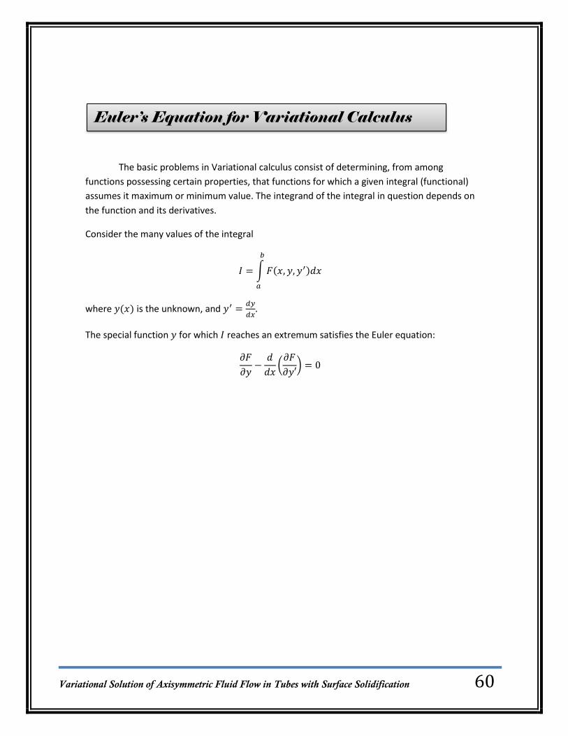
The basic problems in Variational calculus consist of determining, from among

functions possessing certain properties, that functions for which a given integral (functional)

assumes it maximum or minimum value. The integrand of the integral in question depends on

the function and its derivatives.

Consider the many values of the integral

∫

where is the unknown, and

The special function for which reaches an extremum satisfies the Euler equation:

(

)

Euler’s Equation for Variational Calculus


61

1. J. A. Bilenas and L. M. Jiji, “Variational Solution Of Axisymmetric Fluid Flow In Tubes

With Surface Modification”, Ph.D. thesis, City University of New York, New York, 1968.

2. Heat Transfer (2nd edition), by Cengel.

3. Transport Phenomena (2nd edition), by R. B. Bird, W. E. Stewart and E. N. Ligthfoot.

4. Fluid Mechanics, by Dr. A. K. Jain.

5. Higher Engineering Mathematics, by Dr. B. S. Grewal.

6. Wikipedia (free encyclopedia), http://en.wikipedia.org.

7. Wolfram Mathworld, http://mathworld.wolfram.com.

variational solution of axisymmetric fluid flow in tubes with surface solidification

Engineering

variational energy equation

variational calculus

problem23 energy equation

eulers equation

continuity equation

equation of motion

liquid phase24 basic

solid region30 basic