a simulation of mpsk communications system performance in

Calhoun: The NPS Institutional Archive

Theses and Dissertations Thesis Collection

1998-12

A simulation of MPSK communications system

performance in the presence of wideband noise and

co-channel interference

Erdogan, Veysel

Monterey, California: Naval Postgraduate School

http://hdl.handle.net/10945/39319

NAVAL POSTGRADUATE SCHOOL Monterey, California

THESIS

A SIMULATION OF MPSK COMMUNICATIONS SYSTEM PERFORMANCE IN THE PRESENCE OF WIDEBAND

NOISE AND CO-CHANNEL INTERFERENCE

Thesis Advisor: Thesis Co-Advisor:

by

Veysel Erdogan

December 1998

Jovan Lebaric Clark Robertson

Approved for public release; distribution is unlimited.

c:> c:> ......,..

REPORT DOCUMENTATION PAGE Form Approved OMB No. 0704-

0188

Public reporting burden for this collection of information is estimated to average 1 hour per response, including the time for reviewing instruction, searching existing data sources, gathering and maintaining the data needed, and completing and reviewing the collection of information. Send comments regarding this burden estimate or any other aspect of this collection of information, including suggestions for reducing this burden, to Washington headquarters Services, Directorate for Information Operations and Reports, 1215 Jefferson Davis Highway, Suite 1204, Arlington, VA 22202-4302, and to the Office of Management and Budget, Paperwork Reduction Project (0704-0188) Washington DC 20503.

1. AGENCY USE ONLY (Leave blank) 2. REPORT DATE 3. REPORT TYPE AND DATES

December 1998 COVERED Master's Thesis

4. TITLE AND SUBTITLE 5. FUNDING A SIMULATION OF MPSK COMMUNICATIONS SYSTEM PERFORMANCE IN THE NUMBERS

PRESENCE OF WIDEBAND NOISE AND CO-CHANNEL INTERFERENCE

6. AUTHOR(S)

Erdogan, Veysel

7. PERFORMING ORGANIZATION NAME(S) AND ADDRESS(ES) 8. PERFORMING ORGANIZATION

Naval Postgraduate School REPORT NUMBER Monterey, CA 93943-5000

9. SPONSORING I MONITORING AGENCY NAME(S) AND ADDRESS(ES) 10. SPONSORING I MONITORING AGENCY REPORT NUMBER

11. SUPPLEMENTARY NOTES

The views expressed in this thesis are those of the author and do not reflect the official policy or position of the Department of Defense or the U.S. Government.

12a. DISTRIBUTION I AVAILABILITY STATEMENT 12b.

Approved for public release; distribution is unlimited. DISTRIBUTION CODE

13. ABSTRACT (maximum 200 words) The purpose of this research is to model digital communications systems in the time domain using

MATLAB Simulink and the Communications Toolbox and to determine and verify the system performance in the presence of additive noise and interference.While the theoretical results are available for the assesment of the influence of wideband gaussian noise on the performance of a digital communications system,determining the performance of a system in the presence of noise and interference requires a computer simulation.The time domain modeling allows the visualisation of communication signals at various stages of transmitters and receivers and "Monte C.arlo" type simulations to establish the bit error rates under realistic conditions (noise, interference) and for different values of transmitter/receiver parameters, different channel parameters and different types of interfering signals. It should be noted that the simulation does not account for system non-linearities. 14. SUBJECTTERMS Simulink,Matlab, Noise and Interference, Probability of Bit Error

17. SECURITY CLASSIFICATION OF 18. SECURITY CLASSIFICATION OF

REPORT THIS PAGE

Unclassified Unclassified

NSN 7540-01-280-5500

15. NUMBER OF PAGES

118

16. PRICE CODE

19. SECURITY CLASSIFI-20.

CATION OF ABSTRACT LIMITATION OF

Unclassified ABSTRACT

UL

Standard Form 298 (Rev. 2-89) Prescribed by ANSI Std.

Approved for public release; distribution is unlimited

A SIMULATION OF MPSK COMMUNICATIONS SYSTEM PERFORMANCE IN THE PRESENCE OF WIDEBAND NOISE AND CO-CHANNEL INTERFERENCE

Veysel Erdogan First Lieutenant, Turkish Army

B.S., Turkish Military Academy, 1991

Submitted in partial fulfillment of the requirements for the degree of

MASTER OF SCIENCE IN ELECTRICAL ENGINEERING

Approved by:

from the

NAVAL POSTGRADUATE SCHOOL December 1998

/Clark Robertson, Thesis Co-Advisor

Jeffrey . Knorr, Chairman Department of Electrical Engineering

iii

ABSTRACT

1:he purpose of this thesis is to model digital communications systems in the time

domain using MATLAB Simulink and the Communications Toolbox as well as to

determine and verify system performance in the presence of additive noise and co

channel interference. While the theoretical results are available for the effect of wideband

gaussian noise on the performance of digital communications systems, determining the

performance of a system in the presence of noise and co-channel interference is best done

by computer simulation. Time domain modeling allows the visualization of the

communication signal at various stages, and "Monte Carlo" type simulations establish the

bit error rates under realistic conditions of noise and co-channel interference as well as

for different transmitter/receiver parameters, different channel parameters, and different

types of interfering signals. It should be noted that the simulation does not account for

system non-linearities.

v

TABLE OF CONTENTS

l IN'fR.ODUCTION ................................................................................ 1

Il. SIMULINK AND THE COMMUNICATIONS TOOLBOX ........................................ 3

Ill PHASE-SIIIF'T-KEYING ............................................................................................. 5

A BINAR.Y PHASE-SIIIF'T-KEYING ......................................................................... 5

B. SIGNAL CONSTELLATION FOR BPSK .............................................................. ·. 6

C. PROBABILITY OF BIT ERROR FOR BPSK ......................................................... 7

D. QUADRATURE PHASE-SIIIF'T-KEYING ........................................................... 10

E. SIGNAL CONSTELLATION FOR QPSK ............................................................. 11

F. PROBABILITY OF BIT ERROR FOR QPSK ...................................................... 12

G. SIMULINK MODEL OF MPSK DIGITAL COMMUNICATION SYSTEM ....... 12

N. BIT ERROR PROBABILITY CONVERGENCE ................................................... 17

V. SIMULATION VERIFICATION FOR BPSK AND QPSK WITH AWGN ........... 31

A BPSK BIT ERROR PROBABILITY ESTIMATES .............................................. 33

1.BPSK Results for the Simulink Model ................................................................ 33

2.BPSK Results Obtained by Using Matlab Program MPSKl.M .............................. 35

B. QPSK BIT ERROR PROBABILITY ESTIMATES ............................................... 38

l.QPSK Results for the Simulink Model ............................................................... 38

2.QPSK Results Obtained by Using Matlab Program MPSKl.M .............................. 39

vii

VI. SIMULATION VERIFICATION FOR BPSK AND QPSK WITH ADDITIVE

WHITE GAUSSIAN NOISE AND CO-CHANNEL INTERFERENCE ......................... 41

A. BPSK BIT ERROR PROBABILITY ESTTh1ATES ............................................. .41

l.BPSK Results for the Simulink Model ................................................................ 43

2.BPSK Results Obtained by Using Matlab Program :MPSKl .M .............................. 46

B. QPSK BIT ERROR PROBABILITY ESTTh1ATES ............................................... 49

1.QPSK Results for the Simulink Model ..................... ~ ......................................... 49

2.QPSK Results Obtained by Using Matlab Program:MPSKl.M .............................. 52

VII. CONCLUSIONS AND RECOMMENDATIONS ......................... : .......................... 57

A. CONCLUSIONS ............ ··················································································.········· 57

B. RECOMMENDATIONS ............................................... · ............................................ 58

APPENDIX A. BATCH_RUN.M MATLAB PROGRAM FOR CONVERGENCE TEST

OF SIMULATION USING BPSK .................................................................................... 59

APPENDIX B. BER_PLOT.M MATLAB PROGRAM FOR PLOTTING THE

FIGURES OF THE SIMULATION FOR EACH VARIANCES ..................................... 61

APPENDIX C. PLOT_STh1_NOISE2 MATCHAD PROGRAM FOR RESULTS OF

NOISE ONLY CASE BPSK USING SWULINK MODEL ............................................ 63

viii

APPENDIX D. PLOT_MAT_NOISE2 MATCHAD PROGRAM FOR RESULTS OF

NOISE ONLY CASE BPSK USING MATLAB PROGRAM ......................................... 65

APPENDIX E. PLOT_SIM_NOISE4 MATCHAD PROGRAM FOR RESULTS OF

NOISE ONLY CASE QPSK USING SIMULINK MODEL ............................................ 67

APPENDIX F. PLOT_MAT_NOISE4 MATCHAD PROGRAM FOR RESULTS OF

NOISE ONLY CASE QPSK USING MATLAB PROGRAM ......................................... 71

APPENDIX G. PLOT_SIM_NOISE&INT2 MATCHAD PROGRAM FOR RESULTS

OF NOISE AND INTERFERENCE CASE BPSK USING SIMULINK MODEL .......... 75

APPENDIX H. PLOT_MAT_NOISE&INT2 MATCHAD PROGRAM FOR RESULTS

OF NOISE AND INTERFERENCE CASE BPSK USING MATLAB PROGRAM ....... 79

APPENDIX I. PLOT_SIM_NOISE&INT4 MATCHAD PROGRAM FOR RESULTS

OF NOISE AND INTERFERENCE CASE QPSK USING SIMULINK MODEL .......... 83

APPENDIX J. PLOT_MAT_NOISE&INT4 MATCHAD PROGRAM FOR RESULTS

OF NOISE AND INTERFERENCE CASE QPSK USING MATLAB PROGRAM ....... 87

APPENDIX K. PREP ARE.M MATLAB PROGRAM TO ENTER THE SYSTEM

PARAMETERS TO BE USED BY THE SIMULINK MODEL ...................................... 91

APPENDIX L. MPSK.M MATLAB PROGRAM TO START SIMULATION ........... ~. 93

ix

APPENDIX M. MPSKl.M MATLAB PROGRAM FOR USING MATLAB PROGRAM

OPTION VICE SIMULINK MODEL ............................................................................... 95

LIST OF REFERENCES ................................................................................................ 101

BIBLIOGRAPHY ........................................................................................................... 103

INITIAL DISTRIBUTION LIST ..................................................................................... 105

x

ACKNOWLEDGMENT

I would like to thank all that contributed to and helped me prepare this thesis: Dr.

Jovan Lebaric for his support and advice and Prof. Clark Robertson whose knowledge in

Communications helped a lot in my studies.

Second I would like to thank my family in Turkey, for their constant support and

encouragement to accomplish this hard work.

Lastly I want to thank my country and Turkish Armed Forces for sending me to

NPS to have this education and opportunity. NPS not only gave me a good technical

knowledge but also awarded me a different way of looking at life.

xi

I. INTRODUCTION

A military site or a platform typically has a large number of communication

systems operating simultaneously in both transmit and receive modes. The interference

of one system with another depends on available frequency allocations, the physical

separation of transmit and receive antennas, non-linearity of transmitter output stages, and

so on. The objective of this study is to obtain a computer-based prediction of noise and

co-channel interference effects on the probability of bit error for M-ary Phase Shift

Keying (MPSK) digital communication systems. To accomplish this, a model was

developed using SIM:ULINK and the Communications Toolbox. The performance of the

model has been verified by comparing the simulation results and the theoretical results for

the bit error probability in the presence of additive white Gaussian noise (A WGN). The

model has been subsequently modified to include co-channel interference, and the bit

error probability of MPSK with A WGN and co-channel interference was obtained via

simulation.

1

II. SIMULINK AND THE COMMUNICATIONS TOOLBOX

SIMULINK is a program for modeling linear and non-linear dynamic systems in

the time-domain. Models in SIMULINK are represented in block-diagram form and can

be assembled from block libraries and sub-libraries. Furt_hermore, STh1ULINK allows the

display of results and changes of certain model parameters without interrupting the

simulation. Since SIMULINK is built upon the MATLAB numeric computation system,

it offers direct access to the MATLAB workspace and MATLAB' s mathematical and

engineering functions. SIMULINK' s main features are:

• modeling and analysis of dynamic systems, including linear, nonlinear,

continuous, discrete, and hybrid

• flexible "open system" environment that allows addition of new blocks to

Simulink

• seamless interface with MATLAB's built-in math functions, 2-D and 3-D

graphics, and add-on toolboxes for specialized applications

• choice of methods of running a simulation (menu-driven on-screen or batch

mode)

• an optimized computer platform implementation that ensures fast and accurate

results

• unlimited model size.

A typical STh1ULINK session starts by either defining a new model or recalling a

previously defined model and then proceeds to a simulation of the performance of that

3

model. fu practice these two steps are often performed iteratively as the model designer

creates and modifies a model to achieve the desired behavior [Ref. l].

The Communications Toolbox is a collection of MATLAB functions and

STh1ULINK blocks for model development and simulation in the communications area.

The functions/blocks are organized in the following sub-categories: Data Source, Source

Coding and Decoding, Error-Control Coding, Modulation and Demodulation,

Transmission and Reception filters, Transmitting Channel, Multiple Access, and

Synchronization and Utilities [Ref.1].

4

ID. PHASE SHIFT KEYING

Modulation of a sinusoidal carrier allows the conveyance of information in binary

form. The baseband information bit stream modulates the carrier by means of discrete

changes in the carrier amplitude (amplitude-shift keying or ASK) carrier frequency

(frequency-shift keying or FSK) or carrier phase (phase-shift keying or PSK) or some

combination of the above. Each different state of the carrier, known as a symbol,

corresponds to one or more bits of baseband information [Ref 2.].

A. BINARY PHASE-SHIFT KEYING

In binary phase-shift keying (BPSK), the phase of a constant amplitude carrier

signal is switched between two values according to the two possible "messages". m1 and

mz corresponding to binary 1 and 0, respectively. Normally, the two phases are separated

by 180degrees. If the sinusoidal carrier has amplitude Ac, then the average energy per bit

Eb = ~ A;rb, and the transmitted BPSK signal can be represented as:

0 $ t $ Tb ( binary 1) (1)

(binary 0) (2)

( binaryO) (3)

5

where Eb is the average energy per bit, Tb is the bit duration, and a rectangular pulse

shape p(t)=7Z[(t-T,,/2)/7;,)] is assumed. For this signal set, the single waveform

¢i (t) = {I cos(27ifct) vr: (4)

can be defined. Using this signal, the BPSK signal set can be represented as

S BPSK = {.[i;<Pi (f),-.fi:</J1 (f)} (5)

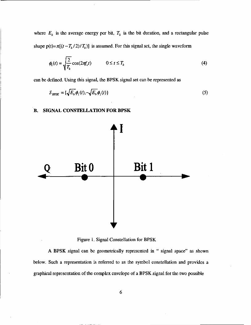
B. SIGNAL CONSTELLATION FOR BPSK

l

BitO Bit 1

Figure 1. Signal Constellation for BPSK

A BPSK signal can be geometrically represented in " signal space" as shown

below. Such a representation is referred to as the symbol constellation and provides a

graphical representation of the complex envelope of a BPSK signal for the two possible

6

symbols. The x-axis of the constellation diagram represents the "in-phase" component of

the complex envelope, and the y-axis represents the "quadrature" component of the

complex envelope. The distance between the signals on a constellation diagram indicates

how different the modulation waveforms are and determines how well a receiver can

differentiate between all possible symbols when random noise is present. The larger the

signal distance, the better the chance of correct symbol detection.

C. PROBABILITY OF BIT ERROR FOR BPSK

. An important measure of performance used for digital modulation is the

probability of symbol error, PE . It is often convenient to specify system performance by

the probability of bit error PB, even when decisions are made on the basis of symbols

rather than bits. The relationship between PB and PE for orthogonal signaling is:

(6)

For the BPSK modulation (M=2), the symbol error probability is equal to the bit

error probability. When the signals are assumed equally likely and signal s;(t)(i=l,2) is

transmitted, the received signal, r(t), is equal to s; (t) + n(t), where n(t) is modeled as

additive white Gaussian noise (AWGN). The antipodal signals (signals of equal

amplitude and opposite polarity) s1 (t) and s2 (t) are (cf. Eq.5):

(7)

' (8)

7

The decision stage of the detector will choose the s; (t) with the largest correlator output

z; (t), or in this case of equal-energy antipodal signals, the detector, using the decision

rule, decides:

Si (t) if Z (T) >Jo

s2 (t) otherwise

where 'Yo denotes the decision threshold (equal to 0 for equally probable antipodal signals)

and z (I) is the correlator output at time T. Two types of detection error can be made.

The first type of error takes place if Si (t) is transmitted but the noise is such that the

detector measures a negative value for z(T)and decides (incorrectly) that signal s2 (t) was

sent. The second type of error takes place if signal s2 (t) is transmitted but the detector

measures a positive value for z(T) and decides (again incorrectly) that signal si (t) was

sent. Therefore, the probability of bit error, PB , is the sum of two conditional

probabilities:

(9)

For the case when the symbol probabilities are known a priori and the symbols are

equally probable (which is mostly the case):

(10)

The expression for the bit error probability becomes:

(11)

8

Because of the symmetry of the probability density functions (pdf s) of the sum of signal

and noise, P(z I s1) and P(z I s2 ) the two conditional probabilities are also identical and

(12)

The probability of a BPSK bit error PB is numerically equal to the area under the "tail" of

either pdf p(z I s1) or p(z I s2 ) that falls on the incorrect side of the threshold. We can

therefore compute PB by either integrating p(z I s1) between the limits - oo and J 0 or by

integrating p(z I s2 ) between the limits J 0 and 00 • Hence,

00

PB= J p(z I s2 )dz (13) r 0 =(ai+ai)t2

where the conditional pdf s p(z I s1 ) (i = 1,2) are Gaussian with mean value a;,

variance O'o, and the optimum threshold,J 0 , is (lli +a2 )12. The probability of bit error

forBPSK is:

z-a2 If we introduce u O"o

the integral simplifies to

(14)

(15)

where o 0 is the standard deviation of the noise at the output of the correlator. The

function Q(x) is defined as:

1 00 u2 Q(x) = ~ J exp(--)du

'\/21r " 2 (16)

9

For equal energy antipodal signaling, such as the BPSK format in (5), the receiver output

signal components are a1 = JE; when s1 (t) is sent and a2 = -JB; when s2 (t) is sent.

For A WGN the noise variance <J 0 2 at the correlator output is equal to N 0 12 so that we

can rewrite probability of bit error as follows [Ref.3]:

~ 1 2

PB = J --exp(-!!_ )du ~2Eb I No .J21i 2

(17)

(18)

D. QUADRATURE PHASE-SHIFT KEYING

In quadrature phase-shift keying (QPSK), two bits are transmitted in a single

modulation symbol The phase of the carrier takes on one of four equally spaced values

such as. 0, TC/2, 1t, and 31t/2, where each value of phase corresponds to a unique pair of

message bits. A QPSK signal can be defined as

SQPSK (t) = .J2Es cos[27if/ + (i -1) tr]

Ts 2 0 ::;; t ::;; :z: i = 1,2,3,4. (19)

where Ts denotes symbol duration (equal to twice the bit duration Tb). By using

trigonometric identities, Equation 19 can be written in the interval 0::;; t::;; :Z: as:

SQPSK(t); PE, cos[(i-1) "Jcos(2efJ)-.J2

E, sin[(i-1) "lsin(2tif J) (20) Ts 2 Ts 2

10

If the basis functions <1>1 (t) = ~2/Ts cos(21t/J) and <1>2 (t) = ~2/Ts sin(21tfJ) are defined

over the interval 0 :::; t :::; ~ then the QPSK signal can be expressed in terms of the basis

signals as [Ref.4]:

E. SIGNAL CONSTELLATION FOR QPSK

The QPSK signal constellation is shown below. The constellation suggests that a

QPSK signal can be thought of as a combination of two pairs of antipodal BPSK signals,

with the two BPSK pairs orthogonal (in phase quadrature) to each other.

n. '<'

I

BitsOl

Bits 10 BitsOO

Bits 11

Figure 2. Signal Constellation for QPSK

11

F. PROBABILITY OF BIT ERROR FOR QPSK

Since QPSK may be considered as a combination of two orthogonal BPSK

signals, the bit QPSK error probability is identical to the BPSK bit error probability given

by Equation 18. Note however that the QPSK symbol error probability is given [Ref.4]

as:

(22)

G. S™ULINK MODEL OF MPSK DIGITAL COMMUNICATION SYSTEM

In the simulation of communication systems, there are two options for

representing the modulation/demodulation process: passband and baseband. In passband

simulations, the carrier signal is included in the simulation model. By the Nyquist

sampling theorem, the simulation sampling frequency must be at least twice the sum of

the carrier signal frequency and the highest frequency component of the message in order

to recover the message correctly. Since the frequency of the carrier is usually much

greater than the highest frequency of the input message signal, a passband simulation

requires a very large number of samples and excessive simulation times. The simulation

time can be dramatically reduced by using baseband-equivalent simulation, also known

as the low-pass equivalent method. A baseband equivalent model uses complex

envelopes to reduce the simulation sampling rate and thus speed up the simulation. As

the name suggests, the complex envelope is a complex function of time that carries

information about both the time-varying amplitude and the time-varying phase of a

passband signal. Since the amplitude of an MPSK signal does not vary with time, the

complex envelope of an MPSK signal has a constant magnitude but a time-varying phase 12

angle of the complex envelope for the i-th symbol is 21ti/M [Ref.1]. In this thesis the

baseband equivalent model for MPSK, shown in Figure 3, was developed and applied to

2PSK and 4PSK cases.

In order to evaluate the effect of co-channel interference, the model in Figure 3

was modified by adding another MPSK modulator and another message source.

The MPSK model has the following main functional blocks:

• Sampled Read from Workspace

• MPSK modulation and MPSK demodulation blocks

• A WGN channel

• K-step Delay

• Error Counter

• Triggered Writeto File.

In addition to these blocks, auxiliary blocks such as multiplexer, oscilloscope, sum, pulse

generator, switch, counter, and so on are also used.

The Sampled Read From Workspace block reads a row of data for a workspace

variable (a matrix) at every data sampling point. The output of this block is a vector

whose length is equal to the number of columns of the workspace variable matrix. The

possibility exists to offset (postpone) reading from workspace by a desired value such

13

Pulse Generator

K-step delay

Ground3 Constant

Ground2

MPSK demod baseband

Switch

Counter

Figure 3. Model of MPSK Communication System

Error counter

·.~.·.···.< .• :··.··: .. ··::.· .•.. -·. ":":.-:>·.<:~

Triggered write to file2

·~:

:·~. Wtfile

Triggered write to file3

that up to the user-defined offset time the output of this block is equal to a user-defined

initial value. When a non-zero time offset is used, reading from workspace starts once

the simulation time exceeds the offset. In the case that the last row of the workspace

matrix is reached before completing the simulation (that is when the number of rows in

14

the workspace matrix is less than the number of simulation time instants) the first row of

the workspace variable may be read again if the user has selected the cyclic read option

(otherwise the output is 0).

The MPSK Mod block creates the complex envelope signal consisting of the real

and imaginary parts of the signal. This block is a combination of the MPSK Map and CE

(Complex Envelope) PM blocks. The digital input signals are in the range [0,M-1], where

M is total number of different phases and the phase shift for input digit i is 21ti/M. The

MPSK Mod output is a unit-magnitude complex analog signal whose discrete values can

be represented by M points on the unit circle in the complex plane.

The MPSK Demod block demodulates/demaps the complex input. This block is a

combination of the MPSK Corr Demod and CE Min/Max Demap blocks. The MPSK

Demod output is an integer in the range [0,M-1], where Mis the number of phases.

The AWGN (Additive White Gaussian Noise) Channel block adds white Gaussian

noise with user-specified mean and variance to the signal being transmitted through this

channel. This block uses the Gaussian White Noise Generator block as the noise source.

The vector length (N) for the initial seed entry determines the output vector size. The

mean and the variance of the noise are specified such that the mean can be either a vector

of length equal to the seed length (N) or a scalar, in which case all the elements of the

noise vector share the same mean value. The covariance matrix can be one of the

following:

• An N-by-N positive semi-definite matrix whose off-diagonal are the correlations

• A length N vector, in which case the individual elements of the noise vector are

uncorrelated but have unequal variances

15

• A scalar, in which case all the elements of the noise vector are uncorrelated but

share the same variance.

The K-Step Delay block delays its input (scalar) signal by K-sampling time

intervals. This block function is equivalent to a z-k discrete time operator.

The Error Counter block detects the difference between the port 1 signal and the

port 2 signal at the times of the rising edge of the port 3 signal. If the difference between

the port 1 and port 2 signals is larger than a user-defined tolerance, the error counter

increments its output by 1. The rising edge of the signal at port 4 resets the error counter

back to 0. The Error Counter block accepts scalar signals only.

The Triggered Write to Workspace block writes the input port 1 input variable to

a workspace variable at the rising edge of the input port 2 trigger signal. There are six

entries to this block: the workspace variable name, data type, the number of trigger pulses

between saved data, the maximum row number, what to keep in the case of overflow, and

the threshold value. The message signal to the input port 1 can be either a scalar or a

vector while the trigger signal to the input port 2 must be a scalar. The saved workspace

variable is a column vector if port 1 input is a scalar and a matrix if the port 1 input is a

vector. In the later case the first element of the input signal vector is saved in the first

column, the second element of the input signal vector is saved in the second column, and

so on. The block saves the first record at the first rising edge of the trigger signal The

data can be saved either as strings or data. A pre-defined number limits the maximum

row of the output variable (this number cannot be changed during simulation).

16

IV. BIT ERROR PROBABILITY CONVERGENCE

In this chapter the convergence of the bit error probability for BPSK with

A WGN is investigated. The probability of bit error obtained by simulation converges to

the theoretical values as the "transmitted" number of symbols (and the simulation run

time) increases. Convergence was tested for signal-to-noise (SNR) ratios with noise

variances (the signal power was kept constant) of 0.5, 1, 2, 4, 9, and 16. The signal

amplitude is denoted A (A=l), the symbol duration is denoted T (T=ls), the sampling

interval is denoted At (At=T/4=0.25s), and the noise variance is denoted o 2 • With this

notation, the signal-to-noise ratio SNR in dB and the theoretical values of the bit error

probability for BPSK are:

A2T SNR<tJB) = lOlog( 2 )

2o At (23)

(24)

The theoretical values, calculated using Equations 23 and 24, are shown in Table II.

Before showing the convergence results for each variance/SNR case, it is useful to explain

the results for one variance. For example, Table I shows the convergence results for the

noise variance of unity. The table has the columns for:

• the number of symbols used in the simulation

• the theoretical value of the bit error probability

• the bit error probability obtained by the simulation (for the corresponding number

of symbols "transmitted") , and

17

• the difference between the theoretical and the simulation bit error probabilities.

The table shows that the simulation result converges to the theoretical result as the

number of "transmitted" symbols increases.

Number of Symbols Theory Simulation Difference in BER

1000 0.0230 0.0250 8.69%

10000 0.0230 0.0237 3.04%

100000 0.0230 0.0233 1.30%

1000000 0.0230 0.0231 0.43%

Table I. Simulation Results for o 2 = 1

The estimated bit error probability as a function of the symbol number for each of the

simulations (from 103 to 106 symbols) is shown in Figures 4 through 7.

18

Bit Error Probability , for 1000

0.2

£'

I 0.15

~ 0.1 m

0.05

OL-~---'L-~---'L-~---'"--~--"~~---'"--~---'"--~--"~~--"~~--"~~--'

0 100 200 300 400 500 600 700 800 900 1000 Bit Number

Figure 4. BER Convergence for 103 symbols

19

Bit Error Probability, for 10000 o.2s------~~--~~~---------.=_!----------~:=_;_1~---------~1,----------~

=-' ~ • p

~ ~ o. 1 --------·-·--·-·---------·-·····------------------!"--···-···---·-·····-------·--·····!"----··-------····-·--?·····-·-·-·-·····-·-·--------

~ Q~ -~-~~-~~~-----l~~--~--~-i i : i i .; i i o--------------------------------------------------------------

0 2000 4000 6000 ·aooo 10000 Bit Number


20

Bit Error Probability, for 100000 0.25

I ! ! I ! !

i i ! i !

I i i

0.2

~

I 0.15

~ 0.1 m I

0.05 I

I I I I 0 i i i

0 2 3 4 5 6 7 8 9 10 Bit Number x 10

4


21

Bit Error Probability, for 1000000 o.2s.--~~~,~~T!~~-r,~~-r,~~--,~,--~~ir-~~r,!~~--,...i~~-r~~---.

I I 1 : I . I -i i ;

0.2--~~~~~--~~--~~--~~---·~~-r: .. :-~~--·~- i ~

~ ! t j 0.151--~~-!--~~+--~~~-~~.+-·~~~~~-ii..--.~--~~--!---~~.--~---t ~ iii

I I : i ;

~ i : i i i

2 3 4 5 6 7 8 9 10 Bit Number x 10

5

Figure 7. BER convergence for 106 symbols

For the case of 1,000 symbols, the simulation gives the estimate of the probability

of error as 0.025, as seen in Figure 4. Note that each time a simulation is repeated for the

same number of symbols and the same variance but with a different seed value for the

noise generator, a different result is in principle obtained. However, the average of all

such simulation results becomes essentially a constant as the number of repeated

simulations increases. When the number of transmitted symbols is increased to 10,000, a

22

different estimate for the bit error probability is obtained, 0.0237. If the number of

transmitted symbols is increased to 100,000, the bit error probability obtained is 0.0233

and there is very little change past 3,000 or so symbols. Lastly, increasing the number of

transmitted symbols to 1,000,000 yields the most accurate estimate for the bit error

probability of 0.0231.

Next, the number of transmitted symbols was selected as 106 and the simulation was ruii

for the noise variances between 0.5 and 16. The results for the estimates of the bit error

probability and their difference relative to the theoretical bit error probabilities are shown

in Table II.

Noise Theoretical Pb Simulation Pb Number of Difference

Variance Value Value Trials

0.5 2.339*10-3 2.4*10-3 1000000 2.61%

1.0 0.0230 0.0231 1000000 0.43%

2.0 0.0790 0.0790 1000000 0%

4.0 0.1590 0.1590 1000000 0%

9.0 0.2520 0.2529 1000000 0.36%

16.0 0.3090 0.3087 1000000 0.097%

Table II. Simulation Results for Various Variances

23

The convergence of the bit error estimates as functions of the numbers of transmitted

symbols is shown in Figures 8 through 12.

0.02

0.018

0.016

£ 0.014

I 0.012

i 0.01

m 0.008

0.006

0.004 ..

0.002 I 0 2

Bit Error Probability for variance 0.5

i i ; i

4 Bit Number

i ; ! !

'

6

Figure 8. BER Convergence for c? = 0.5

24

8

Bit Error Probability for variance 2

0.25

0.2

i ! ,1

o.os._ ______________ ..... l _________________ ~.1----------------~----------------~~-----------------'""' 0 2 4 6

Bit Number

Figure 9. BER Convergence for cr2 = 2

25

8 10

x 105

Bit Error Probability for variance 4

:-

'!___ 1 .. 'I_ ! - ,I ~ i-.----------1----r--1--r--

-------------1-----------, .. -------------,--------------1-------------

0.28

0.26

0.24

i ! ! ! I I I !

~----·------1-------------1-------------4------------1-------------

i i i i ! ! ! ! ! ! i i ,_------------..... -------------1·-------------s-------------~-------------

I I I I 0.16 =--r--r-----i--r---

~

~ 0.22

~ 0.2

iii 0.18

r i 0.14'--~~~~~~...&.....~~~~~~ ........ ~~~~~~--'~~~~~~--..._~~~~~---' 0 2 4 6 8

Bit Number

Figure 10. BER Convergence for er = 4

26

2

I ~ iii

Bit Error Probability for variance 9 1

0.9

0.8

'. •;!,, ! I ! .1 !

--'----------~------------;------------;----·---------l------------..... , __________ j ____________ J ___________ J _____________ j ___________ _

I i I I 0.7

! I I ~ ------·-------1------------1·------------1-------·-----1----------

; I I I 0.6 ------------t-----------t----------- ~ ------·------t------------

i i i i I I I I

0.5 -------------:.------------:------------1-------·------=-------------i i i i I I I I

0.4

0.3

i i i i -----------i------------1·--·----------r------------i------------, I I I ----·--------r------------:-------------.--------------,.------------1 I I I

------~---1 i I ~ 0.2--~~~~~~~ ........ ~~~~~~~ ........ ~~~~~~~--~~~~~~~__.,~~~~~~~---' 0 2 4 6

Bit Number

Figure 11. BER Convergence for a2 = 9

27

a 10

x 105

Bit Error Probability for variance 16 1 ! i ! i

s i j 5

Q_g ~----------i-----------i------------t-----------1-------------

o.a -----·-------1------------i·------------i-------·-----1-------------I I I I

0 .. 7 -----·--------y------------:·------------;-·------·-----:-------------0 ... 6 __________ J _____________ J. ____________ 1 ____________ j ____________ _

____________ J ____________ _i _____________ I ___________ J _____________ _ 0.5 i ! ! ! .

0 .. 4 -----·-·------- ! ------------!------------· !-----· --·-----~---·----------! I I I

0.3- ·-t -:.,· ·;- --r ! i, ! 1_·

i I. ! i i 0.2'--~~~~~~ ...... ~~~~~~~.._~~~~~~ ..... ~~~~~~~ ...... ~~~~~~-'

0 2 4 6 Bit Number

Figure 12. BER Convergence ford= 16

28

B 10

x 105

The bit error probability estimates obtained by simulation for various SNR' s are shown in

Figure 13 against the theoretical bit error probability for BPSK with AWGN.

L0.32736 ...

p theory(SNR dB)

P exp_e ee-e

-6 L3.872108·10 ...

0.1

O.oI

.:-10 ...

~

r -I

I

I

I

I

I

I

I

I

I

Probability of Error for BPSK

--.____ .:..

-I I

I : I I

I

i

I I

! I

i

I I

I

I I

I I

-5 0

SNR dB' SNR exp_dB Signal to Noise Ratio

Figure 13. BER vs. SNR

......

"-

I

I

I I I

~

I \"II

1

i

I

I

!

:

I

5

I

'\

.. '

8

As can be seen, the theoretical bit error probability and the Simulink results match each

other closely.

29

V. SIMULATION VERIFICATION FOR BPSK AND QPSK WITH AWGN

In this chapter the simulation results obtained from the (modified) Simulink model

and a Matlab program will be presented and discussed. The Simulink model was modified

to include co-channel interference (discussed in the next chapter). In this chapter, only the

AWGN will be considered (the co-channel interference power was set to 0) for BPSK and

QPSK modulations. The estimates for the bit error probability were obtained using both

the Simulink model shown in Figure 14 and the Matlab program mpskl.m listed in the

Appendix M. The mpskl.m program uses Communications Toolbox functions rather than

Simulink blocks to implement the simulations. Although a time-domain simulation of a

communication system is in general possible using either Simulink block-diagrams or the

equivalent Matlab functions, there is a very important difference between the two. The

essential feature of Simulink is that simulations progress one step at the time, that is the

input data is processed sequentially (one at a time), and are referred to as "point data" or

"time-flow" simulations. On the other hand, Matlab simulations can process vectors

(''blocks") of data at each simulation step and are thus referred to as the ''block-data" or

"data-flow" simulations. Block-data simulations are substantially faster than point-data

simulations. However, block-data simulations cannot be applied in the time-domain to

simulate feedback-systems since such systems require the responses to be calculated at

each time instant before new inputs are applied.

31

Sampled read from wk5p1

K-step delay

PUI$ Generator

MPSKmod ba$band1

Ground2

Triggered write lo wki:p

Triggered write to wk5p1

Figure 14. Simulink MPSK Model with Co-channel Interference

32

For both BPSK and QPSK, only A WGN was considered and the co-channel interference

was made negligible by setting the signal-to-interference ratio to + 100 dB. Bit signal-to

noise (SNR) ratios in the range from -5 dB to + 12 dB were used in the simulations.

The simulation results were plotted using auxiliary Mathcad "scripts":

• plot_sim_noise2.mcd for Simulink BPSK simulations

• plot_mat_noise2.mcd for Matlab BPSK simulations

• plot_sim_noise4.mcd for Simulink QPSK simulations ~d

• plot_mat_noise4.mcd for Matlab QPSK simulations.

A. BPSK BIT ERROR PROBABILITY ESTIMATES

1. BPSK Results for the Simulink Model

The Simulink model was run from a Matlab script in order to automate the data

input and data output operations for simulations run for multiple values of signal-to-noise

ratio SNR. The input data file is created using Matlab program prep.m. Another Matlab

program, sun_psk.m, reads the input data file, starts the simulation (executed in a loop for

various values of SNR), and saves the simulation output data. The input data used for the

simulation (and defined by running the prep.m Matlab script) are:

Noise (1) or Noise and Interference (2): 1

Symbol Duration: ls

Oversampling Factor: 2

Minimum Bit Signal to Noise Ratio: -5 dB

Maximum Bit Signal to Noise Ratio: 12 dB

Number of values for SNR: 10

33

Minimum number of errors acceptable: 100

Factor multiplying the error numbers: 2

Maximum size of the random integer arrays: 106

File name to save data: SIMULINK_NOISE_2

The output data saved in the ASCII format includes:

• bit error probabilities (BER)

• signal-to-noise ratios (SNR)

• signal-to-interference ratios (SJR) (set to + 100 dB for the noise-only case)

• numbers of errors observed

• numbers of transmitted symbols.

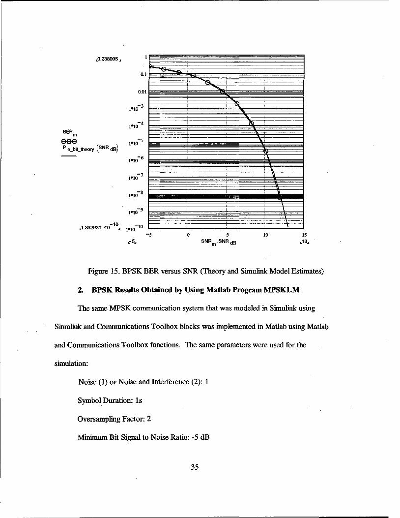
The estimates (obtained from the Simulink model) for the BPSK bit error probability are

shown in Figure 15 together with the theoretical BER versus the SNR.

34

L0.238095_.

I 0.1

....... !

0.01 --

1•10-3 ~

. -4 I

1•10 ·-m I

BERm ' :

eee 1•10-5 I " ; I

p e_biUheory (SNR dB)

1•10-6 i\ I

. . 1910-7 I i \\

1•10-8 \\

1•10-9 \

-10 ' L1.332931 ·10 .I 1•10-10 I \ I

-5 0 5 10 15 L-s .. SNRm,SNRdB L13 ..

Figure 15. BPSK BER versus SNR (Theory and Simulink Model Estimates)

2. BPSK Results Obtained by Using Matlab Program MPSKl.M

The same MPSK communication system that was modeled in Simulink using

Simulink and Communications Toolbox blocks was implemented in Matlab using Matlab

and Communications Toolbox functions. The same parameters were used for the

simulation:

Noise (1) or Noise and Intetference (2): 1

Symbol Duration: ls



35


Number of values for SNR: 10 or 18


Factor multiplying the error numbers: 2

Maximum size of the random integer arrays: 106

File name to save data: MATLAB_NOISE_2

The simulation output data were saved and visualized using . an auxiliary Mathcad script.

The theoretical bit error probability and the estimates obtained from the Matlab simulation

are shown in Figure 16 as functions of the signal-to-noise ratio SNR.

36

.. 0.285714 ..

BER m

e-e p e_bit_th(SNR dB) _

4 jt-----~----~---'+\--+-1i -1\.--------t

1910

I ' I

Figure 16. BPSK BER versus SNR (Theory and Matlab Model Estimates)

In this case, simulation results differ from theory. At closer inspection, one notices that

the curve for the estimates is similar to the theoretical curve but shifted to the right. Such

a shift corresponds to an SNR ''loss". Indeed, if the SNR for the theoretical curve is

reduced by 3 dB, the theoretical curve and the Matlab estimate match each other, as

shown in Figure 17. Therefore, we may conclude that the Simulink model gives very

accurate estimates for the bit error rate of BPSK with A WGN while the Matlab model

experiences a 3 dB SNR loss (compensating for this SNR loss again produces accurate

estimates). This seems to indicate a fundamental problem with the Communications

Toolbox.

37

~0.286715 ..

-7 7 ~613068 ·10 .. 1910-

0 5

SNRm,SNRdB

10

\

15 ~14 ..

Figure 17. BPSK BER versus SNR (Theory for SNR-3dB and Matlab for SNR)

B. QPSK BIT ERROR PROBABILITY ESTIMATES

1. QPSK Results for the Simulink Model

The Simulink model used for the BPSK is a general model that can be used for any

MPSK. Therefore, the same model was used for QPSK by selecting the number of phases

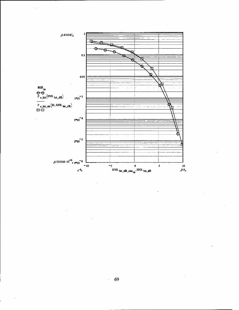
M (an input parameter) as four. The Simulink model results for the QPSK bit error

probability estimates are shown in Figure 18, together with the theoretical bit error

probability and its union bound given by [Ref.4]

SNRbit t1B

~bit ub(M,SNRbu dB)=~Q( log(M)2.10 10- .sin(~)) M-1 log(2) M

(25)

38

as functions of the bit signal-to-noise ratio SNRmt- We note that the estimates differ

somewhat from theory but that this difference diminishes as the bit SNR increases.

~0.410547~

- I ~

; -,... ~ 1 - I

~ 1 - i~ 0.1

·~ ..... I -I - '" '

i .......... Kl i I

I ~\_! I 0.01

' .... I

BER I I"( \

I I I \ \

I I

I \\ I I 1

m

e-e P e_bit(sNR bit_.m) 1•10-3

I

I I \I

I I \\

p e_bit_ub(M,SNR bit_dB)

&B I I I \\ I

I I . I I \\

! M

I ! \

I

I )

I I I I

-10 -s 0 5

SNR bit dB sim , SNR bit dB - - m -

Figure 18. QPSK BER versus SNR (Theory and Simulink Model Estimates)

2. QPSK Results Obtained by Using Madab Program MPSKl.M

The estimates for QPSK BER obtained using Matlab are shown in Figure 19,

together with the theoretical bit error probability and its union-bound estimate given by

Equation 25 as functions of the bit SNR.

39

~0.351719~ 1

. 0.1

O.oI

BER m

e-e P e_bit(sNR bit_clB) 1• 10-3


e-a

-6 -6 L5.}62801 ·10 ~ l'"JQ -10

~

I

I

I

I

i

'

i

I

I I

I I

-5

' I

! I

i I ..... t"'ol.~I ._. I

~ -I I

N" I ~ I I

~I ! i

' •n

I n ! '" i (\).

i ! "\, I

.. .. " I \\

! i ~

I I ' !

i i i

:

I I i

i I

0 5

SNR bit_dB_simm'SNR bit_dB

.. -IU.

\Y

\

\

10 ~10~

Figure 19. QPSK BER versus SNR (Theory and Matlab Model Estimates)

40

VI. SIMULATION VERIFICATION FOR BPSK AND QPSK WITH

ADDITIVE WHITE GAUSSIAN NOISE AND CO-CHANNEL INTERFERENCE

A. BPSK BIT ERROR PROBABILITY ESTIMATES

In the preceding chapter only additive white Gaussian noise (AWGN) was

considered for BPSK and QPSK simulations. In this chapter both AWGN and co-channel

interference are considered. A s~ond MPSK Mod block fed by an independent message

source generates the co-channel interference and is added to the sum of the signal and

noise. In the Simulink model and the Matlab program a range of signal-to-noise ratios

(SNR) and signal-to-interference ratios (SJR) are used to calculate the estimates of the bit

error probability as functions of SNR and SJR for both BPSK and QPSK. The results are

presented as families of curves, one with SNR as the variable and SJR as the parameter

and the other with SJR as the variable as SNR as the parameter.

The parameters for the BPSK simulations using both the Simulink model and

Matlab were:

Noise (1) or Noise and Interference (2): 2

The Number of Phases: 2

Symbol Duration: ls




Minimum Bit Signal to Interference Ratio: -5 dB

41

Maxim.um Bit Signal to Interference Ratio: 12 dB

Number of values for SNR: 10

Number of values for SJR: 10


Factor multiplying the number of error: 2

Maxim.um size of the random integer arrays: 106

File name to save data: NOISE&INTERFERENCE_2

The probabilities of bit error were saved as a BER matrix whose rows correspond

to constant values of SJR and whose columns correspond to constant values of SNR. The

selected ranges for SNR and SJR were from -5 dB to +12 dB. For each bit error

probability estimate (each matrix entry) at least 100 bit errors were observed. The

simulations ran until the error counter exceeded the minimum specified number of error, in

this case 100. Upon exceeding the minimum number of required bit errors, the simulation

was restarted for another combination of SNR and SJR (to create another BER matrix

entry). High values of SNR or SJR correspond to low noise and interference powers,

which in turn implies low probabilities of bit error. Therefore, the time required for the

simulation to produce at least 100 errors increases as the row and column indices (SJR

and SNR) increase, and the BER matrix entries in general decrease with increasing the

row and column indices.

For QPSK simulations the same parameter values were used as for BPSK except

for the number of phases M, which are four for QPSK. The BPSK simulation results were

plotted using auxiliary Mathcad programs plot_sim_noise&int2.mcd for the Simulink

42

model and plot_mat_noise&int2.mcd for Matlab program results. Similarly, the QPSK

simulation results were plotted using auxiliary Mathcad programs

plot_sim_noise&int4.mcd for Simulink model and plot_mat_noise&int4.mcd for the

Matlab program.

1. BPSK Results for the Simulink Model

The results for the bit error probability of BPSK with noise and co-channel

interference obtained using the Simulink model are shown in Figure 20 (BER versus SNR

with SJR as parameter) and in Figure 21 (BER versus SJR with SNR as parameter). The

increments for both SNR and SJR are 1.889 dB, starting from -5 dB.

43

~0.515.

P theo(sNR bit_dB)

BER m,O 0.1

~ BER

m,l e-B BER m,2 0.01

.. ~._f;:---BER m,3

e-e BER m,4 1910-3

BER m,5

BER m,6 1910-4

BER m,7

BER m,8 1910-5

BER m,9

-5

-·-- -~---- '''""" .. _.~~ -~~" . ~-·""'·"••0< ....... :"::"..""

1--------j----"""" ..... ~ ............... ~ . ........_ ...... ..._ """"""""

0

SJR=INFINITY ~ SJR=-5.00 dB e-B SJR=-3.11 dB --f~>"'4• SJR=-1.22 dB e-e SJR=0.67 dB

SJR=2.56dB SJR=4.44dB SJR=6.33 dB SJR=8.22dB SJR=l0.11 dB SJR=l2.00 dB

" '<'· ............... ·-.... ~ '

\ \\\r\ '\,

\ . \. \ \ \ \ \

\

\ \ .

\

5 10

SNR bit_dB,SNRm

Figure 20. BPSK BER versus SNR with SJR as Parameter (Simulink Model Estimates)

The "lowest" curve represents the theoretical bit error probability for BPSK with A WGN

only. The increase of BER with decreasing SJR is evident from Figure 20. The BPSK

probability of bit error as a function of SJR, with SNR as a parameter starting at -5 dB

and with 1.889-dB increments, is shown in Figure 21.

44

BER int_ only (sJR dB ,eps)

BERO,n

~ BERl,n

B-8 BER2,n -f>.,· BER3,n

e-e BER4,n

-5 -5 l ·10 1•10

-5 0 5 -5 SJR dB,SJRn

SNR=lNFINITY ~ SNR=-5.00 dB B-8 SNR=-3.11 dB -~»·- SNR=-1.22 dB e-e SNR=0.67 dB

SNR=2.56 dB SNR=4.44dB SNR=6.33 dB SNR=8.22dB SNR=l0.11 dB SNR=l2.00 dB

\

\ 10

Figure 21. BPSK BER versus SJR with SNR as Parameter (Simulink Model Estimates)

The "step function" represents the noise-free case, that is the case of co-channel

interference only. In such a case the probability of error is either 0.5 when the co-channel

interference power is larger than the signal power (negative SJR) or 0 when the signal

45

power is larger than the co-channel interference power. (In order to use the logarithmic

scale, the value of 0 for positive SJR has been replaced by a small non-zero value).

2. BPSK Results Obtained by Using Matlab Program MPSKl.M

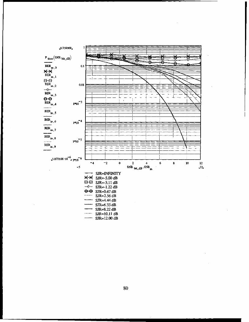
The results for the bit error probability of BPSK with noise and co-channel

interference obtained using Matlab program are shown in Figures 22 and 23 (BER versus

SNR with SJR as parameter starting at -5 dB and with 1.889 dB increments) and in

Figure 24 (BER versus SJR with SNR as parameter starting at -5 dB and with 1.889 dB

increments). Almost 3 dB difference can be noticed between simulation results and the

theoretical value. This difference was explained in the preceding section.

46

~0.338068~

-5

t-----t-----+---+--~i-...-----+-----=-·1~·-.•

0

SJR=INFINITY ~ SJR=-5.00 dB 8-B SJR=-3.11 dB -·¢' .. ·· SJR=-1.22 dB 0-e SJR=0.67 dB

SJR=2.56dB SJR=4.44dB SJR=6.33dB SJR=8.22dB SJR=l0.11 dB SJR=l2.00 dB

'

2 4 6

SNR bit_dB 'SNRm

i\

\

\

\

8 10 12

J2..

Figure 22. BPSK BER versus SNR with SJR as Parameter (Matlab Model Estimates)

Figure 23 shows the BPSK probability of bit error as a function of SJR, with SNR as a

parameter. Again, the difference between SNR curves is 1.889 dB as in SJR case. The

"step function" again represents the noise-free case, that is the case of co-channel

interference only.

47

.o.5.

BER int_only(sJR dB•eps)

BERO,n

~ BERl,n

e-s BER2,n

---<\)-

BER3,n

e-e BER4,n

-5

-./

.2.~::~.::::: --~:._,~ '=

-5 0

SNR=INFINITY ~ SNR=-5.00 dB B-B SNR=-3.11 dB ··-<;,...-- SNR=-1.22 dB 9-e SNR=0.67 dB

SNR=2.56dB SNR=4.44dB SNR=6.33 dB SNR=8.22dB SNR=l0.11 dB SNR=12.00 dB

5 SJR dB,SJRn

\

..... _ .......

'· ···-....

'\

'•

10 15 .12.

Figure 23. BPSK BER versus SJR with SNR as Parameter (Matlab Model Estimates)

48

B. QPSK BIT ERROR PROBABILITY ESTIMATES

1. QPSK Results for the Simulink Model

The results for the bit error probability of QPSK with noise and co-channel

interference obtained using the Simulink model are shown in Figure 24 (BER versus SNR

with SJR as parameter starting at -5 dB and with 1.889 dB increments) and in Figure 25

(BER versus SJR with SNR as parameter starting at -5 dB and with 1.889-dB

increments).

49

~0.497778~

p theo(SNR bit_dB)

BER m,O 0.1

~ BER

m,l

B--B BER

m,2 0.01

---"17--BER

m,3

e-e BER

m,4 l'"l.0-3

BER m,5

BER m,6 l'"l.0-4

BER m,7

BER m,8

t•to-5

BERm,9

-6 -6 ~5.162801 ·10 ~ t•to

-5

>---+---i--·-_-_-_-_,_+-_-_-_-=._~+:_~ ..... -......... --=--=-~~--... :..'•~~~·... .... ....

-2 0

SJR=INFINITY ~ SJR=-5.00 dB B--B SJR=-3.11 dB -(t,. ... h. SJR=-1.22 dB 0-e SJR=0.67 dB

SJR=2.56dB SJR=4.44dB SJR=6.33dB SJR=8.22dB SJR=l0.11 dB SJR=12.00 dB

2 4

SNR bit_dB ,SNRm

' \ '

\

6 8

·. ' \ \

10 12

~12..

Figure 24. QPSK BER versus SNR with SJR as Parameter (Simulink Model Estimates)

The "lowest" curve represents the theoretical bit error probability for QPSK with A WGN

only. The increase of BER with decreasing SJR (for positive SNR) is evident from Figure

24.

50

The QPSK probability of bit error as a function of SJR, with SNR as a parameter

starting at -5 dB and with 1.889-dB increments, is shown in Figure 25. The "step

function" again represents the noise-free case, that is the case of co-channel interference

only.

~0.5~

BER int_oniy(sJR dB,eps)

BERO,n

~ BERl,n

a-a BER2,n ·~t""

BER3,n

e-e BER4,n

BER5,n

I------~~ ~.--- ~ ~~ ~~ .,;;~:.>·::·~.: .. ·:~:·~---·- ::

0.1 ==3'.·· - . ->-------+-- '" ...... ........._ -- .... .....

-5 0

SNR==INFINITY ~ SNR==-5.00 dB B-B SNR==-3.11 dB ·-·<$... SNR==-1.22 dB 0-e SNR==0.67 dB

SNR==2.56 dB SNR==4.44dB SNR==6.33 dB SNR==8.22dB SNR==l0.11 dB SNR==12.00 dB

"\.. '>,., ...................... .

5 SJR dB,SJRn

' '

..,,, .. ,,

10

Figure 25. QPSK BER versus SJR with SNR as Parameter (Simulink: Model Estimates)

51

As can be seen in Figure 25, the curves for the bit error probability tend to the noise-free

step function as the SNR increases. Also, the curves for the negative SJR tend to 0.5,

meaning that the bit error probability is dominated by the interference for negative SJR, as

expected.

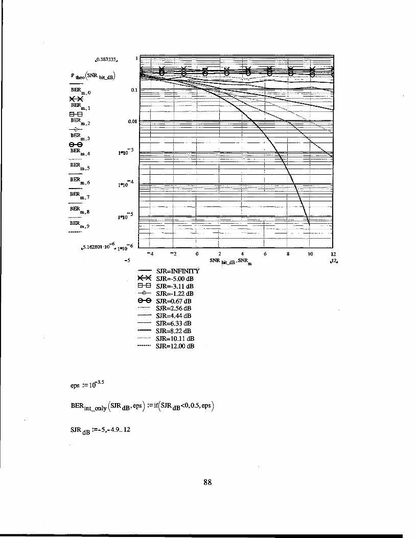
2. QPSK Results Obtained by Using Matlab Program MPSKl.M

The estimates for QPSK BER obtained using Matlab are shown in Figure 26

together with the theoretical bit error probability as a function of the bit SNR and with

SJR as parameter starting at -5 dB and with 1.889 dB increments. Comparing the BER

curves in Figures 24 and 26, we note that they differ slightly.

52

.o.383333~

P theo(sNR bit_.m)

-6 -6 .5.162801 ·10 ~ 1910

-5 0

SJR=INFINITY ~ SJR=-5.00 dB 8-B SJR=-3.11 dB --~,.... SJR=-1.22 dB 0-0 SJR=0.67 dB


\

' \

6 8

\

\

\

10 12

J2..

Figure 26. QPSK BER versus SNR with SJR as Parameter (Matlab Model Estimates)

The QPSK probability of bit error as a function of SJR, with SNR as a parameter

starting at -5 dB and with 1.889-dB increments, is shown in Figure 27. The "step

function" again represents the noise-free case, and the curves are seen to tend to the step

function as the SNR increases.

53

.o.5~


BERO,n

~ BERl,n

9-8 BER2,n

·-~>-··-

BER3,n

e-e ' '.

BER4,n \ \ "'"· \ \ ' \ •v.,

0.01 l==========t:::========t=======~t:, ="!i:~~======t

-5 0

SNR=INFINITY ~ SNR=-5.00 dB 9-8 SNR=-3.11 dB -~.,.- SNR=-1.22 dB 0-e SNR=0.67 dB

SNR=2.56 dB SNR=4.44dB SNR=6.33 dB SNR=8.22dB SNR=l0.11 dB SNR=12.00 dB

5 SJR dB,SJRn

' '•

\ \

' \ \. \ ......

\

10 15 .12..

Figure 27. QPSK BER versus SJR with SNR as Parameter (Matlab Model Estimates)

From these figures, we see that co-channel interference acts like noise. When co-channel

interference is high (SJR is low), the bit error probability is high and when it is low (SJR is

high) the bit error probability is low provided SNR is also high.

54

From an examination of Figures 26 and 27, we see that we can maintain P,, = 10-2

for SJR~ 12 dB when SNR;::: 8.22 dB. Up to a point, further increasing SNR allows SJR

to further decrease. A similar result is observed for BPSK, as can be seen from an

examination of Figures 20 through 23. Hence, the importance of AWGN on the effect of

co-channel interference cannot be overlooked.

55

VIL CONCLUSIONS AND RECOMMENDATIONS

A. CONCLUSIONS

The objective of this thesis was to model and simulate MPSK communication

systems in the presence of additive white Gaussian noise and co-channel interference. The

models were implemented as Simulink block-diagram models, using Simulink and

Communications Toolbox blocks, as well as Matlab programs, using Matlab and

specialized Communications Toolbox functions. Baseband equivalents of passband MPSK

systems were modeled using the complex envelope concept. The results for the bit error

probability were obtained for BPSK (2PSK) and QPSK ( 4PSK) modulation types with

additive white Gaussian noise only and with the sum of additive white Gaussian noise and

co-channel interference. Furthermore, the convergence (with increasing numbers of

"transmitted" symbols) of bit error probability estimates obtained by simulation to the

theoretical bit error probabilities has been verified for several cases of additive white

Gaussian noise with different variances.

The simulation results For A WGN only are in general very close to the theoretical

values and the estimates of the bit error rates converge to the theoretical values as the

numbers of transmitted symbols increase. However, it has been observed that the Matlab

model requires a 3 dB SNR correction for BPSK in noise case only. With this SNR

correction, the simulation results for the bit error probability match the theoretical results

and the results for the two implementations (SIMULINK and MATLAB) match each

57

other. The BPSK and QPSK are both sensitive to co-channel interference almost to the

same extent.

As a general rule, the sensitivity of both BPSK and QPSK to co-channel interference

can be reduced by increasing the SNR. Hence, the importance of A WGN on the effect of

co-channel interference cannot be overlooked. Of course, if the SJR becomes too small,

then performance is poor regardless of the SNR.

B. RECOMMENDATIONS

This research can be continued to include forward error correction and adjacent

channel interference in the developed models. Since only linear MPSK systems were

considered, a future study may address transmitter non-linearity. Theoretical derivation of

bit error probability can be obtained for MPSK with AWGN and interference which <;an be

either phase locked to the signal or with some given distribution (such as Uniform or

Gaussian) of the phase difference between the interference and the signal.

58

APPENDIX A. BATCH_RUN.M MATLAB PROGRAM FOR CONVERGENCE

TEST OF SIMULATION USING BPSK

% This program runs multiple simulations for convergence of simulink%

clear

num_symbols = input('Enter the number of symbols [1000]: '); if isempty(num_symbols), num_symbols = 1000; end

tic sim('mpsk7_z',num_symbols); disp('VAR 0.5 Done!') toe

tic sim('mpsk7_1',num_symbols); disp ('VAR 1 Done! ') toe

tic sim('mpsk7_2' ,num_symbols); disp ('VAR 2 Done!') toe

tic sim('mpsk7_4',nuffi_symbols); disp ('VAR 4 Done!') toe

tic sim('mpsk7_9' ,num_symbols); disp ('VAR 9 Done! ') toe

tic sim('mpsk7_16',num_symbols); disp ('VAR 16 Done!') toe

59

APPENDIX B. BER_PLOT.M MATLAB PROGRAM FOR PLOTTING THE

FIGURES OF THE SIMULATION FOR EACH VARIANCES

% This loads two files and plots the result

clear

num_bits = input('Enter the number of bits [1000]: ');

if isempty(num_bits), num_bits = 1000; end

load d:\errnuml.dat

load d:\bitnuml.dat

plot(bitnuml, errnuml ./ bitnuml, 'r-')

grid xlabel('Bit Number') ylabel('Bit Error Probability') title('Bit Error Probability for variance l')

[num_errors dummy] = size(errnuml); disp('noise variance=l') BER = num_errors I num_bits

61

APPENDIX C. PLOT_S™_NOISE2 MATHCAD PROGRAM FOR RESULTS OF

NOISE ONLY CASE BPSK USING S™ULINK MODEL

This program gives the probability of bit error vs. signal to noise ratio using outputs obtained from SIMULATION test for noise only BPSK.

BER := READPRN ( "h:\veys\simnoise2.ber"

SNR := READPRN ( "h:\veys\simnoise2.snr"

SNR := SNRT m := O .. rows ( SNR ) - 1

. 1 ( ( 1 P e_bit_theory (SN~ dB) := 2· 1 - erf ~ ·

SNR dB)) 2·10 10 SNR dB :=-5,-4.9 .. 13

LQ.238095.a

0.1

I

I -.. I I O.ot ----·

I

1•10-3 I I I \Jl. I

1•10-4 I ! I 1'\ - -

BERm -eee 1•10-5 I '\. I

p e_biUheory (SNR <E) 1•10-6 I i \

-1•10-7 I \\ I .. -···-··-· ---·-

---:. 1•10-8 \\ I

1•10"'.'9 I I I

-10 L1.332931 ·10 .a 1•10-10 I

. I

-5 0 5 10 15 L-5~ SNRm,SNRdB L13~

63

APPENDIX D. PLOT_MAT_NOISE2 MATIICAD PROGRAM FOR RESULTS

OF NOISE ONLY CASE BPSK USING MATLAB PROGRAM

This program gives the probability of bit error vs. signal to noise ratio using outputs obtained from MATLAB test for noise only BPSK.

BER:= READPRN( "h:\veys\matnoise2.ber" )

SNR := READPRN( ''h:\veys\matnoise2.snr" )

SNR:=SNRT

m:=O .. rows(SNR)- 1

\. . i \.

'! I

l\ I

1~07 •.__~~~~--~~~---'~~~~---~.....__\~~----· -s o s ro ~

SNRm,SNRdB

plot with 3 db error

65

I

\

0 10 15

plot 3 dB corrected

66

APPENDIX E. PLOT_S™_NOISE4 MATHCAD PROGRAM FOR RESULTS OF

NOISE ONLY CASE QPSK USING S™ULINK MODEL

This program gives the probability of bit error vs. signal to noise ratio using outputs obtained from SIMULATION test for noise only QPSK.

BER := READPRN ( "h:\veys\simnoise4.ber" )

SNR := READPRN ( "h:\veys\simnoise4.snr"

SNR:=SNRT m:=O .. rows(SNR)-1

BER :=.!.~·BER 2 M-1

SNR bit dB sim - - m :=SNR - 3

m

SNR bit dB) Q ..fM,SNR . ) :=Q 6 log(4M) ·IO 10 -

t\ b1t_dB M - 1 log( 2)

p e_biLQAM (M,SNRbit_dB) := li-~ -Q~M,SNRbiLdB) { 1-(1-~)-Q~M,SNRbit_dB)] . 4M

67

P (M SNR ) M -0 log(M) ·2·10SNRI:um ·sm· (~))

e bit ub , bit dB :=--- - - M-1 log(2) M

SNR bit

(e M SNR ) 10----W- log(M) ·cos(0) p ' ' bit := log(2)

L en(e,M,SNRbit) := l+erf(p(e,M,SNRbit))

( ) ·- ( ) p(e,M,SNR bi~z ( )

0 0,M,SNRbit .-p 8,M,SNRbit -e ·I: erf 8,M,SNRbit

SNR bit

-1010~ P0(8,M,SNRbit) :-e. Iog(Z) ·(-

1-+0(0,M,SNRbit))

2~ ~

p e_bit(M,SNRbit) :=~ l-

SNRbit_dB :=-9,-6.9 .. 10

1t

M

1t

M

68

BER m

.. 0.410547 ..

e-e P e_bit(sNR bit_dB)


B-B

-10

..-9 ..

I~~ !

i r-... ' : '- "' ' l j ""' l'\J :

I ~\I ' I

' ' I I -I M:' I i I \ \

I

I

I \\ I

I ~· i I \l

! \\ I

I ', I

I \

! I I ' I \

! i I

I I I i I \

I ;

I I

i. I

I I

! I ! !

-5 0 5 10

SNR bit_dB_simm,SNR bit_dB . ..9.9 ..

69

.-------------------------------------------

APPENDIX F. PLOT_MA T_NOISE4 MATIICAD PROGRAM FOR RESULTS

OF NOISE ONLY CASE QPSK USING MATLAB PROGRAM

This program gives the probability of bit error vs. signal to noise ratio using outputs obtained from MA'ILAB test for noise only QPSK.

BER:= READPRl'i( "h:\veys\matnoise4.ber" )

SNR :=READPRl'i( "h:\veys\matnoise4.snr" )

SNR:=SNRT

m:=O .. rows(SNR)- 4

SNR bit dB) Q JM,SNR . ) :=Q 6 log(~) ·lO 10 -

t\ b1t_dB M- 1 log(2)

p e_bit_QAM (M,SNRmum) := 1 +~ -0 ~M,SNRbit_dB) { 1-( 1- .k-)-0 ~M,SNRbiLdB) l ~

71

SNRbit_dB ) , M log(M) 10 . 1t

p e bit ub(M,SNRbit dB) ·=---0 ·2-10 -sm(-) - - - M - 1 \'I log( 2) M

SNR bit dB sim := SNR - - m m BER:= BER

SNR bit

( ) , -10- log(M)

p 9,M,SNRbit .= 10 -cos(9) ~ log(2)

( ) ,_ ( ) p(0,M,SNRbi~ 2

_( ) 0 0,M,SNRbit .-p 0,M,SNRbit -e -1: erf\ 0,M,SNRbit

• 1t

M

1t

•M

72

BER m

~0.351719~

e-e P e_bit(sNR bit_dB)


a-a

0.1

O.ot

-10

- I

!

I

I I

I I

I

I

I

I

i -5

...., ~

...... ~ ~

I

NKl !

! ~ I

I ~I ...

' "' ~·

i I m I '\, !

" .. I \\ I ~

I I ~ I

I I ' !

I DU

I 1.:11 I I \

i I \ I

! I

I I

i i

0 5

SNR bit dB sim , SNR bit dB - - m -

73

APPENDIX G. PLOT_SIM_NOISE&INT2 MATHCAD PROGRAM FOR

RESULTS OF NOISE AND INTERFERENCE CASE BPSK USING SIMULINK

MODEL

This program gives the probability of bit error vs. signal to noise ratio and probability of bit error vs.signal to jamming ratio using outputs obtained from SIMULATION test for BPSK.

BER := READPRN ( "h:\veys\simnoint2.ber"

SNR := READPRN ( "h:\veys\simnoint2.snr" )

SIR := READPRN ( "h:\veys\simnoint2.sjr"

m :=O .. rows ( SNR) - 1

n :=O .. rows (SIR)- 1

SNRdB :=-5 .. 12

75

.. o.515~

P tbeo(sNR bit_cm)

BER 5 m,

BER 8 m,

-6 -6 .. 3.872108 ·10 ~ 1910

-5 eps := 10

-..5

SJRdB :=-5,-4.9 .. 12

""iiii.'·-~.,~ .. -......... ~. I -

!

-5 0

SJR=INFINITY SJR=-5.00 dB SJR=-3.11 dB SJR=-1.22 dB SJR=0.67dB SJR=2.56dB SJR=4.44d.B SJR=6.33dB SJR=8.22d.B SJR=l0.11 dB SJR=12.00 dB

76

v :-v --c

I '\.'\ -, ', •••• ••••• '-'\. f \.

\ \ ...... ~ '\_ ' ·~ •. ( \ '-,

\

\

\ <. \

'~ \ \

I\ \ \

' '

\ I

\ I

\

10

\ \

' ' \

15 .. 12..

._0.515 ..

BER int_only ( SJR dB ' eps)

BER O,n

~ BER 1,n

e-a BER 2,n

-$BER 3,n

e-e BER4,n

BER5,n

BER6,n

BER 7,n

BER 8,n

BER9,n

' · .•. "': '

... ,; .. '' !\ I \ I \

I

0 5 -5 SJR dB ,SJR n

SNR=INFINITY ~ SNR=-5.00 dB 9-8 SNR=-3.11 dB --G- SNR=-1.22 dB 0-0 SNR=0.67 dB

SNR=256dB SNR=4.44dB SNR=6.33dB SNR=8.22dB SNR=l0.11 dB SNR=12.00 dB

77

... ·,_

'-;.,"·.

\ '

\

..... ........ ,..

I '";_,

I ···••· .•.

\\,

. ;

' I ,,

10

.........

·. .. · ..

15 ..12 ..

APPENDIX H. PLOT_MAT_NOISE&INT2 MAIBCAD PROGRAM FOR

RESULTS OF NOISE AND INTERFERENCE CASE BPSK USING MATLAB

PROGRAM

This program gives the probability of bit error vs. signal to noise ratio and probability of bit error vs.signal to jamming ratio using outputs obtained from MATLAB test for BPSK.

BER := READPRN ( "h:\veys\matnoint2.ber"

SNR := READPRN ( "h:\veys\matnoint2.snr" )

SJR :=READPRN ( "h:\veys\matnoint2.sjr"

SNR :=SNRT SJR :=SJRT

m :=O .. rows (SNR)- 1

n :=o .. rows (SJR)- 1

SNR dB :=-5 .. 12

79

.,0.338068 ..

P theo(sNR bit_dB)

BER m,0 0.1

~ BER

m,l ~ BERm,2 0.01

~ BER

m,3

e-e BER m,4 1910-3

BERm,5

BER m,6 1910-4

BERm,7

BER m,8

1910-s

BER m,9

-6 -6 ._3.872101MO .. 1910

-5

"' ---

I

0

SJR=INFINITY ~ SJR=-5.00 dB 8-B SJR=-3.11 dB -e-- SJR=-1.22 dB e-e SJR=0.67 dB


2 4

SNR bit_dB,SNRm

80

I

Lo'

[ """' -_J

1· .......... !-

~~~· ...... . ~( ..... ~ .......

! '\

'\ i

i\

6 8

-.... 1-.. ' .,., I • •• '

I"\.·.,··· ....

\

\ I

\I

10

·· ..

12 .,12,,

-35 eps :=10 ·

BERint_only (SJRdB,eps) :=if(SJRdB<0,0.5,eps)

SJRdB :=-5,-4.9 .. 12

BER int_on1y(SJR dB•eps)

BERO,n

~ BER.l,n

8-8 BER.2,n

---eB~,n e-e BER.4,n

BER.5,n

BER.6,n

B~,n

~ ... j

-----

0

SNR=INFlNITY *°* SNR=-5.00 dB 8-B SNR=-3.11 dB 4- SNR=-1.22 dB e-e SNR=0.67 dB

SNR=2.56dB SNR=4.44dB SNR=6.33 dB SNR=8.22dB SNR=l0.11 dB SNR=12.00 dB

81

I I

....... ! v

- ";:"

c:.. ;,<...

r _.

\. ·•.• "'- r "-..

···-.. I

\ \ I ····."-

\ .... ~ .....

I

'·

10 15

APPENDIX I. PLOT_SIM_NOISE&INT4 MATHCAD PROGRAM FOR

RESULTS OF NOISE AND INTERFERENCE CASE QPSK USING SIMULINK

MODEL

This program gives the probability of bit error vs. signal to noise ratio and probability of bit error vs.signal to jamming ratio using outputs obtained from SIMULATION test for QPSK.

M :=4

BER := READPRN ( "h:\veys\simnoint4.ber" )

SNR :=READPRN ("h:\veys\simnoint4.snr" . )

SJR := READPRN ( "h:\veys\simnoint4.sjr"

SNR :=SNR T - 3 SJR :=SJRT 1 M BER :=--·BER

2 M-1

m := 0 .. rows ( SNR) - 1

n := 0 .. rows ( SJR ) - 1

83

,.0.497TI8~

P theo(sNR bit_dB)

BER m,O

** BER m,1

e-s BER

m,2 --$---BER

m,3

e-e BER

m,4

BER m,5

BER m,6

BERm,7

BER m,8

BER m,9

-35 eps :=IO ·

0.1

0.01

1910-3

1910-4

1910-5

-5

I

!

-2 0

SJR=INFINITY ** SJR=-5.00 dB e-e SJR=-3.11 dB -$--- SJR=-1.22 dB 0-0 SJR=0.67 dB


2 4

SNR bit_dB 'SNR m

BERint_only (SJRdB,eps) :=if(SJRdB<0,0.5,eps)

SJRdB :=-5,-4.9 .. 12

84

\

i\

6 8

'J ··.. '

I '-.. ·•• •• ,_

I '•

\ I

\ I

\I

10 12 .. 12..

.. o.s ..

I I

I

BER int_on1y(sm dB'~)

BERO,n

** BERl,n

s-a BER2,n

-eBER3,n

.a-e BER4,n

BER5,n

BER6,n

''!--\ ··,······, ......... ~ 0.01 l=========:::t==========:::;:::'.'i;:::===':;:;::======:::::====:::I

\

-4 -4 HO 1910

-5 -5 0

SNR=INFINITY ** SNR=-5.00 dB 8-B SNR=-3.11 dB ~ SNR=-1.22 dB 0-0 SNR=0.67 dB

SNR=256dB SNR=4.44dB SNR=6.33dB SNR=8.22dB SNR=l0.11 dB SNR=12.00 dB

85

\

' ·• .. ,

'i· ..

\ i \. I

10 15 .. 12..

APPENDIX J. PLOT_MA T_NOISE&INT4 MA TH CAD PROGRAM FOR

RESULTS OF NOISE AND INTERFERENCE CASE QPSK USING MATLAB

PROGRAM

This program gives the probability of bit error vs. signal to noise ratio and probability of bit error vs.signal to jamming ratio using outputs obtained from MATLAB test for QPSK.

M :=4

BER := READPRN ( "h:\veys\matnoint4.ber" )

SNR := READPRN ( "h:\veys\matnoint4.snr" )

SJR :=READPRN ( "h:\veys\matnoint4.sjr"

m :=O .. rows (SNR)- 1

n :=O .. rows ( SJR)- 1

BER:=BER

87

.. o.383333,.

p tbeo(sNR bit_dB)

BERm,3

e-e BERm,4

BERm,5

BERm,6

0.01

1910-3

1910-4

-6 -6 .. 5.162801 ·10 .. 1910

-35 eps :=10 ·

-5

SJRdB :=-5,-4.9 .. 12

. ' Ml .... - '~.I

I

I

I

I

I I

i

I

-2 0

SJR=INFINITY ** SJR=-5.00 dB B-B SJR=-3.11 dB ~'- SJR=-1.22 dB e-e SJR=0.67 dB


'........_~ j.... i""'•· ....

'\.

:

2 4 6

SNR bit_dB 'SNR m

88

............ _

\.· I

i\

\

\

8 10

-

12 .. r2,,

~0.5~


-4 -4 MO 1910

-5 -5 0

SNR=INFINITY ** SNR=-5.00 dB e-B SNR=-3.11 dB --$- SNR=-1.22 dB &e SNR=0.67 dB

SNR=256d.B SNR=4.44d.B SNR=6.33 dB SNR=8.22d.B SNR=l0.11 dB SNR=l2.00 dB

89

5 SJR dB,SJRn

'.~, ....... i

" · ..

I\

10

\

APPENDIX K. PREPAPE.M MATLAB PROGRAM TO ENTER THE SYSTEM

PARAMETERS TO BE USED BY THE SIMUINK MODEL

%%% This prepares the data file for simulink runs clear

noise_only = menu(' Select: ', ... 'NOISE', ... 'NOISE and INTERFERENCE );

num_levels = input(Enter the number of frequencies M [2]: ); if isempty(num_levels), num_levels = 2; end

T_sym = input(Enter the symbol duration T [1]: ); if isempty(T_sym), T_sym = 1; end

oversampling = input( Enter the oversampling factor [2]: ); if isempty( oversampling), oversampling = 2; end

min_SNR = input(Enter the MIN Signal to Noise ratio[-5 dB]: ); if isempty(min_SNR), min_SNR :== -5; end

max_SNR = input(Enter the MAX Signal to Noise ratio [12 dB]: ); if isempty(max_SNR), max_SNR = 12; end if noise_only -= 1

min_SJR = input(Enter the MIN Signal to Interference ratio [-5 dB]: ); if isempty(min_SJR), min_SJR = -5; end max_SJR = input(Enter the MAX Signal to Interference ratio[12 dB]:);

if isempty(max_SJR), max_SJR = 12; end end if min_SNR == max_SNR

num_noise = 1; else

num_noise = input(Enter the number of values for SNR [10]: ); if isempty(num_noise), num_noise = 10; end

end

if noise_only -= 1 if min_SJR == max_SJR

num_jam= 1; else

num_jam = input(Enter the number of values for SJR [10]: ); if isempty(num_jam), num_jam = 10; end

end

91

else num_jam= 1;

end

min_errors = input(Enter the min number of errors acceptable [100]: ); if isempty(min_errors), min_errors = 100; end

error_factor = input(Enter the factor multiplying the number of errors [2]: ); if isempty(error_factor), error_factor = 2; end

initial_num_symbols = error_factor*min_errors;

max_randint = input(Enter the maximum size of the random integer arrays [10"6]: ); if isempty(max_randint), max_randint = 10"6; end

file_name = input(Enter the file name to save data [no ext]: ','s);

save sun_data

92

APPENDIX L. MPSK.M MATLAB PROGRAM TO START SIMULATION

%%% This runs MPSK co-channel interference with additive noise clear

load sun_ data % This loads all the input data

delta_t = T_sym/(2*oversampling) seeds = randint(3,1,1000); signal_seed = seeds(l); noise_seed = seeds(2); interf_seed = seeds(3); initial_num_symbols = error_factor*min_errors;

tic

if num_noise > 1 delta_SNR = (max_SNR - min_SNR) I (num_noise -1);

else delta_SNR = O;

end SNR = min_SNR + [O:num_noise - l]*delta_SNR; %noise_var_vect = T_sym/(2*delta_t) .* 10 ." (-SNR/10); noise_var_vect = 10 ." (-SNR/10);

if noise_only -= 1 ifnumjam> 1

delta_SJR = (max_SJR - min_SJR) I (numjam -1); else

delta_SJR = 0; end SJR = min_SJR + [O:numjam - l]*delta_SJR; interf_gain_vect = 10 ." (-SJR/20);

else SJR = - 100; % There is no Jamming so the SJR in dB is -infinity interf_gain_ vect = O;

end

BER = zeros(num_noise,numjam); total_symbols = initial_num_symbols; for noise_case = 1 :num_noise

noise_ var= noise_ var_ vect(noise_case ); for jam_case = l:numjam

enough_errors = 0;

93

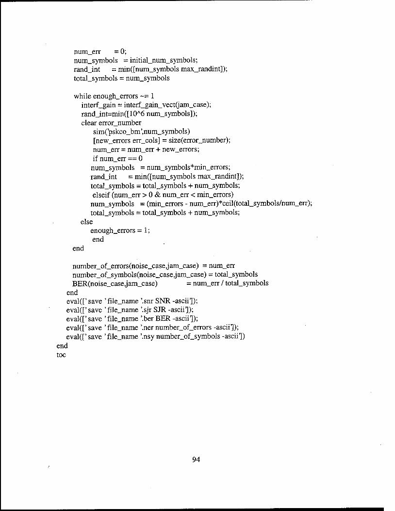
num_err = O; num_symbols = initial_num_symbols; rand_int = min([num_symbols max_randint]); total_symbols = num_symbols

while enough_errors -= 1 interf_gain = interf_gain_ vect(jam_case ); rand_int=min([ 10"6 num_symbols ]); clear error_number

sim('pskco_bm ',num_symbols) [new_errors err_cols] = size(error_number); num_err = num_err +new _errors; if num_err == 0

num_symbols = num_symbols*min_errors; rand_int = min([num_symbols max_randint]); total_symbols = total_symbols + num_symbols; elseif (num_err > 0 & num_err < min_errors)

num_symbols = (min_errors - num_err)*ceil(total_symbols/num_err); total_symbols = total_symbols + num_symbols;

else

end

enough_ errors = 1; end

number_of_errors(noise_case,jam_case) = num_err number_of_symbols(noise_case,jam_case) = total_symbols BER(noise_case,jam_case) = num_err I total_symbols

end eval([' save 'file_name '.snr SNR -ascii ]); eval([' save 'file_name '.sjr SJR -ascii ]); eval([' save 'file_name '.ber BER -ascii ]); eval([' save 'file_name '.ner number_of_errors -ascii]); eval([' save 'file_name '.nsy number_of_symbols -ascii ])

end toe

94

APPENDIX M. MPSKl.M MATLAB PROGRAM FOR USING MATLAB

PROGRAM OPTION VICE SIMULINK MODEL

%%%%%%%%%%%%%%%%%%%%%%%%%%%%% %%% Matlab Version forMPSK %%% %%% Dr. Jovan Lebatic %%% %%% June 14, 1998 %%% %%%%%%%%%%%%%%%%%%%%%%%%%%%%%

clear

%%%%%%%%%%%%%%%%%% %%% User Input %%% %%%%%%%%%%%%%%%%%%

j = sqrt(-1);

noise_only = menu(' Select: ', ... 'NOISE', ... 'NOISE and INTERFERENCE );M = input(Enter the number of phases

(power of 2) M [2]: ); if isempty(M), M = 2; end

T_sym = input(Enter the symbol duration T [1]: ); if isempty(T_sym), T_sym = 1; end

oversampling= input(Enter the oversampling factor [2]: ); if isempty( oversampling), oversampling = 2; end

min_SNR_bit = input(Enter the Minimum BIT Signal to Noise ratio in dB[-5 dB]:); if isempty(min_SNR_bit), min_SNR_bit = -5; end

max_SNR_bit = input(Enter the Maximum BIT Signal to Noise ratio in dB [+12 dB]:); if isempty(max_SNR_bit), max_SNR_bit = 12; end

if noise_only -= 1 min_SJR_bit = input(Enter the Minimum BIT Signal to Interference ratio in dB [-5

dB]:); if isempty(min_SJR_bit), min_SJR_bit = -5; end

max_SJR_bit = input(Enter the Maximum BIT Signal to Interference ratio in dB [+12dB]: );

if isempty(max_SJR_bit), max_SJR_bit = 12; end

95

end

if max_SNR_bit == min_SNR_bit num_noise = 1;

else num_noise = input(Enter the number of values for SNR [18]: );

if isempty(num_noise), num_noise = 10; end end

if noise_only -= 1 if min_SJR_bit == max_SJR_bit

numjam= 1; else

numjam = input(Enter the number of values for SJR [10]: ); if isempty(numjam), numjam = 10; end

end else

numjam= 1; end

min_errors = input(Enter the min number of errors acceptable [100]: ); if isempty(min_errors), min_errcirs = 100; end

error_factor = input(Enter the factor multiplying the number of errors [2]: ); if isempty(error_factor), error_factor = 2; end


max_randint = input(Enter the maximum size of the random integer arrays [10"6]: ); if isempty(max_randint), max_randint = 10"6; end

file_name = input(Enter the file name to save data [no ext]: ','s);

%%%%%%%%%%%%%%%%%%%%%%%%%%% %%% Parameters for MPSK %%% %%%%%%%%%%%%%%%%%%%%%%%%%%%

%%% Symbol Frequency %%% Fd = lff _sym;

%%% Sampling Frequency %%% Fs = oversampling*Fd;

%%% Sampling Interval %%% delta_t = 1/Fs;

96

%%% Seeds for Random Integers %%% seeds = randint(2,1,1000); signal_seed = seeds(l); interf_seed = seeds(2);


tic

%%% SNR Array%%% if num_noise > 1

delta_SNR_bit = (max_SNR_bit-min_SNR_bit) I (num_noise -1); else

delta_SNR_bit = O; end SNR_bit = min_SNR_bit + [O:num_noise - l]*delta_SNR_bit; · SNR_symbol = SNR_bit + 10*log10(log(M)/log(2));

%%% Noise Variance Array%%%% noise_var_vect = 10 .A (-SNR_symbol/10); %noise_var_vect = T_sym/ (2*delta_t) * 10 /\ (-SNR_symbol/10);

%%% SJR Array %%% if noise_only -= 1

if num_jam > 1 delta_SJR_bit = (max_SJR_bit - min_SJR_bit) I (num_jam -1);

else delta_SJR_bit = O;

end

SJR_bit = min_SJR_bit + [O:num_jam - l]*delta_SJR_bit; SJR_symbol = SJR_bit + 10*log10(log(M)/log(2)); interf_gain_vect = 10 .A (-SJR_symbol/20);

else

SJR_symbol = 100; SJR_bit = 100; % There is no Jamming so the SJR is large (infinity)

end

BER = zeros(num_noise,num_jam); total_symbols = initial_num_symbols;

97

%%%%%%%%%%%%%%%%%%%%%%%%%%%%%%%%%%%% %%% Noise and Interference Loops %%%

for noise_case = l:num_noise

noise_ var = noise_ var_ vect(noise_case );

for jam_case = l:num_jam

enough_errors = O; num_err =0; num_symbols = initial_num_symbols; rand_int = min([num_symbols max_randint]); total_symbols = num_symbols

while enough_errors -= 1

rand_int = min([l0"6 num_symbols]); input_sequence = randint(rand_int, 1,[0 M-1], signal_seed);

%%%%%%%%%%%%%%%%%%% %%% Modulation %%%% mod_MPSK = dmodce(input_sequence, Fd, Fs, 'psk', M);

%%%%%%%%%%%%%%%%%%%%%%%%%%%%%%% %%% Additive Gaussian Noise %%% randn('state ',sum(l OO*clock) ); complex_noise = randn(rand_int*oversampling, 1 )*sqrt(noise_ var); %randn('state',sum(200*clock)); %complex_noise = complex_noise +

j *randn(rand_int*oversampling, 1 )*sqrt( noise_ var);

mod_MPSK = mod_MPSK + complex_noise;

%%%%%%%%%%%%%%%%%%%%%%%%%%%%% %%% Additive Interference %%% if noise_ only-= 1

interf_gain = interf_gain_ vect(jam_case ); mod_MPSK = mod_MPSK + interf_gain*randint(rand_int*oversampling, 1,[0

M-1], interf_seed); end

%%%%%%%%%%%%%%%%%%%%

98

%%% Demodulation %%% demod_MPSK = ddemodce(mod_MPSK, Fd,Fs, 'psk',M);

%%%%%%%%%%%%%% %%% Errors %%%

[symbols_in_error dummy_col] = find(demod_MPSK- input_sequence); [new_errors dummy_col] = size(symbols_in_error); num_err = num_err + new _errors;

if num_err == 0 num_symbols = num_symbols*min_errors; rand_int = min([num_symbols max_randint]); . total_symbols = total_symbols + num_symbols; elseif (num_err > 0 & num_err < min_errors)

num_symbols = (min_errors - num_err)*ceil(total_symbols/num_err); total_symbols = total_symbols + num_symbols;

else enough_ errors = 1;

end

end

number_of_errors(noise_case,jam_case) = num_err number_of_symbols(noise_case,jam_case) = total_symbols BER(noise_case,jam_case) = 0.5 * M/(M-1) * num_err I total_symbols

end

eval([' save 'file_name '.snr SNR_bit -ascii 1); eval([' save 'file_name '.sjr SJR_bit -ascii 1); eval([' save 'file_name '.ber BER -ascii 1); eval([' save 'file_name '.ner number_ of_ errors -ascii 1); eval([' save 'file_name '.nsy number_of_symbols -ascii1);

end

toe

99

LIST OF REFERENCES

1. Communications Toolbox for Use with MATLAB and SIMULINK, The MATHWORKS Inc.

2. Hwei P.Hsu, Schaum's Outlines, Analog and Digital Communications, McGraw-Hill, 1993.

3. Bernard Sklar, Digital Communications Fundamental and Applications, Prentice Hall, New Jersey, 1988.

4. John Proakis, Digital Communications, McGraw-Hill, New York, 1995.

101

BIBLIOGRAPHY

1. Bernard Sklar, Digital Communications Fundamental and Applications, Prentice Hall, New Jersey, 1988.

2. John Proakis, Digital Communications, McGraw-Hill, New York, 1995.

3. I. A Glover & P. M.Grant, Digital Communications, Prentice Hall Europe, 1998.

4. Communications Toolbox for Use with MATLAB and SIMULIN.K, The MATHWORK.S Inc.

5. Hwei P.Hsu, Schaum's Outlines, Analog and Digital Communications, McGraw-Hill, 1993.

6. Dr. Jovan Lebaric, Notes for EC4550 (Digital Communications), Naval Postgraduate School, 1998 (unpublished).

103

INITIAL DISTRIBUTION LIST

No. Copies 1. Defense Technical Information Center .......................................................... 2

8725 John J. Kingman Rd., STE 0944 Fort Belvoir, VA 22060-6218

2. Dudley Knox Library ................................................................................... 2 Naval Postgraduate School 411 DyetRd. Monterey, CA 93943-5101

3. Chairman, Code EC ..................................................................................... 1 Department of Electrical and Computer Engineering Naval Postgraduate School Monterey, CA 93940-5121

4. Dr. Jovan Lebaric, Code EC/LB ................................................................... l Department of Electrical and Computer Engineering Naval Postgraduate School Monterey, CA 93940-5121

5. Dr. Clark Robertson, Code EC/RC .............................................................. 1 Department of Electrical and Computer Engineering Naval Postgraduate School Monterey, CA 93943-5121

6. Kara Kuvvetleri K.ligi MEBS. Bsk.ligi ......................................................... 1 Bakanliklar, Ankara, Turkey

7. Kara Kuvvetleri K.ligi Teknik ve Proje Yonetim Daire Bsk.ligi ................. 1 Bakanliklar, Ankara, Turkey

8. Kara Kuvvetleri K.ligi Kutuphanesi ........................................................•..... 1 Bakanliklar, Ankara, Turkey

9. Kara Harp Okulu K.ligi Kutuphanesi ............................................................ 1 Yenisehir, Ankara, Turkey

10. Veysel Erdogan ........................................................................................... 2 Ergenekon Mah. Kumkale Sok. No=27 /9 Yenimahalle, Ankara, Turkey 06210

105

a simulation of mpsk communications system performance in

Documents