A Simulation of Covered Call Strategy

Jiong Chen, Yu Xiang, Zhangpu Luo

May 14, 2014

Abstract Covered call is a trading strategy that is commonly used in stock market, which can be realized by shorting the call option while taking a long position at the underlying stock. This article analyze the performance of covered call by comparing BXM and S&P 500 then build up our own portfolio to simulate this strategy. The results of both methods agree in that: First, covered call can lower volatility and reduce uncertainty of the returns; Second, Covered call can provide cushions and generate more income while market goes down

1. Introduction

1.1 Covered Call Strategy Overview A covered call strategy is an income-generating strategy achieved by shorting the call option and longing the underlying stock at the same time. The goal here is to collect premium paid by the option buyer. If the stock price does not exceed the strike price, then the covered call strategy will outperform the equivalent long position. In this case, the long position in underlying stock is said to provide a “cover” since the shares are guaranteed to be able to deliver to the option buyer if the buyer decides to exercise. In short, investors who utilize covered call strategy give up the chance of unlimited capital gain for a higher probability of total return.

1.2 Applications and Illustration To be more explicit, we draw a simple straightforward chart below:

Here, the blue line is the payoff resulting from shorting a call option; the solid grey line is the payoff from longing the stock; and the top dotted line represents the net payoff with premium, which is higher than just longing the stock. Example: Pay 527.4 to long one share of Google stock today, and short 530 strike call, collect 10.6 premium from the call option sold. Net cost: 527.4 – 10.6 = 516.8 Scenario 1: stock price S > K, net return is capped at (530-527.4+10.6)/516.8=2.55% Scenario 2: stock price stayed flat, net return is 10.6/516.8=2.05% Scenario 3: stock price S < K, the investor is in the risk of losing money, however, the call premium collected will provide a cushion to the downside risk As we can see form the example above, we have the following possible outcomes:

Assume call strike > initial stock price, 1. If the stock stats flat, the call won’t be exercised, the strategy generates income from the

call premium. 2. If the stock price declines, the call won’t be exercised either. The strategy is in risk of loss

from long stock position, but the option premium acts as a cushion. 3. If the stock rises above the strike, call will be exercised. The strategy will lose the

potential gain from stock appreciation. The total return is capped.

2. Stock Covered Call Strategy Performance

2.1 Data selection and explanations In order to analyze the performance of covered call strategy, we choose the S&P 500 Index and COBE S&P 500 Buy Write Index (𝐵𝑋𝑀!") to make a comparison. The COBE S&P 500 Buy

Write Index (BXM) is a benchmark index designed to track the performance of a hypothetical buy-write strategy on the S&P 500 Index, it is a passive total return index based on (1) buying an S&P 500 stock index portfolio, and (2) selling the near-term S&P 500 Index “covered” call option. Therefore, we can regard BXM as the S&P 500 Stock Index after using the covered call strategy, then we can compare the performance of those two index in order to see what will happen after using the strategy. We choose the range of the data from 01/01/08 to 12/31/12 because there can be bear market and bull market during these days, therefore, we can see in more detailed how the strategy performs. In addition, we choose to use the adjusted stock price in order to take into account the effect of dividends.

2.2 Some statistics that will be used in comparison (1) Annualized Return

𝐴𝑅 = [ (1+ 𝑅!

!

!

)]!! − 1

Where 𝑅! is the annual return in 𝑖!! year (2) Standard Deviation

𝑆𝐷(𝑟!) =(𝑟! − 𝑟)!!

!!!

𝑛 − 1

Where 𝑟! is the daily return of a index and 𝑟 = !!

𝑟!!!!!

(3) 90 days rolling volatility for 1 day 𝑣𝑜𝑙!" = 𝑆𝐷(𝑟!)!"

Where 𝑆𝐷  (𝑟!)!" is the standard deviation of the daily returns in 90 days (4) Annualized Volatility

𝐴𝑉 = 1  𝑑𝑎𝑦  𝑉𝑜𝑙 ∗ 250

2.3 Comparison of the two indexes

2.3.1 Covered call can lower volatility and reduce uncertainty of the returns

We can use the formula above to calculate the 1-day volatility and annual volatility to compare how volatile those two indexes are. We plot the 1-day volatility and annual volatility for both of the index. (Figure 1)

Average

Volatility:

S&P 500

23.3%

BXM 17.4%

Covered call is almost 1/4 less volatile

Figure 1 As we can see from the plot above, the annual volatility of BXM is lower than that of S&P 500, which means by using covered call, we can reduce the uncertainty of the returns provided by the stock. To further explore this, we can also derive the histogram of the returns of those two indexes and see how they are distributed. (Figure 2)

Figure 2: The histogram returns of S&P 500 and BXM

We can see from the plot the returns of BXM is more concentrated in its center than the returns of S&P 500, which means we can say the probability of achieving the returns in the center is high and we can have more stable returns.

2.3.2 Covered call can provide cushions and generate more income while market goes down

We can firstly calculate the annual returns of S&P 500 Indexes and BXM then compare them.(Table 1 and Figure 3)

0  

0.1  

0.2  

0.3  

0.4  

0.5  

0.6  

0.7  

1/4/08   1/4/09   1/4/10   1/4/11   1/4/12  

1-­‐day  vol  for  S&P  

Annual  vol  for  S&P  

1-­‐day  vol  for  BXM  

Annual  vol  for  BXM  

Table 1: The Annual returns Annual return of S&P 500 Annual return of

BXM 2012 0.116776032 0.045949957 2011 -0.0112197 0.051246843 2010 0.110018623 0.052708771 2009 0.196716033 0.241621832 2008 -0.375846486 -0.280455502

Figure 3: The Annual Returns of year from 2008 to 2012

Figure 4:The returns and excess returns for S&P 500 and BXM

-­‐0.5  

-­‐0.4  

-­‐0.3  

-­‐0.2  

-­‐0.1  

0  

0.1  

0.2  

0.3  

2012   2011   2010   2009   2008  

annual  return  of  S&P  500   annual  return  of  BXM  

-­‐0.6  

-­‐0.4  

-­‐0.2  

0  

0.2  

0.4  

0.6  

0.8  

Bear  Market  

Bull  Market  Slight  Bull  Market  

Bull  Market   Bear  Market  

Bull  Market  

S&P  500  

BXM  

excess  return  

We can see from the table and plot above that in the year of 2008, 2009 and 2011, the covered call strategy can outperform the market. We can also see that during the year of 2008, it is a strong bear market and the year of 2009 is a slight bull market while in the year of 2011 the market is also a bear market. To test whether this guess is right or not, we calculate the returns for both S&P 500 and BXM for a continuous time from 2008 to 2012. In addition, we calculate the excess return of BXM for S&P 500. (Figure 4) We can see from Figure 4 that in the bear market, covered call strategy outperform the naked one since all the excess returns during the bear market is positive. In the slight bull market, the situation is the same. However, in the bull market, covered call will underperform. The reason why it can provide a cushion while the market goes down lies in how this strategy works. The stockholders can write an out-of-money or at-the-money call option and receive the option premium from the option buyers, so they have at least this part of the income. While in the bear market, the strike price is higher than current price and the current price will continue to fall. The option buyers will not exercise the option therefore stockholders still hold the stock and receive income from selling the call option. This part of income will provide a cushion to the downfall of the portfolio owned by stockholders. As a result, covered call strategy can outperform the market while in the bear market. The situation is the same when the market is in slight bull. In slight bull market, the stock price will have less change and probably stay at the current. Under this circumstance, the option buyers will have less chance to exercise the option thus the stockholders still can have the stock while receiving the premium.

3. Simulation of covered call on stock portfolio

3.1 Parameters and basic assumptions For the simplest form of covered call portfolio, one share of a certain stock and one short call option of this stock are involved. Hence we use the following marks to illustrate how this portfolio works. 𝑡: Starting time; 𝑇: Maturity time of the call option; 𝑆!: Stock price at time 𝑡; 𝑆!: Stock price at time 𝑇; 𝐾: Strike price of the call option; 𝐶: Price of the call option; 𝑟!: Risk free rate; σ: Implied volatility of the option that is used in B-S model to calculate the option price; At first we wanted to simulate a sequence of investments in a certain period of time and calculate the return in each stage. We dropped this idea because it was required to pick the right option

with the ‘best’ strike every time, which was beyond our capability. Instead, we turned to compute the returns of the portfolio that contained a stock and a short call with ‘gentle’ strike. This also helped us avoid many problems in tiny details like round-offs. Here are the basic assumptions we use to simply the model: 1. Ignore volume of the stock and option markets, which means we can buy as much as we want

for a certain stock or sell an option with certain strike; 2. There’s always a buyer, or a seller for a fair price. This means if we decide to sell the

stock( or exercise the option) in logical prices, we always succeed; 3. Trading is instant. This allows portfolio turns into cash instantly and vice versa; 4. Always pick stocks of the biggest company with best liquidity. Their stocks and options are

traded everyday so we don’t have trouble unifying the trading time of different stocks; 5. Use Black-Scholes model to compute American calls as an approximation. And do not

exercise options in the half way. With this assumption we can treat American options the same way with European ones;

6. Taxes are ignored and transaction fees be as cheap as 1.5 cents per share of stock. Suppose we have a covered call portfolio with parameters described in previous section. To build this portfolio with one share of stock and one short call, we need:

𝑆! − 𝐶 This is also the value at time  𝑡 of this portfolio. 𝐶 is computed by using B-S model with parameter 𝑆!,  𝐾,  𝑡,  𝑇,  𝑟! and σ. In time 𝑇, the value of this portfolio becomes:

final  value = 𝑆! , if  𝑆! < 𝐾𝐾, otherwise

With values of this portfolio at starting and ending time, we can calculate the return of if in this period.

3.2 Source of data and portfolio return Options data are gathered from WRDS and stocks from yahoo finance. Besides we take US 3 months treasury rate as risk free rate. So the risk free rate data are from US department of treasury’s website. For the stock shall be as liquid as possible, 8 of the largest companies in their fields are collected. The benchmark as a reflection of the market is S&P 500 index. The name list of those stocks is: AAPL, MSFT, WFC, CVX, XOM, JNJ, JPM, PFE. We are also aware of that the covered call strategy may perform well in bear markets. So the time ranges from Jan 01, 2008 to Jan 01, 2013. To reduce our work, we limit the maturity of options to approximately a month. Hence we only need to compute the returns once a month for each stock. A typical portfolio cycle is like this:

Call option starts on: Monday Jan 14,2008; Call option expire on: Saturday Feb 16, 2008; Since stocks are not traded on Saturday, we can take close price on Friday Feb 15 as 𝑆! to compute final value of the portfolio. For stocks and options are not traded in Sunday, the next investment cycle starts on Feb 19 and end in Mar 22. Now the return of the portfolio is calculated as:

return =

𝑆!𝑆! − 𝐶

, if  𝑆! < 𝐾

𝐾𝑆! − 𝐶

, otherwise

We need to deduce the transaction fees from the final income, hence:

return =

𝑆! − 0.015𝑆! − 𝐶

, if  𝑆! < 𝐾

𝐾 − 0.015𝑆! − 𝐶

, otherwise

3.3 Simulation results

We divide the simulation result into three groups. Single stock vs. Covered call

Return rate curve of stocks and covered call for MSFT and JPM are given below.

Figure 5: Return rate of MSFT stock and covered call from year 2008 to 2013

Figure 6: Return rate of JPM stock and covered call from year 2008 to 2013

These graphs show that covered calls reduced stock volatilities. Next step we annualize the return for each case to see how covered call performs.

Figure 7: Annual return rate of JPM&MSFT stock and covered call from year 2008 to 2013

Now we can see that the covered call helps to reduce losses in bear market and performs better than stocks when returns are close to zero.

S&P 500 vs. Overall covered calls

Now we turn to the portfolio of eight covered calls on eight stocks previously introduced, each with the same amount of money at the beginning. Hence the overall return rate can be calculated by averaging on the return rate of each covered call. One more question is needed to be answer before the calculation of portfolio return: which strike to pick. For example, there are 5 different historical calls of WFC on 14 Jan 2008 which expires on 16 Feb 2008 with diverse strike:

-­‐1  

-­‐0.5  

0  

0.5  

1  

1.5  

2  

year1   year2   year3   year4   year5  

JPM  stock  

MSFT  stock  

JPM  covered  call  

MSFT  covered  call  

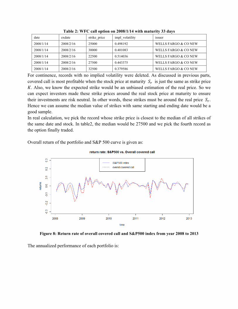
Table 2: WFC call option on 2008/1/14 with maturity 33 days date exdate strike_price impl_volatility issuer

2008/1/14 2008/2/16 25000 0.498192 WELLS FARGO & CO NEW

2008/1/14 2008/2/16 30000 0.401083 WELLS FARGO & CO NEW

2008/1/14 2008/2/16 22500 0.514036 WELLS FARGO & CO NEW

2008/1/14 2008/2/16 27500 0.443375 WELLS FARGO & CO NEW

2008/1/14 2008/2/16 32500 0.379586 WELLS FARGO & CO NEW

For continence, records with no implied volatility were deleted. As discussed in previous parts, covered call is most profitable when the stock price at maturity 𝑆! is just the same as strike price 𝐾. Also, we know the expected strike would be an unbiased estimation of the real price. So we can expect investors made these strike prices around the real stock price at maturity to ensure their investments are risk neutral. In other words, these strikes must be around the real price 𝑆!. Hence we can assume the median value of strikes with same starting and ending date would be a good sample. In real calculation, we pick the record whose strike price is closest to the median of all strikes of the same date and stock. In table2, the median would be 27500 and we pick the fourth record as the option finally traded. Overall return of the portfolio and S&P 500 curve is given as:

Figure 8: Return rate of overall covered call and S&P500 index from year 2008 to 2013

The annualized performance of each portfolio is:

Figure 9: Annual return rate of overall covered call and S&P500 index from year 2008 to 2013

4. Conclusion

From both the results of simulation and the analysis of BXM, we can have the same conclusion: First, Covered call can lower volatility and reduce uncertainty of the returns; Second, Covered call can provide cushions and generate more income while market goes down. Initially we aimed to do just simulation on covered calls but we had problem extracting data from WRDS database. So we turned to BXM as a replicate for the covered call. After settled the WRDS problem we simulated covered calls based on 10 stocks, MSFT, GOOG, AAPL, CVX, WMT, WFC, JNJ, PFE, JPM, XOM. The final result of covered call simulation just coincided with BXM and we knew we were on the right way.

Acknowledgements  

We  lost  one  team  member  in  halfway  of  this  project.  Christina  R  Rolle  had  to  go  back  home  for  family  affairs.  It  must  be  hard  to  make  such  decisions  in  the  final  period  of  a  semester.  We  just  hope  everything  be  fine  with  her.  It  was  totally  different  learning  theories  from  doing  simulations.  There  were  always  tons  of  details  needed   to  be  settled  such  as  what   to  choose  as   the   risk   free   rate  and  how  to  deal  with  options  records  without  implied  volatilities.  Hence   we   appreciate   professors   Smirnov,   TAs   and   graders   of   this   this   course.   The  homework  was   just  not   too  difficult   nor   too   easy.  We  also   learned  a   lot   from  completing  assignments  and  this  final  project.  

-­‐0.6  

-­‐0.4  

-­‐0.2  

0  

0.2  

0.4  

0.6  

1   2   3   4   5  

S&P500  

Overall  covered  call