a simplicial decomposition framework for large scale

Noname manuscript No.(will be inserted by the editor)

A simplicial decomposition framework for large scaleconvex quadratic programming

Enrico Bettiol · Lucas Letocart ·Francesco Rinaldi · Emiliano Traversi

Received: date / Accepted: date

Abstract In this paper, we analyze in depth a simplicial decomposition likealgorithmic framework for large scale convex quadratic programming. In par-ticular, we first propose two tailored strategies for handling the master prob-lem. Then, we describe a few techniques for speeding up the solution of thepricing problem. We report extensive numerical experiments on both real port-folio optimization and general quadratic programming problems showing theefficiency and robustness of the method when compared to Cplex.

Keywords Simplicial Decomposition · Large Scale Optimization · ConvexQuadratic Programming · Column Generation

Mathematics Subject Classification (2010) 65K05 · 90C06 · 90C30

E. BettiolLIPN, CNRS, (UMR7030), Universite Paris 13, Sorbonne Paris Cite,99 av. J. B. Clement, 93430 Villetaneuse, FranceE-mail: [email protected]

L. LetocartLIPN, CNRS, (UMR7030), Universite Paris 13, Sorbonne Paris Cite,99 av. J. B. Clement, 93430 Villetaneuse, FranceE-mail: [email protected]

F. RinaldiDipartimento di Matematica, Universita di PadovaVia Trieste, 63, 35121 Padua, ItalyTel.: +39-049-8271424E-mail: [email protected]

E. TraversiLIPN, CNRS, (UMR7030), Universite Paris 13, Sorbonne Paris Cite,99 av. J. B. Clement, 93430 Villetaneuse, FranceE-mail: [email protected]

2 Enrico Bettiol et al.

1 Introduction

We consider the following problem

min f(x) = x>Qx+ c>xs.t. aTi x = bi, i ∈ E

aTi x ≥ bi, i ∈ I(1)

with Q ∈ IRn×n, c ∈ IRn, ai ∈ IRn and bi ∈ IR, i ∈ E ∪ I.Moreover, we assume that the polyhedral set

X = {x ∈ IRn : aTi x = bi, i ∈ E} ∩ {x ∈ IRn : aTi x ≥ bi, i ∈ I}

is non-empty and bounded and that the Hessian matrix Q is positive semidef-inite. Among all possible problems of type (1), we are particularly interestedin the ones with the following additional properties:

– The number of constraints is considerably smaller than the number ofvariables in the problem, i.e. |E ∪ I| � n;

– the Hessian matrix Q is dense.

A significant number of large-scale problems, arising in many different fields(e.g. Communications, Statistics, Economics and Machine Learning), presenta structure similar to the one described above [4].

Solution methods for this class of problems can be mainly categorized intoeither interior point methods or active set methods [16]. In interior pointmethods, a sequence of parameterized barrier functions is (approximately)minimized using Newton’s method. The main computational burden is repre-sented by the calculation of the Newton system solution (used to get the searchdirection). Even if those methods are relatively recent (they started becomingpopulare in the 1990s), a large number of papers and books exist related tothem (see, e.g. [9, 15,22–24]).

In active set methods, at each iteration, a working set that estimates theset of active constraints at the solution is iteratively updated. This gives asubset of constraints to watch while searching the solution (which obviouslyreduces the complexity of our search in the end). Those methods, which havebeen widely used since the 1970s, turn out to be effective when dealing withsmall- and medium-sized problems. They usually guarantee efficient detectionof unboundedness and infeasibility (other than returning an accurate estimateof the optimal active set). An advantage of active set methods over interiorpoints is that they are well-suited for warmstarts, where a good estimate ofthe optimal active set or solution is used to initialize the algorithm. This turnsout to be extremely useful in applications where a sequence of QP problemsis solved, e.g., in a sequential quadratic programming method. A detailedoverview of active set methods can be found in [16].

In this paper, we develop a simplicial decomposition type approach (seee.g. [17, 20]) specifically tailored to tackle problems with the aforementionedfeatures. However, it is worth noting that the algorithm proposed can handle

A simplicial decomposition framework for convex quadratic programming 3

any problem of type (1) and can also be easily modified in order to deal withproblems having a general convex objective function. The reasons why we usethis kind of methods are very easy to understand. Simplicial decomposition likemethods, which are closely related to column generation approaches [17], areboth well suited to deal with large-scale problems and to be used in applica-tions where sequences of QPs need to be solved (since they can take advantageof warmstarts). Those tools can thus be fruitfully used in, e.g., Branch andPrice like schemes for convex quadratic integer programming.

The paper is organized as follows. In Section 2, we describe in depth theclassic simplicial decomposition framework. In Section 3, we present somestrategies to improve the efficiency of the framework itself. In Section 4, wereport our numerical experience. Finally, in Section 5, we draw some conclu-sions.

2 Simplicial Decomposition

Simplicial Decomposition (SD) represents a class of methods used for dealingwith large scale convex problems. It was first introduced by Holloway in [11]and then further studied in other papers like, e.g., [10, 19, 20]. A completeoverview of this kind of methods can be found in [17].

The method basically uses an iterative inner approximation of the feasibleset X. The method can be viewed as a special case of column generationapplied to a non linear problem (we refer the reader to [7] for an extensiveanalysis of such a method). In practice, the feasible set X is approximated withthe convex hull of an ever expanding finite set Xk = {x1, x2, . . . , xm} wherexi, i = 1, . . . , m are extreme points of X. We denote this set with conv(Xk):

conv(Xk) = {x | x =

m∑i=1

λixi,

m∑i=1

λi = 1, λi ≥ 0} (2)

At each iteration, it is possible to add new extreme points to Xk in such away that a function reduction is guaranteed when minimizing the objectivefunction over the convex hull of the new (enlarged) set of extreme points. Ifthe algorithm does not find at least one new point, the solution is optimal andthe algorithm terminates.

The use of the proposed method is particularly indicated when the follow-ing two conditions are satisfied:

1. Minimizing a linear function over X is much simpler than solving the orig-inal nonlinear problem;

2. Minimizing the original objective function over the convex hull of a rela-tively small set of extreme points is much simpler than solving the originalnonlinear problem (i.e. tailored algorithms can be used for tackling thespecific problem in our case).


First condition is needed due to the way a new extreme point is generated.Indeed, this new point is the solution of the following linear programmingproblem

min ∇f(xk)>(x− xk)s.t. x ∈ X (3)

where a linear approximation calculated at the last iterate xk (i.e. the solu-tion obtained by minimizing f over conv(Xk) ) is minimized over the originalfeasible set X.

Below, we report the detailed scheme related to the classical simplicialdecomposition algorithm [2,17,20] (see Algorithm 1). At a generic iteration kof the simplicial decomposition algorithm, given the set of extreme points Xk,we first minimize f over the set conv(Xk) (Step 1), thus obtaining the newiterate xk then, at Step 2, we generate an extreme point xk by solving thelinear program (5). Finally, at Step 3, we update Xk.

Algorithm 1 Simplicial Decomposition Algorithm

Initialization: Choose a starting set of extreme points X0.

For k = 1, 2, . . .

Step 1) Generate iterate xk by solving the master problem

min f(x)s.t. x ∈ conv(Xk)

(4)

Step 2) Generate an extreme point xk by solving the subproblem

min ∇f(xk)>(x− xk)s.t. x ∈ X (5)

Step 3) If ∇f(xk)>(x− xk) ≥ 0, Stop. Otherwise Set Xk+1 = Xk ∪ {xk}End For

Finite convergence of the method is stated in the following Proposition(see, e.g., [2, 20]):

Proposition 1 Simplicial Decomposition algorithm obtains a solution of Prob-lem (1) in a finite number of iterations.

In [20], a vertex dropping rule is also used to get rid of those vertices inXk whose weight is zero in the expression of the solution xk (Step 1). Thisdropping phase does not change the theoretical properties of the algorithm(finiteness still remains), but it can guarantee significant savings in terms ofCPU time since it keeps the dimensions of the master problem small.

3 Some strategies to improve the efficiency of a simplicialdecomposition framework

In this section, we discuss a few strategies that, once embedded in the simplicialdecomposition framework, can give a significant improvement of the perfor-


mances, especially when dealing with large scale quadratic problems with apolyhedral feasible set described by a small number of equations.

Firstly, we present and discuss two tailored strategies to efficiently solve themaster problem, which exploit the special structure of the generated simplices.Then, we present a couple of strategies for speeding up the solution of thepricing problem.

3.1 Strategies for efficiently solving the master problem

Here, we describe two different ways for solving the master problem. At first,we analyze an adaptive conjugate directions method that can be used fordealing with the minimization of a quadratic function over a simplex, then wedescribe another tool, based on a projected gradient method, that allows us toefficiently handle the more general problem of minimizing a convex functionover a simplex.

3.1.1 An adaptive conjugate directions based method for solving the master

Before describing the details related to the first method, we report a result(see e.g. [18]) for the conjugate directions method that will be useful to betterunderstand our algorithm.

Proposition 2 Conjugate directions method makes it possible to find the min-imum point of a convex quadratic function f(x) : IRn → IR, and the solutionof the problem is obtained after less than n steps.

At iteration k, the master problem we want to solve (Step 1 of the SD Algo-rithm) is the following:

min f(x) = x>Qx+ c>x

s.t. x =∑k−1i=1 λixi∑k−1

i=1 λi = 1λi ≥ 0,

(6)

where the set Xk = {x1, . . . , xk−1} represents the affine basis given by all thevertices generated in the previous iterations (that is we are assuming, for thesake of clarity, that all points generated so far are included in the set Xk: ifsome points, with zero weight, have been removed with the so-called vertexdropping rule, the method works as well). Inspired by the approach describedin [20], we developed a procedure that uses in an efficient way suitably chosensets of conjugate directions for solving the master. The main idea is tryingto reuse, as much as possible, the conjugate directions generated at previousiterations of the SD Algorithm.

In practice, we start from the solution of the master at iteration k − 1,namely xk−1, and consider the descent direction connecting this point withthe point generated by the subproblem at iteration k − 1, namely dk−1 =


xk−1 − xk−1 (we express it in terms of the new coordinates of problem (6)).Furthermore, we assume that a set of conjugate directions D = {d1, . . . , dk−2},also expressed in terms of the new coordinates of problem (6), is availablefrom previous iterations. We then use a Gram-Schmidt like procedure to turndirection dk−1 into a new direction dk−1 conjugate with respect to the setD. We use the basis B = [x1, . . . , xk] to express points xs = xk−1 and xt =xk−1 + dk−1 thus obtaining respectively points λs and λt. We hence intersectthe halfline emanating from xs (and passing by xt) with the boundary of thesimplex in (6) by solving the following problem:

max αs.t. (1− α)λs + αλt ≥ 0.

(7)

The solution of problem (7) can be directly written as

α∗ =

(maxi

λsi − λtiλsi

)−1

.

We finally define point λp = (1−α∗)λs+α∗λt and solve the following problem

minβ∈[0,1]

f(B[(1− β)λs + βλp]).

If the optimal value β∗ < 1 we get, by Proposition 2, an optimal solution forthe master. Otherwise, β∗ = 1 and we are on the boundary of the simplex. Inthis case, we just drop those vertices whose associated coordinates are equalto zero, and get a new smaller basis B. If B is a singleton, we can stop ourprocedure, otherwise we minimize f(x) in the new subspace defined by B.In order to get a new set of conjugate directions in the considered subspace,we use directions connecting point x∗ = Bλ∗ = B[(1 − β∗)λs + β∗λp] witheach vertex xj in B (that is dj = xj − xp) and then use a Gram-Schmidt likeprocedure to make them conjugate (we want to remark that all directions djneed to be expressed in terms of the new basis B). We report the algorithmicscheme below (see Algorithm 2).

Finite convergence of an SD scheme that uses Algorithm 2 for solving themaster can be obtained by using same arguments as in [20]. The proof isbased on the fact that our polyhedral feasible set contains a finite numberof simplices (whose vertices are extreme points of the feasible set). Since theinterior of each simplex has at most one relative minimum and the objectivefunction strictly decreases between two consecutive points xk and xk+1 (keepin mind that ∇f(xk)>(xk − xk) < 0), no simplex can recur. Now, observingthat at each iteration we get a new simplex, we have that the number ofiterations must be finite.

3.1.2 A fast gradient projection method for solving the master

The second approach is a Fast Gradient Projection Method (FGPM) andbelongs to the family of gradient projection approaches (see e.g. [3] for an


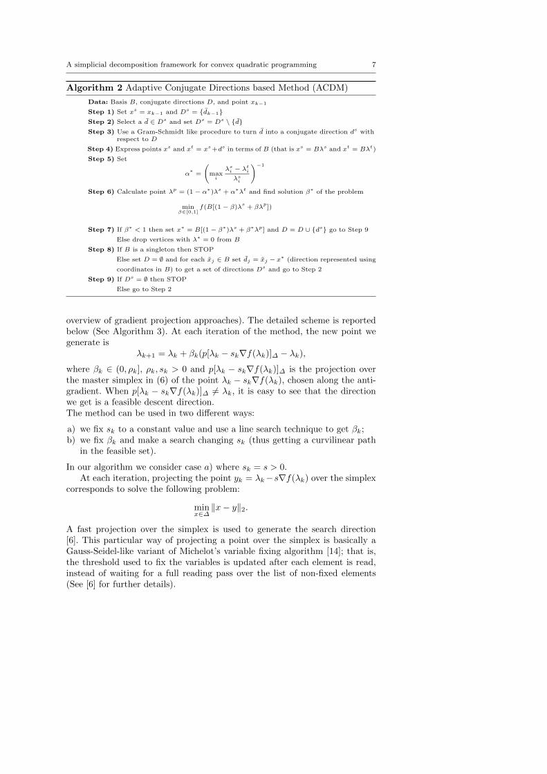
Algorithm 2 Adaptive Conjugate Directions based Method (ACDM)

Data: Basis B, conjugate directions D, and point xk−1

Step 1) Set xs = xk−1 and Ds = {dk−1}Step 2) Select a d ∈ Ds and set Ds = Ds \ {d}Step 3) Use a Gram-Schmidt like procedure to turn d into a conjugate direction ds with

respect to D

Step 4) Express points xs and xt = xs+ds in terms of B (that is xs = Bλs and xt = Bλt)

Step 5) Set

α∗

=

(maxi

λsi − λti

λsi

)−1

Step 6) Calculate point λp = (1− α∗)λs + α∗λt and find solution β∗ of the problem

minβ∈[0,1]

f(B[(1− β)λs

+ βλp])

Step 7) If β∗ < 1 then set x∗ = B[(1− β∗)λs + β∗λp] and D = D ∪ {ds} go to Step 9

Else drop vertices with λ∗ = 0 from B

Step 8) If B is a singleton then STOP

Else set D = ∅ and for each xj ∈ B set dj = xj − x∗ (direction represented using

coordinates in B) to get a set of directions Ds and go to Step 2

Step 9) If Ds = ∅ then STOP

Else go to Step 2

overview of gradient projection approaches). The detailed scheme is reportedbelow (See Algorithm 3). At each iteration of the method, the new point wegenerate is

λk+1 = λk + βk(p[λk − sk∇f(λk)]∆ − λk),

where βk ∈ (0, ρk], ρk, sk > 0 and p[λk − sk∇f(λk)]∆ is the projection overthe master simplex in (6) of the point λk − sk∇f(λk), chosen along the anti-gradient. When p[λk − sk∇f(λk)]∆ 6= λk, it is easy to see that the directionwe get is a feasible descent direction.The method can be used in two different ways:

a) we fix sk to a constant value and use a line search technique to get βk;b) we fix βk and make a search changing sk (thus getting a curvilinear path

in the feasible set).

In our algorithm we consider case a) where sk = s > 0.At each iteration, projecting the point yk = λk−s∇f(λk) over the simplex

corresponds to solve the following problem:

minx∈∆‖x− y‖2.

A fast projection over the simplex is used to generate the search direction[6]. This particular way of projecting a point over the simplex is basically aGauss-Seidel-like variant of Michelot’s variable fixing algorithm [14]; that is,the threshold used to fix the variables is updated after each element is read,instead of waiting for a full reading pass over the list of non-fixed elements(See [6] for further details).


Algorithm 3 Fast Gradient Projection Method (FGPM)

Data: Set point λ0 ∈ IRk−1, ρ0 ∈ [ρmin, ρmax] and a scalar value s > 0.

For k = 0, 1, . . .

Step 1) Generate point

λk = p[λk − s∇f(λk)]∆

Step 2) If λk = λk STOP; otherwise set dk = λk − λk

Step 3) Choose a stepsize βk ∈ (0, ρk] along dk and maximum stepsize ρk+1 by meansof a line search

Step 4) Set λk+1 = λk + βkdk

End For

A nonmonotone line search [?] combined with a spectral steplength choiceis then used at Step 3 (see [3] for further details) to speed up convergence. InAlgorithm 4 we report the detailed scheme of the line search. Convergence ofthe FPGM algorithm to a minimum follows from the theoretical results in [3].Therefore, the convergence of an SD method that uses FPGM to solve themaster problem directly follows from the results in the previous sections.

Algorithm 4 Non-monotone Armijo line-search (with spectral steplengthchoice)

0 Set δ ∈ (0, 1), γ1 ∈ (0, 12 ), M > 0

1 Updatefk = max

0≤i≤min{M,k}f(λk−i)

2 Set starting stepsize α = ρk and set j = 03 While f(λk + αdk) > fk + γ1 α∇f(λk)>dk4 set j = j + 1 and α = δjα.5 End While6 Set yk = ∇f(λk + αdk)−∇f(λk) and bk = αd>k yk7 If bk ≤ 0 set ρk+1 = ρmax else set ak = α2‖dk‖2 and

ρk+1 = min{ρmax,max{ρmin, ak/bk}}

In the FGPM Algorithm, we exploit the particular structure of the feasibleset in the master, thus getting a very fast algorithm in the end. We will seelater on that the FGPM based SD framework is even competitive with theACDM based one, when dealing with some specific quadratic instances.

3.2 Strategies for efficiently solving the pricing problem

Now we describe two different strategies for speeding up the solution of thepricing problem (also called subproblem). The first one is an early stopping


strategy that allows us to approximately solve the subproblem while guar-anteeing finite convergence. The second one is the use of suitably generatedinequalities (the so called shrinking cuts) that both cut away a part of thefeasible set and enable us to improve the quality of extreme points picked inthe pricing phase.

3.2.1 Early stopping strategy for the pricing

When we want to solve problem (1) using simplicial decomposition, efficientlyhandling the subproblem is, in some cases, crucial. Indeed, the total numberof extreme points needed to build up the final solution can be small for somereal-world problem, hence the total time spent to solve the master problems isnegligible when compared to the total time needed to solve subproblems. Thisis the reason why we may want to approximately solve subproblem (5) in sucha way that finite convergence is guaranteed (a similar idea was also suggestedin [2]). In order to do that, we simply need to generate an extreme point xksatisfying the following condition:

∇f(xk)>(xk − xk) ≤ −ε < 0, (8)

with ε > 0. Roughly speaking, we want to be sure that, at each iteration k,dk = xk − xk is a descent direction. Below, we report the detailed schemerelated to the simplicial decomposition algorithm with early stopping (seeAlgorithm 5).

Algorithm 5 Simplicial Decomposition with Early Stopping Strategy for theSubproblem

Initialization: Choose a starting set of extreme points X0

For k = 0, 1, . . .



Step 2) Generate an extreme point xk ∈ X such that

∇f(xk)>

(xk − xk) ≤ −ε < 0.

In case this is not possible, pick xk as the optimal solution of (5)

Step 3) If ∇f(xk)>(x− xk) ≥ 0, Stop. Otherwise set Xk+1 = Xk ∪ {xk}End For

At a generic iteration k we generate an extreme point xk by approximatelysolving the linear program (5). This is done in practice by stopping the algo-rithm used to solve problem (5) as soon as a solution satisfying constraint (8)is found. In case no solution satisfies the constraint, we simply pick the optimal


solution of (5) as the new vertex to be included in the simplex at the nextiteration.

Finite convergence of the method can be proved in this case as well:

Proposition 3 Simplicial decomposition with early stopping strategy for thesubproblem obtains a solution of Problem (1) in a finite number of iterations.

Proof. Extreme point xk, obtained approximately solving subproblem (5),can only satisfy one of the following conditions

1. ∇f(xk)>(xk − xk) ≥ 0, and subproblem (5) is solved to optimality. Hencewe get

minx∈X∇f(xk)>(x− xk) = ∇f(xk)>(xk − xk) ≥ 0,

that is necessary and sufficient optimality conditions are satisfied and xkminimizes f over the feasible set X;

2. ∇f(xk)>(xk−xk) < 0, whether the pricing problem is solved to optimalityor not, that is direction dk = xk − xk is descent direction and

xk /∈ conv(Xk). (9)

Indeed, since xk minimizes f over conv(Xk) it satisfies necessary and suf-ficient optimality conditions, that is ∇f(xk)>(x − xk) ≥ 0 for all x ∈conv(Xk).

From (9) we thus have xk /∈ Xk. Since our feasible set X has a finite numberof extreme points, case 2) occurs only a finite number of times, and case 1)will eventually occur. 2

3.2.2 Shrinking cuts

It is worth noticing that, at each iteration k, the objective function values ofthe subsequent iterates xk+1, xk+2, . . . , generated by the method will be notgreater than the objective function value obtained in xk, hence the followingcondition will be satisfied:

∇f(xk)>(x− xk) ≤ 0. (10)

This can be easily seen by taking into account convexity of f . Indeed, choosingtwo points x, y ∈ IRn, we have:

f(y) ≥ f(x) +∇f(x)>(y − x).

Thus, if ∇f(x)>(y − x) > 0, we get f(y) > f(x). Hence, f(y) ≤ f(x) implies∇f(x)>(y − x) ≤ 0.

We remark that all those vertices xi ∈ Xk not satisfying condition (10)have the related coefficient λi = 0 in the convex combination (2) giving themaster solution xk at iteration k. Proving this fact by contradiction is easy.Indeed, if we assume that a vertex xi is such that ∇f(xk)>(x − xk) > 0 and


the related λi 6= 0, then we can build a feasible descent direction in xk thuscontradicting its optimality.

We can take advantage of this property, as also briefly discussed in [2], byadding the cuts described above. The basic idea is the following: let xk be theoptimal point generated by the master at a generic iteration k, we can henceadd the following shrinking cut ck to the next pricing problems:

(ck) ∇f(xk)>(x− xk) ≤ 0.

More precisely, let {x1, . . . , xk} be the set of optimal points generated by themaster problems up to iteration k; then, for k > 0, we identify as Ck thepolyhedron defined by all the associated shrinking cuts as follows:

Ck = {x ∈ IRn : ∇f(xi)>(x− xi) ≤ 0, i = 0, . . . , k − 1}.

(We are assuming x0 := x0). Therefore, at Step 2, we generate an extremepoint xk by minimizing the linear function ∇f(xk)>(x − xk) over the poly-hedral set X ∩ Ck. Finally, at Step 3, if ∇f(xk)>(x− xk) ≥ 0, the algorithmstops, otherwise we update Xk by adding the point xk and Ck by adding thecut ∇f(xk)>(x− xk) ≤ 0.

Below, we report the detailed scheme related to the simplicial decomposi-tion algorithm with shrinking cuts (see Algorithm 6).

Algorithm 6 Simplicial Decomposition with Shrinking Cuts

Initialization: Choose a starting set of extreme points X0

For k = 0, 1, . . .



Step 2) Generate an extreme point xk by solving the subproblem

min ∇f(xk)>(x− xk)s.t. x ∈ X ∩ Ck

(11)

Step 3) If ∇f(xk)>(x− xk) ≥ 0, Stop. Otherwise set Xk+1 = Xk ∪ {xk} and

set Ck+1 = {x ∈ IRn : ∇f(xi)>(x− xi) ≤ 0, i = 0, . . . , k}

End For

In practice, we implemented the algorithm with the two following variants:

– At the end of Step 2, after the solution of the pricing problem, we removeall shrinking cuts that are not active. In this way we are sure to have apricing problem that is computationally tractable by keeping its size undercontrol.


– After a considerably large number of iterations k, no more shrinking cutsare added to the pricing. This is done to ensure the convergence of theAlgorithm.

Finite convergence of the method is stated in the following Proposition:

Proposition 4 Simplicial decomposition algorithm with shrinking cuts ob-tains a solution of Problem (1) in a finite number of iterations.

Proof. We first show that at each iteration the method gets a reduction off when suitable conditions are satisfied. Since at Step 2 we get an extremepoint xk by solving subproblem (11), if ∇f(xk)>(xk − xk) < 0, we have thatdk = xk − xk is a descent direction and there exists an αk ∈ (0, 1] such thatf(xk + αkdk) < f(xk). Since at iteration k + 1, when solving the masterproblem, we minimize f over the set conv(Xk+1) (including both xk and xk),then the minimizer xk+1 must be such that

f(xk+1) ≤ f(xk + αkdk) < f(xk).

Extreme point xk, obtained solving subproblem (11), can only satisfy one ofthe following conditions

1. ∇f(xk)>(xk − xk) ≥ 0. Hence we get

minx∈X∩Ck

∇f(xk)>(x− xk) = ∇f(xk)>(xk − xk) ≥ 0,

that is necessary and sufficient optimality conditions are satisfied and xkminimizes f over the feasible set X ∩ Ck. Furthermore, if x ∈ X \ Ck, weget that there exists a cut ci with i ∈ {0, . . . , k − 1} such that

∇f(xi)>(x− xi) > 0.

Then, by convexity of f , we get

f(x) ≥ f(xi) +∇f(xi)>(x− xi) > f(xi) > f(xk)

so xk minimizes f over X.2. ∇f(xk)>(xk − xk) < 0, that is direction dk = xk − xk is descent direction

andxk /∈ conv(Xk). (12)

Indeed, since xk minimizes f over conv(Xk) it satisfies necessary and suf-ficient optimality conditions, that is we have ∇f(xk)>(x− xk) ≥ 0 for allx ∈ conv(Xk).

Since from a certain iteration k on we do not add any further cut (notice thatwe can actually reduce cuts by removing the non-active ones), then case 2)occurs only a finite number of times. Thus case 1) will eventually occur. 2

Obviously, combining the Shrinking cuts with the Early Stopping strategycan be done (this is a part of what we actually do in practice) and finiteconvergence still holds for the simplicial decomposition framework.


4 Computational results

4.1 Instances description

We used two sets of instances as test-bed: portfolio instances and genericquadratic instances. They are both described in the following subsections.

4.1.1 Portfolio optimization problems

We consider the formulation for portfolio optimization problems proposed byMarkowitz in [13]. The instances used have a quadratic objective function (therisk, i.e. the portfolio return variance) and only two constraints: one giving alower bound µ on the expected return and one representing the so call “budget”constraint. The problem we want to solve is then described as follows

minx∈IRn

f(x) = x>Σx (13)

s.t. r>x ≥ µ,e>x = 1,

x ≥ 0,

where Σ ∈ IRn×n is the covariance matrix, r is the vector of the expectedreturns, and e is the n-dimensional vector of all ones.

We used data based on time series provided in [1] and [5]. Those data arerelated to sets of assets of dimension n = 226, 457, 476, 2196. The expectedreturn and the covariance matrix are calculated by the related estimators onthe time series related to the values of the assets.

In order to analyze the behavior of the algorithm on larger dimensionalproblems, we created additional instances using data series obtained by mod-ifying the existing ones. More precisely, we considered the set of data withn = 2196, and we generated bigger series by adding additional values to theoriginal ones: in order not to have a negligible correlation, we assumed that theadditional data have random values close to those of the other assets. For eachasset and for each time, we generate from 1 to 4 new values, thus obtaining4 new instances whose dimensions are multiples of 2196 (that is 4392, 6588,8784, 10980).

For each of these 8 instances, we chose 5 different thresholds for the ex-pected return: 0.006, 0.007, 0.008, 0.009, 0.01, we thus obtained 40 portfoliooptimization instances.


4.1.2 Generic quadratic problems

The second set of instances is of the form:

min f(x) = x>Qx+ c>x (14)

s. t. Ax ≥ b,l ≤x ≤ u.

with Q ∈ IRn×n symmetric and positive definite matrix, c ∈ IRn, A ∈ IRm×n,b ∈ IRm , l, u ∈ IRn and −∞ < l ≤ u < +∞. In particular, Q was built startingfrom its singular value decomposition using the following procedure:

– the n eigenvalues were chosen in such a way that they are all positive andequally distributed in the interval (0, 3];

– the n× n diagonal matrix S, containing these eigenvalues in its diagonal,was constructed;

– an orthogonal, n× n matrix U was supplied by the QR factorization of arandomly generated n× n square matrix;

– finally, the desired matrix Q was given by Q = USU>, so that it is sym-metric and its eigenvalues are exactly the ones we chose.

The coefficients of the linear part of the objective function were randomlyobtained, in a small range, between 0.05 and 0.4, in order to make the solutionof the problem quite sparse.

The m constraints (with m � n) were generated in two different ways:step-wise sparse constraints (S) or random dense ones (R). In the first case,for each constraint, the coefficients associated to short overlapping sequencesof consecutive variables were set equal to 1 and the rest equal to 0. Morespecifically, if m is the number of constraints and n is the number of columns,we defined s = 2 ∗ n/(m + 1) and all the coefficients of each i-th constraintare zero except for a sequence of s consecutive ones, starting at the position1 + (s/2) ∗ (i− 1). In the second case, each coefficient of the constraint matrixtakes a uniformly generated random value in the interval [0, 1]. The right-handside was generated in such a way to make all the problems feasible: for the step-wise constraints, the right hand side was set equal to f ∗s/n, with 0.4 ≤ f ≤ 1and for a given random constraint, the corresponding right-hand side b wasa convex combination of the minimum amin and the maximum amax of thecoefficients related to the constraint itself, that is b = 0.75∗amin+0.25∗amax.

Each class of constraints was then possibly combined with two additionaltype of constraints: a budget type constraint (b) e>x = 1, and a ”relaxed”budget type constraints (rb) slb ≤ e>x ≤ sub. Summarizing, we obtained sixdifferent classes of instances:

– S, instances with step-wise constraints only;– S-b, instances with both step-wise constraints and budget constraint;– S-rb, instances with both step-wise and relaxed budget constraints;– R, instances with dense random constraints only;– R-b, instances with both dense random constraints and budget constraint;


– R-rb, instances with both dense random and relaxed budget constraints.

For each class, we fixed n = 2000, 3000, . . . , 10000, while the number of bothstep-wise and dense random constraints m was chosen in two different ways:

1) m = 2, 22, 42 for each value of n;2) m = n/32, n/16, n/8, n/4, n/2 for each value of n.

In the first case, we then have problems with a small number of constraints,while, in the second case, we have problems with a large number of constraints.Finally, for each class and combination of n and m we randomly generatedfive instances. Hence, the total number of instances with a small number ofconstraints was 450 and the total number of instances with a large number ofconstraints was 750.

4.2 Preliminary tests

Here, we first describe the way we chose the Cplex optimizer for solving ourconvex quadratic instances. Then, we explain how we set the parameters in thedifferent algorithms used to solve the master problem in the SD framework.

4.2.1 Choice of the Cplex optimizer

As already mentioned, we decided to benchmark our algorithm against Cplexversion 12.6.2 (see [12] for further details). The optimizers that can be usedin Cplex for solving convex quadratic continuous problems are the following:primal simplex, dual simplex, network simplex, barrier, sifting and concurrent.The aim of our first test was to identify, among the 6 different options, whichis the most efficient for solving instances with a dense Q and n� m.

In Table 1, we present the results concerning instances with 42 constraintsand three different dimensions n: 2000, 4000 and 6000. We chose problemswith a small number of constraints in order to be sure to pick the best Cplexoptimizer for those problems where the SD framework is supposed to givevery good performances. For a fixed n, three different instances were solvedof all six problem types. So, each entry of Table 1 represents the averagescomputing times over 18 instances. A time limit of 1000 seconds was imposedand in brackets we report (if any) the number of instances that reached thetime limit.

n Default Primal Dual Network Barrier Sifting Concurrent

2000 72.2 1.6 1.6 1.6 84.2 2.0 89.04000 641.8 (2) 12.7 13.9 13.9 618.0 (2) 11.5 689.4 (2)6000 1000.0 (18) 31.5 30.7 30.5 1000.0 (18) 26.3 1000.0 (18)

Table 1 Comparison among the different Cplex optimizers


The table clearly shows that the default optimizer, the barrier and theconcurrent methods give poor performances when dealing with the quadraticprograms we previously described. On the other side, the simplex type al-gorithms and the sifting algorithm seem to be very fast for those instances.In particular, sifting gives the overall best performance. Taking into accountthese results, we decided to use the Cplex sifting optimizer as the baselinemethod in our experiments. It is worth noticing that the sifting algorithm isspecifically conceived by Cplex to deal with problems with n� m, represent-ing an additional reason for comparing our algorithmic framework against thisspecific Cplex optimizer.

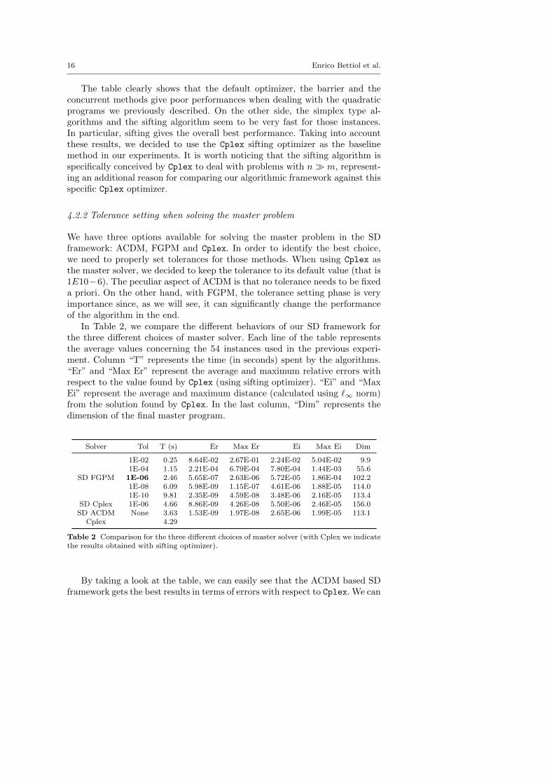
4.2.2 Tolerance setting when solving the master problem

We have three options available for solving the master problem in the SDframework: ACDM, FGPM and Cplex. In order to identify the best choice,we need to properly set tolerances for those methods. When using Cplex asthe master solver, we decided to keep the tolerance to its default value (that is1E10−6). The peculiar aspect of ACDM is that no tolerance needs to be fixeda priori. On the other hand, with FGPM, the tolerance setting phase is veryimportance since, as we will see, it can significantly change the performanceof the algorithm in the end.

In Table 2, we compare the different behaviors of our SD framework forthe three different choices of master solver. Each line of the table representsthe average values concerning the 54 instances used in the previous experi-ment. Column “T” represents the time (in seconds) spent by the algorithms.“Er” and “Max Er” represent the average and maximum relative errors withrespect to the value found by Cplex (using sifting optimizer). “Ei” and “MaxEi” represent the average and maximum distance (calculated using `∞ norm)from the solution found by Cplex. In the last column, “Dim” represents thedimension of the final master program.

Solver Tol T (s) Er Max Er Ei Max Ei Dim

SD FGPM

1E-02 0.25 8.64E-02 2.67E-01 2.24E-02 5.04E-02 9.91E-04 1.15 2.21E-04 6.79E-04 7.80E-04 1.44E-03 55.61E-06 2.46 5.65E-07 2.63E-06 5.72E-05 1.86E-04 102.21E-08 6.09 5.98E-09 1.15E-07 4.61E-06 1.88E-05 114.01E-10 9.81 2.35E-09 4.59E-08 3.48E-06 2.16E-05 113.4

SD Cplex 1E-06 4.66 8.86E-09 4.26E-08 5.50E-06 2.46E-05 156.0SD ACDM None 3.63 1.53E-09 1.97E-08 2.65E-06 1.99E-05 113.1

Cplex 4.29

Table 2 Comparison for the three different choices of master solver (with Cplex we indicatethe results obtained with sifting optimizer).

By taking a look at the table, we can easily see that the ACDM based SDframework gets the best results in terms of errors with respect to Cplex. We can


also see that the performance of the FGPM based one really changes dependingon the tolerance chosen. If we want to get for FGPM the same errors as ACDM,we need to set the tolerance to very low values, thus considerably slowing downthe algorithm. In the end, we decided to use a tolerance of 10E−6 for FGPM,which gives a good trade-off between computational time and accuracy. Thismeans anyway that we gave up precision to keep the algorithm fast with respectto ACDM.

4.3 Numerical results related to the complete testbed

Now, we analyze the performances of our SD framework when choosing differ-ent options for both solving the master and the pricing problem. Summarizing,we used three different methods for solving the master: Cplex, ACDM andFGPM. As for the pricing problems, we considered the use of the Early stop-ping (E) technique described in Section 3.2.1 and the Shrinking cuts (Cuts),described in Section 3.2.2. A further option we used in the SD framework isthe use of the LP sifting optimizer in the solution of the pricing problem in-stead of the standard one. We also notice that, in order to save CPU time, thevertex dropping rule described in Section 2 was always used in the framework.Summing up, for each choice of the master solver, we compared 8 different setsof options related to the pricing solver, indicated as follows:• Default (D) • Sifting (Sif)• Cuts (C) • Sifting+Cuts (Sif-C)• Early stopping (E) • Sifting+Early stopping (Sif-E)• Cuts+Early stopping (CE) • Sifting+Cuts+Early stopping (Sif-CE)

4.3.1 Portfolio optimization instances

Firstly, we tested the framework on the portfolio optimization instances. Forthe largest values of n, that is n > 2000, in Figure 1, we show the performanceprofiles related to the framework with the three different master solvers andthe sifting Cplex optimizer. We produced the performance profiles accordingto [8] and using the software Mathematica version 10.2 (see [21] for furtherdetails). For each SD method, the best pricing option was considered. We caneasily notice that the best choice in terms of master solver is ACDM.

In Figure 2, we report the performance profiles related to the best mastersolver (that is ACDM) for the different pricing options. As we can see, thebest option for the pricing is Sifting + Early Stopping.

4.3.2 Generic quadratic instances

Small number of constraints (GS) We first analyze the results related to thegeneric quadratic problems with a small number of constraints. The perfor-mance profiles reported in Figures 3 and 4 are related to all classes of con-straints described before.


2 3 4 5 6 7 8 9 10

0.2

0.4

0.6

0.8

1.0

SD Cplex

SD ACDM

SD FGPM

Cplex

Fig. 1 Performance profiles for Portfolio instances - master solvers.

2 3 4 5 6 7 8 9 10

0.2

0.4

0.6

0.8

1.0Default

Cuts

Early Stopping

Cuts+Early Stopping

Sifting

Sifting+Cuts

Sifting + Early Stopping

Sifting+Cuts+Early Stopping

Cplex

Fig. 2 Performance profiles for Portfolio instances - pricing options (SD ACDM).

2 3 4 5 6 7 8 9 10

0.2

0.4

0.6

0.8

1.0

SD Cplex

SD ACDM

SD FGPM

Cplex

Fig. 3 Performance profile for GS instances - master solvers.

Similarly to the results on portfolio instances, ACDM represents the bestchoice for solving the master; sifting is the best pricing option for ACDM,whose performance does not change a lot with the addition of the Early stop-ping strategy.


2 3 4 5 6 7 8 9 10

0.2

0.4

0.6

0.8

1.0Default

Cuts

Early Stopping

Cuts+Early Stopping

Sifting

Sifting+Cuts



Cplex

Fig. 4 Performance profile for GS instances - pricing options (SD ACDM).

Large number of constraints (GL) Here, we analyze the results obtained forinstances with a larger number of constraints. We need to keep in mind, any-way, that our SD framework works well only when the number of constraintsis significantly smaller than the number of variables.

Analogously as before, in Figures 5 and 6, we analyze the performances ofthe framework for the different choices of master solvers and pricing options.The results are compared using performance profiles (we consider all types ofconstraints in the analysis).

2 3 4 5 6 7 8 9 10

0.2

0.4

0.6

0.8

1.0

SD Cplex

SD ACDM

SD FGPM

Cplex

Fig. 5 Performance profile for GL instances - master solvers.

In this case something different happens:

– Cplex, SD ACDM and SD Cplex, reach the time limit on some instances;– the best master solver now is clearly FGPM. SD ACDM and SD Cplex are

even worse than Cplex in terms of efficiency, but are more robust.– the best pricing option is Sifting + Cuts. So, the use of this type of cuts,

which was ineffective when dealing with portfolio and GS instances, sig-nificantly improves the performance here. We get the same improvementwhen using the other master solvers too.


2 3 4 5 6 7 8 9 10

0.2

0.4

0.6

0.8

1.0

Default

Cuts

Early Stopping

Cuts+Early Stopping

Sifting

Sifting+Cuts



Cplex

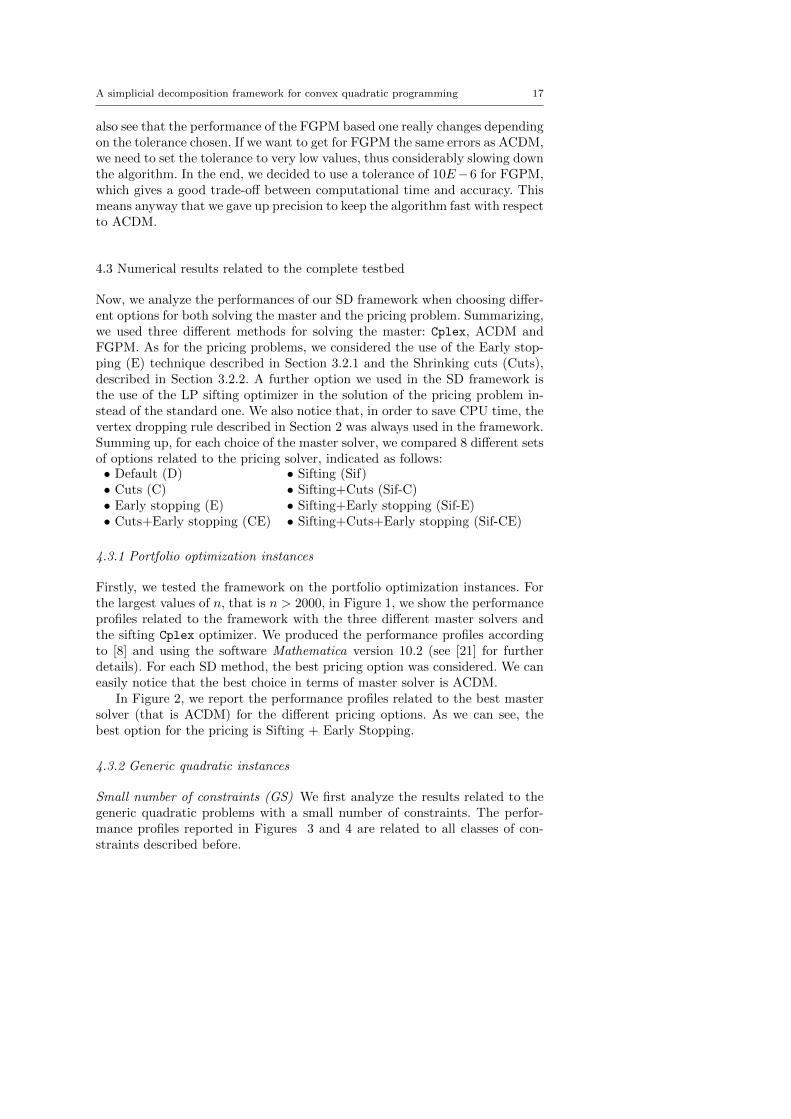
Fig. 6 Performance profile for GL instances - pricing options (SD FGPM).

As we said, some of the algorithms did not solve all the instances withinthe time limit of 1000 seconds. In particular, 122 instances out of 750 werenot solved by Cplex, only 8 by SD Cplex and 4 by SD ACDM (both with theSifting + Cuts option); SD FGPM (with the Sifting + Cuts option), on theother side, solved all the instances within the time limit.

The biggest difference with respect to the previous results is that now theperformance profiles of SD FGPM are better than those obtained using theother methods (and, in particular, better than SD ACDM, which was thebest one so far). The reason why this happens will become clearer later on(see Section 4.5), when an in-depth analysis of the results will be shown. Weanyway need to keep in mind that SD ACDM usually gives better solutions interms of errors when compared with SD FGPM.

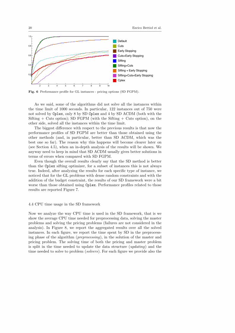
Even though the overall results clearly say that the SD method is betterthan the Cplex sifting optimizer, for a subset of instances this is not alwaystrue. Indeed, after analyzing the results for each specific type of instance, wenoticed that for the GL problems with dense random constraints and with theaddition of the budget constraint, the results of our SD framework were a bitworse than those obtained using Cplex. Performance profiles related to thoseresults are reported Figure 7.

4.4 CPU time usage in the SD framework

Now we analyze the way CPU time is used in the SD framework, that is weshow the average CPU time needed for preprocessing data, solving the masterproblems and solving the pricing problems (failures are not considered in theanalysis). In Figure 8, we report the aggregated results over all the solvedinstances. In each figure, we report the time spent by SD in the preprocess-ing phase of the algorithm (preprocessing), in the solution of the master andpricing problem. The solving time of both the pricing and master problemis split in the time needed to update the data structure (updating) and thetime needed to solve to problem (solvers). For each figure we provide also the


2 3 4 5 6 7 8 9 10

0.2

0.4

0.6

0.8

1.0

SD Cplex

SD ACDM

SD FGPM

Cplex

Fig. 7 Performance profile for GL instances (Rb constraints).

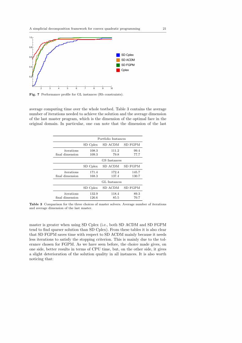
average computing time over the whole testbed. Table 3 contains the averagenumber of iterations needed to achieve the solution and the average dimensionof the last master program, which is the dimension of the optimal face in theoriginal domain. In particular, one can note that the dimension of the last

Portfolio Instances

SD Cplex SD ACDM SD FGPM

iterations 108.3 111.2 99.4final dimension 109.3 79.8 77.7

GS Instances



GL Instances



Table 3 Comparison for the three choices of master solvers. Average number of iterationsand average dimension of the last master.

master is greater when using SD Cplex (i.e., both SD ACDM and SD FGPMtend to find sparser solution than SD Cplex). From these tables it is also clearthat SD FGPM saves time with respect to SD ACDM mainly because it needsless iterations to satisfy the stopping criterion. This is mainly due to the tol-erance chosen for FGPM. As we have seen before, the choice made gives, onone side, better results in terms of CPU time, but, on the other side, it givesa slight deterioration of the solution quality in all instances. It is also worthnoticing that:


PreprocessingMaster updatingMaster solvingPricing updatingPricing solving

(a) SD Cplex. Average CPU Time = 27.5 s


(b) SD ACDM. Average CPU Time = 19.6 s


(c) SD FGPM. Average CPU Time = 11.3 s

Fig. 8 CPU time pie charts (Cplex Average CPU time = 39.8 s).


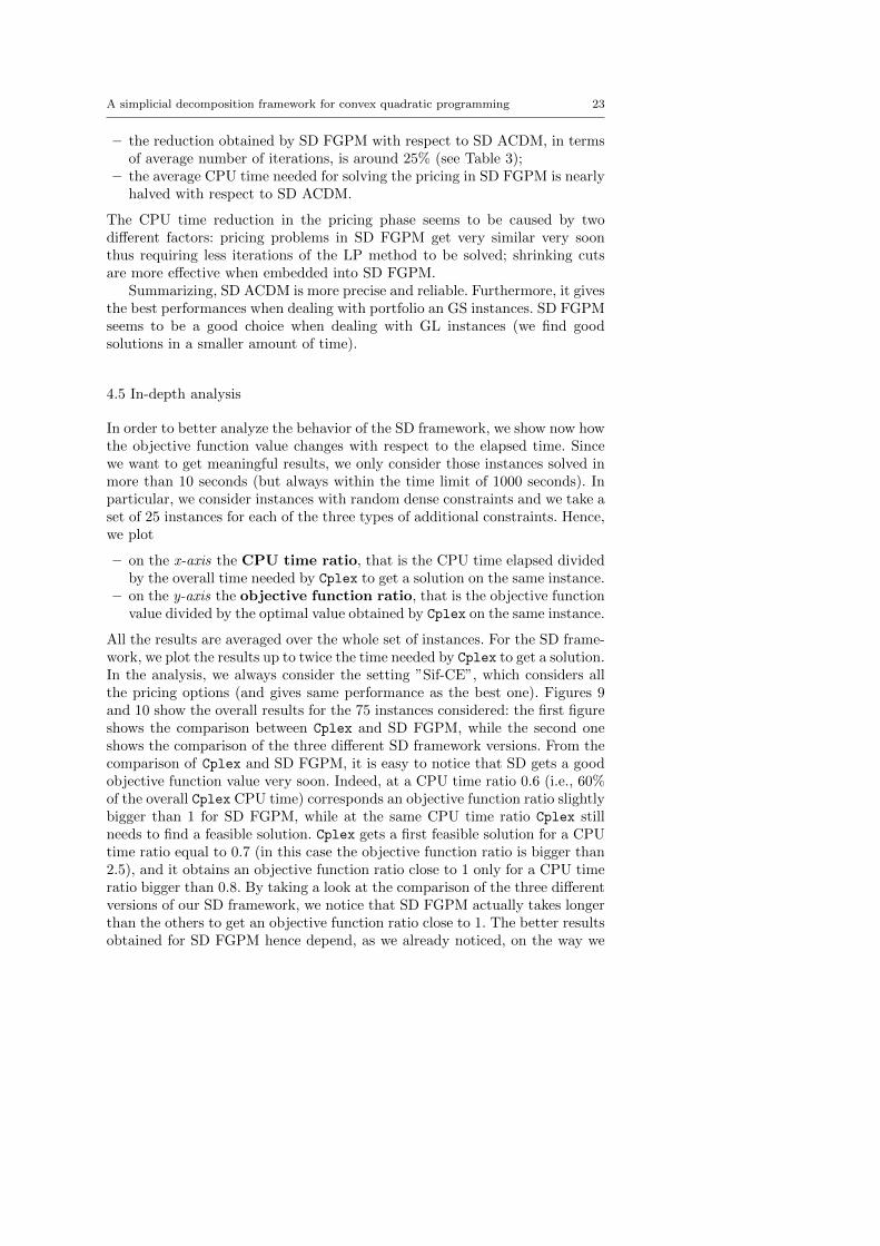
– the reduction obtained by SD FGPM with respect to SD ACDM, in termsof average number of iterations, is around 25% (see Table 3);

– the average CPU time needed for solving the pricing in SD FGPM is nearlyhalved with respect to SD ACDM.

The CPU time reduction in the pricing phase seems to be caused by twodifferent factors: pricing problems in SD FGPM get very similar very soonthus requiring less iterations of the LP method to be solved; shrinking cutsare more effective when embedded into SD FGPM.

Summarizing, SD ACDM is more precise and reliable. Furthermore, it givesthe best performances when dealing with portfolio an GS instances. SD FGPMseems to be a good choice when dealing with GL instances (we find goodsolutions in a smaller amount of time).

4.5 In-depth analysis

In order to better analyze the behavior of the SD framework, we show now howthe objective function value changes with respect to the elapsed time. Sincewe want to get meaningful results, we only consider those instances solved inmore than 10 seconds (but always within the time limit of 1000 seconds). Inparticular, we consider instances with random dense constraints and we take aset of 25 instances for each of the three types of additional constraints. Hence,we plot

– on the x-axis the CPU time ratio, that is the CPU time elapsed dividedby the overall time needed by Cplex to get a solution on the same instance.

– on the y-axis the objective function ratio, that is the objective functionvalue divided by the optimal value obtained by Cplex on the same instance.

All the results are averaged over the whole set of instances. For the SD frame-work, we plot the results up to twice the time needed by Cplex to get a solution.In the analysis, we always consider the setting ”Sif-CE”, which considers allthe pricing options (and gives same performance as the best one). Figures 9and 10 show the overall results for the 75 instances considered: the first figureshows the comparison between Cplex and SD FGPM, while the second oneshows the comparison of the three different SD framework versions. From thecomparison of Cplex and SD FGPM, it is easy to notice that SD gets a goodobjective function value very soon. Indeed, at a CPU time ratio 0.6 (i.e., 60%of the overall Cplex CPU time) corresponds an objective function ratio slightlybigger than 1 for SD FGPM, while at the same CPU time ratio Cplex stillneeds to find a feasible solution. Cplex gets a first feasible solution for a CPUtime ratio equal to 0.7 (in this case the objective function ratio is bigger than2.5), and it obtains an objective function ratio close to 1 only for a CPU timeratio bigger than 0.8. By taking a look at the comparison of the three differentversions of our SD framework, we notice that SD FGPM actually takes longerthan the others to get an objective function ratio close to 1. The better resultsobtained for SD FGPM hence depend, as we already noticed, on the way we


choose the tolerance in the master solvers. Finally, in Figure 11, we report theplots related to those instances where Cplex outperforms the SD framework.Once again, we can see that SD FGPM gets a good objective function ratiovery soon, while Cplex takes much longer to obtain a similar ratio.

SD FGPM

Cplex

0.5 1.0 1.5 2.00.0

0.5

1.0

1.5

2.0

2.5

Fig. 9 Objective function decay - Objective function ratio (y-axis) and CPU time ratio(x-axis) - SD FGPM vs Cplex.

SD Cplex

SD ACDM

SD FGPM

0.8 1.0 1.2 1.4 1.6 1.8 2.0

1.000

1.002

1.004

1.006

1.008

Fig. 10 Objective function decay - Objective function ratio (y-axis) and CPU time ratio(x-axis) - SD solvers comparison.

5 Conclusions

We presented an efficient SD framework to solve continuous convex quadraticproblems. It embeds two ad-hoc methods for solving the master problem,namely an adaptive conjugate directions based method and a fast gradientprojection method. Furthermore, three different strategies to speed up thepricing are included: an early stopping technique, a method to shrink the fea-sible region based on some specific cuts, and a sifting strategy to solve thepricing problem.


SD FGPM

Cplex

0.5 1.0 1.5 2.00

1

2

3

4

5

Fig. 11 Objective function decay - Objective function ratio (y-axis) and CPU time ratio(x-axis) - GL instances (Rb constraints).

We showed, through a wide numerical experience, that our algorithm isbetter than Cplex when dealing with instances with a dense Hessian matrixand with a number of constraints considerably smaller than the number ofvariables.

In Table 4, we summarize the recommended settings with respect to theinstances we solved. For portfolio instances (PORTFOLIO), the best mastersolver is ACDM and the best pricing option is sifting with early stopping. Forgeneric quadratic instances with a small number of constraints (SMALL m)the best master optimizer is again ACDM and the the best pricing option issifting. Finally, for generic quadratic instances with a large number of con-straints (LARGE m) the cuts play an important role (best pricing option issifting with cuts) and FGPM is the best master solver.

Master solvers Pricing options

ACDM FGPM SIFTING EARLY ST. CUTS

PORTFOLIO X × X X ×Instances SMALL m X × X × ×

LARGE m × X X × XTable 4 Best settings overview.

References

1. Beasley, J.E.: Portfolio optimization data (2016)2. Bertsekas, D.P., Scientific, A.: Convex optimization algorithms. Athena Scientific Bel-

mont (2015)3. Birgin, E.G., Martınez, J.M., Raydan, M.: Nonmonotone spectral projected gradient

methods on convex sets. SIAM Journal on Optimization 10(4), 1196–1211 (2000)4. Boyd, S., Vandenberghe, L.: Convex optimization. Cambridge university press (2004)5. Cesarone, F., Tardella, F.: Portfolio datasets (2010)


6. Condat, L.: Fast projection onto the simplex and the l1-ball. Mathematical Program-ming 158(1), 575–585 (2016)

7. Desaulniers, G., Desrosiers, J., Solomon, M.M.: Column generation, vol. 5. SpringerScience & Business Media (2006)

8. Dolan, E.D., More, J.J.: Benchmarking optimization software with performance profiles.Mathematical Programming 91(2), 201–213 (2002)

9. Gondzio, J.: Interior point methods 25 years later. European Journal of OperationalResearch 218(3), 587–601 (2012)

10. Hearn, D.W., Lawphongpanich, S., Ventura, J.A.: Restricted simplicial decomposition:Computation and extensions. Computation Mathematical Programming pp. 99–118(1987)

11. Holloway, C.A.: An extension of the frank and wolfe method of feasible directions.Mathematical Programming 6(1), 14–27 (1974)

12. IBM: Cplex (version 12.6.2) (2016). URL https://www-01.ibm.com/software/

commerce/optimization/cplex-optimizer/

13. Markowitz, H.: Portfolio selection. The Journal of Finance 7(1), 77–91 (1952)14. Michelot, C.: A finite algorithm for finding the projection of a point onto the canonical

simplex of IRn. Journal of Optimization Theory and Applications 50(1), 195–200 (1986)15. Nesterov, Y., Nemirovskii, A.: Interior-point polynomial algorithms in convex program-

ming. SIAM (1994)16. Nocedal, J., Wright, S.J.: Sequential quadratic programming. Springer (2006)17. Patriksson, M.: The traffic assignment problem: models and methods. Courier Dover

Publications (2015)18. Pshenichnyı, B.N., Danilin, I.M.: Numerical methods in extremal problems. Mir Pub-

lishers (1978)19. Ventura, J.A., Hearn, D.W.: Restricted simplicial decomposition for convex constrained

problems. Mathematical Programming 59(1), 71–85 (1993)20. Von Hohenbalken, B.: Simplicial decomposition in nonlinear programming algorithms.

Mathematical Programming 13(1), 49–68 (1977)21. WolframAlpha: Mathematica (version 10.2) (2015). URL http://www.wolfram.com/

mathematica/

22. Wright, M.: The interior-point revolution in optimization: history, recent developments,and lasting consequences. Bulletin of the American mathematical society 42(1), 39–56(2005)

23. Wright, S.J.: Primal-dual interior-point methods. SIAM (1997)24. Ye, Y.: Interior point algorithms: theory and analysis, vol. 44. John Wiley & Sons (2011)

a simplicial decomposition framework for large scale

Documents