decomposition, localization and time-averaging approaches ... · decomposition, localization and...
TRANSCRIPT

e
e
e
Faculte des Sciences Appliquees
Institut Montefiore
Departement d’Electricite, Electronique et Informatique
Decomposition, Localization and
Time-Averaging Approaches
in Large-Scale Power System
Dynamic Simulation
Liege, Belgium, July 2012
A dissertation submitted by Davide Fabozzi
in partial fulfillment of the requirements for the degree of
Doctor of Philosophy (Ph.D.) in Engineering Sciences

.

.
A mia mamma

.

The history of sparsity is an interesting example
of a development whose time was long overdue.
Why did it take so long to discover and catch on?
The answer might shed light on similar
occurrences of technological blindness.
Since the possibilities of sparsity exploitation
should have been self-evident to a village idiot,
it is perplexing how they escaped notice
by applied mathematicians. As it turned out,
sparsity was pioneered by a scattering of
problem solvers, not mathematicians.
This suggests that similar seemingly obvious
ideas may still be escaping detection,
not because of their obscurity
but because of their elusive simplicity 1
1William F. Tinney. This excerpt is taken from the 1979 issue of This Week’s Citation Classics [Tin79]: in thiscommentary, Dr. Tinney recalls the first efforts in exploiting the sparse structure of matrices, which can betraced back to 1957. Work on sparsity went unnoticed for about a decade and finally gained wider recognitiononly as late as 1968.

.

Examining Committee
Sı ch’io fui sesto tra cotanto senno 1
Prof. Christophe Geuzaine, Universite de Liege, Belgium
Prof. Jean-Louis Lilien (President of Jury), Universite de Liege, Belgium
Prof. Federico Milano, Universidad de Castilla - La Mancha, Spain
Prof. Bikash C. Pal, Imperial College London, United Kingdom
Prof. Patricia Rousseaux, Universite de Liege, Belgium
Prof. Thierry Van Cutsem (PhD advisor), Universite de Liege, Belgium
Prof. Louis Wehenkel, Universite de Liege, Belgium
Prof. Wolfram H. Wellßow, Technische Universitat Kaiserslautern, Germany
1And I was sixth amid so learn’d a band. Dante, ne Durante di Alighiero degli Alighieri, in Comedıa, laterCommedia. English translation by H. F. Cary in The Divine Comedy of Dante. In this excerpt from Canto IV ofInferno, Dante is passing through Limbo, the first circle of hell where virtuous unbaptized adults are hosted (inLatin limbus means ”edge” or ”border”). Virgil, Dante’s guide throughout this part of his journey, introduceshim to fellow poets Homer, Horace, Ovid and Lucan: they invite Dante to join their discussion, during whichDante feels his wisdom ranks sixth (i.e. last) among those great poets.
7

.

Acknowledgements
Gratia pro rebus merito debetur inemtis 1
I would like to thank my advisor, Prof. Thierry Van Cutsem, for giving me the oppor-
tunity to pursue my PhD under his guidance. The research group he leads at University of
Liege is a unique working environment, where I felt free to develop my own creativity but
at the same time I knew I could rely on his pragmatism and scientific rigor: his advice was
fundamental to direct my research towards promising areas, and to avoid dead-ends.
I wish to express my gratitude to each member of the examining committee, for devoting
their time to read this report. A special thanks to Prof. Patricia Rousseaux also for the many
enriching discussions during my PhD.
The research documented in this report has been performed, for three years, in the con-
text of the PEGASE project funded by European Commission’s Seventh Framework Pro-
gramme (grant agreement No. 211407), whose support I gratefully acknowledge.
Within this project I collaborated with the R&D department of the French transmission
system operator RTE. I would like to thank Angela S. Chieh, Patrick Panciatici and Vincent
Sermanson for welcoming me in my visits to Paris: I found extremely useful to discuss with
partners who excel in both scientific research and transmission system operator practice.
1Thanks worthily are due for things unbought. Publius Ovidius Naso (Ovid) in Amores, English translation byChristopher Marlowe.
9

The Power System Consulting group of Tractebel Engineering - GDF Suez was the co-
ordinator of the PEGASE project. I benefitted from the broad variety of skills of Tractebel
experts. Many thanks to Dr. Bertrand Haut, Karim Karoui, Dr. Christian Merckx, Christel
Moisse, Ludovic Platbrood and Fortunato Villella.
After my involvement in the PEGASE project I worked with the Canadian transmission
system operator Hydro-Quebec, TransEnergie division. Thanks to Simon Lebeau and Fran-
cis Talbot I had access to real data for my tests and this collaboration allowed me to deal
with real engineering problems.
Now that I am close to the end of my Belgian experience, I want to mention late Prof.
Paolo Marannino, thanks to whom this experience began: he encouraged me to cross the
Alps, in 2007, for the Erasmus exchange program that marked the start of my research at
University of Liege. He is deeply missed.
I owe a special thanks to Dr. Mevludin Glavic for the many insightful discussions during
our many coffee breaks outside the department entrance.
The experience in Liege was marked also by the enriching encounters of my senior PhD
colleagues, Dr. Adamantios (Diamantis) Marinakis and Dr. Ninel (Bogdan) Otomega. They
contributed to the friendly atmosphere of our research group, which I tried to pass over
to my junior PhD colleagues, Petros Aristidou and Frederic Plumier: I wish to thank them
both for our close collaboration and friendship in the last years of my PhD thesis.
Three scholars helped me finding some of the original texts for the citations I used in the
beginning of each chapter: many thanks to Prof. Laurence Bouquiaux at the Department of
Philosophy of University of Liege, Prof. Gregory Brown at the Department of Philosophy of
University of Houston, Texas, and Dr. Siegmund Probst at the Leibniz archive of Gottfried
Wilhelm Leibniz Bibliothek, Niedersachsische Landesbibliothek, Hannover, Germany.
I cannot list them all here, but I heartily thank all my friends, the old friends from Italy
as well as the people I befriended during these last 5 years in Belgium.
The last thanks go to my family, especially to my mother Giovanna, to whom this work
is dedicated, and to Elena and Max thanks to whom I will soon become an uncle.
Grazie.
10

Abstract
Il sugo di tutta la storia 1
Present-day interconnected electric power systems are the largest machines in the world.
Guaranteeing a stable supply of electric power is vital for modern societies: power systems
must be able to withstand plausible disturbances. A certain number of simulations of the
post-disturbance behavior are routinely executed by some transmission system operators to
assess that the system is operated in a secure way. Usually this assessment has to be per-
formed within a predefined time frame, using the available computing resources. Improv-
ing the simulation speed allows the operators to perform a wider assessment, thus making
better use of the available computational power. A large part of this research took place in
the context of the PEGASE project, supported by European Commission (Seventh Frame-
work Programme) and has resulted in some novel algorithms for faster dynamic simula-
tions, one of the PEGASE project main goals. First, this thesis revisits the Newton method
used to solve the differential-algebraic model. Then, three original algorithmic improve-
ments are presented, namely (i) decomposition, (ii) localization and (iii) time-averaging of
the system response. Finally, the combination of these approaches is shown to provide a fast
and reliable tool for dynamic security assessment. All the presented techniques have been
thoroughly tested on an academic system, a large real-life system and a realistic system of
unprecedented size, representative of the whole continental European synchronous grid.
1The gist (literally ”the sauce”) of the argument. Alessandro Manzoni in I Promessi Sposi (The Betrothed).
11


List of main symbols
Non si puo intendere [questo libro] se prima non s’impara
a intender la lingua, e conoscer i caratteri, ne’ quali e scritto. 1
Matrices are indicated with capital letters, vector and matrices are in bold font, vectors
are column vectors unless otherwise stated.
N number of network buses
V 2N-dimensional vector of rectangular components of bus voltages
z vector of discrete variables
x vector of continuous variables
C matrix including 0’s and 1’s linking injector currents to network equations (2N ×dim(x))
B matrix of sensitivities of injectors equations with respect to voltages (dim(x)× 2N)
A block diagonal matrix, each block being the Jacobian of injector equations with respect
to injector variables (dim(x)× dim(x))
D network matrix (2N × 2N) stemming from decomposition of bus admittance matrix
J Jacobian of both network and injectors ((2N + dim(x))× (2N + dim(x)))
1We cannot understand [this book] if we do not first learn the language and grasp the symbols, in which it iswritten. Galileo Galilei in Il Saggiatore. English translation by Thomas Salusbury in The Assayer, as quoted inThe Metaphysical Foundations of Modern Science by E. A. Burtt.
13

n number of injectors
ni number of continuous variables of injector i
zi vector of discrete variables of injector i
xi vector of continuous variables of injector i (ni)
Ci matrix including 0’s and 1’s linking injector i currents to network equations (2N× ni)
B matrix of sensitivities of injectors equations with respect to voltages (dim(x)× 2N)
Bi matrix of sensitivities of injectors equations to voltages in injector i (ni × 2N)
Ai Jacobian matrix of injector equations with respect to injector variables in injector i
(ni × ni)
CiBi Schur correction CiA−1i Bi of injector i (2N × 2N)
D Schur complement D + ∑ni=1 CiA−1
i Bi of A (2N × 2N)
Solution schemes are indicated with capital letters.
I Integrated scheme (see Chapter 3)
A Decomposed scheme using acceleration techniques (see Chapter 4)
L Localized scheme: same as A, using localization (see Chapter 5)
T Time-averaged scheme: same as I, using time-averaging (see Chapter 6)
C Combined scheme (see Chapter 7)
14
Table of Contents
1 Introduction 19
1.1 Motivation . . . . . . . . . . . . . . . . . . . . . . . . . . . . . . . . . . . . . . . 19
1.2 A classification of existing approaches . . . . . . . . . . . . . . . . . . . . . . . 20
1.3 Outline of this work . . . . . . . . . . . . . . . . . . . . . . . . . . . . . . . . . 21
1.4 Structure of the report . . . . . . . . . . . . . . . . . . . . . . . . . . . . . . . . 23
1.5 Publications . . . . . . . . . . . . . . . . . . . . . . . . . . . . . . . . . . . . . . 24
2 Power system modelling 25
2.1 Differential-algebraic models . . . . . . . . . . . . . . . . . . . . . . . . . . . . 26
2.2 Non-causal equation-based models in compact form . . . . . . . . . . . . . . 28
2.3 Non-causal equation-based hybrid models . . . . . . . . . . . . . . . . . . . . 30
2.4 Description of Nordic32 system . . . . . . . . . . . . . . . . . . . . . . . . . . . 32
2.5 Description of Hydro-Quebec system . . . . . . . . . . . . . . . . . . . . . . . 34
2.6 Description of PEGASE system . . . . . . . . . . . . . . . . . . . . . . . . . . . 37
3 Simulating power system models 41
3.1 Integration formulae . . . . . . . . . . . . . . . . . . . . . . . . . . . . . . . . . 42
3.2 Solution of nonlinear systems of equations . . . . . . . . . . . . . . . . . . . . 45
3.3 Practical application of Newton method . . . . . . . . . . . . . . . . . . . . . . 46
3.4 Step size control . . . . . . . . . . . . . . . . . . . . . . . . . . . . . . . . . . . . 48
3.5 Events and discontinuities . . . . . . . . . . . . . . . . . . . . . . . . . . . . . . 52
3.6 Dynamic time warping measure of accuracy . . . . . . . . . . . . . . . . . . . 53
15

4 Decomposing Newton iterations 57
4.1 Decomposition methods in literature . . . . . . . . . . . . . . . . . . . . . . . . 57
4.2 Bordered Block Diagonal decomposition . . . . . . . . . . . . . . . . . . . . . 60
4.3 Skipping solution of converged components . . . . . . . . . . . . . . . . . . . 66
4.4 Skipping update of Jacobian matrices . . . . . . . . . . . . . . . . . . . . . . . 68
4.5 Extension to two- and multi-port components . . . . . . . . . . . . . . . . . . 69
4.6 Scenari and results on Nordic32 system . . . . . . . . . . . . . . . . . . . . . . 71
4.6.1 Case N1 . . . . . . . . . . . . . . . . . . . . . . . . . . . . . . . . . . . . 71
4.6.2 Case N2 . . . . . . . . . . . . . . . . . . . . . . . . . . . . . . . . . . . . 72
4.6.3 Case N3 . . . . . . . . . . . . . . . . . . . . . . . . . . . . . . . . . . . . 72
4.6.4 Case N4 . . . . . . . . . . . . . . . . . . . . . . . . . . . . . . . . . . . . 75
4.6.5 Case N5 . . . . . . . . . . . . . . . . . . . . . . . . . . . . . . . . . . . . 75
4.7 Scenari and results on Hydro-Quebec system . . . . . . . . . . . . . . . . . . . 79
4.7.1 Case Q1 . . . . . . . . . . . . . . . . . . . . . . . . . . . . . . . . . . . . 79
4.7.2 Case Q2 . . . . . . . . . . . . . . . . . . . . . . . . . . . . . . . . . . . . 80
4.7.3 Case Q3 . . . . . . . . . . . . . . . . . . . . . . . . . . . . . . . . . . . . 80
4.7.4 Case Q4 . . . . . . . . . . . . . . . . . . . . . . . . . . . . . . . . . . . . 80
4.7.5 Case Q5 . . . . . . . . . . . . . . . . . . . . . . . . . . . . . . . . . . . . 85
4.7.6 Computational effort . . . . . . . . . . . . . . . . . . . . . . . . . . . . . 85
4.8 Scenari and results on PEGASE system . . . . . . . . . . . . . . . . . . . . . . 86
4.8.1 Case P1 . . . . . . . . . . . . . . . . . . . . . . . . . . . . . . . . . . . . 86
4.8.2 Case P2 . . . . . . . . . . . . . . . . . . . . . . . . . . . . . . . . . . . . 86
4.8.3 Case P3 . . . . . . . . . . . . . . . . . . . . . . . . . . . . . . . . . . . . 86
4.8.4 Computational effort . . . . . . . . . . . . . . . . . . . . . . . . . . . . . 89
4.9 Chapter conclusion . . . . . . . . . . . . . . . . . . . . . . . . . . . . . . . . . . 91
5 Relaxing accuracy in space 95
5.1 Spatial accuracy relaxation in literature . . . . . . . . . . . . . . . . . . . . . . 95
5.2 Localization in the decomposed Newton scheme . . . . . . . . . . . . . . . . . 97
5.3 Latency detection algorithm . . . . . . . . . . . . . . . . . . . . . . . . . . . . . 99
5.4 Localization results on Nordic32 system . . . . . . . . . . . . . . . . . . . . . . 102
5.4.1 Case N1 . . . . . . . . . . . . . . . . . . . . . . . . . . . . . . . . . . . . 102
5.4.2 Case N2 . . . . . . . . . . . . . . . . . . . . . . . . . . . . . . . . . . . . 103
16

5.4.3 Other cases . . . . . . . . . . . . . . . . . . . . . . . . . . . . . . . . . . 103
5.5 Localization results on Hydro-Quebec system . . . . . . . . . . . . . . . . . . 108
5.5.1 Case Q2 . . . . . . . . . . . . . . . . . . . . . . . . . . . . . . . . . . . . 108
5.5.2 Case Q4 . . . . . . . . . . . . . . . . . . . . . . . . . . . . . . . . . . . . 108
5.5.3 Computational effort . . . . . . . . . . . . . . . . . . . . . . . . . . . . . 108
5.5.4 Other cases . . . . . . . . . . . . . . . . . . . . . . . . . . . . . . . . . . 110
5.6 Localization results on PEGASE system . . . . . . . . . . . . . . . . . . . . . . 110
5.6.1 Cases P1, P2 and P3 . . . . . . . . . . . . . . . . . . . . . . . . . . . . . 110
5.6.2 Computational effort . . . . . . . . . . . . . . . . . . . . . . . . . . . . . 116
5.7 Chapter conclusion . . . . . . . . . . . . . . . . . . . . . . . . . . . . . . . . . . 119
6 Relaxing accuracy in time 121
6.1 Temporal accuracy relaxation in literature . . . . . . . . . . . . . . . . . . . . . 121
6.2 Time-averaging of continuous dynamics . . . . . . . . . . . . . . . . . . . . . . 123
6.3 Handling of discrete dynamics . . . . . . . . . . . . . . . . . . . . . . . . . . . 125
6.4 Step size and step size reduction . . . . . . . . . . . . . . . . . . . . . . . . . . 128
6.5 Example of cycling between flows . . . . . . . . . . . . . . . . . . . . . . . . . 131
6.6 Time-averaging results on Nordic32 system . . . . . . . . . . . . . . . . . . . . 133
6.6.1 Case N1 . . . . . . . . . . . . . . . . . . . . . . . . . . . . . . . . . . . . 133
6.6.2 Case N2 . . . . . . . . . . . . . . . . . . . . . . . . . . . . . . . . . . . . 135
6.6.3 Case N3 . . . . . . . . . . . . . . . . . . . . . . . . . . . . . . . . . . . . 135
6.6.4 Case N4 . . . . . . . . . . . . . . . . . . . . . . . . . . . . . . . . . . . . 135
6.7 Time-averaging results on Hydro-Quebec system . . . . . . . . . . . . . . . . 139
6.7.1 Case Q2 . . . . . . . . . . . . . . . . . . . . . . . . . . . . . . . . . . . . 139
6.7.2 Case Q3 . . . . . . . . . . . . . . . . . . . . . . . . . . . . . . . . . . . . 139
6.7.3 Case Q4 . . . . . . . . . . . . . . . . . . . . . . . . . . . . . . . . . . . . 139
6.7.4 Computational effort . . . . . . . . . . . . . . . . . . . . . . . . . . . . . 142
6.8 Time-averaging results on PEGASE system . . . . . . . . . . . . . . . . . . . . 142
6.8.1 Cases P1 and P2 . . . . . . . . . . . . . . . . . . . . . . . . . . . . . . . 142
6.8.2 Computational effort . . . . . . . . . . . . . . . . . . . . . . . . . . . . . 144
6.9 Chapter conclusion . . . . . . . . . . . . . . . . . . . . . . . . . . . . . . . . . . 145
17

7 Combining detailed simulation with accuracy relaxation techniques 147
7.1 How accurate is a detailed simulation? . . . . . . . . . . . . . . . . . . . . . . . 148
7.2 Combination of short- and long-term simulations . . . . . . . . . . . . . . . . 149
7.3 Combining detailed and relaxed accuracy simulations . . . . . . . . . . . . . 151
7.4 Combined simulation results on Nordic32 system . . . . . . . . . . . . . . . . 153
7.4.1 Case N1 . . . . . . . . . . . . . . . . . . . . . . . . . . . . . . . . . . . . 154
7.4.2 Case N2 . . . . . . . . . . . . . . . . . . . . . . . . . . . . . . . . . . . . 154
7.4.3 Case N3 . . . . . . . . . . . . . . . . . . . . . . . . . . . . . . . . . . . . 154
7.4.4 Case N5 . . . . . . . . . . . . . . . . . . . . . . . . . . . . . . . . . . . . 158
7.5 Combined simulation results on Hydro-Quebec system . . . . . . . . . . . . . 159
7.5.1 Case Q1 . . . . . . . . . . . . . . . . . . . . . . . . . . . . . . . . . . . . 160
7.5.2 Case Q2 . . . . . . . . . . . . . . . . . . . . . . . . . . . . . . . . . . . . 160
7.5.3 Case Q3 . . . . . . . . . . . . . . . . . . . . . . . . . . . . . . . . . . . . 160
7.5.4 Case Q4 . . . . . . . . . . . . . . . . . . . . . . . . . . . . . . . . . . . . 160
7.5.5 Case Q5 . . . . . . . . . . . . . . . . . . . . . . . . . . . . . . . . . . . . 160
7.5.6 Computational effort . . . . . . . . . . . . . . . . . . . . . . . . . . . . . 164
7.6 Combined simulation results on PEGASE system . . . . . . . . . . . . . . . . 164
7.6.1 Cases P1, P2 and P3 . . . . . . . . . . . . . . . . . . . . . . . . . . . . . 164
7.6.2 Computational effort . . . . . . . . . . . . . . . . . . . . . . . . . . . . . 167
7.7 Chapter conclusion . . . . . . . . . . . . . . . . . . . . . . . . . . . . . . . . . . 167
8 General conclusion 173
8.1 Summary of work and main contributions . . . . . . . . . . . . . . . . . . . . 173
8.2 Directions for future work . . . . . . . . . . . . . . . . . . . . . . . . . . . . . . 175
Appendices 177
A.1 Explicit reference frame . . . . . . . . . . . . . . . . . . . . . . . . . . . . . . . 177
A.2 Synchronous machine model . . . . . . . . . . . . . . . . . . . . . . . . . . . . 183
A.3 Restorative load model . . . . . . . . . . . . . . . . . . . . . . . . . . . . . . . . 187
A.4 Computation of BDF coefficients . . . . . . . . . . . . . . . . . . . . . . . . . . 191
A.5 Implementation aspects . . . . . . . . . . . . . . . . . . . . . . . . . . . . . . . 193
Bibliography 195
18
Chapter1
Introduction
Li arcieri prudenti pongono la mira
assai piu alta che il loco destinato 1
1.1 Motivation
Dynamic simulations under the phasor approximation are routinely used throughout the
world for the purpose of checking the response of electric power systems to large distur-
bances. Over the last decades, dynamic models have been standardized and simulation
tools have been developed to meet the specifics of power system models [Kun94].
However, in spite of the increase in computational power, dynamic simulations of large-
scale systems remain time consuming. Indeed, they require solving a large set of nonlinear
stiff hybrid Differential-Algebraic Equations (DAEs). A large interconnected system may
involve hundreds of thousands of such equations spanning very different time scales and
undergoing many discrete transitions imposed by limiters, switching devices, etc.
There are applications where this computational effort is an obstacle. Let us quote non
exhaustively: (i) detailed operator training simulator; (ii) analysis of large set of scenari, for
instance in Monte-Carlo simulations; (iii) Dynamic Security Assessment (DSA), particularly
in real-time applications.1The clever archers take aim much higher than the mark. Niccolo di Bernardo dei Machiavelli, in Il Principe,
English translation by W. K. Marriott in The Prince.
19

The last item is probably the most constraining [gC07]. This is even more true when,
instead of the 10 to 20 seconds simulated for short-term stability, the evolution is computed
until a new steady state is reached, which requires simulating long-term dynamics over
several minutes after the initiating event. This computational burden justifies the fact that
many control centers routinely perform static security assessment, typically AC (if not DC
for some problems) power flows and resort infrequently to DSA. Static computations seek
the post-contingency equilibrium point, without considering the system evolution that may
- or may not - lead to that point.
One can expect, however, that the need for DSA will go increasing. Operation of non-
expandable grids closer to their stability limits and unplanned generation patterns owing
to the penetration of renewable energy sources require dynamic studies. Furthermore, un-
der the pressure of electricity markets and with the support of active demand response,
it is likely that system security will be more and more guaranteed by emergency controls
responding to the disturbance. In this context, security analysis requires checking the se-
quence of events that take place after the initiating disturbance, a task for which static
calculation of the operating point in a guessed final configuration is inappropriate. Last, in
stressed conditions, power flow computations may diverge, thus leaving operators with no
information in circumstances where the support of computer simulation is mostly needed.
1.2 A classification of existing approaches
Several approaches have been tried over the past decades to speed-up time simulation. They
can be roughly classified into relaxation and direct methods [PCLG+11].
Approaches by relaxation rely on a decomposition of the set of equations in sub-domains
in which the equations are solved independently. Information, such as states or time evo-
lution at the boundaries, is then exchanged between sub-domains before a new iteration
is carried out [MR06]. The advantage of these methods lies in the ability to solve the sub-
domains in parallel using multiple processors/cores [CZBT91] or even graphics processing
units [JMD10], while the main drawback is the convergence degradation due to the above
mentioned iterations. Examples of relaxation methods that have been applied to power
systems are: waveform relaxation on a time interval [ISCP87] or at one time step [JMD09],
multi-rate simulation [CC94], and Picard iterations [LSBTC90].
Among the direct methods, the Newton method is prominent. It is used to solve the
20
nonlinear equations stemming from the algebraic equations of the model and from the
algebraization of the differential equations at a given time step. A major advantage of
this method lies in its convergence properties. In its standard form, it requires solving
a large system of linear equations based on a sparse Jacobian matrix [KMC08]. For power
system dynamic models, a salient feature of this matrix is its Bordered Block Diagonal (BBD)
structure. It allows solving the linear equations in a decomposed way, the numerous small
diagonal blocks and their Schur complement [Zha05] being processed separately. This also
opens the way for some parallel processing, while retaining the good convergence property
of the direct Newton method. The BBD structure is exploited in VLSI circuit simulation
for instance [Ogr94], and its application to power system dynamics can be traced back
to [Boe77]. Since then, the technique has been used in some production grade simulation
packages (e.g. [Kun94] p. 863) although, to the author’s knowledge, there are few references
on the subject.
1.3 Outline of this work
In this work the BBD structure is exploited in a novel way that is still suitable to some
parallel processing [HBJVN77], although it is not the topic of this thesis. The proposed
algorithm resorts to the above mentioned decomposition: (i) to solve only the parts of
the system that need to be solved, and (ii) to avoid global updates of the Jacobian when
local updates would suffice. Both situations occur very often in large-scale power system
simulation.
The above cited methods speed up the Newton method while retaining full accuracy. An
additional possibility consists in speeding-up numerical simulations by relaxing accuracy
to an extent compatible with DSA needs. Two tracks were followed in this work, leading to
relaxation of accuracy in space and in time, respectively.
Previous attempts to speed up dynamic simulation often relied on model reduction or
model simplification. Models are simplified in order to become smaller and/or less stiff.
An example that combines reduction in size and stiffness is the quasi steady-state approx-
imation of long-term dynamics [VCV08]. It consists in replacing the short-term dynamics
by their equilibrium equations while the simulation focuses on the long-term dynamics.
However, automatic methods to simplify real-life, hybrid power system models are yet to
be developed. Hence, the current practice consists in either creating and maintaining a
21

reduced model for a specific system, or adopting right away a generic simplified model.
The concept of accuracy relaxation considered in thesis is definitely different from model
simplification, in so far as the same model as in detailed simulations is adopted. Thus, no
effort is spent in model reduction; instead the gain in efficiency comes from the relaxable
accuracy solver that is used.
Spatial relaxation of accuracy exploits the fact that, in a large-scale system, most of dis-
turbances give rise to localized effects, i.e. some system components do not participate
much in the dynamic response. This holds true at least for some periods of time and is
more noticeable in long-term simulations. Localization concepts have been used in time-
domain simulation in the variable partitioning multi-rate method [CC08]. Adaptations of
this concept have been applied also to static security analysis [Bra93], mainly in extensions
of the sparse vector method [TBC85] known as zero mismatch approach [BT89], approxi-
mate sparse vector method [BET91] and adaptive localization [EPT92].
Similar techniques have been used successfully in the simulation of VLSI circuits [HSV81].
In VLSI simulation, the system components which are nearly unaffected by a disturbance
are called latent, and the objective is to skip useless numerical operations relative to a hope-
fully large proportion of latent blocks. To this purpose, the network is torn into one main
circuit and many other blocks in order to obtain a block-bordered diagonal structure favor-
able to latency exploitation. The already converged sub-networks are not solved.
With temporal relaxation of accuracy we refer to the fact that some fast components
of the response may not be of interest, especially in long-term simulations. In nonlinear
dynamical systems theory, the procedure of replacing a vector field by its average (over
time or an angular variable) in order to obtain asymptotic approximations to the original
system is called averaging [SVM07]. A less rigorous but straightforward way to obtain
averaged responses is by using a step size which is large with respect to the neglected
dynamics. Once more, no simplification is performed on the models, i.e. they are the same
as in detailed simulation. Significant reductions of the computational effort can be expected
from such large steps.
It is known that an L-stable method must be used to integrate with steps significantly
larger than the smallest system time constants [AP98, CK06]. For larger and larger step
sizes, the trajectory converges towards a solution that satisfies the equilibrium equations
of the neglected dynamics. Those methods have been used to simulate quasi-sinusoidal
power system models [FVC09, WC11] as well as other engineering problems (e.g. [BW98]).
22

Among them, the Backward Euler method was proposed to suppress numerical oscillations
in electromagnetic transient simulations [ML89]. On the other hand, the price to pay with
L-stable methods is that they overdamp oscillations whose period is comparable to the step
size [AP98].
For a large class of continuous-time dynamics, in so far as accuracy can be somewhat re-
laxed, the step size of an L-stable method is limited only by the convergence of the Newton
iterations used to solve the algebraized equations [FVC09]. However, power system mod-
els are also hybrid and the proper handling of discrete events requires some caution when
the time step is increased. To the author’s knowledge, this aspect has been relatively less
investigated in the literature; our preliminary investigations were reported in [FCPVC11].
When a power system is subject to a large disturbance (typically a fault), its dynamic
response can be decomposed into a short-term and a long-term period, the former requiring
a more accurate solution than the latter [KOO+93].
In order to speed up dynamic simulation, with our main focus being on the long-term,
we advocate the use of a combination of detailed dynamic simulation in the short-term
with relaxation of accuracy in the long-term by means of localization and time-averaging.
The advantage of the proposed method lies in the seamless integration between detailed
short-term simulation and relaxed-accuracy long-term simulation.
1.4 Structure of the report
This report is organized as follows. In Chapter 2, power system modelling is revisited,
along with the description of the three test systems used throughout this thesis. Chapter
3 is devoted to solution methods. Chapter 4 focuses on speeding up the Newton scheme
by infrequently updating Jacobian sub-matrices and skipping iterations on converged com-
ponents, without degradation of accuracy. Chapters 5 and 6 deal with the relaxation of
accuracy in space and in time, respectively, in order to obtain faster simulations. In Chap-
ter 7, novel ways of combining accurate simulation with localization and time-averaging
are discussed. Also, this final chapter provides the author’s recommendations on how to
achieve faster dynamic simulations by accepting a fair compromise between efficiency and
accuracy. Simulation results obtained with the application of each proposed technique are
presented in the corresponding chapter.
Appendices close this thesis. They deal with the choice of angle and speed references
23

in A.1, the adopted synchronous machine and load models (A.2 and A.3, respectively),
the computation of the coefficients of the numerical integration method (A.4) and technical
information on how the simulation results were obtained (A.5).
1.5 Publications
This thesis expands material which has been published, or is under revision, in journals
and conferences:
[FCHVC12] D. Fabozzi, A. S. Chieh, B. Haut, and T. Van Cutsem. Fast dynamic sim-
ulations of large power systems. Part I: Accelerated and localized Newton
scheme and Part II: Combined detailed-simplified simulation. Submitted and
now under revision for publication in IEEE Trans. Power Syst., 2012.
[FVC11a] D. Fabozzi and T. Van Cutsem. Assessing the proximity of time evolutions
through dynamic time warping. IET Generation, Transmission & Distribution,
5(12):1268–1276,Dec. 2011.
[FCPVC11] D. Fabozzi, A. S. Chieh, P. Panciatici, and T. Van Cutsem. On simplified
handling of state events in time-domain simulation. In Proc. 17th Power
System Computation Conference (PSCC), pages 1–9, Aug. 2011.
[FVC11b] D. Fabozzi and T. Van Cutsem. On angle references in long-term time-
domain simulations. IEEE Trans. Power Syst., 26(1):483–484, Feb. 2011.
[FVC10] D. Fabozzi and T. Van Cutsem. Localization and latency concepts applied
to time simulation of large power systems. In Proc. 2010 Bulk Power System
Dynamics and Control - VIII IREP Symposium, pages 1–14, Aug. 2010.
[FVC09] D. Fabozzi and T. Van Cutsem. Simplified time-domain simulation of de-
tailed long-term dynamic models. In Proc. 2009 IEEE PES General Meeting,
pages 1–8, July 2009.
24

Chapter2
Power system modelling
Il semble que la perfection soit atteinte
non quand il n’y a plus rien a ajouter,
mais quand il n’y a plus rien a retrancher 1
In this chapter, the models used for short and long term stability calculations are de-
scribed. Some standard models of both the network and the dynamical parts of the system,
together with the choice of reference axes are analysed and revisited. It will be discussed
how the chosen non-causal equation-based hybrid modelling can encompass the standard
model used in stability studies, but provides more flexibility with respect to the latter, es-
pecially regarding the modelling of the algebraic and discrete parts.
Examples are given on two academic cases, that despite their simplicity are representa-
tive of the modelling issues that can be met in more complex, realistic power system models,
such as the synchronous machine and restorative load models reported in Appendix A.2
and A.3, respectively. The description of the test systems used throughout this thesis closes
this chapter: the three test systems chosen offer a wide variety since they include a small
academic system (Nordic32), one large real system (Hydro-Quebec), and one very large
realistic system (PEGASE).
1A designer knows he has achieved perfection not when there is nothing left to add, but when there is nothing left totake away. Antoine de Saint-Exupery, in Terre des Hommes, English translation by L. Galantiere in Wind, Sand andStars.
25

2.1 Differential-algebraic models
The Differential-Algebraic (DA) models of a power system used in stability studies can be
written as:
0 = D V− I (2.1)
0 = ψn(y, w, z, V, I, ωre f ) (2.2)
0 = ψc(y, w, z, V, I, ωre f ) (2.3)
w = ψd(y, w, z, V, I, ωre f ) (2.4)
z(t+j ) = ψz(y, w, z(t−j ), V, I, ωre f ) (2.5)
The equations above make up a system of stiff and hybrid differential-algebraic equations.
The definition of stiffness is controversial, as it relates both to the numerical difficulties
encountered in the solution of a stiff systems with some specific solvers and to the coexis-
tence of fast and slow components in system dynamics [AP98, CK06]. Further discussion
on the former definition can be found in Chapter 3, while Chapters 6 and 7 are devoted to
the latter.
Under the quasi-sinusoidal approximation, all current and voltage phasors are projected
onto orthogonal reference axes, denoted by x and y respectively, rotating at the angular
speed ωre f (the choice of the latter is discussed later in this section). Thus the vector of
complex currents is decomposed into its ix and iy components, and the vector of complex
bus voltages similarly into vx and vy. The network equations take on the form:
ix + jiy = (G + jB)(vx + jvy) (2.6)
where G and B are respectively the conductance and susceptance matrices, i.e. the real and
imaginary parts of the bus admittance matrix. Decomposing and re-assembling (2.6) yields: G −B
B G
vx
vy
− ix
iy
= 0 (2.7)
By reordering the voltage components with the Vxi variable relative to bus i occupying the
position 2i− 1 and Vyi the position 2i, and similarly for the current components, (2.7) can
be rewritten as in (2.1), where D is a sparse, structurally symmetric matrix and V (resp. I)
collects all voltage (resp. current) components.
Equation (2.2) connects the network to the various components: for instance, in case of
a synchronous machine, those are the stator equations. Other algebraic equations, coming
26

for instance from controllers or physical laws, are included in (2.3). Vector y is made up of
the corresponding algebraic variables.
Vector w groups the differential variables of all devices whose dynamics are described
by (2.4), a set of Ordinary Differential Equations (ODEs).
Note that the DA model of a power system is often written in more compact form (e.g.
[Kun94]). Assuming that (2.2) and (2.3) can be transformed to express y and I as functions
of the other variables, those expressions are substituted in (2.1) and (2.4) to obtain a DA
model that has only V as algebraic states:
0 = ma(w, V) (2.8)
w = md(w, z, V) (2.9)
z(t+j ) = mz(w, z(t−j ), V) (2.10)
This transformation of (2.2) and (2.3), however, may be impractical, if not impossible for
some models, e.g. the synchronous machine model which includes saturation effects. The
above mentioned elimination of y and I is a typical step of input-output oriented modelling,
also referred to as causal in the dynamic simulation literature [CK06] as opposed to non-
causal models. The advantages of non-causal modelling are further discussed in Section
2.2.
Finally, equation (2.5) takes into account the discrete dynamics of the system such as re-
sponses of discrete controls or changes of flows in continuous-time equations, an important
feature of power system dynamic simulation [HP00]. The respective discrete variables are
stored in z.
Continuous-time states w evolve over intervals of time. The algebraic variables in V, I
and y can also vary over instants, when some z components change. The discrete states
z evolve over instants. With the notation of (2.5), z changes from z(t−k ) to z(t+k ) at time
instants tk dictated by events, as it will be explained in detail in Section 2.3.
The choice of the speed ωre f at which the xy reference axes rotate is arbitrary and can
be made for convenience. Standard practices are either to choose the nominal angular
frequency ωre f = 2π fo, where fo is the nominal system frequency, either to adopt the
Center-Of-Inertia (COI) reference frame initially proposed in [TS72]. A recent contribution
[Mil12] reports on extraneous instabilities which can possibly arise in systems with non-
synchronous distributed energy resources due to the reference frame used. For different
reasons, that will be analyzed in detail in Appendix A.1, we preferred resorting to the
27
“explicit” COI reference approach that we proposed in [FVC11b]. This approach consists
of using, in Eqs. (2.2-2.5), at each instant the value of ωre f at the previous time step, which
can be computed explicitly; this allows eliminating ωre f from the set of variables.
2.2 Non-causal equation-based models in compact form
In the previous section we introduced the difference between causal and non-causal models
equations. An equation is causal [CK06] when the equal sign is interpreted as an assignment
more than an equality: this is typical of block-diagram modelling. While on one hand block-
diagram modelling represents a major advance by allowing a graphical representation of a
model, on the other hand, it forces to assign the output as a function of the input [Lar04].
Moreover, the interconnection of different subsystems may require to change the model
description whenever this brings a change in causality.
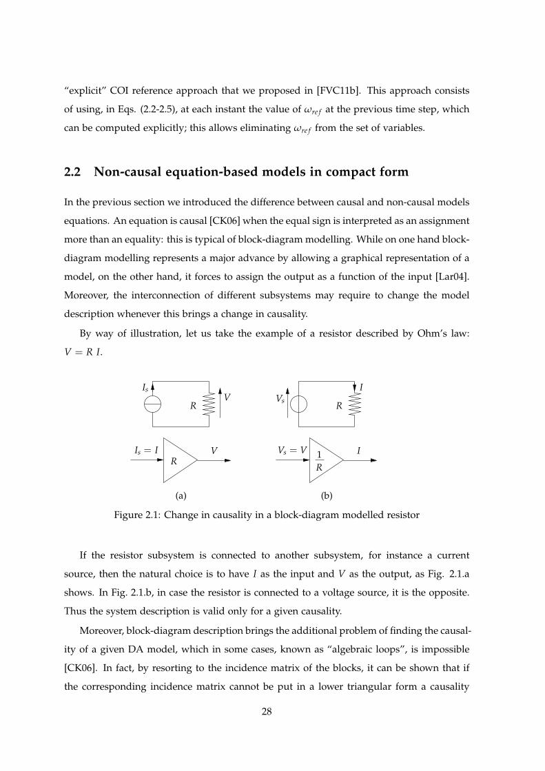
By way of illustration, let us take the example of a resistor described by Ohm’s law:
V = R I.
V I
R1
R
(a) (b)
R R
Is IV Vs
Vs = VIs = I
Figure 2.1: Change in causality in a block-diagram modelled resistor
If the resistor subsystem is connected to another subsystem, for instance a current
source, then the natural choice is to have I as the input and V as the output, as Fig. 2.1.a
shows. In Fig. 2.1.b, in case the resistor is connected to a voltage source, it is the opposite.
Thus the system description is valid only for a given causality.
Moreover, block-diagram description brings the additional problem of finding the causal-
ity of a given DA model, which in some cases, known as “algebraic loops”, is impossible
[CK06]. In fact, by resorting to the incidence matrix of the blocks, it can be shown that if
the corresponding incidence matrix cannot be put in a lower triangular form a causality
28

cannot be established. A relevant example is shown in Appendix A.2 with the description
of the adopted synchronous machine model including saturation, which indeed includes
an algebraic loop.
An equation is non-causal when it expresses a relation between peers more than a hi-
erarchy of signals: this is typical of physical modelling. The physical modelling approach
expresses constraints on variables which have to be obeyed regardless of any causality: this
approach naturally leads to equation-based models which can then easily be interconnected
in order to form more complex systems [PC11].
The advantages of equation-based over block diagram modelling will be further dis-
cussed in Section 2.3 in the context of hybrid systems and in Appendix A.2 with the afore-
mentioned algebraic loop problem.
Without loss of generality, the model of Eqs. (2.1-2.5) can be rewritten in a non-causal
equation-based compact form as:
0 = D V− C x = g(x, V) (2.11)
Γ(z) x = φ(x, z, V) (2.12)
z(t+j ) = h(x, z(t−j ), V) (2.13)
in which the expanded state vector x contains the current components ix and iy, the alge-
braic variables y and the differential states w. Equation (2.11) is essentially the same as (2.1)
and will be used either in matrix form or in g function form, for writing convenience. C
is a matrix with zero’s and one’s whose purpose is to extract the current components from
x. Equation (2.12) encompasses both the algebraic equations (2.2, 2.3) and the differential
equations (2.4). Γ is a diagonal matrix with (Γ)`` = 0 if the `-th equation (2.12) is algebraic,
and (Γ)`` = 1 if the `-th equation (2.12) is differential. Equation (2.13) is unchanged with
respect to (2.5). The dependence of Γ(z) with z is clarified in the next section.
The continuous-time dynamics equations (2.11-2.12) deal with the network and various
phenomena and controls, ranging from the short-term dynamics of power plants, static var
compensators, induction motors, etc., to the long-term dynamics of secondary frequency
control, load self restoration, etc. These equations can be either algebraic or differential.
Vector x includes the corresponding (differential and algebraic) state variables, such as
rectangular components of bus voltages, rotor angles, flux linkages, motor slips, controller
state variables, etc. The components of x take values in R or in an interval of R.
29

2.3 Non-causal equation-based hybrid models
Power systems are also hybrid systems, i.e. they involve variables which change at specific
instants of time [HP00].
The discrete-time equations (2.13) capture:
1. the response of discrete controls and protections acting with various delays in auto-
matic shunt compensation, secondary frequency and voltage control, load tap chang-
ers, phase shifting transformers, overexcitation limiters, etc. The corresponding com-
ponents of z are shunt susceptances, generator setpoints, transformer ratios, etc.
2. the change in continuous-time equations caused by limits, switches, minimum gates,
hysteresis, etc. The corresponding variables z act as “switches”. Note that the diago-
nal entries of Γ may vary with z, as suggested by (2.12), since a change in z may cause
an equation to change from differential to algebraic and vice versa.
The components of z take values in a countable subset of R.
A classical example of the second category above is the integrator with non-windup
limit, shown in Fig. 2.2.a.
z = 1z = 0
x ≥ 0
x = xmax
x < 0
x = xmax x = u
u x
xmax
s
1
(b)(a)
Figure 2.2: Integrator with non-windup limit
Let us define z as a discrete variable with value 1 if x < xmax and value 0 if x = xmax.
This system is described by the following continuous-time equation of type (2.12):
z x = z u + (1− z) (x− xmax)
30
Thus, Γ(z) = z. The changes in z can be described by the state transition diagram of Fig. 2.2.b
[Lyg04, CK06].
Continuous-time states x evolve over intervals of time. The algebraic states in x and V
can also vary over instants, when some z components change. The discrete states z evolve
over discrete instants. With the notation of Eq. (2.13), z changes from z(t−k ) to z(t+k ) at time
instants tk dictated by events. In the example of Fig. 2.2, the events are the transitions from
z = 0 to z = 1 and vice versa.
The dynamic behavior over a continuous interval according to Eqs. (2.11-2.12) is referred
to as flow. The variation of some components of z according to Eq. (2.13) causes the passage
from one flow to another at one point in time. This passage is referred to as a jump.
Events are classified according to whether it is possible or not to forecast when they
take place [CK06]. In the former case, they are called time events, and in the latter case,
state events. State events take place when a jump condition is satisfied, as a result of system
evolution. It is usually possible to specify the event condition as a zero-crossing function,
i.e. the event takes place when the value of that function passes through zero. A general
solver is thus in charge of monitoring the zero-crossing functions in order to identify the
event times, as will be detailed in Section 3.5.
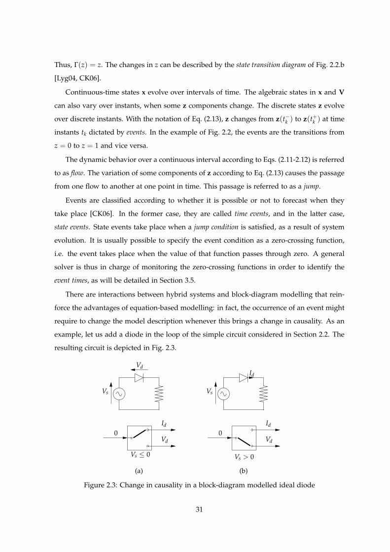
There are interactions between hybrid systems and block-diagram modelling that rein-
force the advantages of equation-based modelling: in fact, the occurrence of an event might
require to change the model description whenever this brings a change in causality. As an
example, let us add a diode in the loop of the simple circuit considered in Section 2.2. The
resulting circuit is depicted in Fig. 2.3.
0Id
Vd
Vs > 0
(b)
0Id
Vd
Vs ≤ 0
(a)
Vs
Id
Vs
Vd
Figure 2.3: Change in causality in a block-diagram modelled ideal diode
31

When the diode is blocking, i.e. Vd and Vs are non positive, the diode equation is Id = 0,
as Fig. 2.3.a shows. Otherwise, as shown in Fig. 2.3.b, when the diode is conducting,
its equation is Vd = 0. This implies a change in causality for the diode but also for the
resistor: in fact, in the former case, the resistor current is given (I = Id = 0) and the
voltage is computed as in Fig. 2.1.a, while in the latter case the resistor voltage is given
(V = Vs−Vd = Vs) and the current is computed from the block diagram shown in Fig. 2.1.b.
The hybrid system example above, together with its continuous part considered in Sec-
tion 2.2, shows that it is very likely that changes in causality happen when dealing with
connections of even very simple systems, both continuous and hybrid. This consideration,
together with the algebraic loop problem mentioned in Section 2.2 which is likely to be
present in realistic power system models (as shown in Appendix A.2), motivates the use
of non-causal equation-based hybrid modelling. Another example of this model is given in
Appendix A.3 with the description of the restorative load model adopted in our simulations.
2.4 Description of Nordic32 system
The proposed system is a variant of the so-called Nordic32 test system, proposed by K.
Walve1 and detailed in [Stu95]. As indicated in this reference, the system is fictitious but
similar to the Swedish and Nordic system (at the time of setting up this test system). The
system includes 52 (generator and transmission) buses and 80 branches. When including
the distribution buses and transformers, there are a total of 74 buses and 102 branches, re-
spectively. Appendices A.2 and A.3 describe the synchronous machine and the load model,
respectively. The synchronous machines are equipped with generic excitation systems, volt-
age regulator, power system stabilizers, speed governors and turbine models.
The one-line diagram is shown in Fig. 2.4. This system consists of four areas:
• “North” with hydro generation and some load
• “Central” with much load and thermal power generation
• “Equiv” connected to the “North”, it includes a very simple equivalent of an external
system
• “South” with thermal generation, rather loosely connected to the rest of the system.
1at that time with Svenska Kraftnat, the Swedish transmission system operator.
32

g20
g16
g17
g18
g2g9
g1 g3g10
g5
g4
g12
g8
g13
g14
g7
g6
g15
g11
g19
4011
4012
1011
1012 1014
1013
10221021
2031
cs
404640434044
40324031
4022 4021
4071
4072
4041
1042
10451041
4063
40611043
1044
4047
4051
40454062
400 kV
220 kV
130 kV synchronous condenserCS
NORTH
CENTRAL
EQUIV.
SOUTH
4042
2032
Figure 2.4: The Nordic32 system
33

The system has rather long transmission lines of 400-kV nominal voltage. Figure 2.4
shows the structure of the 400-kV backbone, along with the representation of some regional
system operating at 220 and 130 kV.
The nominal frequency is 50 Hz. Frequency is controlled through the speed governors
of the hydro generators in the North and Equiv areas only. g20 is an equivalent generator,
with a large participation in primary frequency control. The thermal units of the Central
and South areas do not participate in this control.
The system is heavily loaded with large transfers essentially from North to Central areas.
Secure system operation is limited by transient (angle) and long-term voltage instability.
The contingencies likely to yield voltage instability are:
• the tripping of a line in the North-Central corridor, forcing the North-Central power
to flow over the remaining lines;
• the outage of a generator located in the Central region, compensated (through speed
governors) by the Northern hydro generators, thereby causing an additional power
transfer over the North-Central corridor.
The maximum power that can be delivered to the Central loads is strongly influenced
by the reactive power capabilities of the Central and some of the Northern generators. Their
reactive power limits are enforced by OverExcitation Limiters (OELs). On the other hand,
Load Tap Changers (LTCs) aim at restoring distribution voltages and hence load powers.
If, after a disturbance (such as a generator or a line outage), the maximum power that can
be delivered by the combined generation and transmission system is smaller than what the
LTCs attempt to restore, voltage instability results. The latter is of the long-term type. It is
driven by OELs and LTCs and takes place in one to two minutes after the initiating event.
A similar mechanism takes place in case of a demand increase.
The Nordic32 system is used to provide examples of the dynamic phenomena of interest,
but its computational effort measures will not be given because they are not significant due
to the small size of the system.
2.5 Description of Hydro-Quebec system
Hydro-Quebec is the transmission system operator of the Quebec province, Canada. The
Hydro-Quebec system model used has been provided to us by the TransEnergie division
34

in order to investigate the performance of the proposed solver on a real-life system, which
due to its characteristics requires extensive use of dynamic simulation.
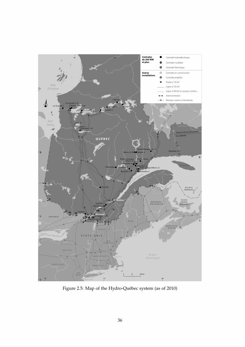
A system map is shown in Fig. 2.5.
The model includes 2204 buses and 2919 branches, whose nominal voltage ranges from 6
to 735 kV. 135 synchronous machines are represented in detail together with their excitation
systems, voltage regulators, power system stabilizers, speed governors and turbines. 976
restorative loads of the type described in Appendix A.3 are also present. The resulting
system has 11774 differential-algebraic equations and 2695 discrete variables. The peak
load is 35 000 MW.
Reference [TBS99] provides a brief overview of the system, which is hereafter tran-
scribed:
Geographic constraints have played a decisive role in the development of the Hydro-Quebec system. The
fact that most of the generating facilities are large hydroelectric power stations located more than 1,000 km
from the main centres of consumption led Hydro-Quebec to design a very extensive, extra high voltage 735-
kV transmission system. The Hydro-Quebec system has a number of characteristics that make stability and
voltage control important. Among the most important of these characteristics are the following:
• the isolation of the Hydro-Quebec system (no synchronous link with neighboring systems);
• the great distances between generation and load and the concentration of generation at large hydro-
electric sites (85% of total generation takes place in 3 large, faraway hydroelectric complexes);
• the use of a 735-kV transmission system that is very extensive (more than 11,000 km of 735-kV lines)
but has a relatively limited number of lines located in two main axes.
Because of its very extensive structure and the relatively small number of lines in its main transmission system
(in comparison with the power carried), the system is sensitive to incidents that could cause chain reactions
and the loss of several transmission lines. In fact, Hydro-Quebec experienced three general power failures in
the 1980s caused by extreme contingencies.
To prevent such possible failures, many corrective controls have been implemented.
Among these, a prominent role is played by 22 automatic shunt reactor switching devices -
named MAIS [BTS96]. These devices are in operation in 735-kV substations and control a
large part of the total 25 500 Mvar shunt compensation. Along with the afore-mentioned 22
MAIS, 1077 LTCs control the voltages at intermediate and distribution levels. The system is
also equipped with 14 static var compensators, some of them with stabilizing signal.
The Hydro-Quebec system has been used in this work to assess the capability of re-
producing important dynamic phenomena as well as to analyze the computational effort
measured in seconds of cpu time. The system mostly benefits from decomposition and
time-averaging, while the gain brought by localization is only marginal, due to the medium
35
La Citière
40
°
Romaine-2
Tracé de 1927 du Conseil privé
(non définitif )
Îles de laMadeleine
Île d’Anticosti
Centrales de 300 MW et plus
Centrale hydroélectrique
Centrale nucléaire
Centrale thermique
Autres installations
Centrale en construction
Centrale projetée
Poste à 735 kV
Ligne à 735 kV
Ligne à 450 kV à courant continu
Interconnexion
Réseaux voisins schématisés
Figure 2.5: Map of the Hydro-Quebec system (as of 2010)
36

size of the system, its isolated nature and the widespread effects of the considered distur-
bances.
2.6 Description of PEGASE system
PEGASE (Pan European Grid Advanced Simulation and State Estimation) is a four-year
(2008-2012) R&D collaborative project funded by the Seventh Framework Programme (FP7)
of the European Union. It is carried out by a consortium coordinated by Tractebel Engi-
neering and composed of 21 Partners which include transmission system operators, expert
companies and leading research centres in power system analysis and applied mathemat-
ics1.
Its overall objectives are to define the most appropriate state estimation, optimization
and simulation frameworks for the European transmission network. It also considers their
performance and dataflow requirements to achieve an integrated security analysis and con-
trol of the European transmission network.
The heart of PEGASE project involves the development of advanced algorithms and
prototype software and the demonstration of the feasibility of real-time state estimation,
multi-purpose constrained optimization and time-domain simulation of very large models2.
Within this framework, a test system comprising the continental European synchronous
area (see Fig. 2.6) was set up by Tractebel Engineering, starting from network data made
available by ENTSO-E, the European Network of Transmission System Operators for Elec-
tricity. Dynamic components and their detailed controllers were added by Tractebel Engi-
neering in a realistic way.
The main features of the model are:
• 15226 buses and 21765 branches;
• 3483 synchronous machines with generic models of their excitation systems, AVRs,
OELs, turbines and speed governors;
• 7211 user-defined injectors. Some of them are equivalents of distribution systems with
step-down transformers, medium-voltage feeders and induction motor loads;
1Please refer to [peg12] for more details on the PEGASE project and the project partners. The University ofLiege is the fourth partner in terms of budget.
2The author of this thesis was involved for more than 3 years in this last task.
37

IS
FISENO
DK
DE
LU
BE
NL
BY²
UA²
TR³
TN¹DZ¹MA¹
AL¹
CY
UA-W¹
MD²
RU²
RU²
IE
GB
PT ES
CH
IT
SI
GR
MK
RS
ME
BA
BG
RO
FR AT
CZ
SK
HU
HR
LV
LT
EE
PL
¹ synchronous with the continental European system
² synchronous with the Baltic system
³ from September 2010 in trial synchronous operation with the continental European system
Continental European synchronous area
Baltic synchronous area
Nordic synchronous area
British synchronous area
Irish synchronous area
Isolated systems of Cyprus and Iceland
Figure 2.6: European map with indication of the interconnected ENTSO-E system members(2011); continental European synchronous area is represented in the PEGASE system
38

• 2945 Load Tap Changers (LTCs) represented as discrete devices.
This leads to a model with 146239 states. Among these, 72293 are differential and 73946
algebraic (out of which 30452 are Vx, Vy voltage components). There are also 62899 discrete
variables, which yields an average of 22 state variables per power plant and 5 per dynamic
load.
The PEGASE system is used here to assess the computational effort of the proposed
algorithms on very large cases. The achievable gain is indeed very significant when all the
techniques are combined, leading to a simulation which is not much slower than real-time
and in some cases even faster.
39


Chapter3
Simulating power system models
Indignum enim est excellentium virorum
horas servili calculandi labore perire 1
In this chapter the numerical solution of the hybrid differential-algebraic system of equa-
tions set up in Chapter 2 is discussed. Popular integration formulae such as the backward
differentiation formulae and even more the trapezoidal method and the role of their sta-
bility properties (A-stability, L-stability and hyper-stability) for the algebraization of the
differential part of the model are discussed.
The solution of the continuous part of the model is detailed with a bias towards the
use of the Newton method, that is our method of choice. The possible convergence criteria
are outlined with emphasis on the practical implications of their adoption for the different
components of power systems. The discretization of the continuous time and the choice of
the integration time step are analysed with particular attention to its interaction with the
discrete part of the problem. A discussion on the accuracy of simulated output and ways to
measure it closes this chapter.
1It is unworthy of excellent men to lose hours like slaves in the labor of calculation. Gottfried Wilhelm Leibniz,in the unpublished manuscript Machina arithmetica in qua non additio tantum et subtractio sed et mutiplicatio nullo,diviso vero paene nullo animi labore peragantur, made available only centuries later by Dr. W. Jordan and C. Steppesin Die Leibniz’sche Rechenmaschine. English translation by Dr. M. Kormes in A source book in mathematics.
41

3.1 Integration formulae
The differential equations (2.4) need to be algebraized in order to be solved. The continuous
time is discretized in a succession of instants (t0, t1, . . .). There is a vast choice of integra-
tion formulae for different applications [AP98] with various features and computational
efficiencies.
Integration formulae can make use of one past discretization instant or more than one:
in the latter case these formulae are called multi-step. Both one- and multi-step methods
will be used in this thesis.
Integration formulae that use low-accuracy intermediate discretization points which are
then discarded from the solution are called multi-stage methods. The increased accuracy
obtained with multi-stage methods with respect to one-stage ones comes at the cost of
computing the intermediate stages, which is comparable to the computation of an addi-
tional point in one-stage methods (if not higher, as in the case of fully implicit Runge-Kutta
methods). Since the main issue of power system dynamic simulation is to decrease the com-
putational effort, and not to increase the numerical accuracy of the simulation, multi-stage
methods have not been considered in this work.
Another important classification is between explicit and implicit methods. The simplest
explicit integration formula is the Forward Euler Method (FEM):
w(tj) = w(tj−1) + hw(tj−1) (3.1)
where the vector of interest is w, its value is known in tj−1 and sought in tj, and the step
size, i.e. the time length between the two instants, is h. In explicit methods, the sought
value can be computed in closed form.
The simplest implicit integration formula is the Backward Euler Method (BEM):
w(tj) = w(tj−1) + hw(tj) (3.2)
Another popular implicit integration formula in power system dynamics is the Trape-
zoidal Method (TM):
w(tj) = w(tj−1) +h2(w(tj−1) + w(tj)
)(3.3)
Despite their simplicity, the use of explicit methods is limited by their poor numerical
stability, which degrade fast with the increase of the step size: this drawback is a major ob-
stacle for their use in stiff systems. Better convergence for a greater range of step size values
42

can be achieved with implicit methods, which, conversely, are methods where the sought
value cannot be computed in closed form, but is the solution of a numerical computation.
Since the possibility of increasing the step size to some extent is a crucial feature to achieve
faster simulations on power systems, this thesis concentrates on implicit methods.
Backward Differentiation Formulae (BDF) are a family of implicit methods. The BDF of
order p takes on the form [Gea71]:
w(tj) =p
∑`=1
γ` w(tj−`) + h β w(tj) (3.4)
where the γ` and β coefficients are computed according to a simple procedure [BGH72]: a
polynomial φ(t) which interpolates the sought point tj and p previous points is found. The
derivative of the polynomial, evaluated at the sought point tj, is then imposed equal to the
derivative function w(tj) at the sought point:
φ(tj) = w(tj) (3.5)
A procedure for the computation of these coefficients using Newton polynomials is
recalled in Appendix A.4. The popular Nordsieck formulation [Nor61], which allows an
easier treatment of step size changes for higher-order BDF, is not considered since in this
work the order p will be limited to 2, for reasons discussed later in this section. Examples
of coefficients for the first two BDF are given in Table 3.1. BEM is the BDF of order 1. The
second-order BDF is denoted BDF2.
Table 3.1: γ` and β coefficients of the first two BDF
BDF order γ1 γ2 β
1 1 12 4
3 − 13
23
The BDF2 coefficients in Table 3.1 have been computed under the hypothesis of constant
step size, and in principle cannot be used when the step size is changed. Appendix A.4
shows the derivation of the coefficients in the general case of a variable step, which allows
for an exact and flexible handling of step size changes.
Equation 3.4 is easily rewritten as:
1h β
p
∑`=1
γ` w(tj−`) + ψd(y, w(tj), z, V, I)− 1h β
w(tj) = 0
Merging this equation with (2.2) and (2.3) and using the same variables as in (2.12) yields:
1h β
Γ(z)p
∑`=1
γ` x(tj−`) + φ(x(tj), z, V)− 1h β
Γ(z)x(tj) = 0
43

which can be written in compact form as:
0 = f(x, z, V) (3.6)
where the dependency on time (tj) has been omitted for simplicity.
Equations (2.11) and (3.6) make up the nonlinear system which will be solved at each
time step by the Newton method, as shown in Section 3.2.
Desired properties of integration formulae are A-stability and L-stability. These prop-
erties are defined from the behavior of the formulae when applied to the so-called test
equation:
w = λw (3.7)
It is desirable that, whenever the exact solution is stable, i.e. λ has negative real part, so is
the simulated one. When this hold true whatever the step size h, the method is said to be
A-stable [AP98, CK06]. This is the case for TM and BDF up to order 2. It is not the case for
FEM.
The poor stability of explicit methods is strictly linked with stiffness: in fact, another
definition for the latter is that a system is stiff when, the stability requirements of FEM
integration impose a smaller step size than the accuracy requirements [AP98].
Consider now Eq. (3.7) modified as follows:
w = λ(w− g(t)) (3.8)
where g(t) is a bounded function. Assuming that the system is stable, an integration
method is L-stable if, for a given tj > 0:
|w(tj)− g(tj)| → 0 as h→ ∞ (3.9)
This result can be interpreted as the system settling to the underlying equilibrium when the
step goes to infinity. L-stability is also referred to as stiff-decay property [AP98, CK06].
The advantage of L-stable integration methods lies in their ability to skip rapidly varying
solution “details” while maintaining a decent description of the coarse behavior of the
solution. Conversely, non L-stable integration methods need to be used with small enough
time steps even if only the coarse behavior of the solution is sought, otherwise errors get
propagated and numerical oscillations are experienced. Chapter 6 hosts further discussions
on L-stability property and its centrality in the context of stiff systems.
44

In spite of its popularity in detailed simulations, due to its A-stability property, TM is
not L-stable. Hence, in principle, it has to be used with “small” steps (compared to the time
constants of the underlying dynamics). On the other hand, BDF are L-stable. BDF of order
higher than 2 are not considered in this work since they are not A-stable.
It is also desirable that, whenever the exact solution of (3.7) is unstable, i.e. λ has
positive real part, so is the simulated one. For TM this holds true whatever the value of h.
For BDF methods, however, there are values of h for which it does not. This is referred to
as hyper-stability, which takes place when the step size is too large or the system marginally
unstable. This drawback is more pronounced for BEM than for BDF2 and it suggests to use
caution when simulating systems with lightly undamped modes of oscillation, and to not
increase the step size beyond reasonable values. This drawback will be further discussed in
Chapter 6.
The integration formula of choice in this thesis is the BDF of order 2, for both the
benchmark and the proposed methods. This formula will be initialized by the order one
BDF, i.e. BEM.
3.2 Solution of nonlinear systems of equations
We showed in the previous section that solving a system of differential equations in the
form
x = φ(x) (3.10)
requires to algebraize them and solve a system of nonlinear equations of the type:
0 = f(x) (3.11)
In case BEM is used, for instance, for the algebraization process the following holds:
f(xtj) = xtj − xtj−1 − hφ(xtj) (3.12)
Functional iteration is a basic method for solving (3.12). Given a first guess x0tj
, it com-
putes the successive iterates (k = 1, 2, . . .) according to:
xktj= xtj−1 + hφ(xk−1
tj) (3.13)
which is merely a rewrite of (3.12). Functional iteration is a very simple method but it has
poor convergence properties: in fact in order to converge it requires h||∂φ
∂x|| < 1 in some
45

norm, bringing a restriction in the step size h [AP98]. This requirement strongly limits the
effective usage of functional iteration for power system dynamic simulation.
Newton method exhibits much better convergence properties. Given a first guess x0tj
, it
is based on the first-order truncation of the Taylor series expansion
f(xktj) ' f(xk−1
tj) +
∂f∂x
(xk−1
tj
) (xk
tj− xk−1
tj
)(3.14)
in which assuming f(xktj) ' 0 yields:
J(
xk−1tj
)∆x = −f(xk−1
tj) (3.15)
where J =∂f∂x
is the Jacobian matrix and ∆x = xktj− xk−1
tjis the correction at iteration k.
Although theoretically ∆x could be isolated by pre-multiplying on the left by J(
xk−1tj
)−1,
the computation of a matrix inverse is a heavy operation. In practice, the Jacobian matrix
is factorized as J = L U, the product of a lower triangular L and an upper triangular U
matrix. Efficient sparse solvers [TW67] are widely available to solve (3.15) for ∆x through
LU factorization of the Jacobian matrix.
According to (3.15), J should be evaluated with xk−1tj
and factorized at each new solu-
tion for xktj
. A more efficient strategy, known as “dishonest Newton method”, consists in
evaluating and factorizing the Jacobian as few times as possible and reusing the same J for
successive iterations and over multiple time steps: this naturally leads to some degradation
of convergence speed (i.e. an increase in the number of iterations) that depends on the
update frequency, but the overall computational effort decreases substantially.
3.3 Practical application of Newton method
The equations to solve with the Newton method at each time step are (2.11) and (3.6),
repeated here for convenience:
g(x, V) = D V− C x = 0 (3.16)
f(x, z, V) = 0 (3.17)
with respect to V and the state vector x. Since [DS72], the simultaneous solutions of these
equations with the dishonest Newton method can be considered the standard in dynamic
simulation of power systems.
46

This requires solving a sequence of linear systems (k = 1, 2, . . .):
J
∆x
∆V
= − f(xk−1, z, Vk−1)
g(xk−1, Vk−1)
(3.18)
where J is the Jacobian matrix:
J =
A B
−C D
(3.19)
and incrementing the variables according to:
xk = xk−1 + ∆x
Vk = Vk−1 + ∆V
In (3.19), A is the Jacobian of f with respect to x, B the Jacobian of f with respect to V.
Another option to solve the above system is to use a partitioned approach, i.e. to solve
for x and V alternatively, with a degradation of accuracy due to the tearing of the sys-
tem of equations. This approach was favored in early dynamic simulation programs since
dealing with the whole system matrix was not computationally feasible in the early years
of scientific computing, and because, for the solution of the network, efficient solvers for
structurally symmetric problems were widely available.
In this thesis, the simultaneous approach solved with the dishonest Newton method will
be used as a benchmark because of its better convergence properties. This method is also
regarded as the reference method with respect to which the performance of new algorithms
can be evaluated [IEE92].
The convergence criteria used to stop the Newton iterations significantly impacts the
overall efficiency of the solution scheme: in Chapter 4 we will show to which extent.
The vector in the right-hand side of (3.18) equation is usually referred to as “mismatch
vector” (of the f and g equations, respectively). To ensure that all equations are solved
within the specified tolerance, the infinite-norm (i.e. the largest component magnitude) of
each mismatch vector should be brought below some tolerance. Thus, the Newton iterations
are stopped at iteration k if:
||g(xk, Vk)||∞ < εg (3.20)
||f(xk, z, Vk)||∞ < ε f (3.21)
For the network equations g, whose components are currents in per unit on the system base,
the choice of εg is rather easy. For the remaining f equations, on the other hand, it may be
47

difficult to choose an appropriate ε f value in so far as the simulation software hosts user
defined models and the solver has no knowledge of those models. This makes it difficult to
decide whether a component of the mismatch vector in (3.21) is “negligible” or not.
This issue can be solved by checking the magnitude of the correction vector ∆x instead
of the mismatch vector. Each state variable correction can be compared to the state variable
itself. More precisely, the test (3.21) is replaced by:∣∣∣∣ (∆xk)`(xk)`
∣∣∣∣ < ε∆ ` = 1, . . . , dim(x) (3.22)
Clearly, the price to pay for this better suited test is the computation of ∆x, which requires
to solve (3.6) at least once before deciding that no further iteration is necessary. Safeguards
are put in place for values of x approaching zero.
The choice of the infinite-norm in Eqs. (3.20-3.22) is of particular importance. In fact,
the choice of any other norm would be system-dependent insofar as it would be prone to
a sort of “mismatch dilution” in systems of different size; for instance, a large mismatch
in one equation could be “shaded” by very small mismatches in the rest of the system:
although unlikely in small systems, this possibility cannot be ruled out in larger ones.
The infinite-norm, conversely, despite being slightly more computationally intensive, for
equal tolerances, with respect to lower order norms, assures that any equation is satisfied
according to a predefined tolerance.
3.4 Step size control
The integration step is in general not constant throughout the whole simulation. The main
reason for the step size variation has to do with the different phases that a system evolution
normally goes through. In fact, power system dynamic simulations are usually initiated by
a disturbance that excites fast dynamics: this phase is usually referred to as short-term, and
it requires integration with small step size, otherwise numerical divergence or inaccuracy
might be experienced. Then the system goes through the long-term phase, where the step
size may be increased, if the integration method allows it, since this period is dominated by
slow dynamics. Eventually, some fast dynamics might be triggered also in this phase, and
the step size should be adjusted in order to prevent numerical difficulties.
In Section 2.3 we introduced the difference between the flows of continuous variables,
i.e. the smooth evolution over intervals of time and the jumps of discrete variables, i.e. the
48

instantaneous change over instants. We saw in Section 3.1 that the evolution of flows over
continuous time intervals has to be discretized in a succession of time steps if a numerical
solution is sought. For these reasons, the time set of hybrid system simulation has been re-
ferred to as “hybrid time set” [Lyg04] insofar as it results from the succession of continuous
time intervals and discrete time instants.
The discretization of the continuous interval in time steps presupposes that the duration
of the time-step is chosen by the algorithm according to accuracy or efficiency considera-
tions or often a compromise between the two. Since the step size h appears in the right-hand
side of Eq. (3.4), and thus in the Jacobian matrix J, it is customary that a significant varia-
tion of step, even within a dishonest solution framework, requires an immediate Jacobian
update in order to avoid convergence difficulties with outdated values of h.
The savings in Jacobian updates motivated the use of fixed time-step algorithms, which
can be adopted even in case of stiff systems provided that an L-stable formula (e.g. BDF)
is used for integration. For L-unstable methods such as TM, variable time steps need to be
used on stiff systems to avoid inefficiently small steps. We will see in Chapter 6 that fixed
time step L-stable algorithms have further advantages if applied to stiff systems when the
step size is limited by the presence of discrete events. The interaction of the discrete instants
with the time step size will be discussed in the following Section 3.5.
Variable time step algorithms choose different time steps according to desired error or
effort. A popular way to achieve the desired precision is through the estimation of the
Local Truncation Error (LTE) [Gea71]. In fact since for a method of order p and time step
h, the corresponding LTE is of the order of hp, it is straightforward to bound the error by
varying h. Since this estimation of error relies on a Taylor series expansion, it must be kept
in mind that its validity is limited to step sizes smaller than the dynamics excited [CK06].
Alternative estimations of effort have relied on other measures, most notably the number of
Newton iterations [Sto79].
Another possibility consists in varying the step size according to the estimated compu-
tational effort: this is based on the fact that the computational effort varies with the step
size. Estimations of effort have relied on the magnitude of the mismatch vector in our ear-
lier investigations [FVC09], while presently for effort estimation we favor the number of
Newton iterations, originally proposed in [Sto79] for error estimation.
Variable step size implicit algorithms based on LTE are popular in power systems dy-
namic simulation, due to the presence of phenomena belonging to very different time scales:
49

the underlying assumption is that, once the fast dynamics have died out, the integration
can be performed with larger steps, while preserving the accuracy through procedures that
bound the LTE. Reference [ABJ94] introduces the mixed Adams-BDF formula, a method that
would combine the symmetrically A-stable property of TM and the L-stability of BDF2: the
overall accuracy is controlled by bounding the LTE, not only as defined traditionally on
differential variables but also extended to the algebraic part of the problem. Reference
[SGDPP95] proposes the use of the Theta method1 for similar purposes. More recently, ref-
erence [FMT12] advocates the use of Hammer-Hollingsworth 4 (HH4), an implicit two-stage
Runge-Kutta method. Although the above references claim to retain full accuracy, it must
be kept in mind that the integration formulae and the measures of accuracy are based on
interpolations and approximations, and should thus be limited to reasonable step sizes, if
accuracy has to be preserved. In some of these references, conversely, steps of 10, 20 and
even 180 s are taken during the simulation. In the author’s opinion, a dynamic simula-
tion that might retain full accuracy with such steps is the simulation of a scenario which is
already very close to steady-state and that experiences very few discrete events!
In fact, although variable time step algorithms allow increasing the step size to very
large values, provided that the error estimation lies within the desired bounds, the actual
limitation to the step size, in a large system, comes from the time discretization due to dis-
crete events. Figure 3.1 shows a typical discrete event distribution obtained on the PEGASE
test system (Case P3, detailed in Section 4.8.3). This simulation has been performed with
steps of 0.05 s for most of the simulation: smaller steps have been used only in the half
second after the initiating disturbance. 1988 discrete events of the type (2.13) occur during
this 4-minute simulation, i.e. one event per 0.12 s. The ordinate axis displays a spike with
value 1 whenever an event takes place: the theoretical maximum step size is limited by
the distance between two spikes and it is shown in Fig. 3.2. Furthermore this is a theoret-
ical limit, not the actual step size: in fact, the latter may be smaller due to the higher LTE
estimation which generally follows discrete jumps [CK06].
1The Theta method is defined as w(tj) = w(tj−1) + h(
θw(tj−1) + (1− θ)w(tj))
. For θ = 0 it correspondsto BEM, for θ = 0.5 to TM and for θ = 1 to FEM, respectively.
50

0
1
0 50 100 150 200
dis
cre
te e
vent occurr
ence
t (s)
Figure 3.1: Discrete event occurrence in Case P3
0
2
4
6
8
10
12
14
16
18
0 50 100 150 200
max
imum
theo
retic
al ti
me
step
(s)
t (s)
Figure 3.2: Maximum theoretical step size in Case P3
51
3.5 Events and discontinuities
Relatively few attention has been paid in the literature on power system dynamic simulation
to the handling of discrete parts of the model. In the general case, whether the solver uses
fixed or variable step size, those instants where variables change do not coincide with a
simulation time step. Thus, the most important effect of events on dynamic simulations
is that they force the solver to adjust the length of continuous-time evolution intervals in
order to land over the event times [CK06].
This mechanism, in case of many events, leads to a reduction of the average step size
(and hence an increase in the number of steps). Moreover, as seen in Section 3.4, when
Newton method is used to solve (3.16) and (3.17), the Jacobian of those equations with
respect to the state (x, V) has to be updated and re-factorized when the step size h changes
significantly.
In detailed simulation the handling of events requires the solver to perform several
tasks in addition to the aforementioned step size adjustment: these tasks affect equally state
events and time events, regardless whether they stem from the simulation itself or from a
user-imposed event. By definition, a jump induces a change in some components of z, and
hence a discontinuity of w. The voltages will undergo a discontinuity, i.e. V(t−j ) 6= V(t+j ).
Furthermore, the jump may cause some algebraic variables to undergo a discontinuity, i.e.
there is at least one ` such that x`(t−j ) 6= x`(t+j ) and (Γ)`` = 0. In this case, the solver has to
determine the new values x`(t+j ) and V(t+j ). In principle, the occurrence of a discontinuity
requires as well to momentarily decrease the order of the integration formula to one.
Indeed, from a strict mathematical viewpoint, it is not correct to integrate over one
of those discontinuities; in fact, all numerical integration methods are based on polynomial
expansions which cannot reproduce discontinuities. However, BEM allows to integrate over
a discontinuity because in the corresponding equation (3.2), if the discontinuity takes place
at time tj−1, the derivative w(t+j−1) is not used to compute w(tj). Therefore this scheme can
be used for the time step that immediately follows a discontinuity. However, in some cases,
it is recommended to take a small h (0.001 s, for instance) after a large discontinuity, e.g. a
short circuit.
An alternative, seemingly more accurate solution, would consist in solving the algebraic
part of the model at the discontinuity instant. Two reasons suggest not to do so, though:
• the system Jacobian matrix cannot be used for this computation, since the differential
52

variables are discarded, so a reduced Jacobian for the algebraic variables only has to
be evaluated and factorized;
• the accuracy gain is somewhat illusory since the network is modelled by phasor equa-
tions, which are themselves an approximation (neglecting electromagnetic transients).
This kind of illusional accuracy gain is discussed further in Chapter 7.
The computations typically performed by a detailed solver are as follows. Let us assume
that, at time t, it is intended to take a step of length h. Let us suppose that a zero-crossing
function analysis informs the solver that a state event is going to take place at t + h′ < t + h,
where h′ has to be determined with proper accuracy, or equivalently that a time event is
scheduled to take place at t + h′. The solver will thus perform the integration on (3.16) and
(3.17) with a step h′, impose the event according to (2.13), solve the associated discontinuity,
change the flow and proceed with the simulation. In practice, the accurate identification
of the state event time t + h′ may require additional steps if the zero-crossing function is
strongly nonlinear.
The firing of many discrete events in short periods of time, which cannot be avoided
in the simulation of large systems, is probably the main factor preventing the step size to
increase, and the main obstacle in the way towards faster simulations. Attention is paid to
this problem in Chapter 6.
3.6 Dynamic time warping measure of accuracy
In this work we have often assessed the accuracy of the simulated output provided by
some algorithms by comparing it to a reference evolution. The problem is to assess how
close a dynamic evolution characterized by a time-series q = [q1, q2, . . . , qn] is to a reference
characterized by a time-series r = [r1, r2, . . . , rn]. The former is referred to as the query and
the latter as the reference time-series.
In the power system literature, the accuracy of query with respect to reference is often
depicted by qualitative, and admittedly subjective, evaluation terms such as “we see a good
overall match between q1 and r”, “q2 and r have nearly the same degree of accuracy” or
“q3 is almost undistinguishable from r”, etc.
The Euclidean distance, involving pairs of points of the two data series aligned in time,
is not suited to the practical time evolutions met in power systems, which often involve
53

variable time delays and jumps at discrete times. An interesting alternative is Dynamic Time
Warping (DTW) [FVC11a], an algorithm originally developed some decades ago for speech
recognition [Vin68, SC78] and now used in various fields such as medicine [TGQS09], data
mining [KP01], signature verification [EFV07], and others. In power systems it has been
previously used to classify power quality events [YAGESS04] and also to detect instability
modes [KL10].
DTW warps the time axis to guarantee the best match between both time-series. More
precisely, it maps the points of both curves so that the sum of their squared ordinate dif-
ferences is minimum, under some constraints. This is equivalent to determining the de-
formation of the time axes which brings the two time-series as close as possible in the
Euclidean-norm sense. The minimization is performed with the help of an efficient dy-
namic programming algorithm.
Let us define the squared distance between one point of q and one point of r as :
`(i,j) = (qi − rj)2 i, j = 1, . . . , n (3.23)
The Euclidean distance in between the two time-series is given by:
E(q, r) =
√n
∑i=1
`(i,i) (3.24)
Relaxing the constraint that the associated points of q and r relate to the same time instants,
we define a warping path as an N-dimensional array of pairs
w = [w1 w2 . . . wN ] = [(i1, j1) (i2, j2) . . . (iN , jN)] (3.25)
where the first element of each pair is an index referring to a point of q and the second
element to a point of r. In addition, a warping path obeys the following three constraints:
1. Boundary condition. The path starts at the initial point of both time-series, i.e. w1 =
(1, 1), and ends at the final point of both time-series, i.e. wN = (n, n). The requirement
on the final point can be somewhat relaxed to cope with evolutions not ending at the
same time [TGQS09].
2. Continuity. Given wk = (i, j) and wk+1 = (i′, j′), the following inequalities hold true:
i′ ≤ i + 1 and j′ ≤ j+ 1. Thus, the path does not “skip” any point of either time-series.
3. Monotonicity. Given wk = (i, j) and wk+1 = (i′, j′), the following inequalities hold true:
i′ ≥ i and j′ ≥ j and (i′ − i) + (j′ − j) ≥ 1. Thus, the path neither “goes back in time”
nor “stalls”.
54
For a given warping path w, one can define the distance D between q and r along that
path as:
D(q, r, w) =
√√√√ N
∑k=1
`wk (3.26)
where `wk is the quantity defined by (3.23) for the pair (i, j) present in wk, the k-th compo-
nent of w.
The local distance matrix L is defined as follows:
(L)ij = `(i,j) i, j = 1, . . . , n (3.27)
To determine “how close” the time-series q and r are from each other, it is appropriate
to consider the warping path which minimizes Dd(q, r, w), i.e. to determine the w? solution
of:
minw
D(q, r, w) = minw
√√√√ N
∑k=1
`wk (3.28)
and use the corresponding distance D(q, r, w?) as the sought measure. The latter will be
referred to as the DTW distance.
Finding the optimal warping path is a combinatorial optimization problem. In spite
of the large search space, this problem can be solved with remarkable efficiency through
Dynamic Programming (DP) [Vin68, SC78].
Although it makes sense to minimize D(q, r, w) to identify the optimal warping path
between two time-series, the value of D(q, r, w?) by itself may not be a meaningful measure
of their proximity. For instance, if a larger number of points is used for the comparison, the
value of D(q, r, w?) will increase accordingly. To deal with this situation, it sounds more
appropriate to consider the normalized DTW distance:
δ =
√∑N
k=1 `wk
N=
D(q, r, w?)√N
(3.29)
If the two curves are smooth enough compared to the sampling period, a higher sampling
will lead to a higher value of N but one can expect δ to be few affected.
Further practical information can be obtained from the optimal warping path. With the
pairs of indices in w? denoted as in (3.25), we define the vector of curve offsets as:
y = [qi1 − rj1 , qi2 − rj2 , . . . , qiN − rjN ] (3.30)
The differences between the two curves can be measured by:
55
• the average curve offset:
µ =∑N
k=1[y]kN
=1N
N
∑k=1
(qik − rjk
)(3.31)
• the standard deviation of the curve offsets:
σ =
√∑N
k=1([y]k − µ)2
N(3.32)
For instance, when comparing two time-series, a small value of µ indicates that, with a
proper deformation of the time axes, the curves coincide on the average. When comparing
several queries to a reference, a larger value of σ denotes more “volatility” with respect to
that reference. In case of oscillatory responses, for instance, a small σ indicates that both
curves have similar damping.
For a more accurate description of the used measures, and further details, including ex-
amples on Nordic32 and Hydro-Quebec systems, the reader is invited to refer to [FVC11a].
56
Chapter4
Decomposing Newton iterations
Dicebat Bernardus Carnotensis
nos esse quasi nanos, gigantium humeris insidentes,
ut possimus plura eis et remotiora videre 1
This chapter starts with a review of decomposition methods which have been applied to
power system dynamic simulation. The bordered block diagonal decomposition is derived
from the power systems model and the corresponding Newton method equations estab-
lished in Chapters 2 and 3. The resulting particular structure is then exploited in order to
solve only the parts of the system that need to be solved, and avoid updates of the whole
Jacobian matrix when updating sub-matrices suffices. The description of the scenari and the
benchmarks used on the three test systems throughout this thesis closes this chapter along
with relevant results showing that the accuracy of the simulated outputs is not degraded
with respect to the standard Newton method, while the computational effort is reduced.
4.1 Decomposition methods in literature
It is widely recognized that present-day interconnected power systems are the largest man-
made machines in the world (e.g. [Bos03]): these systems result, more than from a central-
1If I have seen further it is by standing on ye sholders of giants [sic]. Originally attributed to Bernard de Chartres(Bernardus Carnotensis) as reported by John of Salisbury (Johannes Parvus) in Metalogicon. Free translation inEnglish by Sir Isaac Newton who notably used it in a letter to Robert Hooke, published in The correspondence ofIsaac Newton.
57

injectors
network
Figure 4.1: Bordered block diagonal structure
ized building effort, from the successive interconnection of many several smaller systems.
From this point of view, it is not surprising that power system practitioners, whenever they
are facing simulation challenges that stem from the problem size, resort to decomposition
(and often simplification, through equivalencing and/or aggregation) of the system. Any
power system model relies, at some extent, on such decomposition and simplification pro-
cesses (e.g. the representation of loads as equivalent injections in power flow computations
and dynamic simulations).
The exploitation of a peculiar structure is transversal to many power system simulation
problems and it is crucial for large-scale systems [RM09].
The Bordered Block Diagonal (BBD) decomposition exploits the structure of a power
system, seen as a set of power components (or injectors) that interact with each other through
the network only [Boe77]. Figure 4.1 shows the sparsity pattern of typical power system
matrices, composed of diagonal blocks, the injectors, bordered by the network.
A similar BBD structure is exploited also in VLSI circuit simulation [Ogr94]. The
BBD formulation of the power system models and equations established in the previ-
ous chapters will be derived in Section 4.2. While historically the main function of the
BBD decomposition was to provide an algorithm for parallel multi-processor architectures
[HBJVN77, FP78], in this work it will be exploited in a novel way on single processor ma-
chines (in this chapter) for applications that preserve the accuracy of the simulated output,
and (in the next chapter) for further speed-ups at the cost of reduced accuracy. The pro-
58
posed approaches will still be suitable for parallel processing, but this is outside the scope
of this thesis.
An extension of BBD decomposition is the so-called sub-tree reduction method [FX06],
which allows a hierarchal and recursive application of the BBD algorithm: the network is
partitioned in local subnetworks that interact with each other through the common “back-
bone” and then the local subnetworks may be further decomposed recursively into multiple
layers until deemed profitable. The sub-tree approach is particularly interesting for those
problems where several voltage levels are considered, for instance with the inclusion of
distribution networks, whose importance for stability is growing due to the development of
dispersed generation.
The BBD structure can be exploited in both direct and relaxation methods. The latter
are more popular insofar as they allow a more straightforward parallelization: for instance,
Gauss-Jacobi methods have been applied to a BBD decomposition of power systems in
[LSBTT90].
Probably the best-known domain decomposition methods for power system dynamic
simulation are those used in waveform relaxation. In waveform relaxation methods, the sys-
tem of equations is decomposed in subdomains [MR06] which are algebraized and solved
independently over a time window [ISCP87], possibly in parallel [CI90]. To this family
belongs as well the “instantaneous relaxation” method [JMD09], where the time window
coincides with the integration step, and the methods based on Picard iterations [LSBTC90],
where the decomposition and algebraization steps are just swapped with respect to the
traditional waveform relaxation scheme.
Multi-rate methods [CC94], although they can be classified in a generalized waveform
relaxation family, are worth mentioning in a sui generis relaxation category. These methods
could indeed be seen as waveform relaxation algorithms in which the different subdo-
mains are algebraized and solved with different integration steps. Their use is motivated
by the multiple time scales present in the power system model especially when long-term
phenomena and devices are taken into account [CC96]. Variable partitioning multi-rate
methods [CC08], which adapt the subdomains according to the ”level of activity” of the
variables involved, cannot be easily categorized as mere decomposition methods and they
will be discussed in more detail in Chapter 5, from a space perspective, and in Chapter 6,
from a time perspective.
While the decomposition techniques described above affect the systems of equations re-
59

gardless of the solution scheme chosen, there exist approaches that exploit decomposition
only in the computation of the Newton Jacobian. These approaches fall into the category
of compensation methods [AST83], and were primarly investigated and used on the power
flow problem. The basic idea behind these methods is to avoid full Jacobian refactoriza-
tion when only a (small) part of this matrix needs to be updated. Among them one can
distinguish between methods that use the Inverse Matrix Modification Lemma (IMML) and
Partial Refactorization (PR) techniques.
When a matrix has been factorized, its LU factors are stored. In case the matrix is
modified, the IMML is used to adapt the LU factors in order to take into account the
modification that the original matrix experienced: this allows to reuse most of the elements
of the L and U matrices while updating only some. Its efficiency decays with the increase
of the rank of the modification matrix, which is usually small for power flow problems:
indeed, in those problems, the Jacobian matrix may require an update because of a change
in network topology that in general affects a small number of equations, resulting in a
low-rank modification. On the other hand, this technique is not easily transposable to the
dynamic problem, in so far as the dynamic part of the problem requires in general more
frequent and widespread updates, not only due to changes of topology but mainly imposed
by the nonlinearity of the involved equations themselves.
Algorithms based on PR [CB86], conversely, perform better in so far as they conserve as
much as the original factorization as possible. The Jacobian refactorization strategy detailed
in Section 4.4 is loosely inspired from these techniques.
4.2 Bordered Block Diagonal decomposition
Equations (2.11) and (3.6) have a structure that reflects the physical structure of the system
itself, i.e. a set of n injectors interacting with each other through the network only, as
sketched in Fig. 4.2. Note that the term injector is used here in a wide sense, since it may
relate to a device that either produces or consumes power. The derivations of this section
have been extended to two-port injectors, i.e. components connected to two buses (such as
HVDC links for instance), as it will be detailed later in Section 4.5.
The state vector x and the discrete state vector z can be split into xi and zi, respectively,
relative to the i-th injector. Without loss of generality, we assume that the first two (out
of ni) components of xi are Ixi and Iyi, the rectangular components of the complex current
60

j−th bus
i−th injector
network
injectors
. . . . . .
Vxj Vyj
Ixi Iyi
M i = 1, . . . , n
xi = [Ixi Iyi . . . ]T
V = [Vx1 Vy1 . . . VxN VyN]T
Figure 4.2: Power system decomposition into network and injectors
injected into the network:
xi = [Ixi Iyi . . .]T i = 1, . . . , n
The C matrix is decomposed as well as follows:
C = [C1 C2 . . . Cn]
Ci aims at extracting the Ixi and Iyi components of xi and subtracting them from the
appropriate current mismatch equation. Thus, assuming that the i-th injector is connected
to the j-th bus (j = 1, . . . , N):
Ci =
0 0 0 . . . 0...
... 0 . . . 0
1 0 0 . . . 0
0 1 0 . . . 0...
... 0 . . . 0
0 0 0 . . . 0
=[e2j−1 e2j 0 . . . 0
]i = 1, . . . , n (4.1)
where e2j−1 denotes a unit column vector of dimension 2N with the unit component in
position 2j− 1 and similarly for e2j.
It is thus possible to rewrite (2.11) and (3.6) as follows:
0 = D V−n
∑i=1
Cixi = g(x1, . . . , xn, V) (4.2)
0 = fi(xi, zi, V) i = 1, . . . , n (4.3)
61

At a given time step the Newton method is used to solve equations (4.2) and (4.3) with
respect to V and xi. This requires solving a sequence of linear systems (k = 1, 2, . . .):
J
∆x1
∆x2...
∆xn
∆V
= −
f1(xk−11 , z1, Vk−1)
f2(xk−12 , z2, Vk−1)
...
fn(xk−1n , zn, Vk−1)
g(xk−11 , . . . , xk−1
n , Vk−1)
(4.4)
where J is the Jacobian matrix:
J =
A1 B1
A2 B2
. . ....
An Bn
−C1 −C2 . . . −Cn D
(4.5)
and incrementing the variables according to:
xki = xk−1
i + ∆xi i = 1, . . . , n
Vk = Vk−1 + ∆V
In (4.5), Ai is the Jacobian of fi with respect to xi, Bi the Jacobian of fi with respect to V
and the empty entries are zero sub-matrices. Because the i-th injector involves only the Vxj
and Vyj components of V, Bi is also a very sparse matrix with two nonzero columns only.
The convergence criteria (3.20), (3.21) and (3.22) are decomposed accordingly into:
||g(xk1, . . . , xk
n, Vk)||∞ < εg (4.6)
||fi(xki , zi, Vk)||∞ < ε f i = 1, . . . , n (4.7)∣∣∣∣∣ (∆xk
i )j
(xki )j
∣∣∣∣∣ < ε∆ j = 1, . . . , ni ; i = 1, . . . , n (4.8)
When applied to very large systems, the above standard Newton scheme suffers from
three drawbacks:
• when a discrete variable zi changes in any injector, for instance due to a switching or a
limit on a state variable, Ai and Bi change and the whole Jacobian J has to be updated
and factorized;
62

• the same holds true when a few injectors (or the network) undergo large changes and
trigger an update of the whole Jacobian J as indicated above;
• the fact that many injectors having “little activity” yield very small components in the
right hand side of (4.4) is not exploited.
To tackle these issues, it is convenient to solve (4.4) in a decomposed manner. The
decomposition of concern in this work can be seen as a Gaussian elimination with pivoting
on the block of equations and unknowns relative to injectors.
One easily obtains from (4.4-4.5):
Ai∆xi = −fi(xk−1i , zi, Vk−1)− Bi∆V (4.9)
Assuming that Ai is nonsingular, ∆xi can be obtained from this equation and replaced into
the last row of (4.4), which yields:n
∑i=1
CiA−1i
(fi(xk−1
i , zi, Vk−1) + Bi∆V)+ D∆V = −g(xk−1
1 , . . . , xk−1n , Vk−1) (4.10)
Reorganizing the terms in (4.10) yields:
D ∆V = −g(xk−11 , . . . , Vk−1)−
n
∑i=1
CiA−1i fi(xk−1
i , zi, Vk−1) (4.11)
where:
D = D +n
∑i=1
CiA−1i Bi (4.12)
is the so-called Schur complement [Zha05] of diag(A1 . . . An). At this point, it is convenient
to define:
Ci = CiA−1i (4.13)
and rewrite (4.11) and (4.12) respectively as:
D ∆V = −g(xk−11 , . . . , Vk−1)−
n
∑i=1
Cifi(xk−1i , zi, Vk−1) (4.14)
with D = D +n
∑i=1
CiBi (4.15)
A variant consists of replacing the computation of the right-hand side of (4.9) by a single
fi evaluation. Indeed:
fi(xk−1i , Vk−1) + Bi∆V
= fi(xk−1i , Vk−1) +
∂fi
∂V(Vk −Vk−1)
' fi(xk−1i , Vk) (4.16)
63

where the last but one expression has been considered as a Taylor series expansion of the
last one, limited to the first order. In principle, the latter approximation will result in ∆xi
values a bit different from the ones obtained by solving the original system (4.4): however,
since this variant affects only the computation of the Newton correction, while the conver-
gence tests (4.6-4.8) keep on being used, the accuracy is the same as in the original Newton
method. On the other hand, one may expect that evaluating fi with the newly updated Vk
as in (4.16) yields an even more satisfactory iterative scheme. Indeed, experience shows that
while it requires an additional function evaluation per iteration, using (4.16) yields an over-
all faster simulation than using (4.9). The convergence speed is particularly enhanced at the
first iteration after a short circuit: in this case, Vk is far from Vk−1, and, as one may expect,
the fi function may not be approximated in a satisfactory way by a first-order truncation of
its Taylor series expansion.
It must be emphasized that the correction CiBi brought by the i-th injector only in-
volves a (2× 2) sub-matrix centered on the diagonal of D. Hence D inherits the structural
symmetry of D.
Assuming that the Ai and D matrices are available in factorized form, and the corre-
sponding Ci matrices have been computed, the procedure to solve the k-th Newton iteration
in a decomposed manner consists of:
1. solving (4.14) with respect to ∆V to obtain Vk
2. solving (4.9) with respect to ∆xi to obtain xki for each injector.
Let us emphasize that these two steps are mathematically equivalent to solving the original
system (4.4). The corresponding flow-chart is shown in Fig. 4.3.
The original system has been decomposed into n + 1 systems with matrices D and
Ai (i = 1, . . . , n) respectively. Efficient sparse solvers are widely available for solving the
large, sparse and structurally symmetric system (4.14) with matrix D. For the Ai matrices,
the decision whether to use a sparse solver or a dense one, depends on their size, which
impacts the gain to be expected from sparsity.
We finally consider the computation of Ci. Equation (4.13) can be rewritten as:
ATi CT
i = CTi
64

injectors
network
solve Ai∆xki = −fi(xk−1
i , Vk)
N
N
N
i := 1
Y
k := k + 1
Vk = Vk−1 + ∆Vk
k := k + 1
solve D∆Vk = −g(xk−11 , ..., xk−1
n , Vk−1)
−∑ Cifi(xk−1i , Vk−1)
start
k := 1
xki = xk−1
i + ∆xki
Y
stop
all injectors converged?
Y
||g(xki , ..., xk
n, Vk)||∞ < εg
i ≤ n
i := i + 1
Figure 4.3: Decomposed Newton scheme
65

Since CTi has only two nonzero columns, so has CT
i . Those columns are the solutions x1,x2
of:
ATi x1 = e1 AT
i x2 = e2
where e1 (respectively e2) is a unit column vector of dimension ni with the unit component
in first (respectively second) position.
4.3 Skipping solution of converged components
It is time now to show the real advantages brought by the decomposed Newton scheme.
They lie in the possibility to skip a significant amount of computations by:
• not updating the state vector of an injector when it has already converged
• not updating the network voltages if the corresponding mismatches fall below the
tolerance.
Assume that solving (4.2, 4.3) at a given time step requires E Newton iterations, i.e. E
executions of the outer loop in Fig. 4.3. The idea is, for injectors with low dynamic response,
to perform a lower number e of iterations (e < E).
Let us recall that each injector state vector is corrected at least once, in order the con-
vergence test (4.8) to be checked. Suppose that this test is indeed passed after e iterations
(e ≥ 1). It can be concluded that the injector mismatch just before making the last correction,
i.e. ||fi(xe−1i , zi, Ve−1)||∞ had already a negligible value.
From there on, we merely check that the injector remains converged. Furthermore, this
check does no longer involve the correction vector ∆xi, according to (4.8), but the mismatch
vector, according to (4.7), where ε f has been set to ||fi(xe−1i , zi, Ve−1)||∞.
The overall procedure can be summarized as follows: recognizing the difficulty to spec-
ify a priori a value for ε f we resort to the test (4.8) on the correction vector. Once the latter
is satisfied, we use the mismatch at the last but one iteration as the value for ε f , and check
convergence through the test (4.7) on the mismatch vector.
Note that it is possible (although not common, according to our experience) for an
injector to have the convergence test (4.8) passed at some iteration and the inequality (4.7)
violated at a subsequent iteration, in which case (4.9) is solved again.
A similar treatment is applied to the network: if the convergence test (4.6) is satisfied,
Eq. (4.14) is not solved.
66

injectors
network
N
Y
N
N
N
i := 1
Y
k := k + 1
k := k + 1
Vk = Vk−1 + ∆Vk
solve D∆Vk = −g(xk−11 , ..., xk−1
n , Vk−1)
−∑ Cifi(xk−1i , Vk−1)
start
Y
stop
all injectors converged?
Y
k := 1
injector i converged?
||g(xki , ..., xk
n, Vk)||∞ < εg
solve Ai∆xki = −fi(xk−1
i , Vk)
xki = xk−1
i + ∆xki
i := i + 1
i ≤ n
Figure 4.4: Decomposed Newton scheme with skipping of converged components
67
Note that no attempt is made to exploit the presence of negligible components in the
right-hand side vector of (4.14). Indeed, this would require restructuring matrix D during
the simulation, while it is very convenient to perform optimal ordering of this matrix once
for all before the simulation starts. However, if the solver handling the sparse system (4.14)
can take advantage of those negligible components, additional computational efficiency is
to be expected.
The corresponding flowchart is shown in Fig. 4.4 and it should be compared with the
one shown in Fig. 4.3.
4.4 Skipping update of Jacobian matrices
Another important saving in the Newton method consists of keeping the Jacobian constant
over several iterations, as seen in Section 3.2, which can be advantageously combined with
the decomposition.
As already mentioned, the Jacobians D and Ai (i = 1, . . . , n) should be kept constant over
as many Newton iterations and time steps as possible. On the other hand, the Jacobians
should be updated when there is a degradation of convergence (detected from insufficiently
decreasing mismatches) or following events such as the change in a zi component of an
injector or a modification of the network topology (e.g. fault inception and clearing).
In a strict implementation of the Newton method, after updating the Jacobian Ai of the
i-th injector, the D matrix should be also updated and factorized owing to the presence of
the CiA−1i Bi term in (4.12). For the same reason, when D has to be updated, the Ai matrices
should be computed and factorized in order to bring the latest available CiA−1i Bi terms in
(4.12).
In practice, however, extensive tests have shown that it is possible to update the D and
Ai matrices independently of each other. More precisely:
1. when the i-th injector calls for an update of Ai, this matrix is recomputed and factor-
ized. The Ci matrix must be also recomputed since it is used in (4.14). However,
• the other A` matrices (` 6= i) are not updated. This is exact, since an injector matrix
is completely decoupled from the other injector matrices;
• the D matrix is not updated. This comes from the fact that changes in injector
equations usually have a moderate impact on network equations. In fact, it can
68
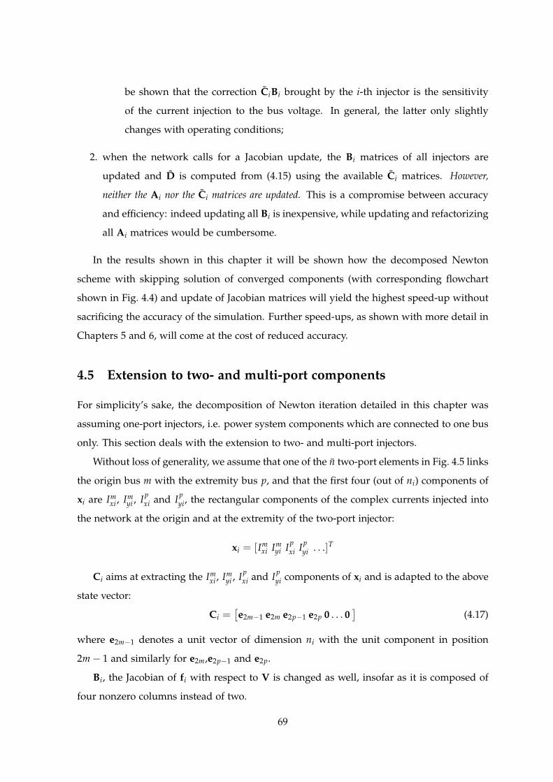
be shown that the correction CiBi brought by the i-th injector is the sensitivity
of the current injection to the bus voltage. In general, the latter only slightly
changes with operating conditions;
2. when the network calls for a Jacobian update, the Bi matrices of all injectors are
updated and D is computed from (4.15) using the available Ci matrices. However,
neither the Ai nor the Ci matrices are updated. This is a compromise between accuracy
and efficiency: indeed updating all Bi is inexpensive, while updating and refactorizing
all Ai matrices would be cumbersome.
In the results shown in this chapter it will be shown how the decomposed Newton
scheme with skipping solution of converged components (with corresponding flowchart
shown in Fig. 4.4) and update of Jacobian matrices will yield the highest speed-up without
sacrificing the accuracy of the simulation. Further speed-ups, as shown with more detail in
Chapters 5 and 6, will come at the cost of reduced accuracy.
4.5 Extension to two- and multi-port components
For simplicity’s sake, the decomposition of Newton iteration detailed in this chapter was
assuming one-port injectors, i.e. power system components which are connected to one bus
only. This section deals with the extension to two- and multi-port injectors.
Without loss of generality, we assume that one of the n two-port elements in Fig. 4.5 links
the origin bus m with the extremity bus p, and that the first four (out of ni) components of
xi are Imxi , Im
yi , Ipxi and Ip
yi, the rectangular components of the complex currents injected into
the network at the origin and at the extremity of the two-port injector:
xi = [Imxi Im
yi Ipxi Ip
yi . . .]T
Ci aims at extracting the Imxi , Im
yi , Ipxi and Ip
yi components of xi and is adapted to the above
state vector:
Ci =[e2m−1 e2m e2p−1 e2p 0 . . . 0
](4.17)
where e2m−1 denotes a unit vector of dimension ni with the unit component in position
2m− 1 and similarly for e2m,e2p−1 and e2p.
Bi, the Jacobian of fi with respect to V is changed as well, insofar as it is composed of
four nonzero columns instead of two.
69
p−th AC busAC network
i−th two−port injector
m−th AC bus
Ipxi Ip
yi
V = [Vx1 Vy1 . . . VxN VyN]T
i = 1, . . . , n
xi = [Imxi Im
yi Ipxi Ip
yi . . . ]T
. . .. . .
Imxi Im
yi
Vxp Vyp
Figure 4.5: Extension to two-port injectors
The Schur complement procedure is then the same as in the one-port case. The correc-
tion CiBi brought by the i-th injector into (4.15) only involves a (4× 4) sub-matrix centered
on the diagonal of D. In the one-port case the correction was added to four elements of D
which already existed: a shunt admittance at the bus of concern would bring one (2× 2)
correction at the same location. In the general case, however, the two-port injector brings
two (2× 2) corrections on the diagonal (2× 2) elements of the origin and the extremity bus,
along with two (2× 2) off-diagonal corrections, which would correspond to the Jacobian el-
ements brought by a network element connecting the same buses. Thus, D is structurally
symmetric also in the two-port case.
Two-port injectors allow to include black-box models of network elements in the general
BBD framework. It is the case, for instance, of HVDC links, that fit the general formulation
of Fig. 4.5, including the HVDC line itself as well as the converters and their controllers.
While the extension to n-port, for n arbitrary, is feasible, it is not useful. For instance, a
multi-terminal HVDC system connected to n AC buses can be decomposed into a set of n
two-port injectors, including the ACDC converters only, together with a purely DC network
including N DC buses and a number of DC lines, as sketched in Fig. 4.6.
To fit the general framework of phasor formulation, in which each voltage takes values
in R2, a fictitious second component of the voltage pair is introduced and set to zero for each
DC voltage. The same applies for current components. Within this framework, AC voltage
vector V and DC voltage vector VDC can be merged into a single vector and solved together.
It should be remarked that, as Fig. 4.6 shows, the resulting network is not connected.
70

m−th DC bus
Multi−terminal HVDC network
p−th AC bus
i−th ACDC two−port injector
AC network
V = [Vx1 Vy1 . . . VxN VyN]T
Vxp Vyp
Ipxi Ip
yi
i = 1, . . . , n
xi = [Imi 0 Ip
xi Ipyi . . . ]TIm
i
VDC = [VDC1 0 . . . VDC
N 0]T
VDCm
. . .. . .
Figure 4.6: Extension to multi-terminal HVDC networks
4.6 Scenari and results on Nordic32 system
This section gives details about the scenari that are simulated on the Nordic32 test system,
described in Section 2.4. The reference outputs have been obtained with an Integrated
dishonest Newton scheme (denoted as “I” in the plots). This section also provides the
results obtained by applying decomposition to the Nordic32 test system, on the whole set
of the proposed scenari.
Outputs have been obtained also with an accelerated decomposed dishonest Newton
scheme (denoted “A” in the plots) that makes use of the acceleration techniques proposed
in Sections 4.3 and 4.4. More details about this and the other solvers are given in Appendix
A.5. All evolutions obtained with scheme A are almost undistinguishable from those of
the benchmark scheme I. DTW distances between the outputs of scheme A and I (the latter
being the reference) are reported in Table 4.1. This section serves as a validation of the
techniques explained in this chapter; relevant results concerning the speed-up obtained,
while preserving accuracy, are detailed in the next sections.
4.6.1 Case N1
Case N1 is a line-tripping scenario. One circuit of line 1013-1014, located in the North area
(see Fig. 2.4), is tripped at t = 1 s. This short-term scenario is simulated until t = 30 s, when
71
most of the dynamics have died out.
The variables of interest for this case are:
• active power flow in the other circuit of line 1013-1014, taking over the tripped circuit
(Fig. 4.7);
• field voltage of generator g15, located in the Central area (Fig. 4.8).
The trajectories of output A with respect to output I are indistinguishable as confirmed
by the DTW distances shown in Table 4.1.
The differences between the outputs are within the chosen tolerance and can be appre-
ciated only when very small variations are plotted, such as in Fig. 4.8, that shows the field
voltage of generator g15, only marginally excited by the disturbance. An almost impercep-
tible difference is the slightly higher damping provided by scheme A, but let us highlight
the very small range of the over-damped oscillation: the corresponding DTW distances, in
Table 4.1, are in fact negligible.
4.6.2 Case N2
Case N2 is another line-tripping scenario: line 4043-4047, in the Central area, is tripped at
t = 1 s. The effect of this disturbance is stronger than in Case N1, leading to some long-
term dynamics, namely two LTC moves restoring the voltages at buses 4043 and 4046. The
simulation is stopped at t = 75 s, when the system approaches steady state.
The variables of interest for this case are:
• voltage at the distribution bus fed by 4043, which evolves under the effect of the line
outage and the LTC moves (Fig. 4.9);
• field voltage of and active power produced by generator g15, located in the Central
area, very close to the disturbance (Fig. 4.10 and 4.11, respectively).
4.6.3 Case N3
Case N3 is an unstable scenario initiated by the tripping of line 4032-4044, which is a crucial
element of the North-Central corridor, at t = 1 s. After some short-term oscillations, the
system evolves under the combined effects of the field current limitation imposed by several
72

120
140
160
180
200
220
0 5 10 15 20 25 30
active p
ow
er
(MW
)
t (s)
scheme I scheme A
Figure 4.7: Case N1: active power flow in one circuit of line 1013-1014
2.694
2.695
2.696
2.697
2.698
2.699
2.7
2.701
0 5 10 15 20 25 30
field
voltage (
pu)
t (s)
scheme I scheme A
Figure 4.8: Case N1: field voltage of generator g15
73

0.97
0.975
0.98
0.985
0.99
0.995
1
0 10 20 30 40 50 60 70
voltage m
agnitude (
pu)
t (s)
scheme I scheme A
Figure 4.9: Case N2: voltage at distribution bus fed by bus 4043
2.66
2.68
2.7
2.72
2.74
2.76
2.78
2.8
2.82
2.84
0 10 20 30 40 50 60 70
field
voltage (
pu)
t (s)
scheme I scheme A
Figure 4.10: Case N2: field voltage of generator g15
74

OELs and the LTCs trying to restore the distribution voltage. The trajectory is computed
until the collapse of the system, which takes place short before t = 180 s.
The variables of interest for this case are:
• voltage at transmission bus 1041, which shows the voltage evolution towards collapse
in the Central area (Fig. 4.12);
• speed deviation of generator g6, closely located to the initiating disturbance. This
machine has its field current limited at around t = 113 s and loses synchronism
towards the end of the simulation (Fig. 4.13). In this figure, the speed deviation of
generator g20 is also plotted in order to assess the loss of synchronism.
4.6.4 Case N4
Case N4 is an oscillatory unstable scenario. In normal conditions, three synchronous ma-
chines are equipped with power system stabilizers that provide damping torque even after
a wide variety of disturbances. For this case only, the three power system stabilizers are
disabled in order to obtain an oscillatory unstable evolution. The tripping of line 4061-4062,
at t = 1 s, triggers an oscillation in the South area which is simulated until the collapse of
the system, which takes place short before t = 25 s.
Case N4 allows to observe other small differences between the output A and the refer-
ence I, which may happen when the system is under stress. For instance, Fig. 4.14 shows the
field voltage of generator g17, strongly impacted by the disturbance. A small discrepancy
can be observed around t = 21 s, in the form of a slight delay.
Figure 4.15 provides the speed deviation of generator g17, directly affected by the initi-
ating disturbance, which loses synchronism towards the end of the simulation.
4.6.5 Case N5
Case N5 adds to the disturbance considered in case N3 a short circuit at bus 4032 lasting
from t = 0.9 s to t = 1 s. The long-term evolution is then similar to the one in case N3.
The variable of interest for this case is the voltage at transmission bus 1041, which shows
the voltage evolution towards collapse in the Central area (Fig. 4.16).
Table 4.1 also gives the DTW distances between the outputs of scheme A and I (the
latter being the reference). It further confirms that the accelerated decomposed dishonest
75

900
950
1000
1050
1100
1150
1200
0 10 20 30 40 50 60 70
active p
ow
er
(MW
)
t (s)
scheme I scheme A
Figure 4.11: Case N2: active power produced by generator g15
0.7
0.75
0.8
0.85
0.9
0.95
1
1.05
0 20 40 60 80 100 120 140 160 180
voltage m
agnitude (
pu)
t (s)
scheme I scheme A
Figure 4.12: Case N3: voltage at transmission bus 1041
76

0
0.002
0.004
0.006
0.008
0.01
0.012
0 20 40 60 80 100 120 140 160 180
speed d
evia
tion (
pu)
t (s)
g6, scheme I g6, scheme A g20, scheme I
Figure 4.13: Case N3: synchronous machine speed of generator g6
1
2
3
4
5
6
0 5 10 15 20 25
field
voltage (
pu)
t (s)
scheme I scheme A
Figure 4.14: Case N4: field voltage of generator g17
77

-0.01
0
0.01
0.02
0.03
0.04
0.05
0.06
0.07
0 5 10 15 20 25
speed d
evia
tion (
pu)
t (s)
scheme I scheme A
Figure 4.15: Case N4: synchronous machine speed of generator g17
0.5
0.6
0.7
0.8
0.9
1
1.1
0 20 40 60 80 100 120 140 160 180
voltage m
agnitude (
pu)
t (s)
scheme I scheme A
Figure 4.16: Case N5: voltage at transmission bus 1041
78

Newton scheme A (with skipping solution of converged components and update of Jacobian
matrices) preserves the accuracy of the simulated outputs, when compared to the integrated
scheme I.
Table 4.1: DTW distances
Fig. δ µ σ Unit4.7 0.0041 0.0001 0.0041 MW4.8 0.0001 0.0000 0.0001 pu4.9 0.0000 -0.0000 0.0000 pu4.10 0.0001 0.0000 0.0001 pu4.11 0.0182 -0.0009 0.0181 MW4.12 0.0001 0.0000 0.0001 pu4.13 0.0000 0.0000 0.0000 pu4.14 0.0211 -0.0033 0.0208 pu4.15 0.0002 0.0000 0.0002 pu4.16 0.0000 0.0000 0.0000 pu
4.7 Scenari and results on Hydro-Quebec system
This section details the scenari simulated on the Hydro-Quebec system, described in Section
2.5. The reference outputs have been obtained with an Integrated dishonest Newton scheme
(denoted as “I” in the plots).
Outputs have been obtained also with an accelerated decomposed dishonest Newton
scheme (denoted “A” in the plots) that makes use of the acceleration techniques proposed
in Sections 4.3 and 4.4. More details about this and the other solvers are given in Appendix
A.5.
4.7.1 Case Q1
Case Q1 is a short-term scenario which is initiated by a short circuit at bus 713, lasting
for 13 cycles (1 cycle at 60 Hz is 160 s), and cleared at t = 1 s by the opening of a series-
compensated 735-kV transmission line. This type of fault endangers rotor angle stability of
large northern hydro plants. The duration of the fault corresponds to a marginally stable
case. The evolution of the system is simulated up to t = 10 s.
The variables of interest for this case are:
• voltage at transmission bus 713, which undergoes wide oscillations after the short
circuit has been cleared (Fig. 4.17);
79
• speed deviations of synchronous machines 49 and 59, located in two different corri-
dors and swinging against each other (Fig. 4.18).
4.7.2 Case Q2
Case Q2 corresponds to a severe event that would lead to tripping generators with a pro-
duction of more than 1000 MW. The disturbance is applied at t = 1 s, and the resulting
transients are computed up to t = 100 s.
The variables of interest for this case are:
• speed deviation of the COI (see Appendix A.1, showing the average frequency evolu-
tion (Fig. 4.19);
• dynamic voltage correction produced by the power system stabilizer of a synchronous
condenser (machine 294) equipped with a low-frequency band aimed at damping
oscillations of the type shown in Fig. 4.19. This signal is applied to the AVR summing
junction of that machine (Fig. 4.20).
4.7.3 Case Q3
An even more severe generator tripping scenario is provided in case Q3, when three large
neighboring generators, producing altogether more than 2100 MW, are tripped at t = 1 s.
Figure 4.21 provides the speed deviation of the COI, showing that the spinning reserve
is exhausted and frequency cannot recover close to its nominal value. Underfrequency load
shedding would take place in such a case, but has not been modelled in this work.
4.7.4 Case Q4
Case Q4 is a 300 s evolution of voltage under the effect of MAIS (see Section 2.5) and LTCs,
after the tripping, at t = 1 s, of an important transmission line feeding the Montreal area
(where most of the load is located).
The variable of interest for this case is the voltage at transmission bus 702, provided in
Fig. 4.22.
It should be highlighted that the computed outputs are indistinguishable up to t = 32 s.
This scenario has a particular interest from the numerical point of view because the
computed evolution differs insofar as the switching of the first reactor, at bus 715, is de-
80

0.75
0.8
0.85
0.9
0.95
1
1.05
1.1
0 2 4 6 8 10
voltage m
agnitude (
pu)
t (s)
scheme I scheme A
Figure 4.17: Case Q1: zoom of the voltage evolution at faulted bus 713
-0.005
0
0.005
0.01
0.015
0.02
0.025
0.03
0 2 4 6 8 10
speed d
evia
tion (
pu)
t (s)
machine 49, scheme I machine 49, scheme A machine 59, scheme I
machine 59, scheme A
Figure 4.18: Case Q1: synchronous machine speed of generators 49 and 59
81

-0.007
-0.006
-0.005
-0.004
-0.003
-0.002
-0.001
0
0.001
0 20 40 60 80 100
speed d
evia
tion (
pu)
t (s)
scheme I scheme A
Figure 4.19: Case Q2: deviation of COI speed
-0.025
-0.02
-0.015
-0.01
-0.005
0
0.005
0.01
0 20 40 60 80 100
dvpss (
pu)
t (s)
scheme I scheme A
Figure 4.20: Case Q2: PSS signal of generator 294
82

-0.016
-0.014
-0.012
-0.01
-0.008
-0.006
-0.004
-0.002
0
0.002
0 20 40 60 80 100
speed d
evia
tion (
pu)
t (s)
scheme I scheme A
Figure 4.21: Case Q3: deviation of COI speed
0.95
0.955
0.96
0.965
0.97
0.975
0.98
0.985
0.99
0.995
1
0 50 100 150 200 250 300
voltage m
agnitude (
pu)
t (s)
scheme I scheme A
Figure 4.22: Case Q4: voltage at transmission bus 702
83

0.965
0.97
0.975
0.98
10 15 20 25 30 35 40
voltage m
agnitude (
pu)
t (s)
scheme I scheme A
MAIS switching threshold
Figure 4.23: Case Q4: zoom of the voltage evolution at transmission bus 715
layed in the simulation obtained with scheme A. Figure 4.23 shows a zoom of the voltage
evolution at bus 715 with the indication of the voltage threshold. The MAIS device switches
off the reactor if the voltage stays below that threshold for 9 s consecutively. In the output
computed with scheme I, the voltage of bus 715 crosses the threshold at t = 23 s and the
MAIS device acts at t = 32 s. The voltage computed with scheme A, on the other hand,
crosses the threshold at t = 25 s for the last time, leading to a trip at t = 34 s, although the
overall evolution up to that point can be considered accurate. A sort of “butterfly effect”
then produces a different switching time for the following three MAIS devices, leading to
apparently different system trajectories.
This case highlights the mismatch that can occur between marginally different cases,
when high impact discrete events, such as reactor tripping in this system, are taken into
account. It would be honest to claim that anyway both simulations can be considered
correct, as the acting MAIS are identified correctly, their action being merely shifted in time
as shown in Fig. 4.22. This fact is well recognized by TransEnergie engineers who consider
that a discrepancy by one reactor tripping is acceptable in practice.
84

0.96
0.965
0.97
0.975
0.98
0.985
0.99
0 50 100 150 200 250 300
voltage m
agnitude (
pu)
t (s)
scheme I scheme A
Figure 4.24: Case Q5: zoom of the voltage evolution at transmission bus 702
4.7.5 Case Q5
Case Q5 considers a short circuit near bus 702 lasting for 7 cycles, that is cleared by opening
the same transmission line as in case Q4. The long-term evolution is then similar to the one
in case Q4. Figure 4.24 shows the zoomed evolution of voltage at faulted bus 702. In this
simulation there is no marginally switching MAIS device, thus the computed outputs are
indistinguishable.
4.7.6 Computational effort
Table 4.2 summarizes the computing times obtained with the application of scheme A with
respect to the benchmark provided by scheme I. It should be kept in mind that the speedup
comes at no cost concerning the overall accuracy of the simulated outputs.
Table 4.2: CPU times (s)
Case Scheme I Scheme AQ1 11.11 5.93Q2 35.84 11.91Q3 27.89 13.16Q4 60.16 30.55Q5 61.34 34.36
85
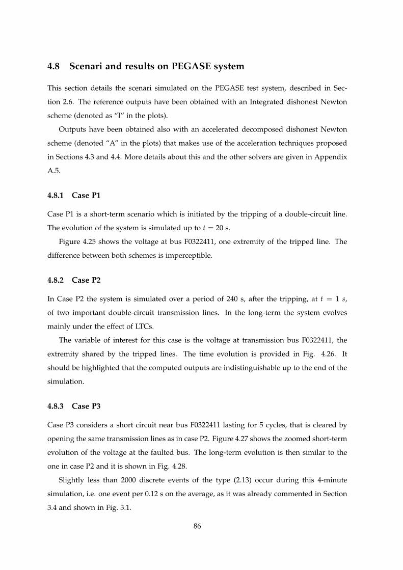
4.8 Scenari and results on PEGASE system
This section details the scenari simulated on the PEGASE test system, described in Sec-
tion 2.6. The reference outputs have been obtained with an Integrated dishonest Newton
scheme (denoted as “I” in the plots).
Outputs have been obtained also with an accelerated decomposed dishonest Newton
scheme (denoted “A” in the plots) that makes use of the acceleration techniques proposed
in Sections 4.3 and 4.4. More details about this and the other solvers are given in Appendix
A.5.
4.8.1 Case P1
Case P1 is a short-term scenario which is initiated by the tripping of a double-circuit line.
The evolution of the system is simulated up to t = 20 s.
Figure 4.25 shows the voltage at bus F0322411, one extremity of the tripped line. The
difference between both schemes is imperceptible.
4.8.2 Case P2
In Case P2 the system is simulated over a period of 240 s, after the tripping, at t = 1 s,
of two important double-circuit transmission lines. In the long-term the system evolves
mainly under the effect of LTCs.
The variable of interest for this case is the voltage at transmission bus F0322411, the
extremity shared by the tripped lines. The time evolution is provided in Fig. 4.26. It
should be highlighted that the computed outputs are indistinguishable up to the end of the
simulation.
4.8.3 Case P3
Case P3 considers a short circuit near bus F0322411 lasting for 5 cycles, that is cleared by
opening the same transmission lines as in case P2. Figure 4.27 shows the zoomed short-term
evolution of the voltage at the faulted bus. The long-term evolution is then similar to the
one in case P2 and it is shown in Fig. 4.28.
Slightly less than 2000 discrete events of the type (2.13) occur during this 4-minute
simulation, i.e. one event per 0.12 s on the average, as it was already commented in Section
3.4 and shown in Fig. 3.1.
86

0.98
0.99
1
1.01
1.02
1.03
1.04
1.05
0 5 10 15 20
voltage m
agnitude (
pu)
t (s)
scheme I scheme A
Figure 4.25: Case P1: voltage at transmission bus F0322411
0.99
1
1.01
1.02
1.03
1.04
1.05
0 50 100 150 200
voltage m
agnitude (
pu)
t (s)
scheme I scheme A
Figure 4.26: Case P2: voltage at transmission bus F0322411
87
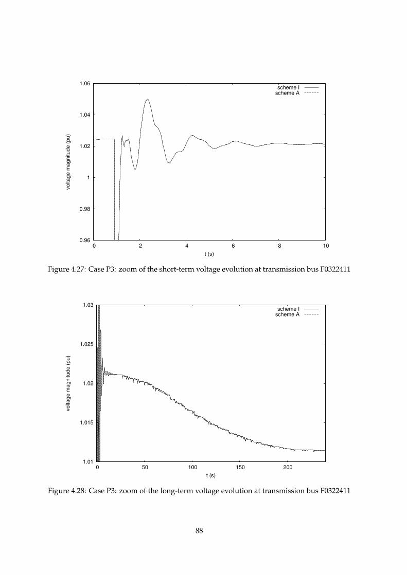
0.96
0.98
1
1.02
1.04
1.06
0 2 4 6 8 10
voltage m
agnitude (
pu)
t (s)
scheme I scheme A
Figure 4.27: Case P3: zoom of the short-term voltage evolution at transmission bus F0322411
1.01
1.015
1.02
1.025
1.03
0 50 100 150 200
voltage m
agnitude (
pu)
t (s)
scheme I scheme A
Figure 4.28: Case P3: zoom of the long-term voltage evolution at transmission bus F0322411
88
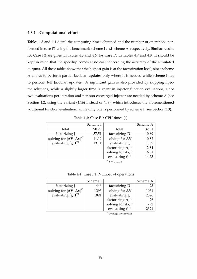
4.8.4 Computational effort
Tables 4.3 and 4.4 detail the computing times obtained and the number of operations per-
formed in case P1 using the benchmark scheme I and scheme A, respectively. Similar results
for Case P2 are given in Tables 4.5 and 4.6, for Case P3 in Tables 4.7 and 4.8. It should be
kept in mind that the speedup comes at no cost concerning the accuracy of the simulated
outputs. All these tables show that the highest gain is at the factorization level, since scheme
A allows to perform partial Jacobian updates only where it is needed while scheme I has
to perform full Jacobian updates. A significant gain is also provided by skipping injec-
tor solutions, while a slightly larger time is spent in injector function evaluations, since
two evaluations per iteration and per non-converged injector are needed by scheme A (see
Section 4.2, using the variant (4.16) instead of (4.9), which introduces the aforementioned
additional function evaluation) while only one is performed by scheme I (see Section 3.3).
Table 4.3: Case P1: CPU times (s)
Scheme I Scheme Atotal 90.29 total 32.81
factorizing J 57.51 factorizing D 0.69solving for [∆V ∆x]T 11.19 solving for ∆V 0.82
evaluating [g f]T 13.11 evaluating g 1.97factorizing Ai
? 2.84solving for ∆xi
? 6.51evaluating fi
? 14.75? i = 1, . . . , n
Table 4.4: Case P1: Number of operations
Scheme I Scheme Afactorizing J 446 factorizing D 25
solving for [∆V ∆x]T 1393 solving for ∆V 1031evaluating [g f]T 1891 evaluating g 2326
factorizing Ai? 26
solving for ∆xi? 792
evaluating fi? 2321
? average per injector
89
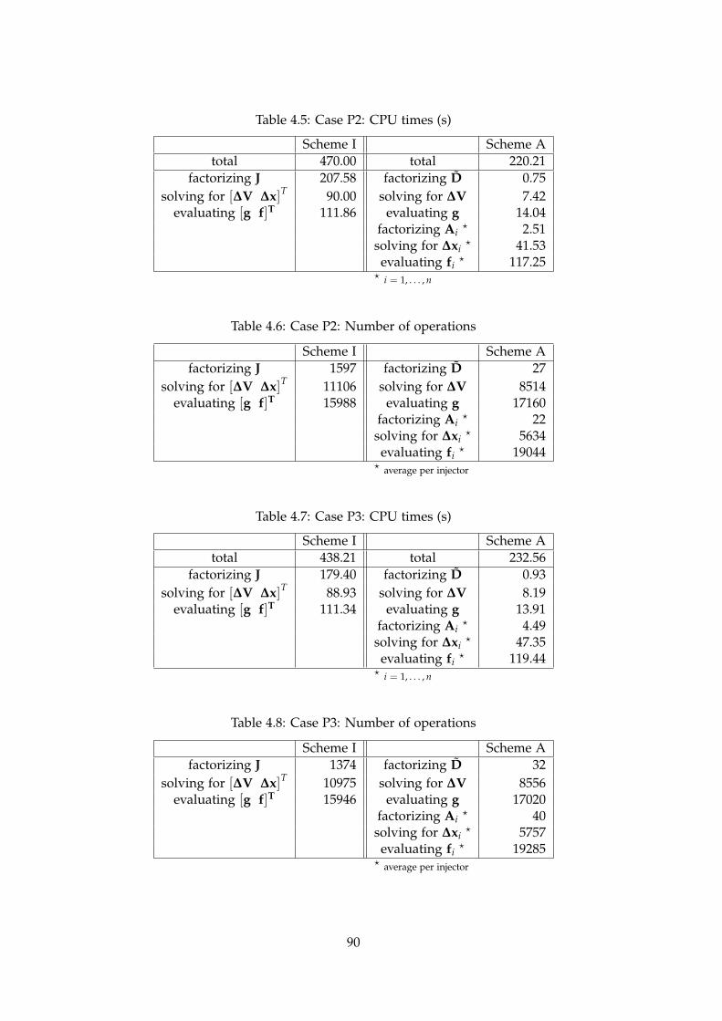
Table 4.5: Case P2: CPU times (s)
Scheme I Scheme Atotal 470.00 total 220.21
factorizing J 207.58 factorizing D 0.75solving for [∆V ∆x]T 90.00 solving for ∆V 7.42
evaluating [g f]T 111.86 evaluating g 14.04factorizing Ai
? 2.51solving for ∆xi
? 41.53evaluating fi
? 117.25? i = 1, . . . , n
Table 4.6: Case P2: Number of operations
Scheme I Scheme Afactorizing J 1597 factorizing D 27
solving for [∆V ∆x]T 11106 solving for ∆V 8514evaluating [g f]T 15988 evaluating g 17160
factorizing Ai? 22
solving for ∆xi? 5634
evaluating fi? 19044
? average per injector
Table 4.7: Case P3: CPU times (s)
Scheme I Scheme Atotal 438.21 total 232.56
factorizing J 179.40 factorizing D 0.93solving for [∆V ∆x]T 88.93 solving for ∆V 8.19
evaluating [g f]T 111.34 evaluating g 13.91factorizing Ai
? 4.49solving for ∆xi
? 47.35evaluating fi
? 119.44? i = 1, . . . , n
Table 4.8: Case P3: Number of operations
Scheme I Scheme Afactorizing J 1374 factorizing D 32
solving for [∆V ∆x]T 10975 solving for ∆V 8556evaluating [g f]T 15946 evaluating g 17020
factorizing Ai? 40
solving for ∆xi? 5757
evaluating fi? 19285
? average per injector
90

Figure 4.29 shows the number of injector solutions per step in scheme I. The first 10 s are
not shown because deemed less interesting. With scheme I, solutions are computed for all
injectors at each Newton iteration. Thus, given that the number of injectors of this system
is n = 10694, this plot only shows values in multiples of n: for most of the steps, 1,2,3 or
4 iterations are enough to solve the system of equations up to the desired tolerance. For
legibility, values larger than 50000 are not displayed, although present at a few time steps
with more difficult convergence (corresponding to 5,6 and 7 iterations).
Figure 4.30 shows the number of injector solutions per step in scheme A. The lower
bound of the plotted values is again n, since at least one iteration per injector is performed
at each step. As in scheme I, some of the injectors need up to 4, or in some cases even 6
iterations in order to be solved: as expected, however, not all the injectors need the same
number of iterations, as many are already solved up to convergence with just one Newton
iteration.
The small subset of injectors that require more iterations is also responsible for the much
higher number of Jacobian factorization in scheme I with respect to scheme A: indeed, while
in scheme A a slow convergence of one injector forces to update only its own Jacobian
matrix, in scheme I a slow convergence of just one injector (or, for that matter, even of just
one equation inside one injector) slows down the convergence of the whole system, many
times forcing the solver to perform a full Jacobian update.
In integrated schemes, this problem can be easily avoided at some risk by temporarily
disabling the infinite-norm or adopting a varying-order-norm, as discussed in Section 3.3:
a few large mismatches would then be shaded by the majority of small mismatches, and
considered converged before triggering Jacobian updates. In the author’s opinion, however,
the different rate of convergence of variables is inherent in large power systems made up
of many components which experience different level of activity, and thus converge each at
its own speed. This fact provides valid arguments in favor of decomposition for large-scale
power systems, where the natural choice of the infinite-norm may be kept at (almost) no
cost.
4.9 Chapter conclusion
The most important contributions of this chapter are the acceleration techniques made pos-
sible by decomposing the Newton method algorithm. The skipping solution of converged
91
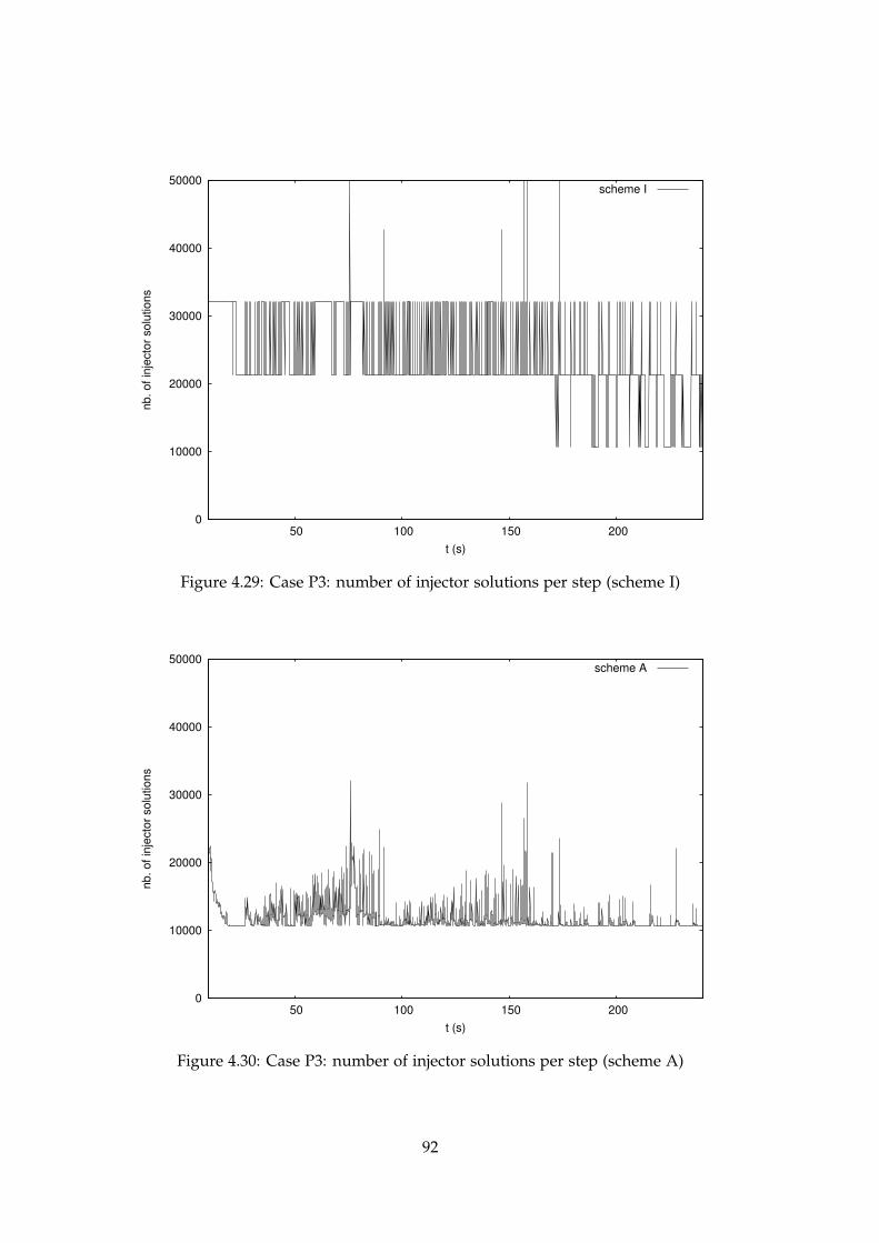
0
10000
20000
30000
40000
50000
50 100 150 200
nb. of in
jecto
r solu
tions
t (s)
scheme I
Figure 4.29: Case P3: number of injector solutions per step (scheme I)
0
10000
20000
30000
40000
50000
50 100 150 200
nb. of in
jecto
r solu
tions
t (s)
scheme A
Figure 4.30: Case P3: number of injector solutions per step (scheme A)
92

components detailed in Section 4.3 and the partial Jacobian update strategy detailed in Sec-
tion 4.4 bring a speed-up ranging between 2 and 3. This speed-up comes at no cost, since
the accuracy of the computed outputs is preserved.
93


Chapter5
Relaxing accuracy in space
Divide et impera 1
A brief review of spatial accuracy relaxation methods opens this chapter, with a partic-
ular emphasis on localization methods for power flow and latency exploitation in electronic
circuits. The idea of localization, borrowed from the power flow problem, but novel in its
application to dynamic simulation is presented and implemented thanks to the BBD de-
composition detailed in Chapter 4. The influence of the latency tolerance is discussed and
results are presented on the three test systems showing that the computational effort can be
reduced gradually, along with the accuracy of the simulated outputs, especially for system
components which are marginally participating to the system dynamics.
5.1 Spatial accuracy relaxation in literature
The concept of localization results from the observation of the limited effect that a vast
majority of disturbances has over a large system, and it has been used extensively both in
power systems [Bra93] and in electronic circuits [HSV81].
This phenomenon has been exploited since the dawn of power system numerical sim-
ulation, although it was not mentioned under the name of localization. For instance, the
network reduction leading to the so-called Ward equivalents [War49], which is simply the
1Divide and rule. Apocryphal, attributed to Gaius Julius Caesar and Napoleon Bonaparte among others.
95

Gaussian elimination of the external buses in the system admittance matrix equation, has
long been considered the standard for static equivalencing [MDGS79]. The main hypothe-
sis justifying the widespread use of equivalencing is that the role of the external network
is marginal for the evaluation of the phenomena of interest; historically its adoption was
motivated by computational efficiency reasons, especially in the context of online security
assessment [WM83], while recently the use of external equivalents in order to deal with
confidentiality issues in data exchanges between system operators has also been advocated
[FGWVC09].
Equivalents have been also used in dynamic simulation. As regards electromechanical
oscillations, the techniques used [ANL+12] can be roughly classified into (i) modal methods
[Cho82], based on the linearized state-space model, (ii) coherency methods [GP78], based
on clustering the system components according to their response to a given disturbance
and (iii) measurement methods [YES81], based on system identification techniques applied
to recorded or simulated responses.
The main drawback of techniques based on equivalencing is that the model simplifica-
tion is performed at the beginning of the simulation and it cannot, in principle, be changed
to suit different scenari. Furthermore, a universal equivalent that would be valid for all
power system dynamic phenomena, to the author’s knowledge is still to be found.
Contingency analysis has been another area of application of localization concepts and
a step forward towards an adaptive use of spatial relaxation. Several approaches ex-
ploited the limited widespread of contingencies in order to compute the corresponding
post-disturbance state without taking into account the whole system: among those ap-
proaches let us mention concentric relaxation [ZWP80], bound estimates method [Gal84]
and bounding method both for DC [Bra88] and AC [BL89] power flow computations.
The approaches listed above, while allowing to vary the degree of accuracy relaxation to
match the different scenari, still suffer from the fact that different reduced systems have to
be computed as the affected area changes, bringing additional overhead if a direct method,
such as the Newton method, is used for the solution of the resulting system of equations.
The algorithms based on sparse vector method [TBC85] tackle this problem by allowing a
partial solution of the whole system, i.e. a variation of the relaxation degree without the
need of restructuring the underlying systems of equations. Successive refinements, such
as the zero mismatch approach [BT89], the approximate sparse vector method [BET91] and
adaptive localization [EPT92] improved the original approach, while being still limited to
96

the power flow problem, though.
To our knowledge, extension of sparse vector approaches to power system dynamics,
although intuitively appealing, has not been investigated. The localization algorithm de-
scribed in Section 5.2 bears the spirit of those approaches insofar as it allows a varying
degree of accuracy relaxation, while keeping the problem structure intact.
Variable partitioning multi-rate methods [CC08], which adapt the subdomains accord-
ing to the “level of activity” of the variables involved, are probably the most advanced
exploitation of the localization property in power system dynamics. In this approach, vari-
ables are divided in different subsets which are solved with different time steps. The two
main drawbacks are that (i) the method suffers from degradation of convergence due to
decomposition and interface problems inherent to relaxation methods in general, especially
when there is no overlap between subdomains [TW05], and (ii) the decomposition is based
on the “dynamic” activity of variables, not on their location, resulting in subsets which,
in general, may not be contiguous. For this last reason this method cannot be fully clas-
sified as a spatial relaxation of accuracy, as will be further discussed in Chapter 6. The
decomposition into network and injectors considered in this work is free from the above
drawbacks.
In electronic circuits simulations, localization is referred to as latency. It has been ex-
ploited for quite some time. The high popularity of this method in electronics can be
explained by the nature of the involved circuits which are composed of simple repetitive
subnetworks [RSVH79]. Especially in digital circuits, the latency state of a component can
be determined rather easily compared to power systems; moreover, subnetworks are latent
for most of the simulation. As it will be detailed in Section 5.3, the application of localiza-
tion to power systems requires a more careful test to detect the latent state of a component,
by the comparison of its level of activity to a latency tolerance.
5.2 Localization in the decomposed Newton scheme
The idea behind localization is to solve only a subset of injectors, identified as active, and
skip solution of the other ones, identified as latent.
The active injectors are solved with the same accuracy as for a detailed simulation.
Furthermore, with the techniques presented in Chapter 4, Eqs. (4.9) are solved more times
for injectors with higher dynamic response. On the other hand, for the latent ones, Eqs.
97

(4.9) will not be solved at all; in fact, their functions fi will not even be computed. Note that
the whole network will still be solved according to (4.11).
We found it appropriate to replace a latent injector by a linear approximation between its
current and voltage. This approximation is obtained from (4.9), assuming that the injector
internal dynamics are negligible, i.e.
fi(xk−1i , zi, Vk−1) ' 0
Under this approximation, (4.9) becomes:
Ai∆xi ' −Bi∆V (5.1)
from which ∆xi is easily obtained:
∆xi ' −A−1i Bi∆V (5.2)
The variation of the current components is obtained by pre-multiplying (5.2) by Ci:
∆Ixi
∆Iyi
0...
0
= Ci∆xi ' −CiA−1
i Bi∆V = −CiBi∆V (5.3)
which is the sought linear relation between current and voltage. Extracting the nonzero
elements of (5.3) yields: ∆Ixi
∆Iyi
= −Si
∆Vxi
∆Vyi
(5.4)
where the (2× 2) matrix Si contains the 4 nonzero elements of CiBi.
Since the above relations are linear, their variations can be rewritten around a lineariza-
tion point at an arbitrary instant t∗i , characterized by current values[
Ixi(t∗i ) Iyi(t∗i )]T
and voltage values[
Vxi(t∗i ) Vyi(t∗i )]T
, without loss of generality: Ixi
Iyi
=
Ixi(t∗i )
Iyi(t∗i )
− Si
Vxi −Vxi(t∗i )
Vyi −Vyi(t∗i )
(5.5)
Going back to the full state vector xi of the injector, the above formula can be rewritten
in compact form as
xi = x∗i − CiBi∆V∗ (5.6)
98

where x∗i is the full state vector value at the arbitrary instant t∗i and ∆V∗ is defined as
V−V∗.
Note that the linear formula (5.5) is simple and merely involves matrix multiplications.
It does not require a Newton solution, which is precisely the objective for latent injectors.
Furthermore, one important feature is that the correction −CiBi brought by the i-th
injector to the D matrix is the same whether the injector is active or latent. In other words,
when an injector switches from active to latent or viceversa, it does not modify the D matrix.
The latter need not be updated, and the convergence of the Newton method is not degraded
by re-using the same matrix in a “dishonest” way.
If the i-th injector is latent, its current components Ixi and Iyi are updated according
to (5.3) but the other components of its state vector xi are no longer updated. There is
an exception, however, for synchronous machines: it is assumed that a latent synchronous
machine swings coherently with the center of inertia of the system. Hence, at each time
step, its rotor speed ω is set to ωcoi, the angular speed of the center of inertia.
In the sequel, the resulting algorithm is referred to as localized Newton scheme. The
corresponding flowchart is shown in Fig. 5.1, which should be compared to Figs. 4.3 and
4.4.
5.3 Latency detection algorithm
Which injectors are latent and which ones are active cannot be decided a priori because it
depends on the simulated disturbance. This is a major advantage of the proposed method
with respect to equivalencing techniques. Furthermore, it may happen that an injector
changes from active to latent after some transients have died out, then switches back to
active under the effect of the system evolution.
We define the linearization instant t∗i as the last time the i-th injector changed from active
to latent and was replaced by the linear model (5.3) or its equivalent relation (5.5). At the
beginning of the simulation, t∗i is initialized to zero for all injectors.
As a result of extensive tests, the following latency identification rules were found the
most satisfactory:
1. at the beginning of the simulation or after a user-imposed event: all injectors are
classified active (in the absence of information regarding the dynamics that will be
excited);
99

injectors
network
Y
N
Y
N
N
Y
N
xki = xk−1
i + ∆xki
N
solve Ai∆xki = −fi(xk−1
i , Vk)
k := k + 1
xki = x∗i +
k := k + 1
|CiBi∆V∗| εL<
Y
stop
all injectors converged?
Y
||g(xki , ..., xk
n, Vk)||∞ < εg
i := i + 1
i ≤ n
injector i converged?
injector i latent?
k := 1
−CiBi∆V∗
−∑ Cifi(xk−1i , Vk−1)
solve D∆Vk = −g(xk−11 , ..., xk−1
n , Vk−1)
Vk = Vk−1 + ∆Vk
N
i := 1
Y
start
Figure 5.1: Localized Newton scheme
100
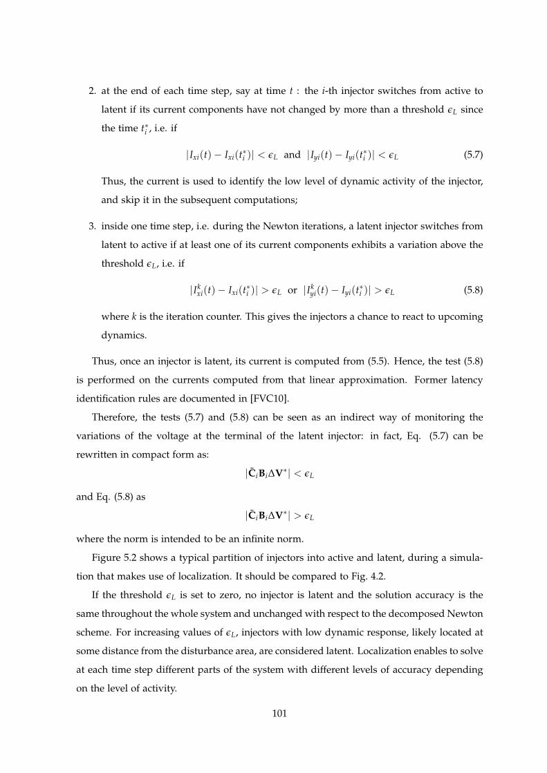
2. at the end of each time step, say at time t : the i-th injector switches from active to
latent if its current components have not changed by more than a threshold εL since
the time t∗i , i.e. if
|Ixi(t)− Ixi(t∗i )| < εL and |Iyi(t)− Iyi(t∗i )| < εL (5.7)
Thus, the current is used to identify the low level of dynamic activity of the injector,
and skip it in the subsequent computations;
3. inside one time step, i.e. during the Newton iterations, a latent injector switches from
latent to active if at least one of its current components exhibits a variation above the
threshold εL, i.e. if
|Ikxi(t)− Ixi(t∗i )| > εL or |Ik
yi(t)− Iyi(t∗i )| > εL (5.8)
where k is the iteration counter. This gives the injectors a chance to react to upcoming
dynamics.
Thus, once an injector is latent, its current is computed from (5.5). Hence, the test (5.8)
is performed on the currents computed from that linear approximation. Former latency
identification rules are documented in [FVC10].
Therefore, the tests (5.7) and (5.8) can be seen as an indirect way of monitoring the
variations of the voltage at the terminal of the latent injector: in fact, Eq. (5.7) can be
rewritten in compact form as:
|CiBi∆V∗| < εL
and Eq. (5.8) as
|CiBi∆V∗| > εL
where the norm is intended to be an infinite norm.
Figure 5.2 shows a typical partition of injectors into active and latent, during a simula-
tion that makes use of localization. It should be compared to Fig. 4.2.
If the threshold εL is set to zero, no injector is latent and the solution accuracy is the
same throughout the whole system and unchanged with respect to the decomposed Newton
scheme. For increasing values of εL, injectors with low dynamic response, likely located at
some distance from the disturbance area, are considered latent. Localization enables to solve
at each time step different parts of the system with different levels of accuracy depending
on the level of activity.
101

latent injectors
j−th bus
i−th injector
network
active injectors
. . .
V = [Vx1 Vy1 . . . VxN VyN]T
Vxj Vyj
Ixi Iyi
M i = 1, . . . , n
xi = [Ixi Iyi . . . ]T
xi = x∗i − CiBi∆V∗0 = fi(xi, zi, V)
. . .
Figure 5.2: Partition of injectors into active and latent
5.4 Localization results on Nordic32 system
This section illustrates how localization works in practice, in the scenari described in Section
4.6. The effect of localization on such a small system is limited: for this reason only Cases
N1 and N2 will be shown in detail; in the other cases, which end with a collapse of the
system, localization is exploited only marginally. The outputs have been obtained with
a localized dishonest Newton scheme, denoted “L” in the plots, using different latency
tolerances εL. Localization has not been used during the first half second after a user-
imposed disturbance. More details about this and the other solvers are given in Appendix
A.5. Only some representative curves are shown, since the trajectories obtained with scheme
L are very close to the benchmark trajectories of scheme I in all cases, at least in the DTW
sense (i.e. without penalizing too much small delays). The reported DTW distances are
computed on the output given by scheme L with respect to the one given by scheme I, and
are given in Table 5.1. Relevant results concerning the speed-up are detailed in the next
sections, on Hydro-Quebec and PEGASE systems, which, due to their larger size, profit
more from localization.
5.4.1 Case N1
Figure 5.3 shows the active power flow in the other circuit of line 1013-1014. It can be seen
that the simulated response is accurate whatever the value of the latency tolerance. With
102

εL = 0.001, 23 injectors out of 42 are latent for most of the simulation. Increasing the latency
tolerance brings this number up to 28, for εL = 0.002, and 36 for εL = 0.01.
Figure 5.4 depicts the field voltage of generator g15, only marginally excited by the
disturbance. The instants where the generator has switched from active to latent are easily
identified from the horizontal line. The higher the value of εL, the sooner g15 becomes
latent and its field voltage evolution shows a straight line. At first glance, the evolution
provided by setting εL = 0.01 does not look accurate; however, bearing in mind the small
range of values of the displayed output, it is clear that the approximation brought by even
the highest latency tolerance is acceptable for many practical applications.
5.4.2 Case N2
Case N2 involves a long-term scenario. Figure 5.5 shows the voltage at the distribution bus
fed by 4043. The two LTC moves of the transformers, at around t = 38 s and t = 46 s, are
both shifted in time for εL = 0.01, but this does not significantly impact the overall evolution
of the system. For εL = 0.002, only a single LTC move only is delayed, while εL = 0.001
returns no difference with respect to the benchmark.
As in Case N1, a progressively larger number of injectors becomes latent with the in-
crease of the latency tolerance.
The field voltage and active power of generator g15 are shown in Figs. 5.6 and 5.7,
respectively. This machine is very close to the disturbance, and for εL = 0.01 it only becomes
latent towards the end of the simulation. Tighter latency tolerances do not allow it to switch
to latent. For increasing latency tolerances, the initial oscillations tend to be over-damped,
as the increasing values of σ in Table 5.1 also indicate. The simulated outputs, overall, are
accurate, as shown by the δ values in Table 5.1: the DTW distance, in fact, allows catching
the similar pattern of outputs, without over-penalizing the delays as the Euclidean distance
would do in this case.
5.4.3 Other cases
Cases N3, N4 and N5, which all end up collapse, offer less possibilities to exploit localiza-
tion. Nonetheless, their output are still accurate, as shown by the DTW distances given in
Table 5.1.
103

120
140
160
180
200
220
0 5 10 15 20 25 30
active p
ow
er
(MW
)
t (s)
scheme I scheme L, epsilonL=0.001 scheme L, epsilonL=0.02 scheme L, epsilonL=0.01
Figure 5.3: Case N1: active power flow in one circuit of line 1013-1014
2.694
2.695
2.696
2.697
2.698
2.699
2.7
2.701
0 5 10 15 20 25 30
field
voltage (
pu)
t (s)
scheme I scheme L, epsilonL=0.001 scheme L, epsilonL=0.02 scheme L, epsilonL=0.01
Figure 5.4: Case N1: field voltage of generator g15
104

0.97
0.975
0.98
0.985
0.99
0.995
1
0 10 20 30 40 50 60 70
voltage m
agnitude (
pu)
t (s)
scheme I scheme L, epsilonL=0.001 scheme L, epsilonL=0.02 scheme L, epsilonL=0.01
Figure 5.5: Case N2: voltage at distribution bus fed by bus 4043
2.66
2.68
2.7
2.72
2.74
2.76
2.78
2.8
2.82
2.84
0 10 20 30 40 50 60 70
field
voltage (
pu)
t (s)
scheme I scheme L, epsilonL=0.001 scheme L, epsilonL=0.02 scheme L, epsilonL=0.01
Figure 5.6: Case N2: field voltage of generator g15
105

900
950
1000
1050
1100
1150
1200
0 10 20 30 40 50 60 70
active p
ow
er
(MW
)
t (s)
scheme I scheme L, epsilonL=0.001 scheme L, epsilonL=0.02 scheme L, epsilonL=0.01
Figure 5.7: Case N2: active power produced by generator g15
1
2
3
4
5
6
0 5 10 15 20 25
field
voltage (
pu)
t (s)
scheme I scheme L, epsilonL=0.001 scheme L, epsilonL=0.02 scheme L, epsilonL=0.01
Figure 5.8: Case N4: field voltage of generator g17
106
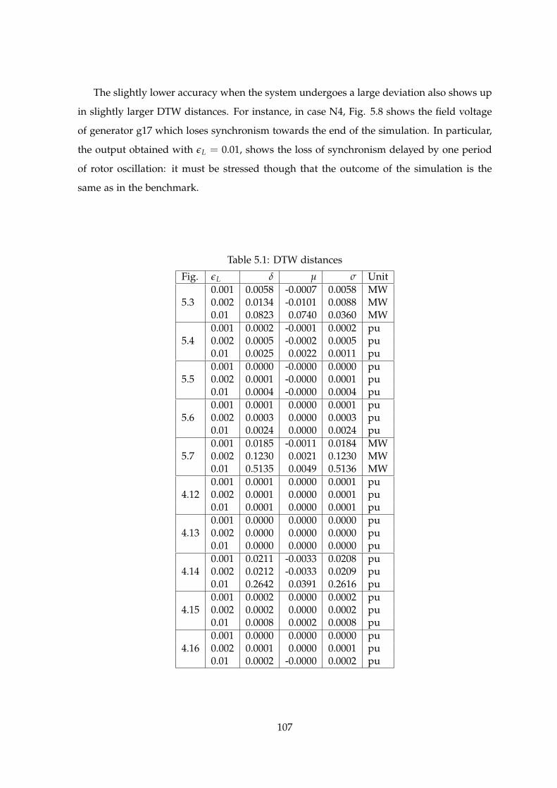
The slightly lower accuracy when the system undergoes a large deviation also shows up
in slightly larger DTW distances. For instance, in case N4, Fig. 5.8 shows the field voltage
of generator g17 which loses synchronism towards the end of the simulation. In particular,
the output obtained with εL = 0.01, shows the loss of synchronism delayed by one period
of rotor oscillation: it must be stressed though that the outcome of the simulation is the
same as in the benchmark.
Table 5.1: DTW distances
Fig. εL δ µ σ Unit0.001 0.0058 -0.0007 0.0058 MW
5.3 0.002 0.0134 -0.0101 0.0088 MW0.01 0.0823 0.0740 0.0360 MW0.001 0.0002 -0.0001 0.0002 pu
5.4 0.002 0.0005 -0.0002 0.0005 pu0.01 0.0025 0.0022 0.0011 pu0.001 0.0000 -0.0000 0.0000 pu
5.5 0.002 0.0001 -0.0000 0.0001 pu0.01 0.0004 -0.0000 0.0004 pu0.001 0.0001 0.0000 0.0001 pu
5.6 0.002 0.0003 0.0000 0.0003 pu0.01 0.0024 0.0000 0.0024 pu0.001 0.0185 -0.0011 0.0184 MW
5.7 0.002 0.1230 0.0021 0.1230 MW0.01 0.5135 0.0049 0.5136 MW0.001 0.0001 0.0000 0.0001 pu
4.12 0.002 0.0001 0.0000 0.0001 pu0.01 0.0001 0.0000 0.0001 pu0.001 0.0000 0.0000 0.0000 pu
4.13 0.002 0.0000 0.0000 0.0000 pu0.01 0.0000 0.0000 0.0000 pu0.001 0.0211 -0.0033 0.0208 pu
4.14 0.002 0.0212 -0.0033 0.0209 pu0.01 0.2642 0.0391 0.2616 pu0.001 0.0002 0.0000 0.0002 pu
4.15 0.002 0.0002 0.0000 0.0002 pu0.01 0.0008 0.0002 0.0008 pu0.001 0.0000 0.0000 0.0000 pu
4.16 0.002 0.0001 0.0000 0.0001 pu0.01 0.0002 -0.0000 0.0002 pu
107

5.5 Localization results on Hydro-Quebec system
In this section, localization techniques are applied to the scenari described in Section 4.7.
The gain in computing time introduced by localization is somewhat limited on this “medium
size” model of a system which operates isolated and is subject to large disturbances. The
outputs have been obtained with a localized dishonest Newton scheme, denoted “L” in
the plots, using different latency tolerances εL. Localization has not been used during the
first three seconds after a user-imposed disturbance. More details about this and the other
solvers are given in Appendix A.5.
5.5.1 Case Q2
Figure 5.9 shows the speed deviation of the COI, after the loss of active power generation.
The curves computed with scheme L are increasingly closer to the benchmark for smaller
εL.
5.5.2 Case Q4
Case Q4 involves the long-term evolution of the system under the antagonistic effects of
MAIS and LTCs. The voltage at transmission bus 702 is provided in Fig. 5.10.
The differences between the various simulated outputs are due to the marginally delayed
switchings of the first reactor, located at bus 715, as already discussed in Section 4.7.4. These
differences are definitely negligible for practical applications. The curve computed by using
the smallest tolerance εL is indistinguishable from the benchmark though.
5.5.3 Computational effort
Table 5.2 gives the CPU times to evaluate the speed-up brought by scheme L with various
latency tolerances εL in all scenari. It confirms that some gain can be obtained, especially
in long-term cases. The largest advantages of scheme L, however, will be shown in the
next section, on the PEGASE system, whose size allows a more profitable exploitation of
localization. The CPU times of scheme A are reported for comparison, since scheme L, for
εL → 0, is identical to scheme A.
While Cases Q2, Q3 and Q4 show an increasing speed-up for increasing εL, as expected,
Cases Q1 and Q5 offer some perspective over the limits of application of localization.
108

-0.007
-0.006
-0.005
-0.004
-0.003
-0.002
-0.001
0
0.001
0 20 40 60 80 100
speed d
evia
tion (
pu)
t (s)
scheme I scheme L, epsilon_L=0.001 scheme L, epsilon_L=0.025 scheme L, epsilon_L=0.01
Figure 5.9: Case Q2: deviation of COI speed
0.95
0.955
0.96
0.965
0.97
0.975
0.98
0.985
0.99
0.995
1
0 50 100 150 200 250 300
voltage m
agnitude (
pu)
t (s)
scheme I scheme L, epsilon_L=0.001
scheme L, epsilon_L=0.0025 scheme L, epsilon_L=0.01
Figure 5.10: Case Q4: voltage at transmission bus 702
109

Table 5.2: CPU times (s)
Case Scheme I Scheme A Scheme L Scheme L Scheme LεL = 0.001 εL = 0.0025 εL = 0.01
Q1 11.11 5.93 6.04 5.74 5.72Q2 35.84 11.91 11.06 9.46 8.30Q3 27.89 13.16 12.19 11.45 9.93Q4 60.16 30.55 28.51 26.96 23.43Q5 61.34 34.36 32.80 31.26 32.19
5.5.4 Other cases
Case Q1 shows even a degradation of performance, with respect to scheme A, when the
strictest latency tolerance is used: in fact this is a short-term scenario simulating a fault
and the subsequent transients during which, most probably, only a really small part of the
system, if any, can be considered latent. For increasing tolerances, though, some speed-up
is found.
Case Q5, on the other hand, shows that increasing εL brings a more efficient simulation
up to some threshold, where the slow-down due to approximations brought by latency
eventually offset the speed-up. For this case for instance, a value of εL larger than 0.0025 is
not useful.
5.6 Localization results on PEGASE system
In this section, localization techniques are applied to the scenari described in Section 4.8.
Expectedly, on the PEGASE system, the gain in computing time brought by localization is
the highest among the three systems considered in this work. The outputs have been ob-
tained with a localized dishonest Newton scheme, denoted “L” in the plots, using different
latency tolerances εL. Localization has not been used during the first half second seconds
after a user-imposed disturbance. More details about this and the other solvers are given in
Appendix A.5.
5.6.1 Cases P1, P2 and P3
The voltage evolutions at bus F0322411 are shown in Figs. 5.11, 5.12, 5.13 and 5.14 for the
three scenari. As expected, the approximation increases with the latency tolerance, but even
the highest latency tolerance brings acceptable results for many practical applications.
110

0.98
0.99
1
1.01
1.02
1.03
1.04
1.05
0 5 10 15 20
voltage m
agnitude (
pu)
t (s)
scheme I scheme L, epsilon_L=0.001
scheme L, epsilon_L=0.0025 scheme L, epsilon_L=0.01
Figure 5.11: Case P1: voltage at transmission bus F0322411
0.99
1
1.01
1.02
1.03
1.04
1.05
0 50 100 150 200
voltage m
agnitude (
pu)
t (s)
scheme I scheme L, epsilon_L=0.001
scheme L, epsilon_L=0.0025 scheme L, epsilon_L=0.01
Figure 5.12: Case P2: voltage at transmission bus F0322411
111

0.96
0.98
1
1.02
1.04
1.06
0 2 4 6 8 10
voltage m
agnitude (
pu)
t (s)
scheme I scheme L, epsilon_L=0.001
scheme L, epsilon_L=0.0025 scheme L, epsilon_L=0.01
Figure 5.13: Case P3: zoom of the short-term voltage evolution at transmission bus F0322411
1.01
1.015
1.02
1.025
1.03
0 50 100 150 200
voltage m
agnitude (
pu)
t (s)
scheme I scheme L, epsilon_L=0.001
scheme L, epsilon_L=0.0025 scheme L, epsilon_L=0.01
Figure 5.14: Case P3: zoom of the long-term voltage evolution at transmission bus F0322411
112

Tabl
e5.
3:C
ase
P1:C
PUti
mes
(s)
Sche
me
ISc
hem
eA
Sche
me
LSc
hem
eL
Sche
me
Lε L
=0.
001
ε L=
0.00
25ε L
=0.
01to
tal
90.2
9to
tal
32.8
127
.49
24.4
515
.10
fact
oriz
ing
J57
.51
fact
oriz
ing
D0.
690.
970.
760.
71so
lvin
gfo
r[∆
V∆
x]T
11.1
9so
lvin
gfo
r∆
V0.
821.
061.
060.
69ev
alua
ting
[gf]
T13
.11
eval
uati
ngg
1.97
1.75
2.07
1.81
fact
oriz
ing
Ai?
2.84
1.34
1.23
1.04
solv
ing
for
∆x i
?6.
515.
264.
662.
43ev
alua
ting
f i?
14.7
512
.67
10.2
85.
12?
i=1,
...,
n
Tabl
e5.
4:C
ase
P1:N
umbe
rof
oper
atio
ns
Sche
me
ISc
hem
eA
Sche
me
LSc
hem
eL
Sche
me
Lε L
=0.
001
ε L=
0.00
25ε L
=0.
01fa
ctor
izin
gJ
446
fact
oriz
ing
D25
3226
25so
lvin
gfo
r[∆
V∆
x]T
1393
solv
ing
for
∆V
1031
1158
1009
844
eval
uati
ng[g
f]T
1891
eval
uati
ngg
2326
2320
2429
2012
fact
oriz
ing
Ai?
2616
1513
solv
ing
for
∆x i
?79
259
447
825
5ev
alua
ting
f i?
2321
1805
1443
719
?av
erag
epe
rin
ject
or
113

Tabl
e5.
5:C
ase
P2:C
PUti
mes
(s)
Sche
me
ISc
hem
eA
Sche
me
LSc
hem
eL
Sche
me
Lε L
=0.
001
ε L=
0.00
25ε L
=0.
01to
tal
470.
00to
tal
220.
2118
1.35
132.
4175
.34
fact
oriz
ing
J20
7.58
fact
oriz
ing
D0.
751.
050.
960.
79so
lvin
gfo
r[∆
V∆
x]T
90.0
0so
lvin
gfo
r∆
V7.
427.
398.
258.
11ev
alua
ting
[gf]
T11
1.86
eval
uati
ngg
14.0
414
.92
14.6
613
.46
fact
oriz
ing
Ai?
2.51
1.13
1.25
0.98
solv
ing
for
∆x i
?41
.53
33.0
720
.73
7.57
eval
uati
ngf i
?11
7.25
88.0
754
.76
19.6
1?
i=1,
...,
n
Tabl
e5.
6:C
ase
P2:N
umbe
rof
oper
atio
ns
Sche
me
ISc
hem
eA
Sche
me
LSc
hem
eL
Sche
me
Lε L
=0.
001
ε L=
0.00
25ε L
=0.
01fa
ctor
izin
gJ
1597
fact
oriz
ing
D27
3632
28so
lvin
gfo
r[∆
V∆
x]T
1110
6so
lvin
gfo
r∆
V85
1486
2084
7681
67ev
alua
ting
[gf]
T15
988
eval
uati
ngg
1716
018
104
1831
017
725
fact
oriz
ing
Ai?
2214
1613
solv
ing
for
∆x i
?56
3435
2120
8971
8ev
alua
ting
f i?
1904
412
212
7192
2305
?av
erag
epe
rin
ject
or
114
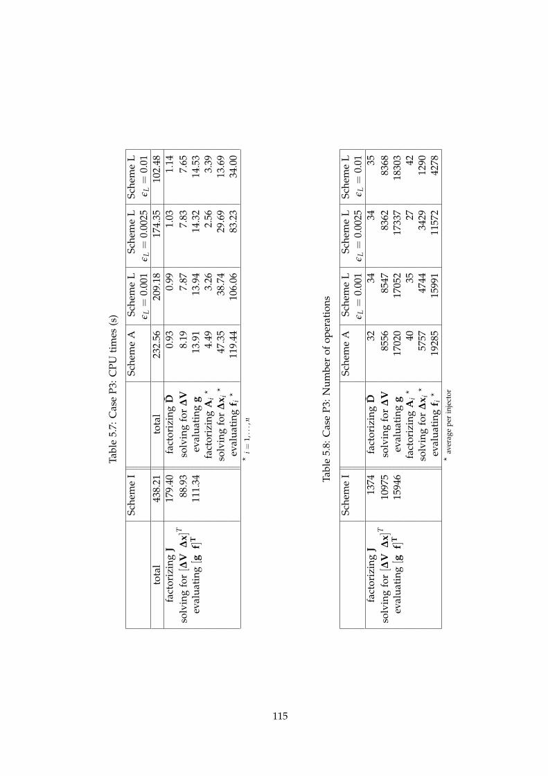
Tabl
e5.
7:C
ase
P3:C
PUti
mes
(s)
Sche
me
ISc
hem
eA
Sche
me
LSc
hem
eL
Sche
me
Lε L
=0.
001
ε L=
0.00
25ε L
=0.
01to
tal
438.
21to
tal
232.
5620
9.18
174.
3510
2.48
fact
oriz
ing
J17
9.40
fact
oriz
ing
D0.
930.
991.
031.
14so
lvin
gfo
r[∆
V∆
x]T
88.9
3so
lvin
gfo
r∆
V8.
197.
877.
837.
65ev
alua
ting
[gf]
T11
1.34
eval
uati
ngg
13.9
113
.94
14.3
214
.53
fact
oriz
ing
Ai?
4.49
3.26
2.56
3.39
solv
ing
for
∆x i
?47
.35
38.7
429
.69
13.6
9ev
alua
ting
f i?
119.
4410
6.06
83.2
334
.00
?i=
1,..
.,n
Tabl
e5.
8:C
ase
P3:N
umbe
rof
oper
atio
ns
Sche
me
ISc
hem
eA
Sche
me
LSc
hem
eL
Sche
me
Lε L
=0.
001
ε L=
0.00
25ε L
=0.
01fa
ctor
izin
gJ
1374
fact
oriz
ing
D32
3434
35so
lvin
gfo
r[∆
V∆
x]T
1097
5so
lvin
gfo
r∆
V85
5685
4783
6283
68ev
alua
ting
[gf]
T15
946
eval
uati
ngg
1702
017
052
1733
718
303
fact
oriz
ing
Ai?
4035
2742
solv
ing
for
∆x i
?57
5747
4434
2912
90ev
alua
ting
f i?
1928
515
991
1157
242
78?
aver
age
per
inje
ctor
115
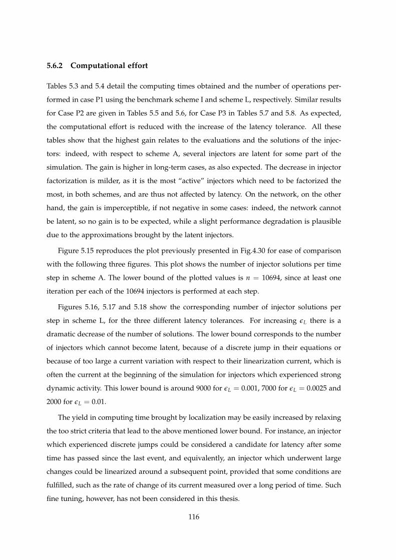
5.6.2 Computational effort
Tables 5.3 and 5.4 detail the computing times obtained and the number of operations per-
formed in case P1 using the benchmark scheme I and scheme L, respectively. Similar results
for Case P2 are given in Tables 5.5 and 5.6, for Case P3 in Tables 5.7 and 5.8. As expected,
the computational effort is reduced with the increase of the latency tolerance. All these
tables show that the highest gain relates to the evaluations and the solutions of the injec-
tors: indeed, with respect to scheme A, several injectors are latent for some part of the
simulation. The gain is higher in long-term cases, as also expected. The decrease in injector
factorization is milder, as it is the most “active” injectors which need to be factorized the
most, in both schemes, and are thus not affected by latency. On the network, on the other
hand, the gain is imperceptible, if not negative in some cases: indeed, the network cannot
be latent, so no gain is to be expected, while a slight performance degradation is plausible
due to the approximations brought by the latent injectors.
Figure 5.15 reproduces the plot previously presented in Fig.4.30 for ease of comparison
with the following three figures. This plot shows the number of injector solutions per time
step in scheme A. The lower bound of the plotted values is n = 10694, since at least one
iteration per each of the 10694 injectors is performed at each step.
Figures 5.16, 5.17 and 5.18 show the corresponding number of injector solutions per
step in scheme L, for the three different latency tolerances. For increasing εL there is a
dramatic decrease of the number of solutions. The lower bound corresponds to the number
of injectors which cannot become latent, because of a discrete jump in their equations or
because of too large a current variation with respect to their linearization current, which is
often the current at the beginning of the simulation for injectors which experienced strong
dynamic activity. This lower bound is around 9000 for εL = 0.001, 7000 for εL = 0.0025 and
2000 for εL = 0.01.
The yield in computing time brought by localization may be easily increased by relaxing
the too strict criteria that lead to the above mentioned lower bound. For instance, an injector
which experienced discrete jumps could be considered a candidate for latency after some
time has passed since the last event, and equivalently, an injector which underwent large
changes could be linearized around a subsequent point, provided that some conditions are
fulfilled, such as the rate of change of its current measured over a long period of time. Such
fine tuning, however, has not been considered in this thesis.
116

0
10000
20000
30000
40000
50000
50 100 150 200
nb. of in
jecto
r solu
tions
t (s)
scheme A
Figure 5.15: Case P3: number of injector solutions per step (scheme A)
0
10000
20000
30000
40000
50000
50 100 150 200
nb. of in
jecto
r solu
tions
t (s)
scheme L, epsilon_L=0.001
Figure 5.16: Case P3: number of injector solutions per step (scheme L, εL = 0.001)
117

0
10000
20000
30000
40000
50000
50 100 150 200
nb. of in
jecto
r solu
tions
t (s)
scheme L, epsilon_L=0.0025
Figure 5.17: Case P3: number of injector solutions per step (scheme L, εL = 0.0025)
0
10000
20000
30000
40000
50000
50 100 150 200
nb. of in
jecto
r solu
tions
t (s)
scheme L, epsilon_L=0.01
Figure 5.18: Case P3: number of injector solutions per step (scheme L, εL = 0.01)
118

5.7 Chapter conclusion
The most important contribution of this chapter is the localization applied to the decom-
position of the dishonest Newton method algorithm: it brings a speed-up ranging between
2 and 3, with respect to scheme A, and between 4 and 6, with respect to scheme I, on the
PEGASE test system. The speed-up on the Hydro-Quebec system is not so important, on
the other hand, due to the relatively smaller size of the system.
119


Chapter6
Relaxing accuracy in time
O wer weiß, was in der Zeiten Hintergrunde schlummert? 1
This chapter starts with a review of methods which have been used to solve the power
system dynamic problem with a varying level of accuracy: the principles of Quasi-Steady-
State method are also briefly described. The concept of time-averaging of the continuous
dynamics is introduced and the role of the discrete part of the model is analyzed in more
detail. Modelling and solving guidelines have been established and safeguards against
cycling between discrete states are considered. Relevant results on the three test systems
close this chapter showing that the computational effort of the proposed approach is greatly
reduced with respect to a detailed simulation, while the fast transients of the simulated
outputs can be gradually filtered out with the increase of the step size.
6.1 Temporal accuracy relaxation in literature
With temporal relaxation of accuracy we refer to the fact that some fast components of the
response may not be of interest, especially in long-term simulations, and could thus be
partially or totally omitted: this can be achieved through the use of a different solver or
through a simplification of the model.
1Oh who can see what sleeps in time, behind the face of things? Johann Christoph Friedrich von Schiller, in DonKarlos, Infant von Spanien. English translation by H. Collier Sy-Quia and P. Oswald in Don Carlos.
121

The complete omission of fast dynamics through model simplification is the heart of
the Quasi-Steady-State (QSS) approximation of long-term dynamics [VCJMP95]. In the
QSS approximation, Equations (2.4) are split into slow and fast components, ws and w f ,
respectively:
ws = ψds(y, w f , ws, z, V, I, ωre f ) (6.1)
w f = ψd f (y, w f , ws, z, V, I, ωre f ) (6.2)
The fast components are considered at equilibrium and Eq. (6.2) is replaced by
0 = ψd f (y, w f , ws, z, V, I, ωre f ) (6.3)
A more recent version of the QSS algorithm also considered frequency dynamics [GLVC05].
While the main advantage of the QSS approach is a speed-up of orders of magnitude with
respect to detailed simulation of the full model [VCM97], some drawbacks limit the scope
of this method:
• the separation of slow and fast components might not be possible for a complex black
box model. Automatic model simplification methods that can deal with realistic, hy-
brid power system models are yet to be developed. More on this problem will come
later in this section;
• the approach itself needs a different model than the one used for detailed simulation,
which requires additional overhead for creation, validation and maintenance. The
creation of a simplified model also requires a good knowledge of the process itself, so
it is not suitable for black box models;
• a long-term degradation of system operating conditions may result in motor stalling
or loss of synchronism [VCV08]. In this case, a fast instability of the full model (2.4)
appears as an early singularity of the QSS model (6.1,6.3) that gives little information
about the nature of the problem1;
• following a large disturbance, the system may become unstable in the short-term pe-
riod and, hence, even not enter the long-term period. Detecting this situation requires
to couple detailed and QSS simulations, as it will be seen in greater detail in Chapter 7;
1In practical applications [VCM97], however, such fast instabilities were found to take place at low voltages,where the system evolution was anyway unacceptable in the context of DSA.
122

• a more accurate simulation may require to retain some of the fast dynamics.
Another algorithm that relies on the time-scale separation of power system phenomena
to solve the different parts of the system with different levels of details (i.e. step sizes) is the
variable partitioning multi-rate method [CC08], which adapts the subdomains according to
the “level of activity” of the variables involved. It is our perception that the separation of
variables in different subsets might be cumbersome, if not impossible at all, for realistic
power system models. While in classical multi-rate methods the subdivision of differential
variables is decided beforehand, reference [CC08] proposes heuristics for the separation
of algebraic variables in between slow and fast subsets, a delicate operation insofar as an
algebraic dynamics is infinitely fast by definition, and the algebraic variables can only be
clustered based on their interaction with other variables.
In the author’s opinion, though, the main problem in the use of QSS or multi-rate
approaches lies in the subdivision of the differential variables themselves: in fact, while the
open-loop “time constant” of a process can be easily determined, it is the closed-loop one
which actually matters. And if the closed-loop includes the network, as it is often the case
in power systems studies, this computation is not practical, as it involves the elimination of
a large number of algebraic variables 1.
6.2 Time-averaging of continuous dynamics
In nonlinear dynamical systems theory, the procedure of replacing a vector field by its
average (over time or an angular variable) in order to obtain asymptotic approximations
to the original system is called averaging [SVM07]. In spite of the mathematical niceties of
this theory, its application to power system dynamics might be hindered by several factors:
(i) the averaging period is unknown in advance, (ii) the averaging period varies widely,
since the oscillations experienced in power systems belong to very different time-scales and
(iii) the physical meaning of averaging systems which exhibit hybrid continuous-discrete
behavior is not straightforward.
1In 2011, after a seminar given in Liege by a Control specialist, the author once raised the question onhow to discriminate between fast and slow variables in large differential-algebraic systems in a feasible way(usually the subsets are already given as input data in test problems). The answer was to eliminate the algebraicvariables. However, a practical way to eliminate algebraic variables on a system slightly larger than academictoy problems, is, in the author’s opinion, still to be found. The gist of this brief autobiographical argumentis that the problem of variable partitioning in black box models seems still to remain largely unsolved, evenoutside the power system community.
123

Nonetheless, the concept behind this mathematical theory, i.e. the possibility of getting
averaged trajectories, is highly appealing. The idea behind time-averaging is to perform time
simulation with L-stable methods using large enough steps so that some fast dynamics are
discarded while concentrating on the average evolution. In the general case, no theoretical
proof can be given that the obtained solution coincides with an averaged form of the original
trajectory. However, a good interpretation of the results obtained in practice is provided by
the following limit:
limh→∞
(−w(tj) + ∑o
`=1 γ` w(tj−`) + h β w(tj))
h= β w(tj) (6.4)
Equation (6.4) is the limit of the BDF (3.4), divided by h, for h→ ∞. After the algebraized
equations have been solved, the numerator in the left-hand side of (6.4) is brought to zero.
This means that at the limit the derivative w(tj) is zero, i.e. the simulated response of the
system is at equilibrium. A wider interpretation of this result is that the BDF formula tends
to the underlying system equilibrium as the step size is increased.
Conversely, non L-stable methods may produce spurious oscillations if they are used
with a step size significantly larger than the smallest time constant. Figure 6.1 shows a
simple example of application of respectively an L-stable (BEM) and a non L-stable (TM)
method to the test equation (3.7) with λ = 10, w(0) = 1, using a time step size h of
1 s, i.e. ten times larger than the time constant 0.1 s. The output computed with BEM
shows a consistent delay and reaches equilibrium quite soon. Conversely, TM returns an
unacceptable purely numerical oscillatory evolution.
The approach followed in this work consists of simulating the original, detailed model
with a solver that allows “filtering” out the fast dynamics by taking intentionally large steps.
The most significant advantage of this approach is that no simplification is performed of
the models, i.e. they are the same as in detailed simulation. Significant reductions of the
computational effort can be expected from the use of large steps, approximately given by
the ratio between the step size used in detailed simulation and the larger step used for
time-averaging.
The property of L-stable methods that allows integrating with steps significantly larger
than the smallest system time constants is known in numerical analysis [AP98, CK06]. The
use of BDF for their L-stable properties in power system dynamics can be traced back to
[ABJ94], while more recent uses are documented in [FVC09, WC11]. The method is also
124

-0.8
-0.6
-0.4
-0.2
0
0.2
0.4
0.6
0.8
1
0 2 4 6 8 10
w (
pu)
t (s)
reference L-stable solver (BEM)
non L-stable solver (TM)
Figure 6.1: Solutions of w = −10 w with different methods
used in a wide variety of other engineering problems, e.g. cloth dynamic simulation in
computer graphics [BW98].
On the other hand, the price to pay with L-stable methods is that they overdamp oscilla-
tions whose period is comparable to the step size. This undesired hyper-stability property
limits the step size used for detailed simulation. It suggests to use higher order BDF, since
the hyper-stability decreases with the order of the formula used. Unfortunately, BDF of
order larger than 2 do not exhibit the equally important property of A-stability.
Note the the hyper-stability property, which represent a limitation of the method for
detailed simulation of power system dynamics, has been used in electromagnetic transient
simulations as a feature to suppress the numerical oscillations arising from strong disconti-
nuities [ML89].
6.3 Handling of discrete dynamics
For a large class of continuous-time dynamics, in so far as accuracy can be somewhat re-
laxed, the step size of an L-stable method is limited only by the convergence of the Newton
iterations used to solve the algebraized equations [FVC09]. However, power system models
125

are also hybrid [HP00] and the proper handling of discrete events requires caution when
the time step is increased. To the author’s knowledge, this aspect has been relatively less
investigated in the literature; preliminary investigations were reported in [FCPVC11].
In the context of time-averaging, the following scheme is proposed for the ex post treat-
ment of discrete events:
1. at time t, starting from the state vector xt, take a step of length h. Let x(1)t+h be the
corresponding state vector;
2. at this time the jump conditions (2.13) are checked;
3. if it is detected that a state event has occurred in between t and t + h, z is changed
accordingly, and the step from t to t+ h is repeated with the flow (2.12) corresponding
to the new z, yielding the new value x(2)t+h of the state vector;
4. steps 2 and 3 are repeated, updating the state vector, until no jump occurs any longer
or a maximum number of jumps is reached. This yields the final state vector for the
current step;
5. then, the simulation proceeds with a new step.
Newton iterations are performed to pass from xt to x(j)t+h (j = 1, 2, . . .). It is essential
to iterate until reaching a solution x(j)t+h accurate for the current flow, before checking the
jump conditions (step 2). In other words, the flow must not be changed during the Newton
iterations, otherwise, incorrect and/or unpredictable jumps can be experienced.
Figure 6.2 shows a classical example of hybrid dynamics, namely an integrator with a
non-windup lower limit.
Let us define z as a discrete variable with value 1 if x < 3 and value 0 if x = 1. This
system is described by the following continuous-time equation of type (2.12):
z x = z (u− x) + (1− z) (x− 1)
At t = 0− the system is at equilibrium and x(0) = u(0−) = 3. At t = 0+, u(0+) = 0.
The trajectories computed with different methods are plotted in Fig. 6.2 with
• solid line: closed-form exponential solution x(t) = max(3e−t; 1);
• dotted line: BEM numerical solution computed with steps of 1 s and detailed handling
of state events;
126

t
x
1s
xu+ −
11
0 1 2
2
3
3
Figure 6.2: Integrator with non-windup limit, and example of response
• dashed line: BEM numerical solution computed with steps of 1 s and ex post handling
of state events as we propose.
The corresponding discrete event is taking place at t = ln(3) ' 1.1 s, in the closed-
form exponential solution. Let us stress that the closed-form solution is just provided as a
reference, but cannot practically be computed in even slightly more complex systems.
The most important effect of events on dynamic simulations is that they force the solver
to adjust the length of continuous-time evolution intervals in order to land over the event
times, as explained in Section 3.5. This mechanism, in case of many events, leads to a re-
duction of the average step size (and hence an increase in the number of steps). Moreover,
all (network and injector) Jacobians used in the Newton iterations have to be updated and
re-factorized when h changes significantly (the latter is involved in the algebraized differ-
ential equations). Coming back to the example in Fig. 6.2, with the detailed handling, the
state event should take place at 1.5 s: let us stress that this is dependent on the integration
formula and on the discretization interval. The detailed handling of discrete events is accu-
rate when the solution is performed with small integration steps. However, paradoxically,
the detailed handling is not as accurate as the name would suggest if comparatively large
steps are taken, as Fig. 6.2 shows: in fact, the delay in computing the switching time is due,
in this example, to the large truncation error committed because of the large steps used.
With the ex post treatment of discrete events, conversely, the event is not precisely located
in a specific instant, but it takes place in between the beginning and the end of a step, in
the case of Fig. 6.2 in between 1 and 2 s. The system equations are satisfied at the start and
final point of the step, and no attempt is made to identify the actual switching instant. It is
believed that for the envisaged application this constitutes an acceptable approximation.
127
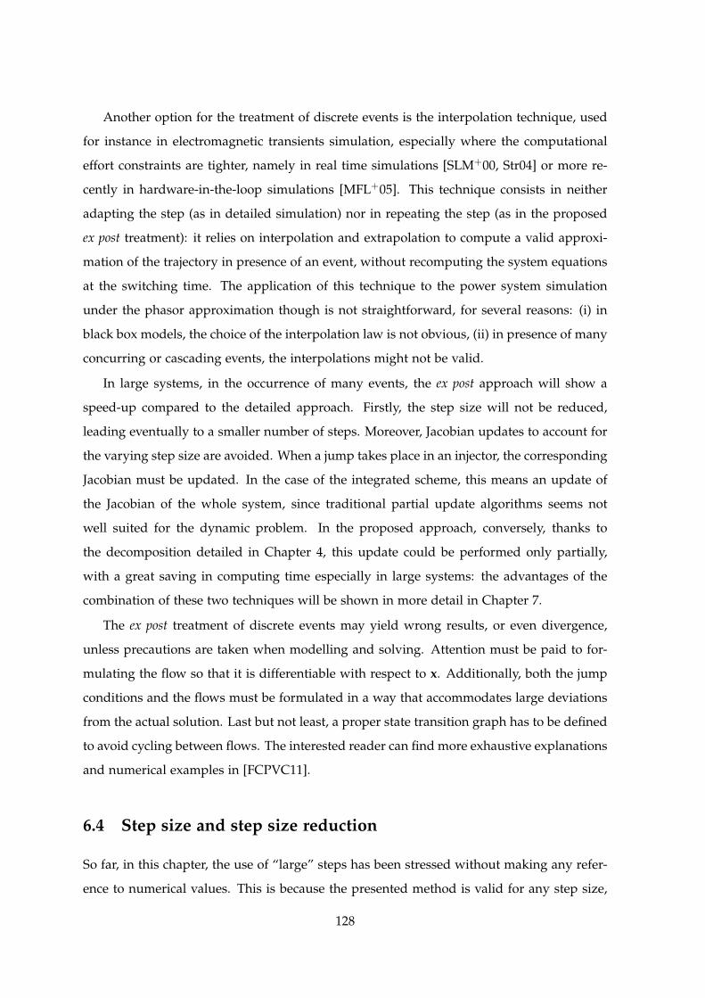
Another option for the treatment of discrete events is the interpolation technique, used
for instance in electromagnetic transients simulation, especially where the computational
effort constraints are tighter, namely in real time simulations [SLM+00, Str04] or more re-
cently in hardware-in-the-loop simulations [MFL+05]. This technique consists in neither
adapting the step (as in detailed simulation) nor in repeating the step (as in the proposed
ex post treatment): it relies on interpolation and extrapolation to compute a valid approxi-
mation of the trajectory in presence of an event, without recomputing the system equations
at the switching time. The application of this technique to the power system simulation
under the phasor approximation though is not straightforward, for several reasons: (i) in
black box models, the choice of the interpolation law is not obvious, (ii) in presence of many
concurring or cascading events, the interpolations might not be valid.
In large systems, in the occurrence of many events, the ex post approach will show a
speed-up compared to the detailed approach. Firstly, the step size will not be reduced,
leading eventually to a smaller number of steps. Moreover, Jacobian updates to account for
the varying step size are avoided. When a jump takes place in an injector, the corresponding
Jacobian must be updated. In the case of the integrated scheme, this means an update of
the Jacobian of the whole system, since traditional partial update algorithms seems not
well suited for the dynamic problem. In the proposed approach, conversely, thanks to
the decomposition detailed in Chapter 4, this update could be performed only partially,
with a great saving in computing time especially in large systems: the advantages of the
combination of these two techniques will be shown in more detail in Chapter 7.
The ex post treatment of discrete events may yield wrong results, or even divergence,
unless precautions are taken when modelling and solving. Attention must be paid to for-
mulating the flow so that it is differentiable with respect to x. Additionally, both the jump
conditions and the flows must be formulated in a way that accommodates large deviations
from the actual solution. Last but not least, a proper state transition graph has to be defined
to avoid cycling between flows. The interested reader can find more exhaustive explanations
and numerical examples in [FCPVC11].
6.4 Step size and step size reduction
So far, in this chapter, the use of “large” steps has been stressed without making any refer-
ence to numerical values. This is because the presented method is valid for any step size,
128

with the reservation, of course, that accuracy degrades with the increase of the step size.
It is thus possible to state that, in case of step size which are comparable to the smallest
time constant of the system, the proposed approach will perform as accurately as a detailed
simulation using steps of the same order of magnitude.
For instance, both BDF of order 2 and TM are second-order integration methods and
for the step size used in detailed simulation, their solution accuracy is comparable. On the
other hand, for increasing h, BDF cannot reproduce fast oscillations by the combined effects
of hyper-stability and limited resolution (supposing, for instance, that at least 4 points per
period are needed to describe a sinusoid, oscillations faster than 0.5 Hz are not reproduced
with steps larger than 0.5 s). Time-averaging enables the simulation to concentrate over
aperiodic changes and slow oscillations, while neglecting the fast ones.
Another reason for not taking too large step sizes has to do with the discrete dynamics
also present in the model. As discussed above, to preserve computational efficiency, the
exact jump instants are not identified: instead, they are accounted for at the next discrete
time. Hence, too large a step size would delay the transitions and artificially synchronize
multiple events.
Finally, larger step size generally means more Newton iterations per step. Hence, it may
be required to momentarily reduce the step size in case of divergence, e.g. when the system
undergoes a significant aperiodic change [FVC09].
The proposed approach consists in: (i) integrating with a maximum step h chosen in
accordance with the requirements above, (ii) reducing the step size automatically when
the Newton iterations exhibit convergence difficulties, and (iii) recovering to h as soon as
possible.
Note that this step size control differs from the traditional local-truncation-error based
control [Gea71]. Indeed, the latter criterion makes little sense in so far as accuracy require-
ments are relaxed and the emphasis is put on the coarse response of the system.
The logic to control the step size, when convergence difficulties are met, consists of
bounding the computational effort estimated as the number of Newton iterations. The step
size is first reduced by an arbitrary factor: hnew = h/k. If good convergence is regained, the
simulation proceeds with another step; otherwise successive reductions are applied until
reaching the minimum step size (in case of failure at the minimum step size divergence is
declared and the simulation stops). In our tests k = 2 was found to work satisfactorily.
Subsequent steps are taken following a logic of estimation of the step computational
129

effort, supposed to grow with the step size. Namely, the effort is estimated by the number n
of Newton iterations performed in order to solve the last time step. The step size is chosen
in order to match a desired number of iterations N. A “dead-band” M on the effort is
considered in order to avoid too frequent step size variations.
More precisely, the step size is varied as follows, depending on the observed value of n:
hnew =
h
Nn + M
if n < N −M
h if N −M ≤ n ≤ N + M
hN
n−Mif N + M < n
(6.5)
the purpose being to come back as quickly as possible to the default step chosen. When
the default step size value is reached, the fixed step size strategy is resumed. The choice of
parameters k, N and M may be system dependent and usually results from of a trial-and-
error procedure. In the present implementation N = 5 and M = 2.
In an earlier publication [FVC09] the mismatch vector of the first Newton iteration was
suggested as a measure of computational effort but experience has shown that it is impracti-
cal for two reasons: (i) in case of large systems it would require a significant computational
overhead and (ii) the mismatch vector value cannot be interpreted easily in black box mod-
els, especially for the algebraic part of the model.
The hybrid behavior of power systems can give rise to another numerical difficulty,
especially when overstepping an event with a large step. The problem most likely to remain
unsolved, even after adjusting the flow equations and/or the jump conditions, is the cycling
between flows: this phenomenon happens when a discrete state cannot be determined after
a step and this step is repeatedly computed while the system keeps passing through two or
more discrete states without settling in any.
In order the simulation to proceed, a first option consists in leaving the time step with
the last available solution x(j), once the number of flow jumps reaches a maximum, and pro-
ceeding with the next step. We found in many cases that the problem disappears at the next
time step. This temporary discrepancy may be acceptable for the envisaged applications.
However, there is no guarantee that the problem will disappear.
In so far as the problem stems from severely overstepped events, another option is to
reduce the step size h until the problem is no longer met. h is first reduced by a factor
k: hnew = h/k (our simulations have shown that k = 2 is a convenient choice). If no event
cycling takes place any longer, the step is accepted; otherwise further reductions are applied
130

timer
gain reductiontransient
exciter
32
4
y ≥ 01s y < 0
y
1 L2
0
10
−1
−0.1 0
r
−1
f
L11s
i f d
ilimf d
+
−
min
V+
−
Vo
G(1 + sTa)
1 + sTbv f d
−
+y1 y2
Figure 6.3: Block diagram of voltage regulator, field current limiter and exciter
until the problem is solved. Then, the original step size h is restored and the simulation
proceeds. The application of this strategy to a power system example is detailed in the next
section.
6.5 Example of cycling between flows
The example has been obtained with on the Nordic32 system Case N3 (see Section 4.6).
At t = 1 s, the transmission line 4032 − 4044 is tripped. This causes the neighbouring
voltage-controlled generator g14 to operate above its permanent field current limit. The
block-diagram of the voltage regulator, field current limiter and exciter is shown in Fig. 6.3.
In normal operating conditions the field current i f d is much lower than its permanent
limit ilimf d and the output of block 1 is −1. This keeps the integrator of block 2 at its lower
limit L1, which is negative. It results that the switch in block 3 remains in the lower position
and passes the input Vo −V. The minimum gate receives two equal inputs, and we assume
it selects y1, the output of block 3.
When the machine operates with i f d > ilimf d , the output y of the integrator block 2 grows,
until it reaches a positive value, causing block 3 to switch. Thus, block 2 acts as a timer
and provides inverse-time characteristic to the OEL. After block 3 has switched, the inputs
of the minimum gate are Vo − V > 0 and y1 = ilimf d − i f d < 0, respectively. Hence, the gate
keeps on selecting y1.
The purpose of this minimum gate is to reset the machine under voltage control when-
ever operating conditions improve to the point that Vo −V becomes negative. However, in
131

a
b
3.15
ilimf d
3.00
−0.2
−0.3
−0.4
−0.1
050.049.5
50.049.5
yi f d
t
t
3.30
Figure 6.4: Detailed view of iterations when the OEL becomes active
the following example, no such reset takes place and the minimum gate selects its w input
throughout the whole simulation.
After the line outage, i f d starts increasing and becomes larger than ilimf d at t = 1.5 s. The
step from t = 1 to t = 1.5 is thus repeated to account for the jump from flow f = 0 to flow
f = i f d − ilimf d in block 1. The output of block 1 becomes positive, causing a jump in block 2,
corresponding to y leaving its lower limit L1.
Variable y keeps on increasing until it becomes positive, causing the switch in block 3 to
change, i.e. the machine to switch from voltage to field current control in between t = 49.5
and t = 50. A zoom on the evolution of i f d and y is given in Fig. 6.4.
Here is a detailed analysis of this step:
• at the beginning of the step, y < 0, block 3 is selecting its input Vo − V; the step
converges to a positive y value at t = 50, triggering a jump in block 3. This is shown
with dotted lines in Fig. 6.4;
• the step is restarted with block 3 passing ilimf d − i f d. However, when passing through
the exciter and the synchronous machine this signal has such a pronounced effect on
the system that a value i f d close to ilimf d is retrofitted to the OEL, which causes the
updated value of y at t = 50 to get back to negative value. This is shown with dashed
lines in Fig. 6.4. However, this triggers the reverse jump of block 3, and causes the
jump handling procedure to endlessly oscillate between voltage and field control.
The variable y that controls block 3, when integrated with “large” derivative i f d − ilimf d = a
132

(see Fig.6.4) triggers the jump to the flow with “small” derivative i f d− ilimf d = b, where b < a
due to the above mentioned fast retroaction. Conversely, when integrated with the “small”
derivative b, it triggers the jump to the flow with “large” derivative a.
As indicated in Section 6.4, two options are available to proceed with the simulation: (i)
break the cycle and accept the last available solution, or (ii) reduce the step to have more
chances to avoid cycling. The first option yields satisfactory convergence but delays the
OEL action by one step. The result of second option is shown with solid line in Fig. 6.4.
The step size has been halved after meeting the problem at t = 49.5. The simulation passes
from t = 49.50 to t = 49.75 without jump. Then the machine correctly switches under field
limit in between t = 49.75 and t = 50.00. At 49.75 s, the value y escapes the region of
non-existence of solutions and can thus converge successfully.
6.6 Time-averaging results on Nordic32 system
This section shows applications of time-averaging on Cases N1, N2, N3 and N4, respectively
(see Section 4.6). Case N5 is not considered here since it involves a short circuit that cannot
be simulated with the large steps considered in this chapter. The outputs have been obtained
with a time-averaged dishonest Newton scheme (denoted “T” in the plots). More details
about this and the other solvers are given in Appendix A.5. Table 6.1 summarizes the
DTW distances between the outputs of scheme T and I (the latter being the reference). It
should be stressed right away that δ and σ are significantly higher than µ in most of the
cases, confirming that time-averaging renders the average system evolution, thus keeping µ
relatively small. Relevant results concerning the speed-up are detailed in the next sections,
on the larger systems.
6.6.1 Case N1
Figure 6.5 shows a zoom of the active power flow in the other circuit of line 1013-1014.
The long-term evolutions given by the T and the I schemes then become indistinguishable.
As expected, increasing of the step size h smooths the oscillations, up to the limit case of
h = 0.5 s that nearly reaches the underlying equilibrium in one step.
133

120
140
160
180
200
220
0 1 2 3 4 5
active p
ow
er
(MW
)
t (s)
scheme I scheme T, h=0.1 scheme T, h=0.2 scheme T, h=0.5
Figure 6.5: Case N1: active power flow in one circuit of line 1013-1014
2.66
2.68
2.7
2.72
2.74
2.76
2.78
2.8
2.82
2.84
0 5 10 15 20
field
voltage (
pu)
t (s)
scheme I scheme T, h=0.1 scheme T, h=0.2 scheme T, h=0.5
Figure 6.6: Case N2: field voltage of generator g15
134

6.6.2 Case N2
Case N2 is another scenario where the smoothing effect of time-averaging is highlighted. A
zoom on the field voltage evolution of generator g15 is provided in Fig. 6.6. As expected,
the time-averaging effect is increased with the step size. The long-term evolution is not very
different from the one shown in Fig. 4.10.
6.6.3 Case N3
Case N3 allows to test time-averaging on a collapse scenario. The voltage at bus 1041,
evolving towards collapse, is plotted in Fig. 6.7. While the overall aperiodic behavior is
tracked, smaller oscillations are filtered out. The evolutions show some differences towards
the end of the simulation, but it is important to observe that the transmission voltage is
already quite low, and the fate of the system already inevitable!
Figure 6.8 depicts the speed deviation of generator g6. The loss of synchronism is
detected some seconds in advance by the time-averaged simulations with respect to the
benchmark; this does not mean, however, that time-averaging generally tends to anticipate
events with respect to detailed simulation: delays have been also experienced.
The outputs are computed with the indicated steps up to the end of the simulation,
since the Newton convergence is satisfactory and no step size reduction is required, which
is quite noticeable!
6.6.4 Case N4
Case N4 underlines the weak point of stiff-decay methods, when the step size is not limited.
Figures 6.9 and 6.10 show the field voltage and speed deviation of generator g17.
Let us recall that this simulation is purely an academic exercise, since the power system
stabilizers of the system are disabled in order to obtain an oscillatory evolution. One may
argue that this can happen when the system undergoes a progressive degradation such
that the operative point becomes oscillatory unstable, for instance under the effect of OELs
by-passing the stabilizers [VCV08], or due to cascade line trippings.
In the test of Figs. 6.9 and 6.10, however, the variety of the chosen step sizes allow us
to appreciate the influence of hyper-stability. With steps of 0.1 s, the loss of synchronism
is detected two rotor oscillations later. Integrating with steps of 0.2 s, returns a case of
135

0.7
0.75
0.8
0.85
0.9
0.95
1
1.05
0 20 40 60 80 100 120 140 160 180
voltage m
agnitude (
pu)
t (s)
scheme I scheme T, h=0.1 scheme T, h=0.2 scheme T, h=0.5
Figure 6.7: Case N3: voltage at transmission bus 1041
0
0.002
0.004
0.006
0.008
0.01
0.012
0 20 40 60 80 100 120 140 160 180
speed d
evia
tion (
pu)
t (s)
scheme I scheme T, h=0.1 scheme T, h=0.2 scheme T, h=0.5
Figure 6.8: Case N3: synchronous machine speed of generator g6
136

1
2
3
4
5
6
0 5 10 15 20 25
field
voltage (
pu)
t (s)
scheme I scheme T, h=0.1 scheme T, h=0.2 scheme T, h=0.5
Figure 6.9: Case N4: field voltage of generator g17
-0.01
0
0.01
0.02
0.03
0.04
0.05
0.06
0.07
0 5 10 15 20 25
speed d
evia
tion (
pu)
t (s)
scheme I scheme T, h=0.1 scheme T, h=0.2 scheme T, h=0.5
Figure 6.10: Case N4: synchronous machine speed of generator g17
137

marginal instability, which could still be flagged as dangerous 1. A step of 0.5 s, conversely,
completely overlooks the instability and returns a stable trajectory. In Chapter 7, we will
show that simulating for a short period with “small steps” can mitigate the hyper-stability
problem.
Table 6.1: DTW distances
Fig. h δ µ σ Unit0.1 1.5244 0.0578 1.5247 MW
6.5 0.2 1.8562 -0.0856 1.8560 MW0.5 2.6842 -0.0467 2.6864 MW0.1 0.0001 0.0000 0.0001 pu
4.8 0.2 0.0003 -0.0000 0.0003 pu0.5 0.0006 -0.0000 0.0006 pu0.1 0.0017 -0.0000 0.0017 pu
4.9 0.2 0.0008 -0.0000 0.0008 pu0.5 0.0013 0.0000 0.0013 pu0.1 0.0001 0.0000 0.0001 pu
6.6 0.2 0.0049 -0.0001 0.0049 pu0.5 0.0087 -0.0003 0.0086 pu0.1 1.6896 -0.0499 1.6893 MW
4.11 0.2 2.9135 -0.0497 2.9139 MW0.5 5.5272 -0.0406 5.5287 MW0.1 0.0015 0.0001 0.0015 pu
6.7 0.2 0.0021 0.0002 0.0021 pu0.5 0.0032 0.0003 0.0032 pu0.1 0.0001 0.0000 0.0001 pu
6.8 0.2 0.0002 0.0000 0.0002 pu0.5 0.0002 0.0000 0.0002 pu0.1 0.1297 0.0205 0.1282 pu
6.9 0.2 0.4631 -0.0794 0.4567 pu0.5 0.6161 -0.1385 0.6010 pu0.1 0.0007 0.0002 0.0007 pu
6.10 0.2 0.0018 -0.0005 0.0017 pu0.5 0.0030 -0.0009 0.0029 pu
1Upon detection of such a situation, the simulation could be rerun with smaller steps or an eigenvalueanalysis could be carried out to eliminate any ambiguity.
138

6.7 Time-averaging results on Hydro-Quebec system
This section shows applications of time-averaging on Cases Q2, Q3 and Q4, respectively
(see Section 4.7). Time-averaging cannot be applied to Cases Q1 and Q5 since they simulate
a short circuit which is not compatible with the large steps used. The outputs have been
obtained with a time-averaged dishonest Newton scheme (denoted “T” in the plots). More
details about this and the other solvers are given in Appendix A.5. Since it is known that
the system is prone to instability, time-averaging has been limited to steps of 0.2 s.
6.7.1 Case Q2
Figure 6.11 shows the speed deviation of the COI. A good match can be observed between
the output of scheme T and the benchmark.
6.7.2 Case Q3
Case Q3 is interesting owing to the differences in MAIS activation. Figure 6.12 shows
a zoom of the voltage evolution at bus 709 with the indication of the switching voltage
threshold. The MAIS device switches off the reactor if the voltage stays below the threshold
for 1 s consecutively. In the output computed with scheme I, the voltage of bus 709 stays
below the threshold for slightly less than one second, thus no reactor is manoeuvered, while
with scheme A it stays just slightly longer, so that it triggers this large impact control.
Figure 6.13 provides the speed deviations of the COI, which settle to different values
due to one reactor unduly tripped. This case is slightly too severe to use time-averaging
over the whole simulation: the method presented in Chapter 7 is to be preferred.
6.7.3 Case Q4
A similar behavior happens in Case Q4 where the switching delay of the first MAIS, in
bus 715, triggers different sequences of reactor trippings, leading to some differences in the
system trajectory.
The variable of interest for this case is the voltage at transmission bus 702, provided in
Fig. 6.14. The overall match is acceptable for the reasons given in Section 4.7.4. Note that
the computed trajectories are indistinguishable up to the first reactor tripping.
139

-0.007
-0.006
-0.005
-0.004
-0.003
-0.002
-0.001
0
0 20 40 60 80 100
speed d
evia
tion (
pu)
t (s)
scheme I scheme T
Figure 6.11: Case Q2: deviation of COI speed
0.91
0.92
0.93
0.94
0.95
0.96
0.97
0.98
0.99
1
0 1 2 3 4 5
voltage m
agnitude (
pu)
t (s)
scheme I scheme T
MAIS switching threshold
Figure 6.12: Case Q3: zoom of the voltage evolution at transmission bus 709
140

-0.016
-0.014
-0.012
-0.01
-0.008
-0.006
-0.004
-0.002
0
0 20 40 60 80 100
speed d
evia
tion (
pu)
t (s)
scheme I scheme T
Figure 6.13: Case Q3: deviation of COI speed
0.95
0.955
0.96
0.965
0.97
0.975
0.98
0.985
0.99
0.995
1
0 50 100 150 200 250 300
voltage m
agnitude (
pu)
t (s)
scheme I scheme T
Figure 6.14: Case Q4: voltage at transmission bus 702
141
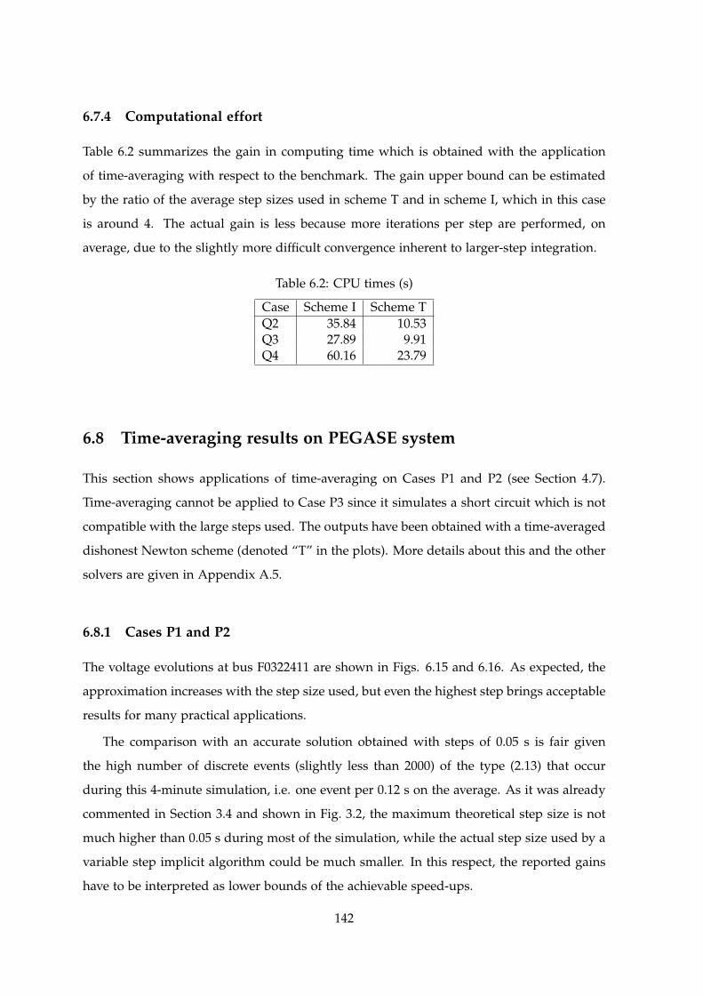
6.7.4 Computational effort
Table 6.2 summarizes the gain in computing time which is obtained with the application
of time-averaging with respect to the benchmark. The gain upper bound can be estimated
by the ratio of the average step sizes used in scheme T and in scheme I, which in this case
is around 4. The actual gain is less because more iterations per step are performed, on
average, due to the slightly more difficult convergence inherent to larger-step integration.
Table 6.2: CPU times (s)
Case Scheme I Scheme TQ2 35.84 10.53Q3 27.89 9.91Q4 60.16 23.79
6.8 Time-averaging results on PEGASE system
This section shows applications of time-averaging on Cases P1 and P2 (see Section 4.7).
Time-averaging cannot be applied to Case P3 since it simulates a short circuit which is not
compatible with the large steps used. The outputs have been obtained with a time-averaged
dishonest Newton scheme (denoted “T” in the plots). More details about this and the other
solvers are given in Appendix A.5.
6.8.1 Cases P1 and P2
The voltage evolutions at bus F0322411 are shown in Figs. 6.15 and 6.16. As expected, the
approximation increases with the step size used, but even the highest step brings acceptable
results for many practical applications.
The comparison with an accurate solution obtained with steps of 0.05 s is fair given
the high number of discrete events (slightly less than 2000) of the type (2.13) that occur
during this 4-minute simulation, i.e. one event per 0.12 s on the average. As it was already
commented in Section 3.4 and shown in Fig. 3.2, the maximum theoretical step size is not
much higher than 0.05 s during most of the simulation, while the actual step size used by a
variable step implicit algorithm could be much smaller. In this respect, the reported gains
have to be interpreted as lower bounds of the achievable speed-ups.
142

0.98
0.99
1
1.01
1.02
1.03
1.04
1.05
0 5 10 15 20
voltage m
agnitude (
pu)
t (s)
scheme I scheme T, h=0.2 scheme T, h=0.5 scheme T, h=1.0
Figure 6.15: Case P1: voltage at transmission bus F0322411
0.99
1
1.01
1.02
1.03
1.04
1.05
0 50 100 150 200
voltage m
agnitude (
pu)
t (s)
scheme I scheme T, h=0.2 scheme T, h=0.5 scheme T, h=1.0
Figure 6.16: Case P2: voltage at transmission bus F0322411
143
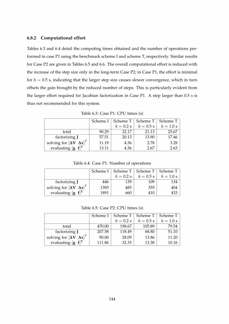
6.8.2 Computational effort
Tables 6.3 and 6.4 detail the computing times obtained and the number of operations per-
formed in case P1 using the benchmark scheme I and scheme T, respectively. Similar results
for Case P2 are given in Tables 6.5 and 6.6. The overall computational effort is reduced with
the increase of the step size only in the long-term Case P2; in Case P1, the effort is minimal
for h = 0.5 s, indicating that the larger step size causes slower convergence, which in turn
offsets the gain brought by the reduced number of steps. This is particularly evident from
the larger effort required for Jacobian factorization in Case P1. A step larger than 0.5 s is
thus not recommended for this system.
Table 6.3: Case P1: CPU times (s)
Scheme I Scheme T Scheme T Scheme Th = 0.2 s h = 0.5 s h = 1.0 s
total 90.29 32.17 21.13 25.67factorizing J 57.51 20.13 13.90 17.46
solving for [∆V ∆x]T 11.19 4.36 2.78 3.28evaluating [g f]T 13.11 4.36 2.67 2.63
Table 6.4: Case P1: Number of operations
Scheme I Scheme T Scheme T Scheme Th = 0.2 s h = 0.5 s h = 1.0 s
factorizing J 446 139 109 134solving for [∆V ∆x]T 1393 485 355 404
evaluating [g f]T 1891 660 410 433
Table 6.5: Case P2: CPU times (s)
Scheme I Scheme T Scheme T Scheme Th = 0.2 s h = 0.5 s h = 1.0 s
total 470.00 198.67 105.89 79.54factorizing J 207.58 118.49 68.80 51.10
solving for [∆V ∆x]T 90.00 28.09 13.86 11.20evaluating [g f]T 111.86 32.33 13.38 10.16
144
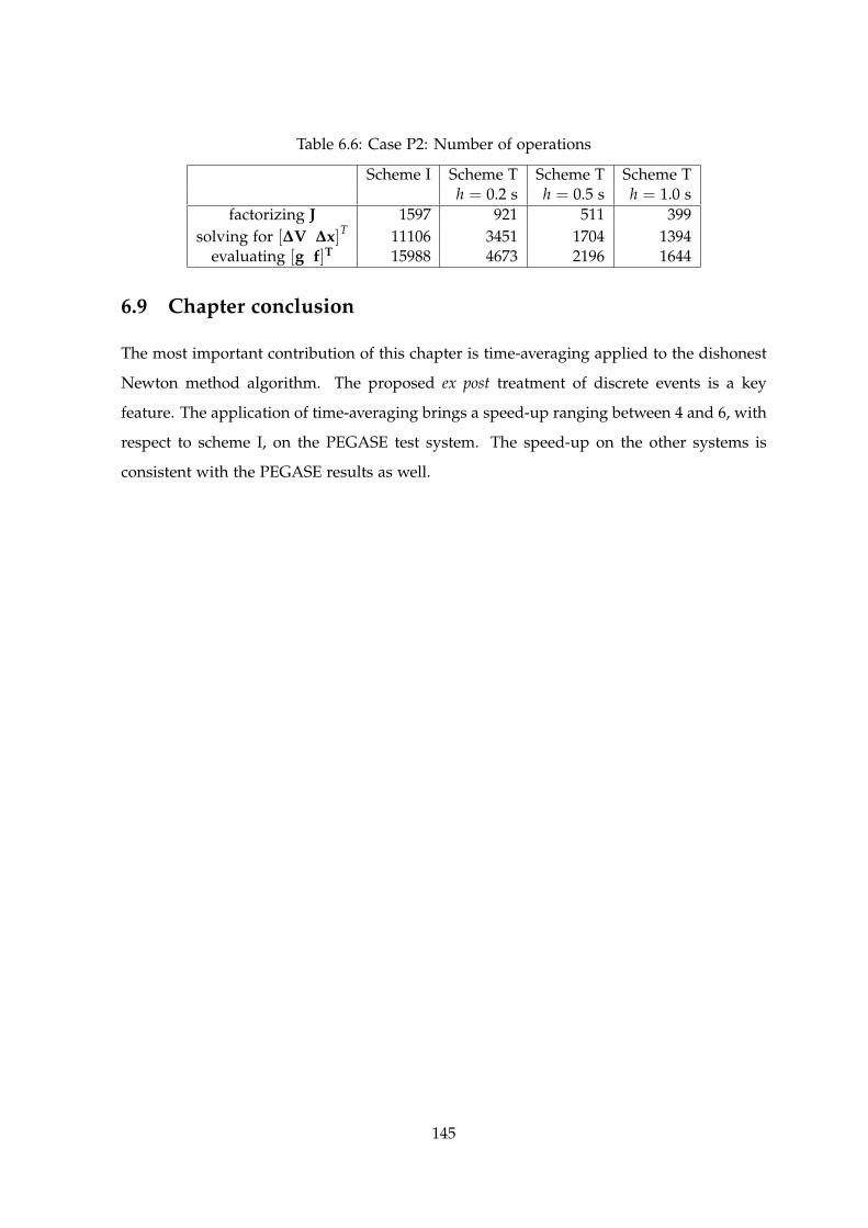
Table 6.6: Case P2: Number of operations
Scheme I Scheme T Scheme T Scheme Th = 0.2 s h = 0.5 s h = 1.0 s
factorizing J 1597 921 511 399solving for [∆V ∆x]T 11106 3451 1704 1394
evaluating [g f]T 15988 4673 2196 1644
6.9 Chapter conclusion
The most important contribution of this chapter is time-averaging applied to the dishonest
Newton method algorithm. The proposed ex post treatment of discrete events is a key
feature. The application of time-averaging brings a speed-up ranging between 4 and 6, with
respect to scheme I, on the PEGASE test system. The speed-up on the other systems is
consistent with the PEGASE results as well.
145


Chapter7
Combining detailed simulation with
accuracy relaxation techniques
Truth is much too complicated
to allow anything but approximations 1
This chapter delivers our final proposal on how to achieve a good compromise between
accuracy and efficiency of power system dynamic simulations. A general discussion on ac-
curacy of both modelling and simulation opens this chapter. Several approaches to combine
short-term detailed simulation with long-term simplified simulation are reviewed. An im-
portant aspect of this combination is the criterion to switch between short- and long-term
simulation: a universal criterion is not sought here, as the author believes that a combi-
nation of numerical experience and system knowledge can better inspire the heuristics for
such decision. The chosen heuristic criteria are described and relevant results for the three
test systems close this chapter showing that acceptable outputs can be obtained by com-
bining detailed simulation with the accuracy relaxation techniques presented in Chapters 5
and 6.
1John von Neumann, ne Neumann Janos Lajos, excerpt taken from The Mathematician, appeared in TheWorks of the Mind.
147

7.1 How accurate is a detailed simulation?
Before going further in this chapter, this section reviews the concepts of detailed and sim-
plified simulation that were used throughout this work: until Chapter 4, it was assumed
that a “detailed simulation” is the solution of Equations (2.1-2.5) discretized with a small
enough step size, with detailed handling of events and proper solution of discontinuities.
Now the question is: how accurate is a detailed simulation?
In fact, this question is crucial for the correct interpretation of simulation results. And
the answer is: a detailed simulation is not as accurate as its name might suggest.
It is convenient to split the question in two parts: model accuracy and solver accuracy.
Concerning the model, several reasons suggest that the absolute accuracy of a power system
simulation is kind of a myth:
• equations (2.1-2.5) represent the system under a few approximations (single phase
representation of an assumed balanced three-phase system, quasi-sinusoidal approxi-
mation, load aggregation or equivalencing, assumed load pattern, assumed intermit-
tent generation output, equivalencing of external networks, etc.) which might indeed
deliver a response which has some significant differences with respect to the real sys-
tem trajectory;
• the models and the parameters behind equations (2.1-2.5) are somewhat uncertain
or are anyway the result of model identification procedures which might not be ex-
tremely accurate for any operation mode, especially when the system conditions are
degraded.
In view of the elements above, it is clear that the detailed solution might indeed be
numerically accurate, but with respect to a model which is itself not fully accurate. The
overall simulation, even if it is performed with as much numerical accuracy as possible,
might give the illusion of accuracy, since it will not be fully accurate with respect to the
real, somewhat unknown, underlying process.
Seen from this perspective, it would be possible to relax some of the solver accuracy
constraints in favour of a faster simulation, especially when the obtained loss of accuracy
is comparable with the accuracy limitations of the model. The techniques described in
Chapter 5 and 6, if carefully applied, can indeed preserve the overall accuracy, using a
148

small enough latency tolerance and a small enough time step size where needed, while
providing a substantial speed-up.
7.2 Combination of short- and long-term simulations
When a power system is subject to a large disturbance (typically a fault), its dynamic re-
sponse can be decomposed into a short-term and a long-term period (if the system does not
lose stability in the short-term period, in which case it will not enter long-term, obviously).
The first few seconds of simulation, which are dominated by electromechanical oscillations,
belong to the short-term period, while thermal and voltage restoration processes are classi-
fied long-term and act in a time span ranging from around ten seconds to a few minutes.
It should be kept in mind though, that this division is a rough simplification since there is
no clear-cut boundary between short- and long-term. Also, in some cases, long-term events
may trigger phenomena in the short term, whose time scale is in the order of seconds: this
takes place for instance in Cases N3 and N5 (see Sections 4.6.3 and 4.6.5), where a field
current limited generator eventually loses synchronism.
In the simplest case, the long-term evolution is determined more by the topology change
resulting from clearing the fault than by the initial “impulse” given by the initiating short
circuit.
This simple case is also dealt with by the post-contingency power flow computation (of
the kind used for static security assessment), which aims at determining the final steady-
state, assuming that the system survived the short-term period and is stable in the long-
term. Post-contingency power flows suffer from two limitations: (i) the computation may
diverge for purely numerical reasons, and (ii) if the system has no long-term equilibrium
(this is the case in particular for long-term voltage instability), there is no solution, the
computation diverges and leaves the user without information.
There is, however, an additional limitation of power flow computation: the presence
of post-disturbance automatic controls (such as the MAIS devices in the Hydro-Quebec
system). Under the pressure of the electricity market, there is a trend to operate the system
with less (expensive) preventive security margins and to rely to a greater extent on post-
disturbance, corrective controls to stabilize the system and bring it within desired operating
limits. The identification of those control actions requires simulating the trajectory followed
by the system. This is why we advocate the use of dynamic simulation instead of power
149

flow computations for security assessment purposes.
In “mild” cases however, where the system is assumed to be short-term stable and its
long-term evolution is basically determined by the topological change resulting from the
fault clearing, it is possible to use some of the techniques mentioned in Chapter 6 over the
whole simulation period. Of course, in this case, the initiating fault is not simulated, only
the topological change that results from its clearing is considered.
However, this simplified handling may be inappropriate in three cases:
• the system is prone to short-term (angle or voltage) instability, which requires to check
its response to the initiating fault;
• the fault triggers some fast controls that help stabilizing the system. As already men-
tioned, the identification of those controls requires simulating the system evolution;
• that fault triggers some protections that disconnect some equipment (for instance trip-
ping of induction motors stalled under the effect of a fault lasting too long, discon-
nection of power electronics due to abnormal voltages, etc.).
Note that in the last two cases, the system enters the long-term period non only with
the topological change resulting from fault clearing but also with the changes from the
fast controls and/or the protections. To deal with those cases, it is appropriate to combine
detailed and simplified simulations, as follows:
• check the short-term period with detailed simulation;
• switch to simplified simulation for the long-term period.
In [KOO+93], a scheme is proposed that allows to switch between three simulation
modes:
• Transient stability simulation, using a fixed-time-step explicit integration formula;
• Extended-time simulation, using a variable-time-step implicit integration formula;
• QSS simulation.
The switching conditions are based on error estimation and frequency deviation. The
QSS mode requires the development and maintenance of a separate model, and brings
150
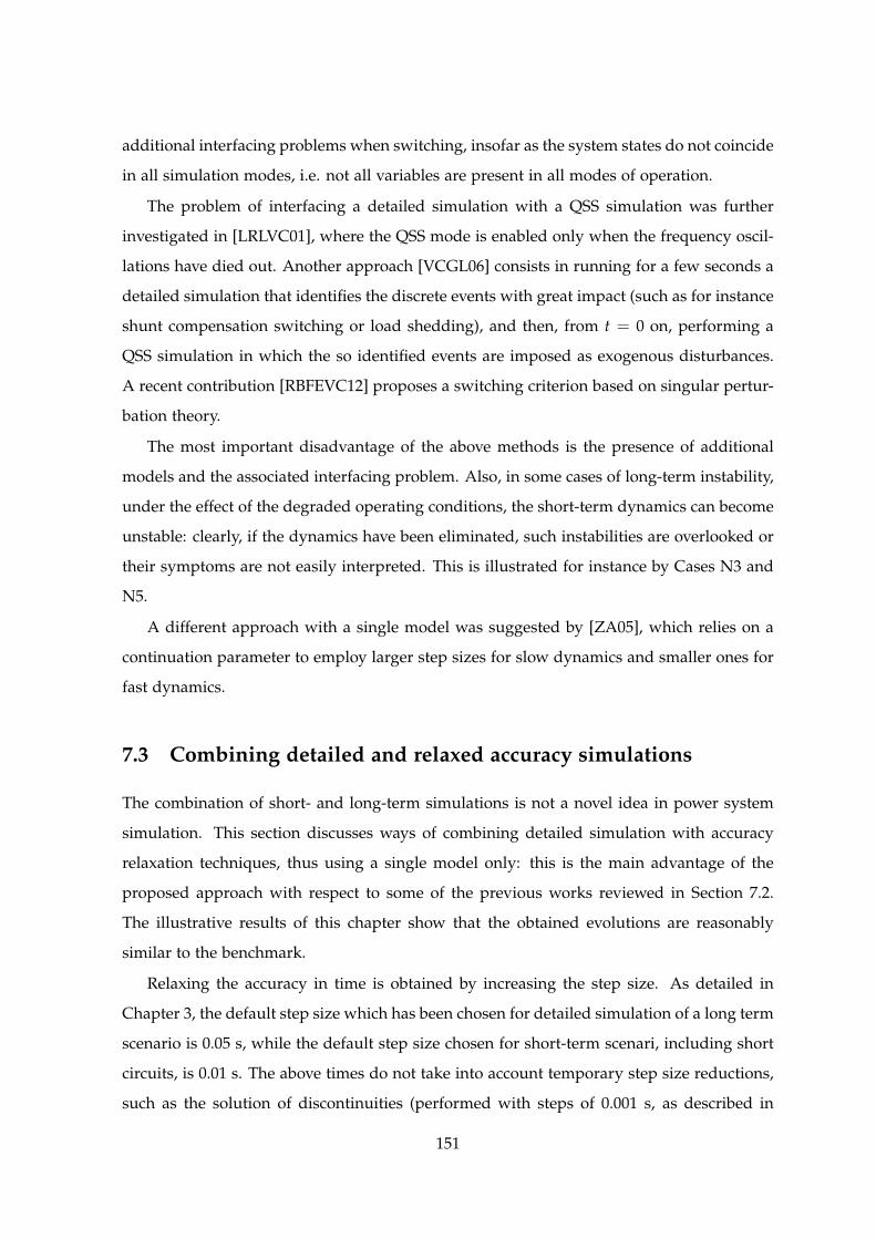
additional interfacing problems when switching, insofar as the system states do not coincide
in all simulation modes, i.e. not all variables are present in all modes of operation.
The problem of interfacing a detailed simulation with a QSS simulation was further
investigated in [LRLVC01], where the QSS mode is enabled only when the frequency oscil-
lations have died out. Another approach [VCGL06] consists in running for a few seconds a
detailed simulation that identifies the discrete events with great impact (such as for instance
shunt compensation switching or load shedding), and then, from t = 0 on, performing a
QSS simulation in which the so identified events are imposed as exogenous disturbances.
A recent contribution [RBFEVC12] proposes a switching criterion based on singular pertur-
bation theory.
The most important disadvantage of the above methods is the presence of additional
models and the associated interfacing problem. Also, in some cases of long-term instability,
under the effect of the degraded operating conditions, the short-term dynamics can become
unstable: clearly, if the dynamics have been eliminated, such instabilities are overlooked or
their symptoms are not easily interpreted. This is illustrated for instance by Cases N3 and
N5.
A different approach with a single model was suggested by [ZA05], which relies on a
continuation parameter to employ larger step sizes for slow dynamics and smaller ones for
fast dynamics.
7.3 Combining detailed and relaxed accuracy simulations
The combination of short- and long-term simulations is not a novel idea in power system
simulation. This section discusses ways of combining detailed simulation with accuracy
relaxation techniques, thus using a single model only: this is the main advantage of the
proposed approach with respect to some of the previous works reviewed in Section 7.2.
The illustrative results of this chapter show that the obtained evolutions are reasonably
similar to the benchmark.
Relaxing the accuracy in time is obtained by increasing the step size. As detailed in
Chapter 3, the default step size which has been chosen for detailed simulation of a long term
scenario is 0.05 s, while the default step size chosen for short-term scenari, including short
circuits, is 0.01 s. The above times do not take into account temporary step size reductions,
such as the solution of discontinuities (performed with steps of 0.001 s, as described in
151

Section 3.5), and the solution of non-converged or flow cycling case, as detailed in Section
6.4. In Chapter 6, conversely, time-averaging was obtained by imposing steps of 0.2, 0.5 or
1 s for the solution of long-term cases. The combined simulation will be performed on both
short- and long-term cases with a gradual increase of the step size from the value used in
detailed simulation to the value used in relaxed-accuracy simulation.
In the author’s opinion, the variation of the step size is highly problem- and system-
dependent: an experienced engineer could probably give indications on the step size in-
crease in a better way than a universal criterion. A safeguard is that, in case of difficult
convergence, the step size reduction and restoration is automatically taken care of by the
procedure described in Section 6.4.
The accuracy in space will be relaxed by varying the latency tolerance. The conservative
approach that has been chosen consists in disabling localization, i.e. setting εL = 0, during
the short-term evolution and increasing the latency tolerance εL in the long-term simulation.
The switching from short- to long-term simulation will be dictated by the same rules as in
the case of time-averaging. In case of difficult convergence of the Newton method, which
may indicate insurgence of short-term dynamics in degraded system conditions, accuracy
relaxation techniques are temporarily disabled: the step size is reduced, thus weakening
the time-averaging effects, and εL is set to zero, preventing any component to be latent.
The above criteria represent an early effort in the combination of detailed and relaxed-
accuracy simulation. Faster performances could be obtained with the use of other criteria,
maybe inspired from the ones mentioned in Section 7.2, or with fine-tuning of the ones
presented above. The elaboration of better or universal criteria was outside the scope of this
work, whose purpose is to show that valid outputs can be obtained by gradual relaxation
of accuracy requirements, as illustrated in the next sections.
The advantage of the proposed method lies in the seamless integration between detailed
short-term simulation and relaxed-accuracy long-term simulation. In fact, since switching
between simulation modes does not require any restructuring of the model, no interfacing
problem between the two simulations is experienced. The variations of step size and la-
tency tolerance concern the solver only, and allow performing a flexible, fast and reliable
simulation in most practical applications.
However, the proposed method is not free from the drawback of possibly overlooking
some instabilities, for instance taking place under the effect of long-term degraded operat-
ing conditions. The risk is anyway smaller than with model reduction methods. It is mainly
152

linked to growing electromechanical oscillations, due to the hyper-stability of the numerical
integration formula used. Aperiodic instabilities, such as those encountered in Cases N3
and N5 (see Sections 4.6.3 and 4.6.5) are correctly tracked.
7.4 Combined simulation results on Nordic32 system
This section shows the results obtained with the combined detailed-simplified simulation
of the Nordic32 test system, in Cases N1, N2, N3 and N5 described in Section 2.4. The out-
puts have been obtained with a dishonest Newton scheme, combining detailed simulation
with localization and time-averaging techniques (denoted “C” in the plots and referred to
as “combined” in the tables). More details about this and the other solvers are given in
Appendix A.5. In this scheme, after a user-imposed disturbance at t = td, the step will be
increased gradually up to its maximum value according to Table 7.1, following the good
practice of avoiding the step size to increase too steeply. In fact, thanks to the use of the
modified BDF coefficients, that account for step size variations (see Appendix A.4), it is pos-
sible to obtain an “exact” interpolated integration for any variation of step size: however, in
very extreme cases, it has been observed that reasonably small variations of the proposed
kind are to be preferred.
Table 7.1: Time step size and integration formulae used
time interval detailed simulation combined simulation[td ; td + 0.001] s 0.001 s (BEM, εL = 0) 0.001 s (BEM, εL = 0)
[td + 0.001 ; td + 0.010] s 0.009 s (BEM, εL = 0) 0.009 s (BEM, εL = 0)[td + 0.010 ; td + 0.170] s 0.010 s (BDF2, εL = 0) 0.010 s (BDF2, εL = 0)[td + 0.170 ; td + 0.450] s 0.020 s (BDF2, εL = 0) 0.020 s (BDF2, εL = 0)[td + 0.450 ; td + 1.200] s 0.050 s (BDF2, εL = 0) 0.050 s (BDF2, εL = 0)[td + 1.200 ; td + 2.400] s same as above 0.100 s (BDF2, εL = 0)[td + 2.400 ; td + 5.000] s same as above 0.200 s (BDF2, εL = 0)
[td + 5.000 ; +∞] s same as above 0.500 s (BDF2, εL = 0.01)
DTW distances between the outputs of scheme C and I (the latter being the reference)
are given in Table 7.2: µ is almost negligible, confirming the averaging effect, while δ and
σ are significantly smaller than in the case of time-averaging only, revealing a better overall
accuracy. The final speed-up brought by combined simulation is discussed in the next
sections, on the larger Hydro-Quebec and PEGASE systems.
153

Table 7.2: DTW distances
Fig. δ µ σ Unit7.1 0.0711 0.0003 0.0712 MW7.2 0.0003 -0.0000 0.0003 pu7.3 0.0005 -0.0000 0.0005 pu7.4 0.0024 0.0000 0.0024 pu7.5 0.9988 -0.0193 0.9989 MW7.6 0.0022 -0.0000 0.0022 pu7.7 0.0001 0.0000 0.0001 pu7.8 0.0034 -0.0003 0.0034 pu
7.4.1 Case N1
Fig. 7.1 shows the active power flow in the other circuit of line 1013-1014. The averaging
effect is almost imperceptible, affecting only the last oscillations.
The effect of localization is clearly seen in Fig. 7.2, depicting the field voltage of gener-
ator g15. Its negligible oscillation is not computed after a few seconds, when the machine
becomes latent.
7.4.2 Case N2
The voltage at distribution bus fed by 4043, involved in both short- and long- term dynamics
is given in Fig. 7.3. While the first oscillations are slightly over-damped, the main difference
between the output C and the benchmark is the misplacement of both the LTC moves by a
few seconds. This is deemed fully acceptable for practical applications.
Figure 7.4 shows the field voltage of generator g15. The trajectory computed by com-
bined simulation is sufficiently close to the benchmark, bearing in mind that the largest
difference is given by the afore-mentioned LTC move displacements.
Figure 7.5 provides the active power produced by generator g15. This quantity, which is
not directly related to the bus voltage, is not influenced by the time-shift of the LTC moves.
The output could indeed be considered being as accurate as the benchmark.
7.4.3 Case N3
Case N3 offers an example of the advantage of combined simulation, which is very signif-
icant in cases of aperiodic instability long after the initiating disturbance. In fact, as Fig.
7.6 shows, both short- and long-term evolutions of the voltage at bus 1041, up to the final
154
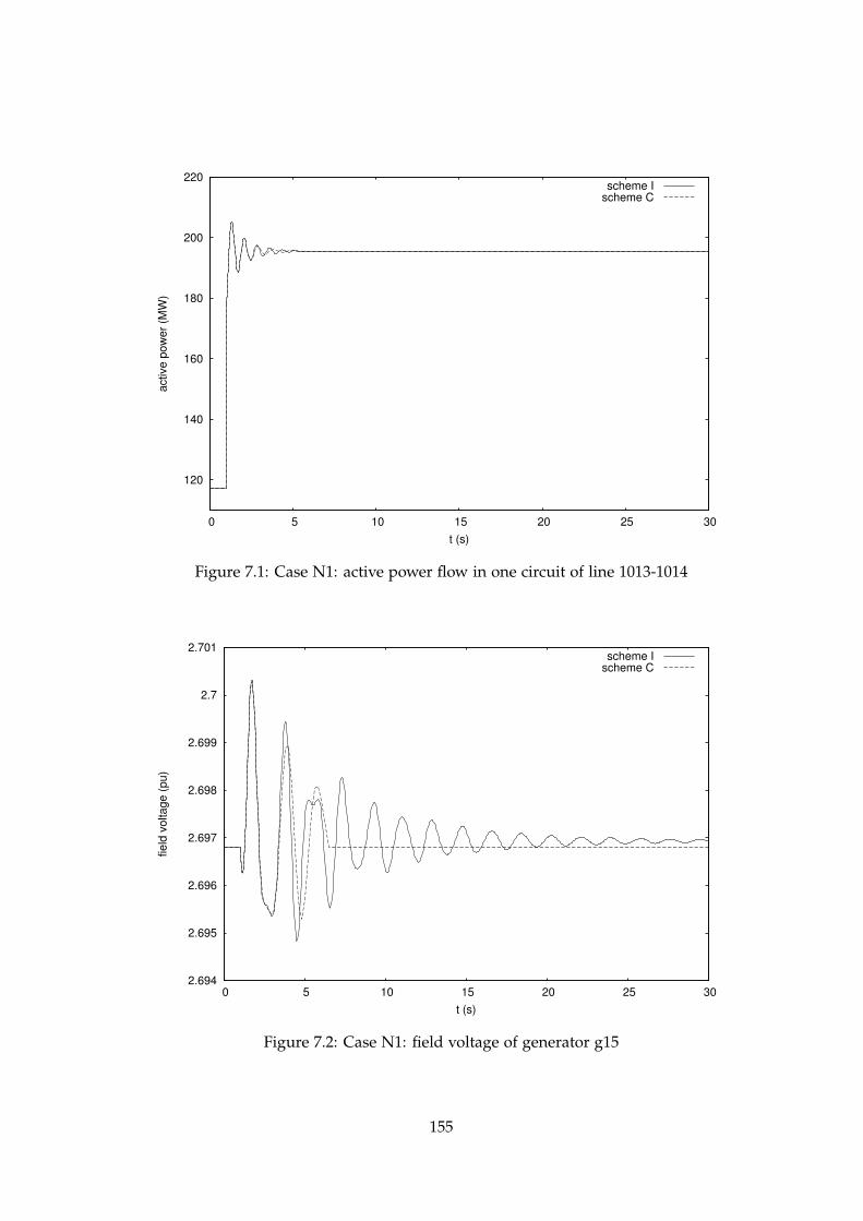
120
140
160
180
200
220
0 5 10 15 20 25 30
active p
ow
er
(MW
)
t (s)
scheme I scheme C
Figure 7.1: Case N1: active power flow in one circuit of line 1013-1014
2.694
2.695
2.696
2.697
2.698
2.699
2.7
2.701
0 5 10 15 20 25 30
field
voltage (
pu)
t (s)
scheme I scheme C
Figure 7.2: Case N1: field voltage of generator g15
155

0.97
0.975
0.98
0.985
0.99
0.995
1
0 10 20 30 40 50 60 70
voltage m
agnitude (
pu)
t (s)
scheme I scheme C
Figure 7.3: Case N2: voltage at distribution bus fed by bus 4043
2.66
2.68
2.7
2.72
2.74
2.76
2.78
2.8
2.82
2.84
0 10 20 30 40 50 60 70
field
voltage (
pu)
t (s)
scheme I scheme C
Figure 7.4: Case N2: field voltage of generator g15
156

900
950
1000
1050
1100
1150
1200
0 10 20 30 40 50 60 70
active p
ow
er
(MW
)
t (s)
scheme I scheme C
Figure 7.5: Case N2: active power produced by generator g15
0.7
0.75
0.8
0.85
0.9
0.95
1
1.05
0 20 40 60 80 100 120 140 160 180
voltage m
agnitude (
pu)
t (s)
scheme I scheme C
Figure 7.6: Case N3: voltage at transmission bus 1041
157

voltage collapse, are correctly computed, since the final discrepancy happens only when
the system is already in very stressed conditions.
Figure 7.7 provides the evolution of the speed deviation of generator g6, whose loss
of synchronism towards the end of the simulation is computed in slight advance by the
combined simulation with respect to the benchmark. As for Fig. 7.6, this is deemed of no
practical importance.
7.4.4 Case N5
Figure 7.8 provides the voltage at bus 1041, which evolves towards collapse. This case
involves a short circuit, that could not be simulated with time-averaging only because sig-
nificantly smaller steps are needed for the short-term period.
Our approach of combined simulation, however, can deal with the short-term evolution
in the same way that a detailed simulation would do, and then increase gradually the step
size. Besides a slightly accentuated damping of some oscillations, the long-term output of
scheme C matches the average behavior of the benchmark.
We can thus conclude that combined simulation is here able to deliver a reliable re-
sponse.
0
0.002
0.004
0.006
0.008
0.01
0.012
0 20 40 60 80 100 120 140 160 180
speed d
evia
tion (
pu)
t (s)
scheme I scheme C
Figure 7.7: Case N3: synchronous machine speed of generator g6
158

0.5
0.6
0.7
0.8
0.9
1
1.1
0 20 40 60 80 100 120 140 160 180
voltage m
agnitude (
pu)
t (s)
scheme I scheme C
Figure 7.8: Case N5: voltage at transmission bus 1041
7.5 Combined simulation results on Hydro-Quebec system
This section shows the results obtained with the combined simulation of the Hydro-Quebec
system, on all the scenari described in Section 2.5. The outputs have been obtained with
a dishonest Newton scheme, combining detailed simulation with localization and time-
averaging techniques (denoted “C” in the plots). More details about this and the other
solvers are given in Appendix A.5. In this scheme, after a user-imposed disturbance at
t = td, the step will be increased gradually up to its maximum value according to Table 7.3.
Table 7.3: Time step size and integration formulae used
time interval detailed simulation combined simulation[td ; td + 0.001] s 0.001 s (BEM, εL = 0) 0.001 s (BEM, εL = 0)
[td + 0.001 ; td +1
60 ] s 0.016 s (BEM, εL = 0) 0.016 s (BEM, εL = 0)[td +
160 ; td + 3.000] s 1
60 s (BDF2, εL = 0) 160 s (BDF2, εL = 0)
[td + 3.000 ; td + 9.000] s 360 s (BDF2, εL = 0) 3
60 s (BDF2, εL = 0)[td + 9.000 ; +∞] s same as above 12
60 s (BDF2, εL = 0.004)
159

7.5.1 Case Q1
The performance of scheme C in Case Q1 is identical to the performance of scheme A (see
Section 4.7.1), since the simulation spans the short-term period only.
7.5.2 Case Q2
Case Q2 allows scheme C to obtain speed-up seemingly without loss of accuracy. The
outputs of both Figs. 7.9 and 7.10 are indistinguishable from the benchmark.
7.5.3 Case Q3
Figure 7.11 provides the speed deviation of the COI, showing that the spinning reserve is
exhausted and frequency cannot be recovered close to its nominal value. Also in this case,
the outputs of scheme C fully preserve the accuracy.
7.5.4 Case Q4
Case Q4 is particularly interesting owing to the marginal activation of one MAIS device,
similar to the ones mentioned in previous chapters. Figure 7.12 shows a zoom of the voltage
evolution at bus 755 with the indication of the switching threshold. The MAIS device
switches off the reactor if the voltage stays below the threshold for 13 s consecutively. The
output computed with scheme I stays below the threshold for slightly less than 9 s, thus
triggering no MAIS tripping, while the output computed with scheme C, conversely, stays
below the threshold for just a slightly longer time than 13 s, the tripping delay. This results
in 4 MAIS activations in scheme I and 5 in scheme C. As already mentioned, a mistake in
the identification of one MAIS device is not considered critical in the context of DSA.
The variable of interest for this case is the voltage at transmission bus 702, provided in
Fig. 7.13.
7.5.5 Case Q5
Figure 7.14 shows the zoomed evolution of voltage at faulted bus 702. The action of the third
MAIS device, at bus 730, is anticipated by scheme C by some ten seconds, which makes the
second and third MAIS devices act nearly simultaneously. This produces a 5 s anticipation
of the fourth (and last) MAIS move, but ultimately no difference in the number of MAIS
160

-0.007
-0.006
-0.005
-0.004
-0.003
-0.002
-0.001
0
0 20 40 60 80 100
speed d
evia
tion (
pu)
t (s)
scheme I scheme C
Figure 7.9: Case Q2: deviation of COI speed
-0.025
-0.02
-0.015
-0.01
-0.005
0
0.005
0.01
0 20 40 60 80 100
dvpss (
pu)
t (s)
scheme I scheme C
Figure 7.10: Case Q2: PSS signal of generator 294
161

-0.016
-0.014
-0.012
-0.01
-0.008
-0.006
-0.004
-0.002
0
0 20 40 60 80 100
speed d
evia
tion (
pu)
t (s)
scheme I scheme C
Figure 7.11: Case Q3: deviation of COI speed
0.96
0.965
0.97
0.975
0.98
55 60 65 70 75 80 85
voltage m
agnitude (
pu)
t (s)
scheme I scheme C
MAIS switching threshold
Figure 7.12: Case Q4: zoom of the voltage evolution at transmission bus 755
162
0.95
0.955
0.96
0.965
0.97
0.975
0.98
0.985
0.99
0.995
1
0 50 100 150 200 250 300
voltage m
agnitude (
pu)
t (s)
scheme I scheme C
Figure 7.13: Case Q4: voltage at transmission bus 702
0.96
0.965
0.97
0.975
0.98
0.985
0.99
0 50 100 150 200 250 300
voltage m
agnitude (
pu)
t (s)
scheme I scheme C
Figure 7.14: Case Q5: zoom of the voltage evolution at transmission bus 702
163

activations. Again, the discrepancy due to a marginal switch of such a large-impact discrete
device is deemed fully acceptable.
7.5.6 Computational effort
Table 7.4 summarizes the gain in computing time which is obtained with scheme C com-
pared to scheme I, while preserving an acceptable level of accuracy. The performance of
schemes T, A and L are repeated as well to give a general view over all the proposed
techniques. The combination of decomposition, localization and time-averaging brings a
significant speed-up ratio in the simulation of long-term cases (i.e. Q2, Q3, Q4 and Q5),
which ranges from 4 to 7 with respect to the benchmark.
Table 7.4: CPU times (s)
Case Scheme I Scheme T Scheme A Scheme L Scheme CεL = 0.001
Q1 11.11 5.93 6.04 5.93Q2 35.84 10.53 11.91 11.06 4.76Q3 27.89 9.91 13.16 12.19 5.40Q4 60.16 23.79 30.55 28.51 10.63Q5 61.34 34.36 32.80 13.80
7.6 Combined simulation results on PEGASE system
This section shows the results obtained with the combined simulation of the PEGASE test
system, in all the scenari described in Section 2.6. The outputs have been obtained with
a dishonest Newton scheme, combining detailed simulation with localization and time-
averaging techniques (denoted “C” in the plots). More details about this and the other
solvers are given in Appendix A.5. In this scheme, after a user-imposed disturbance at
t = td, the step will be increased gradually up to its maximum value according to Table 7.5.
7.6.1 Cases P1, P2 and P3
The voltage evolutions at bus F0322411 are shown in Figs. 7.15, 7.16, 7.17 and 7.18 for the
three scenari. The approximation brought by combined simulation yields very satisfactory
results.
164

0.98
0.99
1
1.01
1.02
1.03
1.04
1.05
0 5 10 15 20
voltage m
agnitude (
pu)
t (s)
scheme I scheme C
Figure 7.15: Case P1: voltage at transmission bus F0322411
0.99
1
1.01
1.02
1.03
1.04
1.05
0 50 100 150 200
voltage m
agnitude (
pu)
t (s)
scheme I scheme C
Figure 7.16: Case P2: voltage at transmission bus F0322411
165

0.96
0.98
1
1.02
1.04
1.06
0 2 4 6 8 10
voltage m
agnitude (
pu)
t (s)
scheme I scheme C
Figure 7.17: Case P3: zoom of the short-term voltage evolution at transmission bus F0322411
1.01
1.015
1.02
1.025
1.03
0 50 100 150 200
voltage m
agnitude (
pu)
t (s)
scheme I scheme C
Figure 7.18: Case P3: zoom of the long-term voltage evolution at transmission bus F0322411
166

Table 7.5: Time step size and integration formulae used
time interval detailed simulation combined simulation[td ; td + 0.001] s 0.001 s (BEM, εL = 0) 0.001 s (BEM, εL = 0)
[td + 0.001 ; td + 0.010] s 0.009 s (BEM, εL = 0) 0.009 s (BEM, εL = 0)[td + 0.010 ; td + 0.170] s 0.010 s (BDF2, εL = 0) 0.010 s (BDF2, εL = 0)[td + 0.170 ; td + 0.450] s 0.020 s (BDF2, εL = 0) 0.020 s (BDF2, εL = 0)[td + 0.450 ; td + 1.200] s 0.050 s (BDF2, εL = 0) 0.050 s (BDF2, εL = 0)[td + 1.200 ; td + 2.400] s same as above 0.100 s (BDF2, εL = 0)[td + 2.400 ; td + 5.000] s same as above 0.200 s (BDF2, εL = 0)
[td + 5.000 ; +∞] s same as above 0.500 s (BDF2, εL = 0.01)
7.6.2 Computational effort
Tables 7.6 and 7.7 detail the computing times obtained and the number of operations per-
formed in case P1 using the benchmark scheme I and scheme C, respectively. The per-
formance of schemes T, A and L are repeated as well to give a general view over all the
proposed techniques. Similar results for Case P2 are given in Tables 7.8 and 7.9, for Case
P3 in Tables 7.10 and 7.11. All the tables show that the respective gains gain brought by
time-averaging and localization can be successfully combined.
Figures 7.19 and 7.20 show the plots of the elapsed time vs. the simulation time. The
bisectrix y = x represents a simulation as fast as real-time (1:1 ratio between elapsed and
simulation time), while a curve below the diagonal corresponds to simulation faster than
real-time. Apart from the initial transients, scheme C is indeed faster than real-time in both
cases. The other schemes are plotted to give a complete view of the presented techniques.
7.7 Chapter conclusion
This chapter hosts the final contribution of this thesis, which is a combination of detailed
simulation and accuracy relaxation techniques applied to the decomposed dishonest New-
ton solution: to our knowledge, the reported gains in CPU time are unprecedented in
long-term dynamic simulation of power systems of the size of PEGASE, on single-core com-
puters, while avoiding to develop a simplified model. The gain obtained in the short-term
scenario is also significant, thanks mainly to the techniques detailed in Chapter 4.
In the PEGASE system the gain of scheme C ranges between 6 and 16, while in Hydro-
Quebec system is between 2 and 7, with respect to scheme I. A solver approaching real-time
and retaining a satisfactory accuracy is within reach thanks to the presented techniques.
167

0
50
100
150
200
250
300
350
400
450
0 50 100 150 200
ela
psed tim
e (
s)
simulation time (s)
real-time scheme I
scheme A scheme L, epsilon_L=0.0025
scheme T, h=0.5 scheme C
Figure 7.19: Case P2: elapsed time vs. simulation time
0
50
100
150
200
250
300
350
400
450
0 50 100 150 200
ela
psed tim
e (
s)
simulation time (s)
real-time scheme I
scheme A scheme L, epsilon_L=0.0025
scheme C
Figure 7.20: Case P3: elapsed time vs. simulation time
168
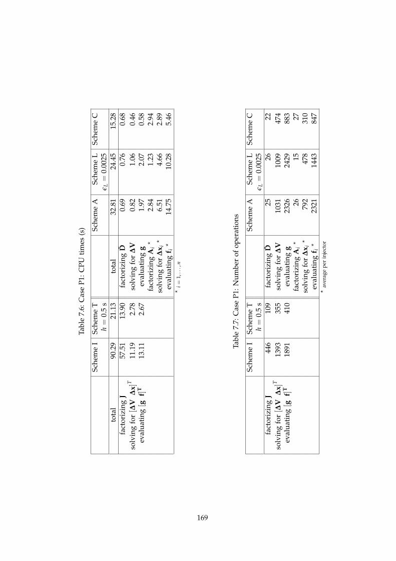
Tabl
e7.
6:C
ase
P1:C
PUti
mes
(s)
Sche
me
ISc
hem
eT
Sche
me
ASc
hem
eL
Sche
me
Ch=
0.5
sε L
=0.
0025
tota
l90
.29
21.1
3to
tal
32.8
124
.45
15.2
8fa
ctor
izin
gJ
57.5
113
.90
fact
oriz
ing
D0.
690.
760.
68so
lvin
gfo
r[∆
V∆
x]T
11.1
92.
78so
lvin
gfo
r∆
V0.
821.
060.
46ev
alua
ting
[gf]
T13
.11
2.67
eval
uati
ngg
1.97
2.07
0.58
fact
oriz
ing
Ai?
2.84
1.23
2.94
solv
ing
for
∆x i
?6.
514.
662.
89ev
alua
ting
f i?
14.7
510
.28
5.46
?i=
1,..
.,n
Tabl
e7.
7:C
ase
P1:N
umbe
rof
oper
atio
ns
Sche
me
ISc
hem
eT
Sche
me
ASc
hem
eL
Sche
me
Ch=
0.5
sε L
=0.
0025
fact
oriz
ing
J44
610
9fa
ctor
izin
gD
2526
22so
lvin
gfo
r[∆
V∆
x]T
1393
355
solv
ing
for
∆V
1031
1009
474
eval
uati
ng[g
f]T
1891
410
eval
uati
ngg
2326
2429
883
fact
oriz
ing
Ai?
2615
27so
lvin
gfo
r∆
x i?
792
478
310
eval
uati
ngf i
?23
2114
4384
7?
aver
age
per
inje
ctor
169

Tabl
e7.
8:C
ase
P2:C
PUti
mes
(s)
Sche
me
ISc
hem
eT
Sche
me
ASc
hem
eL
Sche
me
Ch=
0.5
sε L
=0.
0025
tota
l47
0.00
105.
89to
tal
220.
2113
2.41
30.0
7fa
ctor
izin
gJ
207.
5868
.80
fact
oriz
ing
D0.
750.
960.
75so
lvin
gfo
r[∆
V∆
x]T
90.0
013
.86
solv
ing
for
∆V
7.42
8.25
1.41
eval
uati
ng[g
f]T
111.
8613
.38
eval
uati
ngg
14.0
414
.66
2.11
fact
oriz
ing
Ai?
2.51
1.25
2.11
solv
ing
for
∆x i
?41
.53
20.7
36.
05ev
alua
ting
f i?
117.
2554
.76
12.3
1?
i=1,
...,
n
Tabl
e7.
9:C
ase
P2:N
umbe
rof
oper
atio
ns
Sche
me
ISc
hem
eT
Sche
me
ASc
hem
eL
Sche
me
Ch=
0.5
sε L
=0.
0025
fact
oriz
ing
J15
9751
1fa
ctor
izin
gD
2732
24so
lvin
gfo
r[∆
V∆
x]T
1110
617
04so
lvin
gfo
r∆
V85
1484
7616
31ev
alua
ting
[gf]
T15
988
2196
eval
uati
ngg
1716
018
310
2753
fact
oriz
ing
Ai?
2216
20so
lvin
gfo
r∆
x i?
5634
2089
685
eval
uati
ngf i
?19
044
7192
1842
?av
erag
epe
rin
ject
or
170

Tabl
e7.
10:C
ase
P3:C
PUti
mes
(s)
Sche
me
ISc
hem
eA
Sche
me
LSc
hem
eC
ε L=
0.00
25to
tal
438.
21to
tal
232.
5617
4.35
41.2
9fa
ctor
izin
gJ
179.
40fa
ctor
izin
gD
0.93
1.03
0.94
solv
ing
for[∆
V∆
x]T
88.9
3so
lvin
gfo
r∆
V8.
197.
831.
80ev
alua
ting
[gf]
T11
1.34
eval
uati
ngg
13.9
114
.32
2.53
fact
oriz
ing
Ai?
4.49
2.56
4.65
solv
ing
for
∆x i
?47
.35
29.6
98.
64ev
alua
ting
f i?
119.
4483
.23
16.0
4?
i=1,
...,
n
Tabl
e7.
11:C
ase
P3:N
umbe
rof
oper
atio
ns
Sche
me
ISc
hem
eA
Sche
me
LSc
hem
eC
ε L=
0.00
25fa
ctor
izin
gJ
1374
fact
oriz
ing
D32
3428
solv
ing
for[∆
V∆
x]T
1097
5so
lvin
gfo
r∆
V85
5683
6218
87ev
alua
ting
[gf]
T15
946
eval
uati
ngg
1702
017
337
3165
fact
oriz
ing
Ai?
4027
43so
lvin
gfo
r∆
x i?
5757
3429
893
eval
uati
ngf i
?19
285
1157
225
09?
aver
age
per
inje
ctor
171


Chapter8
General conclusion
The value of an idea
lies in the using of it 1
8.1 Summary of work and main contributions
In this work methods to speed up time-domain simulations of large-scale power systems
have been proposed, a typical application being dynamic security assessment. We summa-
rize hereafter the main contributions.
The advantages of a non-causal equation-based hybrid modelling have been stressed.
It allows intuitive writing of both physical constraints and control equations, regardless
whether they are algebraic or differential, continuous or discrete. Since no causality is
imposed, an equation can dynamically change from differential to algebraic and viceversa.
This feature has been exploited in the treatment of state events. Also, an explicit center-of-
inertia reference frame has been proposed for use in long-term simulations.
The heart of the proposed techniques is a decomposition of the linear equations solved
at each Newton iteration, exploiting the bordered block-diagonal structure of the Jacobian
matrix. Algorithms have been proposed to minimize the number of partial Jacobian up-
dates and re-factorizations, and perform less iterations on components with lower dynamic
1Thomas Alva Edison, in an interview given to E. Hubbard, published in [HB28].
173

response. The accuracy and convergence properties of the original Newton method are
preserved at this stage.
Further speed-ups have been obtained by relaxing accuracy to an extent compatible with
applications such as dynamic security assessment. The overall approach offers the impor-
tant advantage of using the same model as detailed simulations. Hence, model reduction
or simplification is not required; instead, the gain in efficiency comes from the relaxable
accuracy solver used to simulate the reference model.
Accuracy has been first relaxed in space, by localizing the system response. Localization
exploits the fact that, in a large-scale system, most of disturbances give rise to localized
effects, i.e. some system components do not participate much in the dynamic response.
Latent components are not solved, but replaced by a static linear model relating injected
current to bus voltage.
Accuracy has been also relaxed in time by numerically averaging the system response.
Time-averaging is obtained by using a step size which is large with respect to the dynamics
that are deemed negligible for the application of concern. To this purpose, attention has
been paid to the handling of discrete dynamics, performed without identifying the exact
instant of the discrete transition, but with an ex post treatment of discrete events.
Our final recommendation to achieve faster simulations, the focus being on the long-
term response of the system to the initiating disturbance, is a combination of detailed dy-
namic simulation in the short-term with relaxation of accuracy in the long-term by means of
localization and time averaging. The advantage of the proposed method lies in the seamless
integration between detailed short-term simulation and relaxed-accuracy long-term simu-
lation, one disadvantage being hyper-stability, which may lead to overlooking instability
of oscillations. Tests performed on large-scale systems indicate that very significant reduc-
tions in computing time can be obtained when combining the techniques of decomposition,
localization and time-averaging, which are the most salient contributions of this thesis.
The results presented in this report were obtained with a mock-up developed at the
University of Liege. A wide variety of grids has been considered, namely (i) the Nordic32
system, an academic test system, (ii) the Hydro-Quebec system, a real system with 11774
differential-algebraic states, and (iii) within the context of a European project, the PEGASE
system, whose size is unprecedented with a total number of 146239 differential-algebraic
states.
Most of the corresponding algorithms have been subsequently implemented in a dy-
174

namic simulation prototype derived from EUROSTAG [SBDB89] and, for some of them, in
a dispatch training simulator prototype based on FAST-DTS [GCA+00].
8.2 Directions for future work
The presented algorithms may be expanded and further improved along the following di-
rections:
• mitigating or bounding the risks coming from the hyper-stability of the presently used
integration methods (namely backward differentiation formulae);
• investigating heuristics for automatic switching between detailed, short-term simula-
tion and relaxed-accuracy, long-term simulation;
• investigating techniques for estimating and controlling of the simulation error, for
instance through numerical estimations based on Newton iteration count;
• extending the decomposed formulation to multi-terminal HVDC networks with the
introduction of internal DC buses into a mixed AC/DC network;
• using the proposed techniques to assess the feasibility of a real implementation of dy-
namic security assessment, for instance to determine secure operation limits [VVC06].
The work performed in this thesis has also served as a basis for extensions that are being
investigated in collaboration with other researchers of the University of Liege:
• using multi-layer domain decomposition algorithms, such as sub-tree reduction method,
in order to include distribution networks, whose impact on power system dynamics
is likely to increase with the installation of dispersed generation1;
• including detailed power electronics models into dynamic simulation under the pha-
sor approximation within the proposed injector-network domain decomposition BBD
framework, using multi-rate techniques to interface the currents computed with an
1See P. Aristidou, D. Fabozzi, and T. Van Cutsem. A Schur complement method for DAE systems in powersystem simulation. Accepted for presentation in 21st International Conference on Domain Decomposition Methods,Rennes, France, June 2012.
175

electromagnetic transients program with the main transmission network represented
in the phasor domain1;
• parallelizing the computations dealing with injectors for use on multi-core processor
architectures, which are becoming increasingly common even in off-the-shelf hard-
ware, and are likely to be the most effective near-future way of increasing computa-
tional power2.
1See F. Plumier, D. Fabozzi, C. Geuzaine, and T. Van Cutsem. Combining full transients and phasor ap-proximation models in power system time simulation. Accepted for presentation in 21st International Conference onDomain Decomposition Methods, Rennes, France, June 2012.
2See P. Aristidou, D. Fabozzi, and T. Van Cutsem. Dynamic simulations of large-scale power systems onparallel architectures using a domain decomposition method. Submitted for publication in IEEE Transactions onParallel and Distributed Systems, 2012.
176

Appendices
Der liebe Gott steckt im Detail 1
A.1 Explicit reference frame [FVC11b]
The continuous part of the dynamic model of an electric power system considered in sta-
bility studies can be written as shown in Chapter 2 and repeated here for clarity:
0 = D V− C x (A.1)
Γ(z) x = φ(x, z, V) (A.2)
Equations (A.1) relate to the network, whose response is assumed instantaneous under
the phasor approximation. It is appropriate to project these complex equations onto two
orthogonal axes, denoted x and y, respectively. Equations (A.2) deal with a variety of short-
and long-term phenomena and controls, with corresponding state variables in x. Among
them, the motion of the rotor of i-th synchronous machine (i = 1, . . . , m) is described by:
θi = ωi (A.3)
Miωi = Tmi − Tei (A.4)
1God is in the detail. Apocryphal, attributed to art historian Abraham Moritz (Aby) Warburg among others.Also used in its dual form: der Teufel (”devil”) steckt im Detail.
177

where Mi is an inertia coefficient, Tmi (resp. Tei) is the turbine mechanical (resp. generator
electromagnetic) torque, ωi is the rotor speed and θi the rotor position with respect to a
fixed reference.
Apart from the need to have all phase angles referring to the same axis, the choice of
the latter is free. In fact, all variables in x except angles are unaffected by this choice. The x
and y axes should be chosen having in mind computational efficiency.
A standard practice is to choose axes that rotate at the nominal angular frequency ωo =
2π fo, where fo is the nominal frequency of the system. The rotor angle of the i-th machine,
referred to the x-axis is:
δi = θi − (ωot + C) (A.5)
where C is an arbitrary constant. This yields:
δi = ωi −ωo (A.6)
This equation is substituted to (A.3), while (A.4) is unchanged.
While appropriate for short-term simulations (e.g. for transient stability analysis), the
above reference suffers from a major drawback in long-term studies. Indeed, after a dis-
turbance affecting the power balance, the system settles at a new angular frequency ω and,
with respect to the reference axes, all phasors rotate at the angular speed ω − ωo. Hence,
although the system settles at a new equilibrium, the δi variable increase linearly with time
and the components of vx, vy, ix and iy oscillate with a period T = 2π|ω−ωo|−1. This non-
linear behaviour requires frequent updates of the Jacobian matrix and increases the number
of iterations of the Newton method used to solve the implicit equations. It also requires the
time step to remain small compared to T, in order to track those oscillations and/or avoid
numerical instability.
The above problem can be solved by somewhat linking the references axes to the rotor
motion. This is the idea underlying the Center-Of-Inertia (COI) reference frame, which has
been used in direct transient stability analysis methods [TS72] and in industrial simulation
software (e.g. [SBDB89]). The COI angle and its time derivative are defined respectively as:
θcoi =1
MT
m
∑i=1
Miθi + K (A.7)
ωcoi =1
MT
m
∑i=1
Miωi (A.8)
where MT = ∑mi=1 Mi is the total inertia and K is an arbitrary constant. The x and y axes
now turn at the angular speed ωcoi. The rotor angle of the i-th machine, referred to the
178

x-axis is:
δi = θi − θcoi (A.9)
from which one easily derives:
δi = θi − θcoi = ωi −ωcoi (A.10)
This equation replaces (A.3). Thus, in an m-machine system, there are m equations of
the type (A.10) involving m state variables δi and the (m + 1)-th variable ωcoi. The latter
is included in y and is balanced by (A.8), an algebraic equation handled by the Newton
method together with (A.1). Note that (A.8) can be replaced by ∑mi=1 Miδi = 0.
Clearly, if the system settles at a new equilibrium with frequency f , all machines rotate
at the angular speed 2π f and so does the x axis. Hence, vx, vy, ix and iy become constant.
This result still holds true when substituting to the right hand side of (A.8) a linear
combination ∑mi=1 aiωi with ∑m
i=1 ai = 1, and in particular a single reference speed. The
COI frame of reference, however, is appealing as it provides the average system angular
frequency. The latter is appropriately used in frequency-dependant load models as well as
in corrective damping terms Di(ωi −ωcoi) added to (A.4).
Still, this COI reference suffers from drawbacks. First, the presence of ωcoi in each
equation (A.10) and in the load models produces a dense column in the Jacobian matrix,
while the presence of all ωi’s in (A.8) produces a “dense” row. Next, in case of network
split, since one COI has to be considered in each connected subnetwork, the structure of
the Jacobian is significantly modified by the added variables and equations. Finally, the
algebraic equation (A.8) does not allow to take advantage of the block bordered diagonal
structure of the Jacobian, as detailed in Chapter 4.
We propose an explicit approach which is free from these drawbacks. The idea is to
make the x axis coincide with a previous position of the COI. In the context of numerical
simulation, when integrating the equations from t− h to t (where h is the time step), the
phasors are projected onto axes that correspond to the COI position at t− h. At that time,
the COI speed is ωcoi(t− h). The angle and speed of the i-th machine, referred to that axis
become:
δi = θi − θcoi(t− h) (A.11)
δi = ωi −ωcoi(t− h) (A.12)
179

Note that the COI considered in (A.10) is “implicit” in the sense that it involves the
rotor speeds at the same time t, while the one considered in (A.12) is “explicit” in so far
as it refers to past, already known speed values. In (A.12), ωcoi(t − h) is just a number,
not a variable. Equation (A.8) is not handled together with the other equations. It is used,
after convergence of the Newton iterations, to determine the value of ωcoi(t) from the just
computed rotor speeds ωi(t). This updated value of ωcoi is used in (A.12) when proceeding
with the next integration step.
By so doing, the dense row and column are no longer present in the Jacobian, while
network splits do not require any restructuring of the Jacobian.
The advantages of the COI reference frame are also preserved, because a slightly delayed
COI angle is as good as the exact COI in making vx, vy, ix and iy very little dependent on
the system frequency. One could argue that using a slightly delayed ωcoi in the frequency
dependent load models causes some inaccuracy; however, using ωcoi instead of the true
angular frequency at the load bus already involves some approximation.
To show the effectiveness of the method we consider a variant of the system used in
[FVC09], subject to a branch outage. All responses have been computed using the Trape-
zoidal method with h = 0.01 s.
The long-term evolution of a bus voltage magnitude is shown in Fig. A.1. The system
responds to an overexcitation limiter acting at t ' 50 s and a transformer load tap changer
moving by 10 steps, before hitting its limit.
The evolution of ωcoi is shown in Fig. A.2. The overall increase is due to the load
sensitivity to the dropping voltage. As can be seen, the system settles at equilibrium after
t ' 120 s.
Apart from imperceptible numerical inaccuracies (within the solver tolerances), ωcoi is
the same, whichever angle reference is used, since the ωi’s are also the same.
Figure A.3 shows with dotted line the evolution of the vx component of the same bus
voltage, when using the angle reference as in (A.5). As expected, vx undergoes pronounced
oscillations, even after the frequency has returned to steady state. The other two curves
have been obtained with the angle references defined by (A.10) and (A.12), respectively. The
corresponding reference axes differ by the angle∫ t
t−h ωcoi(u) du = θcoi(t)− θcoi(t− h), which
is small for h = 0.01 s, and hence makes the curves indistinguishable. More importantly,
these two curves are much smoother than the first one.
180

0.84
0.86
0.88
0.9
0.92
0.94
0.96
0.98
1
1.02
0 50 100 150 200
volta
ge m
agni
tude
(pu
)
t (s)
Figure A.1: Evolution of voltage
0.9998
1
1.0002
1.0004
1.0006
1.0008
1.001
1.0012
1.0014
0 50 100 150 200
angu
lar
spee
d (p
u)
t (s)
Figure A.2: Evolution of COI angular speed
181

-1
-0.5
0
0.5
1
0 50 100 150 200
vx c
ompo
nent
of v
olta
ge (
pu)
t (s)
Eqs. ( A.9,A.10)Eqs. (A.11,A.12)Eqs. ( A.5, A.6)
Figure A.3: Evolution of a vx component
.
182

A.2 Synchronous machine model
The advantages of equation-based over input-output modelling mentioned in Section 2.2
can be clarified with a power system example: the synchronous machine model including
saturation effects. In order to have a single model, whatever the number of rotor windings,
we use “model switches”, i.e. integer parameters such as Sd1 = 1 if there is a damper
winding d1, Sd1 = 0 otherwise, and similarly for q1 and q2.
The table below shows usual models and their corresponding values of switches:
model switchesdetailed, round rotor Sd1 = 1, Sq1 = 1, Sq2 = 1detailed, salient pole Sd1 = 1, Sq1 = 1, Sq2 = 0
simplified, no damper Sd1 = 0, Sq1 = 0, Sq2 = 0
Using the equal-mutual-flux-linkage per unit system, the relationship between magnetic
flux linkages and currents can be written as:ψd
ψ f
ψd1
=
L` + Md Md Sd1Md
Md L` f + Md Sd1Md
Sd1Md Sd1Md L`d1 + Sd1Md
id
i f
id1
ψq
ψq1
ψq2
=
L` + Mq Sq1Mq Sq2Mq
Sq1Mq L`q1 + Sq1Mq Sq2Mq
Sq2Mq Sq2Mq L`q2 + Sq2Mq
iq
iq1
iq2
The d and q components of the air-gap flux are given by:
ψad = Md(id + i f + Sd1id1) (A.13)
ψaq = Mq(iq + Sq1iq1 + Sq2iq2) (A.14)
From the above equations, and taking into account that the S variables can take values
in {0, 1} only, one easily obtains:
ψd = L`id + ψad (A.15)
ψ f = L` f i f + ψad (A.16)
ψd1 = L`d1id1 + Sd1ψad (A.17)
ψq = L`iq + ψaq (A.18)
ψq1 = L`q1iq1 + Sq1ψaq (A.19)
ψq2 = L`q2iq2 + Sq2ψaq (A.20)
183
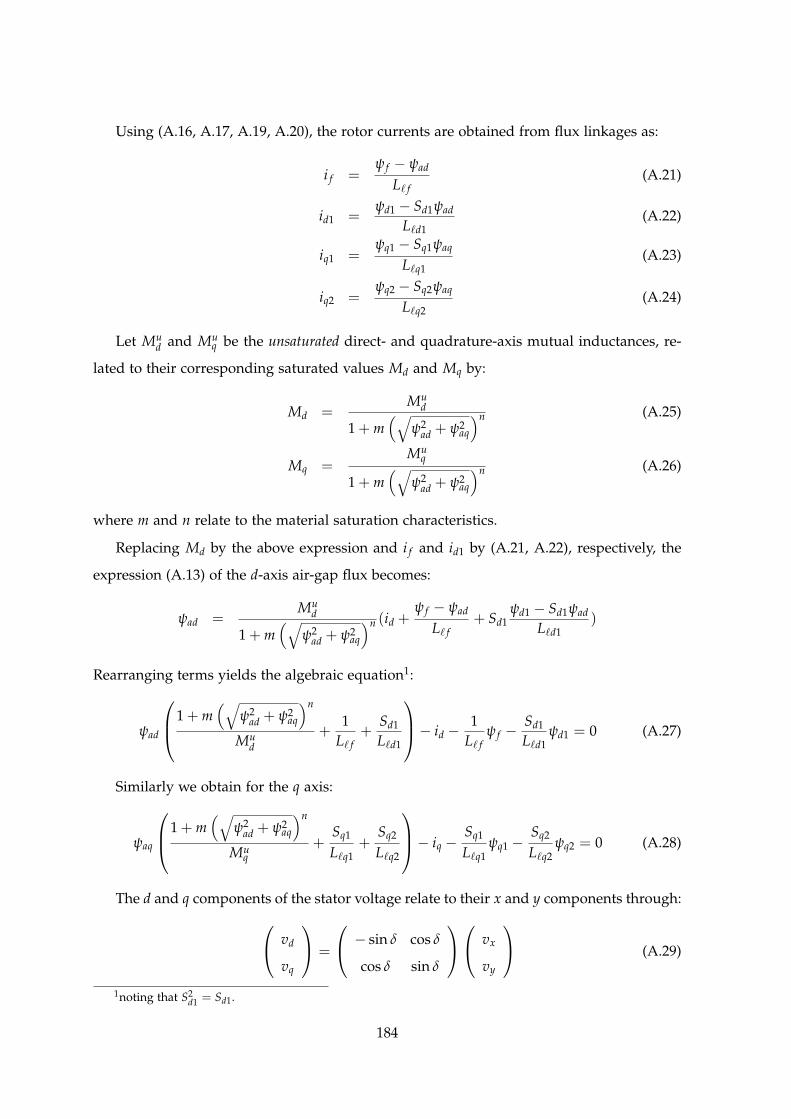
Using (A.16, A.17, A.19, A.20), the rotor currents are obtained from flux linkages as:
i f =ψ f − ψad
L` f(A.21)
id1 =ψd1 − Sd1ψad
L`d1(A.22)
iq1 =ψq1 − Sq1ψaq
L`q1(A.23)
iq2 =ψq2 − Sq2ψaq
L`q2(A.24)
Let Mud and Mu
q be the unsaturated direct- and quadrature-axis mutual inductances, re-
lated to their corresponding saturated values Md and Mq by:
Md =Mu
d
1 + m(√
ψ2ad + ψ2
aq
)n (A.25)
Mq =Mu
q
1 + m(√
ψ2ad + ψ2
aq
)n (A.26)
where m and n relate to the material saturation characteristics.
Replacing Md by the above expression and i f and id1 by (A.21, A.22), respectively, the
expression (A.13) of the d-axis air-gap flux becomes:
ψad =Mu
d
1 + m(√
ψ2ad + ψ2
aq
)n (id +ψ f − ψad
L` f+ Sd1
ψd1 − Sd1ψad
L`d1)
Rearranging terms yields the algebraic equation1:
ψad
1 + m(√
ψ2ad + ψ2
aq
)n
Mud
+1
L` f+
Sd1
L`d1
− id −1
L` fψ f −
Sd1
L`d1ψd1 = 0 (A.27)
Similarly we obtain for the q axis:
ψaq
1 + m(√
ψ2ad + ψ2
aq
)n
Muq
+Sq1
L`q1+
Sq2
L`q2
− iq −Sq1
L`q1ψq1 −
Sq2
L`q2ψq2 = 0 (A.28)
The d and q components of the stator voltage relate to their x and y components through: vd
vq
=
− sin δ cos δ
cos δ sin δ
vx
vy
(A.29)
1noting that S2d1 = Sd1.
184

and similarly for the current: id
iq
=
− sin δ cos δ
cos δ sin δ
ix
iy
(A.30)
where δ is the rotor angle (angle between q axis and the reference detailed in Appendix A.1).
Eqs. (A.27, A.28) become respectively:
ψad
1 + m(√
ψ2ad + ψ2
aq)n
Mud
+1
L` f+
Sd1
L`d1
+ sin δ ix− cos δ iy−1
L` fψ f −
Sd1
L`d1ψd1 = 0 (A.31)
Similarly we obtain for the q axis:
ψaq
1 + m(√
ψ2ad + ψ2
aq)n
Muq
+Sq1
L`q1+
Sq2
L`q2
− cos δ ix − sin δ iy −Sq1
L`q1ψq1 −
Sq2
L`q2ψq2 = 0
(A.32)
The original Park equations are written as:
vd = −Raid −ωNψq (A.33)
vq = −Raiq + ωNψd (A.34)dψ f
dt= ωN(K f v f − R f i f ) (A.35)
dψd1
dt= −ωN Rd1id1 (A.36)
dψq1
dt= −ωN Rq1iq1 (A.37)
dψq2
dt= −ωN Rq2iq2 (A.38)
The stator equations are transformed as follows. Eqs. (A.30) are used to express vd, vq,
id and iq as functions of vx, vy, ix, iy, while Eqs. (A.15, A.18) are used to involve ψad and
ψaq. This yields for the d axis:
vd = −Ra(− sin δ ix + cos δ iy)−ωN(L`iq + ψaq)
= −Ra(− sin δ ix + cos δ iy)−ωN L`(cos δ ix + sin δ iy)−ωNψaq
and finally:
0 = sin δvx − cos δvy + (Ra sin δ−ωN L` cos δ)ix − (Ra cos δ + ωN L` sin δ)iy −ωNψaq (A.39)
For the q axis we have:
vq = −Ra(cos δ ix + sin δ iy) + ωN(L`id + ψad)
= −Ra(cos δ ix + sin δ iy) + ωN L`(− sin δ ix + cos δ iy) + ωNψad
185
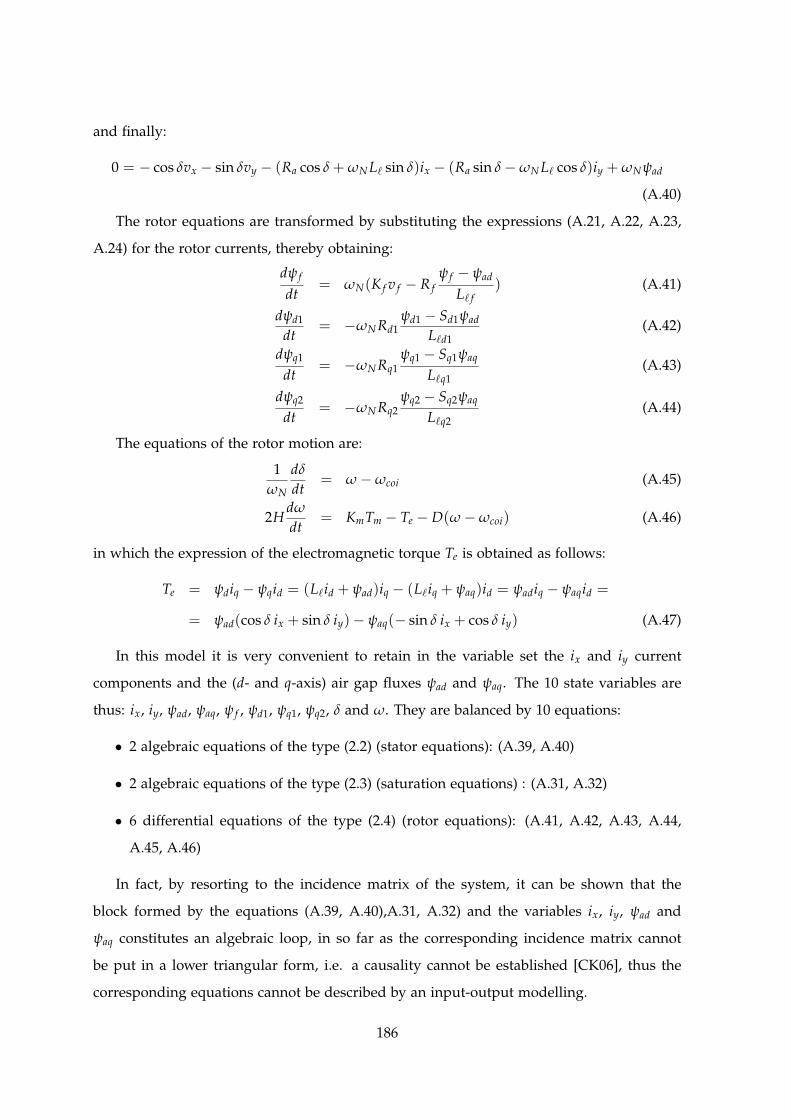
and finally:
0 = − cos δvx − sin δvy − (Ra cos δ + ωN L` sin δ)ix − (Ra sin δ−ωN L` cos δ)iy + ωNψad
(A.40)
The rotor equations are transformed by substituting the expressions (A.21, A.22, A.23,
A.24) for the rotor currents, thereby obtaining:
dψ f
dt= ωN(K f v f − R f
ψ f − ψad
L` f) (A.41)
dψd1
dt= −ωN Rd1
ψd1 − Sd1ψad
L`d1(A.42)
dψq1
dt= −ωN Rq1
ψq1 − Sq1ψaq
L`q1(A.43)
dψq2
dt= −ωN Rq2
ψq2 − Sq2ψaq
L`q2(A.44)
The equations of the rotor motion are:
1ωN
dδ
dt= ω−ωcoi (A.45)
2Hdω
dt= KmTm − Te − D(ω−ωcoi) (A.46)
in which the expression of the electromagnetic torque Te is obtained as follows:
Te = ψdiq − ψqid = (L`id + ψad)iq − (L`iq + ψaq)id = ψadiq − ψaqid =
= ψad(cos δ ix + sin δ iy)− ψaq(− sin δ ix + cos δ iy) (A.47)
In this model it is very convenient to retain in the variable set the ix and iy current
components and the (d- and q-axis) air gap fluxes ψad and ψaq. The 10 state variables are
thus: ix, iy, ψad, ψaq, ψ f , ψd1, ψq1, ψq2, δ and ω. They are balanced by 10 equations:
• 2 algebraic equations of the type (2.2) (stator equations): (A.39, A.40)
• 2 algebraic equations of the type (2.3) (saturation equations) : (A.31, A.32)
• 6 differential equations of the type (2.4) (rotor equations): (A.41, A.42, A.43, A.44,
A.45, A.46)
In fact, by resorting to the incidence matrix of the system, it can be shown that the
block formed by the equations (A.39, A.40),A.31, A.32) and the variables ix, iy, ψad and
ψaq constitutes an algebraic loop, in so far as the corresponding incidence matrix cannot
be put in a lower triangular form, i.e. a causality cannot be established [CK06], thus the
corresponding equations cannot be described by an input-output modelling.
186

A.3 Restorative load model
The advantages of hybrid equation-based over input-output modelling outlined in Sec-
tion 2.3 can be clarified with a power system example: the model of the restorative load
which has been used in this thesis.
A.3.1 Continuous part of the model
Consider first an admittance load with the following relationships between power and volt-
age:
P = P0
(VV0
)2
xp = (V2x + V2
y )P0
V20
xp (A.48)
Q = Q0
(VV0
)2
xq = (V2x + V2
y )Q0
V20
xq (A.49)
where V0, P0 and Q0 refer to the initial values of voltage V, active power P and reactive
power Q, and the role of xp and xq will be explained in the sequel.
Substituting P and Q with their expressions in terms of voltage (Vx, Vy) and current
(ix, iy) in Cartesian coordinates yields:
Vxix + Vyiy = (V2x + V2
y )P0
V20
xp (A.50)
Vyix −Vxiy = (V2x + V2
y )Q0
V20
xq (A.51)
Solving (A.50-A.51) with respect to ix and iy yields, after some manipulations:
ix = VxP0
V20
xp + VyQ0
V20
xq (A.52)
iy = VyP0
V20
xp −VxQ0
V20
xq (A.53)
The load power restoration process makes xp and xq vary according to [VCV08]:
xp =
(VV0
)α− xp
(VV0
)2
Twith xp < xp < xp (A.54)
xq =
(VV0
)β− xq
(VV0
)2
Twith xq < xq < xq (A.55)
After a disturbance, for instance a short circuit, the load behaves instantaneously as an
admittance (load exponent 2) but after some time, dictated by the time constant T, it restores
to an exponential model with exponents α and β.
187
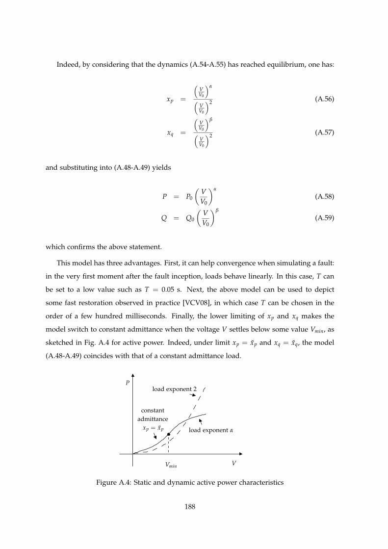
Indeed, by considering that the dynamics (A.54-A.55) has reached equilibrium, one has:
xp =
(VV0
)α
(VV0
)2 (A.56)
xq =
(VV0
)β
(VV0
)2 (A.57)
and substituting into (A.48-A.49) yields
P = P0
(VV0
)α
(A.58)
Q = Q0
(VV0
)β
(A.59)
which confirms the above statement.
This model has three advantages. First, it can help convergence when simulating a fault:
in the very first moment after the fault inception, loads behave linearly. In this case, T can
be set to a low value such as T = 0.05 s. Next, the above model can be used to depict
some fast restoration observed in practice [VCV08], in which case T can be chosen in the
order of a few hundred milliseconds. Finally, the lower limiting of xp and xq makes the
model switch to constant admittance when the voltage V settles below some value Vmin, as
sketched in Fig. A.4 for active power. Indeed, under limit xp = xp and xq = xq, the model
(A.48-A.49) coincides with that of a constant admittance load.
P
VVmin
xp = xp
constantadmittance
load exponent α
load exponent 2
Figure A.4: Static and dynamic active power characteristics
188
It is easily shown that xp and xq relate to Vmin through:
xp =
(Vmin
V0
)α−2
(A.60)
xq =
(Vmin
V0
)β−2
(A.61)
A.3.2 Hybrid part of the model
The bounds on xp and xq are easily transformed into a model of the type (2.12):
(1− z2p)xp = (1− z2
p)
(VV0
)α− xp
(VV0
)2
Tp+ z2
pxp − σ(zp)xp − σ(−zp)xp (A.62)
(1− z2q)xq = (1− z2
q)
(VV0
)β− xq
(VV0
)2
Tq+ z2
qxq − σ(zq)xq − σ(−zq)xq (A.63)
where function σ is equal to 1 if its argument is positive, 0 otherwise. The jump conditions
are:
zp(t+j ) = 1 if zp(t−j ) = 0 and xp > xp
zp(t+j ) = −1 if zp(t−j ) = 0 and xp < xp (A.64)
zp(t+j ) = 0 if zp(t−j ) = ±1 and zp xp < 0
zq(t+j ) = 1 if zq(t−j ) = 0 and xq > xq
zq(t+j ) = −1 if zq(t−j ) = 0 and xq < xq (A.65)
zq(t+j ) = 0 if zq(t−j ) = ±1 and zq xq < 0
where xp is computed from (A.54) and xq from (A.55).
The discrete variables zp and zq take values in the finite set {−1, 0, 1}. Equations (A.62)
and (A.63) can thus be decomposed with simple substitutions into the three flows corre-
sponding to each value in the finite set {−1, 0, 1}.Indeed for zp = 1 it holds:
0 = xp − xp
which simply forces xp to its upper limit xp. For zp = −1, the lower limit xp is enforced. In
a similar way, the upper xq and lower xq limits are enforced on xq.
189

A.3.3 Overall model
The four continuous variables ix, iy, xp, xq and the two discrete variables zp, zq are balanced
by:
• 2 algebraic equations of the type (2.2) (stator equations): (A.52, A.53)
• 2 algebraic-differential equations of the type (2.3, 2.4) (restoration equations) : (A.62,
A.63)
• 2 discrete transition equations of the type (2.5) (jump conditions) : (A.64, A.65)
In fact, the two algebraic-differential equations of the type (2.3, 2.4) are here written in
the compact form (A.62, A.63) thanks to the hybrid equation-based formulation (2.12), that
allows a flow to switch from differential to algebraic and viceversa. An equivalent block-
diagram modelling formulation would not be as straightforward, insofar as a differential-
algebraic switch could modify the incidence matrix of the system possibly leading to an
algebraic loop problem.
190

A.4 Computation of BDF coefficients
The polynomial that interpolates p + 1 points of w may be written in Newton’s form as:
φ(t) = w(tj−p) + w[tj−p, tj−p+1](t− tj−p) + . . . (A.66)
+ w[tj−p, . . . , tj−1, tj](t− tj−p) . . . (t− tj−1)
where the divided differences are defined recursively as:
w(ti) = w[ti] (A.67)
w[ti−k, ti−k+1, . . . , ti−1, ti] =w[ti−k+1, . . . , ti]−w[ti−k, . . . , ti−1]
ti − ti−k(A.68)
The p-order BDF method is obtained by imposing Eq. (3.5), hereafter repeated for cove-
nience:
φ(tj) = w(tj) (A.69)
where tj is the instant where the value of w has to be computed, while its values at the
previous p points are known.
BEM can be easily derived with this procedure, by setting p = 1:
φ(t) = w(tj−1) + w[tj−1, tj](t− tj−1) = w(tj−1) +w(tj)−w(tj−1)
tj − tj−1(t− tj−1) (A.70)
Taking the time derivative of (A.70) and substituting in (A.69) yields:
w(tj) =w(tj)−w(tj−1)
tj − tj−1
The classical BEM formula (3.2) is then obtained by isolating w(tj) and setting h =
tj − tj−1:
w(tj) = w(tj−1) + hw(tj) (A.71)
In order to obtain the BDF2 coefficients, let us consider 3 interpolation points, i.e. p = 2:
φ(t) = w(tj−2) + w[tj−2, tj−1](t− tj−2) + w[tj−2, tj−1, tj](t− tj−2)(t− tj−1) (A.72)
= w(tj−2) +w(tj−1)−w(tj−2)
tj−1 − tj−2(t− tj−2) +
w[tj−1, tj]−w[tj−2, tj−1]
tj − tj−2(t− tj−2)(t− tj−1)
= w(tj−2) +w(tj−1)−w(tj−2)
tj−1 − tj−2(t− tj−2)
+
(w(tj)−w(tj−1)
(tj − tj−1)(tj − tj−2)− w(tj−1)−w(tj−2)
(tj−1 − tj−2)(tj − tj−2)
)(t− tj−2)(t− tj−1)
191

Taking the time derivative of (A.72) yields:
φ(t) =w(tj−1)−w(tj−2)
tj−1 − tj−2(A.73)
+
(w(tj)−w(tj−1)
(tj − tj−1)(tj − tj−2)− w(tj−1)−w(tj−2)
(tj−1 − tj−2)(tj − tj−2)
)(2t− tj−1 − tj−2)
which is then evaluated in tj:
φ(tj) =w(tj−1)−w(tj−2)
tj−1 − tj−2(A.74)
+
(w(tj)−w(tj−1)
(tj − tj−1)(tj − tj−2)− w(tj−1)−w(tj−2)
(tj−1 − tj−2)(tj − tj−2)
)(2tj − tj−1 − tj−2)
Without loss of generality, the notation in (A.74) can be simplified by introducing h =
tj−1 − tj−2 and ξh = tj − tj−1:
φ(tj) =w(tj−1)−w(tj−2)
h+
(w(tj)−w(tj−1)
(ξh)(h + ξh)− w(tj−1)−w(tj−2)
(h)(h + ξh)
)(h + 2ξh)
=w(tj−1)−w(tj−2)
h+
(w(tj)−w(tj−1)
(ξh)(1 + ξ)− w(tj−1)−w(tj−2)
(h)(1 + ξ)
)(1 + 2ξ)
=1h
(w(tj)
1 + 2ξ
ξ(1 + ξ)+ w(tj−1)
(1− 1 + 2ξ + ξ + 2ξ2
ξ(1 + ξ)
)+ w(tj−2)
(1 + 2ξ
1 + ξ− 1))
=1h
(w(tj)
1 + 2ξ
ξ(1 + ξ)−w(tj−1)
1 + 2ξ + ξ2
ξ(1 + ξ)+ w(tj−2)
ξ
1 + ξ
)=
1h
(w(tj)
1 + 2ξ
ξ(1 + ξ)−w(tj−1)
1 + ξ
ξ+ w(tj−2)
ξ
1 + ξ
)(A.75)
By substituting (A.69) into (A.75) we obtain
w(tj) =1h
(w(tj)
1 + 2ξ
ξ(1 + ξ)−w(tj−1)
1 + ξ
ξ+ w(tj−2)
ξ
1 + ξ
)which can be rearranged and fitted to the classical BDF form (3.4) by isolating w(tj):
w(tj) =(1 + ξ)2
1 + 2ξw(tj−1)−
ξ2
1 + 2ξw(tj−2) + h
ξ(1 + ξ)
1 + 2ξw(tj) (A.76)
=2
∑`=1
γ` w(tj−`) + h β w(tj) (A.77)
where
γ1 =(1 + ξ)2
1 + 2ξ(A.78)
γ2 = − ξ2
1 + 2ξ(A.79)
β =ξ(1 + ξ)
1 + 2ξ(A.80)
It can be easily verified that, by imposing ξ = 1, i.e. h = tj−1 − tj−2 = tj − tj−1, the
fixed-step BDF2 coefficients (γ1 = 43 ,γ2 = − 1
3 ,β = 23 ) shown in Table 3.1 are obtained.
192

A.5 Implementation aspects
The program used for the simulation results shown in this thesis, named RAMSES1 has been
developed since 2008, at the University of Liege, jointly by the author and Prof. Thierry Van
Cutsem and, since 2011, with the help of Petros Aristidou. Most of the software is written
in Fortran 95 language.
The partial derivatives relative to network and synchronous machine equations are com-
puted analytically, while those relative to the machine controllers as well as the other injec-
tors are evaluated by finite differences.
In the integrated schemes (I and T), the ma41 sparse solver from Harwell [hsl12] is
used to deal with the system of equations (2.11) and (3.6), considered as a whole. The
Jacobian matrix factorization is dealt with in a dishonest way, following a classical strategy
that consists in updating the Jacobian after major discrete changes (thus excluding LTC
moves, for instance) and in general after E iterations are performed with the same factors
without achieving convergence. E has been set to 3, which has been found to offer a good
compromise between the burden of updating the factors and the burden of performing too
many Newton iterations.
The schemes based on BBD decomposition (A, L and C) use the DGETR BLAS routines
[LHKK79] for dense matrices to deal with the injector systems (4.9) and the ma37 sparse
solver from Harwell [hsl12] to deal with the network system (4.11). The Jacobian matrix
factorization is again dishonest, and different strategies are adopted for the injectors and
for the network. The network matrix is refactorized after major discrete changes (LTC moves
excluded, for instance), and after E iterations are performed with the same factors without
achieving convergence: in this case E is set to a higher value, i.e. 5, than in the integrated
case, because this matrix is almost constant in between topological changes; indeed it would
be constant if it was not for the corrections −CiBi (see Section 4.2). The injector systems
are factorized: (i) after a step size variation, (ii) after a discrete change affecting the specific
injector, and (iii) if the ratio between one injector mismatch (4.9) at iterations k + 1 and k is
higher than a given threshold r at a given iteration. Setting r = 0.75 proved to be a good
compromise.
The CPU times have been measured on a standard laptop with the following character-
istics: Intel Core i7-2630QM CPU, 2.9 GHz, 8 GB RAM, running under Ubuntu Linux 11.04,
1Acronym for “Relaxable Accuracy Multithreaded Simulator of Electric power Systems”.
193

using one core. The code profiling results have been obtained with Intel VTune Amplifier
XE on the same platform, and do not take into account the time spent in data reading and
loading.
194

Bibliography
Ὁ βίος βραχύς, ἡ δὲ τέχνη μακρή 1
[ABJ94] J. Y. Astic, A. Bihain, and M. Jerosolimski. The mixed Adams-BDF variable
step size algorithm to simulate transient and long term phenomena in power
systems. IEEE Trans. Power Syst., 9(2):929–935, May 1994. 50, 124
[ANL+12] U. D. Annakkage, N. K. C. Nair, Y. Liang, A. M. Gole, V. Dinavahi, B. Gus-
tavsen, T. Noda, H. Ghasemi, A. Monti, M. Matar, R. Iravani, and J. A. Mar-
tinez. Dynamic System Equivalents: A Survey of Available Techniques. IEEE
Trans. Power Delivery, 27(1):411–420, Jan. 2012. 96
[AP98] U. M. Ascher and L. R. Petzold. Computer methods for ordinary differential equa-
tions and differential-algebraic equations. Miscellaneous Titles in Applied Math-
ematics Series. Society for Industrial and Applied Mathematics, 1998. 22, 23,
26, 42, 44, 46, 124
[AST83] O. Alsac, B. Stott, and W. F. Tinney. Sparsity-Oriented Compensation Methods
for Modified Network Solutions. IEEE Trans. Power Apparatus and Systems,
PAS-102(5):1050–1060, May 1983. 601The lyf so short, the craft so long to lerne [sic]. Hippocrates of Cos in Aphorisms. Also known in its Latin form
ars longa, vita brevis. Free translation in Middle English by Geoffrey Chaucer in The Parliament of Fowles.
195
[BET91] R. Bacher, G. C. Ejebe, and W. F. Tinney. Approximate sparse vector techniques
for power network solutions. IEEE Trans. Power Syst., 6(1):420–428, Feb. 1991.
22, 96
[BGH72] R. K. Brayton, F. G. Gustavson, and G. D. Hachtel. A new efficient algorithm
for solving differential-algebraic systems using implicit backward differentia-
tion formulas. Proceedings of the IEEE, 60(1):98–108, Jan. 1972. 43
[BL89] V. Brandwajn and M. G. Lauby. Complete bounding method for AC contin-
gency screening. IEEE Trans. Power Syst., 4(2):724–729, May 1989. 96
[Boe77] Boeing Computer Services, Inc. Power System Dynamic Analysis Phase I. EPRI
EL-484 Project 670-1, Final report. EPRI, 1977. 21, 58
[Bos03] A. Bose. Power System Stability: New Opportunities for Control. Book Chapter
in Stability and Control of Dynamical Systems and Applications, D. Liu and P. J.
Antsaklis, Editors. Birkhauser, 2003. 57
[Bra88] V. Brandwajn. Efficient bounding method for linear contingency analysis.
IEEE Trans. Power Syst., 3(1):38–43, Feb. 1988. 96
[Bra93] V. Brandwajn. Localization Concepts in (In)-Security Analysis. In Proc. 1993
Athens Power Tech Conf., volume 1, pages 10–15, Sept. 1993. 22, 95
[BT89] R. Bacher and W. F. Tinney. Faster local power flow solutions: the zero mis-
match approach. IEEE Trans. Power Syst., 4(4):1345–1354, Nov. 1989. 22, 96
[BTS96] S. Bernard, G. Trudel, and G. Scott. A 735 kV shunt reactors automatic switch-
ing system for Hydro-Quebec network. IEEE Trans. Power Syst., 11(4):2024–
2030, Nov. 1996. 35
[BW98] D. Baraff and A. Witkin. Large steps in cloth simulation. In Proc. 25th annual
conference on Computer graphics and interactive techniques, SIGGRAPH ’98, pages
43–54, New York, NY, USA, 1998. ACM. 22, 125
[CB86] S. M. Chan and V. Brandwajn. Partial Matrix Refactorization. IEEE Trans.
Power Syst., 1(1):193–199, Feb. 1986. 60
196
[CC94] M. L. Crow and J. G. Chen. The multirate method for simulation of power
system dynamics. IEEE Trans. Power Syst., 9(3):1684–1690, Aug. 1994. 20, 59
[CC96] M. L. Crow and J. G. Chen. The multirate simulation of FACTS devices in
power system dynamics. IEEE Trans. Power Syst., 11(1):376–382, Feb. 1996. 59
[CC08] J. Chen and M. L. Crow. A variable partitioning strategy for the multirate
method in power systems. IEEE Trans. Power Syst., 23(2):259–266, May 2008.
22, 59, 97, 123
[Cho82] J. H. Chow. Time-scale modeling of dynamic networks with applications to power
systems. Lecture notes in control and information sciences. Springer-Verlag,
1982. 96
[CI90] M. L. Crow and M. Ilic. The parallel implementation of the waveform re-
laxation method for transient stability simulations. IEEE Trans. Power Syst.,
5(3):922–932, Aug. 1990. 59
[CK06] F. E. Cellier and E. Kofman. Continuous system simulation. Springer, 2006. 22,
26, 27, 28, 31, 44, 49, 50, 52, 124, 186
[CZBT91] J. S. Chai, N. Zhu, A. Bose, and D. J. Tylavsky. Parallel Newton type methods
for power system stability analysis using local and shared memory multipro-
cessors. IEEE Trans. Power Syst., 6(4):1539–1545, Nov 1991. 20
[DS72] H. W. Dommel and N. Sato. Fast Transient Stability Soultions. IEEE Trans.
Power Apparatus and Systems, PAS-91(4):1643–1650, July 1972. 46
[EFV07] A. Efrat, Q. Fan, and S. Venkatasubramanian. Curve Matching, Time Warping,
and Light Fields: New Algorithms for Computing Similarity between Curves.
Journal of Mathematical Imaging and Vision, 27(3):203–216, Apr. 2007. 54
[EPT92] G. C. Ejebe, R. F. Paliza, and W. F. Tinney. An adaptive localization method
for real-time security analysis. IEEE Trans. Power Syst., 7(2):777–783, May 1992.
22, 96
[FCPVC11] D. Fabozzi, A. S. Chieh, P. Panciatici, and T. Van Cutsem. On simplified
handling of state events in time-domain simulation. In Proc. 17th Power System
Computation Conference (PSCC), pages 1–9, Aug. 2011. 23, 24, 126, 128
197

[FGWVC09] D. Fabozzi, M. Glavic, L. Wehenkel, and T. Van Cutsem. Security assessment
by multiple transmission system operators exchanging sensitivity and tie-line
power flow information. In Proc. 2009 IEEE Bucharest PowerTech conf., pages 1
–8, June 2009. 96
[FMT12] C. Fu, J. D. McCalley, and J. Tong. A numerical solver design for extended-
term time-domain simulation. IEEE Trans. Power Syst., 2012. IEEE Early Ac-
cess. 50
[FP78] J. Fong and C. Pottle. Parallel Processing of Power System Analysis Problems
Via Simple Parallel Microcomputer Structures. IEEE Trans. Power Apparatus
and Systems, PAS-97(5):1834–1841, Sept. 1978. 58
[FVC09] D. Fabozzi and T. Van Cutsem. Simplified time-domain simulation of detailed
long-term dynamic models. In Proc. 2009 IEEE PES General Meeting, pages 1–8,
July 2009. 22, 23, 24, 49, 124, 125, 129, 130, 180
[FVC10] D. Fabozzi and T. Van Cutsem. Localization and latency concepts applied
to time simulation of large power systems. In Proc. 2010 Bulk Power System
Dynamics and Control - VIII IREP Symposium, pages 1–14, Aug. 2010. 24, 101
[FVC11a] D. Fabozzi and T. Van Cutsem. Assessing the proximity of time evolutions
through dynamic time warping. IET Generation, Transmission & Distribution,
5(12):1268–1276, Dec. 2011. 24, 54, 56
[FVC11b] D. Fabozzi and T. Van Cutsem. On angle references in long-term time-domain
simulations. IEEE Trans. Power Syst., 26(1):483–484, Feb. 2011. 24, 28, 177
[FX06] D. Z. Fang and Y. Xiaodong. A new method for fast dynamic simulation of
power systems. IEEE Trans. Power Syst., 21(2):619–628, May 2006. 59
[Gal84] F. D. Galiana. Bound Estimates of the Severity of Line Outages in Power
System Contingency Analysis and Ranking. IEEE Trans. Power Apparatus and
Systems, PAS-103(9):2612–2624, Sept. 1984. 96
[gC07] CIGRE Working group C4.601. Review of On-line Dynamic Security Assessment
Tools and Techniques. Technical Brochure 325. CIGRE, 2007. 20
198
[GCA+00] S. Gissinger, P. Chaumes, J.-P. Antoine, A. Bihain, and M. Stubbe. Advanced
dispatcher training simulator. Computer Applications in Power, IEEE, 13(2):25–
30, Apr. 2000. 175
[Gea71] C. W. Gear. Numerical initial value problems in ordinary differential equations.
Prentice-Hall series in automatic computation. Prentice-Hall, 1971. 43, 49, 129
[GLVC05] M. E. Grenier, D. Lefebvre, and T. Van Cutsem. Quasi steady-state models
for long-term voltage and frequency dynamics simulation. In Power Tech, 2005
IEEE Russia, pages 1–8, June 2005. 122
[GP78] A. J. Germond and R. Podmore. Dynamic Aggregation of Generating Unit
Models. IEEE Trans. Power Apparatus and Systems, PAS-97(4):1060–1069, July
1978. 96
[HB28] E. Hubbard and F. Bann. Little Journeys to the Homes of the Great, volume 1.
W.H. Wise & Co., 1928. 173
[HBJVN77] W. L. Hatcher, F. M. Brasch Jr., and J. E. Van Ness. A feasibility study for
the solution of transient stability problems by multiprocessor structures. IEEE
Trans. Power Apparatus and Systems, 96(6):1789–1797, Nov. 1977. 21, 58
[HP00] I. A. Hiskens and M. A. Pai. Trajectory sensitivity analysis of hybrid sys-
tems. IEEE Trans. Circuits and Systems I: Fundamental Theory and Applications,
47(2):204–220, Feb. 2000. 27, 30, 126
[hsl12] HSL. A collection of Fortran codes for large scale scientific computation.
http://www.hsl.rl.ac.uk. accessed May 2012. 193
[HSV81] G. D. Hachtel and A. L. Sangiovanni-Vincentelli. A survey of third-generation
simulation techniques. Proceedings of the IEEE, 69(10):1264–1280, Oct. 1981. 22,
95
[IEE92] IEEE Task Force of Power System Engineering Committee. Parallel processing
in power systems computation. IEEE Trans. Power Syst., 7(2):629–638, May
1992. 47
199

[ISCP87] M. Ilic’-Spong, M. L. Crow, and M. A. Pai. Transient Stability Simulation by
Waveform Relaxation Methods. IEEE Trans. Power Syst., 2(4):943–949, Nov.
1987. 20, 59
[JMD09] V. Jalili-Marandi and V. Dinavahi. Instantaneous Relaxation-Based Real-Time
Transient Stability Simulation. IEEE Trans. Power Syst., 24(3):1327–1336, Aug.
2009. 20, 59
[JMD10] V. Jalili-Marandi and V. Dinavahi. SIMD-Based Large-Scale Transient Sta-
bility Simulation on the Graphics Processing Unit. IEEE Trans. Power Syst.,
25(3):1589–1599, Aug. 2010. 20
[KL10] Y. Kong and S. Liu. Power system transient stability assessment based on
geometric features of disturbed trajectory and DTW. In Proc. 6th International
Conference on Natural Computation (ICNC 2010), pages 485–489, Aug. 2010. 54
[KMC08] S. K. Khaitan, J. D. McCalley, and Q. Chen. Multifrontal Solver for Online
Power System Time-Domain Simulation. IEEE Trans. Power Syst., 23(4):1727–
1737, Nov. 2008. 21
[KOO+93] A. Kurita, H. Okubo, K. Oki, S. Agematsu, D. B. Klapper, N. W. Miller, W. W.
Price Jr., J. J. Sanchez-Gasca, K. A. Wirgau, and T. D. Younkins. Multiple time-
scale power system dynamic simulation. IEEE Trans. Power Syst., 8(1):216–223,
Feb. 1993. 23, 150
[KP01] E. J. Keogh and M. J. Pazzani. Derivative Dynamic Time Warping. In First
SIAM International Conference on Data Mining (SDM’2001, pages 1–11, Apr.
2001. 54
[Kun94] P. Kundur. Power system stability and control. The EPRI power system engineer-
ing series. McGraw-Hill, 1994. 19, 21, 27
[Lar04] M. Larsson. ObjectStab-an educational tool for power system stability studies.
IEEE Trans. Power Syst., 19(1):56–63, Feb. 2004. 28
[LHKK79] C. L. Lawson, R. J. Hanson, D. R. Kincaid, and F. T. Krogh. Basic Linear
Algebra Subprograms for Fortran Usage. ACM Trans. Math. Softw., 5(3):308–
323, Sept. 1979. 193
200

[LRLVC01] L. Loud, P. Rousseaux, D. Lefebvre, and T. Van Cutsem. A time-scale
decomposition-based simulation tool for voltage stability analysis. In Power
Tech Proceedings, 2001 IEEE Porto, volume 2, page 6 pp. vol.2, Sept. 2001. 151
[LSBTC90] M. La Scala, A. Bose, D. J. Tylavsky, and J. S. Chai. A highly parallel method
for transient stability analysis. IEEE Trans. Power Syst., 5(4):1439–1446, Nov.
1990. 20, 59
[LSBTT90] M. La Scala, M. Brucoli, F. Torelli, and M. Trovato. A Gauss-Jacobi-Block-
Newton method for parallel transient stability analysis [of power systems].
IEEE Trans. Power Syst., 5(4):1168–1177, Nov. 1990. 59
[Lyg04] J. Lygeros. Lecture Notes on Hybrid Systems. ENSIETA 2-6/2/2004. Department
of Electrical and Computer Engineering, University of Patras, 2004. 31, 49
[MDGS79] A. Monticelli, S. Deckmann, A. Garcia, and B. Stott. Real-Time External Equiv-
alents for Static Security Analysis. IEEE Trans. Power Apparatus and Systems,
PAS-98(2):498–508, Mar. 1979. 96
[MFL+05] A. Monti, H. Figueroa, S. Lentijo, X. Wu, and R. Dougal. Interface Issues
in Hardware-in-the-Loop Simulation. In Electric Ship Technologies Symposium,
2005 IEEE, pages 39–45, July 2005. 128
[Mil12] F. Milano. Extraneous instabilities arising in power systems with non-
synchronous distributed energy resources. International Journal of Electrical
Power & Energy Systems, 34(1):174–176, 2012. 27
[ML89] J. R. Marti and J. Lin. Suppression of numerical oscillations in the EMTP
power systems. IEEE Trans. Power Syst., 4(2):739–747, May 1989. 23, 125
[MR06] F. Magoules and F.-X. Roux. Lagrangian formulation of domain decomposi-
tion methods: A unified theory. Applied Mathematical Modelling, 30(7):593–615,
2006. 20, 59
[Nor61] A. Nordsieck. On numerical integration of ordinary differential equations. Univ. of
Illinois, Coordinated Science Laboratory, 1961. 43
[Ogr94] J. Ogrodzki. Circuit simulation methods and algorithms. Electronic engineering
systems series. CRC Press, 1994. 21, 58
201

[PC11] P. Panciatici and A. S. Chieh. Equation-based hybrid modeling of power sys-
tems for time-domain simulation. In Proc. 2011 IEEE PES General Meeting,
pages 1–9, July 2011. 29
[PCLG+11] F. Pruvost, T. Cadeau, P. Laurent-Gengoux, F. Magoules, F.-X. Bouchez, and
B. Haut. Numerical accelerations for power systems transient stability simu-
lations. In Proc. 17th Power System Computation Conference (PSCC), pages 1–8,
Aug. 2011. 20
[peg12] PEGASE project. http://www.fp7-pegase.eu. accessed May 2012. 37
[RBFEVC12] R. Ramırez-Betancour, C. R. Fuerte-Esquivel, and T. Van Cutsem. A two-time
scale simulation for dynamic analysis of power systems. Electric Power Systems
Research, 83(1):185–195, 2012. 151
[RM09] J. Rommes and N. Martins. Exploiting structure in large-scale electrical circuit
and power system problems. Linear Algebra and its Applications, 431(3-4):318–
333, 2009. Special Issue in honor of Henk van der Vorst. 58
[RSVH79] N. B. G. Rabbat, A. L. Sangiovanni-Vincentelli, and H. Y. Hsieh. A multilevel
Newton algorithm with macromodeling and latency for the analysis of large-
scale nonlinear circuits in the time domain. IEEE Trans. on Circuits and Systems,
26(9):733–741, Sept. 1979. 97
[SBDB89] M. Stubbe, A. Bihain, J. Deuse, and J. C. Baader. STAG-a new unified software
program for the study of the dynamic behaviour of electrical power systems.
IEEE Trans. Power Syst., 4(1):129–138, Feb. 1989. 175, 178
[SC78] H. Sakoe and S. Chiba. Dynamic programming algorithm optimization for
spoken word recognition. IEEE Trans. on Acoustics, Speech, and Signal Process-
ing, 26(1):43–49, Feb. 1978. 54, 55
[SGDPP95] J.J. Sanchez-Gasca, R. D’Aquila, W.W. Price, and J.J. Paserba. Variable time
step, implicit integration for extended-term power system dynamic simula-
tion. In Power Industry Computer Application Conference, 1995 IEEE, pages 183–
189, May 1995. 50
202
[SLM+00] K. Strunz, L. Linares, J. R. Marti, O. Huet, and X. Lombard. Efficient and accu-
rate representation of asynchronous network structure changing phenomena
in digital real time simulators. IEEE Trans. Power Syst., 15(2):586–592, May
2000. 128
[Sto79] B. Stott. Power system dynamic response calculations. Proceedings of the IEEE,
67(2):219–241, Feb. 1979. 49
[Str04] K. Strunz. Flexible Numerical Integration for Efficient Representation of
Switching in Real Time Electromagnetic Transients Simulation. IEEE Trans.
on Power Delivery, 19(3):1276–1283, July 2004. 128
[Stu95] M. Stubbe. Long-Term Dynamics - Phase II. Report of CIGRE Task Force
38.02.08, Jan. 1995. 32
[SVM07] J. A. Sanders, F. Verhulst, and J. A. Murdock. Averaging methods in nonlinear
dynamical systems. Applied mathematical sciences. Springer, 2007. 22, 123
[TBC85] W. F. Tinney, V. Brandwajn, and S. M. Chan. Sparse Vector Methods. IEEE
Trans. Power Apparatus and Systems, PAS-104(2):295–301, Feb. 1985. 22, 96
[TBS99] G. Trudel, S. Bernard, and G. Scott. Hydro-Quebec’s defence plan against
extreme contingencies. IEEE Trans. Power Syst., 14(3):958–966, Aug. 1999. 35
[TGQS09] P. Tormene, T. Giorgino, S. Quaglini, and M. Stefanelli. Matching incomplete
time series with dynamic time warping: an algorithm and an application to
post-stroke rehabilitation. Artificial Intelligence in Medicine, 45(1):11–34, Jan.
2009. 54
[Tin79] W. F. Tinney. This Week’s Citation Classics, 18:30, Apr. 1979. 5
[TS72] C. J. Tavora and O. J. M. Smith. Characterization of Equilibrium and Stability
in Power Systems. IEEE Trans. Power Apparatus and Systems, PAS-91(3):1127–
1130, May 1972. 27, 178
[TW67] W. F. Tinney and J. W. Walker. Direct solutions of sparse network equations by
optimally ordered triangular factorization. Proceedings of the IEEE, 55(11):1801–
1809, Nov. 1967. 46
203
[TW05] A. Toselli and O. B. Widlund. Domain Decomposition Methods - Algorithms and
Theory. Springer series in computational mathematics. Springer, 2005. 97
[VCGL06] T. Van Cutsem, M. E. Grenier, and D. Lefebvre. Combined detailed and quasi
steady-state time simulations for large-disturbance analysis. International Jour-
nal of Electrical Power & Energy Systems, 28(9):634–642, 2006. Selection of Papers
from 15th Power Systems Computation Conference, 2005. 151
[VCJMP95] T. Van Cutsem, Y. Jacquemart, J. N. Marquet, and P. Pruvot. A comprehensive
analysis of mid-term voltage stability. IEEE Trans. Power Syst., 10(3):1173–1182,
Aug. 1995. 122
[VCM97] T. Van Cutsem and R. Mailhot. Validation of a fast voltage stability analysis
method on the Hydro-Quebec system. IEEE Trans. Power Syst., 12(1):282–292,
Feb. 1997. 122
[VCV08] T. Van Cutsem and C. Vournas. Voltage Stability of Electric Power Systems. Power
Electronics and Power Systems. Springer, 2008. 21, 122, 135, 187, 188
[Vin68] T. K. Vintsyuk. Speech discrimination by dynamic programming. Cybernetics,
4(1):52–57, 1968. Russian Kibernetika 4(1):81-88 (1968). 54, 55
[VVC06] C. Vournas and T. Van Cutsem. On-line voltage security assessment. In Real-
time stability in power systems, pages 119–146. Springer, 2006. 175
[War49] J. B. Ward. Equivalent Circuits for Power-Flow Studies. Transactions of the
American Institute of Electrical Engineers, 68(1):373–382, July 1949. 95
[WC11] K. Wang and M. L. Crow. Numerical simulation of Stochastic Differential
Algebraic Equations for power system transient stability with random loads.
In Proc. 2011 IEEE PES General Meeting, pages 1–8, July 2011. 22, 124
[WM83] F. F. Wu and A. Monticelli. Critical review of external network modelling
for online security analysis. International Journal of Electrical Power & Energy
Systems, 5(4):222–235, Oct. 1983. Special Issue Control Centres. 96
[YAGESS04] A. M. Youssef, T. K. Abdel-Galil, E. F. El-Saadany, and M. M. A. Salama. Dis-
turbance classification utilizing dynamic time warping classifier. IEEE Trans.
on Power Delivery, 19(1):272 – 278, Jan. 2004. 54
204

[YES81] Y. Yu and M. A. El-Sharkawi. Estimation of External Dynamic Equivalents
of a Thirteen-Machine System. IEEE Trans. Power Apparatus and Systems, PAS-
100(3):1324–1332, Mar. 1981. 96
[ZA05] Y. Zhou and V. Ajjarapu. A novel approach to trace time-domain trajectories of
power systems in multiple time scales. IEEE Trans. Power Syst., 20(1):149–155,
Feb. 2005. 151
[Zha05] F. Zhang. The Schur complement and its applications. Numerical methods and
algorithms. Springer Science, 2005. 21, 63
[ZWP80] J. Zaborszky, K.-W. Whang, and K. Prasad. Fast Contingency Evaluation Using
Concentric Relaxation. IEEE Trans. Power Apparatus and Systems, PAS-99(1):28–
36, Jan. 1980. 96
205

.