a simple quality triangulation algorithm for complex geometries

INTERNATIONAL JOURNAL FOR NUMERICAL METHODS IN FLUIDSInt. J. Numer. Meth. Fluids 2011; 66:1447–1464Published online 30 March 2010 in Wiley Online Library (wileyonlinelibrary.com). DOI: 10.1002/fld.2323

A simple quality triangulation algorithm for complex geometries

Yaoxin Zhang∗,†,‡, Yafei Jia§ , H. C. Chan¶ and Sam S. Y. Wang‖

National Center for Computational Hydroscience and Engineering, The University of Mississippi,102 Carrier Hall, University, MS 38677, U.S.A.

SUMMARY

This paper presents a simple algorithm for quality triangulation in domains with complex geometries.Based on the fact that the equilateral triangles (regular meshes) are ideal for numerical computations incomputational fluids dynamics (CFD) analysis, the proposed algorithm starts with an initial equilateraltriangle mesh covering the whole domain. Nodes close to the boundary edges satisfy the so-called non-encroaching criterion, the distance from any inserted node to any boundary vertices and the midpointsof any boundary edge is greater than a given characteristic length. Both nearly uniform and non-uniformtriangle meshes can be generated using a mesh size reduction technique. Local refinement is achievedby using transition layers. More regular meshes can be generated in the interior of the domain and allangles of the triangle mesh produced by this algorithm are proven to be bounded in a reasonable range(19.5–141◦). Copyright q 2010 John Wiley & Sons, Ltd.

Received 21 October 2009; Revised 14 January 2010; Accepted 16 February 2010

KEY WORDS: triangulation; Delaunay; refinement

1. INTRODUCTION

Triangle meshes are widely used in computational fluids dynamics (CFD) to help solve a set ofhighly non-linear partial differential equations (PDE). They are more suitable for conforming to thecomplex domain geometries and setting adequate local resolutions, which still remain a challengein quality structured mesh generation. Triangle mesh generation is desired not only in CFDanalysis, but also in many other disciplines, such as computer-aided design, computer graphics, andglobal information system (GIS), etc. A ‘good-quality’ triangle mesh usually refers to those withwell-shaped triangles, no small angles (a ‘small’ angle is usually quantified by a bound) excludingthe input small angles formed by the boundary edges, or/and, no obtuse angles. Other criteriainclude the density control (adaptivity) and optimal size (number of triangles), etc.

Two major triangulation methods have been successfully developed and applied, Delaunaytriangulation method (DTM) [1–9] and advancing front method (AFM) [10]. DTM is based on theempty-circle criterion that no point is interior to the circumcircle of any triangle, whereas AFM

∗Correspondence to: Yaoxin Zhang, National Center for Computational Hydroscience and Engineering, The Universityof Mississippi, 102 Carrier Hall, University, MS 38677, U.S.A.

†E-mail: [email protected]‡Research Scientist.§Research Professor and Associate Director.¶Post-Doctoral Research Associate.‖F.A.P Barnard Distinguished Professor and Director.

Contract/grant sponsor: USDA Agriculture Research Service; contract/grant number: 58-6408-2-0062Contract/grant sponsor: Department of Homeland Security-sponsored Southeast Region Research Initiative (SERRI)

Copyright q 2010 John Wiley & Sons, Ltd.

1448 Y. ZHANG ET AL.

uses marching techniques to advance front cell faces from boundaries to interior domain. Thepresent work falls into the category of the DTM.

To further improve speed and quality of Delaunay triangulation (DT), many algorithms andmethodologies have been developed. The famous Bowyer–Watson algorithm was proposed byBowyer [2] and Watson [9] independently at the same time in 1981 for computing the Voronoidiagram based on a set of points in n-dimensions. In 1985, Guibas and Stolfi [6] proposed a divide-and-conquer algorithm for efficiently triangulating a set of arbitrary planar points based on a quad-treedata structure, whereas Fortune [5] developed a sweep line algorithm to achieve fast triangulation.

Quality DT for complex domains usually requires a refinement algorithm where points (Steinerpoints) are successively inserted into the domain. Chew [3, 4] first proposed two provably goodDelaunay refinement algorithms for planes and curved surfaces. Ruppert [7] also developed asimilar algorithm and theoretically proved its capability of generating both well-shaped and size-optimal triangle meshes. Both Chew’s and Ruppert’s algorithm iteratively update the triangula-tion by inserting circumcenters of skinny triangles and conditionally splitting boundary edges.Shewchuk [8] analyzed Chew’s second algorithm [4] and Ruppert’s algorithm [7]. Improvementswere made on generating meshes in non-manifold domains with small angles. A popular meshgenerator—Triangle was developed, which is widely used. In 1994, Bern et al. [1] proposed a morecomplicated quadtree refinement algorithm with no small and obtuse angles and size (number ofelements) controlled.

In this study, a simple algorithm for quality triangulation is proposed. Instead of introducingSteiner points into the domain one by one, this triangulation procedure starts with a uniformmesh consists of equilateral triangles. The non-encroaching criterion [7] is used to make themesh conform to complex boundaries. The size reduction process makes this algorithm capableof generating the non-uniform meshes with varied densities as well. The proposed algorithm iscapable of generating regular meshes in the interior of the domain, which is desired by mostnumerical methods in CFD problems especially for transient problems. For example, the detachedboundary layer simulations are no longer so closely tied to the boundary and are preferred toregular meshes away from boundaries.

2. TRIANGULATION ALGORITHM

2.1. Basic concepts

In two-dimension problems, a triangulation usually begins with a planar straight line graph (PSLG)which represents the computational domain and is composed of dangling edges and isolated points.The so-called constrained Delaunay triangulation (CDT) is developed by adding constraints to DTso that all edges and isolated points in PSLG must be included into the triangulation. The word‘encroach’ was first used by Ruppert [7]: a boundary edge is encroached upon by a non-boundaryvertex if it is in the interior of the diametral circle of this edge. The encroached edge will be splitand the encroaching vertex will be removed. This concept was also adopted by other researchers,i.e. in References [4, 8].

In Chew’s second refinement algorithm [4] and Ruppert’s refinement algorithm [7], the circum-center of a skinny triangle is selected to be inserted into the domain due to the observation thatthe smallest angle � of a triangle, T, is half of the angle �(=2�) at the circumcenter and oppositeto the smallest edge (Figure 1).

Chew’s second algorithm [4] removes a skinny triangle with the largest circum circle by insertingits circumcenter cmax into the CDT or splitting the encroached boundary edge and updating theCDT iteratively. There are three basic operations, (1) insert the cmax (free vertex); (2) split theencroached boundary edge; and, (3) remove the encroaching free vertices. The vertex cmax isinserted if it is within the domain and not encroaching any boundary edge; and, a boundary edgeis split if it is encroached by free vertices, and all encroaching free vertices will be removed.

Ruppert’s algorithm [7] is similar to Chew’s second algorithm, but it starts with the DT of theinput PSLG and a rectangle bounding box, which covers the entire PSLG. In Ruppert’s algorithm,

Copyright q 2010 John Wiley & Sons, Ltd. Int. J. Numer. Meth. Fluids 2011; 66:1447–1464DOI: 10.1002/fld

A SIMPLE QUALITY TRIANGULATION ALGORITHM FOR COMPLEX GEOMETRIES 1449

T

αβ

c

(β = 2α)

Figure 1. Circumcenter of skinny triangle as Steiner point.

the non-encroaching circumcenters of all skinny triangles are inserted into the box and all theencroached boundary edges are split successively to improve the mesh quality and ensure that allinput boundary edges are included in the DT.

Both algorithms can produce well-shaped and size-controlled triangle meshes, and Chew’ssecond algorithm [4] basically produces fewer triangles in practice. However, both algorithms aredriven only by grading functions, and there is no control on the distribution of the vertices in thedomain. A typical example of this problem is that both algorithms may not be able to produce thedesired symmetric or nearly symmetric meshes in a symmetric computational domain.

2.2. Current study

In this study, a simple quality triangulation algorithm is proposed. This approach falls into thecategory of the so-called ‘Steiner Triangulation’ which allows the Steiner points in addition tothe points contained in the original PSLG. In References [3, 4, 7, 8], the Steiner points are mainlydefined as the circumcenters of the skinny triangles and the midpoints of the boundary edges,whereas in Reference [1] the points introduced by quadtrees are used. Inspired by an intuitive ideathat the equilateral triangles are ideal elements for computations, a simple algorithm is developedwhich begins with an initial mesh of equilateral triangles covering the whole domain. The boundarytreatment and the size reduction process will make the resulting meshes non-uniform and conform tothe complex boundaries. The proposed algorithm is described as followswith an illustrative example.

Step 1: Refinement of boundaries: The boundary edges of a PSLG except the isolated pointsare refined so that the length of any resultant boundary edge e satisfies the following refinementcondition: emin�e<2emin (refinement condition), where emin can be the length of the shortestboundary edge, the minimum distance between vertices or some user-specified length, and isreferred to as the characteristic length hereafter. A boundary edge splits at its midpoint only if itslength is greater than 2emin. The refinement is an iteration process listed below:

1. Find or specify the characteristic length emin.2. Search through all boundary edges of the PSLG and split them at the midpoints if their length

are greater than 2emin.3. Check whether all boundary edges satisfy the refinement condition. If not, go back to step (2).

The boundary refinement process enforces the refinement condition and ensures that the char-acteristic length emin will not be changed after refinement. This boundary refinement is necessaryfor generating the initial mesh of equilateral triangles and ensuring the quality of the resultingmesh.

Figure 2 shows an example of a PSLG which consists of one outer boundary, one island (hole),two-open polylines, and six-isolated points.

Step 2: Generation of equilateral triangle mesh: An equilateral triangle mesh (ETM) is generatedin a superequilateral triangle (ST) which is required to cover the whole domain, and the edge lengthof each equilateral triangle of the ETM is equal to the characteristic length emin. The diameterof the inner circle of ST is equal to the diagonal of the minimum bounding box of the domain.As shown in Figure 3, there are four types of constructions considered in this study (a) one of its



Figure 2. Input PSLG.

I

J

ST

(a)

IJ

ST

(b)

(c) (d)

I

J

ST

IJ

ST

Figure 3. Four types of supertriangle: (a) altitude is collinear with the left diagonal of the bounding box;(b) altitude is collinear with the right diagonal of the bounding box; (c) altitude is in the direction of

x-axis; and (d) altitude is in the direction of y-axis.



altitudes of the ST is collinear with the left diagonal of the bounding box (Figure 3(a)); (b) one ofits altitudes of the ST is collinear with the right diagonal of the bounding box (Figure 3(b)); (c) oneof its altitudes is in the direction of the x-axis (Figure 3(c)); and (d) one of its altitudes is in thedirection of the y-axis (Figure 3(d)). As three sets of lines parallel to the three edges of the STare used to generate the ETM, it is easily observed that the mesh lines of the ETM generatedin the ST are aligned in three different directions, and the difference between any two directionsis 60◦. Any rotation of the ST for 60◦ will result in an identical ETM with mesh lines aligned tothe same three directions. Other ways of constructing ST based on its inner circle may also beconsidered. For example, in order to generate a symmetric or nearly symmetric triangulation, thesymmetric axis of the symmetric domain must be parallel to the altitude of the ST.

Each vertex in the ETM can be organized in a similar way to the structured mesh and identifiedusing the (I, J ) index. In Figure 3, J is in the direction of the altitude, whereas I is along one edgeof the ST. They are perpendicular to each other. Along the J direction, the mesh lines are uniformlydistributed, and on the J th mesh line there are J number of vertices. This index organization isvery important for the size reduction process.

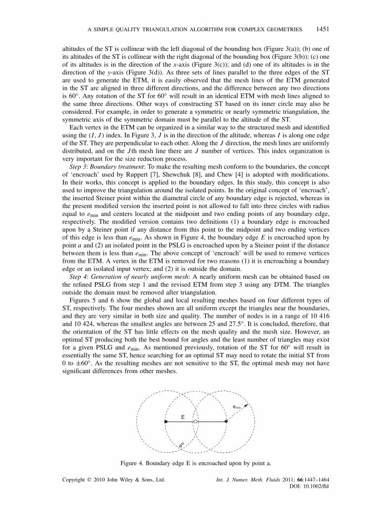
Step 3: Boundary treatment: To make the resulting mesh conform to the boundaries, the conceptof ‘encroach’ used by Ruppert [7], Shewchuk [8], and Chew [4] is adopted with modifications.In their works, this concept is applied to the boundary edges. In this study, this concept is alsoused to improve the triangulation around the isolated points. In the original concept of ‘encroach’,the inserted Steiner point within the diametral circle of any boundary edge is rejected, whereas inthe present modified version the inserted point is not allowed to fall into three circles with radiusequal to emin and centers located at the midpoint and two ending points of any boundary edge,respectively. The modified version contains two definitions (1) a boundary edge is encroachedupon by a Steiner point if any distance from this point to the midpoint and two ending verticesof this edge is less than emin. As shown in Figure 4, the boundary edge E is encroached upon bypoint a and (2) an isolated point in the PSLG is encroached upon by a Steiner point if the distancebetween them is less than emin. The above concept of ‘encroach’ will be used to remove verticesfrom the ETM. A vertex in the ETM is removed for two reasons (1) it is encroaching a boundaryedge or an isolated input vertex; and (2) it is outside the domain.

Step 4: Generation of nearly uniform mesh: A nearly uniform mesh can be obtained based onthe refined PSLG from step 1 and the revised ETM from step 3 using any DTM. The trianglesoutside the domain must be removed after triangulation.

Figures 5 and 6 show the global and local resulting meshes based on four different types ofST, respectively. The four meshes shown are all uniform except the triangles near the boundaries,and they are very similar in both size and quality. The number of nodes is in a range of 10 416and 10 424, whereas the smallest angles are between 25 and 27.5◦. It is concluded, therefore, thatthe orientation of the ST has little effects on the mesh quality and the mesh size. However, anoptimal ST producing both the best bound for angles and the least number of triangles may existfor a given PSLG and emin. As mentioned previously, rotation of the ST for 60◦ will result inessentially the same ST, hence searching for an optimal ST may need to rotate the initial ST from0 to ±60◦. As the resulting meshes are not sensitive to the ST, the optimal mesh may not havesignificant differences from other meshes.

emin

a

E

Figure 4. Boundary edge E is encroached upon by point a.



Figure 5. Nearly uniform mesh for: (a) 10420 nodes and 20388 triangles generated from ST of type A.The smallest angle is 25◦. The other cases b, c, and d are simply listed; (b) 10424 nodes and 20396triangles generated from ST of type B. The smallest angle is 26◦; (c) 10416 nodes and 20380 trianglesgenerated from ST of type C. The smallest angle is 25.9◦; and (d) 10420 nodes and 20388 triangles

generated from ST of type D. The smallest angle is 27.5◦.

Lemma 1The nearly uniform triangulation obtained from step 1 to 4 includes the entire PSLG.

ProofA PSLG can include open or closed polylines and isolated points, if no edges in the PSLG arecrossed and no isolated points are removed, the triangulation will include the entire PSLG. Thus,there are basically three cases (1) for the outer boundary and the islands (holes) (they are closedpolylines), because there are no vertices outside of domain, no edge of free vertices will crosstheir edges; (2) For the isolated points, since they are not removed, they will be included into thetriangulation as well; and, (3) As for the dangling edges (open polylines) inside the domain, ifone such edge ec is crossed by another edge es , according to the empty-circle criterion, es mustbe shorter than ec. A worst scenario of such a case is shown in Figure 7 where a dangling edgeec (e1e2) is assumed crossed by the edge es (e3e4). In Figure 7, the following conditions can beidentified:

e2e3=emin, e2e4=emin, 2emin>e1e2≈2emin and√3emin>e3e4≈√

3emin.

If e1e2=2emin, the diameter of the circum circle of triangle (e3e4e2) would be equal to 2emin, butactually e1e2<2emin, hence the diameter of the circum circle must be greater than 2emin, the vertexe1 therefore, is in its interior. Thus triangle (e3e4e2) is invalid and could not exist. For triangles(e3e1e2) and (e1e2e4) similarly, their diameters must be less than 2emin, hence the vertex e3 and e4



(a) (b)

(c) (d)

Figure 6. Local meshes based on four types of ST.

emin

e1 e2

e3

e4

Figure 7. Edge assumed crossed.

will not be in the interior of their circum circles. Therefore, triangles (e3e1e2) and (e1e2e4) arevalid, and no dangling edges are crossed. �

Lemma 2The nearly uniform triangulation obtained from steps 1 to 4 bounds all angles between 19.5 and141◦ excluding the small input angle.

ProofBecause the interior triangles are equilateral, the skinny triangles always occurred near theboundaries and these skinny triangles have at least one boundary vertex. With the boundaryrefinement (step 1) and the boundary treatment (step 3), it is concluded that any edge e in theresulting triangulation satisfies the following condition: emin�e<(emin+2emin)=3emin. As shown



c

emin

2emin

ex

r

Figure 8. Worst triangle.

in Figure 8, the worst triangle may exist with three edges equal to emin, 2emin, and ex whichsatisfies: 2emin�ex<3emin. Because the longest edge is less than 3emin, to satisfy the empty-circle principle, the circumcircle radius rof the worst triangle must be less than 3emin/2. Thus,according to the observation shown in Figure 1, the smallest angle has the following lower bound:�= arcsin(emin/2r)>arcsin(emin/2rmax)=arcsin(1/3)≈19.5◦. Then the upper bound of the largestangle is 180◦−2×19.5◦ =141◦. �

The small input angle is the angle contained in PSLG. The small angles in PSLG are usuallyacute and quantified by a bound, and they cannot be improved by triangulation algorithms.For example, some PSLGs contain sharp corners with small angles as small as a few degrees.

Step 5: Size reduction: In CFD practices, non-uniform meshes are generally preferred becausethey have adequate density distribution to fit the needs of computations and relatively smalleroverall sizes (number of triangles). The nearly uniform triangulation using the above procedure(steps 1–4) has unnecessary high-mesh density in the interior of the domain, and therefore sizereduction is needed.

As described in step 2, each vertex in the ETM can be identified using the index (I, J ). Toreduce mesh density, some of the vertices will be removed iteratively, however, not all vertices areremovable, a vertex can be removed at the N th time of reduction (called N th Removable) if its indexsatisfies the following removable condition: MOD[(I −1),2N−1]=0 and MOD[(J−1),2N−1]=0,where N�1 is the iteration time. Obviously, the maximum number of reduction Nmax depends onthe size of the ETM, and Nmax represents the reduction potential of this ETM.

As illustrated in Figure 9, initially there are 9 lines in both I and J directions and 64 trianglesFigure 9(a). After the first reduction, the even number of lines are removed Figure 9(b) and only16 triangles are left. After the second, only a few lines are kept (I , J =1, 5, and 9), which form fourtriangles (Figure 9(c)). The reduction ratio is 4, that is, one-fourth of the triangles remain after eachround of reduction. In the reduced mesh, the midpoints of the triangle edges are removed so thatthe edge length of each triangle is doubled. Note that the boundary vertices are non-removable.

As mentioned previously, the ETM produced by the present algorithm has a good bound onall angles. In order to keep the angle bound in the process of size reduction, transition layers areintroduced. A transition layer is defined as the interface between two parts of a mesh with differentdensities. The first transition layer is composed of all triangles with at least one boundary vertexand it is called the boundary layer. The second transition layer is the collection of all triangles withat least one vertex connected to the boundary layer. Accordingly, the N th transition layer consistsof all triangles with connection to the (N−1)th transition layer. In order to make density transitionsmoother, multiple transition layers may be necessary where the mesh size varies dramatically.Note that all vertices of the transition layers will be re-marked as non-removable.

With the marked vertices in the ETM and the transition layers, the N th size reduction can bedescribed as follows:

(1) Identify the N th transition layer.(2) Remove all vertices in ETM marked as N th Removable.(3) Update the DT.



I

J

J = 1

J = 2

J = 3

J = 4

J = 5

J = 6

J = 7

J = 8

J = 9

I = 1 I = 2 I = 3 I = 4 I = 5 I = 8 I = 9

I

J

J = 1

J = 2

J = 3

J = 4

J = 5

J = 6

J = 7

J = 8

J = 9

I = 1 I = 2 I = 3 I = 4 I = 5 I = 8 I = 9I = 5 I=6 I = 5 I=6

(a) (b)

I

J

J = 1

J = 2

J = 3

J = 4

J = 5

J = 6

J = 7

J = 8

J = 9

I = 1 I = 2 I = 3 I = 4 I = 5 I=6 I = 8 I = 9I=7(c)

Figure 9. Size reduction process: (a) initial ETM; (b) after first time of reduction: dashed lines representthe removed; and (c) after second time of reduction: dash-dotted lines represent the removed.

The whole reduction process can be iterative and is limited by the reductability of the ETM.The example PSLG represents a channel problem, and fine mesh is required along boundaries.Figures 10 and 11 compare the effects of the width of the transition layers during the threetimes of reduction processes. As can be seen, narrower transition layers reduced more nodes andproduced fewer triangles, whereas wider transition layers generated smoother density transition.In this example, the mesh size cannot be reduced further after three iterations of reduction.

Lemma 3The size reduction process will not affect the bounds of all angles proved in Lemma 2, and it willintroduce new triangles with all angles between 30 and 120◦.

ProofAs mentioned previously, before reduction the skinny triangles come from the boundary layerwhich is composed of triangles with at least one boundary vertex. In the reduction process, thisboundary layer is fixed, which implicates that the lower bounds of the smallest angle in thislayer will not change. Each reduction may introduce skinny triangles at the interface betweenthe transition layer and the interior mesh, and these skinny triangles have at least one vertex onthe transition layer. In each reduction, all the midpoints of the edges of the interior ETM areremoved except the vertices at the interface of the transition layer, hence the worst triangle must



(a) (b)

(c)

Figure 10. Size reduction process using one transition layer: (a) 3702 nodes and 6952 triangles afterfirst time of reduction. The smallest angle is 27.5◦; (b) 2410 nodes and 4368 triangles after second timeof reduction. The smallest angle is 27.5◦; and (c) 2249 nodes and 4046 triangles after third time of

reduction. The smallest angle is 27.5◦.

have at least one midpoint at the interface. In an equilateral triangle, the smallest angle formed bythe midpoints and its vertices is 30◦, which is greater than the lower bound proved in Lemma 2.In other words, the skinny triangles introduced by the reduction have the smallest angle of 30◦,and thus the upper bound of the largest angle is 180◦−2×30◦ =120◦. �

2.3. Density control and mesh size

In the present algorithm, the mesh size (number of triangles) depends on the characteristic lengthemin which is used to refine the initial boundary edges and generate the ETM. The smaller it is,the more the triangles that will be generated in the final mesh. In this way, the mesh size for a



(a) (b)

(c)

Figure 11. Size reduction process using two transition layers: (a) 3702 nodes and 6952 triangles afterfirst time of reduction. the smallest angle is 27.5◦; (b) 2786 nodes and 5120 triangles after secondtime of reduction. the smallest angle is 27.5◦; and (c) 2762 nodes and 5072 triangles after third time

of reduction. the smallest angle is 27.5◦.

global refinement can be controlled. In Chew’s algorithm [4], a similar characteristic length h wasdefined to grade the triangles’ size property, and any non-well-sized triangle was split by insertingits circumcircle center.

Ruppert’s algorithm [7] can produce the so-called size-optimal meshes that the size is boundedby a constant factor of the minimum number possible. This constant factor depends only on thePSLG, and therefore there is no control on the global refinement. Compared with Chew’s andRuppert’s algorithms, the present algorithm cannot produce such size-optimal meshes but the mesh



size can be estimated based on a given emin, which means that a more precise control on the meshsize is possible.

With the size reduction process, the present algorithm is able to produce non-uniform triangula-tions that are featured with fine meshes around the boundaries and coarser meshes in the interior.Based on this inherent feature, local refinement can be easily fulfilled through the so-called fakeboundaries that are not real boundaries but defined for refinement purpose only. Defined in thedesired area, the fake boundaries can be isolated points or open polylines (dangling edges), andfine meshes will be obtained around the fake boundaries after the size reduction process. In caseswhere coarse meshes are preferred along some boundaries, local mesh adjustments may becomenecessary.

2.4. Boundary protection

The mesh quality around irregular boundaries remains a challenge in mesh generation. In CFDanalysis, the mesh quality along boundaries plays a critical role in boundary layer simulation.In structured mesh generation, the Neumann–Dirichlet boundary conditions are usually appliedcarefully to improve the mesh quality along complex boundaries [11], whereas in unstructuredmesh generation, the AFM [10] generally produces better meshes around boundaries. In this study,the AFM is adopted to improve the mesh quality around boundaries.

For each boundary edge, an equilateral triangle is constructed by inserting one vertex candidate.If this candidate is within a circle (called characteristic circle) originated by another candidate withradius equal to emin, both candidates will be rejected and a new candidate in the middle of theline connecting them will be inserted. All candidates outside any characteristic circles except itselfwill be accepted. Figure 12 illustrates the boundary protection layer provided by this technique.As can be seen, vertices 1, 2, and 3 are accepted, and vertices 4, 5, and 6 are rejected, becausethey are in the interior of other characteristic circles. A new candidate 4

′′replaces the vertices 4,

5, and 6. A new boundary layer was formed by vertices 1-2-3-4′′.

Figure 13 shows the comparisons of meshes with and without boundary protection layer. Withboundary protection Figure 13(b), the meshes around boundaries became much more well-shapedand aligned to boundaries, and thus the overall mesh quality has been improved significantly.

2.5. Implementation and discussion

For completeness, the present triangulation algorithm is summarized as follows:

(1) Define the PSLG in the study domain.(2) Specify or search the characteristic length emin in the PSLG.(3) Refine all the boundary edges until all boundary edge satisfy the length condition:

emin�e<2emin.(4) Construct boundary protection (optional).(5) Construct a ST with its inner circle diameter equal to the diagonal of the bounding box of

the domain.(6) Generate the ETM using eminas edge length in the ST and mark each vertex’s removal prop-

erty according to its (I, J ) index, where I is along one edge of ST and J is along the corre-sponding altitude of this edge. If MOD[(I −1),2N−1]=0 and MOD[(J−1),2N−1]=0,this vertex can be removed at the N th iteration of reduction.

(7) Remove from the ETM both the vertices outside the domain and the encroaching verticeswhose distances from any input points is less than emin.

(8) Generate triangulation using any DTM and remove all triangles outside the domain.(9) Identify the transition layers and perform the size reduction process according to the

removal property of each vertex until no vertex can be removed or a specified time ofreduction is reached. After each reduction, update the DT.

(10) Remove all triangles outside the domains and output the final triangulation.(11) Smooth mesh using Laplacian method to further improve the overall mesh quality

(optional).



1

2

3

4

56

r = emin

r = emin

1

2

3

4''

(a)

(b)

Figure 12. Construction of boundary protection layer: (a) insert vertices candidates 1–6and (b) reject 4,5,6 and insert 4′′.

As can be seen, basically it is easy to implement the present triangulation algorithm. Neitherspecial data structures nor special programming techniques are needed. It is especially suitable forthose who have little knowledge about triangulation.

Despite the DT, the main computation effort is the deletion of vertices and triangles outside thedomain, that involves the point inclusion in polygon test. In this study, a method developed byW. Randolph Franklin [12] was adopted. His method is simple and easy to implement. Wang et al.[13] proposed a more efficient method for point-in-polygon test, which is also more complicated.



(a)

(b)

Figure 13. Boundary protection: (a) 2762 nodes and 5072 triangles without boundary protec-tion after third time of reduction and (b) 3084 nodes and 5716 triangles with boundary

protection after third time of reduction.

The asymptotic running time has not been analyzed for the present algorithm in detail.As mentioned above, two parts of computation are involved in the current algorithm: the point-in-polygon test and DT. The latter on which most computation effects focus would influence theoverall speed of the present algorithm. Fast DT algorithms have been available [5, 6, 8], and theycan run in optimal time O(nlogn+k) with input size n and output size k [8]. However, thesemethods are complicated and special data structures and programming techniques are usuallyrequired for implementation. The Bowyer–Watson algorithm [2, 9] is easy to understand andimplement but slower (the worst-case running time is O(k2) with output size k). In fact, sincethe present algorithm is based on regular equilateral triangles, making use of its regular structurecould greatly improve the efficiency of the triangulation process, which could be achieved byapplying some local DTM to deal with the connectivity between the boundary nodes and theregular mesh.

Many CFD problems involve 3D numerical simulations. It is possible to extend the currentalgorithm to tetrahedron mesh generation in which much more complexities and difficulties willbe encountered. Similarly, 3D mesh generation would also start with a supertetrahedron whichincludes the whole domain and is composed of small tetrahedrons with some characteristic edgelength. The domain with complex curved surfaces would cut the regular tetrahedrons. The verticesoutside the domain will be removed and the others will be triangulated using 3D version ofDelaunay algorithm.



Table I. Bound of angles by different algorithms.

Algorithms Lower bound Upper bound

Chew’s algorithm (1993) 30◦ 120◦Ruppert’s algorithm (1995) 20.7◦ 138.6◦Bern et al. algorithm (1994) 18.4◦ 143.2◦Shewchuk’s algorithm (2002) arcsin[sin(�min/2)/

√2] 180◦-2arcsin[sin(�min/2)/

√2]

Current algorithm 19.5◦ 141◦

2.6. Comparisons

The present triangulation algorithm is different from the algorithms proposed by Chew [3, 4],Ruppert [7], and Shewchuk [8] in several ways: (1) although iteration process is used in theboundary refinement and in the size reduction process, the present triangulation algorithm isessentially non-iterative, whereas their algorithms are iterative and incremental; (2) no gradingfunction is needed, and the bounds of angles of all triangles are determined once the ETM isgenerated; (3) much less calculation is needed in the present algorithms despite the adopted DTM;(4) in the current algorithm, the Steiner points are vertices from the ETM and are inserted into thedomain at the beginning, whereas in their algorithms the circumcircle centers of skinny trianglesand the midpoints of the input edges are inserted successively; and, (5) it is easier and more flexiblefor the current algorithm to control both the global and local refinement. The concept ‘encroach’is commonly used in all the above algorithms to guarantee the local mesh quality around theboundaries and the inclusions of all the input edges.

Similarities between the present algorithm and the one proposed by Bern et al. [1] are observed.(1) Both algorithms are working on a nicely spread point set; (2) the size reduction process isapplied in both algorithms; and, (3) the resulting meshes are usually fine around the boundariesand coarse meshes in the interior. However, differences are also easily identified between them.(a) The current algorithm begins with an ETM which is easily generated, whereas Bern et al. needto construct a well-balanced quadtree which is much more complicated; (b) The resulting mesheshave no favored orientation by the current algorithm, whereas many triangle edges are alignedwith the x and y axes when using Bern et al. algorithm; and (c) Bern et al. algorithm needs to beextended to the general PSLG.

Table I summarizes the bounds of angles provided by the abovementioned algorithms, where�minis the smallest input angle. Except Shewchuk’s algorithm [8], the smallest input angle is notconsidered in the bounds provided by other algorithms. Without considering the input angles,Chew’s algorithm provides the best bound of all angles.

3. EXAMPLES

As shown in Figure 10, two more examples are presented here for demonstration and comparison.Because Ruppert’s algorithm [7] and Shewchuk’s algorithm [8] are similar to Chew’s algorithm [4],only Chew’s algorithm is selected for comparison.

The first example is an equilateral rectangle domain, where only four edges (length=100) andvertices are in the initial PSLG (Figure 14(a)). The second example is more complicated, wherethere are four islands (holes) and very irregular boundaries (Figure 14(b)). There is no small inputangle in Example 1, whereas the smallest input angle in Example 2 is 21.97◦. In both examples,the ST of type D Figure 3(d) is constructed when using the present algorithm.

In Example 1, the characteristic length emin=2.5 is used to refine the boundaries. After boundaryrefinement, both Chew’s algorithm [4] and the present algorithm are used for mesh generation.As shown in Figure 15, nearly uniform mesh (case c) has the smallest angle of 34.8◦, and the othertwo cases a and b have the same lower bound: 30◦, but Chew’s algorithm produced fewer triangles.However, in this symmetric domain, Chew’s algorithm failed to produce nearly symmetric meshes



(a) (b)

Figure 14. Two examples: (a) no small input angle and (b) the smallest input angle is 21.97◦.

(c)

(a) (b)

Figure 15. Meshes in Example 1: (a) asymmetric mesh with 362 nodes and 594 triangles using Chew’salgorithm. The smallest angle is 30◦; (b) nearly symmetric mesh with 441 nodes and 752 triangles aftertwo times of reductions. The smallest angle is 30◦; and (c) symmetric mesh with 1822 nodes and 3514

triangles without reduction. The smallest angle is 34.8◦.

(Figure 15(a), whereas the present algorithm can generate symmetric Figure 15(c) and nearlysymmetric Figure 15(b) meshes. As can be seen, with the size reduction process, only nearlysymmetric mesh was obtained.

Figure 16 shows the resulting meshes generated by Chew’s algorithm and the present algorithmin the domain of Example 2. Similarly, fewer nodes and triangles are produced using Chew’salgorithm. The smallest angle excluding the inputs is 30 and 25.9◦ for Chew’s algorithm andthe current algorithm, respectively. For the present algorithm, wider transition layers producedsmoother meshes but more triangles.



(a) (b)

(c)

Figure 16. Meshes in Example 2: (a) 2466 nodes and 4134 triangles using Chew’s algorithm. Thesmallest angle is 30◦ excluding the input angle; (b) 2846 nodes and 4901 triangles after four timesof reductions using single transition layer. The smallest angle is 25.9◦ excluding the input angle; and(c) 3483 nodes and 6175 triangles after four times of reductions using two transition layers. The smallest

angle is 25.9◦ excluding the input angle.

4. CONCLUSIONS

A 2D quality triangulation mesh generation algorithm for complex geometries is proposed inthis study. Despite DTM being used, little calculation is involved in this triangulation algo-rithm. The basic concept of the present algorithm is simple, that is, use a domain with complexboundaries as a mound to generate mesh from an ETM. Despite the DT, the implementationis easy in the sense that no special data structure and programming technique are needed.As it is based on a regular mesh, it is possible to generate mesh from local DT instead of theconventional global DT, which would significantly reduce not only the dependences on the fastand complicated DT algorithms such as those in References [5, 6, 8] but also the computationalefforts.

The present algorithm begins with an ETM generated in a ST. Four different orientations wereconsidered to construct this ST. It was found that the orientation of ST has little effects on the meshquality and mesh size. To make the input edges and vertices be included into the triangulation, theconcept of ‘encroach’ is adopted to treat the vertices around the boundaries. The mesh size reductiontechnique is used to generate non-uniform meshes with varied densities. Local refinements canbe achieved by the faked boundaries which are defined for refinement purpose only. It is provedthat the present algorithm bounds all angles between 19.5 and 141◦ excluding the input smallangles.

The resulting non-uniform meshes always have fine meshes around the boundaries, which maynot be desirable in some applications. As this problem is caused by the boundary refinement atthe beginning, it is possible to resolve it with some coarsening technique combined with the sizereduction technique, which will be studied in the future.



ACKNOWLEDGEMENTS

This research is supported by USDA Agriculture Research Service under Specific Research Agreement No.58-6408-2-0062 (monitored by the USDA-ARS National Sedimentation Laboratory) and the Departmentof Homeland Security-sponsored Southeast Region Research Initiative (SERRI) at the Department ofEnergy’s Oak Ridge National Laboratory.

REFERENCES

1. Bern M, David E, Gilbert JR. Provably good mesh generation. Journal of Computer and System Science 1994;48(3):384–409.

2. Bowyer A. Computing Dirichlet tesselations. The Computer Journal 1981; 24(2):162–166.3. Chew LP. Guaranteed-quality triangular meshes. Technical Report TR-89-983, Department of Computer Science,

Cornell University, 1989.4. Chew LP. Guaranteed-quality mesh generation for curved surfaces. Proceedings of the Ninth Annual Symposium

on Computational Geometry, San Diego, CA, May 1993.5. Fortune S. A sweepline algorithm for Voronoi diagrams. Algorithmica 1985; 2(2):153–174.6. Guibas LJ, Stolfi J. Primitives for the manipulation of general subdivisions and the computation of Voronoi

diagrams. ACM Transactions on Graphics 1985; 4(2):74–123.7. Ruppert J. A Delaunay refinement algorithm for quality 2-dimensional mesh generation. Journal of Algorithms

1995; 18(3):548–585.8. Shewchuk JR. Delaunay refinement algorithms for triangular mesh generation. Computational Geometry: Theory

and Applications 2002; 22(1-3):21–74.9. Watson DF. Computing the n-dimensional tessellation with application to Voronoi polytopes. The Computer

Journal 1981; 24(2):167–172.10. Lo SH. A new mesh generation scheme for arbitrary planar domains. International Journal for Numerical Methods

in Engineering 1985; 21(8):1403–1426.11. Zhang Y, Jia Y, Wang SSY. Chan HC. Boundary treatments for 2D elliptic mesh generation in complex geometries.

Journal of Computational Physics 2008; 227(16):7977–7997.12. Randolph Franklin W. Point Inclusion in Polygon Test. Available from: http://www.ecse.rpi.edu/Homepages/wrf/

Research/Short Notes/pnpoly.html.13. Wang W, Li J, Wu E. 2D point-in-polygon test by classifying edges into layers. Computers and Graphics 2005;

29(3):427–439.


a simple quality triangulation algorithm for complex geometries

Documents