A Severe Weather Quick Observing System Simulation Experiment(QuickOSSE) of Global Navigation Satellite System (GNSS) Radio

Occultation (RO) Superconstellations

S. MARK LEIDNER, THOMAS NEHRKORN, JOHN HENDERSON, AND MARIKATE MOUNTAIN

Atmospheric and Environmental Research, Verisk Analytics, Lexington, Massachusetts

TOM YUNCK

GeoOptics, Inc., Pasadena, California

ROSS N. HOFFMAN

Atmospheric and Environmental Research, Verisk Analytics, Lexington, Massachusetts, and Cooperative

Institute for Marine and Atmospheric Studies, University of Miami, and NOAA/Atlantic Oceanographic and

Meteorological Laboratory, Miami, Florida

(Manuscript received 4 June 2016, in final form 13 September 2016)

ABSTRACT

Global Navigation Satellite System (GNSS) radio occultations (RO) over the last 10 years have proved to

be a valuable and essentially unbiased data source for operational global numerical weather prediction.

However, the existing sampling coverage is too sparse in both space and time to support forecasting of severe

mesoscale weather. In this study, the case study or quick observing system simulation experiment (Quick-

OSSE) framework is used to quantify the impact of vastly increased numbers of GNSS RO profiles on me-

soscale weather analysis and forecasting. The current study focuses on a severe convective weather event that

produced both a tornado and flash flooding in Oklahoma on 31 May 2013. The WRF Model is used to

compute a realistic and faithful depiction of reality. This 2-km ‘‘nature run’’ (NR) serves as the ‘‘truth’’ in this

study. The NR is sampled by two proposed constellations of GNSS RO receivers that would produce

250 thousand and 2.5 million profiles per day globally. These data are then assimilated using WRF and a

24-member, 18-km-resolution, physics-based ensemble Kalman filter. The data assimilation is cycled hourly

and makes use of a nonlocal, excess phase observation operator for RO data. The assimilation of greatly

increased numbers of RO profiles produces improved analyses, particularly of the lower-tropospheric

moisture fields. The forecast results suggest positive impacts on convective initiation. Additional experiments

should be conducted for different weather scenarios and with improved OSSE systems.

1. Introduction

The benefits of assimilating radio occultation (RO)

observations for weather forecasting that were predicted

20 years ago (e.g., Ware et al. 1996), have been definitively

demonstrated in recent years in several areas. For exam-

ple, research investigations using observations from the

COSMIC (all acronyms are defined in the appendix)

constellation of Global Navigation Satellite System

(GNSS) RO satellites have examined potential improve-

ments in forecasting western Pacific typhoons (e.g., Chen

et al. 2015) and atmospheric rivers (e.g., Ma et al. 2011) in

observing system experiments (OSEs). Further, the posi-

tive effects of GNSS RO on global operational weather

forecasting have been demonstrated extensively at NCEP

(Cucurull et al. 2007; Cucurull and Derber 2008) and

ECMWF (Healy 2008). It is noteworthy that, compared to

typical passive space-based observing systems, RO satel-

lites provide great absolute accuracy with essentially no

bias and high vertical resolution. However, until the cur-

rent study, the impacts of RO observations on severe

convective weather forecasts had not been investigated.

The work described here breaks new ground in two sig-

nificant ways compared with previous RO data impact

studies. First, we examine small spatial scales andCorresponding author e-mail: Ross N. Hoffman, ross.n.hoffman@

aer.com

FEBRUARY 2017 LE IDNER ET AL . 637

DOI: 10.1175/MWR-D-16-0212.1

� 2017 American Meteorological SocietyUnauthenticated | Downloaded 02/08/22 07:07 PM UTC

phenomena relevant to severe weather. Second, we

consider very large RO superconstellations (ROSCs,

pronounced ‘‘Ross Seas’’). Of course, such large con-

stellations do not yet exist. Consequently, this study is

performed in simulation using an observing system sim-

ulation experiment (OSSE) approach. That is, the obser-

vations are simulated from a known ‘‘true’’ atmospheric

state defined by a realistic, high-resolution model run.

Then the impact of using observations from future hypo-

thetical RO observing systems is tested in an environment

where the ‘‘truth’’ is known.

A current limitation on severe weather forecasting is

our ability to initialize the forecast model. Because of

the small spatial and temporal scales of deep convection,

the initial conditions of a regional weather forecast are

usually underdetermined; that is, there are not enough

observations, either in terms of density or frequency, to

define the initial state of the atmosphere. Doppler

weather radar has provided the most frequent sampling

of the 3D troposphere in time and space. However,

weather radars 1) have viewing geometries that miss sig-

nificant parts of the local atmosphere; 2) require the

presence of atmospheric scatterers (usually hydrome-

teors); 3) have significant quality issues (range folding,

anomalous propagation, ducting, etc.); and, most impor-

tantly, 4) primarily measure reflectivity and the motion

(i.e., the wind) field but do not help to directly define the

thermodynamic state (i.e., the temperature and humidity)

of the atmosphere. In addition to ground-based radars,

future microwave and hyperspectral infrared sensors in

geostationary orbit (e.g., Binghamet al. 2013; Lambrigtsen

2015) or on constellations of many, perhaps 15–20, small

satellites (e.g., Atlas and Pagano 2014; Maschhoff 2015),

may, if design goals are met, provide substantial amounts

of high-quality high-vertical-resolution thermodynamic

profiles and large numbers of atmospheric motion vectors

down to cloud top to improve the specification of the

initial conditions for storm-scale forecasts.

In contrast, RO observations inherently have high

accuracy and high vertical resolution. Proposed super-

constellations of low-cost, low Earth orbit (LEO) GNSS

RO satellites would therefore afford the opportunity to

sample the atmosphere accurately and with vertical

detail at much higher frequency and horizontal resolu-

tion than is possible with the current global observing

network of ground-based sensors and satellites. An RO

satellite ‘‘listens’’ for signals from GNSS satellites and

observes the time it takes for the signal to traverse the

limb of the atmosphere. The six orbiting COSMIC

satellites currently gather about 1400 vertical occultation

profiles every day globally. The COSMIC follow-on con-

stellation, COSMIC-2, if fully deployed (12 satellites) will

produce 8000–10000 global profiles per day. (The six

COSMIC-2A satellites in near-equatorial orbits are ex-

pected to launch in September 2017. The six COSMIC-2B

satellites in high inclination orbits are scheduled to launch

in 2019, but are not funded as of this writing.) The signif-

icant increase of observations made by COSMIC-2 should

produce measurable improvements in global weather

forecast models, but perhaps only very modest improve-

ments in small-scale regional weather models, where the

sampling requirements in space and time are much more

stringent (on the order of 2 vs 20min and 2 vs 20km).

Here, we consider the potential impact of very much

larger constellations on weather forecasting—ROSCs

comprising hundreds to a thousand receiving units in

orbit instead of 6, 12, or 18. The maximum constellation

considered in this study (ROSC-2.5M) would yield

roughly 2.5 million vertical occultation profiles, every

day, globally. For comparison, the COSMIC mission

gathers about one vertical radio occultation profile over

the state of Oklahoma every other day, while ROSC-

2.5Mwould include 35–50 vertical profiles over the state

of Oklahoma every hour. With this observation tech-

nology, improved estimates of the 3D mass field are

possible globally, in all weather conditions, at horizontal

resolution of 10–20 kmwith a refresh rate on the order of

100min. This is an order ofmagnitude better both spatially

and temporally compared to the current observing system.

In this case study, we explore whether the assimilation

of dense radio occultation observations can improve the

depiction of preconvective environments, which might

then translate into improved convective initiation and,

potentially, improved warnings of severe weather out-

breaks [see Stensrud et al. (2009) for a discussion of

‘‘warn-on-forecast’’]. The accurate depiction of humid-

ity in the preconvective environment, specifically in the

lower troposphere and boundary layer, is a critical factor

in forecasting severe weather. GNSS RO is particularly

relevant to improving the humidity initial conditions for

severe weather because it is unaffected by clouds and

extremely sensitive to water vapor. This sensitivity is a

reflection of the fact that as Melbourne et al. (1994,

p. xii) note ‘‘[t]he refractivity of a mole of water vapor

for microwaves is about 17 times that of dry air.’’

GNSS RO does not directly observe humidity.

Rather, GNSS RO observes refractivity or bending an-

gle or phase delay with high precision and no ambiguity,

virtually down to the surface (Kursinski et al. 1997).

Refractivity depends on temperature and humidity. In

drier parts of the atmosphere temperature can be re-

trieved alone. However, due to the aforementioned

sensitivity, in moist parts of the atmosphere (below

about 7–8 km in the tropics and 3–6 km in the mid-

latitudes), RO observations are primarily affected by

humidity. In earlier studies (e.g., Kursinski et al. 1997;

638 MONTHLY WEATHER REV IEW VOLUME 145

Unauthenticated | Downloaded 02/08/22 07:07 PM UTC

Kursinski and Hajj 2001), accurate humidity profiles in

the lower troposphere were retrieved by making use of

modeled temperature profiles. Zou et al. (1995) showed a

strong positive impact ofROobservations on themoisture

field in anOSSE for a winter storm using a 60-km regional

four-dimensional variational (4D-Var) data assimilation

(DA) system. Cucurull and Derber (2008) reported im-

provements due to the assimilation of COSMIC obser-

vations on the depiction ofmoisture, especially on the bias

in the SouthernHemisphere, in preoperational tests of the

May 2007 NCEP global DA system. Recently, Li et al.

(2015) demonstrated detection of strong humidity gradi-

ents accompanying severe weather phenomena using

ground-based multiconstellation GNSS observations. In

the present study, because of the use of an ensemble of

short-term forecasts to estimate the error covariance of all

model variables, the DA system extracts both tempera-

ture and humidity information from the RO observations

in a near-optimal fashion.

The plan of this paper is the following: the WRF

mesoscale modeling system, including the ensemble

Kalman filter (EnKF) data assimilation package, is

described in section 2. The simulation of the ROSC

observations is described in section 3. The case study

selected and the experimental setup is described in

section 4, and results of these experiments are given in

section 5. Section 6 provides a summary and conclu-

sions, including a discussion of the limitations of this

study. We note here that the chief limitations of this

study are 1) there is only one case, 2) this is a fraternal

twin experiment, and 3) the OSSE system has not been

fully validated.

2. Data assimilation system

The DA system used combined WRF and DART

(‘‘lanai’’ release; Data Assimilation Research Section

2016), which includes the GNSS RO nonlocal, excess

phase forward operator described in section 3. WRF-

DART implements an EnKF to estimate localized, flow-

dependent background error covariances. In our

experiments a 24-member, multiphysics ensemble of

WRF forecasts is used and DART updates all WRF

prognostic variables, including hydrometeors. This con-

figuration is similar to that of several other real data

studies (e.g., Yussouf et al. 2013b; Jirak et al. 2014; Jones

et al. 2015; Schwartz et al. 2015a) and OSSEs (e.g., Jones

et al. 2013; Kerr et al. 2015). A similar setup of WRF-

DART is being developed as a prototype warn-on-

forecast system and has been tested on six cases

including the El Reno, Oklahoma, case studied here

(Wheatley et al. 2015; Jones et al. 2016). At selected

analysis times longer forecasts are made using a single set

of physics parameterizations. The WRF configurations

detailed below are summarized in Table 1.

a. Forecast model

TheWeather Research and Forecasting (WRF)Model

(Skamarock and Klemp 2008; Skamarock et al. 2008)

modeling system is a regional, relocatable, weather

forecasting system. WRF version 3.5.1 is used in this

study. As a ‘‘community model,’’ WRF has many options

for parameterizations of the physical processes that are

not explicitly resolved. The choice of parameterizations

depends strongly on the horizontal scale, region of the

world, and the particular phenomena of interest. As is

evident from many studies in the literature, the optimal

physical parameterizations would be very different for

weather near the equator, in the Arctic, over all of North

America, or along the Florida coastline in summer, where

the sea-breeze front may be the primary initiator of

convection. For mesoscale ensemble DA, using appro-

priate, but different physics parameterizations in each

ensemble forecast has been shown to be helpful in several

studies (Stensrud et al. 2000; Fujita et al. 2007; Yussouf

et al. 2013a). For our experiments we use the physics

options for WRF-DART ensemble members that were

used in theNSSLMesoscale Ensemble (NME; Jirak et al.

2014) system as implemented for the 2013 Spring Ex-

periment, with one exception. Compared with the NME

32-member ensemble, we reduced the ensemble size to 24

(and reduced the computational burden) by eliminating

the least up-to-date (longwave and shortwave) radiative

transfer parameterizations from those used in the NME

ensemble. Thus, as shown in Table 1, the forecast en-

semble members in this study use all combinations of

two radiative parameterizations [RRTMG (Iacono

et al. 2008) and Goddard (Chou and Suarez 1999; Chou

et al. 2001)], four PBLparameterizations [YSU(Hong et al.

2006), MYJ (Janjic 1994, 2002), MYNN (Nakanishi and

Niino 2006, 2009), and ACM2 (Pleim 2007a,b)], and three

cumulus parameterizations [Kain–Fritsch (Kain andFritsch

1993; Kain 2004), Grell–Freitas (Grell and Freitas 2014),

and Tiedtke (Tiedtke 1989; Zhang et al. 2011)]. The Noah

land surface model (Ek et al. 2003; Tewari et al. 2004) is

used throughout except for members that use the ACM2

PBL configuration, which must be paired with the Pleim–

Xiu land surfacemodel (Xiu andPleim2001; PleimandXiu

2003; Gilliam and Pleim 2010). The longer nonensemble

forecasts all used the single combination of RRTMG ra-

diation, MYNN PBL, and (in the 18-km domain only)

Grell–Freitas cumulus parameterization. The NR also uses

the RRTMG radiation, but uses the ACM2 PBL, and no

cumulus parameterization. In all cases the Thompson

microphysics parameterization (Thompson et al.

2004, 2008) is used. In all WRF runs reported here, 51

FEBRUARY 2017 LE IDNER ET AL . 639

Unauthenticated | Downloaded 02/08/22 07:07 PM UTC

vertical levels are used, surface and lateral conditions are

provided byNAM12-km analysis, and nested runs all use

one-way nesting with no grid nudging and with the inner

nests interpolated from the outer nest at the initial time.

For the NR, time steps of 18 s are used with the 6-km grid

and 6 s with the 2-km grid. Otherwise, time steps of 45, 15,

and 5 s are used with the 18-, 6-, and 2-km grids,

respectively.

The NR and forecast models used in this study are

fraternal twins—they share the same dynamical core,

but some physical parameterizations are different. Re-

ferring to Table 1, the models used in the data assimi-

lation all parameterize convection and have a horizontal

grid resolution of 18 km, while theNRmodel has explicit

convection and much smaller grid spacing. Compared to

the model used for the longer nonensemble forecasts,

the NR has a different PBL parameterization and a

different land surface model.

b. Data assimilation

DA is a cyclic process that combines prior information

embodied in a forecast (or ensemble of forecasts) and

recently collected observations to produce an analysis.

The optimal combination (i.e., the best analysis) depends

on the estimates of the errors of the forecast and of the

observations. There aremany approaches toDA (Kalnay

2002) and here we use the EnKF as implemented in the

WRF-DART DA system (Anderson et al. 2009). The

ensemble approach, used by itself (e.g., Snook et al. 2015)

or in a hybrid system (e.g., Pan et al. 2014), allows for

background error covariance to be flow dependent,

a substantial advance over static climatological

estimates of background error covariance, especially for

severe weather DAwhere small, intense, mobile features

result in complex and evolving error covariance patterns.

For efficiency relatively small ensembles are gen-

erally used in EnKF. However, this results in spuri-

ous long-range correlations in the ensemble estimate

of the forecast error covariance. One practical solu-

tion, the localization of the ensemble covariances

(Greybush et al. 2011), is used in WRF-DART. In this

work, the horizontal localization radius was sub-

jectively tuned to 300 km using single observation

analysis tests to match the approximate pathlength of

the midtropospheric portion of an RO ray. A typical

RO profile contains 2000–3000 vertical levels. These

are thinned to 32 levels below 15 km above ground

level (AGL) before being assimilated. The thinning

strategy selects vertical levels so that first Fresnel zone

diameters (corresponding roughly to the vertical and

TABLE 1. WRF configurations. The table entries are grouped into three categories: physics submodels; resolution and other WRF

specifications; and input data. Square brackets and rightward arrows indicate one-way parent–child grid nesting (i.e., parent[/ child]).

WRF submodels, settings, and data Forecast ensemble members Longer nonensemble forecasts Nature run

Radiation RRTMG RRTMG RRTMG

Goddard

PBL YSU MYNN ACM2

MYJ

MYNN

ACM2

Cumulus Kain–Fritsch Grell–Freitasa None

Grell–Freitas

Tiedtke

Microphysics Thompson Thompson Thompson

Land surface Noahb Noah Pleim–Xu

Vertical levels 51 51 51

Grid nesting None Domains: 1[/ 2[/ 3]]c Domains: 1[/ 2]c

Horizontal resolution 18 km 18[/ 6[/ 2]] km 6[/ 2] km

Time step 45 s 45[/ 15[/ 5]] s 18[/ 6] s

Grid nudging None None None

Initial conditions Ensemble analysesd Ensemble analysise NAM 12-km analysis

Boundary conditions NAM 12-km analysis NAM 12-km analysis NAM 12-km analysis

Surface parameters NAM 12-km analysis NAM 12-km analysis NAM 12-km analysis

a In the 18-km domain only.b Except that PLEIM–Xu is used with ACM2 PBL.c Nested grids turn on at the initial time.d The NAM 12-km analysis is used for the first cycle.e The member closest to the ensemble mean is used.

640 MONTHLY WEATHER REV IEW VOLUME 145

Unauthenticated | Downloaded 02/08/22 07:07 PM UTC

horizontal cross section of the measurement), computed

fromaU.S. StandardAtmosphere, 1976 (COESA1976), do

not overlap, reducing or eliminating a significant source of

observation error correlation from oversampling within a

profile. Since the simulated data are free of gross errors, no

quality control (QC) procedures are applied.

3. Simulation of radio occultations profiles

The shape and volume of the atmosphere measured

by each ray during a single set of occultation measure-

ments (;2000 in the vertical) is peculiar to limb sound-

ings. At successively deeper layers in the atmosphere, the

Fresnel diameter decreases from about 1.5km at 60km to

;100m at 1km (Hajj et al. 2002), but the signal-to-noise

ratio also decreases as the perigee or tangent point (TP)

of the ray moves closer to Earth’s surface, from 300–400

at 60km to 20–30 at 1 km. The horizontal path in the

occultation plane has an effective measurement length of

about 100km in the upper troposphere to 400–500km in

the lower troposphere [cf. Fig. 7 from Poli (2004)]. Each

ray therefore measures a long, narrow volume (about

1km2 in the cross section) that is bent along the ray path,

with the maximum bending (refraction) occurring at the

TP. With a dense sampling of the lower- and midtropo-

sphere byGNSSRO, horizontal gradients in water vapor

and temperature should be clearly positioned through the

assimilation of RO measurements from a variety of azi-

muths, both parallel to and crossing the corresponding

refractivity gradients.

Recent advances in data assimilation methods for

GNSS RO data have produced so-called ‘‘nonlocal’’

forward models (or observation operators) that account

for horizontal gradients in the occultation plane in the

calculation of the model-equivalent quantity (e.g.,

Sokolovskiy et al. 2005). These are distinguished from

‘‘local’’ forward operators that assimilate refractivity or

temperature at the TP only. Two recent studies have

shown the benefits of using a nonlocal excess phase ob-

servation operator (Kunii et al. 2012; Ma et al. 2011).

Excess phase is the difference between the pathlengths

along the refracted ray and what would be observed in a

vacuum. For reference, excess phase varies from as much

as 2.5km at the surface in the moist tropics to about 10m

in the lower stratosphere. The 2D observation operator

of Sokolovskiy et al. (2005) is used both to simulate and

assimilate observations. This observation operator in-

tegrates along straight ray paths through theWRFModel

atmosphere passing through TP. For realism, random

unbiased Gaussian errors are added to the ‘‘perfect’’

observations simulated from the NR. The standard de-

viation of these errors is specified as a fraction of the

observed excess phase. This fraction ranges from 0.013

(1.3%) at the surface to 0.002 (0.2%) at 17km [Liu et al.

(2008), their Fig. 2 shows this between 2 and 10km].

The nonlocal excess phase observation operator of

Sokolovskiy et al. (2005) was added to the WRF-DART

assimilation framework in 2008 (Chen et al. 2009).

Rather than simulate the orbits of the ROSC and the

GNSS, we first collected the entire COSMIC sample of

36 478 occultation profiles observed during the period

20 May 2006–27 February 2014 in our regional mod-

eling area (cf. section 4b). Figure 1 plots GNSS RO data

coverage over the NR domain for three selections of

observations. Each of the line segments in Fig. 1 colored

from pink to yellow locates a single RO profile and in-

dicates the altitude of the TP at the map position of the

TP. The patterns seen in Fig. 1 arise because the TP drifts

with the motion of the pair of satellites and as the trans-

mitter rises (sets) in the sky as observed by the receiver,

the TP altitude rises (sets). Note that the RO rays con-

necting the pair of satellites that make up the RO profile

are generally at an oblique angle to the colored lines

drawn in this figure. As evidenced by Fig. 1a, there are

substantial regularities in the observing geometry in the

COSMIC dataset. Such regularity would not occur in a

ROSC. Consequently we randomize the occultation plane

azimuths of the RO profiles as seen in the example of

Fig. 1b. Then all these data are relabeled to times during

the OSSE DA cycles (Fig. 1c) and thinned if necessary.

4. Design of experiments

The quick OSSE (QuickOSSE; Atlas et al. 2015) ap-

proach that is used in this study has several steps, which are

described here. In contrast to a full OSSE, in which the NR

is long enough to diverge completely from reality, a

QuickOSSENR is a short-term forecast of a real event of

interest. In outline, for a QuickOSSE, a relevant forecast

case is chosen, a high-resolution, high-accuracy forecast is

produced to serve as the NR, data are simulated for the

various observing systems, and then several DA and

forecast experiments are run. The first, called the Control

experiment, assimilates a baseline set of observations.

Further experiments that add varying amounts of a new

observation type to the control set of observations

provide a way to gauge the impact as more and more of

the new observation types are assimilated.

a. Case selection

For a high-impact severe weather case, we chose the El

Reno event that produced a severe (EF3) tornadoandflash

flooding in theOklahomaCity,Oklahoma,metro area, late

in the afternoon and early evening of 31 May 2013, from

approximately 2100 UTC 31 May to 0300 UTC 1 June

2013. The El Reno tornado was the widest ever recorded

FEBRUARY 2017 LE IDNER ET AL . 641

Unauthenticated | Downloaded 02/08/22 07:07 PM UTC

(2.6 miles) and is very well documented (e.g., Wurman

et al. 2014). This case was also sampled by the Mesoscale

Predictability Experiment (MPEX; Weisman et al. 2015).

The prestorm environment was characterized by a

southwest–northeast dryline that divided the state of

Oklahoma with very dry air to the northwest and very

moist, high latent energy air to the southeast. To para-

phrase Schwartz et al. (2015b), the synoptic situation

includes a broad 500-hPa trough, a deep occluded low

over the northern plains, a mid- to upper-tropospheric

front extending east and west through Kansas, a surface

low pressure center in South Dakota, and a trailing cold

front through the southern plains with an intersecting

dryline. The air mass ahead of the cold front and dryline

was very unstable and had strong vertical wind shear. The

southern end of the line of convection that developed in

Oklahoma remained stationary near El Reno, where a

tornado developed around 2300UTC. See Schwartz et al.

(2015b, their Figs. 5–7) for a description of the overall

event, Bluestein et al. (2015, their Figs. 1–3, 7) for a de-

tailed description of the synoptic and mesoscale condi-

tions, and Wurman et al. (2014) and Bluestein et al.

(2015) for a detailed description of the tornado.

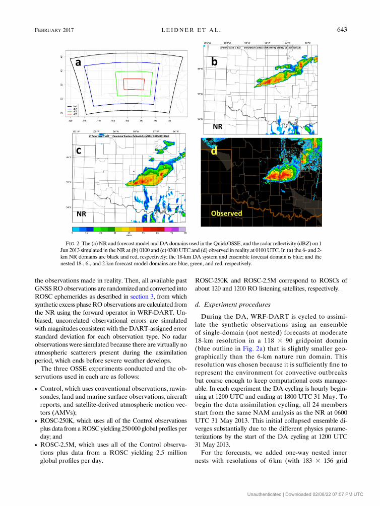
b. Nature run

The NR must be as realistic as possible since it is taken

to be the truth in the QuickOSSE framework. Since our

focus is on the development of precursors to severe con-

vection, the depiction of a realistic dryline is critical. A

6-km convection-permitting NR from 0600 UTC 31 May

to 1200 UTC 1 June 2013 was generated over the domain

outlined in black in Fig. 2a, which covers a large part of the

continental United States, with an inner 2-km nest (shown

in red inFig. 2a) that coversmost of the state ofOklahoma,

the primary area of interest for this study. Initial conditions

for the NR are provided by NAM 12-km analysis.

Convection is slower to develop and evolve by an hour

or two in the NR compared to reality, but the phe-

nomenology and evolution of the convection and asso-

ciated updraft helicity are strikingly similar to observed.

These findings are from the hourly time series of NR and

observed composite reflectivity, examples of which are

included in Fig. 2. Note the agreement of the NR

(Figs. 2b,c) to reality (Fig. 2d) is somewhat better when

shifted backward in time by 2 hours.

c. Simulation of observations

In anOSSE, simulated observationsmust be generated

with realistic coverage from the NR with added obser-

vation errors of the proper size. Conventional observa-

tions of altimeter setting, temperature, dewpoint, and

horizontal wind components are simulated by evaluating

the 6-km NR outer domain at the times and locations of

FIG. 1.GNSSRO data coverage over the NR domain for (a) all

178 rising occultations for GNSS satellite G22 during the 7.8-yr

period 20 May 2006–27 Feb 2014. (b) As in (a), but with ran-

domly rotated azimuths and with time compressed and reas-

signed to the interval 1130–1830 UTC 31May 2013. (c) As in (b),

but for the 766 occultation for all GNSS satellites during a 1-h

period (1130–1230 UTC 31 May 2013).

642 MONTHLY WEATHER REV IEW VOLUME 145

Unauthenticated | Downloaded 02/08/22 07:07 PM UTC

the observations made in reality. Then, all available past

GNSSROobservations are randomized and converted into

ROSC ephemerides as described in section 3, from which

synthetic excess phaseROobservations are calculated from

the NR using the forward operator in WRF-DART. Un-

biased, uncorrelated observational errors are simulated

withmagnitudes consistent with theDART-assigned error

standard deviation for each observation type. No radar

observations were simulated because there are virtually no

atmospheric scatterers present during the assimilation

period, which ends before severe weather develops.

The three OSSE experiments conducted and the ob-

servations used in each are as follows:

d Control, which uses conventional observations, rawin-

sondes, land and marine surface observations, aircraft

reports, and satellite-derived atmospheric motion vec-

tors (AMVs);d ROSC-250K, which uses all of the Control observations

plus data fromaROSCyielding 250000 global profiles per

day; andd ROSC-2.5M, which uses all of the Control observa-

tions plus data from a ROSC yielding 2.5 million

global profiles per day.

ROSC-250K and ROSC-2.5M correspond to ROSCs of

about 120 and 1200 RO listening satellites, respectively.

d. Experiment procedures

During the DA, WRF-DART is cycled to assimi-

late the synthetic observations using an ensemble

of single-domain (not nested) forecasts at moderate

18-km resolution in a 118 3 90 gridpoint domain

(blue outline in Fig. 2a) that is slightly smaller geo-

graphically than the 6-km nature run domain. This

resolution was chosen because it is sufficiently fine to

represent the environment for convective outbreaks

but coarse enough to keep computational costs manage-

able. In each experiment the DA cycling is hourly begin-

ning at 1200 UTC and ending at 1800 UTC 31 May. To

begin the data assimilation cycling, all 24 members

start from the same NAM analysis as the NR at 0600

UTC 31 May 2013. This initial collapsed ensemble di-

verges substantially due to the different physics parame-

terizations by the start of the DA cycling at 1200 UTC

31 May 2013.

For the forecasts, we added one-way nested inner

nests with resolutions of 6 km (with 183 3 156 grid

FIG. 2. The (a)NRand forecastmodel andDAdomains used in theQuickOSSE, and the radar reflectivity (dBZ) on 1

Jun 2013 simulated in the NR at (b) 0100 and (c) 0300UTC and (d) observed in reality at 0100UTC. In (a) the 6- and 2-

km NR domains are black and red, respectively; the 18-km DA system and ensemble forecast domain is blue; and the

nested 18-, 6-, and 2-km forecast model domains are blue, green, and red, respectively.

FEBRUARY 2017 LE IDNER ET AL . 643

Unauthenticated | Downloaded 02/08/22 07:07 PM UTC

points, green outline in Fig. 2a) and 2 km (with 318 3210 grid points, red outline in Fig. 2a). The 2-km NR

and forecast grids are identical. This allows analysis

and forecast verification without horizontal inter-

polation. To examine the impact of the observations on

forecasts of the development of the preconvective en-

vironment and subsequent convection, forecasts are

initialized after data assimilation and before convec-

tion have begun at 1400, 1600, and 1800 UTC 31 May.

These forecasts end at 1200UTC 1 June 2013, well after

the first wave of convection has ended. Since the en-

semble mean is the best estimate of the atmospheric

state, but may be dynamically unbalanced, the initial

state for each forecast is taken from the ensemble

member closest to the ensemble mean determined with

the rms normalized (actually, fractional) difference

distance metric in the space defined by the WRF state

vector. Many of these and other details of our experi-

ments mirror the standard NSSL Spring Experiment

practice.

5. Experiment results

The analyses and forecasts created for the different

experiments are validated against the corresponding

NR values.

a. Analysis impacts

Figure 3 shows snapshots from the NR, Control, and

ROSC-2.5M experiments of lower-tropospheric water

vapor—a key ingredient for severe weather. All are valid

at 1700 UTC 31 May 2013 (i.e., 4–5h before severe

weather impacted Oklahoma City), and at 1.25km above

ground level. Figure 3a shows water vapor from the NR.

The intense dryline seen in this realization of atmosphere

moisture is the yardstick against which our assimilation

experiments are compared for realism. Figure 3b and 3c

compare the effects of using conventional weather ob-

servations versus conventional weather observations plus

ROSC-2.5M observations. The ROSC-2.5M experiment

that includes the RO observations produces a water va-

por analysis (Fig. 3f) that is very much closer to the NR

snapshot (Fig. 3d) in terms of the position and strength of

the dryline than the Control experiment that uses only

conventional weather observations (Fig. 3e).

In addition to improved specification of the atmos-

pheric moisture field, assimilation of ROSC observations

improves the analysis uncertainty. Figure 4 shows the

water vapor mixing ratio analysis mean and uncertainty

at; 140mAGL valid at the start, middle, and end of the

assimilation period for the Control and ROSC-2.5M

experiments. In the ROSC-2.5M experiment the

FIG. 3. Atmospheric water vapor (g kg21, color fill) at 1.25 km (approximately 4000 ft) AGL at 1800 UTC 31 May 2013 for (a) the NR,

(b) the Control experiment analysis, and (c) the ROSC-2.5M experiment analysis. (d)–(f) Enlargement of the areas in (a)–(c) that are

marked by the black rectangles. The gray dashed circle highlights the position of the dryline in the NR and is repeated at that position in

the other panels. Note that the analyses in the DA experiments use a coarser 18-km grid than the 2-km nature run grid.

644 MONTHLY WEATHER REV IEW VOLUME 145

Unauthenticated | Downloaded 02/08/22 07:07 PM UTC

uncertainty is much less immediately after the first

assimilation cycle (cf. Figs. 4d and 4a). Then the un-

certainty continues to decrease over the course of the ex-

periment (from left to right in Fig. 4). However, in the

Control experiment, without the benefit of the additional

observations, the uncertainty increases in the strong gradi-

ent areas (cf. Figs. 4b,c and 4a). By the end of the assimi-

lation, the dryline is much stronger (i.e., there is a sharper

gradient represented by closer contours) and less uncertain

(less yellow and red) in the ROSC-2.5M experiment

(Fig. 4f) compared to the Control experiment (Fig. 4c).

The impact of ROSC observations on the analysis of

lower-tropospheric temperature is similar to the impact on

themoisture field, but the effects aremore localized. After

several hourly DA cycles, mesoscale features in the

ROSC-2.5M analyses in the vicinity of the front are more

clearly defined and represented compared to the Control

experiment (not shown). As with analysis of the moisture

field, uncertainty in the ROSC-2.5M temperature analyses

is greatly reduced compared to the Control experiment.

Assimilating the ROSC observations also improved the

fit to the conventional data. Figure 5 shows vertical profiles

of the RMS difference of dewpoint between the simulated

radiosonde observations and background (or guess) and

the analysis for the Control and ROSC-2.5M experiments.

Note that the impact on the analysis is more substantial

than on the background. The RO data consistently

improves the analysis of moisture, but during the 1-h

forecast this improvement is degraded, possibly because

there is little or no improvement in the wind analysis,

which then has a negative impact as it advects themoisture

analysis.

b. Forecast impacts

We verify the forecasts against the NR using maximum

updraft helicity (UH), convective available potential en-

ergy (CAPE), and 2m temperature.UH is computed as the

maximum value (over the hour ending at the valid time) of

H (t), where H (t) (inm2 s22) is equal to vertical velocity

times vertical vorticity integrated between two levels taken

as 850 and 500hPa in the results presented here.As in other

studies (e.g., Clark et al. 2013), UH is taken to be a di-

agnostic for subgrid-scale severe weather and indicates the

presence of rotating updrafts and, when persistent and

sufficiently intense, long-track tornadoes. Also, by exam-

ining the effects for two constellation sizes—250 000

and 2 500 000 global profiles per day—we examine

how the impact of the ROSC varies with observing

density.

Highlights of the forecast impacts are the following.

First, convective initiation and early convection mor-

phology are improved by assimilating dense RO data.

Second, most domain-averaged metrics remain signif-

icantly improved hours into the forecast. Figure 6

FIG. 4. The water vapor mixing ratio analysis uncertainty (g kg21, color fill) and analysis mean (g kg21, black contours) at; 140mAGL

valid at (a),(d) 1200; (b),(e) 1500; and (c),(f) 1800 UTC 31 May (i.e., at the end of the first, fourth, and seventh 1-h WRF-DART analysis

cycles) for (a)–(c) the Control experiment and (d)–(f) the ROSC-2.5M experiment. The ensemble standard deviation is plotted in the

colors shown by the color scale embedded on the right side of each panel, which runs from zero (blue) to 3.5 g kg21 (red), with numeric

values indicated on the right of (c) and (f).

FEBRUARY 2017 LE IDNER ET AL . 645

Unauthenticated | Downloaded 02/08/22 07:07 PM UTC

shows a number of RMS error statistics over the fore-

cast model innermost domain calculated with the WRF

Model Evaluation Toolkit (MET) Grid-Stat tool and

using the NR as verification. The evolution of the RMS

error values has a correspondence to the evolution of

the NR convection. The line of convection seen in the

NR-simulated radar reflectivity begins at 2100 UTC

31 May and becomes mature at 0100 UTC 1 June

(Fig. 2b). Errors in CAPE and 2-m temperature are

large during this period as convection develops. By

0600 UTC 1 June, the NR area of convection has sub-

stantially dissipated and largely moved out of the 2-km

verification domain toward the southeast. Another line of

convection begins to develop in the domain at 0700 UTC

1 June and reaches maturity at 1200 UTC 1 June.

Errors in CAPE and 2-m temperature are again large

during this period as convection develops. The trace

of UH RMS error corresponds approximately to the

strength of the convective activity seen in the radar

reflectivity for the first convective event in the NR.

There is no corresponding increase during the develop-

ment of the second convective event presumably because

strong UH is not present in this event. The lower

CAPE errors for the free-running ‘‘Nodata’’ forecast

(initiated at 0600 UTC) compared to the first few hours

of the 1400 UTC (and less so for the 1600 UTC) Control

and ROSC-2.5K forecasts reflect the benefit of the long

spinup time in the Nodata forecast for CAPE. This rela-

tive advantage disappears with higher data volumes

(ROSC-2.5M) and additional assimilation cycles (1600

and 1800 UTC). There are also smaller errors for the

forecast Nodata 2-m temperature past 0200 UTC 1 June,

but this is late in the forecast when the influence of the

initial conditions is reduced and may be a sampling arti-

fact that would not be present with a larger number of

forecast cases.

It should be noted the forecast results are generally

mixed and should be viewed as preliminary, in large part

due to the chaotic nature of evolving convection. First,

large samples are required to establish statistical signifi-

cance, and a single case study can only hint at forecast

impacts. Second, forecasts of convective events lack skill

both because ofmodel errors and initial errors. TheROSC

OSSEs only improve initial errors, and the forecast impact

FIG. 5. Vertical profiles of RMS differences of radiosonde dewpoint (K) to the background (O2 B, blue circles)

and to the analysis (O2 A, green diamonds) for (a) the Control experiment and (b) the ROSC-2.5M experiment.

Dashed lines give the number of observations (top axis) available (gray) and passing QC and used (black) vs

pressure level. Statistics (RMS differences and counts) are calculated over the 7DA cycles (12–18UTC 31May 2013).

646 MONTHLY WEATHER REV IEW VOLUME 145

Unauthenticated | Downloaded 02/08/22 07:07 PM UTC

quickly becomes very difficult to detect due the noise

caused by model errors.

6. Summary and conclusions

Experiments evaluating the impact of ROSCs in a

severe weather QuickOSSE suggest the potential for

high-resolution GNSS RO observations to refine the

position and intensity and to reduce the analysis

uncertainty of a dryline in the lower-tropospheric humid-

ity field, as well as of features in the lower-tropospheric

temperature field. This first mesoscale, severe weather

application/evaluation of RO data showed very positive

results for tropospheric moisture analysis and generally

positive forecast impacts, albeit in the context of a single

case study. In addition, our results suggest that ROSCs

may also improve the forecast distribution of key envi-

ronmental precursor controls for convection initiation and

intensity (e.g., CAPE; capping inversions; midlevel dry

layers; wind shear) by better analyzing the temperature

and humidity variables; and improve the forecast timing

and location of convective outbreaks.

In conclusion, our results suggest that observations

from future hypothetical large ROSCs have significant

potential to produce more accurate analyses in severe

weather environments, and therefore, better charac-

terize the environment for severe weather convective

initiation. More accurate 3D analyses of temperature

and water vapor in the lower troposphere are critical to

improved severe weather forecasts. The forecast re-

sults are encouraging but limited by sample size and the

ability of current models to forecast severe weather.

A number of caveats apply to this study. First, the

impact of RO observations on severe weather analysis

and forecasting should be examined for other diverse

cases. Second, the nominal set of observations (i.e., those

used in Control described in section 4c) does not include

radar data. The lack of radar data is justified in this study

because convection is minimal during the assimilation

period, but other cases should be chosen to study the

FIG. 6. RMS forecast error for (top) CAPE (J kg21), (middle) hourly maximum updraft helicity (UH) (m2 s22), and (bottom) 2-m

temperature (T2M, 8C) for forecasts initialized from analyses at (left) 1400, (middle) 1600, and (right) 1800 UTC 31 May 2013. In each

panel the RMS errors are shown for the Control experiment (blue), the ROSC-250K experiment (green, labeled ‘‘C250K’’), the ROSC-

2.5M experiment (red, labeled ‘‘C2.5M’’), and the free-running forecast (gray, labeled ‘‘Nodata’’, repeated from left to right panels).

Dashed lines using the same colors are plotted for the mean RMS error over the forecast period.

FEBRUARY 2017 LE IDNER ET AL . 647

Unauthenticated | Downloaded 02/08/22 07:07 PM UTC

impact of combining RO and radar data. The approach

of this study is helpful to demonstrate that the RO has

useful information, but does not demonstrate that this

information will still add value when other available

observations are thoroughly exploited. Third, the ad-

ditional, potentially valuable, impact of RO observa-

tions on correcting biases of other data types is not

included in the current study. Fourth, several aspects of

the OSSE system used here could be improved. All

aspects of an OSSE system should be tuned and vali-

dated with respect to realism (Hoffman and Atlas

2016). While the NR described in section 2a is realistic

in several aspects, only limited validation versus reality

was performed. Choices of parameterization for the

NR were made subjectively so that differences be-

tween the NR and reality were as small as possible. A

subjective comparison of simulated and observed re-

flectivity images indicated that differences among the

longer nonensemble forecasts (initialized at 1400, 1600,

and 1800 UTC) and the NR were generally larger than

differences between the NR and observed. A more thor-

ough study of the forecast differences would be desirable,

but should include additional cases. Some shortcuts to

simulating the RO observations were taken, including the

generation of tangent points, the use of the same forward

model in simulating and assimilating observations, and the

vertical thinning procedure. The WRF-DART system

used, while advanced in using the EnKF approach is

simplistic in some regards compared to an operational

system. In particular the effect of variational bias correc-

tion (mentioned above) and quality control are not pres-

ent in the experiments reported here.

Clearly there is more to do—this is a preliminary

study and the quantitative results of simulation studies

are not directly applicable to reality without thorough

calibration and validation. However, in spite of the

above caveats, the results of the current study do suggest

the potential for RO observations to improve our ability

to warn on forecast for severe weather events.

Acknowledgments. The authors thank Robert Atlas,

Richard Anthes, Jon Kirchner, and Lidia Cucurull for

helpful discussions relevant to this work. The authors

thank the journal reviewers and Thomas Jones for their

thorough and careful reviews and helpful suggestions

and comments.

APPENDIX

Acronyms and Expansions

All acronyms used in the text are defined below. Acronyms

used as units (e.g., UTC) and proper names (e.g., names of

specific institutions and systems) are not expanded in the

text.

Acronym Definition

4D-Var Four-dimensional variational data assimilation

ACM2 Asymmetrical Convective Model, version 2

AGL Above ground level

AMV Atmospheric motion vector

CAPE Convective available potential energy

COSMIC Constellation Observing System for Meteorol-

ogy, Ionosphere and Climate

DA Data assimilation

DART Data Assimilation Research Testbed

dBZ decibels of Z (reflectivity)

ECMWF European Centre for Medium-Range Weather

Forecasts

EF Enhanced Fujita scale

EnKF Ensemble Kalman filter

GNSS Global Navigation Satellite System

GPS Global positioning system

LEO Low Earth orbit

MET Model Evaluation Tools

MYJ Mellor–Yamada–Janjic

MYNN Mellor–Yamada–Nakanishi–Niino

NAM North American Mesoscale Forecast System

NCAR National Center for Atmospheric Research

NCEP National Centers for Environmental Prediction

NME NSSL Mesoscale Ensemble

NOAA National Oceanic and Atmospheric Administration

Noah NOAA/NCEP–Oregon State University–Air

Force Research Laboratory–NOAA/Office of

Hydrology land surface model

NR Nature run

NSSL National Severe Storms Laboratory (NOAA)

OSE Observing system experiment

OSSE Observing system simulation experiment

PBL Planetary boundary layer

QC Quality control

QuickOSSE Quick OSSE

RMS Root-mean-square

RO Radio occultation

ROSC RO superconstellations

RRTMG Rapid Radiative Transfer Model for GCMs

T2M 2-m temperature

TP Tangent point

UH Maximum updraft helicity

UTC Universal Time Coordinated

WRF Weather Research and Forecasting Model

YSU Yonsei University

REFERENCES

Anderson, J., T. Hoar, K. Raeder, H. Liu, N. Collins, R. Torn, and

A. Avellano, 2009: The Data Assimilation Research Testbed:

A community facility.Bull. Amer.Meteor. Soc., 90, 1283–1296,doi:10.1175/2009BAMS2618.1.

Atlas, R., and T. S. Pagano, 2014: Observing system simulation ex-

periments to assess the potential impact of proposed satellite

648 MONTHLY WEATHER REV IEW VOLUME 145

Unauthenticated | Downloaded 02/08/22 07:07 PM UTC

instruments on hurricane prediction. Imaging Spectrometry

XIX, P.Mouroulis andT. S. Pagano, Eds., International Society

for Optical Engineering (SPIE Proceedings, Vol. 9222),

doi:10.1117/12.2063648.

——, L. Bucci, B. Annane, R. Hoffman, and S. Murillo, 2015: Ob-

serving system simulation experiments to assess the potential

impact of new observing systems on hurricane forecasting.Mar.

Technol. Soc. J., 49, 140–148, doi:10.4031/MTSJ.49.6.3.

Bingham, G., and Coauthors, 2013: Rapidly updated hyperspectral

sounding and imaging data for severe storm prediction. Infrared

Remote Sensing and Instrumentation XXI, M. Strojnik Scholl and

Gonzalo Páez, Eds., International Society for Optical Engineer-

ing (SPIE Proceedings, Vol. 8867), doi:10.1117/12.2030687.

Bluestein, H. B., J. C. Snyder, and J. B. Houser, 2015: Amultiscale

overview of the El Reno, Oklahoma, tornadic supercell of

31 May 2013. Wea. Forecasting, 30, 525–552, doi:10.1175/

WAF-D-14-00152.1.

Chen, S. Y., C. Y. Huang, Y. H. Kuo, Y. R. Guo, and

S. Sokolovskiy, 2009: Assimilation of GPS refractivity from

FORMOSAT-3/COSMIC using a nonlocal operator with

WRF 3DVAR and its impact on the prediction of a typhoon

event. Terr. Atmos. Oceanic Sci., 20, 133–154, doi:10.3319/

TAO.2007.11.29.01(F3C).

Chen, Y.-C., M.-E. Hsieh, L.-F. Hsiao, Y.-H. Kuo, M.-J. Yang,

C.-Y. Huang, and C.-S. Lee, 2015: Systematic evaluation of

the impacts of GPSRO data on the prediction of typhoons

over the northwestern Pacific in 2008–2010. Atmos. Meas.

Tech., 8, 2531–2542, doi:10.5194/amt-8-2531-2015.

Chou, M.-D., and M. J. Suarez, 1999: A solar radiation parameter-

ization (CLIRAD-SW) for atmospheric studies (Tech. Memo.

1999-104606). A Solar Radiation Parameterization for Atmo-

spheric Studies, M.-D. Chou and M. J. Suarez, Eds., Technical

Report Series onGlobal Modeling andData Assimilation, Vol.

15, NASA, Goddard Space Flight Center, Greenbelt, MD, 38

pp. [Available online at http://www2.mmm.ucar.edu/wrf/users/

phys_refs/SW_LW/Goddard_part1.pdf.]

——,——, X.-Z. Liang, andM.M.-H. Yan, 2001: A thermal infrared

radiation parameterization for atmospheric studies (Tech.

Memo. 2001-104606). A Thermal Infrared Radiation Parame-

terization for Atmospheric Studies, M. J. Suarez, Ed., Technical

Report Series on Global Modeling and Data Assimilation, Vol.

19,NASA,Goddard Space FlightCenter,Greenbelt,MD, 55 pp.

[Available online at http://www2.mmm.ucar.edu/wrf/users/

phys_refs/SW_LW/Goddard_part2.pdf.]

Clark, A. J., J. Gao, P. T. Marsh, T. Smith, J. S. Kain, J. Correia, Jr.,

M. Xue, and F. Kong, 2013: Tornado pathlength forecasts

from 2010 to 2011 using ensemble updraft helicity. Wea.

Forecasting, 28, 387–407, doi:10.1175/WAF-D-12-00038.1.

COESA, 1976: U.S. Standard Atmosphere, 1976. NOAA, 227 pp.

Cucurull, L., and J. C. Derber, 2008: Operational implementation

of COSMIC observations into NCEP’s global data assimila-

tion system. Wea. Forecasting, 23, 702–711, doi:10.1175/

2008WAF2007070.1.

——, ——, R. Treadon, and R. J. Purser, 2007: Assimilation of

Global Positioning System radio occultation observations into

NCEP’s global data assimilation system.Mon. Wea. Rev., 135,

3174–3193, doi:10.1175/MWR3461.1.

Data Assimilation Research Testbed, 2016: DART Lanai Release

Notes. NCAR, Boulder, CO, accessed 7 April 2014. [Available

online at http://www.image.ucar.edu/DAReS/DART/Lanai_

release.html. ]

Ek, M. B., K. E. Mitchell, Y. Lin, E. Rogers, P. Grunmann, V. Koren,

G. Gayno, and J. D. Tarpley, 2003: Implementation of Noah land-

surface model advances in the NCEP operational mesoscale Eta

model. J. Geophys. Res., 108, 8851, doi:10.1029/2002JD003296.

Fujita, T., D. J. Stensrud, and D. C. Dowell, 2007: Surface data

assimilation using an ensemble Kalman filter approach with

initial condition and model physics uncertainties. Mon. Wea.

Rev., 135, 1846–1868, doi:10.1175/MWR3391.1.

Gilliam, R. C., and J. E. Pleim, 2010: Performance assessment of

new land surface and planetary boundary layer physics in the

WRF-ARW. J. Appl. Meteor. Climatol., 49, 760–774,

doi:10.1175/2009JAMC2126.1.

Grell, G. A., and S. R. Freitas, 2014: A scale and aerosol aware

stochastic convective parameterization for weather and air

quality modeling. Atmos. Chem. Phys., 14, 5233–5250,

doi:10.5194/acp-14-5233-2014.

Greybush, S. J., E. Kalnay, T. Miyoshi, K. Ide, and B. R. Hunt,

2011: Balance and ensemble Kalman filter localization

techniques. Mon. Wea. Rev., 139, 511–522, doi:10.1175/

2010MWR3328.1.

Hajj, G. A., E. R. Kursinski, L. J. Romans, W. I. Bertiger, and S. S.

Leroy, 2002: A technical description of atmospheric sounding

by GPS occultation. J. Atmos. Sol.-Terr. Phys., 64, 451–469,

doi:10.1016/S1364-6826(01)00114-6.

Healy, S. B., 2008: Forecast impact experiment with a constellation

of GPS radio occultation receivers. Atmos. Sci. Lett., 9, 111–

118, doi:10.1002/asl.169.

Hoffman, R. N., and R. Atlas, 2016: Future observing system

simulation experiments. Bull. Amer. Meteor. Soc., 97, 1601–

1616, doi:10.1175/BAMS-D-15-00200.1.

Hong, S.-Y., Y. Noh, and J. Dudhia, 2006: A new vertical diffusion

package with an explicit treatment of entrainment processes.

Mon. Wea. Rev., 134, 2318–2341, doi:10.1175/MWR3199.1.

Iacono, M. J., J. S. Delamere, E. J. Mlawer, M. W. Shephard, S. A.

Clough, and W. D. Collins, 2008: Radiative forcing by long-

lived greenhouse gases: Calculations with the AER radiative

transfer models. J. Geophys. Res., 113, D13103, doi:10.1029/

2008JD009944.

Janjic, Z., 1994: The step-mountain Eta coordinate model: Further

developments of the convection, viscous sublayer, and turbulence

closure schemes. Mon. Wea. Rev., 122, 927–945, doi:10.1175/

1520-0493(1994)122,0927:TSMECM.2.0.CO;2.

——, 2002: Nonsingular implementation of the Mellor-Yamada

level 2.5 scheme in the NCEP Meso model. Office Note 437,

NCEP, Washington, DC, 61 pp.

Jirak, I. L., and Coauthors, 2014: An overview of the 2013 NOAA

Hazardous Weather Testbed Spring Forecasting Experiment.

26th Conf. onWeather Analysis and Forecasting/22nd Conf. on

Numerical Weather Prediction, Atlanta, GA, Amer. Meteor.

Soc., J11.1. [Available online at https://ams.confex.com/ams/

94Annual/webprogram/Paper239754.html.]

Jones, T. A., J. A. Otkin, D. J. Stensrud, and K. Knopfmeier, 2013:

Assimilation of satellite infrared radiances and Doppler radar

observations during a cool season observing system simulation

experiment. Mon. Wea. Rev., 141, 3273–3299, doi:10.1175/

MWR-D-12-00267.1.

——, D. Stensrud, L. Wicker, P. Minnis, and R. Palikonda, 2015:

Simultaneous radar and satellite data storm-scale assimilation

using an ensemble Kalman filter approach for 24 May 2011.

Mon.Wea. Rev., 143, 165–194, doi:10.1175/MWR-D-14-00180.1.

——, K. Knopfmeier, D. Wheatley, G. Creager, P. Minnis, and

R. Palikonda, 2016: Storm-scale data assimilation and ensemble

forecasting with the NSSL experimental warn-on-forecast sys-

tem. Part II: Combined radar and satellite data experiments.

Wea. Forecasting, 31, 297–327, doi:10.1175/WAF-D-15-0107.1.

FEBRUARY 2017 LE IDNER ET AL . 649

Unauthenticated | Downloaded 02/08/22 07:07 PM UTC

Kain, J. S., 2004: The Kain–Fritsch convective parameterization:

An update. J. Appl. Meteor., 43, 170–181, doi:10.1175/

1520-0450(2004)043,0170:TKCPAU.2.0.CO;2.

——, and J. M. Fritsch, 1993: Convective parameterization for

mesoscale models: The Kain–Fritsch scheme. The Represen-

tation of Cumulus Convection in Numerical Models, Meteor.

Monogr., No. 24, Amer. Meteor. Soc., 165–170.

Kalnay, E., 2002: Atmospheric Modeling, Data Assimilation, and

Predictability. Cambridge University Press, 364 pp.

Kerr, C. A., D. J. Stensrud, and X. Wang, 2015: Assimilation of

cloud-top temperature and radar observations of an idealized

splitting supercell using an observing system simulation ex-

periment. Mon. Wea. Rev., 143, 1018–1034, doi:10.1175/

MWR-D-14-00146.1.

Kunii, M., H. Seko, M. Ueno, Y. Shoji, and T. Tsuda, 2012: Impact

of assimilation of GPS radio occultation refractivity on the

forecast of Typhoon Usagi in 2007. J. Meteor. Soc. Japan, 90,

255–273, doi:10.2151/jmsj.2012-207.

Kursinski, E. R., andG. A. Hajj, 2001: A comparison of water vapor

derived from GPS occultations and global weather analyses.

J. Geophys. Res., 106, 1113–1138, doi:10.1029/2000JD900421.

——, ——, J. T. Schofield, R. P. Linfield, and K. R. Hardy, 1997:

Observing Earth’s atmosphere with radio occultation mea-

surements using the Global Positioning System. J. Geophys.

Res., 102, 23 429–23 465, doi:10.1029/97JD01569.

Lambrigtsen, B. H., 2015: Progress in developing a geostationary

microwave sounder. 11th Annual Symp. on New Generation

Operational Environmental Satellite Systems, Phoenix, AZ,

Amer. Meteor. Soc., J19.3. [Available online at https://ams.

confex.com/ams/95Annual/webprogram/Paper267078.html.]

Li, X., F. Zus, C. Lu, T. Ning, G. Dick, M. Ge, J. Wickert, and

H. Schuh, 2015: Retrieving high-resolution tropospheric gra-

dients from multiconstellation GNSS observations. Geophys.

Res. Lett., 42, 4173–4181, doi:10.1002/2015GL063856.

Liu, H., J. Anderson, Y.-H. Kuo, C. Snyder, and A. Caya, 2008:

Evaluation of a nonlocal quasi-phase observation operator in

assimilation of CHAMP radio occultation refractivity withWRF.

Mon. Wea. Rev., 136, 242–256, doi:10.1175/2007MWR2042.1.

Ma, Z., Y.-H. Kuo, F. M. Ralph, P. J. Neiman, G. A. Wick,

E. Sukovich, and B. Wang, 2011: Assimilation of GPS radio

occultation data for an intense atmospheric river with the

NCEP regional GSI system. Mon. Wea. Rev., 139, 2170–2183,

doi:10.1175/2011MWR3342.1.

Maschhoff, K., 2015: MISTiC winds, a distributed architecture

approach to dynamic weather observations. Fifth Conf. on

Transition of Research to Operations, Phoenix, AZ, Amer.

Meteor. Soc., 2.2. [Available online at https://ams.confex.com/

ams/95Annual/webprogram/Paper269044.html.]

Melbourne, W. G., and Coauthors, 1994: The application of space-

borne GPS to atmospheric limb sounding and global change

monitoring. JPLPubl. 94-18,NASAJet PropulsionLaboratory,

Pasadena, CA, 147 pp. [Available online at https://ntrs.nasa.

gov/archive/nasa/casi.ntrs.nasa.gov/19960008694.pdf.]

Nakanishi, M., and H. Niino, 2006: An improved Mellor–Yamada

Level-3 model: Its numerical stability and application to a

regional prediction of advection fog. Bound.-Layer Meteor.,

119, 397–407, doi:10.1007/s10546-005-9030-8.

——, and ——, 2009: Development of an improved turbulence

closure model for the atmospheric boundary layer. J. Meteor.

Soc. Japan, 87, 895–912, doi:10.2151/jmsj.87.895.

Pan, Y., K. Zhu, M. Xue, X. Wang, M. Hu, S. G. Benjamin, S. S.

Weygandt, and J. S. Whitaker, 2014: A GSI-based coupled

EnSRF-En3DVar hybrid data assimilation system for the oper-

ational rapid refresh model: Tests at a reduced resolution.Mon.

Wea. Rev., 142, 3756–3780, doi:10.1175/MWR-D-13-00242.1.

Pleim, J. E., 2007a: A combined local and nonlocal closure

model for the atmospheric boundary layer. Part I: Model

description and testing. J. Appl. Meteor. Climatol., 46,

1383–1395, doi:10.1175/JAM2539.1.

——, 2007b: A combined local and nonlocal closure model for the

atmospheric boundary layer. Part II: Application and evalu-

ation in a mesoscale meteorological model. J. Appl. Meteor.

Climatol., 46, 1396–1409, doi:10.1175/JAM2534.1.

——, and A. Xiu, 2003: Development of a land surface model. Part

II: Data assimilation. J. Appl. Meteor., 42, 1811–1822,

doi:10.1175/1520-0450(2003)042,1811:DOALSM.2.0.CO;2.

Poli, P., 2004: Effects of horizontal gradients on GPS radio occul-

tation observation operators. II: A fast atmospheric re-

fractivity gradient operator (FARGO).Quart. J. Roy. Meteor.

Soc., 130, 2807–2825, doi:10.1256/qj.03.229.Schwartz, C. S., G. S. Romine, R. A. Sobash, K. R. Fossell, and

M. L. Weisman, 2015a: NCAR’s experimental real-time con-

vection-allowing ensemble prediction system. Wea. Fore-

casting, 30, 1645–1654, doi:10.1175/WAF-D-15-0103.1.

——, ——, M. L. Weisman, R. A. Sobash, K. R. Fossell, K. W.

Manning, and S. B. Trier, 2015b: A real-time convection-

allowing ensemble prediction system initialized by mesoscale

ensemble Kalman filter analyses. Wea. Forecasting, 30, 1158–

1181, doi:10.1175/WAF-D-15-0013.1.

Skamarock, W. C., and J. B. Klemp, 2008: A time-split non-

hydrostatic atmospheric model for weather research and

forecasting applications. J. Comput. Phys., 227, 3465–3485,

doi:10.1016/j.jcp.2007.01.037.

——, and Coauthors, 2008: A description of the Advanced

Research WRF version 3. NCAR Tech. Note NCAR/

TN-4751STR, 113 pp., doi:10.5065/D68S4MVH.

Snook, N., M. Xue, and Y. Jung, 2015: Multiscale EnKF assimila-

tion of radar and conventional observations and ensemble

forecasting for a tornadic mesoscale convective system. Mon.

Wea. Rev., 143, 1035–1057, doi:10.1175/MWR-D-13-00262.1.

Sokolovskiy, S., Y.-H. Kuo, and W. Wang, 2005: Assessing the

accuracy of a linearized observation operator for assimilation

of radio occultation data: Case simulations with a high-

resolution weather model. Mon. Wea. Rev., 133, 2200–2212,

doi:10.1175/MWR2948.1.

Stensrud, D. J., J.-W. Bao, and T. T. Warner, 2000: Using initial

condition and model physics perturbations in short-range en-

semble simulations of mesoscale convective systems. Mon. Wea.

Rev., 128, 2077–2107, doi:10.1175/1520-0493(2000)128,2077:

UICAMP.2.0.CO;2

——, and Coauthors, 2009: Convective-scale warn-on-forecast

system: A vision for 2020. Bull. Amer. Meteor. Soc., 90,

1487–1499, doi:10.1175/2009BAMS2795.1.

Tewari, M., and Coauthors, 2004: Implementation and verification of

the unified Noah land surface model in the WRF model. 20th

Conf. on Weather Analysis and Forecasting/16th Conf. on Nu-

merical Weather Prediction, Seattle, WA, Amer. Meteor. Soc.,

14.2a. [Available online at https://ams.confex.com/ams/84Annual/

techprogram/paper_69061.htm.]

Thompson, G., R. M. Rasmussen, and K. Manning, 2004: Explicit

forecasts of winter precipitation using an improved bulk

microphysics scheme. Part I: Description and sensitivity

analysis. Mon. Wea. Rev., 132, 519–542, doi:10.1175/

1520-0493(2004)132,0519:EFOWPU.2.0.CO;2.

——, P. R. Field, R. M. Rasmussen, and W. D. Hall, 2008: Explicit

forecasts of winter precipitation using an improved bulk

650 MONTHLY WEATHER REV IEW VOLUME 145

Unauthenticated | Downloaded 02/08/22 07:07 PM UTC

microphysics scheme. Part II: Implementation of a new

snow parameterization. Mon. Wea. Rev., 136, 5095–5115,

doi:10.1175/2008MWR2387.1.

Tiedtke, M., 1989: A comprehensive mass flux scheme for cumulus pa-

rameterization in large-scale models. Mon. Wea. Rev., 117, 1779–

1800, doi:10.1175/1520-0493(1989)117,1779:ACMFSF.2.0.CO;2.

Ware, R., and Coauthors, 1996: GPS sounding of the atmosphere

from low earth orbit: Preliminary results. Bull. Amer. Meteor.

Soc., 77, 19–40, doi:10.1175/1520-0477(1996)077,0019:

GSOTAF.2.0.CO;2.

Weisman, M. L., and Coauthors, 2015: The Mesoscale Pre-

dictability Experiment (MPEX). Bull. Amer. Meteor. Soc., 96,2127–2149, doi:10.1175/BAMS-D-13-00281.1.

Wheatley, D. M., K. H. Knopfmeier, T. A. Jones, and G. J.

Creager, 2015: Storm-scale data assimilation and ensemble

forecasting with the NSSL experimental warn-on-forecast

system. Part I: Radar data experiments.Wea. Forecasting, 30,

1795–1817, doi:10.1175/WAF-D-15-0043.1.

Wurman, J., K. Kosiba, P. Robinson, and T. Marshall, 2014: The

role of multiple-vortex tornado structure in causing storm

researcher fatalities. Bull. Amer. Meteor. Soc., 95, 31–45,

doi:10.1175/BAMS-D-13-00221.1.

Xiu, A., and J. E. Pleim, 2001: Development of a land surface

model. Part I: Application in a mesoscale meteorological

model. J. Appl. Meteor., 40, 192–209, doi:10.1175/

1520-0450(2001)040,0192:DOALSM.2.0.CO;2.

Yussouf, N., J. Gao, D. J. Stensrud, and G. Ge, 2013a: The impact of

mesoscale environmental uncertainty on the prediction of a

tornadic supercell storm using ensemble data assimilation ap-

proach. Adv. Meteor., 2013, 731647, doi:10.1155/2013/731647.——, E. R. Mansell, L. J. Wicker, D. M. Wheatley, and D. J.

Stensrud, 2013b: The ensemble Kalman filter analyses and

forecasts of the 8 May 2003 Oklahoma City tornadic su-

percell storm using single- and double-moment micro-

physics schemes. Mon. Wea. Rev., 141, 3388–3412,

doi:10.1175/MWR-D-12-00237.1.

Zhang, C., Y. Wang, and K. Hamilton, 2011: Improved representation

of boundary layer clouds over the southeast Pacific inARW-WRF

using amodifiedTiedtke cumulus parameterization scheme.Mon.

Wea. Rev., 139, 3489–3513, doi:10.1175/MWR-D-10-05091.1.

Zou, X., Y.-H. Kuo, and Y.-R. Guo, 1995: Assimilation of atmo-

spheric radio refractivity using a nonhydrostatic adjoint

model. Mon. Wea. Rev., 123, 2229–2250, doi:10.1175/

1520-0493(1995)123,2229:AOARRU.2.0.CO;2.

FEBRUARY 2017 LE IDNER ET AL . 651

Unauthenticated | Downloaded 02/08/22 07:07 PM UTC