a self-adaptive ant colony system for semantic query...
TRANSCRIPT
Computación y Sistemas Vol. 13 No. 4, 2010, pp 433-448 ISSN 1405-5546
A Self-Adaptive Ant Colony System for Semantic Query Routing Problem in P2P Networks
Sistema de Colonia de Hormigas Autoadaptativo para el Problema de Direccionamiento de Consultas Semánticas en Redes P2P
Claudia Gómez Santillán1,2, Laura Cruz Reyes2, Eustorgio Meza Conde1, Elisa Schaeffer3
and Guadalupe Castilla Valdez2 1Centro de Investigación en Ciencia Aplicada y Tecnología Avanzada del Instituto Politécnico Nacional (CICATA- IPN).
Carretera Tampico-Puerto Industrial Altamira, Km.14.5. Altamira,Tamps.,México. 2Instituto Tecnológico de Ciudad Madero (ITCM). 1ro. de Mayo y Sor Juana I. de la Cruz s/n CP. 89440, Tamaulipas, México.
3 Facultad de Ingeniería Mecánica y Eléctrica (FIME-UANL), Avenida Universidad s/n. Cd. Universitaria, CP. 66450, San Nicolás de los Garza, N.L. México.
[email protected], [email protected], [email protected], [email protected], [email protected].
Article received on July 17, 2009; accepted on November 05, 2009
Abstract In this paper, we present a new algorithm to route text queries within a P2P network, called Neighboring-Ant Search (NAS) algorithm. The algorithm is based on the Ant Colony System metaheuristic and the SemAnt algorithm. More so, NAS is hybridized with local environment strategies of learning, characterization, and exploration. Two Learning Rules (LR) are used to learn from past performance, these rules are modified by three new Learning Functions (LF). A Degree-Dispersion-Coefficient (DDC) as a local topological metric is used for the structural characterization. A variant of the well-known one-step Lookahead exploration is used to search the nearby environment. These local strategies make NAS self-adaptive and improve the performance of the distributed search. Our results show the contribution of each proposed strategy to the performance of the NAS algorithm. The results reveal that NAS algorithm outperforms methods proposed in the literature, such as Random-Walk and SemAnt. Keywords: Search Process, Internet, Complex Network, Ant Colony System, Local Environment, Neighbor. Resumen En este documento, proponemos un nuevo algoritmo para ruteo de consultas textuales dentro de una red P2P, llamado Neighboring-Ant Search (NAS). El algoritmo está basado en la metaheurística Ant Colony System (ACS) y el algoritmo SemAnt. Además, NAS está hibridizado con estrategias del ambiente local de aprendizaje, caracterización y exploración. Dos reglas de aprendizaje (LR) son usadas para aprender del rendimiento pasado, esas reglas son modificadas por tres Funciones de Aprendizaje (LF). Un Coeficiente de Dispersión del Grado (DDC) es usado como una métrica topológica local para la caracterización estructural. Una adaptación del bien conocido método de exploración de adelanto (one-step Lookahead) es usado para explorar el ambiente cercano. Estas estrategias locales proveen a NAS una capacidad auto-adaptativa que mejora el rendimiento de la búsqueda distribuida. Los resultados experimentales muestran la contribución de cada estrategia propuesta para el rendimiento del algoritmo NAS. Estos resultados revelan que el algoritmo NAS obtiene mejores resultados que los algoritmos propuestos en la literatura existente tales como Random-Walk y SemAnt. Palabras Clave: Proceso de Búsqueda, Internet, Redes Complejas, Sistema de Colonia de Hormigas, Ambiente Local, Vecindad.
1 Introduction The popularity of peer-to-peer (P2P) systems is motivated by the benefits offered to the end user. In contrast to the traditional Web, a P2P system does not need to rely on any dedicated centralized servers, which makes P2P networks reliable and fault tolerant. Hence a user can easily join a network and leave when necessary, giving rise to
434 Claudia Gómez Santillán, et al.
Computación y Sistemas Vol. 13 No. 4, 2010, pp 433-448 ISSN 1405-5546
unstructured self-organizing networks. Due to the unstructured nature, these applications often employ a flooding-based data search mechanism, which generates severe communication overhead and limits the growth of P2P systems. These systems together with the underlying Internet are considered complex dynamic distributed networks for their size and constantly evolving interconnectivity. In complex dynamic distributed networks, global knowledge collection is not a feasible approach to handle queries on shared resources. In these circumstances, each query needs to determine locally its behavior, without resorting to a global control mechanism.
Digital technologies and new standards make it possible to produce music, movies, pictures, images, and textual information in a digital form with reasonable quality. Internet is the essential, cheapest and most convenient way to manage digital files, to sell, buy, and share digital content. Such a popular application like the World Wide Web (WWW) has not been convenient enough to share files. Sharing content on the WWW requires infrastructure (a HTTP server) and makes it difficult for individual users to share their files in an easy and independent way. The files published on the WWW are available for search only after their respective sites are crawled and indexed by existing centralized search engines. Since such operations may take a significant amount of time, users have no direct control over the published files to make them available for immediate search. These disadvantages make the use of traditional applications for file sharing complicated [13].
In 1999 the P2P systems arose as a response to the increased demand for file sharing. These systems are formed by interconnected peers that offer their resources to other peers within the network. The participants connect and disconnect constantly, producing changes in the structure of the network. Due to the unstructured nature, applications mainly employ flooding-based data search mechanisms. Flooding-based search generates vast amounts of Internet traffic that limits the growth of peer-to-peer systems. The obvious problems that appeared with the growing popularity of peer-to-peer file sharing systems are two: a) the poor accuracy of the information search and b) the traffic caused by the flooding-based search. Measurements have shown that peer-to-peer systems are the main source of Internet traffic [13],[10],[11], making the development of new approaches to avoid flooding an important research challenge.
The Semantic Query Routing Problem consists in each peer deciding, based on a keyword in the query, to which neighboring peer to resend the text query. To avoid flooding, the goal is to maximize the number and the quality of query results, while minimizing the use of the resources of the network. Existing approaches for query routing in P2P networks range from simple broadcasting techniques to sophisticated methods [13],[10],[11]. Due to the fact that P2P networks are based on non-central authorities and high-growing dimension, the challenge for query routing is the development of methods that adapt themselves to dynamic environments. Such intelligent adaptation must be based only on the local knowledge of each peer. Among the intelligent mechanisms successfully applied to several problems in distributed systems, lie the ant-colony methods. The metaheuristic of Ant Colony System, proposed by Dorigo [12], solves optimization problems based on graphs. Many ant algorithms have been specifically designed for handling routing tables in telecommunications. However, there are very few ant algorithms for handling routing tables in the Semantic Query Routing Problem [10].
In this paper, we present a novel algorithm for distributed text query routing. The algorithm, called the Neighboring-Ant Search (NAS), is based on two well-known ant algorithms: the Ant Colony System [7] and the SemAnt [10]. Additionally, NAS is hybridized with local strategies of learning, characterization, and exploration. Three functions are employed to learn from past performance. The first function is used to evaluate the NAS performance based on the found and expected results. The second function qualifies the NAS performance based on the available time for the searching. The third function qualifies each peer depending on the distance towards a previously found resource. A topological metric based on the number of connections of each peer is used for the structural characterization. An adaptation of the well-known one-step Lookahead search is used to explore the neighbor peers of the nearby environment [11]. These three strategies contribute with the main goal of the application which is to find a greater amount of resources in the least amount of time.

A Self-Adaptive Ant Colony System for Semantic Query Routing Problem in P2P Networks 435
Computación y Sistemas Vol. 13 No. 4, 2010, pp 433-448 ISSN 1405-5546
2 Background In order to place the research in context, this section is divided in four parts. The first part defines, explains, and models the peer-to-peer complex networks. The second part explains and formally defines the Semantic Query Routing Problem. The third part explains and defines the Lookahead exploration and the Degree-Dispersion-Coefficient local metric. The last part refers to the Random-Walk algorithm. 2.1 Peer-to-Peer Complex Networks P2P systems are formed by interconnected peers that offer their resources to other peers within the network. Hence a P2P network is a distributed system that can be modeled as a graph. Each peer in the network is represented by a node (also called a vertex) of the graph. The interactions among the peers are represented by the connections (also called the edges) of the graph. In P2P networks, the nodes are capable of self-organization for the purpose of sharing resources, without requiring the mediation or support of a server or centralized authority [2].
More so a P2P system, together with the underlying communication network (typically Internet), forms a complex system that requires autonomous operation through mechanisms of intelligent search [10]. Amaral [1] published a classification for different types of systems and categorized them into simple, complicated, and complex systems. Complex systems are those systems that have (typically) a very large number of components, the connections among them may evolve over time, and the roles of the components may vary. In many studies, complex systems are modeled as networks, giving rise to the concept of complex networks and, within this context, the term P2P Complex Networks.
One of the main motivations for modeling systems as P2P complex networks is the flexibility and generality of the abstract representation that allows handling properties such as dynamic topology in a natural way. A recent methodology for modeling complex systems, called Autonomous Oriented Computing (AOC), was proposed by Liu [12]. AOC consists in the formulation of a tuple that represents the general model of the system, i.e.: <e1, e2,…,ei,…,eN, E,Φ>, where e1,e2,…,ei,…,eN is a subset of size N of autonomous entities, E is the environment in which the entities reside, and Φ is the objective function of the global system. Each entity is a basic element with a well-defined goal within the complex system. To achieve its goal, it has attributes that describe its behavior rules, current state, and an evaluation function. We use the AOC notation to model P2P systems as follows: i) the entities are the agents that surf in the network with the objective of finding resources; ii) the environment is the P2P network and iii) the objective function is to find the maximal set of resources in the shortest possible time. A more detailed description of our querying system based on intelligent agents is given in Section 4. 2.2 The Semantic Query Routing Problem The problem of locating textual information in a P2P network over the Internet is known as Semantic Query Routing Problem (SQRP). The goal of SQRP is to determine the shortest paths from a node that issues a query to nodes that can appropriately answer it (by providing the requested information). The query traverses the network moving from the initiating node to a neighboring node and then to a neighbor of the neighbor and so forth until it locates the requested resource (or gives up in its absence). This type of propagation is known as flooding and it is the most common search strategy in P2P networks. Algorithms for SQRP must consider several factors, ranging from hardware and software characteristics to user behavior. Due to its complexity [10],[1],[12],[6], solutions proposed to SQRP typically limit to special cases. Yang et al. [6] propose AntSearch that controls the quantity of flooding using a simple learning technique, whereas Michlmayr [10] proposes the SemAnt algorithm for learning from user behavior.
Formally, SQRP is defined with the description of an Instance and an Objective that must be satisfied by a solution algorithm such as the ant-based algorithm proposed in this work. Instance: given a P2P network represented by a graph T, a set of contents distributed in the nodes called repositories R, and a set of semantic queries Q launched by the nodes. Each query can be launched from any node in the time T
0, ∀T
0 ∈ Z, assuming a discrete-time
process. The node that originally launches a query (or receives a query from other node) in time T0+i, ∀i ∈ Z+
∪0, can locally process the query and/or forward a copy of the query to a set of nearby nodes at time T0+(i+1).
The query processing finishes when a stop condition has been satisfied, whether either the maximal quantity of
436 Claudia Gómez Santillán, et al.
Computación y Sistemas Vol. 13 No. 4, 2010, pp 433-448 ISSN 1405-5546
resources has been found or th time-to-live value specified for the query is reached. Objective: find a set of paths among the nodes launching the queries and the nodes containing the resources, such that the quantity of found resources is maximized and the quantity of steps given to find the resources is minimized.
2.3 Lookahead and the Degree-Dispersion-Coefficient A node i is a neighbor of a node j if the two nodes i and j are connected by an edge (i, j) in the graph that models the system. The set of all neighbors of a node i is denoted by ( )iΓ . In an undirected simple graph, that is, a graph in which the edges are considered bidirectional communication channels and each pair of nodes may be connected by at most one edge, the degree of a node is the number of neighbors it has.
A well-known strategy based on local information is the one-step Lookahead exploration method [11]. Lookahead is employed in algorithms to examine neighboring resources up to a certain level before deciding how to proceed with the search. In this work, we assume that each node knows the resources of the first-level neighbors.
In order to locally focus the exploration strategy we use the Degree-Dispersion-Coefficient (DDC) function [14]. DDC is based on local information that through the dispersion of the degree of a node measures the differences between the degree of a node and the degrees of its neighbors, this is:
( )( )( )iDDC ii
σµ
= , ( 1 )
Where the degree variation of the set ( )i i∪ Γ [ ]2 2
( )( )j i i i
j i
i
k ki
N
µ µσ ∈Γ
− + −=
∑, the average degree found in the
set i ∪ Γ(i) ( )( )j i
j i
i
k ki
Nµ ∈Γ
+=
∑ , Ni is the number of nodes in i ∪ Γ(i), and, ki and kj are the degree of nodes i and j
respectively. 2.4 Random-Walk Algorithm The Random-Walk (RW) search algorithm is a blind search technique where the nodes of the network possess no information on the location or contents of the requested resource, unless the resource resides in the node itself . Let G be a graph that models the network and v a node in G. A T-hop Random-Walk from v in G is a sequence of dependent random variables X0,..., XT defined as follows: X0 = v with probability 1 and for each i = 1,...,T, the value for Xi is selected uniformly at random among the nodes in 1( )iX −Γ , that is, among the neighbors of the node of the preceding step. In others words, a Random-Walk begins at a node and on each step moves to a neighbor of the current node, until it arrives to a node that meets the goal. In our P2P model, the goal is met when a node contains the requested resource [3]. Optionally, one could include the DCC function into the Random-Walk algorithm. A simple modification to include such a structural preferentiality is to choose uniformly at random two neighbors, calculate their DCC values, and move on to the neighbor with higher DCC. 3 Related Work
The success of SQR algorithms in P2P file-sharing networks lies on search mechanisms that have received special attention [10][6]. We summarize here some of the most relevant proposals for semantic query routing using Ant-Colony Algorithms. These algorithms are based mainly on a learning structure named pheromone. This structure is used for establishing indirect communication between ants about their past performance. The pheromone table (τ) is used as a query routing table.
Michlmayr [10] proposes a distributed SQRP algorithm for P2P networks called SemAnt and includes an evaluation of the parameter configuration that affects the performance of the algorithm. Michlmayr aims for an

A Self-Adaptive Ant Colony System for Semantic Query Routing Problem in P2P Networks 437
Computación y Sistemas Vol. 13 No. 4, 2010, pp 433-448 ISSN 1405-5546
optimal ratio between network traffic and quantity of results and compares the performance of SemAnt with the Random-Walk algorithm using the following metrics: i) Resource Usage define as the number of links traveled for each query within a given period of time, ii) Hit Rate defines as the number of resource found for each query within a given period of time, and iii) Efficiency defined as the ratio of resource usage to hit rate. Dividing the number of links traveled by the number of resources found, gives the average number of links traveled to find one resource.
Yang et al. [6] propose an algorithm called AntSearch for non-structured P2P networks. In AntSearch, each pair of nodes stores information on the level of success of past queries as well as on the pheromone levels of the immediate neighbors. The work of Yang et al. was motivated by the need to improve search performance in terms of the traffic in the network and the level of information recovery. Yang et al. use three metrics to measure the performance of the AntSearch. One is the number of searched files for a query with a required number of results, given N as: a good search algorithm should retrieve the number of results over but close to N. The second one is the per result costs that defines the total amount of query messages divided by the number of searched results; this metric measures how many average query messages are generated to gain a result. Finally, search latency is defined as the total time taken by the algorithm.
Di Caro and Dorigo [4] propose AntNet that is designed for packet-switched networks. The ants collaborate in building routing tables that adapt to current traffic in the network, with the aim of optimizing the performance of the entire network. AntNet uses global information on the nodes of the network in order to choose the destination nodes. Di Caro and Dorigo focused on standard metrics for performance evaluation, considering only sessions with equal costs, benefits and priority and without the possibility of requests for special services like real-time. In AntNet framework, the main measures are: i) throughput correctly delivered bits/sec, ii) delay distribution for data packets (sec), and iii) network capacity usage for data and routing packets, expressed as the sum of the used link capacities divided by the total available link capacity.
Most relevant aspects of former works have been incorporated into the proposed NAS algorithm. The framework of AntNet algorithm is modified to correspond to the problem conditions: in AntNet the final addresses are known, while NAS algorithm does not know a priori the nodes where the resources are located. On the other hand and different to AntSearch, the SemAnt algorithm and NAS are focused on the same problem conditions, and both use algorithms based on AntNet algorithm. However, the difference between the SemAnt and NAS is that SemAnt only learns from past experience, whereas NAS takes advantage of the local environment. This means that the search in NAS takes place in terms of the classic local exploration method of Lookahead [11], the local structural metric DDC, and three local functions of the past algorithm performance. These three performance functions are described in the following section. 4 Classical Learning Rules Modified by the Proposed Learning Functions
The classic ACS algorithm is formed by two rules – selection and update – that allow the convergence of the system towards better results. Modifications of these rules were made with the goal of adapting the ACS algorithm to the SQRP. Also, new functions were added such as the DDC topological metric, the Lookahead method, and three Learning Functions: hit importance, time-to-live of the agent, and distance towards a resource that improve the performance of the system in terms of the objective of the problem. The additions of these functions improved the system performance and are explained in detail in this section.
4.1 Learning Functions This section describes the new proposed Learning Functions (LF) and so is divided into three parts. The first function defines the hit importance, the second function defines the time-to-live importance, and the last function defines the distance importance. With these three LF, introduced in the classical learning rules, the agents search the resources.
Hit Importance Function (HIT), shown in Eq. (2), qualifies the performance of the search agent k (that is, an ant that represents a query), based on the found result (resultsk), and the expected result (maxResults):

438 Claudia Gómez Santillán, et al.
Computación y Sistemas Vol. 13 No. 4, 2010, pp 433-448 ISSN 1405-5546
kresultsHIT =
maxResults, ( 2 )
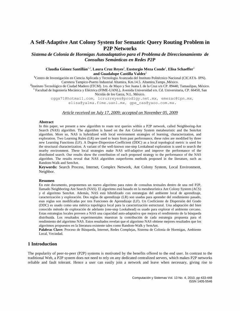
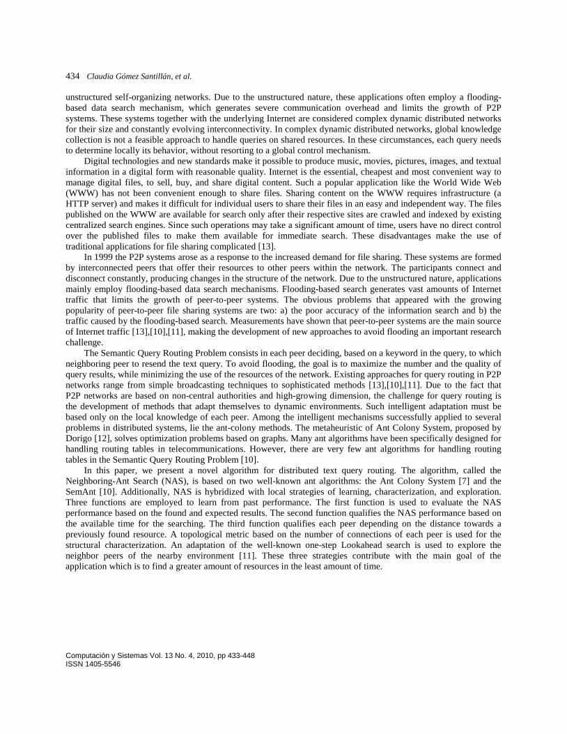
where resultsk represents the amount of results found by the ant k and maxResults is the amount of results requested. The value of the HIT function is applied in the global updating function, Eq. (8), with the purpose of guiding the queries toward routes that provide the greatest possible amount of found resources. This HIT value is registered in each node of the path traversed by the search ant, as shown in Figure 1. Importance of Time-to-live Function (ITL_HOP), qualifies the performance of the search agent k, based on the time-to-live used to find one resource (TTLk) and the maximum time-to-live originally assigned:
k
maxTTLITL_HOP =2×TTL
, ( 3 )
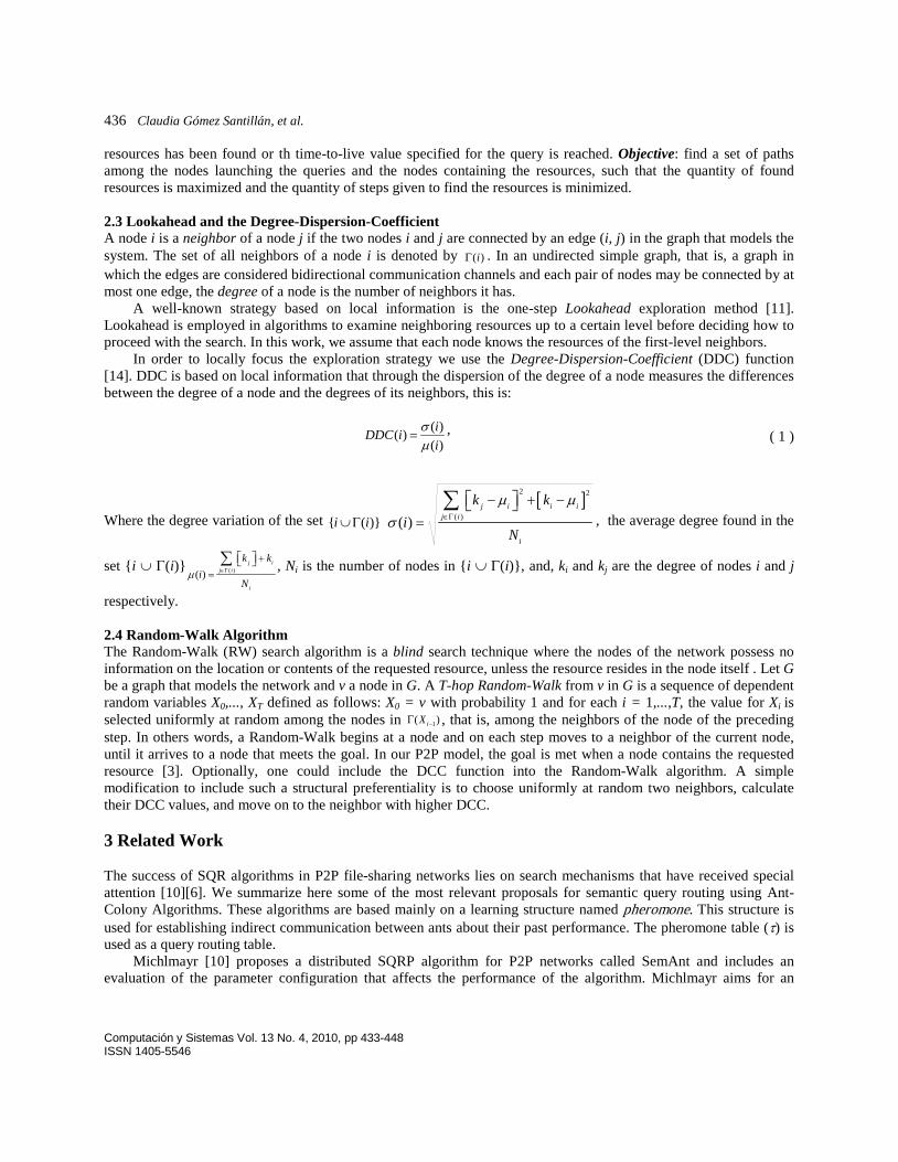
where TTLk is the partial time-to-live of the ant k until the moment, and maxTTL is the maximum time-to-live assigned to an ant for a query. These time measures are given in terms of the number of hops and correspond respectively with the given steps and the maximum steps allowed to each ant. The result is applied into the global updating rule, Eq. (8), with the overall goal of decreasing the time-to-live necessary to find a set of resources. The ITL_HOP value is registered in each node of the path traversed by the ant until the node with the last resource is found, as shown in Figure 2. Importance of Distance Function (ID_HOP), for the agent k, shown in Eq. (4), qualifies each node s, which is a neighbor of the current node r, depending on the distance towards a previously found resource t:
, of -1
kr,s,t
r,s,t
hID_HOP = r s route kh
∀ ∈
( 4 )
when r is the current node, s is the evaluated node, t is the found resource, k is the ant agent, hk is the total number of steps taken by the agent, and hr,s,t is the number of hops from the source to an evaluated resource node. Once an ant k generates a route to a resource t, the function ID_HOPr,s,t is applied to each node belonging to this route to increase its importance in terms of the distance to a found resource node with respect to the length of the route. This function is obtained through the inverse of the total number of hops hk made by the ant on the route to the resource found,
TTLk = 5 maxTTL= 25 ITL_HOP = 2.5
resultsk = 3 maxResults = 5 HIT = 0.6
Fig. 1. Example of the calculation of the HIT function
Fig. 2. Example of the calculation of the ITL_HOP function

A Self-Adaptive Ant Colony System for Semantic Query Routing Problem in P2P Networks 439
Computación y Sistemas Vol. 13 No. 4, 2010, pp 433-448 ISSN 1405-5546
divided by the relative number of hops hr,s,t from the source to the node evaluated s, which is a neighbor of the current node r, as is shown in Figure 3. 4.2 Classical Learning Rules (LR) This section describes the modifications made to the two classical learning rules, originally proposed by Dorigo [7] in the ACS algorithm. The first rule is called state transition; with this rule the next node to be visited is selected. The transition rule uses two strategies: exploitation and exploration. The second rule is called updating; with this rule the ant updates the nodes in the traversed path. The updating rule uses two strategies: local and global updating of the pheromone. All strategies are used to feedback the system on successful routes.
Fig. 3. Example of the calculation of the ID_HOP function
The modified state transition rule of NAS is formulated by Eqs. (5) and (6). This:
, , , , 00,arg max _ , if (exploitation)
, otherwise (biased exploration),n n nn r L t L r L tL n L DDC ID HOP q q
sS
βτ∀ ∈
⋅ + ≤ =
( 5 )
where r is the current node where the ant k is located, u belongs to the set of neighboring nodes of r, Vk is the set of nodes visited by the ant k, τ is the pheromone table, t is the searched resource, β is the parameter that determines the relative importance between the pheromone and the DDC with ID_HOP, q is a random number, and q0 determines the relative importance of exploitation versus exploration. In case that q ≤ q0, the exploitation strategy is selected: it selects a node that provides a greater amount of pheromone and better connectivity with smaller numbers of hops toward a resource. Otherwise the exploration strategy, Eq. (6), is selected:
, , , ,, , , ,
, , , ,( )
_( ),
_k
r u t u r u tr u t r u t
r i t i r i ti r i V
DDC ID HOPS f p p
DDC ID HOP
β
β
τ
τ∀ ∈Γ ∧ ∉
⋅ + = = ⋅ + ∑
, ( 6 )
where S selects a node applying a random selection function f based on the well-known roulette-wheel selection to favor nodes with higher connectivity, stronger pheromone trail, and a shorter distance to a requested resource. This exploration strategy stimulates the ants to search for new paths. Note that the pseudorandom variable is modified by the DDC topological metric and the ID_HOP learning function.
The ACS updating rule is composed of both local and global updating. Hence the modified updating rule in this work is given in Eqs. (7) and (8). The local update strategy of NAS is formulated by:
, , , , 0(1 )r s t r s tτ ρ τ ρ τ← − ⋅ + ⋅ , ( 7 )
hk = 5 hr,s,t= 1, for r=1 and s =2 hr,s,t= 3, for r=3 and s =4 ID_HOPr,s,t = 1/5, for r=1 and s =2 ID_HOPr,s,t = 3/5, for r=3 and s =4
440 Claudia Gómez Santillán, et al.
Computación y Sistemas Vol. 13 No. 4, 2010, pp 433-448 ISSN 1405-5546
where r is the current node where the ant k is located, s is the current neighboring node where the ant is going to move, t is the searched resource, τ is the pheromone table where the ant does the local updating, 0τ is the initialization value of the pheromone, and ρ is the local evaporation factor of the pheromone. Each time an ant decides to move towards a node by the state transition rule, some pheromone is deposited at each node that has been visited to establish a trend towards the most frequently visited nodes. On the other hand, the modified global update strategy, given by Eq. (8), is computed each time that a resource is found and is applied to each node belonging to the route that lead to the discovery of the resource:
[ ], , , ,(1 ) (1 ) _ , of r s t r s t w HIT w ITL HOP r s path kτ α τ α← − ⋅ + ⋅ ⋅ + − ⋅ ∀ ∈ , ( 8 )
whereα is the global evaporation factor of the pheromone, and w is a weight factor that controls the relative importance between the resource found (HIT function) and the time-to-live (ITL_HOP function). The amount of pheromone deposited depends on the quality of the solution obtained, the amount of resources found, and the time-to-live of the ant at time of discovery. 5 Multi-agent Architecture and Parallel Pseudocode In this section we describe the NAS algorithm for the Semantic Querying Routing Problem. We first present an agent-based architecture and then a parallel pseudocode.
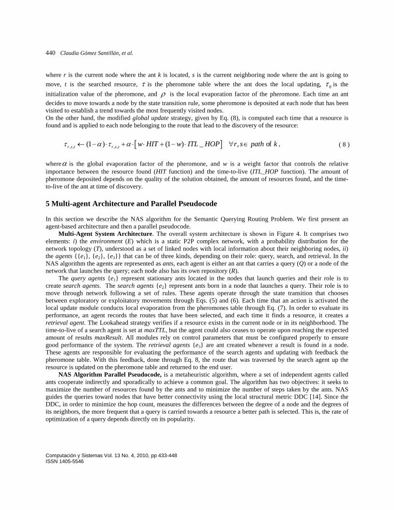
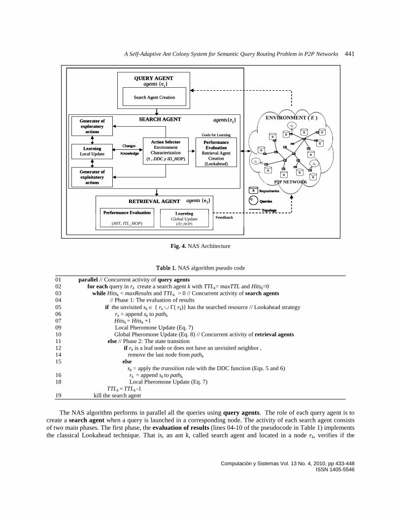
Multi-Agent System Architecture. The overall system architecture is shown in Figure 4. It comprises two elements: i) the environment (E) which is a static P2P complex network, with a probability distribution for the network topology (T), understood as a set of linked nodes with local information about their neighboring nodes, ii) the agents e1, e2, e3 that can be of three kinds, depending on their role: query, search, and retrieval. In the NAS algorithm the agents are represented as ants, each agent is either an ant that carries a query (Q) or a node of the network that launches the query; each node also has its own repository (R).
The query agents e1 represent stationary ants located in the nodes that launch queries and their role is to create search agents. The search agents e2 represent ants born in a node that launches a query. Their role is to move through network following a set of rules. These agents operate through the state transition that chooses between exploratory or exploitatory movements through Eqs. (5) and (6). Each time that an action is activated the local update module conducts local evaporation from the pheromones table through Eq. (7). In order to evaluate its performance, an agent records the routes that have been selected, and each time it finds a resource, it creates a retrieval agent. The Lookahead strategy verifies if a resource exists in the current node or in its neighborhood. The time-to-live of a search agent is set at maxTTL, but the agent could also ceases to operate upon reaching the expected amount of results maxResult. All modules rely on control parameters that must be configured properly to ensure good performance of the system. The retrieval agents e3 are ant created whenever a result is found in a node. These agents are responsible for evaluating the performance of the search agents and updating with feedback the pheromone table. With this feedback, done through Eq. 8, the route that was traversed by the search agent up the resource is updated on the pheromone table and returned to the end user.
NAS Algorithm Parallel Pseudocode, is a metaheuristic algorithm, where a set of independent agents called ants cooperate indirectly and sporadically to achieve a common goal. The algorithm has two objectives: it seeks to maximize the number of resources found by the ants and to minimize the number of steps taken by the ants. NAS guides the queries toward nodes that have better connectivity using the local structural metric DDC [14]. Since the DDC, in order to minimize the hop count, measures the differences between the degree of a node and the degrees of its neighbors, the more frequent that a query is carried towards a resource a better path is selected. This is, the rate of optimization of a query depends directly on its popularity.
A Self-Adaptive Ant Colony System for Semantic Query Routing Problem in P2P Networks 441
Computación y Sistemas Vol. 13 No. 4, 2010, pp 433-448 ISSN 1405-5546
Fig. 4. NAS Architecture
Table 1. NAS algorithm pseudo code
01 parallel // Concurrent activity of query agents 02 for each query in rk create a search agent k with TTLk= maxTTL and Hitsk=0 03 while Hitsk < maxResults and TTLk > 0 // Concurrent activity of search agents 04 // Phase 1: The evaluation of results 05 if the unvisited sk ∈ rk ∪ Γ( rk) has the searched resource // Lookahead strategy 06 rk = append sk to pathk 07 Hitsk = Hitsk +1 09 Local Pheromone Update (Eq. 7) 10 Global Pheromone Update (Eq. 8) // Concurrent activity of retrieval agents 11 else // Phase 2: The state transition 12 if rk is a leaf node or does not have an unvisited neighbor , 14 remove the last node from pathk 15 else sk = apply the transition rule with the DDC function (Eqs. 5 and 6) 16 rk = append sk to pathk 18 Local Pheromone Update (Eq. 7) TTLk = TTLk -1 19 kill the search agent
The NAS algorithm performs in parallel all the queries using query agents. The role of each query agent is to
create a search agent when a query is launched in a corresponding node. The activity of each search agent consists of two main phases. The first phase, the evaluation of results (lines 04-10 of the pseudocode in Table 1) implements the classical Lookahead technique. That is, an ant k, called search agent and located in a node rk, verifies if the
ENVIRONMENT ( E )
P2P NETWORK
SEARCH AGENT
Performance Evaluation
Retrieval Agent Creation
(Lookahead)
Action SelectorEnvironment
Characterization(τ , DDC y ID_HOP)
LearningLocal Update
Changes
Knowledge
Generator ofexploitatory
actions
Goals for Learning
Generator ofexploratory
actions
LearningGlobal Update
(ID_HOP)
Performance Evaluation
(HIT, ITL_HOP)
RETRIEVAL AGENT
Feedback
QUERY AGENT
Search Agent Creation
agents e1
agentse2
agents e3Q
R Repositories
Queries
Topology
R
R
R
R
RR
R
R
RR
R
Q2Q1
Q3
ENVIRONMENT ( E )
P2P NETWORK
SEARCH AGENT
Performance Evaluation
Retrieval Agent Creation
(Lookahead)
Action SelectorEnvironment
Characterization(τ , DDC y ID_HOP)
LearningLocal Update
Changes
Knowledge
Changes
Knowledge
Generator ofexploitatory
actions
Goals for Learning
Generator ofexploratory
actions
LearningGlobal Update
(ID_HOP)
Performance Evaluation
(HIT, ITL_HOP)
RETRIEVAL AGENT
Feedback
QUERY AGENT
Search Agent Creation
agents e1
agentse2
agents e3Q
R Repositories
Queries
Topology
R Repositories
Queries
Topology
R
R
R
R
RR
R
R
RR
R
Q2Q1
Q3
442 Claudia Gómez Santillán, et al.
Computación y Sistemas Vol. 13 No. 4, 2010, pp 433-448 ISSN 1405-5546
resource exists in an unvisited node sk that belongs to its neighborhood, including itself. If the resource is found, the ant adds the node sk to its path, updates the number of occurrences of the queried resource Hitsk, reduces the ant time TTLk by one hop, performs the local pheromone update according to Eq. (7), and performs the global pheromone update according to Eq. (8). The global updating of the pheromone is a concurrent activity of the ants called retrieval agents; the route to the resource is updated on the pheromone table and returned to the end user. In the case that the evaluation phase fails, a second phase, the state transition (lines 11-18 of the pseudocode in Table 1) is carried out. This phase selects through random number q, Eq. (5), a neighbor node s. In the case that there is no new node towards which to move, that is to say, the node is a leaf or all neighbor nodes have been visited, a hop backwards is carried out on the path. Otherwise the ant adds the selected node sk to its path, updates locally the pheromone, Eq. (7), and reduces TTLk by one hop. The query process ends when the expected number of results has been found or TTLk reaches zero. In both cases the search agent is killed, indicating the end of the query. 6 Experimental Analysis of the NAS Algorithm In this section, we describe two experiments carried out on the NAS algorithm. The objective of the first experiment is study the performance of NAS in comparison with algorithms proposed in the literature, SemAnt and Random-Walk. The objective of the second experiment is to examine the contribution of each local environment strategy to the performance of the NAS algorithm.
6.1 Experiments Setup The NAS algorithm was implemented to solve SQRP instances. The application of the NAS algorithm requires the specification of the problem instance to solve and the definition of the control parameters of the algorithm. In our implementation, an SQRP instance is determinated by three separate files: topology, repositories, and queries. We generated the experimental instances as follows.
The generation of the topology (T) is based on the method of Barabási et al. [4] to create a non-uniform network with a scale-free distribution. In the scale-free or power law distribution, a reduced set of nodes has a very high degree and the rest of the nodes have a small degree. All networks generated have 1,024 nodes and bi-directional edges. The number of nodes was selected based on recommendations by Michlmayr [10] and Di Caro [6].
In the P2P model, each peer manages a local repository (R) of resources and offers its resources to other peers. We generated these repositories using “topics” obtained from ACM Computing Classification System taxonomy (ACMCCS). This database contains a total of 910 distinct topics. Also the content distribution is a power law: few nodes contain many topics in their repositories and the rest of the nodes contain few topics.
For the generation of the queries (Q), each node was assigned a list of possible topics to search. This list is limited by the total amount of topics of the ACMCCS. During each step of the experiment, each node has a probability of 0.1 to launch a query, selecting the topic uniformly at random within the list of possible topics of the node. The probability distribution of Q determines how often the query will be repeated in the network. When the distribution is uniform, each query is duplicated 100 times on average.
The topology and the repositories were created static, whereas the queries were launched randomly during the simulation. Each simulation was run for 20,000 time units (queries). The average performance was studied by computing three performance measures each 100 units of time: Average hops, defined as the average amount of links travelled by a search agent until its death (that is, reaching either maxResults = 10 or maxTTL = 25). Average hit-rate, defined as the average number of resources found by each search agent until its death and Average efficiency, defined as the average hit-rate divided by the average hops.
The control parameters of the algorithm are specified in a file containing a global static configuration of the NAS algorithm parameters. The configuration of the NAS algorithm used in the experimentation is shown in Table 2. In the first column is the parameter value and the in second column is given a description of the parameter. These parameter values were based on recommendations done by Michlmayr [10] and Dorigo [7].

A Self-Adaptive Ant Colony System for Semantic Query Routing Problem in P2P Networks 443
Computación y Sistemas Vol. 13 No. 4, 2010, pp 433-448 ISSN 1405-5546
6.2 Comparative study of the NAS algorithm In this experiment, the performance of the NAS algorithm is compared against the SemAnt [10] and Random-Walk [3] algorithms. For the experimentation with three algorithms we use the general specifications described in Section 6.1.
To carry out the experiment with the SemAnt algorithm with the same conditions, we only changed the parameter number of links. For SemAnt [10], the number of connections range between 4,000 and 10,000 which does not affect the performance of the algorithm. Hence, we fixed the number of the links to 7,000 links, choosing an intermediate value in that range.
Table 2. Configuration parameter of the NAS algorithm
Parameter Definition ρ= 0.07 Local pheromone evaporation factor α= 0.07 Global pheromone evaporation factor τ0 = 0.009 Pheromone table initialization ID_HOP0 = 0.001 Initial value of the table of distances to previously encountered resources β = 2 Relative importance of DDC and ID_HOP with respect to the pheromone q0 = 0.9 Relative importance between exploration and exploitation maxResults =10 Maximum number of results to retrieve maxTTL = 15 Time-to-live of the search agents w = 0.5 Relative importance of the resources found and the time-to-live
The experimental values for the SemAnt algorithm were obtained from [10]. For the average hit-rate variable
the SemAnt algorithm shows values from 0.8 to 2.1 hits per query. However, for the NAS algorithm, the average hit-rate ranges from 9.5 to 10 hits per query. On the other hand, the average hop count of the SemAnt algorithm starts out at 23 and lowers to 16 hops per query during the operation of the algorithm, whereas the NAS algorithm, starts at the average hop of 12.5 and then diminishing to 12 hops per query. Finally, the average efficiency of the SemAnt algorithm improves from 0.034 to 0.13 hits per hop, while for the NAS algorithm, as shown in Figure 5, it increases from an initial value of 0.76 up to 0.84 hits per hop.
Fig. 5. Performance of NAS Algorithm average efficiency
For the experiment with the Random-Walk (RW) algorithm, we also used the general specifications described in
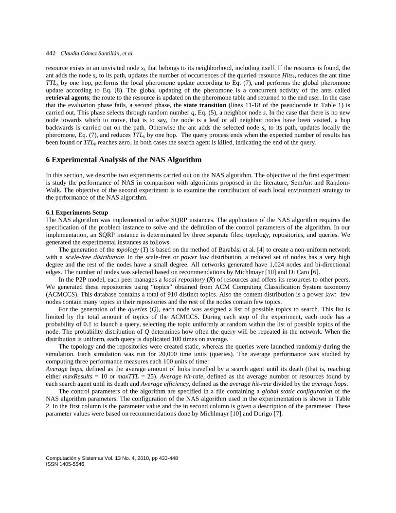
Section 6.1. Figure 6(a) shows the average hit-rate for both RW and NAS algorithms. The behavior changes slightly over time. That is, the average hit-rate in RW varies between 1 to 0.5 hits per query, while in NAS, the average hit-rate varies between 9.6 to 10 hits per query. Similarly Figure 6(b) shows the average hop count for both RW and
444 Claudia Gómez Santillán, et al.
Computación y Sistemas Vol. 13 No. 4, 2010, pp 433-448 ISSN 1405-5546
NAS algorithms. The behavior of the RW does not evolve; the average hop count keeps around 15 hops per query, from the beginning to the end. However in NAS the behavior evolves, starting at 12.5 and lowering down to 12 hops on average. Finally, Figure 6(c) shows the average efficiency for both RW and NAS algorithms. In the RW algorithm, the behavior does not evolve; the average efficiency keeps around 0.5 hits per hop. For NAS the behavior does evolve; so that the average efficiency increases from 0.76 to 0.84 hits per hop.
Fig. 6. Comparison of NAS Algorithm against Random-Walk Algorithm. a) average hits-rate,
b) Average hops and c) average efficiency
A Self-Adaptive Ant Colony System for Semantic Query Routing Problem in P2P Networks 445
Computación y Sistemas Vol. 13 No. 4, 2010, pp 433-448 ISSN 1405-5546
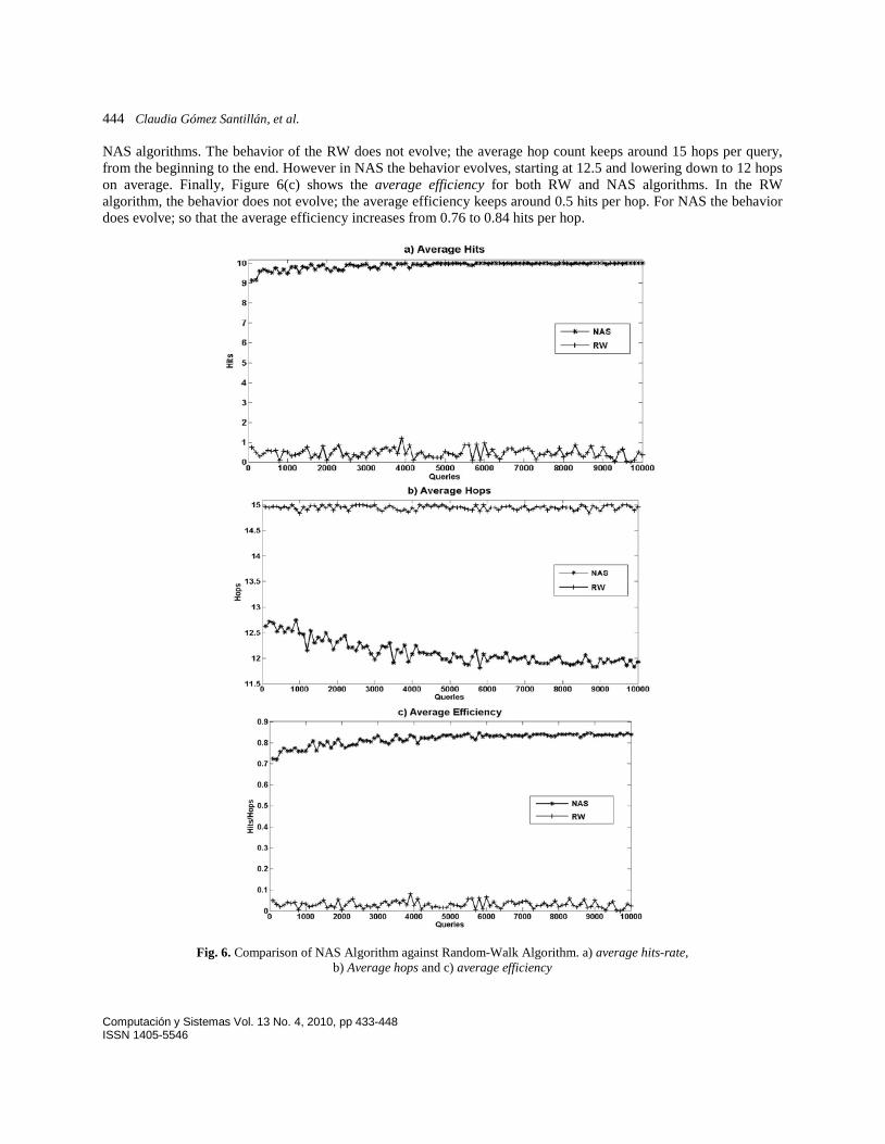
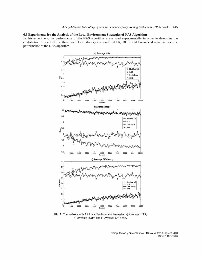
6.3 Experiments for the Analysis of the Local Environment Strategies of NAS Algorithm In this experiment, the performance of the NAS algorithm is analyzed experimentally in order to determine the contribution of each of the three used local strategies – modified LR, DDC, and Lookahead – to increase the performance of the NAS algorithm.
Fig. 7. Comparisons of NAS Local Environment Strategies. a) Average HITS,
b) Average HOPS and c) Average Efficiency
446 Claudia Gómez Santillán, et al.
Computación y Sistemas Vol. 13 No. 4, 2010, pp 433-448 ISSN 1405-5546
For evaluating the contribution of modified LR, DDC and Lookahead strategies were eliminated. The contribution of DDC was evaluated eliminating only Lookahead; modified LR was kept because DDC is included in it. Similarly, Lookahead was evaluated without modified LR and DDC. For the experiment with the NAS algorithm, we used the general specification described in Section 6.1, with the exception of three parameters: maxResult =5, maxTTL=10, and q0 = 0.90.
Figure 7(a) shows the average hit-rate performed during a set of queries with NAS and three different configurations of NAS: modified LR, DDC and Lookahead. For the modified LR and DDC, the algorithms start approximately at 0.5 hits per query; at the end, the average hit-rate increases to 2 hits per query. For Lookahead and NAS the average hit-rate starts at 4.3 and after 1,000 queries the behavior changes; for Lookahead the average hit-rate ends at 4 and for NAS ends at 5. On the other hand, Figure 7(b) shows the average hops performed during in a set of queries with NAS and three different configurations. For modified LR and DDC, the behavior is approximately the same; the average hop count starts at 10 and ends at 9.5 hops per query. However, the Lookahead and NAS start at 7.8 and after 1500 queries, the behavior changes; for Lookahead the average hop count ends at 8 and for NAS ends at 6.9 hops per query. Finally, Figure 7(c) shows the average efficiency. For the modified LR and DDC, the behavior is approximately the same; at the beginning the efficiency is around 0.05, at the end the efficiency increases to 0.2 hits per hop. However, for the Lookahead and NAS, the behavior evolves such that the average efficiency stars at 0.55 and after 1,500 queries, the behavior changes; for Lookahead, the average efficiency ends at 0.5, for NAS, the average efficiency ends at 0.7. Hence, the best performance was obtained with the combination of these three strategies.
Besides, the results reveal that for the specified configuration, the Lookahead method shown the biggest contribution to the final performance of NAS, giving an efficiency of 0.5 hits per hop. While the DDC and modified LR had a similar impact of 0.2 hits per hop. In experimentations with other configurations [13], the analyzed strategies have shown different contributions. Due to this result, it becomes relevant to study further the relations that exist between the problem characteristic and the algorithm parameter configuration in order to yield a bigger benefit of each one local strategy proposed for NAS. 7 Conclusions and future work
For the solution of the Semantic Query Routing Problem (SQRP), we proposed a novel algorithm called NAS that is based on existing ant colony algorithms but incorporating local environment strategies: modified LR, DDC, and Lookahead. Three functions are used to learn from past performance: importance of hits (HIT), importance of time-to-live (ITL_HOP), and importance of distance (ID_HOP). This combination results in a lower hop count and an upper hit count, outperforming two algorithms proposed in related work, Random-Walk and SemAnt.
Our analysis and simulations confirm that the proposed techniques are more effective at improving search efficiency. Specifically the NAS algorithm in the efficiency shows six times better performance efficiency, than the SemAnt, and seventeen times better performance than the Random-Walk. We observe that upon including learning and characterization with modified LR and DDC respectively, the algorithm evolves to reach an average of 2 hits with 9.5 hops per query. Adding only exploration with Lookahead, the algorithm keeps a constant performance of 4 hits with 8 hops. Combining all the three strategies the NAS algorithm evolves to yield 5 hits per 6.9 hops. As observed, the best results were obtained in the combination of proposed strategies.
We plan to study more profoundly the relation among SQRP characteristics, the configuration of NAS algorithm and the local environment strategies employed in the learning curve of ant-colony algorithms, as well as their effect on the performance of hop and hit count measures. References 1. Amaral, L. A. N., & Ottino, J. M. (2004). Complex Systems and Networks: Challenges and Opportunities for
Chemical and Biological Engineers, Chemical Engineering Scientist, 59(1), 1653–1666.

A Self-Adaptive Ant Colony System for Semantic Query Routing Problem in P2P Networks 447
Computación y Sistemas Vol. 13 No. 4, 2010, pp 433-448 ISSN 1405-5546
2. Androutsellis-Theotokis Stephanos & Diomidis Spinellis (2004). A Survey of Peer-to-Peer Content Distribution Technologies. ACM Computing Surveys, 36(4), 335–371.
3. Arora, S., & Barak, B. (2009). Complexity Theory: A Modern Approach. New York: Cambridge University Press.
4. Barabasi, A., Albert & R., Jeong, H. (1999). Mean-Field theory for Scale-free Random Networks. Physical A, 272(1), 173–189.
5. Cruz-Reyes, L., Gómez S. C., Aguirre L. M., Schaeffer E., Turrubiates L.T., Ortega I. R., & Fraire H. H. (2008). NAS Algorithm for Semantic Query Routing System for Complex Network. International Symposium on Distributed Computing and Artificial Intelligence 2008 (DCAI 2008), Advances in Soft Computing, 50, 284-292.
6. Di Caro, G. & Dorigo, M. (1998). AntNet: Distributed Stigmergy Control for Communications Networks. Journal of Artificial Intelligence Research, 9(1), 317-365.
7. Dorigo, M. & Gambardella, L. M. (1997). Ant Colony System: A Cooperative Learning Approach to the Traveling Salesman Problem, IEEE Transactions on Evolutionary Computation, 1(1), 53-66.
8. Erdős, P. & Rényi, A. (1960). On the Evolution of Random Graphs. Publications of the Mathematical Institute of the Hungarian Academic of Sciences. 5(1), 17-61.
9. Liu, J., XiaoLong, J. & Kwok, C.T. (2005). Autonomy Oriented Computing /From Problem Solving to Complex System Modeling. New York: Kluwer Academic Publisher.
10. Michlmayr, E. (2007). Ant Algorithms for Self-Organization in Social Networks. PhD Thesis, Vienna University of Technology. Austria, Vienna.
11. Mihail, M., Saberi A. & Tetali P. (2006). Random Walks with Lookahead in Power Law Random graphs. Internet Mathematics, 3(2), 147-152.
12. Ortega R., Meza E., Gómez C., Cruz L., & Turrubiates T. (2007). Impact of Dynamic Growing on the Internet Degree Distribution. Polish Journal of Environmental Studies, 16(1), 117-120.
13. Sakaryan G. (2004). A Content-Oriented Approach to Topology Evolution and Search in Peer-to-Peer Systems, PhD Thesis, University of Rostock. Rostock, Germany.
14. Yang, K. & Wu, C., Ho, J. (2006). AntSearch: An Ant Search Algorithm in Unstructured Peer-to-Peer Networks. IEICE Transactions on Communications, 89(9), 2300-2308.
Claudia Gómez S. was born in Mexico in 1971. She is a doctoral student at National Polytechnic Institute, Mexico. She received her MS degree in Computer Science from the Leon Institute of Technology, Mexico, in 2000. Her research interests are optimization Techniques, complex network and autonomous agents.
Laura Cruz-Reyes was born in Mexico in 1959. She received the PhD (Computer Science) degree from National Center of Research and Technological Development, Mexico, in 2004. She is a professor at Madero City Institute of Technology, Mexico. Her research interests include optimization techniques, complex networks, autonomous agents and algorithm performance explanation.

448 Claudia Gómez Santillán, et al.
Computación y Sistemas Vol. 13 No. 4, 2010, pp 433-448 ISSN 1405-5546
Eustorgio Meza received the PhD (Oceanic Engineering) deegree from Texas A&M University, College Station, U.S.A. He received the MS degree in Computer Science (AI) from Institute of Technology and Advanced Studies of Monterrey, Mexico. He is a Professor at Research Center in Applied Science and Advanced Technology from National Polytechnic Institute. His research interests are oceanology, complex Network.
Elisa Schaeffer was born in Finland in 1976. She received the PhD (Science in Technology) degree from Helsinki University of Technology, Finland, in 2006. She is a teaching researcher at the Graduate Program in Systems Engineering (PISIS), at the Faculty of Mechanical and Electrical Engineering (FIME), Universidad Autonoma de Nuevo Leon, Mexico. Her research interests include nonuniform networks, graph clustering and optimization of network operation
Guadalupe Castilla. is a doctoral student at Madero Institute of Technology, Mexico. She received her MS degree in Computer Science from the Leon Institute of Technology, Mexico, in 2002. Her research interests are optimization Techniques.
Accepted Manuscript
Ant colony system with characterization-based Heuristics for abottled-products distribution logistics system
Claudia G. Gomez S., Laura Cruz-Reyes, Juan J. Gonzalez B., HectorFraire H., Rodolfo A. Pazos R., Juan J. Martınez P.
PII: S0377-0427(13)00588-8DOI: http://dx.doi.org/10.1016/j.cam.2013.10.035Reference: CAM 9429
To appear in: Journal of Computational and AppliedMathematics
Received date: 15 February 2013Revised date: 18 October 2013
Please cite this article as: C.G. Gomez S., L. Cruz-Reyes, J.J. Gonzalez B., H. Fraire H., R.A.Pazos R., J.J. Martınez P., Ant colony system with characterization-based Heuristics for abottled-products distribution logistics system, Journal of Computational and AppliedMathematics (2013), http://dx.doi.org/10.1016/j.cam.2013.10.035
This is a PDF file of an unedited manuscript that has been accepted for publication. As aservice to our customers we are providing this early version of the manuscript. The manuscriptwill undergo copyediting, typesetting, and review of the resulting proof before it is published inits final form. Please note that during the production process errors may be discovered whichcould affect the content, and all legal disclaimers that apply to the journal pertain.
Ant Colony System with Characterization-Based
Heuristics for a Bottled-Products Distribution
Logistics System
Claudia G. Gómez S., Laura Cruz-Reyes, Juan J. González B., HéctorFraire H., Rodolfo A. Pazos R., Juan J. Martínez P.
Instituto Tecnológico de Ciudad Madero, Av. 1o. de Mayo s/No Col. Los Mangos, Cd.Madero, Tamaulipas, Mexico.
Abstract
The aim of this paper is to show the solution of the Vehicle Routing Problemwith Time Windows (VRPTW) as a key factor to solve a logistics systemfor the distribution of bottled products. We made a hybridization betweenan Ant Colony System algorithm (ACS) and a set of heuristics focused oninstance characterization and performance learning. We mainly propose amethod to make a constrained list of candidate customers called ExtendedConstrained List (ECL) heuristics. Such list is built based on the character-ization of the time-window and the geographical distribution of customers.This list gives priority to the nearest customers with a smaller time window.The ECL heuristics is complemented by the Learning Levels (LL) heuris-tics, that allows the ants to use the pheromone matrix in two phases: localand global. In order to validate the benefits of each heuristics, a series ofcomputational experiments were conducted using the standard Solomon’sbenchmark. The experimental results show that, when the ECL heuristics isincorporated in the basic ACS algorithm, the number of required vehicles isreduced by 28.16%. When the LL heuristics is incorporated, this reductionincreases to 36.83%. The experimentation reveals that, by a suitable char-acterization, preexisting conditions in the instances are identified in order totake advantage from both of the ECL and LL.
Keywords: Heuristics hybridization, Vehicle routing problem, Ant colonysystem algorithm.
Preprint submitted to Journal of Computational and Applied MathematicsOctober 18, 2013
ManuscriptClick here to view linked References
1. Introduction
Logistics systems applied to transport systems are a current problem inproductive and service sectors. Distributors should effectively and efficientlystock customers with products, which constitutes a major challenge for a lo-gistics system, since resources are limited and transportation costs constitutea high percentage of the value added to goods: from 5% to 20% [1]. Solvingreal-life world transportation problems requires the development of robustmethods that support the complexity of these kind of problems. In orderto contribute to this area, we have a methodological solution developed byintegrating the main tasks (routing, scheduling and loading) involved in ageneric transportation problem, called RoSLoP [2, 3].
RoSLoP focuses mainly on routing vehicles applied to the distributionof bottled products in a company located in northeast Mexico [2, 6]. Theobjective of the routing task is to define routes for vehicles so as to minimiz-ing the total cost subject to twelve real world constraints [2]. Consideringthe difficulty of handling several realistic constraints at the same time, thisproblem is often called Rich VRP [4, 3].
This work extends the solution presented in [2] for RoSLoP, particularlyfor the VRPTW routing task. The proposal of this research is based on aheuristics hybridization of an ACS algorithm. The purpose of the hybridiza-tion is to improve the optimization process by characterizing the problemaccording to two aspects of customers: geographic distribution (topology)and service time distribution (time-window types). The heuristics are: Ex-tended Constrained List (ECL) and Learning Levels (LL) [5, 3]. The firstheuristics constitutes the main contribution of this work, it provides a higherprobability of selection of those customers which are closer and have smallertime-window types, whereas the second heuristics slightly increases the prob-ability for movements which have previously contributed to improve the so-lution.
Like our work, researchers have presented since the 1960’s their proposalsrelated to VRPTW in order to solve this problem. The main work includesPisinger and Ropke [7], who present an extension of Large NeighborhoodSearch (LNS) proposed by [8]. Their algorithm, called ALNS, is an adapta-tion of the LNS algorithm by building partial neighborhoods which competeto iteratively modify the current solution.
Another researcher, Mester [9], proposed a heuristic algorithm based on(1+1) multi-parametric evolutionary strategies. Three operators are used for
2
the removal of customers (purely random removals, removal of one customerfrom each route, and random ejections from rings generated from two cir-cles centered on the depot with random radiuses), while a cheapest insertionheuristics is applied for re-insertion. Each offspring is further improved us-ing Or-Opt, Exchange, 2-Opt local moves within a parameterized dynamicenvironment “Adaptive Variable Neighborhood” (AVN). In an effort to prunethe neighborhood space, a strategy for selecting neighboring routes, called“Dichotomous Route Combinations” (DRC), is also used to take advantageof the geographical division and topology of the vehicle routes.
A different strategy, but also based on Local Search, is proposed byPrescott-Gagnon et al. [10]; they present a hybridization of a branch-and-price heuristic technique, a LNS method composed by operators related tocustomer selection known as: Proximity, SMART, and Longest Detour. An-other local-search based heuristics was developed by Hoshino et al. [11];such heuristics is controlled by chaotic dynamics exploiting principles of neu-ral networks. The chaotic search applies by exchanging and relocating localmoves. The neurons are updated asynchronously while a single iterationis performed, and finally the route elimination heuristics of [12] is appliedperiodically for further improvement.
After reviewing state-of-the-art papers, it is concluded that the ECL andLL heuristics are original. Table 4 in Subsection 5 presents comparativeresults obtained by our ACS algorithm including the proposed heuristicsversus other works here presented.
2. Vehicle Routing Problem with Time Windows (VRPTW)
Vehicle routing has been of great interest for the scientific community overthe past fifty years. However, open questions remain due to its complexity[13]. VRP, defined by Dantzig in [14], is a classic combinatorial optimizationproblem. It consists of trying to service a set of customers using a fleet ofvehicles, respecting constraints on the vehicles, customers, drivers, and soon. Among the most important variants of VRP is the VRPTW defined byKallehauge in [15]. This problem consists of finding the optimal routing of afleet of vehicles from a depot to a number of customers that must be visitedwithin a specified time interval, called time window. A time and capacityconstrained digraph G = (V,A, c, t, a, b, d, q) is defined with the followingelements:
3

• a node set V = V∗ ∪ 0, n + 1, where V∗ = 1, . . . , n is the set ofcustomer nodes, and the nodes 0 and n+ 1 are the starting depot andthe returning depot respectively,
• an arc set A = A∗ ∪ δ+(0) ∪ δ−(n + 1), where A∗ = A(V∗), is the setof arcs (i, j) such that (i, j) ∈ V∗, additionally δ+ (0) = (0, i)|i ∈ V∗is the set of arcs leaving the start depot node, and δ− (n + 1) = (i,n+ 1)|i ∈ V∗ is the set of arcs entering the destination depot node,
• durations (traveling time) on arcs t ∈ N|A|, such that tij ≤ tik + tkj , fori, j, k ∈ V,
• start and end service time on nodes a, b ∈ Z+ ∪ +∞|V |, wherea0 = an+1 = 0, b0 = bn+1 = +∞, ai ≥ t0i, bi ≥ ai for i ∈ V∗ andbj ≥ ai + tij for (i, j) ∈ A∗,
• demands on nodes d ∈ Z|V |+ , where d0 = dn+1 = 0,
• and a vehicle capacity q ∈ Z+ where q ≥ di for i ∈ V∗ and q ≥ di + dj
for (i, j) ∈ A∗.
For any path P = (v1, . . . , vk) in G, the arrival times of the set of nodes
V (P ) of the path is the vector s ∈ Z|V (P )|+ , whose elements are defined as
follows: sv1 = av1 , and svi= maxi=2,...,ksvi−1
+ tvi−1vi, avi. The demand of
the path is d(V (P )).A path P = (v1, . . . , vk) in G is feasible if svi
≤ bvifor i ∈ V (P ) and
d(V (P )) ≤ q. A feasible route R from 0 to n + 1 in G is defined as R =(0, v2, . . . , vk−1, n + 1). We denote by ℜ the set of all feasible routes from0 to n + 1 in G. For each feasible route a vehicle is required to service thecustomers included in the route.
Given a time and capacity constrained digraph G, the vehicle routingproblem with time windows consists of minimizing the number of requiredvehicles and the total time required to service all the customers demand.
As VRPTW is a multiobjective problem, in this work a hierarchical tech-nique is applied; i.e., the objectives of the problem are achieved consecutively:minimizing the number of vehicles required, and minimizing the traveling andwaiting times required to service all customers.
3. Hybridization of the Ant Colony System Algorithm
Ant algorithms were inspired by the behavior of ants in search for food,because in performing the search, each ant drops a chemical called pheromone,
4

which provides an indirect communication among the ants. Every algorithmbased on ant colony includes two main features: a heuristic measure ηij ,which provides information related to the problem used to compute pref-erence of travel; a larger ηij value implies a larger probability of selectingnode j. The second feature is trails of artificial pheromone τij , which is atable that keeps learning over time and is used in the selection rule of thenext customer to visit [16]. These heuristic measures are included within theACS − VEI() and ACS − TIME() functions and are explained in Subsection4.3.
To build feasible solutions for RoSLoP, three modules were created: rout-ing, scheduling and loading. The routing module is an Ant Colony Systemalgorithm [2]. The first action of Algorithm 1 consists of applying the Ex-tended Constrained List (ECL) heuristics, which aims at characterizing thetopology and time windows (see construction details in Subsections 4.1 and4.2). Next, an initial solution is calculated, using the nearest-neighbors strat-egy [18].
Algorithm 1 ACS algorithm for RoSLoP routingMultiple Ant Colony System (ρ, β, q0)ECL() / ∗ Construction of the constrained listψgs ← InitialSolution()repeat
vehicles← active_vehicle(ψgs)/∗ Number of vehicles used by the best solutionvehiclesbeta← vehicles− 1//begin ACS − VEI/∗ vehicle minimization process
LL (ψls)LocalSearch (ψls)textbfif (ψlsisfeasible)ψgs = ψls
end if
until stop criterion is satisfiedrepeat
ψls ← ψgs
//begin ACS − TIME/∗ vehicle minimization processLL (ψls)LocalSearch (ψls)if (ψls < ψgs)ψgs = ψls
end if
until stop criterion is satisfied
In the following lines Algorithm 1 creates two ant colonies: the first for
5
minimizing the number of vehicles and the second for minimizing travel time.Each colony is constituted by a set of ants and each step builds a localsolution (ψls), which will be evaluated to identify the best local solution(ψls); therefore, it is considered as the global solution (ψgs). The value of thepheromone is modified to stimulate finding both popular and better routes.At each step, the result from the ECL heuristics is used to select the nextcustomer to be visited, which favors choosing the nearest customers andthose that have limited opening hours (see details in Subsection 4.3). TheLearning Levels (LL) heuristics takes control of the pheromone on two levels:the lowest level is for each ant and the highest for each colony [5, 3] (seedetails in Subsection 4.4).
4. Heuristics for selecting customers
This section describes two heuristic methods proposed to build a customerlist grouped by proximity and availability of service, another heuristics keepsa table with information from the best solutions so far obtained. Their aimis to limit the selection of customers to those with characteristics suitablefor the route under construction. These heuristics collaborate hybridizingAlgorithm 1 to improve its performance.
4.1. Construction of the constrained list using topological characterization
The first part of the heuristic method, proposed for customer selection,is based on a clustering technique. A list of clusters of candidates is gener-ated considering feasibility conditions and the location of the customers inthe graph. Particularly, a clustering technique based on topological charac-terization is applied to limit the global population into subsets that fulfillfeasibility and closeness. The use of this clustering technique by the antsin the constructive process is very advantageous; while the hybridizationreduces the search space in the creation of feasible solutions due to the incor-poration of instance information about the distribution of the customers andthe depot. The constrained list organized by clusters is created as follows:
1. A minimum spanning tree T is generated including all the customersand the depot of the instance with Algorithm 2. This tree T is a sub-graph of A that connects all customers at minimal cost. Figure 1 showsthe result of calculating T for some Solomon’s instances [17].
6

Algorithm 2 Construction of the Minimun Spanning Tree TT = ∅, L = A, Sort(L)for each (i, j) ∈ L
if i and j belong to Tdiscard(i, j)
else
T = T ∪ (i, j)
0
10
20
30
40
50
60
70
80
90
0 10 20 30 40 50 60 70 80 90 100
Y
X
MINIMUM SPANNING TREE - type C
0
10
20
30
40
50
60
70
80
0 10 20 30 40 50 60 70
Y
X
MINIMUM SPANNING TREE - type R
0
10
20
30
40
50
60
70
80
90
0 10 20 30 40 50 60 70 80 90 100
Y
X
MINIMUM SPANNING TREE - type RC
Figure 1: Example of a T for each type of instance: C, R and RC
7
2. Parameters µ and σ are calculated from expressions (1) and (2), whereeach tcij is the distance from customer i to customer j. These data willbe used for defining the percentage of variability.
µ =∑
i,j ǫT, i 6=j
tcij (1)
σ =
√1
|V |∑
i,jǫ T
(tcij − µ)2 (2)
3. The percentage of variability θ of the associated costs of each arc be-longing to T is computed by expression (3), notice that θ normalizesσ.
θ =σ
2(max(i,j)∈Ttcij −min(i,j)∈Ttcij)(3)
In case θ < 0.1 (very small variability), the location of the customersin the instance approaches a uniform distribution; therefore, the entirepopulation forms a single cluster. Otherwise, a value of θ ≥ 0.1 revealsthe possible existence of regions with different density.
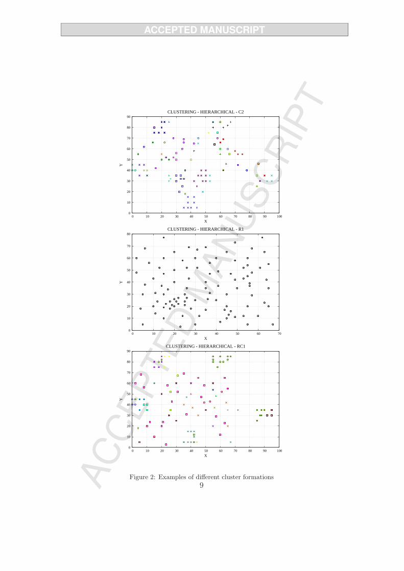
4. The formation of the set of clusters H is carried out by performing ahierarchical clustering when the rule “if θ ≥ 0.1” is satisfied; otherwise,customers form a single cluster |H| = 1. Figure 2 shows clusters formedunder variability percentage as defined by expression (3).
5. In the proposed hierarchical clustering, each customer starts in its owncluster, and pairs of clusters are merged iteratively in order to find anappropriate set of clusters H , based on an acceptance threshold ω. Theinitial value for ω is calculated by expression (4).
ω = 2 max(i,j)∈Ttcij (4)
For each pair of clusters (hi, hj), where hi, hj ∈ H , the well knowMahalanobis Distance (dM) is used with the rule “if dM(hi, hj) < ωand hi 6= hj then hi ∪ hj” for determining if both clusters are mergedin one cluster.
8
0
10
20
30
40
50
60
70
80
90
0 10 20 30 40 50 60 70 80 90 100
Y
X
CLUSTERING - HIERARCHICAL - C2
0
10
20
30
40
50
60
70
80
0 10 20 30 40 50 60 70
Y
X
CLUSTERING - HIERARCHICAL - R1
0
10
20
30
40
50
60
70
80
90
0 10 20 30 40 50 60 70 80 90 100
Y
X
CLUSTERING - HIERARCHICAL - RC1
Figure 2: Examples of different cluster formations
9
Cluster formation continues as long as merge operations exist with thesame value of ω, otherwise ω is modified by ω = ω(1 + θ) and ends if thereis no cluster reduction with the new ω.
4.2. Extension of the constrained list using time-window characterization
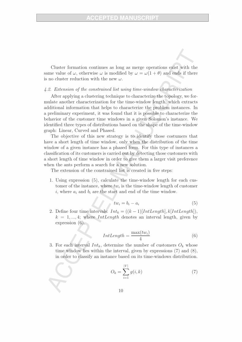
After applying a clustering technique to characterize the topology, we for-mulate another characterization for the time-window length, which extractsadditional information that helps to characterize the problem instances. Ina preliminary experiment, it was found that it is possible to characterize thebehavior of the customer time windows in a given Solomon’s instance. Weidentified three types of distributions based on the shape of the time-windowgraph: Linear, Curved and Phased.
The objective of this new strategy is to identify those costumers thathave a short length of time window, only when the distribution of the timewindow of a given instance has a phased form. For this type of instances aclassification of its customers is carried out by detecting those customers witha short length of time window in order to give them a larger visit preferencewhen the ants perform a search for a new solution.
The extension of the constrained list is created in five steps:
1. Using expression (5), calculate the time-window length for each cus-tomer of the instance, where twi is the time-window length of customeri, where ai and bi are the start and end of the time window.
twi = bi − ai (5)
2. Define four time intervals: Intk = ((k − 1)[IntLength], k[IntLength]),k = 1, ..., 4; where IntLength denotes an interval length, given byexpression (6).
IntLength =max(twi)
4(6)
3. For each interval Intk, determine the number of customers Ok whosetime window lies within the interval, given by expressions (7) and (8),in order to classify an instance based on its time-windows distribution.
Ok =
|V |∑
i=1
g(i, k) (7)
10

where
g(i, k) =
1 if twi ∈ Intk0 otherwise
(8)
4. Determine the number of non-empty intervals I using expression (9),then fill the priority table P of size n×n, when I = 2 and some visitingpreferences between customers are satisfied.
I =∑4
k=1 g(k) ; where
g(k) =
1 if Ok > 00 otherwise
(9)
5. Determine the priority of (i, j ) (pij in expression (10) for each pair(i, j) ∈ A, where i is the current customer, j and k are yet unassignedto the path).
pij =
3 if I = 2 ∧ (twi, twj) ∈ IntminSet ∧ wait1ij < λ1,2 if I = 2 ∧ wait1ij ≥ λ1 ∧ wait2ij < λ2 ∧ deik < λ2,0 otherwise
(10)
where minSet = mini∈[0,4]i|Oi ≥ 1, wait2ij = aj − (ai + si + deik + sk)and wait1ij = (aj − ai − si)− deij. Parameters ai and aj are the time-window start for customers i and j, si is the service time of customeri, deij is the Euclidian distance and λ1 and λ2 are waiting thresholds.Priority levels two and three are only for phased instances I= 2). Levelthree is for a pair of customers (i, j), both customers with short time-window length (they belong to the first enabled interval) and with anacceptable waiting time between customers i and j bounded by λ1.Pairs of customers with level two do not have acceptable waiting timebetween them, but they have an intermediate customer to meet thiscondition.
As a result of applying the ECL in the Solomon’s set [17], the distributionspermit identifying three types of time windows:
Type 1: Linear DistributionIn Figure 3-a we show an example of linear distribution, where time-
window lengths are constant for all the customers in the instance. We foundthat there were 12 instances out of the entire set of 56, which have a lineardistribution; this constitutes approximately 21% of the total.
11

0
50
100
150
200
250
300
0 10 20 30 40 50 60 70 80 90 100
LE
NG
TH
( u
nits
)
CUSTOMER ( i )
a) LINEAR DISTRIBUTION (C107)
Time Window
0
50
100
150
200
0 10 20 30 40 50 60 70 80 90 100
LE
NG
TH
( u
nits
)
CUSTOMER ( i )
b) CURVED DISTRIBUTION (C105)
Time Window
Figure 3: Two types of distribution: a) Linear Distribution, b) Curved Distribution
Type 2: Curved DistributionWe defined curved behavior when costumers have uniform differences in
length from each other in a certain instance as can be seen in Figure 3-b. Wefound that 33% of the instances show a curved behavior in their time-windowdistribution.
Type 3: Phased DistributionIn Figures 4 and 5, we present an example for phased distribution for
the time-window length. We found that phased distribution occurs in 26
12

instances out of the total of 56; this constitutes 46% for the total instances.In the graph of phased distribution two groups of costumers are clearly dis-cerned, those who have a small time-window length and those that have largetime-window length. A particular feature in this type of distribution is thepercentage of customers who have long lengths, which can constitute 25%,50% or 75% of all the costumers. The most interesting structure of the in-stances is the phased distribution that constitutes about 50% of the instancesin the Solomon’s benchmark. Since this distribution makes the distinctionbetween two groups of costumers (those with short length and long length),it is convenient to use this information to improve the ACS algorithm.
0
200
400
600
800
1000
1200
1400
0 10 20 30 40 50 60 70 80 90 100
LE
NG
TH
( u
nits
)
CUSTOMER ( i )
PHASED DISTRIBUTION (C104)
Time Window
Figure 4: Another type of distribution: Phased Distribution 25%
13

0
500
1000
1500
2000
2500
3000
3500
4000
0 10 20 30 40 50 60 70 80 90 100
LE
NG
TH
( u
nits
)
CUSTOMER ( i )
PHASED DISTRIBUTION (C203)
Time Window
0
200
400
600
800
1000
1200
1400
0 10 20 30 40 50 60 70 80 90 100
LE
NG
TH
( u
nits
)
CUSTOMER ( i )
PHASED DISTRIBUTION (C102)
Time Window
Figure 5: Another type of distribution: Phased Distribution 50% and 75%
4.3. Selection of candidates for incorporation into routes
Once the membership into a group based on topological distribution (Sub-section 4.1) and priority based on time-window length distribution (Subsec-tion 4.2) of each customer has been defined, the candidate selection is per-formed according to the selection rule used primarily to update the pheromoneand heuristic information:
• Information of artificial pheromone trails τ , which determines themovement preference from one customer to another; this preferenceis modified during the execution of the algorithm depending on thesolutions as they are being obtained.
14

• Heuristic information η, which measures the preference for the path,including information from the constrained list using topological char-acterization and the characterization of the constrained list extensionby using time-window length.
The selection rule shown in expression (11), is controlled by a balanceparameter q0 ∈ [0, 1] and a random value q. When q ≤ q0, it exploitsthe knowledge available, choosing the best option according to the heuristicinformation and the pheromone trails. However, if q > q0, it applies anexploration for new movements from customer i to customers j.
s =
arg max
j∈N(i)τij [ηij ]
β if q ≤ q0
S otherwise(11)
S = f(prob(i, j)) where prob(i, j) =τij [ηij]
β
∑
k∈N(i)
τik[ηik]β
(12)
In expression (11) β is the relative importance of the heuristic informa-tion, N(i) is the set of available neighbor customers and S is a randomfunction that selects customer j according to a probability distribution givenby expression (12).
The value for η is calculated as follows: if the source customer vi and thedestination customer vj belong to different clusters (hl 6= hm) a correctionfactor to the heuristic information is applied (see expression (13)), whichdepends on the size of the set of costumers V and the size of the set ofclusters H ; otherwise, the priority setting established by the time-windowlength is used.
ηij =
ηij
|H||V | if hl 6= hm ∧ vi ∈ hl ∧ vj ∈ hm
ηij pij otherwise(13)
where hl, hm ∈ H (cluster set), vi, vj ∈ V (customers) and pij denotes time-window information.
4.4. Learning Levels
Learning levels (LL) defines two levels of knowledge: global and local.The first level consists of the values of the original pheromone table τ , which
15

only contains the information of the best solution (ψgs) obtained by the antsand it is modified only in the global updating process.
true
false
new generation
Figure 6: Allocation process for learning levels
The second level consists of the copy of the pheromone table Cτ , whichcontains the local values of the pheromone and it is used by the ants as a guidewhen searching for better solutions. During a local update process, each antupdates its copy of the pheromone table Cτij . The global pheromone tabletakes the best local pheromone table. The allocation process for learninglevels is described in Figure 6 [4].
5. Computational Results
The computational experiments were done on a computer with an IntelXeon 5120 with 2 cores at 1.86 GHz with 3.0 GB of RAM. The operatingsystem was Windows XP Service Pack 3 (32bits), with the IDE of MicrosoftVisual C# Express 2010. For the hypothesis test the SPSS software wasused. The ACS algorithm parameter values used were n = 10 for artificialants and α = 1, q0 = 0.65, β = 6 and ρ = 0.1. The stopping conditionwas 1800 seconds for each Solomon’s instance [17]. In the VRPTW context,the most common way to compare the performance of heuristic algorithmsis solving the instances of the Solomon’s benchmark [17].
These problem instances include a central depot and a variety of: cus-tomers, capacity constraints, demand constraints, and time-window distri-butions. The objective for real applications of VRPTW is to minimize thenumber of required vehicles. Therefore, we carried out a series of experiments
16
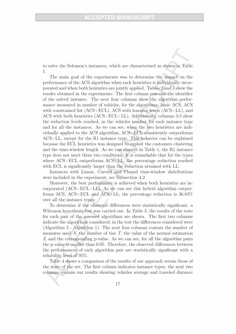
to solve the Solomon’s instances, which are characterized as shown in Table1.
The main goal of the experiments was to determine the impact on theperformance of the ACS algorithm when each heuristics is individually incor-porated and when both heuristics are jointly applied. Tables 2 and 3 show theresults obtained in the experiments. The first column contains the identifierof the solved instance. The next four columns show the algorithm perfor-mance measured in number of vehicles, for the algorithms: basic ACS, ACSwith constrained list (ACS+ECL), ACS with learning levels (ACS+LL), andACS with both heuristics (ACS+ECL+LL). Additionally, columns 3-5 showthe reduction levels reached, in the vehicles number for each instance typeand for all the instances. As we can see, when the two heuristics are indi-vidually applied to the ACS algorithm, ACS+ECL consistently outperformsACS+LL, except for the R1 instance type. This behavior can be explainedbecause the ECL heuristics was designed to exploit the customers clusteringand the time-window length. As we can observe in Table 1, the R1 instancetype does not meet these two conditions. It is remarkable that for the typeswhere ACS+ECL outperforms ACS+LL, the percentage reduction reachedwith ECL is significantly larger than the reduction attained with LL.
Instances with Linear, Curved and Phased time-window distributionswere included in the experiment, see Subsection 4.2.
Moreover, the best performance is achieved when both heuristics are in-corporated (ACS+ECL+LL). As we can see this hybrid algorithm outper-forms ACS, ACS+ECL and ACS+LL; the percentage reduction is 36.83%over all the instance types.
To determine if the observed differences were statistically significant, aWilcoxon hypothesis test was carried out. In Table 3, the results of the testsfor each pair of the assessed algorithms are shown. The first two columnsindicate the algorithms considered; in the test the differences considered were(Algorithm 2 - Algorithm 1). The next four columns contain the number ofmeasures used N, the number of ties T, the value of the normal estimationZ, and the corresponding p-value. As we can see, for all the algorithm pairsthe p-value is smaller than 0.05. Therefore, the observed differences betweenthe performances of each algorithm pair are statistically significant with areliability level of 95%.
Table 4 shows a comparison of the results of our approach versus those ofthe state of the art. The first column indicates instance types, the next twocolumns contain our results showing vehicles average and traveled distance
17
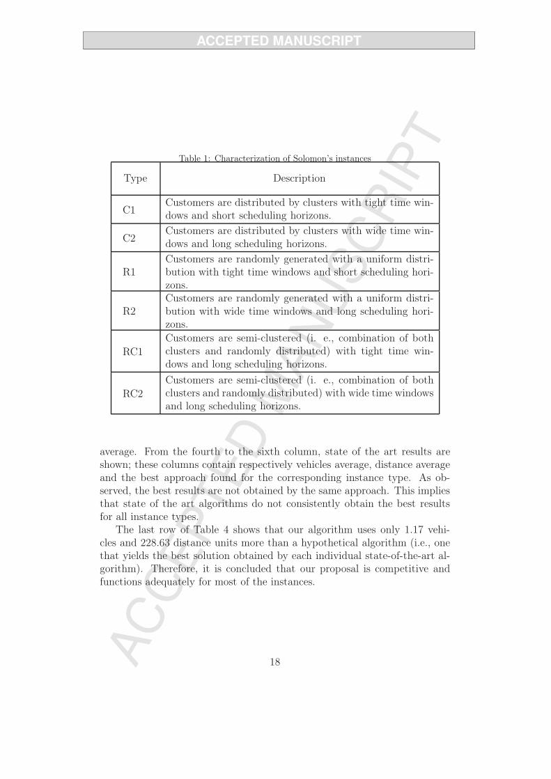
Table 1: Characterization of Solomon’s instances
Type Description
C1Customers are distributed by clusters with tight time win-dows and short scheduling horizons.
C2Customers are distributed by clusters with wide time win-dows and long scheduling horizons.
R1Customers are randomly generated with a uniform distri-bution with tight time windows and short scheduling hori-zons.
R2Customers are randomly generated with a uniform distri-bution with wide time windows and long scheduling hori-zons.
RC1
Customers are semi-clustered (i. e., combination of bothclusters and randomly distributed) with tight time win-dows and long scheduling horizons.
RC2
Customers are semi-clustered (i. e., combination of bothclusters and randomly distributed) with wide time windowsand long scheduling horizons.
average. From the fourth to the sixth column, state of the art results areshown; these columns contain respectively vehicles average, distance averageand the best approach found for the corresponding instance type. As ob-served, the best results are not obtained by the same approach. This impliesthat state of the art algorithms do not consistently obtain the best resultsfor all instance types.
The last row of Table 4 shows that our algorithm uses only 1.17 vehi-cles and 228.63 distance units more than a hypothetical algorithm (i.e., onethat yields the best solution obtained by each individual state-of-the-art al-gorithm). Therefore, it is concluded that our proposal is competitive andfunctions adequately for most of the instances.
18
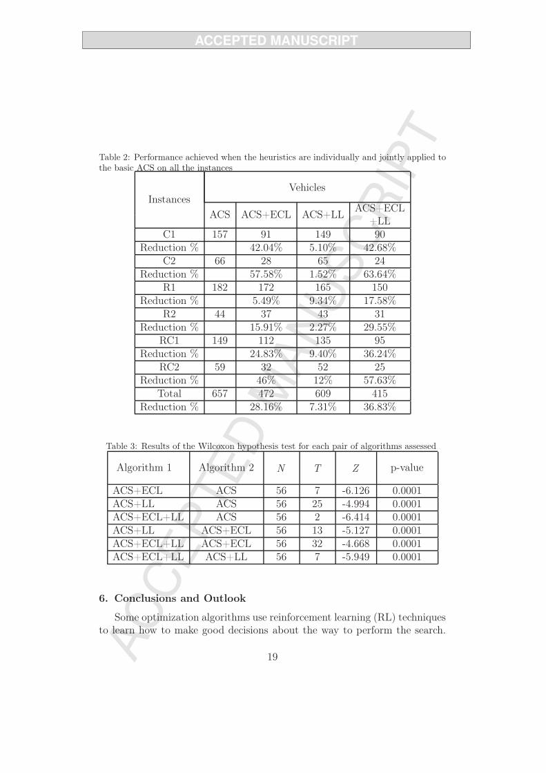
Table 2: Performance achieved when the heuristics are individually and jointly applied tothe basic ACS on all the instances
InstancesVehicles
ACS ACS+ECL ACS+LLACS+ECL
+LLC1 157 91 149 90
Reduction % 42.04% 5.10% 42.68%C2 66 28 65 24
Reduction % 57.58% 1.52% 63.64%R1 182 172 165 150
Reduction % 5.49% 9.34% 17.58%R2 44 37 43 31
Reduction % 15.91% 2.27% 29.55%RC1 149 112 135 95
Reduction % 24.83% 9.40% 36.24%RC2 59 32 52 25
Reduction % 46% 12% 57.63%Total 657 472 609 415
Reduction % 28.16% 7.31% 36.83%
Table 3: Results of the Wilcoxon hypothesis test for each pair of algorithms assessed
Algorithm 1 Algorithm 2 N T Z p-value
ACS+ECL ACS 56 7 -6.126 0.0001ACS+LL ACS 56 25 -4.994 0.0001ACS+ECL+LL ACS 56 2 -6.414 0.0001ACS+LL ACS+ECL 56 13 -5.127 0.0001ACS+ECL+LL ACS+ECL 56 32 -4.668 0.0001ACS+ECL+LL ACS+LL 56 7 -5.949 0.0001
6. Conclusions and Outlook
Some optimization algorithms use reinforcement learning (RL) techniquesto learn how to make good decisions about the way to perform the search.
19

Table 4: Comparative results of state-of-the-art approaches versus our proposed approach
Instance typeOur approach State of the art
Vehicles Distance Vehicles Distance Work
C1 10 829.59 10 828.38 [17]C2 3 593.88 3 589.86 [17]R1 12.5 1234.88 11.92 1210.3 [10]R2 2.82 1057.42 2.73 954.27 [9]
RC1 11.88 1441.89 11.5 1384.2 [9]RC2 3.38 1146.5 325 1108.52 [17]
TOTAL 43.56 6304.16 42.4 6075.53 –
The RL search methods fall into two main categories [22, 21, 20]: model-based and model-free.
Model-based search (MBS) builds a probabilistic model of the searchspace and then uses this model to build new solutions to the problem underconsideration. The reinforcement feedback from the previously seen solutionsis used to improve the model, which is subsequently used to generate newfeasible solutions, in such a way that the search will concentrate on theregions containing high quality solutions. The reuse of information stored inits internal model can facilitate decisions and learning in searching of actionsthat give the largest rewards. However, as the numbers of available actions,possible outcomes, and steps to reach the goal increase, the search requiresa large amount of execution time and working memory.
Model-free search (MFS) is an approach that learns directly from expe-rience and searches the solution space without relying on a predictive modelof performance to guide the search. An action can be selected greedilyor stochastically by comparing the action values of the candidate actions.Model-free search is computationally fast for making estimations. However,it is very slow in terms of its convergence to the optimal solution.
Ant colony optimization (ACO) belongs to the class of model-based searchalgorithms [21]. In general, the ACO approach attempts to solve an opti-mization problem by repeating the following two steps: candidate solutionsare constructed using a pheromone model, which provides positive feedback;
20
and the candidate solutions are used to modify the pheromone values. ACOalgorithms can easily converge to suboptimal solutions if the positive feed-back is not carefully controlled [19]. The Ant Colony System (ACS) is oneof the most successful ACO variants in practice.
In this work the solution of the Vehicle Routing Problem with Time Win-dows (VRPTW) using ACS is approached. A state-of-the-art implementationof ACS uses a constrained list to incorporate geographic information of thecustomers. We propose an extended constrained list (ECL) to include infor-mation of time-window lengths, for identifying those customers with a smalllength of time window in order to give them a larger visit priority when theants search for a new solution.
ECL is a model-free method proposed to control the pheromone feedbackby increasing the selective pressure toward a solution with desired character-istics. This selective pressure reduces the execution time required by ACSand increases its accuracy. In this sense, the model-free ECL provides com-plementary estimates for guiding the preferences of the model-based ACS.To the best of our knowledge, the integration of model-based and model-freefor VRPTW has not been reported previously. We believe that a wide vari-ety of routing approaches may benefit from the integration of these types ofmodels.
A series of experiments were conducted to determine the impact on theperformance of the ACS algorithm when the ECL heuristics is incorporatedalone, and when ECL is complemented by the Learning Levels (LL) heuris-tics. The computational results show that when the two heuristics are in-dividually applied on the ACS algorithm, ECL consistently outperforms LLexcept for the R1 instance type. Also we can see that the hybrid algorithmACS+ECL+LL outperforms algorithms ACS, ACS+ECL and ACS+LL overall the instance types and all the instances. For all the instances the percent-age reduction attained is 36.83%. The experimental results also reveal thatour proposal is competitive with state-of-the-art algorithms.
The hybridization ACS+ECL+LL has only been analyzed with the antcolony system proposed by the authors for VRPTW. Future work is neededto determine the generality of our results. First, it would be interesting toincorporate ECL+LL in other state-of-the-art ACO algorithms. Second, webelieve it would be of great importance the study of the performance of eachheuristics applied to other algorithms and problems. Since ECL is associatedwith forming groups in a graph, ECL could complement the selection of thenext action in search algorithms for graph problems. Besides, we believe
21

that if we change our grouping method by another general-purpose method,ECL could also be applied to other problems to complement the selectionof actions. Regarding the second heuristics, since LL is associated with theuse in two phases of a probabilistic model, this simple heuristics could beexploited by model-based search algorithms.
References
[1] P. Toth and D. Vigo, The vehicle routing problem, SIAM Monographson Discrete Mathematics and Applications, Philadelphia, USA, 2002.
[2] L. Cruz, J. Delgado, J. González, J. Torres, H. Fraire and B. Arrañaga,An ant colony system to solve routing problems applied to the deliveryof bottled products, Lecture Notes in Computer Science 4994 (2008)329-338.
[3] L. Cruz, J. González, J. Delgado, B. Arrañaga and H. Fraire, A newapproach to improve the ant colony system performance: learning levels,Lecture Notes in Computer Science 5572 (2009) 670-677.
[4] J. González, J. Delgado, L. Cruz, H. Fraire and A. Ramirez, Com-parative analysis of hybrid techniques for an ant colony system algo-rithm applied to solve a real-world transportation problem, P. Melin, J.Kacprzyk, W. Pedrycz (Eds.), Soft Computing for Recognition Basedon Biometrics Studies in Computational Intelligence, 2010, pp. 365-385.
[5] E. Mariano and F. Morales, DQL: A new updating strategy for reinforce-ment learning based on q-learning, Lecture Notes in Computer Science2167 (2001), 324-335.
[6] C. Gómez, L. Cruz, M. Morales, J. González, O. Castillo, G. Riveraand P. Hernández, Variants of VRP to optimize logistics managementproblems, C. Ortiz Zezzatti, C. Chira, A. Hernandez, M. Basurto (Eds.),Logistics Management and Optimization through Hybrid Artificial In-telligence Systems, 2012, pp. 207-237.
[7] D. Pisinger and S. Ropke, A general heuristic for vehicle routing prob-lems, Computers and Operations Research 34 (2007), 2403-2435.
22

[8] P. Shaw, Using constraint programming and local search methods tosolve vehicle routing problems, M. Maher, J. Puget (Eds.), Lecture Notesin Computer Science, Germany, 1998, pp. 417-431.
[9] D. Mester, O. Bräysy and W. Dullaert, A multi-parametric evolutionstrategies algorithm for vehicle routing problems, Expert Systems withApplications 32 (2007), 508-517.
[10] E. Prescott-Gagnon, G. Desaulniers, and L.M. Rousseau, A branch-and-price based large neighborhood search algorithm for the vehicle routingproblem with time windows, Networks 54 (2009), 190-204.
[11] T. Hoshino, T. Kimura and T. Ikeguchi, Two simple local searches con-trolled by chaotic dynamics for the vehicle routing problems with timewindows, In Abstract Proceedings of The Seventh Metaheuristics Inter-national Conference MIC 2007, Canada, 2007, pp.25-29.
[12] O. Bräysy, A reactive varaible neighborhood search for the vehicle rout-ing problem with time windows, INFORMS Journal on Computing 15(2003), 347-368.
[13] S. Thangiah, A site dependent vehicle routing problem with complexroad constraints, Proceedings of International Conference on Meta-heuristics for Optimization (2003), 1-17.
[14] G. Dantzig and J. Ramser, The truck dispatching problem, ManagementScience 6 (1959), 80-91.
[15] B. Kallehauge, Formulations and exact algorithms for the vehicle routingproblem with time windows, Computers & Operations Research 35(7)(2008), 2307-2330.
[16] M. Dorigo and C. Blum, Ant colony optimization theory: a survey,Theoretical Computer Science 344 (2005), 243-278.
[17] M. Solomon, Algorithms for the vehicle routing and scheduling problemswith time window constraints, Operations Research 35 (1987), 254-265.
[18] N. Park, H. Okano and H. Imai, A path-exchange-type local searchalgorithm for vehicle routing and its efficient search strategy, Journal ofthe Operations Research Society of Japan 43 (2000), 197-208.
23
[19] J. Dowling, E. Curran, R. Cunningham, V. Cahill, Using feedback in col-laborative reinforcement learning to adaptively optimize MANET rout-ing, IEEE Transactions on Systems, Man and Cybernetics - Part A:Systems and Humans 35 (2005) 360-372.
[20] A. Haith, J. Krakauer, Model-based and model-free mechanisms of hu-man motor learning, M. Richardson, M. Riley, K. Shockley (Eds.),Progress in Motor Control, Advances in Experimental Medicine andBiology 782 (2013) 1-21.
[21] H. Ping, A stochastic approximation interpretation for model-based op-timization algorithms, Ph.D. thesis, Stony Brook University, USA, 2012.
[22] M. Zlochin, M. Birattari, N. Meuleau, M. Dorigo. Model-based searchfor combinatorial optimization: a critical survey, Annals of OperationsResearch 131 (2004) 373-395.
24

Computación y Sistemas Vol. 16 No.3, 2012 pp 349-360 ISSN 1405-5546
Heurísticas de agrupación híbridas eficientes para el problema de empacado de objetos en contenedores
Laura Cruz-Reyes1, Marcela Quiroz C.1, Adriana C. F. Alvim2, Héctor J. Fraire Huacuja1, Claudia Gómez S.1 y José Torres-Jiménez3
1 Instituto Tecnológico de Ciudad Madero, México
2 Universidad Federal do Estado do Rio de Janeiro, Brasil
3 Centro de Investigación y de Estudios Avanzados del Instituto Politécnico Nacional, México
[email protected], [email protected], [email protected], [email protected], [email protected], [email protected]
Resumen. En este artículo se aborda un problema clásico muy conocido por su aplicabilidad y complejidad: el empacado de objetos en contenedores (Bin Packing Problem, BPP). Para la solución de BPP se propone un algoritmo genético híbrido de agrupación denominado HGGA-BP. El algoritmo propuesto está inspirado en el esquema de representación de grupos de Falkenauer, el cual aplica operadores evolutivos a nivel de contenedores. HGGA-BP incluye heurísticas eficientes para generar la población inicial y realizar mutación y cruzamiento de grupos; así como estrategias híbridas para el acomodo de objetos que quedaron libres al aplicar los operadores grupales. La efectividad del algoritmo es comparable con la de los mejores del estado del arte, superando los resultados publicados para el conjunto de instancias hard28, el cual ha mostrado el mayor grado de dificultad para los algoritmos de solución de BPP.
Palabras clave. Metodologías computacionales, inteligencia artificial, solución de problemas, problema de empacado de objeto en contenedores, algoritmo genético hibrido.
Efficient Hybrid Grouping Heuristics for the Bin Packing Problem
Abstract. This article addresses a classical problem known for its applicability and complexity: the Bin Packing Problem (BPP). A hybrid grouping genetic algorithm called HGGA-BP is proposed to solve BPP. The proposed algorithm is inspired by the Falkenauer grouping encoding scheme, which applies evolutionary operators at the bin level. HGGA-BP includes efficient
heuristics to generate the initial population and performs mutation and crossover for groups as well as hybrid strategies for the arrangement of objects that were released by the group operators. The effectiveness of the algorithm is comparable with the best state-of-the-art algorithms, outperforming the published results for the class of instances hard28, which has shown the highest difficulty for algorithms that solve BPP.
Keywords. Computer methodologies, artificial intelligence, problem solving, bin packing problem, hybrid genetic algorithm.
1 Introducción
El problema de empacado de objetos en contenedores en una dimensión (one-dimensional Bin Packing Problem BPP), consiste en almacenar un conjunto de objetos de diferentes tamaños N = 1,…,n, o pesos, en el menor número de contenedores de tamaño fijo sin violar la capacidad de ningún contenedor.
BPP es un problema de optimización combinatoria NP-duro, considerado intratable debido a que demanda una gran cantidad de recursos para su solución [2,16]. La importancia de BPP radica en que tiene un extenso número de aplicaciones industriales y logísticas, y gran cantidad de problemas prácticos pueden ser modelados como problemas de empacado [8, 9, 10].

350 Laura Cruz-Reyes, Marcela Quiroz C., Adriana C. F. Alvim, Héctor J. Fraire Huacuja…
Computación y Sistemas Vol. 16 No. 3, 2012 pp. 349-360 ISSN 1405-5546
A lo largo de los últimos veinte años, en la búsqueda de buenas y mejores soluciones para BPP se han diseñado una gran variedad de algoritmos. Los resultados más destacados han sido obtenidos mediante el uso de algoritmos híbridos y metaheurísticos.
Martello y Toth [24] proponen un procedimiento de ramificación y poda (MTP) que incluye un criterio de dominación [23] para reducir el espacio de búsqueda. El criterio de dominación establece que: si es posible intercambiar un conjunto de objetos de un contenedor por un solo objeto del mismo peso que el conjunto, la solución puede ser mejorada debido a que será más fácil distribuir el conjunto de objetos pequeños en el resto de los contenedores, a encontrar un lugar para el objeto grande, debido a que su dominio es mayor. E. Falkenauer [13] propone un algoritmo genético híbrido de agrupación (HGGA) que utiliza: un esquema de representación de la solución por grupos de objetos y un método de optimización local inspirado en el criterio de dominación de Martello y Toth.
Scholl et al. [28] desarrollan un procedimiento híbrido (BISON) que combina una búsqueda tabú con un método de ramificación y poda, usando una estrategia dual que consiste en minimizar el llenado de los contenedores dado un número fijo de éstos. BISON incluye un nuevo esquema de ramificación basado en límites inferiores del valor de la solución óptima. Coffman et al. [7] presentan un estudio exhaustivo de las principales heurísticas deterministas para Bin Packing, incluyendo los análisis del peor caso de los algoritmos FFD y BFD [23]. Schwerin y Wäscher [29] proponen un nuevo límite inferior para BPP basado en problemas de corte y lo integran al método MTP de Martello y Toth [24], obteniendo resultados de calidad con su nuevo algoritmo (MTPCS). Fleszar y Hindi [14] introducen un nuevo algoritmo (Pertubation-MBS´) que incorpora una versión modificada de la heurística MBS de Gupta y Ho [18], una búsqueda de vecindad variable y límites inferiores, obteniendo buenos resultados. Levine y Ducatelle [20] desarrollan un método híbrido (HACO-BP) que implementa la metaheurística de optimización basada en colonia de hormigas; este algoritmo incluye una estrategia de búsqueda
local y se apoya en el criterio de dominación de Martello y Toth [23]. Bhatia y Basu [5] presentan un algoritmo genético de agrupación multi-cromosómico (MGGA) y una nueva heurística de empacado (better-fit).
Alvim et al. [1] proponen una heurística de mejora híbrida (HI_BP) en la que retoman la estrategia dual de Scholl et al. [28], así como las técnicas de reducción de Martello y Toth [23], obteniendo los mejores resultados del estado del arte, hasta ese momento.
Singh y Gupta [31] desarrollan un enfoque evolutivo híbrido (C_BP) que combina un algoritmo genético de agrupación con una versión mejorada de la heurística Perturbation-MBS’ de Fleszar y Hindi [14]. El desempeño obtenido es comparable con la estrategia HI_BP de Alvim et al. [1], sin embargo, el algoritmo C_BP es menos robusto.
A. Stawowy [32] propone una nueva estrategia evolutiva no especializada (ES) que incluye mutaciones inteligentes, una técnica de reducción del tamaño del problema y un esquema de representación basado en permutaciones con separadores de grupos. Los resultados obtenidos por el metaheurístico no hibridizado son comparables con los de algoritmos mucho más complicados. Rohlfshagen y Bullinaria [26] desarrollan un algoritmo genético inspirado en el proceso de formación de proteínas (ESGA) que obtiene resultados prometedores al ser comparado con otras estrategias.
Loh et al. [22] desarrollan un procedimiento (WA) que hace uso del concepto de recocido de pesos, el algoritmo propuesto es sencillo y fácil de implementar y obtiene un desempeño de alta calidad superando al mejor algoritmo del estado del arte, HI_BP [1].
Gómez-Meneses y Randall [17] presentan un procedimiento evolutivo híbrido de optimización extrema (HEO) que incorpora una búsqueda local para mejorar el empacado de los contenedores. R. Lewis [21] propone un algoritmo de escalado de colina (HC) que utiliza un esquema sencillo de mejora basado en el criterio de dominación y obtiene buenas soluciones superando, en algunos casos, el desempeño de algoritmos complejos.
El último trabajo en esta área fue presentado por Fleszar y Charalambous [15], los autores
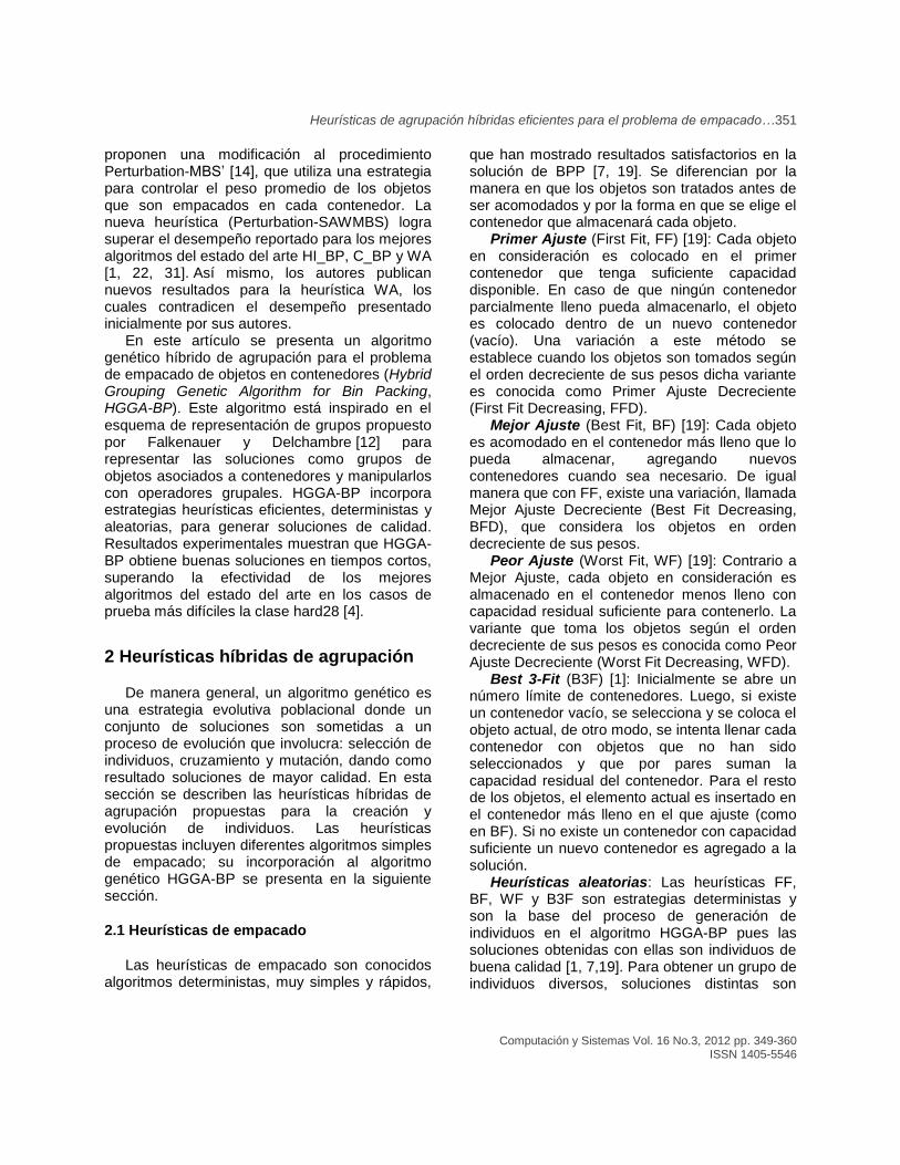
Heurísticas de agrupación híbridas eficientes para el problema de empacado…351
Computación y Sistemas Vol. 16 No.3, 2012 pp. 349-360 ISSN 1405-5546
proponen una modificación al procedimiento Perturbation-MBS’ [14], que utiliza una estrategia para controlar el peso promedio de los objetos que son empacados en cada contenedor. La nueva heurística (Perturbation-SAWMBS) logra superar el desempeño reportado para los mejores algoritmos del estado del arte HI_BP, C_BP y WA [1, 22, 31]. Así mismo, los autores publican nuevos resultados para la heurística WA, los cuales contradicen el desempeño presentado inicialmente por sus autores.
En este artículo se presenta un algoritmo genético híbrido de agrupación para el problema de empacado de objetos en contenedores (Hybrid Grouping Genetic Algorithm for Bin Packing, HGGA-BP). Este algoritmo está inspirado en el esquema de representación de grupos propuesto por Falkenauer y Delchambre [12] para representar las soluciones como grupos de objetos asociados a contenedores y manipularlos con operadores grupales. HGGA-BP incorpora estrategias heurísticas eficientes, deterministas y aleatorias, para generar soluciones de calidad. Resultados experimentales muestran que HGGA-BP obtiene buenas soluciones en tiempos cortos, superando la efectividad de los mejores algoritmos del estado del arte en los casos de prueba más difíciles la clase hard28 [4].
2 Heurísticas híbridas de agrupación
De manera general, un algoritmo genético es una estrategia evolutiva poblacional donde un conjunto de soluciones son sometidas a un proceso de evolución que involucra: selección de individuos, cruzamiento y mutación, dando como resultado soluciones de mayor calidad. En esta sección se describen las heurísticas híbridas de agrupación propuestas para la creación y evolución de individuos. Las heurísticas propuestas incluyen diferentes algoritmos simples de empacado; su incorporación al algoritmo genético HGGA-BP se presenta en la siguiente sección.
2.1 Heurísticas de empacado
Las heurísticas de empacado son conocidos algoritmos deterministas, muy simples y rápidos,
que han mostrado resultados satisfactorios en la solución de BPP [7, 19]. Se diferencian por la manera en que los objetos son tratados antes de ser acomodados y por la forma en que se elige el contenedor que almacenará cada objeto.
Primer Ajuste (First Fit, FF) [19]: Cada objeto en consideración es colocado en el primer contenedor que tenga suficiente capacidad disponible. En caso de que ningún contenedor parcialmente lleno pueda almacenarlo, el objeto es colocado dentro de un nuevo contenedor (vacío). Una variación a este método se establece cuando los objetos son tomados según el orden decreciente de sus pesos dicha variante es conocida como Primer Ajuste Decreciente (First Fit Decreasing, FFD).
Mejor Ajuste (Best Fit, BF) [19]: Cada objeto es acomodado en el contenedor más lleno que lo pueda almacenar, agregando nuevos contenedores cuando sea necesario. De igual manera que con FF, existe una variación, llamada Mejor Ajuste Decreciente (Best Fit Decreasing, BFD), que considera los objetos en orden decreciente de sus pesos.
Peor Ajuste (Worst Fit, WF) [19]: Contrario a Mejor Ajuste, cada objeto en consideración es almacenado en el contenedor menos lleno con capacidad residual suficiente para contenerlo. La variante que toma los objetos según el orden decreciente de sus pesos es conocida como Peor Ajuste Decreciente (Worst Fit Decreasing, WFD).
Best 3-Fit (B3F) [1]: Inicialmente se abre un número límite de contenedores. Luego, si existe un contenedor vacío, se selecciona y se coloca el objeto actual, de otro modo, se intenta llenar cada contenedor con objetos que no han sido seleccionados y que por pares suman la capacidad residual del contenedor. Para el resto de los objetos, el elemento actual es insertado en el contenedor más lleno en el que ajuste (como en BF). Si no existe un contenedor con capacidad suficiente un nuevo contenedor es agregado a la solución.
Heurísticas aleatorias: Las heurísticas FF, BF, WF y B3F son estrategias deterministas y son la base del proceso de generación de individuos en el algoritmo HGGA-BP pues las soluciones obtenidas con ellas son individuos de buena calidad [1, 7,19]. Para obtener un grupo de individuos diversos, soluciones distintas son

352 Laura Cruz-Reyes, Marcela Quiroz C., Adriana C. F. Alvim, Héctor J. Fraire Huacuja…
Computación y Sistemas Vol. 16 No. 3, 2012 pp. 349-360 ISSN 1405-5546
obtenidas al manejar órdenes aleatorios del conjunto de objetos a acomodar. Las versiones aleatorias de las heurísticas de empacado han sido denominadas: FF_Aleatorio, BF_Aleatorio, WF_Aleatorio y B3F_Aleatorio, respectivamente.
2.2 Construcción de individuos
Todas las estrategias de construcción de individuos inician con el cálculo de un límite inferior del número de contenedores LM, que es igual al número de objetos de tamaño mayor que la mitad de la capacidad del contenedor. LM representa el número de objetos “grandes” que no podrían combinarse entre sí. Una vez calculado dicho límite, los LM objetos más pesados son almacenados cada uno en un contenedor y el resto de los objetos son acomodados con alguna de las técnicas para empacado de objetos descritas en la sección anterior.
2.3 Generación de la población
Con el método PI_ D-A la población inicial se forma con dos tipos de individuos: deterministas y aleatorios. La parte determinista se conforma de cuatro individuos creados con FFD, BFD, WFD, y B3FD. La población aleatoria se compone de individuos creados con las estrategias FF_Aleatorio, BF_Aleatorio, WF_Aleatorio y B3F_Aleatorio.
El cálculo de la Aptitud de cada individuo de la población es realizado utilizando la función de costo introducida por Falkenauer y Delchambre, que evalúa el promedio de llenado de los contendores que conforman una solución [12]. Dado que, según esta función, las soluciones que poseen un mayor promedio de llenado son mejores, el objetivo del algoritmo HGGA-BP es maximizar el valor de las aptitudes de los individuos que conforman la población. La Ecuación 1 define el cálculo de la aptitud, donde m es el número de contenedores utilizado en la solución, Si es la suma de los tamaños de los objetos en el contenedor i y c es la capacidad del contenedor.
2
1
/m
i
i
S c
Aptitudm
(1)
2.4 Operadores genéticos para grupos
Un esquema de codificación por agrupación para BPP fue propuesto por Falkenauer y Delchambre [12]. En este tipo de estructura cromosómica los genes del individuo están representados por contenedores y no por objetos. Para manipular grupos de objetos en el algoritmo HGGA-BP se propone utilizar operadores genéticos especiales y heurísticas de reacomodo de objetos que quedan libres al aplicar dichos operadores.
2.4.1 Heurísticas de reacomodo de objetos
En el proceso de solución, los operadores genéticos generan y modifican individuos, producto de este proceso algunos contenedores son vaciados y existen objetos libres que necesitan ser reinsertados en la solución. En este trabajo se proponen dos nuevos procedimientos de reacomodo.
Reacomodo_Voraz: Este procedimiento recorre cada contenedor intentando intercambiar uno de sus objetos por un objeto libre de mayor tamaño, sin violar su capacidad. Después de recorrer todos los contenedores, los objetos libres se reacomodan utilizando la heurística de empacado BFD.
Reacomodo_por_Pares: Esta estrategia consta de dos etapas: Generar una permutación aleatoria del orden de los contenedores y recorrer por pares todos los objetos de cada contenedor intentando intercambiar el par de objetos por una mejor opción. Las alternativas de sustitución son dos: a) Sustituir el par de objetos del contenedor por un objeto libre de peso igual o mayor que no sobrepase la capacidad del contenedor y b) Sustituir el par de objetos del contenedor por un par de objetos diferentes que sumen lo mismo o que llenen más el contenedor. Finalmente, si existen objetos libres, la heurística BF_Aleatorio es aplicada para completar la solución.
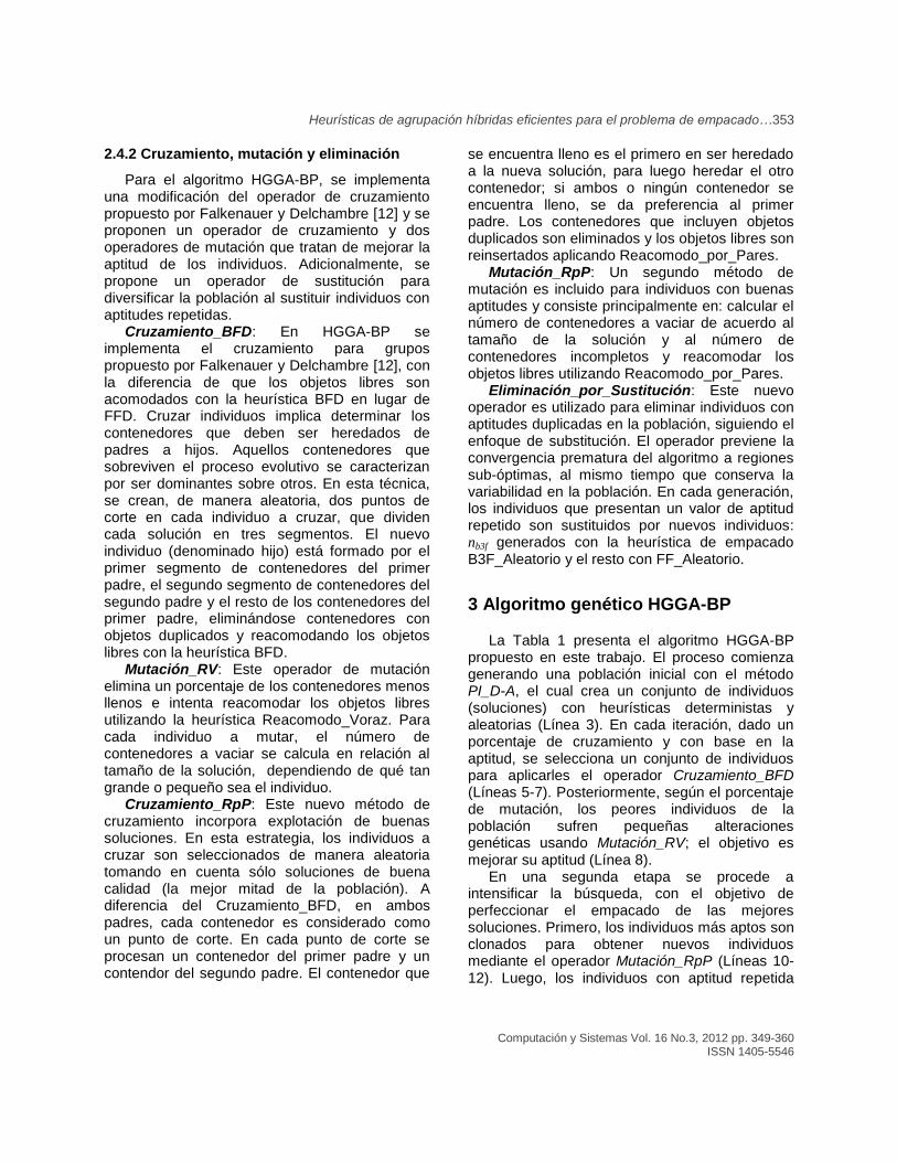
Heurísticas de agrupación híbridas eficientes para el problema de empacado…353
Computación y Sistemas Vol. 16 No.3, 2012 pp. 349-360 ISSN 1405-5546
2.4.2 Cruzamiento, mutación y eliminación
Para el algoritmo HGGA-BP, se implementa una modificación del operador de cruzamiento propuesto por Falkenauer y Delchambre [12] y se proponen un operador de cruzamiento y dos operadores de mutación que tratan de mejorar la aptitud de los individuos. Adicionalmente, se propone un operador de sustitución para diversificar la población al sustituir individuos con aptitudes repetidas.
Cruzamiento_BFD: En HGGA-BP se implementa el cruzamiento para grupos propuesto por Falkenauer y Delchambre [12], con la diferencia de que los objetos libres son acomodados con la heurística BFD en lugar de FFD. Cruzar individuos implica determinar los contenedores que deben ser heredados de padres a hijos. Aquellos contenedores que sobreviven el proceso evolutivo se caracterizan por ser dominantes sobre otros. En esta técnica, se crean, de manera aleatoria, dos puntos de corte en cada individuo a cruzar, que dividen cada solución en tres segmentos. El nuevo individuo (denominado hijo) está formado por el primer segmento de contenedores del primer padre, el segundo segmento de contenedores del segundo padre y el resto de los contenedores del primer padre, eliminándose contenedores con objetos duplicados y reacomodando los objetos libres con la heurística BFD.
Mutación_RV: Este operador de mutación elimina un porcentaje de los contenedores menos llenos e intenta reacomodar los objetos libres utilizando la heurística Reacomodo_Voraz. Para cada individuo a mutar, el número de contenedores a vaciar se calcula en relación al tamaño de la solución, dependiendo de qué tan grande o pequeño sea el individuo.
Cruzamiento_RpP: Este nuevo método de cruzamiento incorpora explotación de buenas soluciones. En esta estrategia, los individuos a cruzar son seleccionados de manera aleatoria tomando en cuenta sólo soluciones de buena calidad (la mejor mitad de la población). A diferencia del Cruzamiento_BFD, en ambos padres, cada contenedor es considerado como un punto de corte. En cada punto de corte se procesan un contenedor del primer padre y un contendor del segundo padre. El contenedor que
se encuentra lleno es el primero en ser heredado a la nueva solución, para luego heredar el otro contenedor; si ambos o ningún contenedor se encuentra lleno, se da preferencia al primer padre. Los contenedores que incluyen objetos duplicados son eliminados y los objetos libres son reinsertados aplicando Reacomodo_por_Pares.
Mutación_RpP: Un segundo método de mutación es incluido para individuos con buenas aptitudes y consiste principalmente en: calcular el número de contenedores a vaciar de acuerdo al tamaño de la solución y al número de contenedores incompletos y reacomodar los objetos libres utilizando Reacomodo_por_Pares.
Eliminación_por_Sustitución: Este nuevo operador es utilizado para eliminar individuos con aptitudes duplicadas en la población, siguiendo el enfoque de substitución. El operador previene la convergencia prematura del algoritmo a regiones sub-óptimas, al mismo tiempo que conserva la variabilidad en la población. En cada generación, los individuos que presentan un valor de aptitud repetido son sustituidos por nuevos individuos: nb3f generados con la heurística de empacado B3F_Aleatorio y el resto con FF_Aleatorio.
3 Algoritmo genético HGGA-BP
La Tabla 1 presenta el algoritmo HGGA-BP propuesto en este trabajo. El proceso comienza generando una población inicial con el método PI_D-A, el cual crea un conjunto de individuos (soluciones) con heurísticas deterministas y aleatorias (Línea 3). En cada iteración, dado un porcentaje de cruzamiento y con base en la aptitud, se selecciona un conjunto de individuos para aplicarles el operador Cruzamiento_BFD (Líneas 5-7). Posteriormente, según el porcentaje de mutación, los peores individuos de la población sufren pequeñas alteraciones genéticas usando Mutación_RV; el objetivo es mejorar su aptitud (Línea 8).
En una segunda etapa se procede a intensificar la búsqueda, con el objetivo de perfeccionar el empacado de las mejores soluciones. Primero, los individuos más aptos son clonados para obtener nuevos individuos mediante el operador Mutación_RpP (Líneas 10-12). Luego, los individuos con aptitud repetida
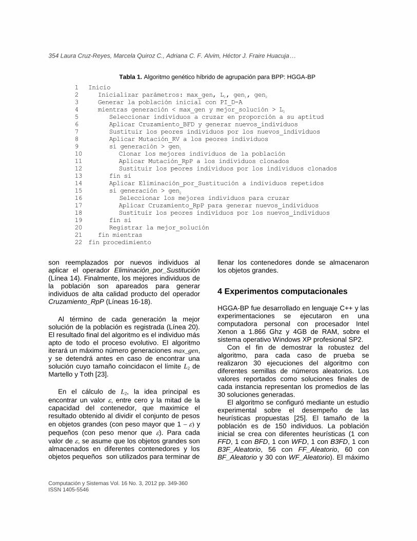
354 Laura Cruz-Reyes, Marcela Quiroz C., Adriana C. F. Alvim, Héctor J. Fraire Huacuja…
Computación y Sistemas Vol. 16 No. 3, 2012 pp. 349-360 ISSN 1405-5546
son reemplazados por nuevos individuos al aplicar el operador Eliminación_por_Sustitución (Línea 14). Finalmente, los mejores individuos de la población son apareados para generar individuos de alta calidad producto del operador Cruzamiento_RpP (Líneas 16-18).
Al término de cada generación la mejor solución de la población es registrada (Línea 20). El resultado final del algoritmo es el individuo más apto de todo el proceso evolutivo. El algoritmo iterará un máximo número generaciones max_gen, y se detendrá antes en caso de encontrar una solución cuyo tamaño coincidacon el límite L2 de Martello y Toth [23].
En el cálculo de L2, la idea principal es encontrar un valor , entre cero y la mitad de la capacidad del contenedor, que maximice el resultado obtenido al dividir el conjunto de pesos en objetos grandes (con peso mayor que 1 y pequeños (con peso menor que ). Para cada valor de , se asume que los objetos grandes son almacenados en diferentes contenedores y los objetos pequeños son utilizados para terminar de
llenar los contenedores donde se almacenaron los objetos grandes.
4 Experimentos computacionales
HGGA-BP fue desarrollado en lenguaje C++ y las experimentaciones se ejecutaron en una computadora personal con procesador Intel Xenon a 1.866 Ghz y 4GB de RAM, sobre el sistema operativo Windows XP profesional SP2.
Con el fin de demostrar la robustez del algoritmo, para cada caso de prueba se realizaron 30 ejecuciones del algoritmo con diferentes semillas de números aleatorios. Los valores reportados como soluciones finales de cada instancia representan los promedios de las 30 soluciones generadas.
El algoritmo se configuró mediante un estudio experimental sobre el desempeño de las heurísticas propuestas [25]. El tamaño de la población es de 150 individuos. La población inicial se crea con diferentes heurísticas (1 con FFD, 1 con BFD, 1 con WFD, 1 con B3FD, 1 con B3F_Aleatorio, 56 con FF_Aleatorio, 60 con BF_Aleatorio y 30 con WF_Aleatorio). El máximo
Tabla 1. Algoritmo genético híbrido de agrupación para BPP: HGGA-BP
1
2
3
4
5
6
7
8
9
10
11
12
13
14
15
16
17
18
19
20
21
22
Inicio
Inicializar parámetros: max_gen, L2, gen
1, gen
2
Generar la población inicial con PI_D-A
mientras generación < max_gen y mejor_solución > L2
Seleccionar individuos a cruzar en proporción a su aptitud
Aplicar Cruzamiento_BFD y generar nuevos_individuos
Sustituir los peores individuos por los nuevos_individuos
Aplicar Mutación_RV a los peores individuos
si generación > gen1
Clonar los mejores individuos de la población
Aplicar Mutación_RpP a los individuos clonados
Sustituir los peores individuos por los individuos clonados
fin si
Aplicar Eliminación_por_Sustitución a individuos repetidos
si generación > gen2
Seleccionar los mejores individuos para cruzar
Aplicar Cruzamiento_RpP para generar nuevos_individuos
Sustituir los peores individuos por los nuevos_individuos
fin si
Registrar la mejor_solución
fin mientras
fin procedimiento

Heurísticas de agrupación híbridas eficientes para el problema de empacado…355
Computación y Sistemas Vol. 16 No.3, 2012 pp. 349-360 ISSN 1405-5546
número de generaciones max_gen es 100. En cada generación se aplican los operadores Cruzamiento_BFD y Mutación_RV al 30% de los individuos de la población. En Mutación_RV, el intervalo de contenedores a vaciar es 10-35%. Después de la décima generación (gen1=10), el operador Mutación_RpP es aplicado, en cada generación, para generar 15 nuevos individuos que sustituyen a las 15 peores soluciones y para introducir pequeñas modificaciones en 15 buenos individuos. Cruzamiento_RpP se utiliza para generar 35 nuevos individuos que sustituyen a las 35 peores soluciones y es aplicado después de la generación número 20 (gen2=20). El operador Eliminación_por_Sustitución es aplicado en cada generación para generar nb3f=3 individuos con la heurística de empacado B3F_Aleatorio y el resto con la estrategia FF_Aleatorio.
4.1 Instancias de prueba
El desempeño de los algoritmos para BPP ha sido evaluado con diferentes clases de instancias de referencia consideradas retadoras. Los casos de prueba, elegidos por diferentes investigadores para comparar las cualidades de sus estrategias con las de otros algoritmos del estado del arte, conforman un conjunto de 1615 casos estándar reconocidos por la comunidad científica. Las 1615 instancias de prueba se encuentran en sitios de Internet reconocidos [3, 6, 11, 27], sus soluciones óptimas son conocidas [1, 4, 27]. Las instancias consideradas se han dividido en cuatro grupos, tomando en cuenta su origen y los sitios de los que fueron obtenidas.
El primer grupo consiste en dos conjuntos de instancias propuestas por E. Falkenauer [13].
Uniform (u) [3]: Conjunto de 80 instancias identificadas con la letra u debido a que su principal característica es que los pesos de los objetos están uniformemente distribuidos entre 20 y 100. La capacidad del contenedor c es de 150 y existen cuatro clases de casos cada uno con n = 120, 250, 500 y 1000 objetos. Cada clase posee 20 instancias identificadas respectivamente por u_120, u_250, u_500 y u_1000. El valor de la solución óptima para cada una de estas instancias es conocido [1].
Triplets (t) [3]: Conjunto de 80 instancias difíciles, identificadas con la letra t. Su nombre se
debe a que las instancias fueron construidas con una solución óptima conocida de n/3 contenedores, de tal forma que cada contenedor de la solución óptima debe almacenar exactamente tres objetos que lo llenan completamente. El tamaño de las instancias es de n = 60, 120, 249 y 501, definiéndose así cuatro clases, el tamaño del contenedor c es de 100, mientras que los pesos están distribuidos entre 25 y 50. Cada clase posee 20 instancias identificadas respectivamente por t_60, t_120, t_249 y t_501.
El segundo grupo está formado por tres conjuntos de casos de prueba introducidos por Scholl et al. [28]. En cada conjunto, las diferentes clases de problemas fueron creados variándose el número de objetos n, la capacidad del contenedor c y los posibles pesos de los objetos.
Data Set 1 (set_1) [27]: Construidas de forma similar que algunas instancias propuestas por Martello y Toth [24] que resultaron difíciles. Son un conjunto de 720 instancias denotadas con n-c-w por los datos que manejan: n = 50, 100, 200 y 500, capacidad del contenedor c = 100, 120, 150 y los pesos w generados uniformemente en intervalos de [1,100], [20,100] y [30,100]. La combinación de los diferentes parámetros resulta en 36 clases, cada clase contiene 20 instancias.
Data Set 2 (set_2) [27]: Incluye 480 instancias con pesos generados con una distribución uniforme, denotadas por n-w-b. Cada sigla representa la configuración de un parámetro de entrada: número de objetos n con valores de 50, 100, 200 y 500, la capacidad de los contenedores c es 1000. Con el objetivo de generar instancias cuyo número medio de objetos por contenedor variara entre tres y nueve, se consideraron otros dos parámetros: el peso medio deseado w con valores c/3, c/5, c/7, c/9, y una desviación máxima de dicho peso b = 20%, 50%, 90%. Por ejemplo cuando w = c/5 y b= 50%, los pesos de los objetos fueron generados de manera aleatoria con una distribución uniforme en el intervalo discreto [100, 300]. Al Combinar las características anteriores se cuenta con 48 clases, cada una con 10 instancias.
Data Set 3 (set_3) [27]: Conjunto formado por una única clase con diez instancias consideradas difíciles. Cada instancia posee 200 objetos, capacidad de contenedor 100000 y los pesos
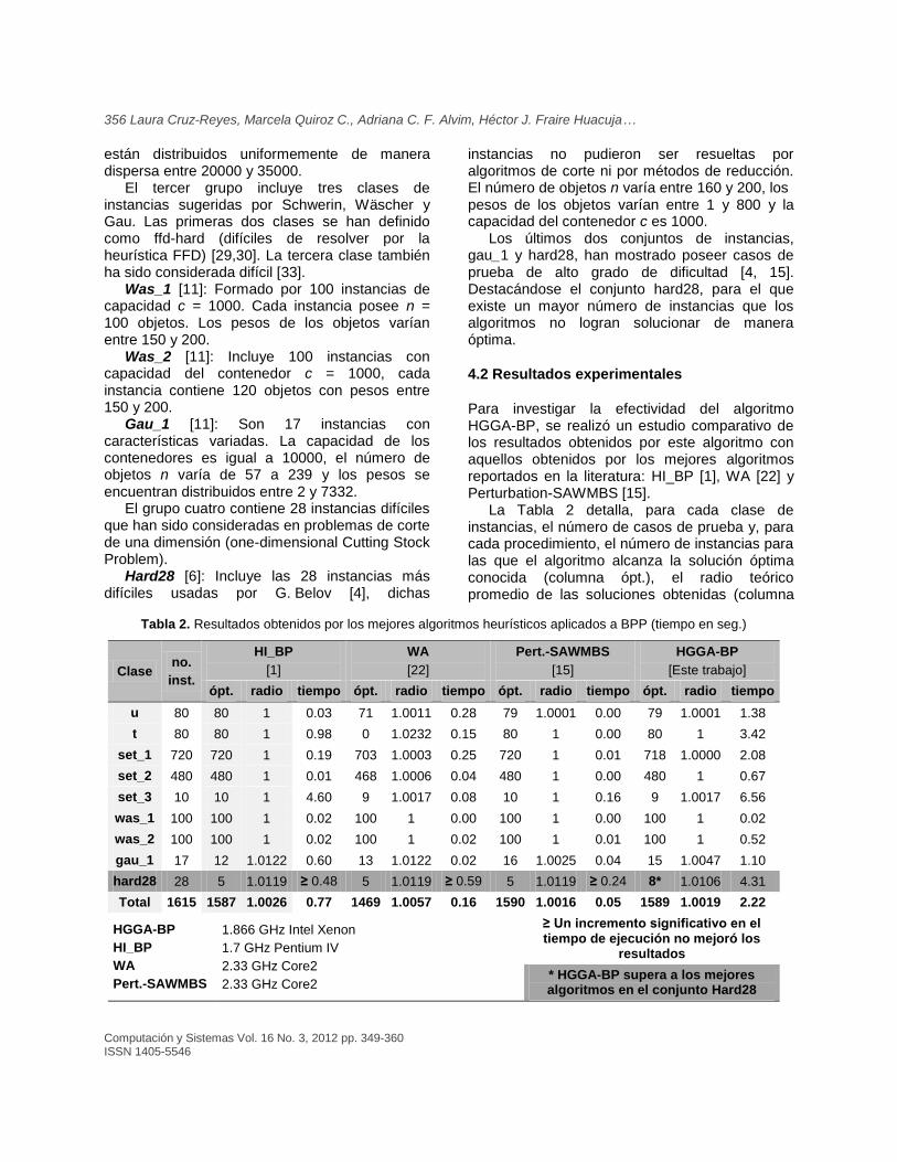
356 Laura Cruz-Reyes, Marcela Quiroz C., Adriana C. F. Alvim, Héctor J. Fraire Huacuja…
Computación y Sistemas Vol. 16 No. 3, 2012 pp. 349-360 ISSN 1405-5546
están distribuidos uniformemente de manera dispersa entre 20000 y 35000.
El tercer grupo incluye tres clases de instancias sugeridas por Schwerin, Wäscher y Gau. Las primeras dos clases se han definido como ffd-hard (difíciles de resolver por la heurística FFD) [29,30]. La tercera clase también ha sido considerada difícil [33].
Was_1 [11]: Formado por 100 instancias de capacidad c = 1000. Cada instancia posee n = 100 objetos. Los pesos de los objetos varían entre 150 y 200.
Was_2 [11]: Incluye 100 instancias con capacidad del contenedor c = 1000, cada instancia contiene 120 objetos con pesos entre 150 y 200.
Gau_1 [11]: Son 17 instancias con características variadas. La capacidad de los contenedores es igual a 10000, el número de objetos n varía de 57 a 239 y los pesos se encuentran distribuidos entre 2 y 7332.
El grupo cuatro contiene 28 instancias difíciles que han sido consideradas en problemas de corte de una dimensión (one-dimensional Cutting Stock Problem).
Hard28 [6]: Incluye las 28 instancias más difíciles usadas por G. Belov [4], dichas
instancias no pudieron ser resueltas por algoritmos de corte ni por métodos de reducción. El número de objetos n varía entre 160 y 200, los pesos de los objetos varían entre 1 y 800 y la capacidad del contenedor c es 1000.
Los últimos dos conjuntos de instancias, gau_1 y hard28, han mostrado poseer casos de prueba de alto grado de dificultad [4, 15]. Destacándose el conjunto hard28, para el que existe un mayor número de instancias que los algoritmos no logran solucionar de manera óptima.
4.2 Resultados experimentales
Para investigar la efectividad del algoritmo HGGA-BP, se realizó un estudio comparativo de los resultados obtenidos por este algoritmo con aquellos obtenidos por los mejores algoritmos reportados en la literatura: HI_BP [1], WA [22] y Perturbation-SAWMBS [15].
La Tabla 2 detalla, para cada clase de instancias, el número de casos de prueba y, para cada procedimiento, el número de instancias para las que el algoritmo alcanza la solución óptima conocida (columna ópt.), el radio teórico promedio de las soluciones obtenidas (columna
Tabla 2. Resultados obtenidos por los mejores algoritmos heurísticos aplicados a BPP (tiempo en seg.)
Clase no.
inst.
HI_BP [1]
WA [22]
Pert.-SAWMBS [15]
HGGA-BP [Este trabajo]
ópt. radio tiempo ópt. radio tiempo ópt. radio tiempo ópt. radio tiempo u 80 80 1 0.03 71 1.0011 0.28 79 1.0001 0.00 79 1.0001 1.38 t 80 80 1 0.98 0 1.0232 0.15 80 1 0.00 80 1 3.42
set_1 720 720 1 0.19 703 1.0003 0.25 720 1 0.01 718 1.0000 2.08 set_2 480 480 1 0.01 468 1.0006 0.04 480 1 0.00 480 1 0.67 set_3 10 10 1 4.60 9 1.0017 0.08 10 1 0.16 9 1.0017 6.56 was_1 100 100 1 0.02 100 1 0.00 100 1 0.00 100 1 0.02 was_2 100 100 1 0.02 100 1 0.02 100 1 0.01 100 1 0.52 gau_1 17 12 1.0122 0.60 13 1.0122 0.02 16 1.0025 0.04 15 1.0047 1.10 hard28 28 5 1.0119 ≥ 0.48 5 1.0119 ≥ 0.59 5 1.0119 ≥ 0.24 8* 1.0106 4.31 Total 1615 1587 1.0026 0.77 1469 1.0057 0.16 1590 1.0016 0.05 1589 1.0019 2.22
HGGA-BP HI_BP WA Pert.-SAWMBS
1.866 GHz Intel Xenon 1.7 GHz Pentium IV 2.33 GHz Core2 2.33 GHz Core2
≥ Un incremento significativo en el tiempo de ejecución no mejoró los
resultados * HGGA-BP supera a los mejores algoritmos en el conjunto Hard28

Heurísticas de agrupación híbridas eficientes para el problema de empacado…357
Computación y Sistemas Vol. 16 No.3, 2012 pp. 349-360 ISSN 1405-5546
radio), así como el tiempo promedio de ejecución medido en segundos (columna tiempo). El radio teórico es una medida de calidad, y representa la razón entre el número de contenedores de la solución encontrada por el algoritmo y el número de contenedores utilizados en la solución óptima, cuando la solución obtenida es óptima el radio teórico será igual a 1 y será mayor en otro caso.
Los resultados del algoritmo HI_BP fueron obtenidos al ejecutar el código en lenguaje C proporcionados por la Dra. Adriana C. F. Alvim, los cuales coinciden con lo publicado en su artículo [1]. Los resultados de los procedimientos WA y Perturbation-SAWMBS fueron obtenidos de la publicación de Fleszar y Charalambous [15], donde se destaca que los resultados anunciados por Loh et al. [22] para la heurística WA son incorrectos. Con la finalidad de verificar los resultados de la heurística WA se realizó la codificación de dicho algoritmo, obteniendo resultados similares a los reportados por Fleszar y Charalambous [15], por lo que coincidimos con dichos autores en que los resultados publicados por Loh et al. [22] son incorrectos.
En todos los casos, cuando los algoritmos no logran encontrar la solución óptima, la solución encontrada posee sólo un contenedor extra respecto a la solución óptima.
En la misma Tabla 2 se han resaltado los resultados obtenidos para el conjunto de instancias hard28, el cual contiene las instancias hasta ahora más difíciles, para los algoritmos conocidos. Puede observarse que la estrategia propuesta en este trabajo, HGGA-BP, supera la efectividad de los mejores algoritmos del estado del arte, al resolver un mayor número de instancias. Para este conjunto de instancias, Fleszar y Charalambous [15] señalan que incluso incrementando el número de iteraciones de su algoritmo Perturbation-SAWMBS de 2,000 a 100,000 no es posible mejorar las soluciones encontradas, destacando la dificultad de estas instancias y recomendando su uso para futuros estudios de heurísticas de BPP. Resultados similares fueron obtenidos al incrementar el tiempo de búsqueda del procedimiento HI_BP.
La Tabla 3 presenta los resultados detallados del algoritmo HGGA-BP sobre el conjunto hard28, en esta tabla se incluye, para cada instancia, el valor del límite inferior de contenedores L2, la
solución óptima y las soluciones mínima, máxima y promedio obtenida por el algoritmo HGGA-BP en 30 corridas.
Los resultados más relevantes de la Tabla 3 se resaltaron con color de fondo en escala de grises y letras en negritas.
Color gris obscuro: resalta las cinco instancias de prueba (hBPP814, hBPP359, hBPP716, hBPP119 y hBPP175) que son solucionadas de manera óptima por los mejores algoritmos del estado del arte.
Color gris claro: resalta los tres casos de prueba (hBPP640, hBPP531 y hBPP814) en los que HGGA-BP supera a dichos algoritmos.
Sólo letras negritas: resalta tres casos (hBPP360, hBPP742 y hBPP47) para los cuales HGGA-BP obtiene la solución óptima en alguna de las 30 corridas.
Las 17 instancias restantes son consideradas muy difíciles pues el algoritmo HGGA-BP no logra obtener la solución óptima en ninguna corrida. Sería interesante conocer las características que marcan la diferencia en el grado de dificultad dentro de este conjunto de instancias para poder definir estrategias adecuadas que permitan obtener su solución óptima.
Para fundamentar las conclusiones obtenidas al comparar los resultados de los mejores algoritmos del estado del arte con HGGA-BP se efectuó un estudio estadístico comparativo de resultados usando la prueba no paramétrica T de Wilcoxon (Wilcoxon signed rank test) con un nivel de significancia de 0.05. El estudio fue realizado con el objetivo de comparar el desempeño de HGGA-BP con los mejores algoritmos: HI_BP [1] y Perturbation-SAWMBS [15]. Las pruebas fueron realizadas con el procedimiento UNIVARIATE de la herramienta SAS 9.2 para Windows.
Para el conjunto total de instancias la prueba mostró que no existen diferencias significativas en el desempeño de los tres algoritmos. Así mismo, al analizar los conjuntos de instancias u, t, set_1, set_2, set_3, was_1, was_2 y gau_1 tampoco se observaron diferencias significativas en el desempeño de los tres algoritmos. Sin embargo, para el conjunto hard28 la prueba T de Wilcoxon mostró que HGGA-BP es superior a los

358 Laura Cruz-Reyes, Marcela Quiroz C., Adriana C. F. Alvim, Héctor J. Fraire Huacuja…
Computación y Sistemas Vol. 16 No. 3, 2012 pp. 349-360 ISSN 1405-5546
otros procedimientos, al mejorar la solución en seis instancias: hBPP640, hBPP531, hBPP814, hBPP360, hBPP742 y hBPP47 (ver Tabla 3).
5 Conclusiones y trabajo futuro
Desarrollamos un nuevo algoritmo genético híbrido, denominado HGGA-BP, para resolver el problema clásico de empacado de objetos en contenedores. HGGA-BP está inspirado en el esquema de representación propuesto por Falkenauer [13] para problemas de agrupación como BPP.
El metaheurístico híbrido HGGA-BP conjunta diferentes heurísticas de solución de BPP y crea un balance entre exploración y explotación del espacio de búsqueda con el fin de obtener las mejores soluciones. El tiempo de ejecución del algoritmo propuesto es muy corto al ser
comparado con el requerido por otras estrategias poblacionales [13, 20, 32]. La calidad de las soluciones encontradas por HGGA-BP es similar a la obtenida por los mejores algoritmos del estado del arte, superando los resultados mostrados por las mejores estrategias de BPP sobre el conjunto de instancias hasta ahora más difíciles (hard28).
La revisión de los resultados obtenidos por los mejores algoritmos de solución de BPP reveló que aún existen instancias de la literatura que presentan un alto grado de dificultad para las cuales las estrategias incluidas en los algoritmos no parecen conducir a mejores soluciones. Al realizar el análisis de la literatura, se observó que ninguno de los algoritmos del estado del arte ha sido analizado para explicar el porqué de su buen o mal desempeño. Por otro lado, tampoco existe un análisis general sobre la estructura y dificultad de las instancias de BPP. Es importante identificar cuáles son las características que distinguen a las instancias de BPP y que pueden ser causa de su grado de dificultad. Así mismo, es necesario entender el comportamiento de los algoritmos y evaluar las estrategias que les permiten alcanzar su desempeño.
Referencias
1. Alvim, A.C.F., Ribeiro, C.C., Glover, F., & Aloise, D.J. (2004). A hybrid improvement heuristic for the one-dimensional bin packing problem. Journal of Heuristics, 10(2), 205–229.
2. Baase, S. & Gelder, A.V. (2000). Computer Algorithms, Introduction to Design and Analysis
(3rded.). Reading, Mass.: Addison-Wesley Longman.
3. Beasley, J.E. (1990). OR-library: Distributing test problems by electronic mail. Journal of the Operational Research Society, 41(11), 1069–1072. Retrieved from http://people.brunel.ac.uk/~mastjjb/jeb/orlib/binpackinfo.html.
4. Belov, G. (1992). Problems, Models and Algorithms in One and Two Dimensional Cutting. Ph.D. Thesis, Technischen Universitat Dresden, St. Petersburg, Russland.
5. Bhatia, A.K. &Basu, S.K. (2004). Packing Bins Using Multi-chromosomal Genetic Representation and Better-Fit Heuristic. Neural Information
Tabla 3.Resultados de HGGA-BP con hard28
Instancias L2 Óptimo Min Max Prom hBPP14 61 62 62 62 62
hBPP832 60 60 61 61 61 hBPP40 59 59 60 60 60
hBPP360 62 62 62 63 63 hBPP645 58 58 59 59 59 hBPP742 64 64 64 65 65 hBPP766 62 62 63 63 63 hBPP60 63 63 64 64 64 hBPP13 67 67 68 68 68
hBPP195 64 64 65 65 65 hBPP709 67 67 68 68 68 hBPP785 68 68 69 69 69 hBPP47 71 71 71 72 72 hBPP181 72 72 73 73 73 hBPP359 75 76 76 76 76 hBPP485 71 71 72 72 72 hBPP640 74 74 74 75 74 hBPP716 75 76 76 76 76 hBPP119 76 77 77 77 77 hBPP144 73 73 74 74 74 hBPP561 72 72 73 73 73 hBPP781 71 71 72 72 72 hBPP900 75 75 76 76 76 hBPP175 83 84 84 84 84 hBPP178 80 80 81 81 81 hBPP419 80 80 81 81 81 hBPP531 83 83 83 83 83 hBPP814 81 81 81 82 81
Heurísticas de agrupación híbridas eficientes para el problema de empacado…359
Computación y Sistemas Vol. 16 No.3, 2012 pp. 349-360 ISSN 1405-5546
Processing, Lecture Notes in Computer Science, 3316, 181–186.
6. CaPaD. Cutting and Packing at Dresden University: Test instances & results. Retrieved fromhttp://www.math.tu-dresden.de/~capad/cpd-ti.html#pmp%2024.
7. Coffman, E.G., Garey, M.R., & Johnson D.S. (1997). Approximation algorithms for bin packing: a survey. In Hochbaum D.S. (Ed.), Approximation algorithms for NP-hard problems (46–93). Boston: PWS Publishing.
8. Crainic, T.G., Perboli, G., Rei, W., & Tadei, R. (2011). Efficient Lower Bounds and Heuristics for the Variable Cost and Size Bin Packing Problem. Computers and Operations Research, 38(11), 1474–1482.
9. Cruz, L., Nieto-Yáñez, D.M., Rangel-Valdez, N., Herrera, J.A., González, J., Castilla, G., & Delgado-Orta, J.F. (2007). DiPro: An Algorithm for the Packing in Product Transportation Problems with Multiple Loading and Routing Variants. 6
th
Mexican International Conference on artificial Intelligence (MICAI2007:Advances in Artificial Intelligence), Lecture Notes in Artificial Intelligence, 4827, 1078–1088.
10. Di Natale, M. & Bini, E. (2007). Optimizing the FPGA implementation of HRT systems. 13th IEEE Real Time and Embedded Technology and Applications Symposium (RTAS’07), Bellevue, Washington, USA, 22–31.
11. ESICUP. Euro Especial Interest Group on Cutting and Packing. One Dimensional Cutting and Packing Data Sets. Retrieved from http://paginas.fe.up.pt/~esicup/tiki-list_file_gallery.php?galleryId=1%2023
12. Falkenauer, E. & Delchambre, A. (1992). A Genetic Algorithm for Bin Packing and Line Balancing. 1992 IEEE International Conference on Robotics and Automation, Nice, France, 2, 1186–1192.
13. Falkenauer, E. (1996). A Hybrid Grouping Genetic Algorithm for Bin Packing. Journal of Heuristics, 2(1), 5–30.
14. Fleszar, K. & Hindi, K. (2002). New heuristics for one-dimensional bin-packing. Computers & Operations Research, 29(7), 821–839.
15. Fleszar, K. & Charalambous, C. (2011). Average-weight-controlled bin-oriented heuristics for the one-dimensional bin-packing problem. European Journal of Operational Research. 210(2), 176–184.
16. Garey, M.R. & Johnson, D.S. (1979). Computers and Intractability: A Guide to the Theory of NP Completeness. San Francisco: W. H. Freeman
17. Gómez-Meneses, P. & Randall, M.A. (2009). Hybrid Extremal Optimisation Approach for the Bin Packing Problem. Artificial Life: Borrowing from Biology, 4th Australian Conference, ACAL 2009, Lecture Notes in Computer Science, 5865, 242–251.
18. Gupta, J.N.D. & Ho, J.C. (1999). A new heuristic algorithm for the one-dimensional bin-packing problem. Production Planning & Control: The Management of Operations, 10(6), 598–603. Retrieved from http://www.math.tu-dresden.de/~capad/cpd-ti.html#pmp%2024
19. Johnson, D.S. (1974). Fast algorithms for bin packing. Journal of Computer and System Sciences, 8(3), 272–314.
20. Levine, J. & Ducatelle, F. (2004). Ant colony optimization and local search for bin packing and cutting stock problems. Journal of the Operational Research Society, 55(7), 705–716.
21. Lewis, R. (2009). A general-purpose hill-climbing method for order independent minimum grouping problems: A case study in graph colouring and bin packing. Computers & Operations Research, 36(7), 2295–2310.
22. Loh, K.H., Golden, B., &Wasil, E. (2008). Solving the one-dimensional bin packing problem with a weight annealing heuristic. Computers & Operations Research, 35(7), 2283–2291.
23. Martello, S. &Toth, P. (1990). Knapsack Problems: Algorithms and Computer Implementations. New York: J. Wiley & Sons.
24. Martello, S. & Toth, P. (1990). Lower Bounds and Reduction Procedures for the Bin Packing Problem. Discrete Applied Mathematics, 28(1), 59–70.
25. Quiroz, M. (2009). Caracterización de Factores de Desempeño de Algoritmos de Solución de BPP. Tesis de maestría, Instituto Tecnológico de Cd. Madero, Tamaulipas, México.
26. Rohlfshagen, P. & Bullinaria, J.A. (2010).Nature inspired genetic algorithms for hard packing problems. Annals of Operations Research, 179(1), 393–419.
27. Scholl, A. & Klein, R. (s.f.). Bin Packing. Retrieved from http://www.wiwi.uni-jena.de/Entscheidung/binpp/
28. Scholl, A., Klein, R., & Jürgens, C. (1997). BISON: A fast hybrid procedure for exactly solving the one-dimensional bin packing problem. Computers and Operations Research, 24(7), 627–645.
360 Laura Cruz-Reyes, Marcela Quiroz C., Adriana C. F. Alvim, Héctor J. Fraire Huacuja…
Computación y Sistemas Vol. 16 No. 3, 2012 pp. 349-360 ISSN 1405-5546
29. Schwerin, P. & Wäscher, G. (1999). A new lower bound for the bin-packing problem and its integration to MTP. Pesquisa Operacional, 19(2), 111–130.
30. Schwerin, P. & Wäscher, G. (1997).The bin packing problem: A problem generator and some numerical experiments with FFD packing and MTP. International Transactions in Operational Research, 4(5-6), 337–389.
31. Singh, A. & Gupta, A.K. (2007). Two heuristics for the one-dimensional bin-packing problem. OR Spectrum, 29(4), 765–781.
32. Stawowy, A. (2008). Evolutionary based heuristic for bin packing problem. Computers & Industrial Engineering, 55(2), 465–474.
33. Wäscher, G. & Gau, T. (1996). Heuristics for the integer one-dimensional cutting stock problem: A computational study. OR Spektrum, 18(3), 131–144.
Laura Cruz-Reyes. Recibió el grado de maestra en ciencias de la computación del Instituto Tecnológico y de Estudios Superiores de Monterrey, México, en 1999 y el grado de doctora en
ciencias de la computación del Centro Nacional de Investigación y Desarrollo Tecnológico, México, en el 2004. Es una profesora de tiempo completo en el Instituto Tecnológico de Ciudad Madero, México. Sus áreas de interés incluyen redes complejas, aprendizaje automático y técnicas de optimización.
Marcela Quiroz C. Nació en México en 1984. En el 2009 recibió el grado de maestra en ciencias de la computación del Instituto Tecnológico de Ciudad Madero, México. Actualmente es una
estudiante de doctorado en el Instituto Tecnológico de Ciudad Madero, México. Sus áreas de interés incluyen técnicas de optimización, aprendizaje automático, algoritmia experimental y explicaciones del desempeño algorítmico.
Adriana C. F. Alvim. Profesora de tiempo completo en la Universidade Federal do Estado do Rio de Janeiro (UNIRIO), Brasil. Recibió el grado de doctora en ciencias de la computación de la
Pontifícia Universidade Católica do Rio de Janeiro (PUC-Rio) en el 2003. Sus intereses de investigación incluyen heurísticas y metaheurísticas para problema de optimización combinatoria duros.
Héctor J. Fraire Huacuja. En 1988 recibió el grado de maestro en ciencias de la Información de la Universidad Autónoma de Nuevo León, México, y el grado de doctor en ciencias de la computación del
Centro Nacional de Investigación y Desarrollo Tecnológico, México en el 2005. Actualmente es un profesor de tiempo completo en el Instituto Tecnológico de Ciudad Madero, México. Sus áreas de interés incluyen optimización heurística y aprendizaje automático.
Claudia Gómez S. En el 2000 recibió el grado de maestra en ciencias de la computación del Instituto Tecnológico de León, México y en el 2010 recibió el grado de doctora en ciencias de la
computación del Instituto Politécnico Nacional, México. Actualmente es una profesora de tiempo completo en el Instituto Tecnológico de Ciudad Madero, México. Sus áreas de interés incluyen redes complejas, optimización y agentes inteligentes.
José Torres-Jiménez. Estudió ingeniería electrónica en el Instituto Tecnológico de Nuevo Laredo y recibió los grados de maestro en ciencias de la computación y doctor en ciencias de la computación del Instituto Tecnológico y de Estudios
Superiores de Monterrey, México. Actualmente es un profesor de tiempo completo en el Centro de Investigación y de Estudios Avanzados del Instituto Politécnico Nacional, México. Sus áreas de interés incluyen optimización combinatoria, sistemas de bases de datos, ingeniería de software e inteligencia artificial.
Artículo recibido el 03/01/2011; aceptado el 08/11/2011.
Appl. Math. Inf. Sci.8, No. 4, 1-15 (2014) 1
Applied Mathematics & Information SciencesAn International Journal
http://dx.doi.org/10.12785/amis/080405
Many-Objective Portfolio Optimization of InterdependentProjects with ‘a Priori’ Incorporation of Decision-MakerPreferencesLaura Cruz1, Eduardo Fernandez2, Claudia Gomez1, Gilberto Rivera1,∗ and Fatima Perez3
1 Postgraduate & Research Division, Madero Institute of Technology, 89440, Tamaulipas, Mexico2 Faculty of Civil Engineering, Autonomous University of Sinaloa, 80040, Sinaloa, Mexico3 Department of Applied Economics (Mathematics), University of Malaga,29071, Malaga, Spain
Received: 6 Jul. 2013, Revised: 8 Oct. 2013, Accepted: 9 Oct. 2013Published online: 1 Jul. 2014
Abstract: Project portfolio selection is one of the most important problems faced byany organization. The decision process involvesmultiple conflicting criteria, and has been commonly addressed by implementing a two-phase procedure. The first step identifiesthe efficient solution set; the second step supports the decision maker in selecting only one portfolio solution from the efficient set.However, several recent studies show the advantages gained by optimizing towards a region of interest (according to the decisionmaker’s preferences) instead of approximating the complete Pareto set. However, these works have not faced synergism and its variants,such as cannibalization and redundancy. In this paper we introduce a new approach calledNon-Outranked Ant Colony Optimization,which optimizes interdependent project portfolios witha priori articulation of decision-maker preferences based on an outrankingmodel. Several experimental tests show the advantages of our proposal over the two-phase approach, providing reasonable evidence ofits potential for solving real-world high-scale problems with many objectives.
Keywords: portfolio selection, interdependent projects, multiobjective metaheuristic optimization, preference incorporation,multicriteria decision
1 Introduction
Portfolio problems are ubiquitous in business andgovernment organizations. Usually, there are more goodideas for projects or programmes than there are resources(funds, capacity, time, etc.) to support them [1].Manufacturing enterprises recognize that success dependson the selection of research and development (R&D)project portfolios, expecting that these projects willpermit them to develop new products that generategrowing benefits. Local governments allocate publicfunds to projects and programmes that improve social andeducational services. Environmental regulations andalternative policy measures attempt to mitigate theharmful consequences of human activity [2]. To fightpoverty, governments in underdeveloped countries fundmany helpful social programmes. Portfolio consequencesare usually described by multiple attributes related to theorganizational strategy. A vectorz(x) = 〈z1(x),z2(x), . . . ,zp(x)〉 is associated with the
consequences of a portfoliox consideringp criteria. Thisis a vector representation of the portfolio’s impact. In thesimplest case,z(x) is obtained from the cumulative sumof the benefits of the selected projects, but underinteracting project conditions, it is necessary to considerthe contribution of interdependent project groups.Without loss of generality, we can assume that highercriterion values are preferred to lower values. The bestportfolio is obtained by solving the following problem:
maxx∈RF〈z1(x),z2(x), . . . ,zp(x)〉, (1)
whereRF is the space of feasible portfolios, and is usuallydetermined by the available budget, and by constraints forthe kind of projects, social roles and geographic zones.Solving Problem (1) means finding the best compromisesolution according to the system of preferences andvalues of the Decision Maker (DM).
In the scientific literature, the problem expressed by(1) has received great interest in the management of R&D
∗ Corresponding author e-mail:[email protected]
c© 2014 NSPNatural Sciences Publishing Cor.

2 L. Cruz et. al. : Many-Objective Portfolio Optimization of Interdependent...
by manufacturing and industrial enterprises (e.g. [3,4,5,6,7,8]). Most of these approaches can also be applied inthe public sector. Perhaps what best characterizes theportfolio problems in non-profit organizations are theemphasis on intangible criteria and, probably, a highernumber of project proposals and objectives to optimize.Many-objective problems are frequent in project portfoliooptimization. For example, in socially responsibleorganizations, the number of criteria used for capitalinvestment may be about a dozen (see [9]). Even moreobjective functions should be considered in basic researchproject management (cf. [10]). A high number of projectproposals can apply for public support in a simple call forprojects. For instance, in 2012 the US state of Georgiahad a list of over 1600 applicant projects at the StateDepartment of Transportation alone [11,12,13,14], withmany potential interdependencies. There should be alarge set of Pareto-efficient solutions to (1). However, theDM has to select only one portfolio according to her/hispreferences for the consequences expressed byz(x).
The specificity of such project portfolio problemswith many objectives has been scarcely approached bythe scientific literature. This paper is a contribution in thissense. It is structured as follows. Section2 summarizesthe most-widely accepted optimization model of theportfolio problem. Section3 briefly reviews proposals forincorporating DM preferences in multi-objectiveoptimization metaheuristics, and on this background, themethod by Fernandez et al. [10,15] is detailed. Ourproposal is presented in Section4, followed by testexamples and comparisons with other approaches(Section5). Finally, some conclusions are discussed inSection6.
2 Description and formalization of theproblem
Here, we follow the proposal by Stummer andHeidemberger in [5] that was also addressed by Doerneret al. [16,17] and Carazo et al. [18,19].
Let X be the set of applicant projects competing forresources. A portfolio (a subset ofX) is typicallyrepresented by a binary vectorx= x1,x2, . . . ,xN, whereN is the total of project proposals; the variablesx jindicate whether the projectj is included in the portfolio(x j = 1) or not (x j = 0).
Let us denote byf ( j) =
f1( j), f2( j), . . . , fp( j)
thebenefits provided by thejth project. The benefits providedby portfoliox are expressed by Equation (2):
z(x) =
z1(x),z2(x), . . . ,zp(x)
, (2)
wherezk(x) is defined as
zk(x) =N
∑j=1
x j · fk( j)+S
∑i=1
gi(x) ·ai,k. (3)
In Equation (3), the first term is the cumulative sum ofthe benefits from the selected projects to thekth objectivefunction. The second term is the sum of the synergeticinteractions among the projects in the portfolio.S is thenumber of interactions that impact the objectives. Let usassume that those interactions have been identified by theDM. Functiongi(x) indicates if theith interaction occursin the portfoliox. If Ai = Ai,1,Ai,2, . . . ,Ai,N is a binaryvector that indicates which projects are affected by theithinterdependency (Ai, j = 1 represents that thejth project isconsidered in theith objective interaction),gi(x) may bedefined as
gi(x) =
1 if mi ≤N
∑j=1
(x j ·Ai, j)≤Mi ,
0 otherwise.
(4)
In Equation (4), mi and Mi are respectively theminimum and maximum number of projects required forsynergyi to occur, thus gaining additional benefits.
In Equation (3), ai,k is the value added to thekthobjective when the ith synergy is activated. Theinteraction has been particularly namedcannibalizationifai,k is negative.
Suppose that there areq categories of resourcesdestined for supporting project proposals. Let
B1,B2, . . . ,Bq
be the set containing the quantity ofavailable resources for each category (e.g. financial,human or technological resources), and letc j,k be theamount of thekth resource requested by projectj. Thus,the total of thekth resource needed for implementingportfolio x, is expressed by Equation (5):
ck(x) =N
∑j=1
x j ·c j,k+R
∑i=1
hi(x) ·bi,k. (5)
The first term in Equation (5) is the sum of resourcesconsumed by the projects inx, without consideringresource interactions. The second term is the sumconcerning interactions that affect costs and resourcesrequested.R is the number of these interdependencies,hi(x) is a binary function that indicates if theith resourceinteraction occurs, andbi,k is the change in thekth costproduced by theith interaction. hi(x) is defined inEquation (6) similarly to gi(x), but consideringni andNias limits for activating synergy. Equation (6) presents thedefinition ofhi(x):
hi(x) =
1 if ni ≤N
∑j=1
(x j ·Ci, j)≤ Ni ,
0 otherwise,
(6)
where Ci = Ci,1,Ci,2, . . . ,Ci,N is a binary vector thatindicates which projects are affected by theith costinterdependency.
Of course, Problem (1) is subject to the budgetaryconstraint:
ck(x)≤ Bk ∀k∈ 1,2, . . . ,q. (7)
c© 2014 NSPNatural Sciences Publishing Cor.
Appl. Math. Inf. Sci.8, No. 4, 1-15 (2014) /www.naturalspublishing.com/Journals.asp 3
Besides Equation (7), other strategic and logicalconstraints could be regarded. For example:
–Constraints to ensure equitable conditions for allcompetent areas of the organization.All applicantprojects are grouped according to pre-establishedcriteria. The organization determines limits in termsof number of supported projects (or quantities ofallocated budget) for each group.
–Constraints to prevent the presence ofmutually-excluding projects.Some projects (primarilybecause of their nature and organizational rules)cannot simultaneously receive support in the sameportfolio decision process. These projects oftenreceive the adjective ‘redundant’.
We are not taking into account project scheduling,thus we are tackling the stationary version of the problempresented in [16,19]; for this reason, all the concernsrelated to schedule are not included in either Equations(2–7) or the above-mentioned constraints. Conditions ofpartial support have no special processing, but it ispossible to include dummy projects that representdifferent versions of the same project. So, dummyprojects are treated like redundant proposals, in the samesense as it is suggested in [5,16,17,18,19].
3 An outline of the state of the art
3.1 A brief outline and some criticisms ofprevious approaches
Only non-dominated solutions to (1) can fulfil theconditions necessary for being considered the bestportfolio. So most solution methods seek to generate thePareto frontier, and later, by some interactive method,multicriteria procedure or heuristic, try to identify the bestcompromise. These approaches assume that the DM hasthe capacity to make valid judgments about the set ofefficient points until the best compromise is reached. Thisway to identify the best solution is commonly referred toasa posterioripreferences modelling [20].
In [21], Ghasemzadeh et al. model preferences using aweighted-sum function. They approximate the Paretofrontier by changing the weights and solving the resultantmodel by 0-1 programming. Stummer and Heidenbergerin [5] include synergy and redundancy in selecting R&Dprojects; their procedure consists of three phases: 1)filtering the proposals and retaining the most promisingprojects in order to reduce the set of projects to a‘manageable’ size, 2) generating the efficient frontier ofportfolios for the reduced set by an integer linearprogramming method, and 3) supporting thedecision-making process, helping the DM to identify thebest compromise by an interactive process.
However, most recent works show the advantages ofmulti-objective metaheuristic methods to approximate the
Pareto set (e.g. [8,19,22,23,24,25,26,27,28]). Doerner etal. in [17] combine Ant Colony Optimization (ACO) with0-1 dynamic mathematical programming to initialize thealgorithm with enhanced solutions. One of the mostcomplete proposals was suggested by Carazo et al. [18,19]; they model interactions among projects (in the sameway as Stummer and Heidenberger in [5]) and temporaldependencies, enabling the allocation of resources notused in previous periods. By means of a Scatter Search,Carazo et al. [18] outperform SPEA2 [29] in the range of25–60 projects considering up to six objective functions.
Compared with multi-objective optimization methodsbased on mathematical programming, metaheuristicapproaches exhibit relevant advantages:
–they have the ability to deal with a set of solutions(called a population) at the same time, allowing forthe efficient frontier to be approximated in a singlealgorithm run, and
–they are less sensitive to the mathematical propertiesof objective functions and problem constraints.
However, many researchers have argued that, whenthe number of objective functions increases, the selectionof appropriate individuals for conducting the populationtowards the Pareto frontier becomes more difficult (e.g.[30,31,32,33]). According to [32], other importantconcerns are the so-calledDominance Resistant Solutions(e.g. [34]). They are not Pareto solutions, but they havenear-optimal values in some objectives though with apoor value in at least one of the remaining objectives.These solutions can be hardly dominated in a population.Their number grows as the dimension of the objectivespace is increased.
In the presence of many objectives, there are otherimportant concerns associated with thea posterioriarticulation of preferences:
1.The visualization of the Pareto front inhigh-dimensional objective spaces is verycumbersome.
2.The number of Pareto optimal points growsexponentially, making it hard to obtain arepresentative sample of the non-dominated frontier.
3.According to the famous Miller’s paper [35], thehuman mind is limited to handling a small number ofinformation pieces simultaneously, thus beingquestionable the issue of identifying the bestcompromise solution when the DM should compareeven a small subset of non-dominated solutions inproblems with many objectives.
Most approaches from the field of Multi-CriteriaDecision Analysis (MCDA) do not perform well on largedecision problems. Incomparability, non-transitivity,cyclic preferences and dependence with respect to‘irrelevant alternatives’ make it difficult to reach a reliablefinal prescription.
In order to make the decision making phase easier, theDM would agree incorporate his/her multicriteria
c© 2014 NSPNatural Sciences Publishing Cor.
4 L. Cruz et. al. : Many-Objective Portfolio Optimization of Interdependent...
preferences into the search process. This preferenceinformation is used to guide the search towards theRegion of Interest(RoI) [36], the privileged zone of thePareto frontier that best matches the DM’s preferences.
The DM’s preference information can be expressed indifferent ways. According to Bechikh [37], the mostcommonly-used ways are the following:
1.Those in which importance factors (weights) areassigned by the DM to each objective function (e.g.[38,39,40]).
2.Those in which the DM makes pair-wise comparisonson a subset of the current population, in order to rankthe sample’s solutions (e.g. [41,42,43,44,45,46]).
3.Those in which pair-wise comparisons between pairsof objective functions are performed in order to rankthe set of objective functions (e.g. [47,48,49]).
4.Those based on goals or aspiration levels to beachieved by each objective (reference point) (e.g. [36,50,51,52,53,54]).
5.Those in which the DM identifies acceptable trade-offsbetween objective functions (e.g. [55]).
6.Those in which the DM supplies the model’sparameters to build a fuzzy outranking relation (e.g.[15,56]).
7.The construction of a desirability function which isbased on the assignment of some desirabilitythresholds (e.g. [57]).
In the field of project portfolio optimization, themodel proposed in [10] has shown substantial benefits fortackling these problems. This model is briefly explainedbelow.
3.2 The best portfolio in the sense of Fernandezet al. [10]
The proposal by Fernandez et al. [10,15] is based on therelational system of preferences described in [58] by Roy.A crucial model is the degree of credibility of thestatement ‘x is at least as good asy’. This is representedasσ(x,y) and could be calculated using proven methodsfrom the literature, such as ELECTRE [59] andPROMETHEE [60]. Considering the parametersλ , β ,andε (0≤ ε ≤ β ≤ λ andλ > 0.5), the proposal in [10,15] identifies one of the following relations for each pairof portfolios(x,y):
1.Strict preference: Denoted asxPy, represents thesituation when the DM significantly prefersx. It isdefined as a disjunction of the conditions:(a)x dominatesy.(b) σ(x,y)≥ λ ∧σ(y,x)< 0.5.(c) σ(x,y) ≥ λ ∧ [0.5≤ σ(y,x)< λ ] ∧
[σ(x,y)−σ(y,x)]≥ β2.Indifference: From the DM’s perspective, the two
alternatives have a high degree of equivalence, sohe/she cannot state that one is preferred over the other.
This relationship is denoted asxIy. In terms ofσ(x,y)this is defined as the conjunction of:(a) σ(x,y)≥ λ ∧σ(y,x)≥ λ .(b) |σ(x,y)−σ(y,x)| ≤ ε.
3.Weak preference: Represented asxQy, this models astate of doubt betweenxPy andxIy. It can be definedas the conjunction of:(a) σ(x,y)≤ λ ∧σ(x,y)≥ σ(y,x).(b)¬xPy∧¬xIy.
4.Incomparability: From the point of view of the DM,there is high heterogeneity between the alternatives, sohe/she cannot set a preference relation between them.This is denoted asxRy, and is expressed in terms ofσ(x,y) asxRy⇒ σ(x,y)< 0.5∧σ(y,x)< 0.5.
5.k-Preference: This represents a state of doubt betweenxPy andxRy, and is denoted asxKy. (x,y) ∈ K if thefollowing three conditions are true:(a) 0.5≤ σ(x,y)≤ λ .(b) σ(y,x)< 0.5.(c) σ(x,y)−σ(y,x)> β
2 .
Indifference corresponds to the existence of clear andpositive reasons that justify equivalence between the twooptions. Additionally, incomparability representssituations where the DM cannot, or does not want to,express a preference. Strict preference is associated withconditions in which the DM has clear and well-definedreasons justifying the choice of one alternative over theother. However, because the DM usually shows non-idealbehaviour, the weak preference and thek-preference alsoexist. These relations can be considered as ‘weakened’ways of the strict preference.
From a set of feasible portfoliosO, the preferentialsystem defines the following sets:
1.S(O,x) = y∈O | yPx is composed of the solutionsthat strictly outrankx.
2.NS(O) = x∈O | S(O,x) = /0 is known as thenon-strictly-outranked frontier.
3.W(O,x) = y∈ NS(O) | yQx∧yKx is composed ofthe non-strictly-outranked solutions that weaklyoutrankx.
4.NW(O) = x∈O |W(O,x) = /0 is known as thenon-weakly-outranked frontier.
Besides the weak outranking, the net flow score isanother measure used in [10,15] to identify the DM’spreferences in the non-strictly-outranked frontier. It canbe defined as:
Fn(x) = ∑y∈NS(O)\x
[σ(x,y)−σ(y,x)] . (8)
SinceFn(x)> Fn(y) indicates a preference forx overy,Fernandez et al. [15] define:
1.F(O,x) = y∈ NS(O) | Fn(y)> Fn(x) to be the set ofnon-strictly-outranked solutions that are greater in netflow to x.
2.NF(O)= x∈ NS(O) | F(O,x) = /0 to be thenet-flownon-outranked frontier.
c© 2014 NSPNatural Sciences Publishing Cor.

Appl. Math. Inf. Sci.8, No. 4, 1-15 (2014) /www.naturalspublishing.com/Journals.asp 5
Fernandez et al. [10] proved that the best portfoliocompatible with the fuzzy outranking relationσ shouldbe a non-strictly outranked solution that is simultaneouslya non-dominated solution to the problem:
minx∈O〈|S(O,x)|, |W(O,x)|, |F(O,x)|〉. (9)
As a consequence of the last remark, the best portfoliocan be found through a lexicographic search, withpre-emptive priority favouring|S(O,x)|.
The above three-objective problem is a map of theoriginal problem in (1). When the DM is confident on thepreference model, he/she should accept that the bestcompromise is a non-dominated solution of Problem (9).It is also interesting that the equivalence between theproblem in (1) and its mapped three-objective problem isvalid independently of the original objective spacedimension. This may be very important in solvingportfolio problems with many objective functions [15].
The model parameters need to be adjusted accordingto the specific characteristics of the problem and of theDM. This can be done by an interaction between the DMand a Decision Analyst (DA), utilizing, if necessary,indirect elicitation methods to support this task [61,62,63]. The DM should assess the parameters included in:
–the calculation of σ (e.g. criterion weights andthresholds), and
–the system of preferences (λ , β andε).
This is not an easy task since DMs usually havedifficulties in specifying outranking parameters andrequire an intense support by a DA. To facilitate thisprocess, the pair DM-DA can use the PreferenceDisaggregation Analysis (PDA) paradigm (e.g. [61]),which has received increasing interest from the MCDAcommunity. PDA infers the model’s parameters fromholistic judgments provided by the DM. Those judgmentsmay be obtained from decisions made for a limited set offictitious portfolios, or decisions taken for a subset of theportfolios under consideration for which the DM caneasily make a judgment. In the framework of outrankingmethods, PDA has been recently approached in [62,63].
Fernandez et al. in [10] solved problems of allocatingpublic funds via their outranking model. However, thatwork does not consider interactions among projects,which is an important concern in most practicalapplications.
In light of this feedback, we propose here a portfoliooptimization metaheuristic approach based on thepreferential model proposed in [15]. So, our metaheuristicinherits all the advantages of this model, but we haveincorporated the capacity to solve portfolios withinterdependent projects. Several papers in the literatureconsider synergy as an inherent characteristic of theportfolio problem (e.g. [5,16,17,18,19]). Our solutionapproach, called Non-Outranked Ant ColonyOptimizationshows promising results compared to otherrelated algorithms. Experimental results provide evidence
that it is very capable of getting close to the Paretofrontier when the best compromise is sought.
4 Our proposal
Our algorithm, NO-ACO (Non-Outranked Ant ColonyOptimization), is based on the optimization idea proposedin [64] by Dorigo and Gambardella, which has beenadapted more than once to find a set of Pareto solutions(e.g. [16,65,66,67]), but incorporates the preferencemodel from [15]. The algorithm performs theoptimization process through a set of agents called ants.Each ant in the colony builds a portfolio by selecting aproject at a time. The way of choosing each project iscalled a selection rule. When all ants have finishedconstructing their portfolios, these are evaluated and eachant drops pheromone according to this assessment.Pheromone is used for learning, allowing the nextgeneration of ants to acquire knowledge about thestructure of the best solutions. To prevent prematureconvergence, the colony includes a strategic oblivionmechanism, known as evaporation, which reduces thepheromone trail over specified periods of time. In order toimprove the intensification, NO-ACO includes a variableneighbourhood search for the best solutions. This localsearch runs once per iteration. This intensifier scheme iscomplemented by a diversifier mechanism, in whichportfolios that have remained non-strictly-outranked formore thanγ generations are removed from the solutionset. This allows the selective pressure to be relaxed. Thisbehaviour is desirable when the algorithm has only foundout local optima. The optimization process ends when apredetermined termination criterion (such as a maximumnumber of iterations, or a subsequent recurrence of thebest solution) is reached. The following sections describethe elements of the NO-ACO algorithm in further detail.
4.1 Pheromone representation
Pheromone is usually represented by the Greek letterτand is modelled in NO-ACO as a two dimensional arrayof sizeN×N, whereN is the total number of applicantproject proposals. The pheromone between two projectsiand j is represented asτi, j , and indicates how good it isthat both projects receive financial support. Pheromonevalues are in range(0,1], initializing at the upper limit toprevent premature convergence. The pheromone matrixacts as a reinforcement learning structure reflecting theknowledge gained by the ants that formed high-qualityportfolios.
The pheromone representation of NO-ACO allowsidentifying pairs, trios, quartets or larger projectsubgroups present in the best portfolios. Most likely,some synergies (mainly those that decrease costs and/orincrease objectives) occur in the best portfolios. These
c© 2014 NSPNatural Sciences Publishing Cor.

6 L. Cruz et. al. : Many-Objective Portfolio Optimization of Interdependent...
favourable project interactions are detected through thepheromone matrix and this knowledge is transmitted toants of the next generation for building better solutions.
4.2 Selection rule
Each ant builds its portfolio by selecting the projects oneby one, taking into account two factors:
–Local knowledge (heuristic): This considers thebenefits provided by the project to the portfolio andhow many resources the project consumes. Localknowledge for thejth project is denoted byη j and iscalculated by the expression:
η j =
1c( j)
p
∑k=1
fk( j)
maxl∈X
1c(l)
p
∑k=1
fk(l)
, (10)
where c( j) is a measure proportional to the cost ofproject j, p is the number of objectives,X is theapplicant project list, andfk( j) is the benefit fromproject j to thekth objective. Equation (10) promotesthe inclusion of projects that have a good balancebetween intended objectives and requested budget. InEquation (10), c( j) is defined as
c( j) =1q
q
∑k=1
(
c j,k
Bk
)
, (11)
where,q is the number of categories of resources,c j,kis thekth resource cost requested by projectj, andBkis the available amount of resource in thekth category.
–Global knowledge(learning): This takes into accountthe experience of previous generations of ants,expressed in the pheromone matrix. The globalknowledge for projecti to be included in a portfolioxis denoted byτ(x, i) and is defined by the expression:
τ(x, i) =
N
∑j=1
(x j)τi, j
N
∑j=1
x j
, (12)
whereN is the total number of applicant projects,x j isthe binary value indicating whether thejth project isincluded in the portfoliox, andτi, j is the pheromonefor projectsi and j. The numerator in Equation (12) isthe total sum of pheromone betweeni and eachproject in portfolio x; the denominator is thecardinality of x. The global knowledge favours theselection of projects that were part of the bestportfolios in previous generations. At the firstiteration this knowledge has no effect on portfolioformation process.
Both knowledge factors are linearly combined into asingle evaluation function, which corresponds to Equation(13):
Ω(x, i) = w ·ηi +(1−w) · τ(x, i), (13)
where w is a parameter weighing global and localknowledge. Each ant in the colony has a different valuefor w, which is generated at random in the range[0,W]with W < 1. W determines the possible greatest value ofw for each ant. The functionΩ forms the basis of theselection rule.
If x is a partially-constructed portfolio, one or moreprojects may be included inx. From among all the projectproposals, only those that are not part ofx and theinclusion of which favours the fulfilment of budgetaryconstraints should be considered. This set is known as thecandidate project listand is denoted byX⊖. Note thatX⊖
is a subset ofX. The choice of whichj ∈ X⊖ will beadded is made by using the selection rule:
j =
arg maxi∈X⊖ Ω(x, i) if ℘≤ α1,
L i∈X⊖ Ω(x, i) if α1 <℘≤ α2,
ℓi∈X⊖ otherwise,(14)
where j is the next project to be included;℘ is apseudorandom number between zero and one;α1 is aparameter that sets the intensification probability in thealgorithm (choosing the project with the greatest value ofΩ ); andα2−α1 is the probability of triggering a middlestate between intensification and diversification(randomly selecting a projecti with probabilityproportional to its assessmentΩ ), this selection scheme isrepresented by L ; in the event that ℘ > α2,diversification is promoted by means of the functionℓ(taking a project uniformly at random).
4.3 Pheromone laying and evaporation
At the beginning of the first iteration, the pheromonematrix is initialized toτi, j = 1 for all (i, j) ∈ N×N. Afterthat, each ant constructs a feasible portfolio. In a colonywith n ants, n new solutions are generated after eachiteration, and there is also a set of sizem with the bestportfolios found from the previous iterations. If allalternatives are integrated into a setO whose cardinalityis n+m, we can identify the non-strictly-outranked frontNS(O).
In addition, NS(O) is subdivided into dominationfronts. The fronts are obtained by considering theminimization of two objectives,W(O,x) and F(O,x),according to the best-compromise definition given inProblem (9). The set composed by these fronts is denotedby F = F1,F2, . . . ,Fk,Fk+1, . . ., whereF1 containsthe non-dominated solutions,F2 contains the portfoliosthat are dominated by only one solution,F3 thosedominated by two solutions, and so forth. In general, theportfolios dominated byk solutions are inFk+1. The set
c© 2014 NSPNatural Sciences Publishing Cor.
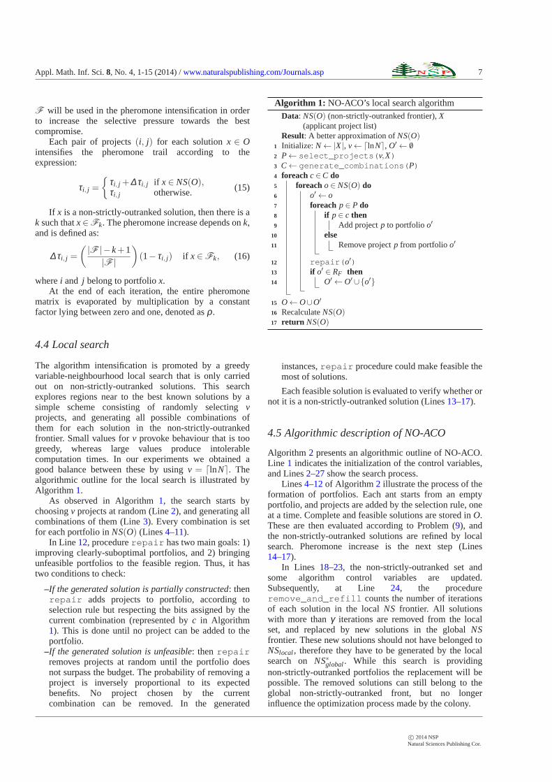
Appl. Math. Inf. Sci.8, No. 4, 1-15 (2014) /www.naturalspublishing.com/Journals.asp 7
F will be used in the pheromone intensification in orderto increase the selective pressure towards the bestcompromise.
Each pair of projects(i, j) for each solutionx ∈ Ointensifies the pheromone trail according to theexpression:
τi, j =
τi, j +∆τi, j if x∈ NS(O),τi, j otherwise. (15)
If x is a non-strictly-outranked solution, then there is ak such thatx∈Fk. The pheromone increase depends onk,and is defined as:
∆τi, j =
(
|F |−k+1|F |
)
(1− τi, j) if x∈Fk, (16)
wherei and j belong to portfoliox.At the end of each iteration, the entire pheromone
matrix is evaporated by multiplication by a constantfactor lying between zero and one, denoted asρ .
4.4 Local search
The algorithm intensification is promoted by a greedyvariable-neighbourhood local search that is only carriedout on non-strictly-outranked solutions. This searchexplores regions near to the best known solutions by asimple scheme consisting of randomly selectingvprojects, and generating all possible combinations ofthem for each solution in the non-strictly-outrankedfrontier. Small values forv provoke behaviour that is toogreedy, whereas large values produce intolerablecomputation times. In our experiments we obtained agood balance between these by usingv = ⌈lnN⌉. Thealgorithmic outline for the local search is illustrated byAlgorithm 1.
As observed in Algorithm1, the search starts bychoosingv projects at random (Line2), and generating allcombinations of them (Line3). Every combination is setfor each portfolio inNS(O) (Lines4–11).
In Line 12, procedurerepair has two main goals: 1)improving clearly-suboptimal portfolios, and 2) bringingunfeasible portfolios to the feasible region. Thus, it hastwo conditions to check:
–If the generated solution is partially constructed: thenrepair adds projects to portfolio, according toselection rule but respecting the bits assigned by thecurrent combination (represented byc in Algorithm1). This is done until no project can be added to theportfolio.
–If the generated solution is unfeasible: thenrepairremoves projects at random until the portfolio doesnot surpass the budget. The probability of removing aproject is inversely proportional to its expectedbenefits. No project chosen by the currentcombination can be removed. In the generated
Algorithm 1: NO-ACO’s local search algorithmData: NS(O) (non-strictly-outranked frontier),X
(applicant project list)Result: A better approximation ofNS(O)
1 Initialize: N← |X|, v← ⌈lnN⌉, O′← /02 P← select_projects(v,X)3 C← generate_combinations(P)4 foreachc∈C do5 foreacho∈ NS(O) do6 o′← o7 foreach p∈ P do8 if p∈ c then9 Add projectp to portfolioo′
10 else11 Remove projectp from portfolioo′
12 repair(o′)13 if o′ ∈ RF then14 O′←O′∪o′
15 O←O∪O′
16 RecalculateNS(O)17 return NS(O)
instances,repair procedure could make feasible themost of solutions.
Each feasible solution is evaluated to verify whether ornot it is a non-strictly-outranked solution (Lines13–17).
4.5 Algorithmic description of NO-ACO
Algorithm 2 presents an algorithmic outline of NO-ACO.Line 1 indicates the initialization of the control variables,and Lines2–27show the search process.
Lines4–12of Algorithm 2 illustrate the process of theformation of portfolios. Each ant starts from an emptyportfolio, and projects are added by the selection rule, oneat a time. Complete and feasible solutions are stored inO.These are then evaluated according to Problem (9), andthe non-strictly-outranked solutions are refined by localsearch. Pheromone increase is the next step (Lines14–17).
In Lines 18–23, the non-strictly-outranked set andsome algorithm control variables are updated.Subsequently, at Line 24, the procedureremove_and_refill counts the number of iterationsof each solution in the localNS frontier. All solutionswith more thanγ iterations are removed from the localset, and replaced by new solutions in the globalNSfrontier. These new solutions should not have belonged toNSlocal, therefore they have to be generated by the localsearch on NS∗global. While this search is providingnon-strictly-outranked portfolios the replacement will bepossible. The removed solutions can still belong to theglobal non-strictly-outranked front, but no longerinfluence the optimization process made by the colony.
c© 2014 NSPNatural Sciences Publishing Cor.

8 L. Cruz et. al. : Many-Objective Portfolio Optimization of Interdependent...
Algorithm 2: Non-Outranked Ant Colony Optimization algorithmData: X (applicant project list),B (budget)Result: An approximation ofNS(O)
1 Initialize: iter← 1, rep← 0, NSlocal← /0, NSglobal← /0, NS∗local← /02 repeat3 O← /04 foreachant in the colonydo5 x← make_empty_portfolio()6 X⊖← get_candidate_projects(X,x) // Section 4.27 repeat8 j ← selection_Rule(X⊖,x) // Equation (14)9 x j ← 1
10 X⊖← get_candidate_projects(X,x) // Section 4.211 until X⊖ = /012 O←O∪x
13 O←O∪NSlocal14 NSlocal← arg minx∈O〈|S(O,x)|, |W(O,x)|, |F(O,x)|〉 // Problem (9)15 NSlocal← local_search(NSlocal,X) // Algorithm 116 foreachx∈ NSlocal do17 lay_pheromone(x,O) // Equations (15-16)
18 NS∗global← NSglobal∪NSlocal
19 NS∗global← local_search(NS∗global,X) // Algorithm 1
20 if NSglobal = NS∗global then21 rep← rep+122 else23 rep← 0
24 remove_and_refill(NSlocal,NS∗global,γ)25 Evaporate pheromone // Section 4.326 Update:iter← iter+1,NSglobal← NS∗global
27 until rep= repmax∨ iter = itermax28 return NSglobal
At the end of each iteration, pheromone is evaporated(Line 25), and the remaining algorithm control variablesare updated (Line26). The algorithm finishes when it hasiterated with the same set of solutions as thenon-strictly-outranked frontier duringrepmax iterations,or if it has reached the maximum number of iterationsitermax (Line 27).
5 Case study: Optimization of socialassistance portfolios
Consider a DM facing a portfolio problem, with 100project proposals are aimed at benefitting the mostprecarious social classes. The project quality is measuredas the number of beneficiaries for each of nine criteriathat have previously been established. Each objective isassociated with one of three classes (extreme poverty,lower class and lower-middle class) and one of threelevels of impact (low, medium and high).
The total budget to distribute is 250 million dollars.The proposals can be grouped into three types accordingto their nature, and into two geographic regions according
to the location of their impact. Furthermore, in a desire toprovide equitable conditions, the DM imposes thefollowing restrictions:
1.The budget allocated to support each project typeshould be between 20% and 60% of the total budget.
2.The financial support allocated to each region must beat least 30% of the total budget, and no more than 70%.
The DM has also identified 20 relevant interactionsamong projects: four of them are cannibalizationphenomena, six correspond to situations ofmutually-excluding projects, and ten are synergisminteractions. There are up to five projects per interaction.
In order to make easier the comparative descriptions, inthis section the termPareto efficiency(and all the relatedterms, such asoptimal or efficient portfolio) will be usedto refer to non-dominated solutions of (1), and the termbest compromiseto best solutions to (9) (the best portfoliocompatible with the fuzzy outranking relation [10,15]).
Below, we present a range of experiments to verifythe validity and advantages of our approach to solvingthis case study. They give evidence of the benefits ofincorporating the DM’s preferences during the
c© 2014 NSPNatural Sciences Publishing Cor.

Appl. Math. Inf. Sci.8, No. 4, 1-15 (2014) /www.naturalspublishing.com/Journals.asp 9
Table 1: Effect of preferences incorporation on the Pareto Ant Colony Optimization algorithmIn
sta
nce
AlgorithmTime
Size Non-dominated Solutions Obtainsof the solutions belonging the best
(seconds) solution in to compromiseset O1∪O2 NS(O1∪O2) in O1∪O2
1P-ACO 3448.07 2006 928 10P-ACO-P 536.66 15 15 10 X
2P-ACO 3470.29 2514 1295 7P-ACO-P 775.94 19 19 13 X
3P-ACO 3485.16 2456 280 13P-ACO-P 1112.49 34 34 17 X
4P-ACO 3591.27 2587 1392 10 X
P-ACO-P 734.58 38 37 19 X
5P-ACO 3525.85 2245 1165 10P-ACO-P 1035.85 21 21 15 X
6P-ACO 3496.68 2013 161 11P-ACO-P 855.68 18 18 10 X
7P-ACO 3549.55 2211 766 13 X
P-ACO-P 161.02 19 19 14 X
8P-ACO 3464.27 2285 1317 13P-ACO-P 1646.32 28 28 21 X
9P-ACO 3707.65 965 762 4 X
P-ACO-P 712.24 25 25 11 X
10P-ACO 3549.67 2255 1403 15 X
P-ACO-P 651.43 18 18 16 X
Note: O1 andO2 are the solution sets generated by P-ACO and P-ACO-P respectively.The best compromise is the best solution to Problem (9) onO1∪O2.
optimization process, and thus they also prove that ourapproach has good potential for solving realresource-allocation problems.
5.1 Effect of incorporating the DM’spreferences
To the best of our knowledge, the P-ACO algorithm [16]is the most relevant ant colony algorithm applied to solveproject portfolio selection. In order to appraise the effectof incorporating the DM’s preferences on amulti-objective optimization algorithm, we implementeda version of P-ACO that included the preferential modeldescribed in Section3.2. This adaptation was calledP-ACO with preferences (P-ACO-P). Instead ofapproximating the Pareto frontier defined by the ninemaximizing objectives of the problem, it searches for thebest compromise expressed by Problem (9). In order toreflect a credible decision situation, we assign the valuessuggested by Fernandez et al. in [15] to the preferentialmodel parameters. There is no other difference betweenP-ACO and P-ACO-P. Both algorithms were programmedin Java language, using the JDK 1.6 compiler, andNetBeans 6.9.1 as Integrated Development Environment(IDE). The experiments were run on a Mac Pro with anIntel Quad-Core 2.8 GHz processor and 3 GB of RAM.
The P-ACO parameter setting was that suggested in[16] by Doerner et al. The version that incorporatespreferences has the same setting values.
Table1 shows the experimental results on ten artificialinstances following the case-study features.
The best compromise has been identified fromsolutions sets generated by both optimization methods. Inthis sense, that best compromise is related to the knownsolution set; therefore, it will be called theknown bestcompromise, which approximates the true bestcompromise. This is a non-dominated solution of Problem(9) on the original objective space. So, the true bestcompromise must belong to the true efficient set, and itshould not be strictly outranked by any other Paretosolution.
As can be seen from Table1, incorporatingpreferences provides a closer approximation to aprivileged region of the Pareto frontier. The versionconsidering preferences provides solutions thatdominated the 54%, on average, of solutions produced bythe original version of the algorithm. Probably, with manyobjectives, P-ACO is sensitive to the existence ofdominant resistant solutions. There is also a significantrun-time reduction (in the test cases, this reduction was76% on average). Also, if the model of preferencesmatches with the DM’s preferences, the best compromiseamong the set of all portfolios generated is alwaysidentified by P-ACO-P. Furthermore, when the DM has to
c© 2014 NSPNatural Sciences Publishing Cor.
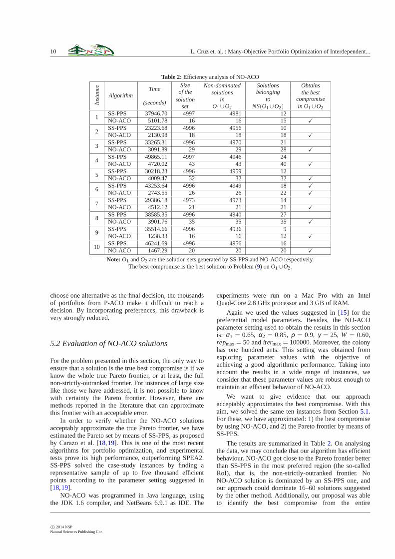
10 L. Cruz et. al. : Many-Objective Portfolio Optimization of Interdependent...
Table 2: Efficiency analysis of NO-ACO
Inst
an
ceAlgorithm
TimeSize Non-dominated Solutions Obtains
of the solutions belonging the best
(seconds) solution in to compromiseset O1∪O2 NS(O1∪O2) in O1∪O2
1SS-PPS 37946.70 4997 4981 12NO-ACO 5101.78 16 16 15 X
2SS-PPS 23223.68 4996 4956 10NO-ACO 2130.98 18 18 18 X
3SS-PPS 33265.31 4996 4970 21NO-ACO 3091.89 29 29 28 X
4SS-PPS 49865.11 4997 4946 24NO-ACO 4720.02 43 43 40 X
5SS-PPS 30218.23 4996 4959 12NO-ACO 4009.47 32 32 32 X
6SS-PPS 43253.64 4996 4949 18 X
NO-ACO 2743.55 26 26 22 X
7SS-PPS 29386.18 4973 4973 14NO-ACO 4512.12 21 21 21 X
8SS-PPS 38585.35 4996 4940 27NO-ACO 3901.76 35 35 35 X
9SS-PPS 35514.66 4996 4936 9NO-ACO 1238.33 16 16 12 X
10SS-PPS 46241.69 4996 4956 16NO-ACO 1467.29 20 20 20 X
Note: O1 andO2 are the solution sets generated by SS-PPS and NO-ACO respectively.The best compromise is the best solution to Problem (9) onO1∪O2.
choose one alternative as the final decision, the thousandsof portfolios from P-ACO make it difficult to reach adecision. By incorporating preferences, this drawback isvery strongly reduced.
5.2 Evaluation of NO-ACO solutions
For the problem presented in this section, the only way toensure that a solution is the true best compromise is if weknow the whole true Pareto frontier, or at least, the fullnon-strictly-outranked frontier. For instances of large sizelike those we have addressed, it is not possible to knowwith certainty the Pareto frontier. However, there aremethods reported in the literature that can approximatethis frontier with an acceptable error.
In order to verify whether the NO-ACO solutionsacceptably approximate the true Pareto frontier, we haveestimated the Pareto set by means of SS-PPS, as proposedby Carazo et al. [18,19]. This is one of the most recentalgorithms for portfolio optimization, and experimentaltests prove its high performance, outperforming SPEA2.SS-PPS solved the case-study instances by finding arepresentative sample of up to five thousand efficientpoints according to the parameter setting suggested in[18,19].
NO-ACO was programmed in Java language, usingthe JDK 1.6 compiler, and NetBeans 6.9.1 as IDE. The
experiments were run on a Mac Pro with an IntelQuad-Core 2.8 GHz processor and 3 GB of RAM.
Again we used the values suggested in [15] for thepreferential model parameters. Besides, the NO-ACOparameter setting used to obtain the results in this sectionis: α1 = 0.65, α2 = 0.85, ρ = 0.9, γ = 25, W = 0.60,repmax= 50 anditermax= 100000. Moreover, the colonyhas one hundred ants. This setting was obtained fromexploring parameter values with the objective ofachieving a good algorithmic performance. Taking intoaccount the results in a wide range of instances, weconsider that these parameter values are robust enough tomaintain an efficient behavior of NO-ACO.
We want to give evidence that our approachacceptably approximates the best compromise. With thisaim, we solved the same ten instances from Section5.1.For these, we have approximated: 1) the best compromiseby using NO-ACO, and 2) the Pareto frontier by means ofSS-PPS.
The results are summarized in Table2. On analysingthe data, we may conclude that our algorithm has efficientbehaviour. NO-ACO got close to the Pareto frontier betterthan SS-PPS in the most preferred region (the so-calledRoI), that is, the non-strictly-outranked frontier. NoNO-ACO solution is dominated by an SS-PPS one, andour approach could dominate 16–60 solutions suggestedby the other method. Additionally, our proposal was ableto identify the best compromise from the entire
c© 2014 NSPNatural Sciences Publishing Cor.
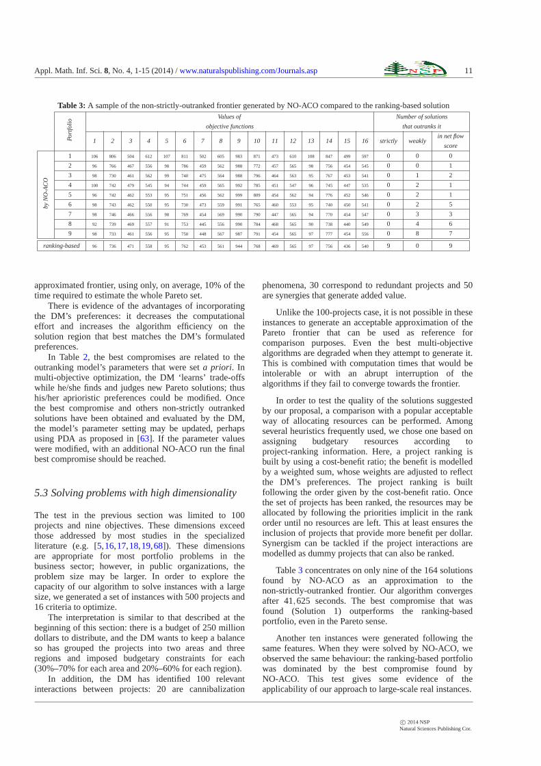
Appl. Math. Inf. Sci.8, No. 4, 1-15 (2014) /www.naturalspublishing.com/Journals.asp 11
Table 3: A sample of the non-strictly-outranked frontier generated by NO-ACO compared to the ranking-based solution
Port
folio
Values of Number of solutions
objective functions that outranks it
1 2 3 4 5 6 7 8 9 10 11 12 13 14 15 16 strictly weaklyin net flow
score
by
NO
-AC
O
1 106 806 504 612 107 811 502 605 983 871 473 610 108 847 499 597 0 0 0
2 96 766 467 556 98 786 459 562 988 772 457 565 98 756 454 545 0 0 1
3 98 730 461 562 99 740 475 564 988 796 464 563 95 767 453 541 0 1 2
4 100 742 479 545 94 744 459 565 992 785 451 547 96 745 447 535 0 2 1
5 96 742 462 553 95 751 456 562 999 809 454 562 94 776 452 546 0 2 1
6 98 743 462 550 95 730 473 559 991 765 460 553 95 740 450 541 0 2 5
7 98 746 466 556 98 769 454 569 990 790 447 565 94 770 454 547 0 3 3
8 92 739 469 557 91 753 445 556 990 784 468 565 90 738 440 549 0 4 6
9 98 733 461 556 95 750 448 567 987 791 454 565 97 777 454 556 0 8 7
ranking-based 96 736 471 558 95 762 453 561 944 768 469 565 97 756 436 540 9 0 9
approximated frontier, using only, on average, 10% of thetime required to estimate the whole Pareto set.
There is evidence of the advantages of incorporatingthe DM’s preferences: it decreases the computationaleffort and increases the algorithm efficiency on thesolution region that best matches the DM’s formulatedpreferences.
In Table 2, the best compromises are related to theoutranking model’s parameters that were seta priori. Inmulti-objective optimization, the DM ‘learns’ trade-offswhile he/she finds and judges new Pareto solutions; thushis/her aprioristic preferences could be modified. Oncethe best compromise and others non-strictly outrankedsolutions have been obtained and evaluated by the DM,the model’s parameter setting may be updated, perhapsusing PDA as proposed in [63]. If the parameter valueswere modified, with an additional NO-ACO run the finalbest compromise should be reached.
5.3 Solving problems with high dimensionality
The test in the previous section was limited to 100projects and nine objectives. These dimensions exceedthose addressed by most studies in the specializedliterature (e.g. [5,16,17,18,19,68]). These dimensionsare appropriate for most portfolio problems in thebusiness sector; however, in public organizations, theproblem size may be larger. In order to explore thecapacity of our algorithm to solve instances with a largesize, we generated a set of instances with 500 projects and16 criteria to optimize.
The interpretation is similar to that described at thebeginning of this section: there is a budget of 250 milliondollars to distribute, and the DM wants to keep a balanceso has grouped the projects into two areas and threeregions and imposed budgetary constraints for each(30%–70% for each area and 20%–60% for each region).
In addition, the DM has identified 100 relevantinteractions between projects: 20 are cannibalization
phenomena, 30 correspond to redundant projects and 50are synergies that generate added value.
Unlike the 100-projects case, it is not possible in theseinstances to generate an acceptable approximation of thePareto frontier that can be used as reference forcomparison purposes. Even the best multi-objectivealgorithms are degraded when they attempt to generate it.This is combined with computation times that would beintolerable or with an abrupt interruption of thealgorithms if they fail to converge towards the frontier.
In order to test the quality of the solutions suggestedby our proposal, a comparison with a popular acceptableway of allocating resources can be performed. Amongseveral heuristics frequently used, we chose one based onassigning budgetary resources according toproject-ranking information. Here, a project ranking isbuilt by using a cost-benefit ratio; the benefit is modelledby a weighted sum, whose weights are adjusted to reflectthe DM’s preferences. The project ranking is builtfollowing the order given by the cost-benefit ratio. Oncethe set of projects has been ranked, the resources may beallocated by following the priorities implicit in the rankorder until no resources are left. This at least ensures theinclusion of projects that provide more benefit per dollar.Synergism can be tackled if the project interactions aremodelled as dummy projects that can also be ranked.
Table3 concentrates on only nine of the 164 solutionsfound by NO-ACO as an approximation to thenon-strictly-outranked frontier. Our algorithm convergesafter 41,625 seconds. The best compromise that wasfound (Solution 1) outperforms the ranking-basedportfolio, even in the Pareto sense.
Another ten instances were generated following thesame features. When they were solved by NO-ACO, weobserved the same behaviour: the ranking-based portfoliowas dominated by the best compromise found byNO-ACO. This test gives some evidence of theapplicability of our approach to large-scale real instances.
c© 2014 NSPNatural Sciences Publishing Cor.
12 L. Cruz et. al. : Many-Objective Portfolio Optimization of Interdependent...
6 Conclusions and future work
We have presented an original proposal to optimizeinterdependent projects portfolios. This proposal is anadaptation of the well-known ant colony optimizationmetaheuristic, but incorporates preferences based on theoutranking model of Fernandez et al. [10]. Our algorithm(NO-ACO) searches for optimal portfolios in synergeticconditions and can handle interactions impacting bothobjectives and costs. Redundancy is also consideredduring portfolio formation. By incorporating preferences,the selective pressure toward a privileged zone of thePareto frontier is increased. Thus, a zone that matches theDM’s preferences better can be identified. In comparisonwith other metaheuristic approach that does notincorporate preferences, NO-ACO achieves greatercloseness to the region of interest with less computationaleffort. Our result seems to confirm the hypothesis from[10,15]: the incorporation of DM preferences by solvingProblem (9) helps to obtain solutions that dominate othersfrom leading metaheuristics.
Since it is enriched by preferences, our proposalacquires the ability to find good solutions (the known bestportfolio) to portfolio problems with higher dimensions(in project and objective spaces) than those reported inscientific literature. Compared to the popularranking-based method, NO-ACO finds solutions thatoutperform to the ranking-based portfolio, both in Paretodominance and in strict outranking.
As immediate work we are going to explore the limitsof this approach, by finding the greatest size of theinstances that can be solved with an acceptableperformance. Additionally, we are going to incorporate aninteractive process for updating the preference modelaccording to the new information gained by the DM fromthe optimized solutions.
Acknowledgements
We acknowledge the support from PROMEP through thenetwork project ‘Optimization and Decision Support’. Wealso thank to DGEST and the Autonomous University ofSinaloa (PROFAPI-055/2012 project).
References
[1] D N Kleinmuntz. Portfolio Decision Analysis: Improvedmethods for resource allocation, chapter Foreword, pagesv–vii. Springer, New York-Dordrecht-Heidelberg-London,2011.
[2] A Salo, J Keisler, and A Morton. Portfolio DecisionAnalysis: Improved methods for resource allocation, chapterAn invitation to Portfolio Decision Analysis, pages 3–27.Springer, New York-Dordrecht-Heidelberg-London, 2011.
[3] M A Coffin and B W Taylor. Multiple criteria R&D projectselection and scheduling using fuzzy sets.Comput Oper Res,23(3):207–220, 1996.
[4] J Klapka, P Pinos, and V Sevcik. Multicriterial projectsselection. Handbook of Optimization, Intelligent SystemsReference Library, 38:245–261, 2013.
[5] C Stummer and K Heidenberger. Interactive R&D portfolioanalysis with project interdependencies and timeprofiles ofmultiple objectives. IEEE T Eng Manage, 50(2):175–183,2003.
[6] J L Ringuest, S B Graves, and Case R H. Mean-gini analysisin R&D portfolio selection.Eur J Oper Res, 154(1):157–169,2004.
[7] C Carlsson, R Fuller, M Heikkila, and Majlender P. Adynamic and fuzzy modeling approach for multi-objectiveR&D project portfolio selection. Int J Approx Reason,44(2):93–105, 2007.
[8] X Zhao, Y Yang, G Wu, J Yang, and X Xue. A dynamic andfuzzy modeling approach for multi-objective R&D projectportfolio selection.J Converg Inf Technol, 7(1):36–44, 2012.
[9] W Hallerbach, H Ning, A Soppe, and J Spronk. A frameworkfor managing a portfolio of socially responsible investments.Eur J Oper Res, 153(2):517–529, 2004.
[10] E Fernandez, E Lopez, G Mazcorro, R Olmedo, and C ACoello Coello. Application of the Non-Outranked SortingGenetic Algorithm to public project portfolio selection.InfSci, 228:131–149, 2013.
[11] Georgia Department of Transportation. project list andfinal investment report. available in http:// www.dot.ga.gov/localgovernment/ fundingprograms/ transreferendum/pages/projectlist.aspx (october 4th, 2012).
[12] Georgia Department of Transportation. Central SavannahRiver Area, unconstrained project list by county. availablein http:// www.it3.ga.gov/ documents/ unconstrainedlist/centralsavannah-unconstrainedlist.pdf (october 4th, 2012).
[13] Georgia Department of Transportation. Heart of Georgia,Altamaha unconstrained project list by county. availablein http:// www.it3.ga.gov/ documents/ unconstrainedlist/heartofgeorgia-unconstrainedlist-fullset.pdf (october 4th,2012).
[14] Georgia Department of Transportation. River Valley Area,unconstrained project list by county. available in http://www.it3.ga.gov/ documents/ unconstrainedlist/ rivervalley-unconstrainedlist.pdf (october 4th, 2012).
[15] E Fernandez, E Lopez, F Lopez, and C A Coello Coello.Increasing selective pressure towards the best compromisein evolutionary multiobjective optimization: The extendedNOSGA method.Inf Sci, 181(1):44–56, 2011.
[16] K F Doerner, W J Gutjahr, R F Hartl, C Strauss, andC Stummer. Pareto Ant Colony optimization: A metaheuristicapproach to multiobjective portfolio selection.Ann Oper Res,131(1–4):79–99, 2004.
[17] K F Doerner, W J Gutjahr, R Hartl, C Strauss, andC Stummer. Pareto Ant Colony Optimization with ILPpreprocessing in multiobjective project portfolio selection.Eur J Oper Res, 171(3):830–841, 2006.
[18] A F Carazo, T Gomez, J Molina, A G Hernández-Díaz, F MGuerrero, and R Caballero. Solving a comprehensive modelfor multiobjective project portfolio selection.Comput OperRes, 37(4):630–639, 2010.
[19] A F Carazo, I Contreras, T Gomez, and F Perez. Aproject portfolio selection problem in a group decision-making context.J Ind Manage Optim, 8(1):243–261, 2012.
c© 2014 NSPNatural Sciences Publishing Cor.

Appl. Math. Inf. Sci.8, No. 4, 1-15 (2014) /www.naturalspublishing.com/Journals.asp 13
[20] C L Hwang and A S M Masud. Multiple objectivedecision making, methods and applications: a state-of-the-art survey. Lecture notes in economics and mathematicalsystems. Springer-Verlag, 1979.
[21] F Ghasemzadeh, N Archer, and P Iyogun. A zero-one modelfor project portfolio selection and scheduling.J Oper ResSoc, 50(7):745–755, 1999.
[22] B Amiri. A multi-objective hybrid optimization algorithmfor project selection problem. J Basic Appl Sci Res,2(7):6995–7002, 2012.
[23] T Kremmel, J Kubalik, and S Biffl. Softwareproject portfolio optimization with advanced multi-objectiveevolutionary algorithm.Appl Soft Comput, 11(1):1416–1426,2011.
[24] A Chen and Ch Chyu. Applying memetic algorithmin multi-objective resource allocation among competingprojects.J Softw, 5(8):802–809, 2010.
[25] J Gaytán and J García. Multicriteria decision oninterdependent infrastructure transportation projects using anevolutionary-based framework.Appl Soft Comput, 9(2):512–526, 2009.
[26] S Ghorbani and M Rabbani. A new multi-objectivealgorithm for a project selection problem.Adv Eng Softw,40(1):9–14, 2009.
[27] C M Lin and M Gen. Multicriteria human resourceallocation for solving multistage combinatorial optimizationproblems using multiobjective hybrid genetic algorithm.Expert Syst Appl, 34(4):2480–2490, 2008.
[28] W J Gutjahr, S Katzensteiner, P Reiter, C Stummer, andM Denk. Multi-objective decision analysis for competence-oriented project portfolio selection. Eur J Oper Res,205(3):670–679, 2010.
[29] E Zitzler, M Laumanns, and L Thiele. SPEA2: Improvingthe strength pareto evolutionary algorithm. Technical Report103, Computer Engineering and Networks Laboratory (TIK),Swiss Federal Institute of Technology (ETH), 2001.
[30] H Ishibuchi, N Tsukamoto, and Y Nojima. Evolutionarymany-objective optimization: A short review. InProceedingsof Evolutionary Computation, 2008 (CEC’2008), pages2419–2426. IEEE, 2008.
[31] D W Corne and J D Knowles. Techniques for highlymultiobjective optimisation: some nondominated points arebetter than others. InProceedings of the 9th annualconference on Genetic and evolutionary computation,GECCO’07, pages 773–780, New York, NY, USA, 2007.
[32] J López, C A COello Coello, K Oyama, and FujiiK. Alternative preference relation to deal with many-objective optimization problems. In R C Purshouse, P JFleming, C M Fonseca, S Greco, and J Shaw, editors,Proceedings of Evolutionary Multi-Criterion Optimization -EMO 2013, Lecture Notes in Computer Science, pages 291–306. Springer-Verlag, 2013.
[33] R C Purshouse and P J Fleming. Evolutionary many-objective optimisation: An exploratory analysis. InEvolutionary Computation, 2003. CEC’03. The 2003Congress on, volume 3, pages 2066–2073. IEEE, 2003.
[34] S Huband, L Barone, P Hingston, While R L,D Tuppurainen, and R Bearman. Designing comminutioncircuits with a multi-objective evolutionary algorithm. InCongress on Evolutionary Computation, pages 1815–1822,2005.
[35] G A Miller. The magical number seven, plus or minustwo: some limits on our capacity for processing information.Psychological Review, 63(2):81–97, 1956.
[36] K Deb, J Sundar, U Bhaskara, and S Chaudhuri. Referencepoint based multiobjective optimization using evolutionaryalgorithms.Int J Comput Intell Res, 2(3):273–286, 2006.
[37] S Bechikh. Incorporating Decision Maker’s PreferenceInformation in Evolutionary Multi-objective Optimization.PhD thesis, High Institute of Management of Tunis,University of Tunis, Tunis, Tunisia, 2013.
[38] K Deb. Multi-objective evolutionary algorithms:Introducing bias among pareto optimal solutions. TechnicalReport KanGAL Report 99002, Indian Institute ofTechnology, Kanpur, India, 1999.
[39] J Branke and K Deb. Knowledge Incorporationin Evolutionary Computation, chapter Integrating userpreferences into evolutionary multi-objective optimization,pages 461–478. Springer-Verlag, Berlin-Heidelberg, 2004.
[40] E Zitzler, D Brockhoff, and L Thiele. The hypervolumeindicator revisited: On the design of pareto-compliantindicators via weighted integration. InProceedings of the4th international conference on Evolutionary Multi-criterionOptimization (EMO’07), pages 862–876, Matsushima, Japan,2007. Springer-Verlag.
[41] G W Greenwood, X S Hu, and J C D’ambrosio.Foundationsof Genetic Algorithms, chapter Fitness functions for multipleobjective optimization problems: combining preferences withPareto rankings, pages 437–455. Morgan Kaufmann, 1996.
[42] K Deb, A Sinha, P Korhonen, and J Wallenius. Aninteractive evolutionary multiobjective optimization methodbased on progressively approximated value functions.IEEET Evolut Comput, 14(5):723–739, 2010.
[43] M Köksalan and I Karahan. An interactive territory definingevolutionary algorithm: itdea.Evolut Comput, 14(5):702–722, 2010.
[44] R Battiti and A Passerini. Brain-computer evolutionarymultiobjective optimization: A genetic algorithm adapting tothe decision maker.IEEE T Evolut Comput, 14(5):671–687,2010.
[45] J W Fowler, ES Gel, M Köksalan, P Korhonen, J L Marquis,and J Wallenius. Interactive evolutionary multi-objectiveoptimization for quasi-concave preference functions.IEEET Evolut Comput, 206(2):417–425, 2010.
[46] J Branke, S Greco, R Slowinski, and P Zielniewski.Interactive evolutionary multiobjective optimization drivenby robust ordinal regression.Bull Polish Acad Sci, 58(3):347–358, 2010.
[47] Y C Jin and B Sendhoff. Incorporation of fuzzypreferences into evolutionary multiobjective optimization. InProceedings of the 4th Asia-Pacific conference on SimulatedEvolution and Learning, Nanyang, Singapore, 2002.
[48] D Cvetkovic and I C Parmee. Preferences and theirapplication in evolutionary multiobjectiveoptimisation.IEEET Evolut Comput, 6(1):42–57, 2002.
[49] L Rachmawati and D Srinivasan. Incorporating thenotion of relative importance of objectives in evolutionarymultiobjective optimization. IEEE T Evolut Comput 2010,14(4):530–546, 2010.
[50] K Deb and A Kumar. Interactive evolutionary multi-objective optimization and decision making using referencedirection method. InProceedings of the 9th Genetic and
c© 2014 NSPNatural Sciences Publishing Cor.
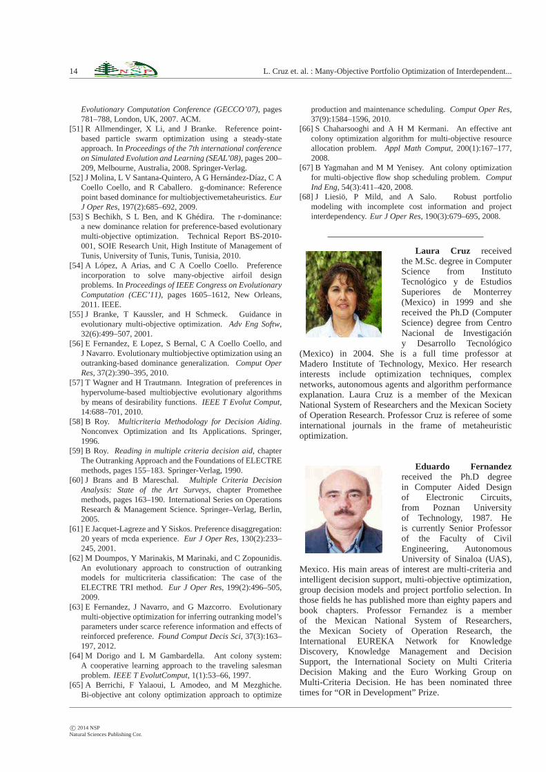
14 L. Cruz et. al. : Many-Objective Portfolio Optimization of Interdependent...
Evolutionary Computation Conference (GECCO’07), pages781–788, London, UK, 2007. ACM.
[51] R Allmendinger, X Li, and J Branke. Reference point-based particle swarm optimization using a steady-stateapproach. InProceedings of the 7th international conferenceon Simulated Evolution and Learning (SEAL’08), pages 200–209, Melbourne, Australia, 2008. Springer-Verlag.
[52] J Molina, L V Santana-Quintero, A G Hernández-Díaz, C ACoello Coello, and R Caballero. g-dominance: Referencepoint based dominance for multiobjectivemetaheuristics.EurJ Oper Res, 197(2):685–692, 2009.
[53] S Bechikh, S L Ben, and K Ghédira. The r-dominance:a new dominance relation for preference-based evolutionarymulti-objective optimization. Technical Report BS-2010-001, SOIE Research Unit, High Institute of Management ofTunis, University of Tunis, Tunis, Tunisia, 2010.
[54] A López, A Arias, and C A Coello Coello. Preferenceincorporation to solve many-objective airfoil designproblems. InProceedings of IEEE Congress on EvolutionaryComputation (CEC’11), pages 1605–1612, New Orleans,2011. IEEE.
[55] J Branke, T Kaussler, and H Schmeck. Guidance inevolutionary multi-objective optimization.Adv Eng Softw,32(6):499–507, 2001.
[56] E Fernandez, E Lopez, S Bernal, C A Coello Coello, andJ Navarro. Evolutionary multiobjective optimization using anoutranking-based dominance generalization.Comput OperRes, 37(2):390–395, 2010.
[57] T Wagner and H Trautmann. Integration of preferences inhypervolume-based multiobjective evolutionary algorithmsby means of desirability functions.IEEE T Evolut Comput,14:688–701, 2010.
[58] B Roy. Multicriteria Methodology for Decision Aiding.Nonconvex Optimization and Its Applications. Springer,1996.
[59] B Roy. Reading in multiple criteria decision aid, chapterThe Outranking Approach and the Foundations of ELECTREmethods, pages 155–183. Springer-Verlag, 1990.
[60] J Brans and B Mareschal. Multiple Criteria DecisionAnalysis: State of the Art Surveys, chapter Prometheemethods, pages 163–190. International Series on OperationsResearch & Management Science. Springer–Verlag, Berlin,2005.
[61] E Jacquet-Lagreze and Y Siskos. Preference disaggregation:20 years of mcda experience.Eur J Oper Res, 130(2):233–245, 2001.
[62] M Doumpos, Y Marinakis, M Marinaki, and C Zopounidis.An evolutionary approach to construction of outrankingmodels for multicriteria classification: The case of theELECTRE TRI method.Eur J Oper Res, 199(2):496–505,2009.
[63] E Fernandez, J Navarro, and G Mazcorro. Evolutionarymulti-objective optimization for inferring outranking model’sparameters under scarce reference information and effects ofreinforced preference.Found Comput Decis Sci, 37(3):163–197, 2012.
[64] M Dorigo and L M Gambardella. Ant colony system:A cooperative learning approach to the traveling salesmanproblem.IEEE T EvolutComput, 1(1):53–66, 1997.
[65] A Berrichi, F Yalaoui, L Amodeo, and M Mezghiche.Bi-objective ant colony optimization approach to optimize
production and maintenance scheduling.Comput Oper Res,37(9):1584–1596, 2010.
[66] S Chaharsooghi and A H M Kermani. An effective antcolony optimization algorithm for multi-objective resourceallocation problem. Appl Math Comput, 200(1):167–177,2008.
[67] B Yagmahan and M M Yenisey. Ant colony optimizationfor multi-objective flow shop scheduling problem.ComputInd Eng, 54(3):411–420, 2008.
[68] J Liesiö, P Mild, and A Salo. Robust portfoliomodeling with incomplete cost information and projectinterdependency.Eur J Oper Res, 190(3):679–695, 2008.
Laura Cruz receivedthe M.Sc. degree in ComputerScience from InstitutoTecnológico y de EstudiosSuperiores de Monterrey(Mexico) in 1999 and shereceived the Ph.D (ComputerScience) degree from CentroNacional de Investigacióny Desarrollo Tecnológico
(Mexico) in 2004. She is a full time professor atMadero Institute of Technology, Mexico. Her researchinterests include optimization techniques, complexnetworks, autonomous agents and algorithm performanceexplanation. Laura Cruz is a member of the MexicanNational System of Researchers and the Mexican Societyof Operation Research. Professor Cruz is referee of someinternational journals in the frame of metaheuristicoptimization.
Eduardo Fernandezreceived the Ph.D degreein Computer Aided Designof Electronic Circuits,from Poznan Universityof Technology, 1987. Heis currently Senior Professorof the Faculty of CivilEngineering, AutonomousUniversity of Sinaloa (UAS),
Mexico. His main areas of interest are multi-criteria andintelligent decision support, multi-objective optimization,group decision models and project portfolio selection. Inthose fields he has published more than eighty papers andbook chapters. Professor Fernandez is a memberof the Mexican National System of Researchers,the Mexican Society of Operation Research, theInternational EUREKA Network for KnowledgeDiscovery, Knowledge Management and DecisionSupport, the International Society on Multi CriteriaDecision Making and the Euro Working Group onMulti-Criteria Decision. He has been nominated threetimes for “OR in Development” Prize.
c© 2014 NSPNatural Sciences Publishing Cor.
Appl. Math. Inf. Sci.8, No. 4, 1-15 (2014) /www.naturalspublishing.com/Journals.asp 15
Claudia Gomezwas bornin Mexico in 1971. She is afull time professor at MaderoInstitute of Technology. Shereceived the Ph.D degree inAdvanced Technology fromNational Polytechnic Institute(Mexico), in 2009. Shereceived the M.Sc. degree inComputer Science from Leon
Institute of Technology (Mexico), in 2000. Her researchinterests are optimization techniques, complex networkand autonomous agents.
Gilberto Riverawas born in Mexico in1984. He is a Ph.D studentat Inter-institutional Networkof Tijuana-Madero-and-LeonIntitutes of Technology.He received the M.Sc.degree in Computer Sciencefrom Madero Instituteof Technology (Mexico),in 2010. His research interests
are in the areas of project portfolio selection, optimizationtechniques, swarm intelligence and autonomous agents.
Fatima Perez is aResearch Fellow at Universityof Malaga (Spain). Shereceived the Ph.D degree inMathematical Economics atUniversity of Malaga. She haspublished research articles inreputed international journalsin the frame of appliedmathematics and applied
economics. Her research interests are in the areas ofproject portfolio selection, multiobjective programming,metaheuristic algorithms, development of computersoftware and composite indicators. She is referee of someinternational journals in the frame of multiobjectiveprogramming.
c© 2014 NSPNatural Sciences Publishing Cor.