1

A Seismic Resistant Design Algorithm for Layingand Shielding of Optical Fiber Cables

Zengfu Wang, Qing Wang, Moshe Zukerman, Fellow, IEEE, Bill Moran

Abstract—This paper considers a long-haul optical fiber cable,connecting two points on the Earth’s surface that passes throughearthquake-prone or other sensitive areas. Different segments ofthe cable are characterized by different protection levels, where ahigher level through shielding represents a more costly and moreresilient segment. This leads to a multi-objective optimizationproblem where the two objectives are: (1) total cost of the cable,and (2) total number of potential repairs along the cable likelyto be caused by earthquakes. As a measure of seismic risk weuse the concept of cable repair rate used in the civil engineeringcommunity. In our models, ground motion intensity data are usedto estimate the cable repair rate, and a graph of a triangulatedirregular network is used to represent the Earth’s surface. Weformulate this optimization problem as a multi-objective shortestpath problem and solve it by a variant of the label settingalgorithm. Two approximate algorithms, an interval-partition-based label-setting algorithm and an evolutionary algorithm arealso presented as methods of computational cost reduction forlarge scale cases, and their results are compared. The solutionleads to a Pareto front or an approximate Pareto front thatenables us to choose the path and protection of the cable toeither minimize cost for a given risk level or minimize risk fora given budget.

Index Terms—Optical fiber cables, path optimization, multi-objective optimization, cost effectiveness, seismic resilience.

I. INTRODUCTION

Long-haul optical fiber cables, are vital for transporting in-formation critical for the operation of a modern society.According to the latest Submarine Cable Map updated byTeleGeography for 2016 [1], around 321 submarine telecom-munication cable systems (293 in-service and 28 planned) withmore than 550,000 miles carry over 99% of the internationalcommunications [2]. On the one hand, constructing such

The work described in this paper was primarily supported by a grantfrom the Research Grants Council of the Hong Kong Special AdministrativeRegion, China [Project No. CityU8/CRF/13G], and it was also supported by agrant from the National Natural Science Foundation of China (NSFC) [ProjectNo. 61503305], and by the Fundamental Research Funds for the CentralUniversities [Project No. 3102017zy025].

Z. Wang (Corresponding Author) is with the School of Automation,Northwestern Polytechnical University, Xi’an, PRC, and the Department ofElectronic Engineering, City University of Hong Kong, Kowloon, Hong KongSAR, PRC. (email: wangzengfu@gmail.com)

Q. Wang and M. Zukerman are with the Department of Electronic Engi-neering, City University of Hong Kong, Kowloon, Hong Kong SAR, PRC(email: qwang99-c@my.cityu.edu.hk; m.zu@cityu.edu.hk).

B. Moran is with the School of Engineering, RMIT University, Melbourne,Australia. (bill.moran@rmit.edu.au)

Copyright (c) 2015 IEEE. Personal use of this material is permitted.However, permission to use this material for any other purposes must beobtained from the IEEE by sending a request to pubs-permissions@ieee.org.

cables requires significant capital investment with a driveto minimize upfront costs. On the other hand, survivabilityunder various disasters is also of significant importance sincebreakages can have severe social, economic and financialconsequences.

A range of measures can be used to improve survivability ofan optical fiber cable; specifically, special shielding or extramaterial can be added to enhance the robustness of the cablepassing through high risk areas, or a path can be chosen thatavoids such areas, or a combination of these measures canbe used. This requirement is highlighted by the followingexample. In 2006, eight submarine telecommunication cables(APCN, APCN-2, C2C, China-US CN, EAC, FLAG FEA,FNAL/RNAL and SMW3) were damaged, with a total of18 cuts, by the Hengchun earthquake [3]. As a consequence,Internet services in several Asian countries/regions includingChina, Taiwan, Hong Kong etc., were severely disrupted forseveral weeks [3]. For a modern society, largely reliant onthe Internet, an Internet blackout for one week can lead toover 1% loss of annual GDP [4], [5]. Again in 2009, thesame eight cables were destroyed by the Ryukyu Islandsearthquake. However, TPE and TGN-IA, two new cables laidin 2008 and 2009, respectively, were not affected since theywere deliberately laid a safe distance away from the Taiwanearthquake prone area. As a result, the impact of the 2009earthquake was almost insignificant relative to that of the2006 earthquake [3]. Of course, the damaged cables had tobe repaired, but the consequences to users were minor.

In practice, there are several different approaches to cableshielding, expressed in terms of different protection levelsavailable for cables. For example, several types of submarinefiber cables with different strengths of the armor are availableand may be used in a submarine cable system according to thedepth of the seabed where the cable lies [6]. The constructioncost of a cable is an increasing function of the protection level,while the potential seismic damage is a decreasing function ofits protection level.

Because of the increased cost of higher protection level ofcables, it is important to identify the critical segments of thecable that are more likely to be damaged (for example, becausethey are located in higher risk areas), and strengthen thosesegments to increase overall cable survivability.

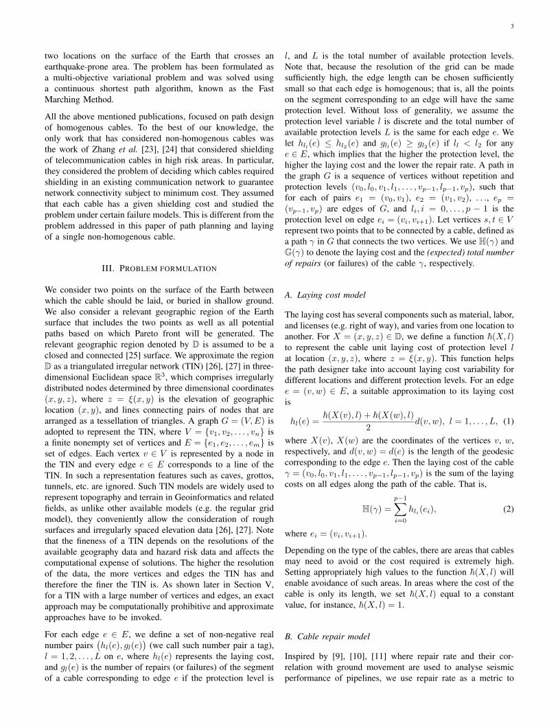
In this paper, we study the problem of optimizing the path andprotection level for an optical fiber cable connecting two siteson the Earths surface. For ease of exposition, throughout mostof this paper we only consider earthquake risks. However, in

2

Section VI, we explain how our approach can be applied toconsider other risks associated with cable laying that includenatural hazards other than earthquakes, and human activitiessuch as fishing, as well as to consider areas where cables can-not be laid, for example, areas where license for cables cannotbe obtained, or areas of high ecological values. Henceforth,we use the terms laying and construction interchangeably tomean either laying or construction of cables. The related termslaying costs include all direct and indirect costs associatedwith building, installing, laying and/or constructing the cable.These include cost of materials, labor used in cable production,transportation, licenses, etc.

For such a practically important problem, to the best of ourknowledge, there is no other solution based on a rigorousapproach or even a heuristic approach available in the lit-erature. To address this gap, we provide a formulation of amulti-objective shortest path problem, where we aim to obtainall Pareto optimal paths for the cable with the following twoobjective functions. The first objective is the laying cost of thecable based on the length of the cable and the costs associatedwith the various protection levels used in high risk areas.The second objective is the risk of cable failure, quantifiedas the number of potential repairs along the cable as a resultof earthquakes. This measure is commonly used in practice[7] as well as in the civil engineering literature [8] for thispurpose because, firstly, the number is associated with the costof reconstruction as well as business and societal costs of afailed cable and, secondly, it can be estimated from groundmotion data, from which we can obtain the cable repair rate[9], [10], [11].

We use a triangulated irregular network to approximate theEarth’s surface, and ground motion intensity measures ofearthquakes, obtained either from available data (e.g. USGS(https://www.usgs.gov/)), or by Probabilistic Seismic HazardAnalysis (PSHA) [12] to estimate the cable repair rate. Basedon this model, we solve the multi-objective shortest pathproblem by an extension of the known label setting algorithm.This enables us to obtain all the Pareto optimal solutionsthat provide considerable flexibility in cable route selection,taking into consideration the available protection levels and thetrade-off between cost effectiveness and seismic resilience. Forlarge scale path optimization problems with a huge numberof non-dominated labels, an interval-partition-based label-setting algorithm and an evolutionary algorithm are used toderive approximate solutions and their results are compared.In summary, our novelty here is twofold:

• We apply, apparently for the first time, a multiple-protection-level repair rate model based on ground motionintensities, a landform model based on a triangulatedirregular network, and a multiple-protection-level layingcost model for optimizing the path and non-homogenousconstruction of a cable.

• We apply the label setting algorithm to the multi-objectiveshortest path problem of minimizing laying cost whileminimizing total number of repairs, again apparently forthe first time.

The remainder of the paper is organized as follows. In SectionII, we discuss the state of the art and the related work. InSection III, we introduce models of laying costs and cablerepairs, and formulate the problem of minimizing layingcost and total number of repairs (a risk measure used inthis paper) for cable design considering path planning andmultiple protection levels. Next, leveraging on the label settingalgorithm [13], our path planning algorithm is given in SectionIV and two approximation algorithms are briefly introduced.In Section V, simulation results of the three algorithms basedon a 2D scenario and two real-world 3D data are presented.Then, in Section VI we discuss the extension of our approachto consider other hazardous and sensitive areas. In Section VIIwe give our conclusions from the work.

II. STATE OF THE ART AND RELATED WORK

Current approaches to path planning, or route selection forfiber optical cables between two locations, have focused onhomogenous cables where, in our context, the number ofprotection levels is equal to one. In practice, the path planningprocedures of cables have been implemented by traditionalmanual approach based on expert experience [7], [14].

In the traditional manual approach, using available data ina region of interest such as maps, aerial photographs etc.,planners provide several relatively reasonable paths on thelarge-scale topographical map to connect the starting pointand destination. Then a preliminary survey is conducted alongthe route of the path to verify the availability and rationalityof the chosen path. If some constraints and obstacles cannotbe eliminated or removed, alternative routes are chosen to beexplored. The final path is determined by detailed analysesand comparisons. The primary characterization of traditionalmanual approach is the dependence on expert judgment andsubjective analysis. A criticism of the traditional approachis that it may be far from optimal and especially when thedecision space is large and complex.

A numerical solution based on Integer Linear Program forselecting paths from a candidate set for submarine fiber opticcables is presented in [15], which considered the expectedcost for both cable owner and the affected society in case of adisaster. In [16], the Dijkstra’s shortest path algorithm is usedto find the least accumulative cost path of a cable consideringcost minimization and earthquake survivability. In [17], [18],path design for cables under specific and limiting assumptionsabout their shapes are proposed for a planar model. Basedon seismic hazard information, Tran et al. [19] proposeda two-step approach to find appropriate geographical routesfrom candidate sets under a cost constraint to maximize therobustness of a network. Tran et al. [20] proposed a dynamicprogramming based algorithm that finds new cables and theirroutes to be added to a network with the aim to minimize thetotal end-to-end disconnection probabilities satisfying a givencost constraint. Saito [21] provided a node/link replacementstrategy for a given planar physical network. In [22], westudied the problem of path optimization for a cable between

3

two locations on the surface of the Earth that crosses anearthquake-prone area. The problem has been formulated asa multi-objective variational problem and was solved usinga continuous shortest path algorithm, known as the FastMarching Method.

All the above mentioned publications, focused on path designof homogenous cables. To the best of our knowledge, theonly work that has considered non-homogenous cables wasthe work of Zhang et al. [23], [24] that considered shieldingof telecommunication cables in high risk areas. In particular,they considered the problem of deciding which cables requiredshielding in an existing communication network to guaranteenetwork connectivity subject to minimum cost. They assumedthat each cable has a given shielding cost and studied theproblem under certain failure models. This is different from theproblem addressed in this paper of path planning and layingof a single non-homogenous cable.

III. PROBLEM FORMULATION

We consider two points on the surface of the Earth betweenwhich the cable should be laid, or buried in shallow ground.We also consider a relevant geographic region of the Earthsurface that includes the two points as well as all potentialpaths based on which Pareto front will be generated. Therelevant geographic region denoted by D is assumed to be aclosed and connected [25] surface. We approximate the regionD as a triangulated irregular network (TIN) [26], [27] in three-dimensional Euclidean space R3, which comprises irregularlydistributed nodes determined by three dimensional coordinates(x, y, z), where z = ξ(x, y) is the elevation of geographiclocation (x, y), and lines connecting pairs of nodes that arearranged as a tessellation of triangles. A graph G = (V,E) isadopted to represent the TIN, where V = {v1, v2, . . . , vn} isa finite nonempty set of vertices and E = {e1, e2, . . . , em} isset of edges. Each vertex v ∈ V is represented by a node inthe TIN and every edge e ∈ E corresponds to a line of theTIN. In such a representation features such as caves, grottos,tunnels, etc. are ignored. Such TIN models are widely used torepresent topography and terrain in Geoinformatics and relatedfields, as unlike other available models (e.g. the regular gridmodel), they conveniently allow the consideration of roughsurfaces and irregularly spaced elevation data [26], [27]. Notethat the fineness of a TIN depends on the resolutions of theavailable geography data and hazard risk data and affects thecomputational expense of solutions. The higher the resolutionof the data, the more vertices and edges the TIN has andtherefore the finer the TIN is. As shown later in Section V,for a TIN with a large number of vertices and edges, an exactapproach may be computationally prohibitive and approximateapproaches have to be invoked.

For each edge e ∈ E, we define a set of non-negative realnumber pairs

(hl(e), gl(e)

)(we call such number pair a tag),

l = 1, 2, . . . , L on e, where hl(e) represents the laying cost,and gl(e) is the number of repairs (or failures) of the segmentof a cable corresponding to edge e if the protection level is

l, and L is the total number of available protection levels.Note that, because the resolution of the grid can be madesufficiently high, the edge length can be chosen sufficientlysmall so that each edge is homogenous; that is, all the pointson the segment corresponding to an edge will have the sameprotection level. Without loss of generality, we assume theprotection level variable l is discrete and the total number ofavailable protection levels L is the same for each edge e. Welet hll(e) ≤ hl2(e) and gll(e) ≥ gl2(e) if ll < l2 for anye ∈ E, which implies that the higher the protection level, thehigher the laying cost and the lower the repair rate. A path inthe graph G is a sequence of vertices without repetition andprotection levels (v0, l0, v1, l1, . . . , vp−1, lp−1, vp), such thatfor each of pairs e1 = (v0, v1), e2 = (v1, v2), . . ., ep =(vp−1, vp) are edges of G, and li, i = 0, . . . , p − 1 is theprotection level on edge ei = (vi, vi+1). Let vertices s, t ∈ Vrepresent two points that to be connected by a cable, defined asa path γ in G that connects the two vertices. We use H(γ) andG(γ) to denote the laying cost and the (expected) total numberof repairs (or failures) of the cable γ, respectively.

A. Laying cost model

The laying cost has several components such as material, labor,and licenses (e.g. right of way), and varies from one location toanother. For X = (x, y, z) ∈ D, we define a function ~(X, l)to represent the cable unit laying cost of protection level lat location (x, y, z), where z = ξ(x, y). This function helpsthe path designer take into account laying cost variability fordifferent locations and different protection levels. For an edgee = (v, w) ∈ E, a suitable approximation to its laying costis

hl(e) =~(X(v), l) + ~(X(w), l)

2d(v, w), l = 1, . . . , L, (1)

where X(v), X(w) are the coordinates of the vertices v, w,respectively, and d(v, w) = d(e) is the length of the geodesiccorresponding to the edge e. Then the laying cost of the cableγ = (v0, l0, v1, l1, . . . , vp−1, lp−1, vp) is the sum of the layingcosts on all edges along the path of the cable. That is,

H(γ) =

p−1∑i=0

hli(ei), (2)

where ei = (vi, vi+1).

Depending on the type of the cables, there are areas that cablesmay need to avoid or the cost required is extremely high.Setting appropriately high values to the function ~(X, l) willenable avoidance of such areas. In areas where the cost of thecable is only its length, we set ~(X, l) equal to a constantvalue, for instance, ~(X, l) = 1.

B. Cable repair model

Inspired by [9], [10], [11] where repair rate and their cor-relation with ground movement are used to analyse seismicperformance of pipelines, we use repair rate as a metric to

4

measure the effects of earthquakes on cables as well in thispaper. As in [22], the number of potential repairs along acable in the wake of earthquakes is used to serve as an indexof the cost associated with the loss and reconstruction of thecable in the event of failure. In general, the larger the numberof repairs, the larger the mean time to restore the cable. Nextwe discuss how ground movements resulting from earthquakesand protection level correlate with repair rate.

Repair rate is defined as the number of repairs per unit lengthof a cable. In general, it is a function of cable material and size(e.g. diameter), ground/soil conditions, and ground movement,for example, as measured by Peak Ground Velocity (PGV)and Permanent Ground Deformation (PGD) [8]. Apparently,for the same location X on the path of a cable, the prob-ability of a repair event following an earthquake is lowerif a higher protection level is adopted. Accordingly, alongsimilar lines to the definition of laying cost, we define afunction g(X, l) to represent the repair rate corresponding toprotection levels l, l = 1, 2, . . . , L at point (x, y, z) ∈ D, wherez = ξ(x, y).

Many ground motion parameters have been used to establish arelationship between repair rate and seismic intensity [28]. Inthis paper, PGV is chosen to obtain the repair rate, because ofthe strong correlation between the two [29], [30], [31]. PGVis widely used in the literature for evaluating repair rates [8],[11], [28]. It is worth mentioning that the application of ourmethod is not limited to PGV. Other ground motion intensityparameters can be used in place of PGV as an estimator of therepair rate. Evidently, the more precise the evaluation of therepair rate, the more reliable the path planning results.

After deriving the repair rate model at a point X ∈ D, for anedge e = (v, w) ∈ E corresponding to a segment of the cable,the number of repairs on e is approximated by

gl(e) =g(X(v), l) + g(X(w), l)

2d(v, w), l = 1, . . . , L, (3)

where X(v), X(w), and d(v, w) = d(e) are defined asbefore. Then the total number of repairs of the cable γ =(v0, l0, v1, l1, . . . , vp−1, lp−1, vp) is the sum of the repairs oneach edge ei = (vi, vi+1) along the path of the cable; thatis,

G(γ) =

p−1∑i=0

gli(ei). (4)

Note that the methodology in this paper is not limited tothe laying cost model (1) and the cable repair model (3).Alternative metrics in place of hl(e) and gl(e) can be usedinstead.

Based on the laying cost model and the repair rate modelabove, the multi-objective optimization problem in this paperis to minimize the laying cost and the total number of repairs;that is,

minγ

(H(γ), G(γ)

), (5)

where γ is a path connecting the start vertex s and thedestination vertex t. In other words, the aim is to find the

path that minimizes both the laying cost and total number ofrepairs of the cable. We note that if L = 1; that is, there isonly one protection level, this problem can be mapped to bea multiple objective shortest path problem. However, for thecase L > 1, to the best of our knowledge, this problem hasnot been studied before.

IV. SOLUTIONS

The two objectives considered in Problem (5), laying cost andtotal number of potential repairs, are in general conflicting.That is, to reduce the total number of repairs, we may needto make the path of the cable longer to avoid high risk areas,or adopt higher protection levels which will also increase thelaying cost. It is therefore impossible to simultaneously opti-mize both the laying cost and the total number of repairs. Inthis situation, Pareto optimal solutions and related approachesare appropriate since different stakeholders have significantlydifferent views of the cost of cable failures. A simple wayto solve such multi-objective optimization problem is to builda new scalar function as the convex sum (i.e., with positiveweights) of the two objectives. However, the weighted summethod is not considered here since it is not, in a generalsituation, able to derive non-convex portions of a Pareto front.In our context this means that non-convex portions of thePareto front, if they exist, would be missed, and even thelocations of possible non-convex portions would be unknown.In the following, to solve Problem (5), we will introducea variant of the label setting algorithm which is an exactapproach and is able to derive the complete Pareto front, andtwo approximate algorithms, an interval-partition-based label-setting algorithm and an evolutionary algorithm.

A. A label setting based exact algorithm

In essence, Problem (5) is a multi-objective shortest pathproblem. A common approach to solve multi-objective shortestpath problems is the label setting method [13], an exactalgorithm capable of finding all Pareto optimal solutions.Here we adapt the label setting algorithm [13] to handlethe multi-objective shortest path problem (5), and exploitthe stop condition proposed in [32] to avoid unnecessarycomputations. For an overview of multi-objective shortest pathalgorithms, see [33] and [34]. In the following, we describethe methodology employed here for path planning to solveProblem (5).

As for the label setting algorithm, our algorithm also appliesto directed graphs. In fact, the first step is to convert the undi-rected graph in Section III to a directed graph, by replacingeach edge by two oppositely directed edges and setting thesame laying cost and number of repairs to each of those twodirected edges. Note that since the laying cost and the numberof repairs on each edge of the graph are non-negative, theconversion will does not introduce negative cycles; a key issuein applying the method.

5

For each vertex v, we will define a set of labels Qv , each labelconsisting of a pair of values to represent aggregated layingcost and number of repairs, and denoted by (H,G). We stressthat the label is defined on a vertex and the tag (as mentionedin Section III) is defined on an edge. Each label on a particularvertex has a unique aggregated laying cost corresponding to aspecific path from the source s to this vertex, and any otherlabel on the same vertex with higher aggregated laying costmust have a lower aggregated number of repairs. We use Mk

v

to represent the path from the source s to the vertex v andk ∈ Iv , where Iv is the index set of labels on vertex v.

For example, as shown by Figure 1, let v1 and v7 be thesource and destination, respectively. Assume that there aretwo protection levels, Level 1 and Level 2; that is, each edgehas two tags, and the tag with higher laying cost but lowernumber of repairs corresponds to Level 2. It is straightforwardto find several different paths from v1 to v7 and we canassign indexes to each of them. Assuming the third pathM3

7 = (v1, 2, v3, 1, v5, 1, v4, 2, v6, 2, v7); i.e., it passes throughv1 → v3 → v5 → v4 → v6 → v7 and the protection levelsof corresponding edges of this path, are 2, 1, 1, 2 and 2,respectively. The laying cost H3

7 = 40 and total number ofrepairs G3

7 = 30 are easily computed.

1

2 4

3 5

6(5,10)

(8,6)

(12,6)

(15,3)

(10,8)

(4,12)

(8,4)

(6,8)

(9,9)

(10,1)

(12,4)

(10,5)

(8,5)

(7,12)7

(6,10)

(9,5)

(5,14)

(9,8)

(7,8)

(11,3)

(8,10)

(10,7)

Fig. 1: An example.

Let (Hkv ,Gkv) and (Hk′v ,Gk′

v ) be two different labels at vertexv. If Hkv ≤ Hk′v , Gkv < Gk′v or Hkv < Hk′v , Gkv ≤ Gk′v ,we say that label (Hkv ,Gkv) dominates label (Hk′v ,Gk

′

v ) and(Hkv ,Gkv) is a dominant label. We recall that label (Hk,Gk) islexicographically smaller than label (Hk′ ,Gk′) if Hk < Hk′ ,or Hk = Hk′ and Gk < Gk′ .

Our algorithm starts with no labels on the graph, except for thesource vertex s with label (0, 0). The algorithm then spreadsfrom an existing label (Hkv ,Gkv) on a particular vertex v to theneighbors of this particular vertex with lexicographic ordering.If a neighbor w has been visited before by the current path, itwill not be visited by this path again since repeatedly visitinga vertex will violate the optimality condition. Otherwise, weconsider all L protection levels for each edge (v, w), which iscalled the treatment of label (Hkv ,Gkv). If a new label (Hkv +hl(v, w),Gkv+gl(v, w)) is not dominated by any other existinglabels on w, it will be added into the label set on vertex w andthe existing path lengthened by the new edge e = (v, w) andthe level l. In addition, if the new label dominates any existing

label (Hk′w ,Gk′

w ) on w, this label (Hk′w ,Gk′

w ) will be removedfrom the label set of w and the corresponding path will bedeleted. Since we aim to find all Pareto optimal paths betweenthe source s and the destination t, there is no need to calculateall the labels on each vertex of the given graph. We set a stopcondition [32] to avoid unnecessary computations. If a labelis dominated by one of the existing labels of the destinationt, it can never result in a Pareto optimal path and there isno need to consider additional labels spreading out from thislabel. The new label (Hkv + hl(v, w),Gkv + gl(v, w)) shouldnot be dominated by any other existing labels on destinationt. The process stops when all non-dominated labels have beentreated. The complete details of this algorithm are shown byAlgorithm 1. Note that in Algorithm 1, Tv ⊆ Iv denotes theindex set of labels on vertex v which have been treated.

Algorithm 1 Algorithm for Problem (5)

Input: The graph G = (V,E). The source vertex s and thedestination vertex t.

Output: All Pareto optimal paths from s to t on G.1: Initialization. Set Qs = {(0, 0)}, Is = {1} and Qv =∅, Iv = ∅, v ∈ V \{s}. Let Tv = ∅, v ∈ V . Let Mk

v = {s}for all v ∈ V and k ∈ Iv .

2: if⋃v∈V (Iv\Tv) = ∅ then

3: Stop. Return label set Qt and corresponding paths ont.

4: else5: Select v ∈ V and k ∈ Iv\Tv so that (Hkv ,Gkv) is

lexicographic minimal.6: end if7: for each arc (v, w), w /∈Mk

v do8: l = 1. Let n be the total existing labels on w.9: while l ≤ L do

10: Let H′ = Hkv + hl(v, w) and G′ = Gkv + gl(v, w).11: if (H′,G′) is not dominated by any label on w and

t then12: n = n + 1, Qw = Qw

⋃{(H′,G′)}, Mn

w =Mkv

⋃{l, w}. Update Iw accordingly.

13: for k′ = 1→ n− 1 do14: if (Hk′w ,Gk

′

w ) is dominated by (H′,G′) then15: Delete (Hk′w ,Gk

′

w ) from Qw and the corre-sponding path Mk′

w . Update Iw accordingly.16: end if17: end for18: l = l + 119: end if20: end while21: end for22: Tv = Tv

⋃{k}

23: Back to step 2.

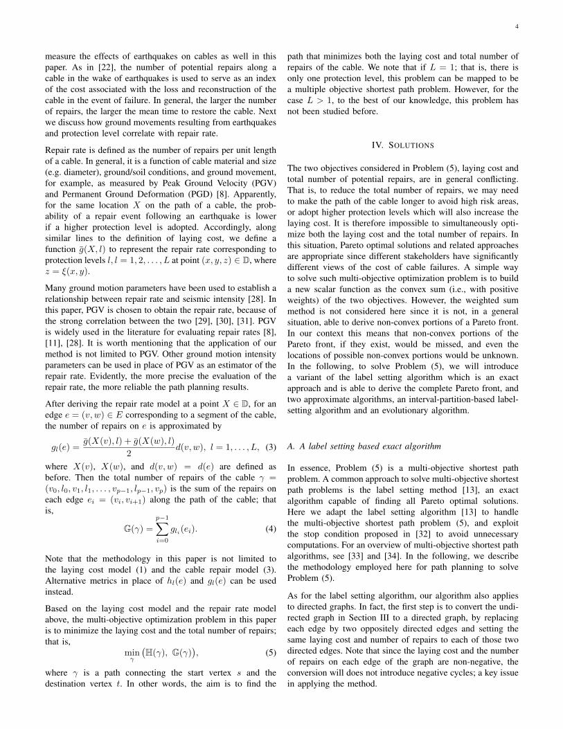
Here we use the simple example shown in Figure 1 to illustrateresults obtained by Algorithm 1. We will provide two morecomplex examples in the next section. Note that our objectiveis to find Pareto optimal paths from vertex 1 to vertex 7. Someof them are shown by Figure 2. The red lines in Figure 2 meanthe edges that adopt Level 2. On the other hand, black linesindicate edges with Level 1 without shielding protection. The

6

aggregated laying cost and total number of repairs of eachPareto optimal path are shown in Table I. From Figure 2 andTable I, we can observe the trade-off between the aggregatedlaying cost and aggregated total number of repairs. As canbe seen, lower total number of repairs means much moreinvestment in cable protection for the same path.

TABLE I: Results of the example shown by Figure 1.

a b c d eLaying cost 18 20 21 25 29

Repairs 32 29 24 18 15

vertices 1, 2, 5, 7 1, 2, 5, 7 1, 3, 5, 7 1, 3, 5, 7 1, 3, 5, 7

levels 1, 1, 1 1, 1, 2 1, 1, 1 2, 1, 2 2, 2, 2

1

2 4

3 5

6

7

(a) G = 32

1

2 4

3 5

6

7

(b) G = 29

1

2 4

3 5

6

7

(c) G = 24

1

2 4

3 5

6

7

(d) G = 18

1

2 4

3 5

6

7

(e) G = 15

Fig. 2: Selected Pareto optimal paths for the example shownin Figure 1.

Since multi-objective shortest path problems are known to beNP-hard [35], so is Problem (5). Following the analysis in [36],the computational complexity of Algorithm 1 can be derivedas

O(DLT 2K2 log(K)),

where D is the average graph degree, L is the total numberof available protection levels, T is the number of objectives(T = 2 in this paper), and K is the total number of non-dominated labels of all vertices. For an application with verylarge number of non-dominated labels, Algorithm 1 will becomputing-intensive. To accommodate this problem, we at-tempt and compare two approximation algorithms with limitedcomputational cost. These are described below.

B. An interval-partition-based approximate algorithm

In this paper, the interval-partition-based label-setting ap-proach (LS-IP) [37] which is a polynomial time approximationscheme with a performance guarantee is used to obtain theapproximate Pareto front. Given any fixed ε > 0, the algorithmcomputes, in a time that is polynomial in the input size and1ε , a (1 + ε)-Pareto curve Pε. A (1 + ε)-Pareto curve Pε is afinite set of feasible solutions such that each Pareto optimalsolution γ is within a factor of (1 + ε) of some γ′ ∈ Pε in allobjectives. The main idea of the algorithm is to partition thelabel sets as arrays of polynomial size in order to avoid keepall non-dominated solutions, while producing an approximate

Pareto set that can (1 + ε)-cover the Pareto optimal set. Moredetails of the algorithm can be refered to [37], [38].

We adapt the LS-IP in [38] to solve Problem (5) ap-proximately. To obtain a (1 + ε)-Pareto curve for agiven ε, the domain of the laying cost is partitioned intoblog

(1+ε)1n′nCmaxc+1 intervals [38], where Cmax is the ratio

of the maximum laying cost to the minimum laying cost onedges, n′ is the number of edges of the feasible path with mostedges and it is assumed to be equal to n−1 in [38], where n isthe number of vertices of the graph G. We note that, insteadof assuming n′ = n − 1, we can let n′ = n − 1, where nis the number of vertices on the non-dominated path γ withmaximal laying cost (or minimal total number of repairs) sinceany other non-dominated path has fewer number of verticesthan γ. This path γ can be derived by running Dijkstra’salgorithm before running the LS-IP. In some cases, as shownin Section V, n is much smaller than n, resulting in farfewer intervals being required, as well as reducing the runningtime of the algorithm and therefore saving computational costsignificantly. From [38], the computational complexity of theLS-IP is O(m(n log(nCmax)

ε )), where m is the number of edgesin the graph G.

C. An evolutionary algorithm

Evolutionary algorithms (EA) are a popular kind of heuristicsearch algorithm derived from the evolutionary process ofgenetic selection and variation. EAs use random and intel-ligent search to guide the search into the region of betterperformance in the search space. By the selection and vari-ation process, a new set of individuals is created at eachgeneration based on their fitness value. The breeding processborrowed from natural genetics make the evolution of popula-tions have better performance for the environment than theirpredecessors. In this paper, we adopt an improved methodbased on SPEA (Strength Pareto Evolutionary Algorithm),namely SPEA2 [39], [40], since it is reported to have betterperformance on approximating Pareto set for multi-objectiveoptimization problems comparing with other strategies. Mariaet al. [41] proposed a SPEA2 based evolutionary algorithmfor multi-objective shortest path problem.

We adapt the algorithm, namely EA-SPEA2, in [41] to con-sider multiple protection levels. Because there are multiplelevels for each edge, we randomly assign one of the protectionlevels to each initial path and offspring. More specifically, inthe initialization stage, we use a random walk to generate aset of initial paths P between the given two sources (s, t). Weassume that γ ∈ P is one of initial paths composed of j edges,i.e. e1, e2, ..., ej . A protection level is uniformly randomlyselected for each edge of γ. In the variation stage, there are twokinds of variation operators, path mutation and path crossover.For the path mutation, a randomly selected vertex v ∈ γ\{s, t}is mutated from path γ. After removing the vertex v andinserting a new auxiliary vertex v∗, a new path γ∗ is created.Suppose that in the path γ, the adjacent vertices of v are u1 andu2. For the new path γ∗, v∗ should be connected with nodes

7

u1 and u2 and the protection level of edge e(u1, v∗) and edge

e(v∗, u2) need to be assigned uniformly randomly. For thepath crossover operator, if a new path γ∗ is generated, only theconnecting edge of two predecessors needs to be reassigneda protection level. The running time and performance ofthe EA-SPEA2 heavily depends on the population size andmaximum number of generations. Using a larger populationand a bigger maximum number of generations may makethe generated non-dominated set approximate the Pareto frontmore accurate, and meanwhile will increase the computationalcost accordingly. For more details on the algorithm, the readercan refer to [39], [40], [41].

V. APPLICATIONS AND NUMERICAL RESULTS

In this section, we provide three applications to illustrate andcompare the three algorithms in Section IV. Firstly, in linewith our previous work [22], we apply Algorithm 1, LS-IP andEA-SPEA2 to a 2D landform scenario, where the PGV datais simulated by running the PSHA method. Then, we applythese three algorithms to two 3D landform scenarios based onearthquake hazard estimation data from USGS. Without lossof generality, we assume there are two protection levels forboth of these two scenarios. The aggregated laying cost andthe aggregated total number of repairs of different cables areestimated and (approximate) Pareto fronts are generated. Notethat the units of PGV and repair rate in this section are cm/sand number of repairs per km, respectively. We run the threealgorithms coded in Matlab R2014b on a Dell OPTIPLEX9020 computer (8 GB RAM, 3.6 GHz Intel(R) Core(TM) i7-4790 CPU).

A. Application to a 2D landform

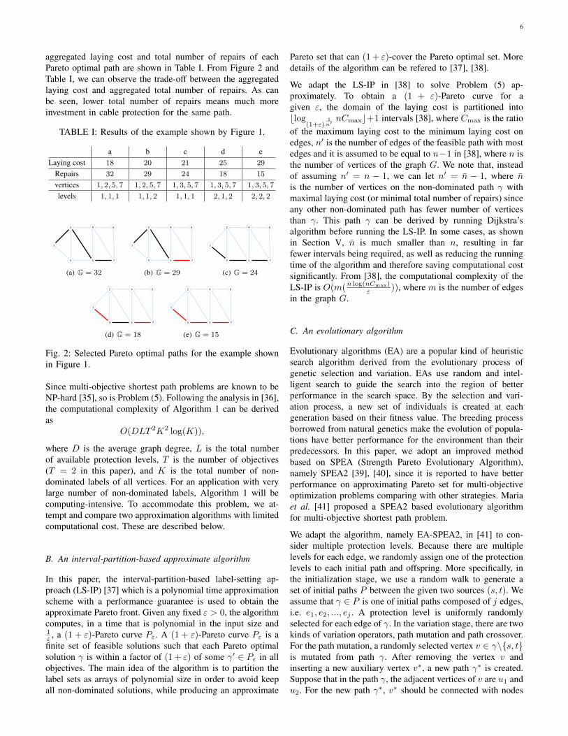
We apply the three algorithms to a 2D example on a planarregion as shown in Figure 3, where a 20 km long straightfault line, as a potential earthquake source, is assumed to belocated in the region. The coordinates of the two end sitesA and B of the fault line are [50 km, 40 km] and [50 km,60 km], respectively. According to the bounded-Gutenberg-Richter model [12], without loss of generality, we assumeearthquakes of magnitude from mmin = 5 to mmax = 6.5are generated by this earthquake fault line source. Using thePGV data produced in our previous work, [22], and shown inFigure 3, we calculated the corresponding repair rate for eachsite (x, y). Assuming there are two protection levels, Level 1(low level) and Level 2 (high level), we calculate repair ratesby the following equations.

g1(x, y) = e1.30×lnvx,y−7.21, (6a)

g2(x, y) =e1.30×lnvx,y−7.21

4.95, (6b)

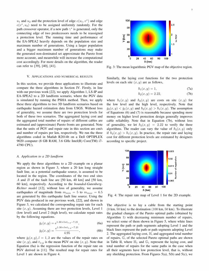
where gl(x, y), l = 1, 2 are the values of the repair rates onsite (x, y), and vx,y is the mean PGV on site (x, y). Note thatEquation (6a) is the regression function of the repair rate onPGV derived in [11]. The resulted map for repair rates forLevel 1 are shown in Figure 4.

Fig. 3: The mean logarithmic PGV map of the objective region.

Similarly, the laying cost functions for the two protectionlevels on each site (x, y) are as follows,

~1(x, y) = 1, (7a)~2(x, y) = 2.22, (7b)

where ~1(x, y) and ~2(x, y) are costs on site (x, y) forthe low level and the high level, respectively. Note thatg2(x, y) < g1(x, y) and ~2(x, y) > ~1(x, y). The assumptionof Equations (6) and (7) is reasonable because spending moremoney on higher level protection design generally improvescable reliability. Note that in Equation (7b), without lossof generality, we let ~2(x, y) = 2.22 to verify the threealgorithms. The reader can vary the value of ~2(x, y) onlyif ~2(x, y) > ~1(x, y). In practice, the repair rate and layingcost for different protection levels are estimated by designersaccording to specific project.

Fig. 4: The repair rate map of Level 1 for the 2D example.

The objective is to lay a cable from the starting point(0 km, 50 km) to the destination (100 km, 50 km). To illustratethe gradual changes of the Pareto optimal paths (obtained byAlgorithm 1) with decreasing minimum number of repairs,we select some of them shown in Figure 5, where white linesrepresent the path or path segments adopting Level 1 and theblack lines represent the path or path segments adopting Level2. The aggregated laying cost, H, and aggregated total numberof repairs, G, of the selected Pareto optimal paths are shownin Table II, where H1 and G1 represent the laying cost, andtotal number of repairs for the same paths in the case whenall their segments have low protection level, that is, withoutany shielding protection. From Figures 5(a), 5(b) and 5(c), we

8

can see that initially, providing protection for some parts ofthe cable in the high PGV region can significantly decreasethe total number of repairs. As the total number of repairsdecreases the optimal paths will avoid the high PGV region todecrease repairs though their length increases. Notice, for thedifferent optimal paths, the alternative ways of reducing risk(reducing the number of repairs) by either adding segmentswith protection as the black lines in Figures 5(c) and 5(e)indicate, or by increasing the length of the cable and avoidingthe high risk areas as shown in Figures 5(d) and 5(f). FromTable II and Figure 5, we observe the trade-off between theaggregated laying cost and aggregated total number of repairs;that is, the smaller the total number of repairs, the greater isthe laying cost.

TABLE II: Aggregated laying cost and total number of repairsof selected Pareto optimal paths (obtained by Algorithm 1) inthe 2D example.

H(γ∗) G(γ∗) H1(γ∗) G1(γ∗)

a 100.0000 1.0648 100.0000 1.0648

b 106.1199 0.9667 100.0000 1.0648

c 112.2398 0.8767 100.0000 1.0648

d 114.0833 0.8506 114.0833 0.8506

e 114.6878 0.8435 100.0000 1.0648

f 118.2254 0.7820 118.2254 0.7820

g 123.1960 0.7305 123.1960 0.7305

h 123.5915 0.7303 122.3675 0.7370

i 125.6812 0.7159 125.6812 0.7159

j 125.7036 0.7126 100.0000 1.0648

k 126.8679 0.7112 123.1960 0.7305

l 137.9434 0.5970 100.0000 1.0648

m 164.8709 0.4198 100.0000 1.0648

n 222.3980 0.2153 100.0000 1.0648

o 259.2461 0.1631 116.5685 0.8067

p 335.4937 0.1299 150.8528 0.6424

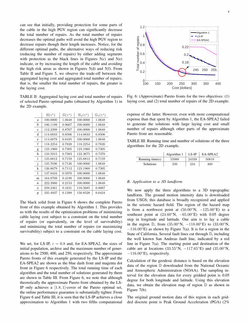
The black solid front in Figure 6 shows the complete Paretofront of this example obtained by Algorithm 1. This providesus with the results of the optimization problems of minimizingcable laying cost subject to a constraint on the total numberof repairs (or equivalently, on the level of survivability)and minimizing the total number of repairs (or maximizingsurvivability) subject to a constraint on the cable laying cost.

We set, for LS-IP, ε = 0.8 and, for EA-SPEA2, the sizes ofinitial population, archive and the maximum number of gener-ations to be 2500, 400, and 250, respectively. The approximatePareto fronts of this example generated by the LS-IP and theEA-SPEA2 are shown as the blue dash front and magenta dotfront in Figure 6 respectively. The total running time of eachalgorithm and the total number of solutions generated by themare shown in Table III. From Figure 6, we note that althoughtheoretically the approximate Pareto front obtained by the LS-IP only achieves a [1.8, 1]-cover of the Pareto optimal set,the online performance guarantee is substantially tighter. FromFigure 6 and Table III, it is seen that the LS-IP achieves a closeapproximation to Algorithm 1 with two fifths computational

Cost [dollars]100 150 200 250 300 350 400

Tot

al n

umbe

r of

rep

airs

0

0.2

0.4

0.6

0.8

1

1.2

Algorithm 1

LS-IP

EA-SPEA2

245 250 255

0.18

0.2

0.22

Fig. 6: (Approximate) Pareto fronts for the two objectives: (1)laying cost, and (2) total number of repairs of the 2D example.

expense of the latter. However, even with more computationalexpense than that spent by Algorithm 1, the EA-SPEA2 failedto generate the solutions with large laying cost and smallnumber of repairs although other parts of the approximatePareto front are reasonable.

TABLE III: Running time and number of solutions of the threealgorithms for the 2D example.

Algorithm 1 LS-IP EA-SPEA2Running time(s) 55988 24339 50818

Solutions 339 234 400

B. Application to a 3D landform

We now apply the three algorithms to a 3D topographiclandform. The ground motion intensity data is downloadedfrom USGS; this database is broadly recognized and appliedin the seismic hazard field. The region of the hazard mapis from a northwest point at (50.00◦N, −125.00◦E) to asoutheast point at (24.60◦N, −65.00◦E) with 0.05 degreestep in longitude and latitude. Our aim is to lay a cablein the region D, from (35.00◦N, −118.00◦E) to (33.00◦N,−116.00◦E) as shown by Figure 7(a). It is for a region in theState of California. Several fault lines cut through D, includingthe well known San Andreas fault line, indicated by a redline in Figure 7(a). The starting point and destination of thecable are at locations (33.55◦N, −117.65◦E) and (35.00◦N,−116.00◦E), respectively.

Calculation of the geodesic distance is based on the elevationdata of the region D downloaded from the National Oceanicand Atmospheric Administration (NOAA). The sampling in-terval for the elevation data for every gridded point is 0.05degree for both longitude and latitude. Using this elevationdata, we obtain the elevation map of region D as shown inFigure 7(b).

The original ground motion data of this region in each grid-ded discrete point is Peak Ground Acceleration (PGA) (2%

9

(a) (b) (c) (d)

(e) (f) (g) (h)

(i) (j) (k) (l)

(m) (n) (o) (p)

Fig. 5: Selected Pareto optimal paths (obtained by Algorithm 1) in the 2D example. The white lines represent the path orpath segments adopting low protection level (Level 1) and the black lines represent the path or path segments adopting highprotection level (Level 2).

(a) Region D. Source: GoogleEarth.

(b) Elevation map of D. Source:NOAA.

Fig. 7: Geography of Region D.

probability of exceedance in 50 years, Vs30 = 760 m/s). Oneof our objective is to calculate total number of repairs of thedesigned path, which requires conversion of PGA to PGV. Weuse the transform equation from Wald [42] as follows,

log10(v) = 1.0548 · log10(PGA)− 1.5566, (8)

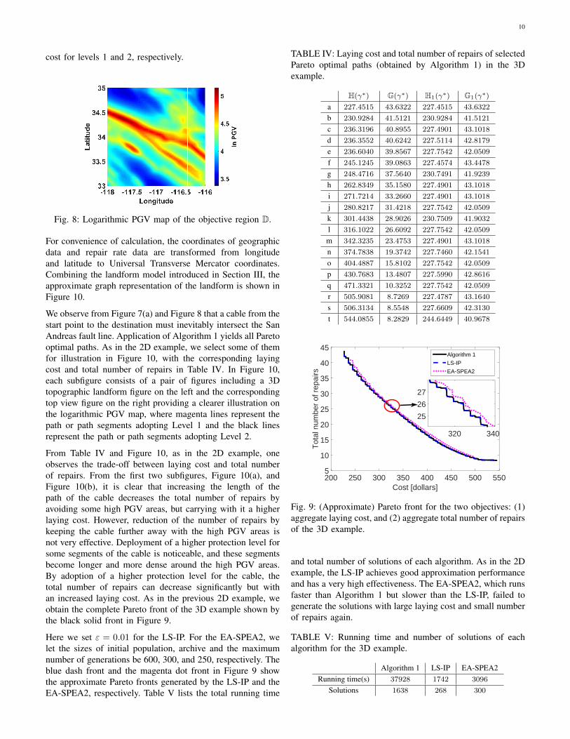
where v is PGV. The shaded PGV map of the region D isgiven in Figure 8. In this example, we also assume there aretwo protection levels, low level (Level 1) and high level (Level2). The PGV data is used to calculate the corresponding valuesof the repair rate of each gridded point for the two protectionlevels using Equations (6a) and (6b). We use the same layingcost functions, Equations (7a) and (7b), to calculate the laying

10

cost for levels 1 and 2, respectively.

Fig. 8: Logarithmic PGV map of the objective region D.

For convenience of calculation, the coordinates of geographicdata and repair rate data are transformed from longitudeand latitude to Universal Transverse Mercator coordinates.Combining the landform model introduced in Section III, theapproximate graph representation of the landform is shown inFigure 10.

We observe from Figure 7(a) and Figure 8 that a cable from thestart point to the destination must inevitably intersect the SanAndreas fault line. Application of Algorithm 1 yields all Paretooptimal paths. As in the 2D example, we select some of themfor illustration in Figure 10, with the corresponding layingcost and total number of repairs in Table IV. In Figure 10,each subfigure consists of a pair of figures including a 3Dtopographic landform figure on the left and the correspondingtop view figure on the right providing a clearer illustration onthe logarithmic PGV map, where magenta lines represent thepath or path segments adopting Level 1 and the black linesrepresent the path or path segments adopting Level 2.

From Table IV and Figure 10, as in the 2D example, oneobserves the trade-off between laying cost and total numberof repairs. From the first two subfigures, Figure 10(a), andFigure 10(b), it is clear that increasing the length of thepath of the cable decreases the total number of repairs byavoiding some high PGV areas, but carrying with it a higherlaying cost. However, reduction of the number of repairs bykeeping the cable further away with the high PGV areas isnot very effective. Deployment of a higher protection level forsome segments of the cable is noticeable, and these segmentsbecome longer and more dense around the high PGV areas.By adoption of a higher protection level for the cable, thetotal number of repairs can decrease significantly but withan increased laying cost. As in the previous 2D example, weobtain the complete Pareto front of the 3D example shown bythe black solid front in Figure 9.

Here we set ε = 0.01 for the LS-IP. For the EA-SPEA2, welet the sizes of initial population, archive and the maximumnumber of generations be 600, 300, and 250, respectively. Theblue dash front and the magenta dot front in Figure 9 showthe approximate Pareto fronts generated by the LS-IP and theEA-SPEA2, respectively. Table V lists the total running time

TABLE IV: Laying cost and total number of repairs of selectedPareto optimal paths (obtained by Algorithm 1) in the 3Dexample.

H(γ∗) G(γ∗) H1(γ∗) G1(γ∗)

a 227.4515 43.6322 227.4515 43.6322

b 230.9284 41.5121 230.9284 41.5121

c 236.3196 40.8955 227.4901 43.1018

d 236.3552 40.6242 227.5114 42.8179

e 236.6040 39.8567 227.7542 42.0509

f 245.1245 39.0863 227.4574 43.4478

g 248.4716 37.5640 230.7491 41.9239

h 262.8349 35.1580 227.4901 43.1018

i 271.7214 33.2660 227.4901 43.1018

j 280.8217 31.4218 227.7542 42.0509

k 301.4438 28.9026 230.7509 41.9032

l 316.1022 26.6092 227.7542 42.0509

m 342.3235 23.4753 227.4901 43.1018

n 374.7838 19.3742 227.7460 42.1541

o 404.4887 15.8102 227.7542 42.0509

p 430.7683 13.4807 227.5990 42.8616

q 471.3321 10.3252 227.7542 42.0509

r 505.9081 8.7269 227.4787 43.1640

s 506.3134 8.5548 227.6609 42.3130

t 544.0855 8.2829 244.6449 40.9678

Cost [dollars]200 250 300 350 400 450 500 550

Tot

al n

umbe

r of

rep

airs

5

10

15

20

25

30

35

40

45

320 340

25

26

27

Algorithm 1

LS-IP

EA-SPEA2

Fig. 9: (Approximate) Pareto front for the two objectives: (1)aggregate laying cost, and (2) aggregate total number of repairsof the 3D example.

and total number of solutions of each algorithm. As in the 2Dexample, the LS-IP achieves good approximation performanceand has a very high effectiveness. The EA-SPEA2, which runsfaster than Algorithm 1 but slower than the LS-IP, failed togenerate the solutions with large laying cost and small numberof repairs again.

TABLE V: Running time and number of solutions of eachalgorithm for the 3D example.

Algorithm 1 LS-IP EA-SPEA2Running time(s) 37928 1742 3096

Solutions 1638 268 300

11

(a) (b)

(c) (d)

(e) (f)

(g) (h)

(i) (j)

12

(k) (l)

(m) (n)

(o) (p)

(q) (r)

(s) (t)

Fig. 10: Selected Pareto optimal paths (obtained by Algorithm 1) in the 3D example. The magenta lines represent the path orpath segments adopting low protection level (Level 1) and the black lines represent the path or path segments adopting highprotection level (Level 2).

13

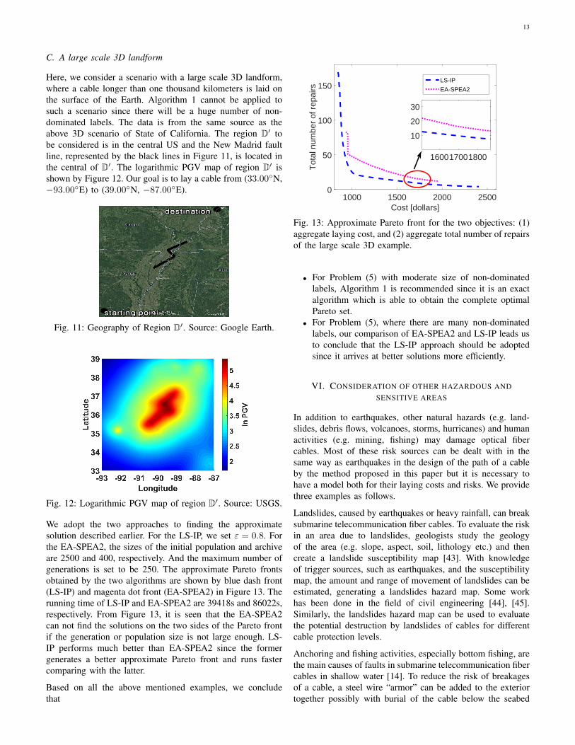
C. A large scale 3D landform

Here, we consider a scenario with a large scale 3D landform,where a cable longer than one thousand kilometers is laid onthe surface of the Earth. Algorithm 1 cannot be applied tosuch a scenario since there will be a huge number of non-dominated labels. The data is from the same source as theabove 3D scenario of State of California. The region D′ tobe considered is in the central US and the New Madrid faultline, represented by the black lines in Figure 11, is located inthe central of D′. The logarithmic PGV map of region D′ isshown by Figure 12. Our goal is to lay a cable from (33.00◦N,−93.00◦E) to (39.00◦N, −87.00◦E).

Fig. 11: Geography of Region D′. Source: Google Earth.

Fig. 12: Logarithmic PGV map of region D′. Source: USGS.

We adopt the two approaches to finding the approximatesolution described earlier. For the LS-IP, we set ε = 0.8. Forthe EA-SPEA2, the sizes of the initial population and archiveare 2500 and 400, respectively. And the maximum number ofgenerations is set to be 250. The approximate Pareto frontsobtained by the two algorithms are shown by blue dash front(LS-IP) and magenta dot front (EA-SPEA2) in Figure 13. Therunning time of LS-IP and EA-SPEA2 are 39418s and 86022s,respectively. From Figure 13, it is seen that the EA-SPEA2can not find the solutions on the two sides of the Pareto frontif the generation or population size is not large enough. LS-IP performs much better than EA-SPEA2 since the formergenerates a better approximate Pareto front and runs fastercomparing with the latter.

Based on all the above mentioned examples, we concludethat

Cost [dollars]1000 1500 2000 2500

Tot

al n

umbe

r of

rep

airs

0

50

100

150

160017001800

10

20

30

LS-IP

EA-SPEA2

Fig. 13: Approximate Pareto front for the two objectives: (1)aggregate laying cost, and (2) aggregate total number of repairsof the large scale 3D example.

• For Problem (5) with moderate size of non-dominatedlabels, Algorithm 1 is recommended since it is an exactalgorithm which is able to obtain the complete optimalPareto set.

• For Problem (5), where there are many non-dominatedlabels, our comparison of EA-SPEA2 and LS-IP leads usto conclude that the LS-IP approach should be adoptedsince it arrives at better solutions more efficiently.

VI. CONSIDERATION OF OTHER HAZARDOUS ANDSENSITIVE AREAS

In addition to earthquakes, other natural hazards (e.g. land-slides, debris flows, volcanoes, storms, hurricanes) and humanactivities (e.g. mining, fishing) may damage optical fibercables. Most of these risk sources can be dealt with in thesame way as earthquakes in the design of the path of a cableby the method proposed in this paper but it is necessary tohave a model both for their laying costs and risks. We providethree examples as follows.

Landslides, caused by earthquakes or heavy rainfall, can breaksubmarine telecommunication fiber cables. To evaluate the riskin an area due to landslides, geologists study the geologyof the area (e.g. slope, aspect, soil, lithology etc.) and thencreate a landslide susceptibility map [43]. With knowledgeof trigger sources, such as earthquakes, and the susceptibilitymap, the amount and range of movement of landslides can beestimated, generating a landslides hazard map. Some workhas been done in the field of civil engineering [44], [45].Similarly, the landslides hazard map can be used to evaluatethe potential destruction by landslides of cables for differentcable protection levels.

Anchoring and fishing activities, especially bottom fishing, arethe main causes of faults in submarine telecommunication fibercables in shallow water [14]. To reduce the risk of breakagesof a cable, a steel wire “armor” can be added to the exteriortogether possibly with burial of the cable below the seabed

14

if the cable passes through anchorage and fishery areas or,alternatively, the route of the cable can avoid such areas. Tosolve the problem of path planning and the non-homogenousconstruction of the cable taking into account such areas, weconsider several protection levels; for example, lightweightcable (Level 1), single armored cable (Level 2), and doublearmored cable (Level 3). The laying cost of the cable at eachlocation for the protection levels can be estimated from theprice of each type of the cable, and the cost of labor andequipment. Also, for each protection level, the cable repairrate can be estimated from historical data of fishing activitiesand analyses of the mechanism of cable damage by fishingactivities.

For areas that have to be avoided by the cable, such as areasthose of high ecological value, or which are rocky or havemilitary utility, the laying cost of each site in these areas canbe set to be infinity.

VII. CONCLUSION

We have considered the path optimization and non-homogenous construction problem for a telecommunicationcable connecting two points in high risk areas when multipleprotection levels are available. Regarding laying cost and totalnumber of repairs of the cable as the two objectives, wehave formulated the problem as a multi-objective shortest pathproblem. We have modeled the Earth surface as a graph of TINand evaluated the repair rate using ground motion intensitymeasures of earthquake events. The multi-objective shortestpath problem has been solved using the label setting algorithmto obtain the Pareto front for the two objectives via numerouscomputer experiments. The Pareto front enables us to solve thefollowing two single objective optimization problems.

1) Find the least-laying-cost cable and corresponding pro-tection level for each segment of the cable subject to aconstraint on the total number of repairs;

2) Find the cable with minimum total number of repairsand the protection level for each segment subject to aconstraint on the total budget.

For the problem with a large number of non-dominatedlabels, the interval-partition-based label-setting algorithm canbe used to obtain an approximate Pareto front in a reasonablerunning time. In future work, we will investigate algorithmsthat achieve good approximations more efficiently for largeproblems.

REFERENCES

[1] TeleGeography, “Submarine cable map,” 2016 (accessed onMay 31, 2017). [Online]. Available: https://www.telegeography.com/telecom-maps/submarine-cable-map/index.html

[2] Submarine Telecoms Forum, “Submarine telecoms industry report,”2015 (accessed on May 31, 2017). [Online]. Available: http://www.subtelforum.com/Report4/

[3] W. Qiu, “Submarine cables cut after Taiwan earthquake in Dec2006,” Mar. 2011 (accessed on May 31, 2017). [Online]. Available:http://www.submarinenetworks.com

[4] mi2g, “More than 1% GDP drop estimated per week of Internetblackout,” Jul. 2005 (accessed on May 31, 2017). [Online]. Available:http://www.mi2g.com

[5] T. P. Dubendorfer, “Impact analysis, early detection and mitigation oflarge-scale Internet attacks,” Ph.D. dissertation, Swiss Federal Instituteof Technology Zurich, 2005.

[6] A. Markow, “Summary of undersea fiber optic net-work technology and systems,” accessed on May 31,2017. [Online]. Available: http://hmorell.com/sub cable/documents/BasicsofSubmarineSystemInstallationandOperation.pdf

[7] E. Tahchi, private communication, Oct. 2016.

[8] American Lifeline Alliance, “Seismic fragility formulations for watersystems, Part I-Guideline,” 2001 (accessed on May 31, 2017). [Online].Available: http://www.americanlifelinesalliance.org

[9] Y. Wang and T. D. O’Rourke, Seismic performance evaluation of watersupply systems. Buffalo, New York, USA: Multidisciplinary Center forEarthquake Engineering Research, 2008.

[10] M. Fragiadakis and S. E. Christodoulou, “Seismic reliability assessmentof urban water networks,” Earthquake Engineering & Structural Dy-namics, vol. 43, no. 3, pp. 357–374, Aug. 2014.

[11] S.-S. Jeon and T. D. O’Rourke, “Northridge earthquake effects onpipelines and residential buildings,” Bulletin of the Seismological Societyof America, vol. 95, no. 1, pp. 294–318, Feb. 2005.

[12] J. Baker, “An introduction to probabilistic seismic hazard analysis,”Stanford University, White Paper. Version 2.0, 2013 (accessed on May31, 2017). [Online]. Available: https://scits.stanford.edu/sites/default/files/baker 2013 intro psha v2.pdf

[13] E. Q. V. Martins, “On a multicriteria shortest path problem,” EuropeanJournal of Operational Research, vol. 16, no. 2, pp. 236–245, May 1984.

[14] D. R. Burnett, R. Beckman, and T. M. Davenport, Submarine Cables:the handbook of Law and Policy. Leiden, Netherlands: Martinus NijhoffPublishers, 2013.

[15] D. L. Msongaleli, F. Dikbiyik, M. Zukerman, and B. Mukherjee,“Disaster-aware submarine fiber-optic cable deployment for mesh net-works,” IEEE/OSA Journal of Lightwave Technology, vol. 34, no. 18,pp. 4293–4303, Jul. 2016.

[16] M. Zhao, T. W. S. Chow, P. Tang, Z. Wang, J. Guo, and M. Zukerman,“Route selection for cabling considering cost minimization and earth-quake survivability via a semi-supervised probabilistic model,” IEEETransactions on Industrial Informatics, vol. 13, no. 2, pp. 502–511, Apr.2017.

[17] C. Cao, M. Zukerman, W. Wu, J. H. Manton, and B. Moran, “Sur-vivable topology design of submarine networks,” IEEE/OSA Journal ofLightwave Technology, vol. 31, no. 5, pp. 715–730, Mar. 2013.

[18] C. Cao, Z. Wang, M. Zukerman, J. Manton, A. Bensoussan, andY. Wang, “Optimal cable laying across an earthquake fault line con-sidering elliptical failures,” IEEE Transactions on Reliability, vol. 65,no. 3, pp. 1536–1550, Sept. 2016.

[19] P. N. Tran and H. Saito, “Geographical route design of physical networksusing earthquake risk information,” IEEE Communications Magazine,vol. 54, no. 7, pp. 131–137, Jul. 2016.

[20] ——, “Enhancing physical network robustness against earthquake disas-ters with additional links,” IEEE/OSA Journal of Lightwave Technology,vol. 34, no. 22, pp. 5226–5238, Nov. 2016.

[21] H. Saito, “Geometric evaluation of survivability of disaster-affectednetwork with probabilistic failure,” in Proceedings of the 33rd AnnualIEEE International Conference on Computer Communications, Toronto,Canada, 2014, pp. 1608–1616.

15

[22] Z. Wang, Q. Wang, M. Zukerman, J. Guo, Y. Wang, G. Wang, J. Yang,and B. Moran, “Multiobjective path optimization for critical infras-tructure links with consideration to seismic resilience,” To appear inComputer-Aided Civil and Infrastructure Engineering, 2017.

[23] J. Zhang, E. Modiano, and D. Hay, “Enhancing network robustnessvia shielding,” in Proceedings of 11th International Conference on theDesign of Reliable Communication Networks, Kansas, USA, 2015, pp.17–24.

[24] ——, “Enhancing network robustness via shielding,” IEEE/ACMTransactions on Networking, 2017. [Online]. Available: http://dx.doi.org/10.1109/TNET.2017.2689019

[25] D. Greenspan, Introduction to partial differential equations. Mineola,New York, USA: Dover Publications, INC., 2000.

[26] T. K. Peucker, R. J. Fowler, J. J. Little, and D. M. Mark, “Thetriangulated irregular network,” in Proceedings of the DTM Symposium,St. Louis, Missouri, USA, 1978, pp. 24–31.

[27] J. Lee, “Comparison of existing methods for building triangular irregularnetwork, models of terrain from grid digital elevation models,” Interna-tional Journal of Geographical Information System, vol. 5, no. 3, pp.267–285, 1991.

[28] O. Pineda-Porras and M. Najafi, “Seismic damage estimation for buriedpipelines: Challenges after three decades of progress,” Journal ofPipeline Systems Engineering and Practice, vol. 1, no. 1, pp. 19–24,Jan. 2010.

[29] T. D. O’Rourke, S. Toprak, and Y. Sano, “Factors affecting water supplydamage caused by the Northridge earthquake,” in Proceedings of the 6thUS National Conference on Earthquake Engineering, Seattle, WA, USA,1998, pp. 1–12.

[30] S. Toprak, “Earthquake effects on buried lifeline systems,” Ph.D. dis-sertation, Cornell University, 1998.

[31] S. Toprak and F. Taskin, “Estimation of earthquake damage to buriedpipelines caused by ground shaking,” Natural hazards, vol. 40, no. 1,pp. 1–24, Sept. 2007.

[32] S. Demeyer, J. Goedgebeur, P. Audenaert, M. Pickavet, and P. De-meester, “Speeding up Martins’ algorithm for multiple objective shortestpath problems,” 4OR-Q J Oper Res, vol. 11, no. 4, pp. 323–348, Feb.2013.

[33] A. Raith and M. Ehrgott, “A comparison of solution strategies forbiobjective shortest path problems,” Computers & Operations Research,vol. 36, no. 4, pp. 1299–1331, Apr. 2009.

[34] J. C. Clımaco and M. Pascoal, “Multicriteria path and tree problems:discussion on exact algorithms and applications,” International Trans-actions in Operational Research, vol. 19, no. 1-2, pp. 63–98, Jan. 2012.

[35] M. R. Gary and D. S. Johnson, Computers and Intractability: A Guideto the Theory of NP-completeness. New York, USA: WH Freeman andCompany, 1979.

[36] R. G. Garroppo, S. Giordano, and L. Tavanti, “A survey on multi-constrained optimal path computation: Exact and approximate algo-rithms,” Computer Networks, vol. 54, no. 17, pp. 3081–3107, Dec. 2010.

[37] S. Vassilvitskii and M. Yannakakis, “Efficiently computing succincttrade-off curves,” Theoretical Computer Science, vol. 348, no. 2-3, pp.334–356, Dec. 2005.

[38] G. Tsaggouris and C. Zaroliagis, “Multiobjective optimization: ImprovedFPTAS for shortest paths and non-linear objectives with applications,”Theory of Computing Systems, vol. 45, no. 1, pp. 162–186, Jun. 2009.

[39] E. Zitzler and L. Thiele, “Multiobjective evolutionary algorithms: a com-parative case study and the strength Pareto approach,” IEEE Transactionson Evolutionary Computation, vol. 3, no. 4, pp. 257–271, Nov. 1999.

[40] E. Zitzler, M. Laumanns, and L. Thiele, “SPEA2: Improving the strengthPareto evolutionary algorithm,” Swiss Federal Institute of Technology(ETH) Zurich, Tech. Rep. TIK-Report 103, 2001 (accessed on May 31,2017). [Online]. Available: http://e-collection.library.ethz.ch/eserv/eth:24689/eth-24689-01.pdf

[41] J. Maria, A. Pangilinan, and G. K. Janssens, “Evolutionary algorithmsfor the multiobjective shortest path problem,” International Journalof Mathematical, Computational, Physical, Electrical and ComputerEngineering, vol. 1, no. 1, pp. 7–12, Jan. 2007.

[42] D. J. Wald, “Relationships between peak ground acceleration, peakground velocity, and modified Mercalli intensity in California,” Earth-quake Spectra, vol. 15, no. 3, pp. 557–564, Aug. 1999.

[43] H. Shahabi and M. Hashim, “Landslide susceptibility mapping usingGIS-based statistical models and Remote sensing data in tropical envi-ronment,” Scientific reports, vol. 5, pp. 1–15, Apr. 2015.

[44] R. L. Baum, D. L. Galloway, and E. L. Harp, “Landslide andland subsidence hazards to pipelines,” Geological Survey (US),Tech. Rep., 2008 (accessed on May 31, 2017). [Online]. Available:https://pubs.usgs.gov/of/2008/1164/pdf/OF08-1164 508.pdf

[45] D. G. Honegger, J. D. Hart, R. Phillips, C. Popelar, and R. W.Gailing, “Recent PRCI guidelines for pipelines exposed to landslideand ground subsidence hazards,” in Proceedings of 8th InternationalPipeline Conference, Calgary, Alberta, Canada, 2010, pp. 71–80.