a search for astrophysical neutrino point sources with
TRANSCRIPT
A Search for Astrophysical Neutrino Point Sources with
Super-Kamiokande
Eric Thrane
A dissertation submitted in partial fulfillment ofthe requirements for the degree of
Doctor of Philosophy
University of Washington
2008
Program Authorized to Offer Degree: Physics

University of WashingtonGraduate School
This is to certify that I have examined this copy of a doctoral dissertation by
Eric Thrane
and have found that it is complete and satisfactory in all respects,and that any and all revisions required by the final
examining committee have been made.
Chair of the Supervisory Committee:
R. Jeffrey Wilkes
Reading Committee:
R. Jeffrey Wilkes
Thompson Burnett
Alec Habig
Jens Gundlach
Date:

In presenting this dissertation in partial fulfillment of the requirements for the doctoraldegree at the University of Washington, I agree that the Library shall make its copiesfreely available for inspection. I further agree that extensive copying of this dissertation isallowable only for scholarly purposes, consistent with “fair use” as prescribed in the U.S.Copyright Law. Requests for copying or reproduction of this dissertation may be referredto Proquest Information and Learning, 300 North Zeeb Road, Ann Arbor, MI 48106-1346,1-800-521-0600, to whom the author has granted “the right to reproduce and sell (a) copiesof the manuscript in microform and/or (b) printed copies of the manuscript made frommicroform.”
Signature
Date

University of Washington
Abstract
A Search for Astrophysical Neutrino Point Sources with Super-Kamiokande
Eric Thrane
Chair of the Supervisory Committee:Professor R. Jeffrey Wilkes
Department of Physics
The observation of cosmic rays with energies in excess of 1018 eV has helped spawn the
burgeoning field of ultra-high-energy (UHE) astronomy. A major effort is now underway
to determine how and where these particles are created. Models range from conventional
mechanisms such as “cosmic accelerators,” in which protons are accelerated by electromag-
netic fields, to exotic models positing the decay of hypothetical super-heavy particles. It is
thought that the mechanism responsible for UHE cosmic rays may also create copious high-
energy neutrinos (> 1GeV) with fluxes which may be within the reach of existing or planned
experiments. These sources are referred to as “point sources” to distinguish them from other
nearby sources such as atmospheric neutrinos, which—originating in Earth’s atmosphere—
do not exhibit the pointlike spatial clustering that characterizes a distant astrophysical
signal. Since neutrinos carry no charge, their paths are not obscured by magnetic fields like
protons, and so they offer a unique window into the UHE universe. In this thesis we aim to
develop a maximally efficient algorithm for measuring the flux from neutrino point sources.
The algorithm is applied to the upward-going muon dataset at Super-Kamiokande. We find
interesting signals from two sources: RX J1713.7-3946 (97.5-99.8% CL) and GRB 991004B
(95.3% CL). We set limits on the flux of neutrinos from a variety of suspected point sources
and for every point in the sky below dec < +54.

TABLE OF CONTENTS
Page
List of Figures . . . . . . . . . . . . . . . . . . . . . . . . . . . . . . . . . . . . . . . . iv
List of Tables . . . . . . . . . . . . . . . . . . . . . . . . . . . . . . . . . . . . . . . . . xi
Glossary . . . . . . . . . . . . . . . . . . . . . . . . . . . . . . . . . . . . . . . . . . . . xiv
Chapter 1: Theoretical Motivation for Neutrino Point Sources . . . . . . . . . . . 1
1.1 Definition and Overview . . . . . . . . . . . . . . . . . . . . . . . . . . . . . . 1
1.2 Current Trends in Neutrino Astronomy . . . . . . . . . . . . . . . . . . . . . 2
1.3 An Introduction to UHE Cosmic Rays . . . . . . . . . . . . . . . . . . . . . . 3
1.4 Cosmic Rays and Neutrinos: The Waxman-Bahcall Limit . . . . . . . . . . . 9
1.5 Top-Down Versus Bottom-Up . . . . . . . . . . . . . . . . . . . . . . . . . . . 10
1.6 Modeling Cosmic Accelerators . . . . . . . . . . . . . . . . . . . . . . . . . . . 11
1.7 Scenarios for Cosmic Acceleration . . . . . . . . . . . . . . . . . . . . . . . . . 18
1.8 Related Searches and Experiments . . . . . . . . . . . . . . . . . . . . . . . . 29
Chapter 2: Atmospheric Neutrinos and the Earth Shadow Effect . . . . . . . . . . 33
2.1 From Cosmic Rays to Atmospheric Neutrinos . . . . . . . . . . . . . . . . . . 33
2.2 Bartol and Honda Fluxes . . . . . . . . . . . . . . . . . . . . . . . . . . . . . 37
2.3 Oscillations . . . . . . . . . . . . . . . . . . . . . . . . . . . . . . . . . . . . . 38
2.4 Neutrino-Nucleon Scattering and the Earth Shadow . . . . . . . . . . . . . . 40
Chapter 3: The Super-Kamiokande Detector . . . . . . . . . . . . . . . . . . . . . 44
3.1 Cherenkov Radiation . . . . . . . . . . . . . . . . . . . . . . . . . . . . . . . . 44
3.2 Site . . . . . . . . . . . . . . . . . . . . . . . . . . . . . . . . . . . . . . . . . 50
3.3 Detector . . . . . . . . . . . . . . . . . . . . . . . . . . . . . . . . . . . . . . . 51
3.4 Data Acquisition . . . . . . . . . . . . . . . . . . . . . . . . . . . . . . . . . . 55
3.5 Trigger System . . . . . . . . . . . . . . . . . . . . . . . . . . . . . . . . . . . 59
3.6 Additional Detector Systems . . . . . . . . . . . . . . . . . . . . . . . . . . . 60
3.7 Water Transparency Calibration . . . . . . . . . . . . . . . . . . . . . . . . . 63
i
3.8 Additional Calibration Procedures . . . . . . . . . . . . . . . . . . . . . . . . 68
3.9 The Super-Kamiokande Accident and Subsequent Phases of Operation . . . . 75
Chapter 4: Monte Carlo Simulations . . . . . . . . . . . . . . . . . . . . . . . . . . 78
4.1 Overview . . . . . . . . . . . . . . . . . . . . . . . . . . . . . . . . . . . . . . 78
4.2 Atmospheric Neutrino MC with NEUT . . . . . . . . . . . . . . . . . . . . . . . 79
4.3 Point Source Monte Carlo . . . . . . . . . . . . . . . . . . . . . . . . . . . . . 81
4.4 skdetsim . . . . . . . . . . . . . . . . . . . . . . . . . . . . . . . . . . . . . . 84
Chapter 5: Upward-Going Muon Data Reduction . . . . . . . . . . . . . . . . . . 87
5.1 Upward-Going Muons . . . . . . . . . . . . . . . . . . . . . . . . . . . . . . . 87
5.2 Overview of the Upmu Reduction . . . . . . . . . . . . . . . . . . . . . . . . . 90
5.3 umred1st: The First Reduction . . . . . . . . . . . . . . . . . . . . . . . . . . 91
5.4 umred2nd: The Second Reduction . . . . . . . . . . . . . . . . . . . . . . . . 93
5.5 umred3rd: The Third Reduction . . . . . . . . . . . . . . . . . . . . . . . . . 97
5.6 Showering Muons . . . . . . . . . . . . . . . . . . . . . . . . . . . . . . . . . . 108
5.7 Eye-Scanning . . . . . . . . . . . . . . . . . . . . . . . . . . . . . . . . . . . . 110
5.8 Reduction to Ntuple and Additional Calculations . . . . . . . . . . . . . . . . 115
5.9 Background Estimation . . . . . . . . . . . . . . . . . . . . . . . . . . . . . . 122
5.10 Summary of Upmu Data . . . . . . . . . . . . . . . . . . . . . . . . . . . . . . 126
Chapter 6: Point Source Search Algorithm . . . . . . . . . . . . . . . . . . . . . . 129
6.1 Design Goals . . . . . . . . . . . . . . . . . . . . . . . . . . . . . . . . . . . . 129
6.2 Search Algorithm Design . . . . . . . . . . . . . . . . . . . . . . . . . . . . . . 129
6.3 Search Algorithm Construction and Confirmation . . . . . . . . . . . . . . . . 147
Chapter 7: Calculation of Neutrino Flux . . . . . . . . . . . . . . . . . . . . . . . 155
7.1 From Upmus to Neutrinos . . . . . . . . . . . . . . . . . . . . . . . . . . . . . 155
7.2 Effective Area . . . . . . . . . . . . . . . . . . . . . . . . . . . . . . . . . . . . 157
7.3 Sensitivity . . . . . . . . . . . . . . . . . . . . . . . . . . . . . . . . . . . . . . 161
7.4 Systematic Errors . . . . . . . . . . . . . . . . . . . . . . . . . . . . . . . . . . 161
Chapter 8: Results . . . . . . . . . . . . . . . . . . . . . . . . . . . . . . . . . . . . 166
8.1 Tabula Rasa Search . . . . . . . . . . . . . . . . . . . . . . . . . . . . . . . . 168
8.2 Suspected Sources . . . . . . . . . . . . . . . . . . . . . . . . . . . . . . . . . 168
8.3 Active Galactic Nuclei . . . . . . . . . . . . . . . . . . . . . . . . . . . . . . . 176
8.4 Systematic GRB Search . . . . . . . . . . . . . . . . . . . . . . . . . . . . . . 177
ii
8.5 GRB080319B: A Search for the Brightest GRB Observed to Date . . . . . . . 182
8.6 Assessing Model Assumptions . . . . . . . . . . . . . . . . . . . . . . . . . . . 184
Chapter 9: Conclusions . . . . . . . . . . . . . . . . . . . . . . . . . . . . . . . . . 187
Bibliography . . . . . . . . . . . . . . . . . . . . . . . . . . . . . . . . . . . . . . . . . 189
Appendix A: Neutrino Oscillations . . . . . . . . . . . . . . . . . . . . . . . . . . . . 198
Appendix B: Cherenkov Radiation Derivation . . . . . . . . . . . . . . . . . . . . . . 201
B.1 Derivation of Equations 3.8 on page 46 . . . . . . . . . . . . . . . . . . . . . . 201
B.2 Derivation of Equation 3.11 on page 47 . . . . . . . . . . . . . . . . . . . . . . 204
Appendix C: Tables and Figures from SK-I and SK-II . . . . . . . . . . . . . . . . . 205
iii
LIST OF FIGURES
Figure Number Page
1.1 The original plot of magnetic field versus Larmor radius from Hillas’ 1984review [1]. Objects below the diagonal line cannot accelerate protons to1020 eV. . . . . . . . . . . . . . . . . . . . . . . . . . . . . . . . . . . . . . . . 4
1.2 The spectrum of cosmic rays using data from many different experiments(from Reference [2].) . . . . . . . . . . . . . . . . . . . . . . . . . . . . . . . 6
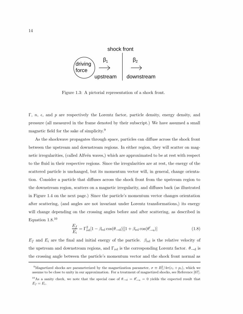
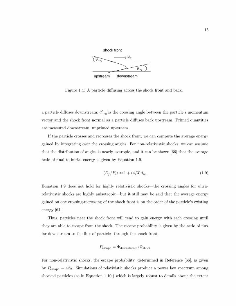
1.3 A pictorial representation of a shock front. . . . . . . . . . . . . . . . . . . . 14
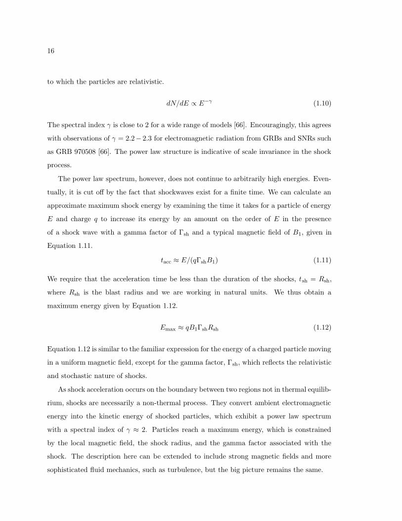
1.4 A particle diffusing across the shock front and back. . . . . . . . . . . . . . . 15
1.5 The Crab Nebula: the most famous plerion. The photo was taken by theHubble Space telescope [3]. . . . . . . . . . . . . . . . . . . . . . . . . . . . . 20
1.6 The Tycho SNR. The image is a false-color X-ray observation taken by theChandra experiment [4]. . . . . . . . . . . . . . . . . . . . . . . . . . . . . . 23
1.7 The active galaxy, Centaurus A. The optical image is courtesy the HubbleSpace Telescope; the false-color image (depicting the relativistic jets) is radiodata from the Very Large Array observatory [5]. . . . . . . . . . . . . . . . . 24
1.8 An image of GRB 990123 taken with the Hubble Space Telescope [6]. . . . . 27
2.1 Meson path length as a function of zenith angle. . . . . . . . . . . . . . . . . 35
2.2 The secant theta effect at 10GeV (left) and 1TeV (right). z=0 correspondsto horizontal and z=1 corresponds to vertical. . . . . . . . . . . . . . . . . . 36
2.3 On the left is the angle-averaged flux as calculated by a variety of groups.On the right is a linear plot of the ratio of different calculated fluxes to theBartol flux, with the solid line representing the Bartol flux and the short-longdashed line representing the Honda flux. (The figure is from Reference [7].) . 37
2.4 Muon neutrino survival probabilities as a function of cosine of zenith angleat three different energies. . . . . . . . . . . . . . . . . . . . . . . . . . . . . 39
2.5 The Earth’s neutrino shadow factor as a function of zenith angle in radiansat different energies (from Reference [8].) θ = 0 corresponds to vertical andθ = 1.57 corresponds to horizontal. . . . . . . . . . . . . . . . . . . . . . . . 40
2.6 Components of νN cross section scaled by 1/E (from Reference [9].) Theuncertainty is 20% up to 1PeV above which, the uncertainty may (conserva-tively) grow as large as 200% by 1012 eV. . . . . . . . . . . . . . . . . . . . . 42
iv
2.7 The Earth shadow as demonstrated by the differential upmu flux due to asimulated point source measured at two different zenith angles. The spectralindex is γ = 2 and the units of flux are arbitrary. . . . . . . . . . . . . . . . 43
3.1 Electric field lines for a non-relativistic particle (left) and for a highly rela-tivistic particle (right). . . . . . . . . . . . . . . . . . . . . . . . . . . . . . . 46
3.2 Electromagnetic field vectors at a characteristic distance b away from a rela-tivistic particle. . . . . . . . . . . . . . . . . . . . . . . . . . . . . . . . . . . 47
3.3 Determination of energy loss per unit track length. . . . . . . . . . . . . . . 48
3.4 Radiation for non-relativistic (left) and relativistic particles (right) in linearmedia. . . . . . . . . . . . . . . . . . . . . . . . . . . . . . . . . . . . . . . . 49
3.5 The location of the Super-Kamiokande experiment (from Reference [10].) . . 50
3.6 A sketch of the Super-Kamiokande detector situated in Mt. Ikeno (fromReference [10].) . . . . . . . . . . . . . . . . . . . . . . . . . . . . . . . . . . 52
3.7 A diagram of an ID PMT (from Reference [10].) . . . . . . . . . . . . . . . . 53
3.8 Quantum efficiency of the ID PMTs (from Reference [10].) They are maxi-mally efficient for UV light. . . . . . . . . . . . . . . . . . . . . . . . . . . . . 54
3.9 A simplified schematic diagram of a Super-Kamiokande ATM, which recordstime and charge information from ID PMTs. For a more comprehensivediagram, see Reference [10]. . . . . . . . . . . . . . . . . . . . . . . . . . . . 56
3.10 A simplified schematic diagram of the QTC module, used in the OD DAQto record time and charge information from OD PMTs. For a more compre-hensive diagram, see Reference [10]. . . . . . . . . . . . . . . . . . . . . . . . 57
3.11 Delay in OD DAQ digitization observed during high-energy calibration events(from Reference [11].) . . . . . . . . . . . . . . . . . . . . . . . . . . . . . . . 58
3.12 A diagram depicting the data captured by the ID and OD as a function oftime. Also, we show the time required to digitize the OD data. . . . . . . . . 59
3.13 The Super-Kamiokande water purification system, (from Reference [10].) . . 62
3.14 Measuring water transparency with the titanium-sapphire laser (from Refer-ence [10].) . . . . . . . . . . . . . . . . . . . . . . . . . . . . . . . . . . . . . 64
3.15 A graph of measured geometric photosensitivity (a) and a diagrammatic def-inition of θ (b) (from Reference [10].) . . . . . . . . . . . . . . . . . . . . . . 65
3.16 Q(l)/f(θ) as a function of path length (l) (from Reference [10].) . . . . . . . 66
3.17 Attenuation length as a function of run number for SK-III. One run typicallycorresponds to roughly one day of data. . . . . . . . . . . . . . . . . . . . . . 66
3.18 Laser measurement of the attenuation coefficients (top-left) and a typicalcalibration event (bottom-right.) (The image is from from Reference [10].) . 68
v
3.19 Above is a histogram of the photon arrival times for MC (bars) and calibrationdata (dots). The peak at 730 ns is due to scattered photons, while the secondsmaller peak at 1, 025 ns is due to the reflection of photons off the PMTs andblack sheet on the ID floor. Below is the difference between MC and data.Data and MC agree to within 2%. This calibration plot is for 337 nm laserlight and the figure is from from Reference [10]. . . . . . . . . . . . . . . . . 69
3.20 SK-I calibration measurements of attenuation length by laser (triangles) andby cosmic ray muons (diamonds) as a function of time (from Reference [10].)The two calibration techniques agree to within a few percent. . . . . . . . . 70
3.21 The xenon lamp used to measure PMT gain (from Reference [10].) . . . . . 71
3.22 Relative PMT gain (normalized by its mean) after recalibration (from Ref-erence [10].) . . . . . . . . . . . . . . . . . . . . . . . . . . . . . . . . . . . . 73
3.23 A typical TQ-map for a single ID PMT (from Reference [10].) The x-axishas a split scale that is linear up to 5 pe where it becomes logarithmic. . . . 74
3.24 The timing calibration system (from Reference [10].) . . . . . . . . . . . . . 74
3.25 Fiberglass enclosures (FRPs) for PMTs with acrylic caps (from Reference [12].)Dimensions are in mm. . . . . . . . . . . . . . . . . . . . . . . . . . . . . . . 76
4.1 A flowchart of Monte Carlo generation. . . . . . . . . . . . . . . . . . . . . . 79
4.2 The spectra of point source upmu for a source with spectral indices γ = 2and γ = 3 detected at z = 0.1. . . . . . . . . . . . . . . . . . . . . . . . . . . 83
4.3 The total average angular deflection between upmus created by parent neu-trinos characterized by a γ = 2 source and detected at z = 0.1. . . . . . . . . 85
5.1 Upmu production through charged current scattering. . . . . . . . . . . . . . 87
5.2 Upmu classification. . . . . . . . . . . . . . . . . . . . . . . . . . . . . . . . . 88
5.3 Neutrino energies by event type in SK-III MC. . . . . . . . . . . . . . . . . . 89
5.4 Muon energies by event type in SK-III MC. . . . . . . . . . . . . . . . . . . . 89
5.5 A schematic overview of the reduction. . . . . . . . . . . . . . . . . . . . . . 91
5.6 A schematic of the umred1st reduction. The UHE threshold was lowered to.80 × 106 pe for SK-II. . . . . . . . . . . . . . . . . . . . . . . . . . . . . . . . 94
5.7 A schematic of the umred2nd reduction. . . . . . . . . . . . . . . . . . . . . 99
5.8 Angular separation between true muon direction and the reconstructed di-rection as determined by the precise fitter using SK-III MC. All histogramsare normalized to one. (Showering events are discussed in greater detail inSection 5.6.) . . . . . . . . . . . . . . . . . . . . . . . . . . . . . . . . . . . . 100
5.9 Angular resolution as a function of true muon energy for SK-III MC. . . . . 101
vi
5.10 Angular resolution as a function of zenith angle using SK-III MC. Each datapoint includes contributions from stopping, thru, and showering muons. Theprecise fitter performs best for slightly upward-going muons, and worst forstraight upward-going muons. . . . . . . . . . . . . . . . . . . . . . . . . . . 102
5.11 True momentum (at entry point) minus reconstructed momentum for SK-IIIstopping muons. . . . . . . . . . . . . . . . . . . . . . . . . . . . . . . . . . . 104
5.12 Hit OD PMTs within 8m of the fit entry point. Events with 10 or more hitsare considered thru; those with less than 10 are considered stopping. . . . . 105
5.13 A comparison of track length for data (points) and MC (bars) for SK-II.The black vertical black line at 700 cm represents the upmu path length cutand the adjacent vertical red lines represent systematic uncertainty in thedetermination of track length. . . . . . . . . . . . . . . . . . . . . . . . . . . 106
5.14 Determination of reconstructed length resolution using shifted histograms. . 107
5.15 Muon energy loss per unit track length as a function of energy (from Refer-ence [13].) . . . . . . . . . . . . . . . . . . . . . . . . . . . . . . . . . . . . . 109
5.16 Showering tuning plots for SK-III. Data is plotted as points with error barsand MC is plotted as bars. . . . . . . . . . . . . . . . . . . . . . . . . . . . . 111
5.17 A scatterplot of ∆ and χ2 for SK-I MC showering (left) and non-showeringmuons (right) from Reference [14]. . . . . . . . . . . . . . . . . . . . . . . . . 112
5.18 A multiple-muon event represented with idraw. The solid red line is theprecise fit. . . . . . . . . . . . . . . . . . . . . . . . . . . . . . . . . . . . . . 113
5.19 A true upmu from the SK-III dataset. Hit clusters are clearly visible in theOD display in the upper-left-hand corner. . . . . . . . . . . . . . . . . . . . . 116
5.20 A true upmu from the SK-I dataset represented with the superscan program.Red and blue pixels respectively indicate large and small charge deposition.Information from the OD is displayed in the upper-right-hand corner. . . . . 117
5.21 A pictorial representation of live time. . . . . . . . . . . . . . . . . . . . . . 119
5.22 Upmu detection efficiency as a function of zenith angle. . . . . . . . . . . . . 121
5.23 A profile of the rock thickness around Super-Kamiokande (from Reference [15].)The origin is the center of detector. . . . . . . . . . . . . . . . . . . . . . . . 123
5.24 A downward going muon parametrized with Super-Kamiokande coordinates. 123
5.25 A scatter plot of z = cos(θ) and φ. The red horizontal line marks the divisionbetween downward-going and upward-going muons and the blue vertical linesdemarcate Region 1 and Region 2. . . . . . . . . . . . . . . . . . . . . . . . . 124
5.26 A histogram of φ for all muons with z > −0.1 (unshaded) and a histogramof φ for only muons with z > 0 (shaded). . . . . . . . . . . . . . . . . . . . . 125
5.27 Fit of zenith angle distributions for nearly-horizontal cosmic rays in Region2 for SK-III. Superimposed red circles are the data from Region 1. . . . . . . 127
vii
6.1 The search cone. . . . . . . . . . . . . . . . . . . . . . . . . . . . . . . . . . . 131
6.2 Using through-going muons from point source MC, we determined the RMSfor θ varied by as much as 0.5 between SK-I and SK-II. Recall that θ includescontributions from νµ scattering as well as detector resolution. . . . . . . . . 133
6.3 A histogram of αF generated from atmospheric (background) MC with searchdirections spaced at 4 intervals. α is often fit to 0 (no signal). . . . . . . . . 135
6.4 A histogram of nS generated from background MC with search directionsspaced at 4 intervals. . . . . . . . . . . . . . . . . . . . . . . . . . . . . . . . 136
6.5 Case 1: the lower limit of the integral runs into the barrier of physicality atα = 0. . . . . . . . . . . . . . . . . . . . . . . . . . . . . . . . . . . . . . . . . 137
6.6 Case 2: the integral does not run into a barrier of physicality. . . . . . . . . 137
6.7 A distribution of x (the upper limit on α at 90% CL) generated from back-ground MC with search directions spaced at 4 intervals. . . . . . . . . . . . 138
6.8 A distribution of nxS from background MC with search directions spaced at
4 intervals. . . . . . . . . . . . . . . . . . . . . . . . . . . . . . . . . . . . . 139
6.9 A map of point source upmu flux limits -[log10(cm−2s−1)] for background MC
with search directions spaced at 0.5 intervals. The dotted line is the galacticplane. . . . . . . . . . . . . . . . . . . . . . . . . . . . . . . . . . . . . . . . . 139
6.10 A histogram of Λ generated using a single background MC sky map withsearch directions spaced at 4 intervals. There is an excess of events withΛ = 0 due to the tendency for αF to be zero. . . . . . . . . . . . . . . . . . . 141
6.11 A normalized histogram of Λmax generated using atmospheric backgroundMC. The thresholds for 90%/99% detection are respectively indicated withred and green vertical lines. Search directions are spaced at 0.5 intervals. . 142
6.12 A histogram of Λ generated using a combination of atmospheric backgroundand point source signal MC at the point (ra,dec)=(110,−15). The signalsize (13 upmus) has been adjusted so that the detection rate is approximately90%. The threshold for detection at 90% CL is marked with a red line. . . . . 143
6.13 An atmospheric (background) MC sky map of Λ with search directions spacedat 0.5 intervals. The dotted line is the galactic plane. . . . . . . . . . . . . 146
6.14 A MC sky map of Λ combining background with enough signal for detectionat > 99% CL. The source is located at (dec,ra)=(−45, 110). The searchdirections are spaced at 0.5 intervals. The dotted line is the galactic plane. 146
6.15 The point spread function at two different different regions of zenith angle. . 148
6.16 The point spread function S(θ...) for through-going and showering muons.Each distribution is normalized to one, and vertical error bars—though included—are too small to see. . . . . . . . . . . . . . . . . . . . . . . . . . . . . . . . . 149
6.17 Distributions of t used to generate random values of local sidereal time forMC simulations. . . . . . . . . . . . . . . . . . . . . . . . . . . . . . . . . . . 150
viii
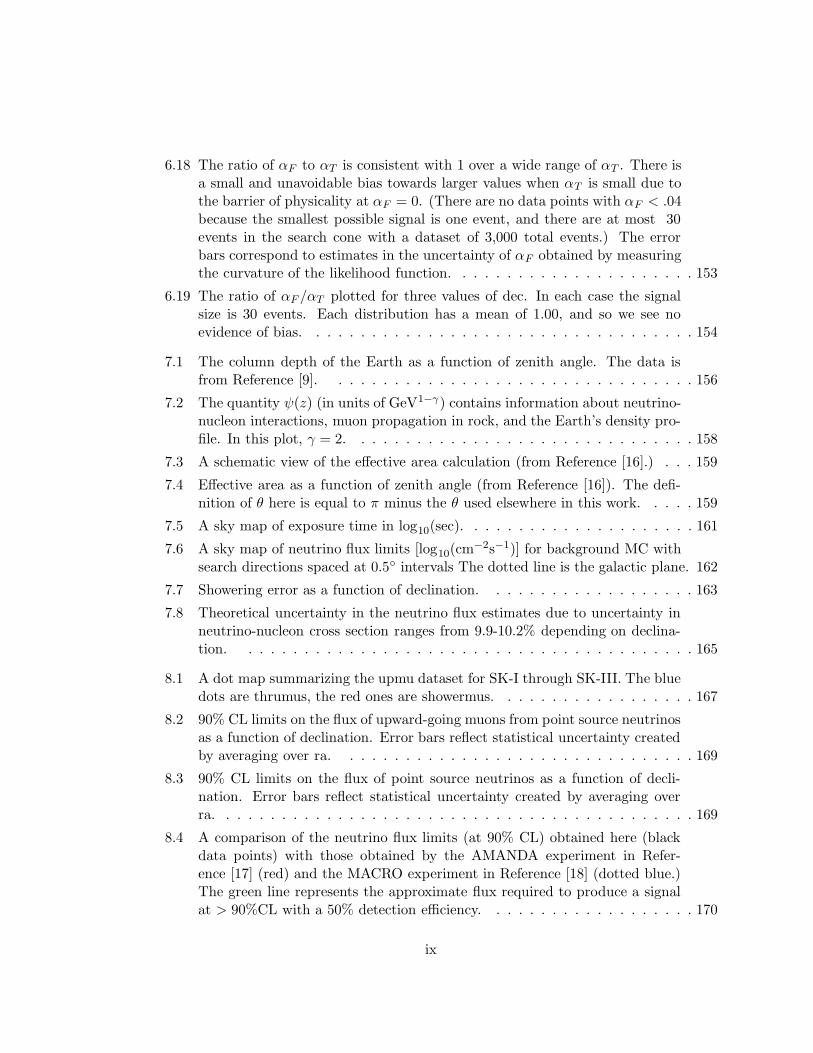
6.18 The ratio of αF to αT is consistent with 1 over a wide range of αT . There isa small and unavoidable bias towards larger values when αT is small due tothe barrier of physicality at αF = 0. (There are no data points with αF < .04because the smallest possible signal is one event, and there are at most 30events in the search cone with a dataset of 3,000 total events.) The errorbars correspond to estimates in the uncertainty of αF obtained by measuringthe curvature of the likelihood function. . . . . . . . . . . . . . . . . . . . . . 153
6.19 The ratio of αF /αT plotted for three values of dec. In each case the signalsize is 30 events. Each distribution has a mean of 1.00, and so we see noevidence of bias. . . . . . . . . . . . . . . . . . . . . . . . . . . . . . . . . . . 154
7.1 The column depth of the Earth as a function of zenith angle. The data isfrom Reference [9]. . . . . . . . . . . . . . . . . . . . . . . . . . . . . . . . . 156
7.2 The quantity ψ(z) (in units of GeV1−γ) contains information about neutrino-nucleon interactions, muon propagation in rock, and the Earth’s density pro-file. In this plot, γ = 2. . . . . . . . . . . . . . . . . . . . . . . . . . . . . . . 158
7.3 A schematic view of the effective area calculation (from Reference [16].) . . . 159
7.4 Effective area as a function of zenith angle (from Reference [16]). The defi-nition of θ here is equal to π minus the θ used elsewhere in this work. . . . . 159
7.5 A sky map of exposure time in log10(sec). . . . . . . . . . . . . . . . . . . . . 161
7.6 A sky map of neutrino flux limits [log10(cm−2s−1)] for background MC with
search directions spaced at 0.5 intervals The dotted line is the galactic plane. 162
7.7 Showering error as a function of declination. . . . . . . . . . . . . . . . . . . 163
7.8 Theoretical uncertainty in the neutrino flux estimates due to uncertainty inneutrino-nucleon cross section ranges from 9.9-10.2% depending on declina-tion. . . . . . . . . . . . . . . . . . . . . . . . . . . . . . . . . . . . . . . . . 165
8.1 A dot map summarizing the upmu dataset for SK-I through SK-III. The bluedots are thrumus, the red ones are showermus. . . . . . . . . . . . . . . . . . 167
8.2 90% CL limits on the flux of upward-going muons from point source neutrinosas a function of declination. Error bars reflect statistical uncertainty createdby averaging over ra. . . . . . . . . . . . . . . . . . . . . . . . . . . . . . . . 169
8.3 90% CL limits on the flux of point source neutrinos as a function of decli-nation. Error bars reflect statistical uncertainty created by averaging overra. . . . . . . . . . . . . . . . . . . . . . . . . . . . . . . . . . . . . . . . . . . 169
8.4 A comparison of the neutrino flux limits (at 90% CL) obtained here (blackdata points) with those obtained by the AMANDA experiment in Refer-ence [17] (red) and the MACRO experiment in Reference [18] (dotted blue.)The green line represents the approximate flux required to produce a signalat > 90%CL with a 50% detection efficiency. . . . . . . . . . . . . . . . . . . 170
ix
8.5 A sky map of 90% CL muon flux limits -[log10(cm−2s−1)]. The dotted line is
the galactic plane. . . . . . . . . . . . . . . . . . . . . . . . . . . . . . . . . . 171
8.6 A sky map of 90% CL neutrino flux limits -[log10(cm−2s−1)]. The dotted line
is the galactic plane. . . . . . . . . . . . . . . . . . . . . . . . . . . . . . . . 171
8.7 A sky map of Λ. The maximum value (Λmax = 19.1) is below the detectionthreshold. The dotted line is the galactic plane. . . . . . . . . . . . . . . . . 172
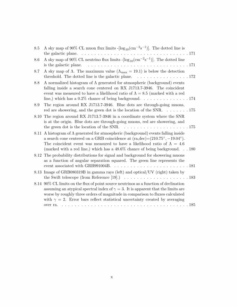
8.8 A normalized histogram of Λ generated for atmospheric (background) eventsfalling inside a search cone centered on RX J1713.7-3946. The coincidentevent was measured to have a likelihood ratio of Λ = 8.5 (marked with a redline,) which has a 0.2% chance of being background. . . . . . . . . . . . . . . 174
8.9 The region around RX J1713.7-3946. Blue dots are through-going muons,red are showering, and the green dot is the location of the SNR. . . . . . . . 175
8.10 The region around RX J1713.7-3946 in a coordinate system where the SNRis at the origin. Blue dots are through-going muons, red are showering, andthe green dot is the location of the SNR. . . . . . . . . . . . . . . . . . . . . 175
8.11 A histogram of Λ generated for atmospheric (background) events falling insidea search cone centered on a GRB coincidence at (ra,dec)=(210.75 ,−19.04).The coincident event was measured to have a likelihood ratio of Λ = 4.6(marked with a red line,) which has a 48.6% chance of being background. . . 180
8.12 The probability distributions for signal and background for showering muonsas a function of angular separation squared. The green line represents theevent associated with GRB991004B. . . . . . . . . . . . . . . . . . . . . . . . 181
8.13 Image of GRB080319B in gamma rays (left) and optical/UV (right) taken bythe Swift telescope (from Reference [19].) . . . . . . . . . . . . . . . . . . . . 183
8.14 90% CL limits on the flux of point source neutrinos as a function of declinationassuming an atypical spectral index of γ = 3. It is apparent that the limits areworse by roughly three orders of magnitude in comparison to fluxes calculatedwith γ = 2. Error bars reflect statistical uncertainty created by averagingover ra. . . . . . . . . . . . . . . . . . . . . . . . . . . . . . . . . . . . . . . . 185
x
LIST OF TABLES
Table Number Page
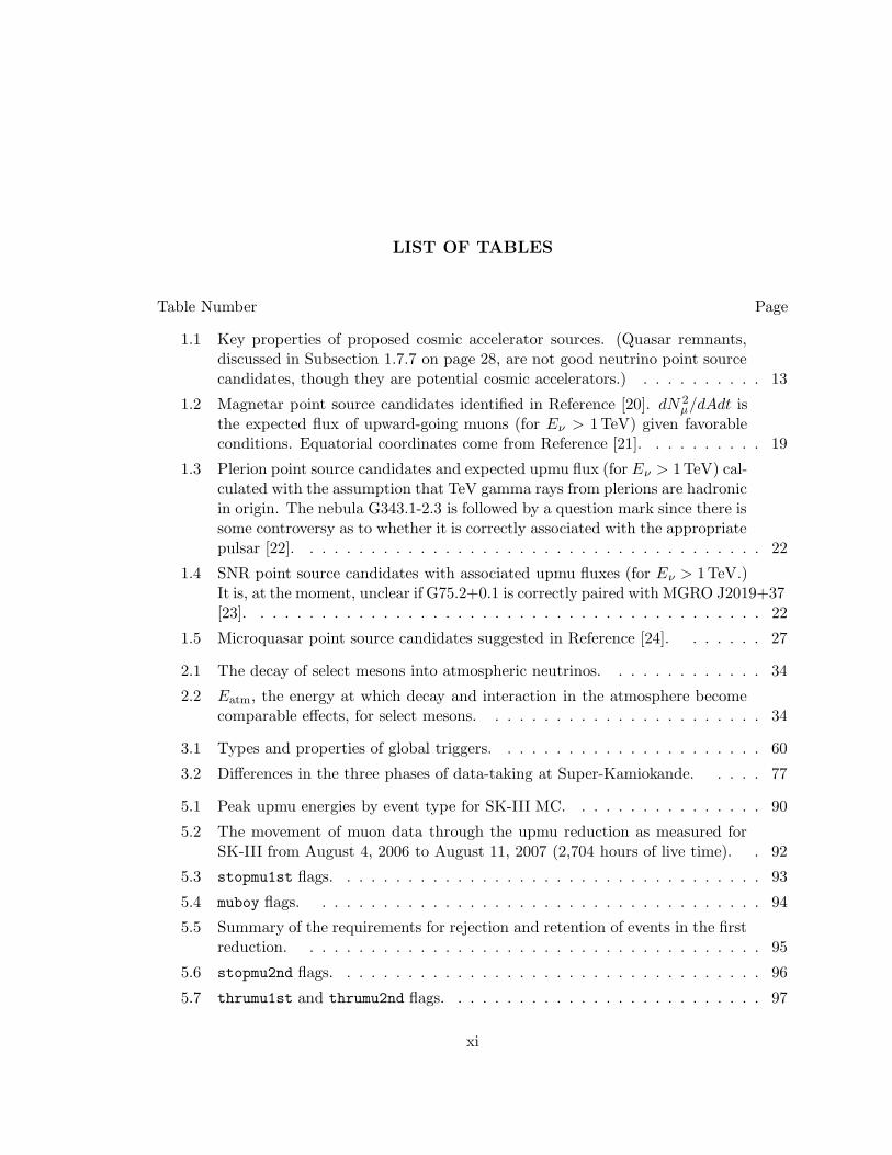
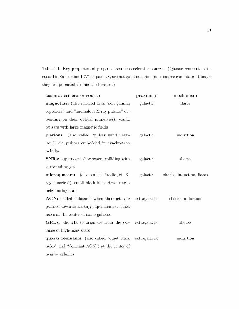
1.1 Key properties of proposed cosmic accelerator sources. (Quasar remnants,discussed in Subsection 1.7.7 on page 28, are not good neutrino point sourcecandidates, though they are potential cosmic accelerators.) . . . . . . . . . . 13
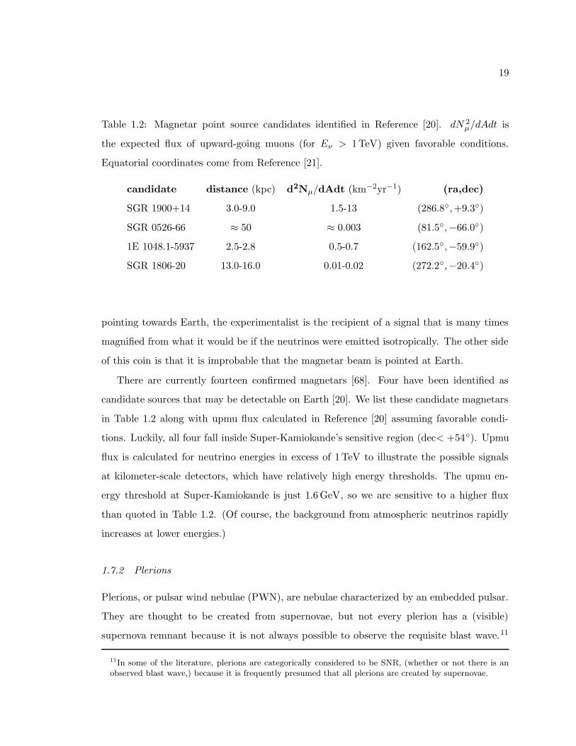
1.2 Magnetar point source candidates identified in Reference [20]. dN 2µ/dAdt is
the expected flux of upward-going muons (for Eν > 1TeV) given favorableconditions. Equatorial coordinates come from Reference [21]. . . . . . . . . . 19
1.3 Plerion point source candidates and expected upmu flux (for Eν > 1TeV) cal-culated with the assumption that TeV gamma rays from plerions are hadronicin origin. The nebula G343.1-2.3 is followed by a question mark since there issome controversy as to whether it is correctly associated with the appropriatepulsar [22]. . . . . . . . . . . . . . . . . . . . . . . . . . . . . . . . . . . . . . 22
1.4 SNR point source candidates with associated upmu fluxes (for Eν > 1TeV.)It is, at the moment, unclear if G75.2+0.1 is correctly paired with MGRO J2019+37[23]. . . . . . . . . . . . . . . . . . . . . . . . . . . . . . . . . . . . . . . . . . 22
1.5 Microquasar point source candidates suggested in Reference [24]. . . . . . . 27
2.1 The decay of select mesons into atmospheric neutrinos. . . . . . . . . . . . . 34
2.2 Eatm, the energy at which decay and interaction in the atmosphere becomecomparable effects, for select mesons. . . . . . . . . . . . . . . . . . . . . . . 34
3.1 Types and properties of global triggers. . . . . . . . . . . . . . . . . . . . . . 60
3.2 Differences in the three phases of data-taking at Super-Kamiokande. . . . . 77
5.1 Peak upmu energies by event type for SK-III MC. . . . . . . . . . . . . . . . 90
5.2 The movement of muon data through the upmu reduction as measured forSK-III from August 4, 2006 to August 11, 2007 (2,704 hours of live time). . 92
5.3 stopmu1st flags. . . . . . . . . . . . . . . . . . . . . . . . . . . . . . . . . . . 93
5.4 muboy flags. . . . . . . . . . . . . . . . . . . . . . . . . . . . . . . . . . . . . 94
5.5 Summary of the requirements for rejection and retention of events in the firstreduction. . . . . . . . . . . . . . . . . . . . . . . . . . . . . . . . . . . . . . 95
5.6 stopmu2nd flags. . . . . . . . . . . . . . . . . . . . . . . . . . . . . . . . . . . 96
5.7 thrumu1st and thrumu2nd flags. . . . . . . . . . . . . . . . . . . . . . . . . . 97
xi
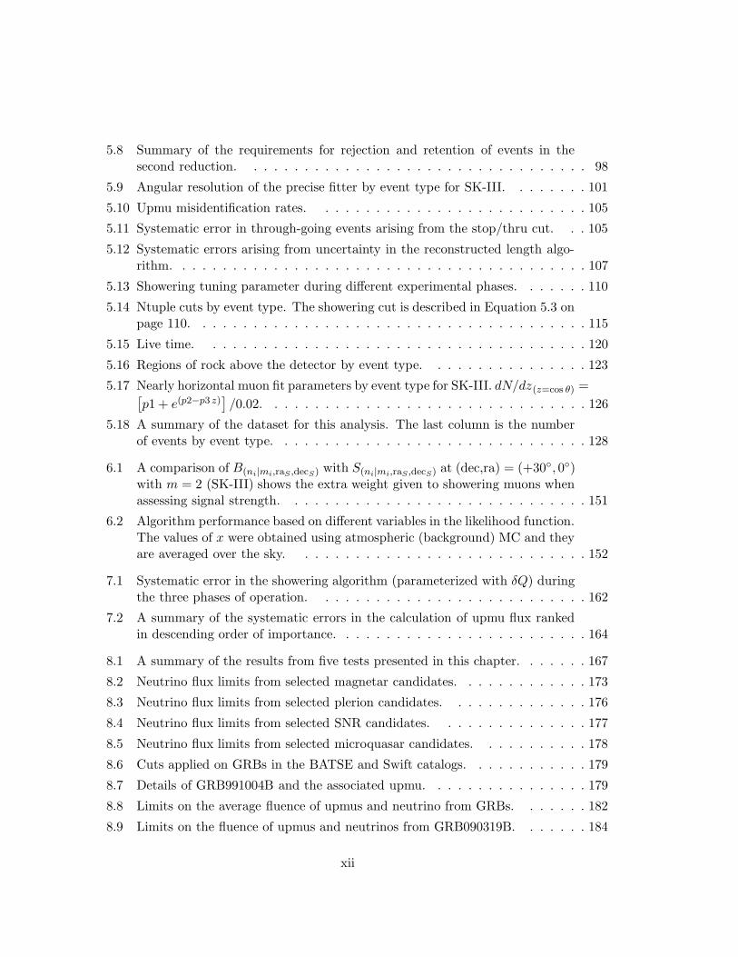
5.8 Summary of the requirements for rejection and retention of events in thesecond reduction. . . . . . . . . . . . . . . . . . . . . . . . . . . . . . . . . . 98
5.9 Angular resolution of the precise fitter by event type for SK-III. . . . . . . . 101
5.10 Upmu misidentification rates. . . . . . . . . . . . . . . . . . . . . . . . . . . 105
5.11 Systematic error in through-going events arising from the stop/thru cut. . . 105
5.12 Systematic errors arising from uncertainty in the reconstructed length algo-rithm. . . . . . . . . . . . . . . . . . . . . . . . . . . . . . . . . . . . . . . . . 107
5.13 Showering tuning parameter during different experimental phases. . . . . . . 110
5.14 Ntuple cuts by event type. The showering cut is described in Equation 5.3 onpage 110. . . . . . . . . . . . . . . . . . . . . . . . . . . . . . . . . . . . . . . 115
5.15 Live time. . . . . . . . . . . . . . . . . . . . . . . . . . . . . . . . . . . . . . 120
5.16 Regions of rock above the detector by event type. . . . . . . . . . . . . . . . 123
5.17 Nearly horizontal muon fit parameters by event type for SK-III. dN/dz(z=cos θ) =[
p1 + e(p2−p3 z)]
/0.02. . . . . . . . . . . . . . . . . . . . . . . . . . . . . . . . 126
5.18 A summary of the dataset for this analysis. The last column is the numberof events by event type. . . . . . . . . . . . . . . . . . . . . . . . . . . . . . . 128
6.1 A comparison of B(ni|mi,raS ,decS) with S(ni|mi,raS ,decS) at (dec,ra) = (+30, 0)with m = 2 (SK-III) shows the extra weight given to showering muons whenassessing signal strength. . . . . . . . . . . . . . . . . . . . . . . . . . . . . . 151
6.2 Algorithm performance based on different variables in the likelihood function.The values of x were obtained using atmospheric (background) MC and theyare averaged over the sky. . . . . . . . . . . . . . . . . . . . . . . . . . . . . 152
7.1 Systematic error in the showering algorithm (parameterized with δQ) duringthe three phases of operation. . . . . . . . . . . . . . . . . . . . . . . . . . . 162
7.2 A summary of the systematic errors in the calculation of upmu flux rankedin descending order of importance. . . . . . . . . . . . . . . . . . . . . . . . . 164
8.1 A summary of the results from five tests presented in this chapter. . . . . . . 167
8.2 Neutrino flux limits from selected magnetar candidates. . . . . . . . . . . . . 173
8.3 Neutrino flux limits from selected plerion candidates. . . . . . . . . . . . . . 176
8.4 Neutrino flux limits from selected SNR candidates. . . . . . . . . . . . . . . 177
8.5 Neutrino flux limits from selected microquasar candidates. . . . . . . . . . . 178
8.6 Cuts applied on GRBs in the BATSE and Swift catalogs. . . . . . . . . . . . 179
8.7 Details of GRB991004B and the associated upmu. . . . . . . . . . . . . . . . 179
8.8 Limits on the average fluence of upmus and neutrino from GRBs. . . . . . . 182
8.9 Limits on the fluence of upmus and neutrinos from GRB090319B. . . . . . . 184
xii
C.1 The number of events during each experimental phase. The relatively highnumber of showering muons during SK-II reflects the diminished performanceof the algorithm with fewer phototubes. . . . . . . . . . . . . . . . . . . . . . 205
C.2 Arrays and associated header files . . . . . . . . . . . . . . . . . . . . . . . . 206
C.3 Arrays and associated header files . . . . . . . . . . . . . . . . . . . . . . . . 206
xiii

GLOSSARY
AGN: Active Galactic Nucleus
ATM: Analog Timing Module
AXP: Anomalous X-Ray Pulsar
BIP: Busy In Progress (BIP) time occurs when there are two high-energy triggers within
8 − 56µs of each other.
CORNER-CLIPPER: A muon event, which is difficult to reconstruct because its track clips
the corner of the ID.
CL: Confidence level
CMB: Cosmic Microwave Background
CSS: Compact Steep Spectrum
DAQ: Data Acquisition
DEC: Declination
FRP: Fiber Reinforced Plastic (cases for ID PMTs)
GPS: GHz Peaked Source and also Global Positioning System (depending on context)
GRB: Gamma Ray Burst
xiv

ID: Inner Detector
IRAS: Infra-Red Astronomical Satellite
LDPE: Low-Density Polyethylene
MC: Monte Carlo
MWE: Meters water equivalent
MULTI-MU: An event caused by several muons passing through the detector at approxi-
mately the same. These events can be difficult to reconstruct.
PSF: Point Spread Function
OD: Outer Detector
PC/FC: Partially Contained / Fully Contained
PE: Photoelectrons
PMT: Photomultiplier Tube
PWN: Pulsar Wind Nebula
QAC: Charge-to-Analog Converter
QTC: Charge-to-Time Converter
RA: Right ascension
SGR: Soft Gamma Repeater
SNR: Supernova Remnant
xv

SK: Super-Kamiokande
STOPPER: An upward-going muon, which stops in the detector. These events are the
lowest energy category of upward-going muons.
TAC: Time-to-Analog Converter
THRU: An upward-going muon, with both entry and exit points. Through-going muons
are further divided into showering and non-showering categories, which represent
the first and second most energetic categories of upward-going muons at Super-
Kamiokande.
THRUMU: See “thru.”
UHE: Ultra-High-Energy
UPMU: Upward-going muon caused by a neutrino interaction in the rock below and
around the detector.
xvi
ACKNOWLEDGMENTS
I would like to first thank Jeff Wilkes for advising me through five years of graduate
school. Through his mentorship I was able to work halfway around the world on the world’s
largest water Cherenkov detector at a very exciting time in neutrino physics. Through
his teaching and anecdotes, he helped me develop a healthy experimentalist’s instinct for
skepticism while providing me with useful tools for analysis and design. He went to great
lengths to help me build connections with other physicists and to plan for my future.
Though technically I had only one advisor, I was very lucky to regularly benefit from the
sage advice of two additional professors who I should also like to call advisors. Alec Habig
helped me find my bearings when I was most in need direction. He listened to my ideas
and made suggestions when my research was in its infancy. His patience and helpfulness
helped me develop a basic algorithm, which I could use as a starting point. I am likewise
deeply indebted to Toby Burnett for his advice on statistical techniques. He met with me
regularly and helped me turn my basic algorithm into something far more sophisticated. I
will always appreciate his patience and encouragement.
I would like to thank the other members of my committee for reviewing my thesis research
and giving me valuable advice: Jens Gundlach, Leslie Rosenberg, Wick Haxton, and Scott
Anderson. I also thank Cecilia Lunardini for introducing me to theoretical concepts in
neutrino physics. Her instruction broadened my understanding and appreciation for particle
physics.
I am also deeply grateful for help from my colleagues at Super-Kamiokande. I thank
Yoshitaka Itow, Takaaki Kajita, Ed Kearns, John Learned, Shigetaka Moriyama, Kate
Scholberg, and Larry Sulak for taking the time to give me comments on my research. Jen
Raaf was tremendously helpful over the course of my graduate career, and I benefited greatly
from her leadership of the upward-going muon subgroup. She taught me about coding,
xvii

about the Super-Kamiokande data reduction process, and helped me hunt down bugs and
missing files. Yosh Shiraishi was another helpful mentor early in my graduate career. He
answered my computing questions, helped me plan my first trips to Japan, and studied
neutrino phenomenology with me. I thank Hans Berns for answering all of my hardware
and technical questions. I thank Shantanu Desai for sharing his expertise on showering
muons with me. I thank Molly Swanson for providing me with tables and documentation
for the calculation of neutrino flux.
I also wish to thank Chris Regis, Roger Wendell, Mike Litos, and fellow upmu member,
Tanaka Takayuki, for assistance with Super-Kamiokande software. I thank Mike Dziomba
and Kevin Connolly for their comments on my thesis.
Obtaining my doctoral degree has been the most challenging undertaking in my life to
date and I am thankful for the support of my family. I thank my parents for their advice
and encouragement. I thank them for teaching me to always do my best. I thank my wife,
Megan, for keeping life in perspective, for sharing my passion for science, and for always
believing in me.
xviii
1
Chapter 1
THEORETICAL MOTIVATION FOR NEUTRINO POINT SOURCES
1.1 Definition and Overview
Neutrino point sources are distant objects that produce copious high-energy neutrinos (in
excess of 1GeV.) They may be either galactic or extragalactic. From Earth, they should
appear to be pointlike. At the present time, there is no direct observational evidence for
the existence of neutrino point sources, but they are a feature of several scenarios in ultra-
high-energy (UHE) astronomy. Most of these scenarios involve the emission of high-energy
neutrinos, which distinguish these sources from lower energy (MeV-scale) sources such as
the sun and nearby supernovae, which are both, technically speaking, pointlike using current
detection methods (due to the scattering angle between a neutrino and its daughter muon
at low energies, and due to limits on current detector resolution at high energies.) In this
work we study high-energy point sources, which we shall refer to as simply “point sources.”
In Section 1.2, we describe the current trends in neutrino astronomy. In Section 1.3 we
discuss the related subject of UHE cosmic rays. In Section 1.4, we elucidate the connection
between recent developments in UHE cosmic ray astronomy and neutrino astronomy. In
doing so, we hope to impart to the reader that the search for neutrino point sources is an
important and exciting project that we can reasonably expect to yield conclusive results in
the foreseeable future. In Section 1.5, we distinguish two categories of neutrino point sources:
bottom-up and top-down. Then, in Section 1.6, we focus on bottom-up scenarios, also called
“cosmic accelerator” models, which make well-constrained predictions about point source
neutrino flux, invoking only standard model physics. In this section we will explore the
related phenomena of shocks. In Section 1.7, we will explore promising candidates for
neutrino point sources such as active galactic nuclei and pulsar wind nebulae. We conclude
2
the chapter with a discussion of related experiments in Section 1.8.
1.2 Current Trends in Neutrino Astronomy
Construction is underway at the South Pole where the IceCube experiment is on target to
become the world’s first kilometer-sized neutrino detector [25]. (Barring delays, construction
is expected to be completed in 2011.) Three experiments in the Mediterranean, meanwhile,
have united to design a second and complementary kilometer-sized neutrino detector in the
northern hemisphere [26]. Other large detectors have been proposed in the US and Japan
[27][28]. These experiments are not cheap; the IceCube experiment has a project cost of
$272 million [29]. Clearly, neutrino astronomy has become high-priority research.
Advocates have pointed out several assets unique to the field of neutrino astronomy:
[30]
• Due to their low cross section, the universe is transparent to neutrinos over a wide
range of energies, and this opens the door for exciting possibilities. Neutrinos may
allow us to “see through” quasi-opaque objects such as the galactic plane, or to “see
the inside” of an exploding star. The same may not be said of photons and protons,
which scatter off the cosmic microwave background among other things.
• Neutrinos are electrically neutral, and so their path is not affected by magnetic fields
as is the case with protons and charged nuclei. Thus, neutrinos point back to their
sources.
• Neutrinos are produced in generic situations where there is a high density hadronic
energy, and so they are correlated with photon and proton emission.
Two developments have been crucial in driving recent interest in neutrino astronomy.
First, there has been a realization, beginning with the first detection of neutrinos from the
sun [31], and culminating in the observation of neutrinos from SN1987A [32], that experi-
ments can overcome the difficulties created by the neutrino’s extremely small cross section,
and thereby observe a significant number of neutrinos from astrophysical sources. Second,
3
the idea has caught on that neutrino astronomy is likely to provide insight into other pressing
research problems, especially the origin of UHE cosmic rays, (see, e.g., Reference [33].)
As the idea of large scale neutrino telescopes has gained a foothold, there has been a
flurry of papers suggesting additional opportunities afforded by neutrino astronomy such as:
neutrinos from WIMPS [34], primordial black holes evaporation [35], and topological defects
[36]; non-perturbative W/Z production via UHE neutrinos [37], unexpected resonances in
the neutrino cross section (due to, e.g., the existence of a scalar leptoquark [38],) “Z-bursts”
from UHE neutrinos scattering on the relic neutrinos from the Big Bang [39], and direct
neutrino mass measurements from periodic sources [40]. We shall discuss some of these
scenarios in greater detail in Section 1.5.
1.3 An Introduction to UHE Cosmic Rays
1.3.1 Cosmic Accelerators and the Hillas Condition
UHE cosmic rays exceeding 106 GeV = 1PeV were first detected by Pierre Auger and
his collaborators in 1939 [41]. Subsequent experiments probed higher energies, and by
1963 there was evidence of cosmic rays with energies of 1011 GeV = 100EeV [42]. (For
comparison, the LHC hopes to generate proton beams with energies of 7, 000GeV = 7TeV.)
With the detection of UHE cosmic rays came three readily-apparent questions. Where do
UHE cosmic rays originate, by what mechanism do they gain such immense energy, and
what can they teach us about the universe?
The simplest explanation of UHE cosmic rays, which invokes no new physical laws
or particles, is that cosmic rays are accelerated by electromagnetic fields. This theory is
sometimes called “the cosmic accelerator model.” In a 1984 review of UHE cosmic rays,
A. M. Hillas pointed out that we can use the Larmor radius, (which defines the radius of
the circular motion of a charged particle in a uniform magnetic field,) to constrain the size
of the region wherein cosmic rays undergo acceleration [1]. The condition, known as “the
Hillas condition,” is:
E < qBR (1.1)
where E, q,B, and R are energy, charge, magnetic field, and Larmor radius respectively. In
4
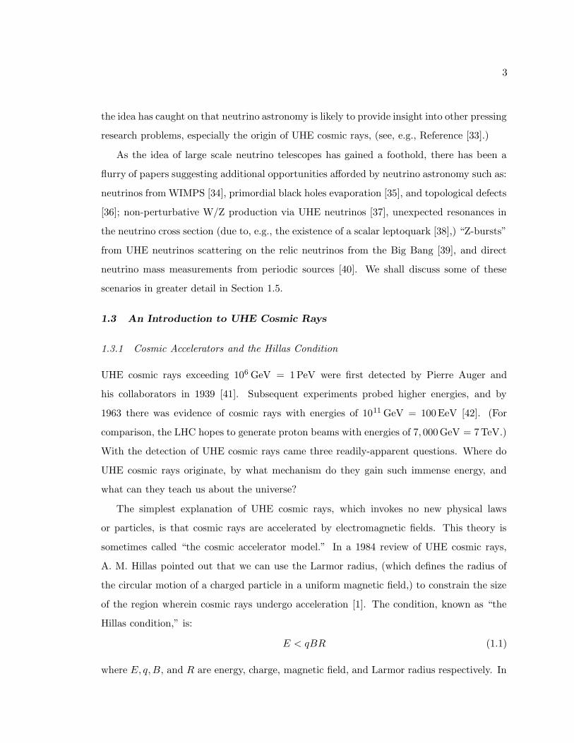
Figure 1.1: The original plot of magnetic field versus Larmor radius from Hillas’ 1984 review
[1]. Objects below the diagonal line cannot accelerate protons to 1020 eV.
what has become a canonical plot, (shown in Figure 1.1,) Hillas plotted magnetic field versus
Larmor radius for a variety of astronomical objects considered at the time of publication to
be candidates for UHE cosmic ray creation.1
A good deal of interesting information is contained in this plot. For one, it is apparent
that small accelerators require compensatingly large magnetic fields, whereas large accel-
erators require more modest magnetic fields. Below the diagonal line, protons can not be
accelerated to 1020 eV. If we lower the energy requirement, (or raise the charge of the cosmic
ray,) the y-intercept of the exclusion line becomes smaller. It is also apparent that objects
such as supernova remnants (SNRs) can accelerate cosmic rays to very high energies, even
though they are not capable of creating the highest energy cosmic rays. Indeed, relatively
few known objects can account UHE cosmic rays.
1Distant magnetic fields can be inferred using Zeeman splitting, or in the case of neutron stars, theslowdown of the period as a function of time.
5
1.3.2 Spectrum
The cosmic ray spectrum has been measured over many magnitudes of energy and is well de-
scribed as a slowly-varying power law. There are two notable features. The first, called “the
knee,” occurs at approximately 1015 eV. Here the spectral index steepens from 2.7 to about
3.1. The second feature, called “the ankle,” occurs at approximately 3×10¹⁸ eV, and marks
a flattening in the spectrum. It is commonly accepted that cosmic rays above the knee2
originate in galactic supernova remnants through Fermi shocks (see Subsection 1.6.2 on
page 12.) Cosmic rays above the ankle are also thought to be galactic in origin, and may
originate in objects such as pulsars. Cosmic rays below the ankle are thought to be extra-
galactic as there are no plausible galactic sources that meet the Hillas condition for such
high energies.
Restricting our attention for the moment to cosmic accelerator models, the leading
contender for UHE cosmic rays below the ankle are active galactic nuclei (AGN). Recent
evidence from the Auger experiment supports this theory [43]. Other possible sources,
discussed in Section 1.6, include pulsars and microquasars in our own galaxy, gamma ray
bursts (GRBs), active galactic nuclei, quasar remnants, and colliding galaxies [44].
1.3.3 The GZK Cutoff
Conventional wisdom tells us that the cosmic ray spectrum does not continue indefinitely,
but that it terminates at 6× 10¹⁹ GeV due to an effect dubbed “the GZK cutoff.” In 1966,
Greisen [45] and Zatsepin & Kuzmin [46] demonstrated that sufficiently UHE cosmic rays
above ≈ 1019 eV are highly prone to scatter off the cosmic microwave background (CMB)—
which is blue-shifted in their reference frame—in a reaction that produces a pion.
p+ + γ → π0 + p+ (1.2)
Thus a proton propagating through the CMB will steadily lose energy through pion pro-
duction until its energy falls below the GZK cutoff. Thus, we expect a “pileup” in the tail
of spectra from distant sources [44] from the energy loss of cosmic rays above the GZK
2We use the phrase “above the knee” in the anatomical sense, which is to say “possessing lower energythan particles at the knee.”
6
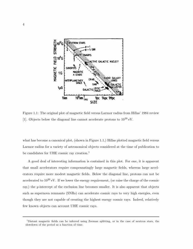
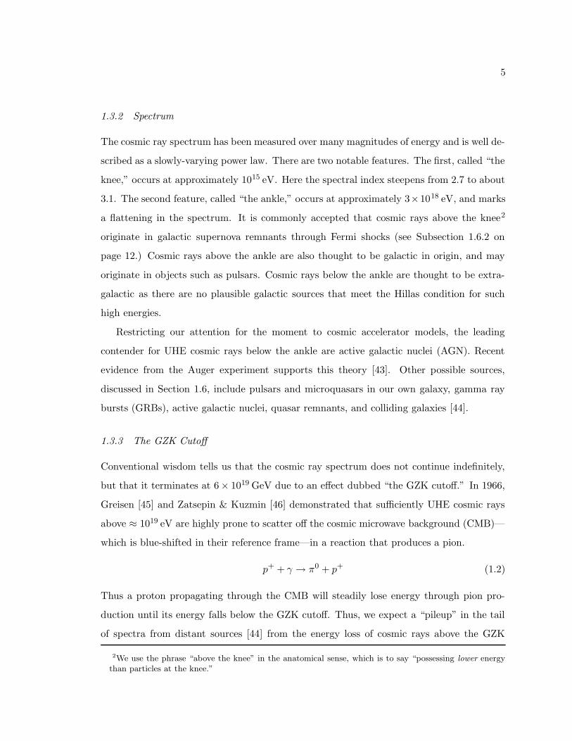
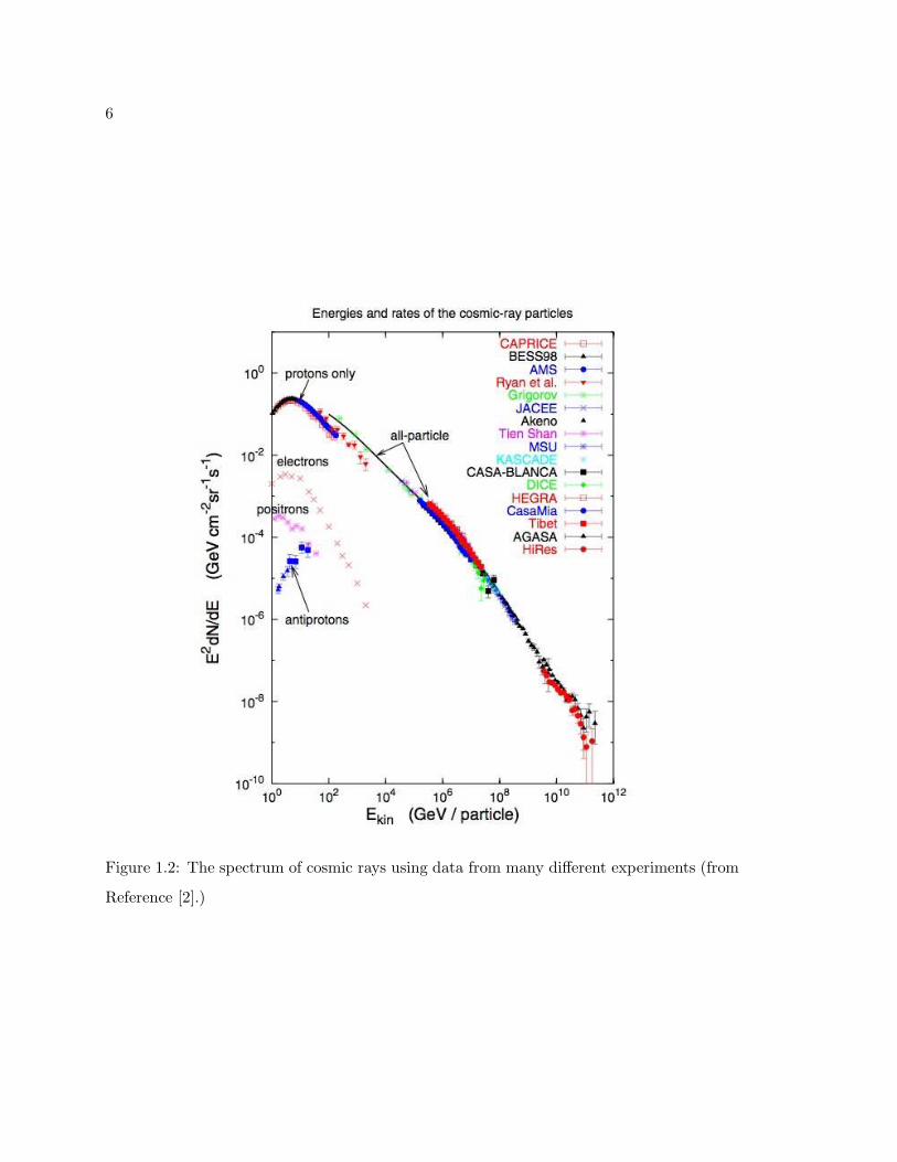
Figure 1.2: The spectrum of cosmic rays using data from many different experiments (from
Reference [2].)
7
cutoff. In order for cosmic rays in excess of the GZK cutoff to reach Earth, they would have
to be created by a nearby source within 50Mpc (163Mly).3 Thus, confirmation of cosmic
rays with energies in excess of the GZK cutoff may necessitate models more exotic than the
cosmic accelerator, such as those discussed in Section 1.5.
Observational evidence of the GZK cutoff is so far inconclusive, but it can be fairly
said that there is presently more and better evidence for the existence of the cutoff than
there is against it. The AGASA experiment has observed nine events with energy above
4 × 10¹⁹ eV, some of which are in apparent violation of the GZK cutoff [47]. Three other
experiments (with a combined exposure three times that of AGASA,) however, observe
GZK suppression, including HiRes [48], Fly’s Eye [49], and Yakutsk [50]. In an attempt
to reconcile this discrepancy, Bahcall and Waxman have argued that the AGASA anomaly
can be explained by supposing that the AGASA energy calibration is systematically high
by 11% [51]. Early results from the Auger experiment also appear to be consistent with
GZK suppression [43].
1.3.4 Composition
The composition of UHE cosmic rays is also a matter of some controversy. Cosmic ray
composition is determined by using MC to correlate the atomic number of the primary
particle with the atmospheric depth at which its shower of secondary particles reaches
maximum size and the proportion of muons at ground level. As of yet it has been difficult to
achieve agreement between different MC algorithms as well as between different experiments.
Recent data from the Auger experiment [52] favors a mixed composition at and above the
ankle, composed of significant fractions of protons as well as heavier elements. HiRes, on the
other hand, favors a spectrum that is increasingly dominated by protons at higher energies
[53]. The fraction of gamma rays in the UHE cosmic ray flux are constrained by Auger to
be less than 2% [54].4
3For comparison, the Milky Way is ≈ 0.1 Mly = 0.03 Mpc in diameter, and Andromeda, the nearest spiralgalaxy, is ≈ 2.5 Mly = 0.8 Mpc away.
4Gamma rays, at these energies scatter off the CMB (by pair production,) so the presence of gammarays in the UHE cosmic ray flux would be strong evidence for the existence of a nearby exotic source.Topological defects and Z-bursts, in particular, both predict large fluxes of photons.
8
1.3.5 Arrival Directions
By studying the arrival direction of the highest energy cosmic rays, we might hope to infer
their place of origin. This project is complicated by the fact that charged cosmic rays are
deflected by magnetic fields. If the coherence length (lc) of the intervening magnetic field
is small compared to the distance to the source (r), the deflection angle (αrms) can be
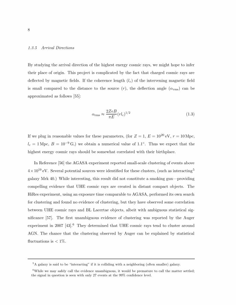
approximated as follows [55]:
αrms ≈2ZeB
πE(rlc)
1/2 (1.3)
If we plug in reasonable values for these parameters, (for Z = 1, E = 1020 eV, r = 10Mpc,
lc = 1Mpc, B = 10−9 G,) we obtain a numerical value of 1.1. Thus we expect that the
highest energy cosmic rays should be somewhat correlated with their birthplace.
In Reference [56] the AGASA experiment reported small-scale clustering of events above
4×10¹⁹ eV. Several potential sources were identified for these clusters, (such as interacting5
galaxy Mrk 40.) While interesting, this result did not constitute a smoking gun—providing
compelling evidence that UHE cosmic rays are created in distant compact objects. The
HiRes experiment, using an exposure time comparable to AGASA, performed its own search
for clustering and found no evidence of clustering, but they have observed some correlation
between UHE cosmic rays and BL Lacertae objects, albeit with ambiguous statistical sig-
nificance [57]. The first unambiguous evidence of clustering was reported by the Auger
experiment in 2007 [43].6 They determined that UHE cosmic rays tend to cluster around
AGN. The chance that the clustering observed by Auger can be explained by statistical
fluctuations is < 1%.
5A galaxy is said to be “interacting” if it is colliding with a neighboring (often smaller) galaxy.
6While we may safely call the evidence unambiguous, it would be premature to call the matter settled;the signal in question is seen with only 27 events at the 99% confidence level.
9
1.4 Cosmic Rays and Neutrinos: The Waxman-Bahcall Limit
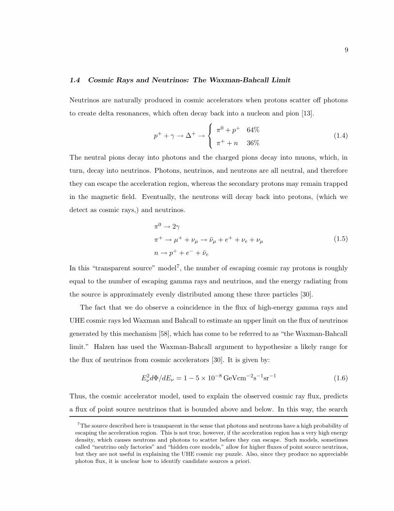
Neutrinos are naturally produced in cosmic accelerators when protons scatter off photons
to create delta resonances, which often decay back into a nucleon and pion [13].
p+ + γ → ∆+ →
π0 + p+ 64%
π+ + n 36%(1.4)
The neutral pions decay into photons and the charged pions decay into muons, which, in
turn, decay into neutrinos. Photons, neutrinos, and neutrons are all neutral, and therefore
they can escape the acceleration region, whereas the secondary protons may remain trapped
in the magnetic field. Eventually, the neutrons will decay back into protons, (which we
detect as cosmic rays,) and neutrinos.
π0 → 2γ
π+ → µ+ + νµ → νµ + e+ + νe + νµ
n→ p+ + e− + νe
(1.5)
In this “transparent source” model7, the number of escaping cosmic ray protons is roughly
equal to the number of escaping gamma rays and neutrinos, and the energy radiating from
the source is approximately evenly distributed among these three particles [30].
The fact that we do observe a coincidence in the flux of high-energy gamma rays and
UHE cosmic rays led Waxman and Bahcall to estimate an upper limit on the flux of neutrinos
generated by this mechanism [58], which has come to be referred to as “the Waxman-Bahcall
limit.” Halzen has used the Waxman-Bahcall argument to hypothesize a likely range for
the flux of neutrinos from cosmic accelerators [30]. It is given by:
E2νdΦ/dEν = 1 − 5 × 10⁻⁸ GeVcm−2s−1sr−1 (1.6)
Thus, the cosmic accelerator model, used to explain the observed cosmic ray flux, predicts
a flux of point source neutrinos that is bounded above and below. In this way, the search
7The source described here is transparent in the sense that photons and neutrons have a high probability ofescaping the acceleration region. This is not true, however, if the acceleration region has a very high energydensity, which causes neutrons and photons to scatter before they can escape. Such models, sometimescalled “neutrino only factories” and “hidden core models,” allow for higher fluxes of point source neutrinos,but they are not useful in explaining the UHE cosmic ray puzzle. Also, since they produce no appreciablephoton flux, it is unclear how to identify candidate sources a priori.
10
for neutrino point sources is intimately related to recent developments in the study of UHE
cosmic rays. The recent discovery by Auger of a correlation between UHE cosmic rays and
AGN is just the latest exciting piece in the puzzle of UHE astronomy.
1.5 Top-Down Versus Bottom-Up
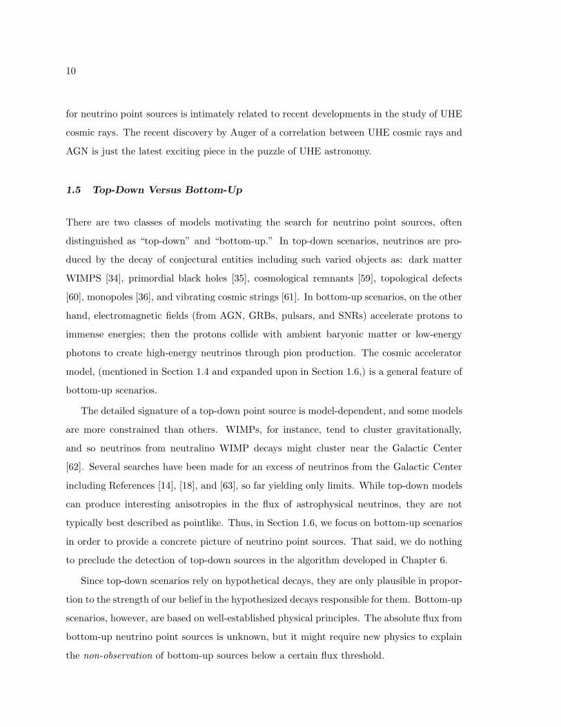
There are two classes of models motivating the search for neutrino point sources, often
distinguished as “top-down” and “bottom-up.” In top-down scenarios, neutrinos are pro-
duced by the decay of conjectural entities including such varied objects as: dark matter
WIMPS [34], primordial black holes [35], cosmological remnants [59], topological defects
[60], monopoles [36], and vibrating cosmic strings [61]. In bottom-up scenarios, on the other
hand, electromagnetic fields (from AGN, GRBs, pulsars, and SNRs) accelerate protons to
immense energies; then the protons collide with ambient baryonic matter or low-energy
photons to create high-energy neutrinos through pion production. The cosmic accelerator
model, (mentioned in Section 1.4 and expanded upon in Section 1.6,) is a general feature of
bottom-up scenarios.
The detailed signature of a top-down point source is model-dependent, and some models
are more constrained than others. WIMPs, for instance, tend to cluster gravitationally,
and so neutrinos from neutralino WIMP decays might cluster near the Galactic Center
[62]. Several searches have been made for an excess of neutrinos from the Galactic Center
including References [14], [18], and [63], so far yielding only limits. While top-down models
can produce interesting anisotropies in the flux of astrophysical neutrinos, they are not
typically best described as pointlike. Thus, in Section 1.6, we focus on bottom-up scenarios
in order to provide a concrete picture of neutrino point sources. That said, we do nothing
to preclude the detection of top-down sources in the algorithm developed in Chapter 6.
Since top-down scenarios rely on hypothetical decays, they are only plausible in propor-
tion to the strength of our belief in the hypothesized decays responsible for them. Bottom-up
scenarios, however, are based on well-established physical principles. The absolute flux from
bottom-up neutrino point sources is unknown, but it might require new physics to explain
the non-observation of bottom-up sources below a certain flux threshold.
11
1.6 Modeling Cosmic Accelerators
1.6.1 Direct and Statistical Acceleration
Broadly speaking, two mechanisms have have been proposed to explain how cosmic accel-
erators impart such high energies to UHE cosmic rays. In one mechanism, called “direct
acceleration,” particles are accelerated by an extended electric field, which is presumed
to arise from a rapidly rotating magnetized object. In the other model, (referred to by
a variety of names including “statistical acceleration,” “stochastic acceleration,” “Fermi
acceleration,” and “acceleration by shocks,”) particles are accelerated by repeated interac-
tions with magnetic fluctuations on the cusp of an out-of-equilibrium shock front created
by cosmic explosions, jets, or winds.
Statistical acceleration has the advantage that it naturally produces the dΦ/dE ∝ E−γ
power law spectrum that characterizes the cosmic ray spectrum, but it is hard to see how
to accomplish this with a direct acceleration model [1]. Another difficulty for direct accel-
eration models is that such strong extended electromagnetic fields are typically associated
with very high energy densities, which can cause energy loss at a rate that overcomes the
energy gained through acceleration. Statistical acceleration models are not free of technical
difficulties either, however; it is difficult to explain, for instance, how statistical acceleration
can accelerate particles above the knee [64]. The two mechanisms are not mutually exclusive
and they often occur in the same objects. For example, the super-massive, spinning, mag-
netic black holes that characterize AGN may be able to produce EMFs capable of immense
direct acceleration, while the jets of relativistic matter spewed from the AGN likely produce
acceleration by shocks [64].
Acceleration mechanisms can alternatively be classified as: shock acceleration, unipo-
lar induction, and magnetic flares, as in Reference [64]. Unipolar induction corresponds
to direct acceleration (from spinning magnetized objects,) and magnetic flares refer to the
sudden realignments of large-scale magnetic fields, which can create large EMFs (direct
acceleration) and shocks (statistical acceleration.) A prototypical example of flare accel-
eration occurs in our own sun, where electrons can be accelerated to energies in excess
of 1 MeV. Solar flares produce only modest accelerations, but flares from young, spinning
12
neutron stars with large magnetic fields (10-100 GT) called “magnetars” can produce po-
tential differences on the order of 1019 V, which makes them candidates for UHE cosmic
ray production. In Table 1.1 on the facing page, we document the most promising cosmic
accelerator scenarios and their mechanisms for acceleration.8 Each scenario is discussed in
greater detail in Subsection 1.7 on page 18.
1.6.2 Shocks
As many point source scenarios invoke the physics of shocks, it is worth exploring this
subject in more detail. Our goal is not an exhaustive treatment, but rather a qualitative
description of shockwaves. We begin by postulating the existence of some driving force,
which creates a jet, wind, or explosion of charged particles. In practice, the driving force is
often a black hole, supernova, or pulsar. Relevant examples of jets and wind are respectively
the jets associated with black hole accretion and the wind associated with rapidly spinning
neutron stars. In the discussion that follows, we assume the charged particles, (which we
can take to be protons,) will ultimately create neutrinos through pion production, and that
furthermore, the neutrinos will have a similar spectral shape to the protons that create
them.
The driving force creates a region called the “upstream” region where particles are
characterized by a velocity β1. The upstream region is taken to be next to a “downstream”
region of surrounding matter characterized by a typical velocity β2 < β1. The two regions
meet at a boundary called the “shock front,” (see Figure 1.3 on page 14.) In this discussion,
the shock front is taken to be stationary, and we measure the velocities β1 and β2 from the
“shock frame.”
By requiring the conservation of particle density, energy, and momentum at the shock
front, we obtain the so-called relativistic shock jump conditions [66].
Γ1β1n1 = Γ2β2n2
Γ21β1(ε1 + p1) = Γ2
2β2(ε2 + p2)
Γ21β
21(ε1 + p1) + p1 = Γ2
2β22(ε2 + p2) + p2
(1.7)
8We omit discussion of neutrinos from galactic clusters since it has been shown that the expected fluxfrom galaxy clusters is far smaller than other more promising models Reference [65].
13
Table 1.1: Key properties of proposed cosmic accelerator sources. (Quasar remnants, dis-
cussed in Subsection 1.7.7 on page 28, are not good neutrino point source candidates, though
they are potential cosmic accelerators.)
cosmic accelerator source proximity mechanism
magnetars: (also referred to as “soft gamma
repeaters” and “anomalous X-ray pulsars” de-
pending on their optical properties); young
pulsars with large magnetic fields
galactic flares
plerions: (also called “pulsar wind nebu-
lae”); old pulsars embedded in synchrotron
nebulae
galactic induction
SNRs: supernovae shockwaves colliding with
surrounding gas
galactic shocks
microquasars: (also called “radio-jet X-
ray binaries”); small black holes devouring a
neighboring star
galactic shocks, induction, flares
AGN: (called “blazars” when their jets are
pointed towards Earth); super-massive black
holes at the center of some galaxies
extragalactic shocks, induction
GRBs: thought to originate from the col-
lapse of high-mass stars
extragalactic shocks
quasar remnants: (also called “quiet black
holes” and “dormant AGN”) at the center of
nearby galaxies
extragalactic induction
14
drivingforce
upstream downstream
β1 β2
shock front
Figure 1.3: A pictorial representation of a shock front.
Γ, n, ε, and p are respectively the Lorentz factor, particle density, energy density, and
pressure (all measured in the frame denoted by their subscript.) We have assumed a small
magnetic field for the sake of simplicity.9
As the shockwave propagates through space, particles can diffuse across the shock front
between the upstream and downstream regions. In either region, they will scatter on mag-
netic irregularities, (called Alfven waves,) which are approximated to be at rest with respect
to the fluid in their respective regions. Since the irregularities are at rest, the energy of the
scattered particle is unchanged, but its momentum vector will, in general, change orienta-
tion. Consider a particle that diffuses across the shock front from the upstream region to
the downstream region, scatters on a magnetic irregularity, and diffuses back (as illustrated
in Figure 1.4 on the next page.) Since the particle’s momentum vector changes orientation
after scattering, (and angles are not invariant under Lorentz transformations,) its energy
will change depending on the crossing angles before and after scattering, as described in
Equation 1.8.10
Ef
Ei= Γ2
rel[1 − βrel cos(θ→d)][1 + βrel cos(θ′→u)] (1.8)
Ef and Ei are the final and initial energy of the particle. βrel is the relative velocity of
the upstream and downstream regions, and Γrel is the corresponding Lorentz factor. θ→d is
the crossing angle between the particle’s momentum vector and the shock front normal as
9Magnetized shocks are parameterized by the magnetization parameter, σ ≡ B21/4π(ε1 + p1), which we
assume to be close to unity in our approximation. For a treatment of magnetized shocks, see Reference [67].
10As a sanity check, we note that the special case of θ→d = θ′→u = 0 yields the expected result that
Ef = Ei.
15
upstream downstream
shock front
θ->d
θ’->u
βsh
Figure 1.4: A particle diffusing across the shock front and back.
a particle diffuses downstream; θ′→u is the crossing angle between the particle’s momentum
vector and the shock front normal as a particle diffuses back upstream. Primed quantities
are measured downstream, unprimed upstream.
If the particle crosses and recrosses the shock front, we can compute the average energy
gained by integrating over the crossing angles. For non-relativistic shocks, we can assume
that the distribution of angles is nearly isotropic, and it can be shown [66] that the average
ratio of final to initial energy is given by Equation 1.9.
〈Ef/Ei〉 ≈ 1 + (4/3)βrel (1.9)
Equation 1.9 does not hold for highly relativistic shocks—the crossing angles for ultra-
relativistic shocks are highly anisotropic—but it still may be said that the average energy
gained on one crossing-recrossing of the shock front is on the order of the particle’s existing
energy [64].
Thus, particles near the shock front will tend to gain energy with each crossing until
they are able to escape from the shock. The escape probability is given by the ratio of flux
far downstream to the flux of particles through the shock front.
Pescape = Φdownstream/Φshock
For non-relativistic shocks, the escape probability, determined in Reference [66], is given
by Pescape = 4β2. Simulations of relativistic shocks produce a power law spectrum among
shocked particles (as in Equation 1.10,) which is largely robust to details about the extent
16
to which the particles are relativistic.
dN/dE ∝ E−γ (1.10)
The spectral index γ is close to 2 for a wide range of models [66]. Encouragingly, this agrees
with observations of γ = 2.2− 2.3 for electromagnetic radiation from GRBs and SNRs such
as GRB 970508 [66]. The power law structure is indicative of scale invariance in the shock
process.
The power law spectrum, however, does not continue to arbitrarily high energies. Even-
tually, it is cut off by the fact that shockwaves exist for a finite time. We can calculate an
approximate maximum shock energy by examining the time it takes for a particle of energy
E and charge q to increase its energy by an amount on the order of E in the presence
of a shock wave with a gamma factor of Γsh and a typical magnetic field of B1, given in
Equation 1.11.
tacc ≈ E/(qΓshB1) (1.11)
We require that the acceleration time be less than the duration of the shocks, tsh = Rsh,
where Rsh is the blast radius and we are working in natural units. We thus obtain a
maximum energy given by Equation 1.12.
Emax ≈ qB1ΓshRsh (1.12)
Equation 1.12 is similar to the familiar expression for the energy of a charged particle moving
in a uniform magnetic field, except for the gamma factor, Γsh, which reflects the relativistic
and stochastic nature of shocks.
As shock acceleration occurs on the boundary between two regions not in thermal equilib-
rium, shocks are necessarily a non-thermal process. They convert ambient electromagnetic
energy into the kinetic energy of shocked particles, which exhibit a power law spectrum
with a spectral index of γ ≈ 2. Particles reach a maximum energy, which is constrained
by the local magnetic field, the shock radius, and the gamma factor associated with the
shock. The description here can be extended to include strong magnetic fields and more
sophisticated fluid mechanics, such as turbulence, but the big picture remains the same.
17
1.6.3 Galactic and Extragalactic Sources
In Table 1.1 on page 13, we list four galactic scenarios and three extragalactic scenarios
for the bottom-up acceleration of UHE cosmic rays. (Six of these seven scenarios are also
promising models of neutrino point sources.) There are several points worth making with
regard to this dichotomy. First, it is important to note that there is evidence of both galactic
and extragalactic sources in the form of the broken power law described in Subsection 1.3.2.
Null results for searches for large-scale anisotropy of UHE cosmic rays [56], as well as data
linking UHE cosmic rays to AGN [43], suggest that the highest energy cosmic rays are
extragalactic in origin. Second, attempts to link high-energy cosmic rays to galactic sources
are frustrated by the fact that cosmic rays from galactic sources are more strongly affected by
magnetic fields than extragalactic UHE cosmic rays. Neutrinos, therefore, provide us with
a unique opportunity to resolve galactic sources. Third, galactic sources tend to cluster
near the Galactic Center [33]. Since neutrino detectors rely on upward-going muons to
identify neutrino events in excess of 1GeV, (see Chapter 5,) Super-Kamiokande, located in
the northern hemisphere, is exposed to sources in the southern sky. This provides us with a
distinct advantage over IceCube, which, situated near the South Pole, is insensitive to the
Galactic Center.
Fourth, if we naively interpret the cosmic ray spectrum as an indicator of the neutrino
point source spectrum, we conclude that the flux from galactic point sources (below the
knee) is higher than the flux from extragalactic point sources (above the knee.) We might,
therefore, expect to detect galactic neutrino point sources before extragalactic point sources.
Reality is complicated by the fact that the signal from neutrino point sources competes
for detection with the steeply falling atmospheric neutrino background spectrum created
from cosmic rays interacting with the atmosphere, (see Chapter 2.) It may turn out that
UHE neutrinos from extragalactic sources have a higher signal to noise ratio (compared to
neutrinos from galactic sources,) despite their small absolute flux.
18
1.7 Scenarios for Cosmic Acceleration
1.7.1 Magnetars
Magnetars are young pulsars with strong magnetic fields on the order of 1015 G and periods
on the order of seconds. A typical magnetar spins at a relatively steady rate for the first few
hundred years of its life. By the time a magnetar becomes thousands of years old, it will
have begun to convert some of its immense rotational energy into electromagnetic radiation.
The electromagnetic slowdown of a magnetar is observed in the optical spectrum as irregular
bursts of low-energy gamma rays and X-rays, which has led to the categorization of some
magnetars as soft gamma repeaters (SGRs) and anomalous X-ray pulsars (AXPs).
Young magnetars are interesting candidates for the production of point source neutrinos
(and high-energy cosmic rays) since the power produced during their spin-down phase can
exceed the magnetic power produced later in the magnetar’s life (when it has become an
SGR/AXP.) Their magnetic power, meanwhile, provides a high density of photons near the
magnetar’s surface, which provide a target for accelerated protons from which to create
neutrinos through pion production [20].
In order for a magnetar to produce copious neutrinos, its spin must have a significant
component antiparallel to its magnetic field. If this is the case, and it likely is roughly half of
the time [20], the spin-induced electric field will accelerate (positively charged) protons away
from the surface where they can interact with photons near the polar caps to produce delta
resonances, which ultimately decay into neutrinos as described in Equations 1.4 and 1.5 on
page 9. By comparing the threshold energy above which protons create neutrinos via delta
resonances with the maximum energy of accelerated protons—(a function of magnetar ra-
dius, magnetic field (B), and period (P ))—a range of parameter space in the log(B)-log(P )
plane can be determined wherein magnetars have the potential to be neutrino-loud [20].
The neutrino-loud region has been nicknamed the “neutrino death valley,” and it is most
likely to yield neutrino point sources in the range of P ≈ 4 s and B ≈ 1015 G.
Magnetars tend to produce highly beamed bursts covering on average 0.1 radians of
solid angle (0.8% of the unit sphere.) This is a mixed blessing from the perspective of
experimentalists hoping to detect magnetar neutrinos. If the magnetar beam happens to be
19
Table 1.2: Magnetar point source candidates identified in Reference [20]. dN 2µ/dAdt is
the expected flux of upward-going muons (for Eν > 1TeV) given favorable conditions.
Equatorial coordinates come from Reference [21].
candidate distance (kpc) d2Nµ/dAdt (km−2yr−1) (ra,dec)
SGR 1900+14 3.0-9.0 1.5-13 (286.8,+9.3)
SGR 0526-66 ≈ 50 ≈ 0.003 (81.5,−66.0)
1E 1048.1-5937 2.5-2.8 0.5-0.7 (162.5,−59.9)
SGR 1806-20 13.0-16.0 0.01-0.02 (272.2,−20.4)
pointing towards Earth, the experimentalist is the recipient of a signal that is many times
magnified from what it would be if the neutrinos were emitted isotropically. The other side
of this coin is that it is improbable that the magnetar beam is pointed at Earth.
There are currently fourteen confirmed magnetars [68]. Four have been identified as
candidate sources that may be detectable on Earth [20]. We list these candidate magnetars
in Table 1.2 along with upmu flux calculated in Reference [20] assuming favorable condi-
tions. Luckily, all four fall inside Super-Kamiokande’s sensitive region (dec< +54). Upmu
flux is calculated for neutrino energies in excess of 1TeV to illustrate the possible signals
at kilometer-scale detectors, which have relatively high energy thresholds. The upmu en-
ergy threshold at Super-Kamiokande is just 1.6GeV, so we are sensitive to a higher flux
than quoted in Table 1.2. (Of course, the background from atmospheric neutrinos rapidly
increases at lower energies.)
1.7.2 Plerions
Plerions, or pulsar wind nebulae (PWN), are nebulae characterized by an embedded pulsar.
They are thought to be created from supernovae, but not every plerion has a (visible)
supernova remnant because it is not always possible to observe the requisite blast wave.11
11In some of the literature, plerions are categorically considered to be SNR, (whether or not there is anobserved blast wave,) because it is frequently presumed that all plerions are created by supernovae.
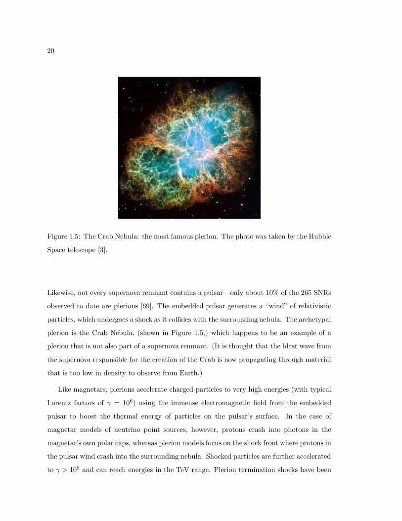
20
Figure 1.5: The Crab Nebula: the most famous plerion. The photo was taken by the Hubble
Space telescope [3].
Likewise, not every supernova remnant contains a pulsar—only about 10% of the 265 SNRs
observed to date are plerions [69]. The embedded pulsar generates a “wind” of relativistic
particles, which undergoes a shock as it collides with the surrounding nebula. The archetypal
plerion is the Crab Nebula, (shown in Figure 1.5,) which happens to be an example of a
plerion that is not also part of a supernova remnant. (It is thought that the blast wave from
the supernova responsible for the creation of the Crab is now propagating through material
that is too low in density to observe from Earth.)
Like magnetars, plerions accelerate charged particles to very high energies (with typical
Lorentz factors of γ = 106) using the immense electromagnetic field from the embedded
pulsar to boost the thermal energy of particles on the pulsar’s surface. In the case of
magnetar models of neutrino point sources, however, protons crash into photons in the
magnetar’s own polar caps, whereas plerion models focus on the shock front where protons in
the pulsar wind crash into the surrounding nebula. Shocked particles are further accelerated
to γ > 109 and can reach energies in the TeV range. Plerion termination shocks have been
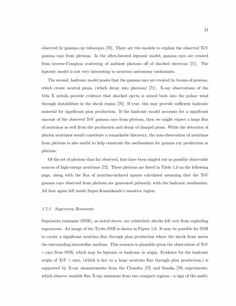
21
observed by gamma ray telescopes [70]. There are two models to explain the observed TeV
gamma rays from plerions. In the often-favored leptonic model, gamma rays are created
from inverse-Compton scattering of ambient photons off of shocked electrons [71]. The
leptonic model is not very interesting to neutrino astronomy enthusiasts.
The second, hadronic model posits that the gamma rays are created by beams of protons,
which create neutral pions, (which decay into photons) [71]. X-ray observations of the
Vela X nebula provide evidence that shocked ejecta is mixed back into the pulsar wind
through instabilities in the shock region [70]. If true, this may provide sufficient hadronic
material for significant pion production. If the hadronic model accounts for a significant
amount of the observed TeV gamma rays from plerions, then we might expect a large flux
of neutrinos as well from the production and decay of charged pions. While the detection of
plerion neutrinos would constitute a remarkable discovery, the non-observation of neutrinos
from plerions is also useful to help constrain the mechanisms for gamma ray production in
plerions.
Of the set of plerions thus far observed, four have been singled out as possibly observable
sources of high-energy neutrinos [72]. These plerions are listed in Table 1.3 on the following
page, along with the flux of neutrino-induced upmus calculated assuming that the TeV
gamma rays observed from plerions are generated primarily with the hadronic mechanism.
All four again fall inside Super-Kamiokande’s sensitive region.
1.7.3 Supernova Remnants
Supernova remnants (SNR), as noted above, are relativistic shocks left over from exploding
supernovae. An image of the Tycho SNR is shown in Figure 1.6. It may be possible for SNR
to create a significant neutrino flux through pion production where the shock front meets
the surrounding interstellar medium. This scenario is plausible given the observation of TeV
γ rays from SNR, which may be leptonic or hadronic in origin. Evidence for the hadronic
origin of TeV γ rays, (which is key to a large neutrino flux through pion production,) is
supported by X-ray measurements from the Chandra [75] and Suzaka [76] experiments,
which observe variable flux X-ray emissions from two compact regions—a sign of the multi-
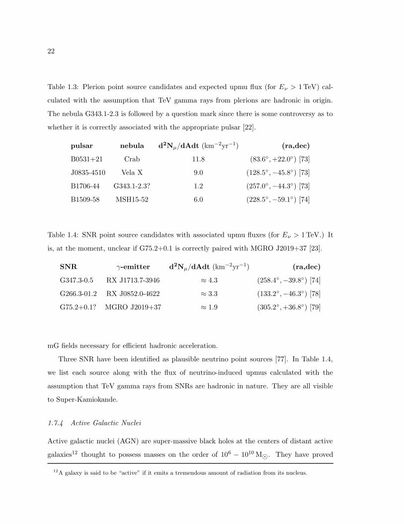
22
Table 1.3: Plerion point source candidates and expected upmu flux (for Eν > 1TeV) cal-
culated with the assumption that TeV gamma rays from plerions are hadronic in origin.
The nebula G343.1-2.3 is followed by a question mark since there is some controversy as to
whether it is correctly associated with the appropriate pulsar [22].
pulsar nebula d2Nµ/dAdt (km−2yr−1) (ra,dec)
B0531+21 Crab 11.8 (83.6,+22.0) [73]
J0835-4510 Vela X 9.0 (128.5,−45.8) [73]
B1706-44 G343.1-2.3? 1.2 (257.0,−44.3) [73]
B1509-58 MSH15-52 6.0 (228.5,−59.1) [74]
Table 1.4: SNR point source candidates with associated upmu fluxes (for Eν > 1TeV.) It
is, at the moment, unclear if G75.2+0.1 is correctly paired with MGRO J2019+37 [23].
SNR γ-emitter d2Nµ/dAdt (km−2yr−1) (ra,dec)
G347.3-0.5 RX J1713.7-3946 ≈ 4.3 (258.4,−39.8) [74]
G266.3-01.2 RX J0852.0-4622 ≈ 3.3 (133.2,−46.3) [78]
G75.2+0.1? MGRO J2019+37 ≈ 1.9 (305.2,+36.8) [79]
mG fields necessary for efficient hadronic acceleration.
Three SNR have been identified as plausible neutrino point sources [77]. In Table 1.4,
we list each source along with the flux of neutrino-induced upmus calculated with the
assumption that TeV gamma rays from SNRs are hadronic in nature. They are all visible
to Super-Kamiokande.
1.7.4 Active Galactic Nuclei
Active galactic nuclei (AGN) are super-massive black holes at the centers of distant active
galaxies12 thought to possess masses on the order of 106 − 1010 M. They have proved
12A galaxy is said to be “active” if it emits a tremendous amount of radiation from its nucleus.
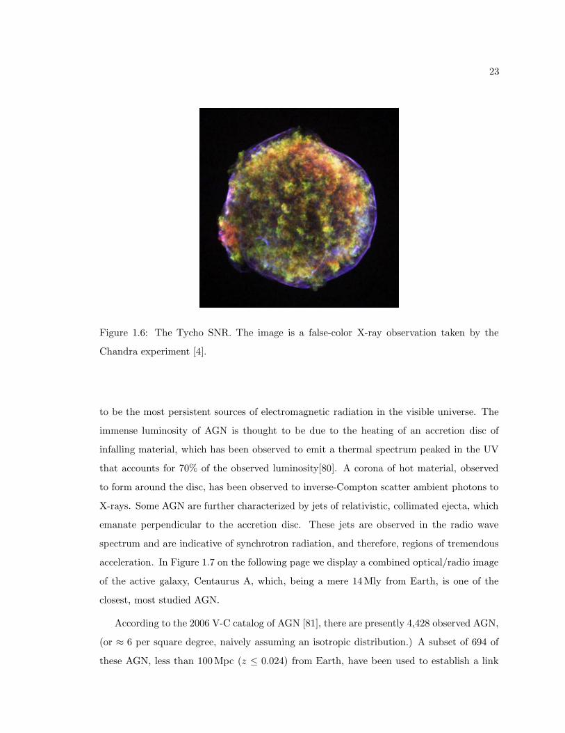
23
Figure 1.6: The Tycho SNR. The image is a false-color X-ray observation taken by the
Chandra experiment [4].
to be the most persistent sources of electromagnetic radiation in the visible universe. The
immense luminosity of AGN is thought to be due to the heating of an accretion disc of
infalling material, which has been observed to emit a thermal spectrum peaked in the UV
that accounts for 70% of the observed luminosity[80]. A corona of hot material, observed
to form around the disc, has been observed to inverse-Compton scatter ambient photons to
X-rays. Some AGN are further characterized by jets of relativistic, collimated ejecta, which
emanate perpendicular to the accretion disc. These jets are observed in the radio wave
spectrum and are indicative of synchrotron radiation, and therefore, regions of tremendous
acceleration. In Figure 1.7 on the following page we display a combined optical/radio image
of the active galaxy, Centaurus A, which, being a mere 14Mly from Earth, is one of the
closest, most studied AGN.
According to the 2006 V-C catalog of AGN [81], there are presently 4,428 observed AGN,
(or ≈ 6 per square degree, naively assuming an isotropic distribution.) A subset of 694 of
these AGN, less than 100Mpc (z ≤ 0.024) from Earth, have been used to establish a link
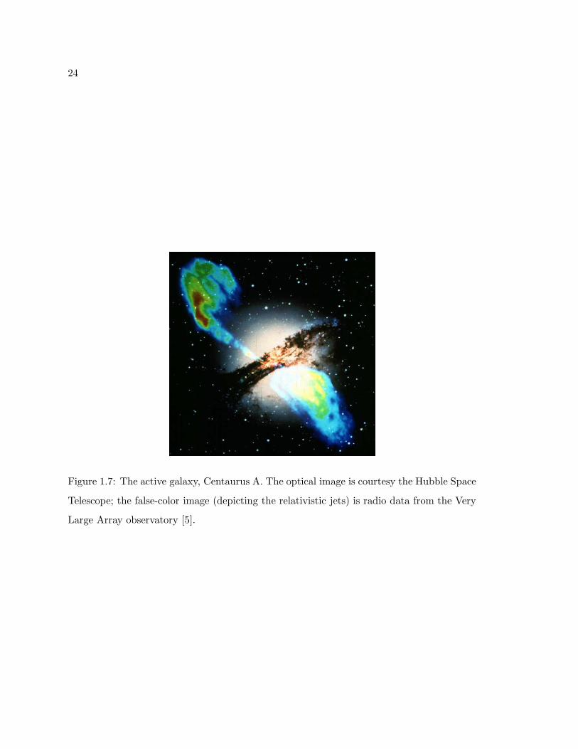
24
Figure 1.7: The active galaxy, Centaurus A. The optical image is courtesy the Hubble Space
Telescope; the false-color image (depicting the relativistic jets) is radio data from the Very
Large Array observatory [5].
25
between UHE cosmic rays and AGN [43]. There are certainly more AGN, hidden for the
moment behind the galactic plane. Also, it is likely that additional AGN not obscured by
the galactic plane await detection at distances greater than 100Mpc. It has been pointed
out that the detection of neutrinos from single distant AGN may be difficult in the presence
of a relatively large diffuse flux integrated over all AGN [82].
There are nine categories of AGN based on their electromagnetic observational charac-
teristics. The idiosyncratic classification of AGN relates to the orientation of the jets, the
relative strength of optical and radio emission, and other historically important features
used to categorize onetime disparate objects that came to be unified as AGN. Readers in-
terested in more details about the classification of AGN are referred to Reference [83]. The
different categories of AGN are:
• IR Astronomical Satellite (IRAS) blazars
• keV X-ray blazars
• GeV blazars
• unidentified GeV sources
• TeV blazars
• GHz Peaked Source (GPS) and Compact Steep Spectrum (CSS)
• FR-I radio galaxies
• FR-II radio galaxies
• radio-weak quasars
Neutrino production in AGN has been hypothesized to occur in the AGN core as well
as the termination shocks in the jets [82]. In either case protons are accelerated via Fermi
shocks, creating a dΦ/dE ∝ E−2 spectrum with a maximum energy near the GZK cutoff.
26
As always, pion production occurs through collisions with photons. At ≈ 30TeV, the
diffuse AGN neutrino flux is expected to become larger than the rapidly dropping flux of
atmospheric neutrinos [82].
1.7.5 Microquasars
Microquasars are binary systems in our own galaxy, which mimic some of the properties
and observational signatures of AGN. Like AGN, microquasars are thought to posses an
accretion disc. In the case of microquasars, the accretion disc is formed by the infall of
matter from a binary star into a black hole or neighboring neutron star. Also like AGN,
microquasars possess jets of ejected particles perpendicular to the accretion disc. Radio
and X-ray measurements of microquasar jets show the jets to be relativistic, creating shock
conditions, which may produce TeV energy neutrinos through the standard pion production
scenario described above [84]. Microquasars have been observed to exhibit flares, charac-
terized by increased X-ray luminosity, with timescales that can vary from minutes to days.
It is, presently, unknown whether these flares are associated with the ejection of plasma
or termination shocks in a quasisteady jet [84]. Perhaps the most famous microquasar is
Cygnus X-1, due to its role in the early debate on the existence of black holes.
In Reference [24], five microquasars are identified as possible point source candidates.
Two are considered optimal due to their steady, high, predicted fluxes, while the three
other microquasars suggested are of the “bursting” variety—characterized by flares—and
may thus require timing cuts to resolve. These microquasar point source candidates are
summarized in Table 1.5 on the next page.
1.7.6 Gamma Ray Bursts
Gamma ray bursts (GRBs) are extremely luminous events observed at high redshift, typi-
cally z > 1, which corresponds to 6Bly. During the duration of the blast, which typically
lasts seconds, but can range from milliseconds to minutes, the GRB is the most luminous
object in the visible universe. GRBs are thought to be caused by the dissipation of an
expanding fireball of ultrarelativistic particles (γ ≈ 100) created from the collapse of ex-
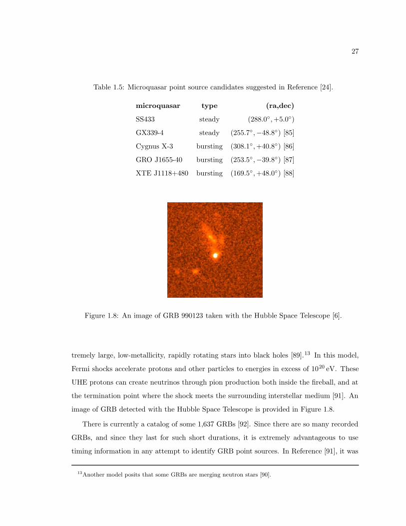
27
Table 1.5: Microquasar point source candidates suggested in Reference [24].
microquasar type (ra,dec)
SS433 steady (288.0,+5.0)
GX339-4 steady (255.7,−48.8) [85]
Cygnus X-3 bursting (308.1,+40.8) [86]
GRO J1655-40 bursting (253.5,−39.8) [87]
XTE J1118+480 bursting (169.5,+48.0) [88]
Figure 1.8: An image of GRB 990123 taken with the Hubble Space Telescope [6].
tremely large, low-metallicity, rapidly rotating stars into black holes [89].13 In this model,
Fermi shocks accelerate protons and other particles to energies in excess of 1020 eV. These
UHE protons can create neutrinos through pion production both inside the fireball, and at
the termination point where the shock meets the surrounding interstellar medium [91]. An
image of GRB detected with the Hubble Space Telescope is provided in Figure 1.8.
There is currently a catalog of some 1,637 GRBs [92]. Since there are so many recorded
GRBs, and since they last for such short durations, it is extremely advantageous to use
timing information in any attempt to identify GRB point sources. In Reference [91], it was
13Another model posits that some GRBs are merging neutron stars [90].
28
determined that GRBs should produce a flux of about 10-100 upmus per square kilometer
per year, (assuming the validity of the “fireball” model discussed above.) In fact, the ob-
servation of neutrinos from GRBs could be very useful as a test of the fireball model [91].
Another interesting (if perhaps fanciful) proposal is to use neutrinos from short-duration
GRBs to test both special relativity and the weak equivalence principle by comparing the
arrival times of massive neutrinos with massless gamma rays [91]. A study comparing
observed GRBs with neutrinos at Super-Kamiokande found no statistically significant cor-
relation between neutrinos and GRBs [93].14
1.7.7 Quasar Remnants
Extremely luminous AGN with ≥ 109 M (quasars) tend to be observed at very large
redshifts. Large redshifts, in turn, are associated with the early universe. Why then, one
might ask, is the present epoch devoid of quasars? It is presumed that quasar remnants
populate the centers of nearby galaxies [94]. In some models [95], these quasar remnants
have accreted all nearby gas and persist in nearly gas-free environments. They therefore
have no jets and are considerably less luminous than AGN. There may be as many as
≈ 40 quasar remnants within 50Mpc of Earth. Despite the low density of surrounding
gas, quasar remnants may still possess sufficient EMFs to accelerate individual particles to
energies near the GZK cutoff [94]. In this scenario, sometimes referred to “the Blandford-
Znajek mechanism” [96], supermassive spinning black holes create an enormous potential
difference by dragging magnetic field lines in the nearby warped space.
One advantage of the quasar remnant theory of UHE cosmic rays is that it can explain
apparent violations of the GZK cutoff, such as those seen by AGASA, since some quasar
remnants may be relatively close to Earth. A MC simulation of 37 nearby galaxies [97],
however, revealed that quasar remnants—if they are responsible for the bulk of observed
UHE cosmic rays—would produce significant anisotropies inconsistent with data. A more
pressing complaint from the standpoint of neutrino astronomy, however, is that quasar
remnants ought not to produce many neutrinos due to the low density of target material
14A study of the upmu dataset, in particular, used a 15 search cone and a conservative ±1,000 s timewindow to search for coincidences.
29
around them. Still, we include this mention of quasar remnants in our discussion of cosmic
accelerator models for the sake of completeness.
1.8 Related Searches and Experiments
1.8.1 Previous Searches by Super-Kamiokande
This study expands on four previous Super-Kamiokande studies related (at least indirectly)
to neutrino point sources. As discussed in Subsection 1.7.6 on page 26, a 2002 study [93]
determined no significant correlation between Super-Kamiokande neutrinos and observed
GRBs using data from SK-I. The study included an analysis of upmu events within a
±1000 s window of each cataloged GRB. It was additionally required that the upmu be
separated by < 15 from the GRB. In References [12] and [14], a high-energy subset of SK-
I upmus identified as showering (see Section 5.6 on page 108), were analyzed for pointlike
clustering. The authors employed Poisson statistics to determine the significance of possible
excess events in 3 and 4 half-angle search cones and found no evidence of neutrino point
sources at detectable levels.
In Reference [98], a search was performed for UHE neutrinos (in excess of 1 TeV) using
data from SK-I. The search yielded a single UHE neutrino, which was consistent with
expected background from atmospheric neutrinos. In Reference [99], a search for clustering
was performed using all upmus from the SK-I dataset. The author performed the test using
Poisson statistics to determine possible excess events in 4 × 4 and 3 × 3 bins. No excess
was detected.15
The analysis presented in this thesis differs significantly in several respects from previous
analyses.
• Combined analysis. This is the first point source study to expand the dataset to
include SK-II and SK-III.16
15In an unpublished study [100], a test was performed to measure deviations in the two point correlationfunction expected from atmospheric neutrino background. No statistically significant deviations weredetected.
16A degree of subtlety is required in order to take into account reduced detector resolution during theSK-II phase (see Chapter 6.)
30
• New likelihood technique. We develop and employ for the first time a likelihood
function, (described in great detail in Chapter 6,) which uses information such as the
detector’s point spread function to produce a “maximally sensitive result,” limited
only by the detector (as opposed to the algorithm.)
• Showering muons. This analysis is the first to integrate information about the
high-energy showering muon subsample into an analysis of the entire upmu dataset.
• Integrated flux limits. This analysis will provide the first Super-Kamiokande flux
limits integrated over the entire visible sky.
• Quasi-blind analysis. Unlike Reference [99], the analysis procedure is developed
entirely with MC.
• Point source MC This analysis is the first to utilize specially generated point source
MC to test the performance of the search algorithm.
• Special treatment of AGN and GRBs. We employ novel techniques to the special
cases of AGN and GRBs.
1.8.2 Point Source Searches with Other Experiments
The AMANDA-II experiment at the South Pole consists of strings of PMTs in polar
ice. At the time of their 2004 publication, AMANDA had a larger surface area than
Super-Kamiokande, but their minimum upmu energy is 10GeV in contrast with Super-
Kamiokande’s 1.6GeV. They are sensitive to neutrinos from the northern sky dec > 0,
whereas Super-Kamiokande is sensitive to neutrinos from −90 < dec+ < 54. In 2004 they
performed a binned search of the sky using 699 upward-going muons and optimized bins
ranging from 6 to 10 in size.17 They also looked for excesses of events from predetermined
galactic and extragalactic candidates (such as blazars and magnetars) in search cones of
unspecified radii. No evidence for point sources was discovered. A separate study [83] by
17The grid was shifted four times and averaged to address the issue of bin boundaries.
31
AMANDA-II, using the same dataset, implemented a source stacking scheme (discussed
briefly in Subsection 1.7.4 on page 22) to search for a correlation of neutrinos with AGN.
No evidence of this correlation was discovered.
The Baikal Neutrino Telescope is operated in Lake Baikal, Siberia at a depth
of 1.1 km. They are sensitive to UHE neutrinos. In a six-year study from 1998-2003,
they looked for excess neutrinos from predetermined candidate sources [101], though their
methodology is not immediately obvious. They found no evidence for excess neutrinos from
their predetermined sources.
The MACRO experiment, located in an underground mine in Gran Sasso, is a 77m
long box of scintillator, streamer tubes, and PMTs. In a 2001 publication [18], they per-
formed a search for the clustering of upmu events using 1, 3, and 5 cones and using
each of the 1,100 events as a search direction. They also performed the cone tests on a
catalog of predetermined candidates. No evidence was found of pointlike clustering. See
also Reference [102].
1.8.3 Radio-Neutrino Experiments
At least three experiments have used radio waves from UHE neutrino-induced electromag-
netic cascades to constrain the flux of UHE neutrinos: ANITA [103], FORTE [104], and
RICE [105]. These experiments are associated with neutrinos in the ≈ 1017−1020 eV range.
At these energies, the flux should be dominated by extragalactic sources, so any neutrinos
detected at this energy are attributable to distant sources. While the expected flux is low,
radio-neutrino experiments benefit from enormous effective areas. So far, however, these
experiments have yielded only limits.
1.8.4 Future Point Source Experiments
There are several notable experiments either in construction or proposal phases, that may
contribute to the search for neutrino point sources. In Section 1.2 on page 2, we discussed
the IceCube experiment, which will expand the AMANDA detector to a kilometer scale
detector. Extensive work has been compiled documenting the physics potential of IceCube

32
and other kilometer scale detectors proposed for the northern hemisphere [106], [26]. Large
neutrino detectors designed for long baseline neutrino beams and detection of the diffuse
supernova flux may also provide interesting observations of point sources [27], [28].
33
Chapter 2
ATMOSPHERIC NEUTRINOS AND THE EARTH SHADOW EFFECT
In Chapter 1, we discussed the motivation for a neutrino point source search. In Chap-
ters 3 and 5, we will describe how neutrinos are detected at Super-Kamiokande through
the observation of upward-going muons (upmus). We shall see that the only significant
background to a search for neutrino point sources at upmu energies (in excess of 1.6GeV)
is from atmospheric neutrinos created from the interactions of cosmic rays with the Earth’s
atmosphere. Therefore, it is necessary to carefully characterize the atmospheric neutrino
background if we hope to extract a signal above it, and that is the aim of the present
chapter. Our discussion of atmospheric neutrinos here will provide key ingredients in our
detector simulation described in Chapter 4.
2.1 From Cosmic Rays to Atmospheric Neutrinos
As discussed in Subsection 1.3.5 on page 8, the angular distribution of cosmic rays is very
nearly isotropic up to energies of 1019 eV, where there is some evidence of clustering in
the extragalactic plane. The highest energy upmus at Super-Kamiokande have energies
< 100TeV, and so we operate in an energy range well below the scale where clustering may
occur. The energy spectrum, described in Subsection 1.3.2 on page 5, is well described as
a broken power law spectrum, with a spectral index of γ = 2.7, over the relevant upmu
energy range. The composition of cosmic rays in our energy range, (see Subsection 1.3.4 on
page 7,) is ≈ 90% protons, ≈ 9% alpha particles, and ≈ 1% heavier nuclei [33].
When cosmic rays collide with the atmosphere, they produce hadronic showers, domi-
nated by pions up to 200GeV. Above 200GeV there is a contribution from kaons, and by
charmed mesons (D and ∆ particles) starting at 20TeV, depending on the zenith angle [33].
These mesons produce neutrinos by decaying into muons as in some examples included in
Table 2.1 along with the associated branching ratios and meson lifetimes.
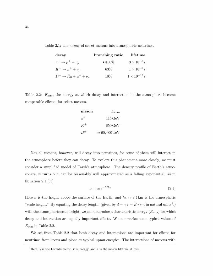
34
Table 2.1: The decay of select mesons into atmospheric neutrinos.
decay branching ratio lifetime
π+ → µ+ + νµ ≈100% 3 × 10⁻⁸ s
K+ → µ+ + νµ 63% 1 × 10⁻⁸ s
D+ → K0 + µ+ + νµ 10% 1 × 10⁻¹² s
Table 2.2: Eatm, the energy at which decay and interaction in the atmosphere become
comparable effects, for select mesons.
meson Eatm
π± 115GeV
K± 850GeV
D± ≈ 60, 000TeV
Not all mesons, however, will decay into neutrinos, for some of them will interact in
the atmosphere before they can decay. To explore this phenomena more closely, we must
consider a simplified model of Earth’s atmosphere. The density profile of Earth’s atmo-
sphere, it turns out, can be reasonably well approximated as a falling exponential, as in
Equation 2.1 [33].
ρ = ρ0 e−h/h0 (2.1)
Here h is the height above the surface of the Earth, and h0 ≈ 8.4 km is the atmospheric
“scale height.” By equating the decay length, (given by d = γ τ = E τ/m in natural units1,)
with the atmospheric scale height, we can determine a characteristic energy (Eatm) for which
decay and interaction are equally important effects. We summarize some typical values of
Eatm in Table 2.2.
We see from Table 2.2 that both decay and interactions are important for effects for
neutrinos from kaons and pions at typical upmu energies. The interactions of mesons with
1Here, γ is the Lorentz factor, E is energy, and τ is the meson lifetime at rest.
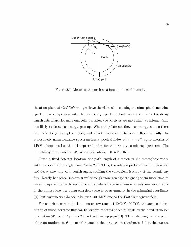
35
l[cos(θ1=0)]
l[cos(θ2=0)]
Super-Kamiokande
Earth
Atmosphere
θ2
Figure 2.1: Meson path length as a function of zenith angle.
the atmosphere at GeV-TeV energies have the effect of steepening the atmospheric neutrino
spectrum in comparison with the cosmic ray spectrum that created it. Since the decay
length gets longer for more energetic particles, the particles are more likely to interact (and
less likely to decay) as energy goes up. When they interact they lose energy, and so there
are fewer decays at high energies, and thus the spectrum steepens. Observationally, the
atmospheric muon neutrino spectrum has a spectral index of ≈ γ = 3.7 up to energies of
1PeV; about one less than the spectral index for the primary cosmic ray spectrum. The
uncertainty in γ is about 1.4% at energies above 100GeV [107].
Given a fixed detector location, the path length of a meson in the atmosphere varies
with the local zenith angle, (see Figure 2.1.) Thus, the relative probabilities of interaction
and decay also vary with zenith angle, spoiling the convenient isotropy of the cosmic ray
flux. Nearly horizontal mesons travel through more atmosphere giving them more time to
decay compared to nearly vertical mesons, which traverse a comparatively smaller distance
in the atmosphere. At upmu energies, there is no asymmetry in the azimuthal coordinate
(φ), but asymmetries do occur below ≈ 400MeV due to the Earth’s magnetic field.
For neutrino energies in the upmu energy range of 10GeV-100TeV, the angular distri-
bution of muon neutrino flux can be written in terms of zenith angle at the point of meson
production (θ∗) as in Equation 2.2 on the following page [33]. The zenith angle at the point
of meson production, θ∗, is not the same as the local zenith coordinate, θ, but the two are
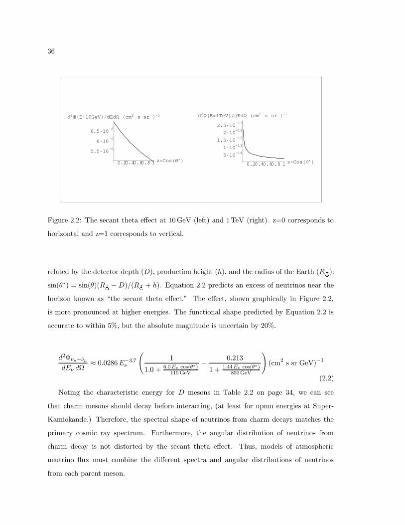
36
0.20.40.60.8 1 z=CosHΘ*L5.5·10-6
6·10-6
6.5·10-6
d2FHE=10GeVLdEdW Hcm2 s sr L-1
0.20.40.60.8 1 z=CosHΘ*L5·10-141·10-13
1.5·10-132·10-13
2.5·10-13
d2FHE=1TeVLdEdW Hcm2 s sr L-1
Figure 2.2: The secant theta effect at 10GeV (left) and 1TeV (right). z=0 corresponds to
horizontal and z=1 corresponds to vertical.
related by the detector depth (D), production height (h), and the radius of the Earth (R ):
sin(θ∗) = sin(θ)(R −D)/(R + h). Equation 2.2 predicts an excess of neutrinos near the
horizon known as “the secant theta effect.” The effect, shown graphically in Figure 2.2,
is more pronounced at higher energies. The functional shape predicted by Equation 2.2 is
accurate to within 5%, but the absolute magnitude is uncertain by 20%.
d2Φνµ+νµ
dEν dΩ≈ 0.0286E−3.7
ν
(
1
1.0 + 6.0 Eν cos(θ∗)115 GeV
+0.213
1 + 1.44 Eν cos(θ∗)850 GeV
)
(cm2 s sr GeV)−1
(2.2)
Noting the characteristic energy for D mesons in Table 2.2 on page 34, we can see
that charm mesons should decay before interacting, (at least for upmu energies at Super-
Kamiokande.) Therefore, the spectral shape of neutrinos from charm decays matches the
primary cosmic ray spectrum. Furthermore, the angular distribution of neutrinos from
charm decay is not distorted by the secant theta effect. Thus, models of atmospheric
neutrino flux must combine the different spectra and angular distributions of neutrinos
from each parent meson.
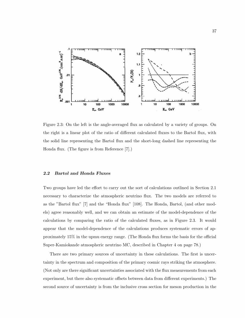
37
Figure 2.3: On the left is the angle-averaged flux as calculated by a variety of groups. On
the right is a linear plot of the ratio of different calculated fluxes to the Bartol flux, with
the solid line representing the Bartol flux and the short-long dashed line representing the
Honda flux. (The figure is from Reference [7].)
2.2 Bartol and Honda Fluxes
Two groups have led the effort to carry out the sort of calculations outlined in Section 2.1
necessary to characterize the atmospheric neutrino flux. The two models are referred to
as the ”Bartol flux” [7] and the “Honda flux” [108]. The Honda, Bartol, (and other mod-
els) agree reasonably well, and we can obtain an estimate of the model-dependence of the
calculations by comparing the ratio of the calculated fluxes, as in Figure 2.3. It would
appear that the model-dependence of the calculations produces systematic errors of ap-
proximately 15% in the upmu energy range. (The Honda flux forms the basis for the official
Super-Kamiokande atmospheric neutrino MC, described in Chapter 4 on page 78.)
There are two primary sources of uncertainty in these calculations. The first is uncer-
tainty in the spectrum and composition of the primary cosmic rays striking the atmosphere.
(Not only are there significant uncertainties associated with the flux measurements from each
experiment, but there also systematic offsets between data from different experiments.) The
second source of uncertainty is from the inclusive cross section for meson production in the
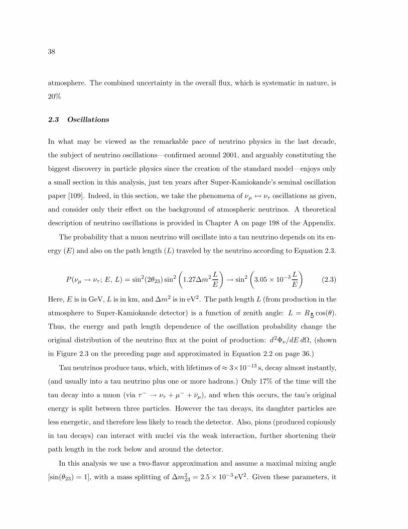
38
atmosphere. The combined uncertainty in the overall flux, which is systematic in nature, is
20%
2.3 Oscillations
In what may be viewed as the remarkable pace of neutrino physics in the last decade,
the subject of neutrino oscillations—confirmed around 2001, and arguably constituting the
biggest discovery in particle physics since the creation of the standard model—enjoys only
a small section in this analysis, just ten years after Super-Kamiokande’s seminal oscillation
paper [109]. Indeed, in this section, we take the phenomena of νµ ↔ ντ oscillations as given,
and consider only their effect on the background of atmospheric neutrinos. A theoretical
description of neutrino oscillations is provided in Chapter A on page 198 of the Appendix.
The probability that a muon neutrino will oscillate into a tau neutrino depends on its en-
ergy (E) and also on the path length (L) traveled by the neutrino according to Equation 2.3.
P (νµ → ντ ; E, L) = sin2(2θ23) sin2
(
1.27∆m2 L
E
)
→ sin2
(
3.05 × 10⁻³ L
E
)
(2.3)
Here, E is in GeV, L is in km, and ∆m2 is in eV2. The path length L (from production in the
atmosphere to Super-Kamiokande detector) is a function of zenith angle: L = R cos(θ).
Thus, the energy and path length dependence of the oscillation probability change the
original distribution of the neutrino flux at the point of production: d2Φν/dE dΩ, (shown
in Figure 2.3 on the preceding page and approximated in Equation 2.2 on page 36.)
Tau neutrinos produce taus, which, with lifetimes of ≈ 3×10⁻¹³ s, decay almost instantly,
(and usually into a tau neutrino plus one or more hadrons.) Only 17% of the time will the
tau decay into a muon (via τ− → ντ + µ− + νµ), and when this occurs, the tau’s original
energy is split between three particles. However the tau decays, its daughter particles are
less energetic, and therefore less likely to reach the detector. Also, pions (produced copiously
in tau decays) can interact with nuclei via the weak interaction, further shortening their
path length in the rock below and around the detector.
In this analysis we use a two-flavor approximation and assume a maximal mixing angle
[sin(θ23) = 1], with a mass splitting of ∆m223 = 2.5 × 10⁻³ eV2. Given these parameters, it
39
0.2 0.4 0.6 0.8 1z=CosHΘL
0.2
0.4
0.6
0.8
1
Psurvival
100 GeV
10 GeV
1 GeV
Figure 2.4: Muon neutrino survival probabilities as a function of cosine of zenith angle at
three different energies.
follows that oscillations are significant for part, but not all, of the upmu energy range. In
Figure 2.4 we plot the survival probabilities as a function of cosine zenith angle for three
different energies. It is apparent that neutrinos in the range of 1−10GeV undergo significant
oscillations, but neutrinos with energies in excess of 100GeV do not (over length scales equal
to R .) Though Super-Kamiokande can not measure energy precisely, it can differentiate
three categories of upmu events, which are correlated with energy, (see Chapter 5.) The
categories from lowest energy to highest energy are: stopping, through-going, and showering.
In Chapter 6 it will be useful to assign each event a weight based on its survival prob-
ability: P (E,L). The weights are a function of zenith angle since zenith angle is related
to path length (L). However, since we do not know the energy (E) of any given event, we
use MC to average over the energy spectrum of each category of event, (denoted m.) We
thereby transform the survival probabilities into functions of zenith angle and event type,
as in Equation 2.4.
P (z,m) =
∫
dE P (z(L), E)P(E|m) (2.4)
Here P(E|m) is the energy spectrum given some category of event.
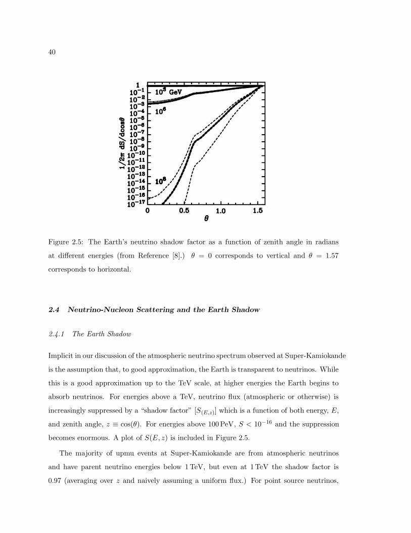
40
Figure 2.5: The Earth’s neutrino shadow factor as a function of zenith angle in radians
at different energies (from Reference [8].) θ = 0 corresponds to vertical and θ = 1.57
corresponds to horizontal.
2.4 Neutrino-Nucleon Scattering and the Earth Shadow
2.4.1 The Earth Shadow
Implicit in our discussion of the atmospheric neutrino spectrum observed at Super-Kamiokande
is the assumption that, to good approximation, the Earth is transparent to neutrinos. While
this is a good approximation up to the TeV scale, at higher energies the Earth begins to
absorb neutrinos. For energies above a TeV, neutrino flux (atmospheric or otherwise) is
increasingly suppressed by a “shadow factor” [S(E,z)] which is a function of both energy, E,
and zenith angle, z ≡ cos(θ). For energies above 100PeV, S < 10−16 and the suppression
becomes enormous. A plot of S(E, z) is included in Figure 2.5.
The majority of upmu events at Super-Kamiokande are from atmospheric neutrinos
and have parent neutrino energies below 1TeV, but even at 1TeV the shadow factor is
0.97 (averaging over z and naively assuming a uniform flux.) For point source neutrinos,
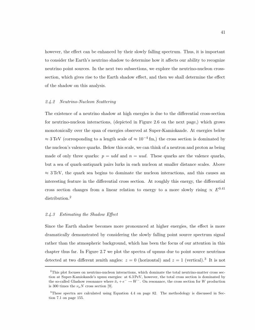
41
however, the effect can be enhanced by their slowly falling spectrum. Thus, it is important
to consider the Earth’s neutrino shadow to determine how it affects our ability to recognize
neutrino point sources. In the next two subsections, we explore the neutrino-nucleon cross-
section, which gives rise to the Earth shadow effect, and then we shall determine the effect
of the shadow on this analysis.
2.4.2 Neutrino-Nucleon Scattering
The existence of a neutrino shadow at high energies is due to the differential cross-section
for neutrino-nucleon interactions, (depicted in Figure 2.6 on the next page,) which grows
monotonically over the span of energies observed at Super-Kamiokande. At energies below
≈ 3TeV (corresponding to a length scale of ≈ 10−4 fm,) the cross section is dominated by
the nucleon’s valence quarks. Below this scale, we can think of a neutron and proton as being
made of only three quarks: p = udd and n = uud. These quarks are the valence quarks,
but a sea of quark-antiquark pairs lurks in each nucleon at smaller distance scales. Above
≈ 3TeV, the quark sea begins to dominate the nucleon interactions, and this causes an
interesting feature in the differential cross section. At roughly this energy, the differential
cross section changes from a linear relation to energy to a more slowly rising ∝ E 0.41
distribution.2
2.4.3 Estimating the Shadow Effect
Since the Earth shadow becomes more pronounced at higher energies, the effect is more
dramatically demonstrated by considering the slowly falling point source spectrum signal
rather than the atmospheric background, which has been the focus of our attention in this
chapter thus far. In Figure 2.7 we plot the spectra of upmus due to point source neutrinos
detected at two different zenith angles: z = 0 (horizontal) and z = 1 (vertical).3 It is not
2This plot focuses on neutrino-nucleon interactions, which dominate the total neutrino-matter cross sec-tion at Super-Kamiokande’s upmu energies: at 6.3 PeV, however, the total cross section is dominated bythe so-called Glashow resonance where νe + e− → W−. On resonance, the cross section for W productionis 300 times the νµN cross section [9].
3These spectra are calculated using Equation 4.4 on page 82. The methodology is discussed in Sec-tion 7.1 on page 155.
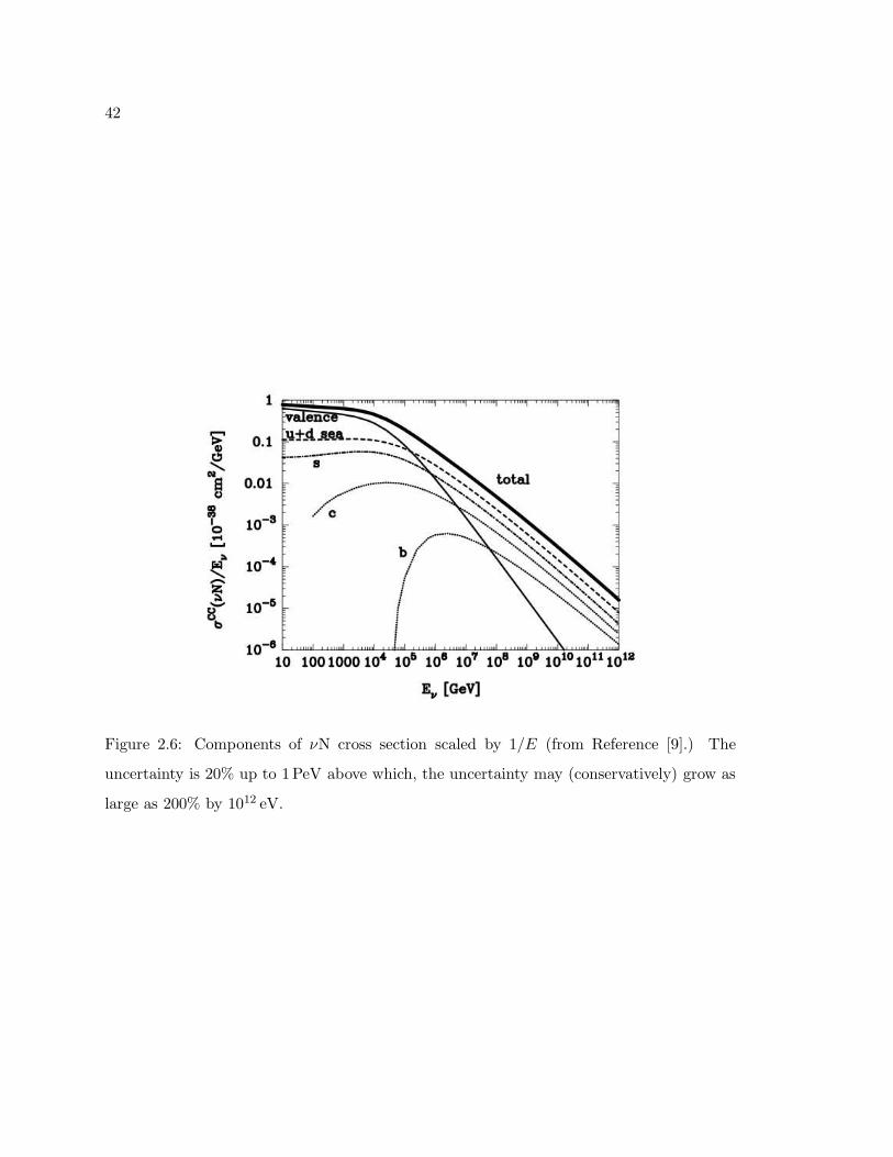
42
Figure 2.6: Components of νN cross section scaled by 1/E (from Reference [9].) The
uncertainty is 20% up to 1PeV above which, the uncertainty may (conservatively) grow as
large as 200% by 1012 eV.
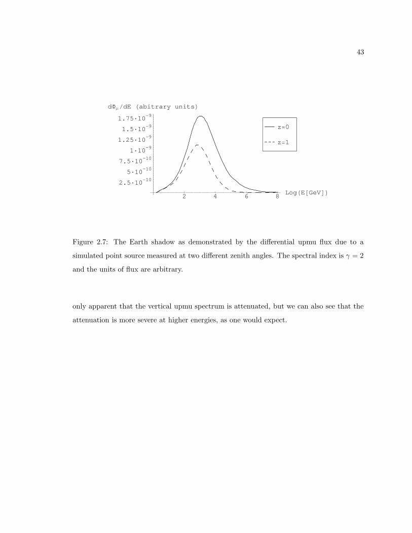
43
2 4 6 [email protected]·10-10
5·10-107.5·10-10
1·10-91.25·10-91.5·10-91.75·10-9
dFΜdE Habitrary unitsLz=1
z=0
Figure 2.7: The Earth shadow as demonstrated by the differential upmu flux due to a
simulated point source measured at two different zenith angles. The spectral index is γ = 2
and the units of flux are arbitrary.
only apparent that the vertical upmu spectrum is attenuated, but we can also see that the
attenuation is more severe at higher energies, as one would expect.
44
Chapter 3
THE SUPER-KAMIOKANDE DETECTOR
3.1 Cherenkov Radiation
Super-Kamiokande relies on the phenomenon of Cherenkov radiation in order to observe
light from charged particles passing through water in the detector. The conical distribution
of Cherenkov radiation allows us to reconstruct the direction of the particle, providing
key information for this analysis. In this section we review and derive the properties of
Cherenkov radiation. Our ultimate goal is: to derive expressions for the Cherenkov angle
(θC) and for the energy loss per unit track length (d2E/dω dx); and also to show that
Cherenkov radiation occurs only for particles that exceed the speed of light in the material
through which they traverse. (Readers in search of information on hardware, electronics,
calibration systems, etc. may wish to omit this section and skip to the next one.)
Given a charged particle moving in the x direction, the easiest way to perform these
calculations is to first calculate the electric and magnetic fields, E and B. (Conveniently,
E3 = B1 = B2 = 0, and so we will really need just three expressions: E1, E2, and B3.) Our
derivation is divided into four steps.
First, we will obtain Fourier expressions for E(k, ω) and B(k, ω). Second, we introduce
a characteristic length, b, which we use to integrate out k. Third, we introduce a character-
istic radiation wavelength, λ−1, which allows us to explore the long range interaction regime
where b >> λ−1. Fourth, we use expressions for E1, E2, and B3 (in the long range interac-
tion regime) to calculate properties of Cherenkov radiation. Following Reference [110], we
work in Gaussian units.
45
3.1.1 Cherenkov Cone Angle
We begin by noting the relationship between four-current and the electromagnetic potential.
∂2Aµ = 4πjµ (3.1)
Here, ∂2 = ∇2 − [ε(ω)/c2] ∂2t , is derived from Maxwell’s equations in linear material. We
consider the case of a charged particle, (in our case, a muon,) traveling in material with a
dielectric constant, ε(ω), and a speed of light vc = c/√
ε(ω). If the particle has velocity, v,
and passes through the position, x at time t = 0, the current is given by:
jµ(x, t) =
q δ(x − v t)
q v δ(x − v t)(3.2)
Here q is one unit of atomic charge. It will be convenient to work in the frequency and wave
number domain, where we can rewrite Equations 3.1 and 3.2 respectively as:
[
k2 − ω2
c2ε(ω)
]
Aµ(k, ω) = 4π jµ(k, ω) (3.3)
and
jµ(k, ω) =
q2π δ(ω − k · v)v φ(k, ω)
(3.4)
where φ(k, ω) ≡ A0(k, ω). Solving Equation 3.3 for Aµ(k, ω), we obtain:
Aµ(k, ω) =
2q δ(ω − k · v)/[
ε(ω)(
k2 − ω2 ε(ω)/c2)]
ε(ω) v
c φ(k, ω)(3.5)
Recalling (half of) the definition of the electromagnetic four-potential, E(x, t) ≡ −∇φ(x, t)−ε(ω)
c∂A(x, t)
∂t , [or E(k, ω) ≡ −ikφ(k, ω)+ ic ω ε(ω)A(k, ω) in the frequency and wave number
domain,] we find the following expression for the electric field:
E(k, ω) = i
(
ω ε(ω)v
c2− k
)
φ(k, ω) (3.6)
Noting that B(x, t) ≡ ∇×A(x, t) [or equivalently B(k, ω) ≡ k×A(k, ω)] we obtain:
B(k, ω) = iε(ω)k × v
cφ(k, ω) (3.7)
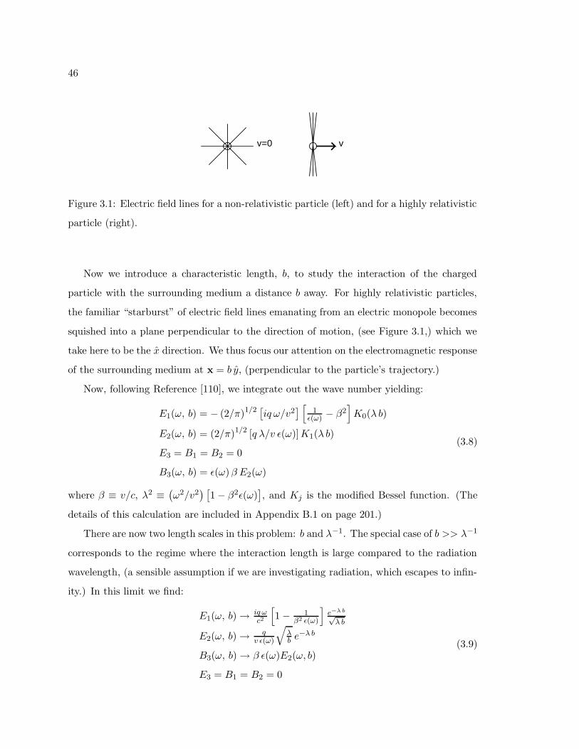
46
vv=0
Figure 3.1: Electric field lines for a non-relativistic particle (left) and for a highly relativistic
particle (right).
Now we introduce a characteristic length, b, to study the interaction of the charged
particle with the surrounding medium a distance b away. For highly relativistic particles,
the familiar “starburst” of electric field lines emanating from an electric monopole becomes
squished into a plane perpendicular to the direction of motion, (see Figure 3.1,) which we
take here to be the x direction. We thus focus our attention on the electromagnetic response
of the surrounding medium at x = b y, (perpendicular to the particle’s trajectory.)
Now, following Reference [110], we integrate out the wave number yielding:
E1(ω, b) = − (2/π)1/2 [iq ω/v2]
[
1ε(ω) − β2
]
K0(λ b)
E2(ω, b) = (2/π)1/2 [q λ/v ε(ω)]K1(λ b)
E3 = B1 = B2 = 0
B3(ω, b) = ε(ω)β E2(ω)
(3.8)
where β ≡ v/c, λ2 ≡(
ω2/v2) [
1 − β2ε(ω)]
, and Kj is the modified Bessel function. (The
details of this calculation are included in Appendix B.1 on page 201.)
There are now two length scales in this problem: b and λ−1. The special case of b >> λ−1
corresponds to the regime where the interaction length is large compared to the radiation
wavelength, (a sensible assumption if we are investigating radiation, which escapes to infin-
ity.) In this limit we find:
E1(ω, b) → iq ωc2
[
1 − 1β2 ε(ω)
]
e−λ b√λ b
E2(ω, b) → qv ε(ω)
√
λb e
−λ b
B3(ω, b) → β ε(ω)E2(ω, b)
E3 = B1 = B2 = 0
(3.9)
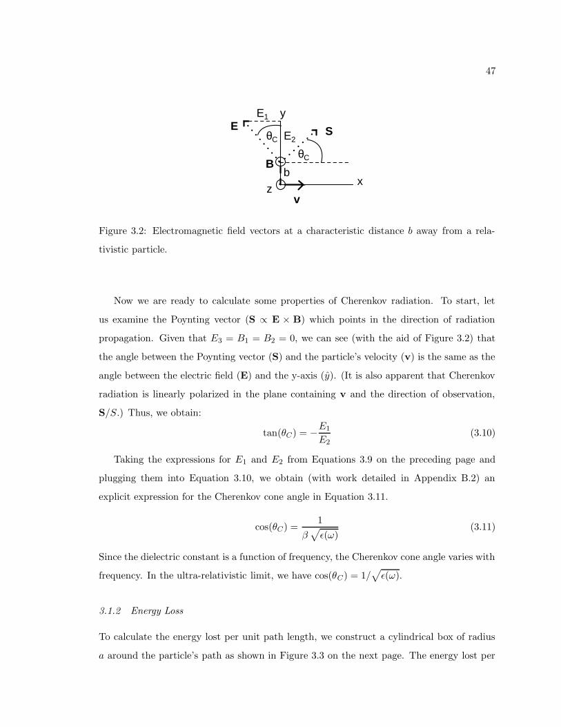
47
x
y
zv
b
θC
θC
E S
.
.
B
E1
E2
Figure 3.2: Electromagnetic field vectors at a characteristic distance b away from a rela-
tivistic particle.
Now we are ready to calculate some properties of Cherenkov radiation. To start, let
us examine the Poynting vector (S ∝ E × B) which points in the direction of radiation
propagation. Given that E3 = B1 = B2 = 0, we can see (with the aid of Figure 3.2) that
the angle between the Poynting vector (S) and the particle’s velocity (v) is the same as the
angle between the electric field (E) and the y-axis (y). (It is also apparent that Cherenkov
radiation is linearly polarized in the plane containing v and the direction of observation,
S/S.) Thus, we obtain:
tan(θC) = −E1
E2(3.10)
Taking the expressions for E1 and E2 from Equations 3.9 on the preceding page and
plugging them into Equation 3.10, we obtain (with work detailed in Appendix B.2) an
explicit expression for the Cherenkov cone angle in Equation 3.11.
cos(θC) =1
β√
ε(ω)(3.11)
Since the dielectric constant is a function of frequency, the Cherenkov cone angle varies with
frequency. In the ultra-relativistic limit, we have cos(θC) = 1/√
ε(ω).
3.1.2 Energy Loss
To calculate the energy lost per unit path length, we construct a cylindrical box of radius
a around the particle’s path as shown in Figure 3.3 on the next page. The energy lost per
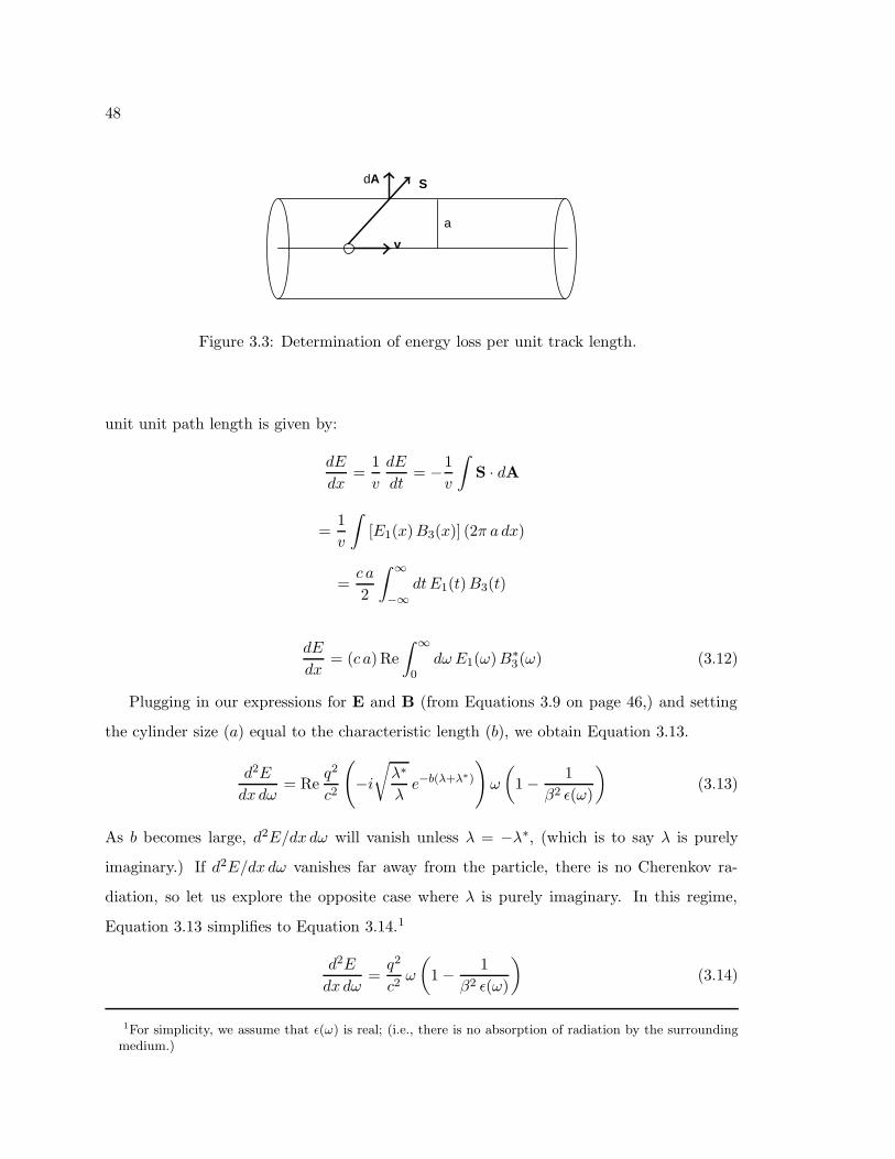
48
v
SAd
a
Figure 3.3: Determination of energy loss per unit track length.
unit unit path length is given by:
dE
dx=
1
v
dE
dt= −1
v
∫
S · dA
=1
v
∫
[E1(x)B3(x)] (2π a dx)
=c a
2
∫ ∞
−∞dtE1(t)B3(t)
dE
dx= (c a)Re
∫ ∞
0dω E1(ω)B∗
3(ω) (3.12)
Plugging in our expressions for E and B (from Equations 3.9 on page 46,) and setting
the cylinder size (a) equal to the characteristic length (b), we obtain Equation 3.13.
d2E
dxdω= Re
q2
c2
(
−i√
λ∗
λe−b(λ+λ∗)
)
ω
(
1 − 1
β2 ε(ω)
)
(3.13)
As b becomes large, d2E/dx dω will vanish unless λ = −λ∗, (which is to say λ is purely
imaginary.) If d2E/dx dω vanishes far away from the particle, there is no Cherenkov ra-
diation, so let us explore the opposite case where λ is purely imaginary. In this regime,
Equation 3.13 simplifies to Equation 3.14.1
d2E
dxdω=q2
c2ω
(
1 − 1
β2 ε(ω)
)
(3.14)
1For simplicity, we assume that ε(ω) is real; (i.e., there is no absorption of radiation by the surroundingmedium.)
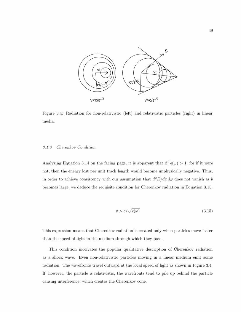
49
vt
ct/ε1/2
v<c/ε1/2 v>c/ε1/2
vt
ct/ε1/2
S
Figure 3.4: Radiation for non-relativistic (left) and relativistic particles (right) in linear
media.
3.1.3 Cherenkov Condition
Analyzing Equation 3.14 on the facing page, it is apparent that β2 ε(ω) > 1, for if it were
not, then the energy lost per unit track length would become unphysically negative. Thus,
in order to achieve consistency with our assumption that d2E/dx dω does not vanish as b
becomes large, we deduce the requisite condition for Cherenkov radiation in Equation 3.15.
v > c/√
ε(ω) (3.15)
This expression means that Cherenkov radiation is created only when particles move faster
than the speed of light in the medium through which they pass.
This condition motivates the popular qualitative description of Cherenkov radiation
as a shock wave. Even non-relativistic particles moving in a linear medium emit some
radiation. The wavefronts travel outward at the local speed of light as shown in Figure 3.4.
If, however, the particle is relativistic, the wavefronts tend to pile up behind the particle
causing interference, which creates the Cherenkov cone.
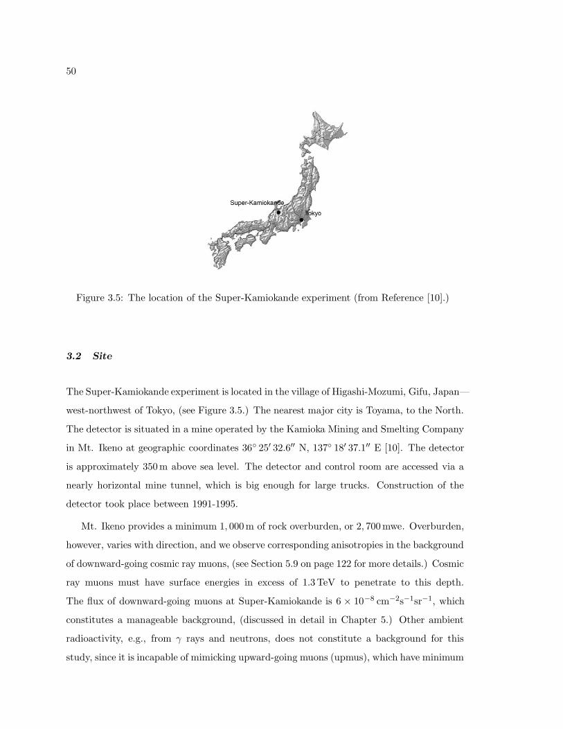
50
Figure 3.5: The location of the Super-Kamiokande experiment (from Reference [10].)
3.2 Site
The Super-Kamiokande experiment is located in the village of Higashi-Mozumi, Gifu, Japan—
west-northwest of Tokyo, (see Figure 3.5.) The nearest major city is Toyama, to the North.
The detector is situated in a mine operated by the Kamioka Mining and Smelting Company
in Mt. Ikeno at geographic coordinates 36 25′ 32.6′′ N, 137 18′ 37.1′′ E [10]. The detector
is approximately 350m above sea level. The detector and control room are accessed via a
nearly horizontal mine tunnel, which is big enough for large trucks. Construction of the
detector took place between 1991-1995.
Mt. Ikeno provides a minimum 1, 000m of rock overburden, or 2, 700mwe. Overburden,
however, varies with direction, and we observe corresponding anisotropies in the background
of downward-going cosmic ray muons, (see Section 5.9 on page 122 for more details.) Cosmic
ray muons must have surface energies in excess of 1.3TeV to penetrate to this depth.
The flux of downward-going muons at Super-Kamiokande is 6 × 10⁻⁸ cm−2s−1sr−1, which
constitutes a manageable background, (discussed in detail in Chapter 5.) Other ambient
radioactivity, e.g., from γ rays and neutrons, does not constitute a background for this
study, since it is incapable of mimicking upward-going muons (upmus), which have minimum
51
energies of 1.6GeV due to cuts described in Chapter 5.
3.3 Detector
In large part, the detector consists of a 50 kton cylindrical tank of ultrapurified water, 39m
in diameter and 42m tall, (see Figure 3.6 on the next page.) It is constructed from welded
stainless steel since the ultrapurified water it contains is highly corrosive. Within the tank
is a stainless steel scaffolding structure, (cylindrical in shape and approximately 2m from
the tank walls,) which divides the tank into an inner detector (ID) and an outer detector
(OD), the latter of which is used as a veto and to shield the ID from radiation in the
surrounding rock. The scaffolding has an inner diameter of 33.8m and a height of 36.2m,
which places 32 ktons of water in the ID. The effective area, determined by requiring that
upmus traverse at least 7m of the ID, varies with zenith angle between ≈ 950 − 1300m2 as
shown in Figure 7.4 on page 159. (The effective area calculation is discussed in greater detail
in Section 7.2.) Though water can pass freely between the ID and OD, the two detectors
are optically separated by specially made sheets consisting of two layers of low-density
polyethylene (LDPE) and one layer of reflective Type 1073B Tyvek R© (manufactured by
the DuPont company.) The sheets are fastened together with plastic pins and stainless steel
staples.
The first 25µm thick layer of LDPE is black and faces the ID. It is designed to absorb as
much light as possible so that light does not bounce around the ID, setting off PMTs outside
the Cherenkov cone of a charged particle and thereby making reconstruction difficult. It
is also desirable to prevent ID light from leaking into the OD and vice versa. Additional
sheets of opaque black polyethylene telephthalate cover the gaps in between ID PMTs to
enhance optical separation of the ID/OD and to improve the absorption of ID light. The
next layer in the optical separation sheet is a 25µm sheet of white LDPE, which along
with the subsequent layer of Tyvek R©, serves to reflect light back into the OD. (The OD
functions more as a veto and calorimeter than as a tracking device, and so—unlike the
ID—it is desirable to minimize absorption in the OD.) A sheet of Tyvek R©, facing the OD,
is the outermost layer of the optical separation sheet.
Tyvek R© is a paper-like substance with several useful traits that make it ideal for the
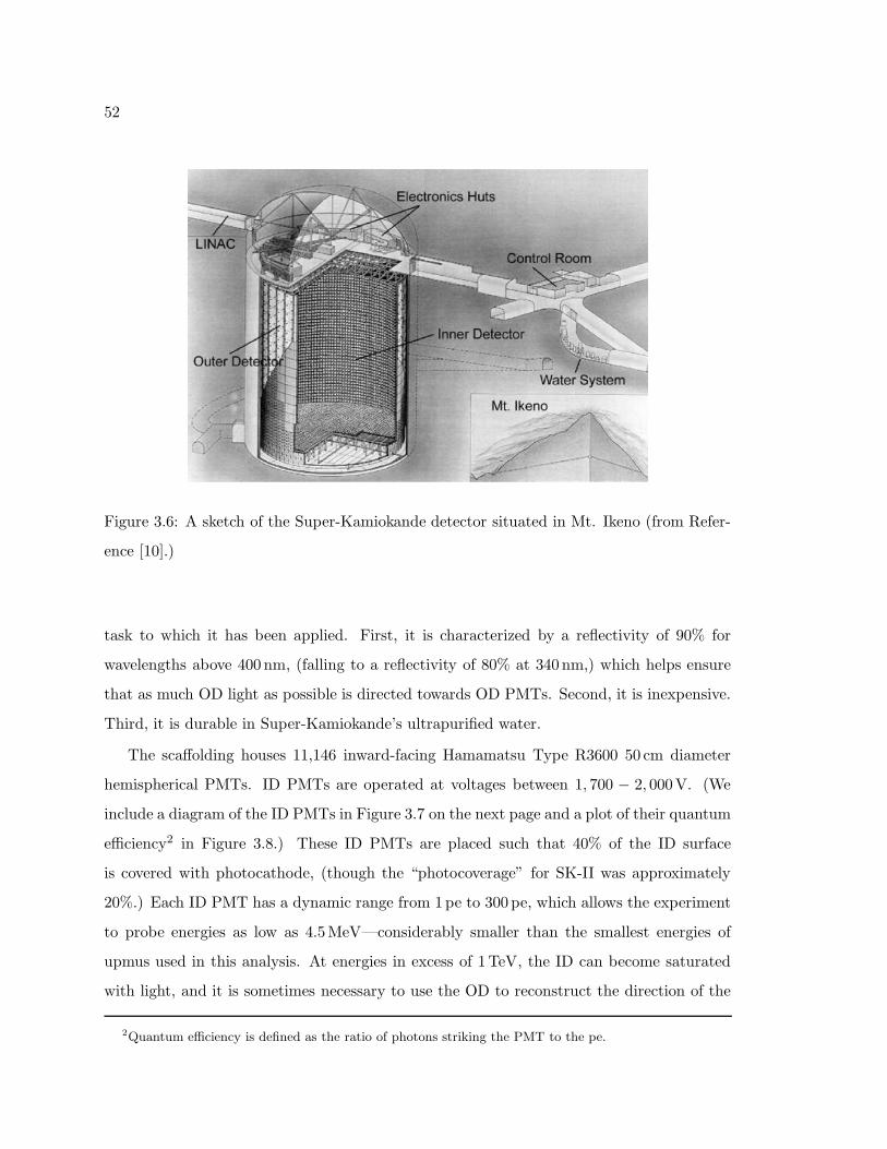
52
Figure 3.6: A sketch of the Super-Kamiokande detector situated in Mt. Ikeno (from Refer-
ence [10].)
task to which it has been applied. First, it is characterized by a reflectivity of 90% for
wavelengths above 400 nm, (falling to a reflectivity of 80% at 340 nm,) which helps ensure
that as much OD light as possible is directed towards OD PMTs. Second, it is inexpensive.
Third, it is durable in Super-Kamiokande’s ultrapurified water.
The scaffolding houses 11,146 inward-facing Hamamatsu Type R3600 50 cm diameter
hemispherical PMTs. ID PMTs are operated at voltages between 1, 700 − 2, 000V. (We
include a diagram of the ID PMTs in Figure 3.7 on the next page and a plot of their quantum
efficiency2 in Figure 3.8.) These ID PMTs are placed such that 40% of the ID surface
is covered with photocathode, (though the “photocoverage” for SK-II was approximately
20%.) Each ID PMT has a dynamic range from 1pe to 300 pe, which allows the experiment
to probe energies as low as 4.5MeV—considerably smaller than the smallest energies of
upmus used in this analysis. At energies in excess of 1TeV, the ID can become saturated
with light, and it is sometimes necessary to use the OD to reconstruct the direction of the
2Quantum efficiency is defined as the ratio of photons striking the PMT to the pe.
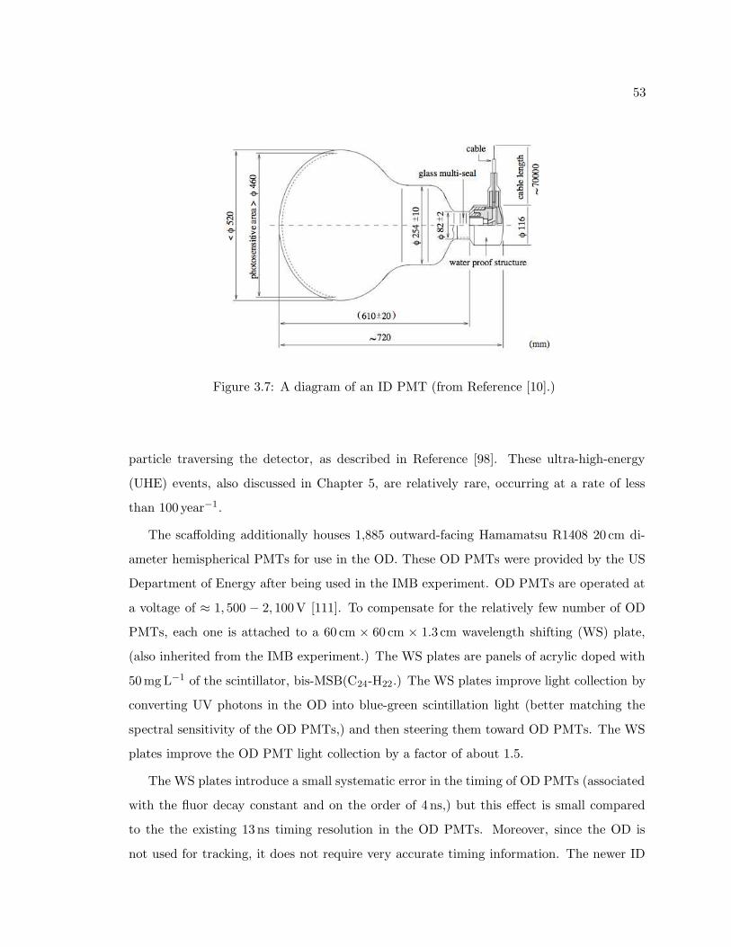
53
Figure 3.7: A diagram of an ID PMT (from Reference [10].)
particle traversing the detector, as described in Reference [98]. These ultra-high-energy
(UHE) events, also discussed in Chapter 5, are relatively rare, occurring at a rate of less
than 100 year−1.
The scaffolding additionally houses 1,885 outward-facing Hamamatsu R1408 20 cm di-
ameter hemispherical PMTs for use in the OD. These OD PMTs were provided by the US
Department of Energy after being used in the IMB experiment. OD PMTs are operated at
a voltage of ≈ 1, 500 − 2, 100V [111]. To compensate for the relatively few number of OD
PMTs, each one is attached to a 60 cm × 60 cm × 1.3 cm wavelength shifting (WS) plate,
(also inherited from the IMB experiment.) The WS plates are panels of acrylic doped with
50mg L−1 of the scintillator, bis-MSB(C24-H22.) The WS plates improve light collection by
converting UV photons in the OD into blue-green scintillation light (better matching the
spectral sensitivity of the OD PMTs,) and then steering them toward OD PMTs. The WS
plates improve the OD PMT light collection by a factor of about 1.5.
The WS plates introduce a small systematic error in the timing of OD PMTs (associated
with the fluor decay constant and on the order of 4 ns,) but this effect is small compared
to the the existing 13 ns timing resolution in the OD PMTs. Moreover, since the OD is
not used for tracking, it does not require very accurate timing information. The newer ID
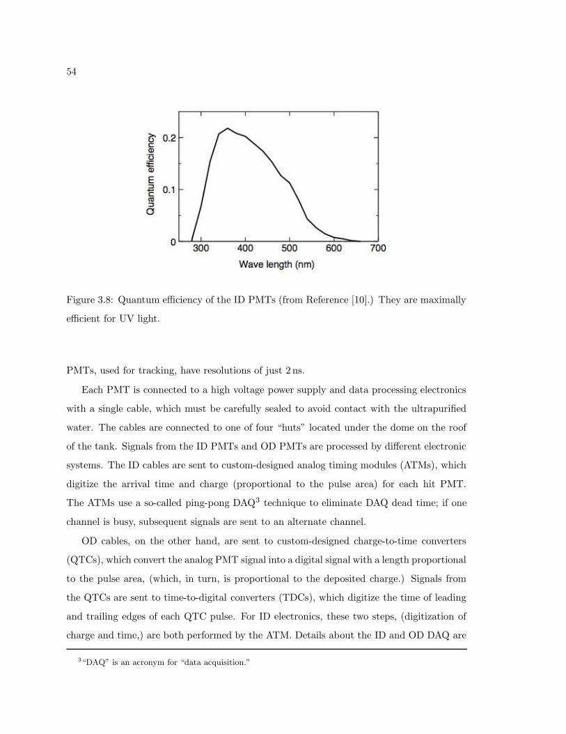
54
Figure 3.8: Quantum efficiency of the ID PMTs (from Reference [10].) They are maximally
efficient for UV light.
PMTs, used for tracking, have resolutions of just 2 ns.
Each PMT is connected to a high voltage power supply and data processing electronics
with a single cable, which must be carefully sealed to avoid contact with the ultrapurified
water. The cables are connected to one of four “huts” located under the dome on the roof
of the tank. Signals from the ID PMTs and OD PMTs are processed by different electronic
systems. The ID cables are sent to custom-designed analog timing modules (ATMs), which
digitize the arrival time and charge (proportional to the pulse area) for each hit PMT.
The ATMs use a so-called ping-pong DAQ3 technique to eliminate DAQ dead time; if one
channel is busy, subsequent signals are sent to an alternate channel.
OD cables, on the other hand, are sent to custom-designed charge-to-time converters
(QTCs), which convert the analog PMT signal into a digital signal with a length proportional
to the pulse area, (which, in turn, is proportional to the deposited charge.) Signals from
the QTCs are sent to time-to-digital converters (TDCs), which digitize the time of leading
and trailing edges of each QTC pulse. For ID electronics, these two steps, (digitization of
charge and time,) are both performed by the ATM. Details about the ID and OD DAQ are
3“DAQ” is an acronym for “data acquisition.”
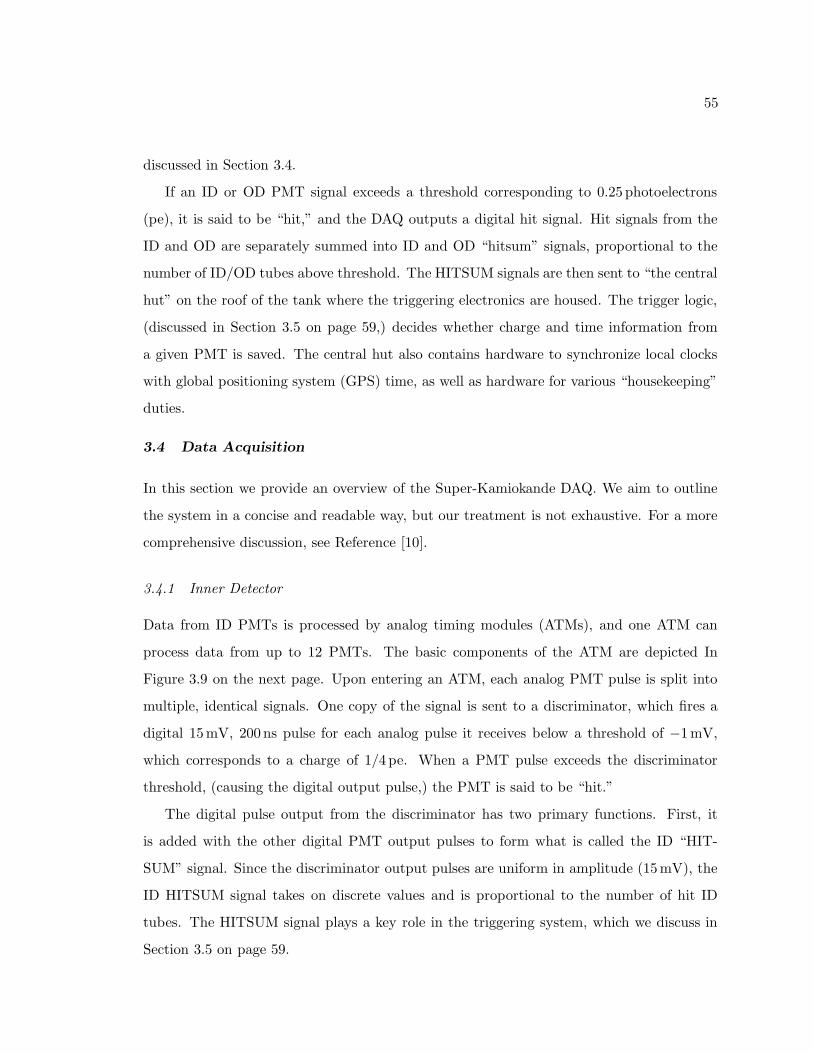
55
discussed in Section 3.4.
If an ID or OD PMT signal exceeds a threshold corresponding to 0.25 photoelectrons
(pe), it is said to be “hit,” and the DAQ outputs a digital hit signal. Hit signals from the
ID and OD are separately summed into ID and OD “hitsum” signals, proportional to the
number of ID/OD tubes above threshold. The HITSUM signals are then sent to “the central
hut” on the roof of the tank where the triggering electronics are housed. The trigger logic,
(discussed in Section 3.5 on page 59,) decides whether charge and time information from
a given PMT is saved. The central hut also contains hardware to synchronize local clocks
with global positioning system (GPS) time, as well as hardware for various “housekeeping”
duties.
3.4 Data Acquisition
In this section we provide an overview of the Super-Kamiokande DAQ. We aim to outline
the system in a concise and readable way, but our treatment is not exhaustive. For a more
comprehensive discussion, see Reference [10].
3.4.1 Inner Detector
Data from ID PMTs is processed by analog timing modules (ATMs), and one ATM can
process data from up to 12 PMTs. The basic components of the ATM are depicted In
Figure 3.9 on the next page. Upon entering an ATM, each analog PMT pulse is split into
multiple, identical signals. One copy of the signal is sent to a discriminator, which fires a
digital 15mV, 200 ns pulse for each analog pulse it receives below a threshold of −1mV,
which corresponds to a charge of 1/4 pe. When a PMT pulse exceeds the discriminator
threshold, (causing the digital output pulse,) the PMT is said to be “hit.”
The digital pulse output from the discriminator has two primary functions. First, it
is added with the other digital PMT output pulses to form what is called the ID “HIT-
SUM” signal. Since the discriminator output pulses are uniform in amplitude (15mV), the
ID HITSUM signal takes on discrete values and is proportional to the number of hit ID
tubes. The HITSUM signal plays a key role in the triggering system, which we discuss in
Section 3.5 on page 59.
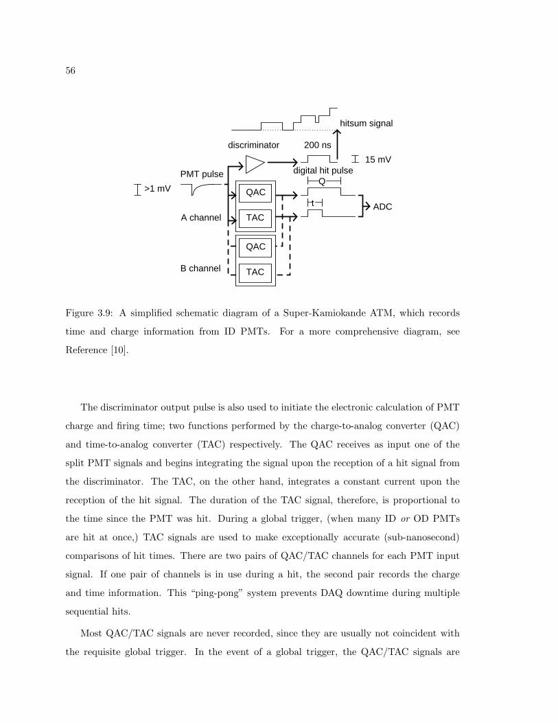
56
PMT pulse
>1 mV
TAC
QAC
discriminator 200 ns
15 mV
Q
t ADC
QAC
TAC
A channel
B channel
digital hit pulse
hitsum signal
Figure 3.9: A simplified schematic diagram of a Super-Kamiokande ATM, which records
time and charge information from ID PMTs. For a more comprehensive diagram, see
Reference [10].
The discriminator output pulse is also used to initiate the electronic calculation of PMT
charge and firing time; two functions performed by the charge-to-analog converter (QAC)
and time-to-analog converter (TAC) respectively. The QAC receives as input one of the
split PMT signals and begins integrating the signal upon the reception of a hit signal from
the discriminator. The TAC, on the other hand, integrates a constant current upon the
reception of the hit signal. The duration of the TAC signal, therefore, is proportional to
the time since the PMT was hit. During a global trigger, (when many ID or OD PMTs
are hit at once,) TAC signals are used to make exceptionally accurate (sub-nanosecond)
comparisons of hit times. There are two pairs of QAC/TAC channels for each PMT input
signal. If one pair of channels is in use during a hit, the second pair records the charge
and time information. This “ping-pong” system prevents DAQ downtime during multiple
sequential hits.
Most QAC/TAC signals are never recorded, since they are usually not coincident with
the requisite global trigger. In the event of a global trigger, the QAC/TAC signals are
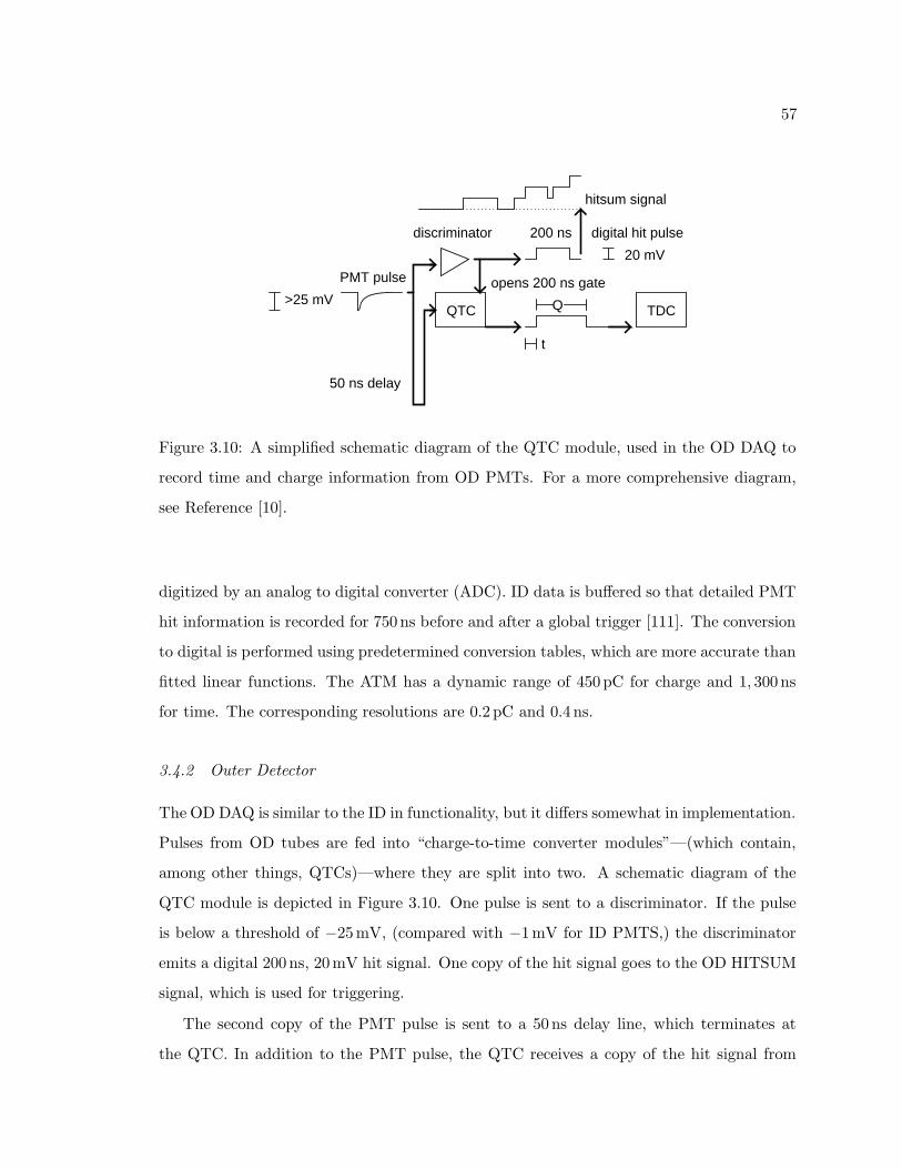
57
PMT pulse
discriminator 200 ns digital hit pulse
hitsum signal
>25 mV
20 mV
50 ns delay
QTC
opens 200 ns gate
Q TDC
t
Figure 3.10: A simplified schematic diagram of the QTC module, used in the OD DAQ to
record time and charge information from OD PMTs. For a more comprehensive diagram,
see Reference [10].
digitized by an analog to digital converter (ADC). ID data is buffered so that detailed PMT
hit information is recorded for 750 ns before and after a global trigger [111]. The conversion
to digital is performed using predetermined conversion tables, which are more accurate than
fitted linear functions. The ATM has a dynamic range of 450 pC for charge and 1, 300 ns
for time. The corresponding resolutions are 0.2 pC and 0.4 ns.
3.4.2 Outer Detector
The OD DAQ is similar to the ID in functionality, but it differs somewhat in implementation.
Pulses from OD tubes are fed into “charge-to-time converter modules”—(which contain,
among other things, QTCs)—where they are split into two. A schematic diagram of the
QTC module is depicted in Figure 3.10. One pulse is sent to a discriminator. If the pulse
is below a threshold of −25mV, (compared with −1mV for ID PMTS,) the discriminator
emits a digital 200 ns, 20mV hit signal. One copy of the hit signal goes to the OD HITSUM
signal, which is used for triggering.
The second copy of the PMT pulse is sent to a 50 ns delay line, which terminates at
the QTC. In addition to the PMT pulse, the QTC receives a copy of the hit signal from
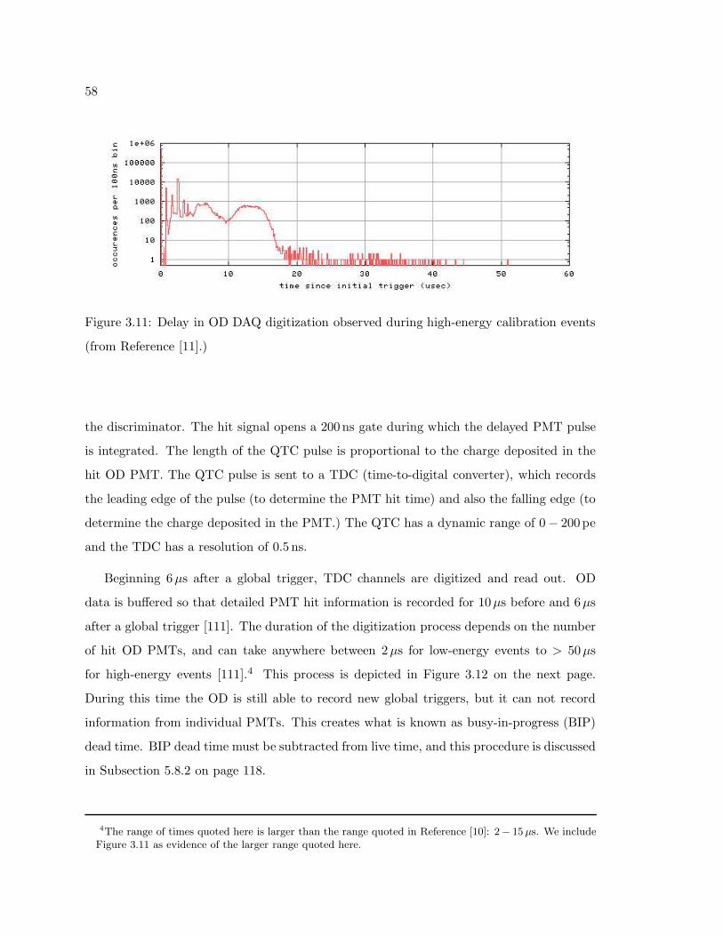
58
Figure 3.11: Delay in OD DAQ digitization observed during high-energy calibration events
(from Reference [11].)
the discriminator. The hit signal opens a 200 ns gate during which the delayed PMT pulse
is integrated. The length of the QTC pulse is proportional to the charge deposited in the
hit OD PMT. The QTC pulse is sent to a TDC (time-to-digital converter), which records
the leading edge of the pulse (to determine the PMT hit time) and also the falling edge (to
determine the charge deposited in the PMT.) The QTC has a dynamic range of 0 − 200 pe
and the TDC has a resolution of 0.5 ns.
Beginning 6µs after a global trigger, TDC channels are digitized and read out. OD
data is buffered so that detailed PMT hit information is recorded for 10µs before and 6µs
after a global trigger [111]. The duration of the digitization process depends on the number
of hit OD PMTs, and can take anywhere between 2µs for low-energy events to > 50µs
for high-energy events [111].4 This process is depicted in Figure 3.12 on the next page.
During this time the OD is still able to record new global triggers, but it can not record
information from individual PMTs. This creates what is known as busy-in-progress (BIP)
dead time. BIP dead time must be subtracted from live time, and this procedure is discussed
in Subsection 5.8.2 on page 118.
4The range of times quoted here is larger than the range quoted in Reference [10]: 2− 15 µs. We includeFigure 3.11 as evidence of the larger range quoted here.
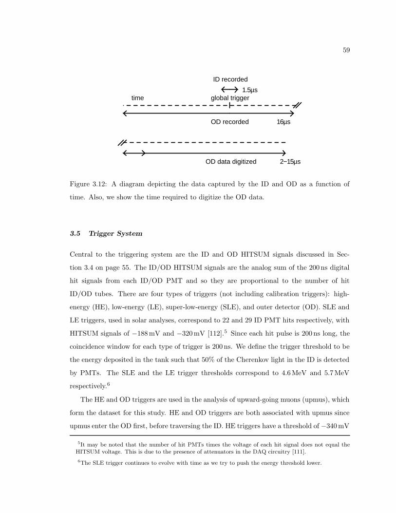
59
time global trigger
ID recorded
OD recorded
1.5µs
16µs
OD data digitized 2−15µs
Figure 3.12: A diagram depicting the data captured by the ID and OD as a function of
time. Also, we show the time required to digitize the OD data.
3.5 Trigger System
Central to the triggering system are the ID and OD HITSUM signals discussed in Sec-
tion 3.4 on page 55. The ID/OD HITSUM signals are the analog sum of the 200 ns digital
hit signals from each ID/OD PMT and so they are proportional to the number of hit
ID/OD tubes. There are four types of triggers (not including calibration triggers): high-
energy (HE), low-energy (LE), super-low-energy (SLE), and outer detector (OD). SLE and
LE triggers, used in solar analyses, correspond to 22 and 29 ID PMT hits respectively, with
HITSUM signals of −188mV and −320mV [112].5 Since each hit pulse is 200 ns long, the
coincidence window for each type of trigger is 200 ns. We define the trigger threshold to be
the energy deposited in the tank such that 50% of the Cherenkov light in the ID is detected
by PMTs. The SLE and the LE trigger thresholds correspond to 4.6MeV and 5.7MeV
respectively.6
The HE and OD triggers are used in the analysis of upward-going muons (upmus), which
form the dataset for this study. HE and OD triggers are both associated with upmus since
upmus enter the OD first, before traversing the ID. HE triggers have a threshold of −340mV
5It may be noted that the number of hit PMTs times the voltage of each hit signal does not equal theHITSUM voltage. This is due to the presence of attenuators in the DAQ circuitry [111].
6The SLE trigger continues to evolve with time as we try to push the energy threshold lower.
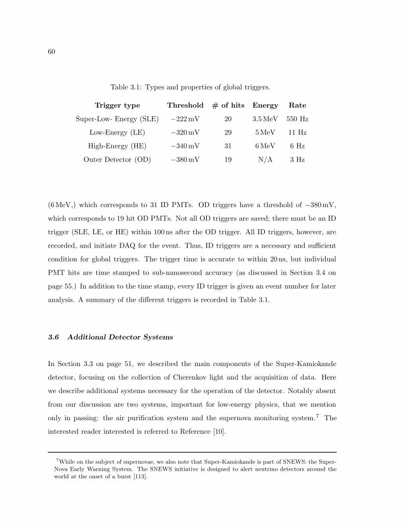
60
Table 3.1: Types and properties of global triggers.
Trigger type Threshold # of hits Energy Rate
Super-Low- Energy (SLE) −222mV 20 3.5MeV 550 Hz
Low-Energy (LE) −320mV 29 5MeV 11 Hz
High-Energy (HE) −340mV 31 6MeV 6 Hz
Outer Detector (OD) −380mV 19 N/A 3 Hz
(6MeV,) which corresponds to 31 ID PMTs. OD triggers have a threshold of −380mV,
which corresponds to 19 hit OD PMTs. Not all OD triggers are saved; there must be an ID
trigger (SLE, LE, or HE) within 100 ns after the OD trigger. All ID triggers, however, are
recorded, and initiate DAQ for the event. Thus, ID triggers are a necessary and sufficient
condition for global triggers. The trigger time is accurate to within 20 ns, but individual
PMT hits are time stamped to sub-nanosecond accuracy (as discussed in Section 3.4 on
page 55.) In addition to the time stamp, every ID trigger is given an event number for later
analysis. A summary of the different triggers is recorded in Table 3.1.
3.6 Additional Detector Systems
In Section 3.3 on page 51, we described the main components of the Super-Kamiokande
detector, focusing on the collection of Cherenkov light and the acquisition of data. Here
we describe additional systems necessary for the operation of the detector. Notably absent
from our discussion are two systems, important for low-energy physics, that we mention
only in passing: the air purification system and the supernova monitoring system.7 The
interested reader interested is referred to Reference [10].
7While on the subject of supernovae, we also note that Super-Kamiokande is part of SNEWS: the Super-Nova Early Warning System. The SNEWS initiative is designed to alert neutrino detectors around theworld at the onset of a burst [113].
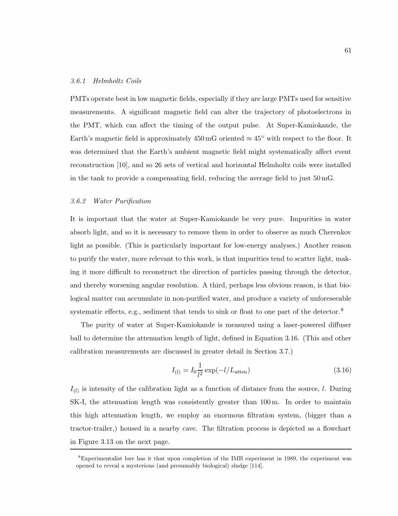
61
3.6.1 Helmholtz Coils
PMTs operate best in low magnetic fields, especially if they are large PMTs used for sensitive
measurements. A significant magnetic field can alter the trajectory of photoelectrons in
the PMT, which can affect the timing of the output pulse. At Super-Kamiokande, the
Earth’s magnetic field is approximately 450mG oriented ≈ 45 with respect to the floor. It
was determined that the Earth’s ambient magnetic field might systematically affect event
reconstruction [10], and so 26 sets of vertical and horizontal Helmholtz coils were installed
in the tank to provide a compensating field, reducing the average field to just 50mG.
3.6.2 Water Purification
It is important that the water at Super-Kamiokande be very pure. Impurities in water
absorb light, and so it is necessary to remove them in order to observe as much Cherenkov
light as possible. (This is particularly important for low-energy analyses.) Another reason
to purify the water, more relevant to this work, is that impurities tend to scatter light, mak-
ing it more difficult to reconstruct the direction of particles passing through the detector,
and thereby worsening angular resolution. A third, perhaps less obvious reason, is that bio-
logical matter can accumulate in non-purified water, and produce a variety of unforeseeable
systematic effects, e.g., sediment that tends to sink or float to one part of the detector.8
The purity of water at Super-Kamiokande is measured using a laser-powered diffuser
ball to determine the attenuation length of light, defined in Equation 3.16. (This and other
calibration measurements are discussed in greater detail in Section 3.7.)
I(l) = I01
l2exp(−l/Latten) (3.16)
I(l) is intensity of the calibration light as a function of distance from the source, l. During
SK-I, the attenuation length was consistently greater than 100m. In order to maintain
this high attenuation length, we employ an enormous filtration system, (bigger than a
tractor-trailer,) housed in a nearby cave. The filtration process is depicted as a flowchart
in Figure 3.13 on the next page.
8Experimentalist lore has it that upon completion of the IMB experiment in 1989, the experiment wasopened to reveal a mysterious (and presumably biological) sludge [114].
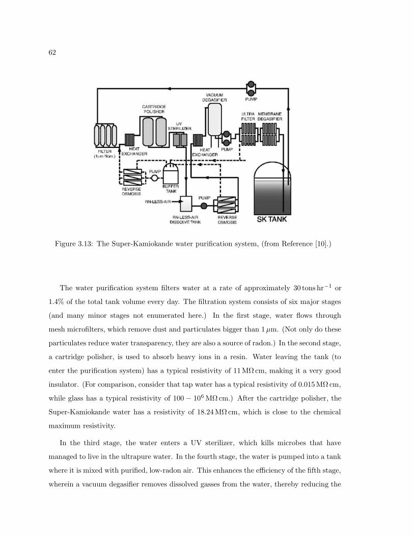
62
Figure 3.13: The Super-Kamiokande water purification system, (from Reference [10].)
The water purification system filters water at a rate of approximately 30 tons hr−1 or
1.4% of the total tank volume every day. The filtration system consists of six major stages
(and many minor stages not enumerated here.) In the first stage, water flows through
mesh microfilters, which remove dust and particulates bigger than 1µm. (Not only do these
particulates reduce water transparency, they are also a source of radon.) In the second stage,
a cartridge polisher, is used to absorb heavy ions in a resin. Water leaving the tank (to
enter the purification system) has a typical resistivity of 11MΩcm, making it a very good
insulator. (For comparison, consider that tap water has a typical resistivity of 0.015MΩcm,
while glass has a typical resistivity of 100 − 106 MΩcm.) After the cartridge polisher, the
Super-Kamiokande water has a resistivity of 18.24MΩcm, which is close to the chemical
maximum resistivity.
In the third stage, the water enters a UV sterilizer, which kills microbes that have
managed to live in the ultrapure water. In the fourth stage, the water is pumped into a tank
where it is mixed with purified, low-radon air. This enhances the efficiency of the fifth stage,
wherein a vacuum degasifier removes dissolved gasses from the water, thereby reducing the
63
dissolved radon. This stage also removes dissolved oxygen, which fosters the growth of some
microbes. After the vacuum degasifier, the oxygen level is about 0.06mg L−1 = 5ppb. (A
pond with oxygen below 2, 000 ppb is considered stagnant, and is unable to support most
species of fish.) Next the water is sent to the sixth and final stage, the membrane degasifier.
The membrane degasifier removes additional radon by pumping the water through thirty
hollow fiber membrane modules.
3.7 Water Transparency Calibration
Water transparency is measured regularly to ensure peak performance of the detector and
to tune the MC. Three techniques are employed to measure water properties: direct mea-
surement with a laser and diffuser ball, indirect measurement with cosmic ray muons, and
scattering measurements with multichromatic lasers.
3.7.1 Direct Measurement
In order to measure the water transparency directly, a diffuser ball is attached to a titanium-
sapphire laser (pumped by a Nd:YAG laser9) and lowered into the tank. The titanium-
sapphire laser lases at 420 nm, but it can be used to probe wavelengths between 350 nm and
500 nm using a second harmonic generator.10 A CCD camera is placed at the top of the ID
to record the intensity of diffuser ball light as a function of distance to the diffuser ball, and
the laser stability is monitored by a small 2 inch PMT, (see Figure 3.14 on the following
page.)
The laser is pulsed in 2 − 3mJ bursts at different depths. At each position the CCD
intensity is recorded normalized by the monitor PMT. The attenuation length, which mea-
sures the water transparency and which we define in Equation 3.16 on page 61, has been
measured to be ≈ 98m (at 420 nm.)
9“Nd:YAG” stands for neodymium-doped yttrium aluminum garnet (Nd:Y3Al5O12). Nd:YAG lasers areoperated in the infrared.
10A second harmonic generator (SHG) uses a crystal to double the frequency of light.
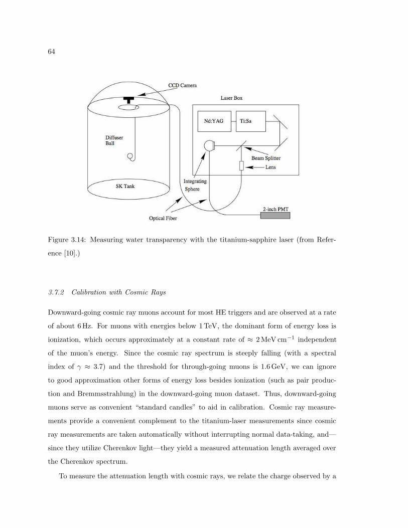
64
Figure 3.14: Measuring water transparency with the titanium-sapphire laser (from Refer-
ence [10].)
3.7.2 Calibration with Cosmic Rays
Downward-going cosmic ray muons account for most HE triggers and are observed at a rate
of about 6Hz. For muons with energies below 1TeV, the dominant form of energy loss is
ionization, which occurs approximately at a constant rate of ≈ 2MeV cm−1 independent
of the muon’s energy. Since the cosmic ray spectrum is steeply falling (with a spectral
index of γ ≈ 3.7) and the threshold for through-going muons is 1.6GeV, we can ignore
to good approximation other forms of energy loss besides ionization (such as pair produc-
tion and Bremmsstrahlung) in the downward-going muon dataset. Thus, downward-going
muons serve as convenient “standard candles” to aid in calibration. Cosmic ray measure-
ments provide a convenient complement to the titanium-laser measurements since cosmic
ray measurements are taken automatically without interrupting normal data-taking, and—
since they utilize Cherenkov light—they yield a measured attenuation length averaged over
the Cherenkov spectrum.
To measure the attenuation length with cosmic rays, we relate the charge observed by a
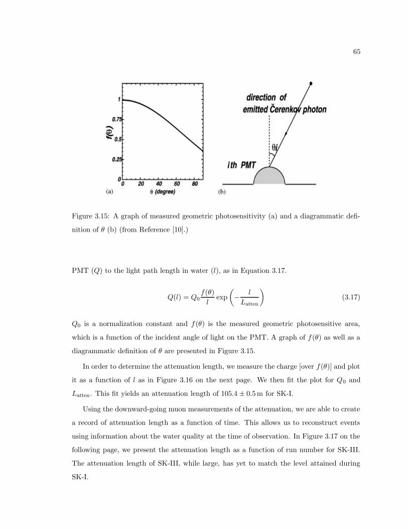
65
Figure 3.15: A graph of measured geometric photosensitivity (a) and a diagrammatic defi-
nition of θ (b) (from Reference [10].)
PMT (Q) to the light path length in water (l), as in Equation 3.17.
Q(l) = Q0f(θ)
lexp
(
− l
Latten
)
(3.17)
Q0 is a normalization constant and f(θ) is the measured geometric photosensitive area,
which is a function of the incident angle of light on the PMT. A graph of f(θ) as well as a
diagrammatic definition of θ are presented in Figure 3.15.
In order to determine the attenuation length, we measure the charge [over f(θ)] and plot
it as a function of l as in Figure 3.16 on the next page. We then fit the plot for Q0 and
Latten. This fit yields an attenuation length of 105.4 ± 0.5m for SK-I.
Using the downward-going muon measurements of the attenuation, we are able to create
a record of attenuation length as a function of time. This allows us to reconstruct events
using information about the water quality at the time of observation. In Figure 3.17 on the
following page, we present the attenuation length as a function of run number for SK-III.
The attenuation length of SK-III, while large, has yet to match the level attained during
SK-I.
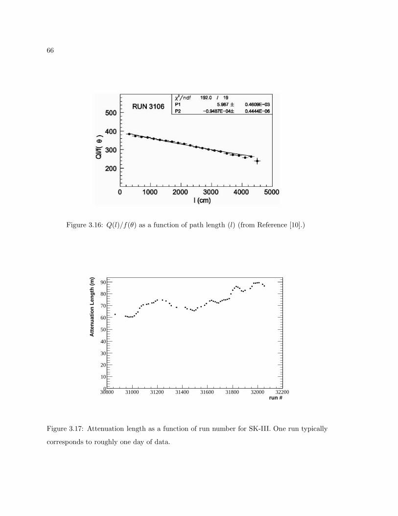
66
Figure 3.16: Q(l)/f(θ) as a function of path length (l) (from Reference [10].)
run #30800 31000 31200 31400 31600 31800 32000 32200
Att
enu
atio
n L
eng
th (
m)
0
10
20
30
40
50
60
70
80
90
Figure 3.17: Attenuation length as a function of run number for SK-III. One run typically
corresponds to roughly one day of data.
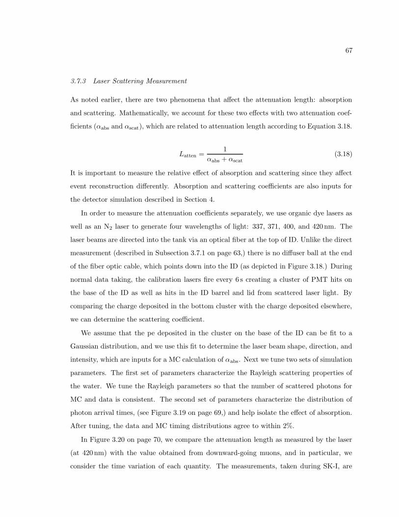
67
3.7.3 Laser Scattering Measurement
As noted earlier, there are two phenomena that affect the attenuation length: absorption
and scattering. Mathematically, we account for these two effects with two attenuation coef-
ficients (αabs and αscat), which are related to attenuation length according to Equation 3.18.
Latten =1
αabs + αscat(3.18)
It is important to measure the relative effect of absorption and scattering since they affect
event reconstruction differently. Absorption and scattering coefficients are also inputs for
the detector simulation described in Section 4.
In order to measure the attenuation coefficients separately, we use organic dye lasers as
well as an N2 laser to generate four wavelengths of light: 337, 371, 400, and 420 nm. The
laser beams are directed into the tank via an optical fiber at the top of ID. Unlike the direct
measurement (described in Subsection 3.7.1 on page 63,) there is no diffuser ball at the end
of the fiber optic cable, which points down into the ID (as depicted in Figure 3.18.) During
normal data taking, the calibration lasers fire every 6 s creating a cluster of PMT hits on
the base of the ID as well as hits in the ID barrel and lid from scattered laser light. By
comparing the charge deposited in the bottom cluster with the charge deposited elsewhere,
we can determine the scattering coefficient.
We assume that the pe deposited in the cluster on the base of the ID can be fit to a
Gaussian distribution, and we use this fit to determine the laser beam shape, direction, and
intensity, which are inputs for a MC calculation of αabs. Next we tune two sets of simulation
parameters. The first set of parameters characterize the Rayleigh scattering properties of
the water. We tune the Rayleigh parameters so that the number of scattered photons for
MC and data is consistent. The second set of parameters characterize the distribution of
photon arrival times, (see Figure 3.19 on page 69,) and help isolate the effect of absorption.
After tuning, the data and MC timing distributions agree to within 2%.
In Figure 3.20 on page 70, we compare the attenuation length as measured by the laser
(at 420 nm) with the value obtained from downward-going muons, and in particular, we
consider the time variation of each quantity. The measurements, taken during SK-I, are

68
Figure 3.18: Laser measurement of the attenuation coefficients (top-left) and a typical
calibration event (bottom-right.) (The image is from from Reference [10].)
found to be consistent to within a few percent.
3.8 Additional Calibration Procedures
Additional calibration procedures are implemented to monitor drift in PMT gain and to
measure timing differences in PMTs. These procedures are discussed below. A plethora of
additional calibration techniques are employed to calibrate the energy scale for fully con-
tained (low-energy) events. These include: LINAC calibration, calibration with radioactive
16N, calibration with a Ni-Cf source, calibration with decay electrons from cosmic ray muons,
calibration of momentum measurements with low-energy stopping muons, and calibration
from neutral pion decay. Since this work focuses on high-energy stopping and through-
going muons—two categories of events for which we can not estimate the energy—we chose
to mention these low-energy calibration procedures only in passing as they have no direct
bearing on this study. The interested reader is directed to Reference [10], which discusses
these procedures in more detail.
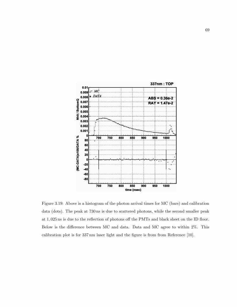
69
Figure 3.19: Above is a histogram of the photon arrival times for MC (bars) and calibration
data (dots). The peak at 730 ns is due to scattered photons, while the second smaller peak
at 1, 025 ns is due to the reflection of photons off the PMTs and black sheet on the ID floor.
Below is the difference between MC and data. Data and MC agree to within 2%. This
calibration plot is for 337 nm laser light and the figure is from from Reference [10].
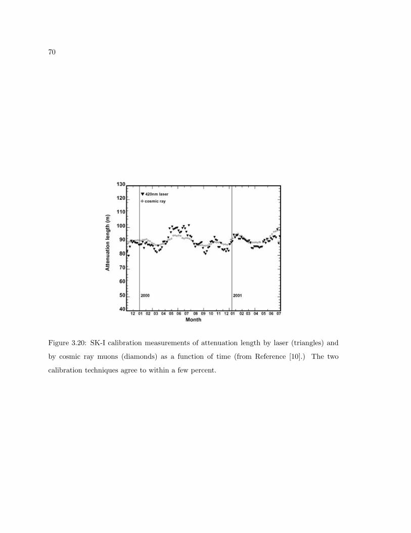
70
Figure 3.20: SK-I calibration measurements of attenuation length by laser (triangles) and
by cosmic ray muons (diamonds) as a function of time (from Reference [10].) The two
calibration techniques agree to within a few percent.
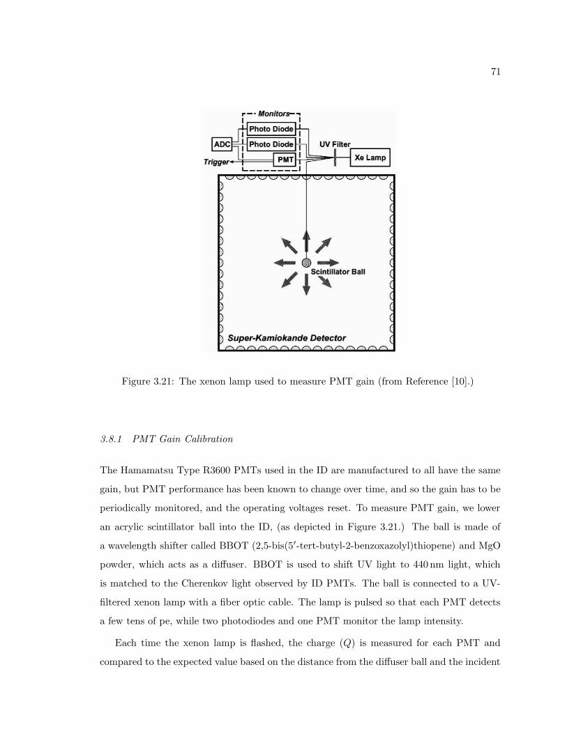
71
Figure 3.21: The xenon lamp used to measure PMT gain (from Reference [10].)
3.8.1 PMT Gain Calibration
The Hamamatsu Type R3600 PMTs used in the ID are manufactured to all have the same
gain, but PMT performance has been known to change over time, and so the gain has to be
periodically monitored, and the operating voltages reset. To measure PMT gain, we lower
an acrylic scintillator ball into the ID, (as depicted in Figure 3.21.) The ball is made of
a wavelength shifter called BBOT (2,5-bis(5′-tert-butyl-2-benzoxazolyl)thiopene) and MgO
powder, which acts as a diffuser. BBOT is used to shift UV light to 440 nm light, which
is matched to the Cherenkov light observed by ID PMTs. The ball is connected to a UV-
filtered xenon lamp with a fiber optic cable. The lamp is pulsed so that each PMT detects
a few tens of pe, while two photodiodes and one PMT monitor the lamp intensity.
Each time the xenon lamp is flashed, the charge (Q) is measured for each PMT and
compared to the expected value based on the distance from the diffuser ball and the incident
72
angle. The relative gain for the ith tube is defined in Equation 3.19.
Gi =Qi
Q0 f(θi)li exp
(
liLatten
)
(3.19)
Here Gi is the gain, Q0 is a constant, f(θi) is geometric photosensitivity (defined in Fig-
ure 3.15,) li is the distance between the PMT and the diffuser ball, and Latten is the atten-
uation length of the water.
Using the calibration data, we define a quantity called “corrected Q,” which corresponds
to the PMT pulse height with corrections to account for differences in the separation between
the diffuser ball and the PMT, the incident angle, and the intensity of the xenon lamp. This
way we can compare the gain of two PMTs in different locations in the ID or at two different
calibration times. Diffuser ball calibration takes place at a variety of heights in order to
minimize any bias resulting from uncertainty in the geometric photosensitivity.
Once we determine the corrected Q for each PMT, we set the operating voltage for each
PMT so that they have the same corrected Q. Some variation persists in the relative PMT
gain distribution, even after tuning; (see Figure 3.22 on the next page.) The persistent
uncertainty in PMT gain distributions is ≈ 7 − 8%. The calibration procedure requires
stoppage of normal data taking and so these measurements are taken only during special
calibration runs.
3.8.2 Relative Timing Calibration
During event reconstruction, we infer information about the arrival time of Cherenkov
photons (and ultimately the trajectory of a charged particle) from the firing times of PMTs,
and so it is critical that we understand and account for any discrepancies in the timing of
different PMTs. Such discrepancies can arise from differences in cable lengths, but a more
challenging problem is that the time between a PMT firing and the output of a digital hit
signal from the ATMs depends on the charge deposited in the PMT. To be more specific,
hit pulses are delayed more as the amount of deposited charge is increased.11 To complicate
matters, the relationship between time and charge is not described by a simple mathematical
11This effect is due to the use of a discriminator in the ID DAQ electronics.
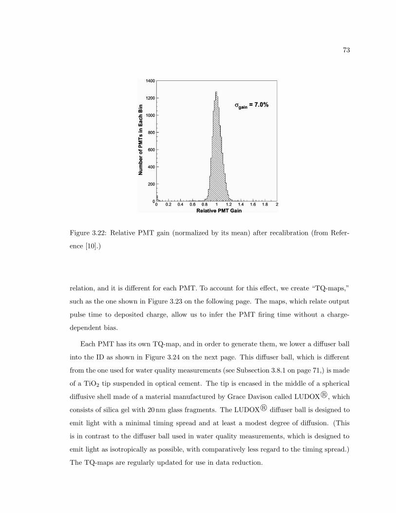
73
Figure 3.22: Relative PMT gain (normalized by its mean) after recalibration (from Refer-
ence [10].)
relation, and it is different for each PMT. To account for this effect, we create “TQ-maps,”
such as the one shown in Figure 3.23 on the following page. The maps, which relate output
pulse time to deposited charge, allow us to infer the PMT firing time without a charge-
dependent bias.
Each PMT has its own TQ-map, and in order to generate them, we lower a diffuser ball
into the ID as shown in Figure 3.24 on the next page. This diffuser ball, which is different
from the one used for water quality measurements (see Subsection 3.8.1 on page 71,) is made
of a TiO2 tip suspended in optical cement. The tip is encased in the middle of a spherical
diffusive shell made of a material manufactured by Grace Davison called LUDOX R©, which
consists of silica gel with 20 nm glass fragments. The LUDOX R© diffuser ball is designed to
emit light with a minimal timing spread and at least a modest degree of diffusion. (This
is in contrast to the diffuser ball used in water quality measurements, which is designed to
emit light as isotropically as possible, with comparatively less regard to the timing spread.)
The TQ-maps are regularly updated for use in data reduction.
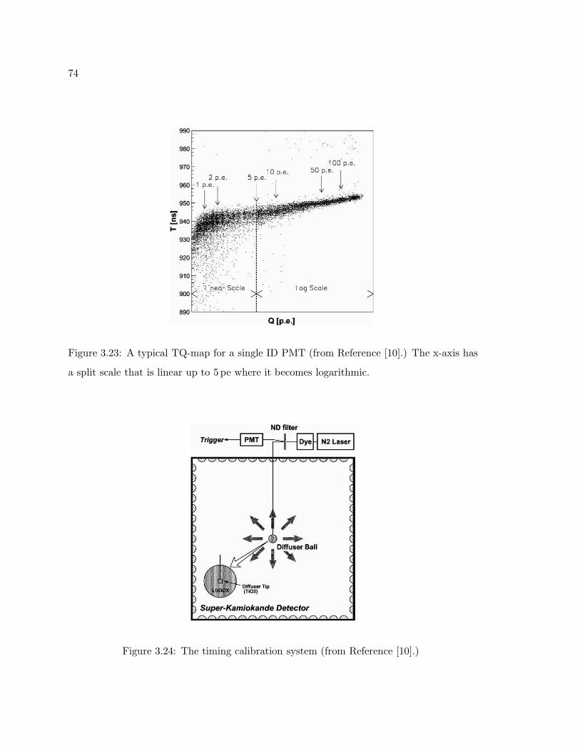
74
Figure 3.23: A typical TQ-map for a single ID PMT (from Reference [10].) The x-axis has
a split scale that is linear up to 5 pe where it becomes logarithmic.
Figure 3.24: The timing calibration system (from Reference [10].)
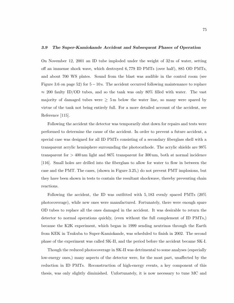
75
3.9 The Super-Kamiokande Accident and Subsequent Phases of Operation
On November 12, 2001 an ID tube imploded under the weight of 32m of water, setting
off an immense shock wave, which destroyed 6, 779 ID PMTs (over half), 885 OD PMTs,
and about 700 WS plates. Sound from the blast was audible in the control room (see
Figure 3.6 on page 52) for 5− 10 s. The accident occurred following maintenance to replace
≈ 200 faulty ID/OD tubes, and so the tank was only 80% filled with water. The vast
majority of damaged tubes were ≥ 5m below the water line, so many were spared by
virtue of the tank not being entirely full. For a more detailed account of the accident, see
Reference [115].
Following the accident the detector was temporarily shut down for repairs and tests were
performed to determine the cause of the accident. In order to prevent a future accident, a
special case was designed for all ID PMTs consisting of a secondary fiberglass shell with a
transparent acrylic hemisphere surrounding the photocathode. The acrylic shields are 98%
transparent for > 400 nm light and 86% transparent for 300 nm, both at normal incidence
[116]. Small holes are drilled into the fiberglass to allow for water to flow in between the
case and the PMT. The cases, (shown in Figure 3.25,) do not prevent PMT implosions, but
they have been shown in tests to contain the resultant shockwave, thereby preventing chain
reactions.
Following the accident, the ID was outfitted with 5, 183 evenly spaced PMTs (20%
photocoverage), while new ones were manufactured. Fortunately, there were enough spare
OD tubes to replace all the ones damaged in the accident. It was desirable to return the
detector to normal operations quickly, (even without the full complement of ID PMTs,)
because the K2K experiment, which began in 1999 sending neutrinos through the Earth
from KEK in Tsukuba to Super-Kamiokande, was scheduled to finish in 2002. The second
phase of the experiment was called SK-II, and the period before the accident became SK-I.
Though the reduced photocoverage in SK-II was detrimental to some analyses (especially
low-energy ones,) many aspects of the detector were, for the most part, unaffected by the
reduction in ID PMTs. Reconstruction of high-energy events, a key component of this
thesis, was only slightly diminished. Unfortunately, it is now necessary to tune MC and
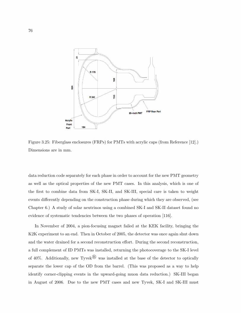
76
Figure 3.25: Fiberglass enclosures (FRPs) for PMTs with acrylic caps (from Reference [12].)
Dimensions are in mm.
data reduction code separately for each phase in order to account for the new PMT geometry
as well as the optical properties of the new PMT cases. In this analysis, which is one of
the first to combine data from SK-I, SK-II, and SK-III, special care is taken to weight
events differently depending on the construction phase during which they are observed, (see
Chapter 6.) A study of solar neutrinos using a combined SK-I and SK-II dataset found no
evidence of systematic tendencies between the two phases of operation [116].
In November of 2004, a pion-focusing magnet failed at the KEK facility, bringing the
K2K experiment to an end. Then in October of 2005, the detector was once again shut down
and the water drained for a second reconstruction effort. During the second reconstruction,
a full complement of ID PMTs was installed, returning the photocoverage to the SK-I level
of 40%. Additionally, new Tyvek R© was installed at the base of the detector to optically
separate the lower cap of the OD from the barrel. (This was proposed as a way to help
identify corner-clipping events in the upward-going muon data reduction.) SK-III began
in August of 2006. Due to the new PMT cases and new Tyvek, SK-I and SK-III must
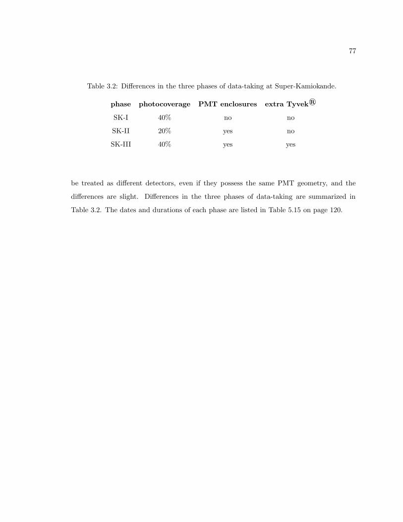
77
Table 3.2: Differences in the three phases of data-taking at Super-Kamiokande.
phase photocoverage PMT enclosures extra Tyvek R©
SK-I 40% no no
SK-II 20% yes no
SK-III 40% yes yes
be treated as different detectors, even if they possess the same PMT geometry, and the
differences are slight. Differences in the three phases of data-taking are summarized in
Table 3.2. The dates and durations of each phase are listed in Table 5.15 on page 120.
78
Chapter 4
MONTE CARLO SIMULATIONS
4.1 Overview
This analysis requires the use of two sets of MC: a set of atmospheric MC to characterize
the background and a set of point source MC to characterize the signal. In both cases, the
generation of MC is divided into four steps, summarized in a flowchart in Figure 4.1 on
the next page. The first step is to characterize the flux of muon neutrinos at the Super-
Kamiokande detector. As discussed in Chapter 2, the flux (d2Φ/dE dΩ) is a function of
energy (E) and zenith angle (z). Tables of d2Φ/dE dΩ used in step one must account for
the various effects (discussed in Chapter 2,) which can distort the flux distribution including
neutrino oscillations and the Earth shadow effect.
The tables of d2Φ/dE dΩ are the input for the second step, which is a simulation
of neutrino-nucleon interactions in and around the detector. In this step, the neutrino
flux tables are used to generate random upmu events based on the input flux and neutrino-
nucleon cross sections encoded into the simulation. Each upmu is assigned a direction and an
energy and propagated to the edge of the detector. The upmu events from step two are the
input to the third step: the detector simulation. The detector simulation is carried out by
a GEANT-based application developed for Super-Kamiokande called skdetsim. skdetsim
propagates the upmus through the detector, generating Cherenkov light, and recording
PMT hits as well as the response of the detector’s DAQ. The end result is a data file, which
is indistinguishable from an actual data file except for the fact that it contains extra banks
of information with MC truth values.
The fourth and final step is to take the data files from step three and plug them
into the upmu reduction described in Chapter 5. The upmu reduction is identical for data
and MC except that we do not perform eye-scanning (see Section 5.7 on page 110) on the
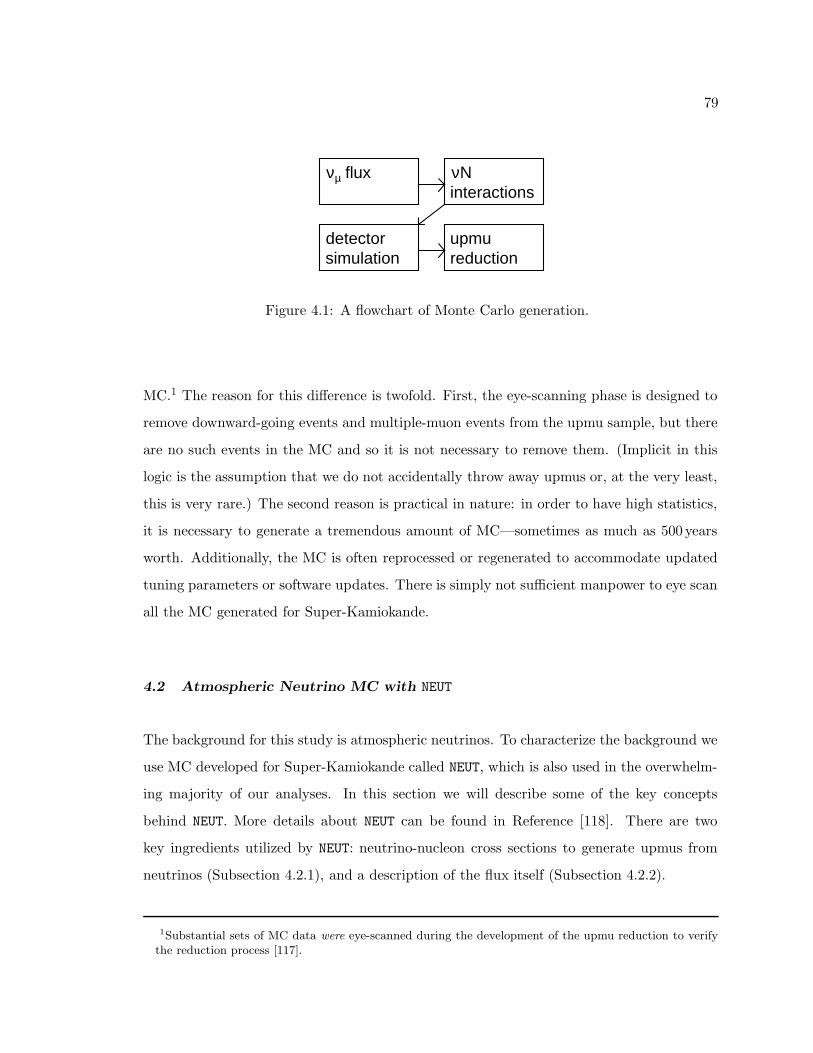
79
νµ flux νN
detectorsimulation
upmureduction
interactions
Figure 4.1: A flowchart of Monte Carlo generation.
MC.1 The reason for this difference is twofold. First, the eye-scanning phase is designed to
remove downward-going events and multiple-muon events from the upmu sample, but there
are no such events in the MC and so it is not necessary to remove them. (Implicit in this
logic is the assumption that we do not accidentally throw away upmus or, at the very least,
this is very rare.) The second reason is practical in nature: in order to have high statistics,
it is necessary to generate a tremendous amount of MC—sometimes as much as 500 years
worth. Additionally, the MC is often reprocessed or regenerated to accommodate updated
tuning parameters or software updates. There is simply not sufficient manpower to eye scan
all the MC generated for Super-Kamiokande.
4.2 Atmospheric Neutrino MC with NEUT
The background for this study is atmospheric neutrinos. To characterize the background we
use MC developed for Super-Kamiokande called NEUT, which is also used in the overwhelm-
ing majority of our analyses. In this section we will describe some of the key concepts
behind NEUT. More details about NEUT can be found in Reference [118]. There are two
key ingredients utilized by NEUT: neutrino-nucleon cross sections to generate upmus from
neutrinos (Subsection 4.2.1), and a description of the flux itself (Subsection 4.2.2).
1Substantial sets of MC data were eye-scanned during the development of the upmu reduction to verifythe reduction process [117].
80
4.2.1 Interactions
NEUT is programmed to simulate a variety of interactions including: quasi-elastic scattering,
single pion production, single kaon production, single η production, coherent pion pro-
duction, and deep inelastic scattering. Only deep inelastic scattering, however, can create
upmus (see Figure 5.1 on page 87,) and so presently we focus on this interaction. In order to
calculate deep inelastic scattering cross sections, NEUT utilizes a parton distribution function
called GRV-94 PDF [119], which models the wave functions of quarks in a nucleus. The
interactions are assumed to take place in “standard rock” with the following properties:
ρ = 2.65 g/cm3, Z = 11, and A = 22 [120]. The propagation of daughter upmus through
rock is simulated by routines developed in Reference [121].
Each upmu has an associated volume through which it may traverse, (given by Equa-
tion 4.1,) which depends on the effective muon range Reff(Ei, Emin), where Ei is the initial
upmu energy and Emin = 1.6GeV is the minimum upmu energy based on cuts described in
Chapter 5.
V µ(Eµ) =4π
3R3
eff (4.1)
The effective detection volume (Veff)—which, consisting of the rock around the detector,
is much bigger than the detector volume—is given by the product of the effective detector
area, Aeff(θ), (a function of zenith angle,) and the muon range, Reff(Ei, Emin).
Veff(E0, θ Emin) = Aeff(θ)Reff(Ei, Emin) (4.2)
We are thus able to constrain the volume around the detector for which events can be
generated by requiring that for each event the ratio of Veff to V µ(Eµ) exceeds a random
number on [0,1] (denoted ζ) [12] as in Equation 4.3.
Veff(E0, θ Emin)/Vµ(Eµ) > ζ (4.3)
We can visualize this requirement by embedding the volume associated with Veff inside
V µ(Eµ). We pick random point inside V µ(Eµ) and accept it if and only if it also lies within
Veff.
81
4.2.2 The Honda Flux
NEUT uses the Honda flux (described in Section 2.2 on page 37) to describe the flux of
atmospheric neutrinos in terms of both angle and energy. The model implemented ranges
from 1GeV to 100TeV. At these energies, the flux is taken to be isotropic in the azimuthal
coordinate φ, but it varies with zenith angle as discussed in Section 2.1 on page 33. The
model does not include contributions from prompt neutrinos (arising from charm decay) as
their effect is negligible at these energies.
4.3 Point Source Monte Carlo
The signal for this study is neutrinos from astrophysical point sources, which we simulate
building on code from Mary Reno (University of Iowa) developed for AMANDA and shared
with Super-Kamiokande via former Super-Kamiokande PhD student, Molly Swanson (MIT)
[122]. This code has been previously used in at least two Super-Kamiokande publications
[14] [98] to calculate the neutrino flux.
The generation of point source MC is divided into two steps. Each event is first assigned
an energy, and then it is assigned an angular deflection (corresponding to the the muon-
neutrino scattering angle as well as scattering during muon propagation.)
4.3.1 Muon Energy
First we use Equations 4.4 and 4.5 to calculate the spectrum of upmu events based on three
ingredients:
• d2Φν
dEν dΩ : the modeled neutrino flux
• P (Eν , Eminµ ): the probability that a neutrino with energy Eν produces a muon with
an energy above Eminµ
• S(z, Eν): the energy and zenith angle dependent Earth shadow (introduced in Chap-
ter 2.4 on page 40)
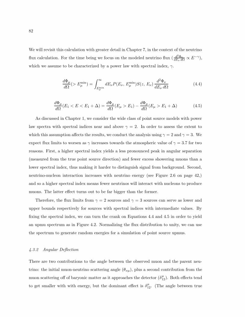
82
We will revisit this calculation with greater detail in Chapter 7, in the context of the neutrino
flux calculation. For the time being we focus on the modeled neutrino flux ( d2Φν
dEν dΩ ∝ E−γ),
which we assume to be characterized by a power law with spectral index, γ.
dΦµ
dΩ(> Emin
µ ) =
∫ ∞
Eminµ
dEνP (Eν , Eminµ )S(z, Eν)
d2Φν
dEν dΩ(4.4)
dΦµ
dΩ(E1 < E < E1 + ∆) =
dΦµ
dΩ(Eµ > E1) −
dΦµ
dΩ(Eµ > E1 + ∆) (4.5)
As discussed in Chapter 1, we consider the wide class of point source models with power
law spectra with spectral indices near and above γ = 2. In order to assess the extent to
which this assumption affects the results, we conduct the analysis using γ = 2 and γ = 3. We
expect flux limits to worsen as γ increases towards the atmospheric value of γ = 3.7 for two
reasons. First, a higher spectral index yields a less pronounced peak in angular separation
(measured from the true point source direction) and fewer excess showering muons than a
lower spectral index, thus making it harder to distinguish signal from background. Second,
neutrino-nucleon interaction increases with neutrino energy (see Figure 2.6 on page 42,)
and so a higher spectral index means fewer neutrinos will interact with nucleons to produce
muons. The latter effect turns out to be far bigger than the former.
Therefore, the flux limits from γ = 2 sources and γ = 3 sources can serve as lower and
upper bounds respectively for sources with spectral indices with intermediate values. By
fixing the spectral index, we can turn the crank on Equations 4.4 and 4.5 in order to yield
an upmu spectrum as in Figure 4.2. Normalizing the flux distribution to unity, we can use
the spectrum to generate random energies for a simulation of point source upmus.
4.3.2 Angular Deflection
There are two contributions to the angle between the observed muon and the parent neu-
trino: the initial muon-neutrino scattering angle (θνµ), plus a second contribution from the
muon scattering off of baryonic matter as it approaches the detector (δµ12). Both effects tend
to get smaller with with energy, but the dominant effect is δµ12. (The angle between true
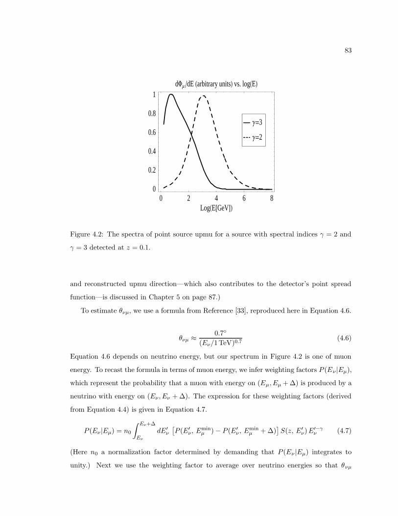
83
0 2 4 6 8LogHE@GeVDL0
0.2
0.4
0.6
0.8
1dFΜ dE Harbitrary unitsL vs. logHEL
Γ=2
Γ=3
Figure 4.2: The spectra of point source upmu for a source with spectral indices γ = 2 and
γ = 3 detected at z = 0.1.
and reconstructed upmu direction—which also contributes to the detector’s point spread
function—is discussed in Chapter 5 on page 87.)
To estimate θνµ, we use a formula from Reference [33], reproduced here in Equation 4.6.
θνµ ≈ 0.7
(Eν/1TeV)0.7(4.6)
Equation 4.6 depends on neutrino energy, but our spectrum in Figure 4.2 is one of muon
energy. To recast the formula in terms of muon energy, we infer weighting factors P (Eν |Eµ),
which represent the probability that a muon with energy on (Eµ, Eµ + ∆) is produced by a
neutrino with energy on (Eν , Eν + ∆). The expression for these weighting factors (derived
from Equation 4.4) is given in Equation 4.7.
P (Eν |Eµ) = n0
∫ Eν+∆
Eν
dE′ν
[
P (E′ν , E
minµ ) − P (E′
ν , Eminµ + ∆)
]
S(z, E′ν)E
′−γν (4.7)
(Here n0 a normalization factor determined by demanding that P (Eν |Eµ) integrates to
unity.) Next we use the weighting factor to average over neutrino energies so that θνµ
84
depends only on upmu energy as in Equation 4.8.
θνµ(Eµ) =∑
Eν
0.7
(Eν/1TeV)0.7P (Eν |Eµ) (4.8)
Since point source parent neutrino spectrum is so steep, the angular deflection due to
neutrino-muon scattering is small: on the order of 0.2 or less. We shall see that the
contribution to angular deflection from δµ12 is much bigger.
To estimate δµ12, (the angular deflection that occurs when the muon scatters off baryonic
matter,) we use the existing atmospheric MC, which models this scattering using GEANT 3.
We create histograms of angular separation between muon direction at the point of creation
(in the rock around the detector) and the muon direction at the entrance to the detector at
different muon energies. Then each MC event is assigned a random value for δµ12 based on its
muon energy. The angle δµ12 is can be as big as several degrees (at low energies), making it
significantly more important than the contribution from neutrino-muon scattering, although
both effects are smaller than the angular resolution of the detector at typical point source
energies. To account for both effects, the total angular deflection is given by the sum in
quadrature of θνµ and δµ12. The total angular deflection, which is a function of muon energy,
is depicted in Figure 4.3.
In Subsection 4.3.1 on page 81 we described how each event was assigned a randomly
generated upmu energy according to the upmu energy spectrum. Now we use the distri-
bution shown in Figure 4.3 to determine the average deflection for each upmu energy. We
generate a random deflection by assuming that deflections are normally distributed about
zero with a standard deviation given by the average angular deflection. (The sign of the
deflection determines whether the upmu is deflected up or down in the z coordinate.)
The last step is to convert the upmu energy and angular deflection into a vector, which
can be used as input for the detector simulation. We carry out this step by assuming the
point source illuminates the detector with a uniform beam. Then we calculate the entrance
points using simple geometry.
4.4 skdetsim
skdetsim is a GEANT 3 based detector simulation, which has likely been used in every
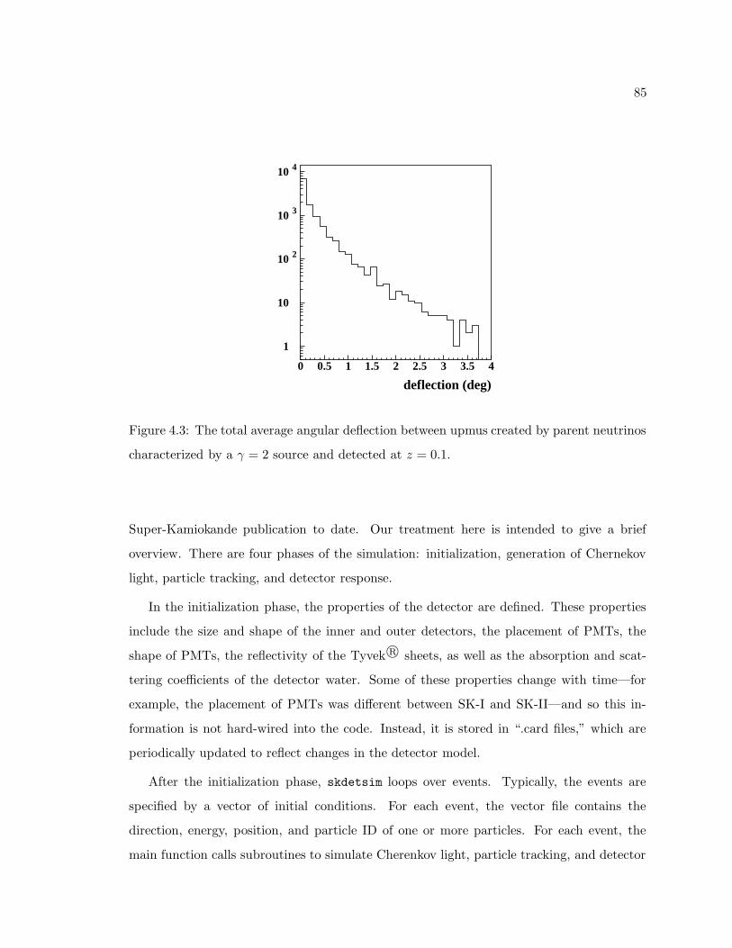
85
deflection (deg)
1
10
10 2
10 3
10 4
0 0.5 1 1.5 2 2.5 3 3.5 4
Figure 4.3: The total average angular deflection between upmus created by parent neutrinos
characterized by a γ = 2 source and detected at z = 0.1.
Super-Kamiokande publication to date. Our treatment here is intended to give a brief
overview. There are four phases of the simulation: initialization, generation of Chernekov
light, particle tracking, and detector response.
In the initialization phase, the properties of the detector are defined. These properties
include the size and shape of the inner and outer detectors, the placement of PMTs, the
shape of PMTs, the reflectivity of the Tyvek R© sheets, as well as the absorption and scat-
tering coefficients of the detector water. Some of these properties change with time—for
example, the placement of PMTs was different between SK-I and SK-II—and so this in-
formation is not hard-wired into the code. Instead, it is stored in “.card files,” which are
periodically updated to reflect changes in the detector model.
After the initialization phase, skdetsim loops over events. Typically, the events are
specified by a vector of initial conditions. For each event, the vector file contains the
direction, energy, position, and particle ID of one or more particles. For each event, the
main function calls subroutines to simulate Cherenkov light, particle tracking, and detector
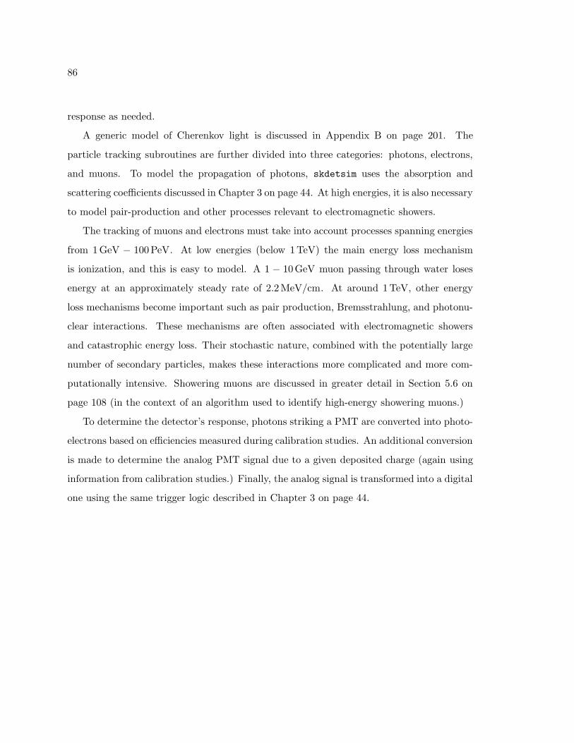
86
response as needed.
A generic model of Cherenkov light is discussed in Appendix B on page 201. The
particle tracking subroutines are further divided into three categories: photons, electrons,
and muons. To model the propagation of photons, skdetsim uses the absorption and
scattering coefficients discussed in Chapter 3 on page 44. At high energies, it is also necessary
to model pair-production and other processes relevant to electromagnetic showers.
The tracking of muons and electrons must take into account processes spanning energies
from 1GeV − 100PeV. At low energies (below 1TeV) the main energy loss mechanism
is ionization, and this is easy to model. A 1 − 10GeV muon passing through water loses
energy at an approximately steady rate of 2.2MeV/cm. At around 1TeV, other energy
loss mechanisms become important such as pair production, Bremsstrahlung, and photonu-
clear interactions. These mechanisms are often associated with electromagnetic showers
and catastrophic energy loss. Their stochastic nature, combined with the potentially large
number of secondary particles, makes these interactions more complicated and more com-
putationally intensive. Showering muons are discussed in greater detail in Section 5.6 on
page 108 (in the context of an algorithm used to identify high-energy showering muons.)
To determine the detector’s response, photons striking a PMT are converted into photo-
electrons based on efficiencies measured during calibration studies. An additional conversion
is made to determine the analog PMT signal due to a given deposited charge (again using
information from calibration studies.) Finally, the analog signal is transformed into a digital
one using the same trigger logic described in Chapter 3 on page 44.
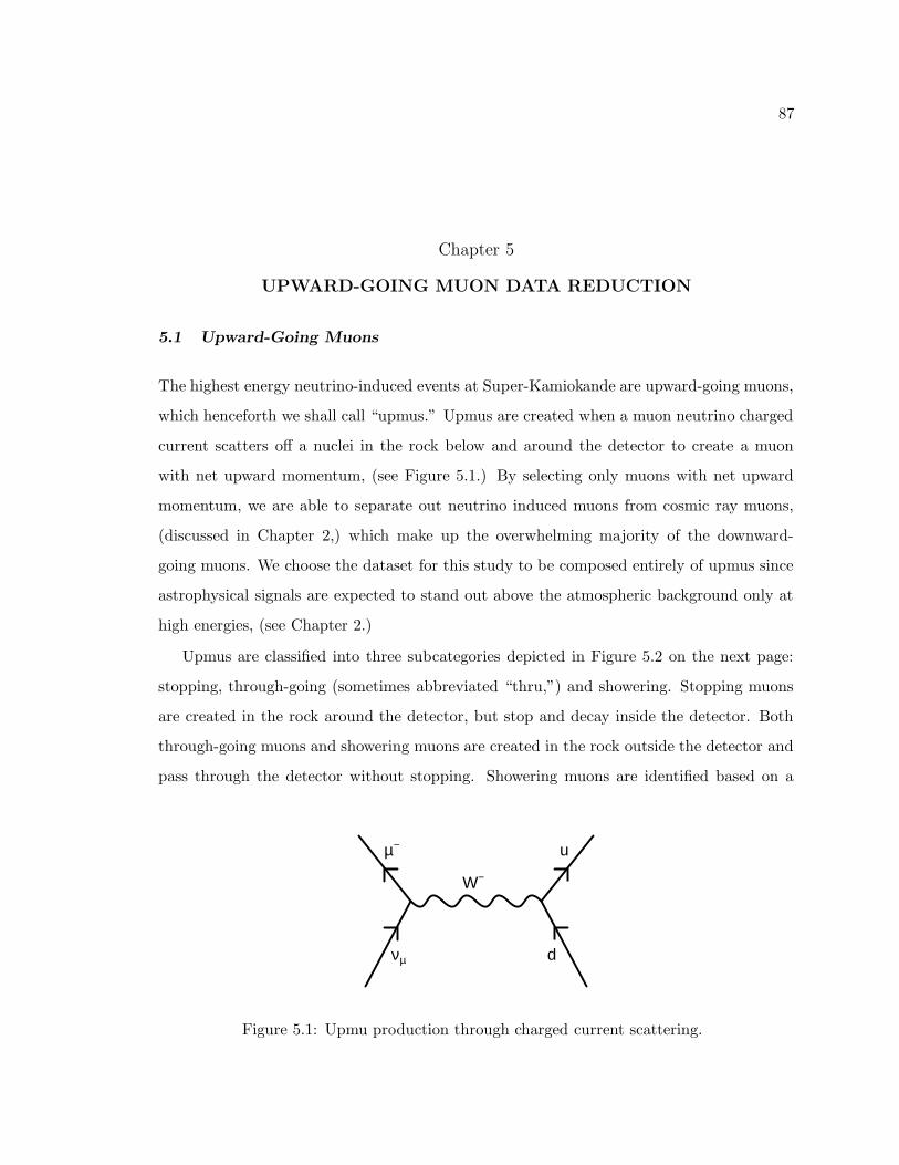
87
Chapter 5
UPWARD-GOING MUON DATA REDUCTION
5.1 Upward-Going Muons
The highest energy neutrino-induced events at Super-Kamiokande are upward-going muons,
which henceforth we shall call “upmus.” Upmus are created when a muon neutrino charged
current scatters off a nuclei in the rock below and around the detector to create a muon
with net upward momentum, (see Figure 5.1.) By selecting only muons with net upward
momentum, we are able to separate out neutrino induced muons from cosmic ray muons,
(discussed in Chapter 2,) which make up the overwhelming majority of the downward-
going muons. We choose the dataset for this study to be composed entirely of upmus since
astrophysical signals are expected to stand out above the atmospheric background only at
high energies, (see Chapter 2.)
Upmus are classified into three subcategories depicted in Figure 5.2 on the next page:
stopping, through-going (sometimes abbreviated “thru,”) and showering. Stopping muons
are created in the rock around the detector, but stop and decay inside the detector. Both
through-going muons and showering muons are created in the rock outside the detector and
pass through the detector without stopping. Showering muons are identified based on a
νµ d
uµ−
W−
Figure 5.1: Upmu production through charged current scattering.
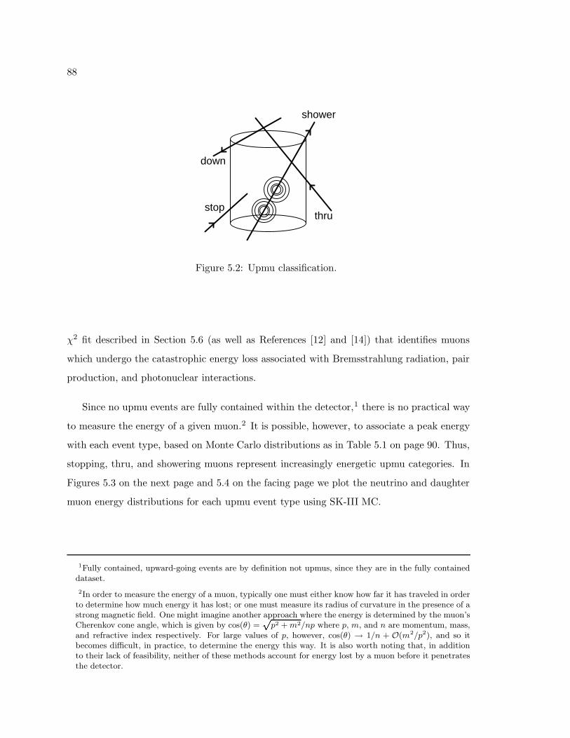
88
thru
shower
stop
down
Figure 5.2: Upmu classification.
χ2 fit described in Section 5.6 (as well as References [12] and [14]) that identifies muons
which undergo the catastrophic energy loss associated with Bremsstrahlung radiation, pair
production, and photonuclear interactions.
Since no upmu events are fully contained within the detector,1 there is no practical way
to measure the energy of a given muon.2 It is possible, however, to associate a peak energy
with each event type, based on Monte Carlo distributions as in Table 5.1 on page 90. Thus,
stopping, thru, and showering muons represent increasingly energetic upmu categories. In
Figures 5.3 on the next page and 5.4 on the facing page we plot the neutrino and daughter
muon energy distributions for each upmu event type using SK-III MC.
1Fully contained, upward-going events are by definition not upmus, since they are in the fully containeddataset.
2In order to measure the energy of a muon, typically one must either know how far it has traveled in orderto determine how much energy it has lost; or one must measure its radius of curvature in the presence of astrong magnetic field. One might imagine another approach where the energy is determined by the muon’sCherenkov cone angle, which is given by cos(θ) = p2 + m2/np where p, m, and n are momentum, mass,and refractive index respectively. For large values of p, however, cos(θ) → 1/n + O(m2/p2), and so itbecomes difficult, in practice, to determine the energy this way. It is also worth noting that, in additionto their lack of feasibility, neither of these methods account for energy lost by a muon before it penetratesthe detector.
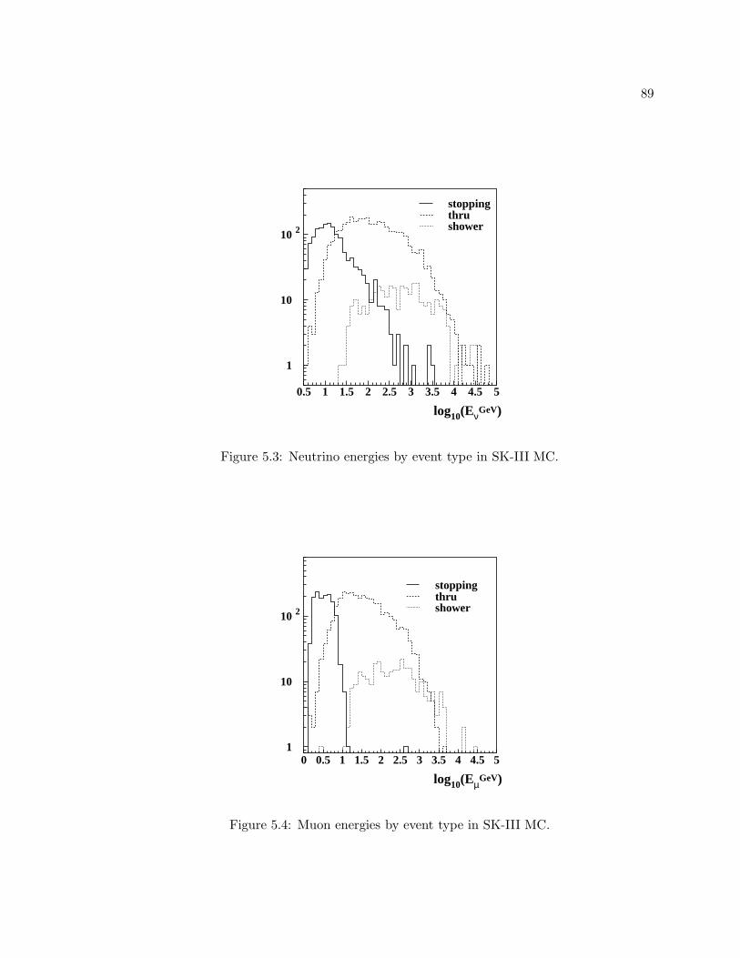
89
log10(EνGeV)
stoppingthrushower
1
10
10 2
0.5 1 1.5 2 2.5 3 3.5 4 4.5 5
Figure 5.3: Neutrino energies by event type in SK-III MC.
log10(EµGeV)
stoppingthrushower
1
10
10 2
0 0.5 1 1.5 2 2.5 3 3.5 4 4.5 5
Figure 5.4: Muon energies by event type in SK-III MC.
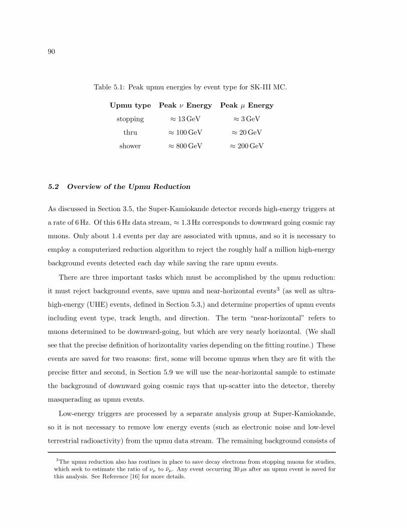
90
Table 5.1: Peak upmu energies by event type for SK-III MC.
Upmu type Peak ν Energy Peak µ Energy
stopping ≈ 13GeV ≈ 3GeV
thru ≈ 100GeV ≈ 20GeV
shower ≈ 800GeV ≈ 200GeV
5.2 Overview of the Upmu Reduction
As discussed in Section 3.5, the Super-Kamiokande detector records high-energy triggers at
a rate of 6Hz. Of this 6Hz data stream, ≈ 1.3Hz corresponds to downward going cosmic ray
muons. Only about 1.4 events per day are associated with upmus, and so it is necessary to
employ a computerized reduction algorithm to reject the roughly half a million high-energy
background events detected each day while saving the rare upmu events.
There are three important tasks which must be accomplished by the upmu reduction:
it must reject background events, save upmu and near-horizontal events3 (as well as ultra-
high-energy (UHE) events, defined in Section 5.3,) and determine properties of upmu events
including event type, track length, and direction. The term “near-horizontal” refers to
muons determined to be downward-going, but which are very nearly horizontal. (We shall
see that the precise definition of horizontality varies depending on the fitting routine.) These
events are saved for two reasons: first, some will become upmus when they are fit with the
precise fitter and second, in Section 5.9 we will use the near-horizontal sample to estimate
the background of downward going cosmic rays that up-scatter into the detector, thereby
masquerading as upmu events.
Low-energy triggers are processed by a separate analysis group at Super-Kamiokande,
so it is not necessary to remove low energy events (such as electronic noise and low-level
terrestrial radioactivity) from the upmu data stream. The remaining background consists of
3The upmu reduction also has routines in place to save decay electrons from stopping muons for studies,which seek to estimate the ratio of νµ to νµ. Any event occurring 30 µs after an upmu event is saved forthis analysis. See Reference [16] for more details.
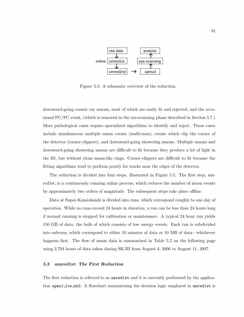
91
umred1st eye-scanning
umred2nd upmu3
analysis
online:
raw data
Figure 5.5: A schematic overview of the reduction.
downward-going cosmic ray muons, most of which are easily fit and rejected, and the occa-
sional PC/FC event, (which is removed in the eye-scanning phase described in Section 5.7.)
More pathological cases require specialized algorithms to identify and reject. These cases
include simultaneous multiple muon events (multi-mus), events which clip the corner of
the detector (corner-clippers), and downward-going showering muons. Multiple muons and
downward-going showering muons are difficult to fit because they produce a lot of light in
the ID, but without clean muon-like rings. Corner-clippers are difficult to fit because the
fitting algorithms tend to perform poorly for tracks near the edges of the detector.
The reduction is divided into four steps, illustrated in Figure 5.5. The first step, um-
red1st, is a continuously running online process, which reduces the number of muon events
by approximately two orders of magnitude. The subsequent steps take place offline.
Data at Super-Kamiokande is divided into runs, which correspond roughly to one day of
operation. While no runs exceed 24 hours in duration, a run can be less than 24 hours long
if normal running is stopped for calibration or maintenance. A typical 24 hour run yields
150 GB of data, the bulk of which consists of low energy events. Each run is subdivided
into subruns, which correspond to either 10 minutes of data or 10 MB of data—whichever
happens first. The flow of muon data is summarized in Table 5.2 on the following page
using 2,704 hours of data taken during SK-III from August 4, 2006 to August 11, 2007.
5.3 umred1st: The First Reduction
The first reduction is referred to as umred1st and it is currently performed by the applica-
tion upmu1 low sk3. A flowchart summarizing the decision logic employed in umred1st is
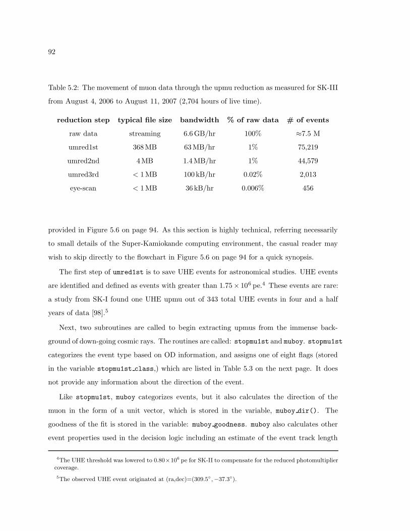
92
Table 5.2: The movement of muon data through the upmu reduction as measured for SK-III
from August 4, 2006 to August 11, 2007 (2,704 hours of live time).
reduction step typical file size bandwidth % of raw data # of events
raw data streaming 6.6GB/hr 100% ≈7.5 M
umred1st 368MB 63MB/hr 1% 75,219
umred2nd 4MB 1.4MB/hr 1% 44,579
umred3rd < 1MB 100 kB/hr 0.02% 2,013
eye-scan < 1MB 36 kB/hr 0.006% 456
provided in Figure 5.6 on page 94. As this section is highly technical, referring necessarily
to small details of the Super-Kamiokande computing environment, the casual reader may
wish to skip directly to the flowchart in Figure 5.6 on page 94 for a quick synopsis.
The first step of umred1st is to save UHE events for astronomical studies. UHE events
are identified and defined as events with greater than 1.75× 10⁶ pe.4 These events are rare:
a study from SK-I found one UHE upmu out of 343 total UHE events in four and a half
years of data [98].5
Next, two subroutines are called to begin extracting upmus from the immense back-
ground of down-going cosmic rays. The routines are called: stopmu1st and muboy. stopmu1st
categorizes the event type based on OD information, and assigns one of eight flags (stored
in the variable stopmu1st class,) which are listed in Table 5.3 on the next page. It does
not provide any information about the direction of the event.
Like stopmu1st, muboy categorizes events, but it also calculates the direction of the
muon in the form of a unit vector, which is stored in the variable, muboy dir(). The
goodness of the fit is stored in the variable: muboy goodness. muboy also calculates other
event properties used in the decision logic including an estimate of the event track length
4The UHE threshold was lowered to 0.80×10⁶ pe for SK-II to compensate for the reduced photomultipliercoverage.
5The observed UHE event originated at (ra,dec)=(309.5,−37.3).
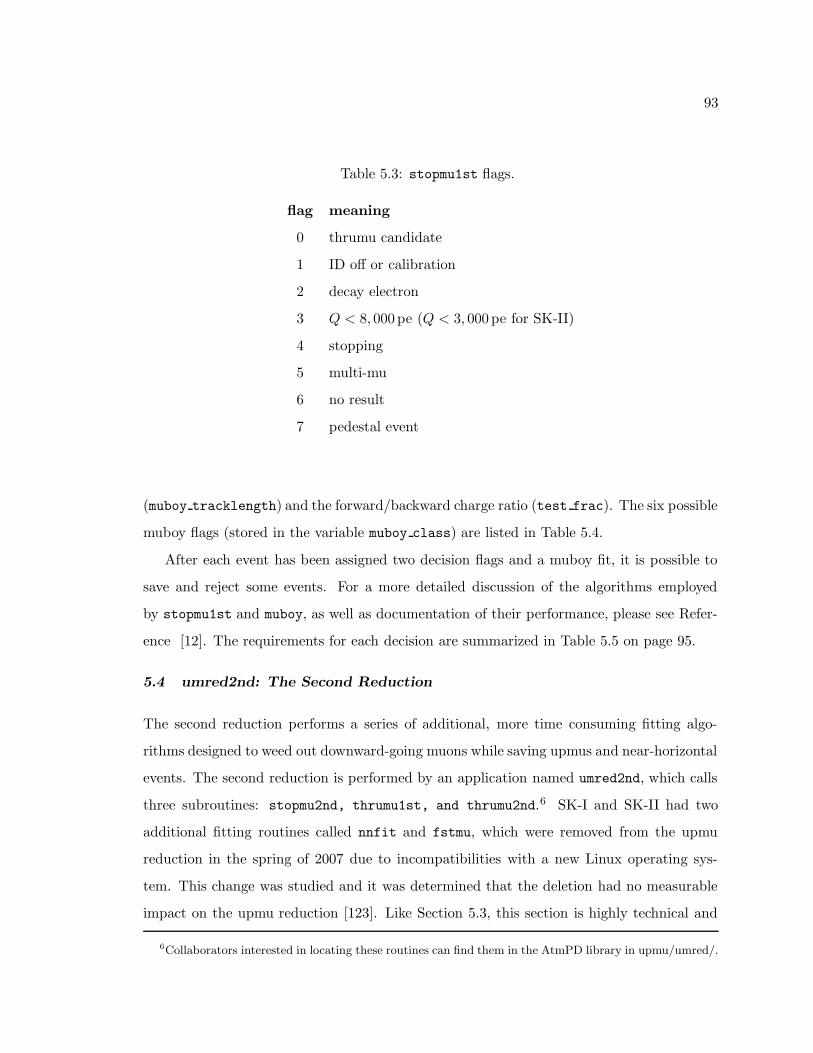
93
Table 5.3: stopmu1st flags.
flag meaning
0 thrumu candidate
1 ID off or calibration
2 decay electron
3 Q < 8, 000 pe (Q < 3, 000 pe for SK-II)
4 stopping
5 multi-mu
6 no result
7 pedestal event
(muboy tracklength) and the forward/backward charge ratio (test frac). The six possible
muboy flags (stored in the variable muboy class) are listed in Table 5.4.
After each event has been assigned two decision flags and a muboy fit, it is possible to
save and reject some events. For a more detailed discussion of the algorithms employed
by stopmu1st and muboy, as well as documentation of their performance, please see Refer-
ence [12]. The requirements for each decision are summarized in Table 5.5 on page 95.
5.4 umred2nd: The Second Reduction
The second reduction performs a series of additional, more time consuming fitting algo-
rithms designed to weed out downward-going muons while saving upmus and near-horizontal
events. The second reduction is performed by an application named umred2nd, which calls
three subroutines: stopmu2nd, thrumu1st, and thrumu2nd.6 SK-I and SK-II had two
additional fitting routines called nnfit and fstmu, which were removed from the upmu
reduction in the spring of 2007 due to incompatibilities with a new Linux operating sys-
tem. This change was studied and it was determined that the deletion had no measurable
impact on the upmu reduction [123]. Like Section 5.3, this section is highly technical and
6Collaborators interested in locating these routines can find them in the AtmPD library in upmu/umred/.
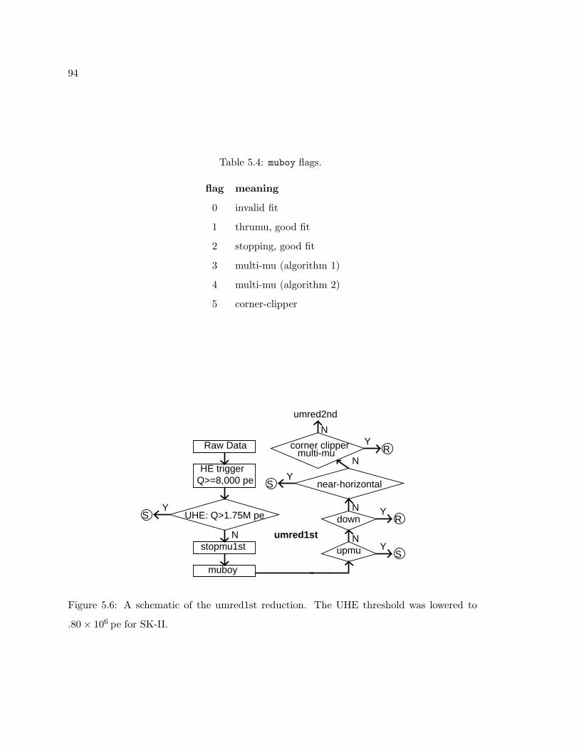
94
Table 5.4: muboy flags.
flag meaning
0 invalid fit
1 thrumu, good fit
2 stopping, good fit
3 multi-mu (algorithm 1)
4 multi-mu (algorithm 2)
5 corner-clipper
Raw Data
HE triggerQ>=8,000 pe
UHE: Q>1.75M peS
stopmu1st upmu
muboy
Y
N
SY
near-horizontal
downY
R
N
N
SY
YR
N
umred2nd
umred1st
corner clippermulti-mu
N
Figure 5.6: A schematic of the umred1st reduction. The UHE threshold was lowered to
.80 × 106 pe for SK-II.
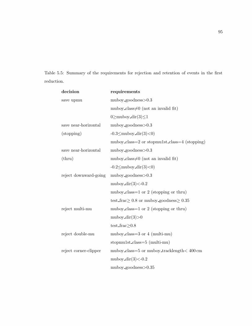
95
Table 5.5: Summary of the requirements for rejection and retention of events in the first
reduction.
decision requirements
save upmu muboy goodness>0.3
muboy class6=0 (not an invalid fit)
0≥muboy dir(3)≤1
save near-horizontal muboy goodness>0.3
(stopping) -0.3≤muboy dir(3)<0)
muboy class=2 or stopmu1st class=4 (stopping)
save near-horizontal muboy goodness>0.3
(thru) muboy class6=0 (not an invalid fit)
-0.2≤muboy dir(3)<0)
reject downward-going muboy goodness>0.3
muboy dir(3)<-0.2
muboy class=1 or 2 (stopping or thru)
test frac≥ 0.8 or muboy goodness≥ 0.35
reject multi-mu muboy class=1 or 2 (stopping or thru)
muboy dir(3)>0
test frac≥0.8
reject double-mu muboy class=3 or 4 (multi-mu)
stopmu1st class=5 (multi-mu)
reject corner-clipper muboy class=5 or muboy tracklength< 400 cm
muboy dir(3)<-0.2
muboy goodness>0.35
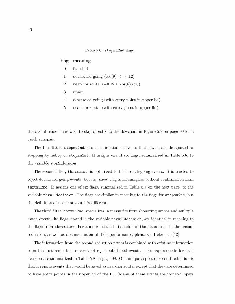
96
Table 5.6: stopmu2nd flags.
flag meaning
0 failed fit
1 downward-going (cos(θ) < −0.12)
2 near-horizontal (−0.12 ≤ cos(θ) < 0)
3 upmu
4 downward-going (with entry point in upper lid)
5 near-horizontal (with entry point in upper lid)
the casual reader may wish to skip directly to the flowchart in Figure 5.7 on page 99 for a
quick synopsis.
The first fitter, stopmu2nd, fits the direction of events that have been designated as
stopping by muboy or stopmu1st. It assigns one of six flags, summarized in Table 5.6, to
the variable stop2 decision.
The second filter, thrumu1st, is optimized to fit through-going events. It is trusted to
reject downward-going events, but its “save” flag is meaningless without confirmation from
thrumu2nd. It assigns one of six flags, summarized in Table 5.7 on the next page, to the
variable thru1 decision. The flags are similar in meaning to the flags for stopmu2nd, but
the definition of near-horizontal is different.
The third filter, thrumu2nd, specializes in messy fits from showering muons and multiple
muon events. Its flags, stored in the variable thru2 decision, are identical in meaning to
the flags from thrumu1st. For a more detailed discussion of the fitters used in the second
reduction, as well as documentation of their performance, please see Reference [12].
The information from the second reduction fitters is combined with existing information
from the first reduction to save and reject additional events. The requirements for each
decision are summarized in Table 5.8 on page 98. One unique aspect of second reduction is
that it rejects events that would be saved as near-horizontal except that they are determined
to have entry points in the upper lid of the ID. (Many of these events are corner-clippers
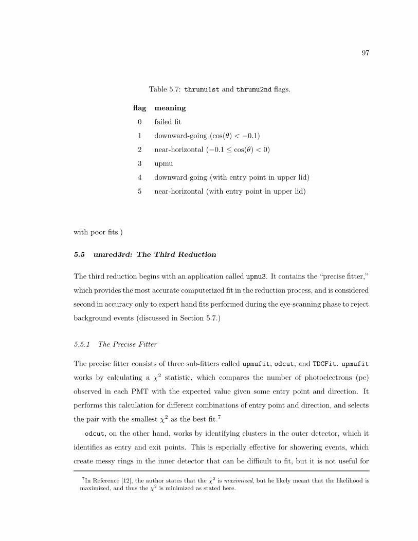
97
Table 5.7: thrumu1st and thrumu2nd flags.
flag meaning
0 failed fit
1 downward-going (cos(θ) < −0.1)
2 near-horizontal (−0.1 ≤ cos(θ) < 0)
3 upmu
4 downward-going (with entry point in upper lid)
5 near-horizontal (with entry point in upper lid)
with poor fits.)
5.5 umred3rd: The Third Reduction
The third reduction begins with an application called upmu3. It contains the “precise fitter,”
which provides the most accurate computerized fit in the reduction process, and is considered
second in accuracy only to expert hand fits performed during the eye-scanning phase to reject
background events (discussed in Section 5.7.)
5.5.1 The Precise Fitter
The precise fitter consists of three sub-fitters called upmufit, odcut, and TDCFit. upmufit
works by calculating a χ2 statistic, which compares the number of photoelectrons (pe)
observed in each PMT with the expected value given some entry point and direction. It
performs this calculation for different combinations of entry point and direction, and selects
the pair with the smallest χ2 as the best fit.7
odcut, on the other hand, works by identifying clusters in the outer detector, which it
identifies as entry and exit points. This is especially effective for showering events, which
create messy rings in the inner detector that can be difficult to fit, but it is not useful for
7In Reference [12], the author states that the χ2 is maximized, but he likely meant that the likelihood ismaximized, and thus the χ2 is minimized as stated here.
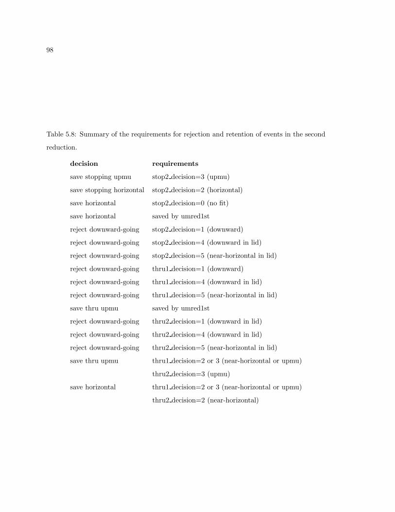
98
Table 5.8: Summary of the requirements for rejection and retention of events in the second
reduction.
decision requirements
save stopping upmu stop2 decision=3 (upmu)
save stopping horizontal stop2 decision=2 (horizontal)
save horizontal stop2 decision=0 (no fit)
save horizontal saved by umred1st
reject downward-going stop2 decision=1 (downward)
reject downward-going stop2 decision=4 (downward in lid)
reject downward-going stop2 decision=5 (near-horizontal in lid)
reject downward-going thru1 decision=1 (downward)
reject downward-going thru1 decision=4 (downward in lid)
reject downward-going thru1 decision=5 (near-horizontal in lid)
save thru upmu saved by umred1st
reject downward-going thru2 decision=1 (downward in lid)
reject downward-going thru2 decision=4 (downward in lid)
reject downward-going thru2 decision=5 (near-horizontal in lid)
save thru upmu thru1 decision=2 or 3 (near-horizontal or upmu)
thru2 decision=3 (upmu)
save horizontal thru1 decision=2 or 3 (near-horizontal or upmu)
thru2 decision=2 (near-horizontal)
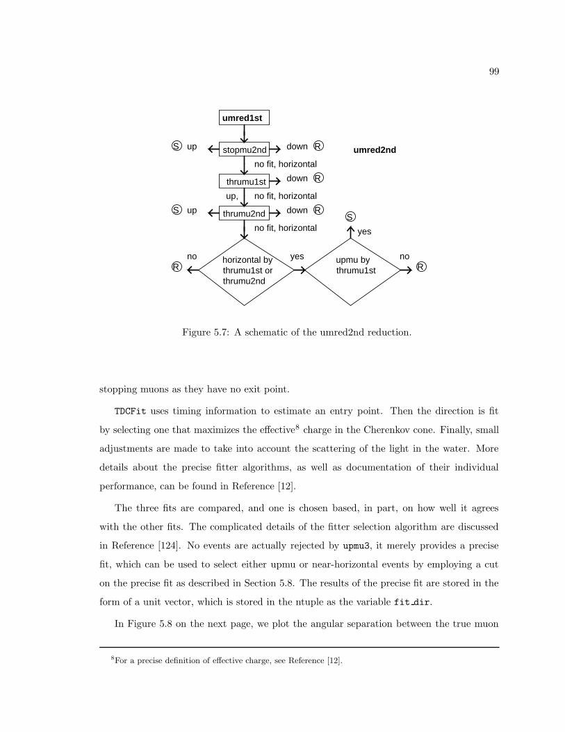
99
stopmu2ndS Rup down
no fit, horizontal
R
RS up
down
down
no fit, horizontal
no fit, horizontal
up,
thrumu1st
noR
yes
yes
noR
S
umred2nd
thrumu2nd
horizontal bythrumu1st orthrumu2nd
upmu bythrumu1st
umred1st
Figure 5.7: A schematic of the umred2nd reduction.
stopping muons as they have no exit point.
TDCFit uses timing information to estimate an entry point. Then the direction is fit
by selecting one that maximizes the effective8 charge in the Cherenkov cone. Finally, small
adjustments are made to take into account the scattering of the light in the water. More
details about the precise fitter algorithms, as well as documentation of their individual
performance, can be found in Reference [12].
The three fits are compared, and one is chosen based, in part, on how well it agrees
with the other fits. The complicated details of the fitter selection algorithm are discussed
in Reference [124]. No events are actually rejected by upmu3, it merely provides a precise
fit, which can be used to select either upmu or near-horizontal events by employing a cut
on the precise fit as described in Section 5.8. The results of the precise fit are stored in the
form of a unit vector, which is stored in the ntuple as the variable fit dir.
In Figure 5.8 on the next page, we plot the angular separation between the true muon
8For a precise definition of effective charge, see Reference [12].
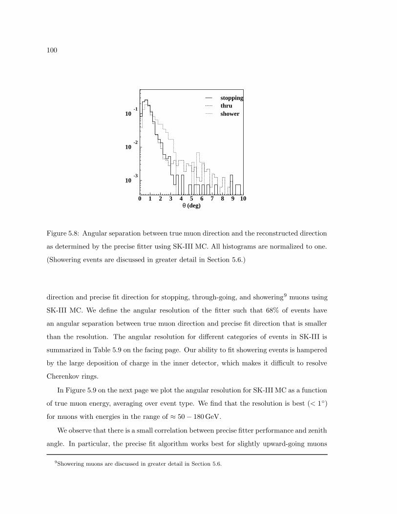
100
θ (deg)
stoppingthrushower
10-3
10-2
10-1
0 1 2 3 4 5 6 7 8 9 10
Figure 5.8: Angular separation between true muon direction and the reconstructed direction
as determined by the precise fitter using SK-III MC. All histograms are normalized to one.
(Showering events are discussed in greater detail in Section 5.6.)
direction and precise fit direction for stopping, through-going, and showering9 muons using
SK-III MC. We define the angular resolution of the fitter such that 68% of events have
an angular separation between true muon direction and precise fit direction that is smaller
than the resolution. The angular resolution for different categories of events in SK-III is
summarized in Table 5.9 on the facing page. Our ability to fit showering events is hampered
by the large deposition of charge in the inner detector, which makes it difficult to resolve
Cherenkov rings.
In Figure 5.9 on the next page we plot the angular resolution for SK-III MC as a function
of true muon energy, averaging over event type. We find that the resolution is best (< 1)
for muons with energies in the range of ≈ 50 − 180GeV.
We observe that there is a small correlation between precise fitter performance and zenith
angle. In particular, the precise fit algorithm works best for slightly upward-going muons
9Showering muons are discussed in greater detail in Section 5.6.
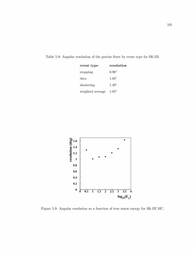
101
Table 5.9: Angular resolution of the precise fitter by event type for SK-III.
event type resolution
stopping 0.96
thru 1.05
showering 1.40
weighted average 1.05
0
0.2
0.4
0.6
0.8
1
1.2
1.4
1.6
0 0.5 1 1.5 2 2.5 3 3.5 4
log10(Eµ)
reso
luti
on (
deg)
Figure 5.9: Angular resolution as a function of true muon energy for SK-III MC.
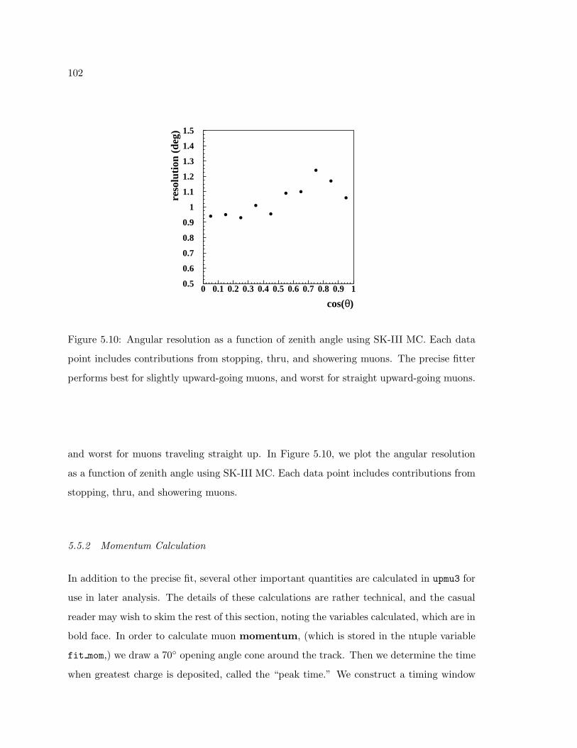
102
cos(θ)
reso
luti
on (
deg)
0.5
0.6
0.7
0.8
0.9
1
1.1
1.2
1.3
1.4
1.5
0 0.1 0.2 0.3 0.4 0.5 0.6 0.7 0.8 0.9 1
Figure 5.10: Angular resolution as a function of zenith angle using SK-III MC. Each data
point includes contributions from stopping, thru, and showering muons. The precise fitter
performs best for slightly upward-going muons, and worst for straight upward-going muons.
and worst for muons traveling straight up. In Figure 5.10, we plot the angular resolution
as a function of zenith angle using SK-III MC. Each data point includes contributions from
stopping, thru, and showering muons.
5.5.2 Momentum Calculation
In addition to the precise fit, several other important quantities are calculated in upmu3 for
use in later analysis. The details of these calculations are rather technical, and the casual
reader may wish to skim the rest of this section, noting the variables calculated, which are in
bold face. In order to calculate muon momentum, (which is stored in the ntuple variable
fit mom,) we draw a 70 opening angle cone around the track. Then we determine the time
when greatest charge is deposited, called the “peak time.” We construct a timing window
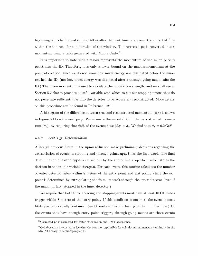
103
beginning 50 ns before and ending 250 ns after the peak time, and count the corrected10 pe
within the the cone for the duration of the window. The corrected pe is converted into a
momentum using a table generated with Monte Carlo.11
It is important to note that fit mom represents the momentum of the muon once it
penetrates the ID. Therefore, it is only a lower bound on the muon’s momentum at the
point of creation, since we do not know how much energy was dissipated before the muon
reached the ID, (nor how much energy was dissipated after a through-going muon exits the
ID.) The muon momentum is used to calculate the muon’s track length, and we shall see in
Section 5.7 that it provides a useful variable with which to cut out stopping muons that do
not penetrate sufficiently far into the detector to be accurately reconstructed. More details
on this procedure can be found in Reference [125].
A histogram of the difference between true and reconstructed momentum (∆p) is shown
in Figure 5.11 on the next page. We estimate the uncertainty in the reconstructed momen-
tum (σp), by requiring that 68% of the events have |∆p| < σp We find that σp = 0.2GeV.
5.5.3 Event Type Determination
Although previous filters in the upmu reduction make preliminary decisions regarding the
categoriation of events as stopping and through-going, upmu3 has the final word. The final
determination of event type is carried out by the subroutine stop thru, which stores the
decision in the ntuple variable fit pid. For each event, this routine calculates the number
of outer detector tubes within 8 meters of the entry point and exit point, where the exit
point is determined by extrapolating the fit muon track through the outer detector (even if
the muon, in fact, stopped in the inner detector.)
We require that both through-going and stopping events must have at least 10 OD tubes
trigger within 8 meters of the entry point. If this condition is not met, the event is most
likely partially or fully contained, (and therefore does not belong in the upmu sample.) Of
the events that have enough entry point triggers, through-going muons are those events
10Corrected pe is corrected for water attenuation and PMT acceptance.
11Collaborators interested in locating the routine responsible for calculating momentum can find it in theAtmPD library in seplib/sprngsep.F.
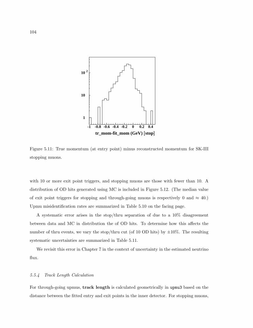
104
tr_mom-fit_mom (GeV) [stop]
1
10
10 2
-1 -0.8 -0.6 -0.4 -0.2 0 0.2 0.4
Figure 5.11: True momentum (at entry point) minus reconstructed momentum for SK-III
stopping muons.
with 10 or more exit point triggers, and stopping muons are those with fewer than 10. A
distribution of OD hits generated using MC is included in Figure 5.12. (The median value
of exit point triggers for stopping and through-going muons is respectively 0 and ≈ 40.)
Upmu misidentification rates are summarized in Table 5.10 on the facing page.
A systematic error arises in the stop/thru separation of due to a 10% disagreement
between data and MC in distribution the of OD hits. To determine how this affects the
number of thru events, we vary the stop/thru cut (of 10 OD hits) by ±10%. The resulting
systematic uncertainties are summarized in Table 5.11.
We revisit this error in Chapter 7 in the context of uncertainty in the estimated neutrino
flux.
5.5.4 Track Length Calculation
For through-going upmus, track length is calculated geometrically in upmu3 based on the
distance between the fitted entry and exit points in the inner detector. For stopping muons,
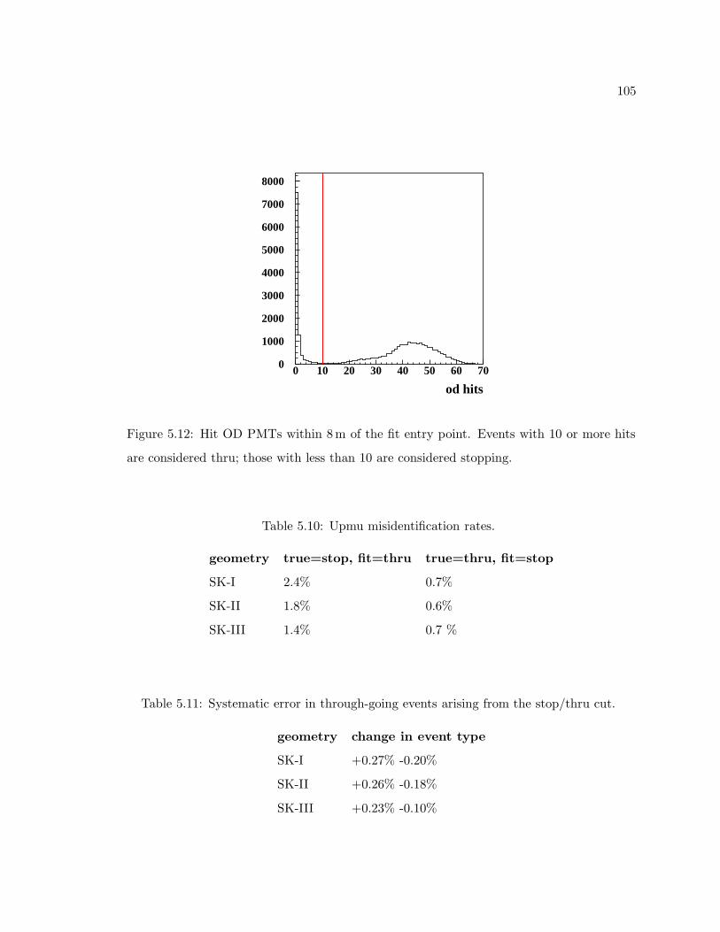
105
od hits
0
1000
2000
3000
4000
5000
6000
7000
8000
0 10 20 30 40 50 60 70
Figure 5.12: Hit OD PMTs within 8m of the fit entry point. Events with 10 or more hits
are considered thru; those with less than 10 are considered stopping.
Table 5.10: Upmu misidentification rates.
geometry true=stop, fit=thru true=thru, fit=stop
SK-I 2.4% 0.7%
SK-II 1.8% 0.6%
SK-III 1.4% 0.7 %
Table 5.11: Systematic error in through-going events arising from the stop/thru cut.
geometry change in event type
SK-I +0.27% -0.20%
SK-II +0.26% -0.18%
SK-III +0.23% -0.10%
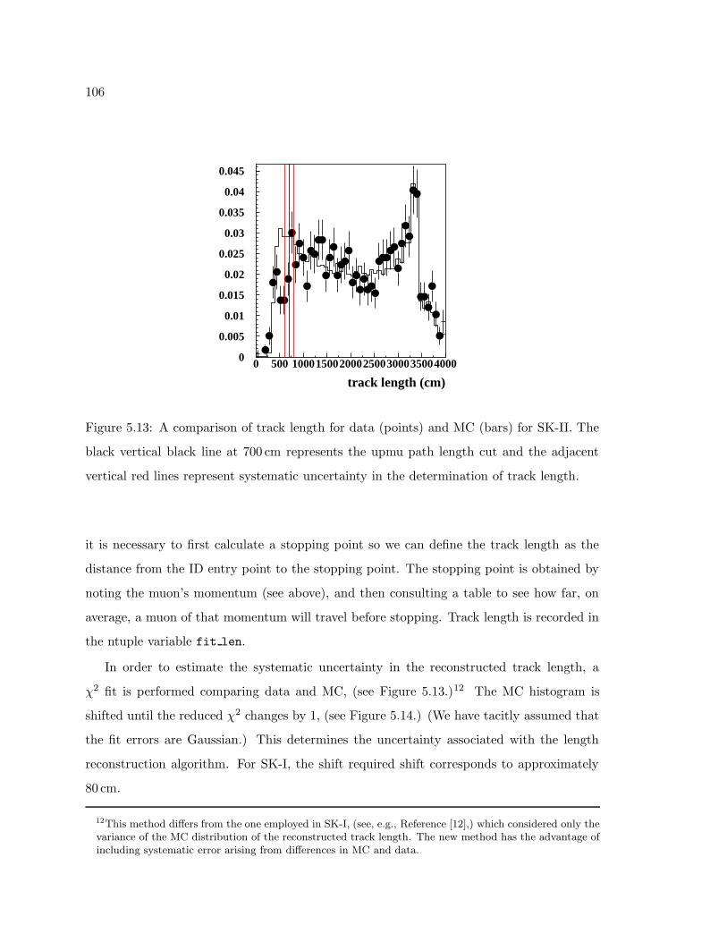
106
track length (cm)
0
0.005
0.01
0.015
0.02
0.025
0.03
0.035
0.04
0.045
0 500 1000150020002500300035004000
Figure 5.13: A comparison of track length for data (points) and MC (bars) for SK-II. The
black vertical black line at 700 cm represents the upmu path length cut and the adjacent
vertical red lines represent systematic uncertainty in the determination of track length.
it is necessary to first calculate a stopping point so we can define the track length as the
distance from the ID entry point to the stopping point. The stopping point is obtained by
noting the muon’s momentum (see above), and then consulting a table to see how far, on
average, a muon of that momentum will travel before stopping. Track length is recorded in
the ntuple variable fit len.
In order to estimate the systematic uncertainty in the reconstructed track length, a
χ2 fit is performed comparing data and MC, (see Figure 5.13.)12 The MC histogram is
shifted until the reduced χ2 changes by 1, (see Figure 5.14.) (We have tacitly assumed that
the fit errors are Gaussian.) This determines the uncertainty associated with the length
reconstruction algorithm. For SK-I, the shift required shift corresponds to approximately
80 cm.
12This method differs from the one employed in SK-I, (see, e.g., Reference [12],) which considered only thevariance of the MC distribution of the reconstructed track length. The new method has the advantage ofincluding systematic error arising from differences in MC and data.
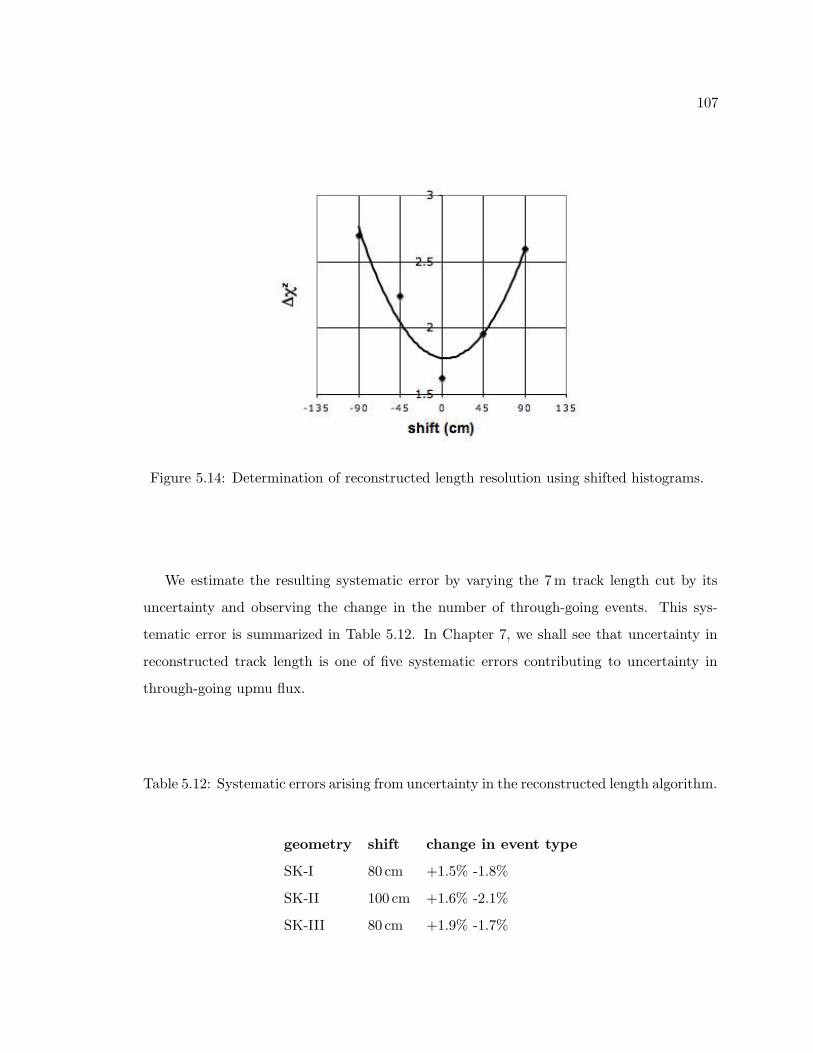
107
Figure 5.14: Determination of reconstructed length resolution using shifted histograms.
We estimate the resulting systematic error by varying the 7m track length cut by its
uncertainty and observing the change in the number of through-going events. This sys-
tematic error is summarized in Table 5.12. In Chapter 7, we shall see that uncertainty in
reconstructed track length is one of five systematic errors contributing to uncertainty in
through-going upmu flux.
Table 5.12: Systematic errors arising from uncertainty in the reconstructed length algorithm.
geometry shift change in event type
SK-I 80 cm +1.5% -1.8%
SK-II 100 cm +1.6% -2.1%
SK-III 80 cm +1.9% -1.7%
108
5.6 Showering Muons
In Reference [12], an algorithm was developed for separating the through-going muon sample
into showering events with a peak neutrino energy of 800 GeV and non-showering events with
a peak neutrino energy of 100 GeV, (see Figure 5.3 on page 89 for energy distributions of the
different types of events.) We have now incorporated the showering algorithm into upmu3.
Throughout this work we shorten “through-going non-showering muons” to “through-going
muons” and “through-going showering” to “showering” in contexts where there is a dis-
tinction to be made between showering and non-showering muons. Thus, through-going
muons and showering muons are topologically distinct sets, even though showering muons
are considered through-going before we apply the showering algorithm.
The strategy behind the showering algorithm is to take advantage of the fact that muons
with modest energies deposit charge primarily through ionization (at a steady rate of ≈2.2MeV/cm in water,) whereas very high-energy muons are prone to sudden catastrophic
energy loss due to pair production, Bremsstrahlung, and photonuclear interactions. At
≈ 1TeV, muon energy loss per unit track length from showering mechanisms becomes equal
to that from ionization, (see Figure 5.15 on the facing page.)
The algorithm defines a χ2 statistic, which compares the corrected charge deposited
over consecutive 50 cm intervals of track (Qicorr) with the corrected charge averaged over
the track (〈Qcorr〉)—the idea being that ionization deposits charge with near uniformity in
time whereas showering is associated with sudden deposition of energy. It also compares the
corrected charge averaged over the track with the expected value for non-showering muons:
Q(l), which is a function of track length. The resulting statistic is of the following form:
χ2 =
N−2∑
i=3
[Qicorr − 〈Qcorr〉]2
σ2qi
+[〈Qcorr〉 −Q(l)]2
σ2Q(l)
, |Qicorr −Q(l)| ≥ −2 (5.1)
σQicorr
and σ2Q(l) are the statistical errors in Qi
corr and Q(l) respectively. The bounds of the
sum are chosen to be at least a meter from the walls where it is hard to characterize the
corrected charge. The sum only includes terms whereQicorr−Q(l) ≥ −2, which correspond to
fluctuations above the expected charge deposition from non-showering muons. An additional
showering variable, (defined as ∆, but sometimes referred to as “diff,”) is defined to identify
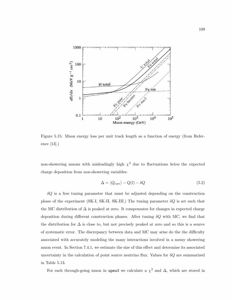
109
Figure 5.15: Muon energy loss per unit track length as a function of energy (from Refer-
ence [13].)
non-showering muons with misleadingly high χ2 due to fluctuations below the expected
charge deposition from non-showering variables:
∆ = 〈Qcorr〉 −Q(l) − δQ (5.2)
δQ is a free tuning parameter that must be adjusted depending on the construction
phase of the experiment (SK-I, SK-II, SK-III.) The tuning parameter δQ is set such that
the MC distribution of ∆ is peaked at zero. It compensates for changes in expected charge
deposition during different construction phases. After tuning δQ with MC, we find that
the distribution for ∆ is close to, but not precisely peaked at zero and so this is a source
of systematic error. The discrepancy between data and MC may arise do the the difficulty
associated with accurately modeling the many interactions involved in a messy showering
muon event. In Section 7.4.1, we estimate the size of this effect and determine its associated
uncertainty in the calculation of point source neutrino flux. Values for δQ are summarized
in Table 5.13.
For each through-going muon in upmu3 we calculate a χ2 and ∆, which are stored in
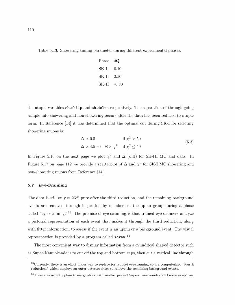
110
Table 5.13: Showering tuning parameter during different experimental phases.
Phase δQ
SK-I 0.10
SK-II 2.50
SK-II -0.30
the ntuple variables sh chi1p and sh delta respectively. The separation of through-going
sample into showering and non-showering occurs after the data has been reduced to ntuple
form. In Reference [14] it was determined that the optimal cut during SK-I for selecting
showering muons is:
∆ > 0.5 if χ2 > 50
∆ > 4.5 − 0.08 × χ2 if χ2 ≤ 50(5.3)
In Figure 5.16 on the next page we plot χ2 and ∆ (diff) for SK-III MC and data. In
Figure 5.17 on page 112 we provide a scatterplot of ∆ and χ2 for SK-I MC showering and
non-showering muons from Reference [14].
5.7 Eye-Scanning
The data is still only ≈ 23% pure after the third reduction, and the remaining background
events are removed through inspection by members of the upmu group during a phase
called “eye-scanning.”13 The premise of eye-scanning is that trained eye-scanners analyze
a pictorial representation of each event that makes it through the third reduction, along
with fitter information, to assess if the event is an upmu or a background event. The visual
representation is provided by a program called idraw.14
The most convenient way to display information from a cylindrical shaped detector such
as Super-Kamiokande is to cut off the top and bottom caps, then cut a vertical line through
13Currently, there is an effort under way to replace (or reduce) eye-scanning with a computerized “fourthreduction,” which employs an outer detector fitter to remove the remaining background events.
14There are currently plans to merge idraw with another piece of Super-Kamiokande code known as apdraw.
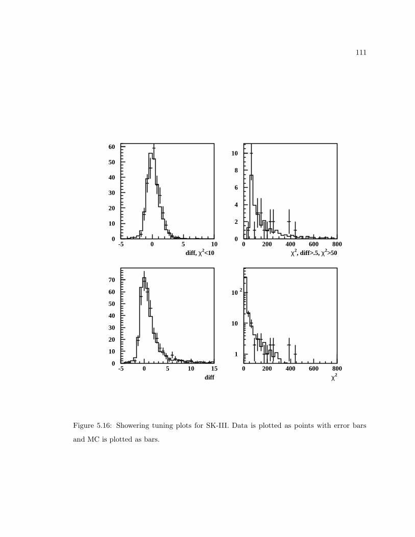
111
0
10
20
30
40
50
60
-5 0 5 100
2
4
6
8
10
0 200 400 600 800
0
10
20
30
40
50
60
70
-5 0 5 10 15
diff, χ2<10 χ2, diff>.5, χ2>50
diff χ2
1
10
10 2
0 200 400 600 800
Figure 5.16: Showering tuning plots for SK-III. Data is plotted as points with error bars
and MC is plotted as bars.
112
Figure 5.17: A scatterplot of ∆ and χ2 for SK-I MC showering (left) and non-showering
muons (right) from Reference [14].
the barrel, and unroll it into a flat rectangular sheet. An example of such a representation
is shown in Figure 5.18 on the next page, which depicts a multi-mu event. The large display
represents the unfolded ID and the smaller version in the upper left-hand corner represents
the OD. Bigger circles indicate greater charge deposition and the precise fit is indicated
with a solid red line. Entry and exit points are marked with asterisks. (The dashed line is
the muboy fit.) Even the untrained eye can see that the precise fit does match well with the
deposition of charge, which is one of several indicators that this is a background event. The
large deposition of charge is consistent with a multi-mu hypothesis.
There are four pieces of information that an eye-scanner can use in deciding to save or
reject a fit. They include: the quality of the fit, entry and/or sometimes exit clusters
in the OD, timing information, and manual fits. When downward-going multi-mus
and corner-clippers trick the precise fitter into producing an upward-going fit, it is usually
obvious (to a person looking at an event display) that the precise fit does not align with the
edges of the Cherenkov ring. The fitter is particularly prone to mistakes when the track is
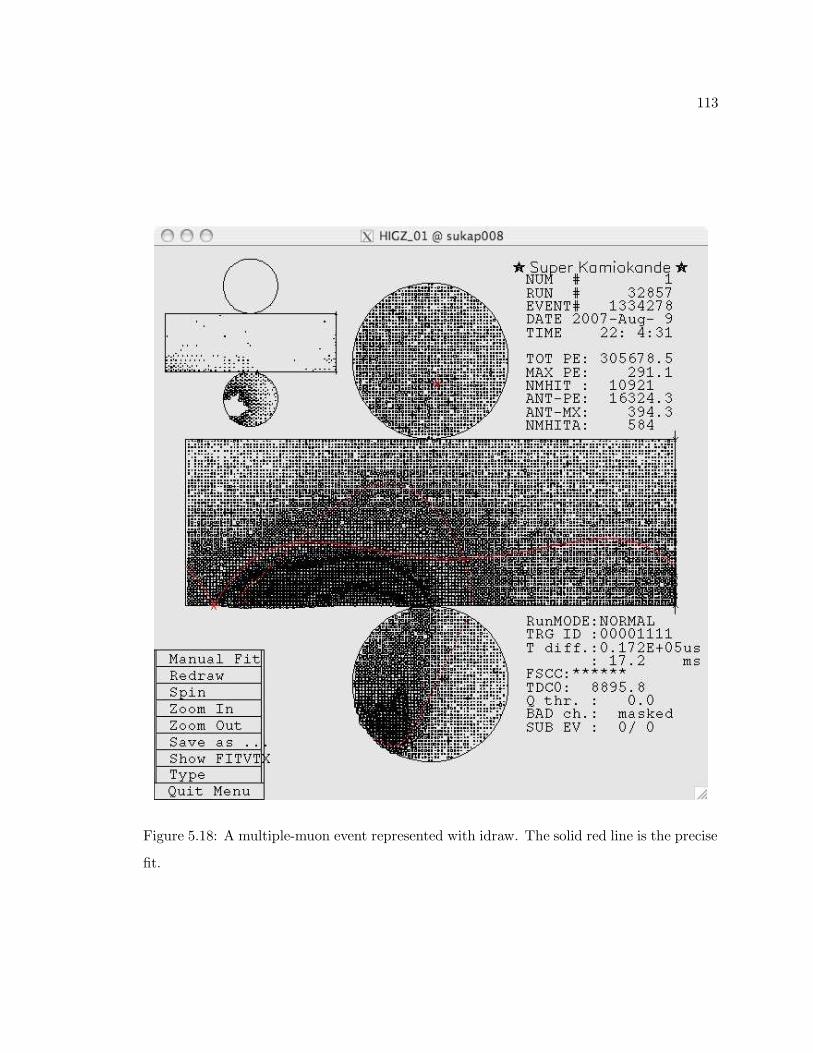
113
Figure 5.18: A multiple-muon event represented with idraw. The solid red line is the precise
fit.
114
near the edge of the detector (corner-clippers) and when there is a large amount of charge
deposited in the ID (multi-mus and showering down-mus,) but humans are adept at pattern
recognition and can quickly identify these events.
Often through-going events will leave clustering in the OD. Eye-scanners are trained
to look for such clusters in the OD to find evidence in support of an upmu or down-
mu hypothesis. This is especially useful when a showering event deposits a large amount
of charge in the ID, making reconstruction difficult. Timing information is often used
in conjunction with OD clusters. Eye-scanners have the option of displaying color-coded
timing information, where early PMT triggers are red and late PMT triggers are blue. By
determining which PMTs are hit first, eye-scanners can test the likelihood of a hypothesized
muon direction.
Finally, eye-scanners have the option of performing a manual fit. This can be useful
when the precise fit is close, but visibly off. It is also useful for testing the plausibility of
certain scenarios: e.g., Could that pattern on the lower cap be produced by a muon entering
here? When performing a manual fit, the eye-scanner selects hypothesized entry and exit
points, and idraw calculates the Cherenkov ring based on the fit mom variable discussed in
Section 5.5, superimposing the results of the manual fit on the event display. If a manual
fit finds an event to be downward and the direction is found to be greater than 5 from the
precise fitter direction, the event is rejected. A manual fit that differs by less than 5 from
the precise fit is saved even if it finds the muon to be downward-going. In no circumstance
does the manual fit replace the precise fit; it is only used to save/reject events.
All events are scanned independently by two trained scanners. Training consists of a
tutorial and a practice scan of a sample of pre-scanned events with known answers. For
each event, scanners have the option of saving the event, rejecting the event, or they may
declare that they are uncertain. If an event is rejected, a note is recorded explaining why.
If there is a disagreement between two scanners, or if one or both scanners are uncertain,
the event is passed to an expert scanner.
Expert scanners have participated in eye-scanning during past upmu reductions. For the
SK-III upmu reduction, the expert scanners were myself and Jen Raaf. Past studies [16] have
determined the mean angular difference in manual fits, performed by two different scanners
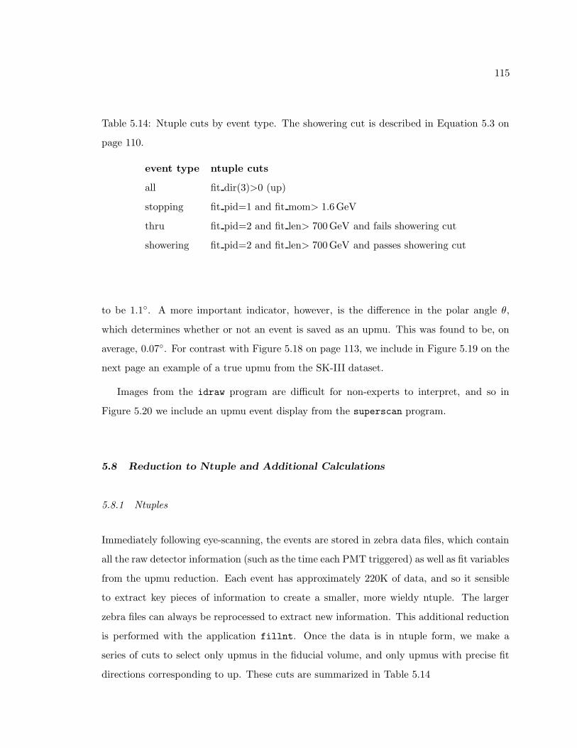
115
Table 5.14: Ntuple cuts by event type. The showering cut is described in Equation 5.3 on
page 110.
event type ntuple cuts
all fit dir(3)>0 (up)
stopping fit pid=1 and fit mom> 1.6GeV
thru fit pid=2 and fit len> 700GeV and fails showering cut
showering fit pid=2 and fit len> 700GeV and passes showering cut
to be 1.1. A more important indicator, however, is the difference in the polar angle θ,
which determines whether or not an event is saved as an upmu. This was found to be, on
average, 0.07. For contrast with Figure 5.18 on page 113, we include in Figure 5.19 on the
next page an example of a true upmu from the SK-III dataset.
Images from the idraw program are difficult for non-experts to interpret, and so in
Figure 5.20 we include an upmu event display from the superscan program.
5.8 Reduction to Ntuple and Additional Calculations
5.8.1 Ntuples
Immediately following eye-scanning, the events are stored in zebra data files, which contain
all the raw detector information (such as the time each PMT triggered) as well as fit variables
from the upmu reduction. Each event has approximately 220K of data, and so it sensible
to extract key pieces of information to create a smaller, more wieldy ntuple. The larger
zebra files can always be reprocessed to extract new information. This additional reduction
is performed with the application fillnt. Once the data is in ntuple form, we make a
series of cuts to select only upmus in the fiducial volume, and only upmus with precise fit
directions corresponding to up. These cuts are summarized in Table 5.14
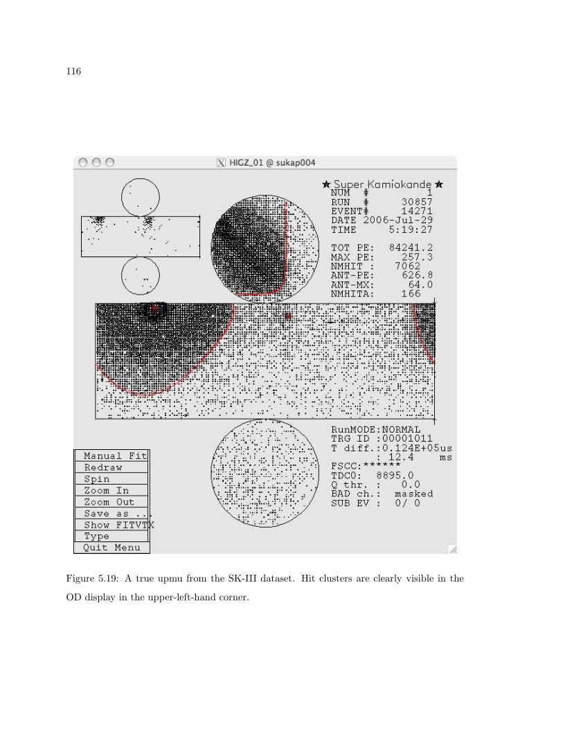
116
Figure 5.19: A true upmu from the SK-III dataset. Hit clusters are clearly visible in the
OD display in the upper-left-hand corner.
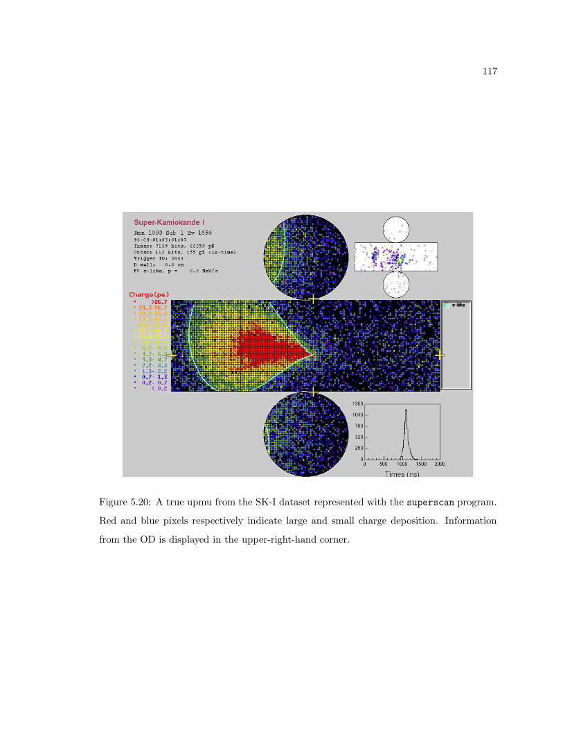
117
Figure 5.20: A true upmu from the SK-I dataset represented with the superscan program.
Red and blue pixels respectively indicate large and small charge deposition. Information
from the OD is displayed in the upper-right-hand corner.
118
5.8.2 Live Time Calculation
After reducing the data to ntuple, it is necessary to compute the experiment’s live time.
Live time is a key ingredient in the calculation of flux as well as astronomical exposure time,
(the duration for which the detector is sensitive to upmu-inducing neutrinos from different
equatorial coordinates.) During the first year of SK-III, Super-Kamiokande operated with
a duty cycle of 31%. SK-I, by contrast, operated with a duty cycle of 90% [12]. (The low
duty cycle for SK-III thus far is likely due to increased calibration and maintenance work
immediately following the rebuild.) Every event is time-stamped with a GPS time that is
accurate to within 20 ns, and we use these time-stamps to determine the live time.
Maintenance work, where the detector is temporarily shut down, is a source of downtime,
which tends to diminish in frequency as detector performance stabilizes. There are several
other sources of “dead time,” however, where the detector is operating, but is in some way
incapacitated, and can not take data. Dead time, is a permanent feature of the experiment,
and does not diminish in frequency with time. The sources of dead time can be understood
as three general categories: busy in progress (BIP), hardware malfunction, and calibration.
BIP dead time occurs when there are two high-energy triggers within 8 − 56µs of
each other. The 8 − 56µs range reflects the fact that some very energetic events take a
long time to save, whereas simpler lower energy events can be saved quickly. Starting 6µs
after a high-energy trigger, and lasting for up to 50µs the TDCs are busy saving data from
the past event and are unable to record additional events [111]. If additional high-energy
triggers occur during this window, the triggers themselves are recorded with a time-stamp,
but the details of the event, (i.e., charge and timing information for each PMT,) are lost,
and the event is considered “dead.” Dead triggers are not removed from the data stream
as they are used for calculating dead time. Once the TDC is finished saving data, the next
trigger will be recorded as live.
We define live time as follows. The time after a live event and a subsequent dead event is
recorded as dead time. Time between consecutive dead events is also recorded as dead time.
The time after a dead event and a consecutive live event is live time, as is the time between
two live events. This definition of dead time takes advantage of the fact that we continue
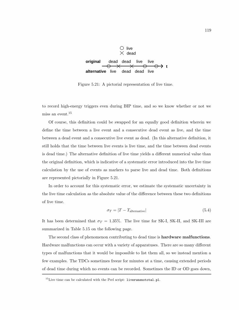
119
dead livedead live
deaddead livelive
original
alternative
deadlive
t
Figure 5.21: A pictorial representation of live time.
to record high-energy triggers even during BIP time, and so we know whether or not we
miss an event.15
Of course, this definition could be swapped for an equally good definition wherein we
define the time between a live event and a consecutive dead event as live, and the time
between a dead event and a consecutive live event as dead. (In this alternative definition, it
still holds that the time between live events is live time, and the time between dead events
is dead time.) The alternative definition of live time yields a different numerical value than
the original definition, which is indicative of a systematic error introduced into the live time
calculation by the use of events as markers to parse live and dead time. Both definitions
are represented pictorially in Figure 5.21.
In order to account for this systematic error, we estimate the systematic uncertainty in
the live time calculation as the absolute value of the difference between these two definitions
of live time.
σT = |T − Talternative| (5.4)
It has been determined that σT = 1.35%. The live time for SK-I, SK-II, and SK-III are
summarized in Table 5.15 on the following page.
The second class of phenomenon contributing to dead time is hardware malfunctions.
Hardware malfunctions can occur with a variety of apparatuses. There are so many different
types of malfunctions that it would be impossible to list them all, so we instead mention a
few examples. The TDCs sometimes freeze for minutes at a time, causing extended periods
of dead time during which no events can be recorded. Sometimes the ID or OD goes down,
15Live time can be calculated with the Perl script: liverunsnototal.pl.
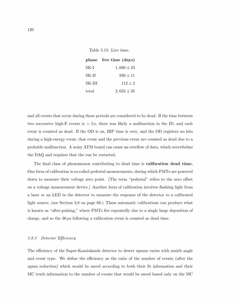
120
Table 5.15: Live time.
phase live time (days)
SK-I 1, 680 ± 23
SK-II 830 ± 11
SK-III 112 ± 2
total 2, 623 ± 35
and all events that occur during these periods are considered to be dead. If the time between
two successive high-E events is > 5 s, there was likely a malfunction in the ID, and each
event is counted as dead. If the OD is on, BIP time is over, and the OD registers no hits
during a high-energy event, that event and the previous event are counted as dead due to a
probable malfunction. A noisy ATM board can cause an overflow of data, which overwhelms
the DAQ and requires that the run be restarted.
The final class of phenomenon contributing to dead time is calibration dead time.
One form of calibration is so-called pedestal measurements, during which PMTs are powered
down to measure their voltage zero point. (The term “pedestal” refers to the zero offset
on a voltage measurement device.) Another form of calibration involves flashing light from
a laser or an LED in the detector to measure the response of the detector to a calibrated
light source, (see Section 3.8 on page 68.) These automatic calibrations can produce what
is known as “after-pulsing,” where PMTs fire repeatedly due to a single large deposition of
charge, and so the 30µs following a calibration event is counted as dead time.
5.8.3 Detector Efficiency
The efficiency of the Super-Kamiokande detector to detect upmus varies with zenith angle
and event type. We define the efficiency as the ratio of the number of events (after the
upmu reduction) which would be saved according to both their fit information and their
MC truth information to the number of events that would be saved based only on the MC
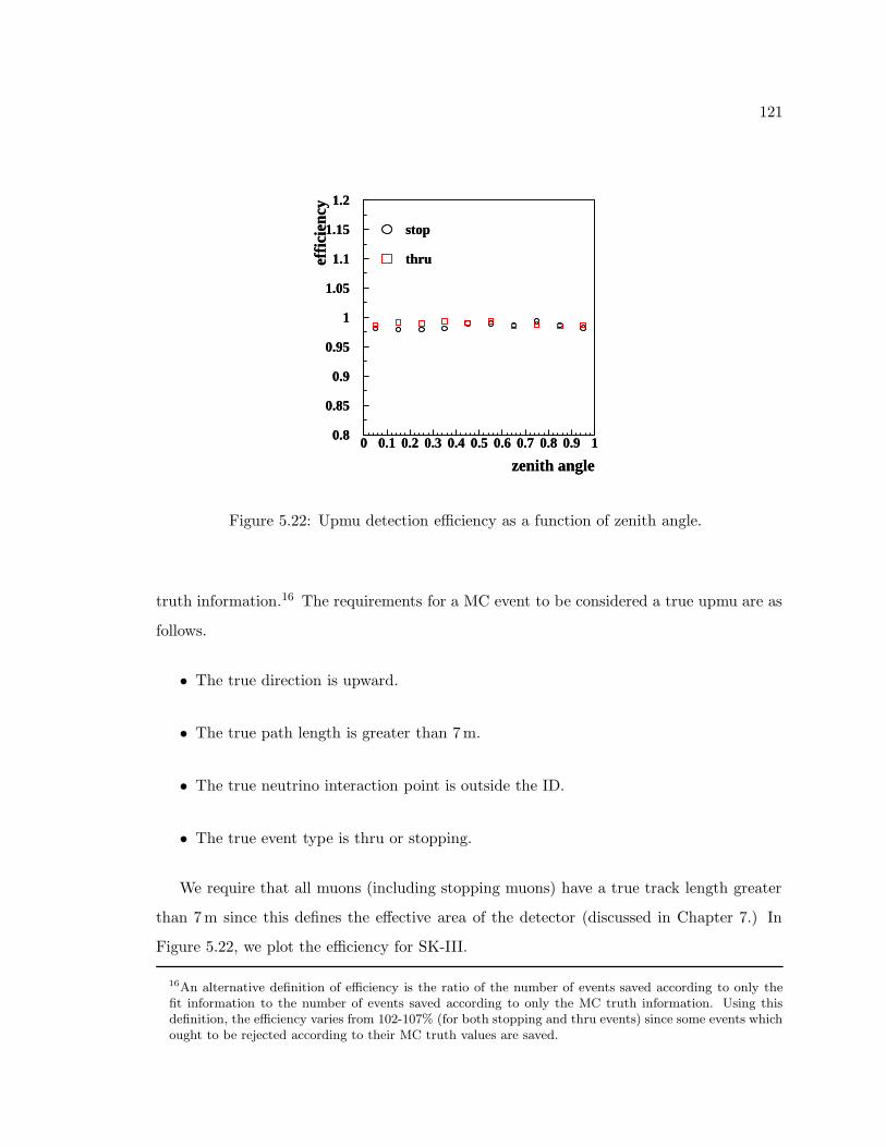
121
0.8
0.85
0.9
0.95
1
1.05
1.1
1.15
1.2
0 0.1 0.2 0.3 0.4 0.5 0.6 0.7 0.8 0.9 1
stop
thru
zenith angle
effi
cien
cy
stop
thru
zenith angle
effi
cien
cy
0.8
0.85
0.9
0.95
1
1.05
1.1
1.15
1.2
0 0.1 0.2 0.3 0.4 0.5 0.6 0.7 0.8 0.9 1
Figure 5.22: Upmu detection efficiency as a function of zenith angle.
truth information.16 The requirements for a MC event to be considered a true upmu are as
follows.
• The true direction is upward.
• The true path length is greater than 7m.
• The true neutrino interaction point is outside the ID.
• The true event type is thru or stopping.
We require that all muons (including stopping muons) have a true track length greater
than 7m since this defines the effective area of the detector (discussed in Chapter 7.) In
Figure 5.22, we plot the efficiency for SK-III.
16An alternative definition of efficiency is the ratio of the number of events saved according to only thefit information to the number of events saved according to only the MC truth information. Using thisdefinition, the efficiency varies from 102-107% (for both stopping and thru events) since some events whichought to be rejected according to their MC truth values are saved.
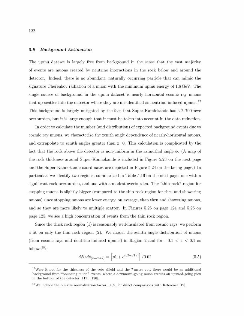
122
5.9 Background Estimation
The upmu dataset is largely free from background in the sense that the vast majority
of events are muons created by neutrino interactions in the rock below and around the
detector. Indeed, there is no abundant, naturally occurring particle that can mimic the
signature Cherenkov radiation of a muon with the minimum upmu energy of 1.6GeV. The
single source of background in the upmu dataset is nearly horizontal cosmic ray muons
that up-scatter into the detector where they are misidentified as neutrino-induced upmus.17
This background is largely mitigated by the fact that Super-Kamiokande has a 2, 700mwe
overburden, but it is large enough that it must be taken into account in the data reduction.
In order to calculate the number (and distribution) of expected background events due to
cosmic ray muons, we characterize the zenith angle dependence of nearly-horizontal muons,
and extrapolate to zenith angles greater than z=0. This calculation is complicated by the
fact that the rock above the detector is non-uniform in the azimuthal angle φ. (A map of
the rock thickness around Super-Kamiokande is included in Figure 5.23 on the next page
and the Super-Kamiokande coordinates are depicted in Figure 5.24 on the facing page.) In
particular, we identify two regions, summarized in Table 5.16 on the next page; one with a
significant rock overburden, and one with a modest overburden. The “thin rock” region for
stopping muons is slightly bigger (compared to the thin rock region for thru and showering
muons) since stopping muons are lower energy, on average, than thru and showering muons,
and so they are more likely to multiple scatter. In Figures 5.25 on page 124 and 5.26 on
page 125, we see a high concentration of events from the thin rock region.
Since the thick rock region (1) is reasonably well-insulated from cosmic rays, we perform
a fit on only the thin rock region (2). We model the zenith angle distribution of muons
(from cosmic rays and neutrino-induced upmus) in Region 2 and for −0.1 < z < 0.1 as
follows18:
dN/dz(z=cos θ) =[
p1 + e(p2−p3 z)]
/0.02 (5.5)
17Were it not for the thickness of the veto shield and the 7 meter cut, there would be an additionalbackground from “bouncing muon” events, where a downward-going muon creates an upward-going pionin the bottom of the detector [117], [126].
18We include the bin size normalization factor, 0.02, for direct comparisons with Reference [12].
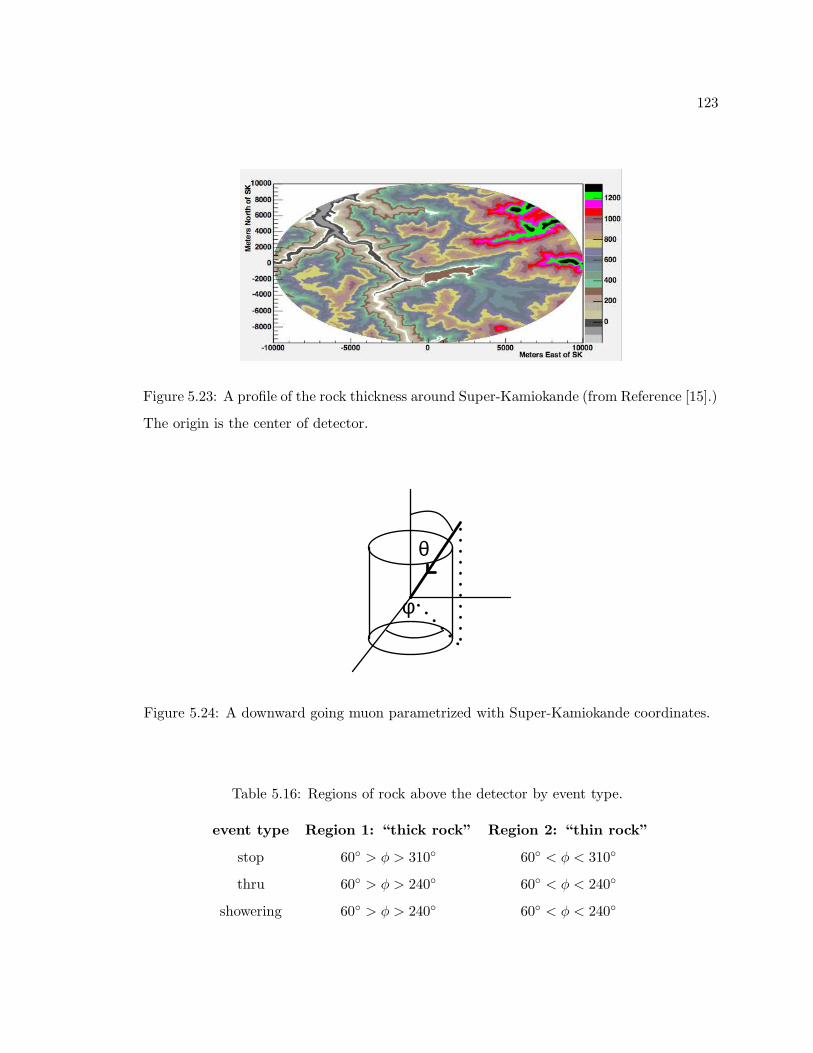
123
Figure 5.23: A profile of the rock thickness around Super-Kamiokande (from Reference [15].)
The origin is the center of detector.
θ
φ
Figure 5.24: A downward going muon parametrized with Super-Kamiokande coordinates.
Table 5.16: Regions of rock above the detector by event type.
event type Region 1: “thick rock” Region 2: “thin rock”
stop 60 > φ > 310 60 < φ < 310
thru 60 > φ > 240 60 < φ < 240
showering 60 > φ > 240 60 < φ < 240
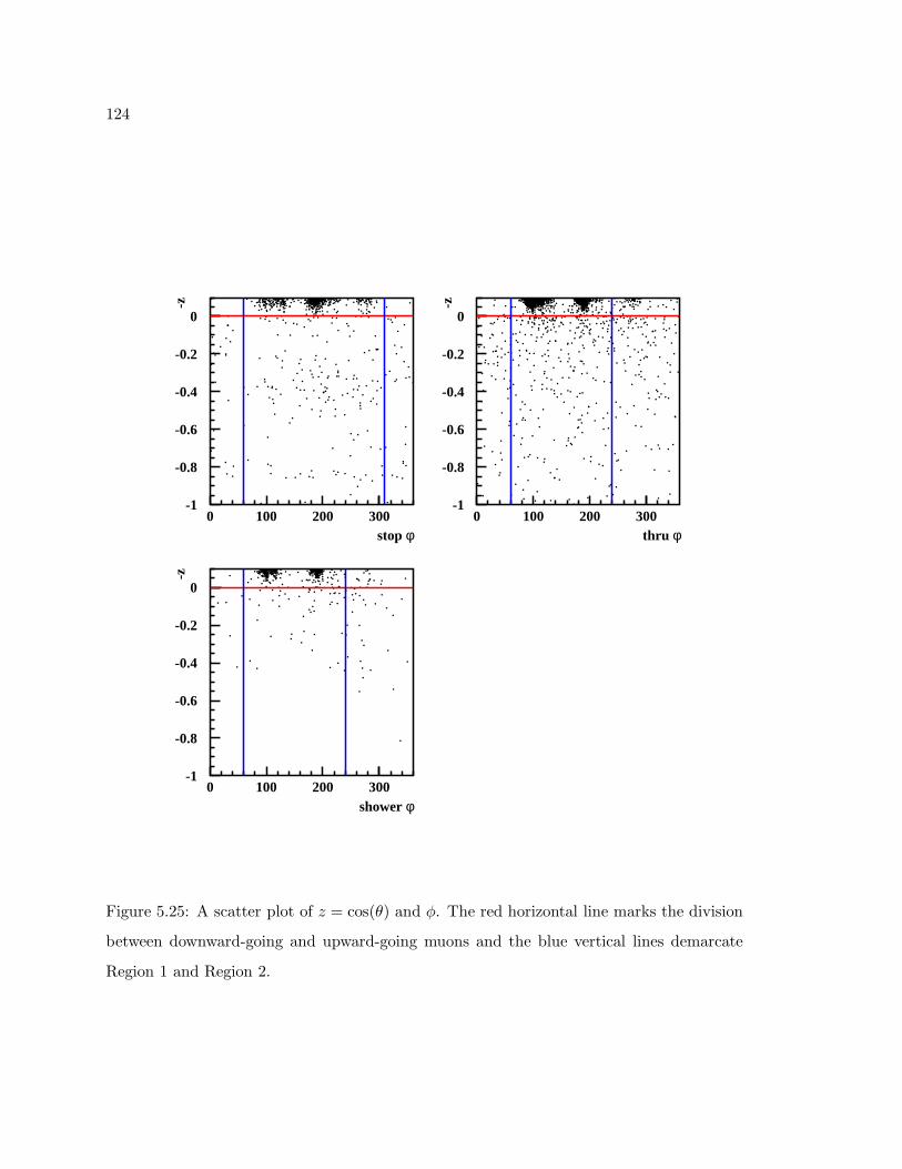
124
-1
-0.8
-0.6
-0.4
-0.2
0
0 100 200 300-1
-0.8
-0.6
-0.4
-0.2
0
0 100 200 300stop φ
-z
thru φ
-z
shower φ
-z
-1
-0.8
-0.6
-0.4
-0.2
0
0 100 200 300
Figure 5.25: A scatter plot of z = cos(θ) and φ. The red horizontal line marks the division
between downward-going and upward-going muons and the blue vertical lines demarcate
Region 1 and Region 2.
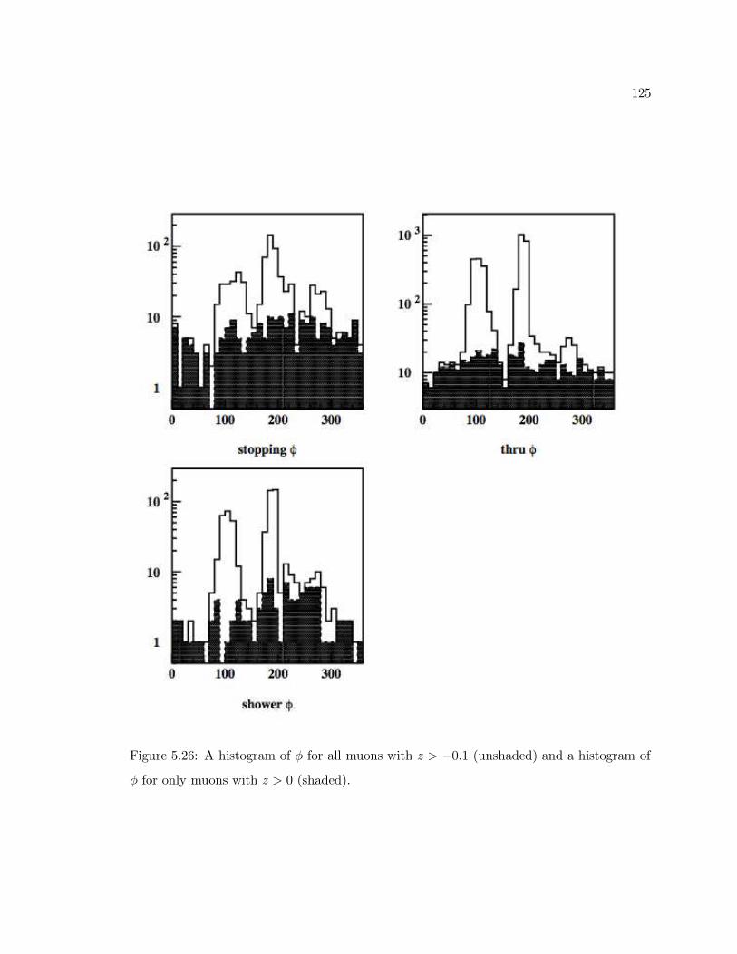
125
Figure 5.26: A histogram of φ for all muons with z > −0.1 (unshaded) and a histogram of
φ for only muons with z > 0 (shaded).
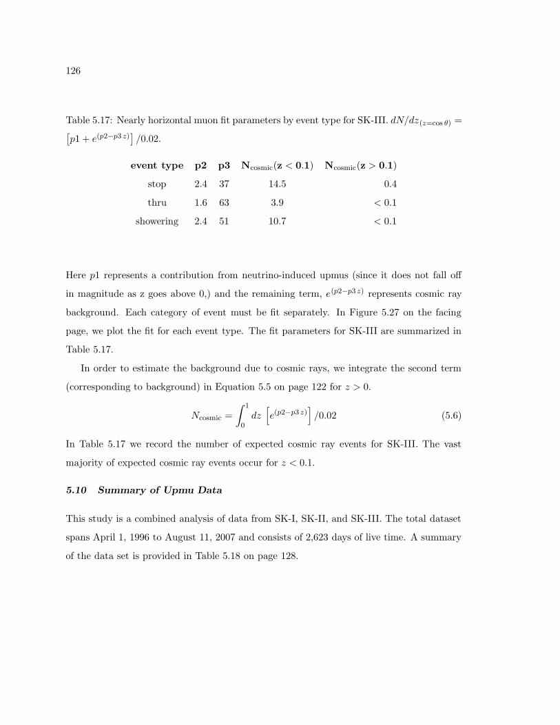
126
Table 5.17: Nearly horizontal muon fit parameters by event type for SK-III. dN/dz(z=cos θ) =[
p1 + e(p2−p3 z)]
/0.02.
event type p2 p3 Ncosmic(z < 0.1) Ncosmic(z > 0.1)
stop 2.4 37 14.5 0.4
thru 1.6 63 3.9 < 0.1
showering 2.4 51 10.7 < 0.1
Here p1 represents a contribution from neutrino-induced upmus (since it does not fall off
in magnitude as z goes above 0,) and the remaining term, e(p2−p3 z) represents cosmic ray
background. Each category of event must be fit separately. In Figure 5.27 on the facing
page, we plot the fit for each event type. The fit parameters for SK-III are summarized in
Table 5.17.
In order to estimate the background due to cosmic rays, we integrate the second term
(corresponding to background) in Equation 5.5 on page 122 for z > 0.
Ncosmic =
∫ 1
0dz[
e(p2−p3 z)]
/0.02 (5.6)
In Table 5.17 we record the number of expected cosmic ray events for SK-III. The vast
majority of expected cosmic ray events occur for z < 0.1.
5.10 Summary of Upmu Data
This study is a combined analysis of data from SK-I, SK-II, and SK-III. The total dataset
spans April 1, 1996 to August 11, 2007 and consists of 2,623 days of live time. A summary
of the data set is provided in Table 5.18 on page 128.
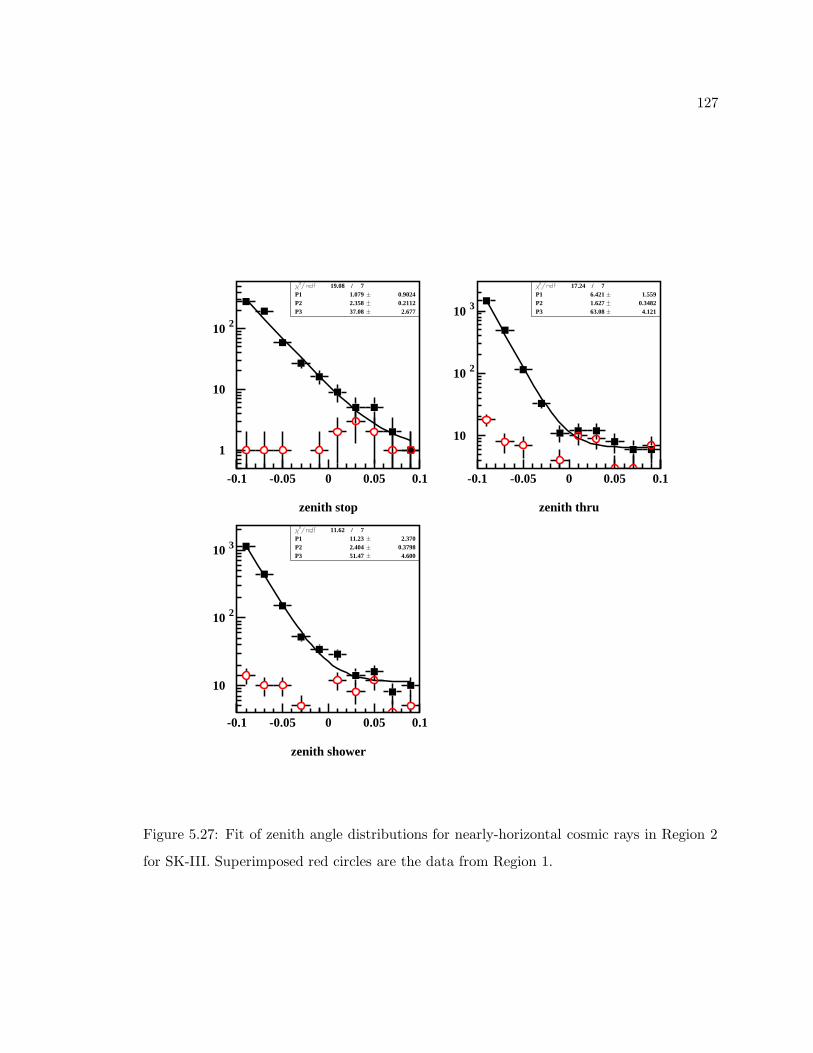
127
zenith stop
1
10
10 2
-0.1 -0.05 0 0.05 0.1
19.08 / 7P1 1.079 0.9024P2 2.358 0.2112P3 37.08 2.677
zenith thru
10
10 2
10 3
-0.1 -0.05 0 0.05 0.1
17.24 / 7P1 6.421 1.559P2 1.627 0.3482P3 63.08 4.121
zenith shower
10
10 2
10 3
-0.1 -0.05 0 0.05 0.1
11.62 / 7P1 11.23 2.370P2 2.404 0.3798P3 51.47 4.600
Figure 5.27: Fit of zenith angle distributions for nearly-horizontal cosmic rays in Region 2
for SK-III. Superimposed red circles are the data from Region 1.
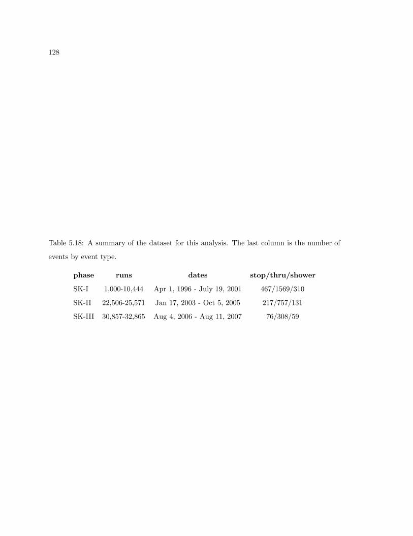
128
Table 5.18: A summary of the dataset for this analysis. The last column is the number of
events by event type.
phase runs dates stop/thru/shower
SK-I 1,000-10,444 Apr 1, 1996 - July 19, 2001 467/1569/310
SK-II 22,506-25,571 Jan 17, 2003 - Oct 5, 2005 217/757/131
SK-III 30,857-32,865 Aug 4, 2006 - Aug 11, 2007 76/308/59
129
Chapter 6
POINT SOURCE SEARCH ALGORITHM
6.1 Design Goals
The algorithm described in this chapter was carefully developed with two design goals in
mind. The first was to develop an analysis method that uses all possible information in
the data to make the strongest possible statement about the flux of neutrino point sources.
Embracing this philosophy, the idealized end product is a “maximally efficient search,” which
represents the limit of what we can hope to know about neutrino point sources using the
Super-Kamiokande detector over the period of operation. The second goal was to develop
the algorithm using only MC to avoid issues with trial factors.
The idea of a maximally efficient search is interesting for a variety of reasons. First,
it is a novel approach to the detection of point source neutrinos with Super-Kamiokande,
and so it is intrinsically interesting from the perspective of data analysis. Second, since
this method has never been used before, it will be additionally interesting to determine
the extent to which such an algorithm can improve over simpler algorithms. The extent
to which the algorithm is interesting to astrophysics, as a tool in the search for neutrino
point sources, will be gauged by the extent to which it improves over previous techniques.
Thus, we aspire to create a maximally efficient algorithm not merely to improve detection
efficiency, but also determine the extent to which that efficiency can be improved.
6.2 Search Algorithm Design
In this section we will outline the design of an algorithm. We will show how we can use
this algorithm to estimate the number of events attributable to signal (point sources) in the
presence of background (due to atmospheric neutrinos and nearly-horizontal cosmic rays.)
Additionally we will show how the algorithm can be used to calculate an upper limit on the
number of signal events and to compute the probability that an apparent signal is due to
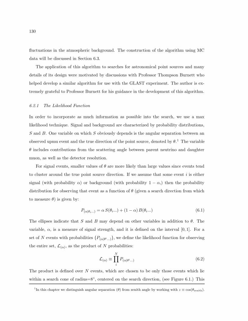
130
fluctuations in the atmospheric background. The construction of the algorithm using MC
data will be discussed in Section 6.3.
The application of this algorithm to searches for astronomical point sources and many
details of its design were motivated by discussions with Professor Thompson Burnett who
helped develop a similar algorithm for use with the GLAST experiment. The author is ex-
tremely grateful to Professor Burnett for his guidance in the development of this algorithm.
6.2.1 The Likelihood Function
In order to incorporate as much information as possible into the search, we use a max
likelihood technique. Signal and background are characterized by probability distributions,
S and B. One variable on which S obviously depends is the angular separation between an
observed upmu event and the true direction of the point source, denoted by θ.1 The variable
θ includes contributions from the scattering angle between parent neutrino and daughter
muon, as well as the detector resolution.
For signal events, smaller values of θ are more likely than large values since events tend
to cluster around the true point source direction. If we assume that some event i is either
signal (with probability α) or background (with probability 1 − α,) then the probability
distribution for observing that event as a function of θ (given a search direction from which
to measure θ) is given by:
P(α|θi...) = αS(θi...) + (1 − α)B(θi...) (6.1)
The ellipses indicate that S and B may depend on other variables in addition to θ. The
variable, α, is a measure of signal strength, and it is defined on the interval [0, 1]. For a
set of N events with probabilities P(α|θi ...), we define the likelihood function for observing
the entire set, L(α), as the product of N probabilities:
L(α) ≡N∏
i
P(α|θi...) (6.2)
The product is defined over N events, which are chosen to be only those events which lie
within a search cone of radius=8, centered on the search direction, (see Figure 6.1.) This
1In this chapter we distinguish angular separation (θ) from zenith angle by working with z ≡ cos(θzenith).
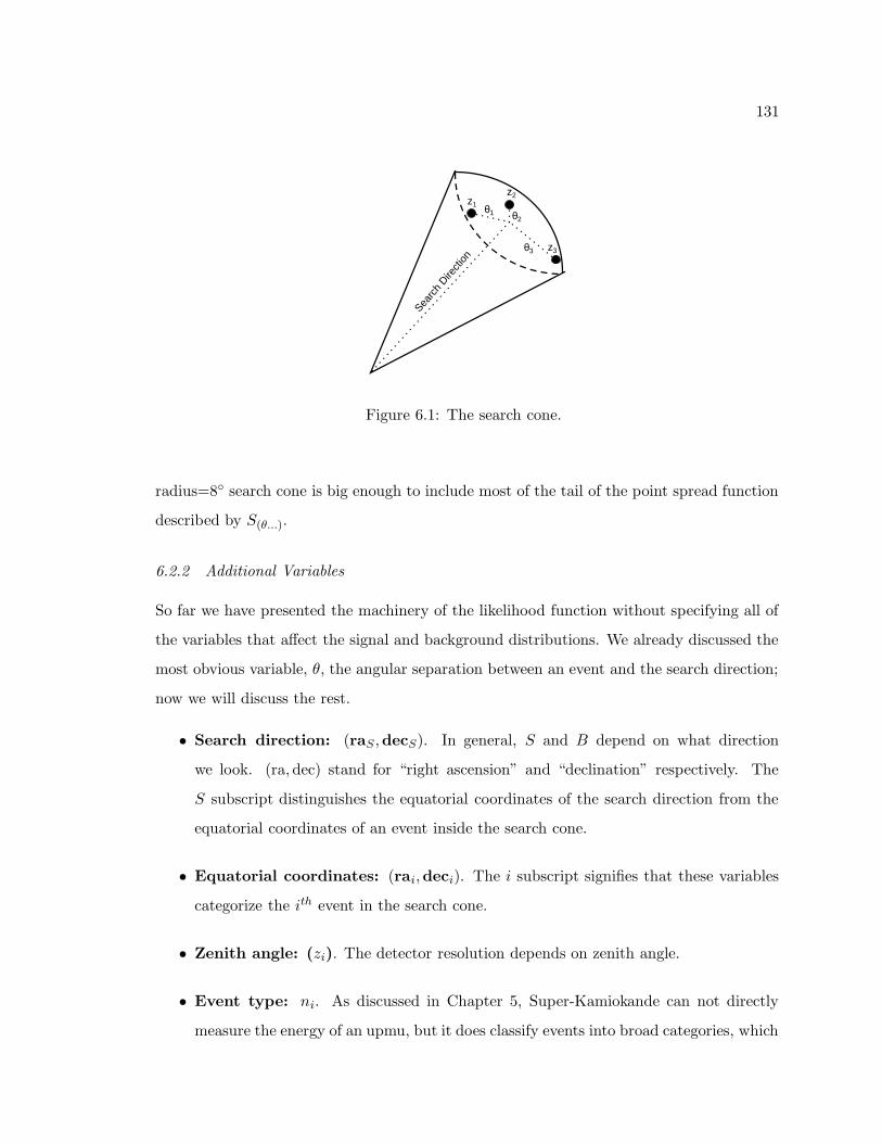
131
z1
z2
z3
θ1 θ2
θ3
Searc
h Dire
ctio
n
Figure 6.1: The search cone.
radius=8 search cone is big enough to include most of the tail of the point spread function
described by S(θ...).
6.2.2 Additional Variables
So far we have presented the machinery of the likelihood function without specifying all of
the variables that affect the signal and background distributions. We already discussed the
most obvious variable, θ, the angular separation between an event and the search direction;
now we will discuss the rest.
• Search direction: (raS ,decS). In general, S and B depend on what direction
we look. (ra,dec) stand for “right ascension” and “declination” respectively. The
S subscript distinguishes the equatorial coordinates of the search direction from the
equatorial coordinates of an event inside the search cone.
• Equatorial coordinates: (rai,deci). The i subscript signifies that these variables
categorize the ith event in the search cone.
• Zenith angle: (zi). The detector resolution depends on zenith angle.
• Event type: ni. As discussed in Chapter 5, Super-Kamiokande can not directly
measure the energy of an upmu, but it does classify events into broad categories, which
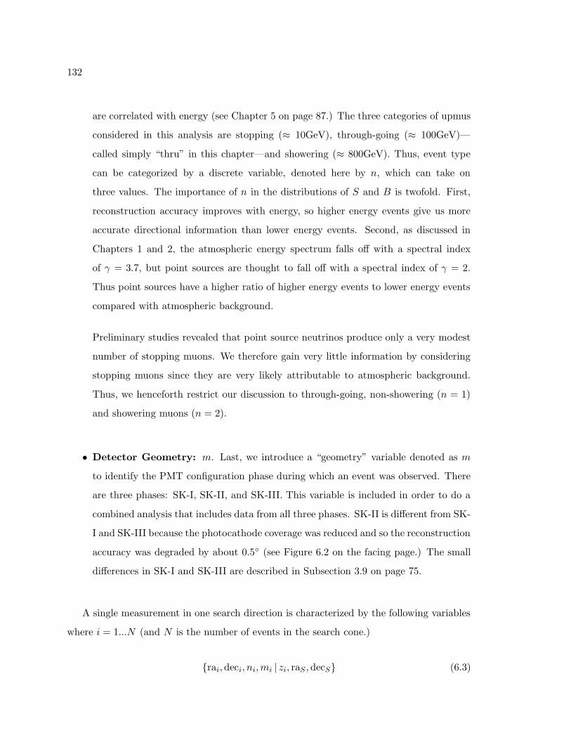
132
are correlated with energy (see Chapter 5 on page 87.) The three categories of upmus
considered in this analysis are stopping (≈ 10GeV), through-going (≈ 100GeV)—
called simply “thru” in this chapter—and showering (≈ 800GeV). Thus, event type
can be categorized by a discrete variable, denoted here by n, which can take on
three values. The importance of n in the distributions of S and B is twofold. First,
reconstruction accuracy improves with energy, so higher energy events give us more
accurate directional information than lower energy events. Second, as discussed in
Chapters 1 and 2, the atmospheric energy spectrum falls off with a spectral index
of γ = 3.7, but point sources are thought to fall off with a spectral index of γ = 2.
Thus point sources have a higher ratio of higher energy events to lower energy events
compared with atmospheric background.
Preliminary studies revealed that point source neutrinos produce only a very modest
number of stopping muons. We therefore gain very little information by considering
stopping muons since they are very likely attributable to atmospheric background.
Thus, we henceforth restrict our discussion to through-going, non-showering (n = 1)
and showering muons (n = 2).
• Detector Geometry: m. Last, we introduce a “geometry” variable denoted as m
to identify the PMT configuration phase during which an event was observed. There
are three phases: SK-I, SK-II, and SK-III. This variable is included in order to do a
combined analysis that includes data from all three phases. SK-II is different from SK-
I and SK-III because the photocathode coverage was reduced and so the reconstruction
accuracy was degraded by about 0.5 (see Figure 6.2 on the facing page.) The small
differences in SK-I and SK-III are described in Subsection 3.9 on page 75.
A single measurement in one search direction is characterized by the following variables
where i = 1...N (and N is the number of events in the search cone.)
rai,deci, ni,mi | zi, raS ,decS (6.3)
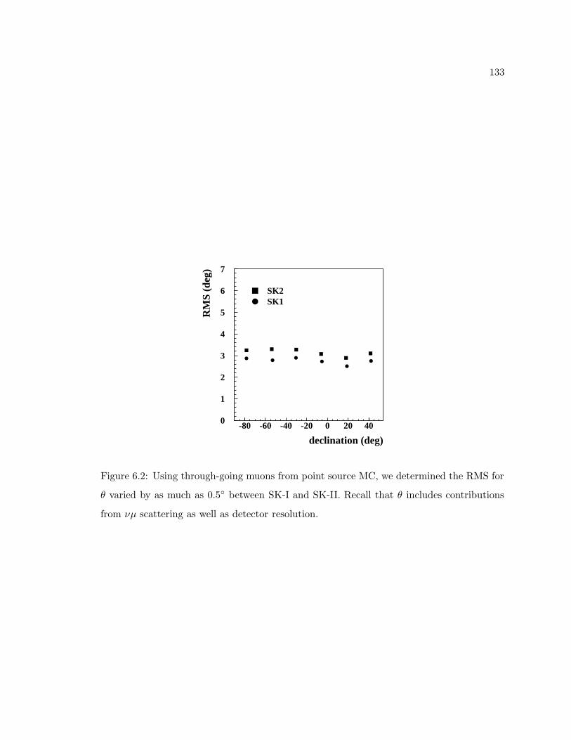
133
SK1SK2
declination (deg)
RM
S (d
eg)
0
1
2
3
4
5
6
7
-80 -60 -40 -20 0 20 40
Figure 6.2: Using through-going muons from point source MC, we determined the RMS for
θ varied by as much as 0.5 between SK-I and SK-II. Recall that θ includes contributions
from νµ scattering as well as detector resolution.
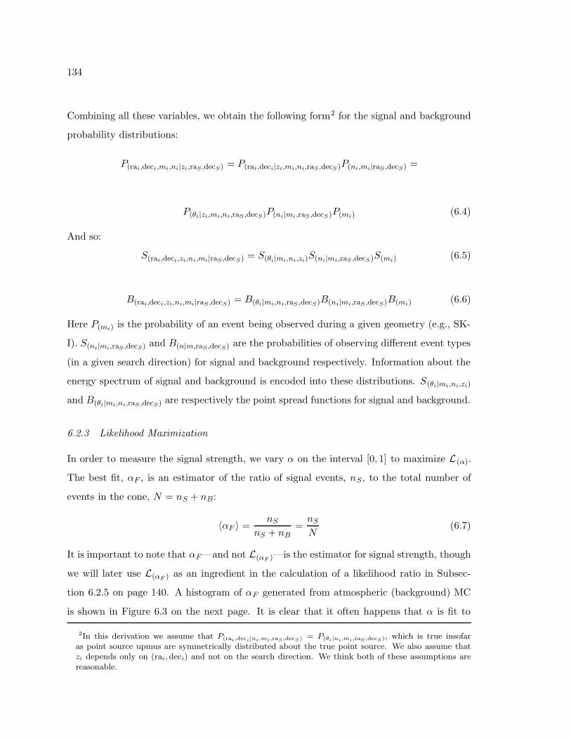
134
Combining all these variables, we obtain the following form2 for the signal and background
probability distributions:
P(rai,deci,mi,ni|zi,raS ,decS) = P(rai,deci|zi,mi,ni,raS ,decS)P(ni,mi|raS ,decS) =
P(θi|zi,mi,ni,raS ,decS)P(ni|mi,raS ,decS)P(mi) (6.4)
And so:
S(rai,deci,zi,ni,mi|raS ,decS) = S(θi|mi,ni,zi)S(ni|mi,raS ,decS)S(mi) (6.5)
B(rai,deci,zi,ni,mi|raS ,decS) = B(θi|mi,ni,raS ,decS)B(ni|mi,raS ,decS)B(mi) (6.6)
Here P(mi) is the probability of an event being observed during a given geometry (e.g., SK-
I). S(ni|mi,raS ,decS) and B(n|m,raS ,decS) are the probabilities of observing different event types
(in a given search direction) for signal and background respectively. Information about the
energy spectrum of signal and background is encoded into these distributions. S(θi|mi,ni,zi)
and B(θi|mi,ni,raS ,decS) are respectively the point spread functions for signal and background.
6.2.3 Likelihood Maximization
In order to measure the signal strength, we vary α on the interval [0, 1] to maximize L(α).
The best fit, αF , is an estimator of the ratio of signal events, nS , to the total number of
events in the cone, N = nS + nB:
〈αF 〉 =nS
nS + nB=nS
N(6.7)
It is important to note that αF—and not L(αF )—is the estimator for signal strength, though
we will later use L(αF ) as an ingredient in the calculation of a likelihood ratio in Subsec-
tion 6.2.5 on page 140. A histogram of αF generated from atmospheric (background) MC
is shown in Figure 6.3 on the next page. It is clear that it often happens that α is fit to
2In this derivation we assume that P(rai,deci|ni,mi,raS ,decS) = P(θi|ni,mi,raS ,decS), which is true insofaras point source upmus are symmetrically distributed about the true point source. We also assume thatzi depends only on (rai, deci) and not on the search direction. We think both of these assumptions arereasonable.
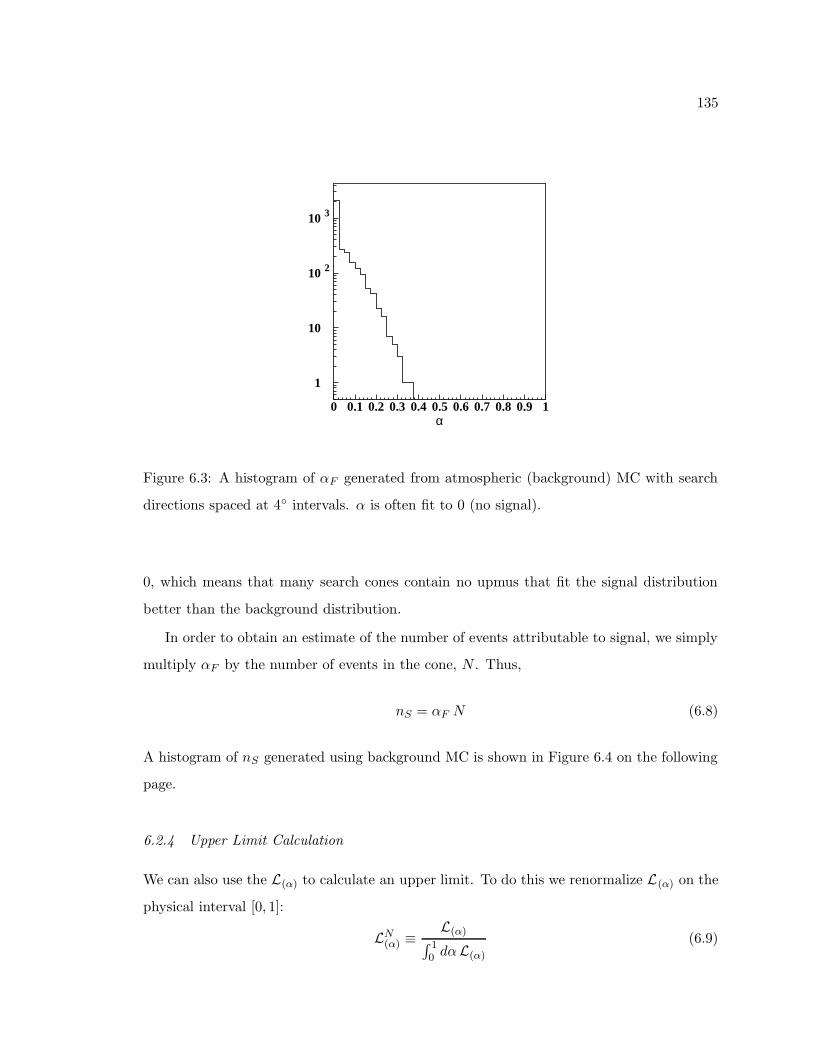
135
α
1
10
10 2
10 3
0 0.1 0.2 0.3 0.4 0.5 0.6 0.7 0.8 0.9 1
Figure 6.3: A histogram of αF generated from atmospheric (background) MC with search
directions spaced at 4 intervals. α is often fit to 0 (no signal).
0, which means that many search cones contain no upmus that fit the signal distribution
better than the background distribution.
In order to obtain an estimate of the number of events attributable to signal, we simply
multiply αF by the number of events in the cone, N . Thus,
nS = αF N (6.8)
A histogram of nS generated using background MC is shown in Figure 6.4 on the following
page.
6.2.4 Upper Limit Calculation
We can also use the L(α) to calculate an upper limit. To do this we renormalize L(α) on the
physical interval [0, 1]:
LN(α) ≡
L(α)∫ 10 dαL(α)
(6.9)
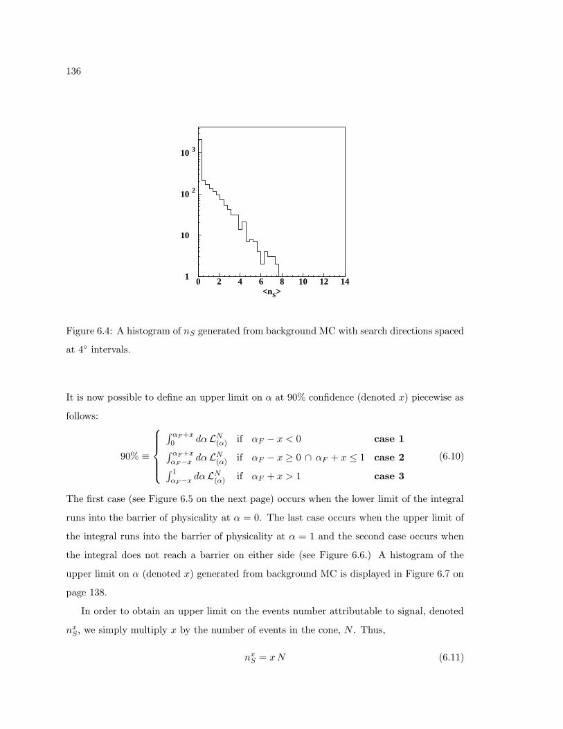
136
<nS>
1
10
10 2
10 3
0 2 4 6 8 10 12 14
Figure 6.4: A histogram of nS generated from background MC with search directions spaced
at 4 intervals.
It is now possible to define an upper limit on α at 90% confidence (denoted x) piecewise as
follows:
90% ≡
∫ αF +x0 dαLN
(α) if αF − x < 0 case 1∫ αF +xαF−x dαLN
(α) if αF − x ≥ 0 ∩ αF + x ≤ 1 case 2∫ 1αF−x dαLN
(α) if αF + x > 1 case 3
(6.10)
The first case (see Figure 6.5 on the next page) occurs when the lower limit of the integral
runs into the barrier of physicality at α = 0. The last case occurs when the upper limit of
the integral runs into the barrier of physicality at α = 1 and the second case occurs when
the integral does not reach a barrier on either side (see Figure 6.6.) A histogram of the
upper limit on α (denoted x) generated from background MC is displayed in Figure 6.7 on
page 138.
In order to obtain an upper limit on the events number attributable to signal, denoted
nxS, we simply multiply x by the number of events in the cone, N . Thus,
nxS = xN (6.11)
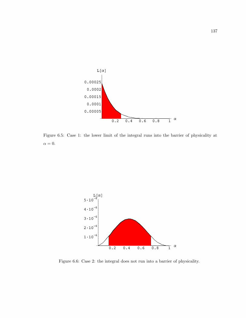
137
0.2 0.4 0.6 0.8 1Α
0.00005
0.0001
0.00015
0.0002
0.00025
L@ΑD
0.2 0.4 0.6 0.8 1Α
0.00005
0.0001
0.00015
0.0002
0.00025
L@ΑD
Figure 6.5: Case 1: the lower limit of the integral runs into the barrier of physicality at
α = 0.
0.2 0.4 0.6 0.8 1Α
1·10-6
2·10-6
3·10-6
4·10-6
5·10-6L@ΑD
0.2 0.4 0.6 0.8 1Α
1·10-6
2·10-6
3·10-6
4·10-6
5·10-6L@ΑD
Figure 6.6: Case 2: the integral does not run into a barrier of physicality.
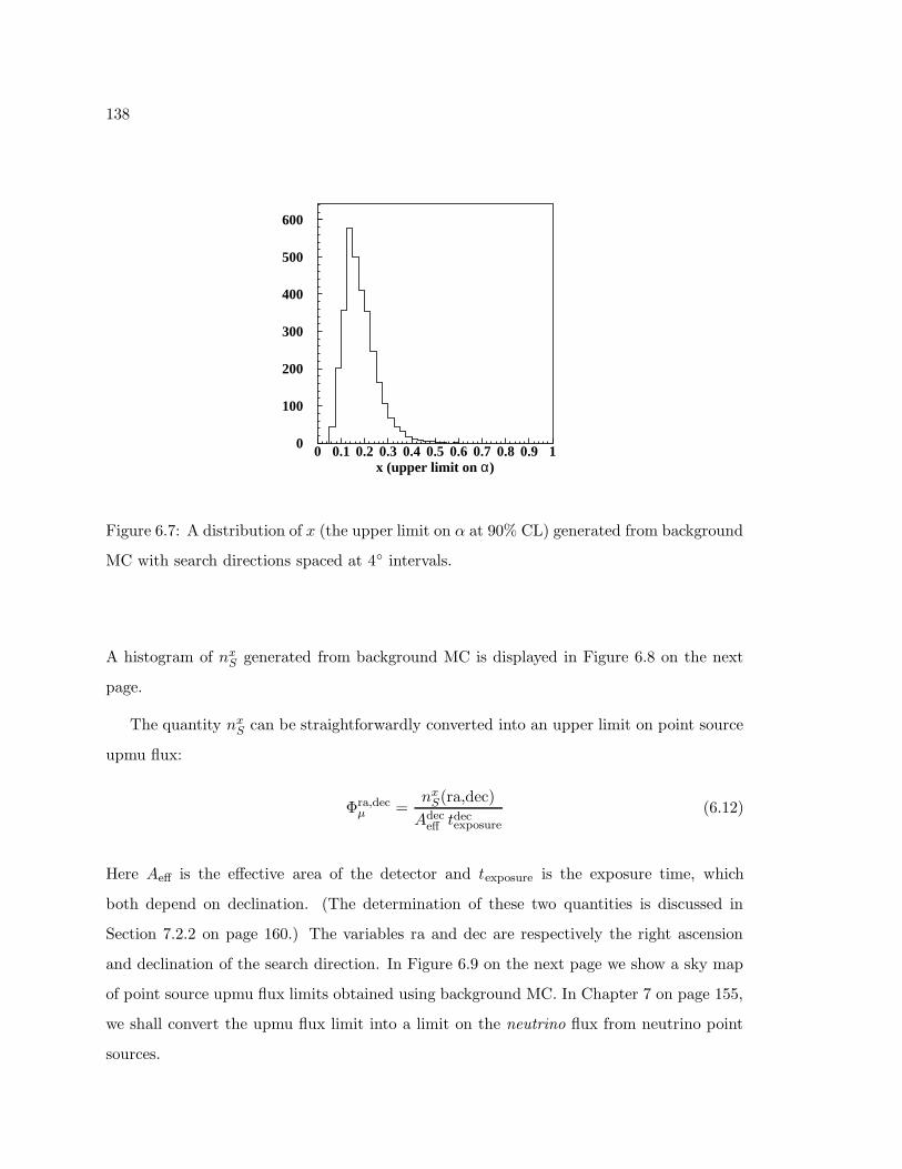
138
x (upper limit on α)
0
100
200
300
400
500
600
0 0.1 0.2 0.3 0.4 0.5 0.6 0.7 0.8 0.9 1
Figure 6.7: A distribution of x (the upper limit on α at 90% CL) generated from background
MC with search directions spaced at 4 intervals.
A histogram of nxS generated from background MC is displayed in Figure 6.8 on the next
page.
The quantity nxS can be straightforwardly converted into an upper limit on point source
upmu flux:
Φra,decµ =
nxS(ra,dec)
Adeceff tdec
exposure
(6.12)
Here Aeff is the effective area of the detector and texposure is the exposure time, which
both depend on declination. (The determination of these two quantities is discussed in
Section 7.2.2 on page 160.) The variables ra and dec are respectively the right ascension
and declination of the search direction. In Figure 6.9 on the next page we show a sky map
of point source upmu flux limits obtained using background MC. In Chapter 7 on page 155,
we shall convert the upmu flux limit into a limit on the neutrino flux from neutrino point
sources.
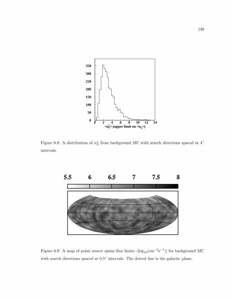
139
<nxS> (upper limit on <nS>)
0
50
100
150
200
250
300
350
0 2 4 6 8 10 12 14
Figure 6.8: A distribution of nxS from background MC with search directions spaced at 4
intervals.
Figure 6.9: A map of point source upmu flux limits -[log10(cm−2s−1)] for background MC
with search directions spaced at 0.5 intervals. The dotted line is the galactic plane.
140
6.2.5 Computing Significance with the Likelihood Ratio
So far we have discussed how to use L(α) to determine signal strength (αF ) and to calculate
an upper limit on signal strength (x). Statements about signal strength are, in turn, con-
verted into statements about flux. We can also use L(α) to calculate the probability that an
apparent signal is due to fluctuations in the atmospheric background. In order to do this
we define a likelihood ratio (denoted Λ):
Λ ≡ 2 log[L(αF )/L(α = 0)] (6.13)
As αF increases, Λ increases, and the the probability of observing that value of Λ decreases
according approximately to a χ2 distribution with one degree of freedom. About half of the
time Λ is fit to Λ = 0 because none of the events in the search cone are likely to be signal.
Looking at the Λ distribution, we observe a great number of events in the the smallest bin
(from Λ = 0) so that it no longer resembles a χ2 distribution. Figure 6.10 on the next page
is a histogram of Λ generated using a single background MC sky map.
By generating many background MC sky maps, we can make a histogram of the max-
imum Λ for each map (see Figure 6.11 on page 142,) and use this histogram to assess the
probability of observing a large fluctuation on a single map. This method is convenient be-
cause the histogram in Figure 6.11 that we use to calculate confidence limits automatically
takes into account the number of search directions.
Using this method, we find that the threshold for detection at 90%/99% CL is Λ90%/Λ99% =
30.2/34.7 (for sky maps with search directions spaced at 0.5 intervals.) Signals of approx-
imately 10/11 upmus out of 3,134 total events (≈ 0.3%) are required in order to produce
such large values of Λmax 50% of the time. Signals of approximately 13/15 upmus out of
3,134 total events are required in order to produce such large values of Λmax 90% of the time,
(see Figure 6.12.) (Here we are making a distinction between the false alarm rate, which
determines the threshold for Λ90%/Λ99%, and the detection rate, which tells us the proba-
bility that a true signal will exceed the thresholds.) Thus it is possible to claim a detection
with a signal of about 10 events out of the expected data set of 3,134. Assuming the source
has a spectral index of γ = 2, this corresponds to a neutrino flux of ≈ 3 × 10⁻⁷ cm−2s−1.
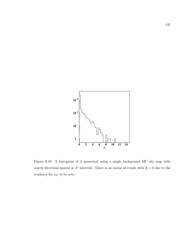
141
Λ
1
10
10 2
10 3
0 2 4 6 8 10 12 14
Figure 6.10: A histogram of Λ generated using a single background MC sky map with
search directions spaced at 4 intervals. There is an excess of events with Λ = 0 due to the
tendency for αF to be zero.
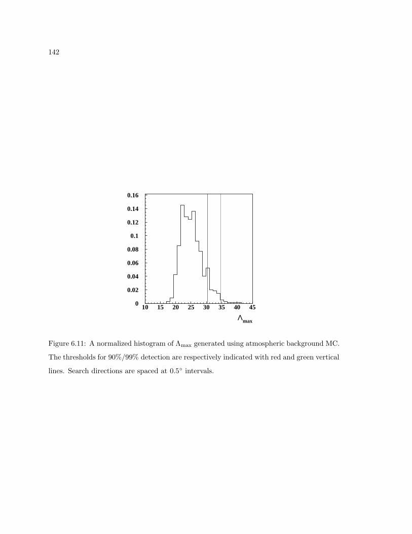
142
Λmax
0
0.02
0.04
0.06
0.08
0.1
0.12
0.14
0.16
10 15 20 25 30 35 40 45
Figure 6.11: A normalized histogram of Λmax generated using atmospheric background MC.
The thresholds for 90%/99% detection are respectively indicated with red and green vertical
lines. Search directions are spaced at 0.5 intervals.
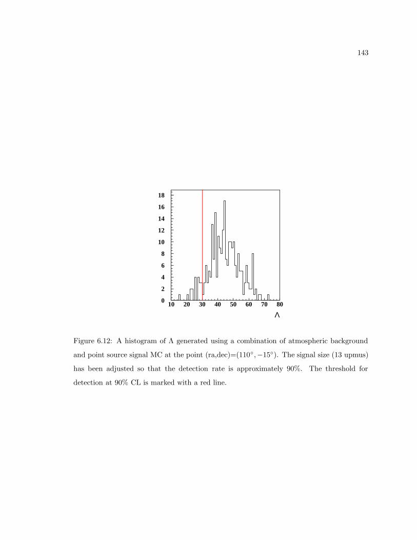
143
Λ
0
2
4
6
8
10
12
14
16
18
10 20 30 40 50 60 70 80
Figure 6.12: A histogram of Λ generated using a combination of atmospheric background
and point source signal MC at the point (ra,dec)=(110,−15). The signal size (13 upmus)
has been adjusted so that the detection rate is approximately 90%. The threshold for
detection at 90% CL is marked with a red line.
144
6.2.6 Performance
The stated goal of this chapter is to develop a maximally efficient search algorithm, and so
in this Subsection we compare its performance with a previous Super-Kamiokande result. In
Reference [14], a simpler cone search was used to test the SK-I data for point sources. A 4
half-angle cone was employed to search the showering muon sample; non-showering muons
were excluded in order to achieve a higher energy sample. A signal was identified as an excess
of events in the search cone. Thus, the test is similar to this one except it does not include
information about non-showering muons and replaces the point spread function S(θ) with
a binary cone test: all events inside the cone are treated equally regardless of their angular
separation from the search direction. An additional difference is that search directions were
chosen to be in the direction of each event, (which was subsequently excluded from the
search cone surrounding it.) We henceforth refer to the algorithm from Reference [14] as
“the hard cone algorithm.”
For a quick and approximate calculation, we consider the coordinates (dec,ra)=(−15, 90)
and take the results to be typical. Employing the hard cone algorithm to the combined SK-I
through SK-III data set, we find an expected background of 0.9 showering events. If we
carry out this test for each showering muon in the data set (≈ 700 times,) we would require
one incident of 7 showering events in order to claim detection at 90% CL. An additional
showering muon is needed to define the search direction, bringing the required signal to 8
showering muons. If there are 8 showering events in a 4 cone, however, there are on average
19 events (including non-showering) in an 8 cone. This is because a 4 cone includes only
≈ 88% of the point spread function, and also because showering muons make up only about
half of the signal from a point source.3 Thus, we find that the algorithm presented here can
improve on the simpler hard cone algorithm by approximately a factor of two.
Detection potential aside, the hard cone algorithm will have a tendency to underestimate
the upper limits on neutrino flux unless it is taken into account that that no more than
3It may be objected that the hard cone test can be extended to 8—like the algorithm presented here—toinclude the vast majority of the point spread function. This would probably worsen its performance,however, since the expanded cone would let in much more background without gaining much signal. Thealgorithm presented here, however, can utilize an arbitrarily big cone since it uses angular separation todistinguish signal from background.
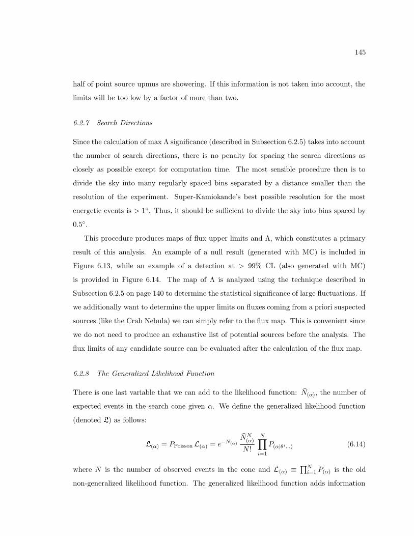
145
half of point source upmus are showering. If this information is not taken into account, the
limits will be too low by a factor of more than two.
6.2.7 Search Directions
Since the calculation of max Λ significance (described in Subsection 6.2.5) takes into account
the number of search directions, there is no penalty for spacing the search directions as
closely as possible except for computation time. The most sensible procedure then is to
divide the sky into many regularly spaced bins separated by a distance smaller than the
resolution of the experiment. Super-Kamiokande’s best possible resolution for the most
energetic events is > 1. Thus, it should be sufficient to divide the sky into bins spaced by
0.5.
This procedure produces maps of flux upper limits and Λ, which constitutes a primary
result of this analysis. An example of a null result (generated with MC) is included in
Figure 6.13, while an example of a detection at > 99% CL (also generated with MC)
is provided in Figure 6.14. The map of Λ is analyzed using the technique described in
Subsection 6.2.5 on page 140 to determine the statistical significance of large fluctuations. If
we additionally want to determine the upper limits on fluxes coming from a priori suspected
sources (like the Crab Nebula) we can simply refer to the flux map. This is convenient since
we do not need to produce an exhaustive list of potential sources before the analysis. The
flux limits of any candidate source can be evaluated after the calculation of the flux map.
6.2.8 The Generalized Likelihood Function
There is one last variable that we can add to the likelihood function: N(α), the number of
expected events in the search cone given α. We define the generalized likelihood function
(denoted ) as follows:
(α) = PPoisson L(α) = e−N(α)NN
(α)
N !
N∏
i=1
P(α|θi...) (6.14)
where N is the number of observed events in the cone and L(α) ≡ ∏Ni=1 P(α) is the old
non-generalized likelihood function. The generalized likelihood function adds information
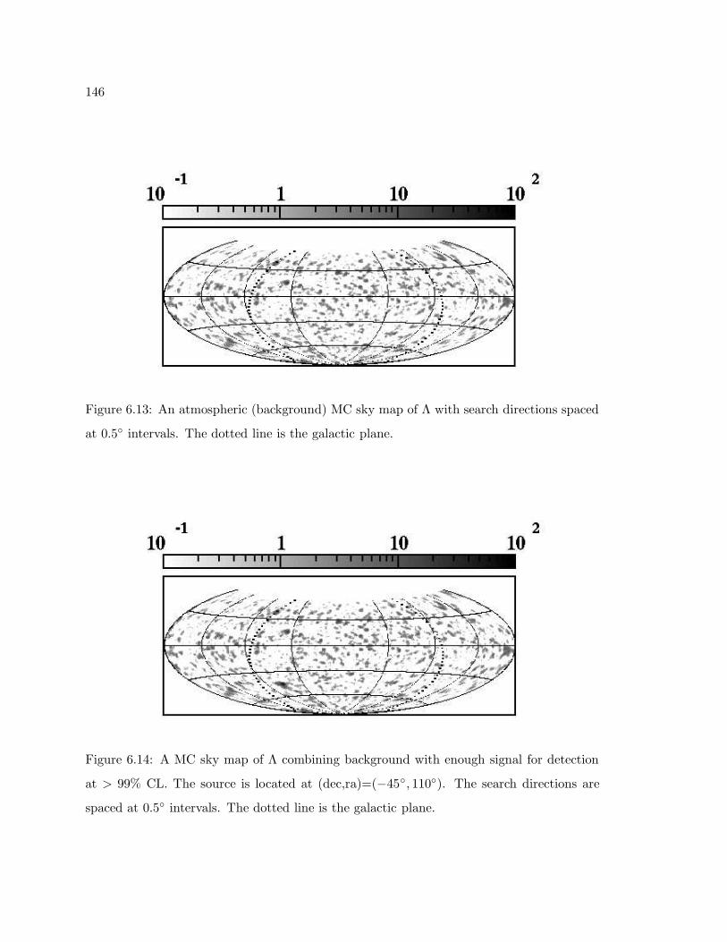
146
Figure 6.13: An atmospheric (background) MC sky map of Λ with search directions spaced
at 0.5 intervals. The dotted line is the galactic plane.
Figure 6.14: A MC sky map of Λ combining background with enough signal for detection
at > 99% CL. The source is located at (dec,ra)=(−45, 110). The search directions are
spaced at 0.5 intervals. The dotted line is the galactic plane.
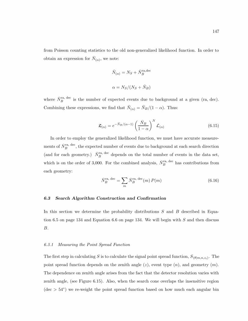
147
from Poisson counting statistics to the old non-generalized likelihood function. In order to
obtain an expression for N(α), we note:
N(α) = NS + N ra,decB
α = NS/(NS + NB)
where N ra, decB is the number of expected events due to background at a given (ra, dec).
Combining these expressions, we find that N(α) = NB/(1 − α). Thus:
(α) = e−NB/(α−1)
(
NB
1 − α
)N
L(α) (6.15)
In order to employ the generalized likelihood function, we must have accurate measure-
ments of N ra, decB , the expected number of events due to background at each search direction
(and for each geometry.) N ra, decB depends on the total number of events in the data set,
which is on the order of 3,000. For the combined analysis, N ra, decB has contributions from
each geometry:
N ra, decB =
∑
m
N ra, decB (m)P (m) (6.16)
6.3 Search Algorithm Construction and Confirmation
In this section we determine the probability distributions S and B described in Equa-
tion 6.5 on page 134 and Equation 6.6 on page 134. We will begin with S and then discuss
B.
6.3.1 Measuring the Point Spread Function
The first step in calculating S is to calculate the signal point spread function, S(θ|m,n,zi). The
point spread function depends on the zenith angle (z), event type (n), and geometry (m).
The dependence on zenith angle arises from the fact that the detector resolution varies with
zenith angle, (see Figure 6.15). Also, when the search cone overlaps the insensitive region
(dec > 54) we re-weight the point spread function based on how much each angular bin
148
0
0.1
0.2
0.3
0.4
0.5
0 1 2 3 4 5 6 7 8
z<0.25
z>0.75
θ (deg)
Figure 6.15: The point spread function at two different different regions of zenith angle.
overlaps the insensitive region.4 The value of geometry (m) is set when running skdetsim
by selecting the appropriate skx odtune.card file. The upmu reduction has separate code
for SK-I, SK-II and SK-III. The output of the upmu reduction is a .zbs file, which is then
given to fillnt in order to create an ntuple.
We compare the parent neutrino direction with the fitted muon direction and determine
the angular separation, θ. At this stage we can also select events based on their type (n =
thru or shower). In this way we generate a histogram of θ for a given combination of m, n
and z as in Figure 6.16 on the facing page.
Thrumus have an average angular separation of 1.3, (due to scattering as well as detector
resolution,) while showering muons have average angular separations of 1.2. (These angular
separations are small compared to the resolutions quoted in Section 5.5.1 on page 97, which
were determined using atmospheric MC, because point source MC is peaked at a higher
energy.) There are three competing effects which affect how resolution varies with energy.
4 The kth bin is re-weighted by [π + q 1 − q2 − cos−1 (q)]/π where q ≡ (54− dec)/θk and θk is the
maximum angle of the kth bin.
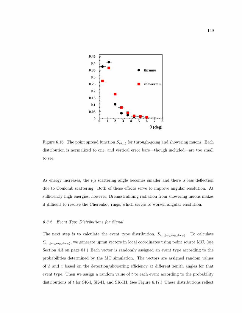
149
thrumu
showermu
θ (deg)
0
0.05
0.1
0.15
0.2
0.25
0.3
0.35
0.4
0.45
0 1 2 3 4 5 6 7 8
Figure 6.16: The point spread function S(θ...) for through-going and showering muons. Each
distribution is normalized to one, and vertical error bars—though included—are too small
to see.
As energy increases, the νµ scattering angle becomes smaller and there is less deflection
due to Coulomb scattering. Both of these effects serve to improve angular resolution. At
sufficiently high energies, however, Bremsstrahlung radiation from showering muons makes
it difficult to resolve the Cherenkov rings, which serves to worsen angular resolution.
6.3.2 Event Type Distributions for Signal
The next step is to calculate the event type distribution, S(ni|mi,raS ,decS). To calculate
S(ni|mi,raS ,decS), we generate upmu vectors in local coordinates using point source MC, (see
Section 4.3 on page 81.) Each vector is randomly assigned an event type according to the
probabilities determined by the MC simulation. The vectors are assigned random values
of φ and z based on the detection/showering efficiency at different zenith angles for that
event type. Then we assign a random value of t to each event according to the probability
distributions of t for SK-I, SK-II, and SK-III, (see Figure 6.17.) These distributions reflect
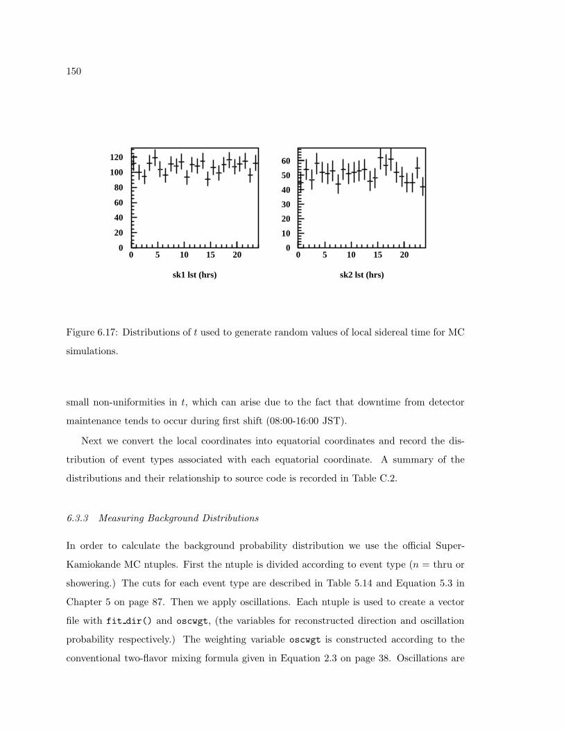
150
sk1 lst (hrs) sk2 lst (hrs)
0
20
40
60
80
100
120
0 5 10 15 200
10
20
30
40
50
60
0 5 10 15 20
Figure 6.17: Distributions of t used to generate random values of local sidereal time for MC
simulations.
small non-uniformities in t, which can arise due to the fact that downtime from detector
maintenance tends to occur during first shift (08:00-16:00 JST).
Next we convert the local coordinates into equatorial coordinates and record the dis-
tribution of event types associated with each equatorial coordinate. A summary of the
distributions and their relationship to source code is recorded in Table C.2.
6.3.3 Measuring Background Distributions
In order to calculate the background probability distribution we use the official Super-
Kamiokande MC ntuples. First the ntuple is divided according to event type (n = thru or
showering.) The cuts for each event type are described in Table 5.14 and Equation 5.3 in
Chapter 5 on page 87. Then we apply oscillations. Each ntuple is used to create a vector
file with fit dir() and oscwgt, (the variables for reconstructed direction and oscillation
probability respectively.) The weighting variable oscwgt is constructed according to the
conventional two-flavor mixing formula given in Equation 2.3 on page 38. Oscillations are
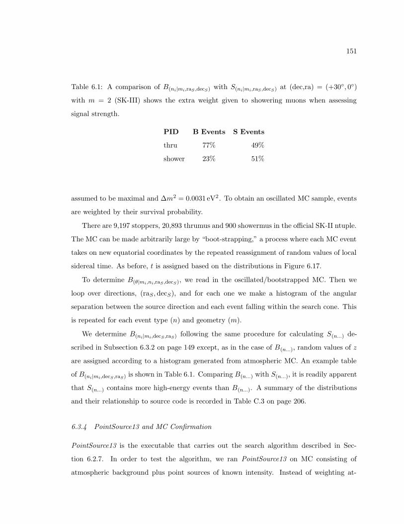
151
Table 6.1: A comparison of B(ni|mi,raS ,decS) with S(ni|mi,raS ,decS) at (dec,ra) = (+30, 0)
with m = 2 (SK-III) shows the extra weight given to showering muons when assessing
signal strength.
PID B Events S Events
thru 77% 49%
shower 23% 51%
assumed to be maximal and ∆m2 = 0.0031 eV2 . To obtain an oscillated MC sample, events
are weighted by their survival probability.
There are 9,197 stoppers, 20,893 thrumus and 900 showermus in the official SK-II ntuple.
The MC can be made arbitrarily large by “boot-strapping,” a process where each MC event
takes on new equatorial coordinates by the repeated reassignment of random values of local
sidereal time. As before, t is assigned based on the distributions in Figure 6.17.
To determine B(θ|mi,ni,raS ,decS), we read in the oscillated/bootstrapped MC. Then we
loop over directions, (raS ,decS), and for each one we make a histogram of the angular
separation between the source direction and each event falling within the search cone. This
is repeated for each event type (n) and geometry (m).
We determine B(ni|mi,decS ,raS) following the same procedure for calculating S(n...) de-
scribed in Subsection 6.3.2 on page 149 except, as in the case of B(n...), random values of z
are assigned according to a histogram generated from atmospheric MC. An example table
of B(ni|mi,decS ,raS) is shown in Table 6.1. Comparing B(n...) with S(n...), it is readily apparent
that S(n...) contains more high-energy events than B(n...). A summary of the distributions
and their relationship to source code is recorded in Table C.3 on page 206.
6.3.4 PointSource13 and MC Confirmation
PointSource13 is the executable that carries out the search algorithm described in Sec-
tion 6.2.7. In order to test the algorithm, we ran PointSource13 on MC consisting of
atmospheric background plus point sources of known intensity. Instead of weighting at-
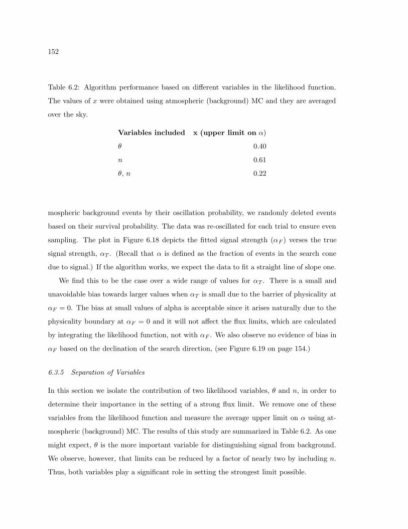
152
Table 6.2: Algorithm performance based on different variables in the likelihood function.
The values of x were obtained using atmospheric (background) MC and they are averaged
over the sky.
Variables included x (upper limit on α)
θ 0.40
n 0.61
θ, n 0.22
mospheric background events by their oscillation probability, we randomly deleted events
based on their survival probability. The data was re-oscillated for each trial to ensure even
sampling. The plot in Figure 6.18 depicts the fitted signal strength (αF ) verses the true
signal strength, αT . (Recall that α is defined as the fraction of events in the search cone
due to signal.) If the algorithm works, we expect the data to fit a straight line of slope one.
We find this to be the case over a wide range of values for αT . There is a small and
unavoidable bias towards larger values when αT is small due to the barrier of physicality at
αF = 0. The bias at small values of alpha is acceptable since it arises naturally due to the
physicality boundary at αF = 0 and it will not affect the flux limits, which are calculated
by integrating the likelihood function, not with αF . We also observe no evidence of bias in
αF based on the declination of the search direction, (see Figure 6.19 on page 154.)
6.3.5 Separation of Variables
In this section we isolate the contribution of two likelihood variables, θ and n, in order to
determine their importance in the setting of a strong flux limit. We remove one of these
variables from the likelihood function and measure the average upper limit on α using at-
mospheric (background) MC. The results of this study are summarized in Table 6.2. As one
might expect, θ is the more important variable for distinguishing signal from background.
We observe, however, that limits can be reduced by a factor of nearly two by including n.
Thus, both variables play a significant role in setting the strongest limit possible.
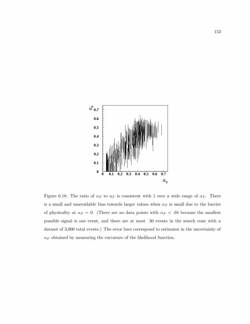
153
αT
α F
0
0.1
0.2
0.3
0.4
0.5
0.6
0.7
0 0.1 0.2 0.3 0.4 0.5 0.6 0.7
Figure 6.18: The ratio of αF to αT is consistent with 1 over a wide range of αT . There
is a small and unavoidable bias towards larger values when αT is small due to the barrier
of physicality at αF = 0. (There are no data points with αF < .04 because the smallest
possible signal is one event, and there are at most 30 events in the search cone with a
dataset of 3,000 total events.) The error bars correspond to estimates in the uncertainty of
αF obtained by measuring the curvature of the likelihood function.
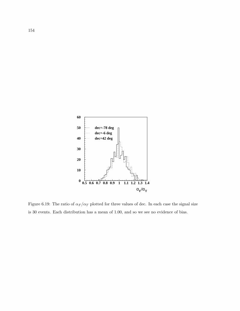
154
dec=-78 degdec=-6 degdec=42 deg
αF/αT
0
10
20
30
40
50
60
0.5 0.6 0.7 0.8 0.9 1 1.1 1.2 1.3 1.4
Figure 6.19: The ratio of αF /αT plotted for three values of dec. In each case the signal size
is 30 events. Each distribution has a mean of 1.00, and so we see no evidence of bias.
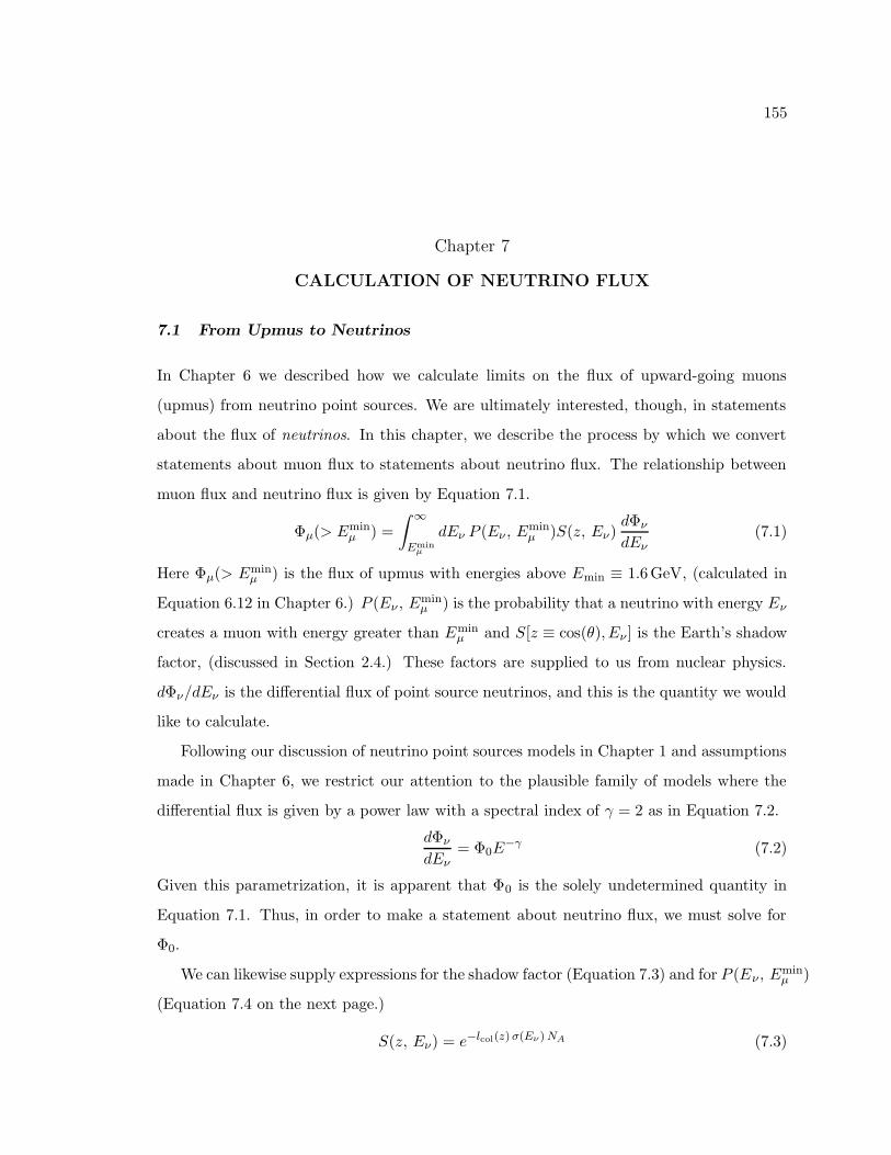
155
Chapter 7
CALCULATION OF NEUTRINO FLUX
7.1 From Upmus to Neutrinos
In Chapter 6 we described how we calculate limits on the flux of upward-going muons
(upmus) from neutrino point sources. We are ultimately interested, though, in statements
about the flux of neutrinos. In this chapter, we describe the process by which we convert
statements about muon flux to statements about neutrino flux. The relationship between
muon flux and neutrino flux is given by Equation 7.1.
Φµ(> Eminµ ) =
∫ ∞
Eminµ
dEν P (Eν , Eminµ )S(z, Eν)
dΦν
dEν(7.1)
Here Φµ(> Eminµ ) is the flux of upmus with energies above Emin ≡ 1.6GeV, (calculated in
Equation 6.12 in Chapter 6.) P (Eν , Eminµ ) is the probability that a neutrino with energy Eν
creates a muon with energy greater than Eminµ and S[z ≡ cos(θ), Eν ] is the Earth’s shadow
factor, (discussed in Section 2.4.) These factors are supplied to us from nuclear physics.
dΦν/dEν is the differential flux of point source neutrinos, and this is the quantity we would
like to calculate.
Following our discussion of neutrino point sources models in Chapter 1 and assumptions
made in Chapter 6, we restrict our attention to the plausible family of models where the
differential flux is given by a power law with a spectral index of γ = 2 as in Equation 7.2.
dΦν
dEν= Φ0E
−γ (7.2)
Given this parametrization, it is apparent that Φ0 is the solely undetermined quantity in
Equation 7.1. Thus, in order to make a statement about neutrino flux, we must solve for
Φ0.
We can likewise supply expressions for the shadow factor (Equation 7.3) and for P (Eν , Eminµ )
(Equation 7.4 on the next page.)
S(z, Eν) = e−lcol(z) σ(Eν) NA (7.3)
156
θ (rad)
colu
mn
dens
ity
(cm
we)
10 8
10 9
10 10
-0.2 0 0.2 0.4 0.6 0.8 1 1.2 1.4 1.6
Figure 7.1: The column depth of the Earth as a function of zenith angle. The data is from
Reference [9].
Here lcol(z) is the Earth’s (zenith angle-dependent) column depth measured in centimeters
water equivalent (or “cmwe,”) σ(Eν) ≡ σCC + σNC is neutrino-nucleon cross section1, and
NA is Avogadro’s number scaled by the density of water (to offset the cmwe unit in the
column depth): NA = 6.022 × 1023 cm−3. The column depth, calculated in Reference [9]
using the “Preliminary Earth Model,” is plotted in Figure 7.1.
P (Eν , Eminµ ) = NA
∫ Eν
0dEµ
dσCC
dEµ(Eµ, Eν)R(Eµ, E
minµ ) (7.4)
Here dσCC/dEµ(Eµ, Eν) is the charged current component of the neutrino-nucleon cross sec-
tion from Reference [119]; (neutral current interactions do not produce muons.) R(Eµ, Eminµ ),
meanwhile, is the average range for a muon with an initial energy of Eµ and a final energy
of Eν from Reference [121].
Armed with numerical representations of P (Eν , Eminµ ) and S(z, Eν), we are ready to
1Though neutral current interactions do not produce upmus, they do contribute to the attenuation ofneutrinos due to the Earth shadow.
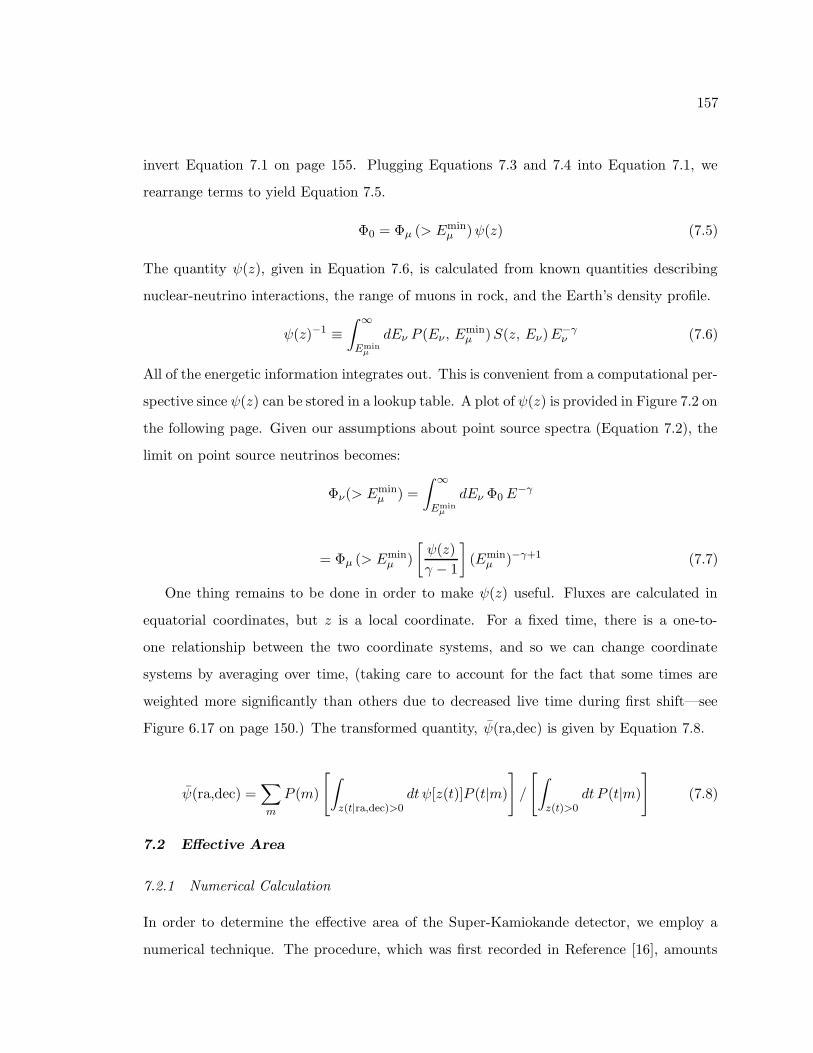
157
invert Equation 7.1 on page 155. Plugging Equations 7.3 and 7.4 into Equation 7.1, we
rearrange terms to yield Equation 7.5.
Φ0 = Φµ (> Eminµ )ψ(z) (7.5)
The quantity ψ(z), given in Equation 7.6, is calculated from known quantities describing
nuclear-neutrino interactions, the range of muons in rock, and the Earth’s density profile.
ψ(z)−1 ≡∫ ∞
Eminµ
dEν P (Eν , Eminµ )S(z, Eν)E
−γν (7.6)
All of the energetic information integrates out. This is convenient from a computational per-
spective since ψ(z) can be stored in a lookup table. A plot of ψ(z) is provided in Figure 7.2 on
the following page. Given our assumptions about point source spectra (Equation 7.2), the
limit on point source neutrinos becomes:
Φν(> Eminµ ) =
∫ ∞
Eminµ
dEν Φ0E−γ
= Φµ (> Eminµ )
[
ψ(z)
γ − 1
]
(Eminµ )−γ+1 (7.7)
One thing remains to be done in order to make ψ(z) useful. Fluxes are calculated in
equatorial coordinates, but z is a local coordinate. For a fixed time, there is a one-to-
one relationship between the two coordinate systems, and so we can change coordinate
systems by averaging over time, (taking care to account for the fact that some times are
weighted more significantly than others due to decreased live time during first shift—see
Figure 6.17 on page 150.) The transformed quantity, ψ(ra,dec) is given by Equation 7.8.
ψ(ra,dec) =∑
m
P (m)
[
∫
z(t|ra,dec)>0dt ψ[z(t)]P (t|m)
]
/
[
∫
z(t)>0dt P (t|m)
]
(7.8)
7.2 Effective Area
7.2.1 Numerical Calculation
In order to determine the effective area of the Super-Kamiokande detector, we employ a
numerical technique. The procedure, which was first recorded in Reference [16], amounts
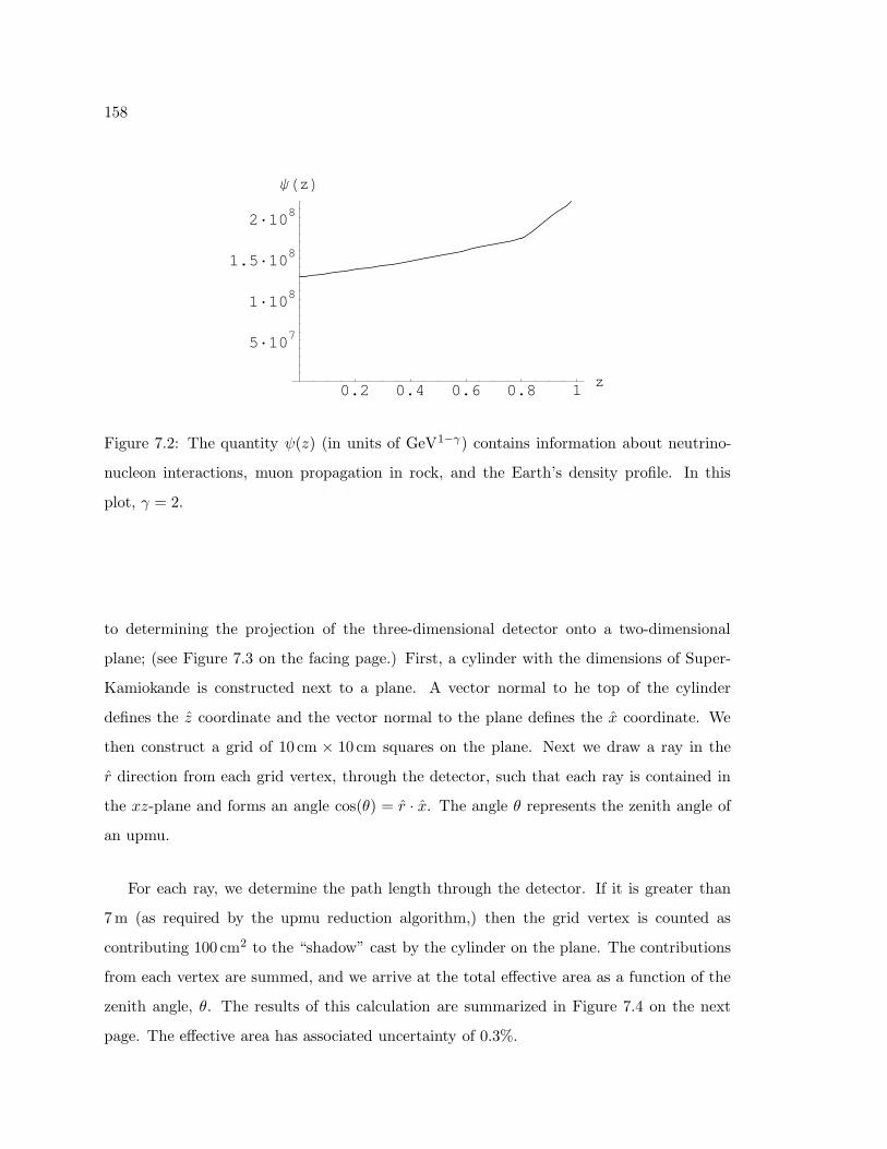
158
0.2 0.4 0.6 0.8 1z
5·107
1·108
1.5·108
2·108
ΨHzL
Figure 7.2: The quantity ψ(z) (in units of GeV1−γ) contains information about neutrino-
nucleon interactions, muon propagation in rock, and the Earth’s density profile. In this
plot, γ = 2.
to determining the projection of the three-dimensional detector onto a two-dimensional
plane; (see Figure 7.3 on the facing page.) First, a cylinder with the dimensions of Super-
Kamiokande is constructed next to a plane. A vector normal to he top of the cylinder
defines the z coordinate and the vector normal to the plane defines the x coordinate. We
then construct a grid of 10 cm × 10 cm squares on the plane. Next we draw a ray in the
r direction from each grid vertex, through the detector, such that each ray is contained in
the xz-plane and forms an angle cos(θ) = r · x. The angle θ represents the zenith angle of
an upmu.
For each ray, we determine the path length through the detector. If it is greater than
7m (as required by the upmu reduction algorithm,) then the grid vertex is counted as
contributing 100 cm2 to the “shadow” cast by the cylinder on the plane. The contributions
from each vertex are summed, and we arrive at the total effective area as a function of the
zenith angle, θ. The results of this calculation are summarized in Figure 7.4 on the next
page. The effective area has associated uncertainty of 0.3%.
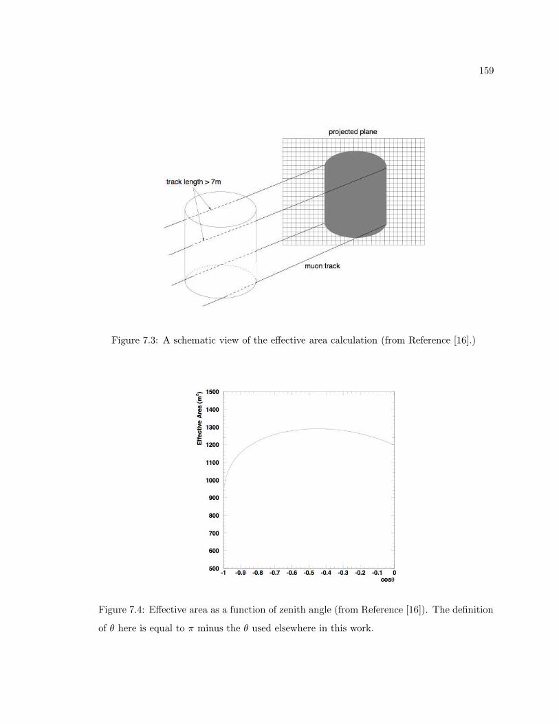
159
Figure 7.3: A schematic view of the effective area calculation (from Reference [16].)
Figure 7.4: Effective area as a function of zenith angle (from Reference [16]). The definition
of θ here is equal to π minus the θ used elsewhere in this work.
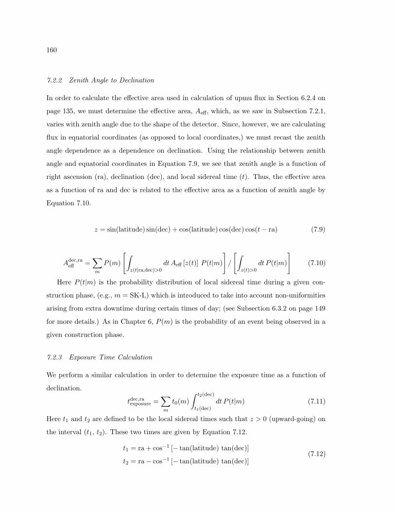
160
7.2.2 Zenith Angle to Declination
In order to calculate the effective area used in calculation of upmu flux in Section 6.2.4 on
page 135, we must determine the effective area, Aeff, which, as we saw in Subsection 7.2.1,
varies with zenith angle due to the shape of the detector. Since, however, we are calculating
flux in equatorial coordinates (as opposed to local coordinates,) we must recast the zenith
angle dependence as a dependence on declination. Using the relationship between zenith
angle and equatorial coordinates in Equation 7.9, we see that zenith angle is a function of
right ascension (ra), declination (dec), and local sidereal time (t). Thus, the effective area
as a function of ra and dec is related to the effective area as a function of zenith angle by
Equation 7.10.
z = sin(latitude) sin(dec) + cos(latitude) cos(dec) cos(t− ra) (7.9)
Adec,raeff =
∑
m
P (m)
[
∫
z(t|ra,dec)>0dtAeff [z(t)] P (t|m)
]
/
[
∫
z(t)>0dt P (t|m)
]
(7.10)
Here P (t|m) is the probability distribution of local sidereal time during a given con-
struction phase, (e.g., m = SK-I,) which is introduced to take into account non-uniformities
arising from extra downtime during certain times of day; (see Subsection 6.3.2 on page 149
for more details.) As in Chapter 6, P (m) is the probability of an event being observed in a
given construction phase.
7.2.3 Exposure Time Calculation
We perform a similar calculation in order to determine the exposure time as a function of
declination.
tdec,raexposure =
∑
m
t0(m)
∫ t2(dec)
t1(dec)dt P (t|m) (7.11)
Here t1 and t2 are defined to be the local sidereal times such that z > 0 (upward-going) on
the interval (t1, t2). These two times are given by Equation 7.12.
t1 = ra + cos−1 [− tan(latitude) tan(dec)]
t2 = ra − cos−1 [− tan(latitude) tan(dec)](7.12)
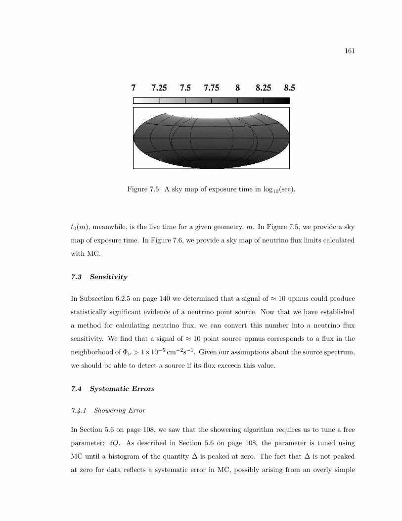
161
Figure 7.5: A sky map of exposure time in log10(sec).
t0(m), meanwhile, is the live time for a given geometry, m. In Figure 7.5, we provide a sky
map of exposure time. In Figure 7.6, we provide a sky map of neutrino flux limits calculated
with MC.
7.3 Sensitivity
In Subsection 6.2.5 on page 140 we determined that a signal of ≈ 10 upmus could produce
statistically significant evidence of a neutrino point source. Now that we have established
a method for calculating neutrino flux, we can convert this number into a neutrino flux
sensitivity. We find that a signal of ≈ 10 point source upmus corresponds to a flux in the
neighborhood of Φν > 1×10⁻⁵ cm−2s−1. Given our assumptions about the source spectrum,
we should be able to detect a source if its flux exceeds this value.
7.4 Systematic Errors
7.4.1 Showering Error
In Section 5.6 on page 108, we saw that the showering algorithm requires us to tune a free
parameter: δQ. As described in Section 5.6 on page 108, the parameter is tuned using
MC until a histogram of the quantity ∆ is peaked at zero. The fact that ∆ is not peaked
at zero for data reflects a systematic error in MC, possibly arising from an overly simple
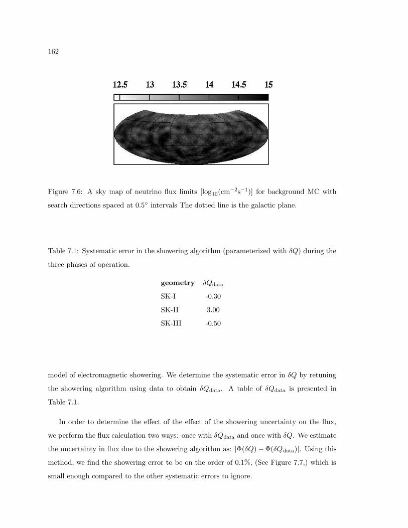
162
Figure 7.6: A sky map of neutrino flux limits [log10(cm−2s−1)] for background MC with
search directions spaced at 0.5 intervals The dotted line is the galactic plane.
Table 7.1: Systematic error in the showering algorithm (parameterized with δQ) during the
three phases of operation.
geometry δQdata
SK-I -0.30
SK-II 3.00
SK-III -0.50
model of electromagnetic showering. We determine the systematic error in δQ by retuning
the showering algorithm using data to obtain δQdata. A table of δQdata is presented in
Table 7.1.
In order to determine the effect of the effect of the showering uncertainty on the flux,
we perform the flux calculation two ways: once with δQdata and once with δQ. We estimate
the uncertainty in flux due to the showering algorithm as: |Φ(δQ) −Φ(δQdata)|. Using this
method, we find the showering error to be on the order of 0.1%, (See Figure 7.7,) which is
small enough compared to the other systematic errors to ignore.
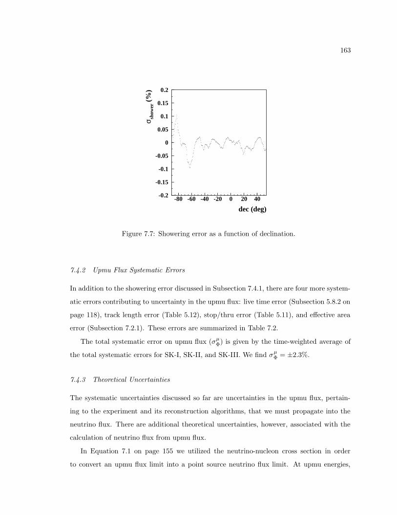
163
dec (deg)
σ show
er (
%)
-0.2
-0.15
-0.1
-0.05
0
0.05
0.1
0.15
0.2
-80 -60 -40 -20 0 20 40
Figure 7.7: Showering error as a function of declination.
7.4.2 Upmu Flux Systematic Errors
In addition to the showering error discussed in Subsection 7.4.1, there are four more system-
atic errors contributing to uncertainty in the upmu flux: live time error (Subsection 5.8.2 on
page 118), track length error (Table 5.12), stop/thru error (Table 5.11), and effective area
error (Subsection 7.2.1). These errors are summarized in Table 7.2.
The total systematic error on upmu flux (σµΦ) is given by the time-weighted average of
the total systematic errors for SK-I, SK-II, and SK-III. We find σµΦ = ±2.3%.
7.4.3 Theoretical Uncertainties
The systematic uncertainties discussed so far are uncertainties in the upmu flux, pertain-
ing to the experiment and its reconstruction algorithms, that we must propagate into the
neutrino flux. There are additional theoretical uncertainties, however, associated with the
calculation of neutrino flux from upmu flux.
In Equation 7.1 on page 155 we utilized the neutrino-nucleon cross section in order
to convert an upmu flux limit into a point source neutrino flux limit. At upmu energies,
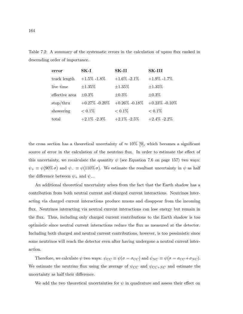
164
Table 7.2: A summary of the systematic errors in the calculation of upmu flux ranked in
descending order of importance.
error SK-I SK-II SK-III
track length +1.5% -1.8% +1.6% -2.1% +1.9% -1.7%
live time ±1.35% ±1.35% ±1.35%
effective area ±0.3% ±0.3% ±0.3%
stop/thru +0.27% -0.20% +0.26% -0.18% +0.23% -0.10%
showering < 0.1% < 0.1% < 0.1%
total +2.1% -2.3% +2.1% -2.5% +2.4% -2.2%
the cross section has a theoretical uncertainty of ≈ 10% [9], which becomes a significant
source of error in the calculation of the neutrino flux. In order to estimate the effect of
this uncertainty, we recalculate the quantity ψ (see Equation 7.6 on page 157) two ways:
ψ+ ≡ ψ(90%σ) and ψ− ≡ ψ(110%σ). We estimate the resultant uncertainty in ψ as half
the difference between ψ+ and ψ−.
An additional theoretical uncertainty arises from the fact that the Earth shadow has a
contribution from both neutral current and charged current interactions. Neutrinos inter-
acting via charged current interactions produce muons and disappear from the incoming
flux. Neutrinos interacting via neutral current interactions can lose energy but remain in
the flux. Thus, including only charged current contributions to the Earth shadow is too
optimistic since neutral current interactions reduce the flux as measured at the detector.
Including both charged and neutral current contributions, however, is too pessimistic since
some neutrinos will reach the detector even after having undergone a neutral current inter-
action.
Therefore, we calculate ψ two ways: ψCC ≡ ψ(σ = σCC) and ψNC ≡ ψ(σ = σCC +σNC).
We estimate the neutrino flux using the average of ψCC and ψCC+NC and estimate the
uncertainty as half their difference.
We add the two theoretical uncertainties for ψ in quadrature and assess their effect on
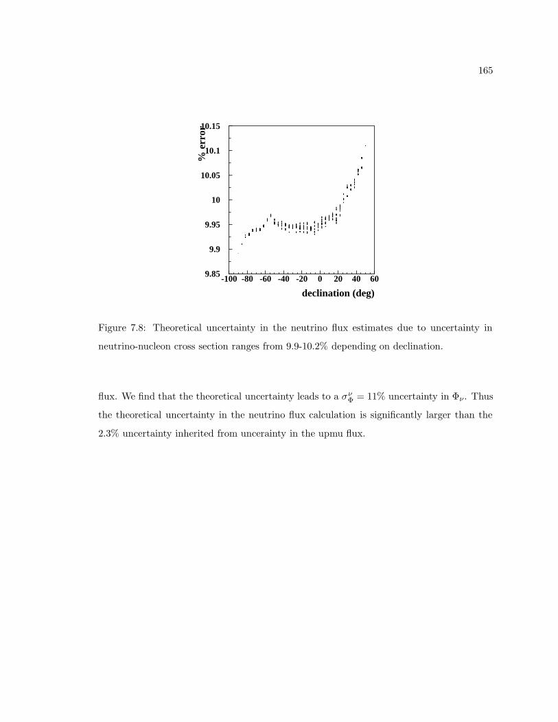
165
declination (deg)
% e
rror
9.85
9.9
9.95
10
10.05
10.1
10.15
-100 -80 -60 -40 -20 0 20 40 60
Figure 7.8: Theoretical uncertainty in the neutrino flux estimates due to uncertainty in
neutrino-nucleon cross section ranges from 9.9-10.2% depending on declination.
flux. We find that the theoretical uncertainty leads to a σνΦ = 11% uncertainty in Φν . Thus
the theoretical uncertainty in the neutrino flux calculation is significantly larger than the
2.3% uncertainty inherited from uncerainty in the upmu flux.
166
Chapter 8
RESULTS
After developing and testing the algorithm with MC—and deciding which tests to carry
out—we applied the algorithm to the data. By developing the algorithm with MC, and
deciding on the tests ahead of time, it is straightforward to assess trial factors associated
with any apparent signals. In this chapter we shall present the results of five separate tests.
The combined dataset for SK-I through SK-III is summarized in a sky map in Figure 8.1.
The blue dots are through-going muons and the red dots are showering muons. A quick
inspection by eye does not find the clustering necessary for an unambiguous signal, though
we do find statistically meaningful evidence in support of two interesting correlations.
In Section 8.1, we perform the first test, referred to as the tabula rasa search, in which
we determine the largest apparent signal in the sky, Λmax, and determine if it is higher than
usual values for the atmospheric background. The tabula rasa search is meant to identify a
point source without a priori assumptions about the most likely candidates. In this section
we present flux limits over the visible sky (dec < 54.) In Section 8.2, we look for signals from
suspected sources (identified in Section 1.7 on page 18) including magnetars, plerions,
supernova remnants, and microquasars. In Section 8.3, we look for a correlation between
upmus and UHE events detected by the Auger experiment and subsequently correlated with
active galactic nucleii. In Section 8.4, we perform a systematic GRB search for upmus
correlated with GRBs in the BATSE and Swift catalogs. Finally, in Section 8.5, we perform
a search for upmus from GRB080319B, the brightest GRB observed to date. A summary
of the results from these five tests is presented in Table 8.1.
The neutrino flux and fluence limits presented in the subsequent sections are calculated
assuming a spectral index of γ = 2. In Section 8.6, we shall assess the impact of this
assumption and describe how the limits change for a spectral index of γ = 3. We also make
a distinction between neutrinos and antineutrinos.
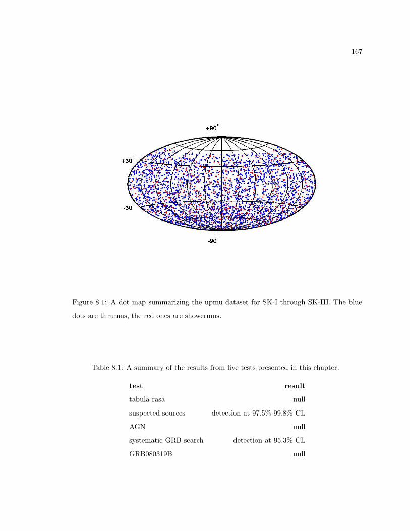
167
Figure 8.1: A dot map summarizing the upmu dataset for SK-I through SK-III. The blue
dots are thrumus, the red ones are showermus.
Table 8.1: A summary of the results from five tests presented in this chapter.
test result
tabula rasa null
suspected sources detection at 97.5%-99.8% CL
AGN null
systematic GRB search detection at 95.3% CL
GRB080319B null
168
8.1 Tabula Rasa Search
The largest signal observed at any point in the sky, Λmax = 19.1, is well below the detection
threshold.1 Thus, we assign upper limits on neutrino and upmu flux from point sources.
Upper limits on the flux of point source upmus/neutrinos as a function of declination
are presented in Figures 8.2 and 8.3 respectively. The limits worsen at higher values of
declination due to reduced exposure time. In Figure 8.4 we plot the neutrino flux limits
obtained in this study (black) alongside the an estimate of those obtained by AMANDA in
Reference [17] (red) and MACRO in Reference [18] (dotted blue.) Also included in this plot
is the expected detection threshold for this study (green). We provide sky maps of muon
and neutrino flux limits in Figures 8.5 and 8.6 respectively. A map of the likelihood ratio
Λ is provided in Figure 8.7.
8.2 Suspected Sources
8.2.1 Magnetars
In Table 1.2 on page 19 we picked four magnetars to test as neutrino point sources. The
maximum value of Λ among these candidates was 0.4, and so we observe no evidence of
neutrinos from these four magnetars. A summary of the neutrino flux limits for each
magnetar is presented in Table 8.2.
8.2.2 Plerions
In Table 1.3 on page 22 we picked four plerions to test as neutrino point sources. The
maximum value of Λ among these candidates was 0.9, and so we observe no evidence of
neutrinos from these four plerions. A summary of the neutrino flux limits for each plerion
is presented in Table 8.3.
1In fact, it is very small given the distribution of Λmax in Figure 6.11 on page 142, which prompted us torerun the algorithm using boot-strapped values for local sidereal time. The second boot-strap run yieldedΛmax = 24.9, which, while still below the detection threshold, is more typical, giving us confidence thatthe small value of Λmax = 19.1 is a reasonable fluctuation.
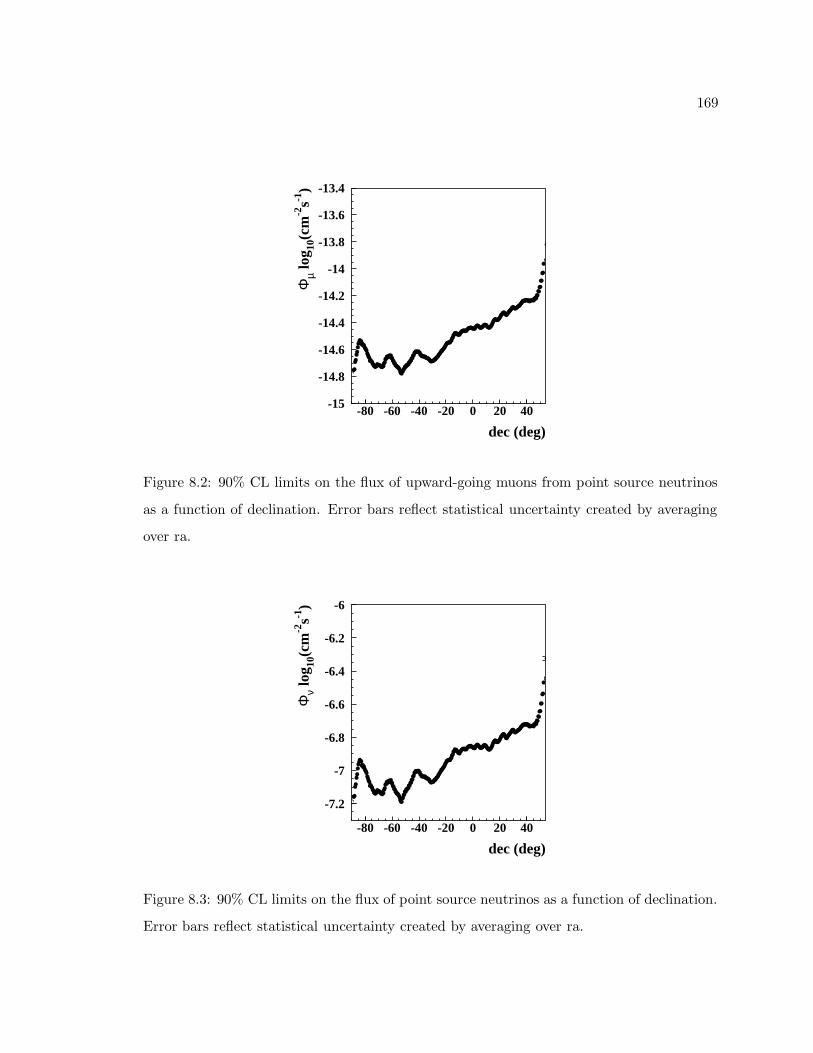
169
dec (deg)
Φµ
log 10
(cm
-2s-1
)
-15
-14.8
-14.6
-14.4
-14.2
-14
-13.8
-13.6
-13.4
-80 -60 -40 -20 0 20 40
Figure 8.2: 90% CL limits on the flux of upward-going muons from point source neutrinos
as a function of declination. Error bars reflect statistical uncertainty created by averaging
over ra.
dec (deg)
Φν
log 10
(cm
-2s-1
)
-7.2
-7
-6.8
-6.6
-6.4
-6.2
-6
-80 -60 -40 -20 0 20 40
Figure 8.3: 90% CL limits on the flux of point source neutrinos as a function of declination.
Error bars reflect statistical uncertainty created by averaging over ra.
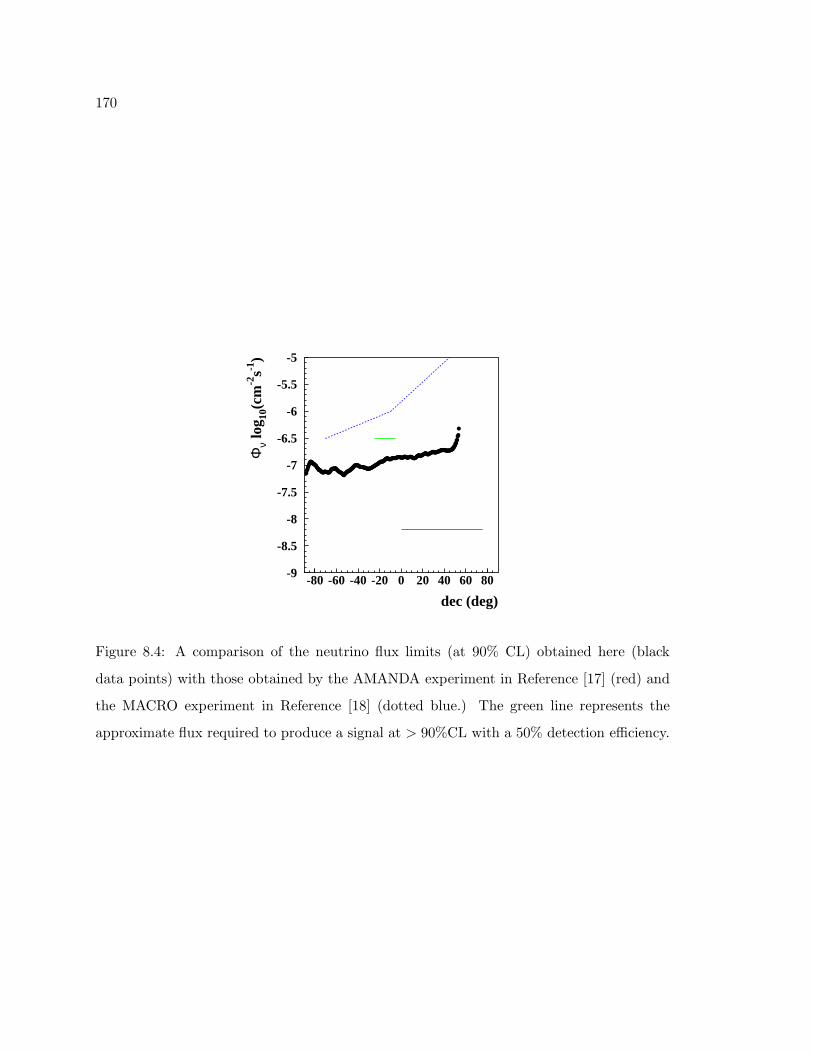
170
dec (deg)
Φν
log 10
(cm
-2s-1
)
-9
-8.5
-8
-7.5
-7
-6.5
-6
-5.5
-5
-80 -60 -40 -20 0 20 40 60 80
Figure 8.4: A comparison of the neutrino flux limits (at 90% CL) obtained here (black
data points) with those obtained by the AMANDA experiment in Reference [17] (red) and
the MACRO experiment in Reference [18] (dotted blue.) The green line represents the
approximate flux required to produce a signal at > 90%CL with a 50% detection efficiency.
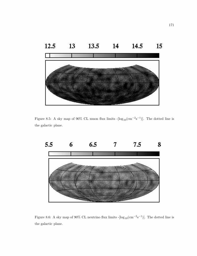
171
Figure 8.5: A sky map of 90% CL muon flux limits -[log10(cm−2s−1)]. The dotted line is
the galactic plane.
Figure 8.6: A sky map of 90% CL neutrino flux limits -[log10(cm−2s−1)]. The dotted line is
the galactic plane.
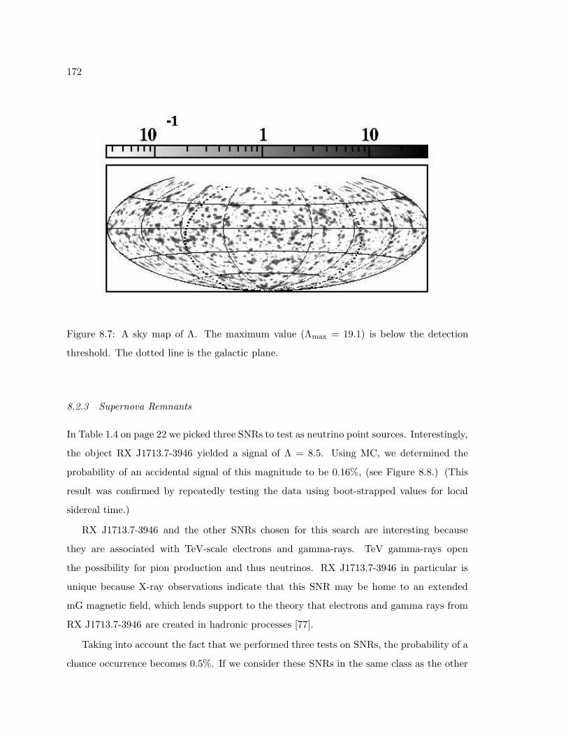
172
Figure 8.7: A sky map of Λ. The maximum value (Λmax = 19.1) is below the detection
threshold. The dotted line is the galactic plane.
8.2.3 Supernova Remnants
In Table 1.4 on page 22 we picked three SNRs to test as neutrino point sources. Interestingly,
the object RX J1713.7-3946 yielded a signal of Λ = 8.5. Using MC, we determined the
probability of an accidental signal of this magnitude to be 0.16%, (see Figure 8.8.) (This
result was confirmed by repeatedly testing the data using boot-strapped values for local
sidereal time.)
RX J1713.7-3946 and the other SNRs chosen for this search are interesting because
they are associated with TeV-scale electrons and gamma-rays. TeV gamma-rays open
the possibility for pion production and thus neutrinos. RX J1713.7-3946 in particular is
unique because X-ray observations indicate that this SNR may be home to an extended
mG magnetic field, which lends support to the theory that electrons and gamma rays from
RX J1713.7-3946 are created in hadronic processes [77].
Taking into account the fact that we performed three tests on SNRs, the probability of a
chance occurrence becomes 0.5%. If we consider these SNRs in the same class as the other
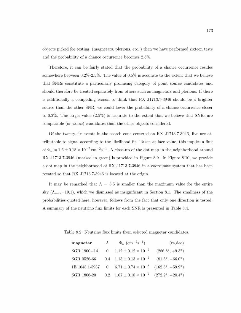
173
objects picked for testing, (magnetars, plerions, etc.,) then we have performed sixteen tests
and the probability of a chance occurrence becomes 2.5%.
Therefore, it can be fairly stated that the probability of a chance occurrence resides
somewhere between 0.2%-2.5%. The value of 0.5% is accurate to the extent that we believe
that SNRs constitute a particularly promising category of point source candidates and
should therefore be treated separately from others such as magnetars and plerions. If there
is additionally a compelling reason to think that RX J1713.7-3946 should be a brighter
source than the other SNR, we could lower the probability of a chance occurrence closer
to 0.2%. The larger value (2.5%) is accurate to the extent that we believe that SNRs are
comparable (or worse) candidates than the other objects considered.
Of the twenty-six events in the search cone centered on RX J1713.7-3946, five are at-
tributable to signal according to the likelihood fit. Taken at face value, this implies a flux
of Φν ≈ 1.6 ± 0.18 × 10⁻⁷ cm−2s−1. A close-up of the dot map in the neighborhood around
RX J1713.7-3946 (marked in green) is provided in Figure 8.9. In Figure 8.10, we provide
a dot map in the neighborhood of RX J1713.7-3946 in a coordinate system that has been
rotated so that RX J1713.7-3946 is located at the origin.
It may be remarked that Λ = 8.5 is smaller than the maximum value for the entire
sky (Λmax=19.1), which we dismissed as insignificant in Section 8.1. The smallness of the
probabilities quoted here, however, follows from the fact that only one direction is tested.
A summary of the neutrino flux limits for each SNR is presented in Table 8.4.
Table 8.2: Neutrino flux limits from selected magnetar candidates.
magnetar Λ Φν (cm−2s−1) (ra,dec)
SGR 1900+14 0 1.12 ± 0.12 × 10⁻⁷ (286.8,+9.3)
SGR 0526-66 0.4 1.15 ± 0.13 × 10⁻⁷ (81.5,−66.0)
1E 1048.1-5937 0 6.71 ± 0.74 × 10⁻⁸ (162.5,−59.9)
SGR 1806-20 0.2 1.67 ± 0.18 × 10⁻⁷ (272.2,−20.4)
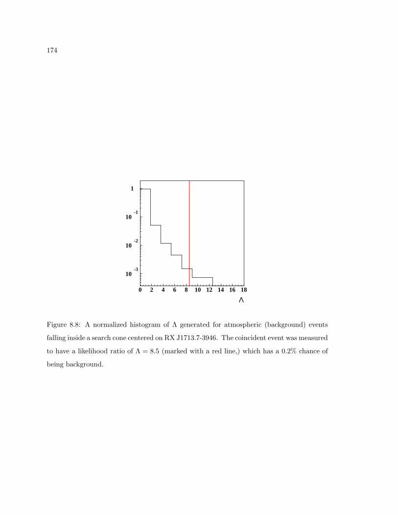
174
Λ
10-3
10-2
10-1
1
0 2 4 6 8 10 12 14 16 18
Figure 8.8: A normalized histogram of Λ generated for atmospheric (background) events
falling inside a search cone centered on RX J1713.7-3946. The coincident event was measured
to have a likelihood ratio of Λ = 8.5 (marked with a red line,) which has a 0.2% chance of
being background.
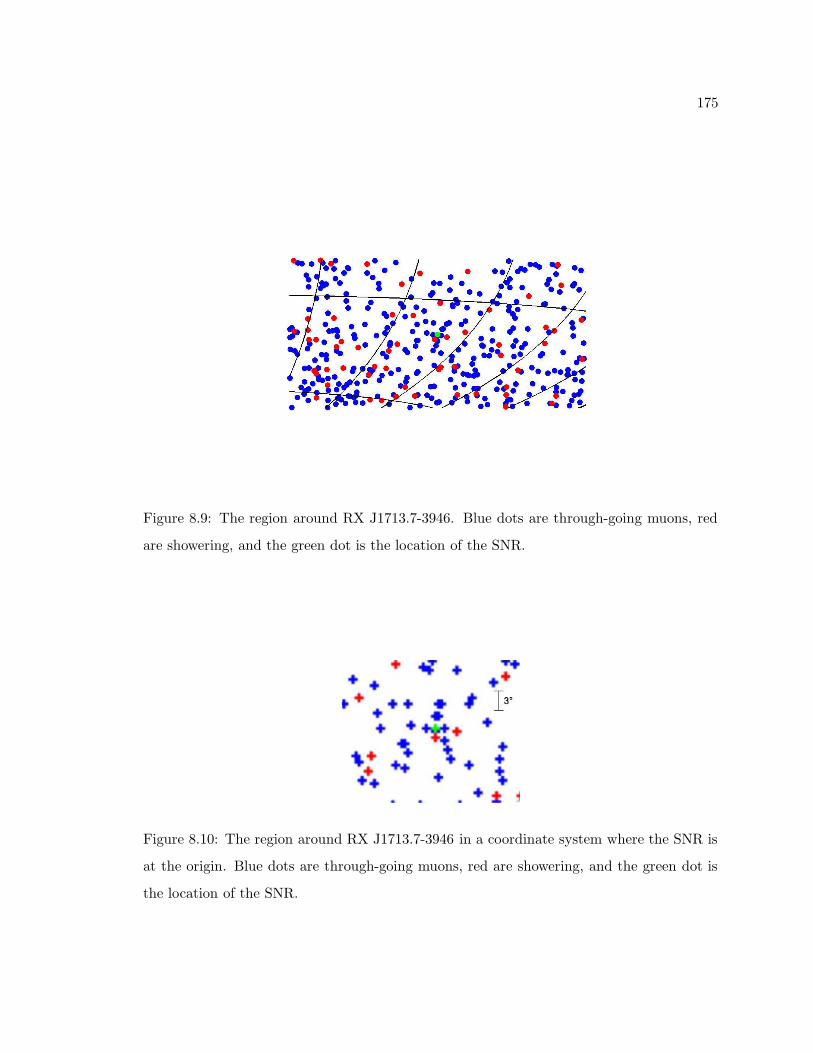
175
Figure 8.9: The region around RX J1713.7-3946. Blue dots are through-going muons, red
are showering, and the green dot is the location of the SNR.
Figure 8.10: The region around RX J1713.7-3946 in a coordinate system where the SNR is
at the origin. Blue dots are through-going muons, red are showering, and the green dot is
the location of the SNR.
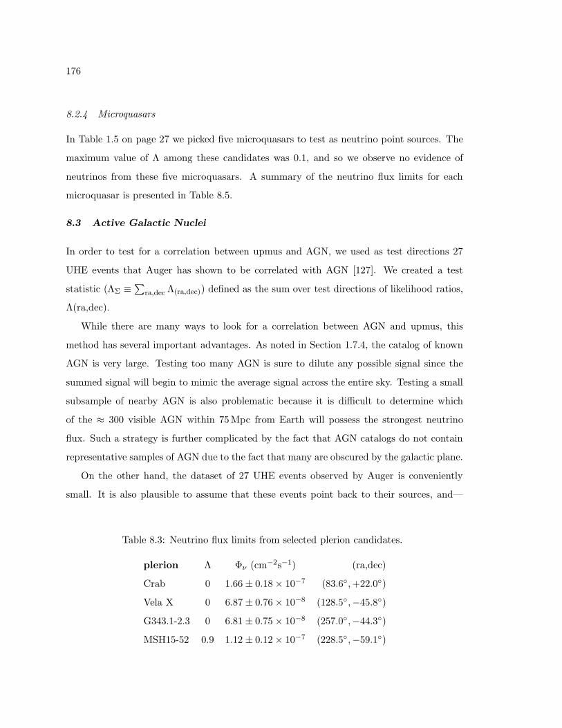
176
8.2.4 Microquasars
In Table 1.5 on page 27 we picked five microquasars to test as neutrino point sources. The
maximum value of Λ among these candidates was 0.1, and so we observe no evidence of
neutrinos from these five microquasars. A summary of the neutrino flux limits for each
microquasar is presented in Table 8.5.
8.3 Active Galactic Nuclei
In order to test for a correlation between upmus and AGN, we used as test directions 27
UHE events that Auger has shown to be correlated with AGN [127]. We created a test
statistic (ΛΣ ≡∑ra,dec Λ(ra,dec)) defined as the sum over test directions of likelihood ratios,
Λ(ra,dec).
While there are many ways to look for a correlation between AGN and upmus, this
method has several important advantages. As noted in Section 1.7.4, the catalog of known
AGN is very large. Testing too many AGN is sure to dilute any possible signal since the
summed signal will begin to mimic the average signal across the entire sky. Testing a small
subsample of nearby AGN is also problematic because it is difficult to determine which
of the ≈ 300 visible AGN within 75Mpc from Earth will possess the strongest neutrino
flux. Such a strategy is further complicated by the fact that AGN catalogs do not contain
representative samples of AGN due to the fact that many are obscured by the galactic plane.
On the other hand, the dataset of 27 UHE events observed by Auger is conveniently
small. It is also plausible to assume that these events point back to their sources, and—
Table 8.3: Neutrino flux limits from selected plerion candidates.
plerion Λ Φν (cm−2s−1) (ra,dec)
Crab 0 1.66 ± 0.18 × 10⁻⁷ (83.6,+22.0)
Vela X 0 6.87 ± 0.76 × 10⁻⁸ (128.5,−45.8)
G343.1-2.3 0 6.81 ± 0.75 × 10⁻⁸ (257.0,−44.3)
MSH15-52 0.9 1.12 ± 0.12 × 10⁻⁷ (228.5,−59.1)
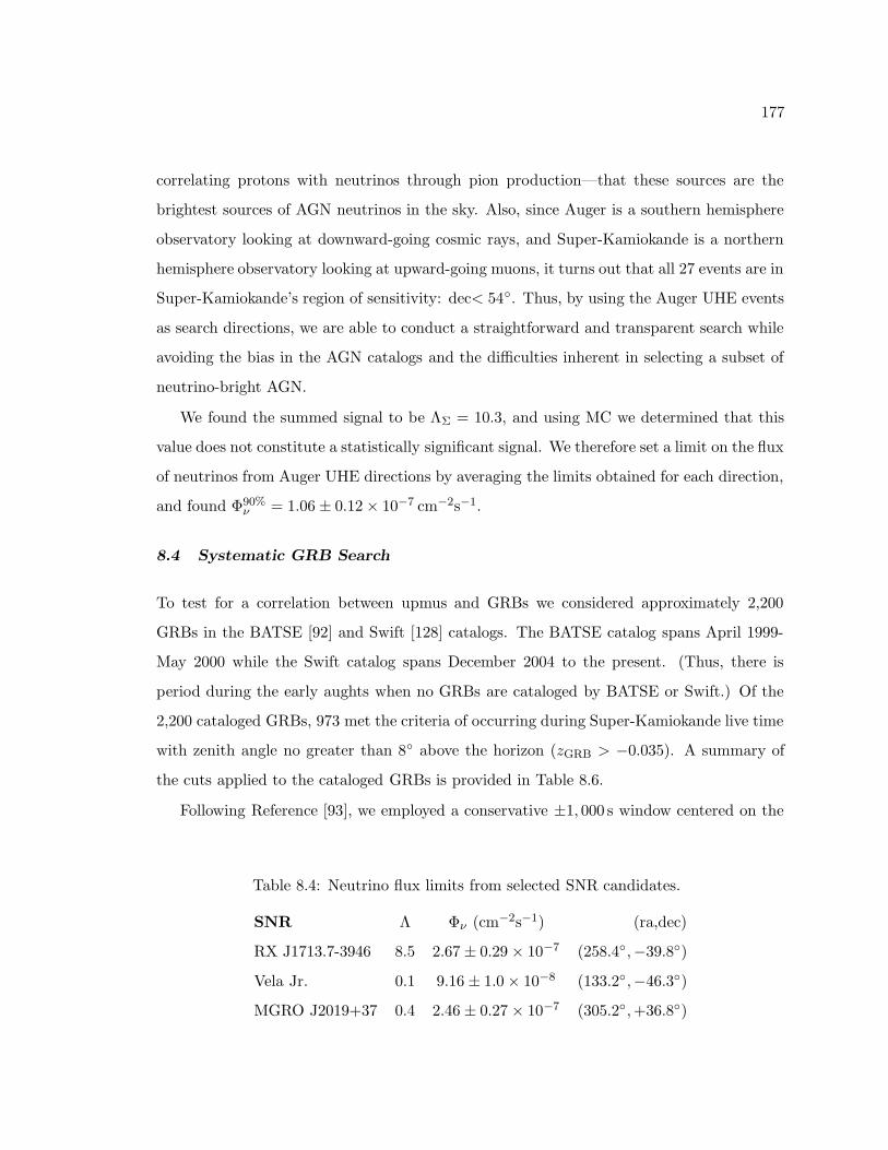
177
correlating protons with neutrinos through pion production—that these sources are the
brightest sources of AGN neutrinos in the sky. Also, since Auger is a southern hemisphere
observatory looking at downward-going cosmic rays, and Super-Kamiokande is a northern
hemisphere observatory looking at upward-going muons, it turns out that all 27 events are in
Super-Kamiokande’s region of sensitivity: dec< 54. Thus, by using the Auger UHE events
as search directions, we are able to conduct a straightforward and transparent search while
avoiding the bias in the AGN catalogs and the difficulties inherent in selecting a subset of
neutrino-bright AGN.
We found the summed signal to be ΛΣ = 10.3, and using MC we determined that this
value does not constitute a statistically significant signal. We therefore set a limit on the flux
of neutrinos from Auger UHE directions by averaging the limits obtained for each direction,
and found Φ90%ν = 1.06 ± 0.12 × 10⁻⁷ cm−2s−1.
8.4 Systematic GRB Search
To test for a correlation between upmus and GRBs we considered approximately 2,200
GRBs in the BATSE [92] and Swift [128] catalogs. The BATSE catalog spans April 1999-
May 2000 while the Swift catalog spans December 2004 to the present. (Thus, there is
period during the early aughts when no GRBs are cataloged by BATSE or Swift.) Of the
2,200 cataloged GRBs, 973 met the criteria of occurring during Super-Kamiokande live time
with zenith angle no greater than 8 above the horizon (zGRB > −0.035). A summary of
the cuts applied to the cataloged GRBs is provided in Table 8.6.
Following Reference [93], we employed a conservative ±1, 000 s window centered on the
Table 8.4: Neutrino flux limits from selected SNR candidates.
SNR Λ Φν (cm−2s−1) (ra,dec)
RX J1713.7-3946 8.5 2.67 ± 0.29 × 10⁻⁷ (258.4,−39.8)
Vela Jr. 0.1 9.16 ± 1.0 × 10⁻⁸ (133.2,−46.3)
MGRO J2019+37 0.4 2.46 ± 0.27 × 10⁻⁷ (305.2,+36.8)
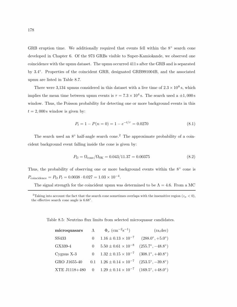
178
GRB eruption time. We additionally required that events fell within the 8 search cone
developed in Chapter 6. Of the 973 GRBs visible to Super-Kamiokande, we observed one
coincidence with the upmu dataset. The upmu occurred 411 s after the GRB and is separated
by 3.4. Properties of the coincident GRB, designated GRB991004B, and the associated
upmu are listed in Table 8.7.
There were 3,134 upmus considered in this dataset with a live time of 2.3× 10⁸ s, which
implies the mean time between upmu events is τ = 7.3 × 10⁴ s. The search used a ±1, 000 s
window. Thus, the Poisson probability for detecting one or more background events in this
t = 2, 000 s window is given by:
Pt = 1 − P (n = 0) = 1 − e−t/τ = 0.0270 (8.1)
The search used an 8 half-angle search cone.2 The approximate probability of a coin-
cident background event falling inside the cone is given by:
PΩ = Ωcone/ΩSK = 0.043/11.37 = 0.00375 (8.2)
Thus, the probability of observing one or more background events within the 8 cone is
Pcoincidence = PΩ Pt = 0.0038 · 0.027 = 1.03 × 10⁻⁴.
The signal strength for the coincident upmu was determined to be Λ = 4.6. From a MC
2Taking into account the fact that the search cone sometimes overlaps with the insensitive region (zµ < 0),the effective search cone angle is 6.68.
Table 8.5: Neutrino flux limits from selected microquasar candidates.
microquasars Λ Φν (cm−2s−1) (ra,dec)
SS433 0 1.16 ± 0.13 × 10⁻⁷ (288.0,+5.0)
GX339-4 0 5.50 ± 0.61 × 10⁻⁸ (255.7,−48.8)
Cygnus X-3 0 1.32 ± 0.15 × 10⁻⁷ (308.1,+40.8)
GRO J1655-40 0.1 1.26 ± 0.14 × 10⁻⁷ (253.5,−39.8)
XTE J1118+480 0 1.29 ± 0.14 × 10⁻⁷ (169.5,+48.0)
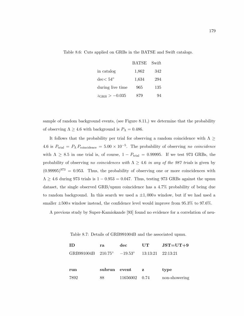
179
Table 8.6: Cuts applied on GRBs in the BATSE and Swift catalogs.
BATSE Swift
in catalog 1,862 342
dec< 54 1,634 294
during live time 965 135
zGRB > −0.035 879 94
sample of random background events, (see Figure 8.11,) we determine that the probability
of observing Λ ≥ 4.6 with background is PΛ = 0.486.
It follows that the probability per trial for observing a random coincidence with Λ ≥4.6 is Ptrial = PΛ Pcoincidence = 5.00 × 10⁻⁵. The probability of observing no coincidence
with Λ ≥ 8.5 in one trial is, of course, 1 − Ptrial = 0.99995. If we test 973 GRBs, the
probability of observing no coincidences with Λ ≥ 4.6 in any of the 987 trials is given by
(0.99995)973 = 0.953. Thus, the probability of observing one or more coincidences with
Λ ≥ 4.6 during 973 trials is 1 − 0.953 = 0.047. Thus, testing 973 GRBs against the upmu
dataset, the single observed GRB/upmu coincidence has a 4.7% probability of being due
to random background. In this search we used a ±1, 000 s window, but if we had used a
smaller ±500 s window instead, the confidence level would improve from 95.3% to 97.6%.
A previous study by Super-Kamiokande [93] found no evidence for a correlation of neu-
Table 8.7: Details of GRB991004B and the associated upmu.
ID ra dec UT JST=UT+9
GRB991004B 210.75 −19.53 13:13:21 22:13:21
run subrun event z type
7892 88 11656002 0.74 non-showering
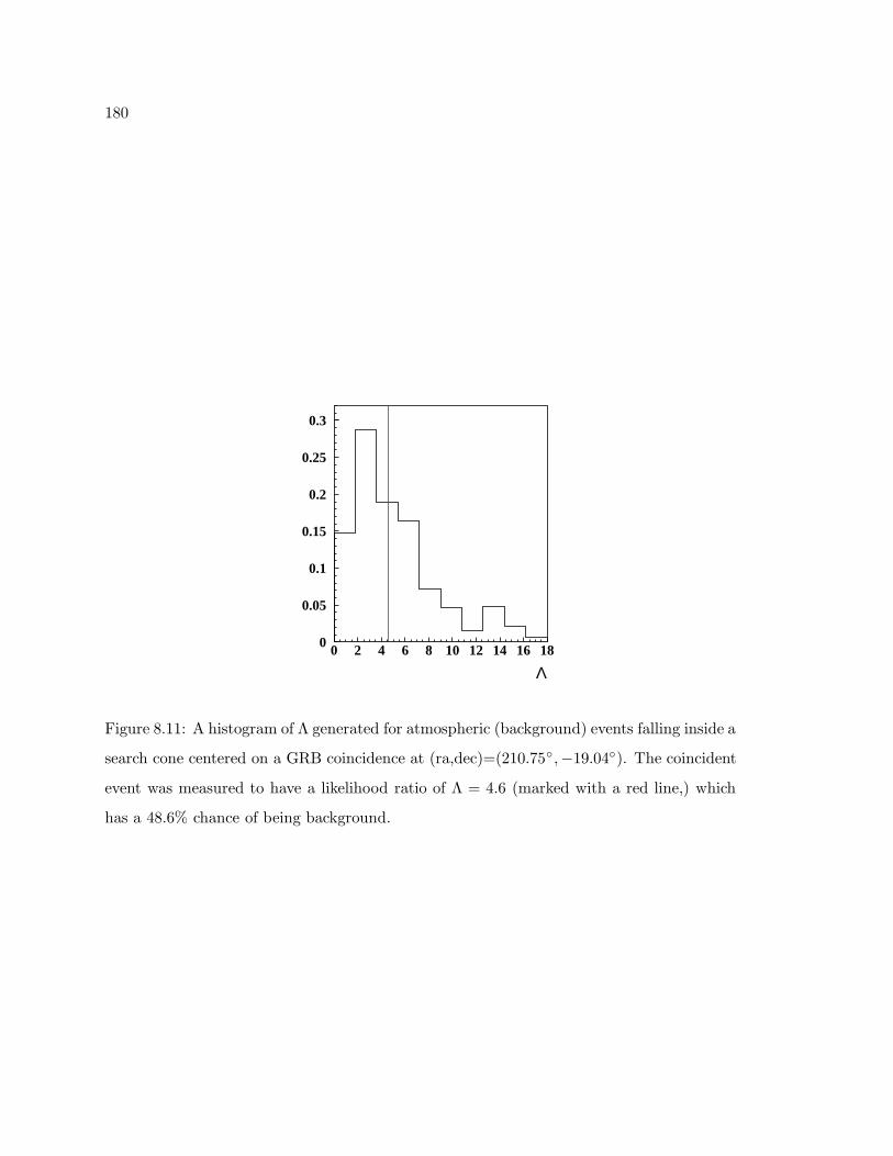
180
Λ
0
0.05
0.1
0.15
0.2
0.25
0.3
0 2 4 6 8 10 12 14 16 18
Figure 8.11: A histogram of Λ generated for atmospheric (background) events falling inside a
search cone centered on a GRB coincidence at (ra,dec)=(210.75 ,−19.04). The coincident
event was measured to have a likelihood ratio of Λ = 4.6 (marked with a red line,) which
has a 48.6% chance of being background.
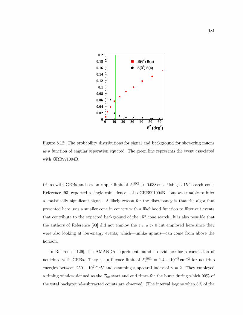
181
B(θ2) B(n)
S(θ2) S(n)
θ2 (deg2)
0
0.02
0.04
0.06
0.08
0.1
0.12
0.14
0.16
0.18
0.2
0 10 20 30 40 50 60
Figure 8.12: The probability distributions for signal and background for showering muons
as a function of angular separation squared. The green line represents the event associated
with GRB991004B.
trinos with GRBs and set an upper limit of F 90%ν > 0.038 cm. Using a 15 search cone,
Reference [93] reported a single coincidence—also GRB991004B—but was unable to infer
a statistically significant signal. A likely reason for the discrepancy is that the algorithm
presented here uses a smaller cone in concert with a likelihood function to filter out events
that contribute to the expected background of the 15 cone search. It is also possible that
the authors of Reference [93] did not employ the zGRB > 0 cut employed here since they
were also looking at low-energy events, which—unlike upmus—can come from above the
horizon.
In Reference [129], the AMANDA experiment found no evidence for a correlation of
neutrinos with GRBs. They set a fluence limit of F 90%ν = 1.4 × 10⁻⁵ cm−2 for neutrino
energies between 250 − 107 GeV and assuming a spectral index of γ = 2. They employed
a timing window defined as the T90 start and end times for the burst during which 90% of
the total background-subtracted counts are observed. (The interval begins when 5% of the
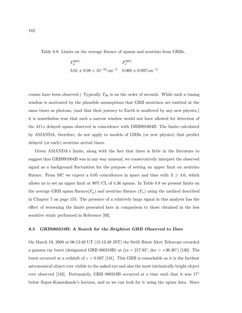
182
Table 8.8: Limits on the average fluence of upmus and neutrino from GRBs.
F 90%µ F 90%
ν
3.61 ± 0.08 × 10⁻¹⁰ cm−2 0.060 ± 0.007 cm−2
counts have been observed.) Typically T90 is on the order of seconds. While such a timing
window is motivated by the plausible assumptions that GRB neutrinos are emitted at the
same times as photons, (and that their journey to Earth is unaltered by any new physics,)
it is nonetheless true that such a narrow window would not have allowed for detection of
the 411 s delayed upmu observed in coincidence with GRB991004B. The limits calculated
by AMANDA, therefore, do not apply to models of GRBs (or new physics) that predict
delayed (or early) neutrino arrival times.
Given AMANDA’s limits, along with the fact that there is little in the literature to
suggest that GRB991004B was in any way unusual, we conservatively interpret the observed
signal as a background fluctuation for the purpose of setting an upper limit on neutrino
fluence. From MC we expect a 0.05 coincidences in space and time with Λ ≥ 4.6, which
allows us to set an upper limit at 90% CL of 4.36 upmus. In Table 8.8 we present limits on
the average GRB upmu fluence(Fµ) and neutrino fluence (Fν) using the method described
in Chapter 7 on page 155. The presence of a relatively large signal in this analysis has the
effect of worsening the limits presented here in comparison to those obtained in the less
sensitive study performed in Reference [93].
8.5 GRB080319B: A Search for the Brightest GRB Observed to Date
On March 19, 2008 at 06:12:49 UT (15:12:49 JST) the Swift Burst Alert Telescope recorded
a gamma ray burst (designated GRB 080319B) at (ra = 217.93,dec = +36.30) [130]. The
burst occurred at a redshift of z = 0.937 [131]. This GRB is remarkable as it is the farthest
astronomical object ever visible to the naked eye and also the most intrinsically bright object
ever observed [132]. Fortunately, GRB 080319B occurred at a time such that it was 17
below Super-Kamiokande’s horizon, and so we can look for it using the upmu data. Since
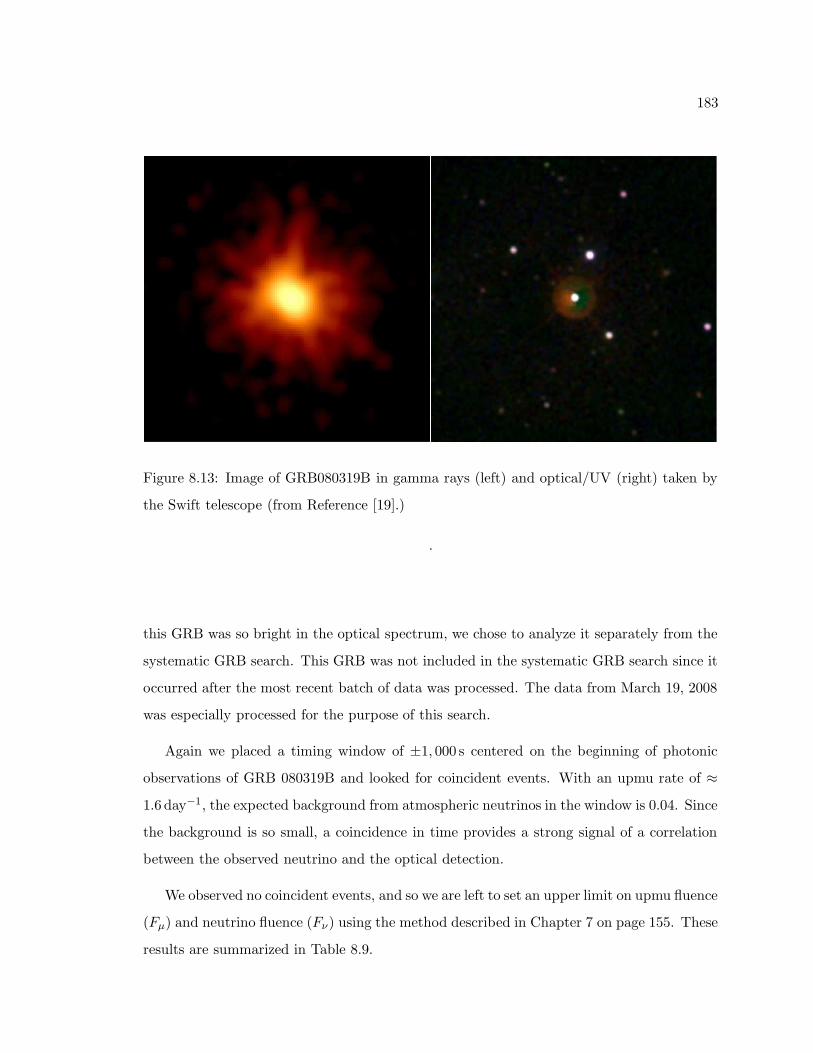
183
Figure 8.13: Image of GRB080319B in gamma rays (left) and optical/UV (right) taken by
the Swift telescope (from Reference [19].)
.
this GRB was so bright in the optical spectrum, we chose to analyze it separately from the
systematic GRB search. This GRB was not included in the systematic GRB search since it
occurred after the most recent batch of data was processed. The data from March 19, 2008
was especially processed for the purpose of this search.
Again we placed a timing window of ±1, 000 s centered on the beginning of photonic
observations of GRB 080319B and looked for coincident events. With an upmu rate of ≈1.6 day−1, the expected background from atmospheric neutrinos in the window is 0.04. Since
the background is so small, a coincidence in time provides a strong signal of a correlation
between the observed neutrino and the optical detection.
We observed no coincident events, and so we are left to set an upper limit on upmu fluence
(Fµ) and neutrino fluence (Fν) using the method described in Chapter 7 on page 155. These
results are summarized in Table 8.9.
184
Table 8.9: Limits on the fluence of upmus and neutrinos from GRB090319B.
F90%µ F90%
ν
1.92 ± 0.04 × 10⁻⁷ cm−2 16 ± 1.7 cm−2
8.6 Assessing Model Assumptions
8.6.1 Sensitivity to the Spectral Index
In Chapter 1 we argued that neutrino point sources are plausibly modeled with power law
spectra with a spectral index of γ = 2. Then in Chapter 7, we saw that some assumption
about the source spectrum is necessary in order to estimate the neutrino flux from the ob-
served muon flux. Indeed, it is standard in neutrino astronomy literature to quote neutrino
flux with an assumed spectral index of γ = 2. In this subsection we assess how the neutrino
flux limits change when we instead assume a spectral index of γ = 3.
In Figure 8.14 we plot the neutrino flux as a function of declination as in Figure 8.3 on
page 169, but instead assuming an atypical spectral index of γ = 3. The algorithm performs
slightly worse with γ = 3 compared to γ = 2 due to the widened point spread function and
the reduction in showering muons in the signal distribution, but these effects are trivial
in comparison to the effect arising from reduced neutrino-nucleon cross section at lower
energies. The limits obtained with γ = 3 are worse by about three orders of magnitude.
We thus conclude that the numerical estimates of neutrino flux are extremely sensitive
to assumptions about the source spectrum. While it is necessary to make an assumption
about the nature of the source—and the γ = 2 power law spectrum is certainly a useful stan-
dard assumption—it should be noted that until we know more about point source spectra,
numerical limits on neutrino flux are best suited for comparison between experiments.
8.6.2 Antineutrinos
So far our flux calculations have all been carried out using cross sections and muon range
probabilities for νµ and µ− respectively—not νµ and µ+. As energy decreases, however, the
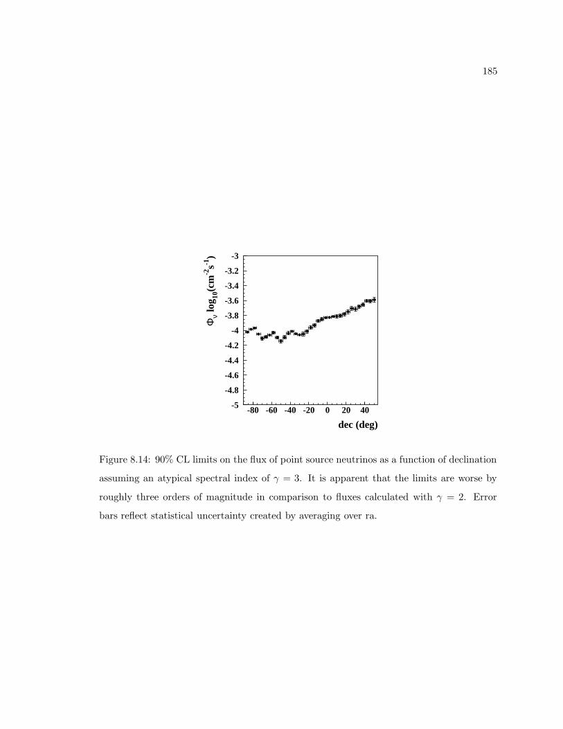
185
dec (deg)
Φν
log 10
(cm
-2s-1
)
-5
-4.8
-4.6
-4.4
-4.2
-4
-3.8
-3.6
-3.4
-3.2
-3
-80 -60 -40 -20 0 20 40
Figure 8.14: 90% CL limits on the flux of point source neutrinos as a function of declination
assuming an atypical spectral index of γ = 3. It is apparent that the limits are worse by
roughly three orders of magnitude in comparison to fluxes calculated with γ = 2. Error
bars reflect statistical uncertainty created by averaging over ra.
186
cross section for νµ-nucleon scattering becomes smaller in comparison to the cross section
for νµ-nucleon scattering. This is due to the fact that neutrinos are left-handed while
antineutrinos are right-handed.
At energies around 1GeV neutrinos interact with down quarks and antineutrinos interact
with up quarks as in Equation 8.3 and Equation 8.4 respectively.
νµ + d→ µ− + u (8.3)
νµ + u→ µ+ + d (8.4)
Due to the V −A character of the weak force, the interaction in Equation 8.3 will only take
place if u and νµ are both left-handed. In the center of mass frame the spin vectors are
antiparallel, and the resultant amplitude is an s wave (with no angular dependence.) In
Equation 8.4, however, ν is necessarily right-handed while u is left-handed. In the center of
mass frame the spin vectors are parallel, and so the resultant amplitude is a p wave, (which
depends on scattering angle.) Transforming from the center of mass frame to the lab frame,
the angular dependence of the p wave can be recharacterized as an energy dependence,
which has the effect of diminishing the antineutrino-nucleon cross section at lower energies
relative to the neutrino-nucleon cross section.
Numerically, antineutrino flux limits are 1.32 times higher than neutrino flux limits
(given our assumptions about the source spectrum and averaging over the upmu energy
spectrum.) The difference in muon range probabilities is marginal.
187
Chapter 9
CONCLUSIONS
We have constructed an algorithm for the purpose of detecting neutrino point sources.
The algorithm was designed to be maximally efficient, using all available information. We
find that this algorithm is more sensitive by a factor of two in comparison to previous point
source searches.
Using the algorithm, we conducted five tests. Our tabula rasa search found no evidence
for an unexpected point source. We set limits on neutrino flux at 90% CL as low as
6× 10⁻⁸ cm−2s−1 for declinations less than +54. While not competitive with AMANDA’s
limits, these limits are among the best for dec < 0.
In a test of suspected sources, we looked for signals from 16 predetermined objects
classified as potential neutrino point sources. These objects included magnetars, plerions,
supernova remnants, and microquasars. Of the 16 objects tested, we found one to have a
high enough signal to warrant interest. In particular, the SNR RX J1713.7-3946 was found
to possess a signal at between 97.5%-99.8% CL depending on how one assesses the trial
factors.
Using a recent discovery by the Auger experiment correlating UHE cosmic rays with
AGN, we looked for a correlation of upmus with the brightest AGN. We found no evidence for
a correlation and set a limit on the average neutrino flux from Auger UHE event directions,
Φ90%ν = 1.06 ± 0.12 × 10⁻⁷ cm−2s−1.
We performed a systematic search for correlations of upmus with GRBs in the BATSE
and Swift catalogs. We found one coincidence (with GRB991004D,) which constitutes a
signal at 95.3% CL. We set a limit on average GRB neutrino fluence, F 90%ν = 0.060 ±
0.007 cm−2.
Finally, we looked for coincident upmus from GRB080319B, the brightest GRB ob-
served to date. Finding no coincidences, we set an upper limit on neutrino fluence from
188
GRB080319B, F 90%ν = 16 ± 1.7 cm−2.
Interpreted charitably, neither of the signals observed in this work constitute unam-
biguous evidence for neutrinos from distant sources. The observation of a coincidence
with GRB991004D must be reconciled with the low limits on GRB neutrino fluence set
by AMANDA. Unless there is something unusual found about GRB991004D—or we pos-
tulate new physics causing GRB neutrinos to arrive hundreds of seconds after their photon
brethren—the observed correlation is for now best interpreted as a chance coincidence with
an atmospheric neutrino.
In the case of RX J1713.7-3946, AMANDA can be of no assistance, since they are not
sensitive to the right part of the sky (dec = −39.8.) Future northern hemisphere detectors
such as ANTARES, however, should be able to assess the neutrino flux from RX J1713.7-
3946 in the near future with improved sensitivity.
Whether or not future experiments can observe a signal from RX J1713.7-3946 consistent
with the observations herein, the field of neutrino astronomy is likely to provide great insight
into high energy objects both galactic and extragalactic in origin. With new experiments
planned and in progress, we can expect these results in the foreseeable future. In the broader
field of UHE astronomy, a new generation of experiments based on the detection of gamma
rays, cosmic rays, and gravity waves—combined with neutrino astronomy—should begin to
elucidate the high energy universe. The author predicts that the subsequent decade or two
will be good ones for the young field of UHE astronomy.
189
BIBLIOGRAPHY
[1] A. M. Hillas, “The origin of ultra-high-energy cosmic rays,” Annual Review ofAstronomy and Astrophysics 22 (2004) 425–44.
[2] T. Gaisser, “The cosmic-ray spectrum: From the knee to the ankle,” Journal ofPhysics: Conference Series 47 (2006) 15–20.http://www.iop.org/EJ/article/1742-6596/47/1/002/jpconf6_47_002.pdf.
[3] J. Hester and A. L. A. S. University) NASA, ESA,http://hubblesite.org/gallery/album/entire_collection/pr2005037a/.
[4] NASA/CXC/Rutgers/J.Warren and J.Hughes and others.
[5] STScI., “Hubble provides multiple views of how to feed a black hole.” Press release:Space Telescope Science Institute. March 14, 1998.
[6] A. Fruchter, (STScI), and NASA.http://hubblesite.org/newscenter/archive/releases/1999/09/.
[7] V. Agrawal et al., “Atmospheric neutrino flux above 1GeV,” Physical Review D 53(1996). 3.
[8] R. Gandhi et al. Physical Review D 58 (1998) 093009–0093024.
[9] R. Gandhi et al., “Ultrahigh-energy neutrino interactions,” Astroparticle Physics 5(1996) hep-ph/9512364. 81.
[10] The Super-K Collaboration, “The super-kamiokande detector,” NuclearInstruments and Methods in Physics Research A 501 (2003) 418–462.
[11] H. Berns, “Od/he burst trigger + no od tdc histograms,” tech. rep. http://neutrino.phys.washington.edu/~superk/onsite/MONITOR/HIST/TRGhist.html.
[12] S. Desai, High Energy Neutrino Astronomy with Super-Kamiokande. PhD thesis,Boston University, Boston, MA, 2004.http://www-sk.icrr.u-tokyo.ac.jp/sk/pub/desai.pdf.
[13] W.-M. Yao et al. J. Phys. G 33 (2006) 1,http://pdg.lbl.gov/2007/reviews/passagerpp.pdf.
190
[14] S. Desai, “Study of tev neutrinos with upward showering muons insuper-kamiokande,”. submitted to Astroparticle Physics.
[15] Y. Shiraishi, Super-Kamiokande Atmospheric Neutrino Analysis ofMatter-Dependent Neutrino Oscillation Models. PhD thesis, University ofWashington, Seattle, WA, 2006.
[16] C. Saji, Study of Upward-Going Muons in Super-Kamiokande. PhD thesis, NiigataUniversity, 2002. http://www-sk.icrr.u-tokyo.ac.jp/sk/pub/sajithesis.pdf.
[17] The IceCube Collaboration, A. Achterberg et al. astro-ph/0611063.
[18] Ambrosio et al., “Neutrino astronomy with the macro detector,” The AstrophysicalJournal 546 (2001) 1038–1054.
[19] The Swift Collaboration, Immler et al.http://www.nasa.gov/images/content/218810main_grb_20080320_HI.jpg, 2008.
[20] B. Zhang et al., “High-energy neutrinos from magnetars,” The Astrophysical Journal595 (2003) 346–351.
[21] McGill Pulsar Group Collaborationhttp://www.physics.mcgill.ca/~pulsar/magnetar/main.html, 2007.
[22] G. B. Giacani et al. ApJ 121 (2001) 3133.
[23] A. A. Abdo et al., “Tev gamma-ray sources from a survey of the galactic plane withmilagro,” The Astrophysical Journal 664 (2007) L91–L94.
[24] S. Aiello et al., “Sensitivity of an underwater cerenkov telescope to tev neutrinosfrom galactic microquasars,” http://arxiv.org/pdf/astro-ph/0608053.
[25] The IceCube Collaboration, O. Botner, “The IceCube Neutrino Observatory,”Nuclear Physics B 143 (June, 2005) 367–370.
[26] A. Kappes, “Km3net: A next generation neutrino telescope in the mediterraneansea,” http://arxiv.org/pdf/0711.0563.
[27] J. Wilkes, “Uno,” http://arxiv.org/pdf/hep-ex/0507097.
[28] M. Shiozawa, “Hyper-kamiokande project.” Talk at 2001 JHF-Kamioka NuWorkshop, http://neutrino.kek.jp/jhfnu/workshop2/ohp/shiozawa.pdf.
191
[29] The IceCube Collaboration, “Fy 2007 budget request to congress,”.http://nsf.gov/od/opp/budget/07_budget/mrf_icecube_07.pdf.
[30] F. Halzen, “Cosmic neutrinos from the sources of galactic and extraglactic cosmicrays,” http://arxiv.org/pdf/astro-ph/0611915.
[31] R. Davis, “Search for neutrinos from the sun,” Physical Review Letters 20 (1968). 21.
[32] K. Hirata et al., “Observation of a neutrino burst from the supernova 1987a,”Physical Review Letters 58 (1987) 14.
[33] Learned and Mannheim, “High-energy neutrino astrophysics,” Annual Review ofNuclear Particle Science (2000) 679–749.
[34] Gondolo and Silk, “Dark matter at the galactic center,” Nuclear Physics andProcesses Supplement 87 (2000) 87–89.
[35] Bugaev and Konishchev, “Constraints on diffuse neutrino background fromprimordial black holes,” http://arxiv.org/pdf/astro-ph/0005295.
[36] C. Hill, “Monopolonium,” Nuclear Physics B 224 (1982) 469–490.
[37] Proc. Int. Cosmic Ray Conference, Multiple Muons from Neutrino-InitiatedMulti-W(Z) Production. 23rd, Calgary, Canada, July, 1993. hep-ph/9308358.
[38] L. Begstrom, R. Liotta, and H. Rubinstein, “Detection of neutrinos from activegalactic nueclei in water cerenkov telescropes,” Physics Letters B 276 (1992)231–236.
[39] T. J. Weiler Phys. Rev. Lett. 49 (1982). 234.
[40] L. Stodolsky, “Neutrino flight times in cosmology,”http://arxiv.org/pdf/astro-ph/9911167.
[41] P. Auger et al., “Extensive cosmic-ray showers,” Rev. Mod. Phys. 11 (1939) 288–291.
[42] J. Linsley, “Evidence for primary cosmic-ray particle with energy 1020 eV,” PhysicalReview Letters 10 (1963). 146.
[43] The Pierre Auger Collaboration, J. Abraham et al., “Correlation of thehighest-energy cosmic rays with nearby extragalactic objects,” Science 318 (2007).
[44] 30th International Cosmic Ray Conference, Ultra High Energy Cosmic Rays: originand propagation. Merida, Mexico. http://arxiv.org/pdf/0711.1872.pdf.
192
[45] K. Greisen Phys. Rev. Lett. 16 (1966). 748.
[46] G. T. Zatsepin and V. A. Kuzmin JETP Lett. 4 (1966). 78.
[47] N. Hayashida et al. Astrophysical Journal 522 (1999) astro-ph/0008102. 225.
[48] D. J. Bird et al. Astrophyiscal Journal 424 (1994). 491.
[49] T. Abu-Zayyad et al. astro-ph/0208243.
[50] N. N. Efimov et al. Proceedings on the International Symposium on AstrophysicalAspects of the Most Energetic Cosmic-Rays (1991) 20. World Scientific, Singapore,N. Nagano, F. Takahara (Eds.).
[51] J. Bahcall and E. Waxman, “Has the gzk suspression been discovered?,” PhysicsLetters B 556 (2003) 1–6.
[52] 30th International Cosmic Ray Conference, Study of the Cosmic Ray CompositionAbove 0.4 EeV Using the Longitudinal Profiles of Showers Observed at the PierreAuger Observatory. Merida, Mexico. http://arxiv.org/pdf/0706.1495.pdf.
[53] D. J. Bird et al. Phys. Rev. Lett. 71 (1993). 3401.
[54] The Pierre Auger Collaboration, M. Healy. ArXiv:0710.0025.
[55] S. Lee, A. V. Olinto, and S. Gunter, “Charged cosmic-ray deflections by theextragalactic mangetic fields,” The Astrophysical Journal 455:L21L24 (1995).
[56] Takeda et al., “Small-scale anisotropy of cosmic rays above 1019 eV observed withthe akeno giant air shower array,” The Astrophysical Journal 522 (1999) 225–237.
[57] HiRes Collaboration, R. U. Abbasi et al.http://arxiv.org/pdf/astro-ph/0507120v1.
[58] J. Bahcall and E. Waxmann, “High energy astrophysical neutrinos: The upperbound is robust,” Physical Review D 64 (2001) 023002.
[59] D. V. Semikoz and G. Sigl JCAP 0404 (2004) arXiv:hep-ph/0309328. 003.
[60] R. J. Protheroe and P. A. Johnson Astropart. Phys. 4 (1996). 253.
[61] V. S. Berezinsky and A. Vilenkin Phys. Rev. D 62 083512, arXiv:hep-ph/9908257.
193
[62] P. Gondolo and J. Silk, “Dark matter annihilation at the galactic center,” PhysicalReview Letters 83 (1999). 9.
[63] The IceCube Collaboration, J. D. Zornoza, “Results from the amanda neutrinotelescope,” Nuclear Physics B (Proc. Suppl.) 165 (2007) 196–199.
[64] R. D. Blandford, “Acceleration of ultra high energy cosmic rays,” Physica Scripta 85(2000) 191–194.
[65] T. Ensslin et al. Ap. J. 477 (1997) 560–67.
[66] Y. A. Gallant, “Particle acceleration at relativistic shocks,”http://arxiv.org/abs/astro-ph/0201243.
[67] J. G. Kirg and P. Duffy Journal of Physics G 25 (1999). R163.
[68] T. M. P. Group, “The sgr/axp online catalog.”http://www.physics.mcgill.ca/~pulsar/magnetar/main.html, updated March15, 2007.
[69] G. D. A., “A catalogue of galactic supernova remnants (2006 april version).”Astrophysics Group, Cavendish Laboratory, Cambridge, United Kingdom,http:/www.mrao.cam.ac.uk/surveys/snrs/ (2006 April version), 2006.
[70] P. Slane, “Recent progress in studies of pulsar wind nebulae,”http://arxiv.org/pdf/0711.1002.
[71] The 27th International Cosmic Ray Conference. Hamburg, Germany, 2002.astro-ph/0111552.
[72] D. Guetta and E. Amato, “Neutrino flux predictions for galactic plerions,” TheAstrophysical Journal 575 (2002) 378–383, astro-ph/0209537.
[73] M. S. E. Roberts, “The pulsar wind nebula catalog (march 2005 version).” McGillUniversity, Montreal, Quebec, Canada (available on the world-wide-web athttp://www.physics.mcgill.ca/~pulsar/pwncat.html), 2004.
[74] The SIMBAD database Collaboration, “Simbad astronomical database.”http://simbad.u-strasbg.fr/simbad/, 2006.
[75] T. Takahashi et al. PASJ in press 2007 arXiv:0708.2002.
[76] Y. Uchiyama et al. Nature 449 (2007). 576.
194
[77] C.-Y. Huang and M. Pohl, “Production of neutrino and secondary electrons incosmic sources,” arXiv:0711.2528c1.
[78] D. A. Green, “A catalogue of galactic supernova remnants.”http://www.mrao.cam.ac.uk/surveys/snrs/, 2006.
[79] R. Landi et al., “Swift/xrt observation of mgro j2019+37.”http://www.astronomerstelegram.org/?read=1097, 2007.
[80] A. Laor Mon. Not. Roy. Astron. Soc. 246 (1990). 369.
[81] M.-P. Veron-Cetty and P. Veron Astron. Astrophys. 455 (2006). 773.
[82] F. W. Stecker and C. Done, “High-energy neutrinos from active galactic nuclei,”Physical Review Letters 66 (1991). 21.
[83] The IceCube Collaboration, A. Achterberg et al., “On the selection of agnneutrino source candidates for a source stacking analysis with neutrino telescopes,”Astroparticle Physics 25 (2006) 282–300,http://arxiv.org/pdf/astro-ph/0609534.
[84] A. Levinson and E. Waxman, “Probing microquasars with tev neutrinos,” PhysicalReview Letters 88 (2001). 17.
[85] The SWIFT Collaborationhttp://www.swift.psu.edu/operations/PPST/2007142/GX339-4_ppt.html, 2007.
[86] The Chandra Collaboration, NASA/SRON/MPEhttp://chandra.harvard.edu/photo/2000/cygx399/, 1999.
[87] The Chandra Collaboration, NASA/SRON/MPEhttp://chandra.harvard.edu/photo/2006/j1655/, 2005.
[88] The Chandra Collaboration, NASA/SRON/MPEhttp://chandra.harvard.edu/photo/2001/xtej1118/, 2001.
[89] Podsiadlowski et al., “The rates of hypernovae and gamma ray bursts: Implicationsfor their projenitors,” Astrophysical Journal 607L. 17P.
[90] S. Blinnikov et al., “Exploding neutron stars in close binaries,” Soviet AstronomyLetters 10 (1984). 177.
[91] E. Waxmam and J. Bahcall, “High energy neutrinos from cosmological gamma-rayburst fireballs,” Physical Review Letters 78 (1997). 12.
195
[92] W. S. Paciesas et al., “The fourth gamma-ray burst catalog (revised),”astro-ph/99032.
[93] The Super-Kamiokande Collaboration, D. Turcan and S. Desai, “Search forneutrinos from gamma ray bursts at super-kamiokande,” ApJ 578 (2002) 317–324,astro-ph/0205304.
[94] E. Boldt and P. Ghosh, “Cosmic rays from remnants of quasars?,” Mon. Not. R.Astron. Soc. 307 (1999) 491–494.
[95] M. J. Rees et al. Nat. 295 (1982). 17.
[96] R. D. Blandford and R. Znajek MNRAS 179 (1977). 433.
[97] C. Isola, G. Sigl, and G. Bertone, “Ultra-high energy cosmic rays from quasarremnants,” MADPH-03-1337 astro-ph/0212374.
[98] The Super-K Collaboration, M. Swanson, “Search for diffuse astrophysicalneutrino flux using ultra-high-energy upward-going muons in super-kamiokande,”Astrophys. J. 652 (2006) 206–215.
[99] The Super-K Collaboration, A. J., “High energy neutrino astronomy usingupward-going muons in super-kamiokande-i,” astro-ph/0606413. 198.
[100] A. Stachyra, A Search for Astrophysical Point Sources of Neutrinos withSuper-Kamiokande. PhD thesis, University of Washington, Seattle, Washington,2002.
[101] The Baikal Neutrino Telescope: Selected Physics Results. Merida, Mexico, 2007.http://arxiv.org/pdf/0710.3064.
[102] A. Habig, Muon Astronomy and Cosmic Ray Physics with the MACRO Detector.PhD thesis, Indiana University, Bloomington, IN, 1996.
[103] S. W. Barwick et al., “Constraints on cosmic neutrino fluxes from the anitaexperiment,” Physical Review Letters 96 (2006)http://arxiv.org/pdf/astro-ph/0512265. 171101.
[104] N. G. Lehitnen et al., “Forte satellite constraints on ultrahigh energy cosmic particlefluxes,” Physical Review D 69 (2004). 013008.
[105] I. Krravchenko et al., “Rice limits on the diffuse ultrahigh energy neutrino flux,”Physical Review D 73 (2006). 082002.
196
[106] The 30th International Cosmic Ray Conference, The Ice Cube Collaboration.Merida, Mexico, 2007. http://arxiv.org/pdf/0711.0353.
[107] The Super-K Collaboration, Y. Ashie et al. Phys. Rev. D 71 (2005) 112005,http://arxiv.org/pdf/hep-ex/0501064.
[108] M. Honda et al., “Calculation of the flux of atmospheric neutrinos,” Physical ReviewD 52 (1995). 9.
[109] The Super-K Collaboration, “Evidence for oscillation of atmospheric neutrinos,”Physical Review Letters 81 (1998) 1562–1567.
[110] J. D. Jackson, Classical Electrodynamics. John Whiley and Sons, Inc., 3rd ed., 1998.
[111] H. Berns. private communication, 2007.
[112] Y. Suzuki, “Super-kamiokande results and prospects.” talk: September 12, 2003,http://uc.jinr.ru/iss2003/CRIMEA03.pdf.
[113] F. Reddy, “Time for snews,” Astronomy (2005).
[114] J. Wilkes. private communication, 2005.
[115] The Super-K Collaboration. http://www-sk.icrr.u-tokyo.ac.jp/cause-committee/1st/report-nov22e.pdf.
[116] The Super-K Collaboration. Submitted to Phys. Rev. D.
[117] A. Habig. private communication, 2007.
[118] Y. Hayato, “Neut,” Nuclear Physics B (Proceedings and Supplements) 112 (2002)171–176.
[119] M. Gluck, E. Reya, and A. Vogt Physics C67 (1995). 433.
[120] D. Groom, N. V. Mokhov, and I. S. Striganov Atomic Data and Nuclear Data Tables78 (2001). 044.
[121] P. Lipari and T. Stanev Physical Review D 44 (1991). 3543.
[122] M. Swanson. private communication, 2007.
[123] J. Raaf, “Upmu status and schedule.” Talk at AtmPD Meeting, Feb. 27/28, 2007.
197
[124] K. Nitta, Neutrino Oscillation of Upward Through-going and Stopping Muons inSuper-Kamiokande. PhD thesis, Osaka University, 2003.http://www-sk.icrr.u-tokyo.ac.jp/sk/pub/nitta.pdf.
[125] M. Messier, Evidence for Neutrino Mass from Observation of Atmospheric Neutrinoswith Super Kamiokande. PhD thesis, Boston University, Boston, MA, 1999.http://budoe.bu.edu/~messier/thesis/.
[126] The MACRO Collaboration, M. Ambrosio et al., “The observation of upgoingcharged particles produced by high energy muons in underground detectors,”Astroparticle Physics 9. 105.
[127] The Pierre Auger Collaboration, J. Abraham et al., “Correlation of thehighest-energy cosmic rays with the positions of nearby active galactic nuclei.”.
[128] The Swift Collaborationhttp://swift.gsfc.nasa.gov/docs/swift/archive/grb_table/, 2008.
[129] AMANDA Collaboration, A. Achterberg et al. astro-ph/0705.1186v1.
[130] Gamma Ray Burst Coordinates Network (NASA) Collaboration, GCNhttp://gcn.gsfc.nasa.gov/other/080319.gcn3, 2008.
[131] P. M. Vreeswijk et al. http://gcn.gsfc.nasa.gov/gcn3/7444.gcn3, 2008.
[132] R. Naeyehttp://www.nasa.gov/mission_pages/swift/bursts/brightest_grb.html, 2008.
[133] The AMANDA-II Collaboration, “Search for extraterrestrial point sources ofneutrinos with amanda-ii,” Physical Review Letters 92 (2004). 7.
[134] A. Cillis, R. Hartman, and D. Bertsch Astrophysical Journal 601 (2004). 142.
[135] J. George, Experimental Study of the Atmospheric νµ/νe Ration in the Multi-GeVEnergy Range. PhD thesis, University of Washington, Seattle, WA, 1998.
[136] Cheung et al., “Xjet: X-ray emission from extragalactic radio jets.”http://hea-www.harvard.edu/XJET/index.cgi.
[137] E. Akhmedov, “Neutrino physics,” hep-ph/0001264v2.
[138] H. E. Fisk and F. Sciulli, “Charged-current neutrino interactions,” Annual Reviewsof Nuclear Particle Science 32 (1982) 499–573.
198
Appendix A
NEUTRINO OSCILLATIONS
In this chapter we develop a formalism to describe neutrino oscillations. There are
two convenient bases for characterizing the quantum state of a neutrino. The first basis is
composed of mass eigenstates:
|m1〉, |m2〉, ...|mN 〉
These states are eigenstates of the free particle Hamiltonian, H =√
p2 + m4. (Here and
elsewhere we set c = 1.) Employing a binomial expansion for small values of m p, we
obtain the following approximation: H ≈ p+ m2
2E . We are going to be considering neutrinos
at a fixed momentum, so p will always return a constant that we can subtract as zero-point
energy. Thus, the Hamiltonian simplifies to: H = m2
2E .
The other useful basis for describing the quantum state of a neutrino is the flavor basis:
|e〉, |µ〉, ...
Kets in the flavor basis are not eigenkets of the free particle Hamiltonian. Rather, they
are eigenkets of an interaction term that we add to the free Hamiltonian when we want to
include the weak force. Thus, a muon decay will produce a neutrino in the state |µ〉 and
an antineutrino in the state |e〉 via: µ− → e− + νe + νµ. If kets in the flavor basis are not
eigenstates of the free particle Hamiltonian, the two bases must be related by some unitary
transformation, U . If there are N flavors of neutrinos, we can represent this transformation
with an N ×N matrix.
|flavor〉 = U |mass〉
An N ×N unitary matrix has 2N 2 elements −N 2 constraints = N 2 parameters. These
N2 parameters can be partitioned into N(N − 1)/2 mixing angles and N(N + 1)/2 phases,
but not every phase, it turns out, is physical. There are N(N − 1)/2 physical phases:
(N − 1)(N − 2)/2 “Dirac phases” and N − 1 “Majorana phases.” Dirac phases can give
199
rise to CP-violation when N ≥ 3. Majorona phases, while physical, have no bearing on
oscillations. The remaining unphysical phases can be absorbed into the definition of particle
fields.
Let us consider the instructive case of two flavor oscillations. There is one mixing angle,
no Dirac phase, and one Majorana phase. The two flavor mixing matrix is:
U =
1 0
0 eiλ
cos(θ) − sin(θ)
sin(θ) cos(θ)
(A.1)
We now consider the time evolution operator: U . It is easy to write down the time
evolution operator in the mass basis because it is diagonal :
U = 〈〈e−iHt〉〉 =
e−im21t/2E 0
0 e−im22t/2E
We are now ready to calculate the following matrix element, which will tell us the probability
that an electron neutrino (at time t = 0) will be measured a time t as a muon neutrino:
M = 〈µ(t)|e(t=0)〉
= 〈µ(t=0)|U†|e(t=0)〉
= 〈µ(t=0)|U U†U †|e(t=0)〉
(
0 1)
cθ −sθ
sθ cθ
eim21t/2E 0
0 eim22t/2E
cθ sθ
−sθ cθ
1
0
= sin(θ) cos(θ)(eim2
1t
2E − eim2
2t
2E )
We see that the Majorana phases indeed cancel out:
1 0
0 eiλ
eim2
1t
2E 0
0 eim2
2t
2E
1 0
0 e−iλ
=
eim2
1t
2E 0)
0 eim2
2t
2E
Now that we have M we can calculate Pe→µ. Using the identity, cos(2θ) = cos2(θ) −sin2(θ) we obtain:
Pe→µ = sin2(2θ) sin(∆m2
4Et) (A.2)
200
(Here, ∆m2 ≡ m22 −m2
1.)
This equation has three limiting cases that are instructive to explore. First, consider
P(t=0). The oscillation probability becomes zero as it must for the sake of consistency.
Second, consider the case where θ → 0. Again, we see that the oscillation probabilty
becomes zero. This means that there are no oscillations if the flavor states are identical to
the mass states. Third, we consider the case where Pe→µ = 1. Since sin2(∆m2
4E ) oscillates
between 0 and 1, Pe→µ can only be 1 if sin2(2θ) = 1, which implies that θ = π4 . This special
case is known as “maximal mixing.”
We conclude this chapter with a final observation about equation A.2 on the page before.
Namely, we see that the oscillation probability depends only on the difference of the square
of the masses, and not on the absolute values of the masses. This is a general feature
of neutrino oscillations, and it means that neutrino oscillations can tell us about mass
splittings, but they can not tell us the absolute mass of the neutrino.
201
Appendix B
CHERENKOV RADIATION DERIVATION
B.1 Derivation of Equations 3.8 on page 46
B.1.1 Electric Field Calculations
First, we derive expressions for the electic field. Fourier transforming Equation 3.6 at
a characteristic distance b in a direction (y) perpendicular to the velocity (v = v x) we
obtain:
E(x = b y, ω) =1
(2π)3/2
∫
d3kE(k, ω) eib k2 (B.1)
Combining Equation 3.5 with Equation 3.6, we obtain:
E(k, ω) =2iq
ε
(ω εv
c2− k
) δ(ω − k · v)
k2 − ω2 ε/c2(B.2)
We suppress the ω in ε(ω) for the sake of readability. All integrals are from negative infinity
to positive infinity. Beginning with E3, we combine B.1 and B.2 to yield:
E3(b, ω) ∝∫
d3k(ω ε v3
c− k3
) δ(ω − v1 k1)
k2 − ω2 ε/c2eib k2
∝∫
d3k k3δ(ω − v k1)
k2 − ω2 ε/c2eib k2
∝∫
dk1 δ(ω − v k1)
∫
dk2 eib k2
∫
dk3k3
k2 − ω2 ε/c2(B.3)
But consider the third integrand in Equation B.3: the numerator is odd (under k3 → −k3)
while the denominator is even, and so the integral is zero. Thus:
E3 = 0 (B.4)
For E1, we have:
E1(b, ω) =
[
2iq
(2π)3/2 ε
]∫
d3k(ω ε v1
c2− k1
) δ(ω − v1 k1)
k2 − ω2 ε/c2eib k2
202
which simplifies to:
=
[
2iq
(2π)3/2 ε
]
(ω ε v
c2− ω
v
) −1
v
∫
dk2eib k2
∫
dk3
ω2
v2 + k22 + k2
3 − ω2
c2ε
=
[
2iq
(2π)3/2 ε
](
1 − ε v2
c2
)
ω
v2
∫
dk2eib k2
∫
dk3
k22 + k2
3 + λ2
=
[
2iq ω
(2π)3/2 v2
](
1
ε− β2
)∫
dk2eib k2
∫
dk3
k22 + k2
3 + λ2
after carrying out the trivial integration over k1. Recall λ2 ≡(
ω2/v2) [
1 − β2ε(ω)]
. Noticing
the pole in the dk3 integrand, we rewrite it in a suggestive form.
=
[
2iq ω
(2π)3/2 v2
](
1
ε− β2
)∫
dk2eib k2
∫
dk3
(k3 − α)(k3 + α)
where α ≡ i(λ2 + k22)
1/2. Now we close the integral in the upper-half-plane, and calculate
the residue, (1/2α), which yields:
=
[
iq ω
(2π)1/2 v2
](
1
ε− β2
)∫
dk2eib k2
(λ2 + k22)
1/2
Plugging the final integral into a computer reveals that it is proportional to a modified
Bessel function; and so we have:
=
[
iq ω
(2π)1/2 v2
](
1
ε− β2
)
[√2K0(λ b)
]
E1(ω, b) = − (2/π)1/2 [iq ω/v2]
[
1
ε(ω)− β2
]
K0(λ b) (B.5)
Now turning our attention to E2, we have:
E2(b, ω) =
[
2iq
(2π)3/2 ε
] ∫
d3k(ω ε v2
c2− k2
) δ(ω − v1 k1)
k2 − ω2 ε/c2eib k2
=
[ −2iq
(2π)3/2 ε
] ∫
d3k k2δ(ω − v k1)
k2 − ω2 ε/c2eib k2
which, after the trivial k1 integration yields:
=
[ −2iq
(2π)3/2 ε
](−1
v
)∫
dk2 k2 eib k2
∫
dk31
k22 + k2
3 + λ2
We integrate the familiar dk3 integral as we did for E1 to find that:
=
[
q
(2π)1/2 ε v
] ∫
dk2k2 e
ib k2
(λ2 + k22)
1/2(B.6)
203
The remaining integral is proportional to a modified Bessel function; and so we have:
=
[
q
(2π)1/2 ε v
]
[2λK1(λ b)]
E2(ω, b) = (2/π)1/2 [q λ/v ε(ω)]K1(λ b) (B.7)
B.1.2 Magnetic Field Calculations
To calculate the magnetic fields, we once again Fourier transform Equation 3.6.
B(x = b y, ω) =1
(2π)3/2
∫
d3kB(k, ω) eib k2 (B.8)
Combining Equation 3.5 with Equation 3.7, we obtain:
B(k, ω) = 2iq(
k× v
c
) δ(ω − k · v)
k2 − ω2 ε/c2(B.9)
Since v = v x, it is immediately apparent that B1 = 0. Combining B.8 and B.9, we have:
B2 ∝∫
d3k
(
v1 k3
c
)
δ(ω − k1 v1)
k2 − ω2 ε/c2eib k2
∝∫
dk1 δ(ω − k1 v1)
∫
dk2 eib k2
∫
dk3k3
k2 − ω2 ε/c2(B.10)
The third integrand is identical to the one from Equation B.3, and so it is zero by the same
reasoning. Thus,
B2 = 0 (B.11)
Last, we calculate B3:
B3 =2iq
(2π)3/2
∫
d3k
(
v1 k2
c
)
δ(ω − k1 v1)
k2 − ω2 ε/c2eib k2
After the trivial dk1 integral, we have:
2iq
(2π)3/2
(−1
v
)∫
dk2
(
v k2
c
)
eib k2
∫
dk31
k22 + k2
3 + λ2
As before, we solve the dk3 integral with the residue theorem, yieding:
q
(2π)1/2 c
∫
dk2k2 e
ib k2
(λ2 + k22)
1/2(B.12)
Comparing B.12 with B.6, we see that they are, in fact, proportional:
B3 = ε β E2 (B.13)
204
B.2 Derivation of Equation 3.11 on page 47
From Equation 3.9, we have:
E1(ω, b) → iq ωc2
[
1 − 1β2 ε(ω)
]
e−λ b√λ b
E2(ω, b) → qv ε(ω)
√
λb e
−λ b(B.14)
where λ2 ≡ ω2
v2
[
1 − β2ε]
. Since, according to Equation 3.10 tan(−E1E2
), we have:
cos(θC) =E2
√
E21 +E2
2
(B.15)
To evaluate this expression, we rewrite E21 like so:
E21 = −η
2 ω2
c4 λ
(
1 − 1
β2 ε(ω)
)
where η ≡(
q e−λ b)
/√b. Proceeding with our simplification, we obtain:
E21 = −η
2 ω2
c4 λ
(
1
β2 ε
)2[
1 − β2 ε(ω)]
Recognizing the quantity in square brackets as (λ v ω)4, we obtain:
E21 = −η
2 λ3
ε2 ω2(B.16)
Now we can write the denominator of Equation B.15, (E21 +E2
2), as:
E21 +E2
2 = η2 λ
(
− λ2
ε2 ω2+
1
v2 ε2
)
= η2 λ
[
− 1
ε2 ω2
(
ω2
v2
[
1 − β2 ε]
)
+1
v2 ε2
]
=η2 λβ2
ε v2(B.17)
Now we are equipped to obtain an expression for θC . Plugging B.17 into B.15, we obtain:
cos(θC) =
(
η√λ
v ε
)
/
(
η√λβ
v√ε
)
=1
β ε(ω)(B.18)
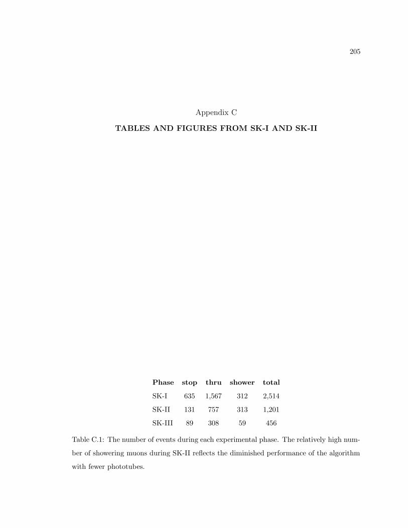
205
Appendix C
TABLES AND FIGURES FROM SK-I AND SK-II
Phase stop thru shower total
SK-I 635 1,567 312 2,514
SK-II 131 757 313 1,201
SK-III 89 308 59 456
Table C.1: The number of events during each experimental phase. The relatively high num-
ber of showering muons during SK-II reflects the diminished performance of the algorithm
with fewer phototubes.
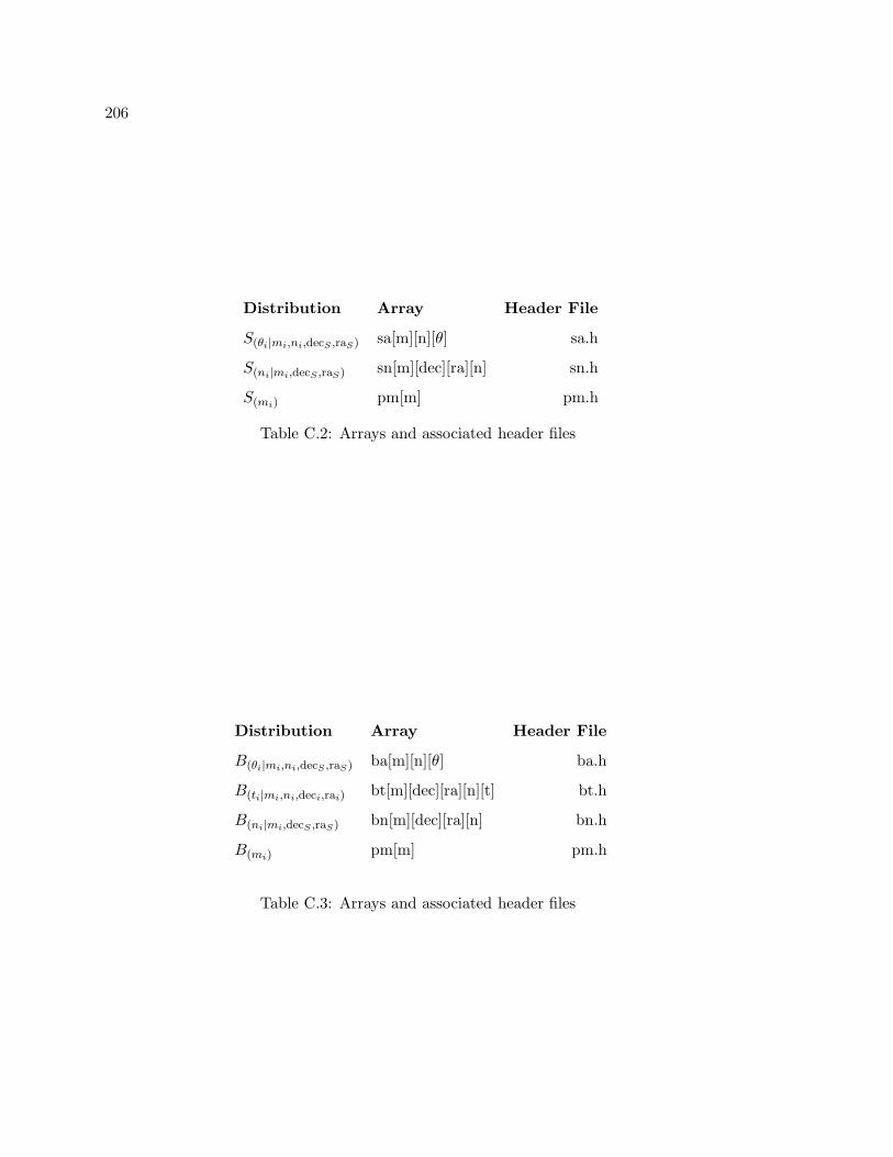
206
Distribution Array Header File
S(θi|mi,ni,decS ,raS) sa[m][n][θ] sa.h
S(ni|mi,decS ,raS) sn[m][dec][ra][n] sn.h
S(mi) pm[m] pm.h
Table C.2: Arrays and associated header files
Distribution Array Header File
B(θi|mi,ni,decS ,raS) ba[m][n][θ] ba.h
B(ti|mi,ni,deci,rai) bt[m][dec][ra][n][t] bt.h
B(ni|mi,decS ,raS) bn[m][dec][ra][n] bn.h
B(mi) pm[m] pm.h
Table C.3: Arrays and associated header files
207
VITA
Eric Thrane was born on May 13, 1981 to Michele and Gary Thrane. He grew up in
Arlington Heights, IL where he attended Buffalo Grove High School from 1995 to 1999.
He earned his BS from the University of Michigan where he graduated with highest honors
in 2003. His undergraduate thesis, Flat Electron Beam Dynamics: A Comparison of Data
with Simulation, was written under the supervision of Prof. David Gerdes. In 2003 he
began graduate school at the University of Washington as a Ken Young Fellow, working for
Prof. Jeff Wilkes on the Super-Kamiokande experiment. After obtaining his PhD, he will
move to the University of Minnesota to work with Professor Vuk Mandic as a postdoctoral
researcher on the LIGO experiment.