a scalable numerical method for simulating flows around high

Commun. Comput. Phys.doi: 10.4208/cicp.150313.070513s

Vol. x, No. x, pp. 1-15xxx 20xx

A Scalable Numerical Method for Simulating Flows

Around High-Speed Train Under Crosswind Conditions

Zhengzheng Yan1, Rongliang Chen1, Yubo Zhao1 and Xiao-Chuan Cai2,∗

1 Shenzhen Institutes of Advanced Technology, Chinese Academy of Sciences, Shenzhen518055, P.R. China.2 Department of Computer Science, University of Colorado Boulder, Boulder, CO 80309,USA.

Received 15 March 2013; Accepted (in revised version) 7 May 2013

Communicated by Peter Jimack

Available online xxx

Abstract. This paper presents a parallel Newton-Krylov-Schwarz method for the nu-merical simulation of unsteady flows at high Reynolds number around a high-speedtrain under crosswind. With a realistic train geometry, a realistic Reynolds number,and a realistic wind speed, this is a very challenging computational problem. Be-cause of the limited parallel scalability, commercial CFD software is not suitable forsupercomputers with a large number of processors. We develop a Newton-Krylov-Schwarz based fully implicit method, and the corresponding parallel software, for the3D unsteady incompressible Navier-Stokes equations discretized with a stabilized fi-nite element method on very fine unstructured meshes. We test the algorithm andsoftware for flows passing a train modeled after China’s high-speed train CRH380B,and we also compare our results with results obtained from commercial CFD software.Our algorithm shows very good parallel scalability on a supercomputer with over onethousand processors.

AMS subject classifications: 76D05, 76F65, 65M55, 65Y05

Key words: Three-dimensional unsteady incompressible flows, high-speed train, crosswind, fullNavier-Stokes equations, Newton-Krylov-Schwarz algorithm, parallel computing.

1 Introduction

In recent years, high-speed trains with characteristics of high-speed, high-efficiency andlow-energy consumption have been rapidly developed. When the wind is strong, trains

∗Corresponding author. Email addresses: [email protected] (Z. Yan), [email protected] (R. Chen),[email protected] (Y. Zhao), [email protected] (X.-C. Cai)

http://www.global-sci.com/ 1 c©20xx Global-Science Press

2 Z. Yan et al. / Commun. Comput. Phys., x (20xx), pp. 1-15

experience certain aerodynamic phenomena such as increased drag and lift, reduced sta-bility and raised level of acoustic noise. Unfortunately, the increase of speed often en-hances these negative effects, and some of which may result in accidents if they are notcontrolled correctly. Several train accidents caused by crosswind were reported in [6,22].Crosswind is one of the main threats that impact passenger’s comfort and/or vehicle’ssafety in high-speed train transportation. Therefore, it is both important and necessaryto carefully study the aerodynamic performance of trains under crosswind conditions.

Experimental techniques and commercial software based numerical simulations arethe two main tools in the train industry since analytical techniques are only applicablefor a few limited cases. Experimental investigations are usually expensive and subjectto the restrictions of design cycle, special boundary conditions and Reynolds numbers,and sometimes become not applicable or even impossible for high-speed trains. Numer-ical simulations are used more often and now become an important engineering tool,especially in the early design stages.

Historically, numerical simulations of crosswind around a train are inherited from asimple model, the Ahmed body [1], which includes most of the flow features in a real ve-hicle. Khier et al. [16] first use Reynolds averaged Navier-Stokes (RANS) equations com-bined with the k−ǫ turbulence model to study the flow structures around a simplifiedtrain under crosswind. In recent years, researchers have applied other techniques in solv-ing this problem numerically. The majority of these simulations are to apply some kind ofstatistical techniques to reduce the computational cost. RANS [9], large eddy simulation(LES) [10, 11] and detached eddy simulation (DES) [7, 17] are the three main approaches.All of these approaches can successfully obtain the flow structures relatively accurately.However, with the speed of trains increasing, certain design problems neglected at lowspeed are raised, more detailed computations are needed for the operational safety of ahigh-speed train. In this paper, we solve the full Navier-Stokes equations numericallywithout any further simplifications, on a very fine mesh of size 10−3m in order to capturethe subtle features and obtain sufficiently accurate solutions. Due to the limitation ofcomputer memory and processing speed, this method is usually considered as a researchtool rather than an engineering tool. In the past few years, the full Navier-Stokes equa-tions have been successfully used to the low Reynolds number cases, but high Reynoldsnumber flows implies a wide instantaneous range of scales, and high computing cost.Thanks to the recent development of large scale parallel computers with a large num-ber of processors, the computational capability is improved significantly. This makes itpossible to use full Navier-Stokes for engineering problems like the aerodynamics of ahigh-speed train. Correspondingly, the parallel scalability becomes an important indica-tor of a good numerical algorithm.

In this work, we present a scalable parallel Newton-Krylov-Schwarz (NKS) methodfor the full unsteady incompressible Navier-Stokes equations describing the flows aroundhigh-speed train under crosswind. Generally speaking, the NKS method is suitable forsolving large, sparse nonlinear systems and has been widely applied in various prob-lems [4, 5, 13, 14, 20]. In our algorithm, a fully implicit backward difference scheme is

Z. Yan et al. / Commun. Comput. Phys., x (20xx), pp. 1-15 3

adopted for the temporal discretization and a stabilized finite element method for thespatial discretization on an unstructured tetrahedral mesh. The nonlinear systems aresolved by using an inexact Newton method in which the Jacobian system is solved ap-proximately rather than exactly at each time step. In each Newton step, a Krylov sub-space method (GMRES) is used as a linear solver which is accelerated by an overlappingSchwarz preconditioner [19]. In addition, the pressure and velocity variables are not sep-arated but coupled at each mesh point in the process of finite element analysis. The aim ofthis operation is to make it possible to construct point-block incomplete LU factorizationwhich is more stable than the classical pointwise ILU.

We study our algorithm and software for a realistic train geometry with high Reynoldsnumber. We also compare our methods with the commercial CFD software package AN-SYS CFX. The numerical results show that our simulations provide more detailed infor-mation of the flow structures and our algorithm shows a good parallel scalability.

The paper is organized as follows. The high-speed train model and the computa-tional domain are presented in Section 2. The governing equations, the finite elementdiscretization and the Newton-Krylov-Schwarz algorithm are described in Section 3. InSection 4, some computational results are reported. The paper ends with some remarksin Section 5.

2 Physical models

In this section, we first describe the vehicle model and then discuss the computationaldomain and the gust model.

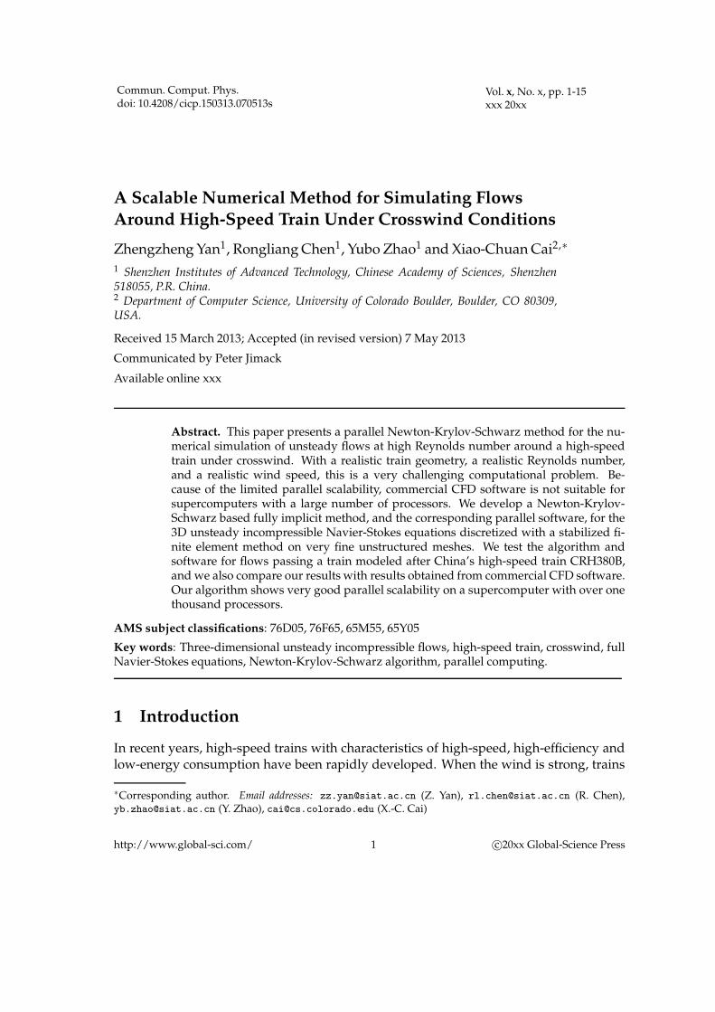
The train model is derived from China’s new generation of high-speed train shownin Fig. 1, namely CRH380B, which is designed for passenger transportation. The opera-tion speed is 300km/h and the maximum speed is up to 380km/h [21]. The geometry issymmetric and consists of four sets of wheels, a locomotive and a container. To simulatean actual train, we use the full scale parameters. The length of locomotive and containerare 24.75m and 24.01m, respectively, which make the total length of the model L=48.76m.The height of the platform from the ground is 0.915m. The width and height of the trainare W=3.26m and H=3.39m, respectively.

The computational domain for the high-speed train subject to crosswind is shown inFig. 1. This domain is chosen as in [16] and it is large enough to avoid the influence ofthe boundaries. The wind-inlet boundary (face ABFE) and the outflow boundary (faceDCGH ) are set to 10H and 13.3H far from the train, respectively. The distance betweenthe inlet boundary (face ABCD) and the nose of the train is 13.3H, the distance betweenthe outflow boundary (face FGHE) and the end of the train is 26.6H. The height of thecomputational domain (ground face BCGF to top face ADHE) is set to 10H.

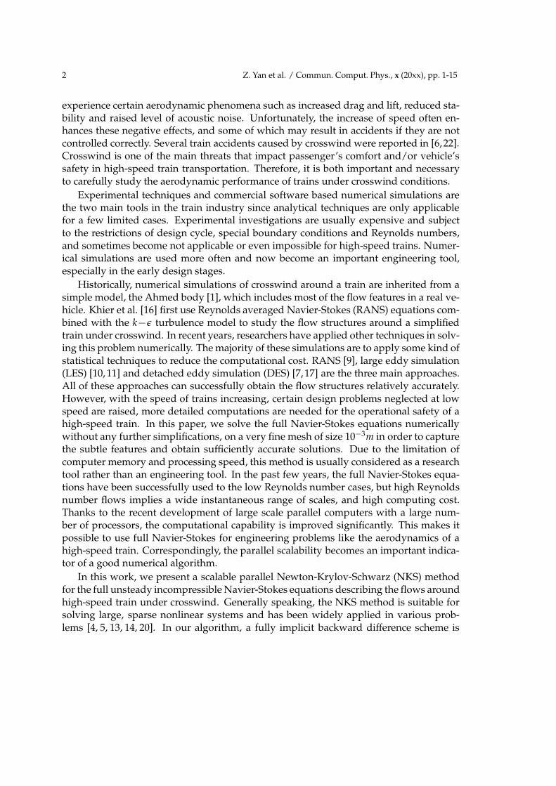
We assume that the direction of the crosswind is perpendicular to the direction thatthe train travels. The impact of the crosswind is the result of the velocity of the windand the train, so the effect of the crosswind can be strong even if the crosswind’s velocity


Figure 1: Dimensions of the model train and the computational domain.

Figure 2: Effective crosswind.

is low. The yaw angle describes the direction between the effective crosswind and thedirection at which the train travels, as Fig. 2 shows.

In practice, the wind velocity is stochastic and is usually influenced by the weathercondition and the topography of the nature environment, therefore in this particular ex-periment, we set a few functions that vary in both time and space to describe the veloci-ties of the wind and the train,

Vwind=−Vmaxwind

4(y−a)(y−b)

(b−a)2t, (2.1)

where a=−44m, b=136m are the minimum and maximum y values of the computationaldomain.

Vtrain=−Vmaxtrain

4(x−c)(x−d)

(d−c)2t, (2.2)

where c=−34.63m, d=45.63m are the minimum and maximum x values of the compu-tational domain. In our simulation, the flows around the train are initialized with zerovelocity and pressure everywhere.


3 Numerical methods

In this paper, the full 3D unsteady incompressible Navier-Stokes equations are used todescribe the flows in the spatial domain Ω⊂R3,

∇·u=0 in Ω, (3.1)

ρ

(

∂u

∂t+u·∇u

)

=−∇p+f+µ∇2u in Ω, (3.2)

where u is the velocity representing the three components in the Cartesian coordinates x,y and z. ρ, p and µ are the density, pressure, dynamic viscosity, respectively. f is the bodyforce. The governing equations (3.1) and (3.2) are equipped with boundary conditions on∂Ω=Γinlet∪Γoutlet∪Γwall

u=g on Γinlet, (3.3a)

u=0 on Γwall, (3.3b)

µ∂u

∂n−pn=0 on Γoutlet, (3.3c)

and the initial conditionu=u0 in Ω at t=0. (3.4)

Here g represents the effective crosswind velocity.To solve the set of governing equations, we first employ a P1-P1 stabilized finite el-

ement method introduced in [8] for the spatial discretization on the unstructured tetra-hedral mesh and an implicit backward Euler finite difference formula for the temporaldiscretization. Because of the page limit, we don’t discuss the details of the finite elementdiscretization in this paper. Then, the governing equations are turned into the followingsystem of nonlinear algebraic equations,

xn−xn−1

∆t=S(xn), (3.5)

where ∆t is the time step size and S(xn) represents the system after the spatial discretiza-tion without the temporal term at the nth time step. A large, sparse, nonlinear system

Fn(xn)=0, (3.6)

needs to be solved at each time step. In addition, when defining the unknowns vector xn

of nodal values, the pressure and the velocity variables, are not ordered field-by-field likemost approaches but element-by-element. The aim is to avoid the saddle point problemwhen solving the Jacobian system arising from the field-by-field ordering [12] because thesaddle point problem significantly affects the convergence and the parallel performance.

In this work, we solve the nonlinear system (3.6) by a Newton-Krylov-Schwarz (NKS)algorithm. Roughly speaking, the NKS algorithm consists of three components, a nonlin-ear solver, a linear solver at each Newton step and an accelerator. The basic steps of thealgorithm are listed below,


Step (a): Get an initial guess xn0 using the solution of previous time step xn−1,

xn0 =xn−1. (3.7)

Step (b): Obtain the Newton direction snk by solving the following preconditioned Jacobian system

inexactly with GMRES.

Jnk (Mn

k )−1Mn

k snk =−Fn(xn

k ), (3.8)

where Jnk is the Jacobian of Fn at xn

k , (Mnk )

−1 is an additive Schwarz preconditioner.

Step (c): Find a step length λnk using a cubic line search to update the approximation as follow,

xnk+1=xn

k +λnk sn

k , (3.9)

where xnk and xn

k+1 are the current and new approximation of xn, respectively.

In Step (b), we solve the Jacobian system (3.8) inexactly by satisfying the condition

‖F(xnk )+ Jn

k snk ‖≤ηk‖F(xn

k )‖, (3.10)

where ηk is the forcing term used to control the accuracy of the solution.

Without preconditioning, GMRES in Step (b) usually converges slowly or even doesn’tconverge. In our algorithm, an overlapping restricted additive Schwarz (RAS) method [3]is employed as the preconditioner to accelerate the convergence. We first partition thecomputational domain Ω into np non-overlapping subdomains Ωi, i=1,2,··· ,np where np

is the number of processors. Then we get the overlapping subdomains Ωδi by extending

δ layers of mesh elements from the adjacent subdomains. Then each overlapping sub-domain Ωδ

i has its local Jacobian matrix Ji and the global-to-local restriction operator Rδi

is defined to return all of the degree of freedom (DOF) belonging to Ωδi from the global

vector of unknowns. We define R0i as the restriction operator for the non-overlapping

subdomain Ωi similar as Rδi . Then, the RAS preconditioner is defined as

MRAS=np

∑i=1

(R0i )

TB−1i Rδ

i , (3.11)

where B−1i is the local preconditioner. In this paper, The linear system corresponding to

B−1i is solved by a point-block incomplete LU [18] with some levels of fill-in, which is

more economical than LU as the local preconditioner.

4 Numerical experiments and discussions

In this section, a test case with Vwind = 20m/s and Vtrain = 100m/s is studied. The fluidmaterial we adopt is air at 25C with density ρ=1.185kg/m3 and dynamic viscosity µ=


1.831×10−5kg/ms. The yaw angle β≈20.27 and the Reynolds number Re=2.238×107

is defined as

Re=ρu∞D

µ, (4.1)

where u∞ is the freestream velocity which equals to the effective crosswind velocity, D isthe characteristic length of the train and D=H=3.39m.

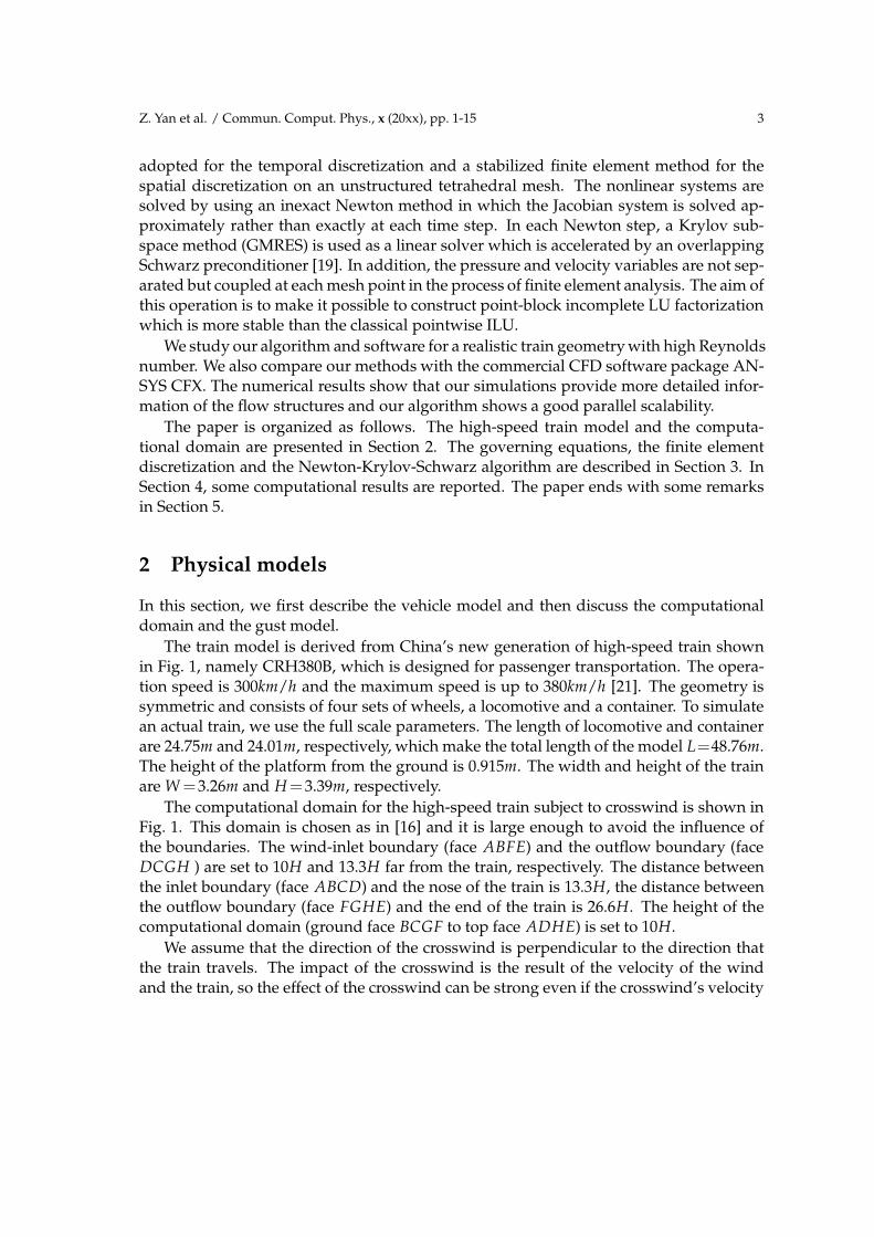
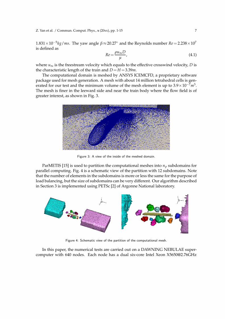
The computational domain is meshed by ANSYS ICEMCFD, a proprietary softwarepackage used for mesh generation. A mesh with about 14 million tetrahedral cells is gen-erated for our test and the minimum volume of the mesh element is up to 3.9×10−7m3.The mesh is finer in the leeward side and near the train body where the flow field is ofgreater interest, as shown in Fig. 3.

Figure 3: A view of the inside of the meshed domain.

ParMETIS [15] is used to partition the computational meshes into np subdomains forparallel computing. Fig. 4 is a schematic view of the partition with 12 subdomains. Notethat the number of elements in the subdomains is more or less the same for the purpose ofload balancing, but the size of subdomains can be very different. Our algorithm describedin Section 3 is implemented using PETSc [2] of Argonne National laboratory.

Figure 4: Schematic view of the partition of the computational mesh.

In this paper, the numerical tests are carried out on a DAWNING NEBULAE super-computer with 640 nodes. Each node has a dual six-core Intel Xeon [email protected]


processor and 24GB of memory. The numerical results obtained by our algorithm andANSYS CFX are used for comparative analysis at first. Then, the parallel performance ofour algorithm is investigated for solving these large-scale computational problems.

4.1 Comparative assessment of numerical results obtained by our algorithmand ANSYS CFX

We compare the NKS method and RANS with k−ǫ closure model by ANSYS CFX. Thesame geometry, computational mesh and boundary conditions are applied for these twosimulations. Using an element-based finite volume approach, CFX applies the standardk−ǫ model to describe the turbulence behavior. A second-order backward Euler schemeis used for the transient term. The residual target of root mean square (RMS) conver-gence criteria is set to 1.0×10−6. In the NKS algorithm, the computational domain isdivided into subdomains and the number of subdomains is equal to the number of pro-cessors. The relative tolerances of linear and nonlinear convergence are set to 1.0×10−4

and 1.0×10−6, respectively. For these two simulations, a constant time step ∆t is set to4.0×10−3s throughout the entire simulation, the solutions obtained at t=1s are used forthe comparison.

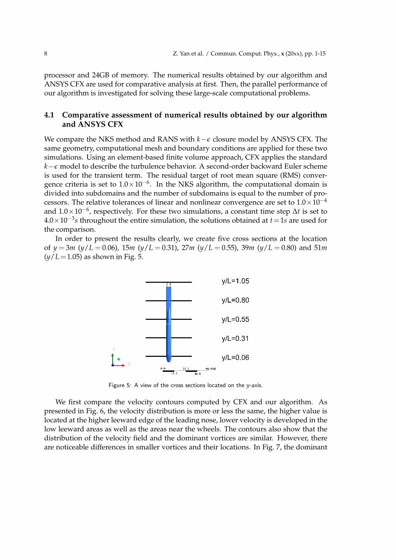
In order to present the results clearly, we create five cross sections at the locationof y = 3m (y/L = 0.06), 15m (y/L = 0.31), 27m (y/L = 0.55), 39m (y/L = 0.80) and 51m(y/L=1.05) as shown in Fig. 5.

Figure 5: A view of the cross sections located on the y-axis.

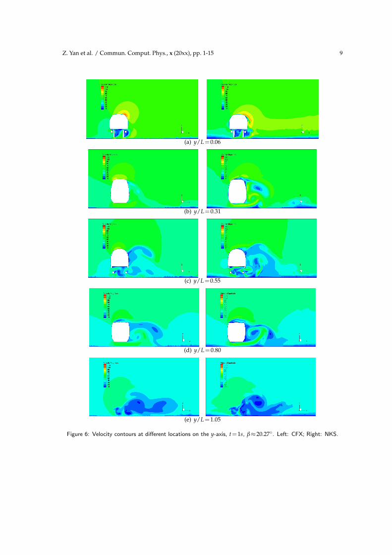
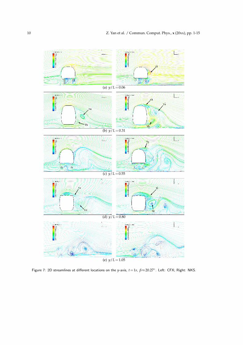
We first compare the velocity contours computed by CFX and our algorithm. Aspresented in Fig. 6, the velocity distribution is more or less the same, the higher value islocated at the higher leeward edge of the leading nose, lower velocity is developed in thelow leeward areas as well as the areas near the wheels. The contours also show that thedistribution of the velocity field and the dominant vortices are similar. However, thereare noticeable differences in smaller vortices and their locations. In Fig. 7, the dominant


(a) y/L=0.06

(b) y/L=0.31

(c) y/L=0.55

(d) y/L=0.80

(e) y/L=1.05

Figure 6: Velocity contours at different locations on the y-axis, t=1s, β≈20.27. Left: CFX; Right: NKS.


(a) y/L=0.06

(b) y/L=0.31

(c) y/L=0.55

(d) y/L=0.80

(e) y/L=1.05

Figure 7: 2D streamlines at different locations on the y-axis, t=1s, β≈20.27 . Left: CFX; Right: NKS.


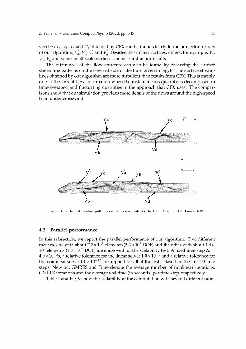
vortices Va, Vb, Vc and Vd obtained by CFX can be found clearly in the numerical resultsof our algorithm, V

′

a, V′

b, V′

c and V′

d. Besides these main vortices, others, for example, V′

e ,

V′

f , V′

g and some small-scale vortices can be found in our results.

The differences of the flow structure can also be found by observing the surfacestreamline patterns on the leeward side of the train given in Fig. 8. The surface stream-lines obtained by our algorithm are more turbulent than results from CFX. This is mainlydue to the loss of flow information when the instantaneous quantity is decomposed intime-averaged and fluctuating quantities in the approach that CFX uses. The compar-isons show that our simulation provides more details of the flows around the high-speedtrain under crosswind.

Figure 8: Surface streamline patterns on the leeward side for the train. Upper: CFX; Lower: NKS.

4.2 Parallel performance

In this subsection, we report the parallel performance of our algorithm. Two differentmeshes, one with about 7.2×106 elements (5.3×106 DOF) and the other with about 1.4×107 elements (1.0×107 DOF) are employed for the scalability test. A fixed time step ∆t=4.0×10−3s, a relative tolerance for the linear solver 1.0×10−4 and a relative tolerance forthe nonlinear solver 1.0×10−12 are applied for all of the tests. Based on the first 20 timesteps, Newton, GMRES and Time denote the average number of nonlinear iterations,GMRES iterations and the average walltime (in seconds) per time step, respectively.

Table 1 and Fig. 9 show the scalability of the computation with several different num-


Table 1: Parallel performance of the NKS algorithm. Here the level of ILU fill-ins ℓ=1, the overlapping size forRAS δ=4.

npDOF=5.3×106 DOF=1.0×107

Newton GMRES Time Newton GMRES Time

128 3.691 94.039 137.915 - - -

256 3.691 92.263 74.811 3.762 122.949 171.827

512 3.762 94.797 46.722 3.524 120.743 93.644

1024 3.143 87.182 32.701 3.619 123.092 62.427

128 256 512 102432.701

46.772

62.427

74.811

93.644

137.915

171.827

Number of processors

Co

mp

ute

tim

e

DOF=5.3 × 106

DOF=1.0 × 107

128 256 512 10241

2

4

8

Number of processors

Sp

eed

up

DOF=5.3 × 106

DOF=1.0 × 107

Ideal

Figure 9: The average compute time per time step and the speedup (log-log scaled). Here the level of ILUfill-ins ℓ=1, the overlapping size for RAS δ=4.

ber of processors. We see that the number of nonlinear iterations per time step is quitesmall since the solution of the previous time step is used as the initial guess. The parallelresults including the number of linear iterations and the total compute time show thatour algorithm and software implementation are quite scalable.

In subdomain solvers, the level of fill-ins of ILU affects the performance of the NKSalgorithm. Tables 2 and 3 show the comparison with different level of fill-ins ℓ. We seethat larger ℓ helps in reducing the number of GMRES iterations but fewer level of ILUfill-ins ℓ=1 provides better compute time.

We next present a comparison of additive Schwarz method with overlap δ changingfrom 0 to 4 using 1024 cores. Generally speaking, in the additive Schwarz method, themore overlap between subdomains, the faster the convergence is. However, the sub-problems as well as the amount of communication become larger at the same time andresult in the computing time increase. So, finding a good trade-off between the numberof iterations and the computing time is important. The results shown in Table 4 verifythis view. From this table, we observe that the number of GMRES iterations is decreasedwhen large overlaps are used, but smaller overlap, δ=2, offers the best timing results.


Table 2: Performance of NKS with respect to the level of ILU fill-ins ℓ. Here the overlapping size for RAS δ=4,DOF=5.3×106.

npNewton GMRES Time

ILU(0) ILU(1) ILU(2) ILU(0) ILU(1) ILU(2) ILU(0) ILU(1) ILU(2)

128 3.810 3.691 3.476 172.750 94.039 57.233 151.039 137.915 170.280

256 3.857 3.619 3.190 168.605 92.263 55.015 84.147 74.811 82.465

512 3.875 3.762 3.286 166.988 94.797 57.203 52.792 46.772 50.091

1024 3.714 3.143 3.667 167.885 87.182 61.169 45.439 32.701 40.292

Table 3: Performance of NKS with respect to the level of ILU fill-ins ℓ. Here the overlapping size for RAS δ=4,DOF=1.0×107.

npNewton GMRES Time

ILU(0) ILU(1) ILU(2) ILU(0) ILU(1) ILU(2) ILU(0) ILU(1) ILU(2)

256 3.810 3.762 3.714 254.600 122.949 84.603 373.825 171.827 223.134

512 3.810 3.524 3.810 250.512 120.743 86.838 366.144 93.644 124.798

1024 3.762 3.619 3.492 256.937 123.092 84.569 149.742 62.427 80.702

Table 4: Performance of NKS with respect to the overlapping size δ. Here the level of ILU fill-ins ℓ=2.

RAS overlap δDOF=5.3×106 DOF=1.0×107

Newton GMRES Time Newton GMRES Time

0 3.810 113.950 67.721 3.810 148.600 120.346

1 3.810 81.975 39.643 3.810 114.550 93.001

2 3.476 66.740 34.336 3.714 99.346 77.354

3 3.667 64.649 39.588 3.667 93.104 78.375

4 3.667 61.169 40.292 3.429 84.569 80.702

4.3 Influence of Reynolds number

When solving fluid dynamic problems like the external flows around the high-speed trainunder crosswind, the Reynolds number has a major impact on the complexity of the flowsand the difficulty of the discrete system of equations. In this test, we consider Reynolds

Table 5: The robustness of the algorithm with respect to various values of Reynolds numbers. Here DOF=1.0×107, np=1024.

Wind velocity Train velocity Reynolds number Newton GMRES Time

0 1 2.194×105 2.857 78.517 65.100

0 5 1.097×106 2.857 78.233 70.583

0 10 2.194×106 2.905 78.672 61.992

10 20 4.906×106 2.905 78.656 70.277

30 100 2.291×107 3.476 85.616 82.522


numbers from 2.194×105 to 2.291×107 depending on the velocity of the crosswind andthe speed of the train. The numerical results shown in Table 5 indicate the NKS algorithmworks well for this range of Reynolds number.

5 Conclusions

Accurate simulation of external flows around a high-speed train under crosswind is achallenging computational problem. Finding a robust and scalable algorithm is a keyissue for obtaining meaningful results in a timely matter for actual engineering applica-tions. In this paper, we developed a parallel Newton-Krylov-Schwarz algorithm for thefully implicit solution of the full 3D unsteady incompressible Navier-Stokes equations.After the discretization, the nonlinear algebraic systems are solved by using an inex-act Newton method in each time step. The GMRES method accelerated by an overlap-ping Schwarz preconditioner is used as the linear solver in each Newton step. We testedthe algorithm for flows passing a high-speed train with realistic geometry and differentReynolds numbers. Based on the numerical results, we concluded that the algorithm andour software implementation are robust with a wide range of Reynolds numbers up to2.291×107 and exhibit a good scalability with up to 1024 processors.

Acknowledgments

The research is supported in part by the Knowledge Innovation Program of the ChineseAcademy of Sciences under KJCX2-EW-L01, and the International Cooperation Project ofGuangdong province under 2011B050400037.

References

[1] S. R. Ahmed, G. Ramm, and G. Faltin, Some salient features of the time-averaged groundvehicle wake, SAE paper, 840300, 1984.

[2] S. Balay, K. Buschelman, W. D. Gropp, D. Kaushik, M. Knepley, L. C. McInnes, B. F. Smith,and, H. Zhang, PETSc Users Manual, Technical Report, Argonne National Laboratory, 2012.

[3] X.-C. Cai and M. Sarkis, A restricted additive Schwarz preconditioner for general sparselinear systems, SIAM J. Sci. Comput., 21 (1999), 792-797.

[4] R. Chen and X.-C. Cai, Parallel one-shot Lagrange-Newton-Krylov-Schwarz algorithms forshape optimization of steady incompressible flows, SIAM J. Sci. Comput., 34 (2012), 584-605.

[5] R. Chen, Y. Wu, Z. Yan, Y. Zhao, and X.-C. Cai, A parallel domain decomposition method for3D unsteady incompressible flows at high Reynolds number, J. Sci. Comput., (to appear).

[6] B. Diedrichs, Studies of Two Aerodynamic Effects on High-Speed Trains: Crosswind Stabil-ity and Discomforting Car Body Vibrations Inside Tunnels, Ph.D. Thesis, Royal Institute ofTechnology (KTH), 2006.

[7] T. Favre, B. Diedrichs, and G. Efraimsson, Detached-Eddy simulations applied to unsteadycrosswind aerodynamics of ground vehicles, Progress in Hybrid RANS-LES Modelling,Springer, 2010, 167-177.


[8] L. P. Franca and S. L. Frey, Stabilized finite element method: II. The incompressible Navier-Stokes equations, Comput. Methods Appl. Mech. Engrg., 99 (1992), 209-233.

[9] E. Guilmineau, Computational study of flow around a simplified car body, J. Wind. Eng.Ind. Aerod., 96 (2008), 1207-1217.

[10] H. Hemida and C. Baker, Large-eddy simulation of the flow around a freight wagon sub-jected to a crosswind, Comput. Fluids, 39 (2010), 1944-1956.

[11] H. Hemida and S. Krajnovic, LES study of the impact of the wake structures on the aerody-namics of a simplified ICE2 train subjected to a side wind, presented at the 4th InternationalConference on Computational Fluid Dynamics, Ghent, Belgium, July 10-14, 2006.

[12] Q. Hu and J. Zou, Nonlinear inexact Uzawa algorithms for linear and nonlinear saddle-pointproblems, SIAM J. Optim., 16 (2006), 798-825.

[13] F.-N. Hwang and X.-C. Cai, A parallel nonlinear additive Schwarz preconditioned inexactNewton algorithm for incompressible Navier-Stokes equations, J. Comput. Phys., 204 (2005),666-691.

[14] F.-N. Hwang, C.-Y. Wu, and X.-C. Cai, Numerical simulation of three-dimensional bloodflows using domain decomposition method on parallel computer, J. CSME., 31 (2010), 199-208.

[15] G. Karypis, R. Aggarwal, K. Schloegel, V. Kumar, and S. Shekhar, ParMETIS home page,http://glaros.dtc.umn.edu/gkhome/metis/parmetis/overview.

[16] W. Khier, M. Breuer, and F. Durst, Flow structure around trains under side wind conditions:a numerical study, Comput. Fluids, 29 (2000), 179-195.

[17] S. Krajnovic, Numerical simulation of the flow around an ICE2 train under the influence of awind gust, presented at the International Conference on Railway Engineering, Hong Kong,China, March 25-28, 2008.

[18] Y. Saad, Iterative Method for Sparse Linear Systems, SIAM, 2003.[19] B. F. Smith, P. E. Bjørstad, and W. D. Gropp, Domain Decomposition Parallel Multilevel

Methods for Elliptic Partial Differential Equations, Cambridge university press, Cambridge,1996.

[20] Y. Wu and X.-C. Cai, A parallel two-level method for simulating blood flows in branchingarteries with the resistive boundary condition, Comput. Fluids, 45 (2011), 92-102.

[21] G. W. Yang, D. L. Guo, S. B. Yao, and C. H. Liu, Aerodynamic design for China new high-speed trains, Sci. China Tech. Sci., 55 (2012), 1923-1928.

[22] D. Zhou, H. Q. Tian, and Z. J. Lu, Influence of the strong crosswind on aerodynamic perfor-mance of passenger train running on embankment, J. Traffic Transp. Eng., 7 (2007), 6-9.

a scalable numerical method for simulating flows around high

Documents