A Render Model For Particle System

Hanxin Jia

A Thesis

in

The Department

of

Engineering and Computer Science

Presented in Partial Fulfillment of the Requirements

for the Degree of

Master of Computer Science at

Concordia University

Montreal, Quebec, Canada

January 2016

c© Hanxin Jia, 2016

CONCORDIA UNIVERSITY

School of Graduate Studies

This is to certify that the thesis prepared

By: Hanxin Jia

Entitled: A Render Model For Particle System

and submitted in partial fulfillment of the requirements for the degree of

Master of Computer Science

complies with the regulations of this University and meets the accepted standards with respect to

originality and quality.

Signed by the Final Examining Committee:

ChairDr. E. Shihab

ExaminerDr. T. Fevens

SupervisorDr. Sudhir P. Mudur

Co-supervisorDr. Tiberiu Popa

Approved byChair of Department of Engineering and Computer Science

2016Dean of Faculty of Engineering and Computer Science

Abstract

A Render Model For Particle System

Hanxin Jia

Particle system is a very commonly used system in computer graphics. It can be used to simulate

many objects in the real world, such as liquid simulation, smoke simulation and so on. Now, a

new method called welding simulation has been developed. In this simulation, it needs to give the

particle system a metal-like surface. Therefore, in this thesis, we developed a render model which

can make a particle system have a metal-like surface. This render model can be used in welding

simulation application and also for other applications based on particle systems with metal-like

surface.

iii

Acknowledgments

First and foremost, I would like to show my deepest gratitude to my supervisor, Dr. Tiberiu Popa and

Dr. Sudhir P. Mudur. They are respectable, responsible and resourceful scholars, who has provided

me with valuable guidance in every stage of the writing of this thesis. Without their excellent

instruction, impressive professionalism and patience, I could not have completed my thesis.

I shall extend my thanks to my group member Gu Qing for all his kind help. My sincere appreciation

also goes to all my teachers at Concordia University who have helped me to develop the fundamental

and essential academic competence.

Last but not the least, I would like to thank all my friends and also my parents for their encourage-

ment and support.

iv

Contents

List of Figures viii

1 Introduction 1

1.1 Smoothed particle hydrodynamics . . . . . . . . . . . . . . . . . . . . . . . . . . 2

1.2 Render Model . . . . . . . . . . . . . . . . . . . . . . . . . . . . . . . . . . . . . 3

2 Background 5

2.1 SPH surface reconstruction method . . . . . . . . . . . . . . . . . . . . . . . . . . 5

2.1.1 Marching Cube . . . . . . . . . . . . . . . . . . . . . . . . . . . . . . . . 5

2.1.2 point-based surface visualization . . . . . . . . . . . . . . . . . . . . . . . 7

2.1.3 Image-Space 3D Metaballs . . . . . . . . . . . . . . . . . . . . . . . . . . 8

2.1.4 Volume Ray Casting . . . . . . . . . . . . . . . . . . . . . . . . . . . . . 11

2.1.5 Screen Space Rendering . . . . . . . . . . . . . . . . . . . . . . . . . . . 15

2.2 Rendering of Metal Materials . . . . . . . . . . . . . . . . . . . . . . . . . . . . . 16

2.2.1 Texture for Model . . . . . . . . . . . . . . . . . . . . . . . . . . . . . . 16

2.2.2 Reflectance Models . . . . . . . . . . . . . . . . . . . . . . . . . . . . . . 18

v

2.2.3 BSSRDF and BRDF . . . . . . . . . . . . . . . . . . . . . . . . . . . . . 22

2.2.4 Fresnel Term and Surface Reflectance . . . . . . . . . . . . . . . . . . . . 25

2.2.5 Isotropic and Anisotropicls Surfaces . . . . . . . . . . . . . . . . . . . . . 27

3 Screen Space Rendering Method 28

3.1 Generate Depth Image . . . . . . . . . . . . . . . . . . . . . . . . . . . . . . . . 28

3.2 Calculate Normal . . . . . . . . . . . . . . . . . . . . . . . . . . . . . . . . . . . 30

3.2.1 Reconstruction Position From Depth . . . . . . . . . . . . . . . . . . . . . 30

3.2.2 Calculate Normal . . . . . . . . . . . . . . . . . . . . . . . . . . . . . . . 31

3.3 Smooth Depth Image . . . . . . . . . . . . . . . . . . . . . . . . . . . . . . . . . 33

3.3.1 Gaussian Blur . . . . . . . . . . . . . . . . . . . . . . . . . . . . . . . . . 33

3.3.2 Bilateral Blur . . . . . . . . . . . . . . . . . . . . . . . . . . . . . . . . . 34

3.3.3 Adaptive Kernel Size . . . . . . . . . . . . . . . . . . . . . . . . . . . . . 37

3.3.4 Adaptive Particle Ratio . . . . . . . . . . . . . . . . . . . . . . . . . . . . 37

4 Physically Based Rendering 41

4.1 Rendering Equation . . . . . . . . . . . . . . . . . . . . . . . . . . . . . . . . . . 41

4.2 Light in PBR . . . . . . . . . . . . . . . . . . . . . . . . . . . . . . . . . . . . . 44

4.2.1 Direct Light . . . . . . . . . . . . . . . . . . . . . . . . . . . . . . . . . . 44

4.2.2 Indirect Light . . . . . . . . . . . . . . . . . . . . . . . . . . . . . . . . . 48

4.3 Final Lighting Calculate . . . . . . . . . . . . . . . . . . . . . . . . . . . . . . . 55

vi

5 Conclusion and Discuss 57

5.1 Future Work . . . . . . . . . . . . . . . . . . . . . . . . . . . . . . . . . . . . . . 58

Bibliography 60

vii

List of Figures

Figure 1.1 The pipeline of our render model. . . . . . . . . . . . . . . . . . . . . . . . 4

Figure 2.1 a cube with index . . . . . . . . . . . . . . . . . . . . . . . . . . . . . . . 6

Figure 2.2 all uniqu intersection cases . . . . . . . . . . . . . . . . . . . . . . . . . . 6

Figure 2.3 The overview of the point-based surface visulaization . . . . . . . . . . . . 8

Figure 2.4 The processes of the walking depth plane, dashed lines represent access to

the frame buffer objects, and the solid lines represent the control flow . . . . . . . 11

Figure 2.5 basic framework for rendering metaballs . . . . . . . . . . . . . . . . . . . 13

Figure 2.6 The process of maintaining a list based on the viewing ray in Figure 2.4 . . 13

Figure 2.7 metaballs with dash lines are hidden by the metaballs front . . . . . . . . . 14

Figure 2.8 a perspective grid . . . . . . . . . . . . . . . . . . . . . . . . . . . . . . . 16

Figure 2.9 add a texture to a 3D model . . . . . . . . . . . . . . . . . . . . . . . . . . 17

Figure 2.10 sphere add a bump map appears to have more surface details . . . . . . . . 17

Figure 2.11 add normal map to an object . . . . . . . . . . . . . . . . . . . . . . . . . 18

Figure 2.12 Perfect diffuse, perfect specular and glossy specular . . . . . . . . . . . . . 20

Figure 2.13 direction vectors using in Phong model and Blinn-Phong model . . . . . . . 21

viii

Figure 2.14 some of the reflected light could be blocked by nearby micro-facets and some

of the light from light source could also be blocked by micro-facets nearby . . . . . 22

Figure 2.15 a. a bidirectional reflection distribution function(BRDF) - light incomes and

outcomes at the same position. B. a bidirectional surface scattering reflectance dis-

tribution function(BSSRDF) the light incomes and outcomes at different places. C.

A Cook-Torrance reflectance model which treats a surface as a set of many micro-

facets, each facets has its own normal n. . . . . . . . . . . . . . . . . . . . . . . . 23

Figure 2.16 In colored metals such as silver, aluminum, gold specular reflection changes

their color based on thier properties. In this image, the metal bowl has a silver-gray

colored highlight . . . . . . . . . . . . . . . . . . . . . . . . . . . . . . . . . . . 24

Figure 2.17 reflected law and Snell’s law . . . . . . . . . . . . . . . . . . . . . . . . . 25

Figure 2.18 showing the difference between dielectrics and metals. For dielectric mate-

rials on surfaces have relatively low reflectance level of 20% or less for most of the

angular range, while metals have a pretty high level of reflectance of 60% and above

(Westin and Torrance. (n.d.)) . . . . . . . . . . . . . . . . . . . . . . . . . . . . . 27

Figure 3.1 The viewer can only see a subset of the particles. Also, they can almost never

see the opposing surface. These factors motivate the need for creating the surface in

user’s perspective only and particles outside the viewer’s perspective are clipped. . 29

Figure 3.2 turn the particles in Figure 2.1 into point sprites, the point always face the

viewer . . . . . . . . . . . . . . . . . . . . . . . . . . . . . . . . . . . . . . . . . 29

Figure 3.3 Point sprites which are ”below” the surface will not be rendered. . . . . . . 29

Figure 3.4 After changing depth, the point sprites are turned into hemispheres. . . . . . 30

Figure 3.5 This figure shows the result of depth image . . . . . . . . . . . . . . . . . . 31

Figure 3.6 the normal is the cross product between ddx and ddy . . . . . . . . . . . . . 32

ix

Figure 3.7 The normal image calculated through depth image . . . . . . . . . . . . . . 32

Figure 3.8 Gaussian Function . . . . . . . . . . . . . . . . . . . . . . . . . . . . . . . 33

Figure 3.9 blue quad is the position of center pixel, middle figure is the shape of Gaus-

sian blur, right is the shape of Bilateral blur . . . . . . . . . . . . . . . . . . . . . 35

Figure 3.10 A shows the normal image calculated through the depth image smoothed

by Gaussian Blur. B shows the normal image calculated through the depth image

smoothed by Bilateral Blur. We can find out that the edges of the object in the image

smoothed by Gaussian Blur have more noise than one smoothed by Bilateral Bulr . 36

Figure 3.11 A shows the result with adaptive ratio, B shows the result without adaptive

ratio . . . . . . . . . . . . . . . . . . . . . . . . . . . . . . . . . . . . . . . . . . 40

Figure 4.1 The rendering equation is used to describe the light emitted from a position

x along a particular viewing direction, using a BRDF and incoming light. . . . . . 43

Figure 4.2 a bunny rendered with direct diffuse light . . . . . . . . . . . . . . . . . . . 45

Figure 4.3 a bunny rendered with direct light . . . . . . . . . . . . . . . . . . . . . . . 47

Figure 4.4 known view ray and normal we can calculate reflect ray . . . . . . . . . . . 48

Figure 4.5 orange area represent the light rays coming from the environment to the

shaded pixel. . . . . . . . . . . . . . . . . . . . . . . . . . . . . . . . . . . . . . 49

Figure 4.6 a bunny rendered with diffuse light calculated through Spherical Harmonics 52

Figure 4.7 take a few samples and combine them together . . . . . . . . . . . . . . . . 53

Figure 4.8 25 Hammersley points in a unit square . . . . . . . . . . . . . . . . . . . . 54

Figure 4.9 take samples from environment based on the Hammersley Vector . . . . . . 55

Figure 4.10 This picture shows the result of indirect light . . . . . . . . . . . . . . . . . 56

Figure 5.1 a liquid metal with background reflectance . . . . . . . . . . . . . . . . . . 57

x

Figure 5.2 A shows a bunny constructed by particles. B shows a melting process with

that bunny . . . . . . . . . . . . . . . . . . . . . . . . . . . . . . . . . . . . . . . 58

Figure 5.3 two metal bars are wielded together. . . . . . . . . . . . . . . . . . . . . . 58

Figure 5.4 particle bunny with different roughness, a roughness = 0.1, b roughness =

0.5, c roughness = 0.9 . . . . . . . . . . . . . . . . . . . . . . . . . . . . . . . . . 59

xi

Chapter 1

Introduction

Physical simulation is a very popular filed of computer graphics, because it can be widely used in

many applications, such as video games, movies and so on. In this thesis, we focus on developing a

render model for fluid simulation which is a very popular topic in physical simulation. Presenting

fluid with particles is a good way to simulate fluid. Smoothed Particle Hydrodynamics (SPH) is

a commonly used method using particles to simulate fluid. It not only can be utilized in fluid

simulation but also in other applications, such as welding simulation. Welding simulation can be

utilized to train workers without costing lots of materials, which makes it very cost-effective in

industrial training. In order to simulate the welding, we need to make the particles have metal-like

surface. Nevertheless, most render model for SPH is used to give particles water-like performance.

Thus, in this thesis, we developed a render model which is used to give a particle system ,like SPH

,a metal-like surface. The render model in this thesis can be utilized to a particle system which

simulates the features of metal, for example, the wilding process simulation, metal compression or

transformation. In this thesis, we combine two techniques to achieve our goal. The first one is screen

space rendering introduced in 2009 (Wladimir J. van der Laan (2009a)) which is used to transform

the particle system to an entire model with a normal and smoothed surface. Based on the original

method, we add an adaptive particle size to make the result better. More details will be discussed in

Chapter 3. The second one is called physical based rendering. This technique can produce a metal

surface with variable roughness. This part will be discussed in Chapter 4. After combining these

1

two techniques, we developed a render model that can give a particle system a metal-like surface.

In the next section, we will give a brief introduction to SPH which is our original target system.

1.1 Smoothed particle hydrodynamics

Smoothed particle hydrodynamics (SPH) is a method using a particle system to simulate fluid flow.

This method is first introduced by Gingold and Monaghan in 1977 (Gingold and Monaghan (n.d.)).

In this method they use particles to represent water, and then use Navier-Stokes equations to calcu-

late velocity and then compute the position. The Navier-Stokes equation is:

∂u

∂t︸︷︷︸acceleration

= −1

ρ� p︸ ︷︷ ︸

presure

+ μ�2 u︸ ︷︷ ︸viscosity

+g (1)

In order to have a smoothed and continuous field, they need kernel function w to calculate this

equation:

Ai =∑j

mj

ρjAjW (xi − xj , h) (2)

A is the quantity that needs to be calculated, and Ai is the ith quantity. And j means the whole

neighbor particles around particle i, with the range of kernel size h. w is the smoothing kernel

function. Thus, when we compute the density we change A to density ρ. For viscosity we use

the differences between velocity to calculate. Viscosity is a very important quantity which is used

to stabilize the particle system and it only depends on velocity differences but not on absolute

velocities. The equation for calculating the force of viscosity is:

fviscosityi =

∑j

mj

ρj(uj − ui)�2 W (xi − xj , h) (3)

2

The pressure of each particle is calculated by the density. The equation for calculating pressure is:

pi = k(ρi − ρ0) (4)

Where ρ0 is the rest density of fluid which is the physical density of the fluid, for example, 1000kg/m3

for waters. In order to make the pressures symmetric, a bit change in the original equation is per-

formed:

fpressurei = −

∑j

mj

ρj

pi + pj2

ΔW (xi − xj , h) (5)

1.2 Render Model

Our render model is originally developed for SPH system, however, it can be actually used to other

particle systems which need metal-like rendering. The only problem is that some features in our

render model cannot be used without SPH system. For example, the adaptive particle size cannot be

implemented without color field which is required in SPH system. Our render model can be divided

into two parts, the first one is transforming particles into a model. In this part, we need a method

based on screen space rendering. Generally, Screen Space Rendering has 4 steps. First, we have an

obligation to generate a depth image of particles, in which we will render each particle as spherical

point sprites. In order to achieve a better result, we add an adaptive particle ratio to the original

method. Second, smooth depth image. This is a major step for screen space rendering. It contributes

the most to the final result. Through choosing different blur method, we will have multiple results.

In this paper, we mainly discuss Gaussian blur and bilateral blur. Third, calculate surface normals

and position from depth image which are smoothed in the previous step. The second part is utilized

to make the model transform particles to a metal-like surface. We use two kinds of light to render

it. The first one is direct light which is used to give the model base color and performance. We

mainly use Cook-Torrance BDRF to achieve the goal. The other one is indirect light which is used

for background reflection, including diffuse environment reflection and specular reflection. For the

diffuse environment reflection we use spherical harmonics lighting. And for the specular reflection,

3

we use importance sample to make the surface has specular reflection with unusual roughness level.

With these two kinds of light, we can create a metal-like surface with different roughness level.

Figure 1.1 shows the whole pipeline of our render model.

Figure 1.1: The pipeline of our render model.

4

Chapter 2

Background

2.1 SPH surface reconstruction method

2.1.1 Marching Cube

Marching cube is a classical render method, which was introduced by William E. Lorensen and

Harvey E. Cline in 1986 (William E. Lorensen (n.d.)). There are two mainly steps for reconstructing

isosurface. First, finding intersections between the edges of a cube and the volume. And then,

creating triangles based on the result from previous step.

As showed in Figure 2.1, given a cube which including 8 vertices (v0, v1, v2, ..., v7), and 12 edges

(e0, e1, e2, ..., e7). The isosurface is defined by an arbitrary value called iso-value, like a threshold,

which is usually calculated based on the specify requirement. The isosurface is generated depending

on the compare result between the vertices value in the cube and the iso-value, it will decide weather

the vertex is inside the surface or outside, or directly on the isosurface . All vertices in the cube are

compared with the iso-value. Each comparison will update a bit in the cube index which has total

8-bit. And then searching a look up index table which indexed by the cube index for an address in

an edge table which contains triangle edge connectivity situation based on isosurface and vertices

intersections. There are 28 = 256 intersection possibilities in total, and 15 unique intersection cases

5

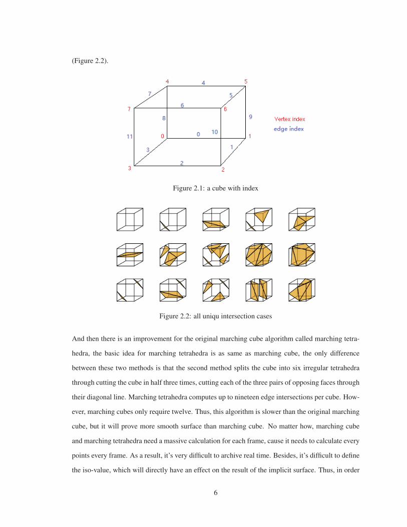
(Figure 2.2).

Figure 2.1: a cube with index

Figure 2.2: all uniqu intersection cases

And then there is an improvement for the original marching cube algorithm called marching tetra-

hedra, the basic idea for marching tetrahedra is as same as marching cube, the only difference

between these two methods is that the second method splits the cube into six irregular tetrahedra

through cutting the cube in half three times, cutting each of the three pairs of opposing faces through

their diagonal line. Marching tetrahedra computes up to nineteen edge intersections per cube. How-

ever, marching cubes only require twelve. Thus, this algorithm is slower than the original marching

cube, but it will prove more smooth surface than marching cube. No matter how, marching cube

and marching tetrahedra need a massive calculation for each frame, cause it needs to calculate every

points every frame. As a result, it’s very difficult to archive real time. Besides, it’s difficult to define

the iso-value, which will directly have an effect on the result of the implicit surface. Thus, in order

6

to have a better result, generally we need to add an additional smooth process for the marching cube,

which will slow down the algorithm once more. What’s more, all grid cells have to be visited to

establish a surface (Pascucci (2004)). However, visiting neighboring grid cells is not appropriate for

parallel computing, which means it not suitable for calculating on GPU, on which can outstanding

improve the speed. And then there is a way to render particle system through using the nature of the

particle systems which is that particle systems are ideal for exploiting temporal coherence. Once a

particle move into a surface of fluid at a particular time, it can be moved a small amount of distance

to represent the surface of fluid in a fraction of time later. This method called point-based surface

visualization introduced by GPU Gem3 (Nguyen (Sept. 12 2007)).

2.1.2 point-based surface visualization

The most important goal of this method is to use the as least as possible time to cover as much

surface as possible with the surface particles. This method not focusses on the rendering of the par-

ticles itself, instead, it focusses on treating blending of particles and shattering effects that create a

better surface. This method is built on a concept introduced by Witkin and Heckbert (1994) (Witkin

and Heckbert. (1994)) which is that an implicit surface can be sampled by restraining particles to

the surface and spreading out them across the surface. In order to implement this concept, three

things have to be done.

First, for purpose of constraining the particles on the fluid surface, the implicit function and its

gradient need to be efficiently evaluated. In order to restrain particles of an implicit surface produced

by fluid particles, they constrain the velocity of all particles so that they can only move with the

change of the surface. And as long as these particles don’t move away from the surface, they have

the freedom to move tangentially to the surface.

Second, with the purpose of getting a uniform distribution of surface particles, the repulsion forces

between the particles have to be computed. A uniform distribution is very important cause in order

to improve the speed of rendering. The number of overlap between particles should be minimized.

What’s more, for achieving a good result, the particles should cover the entire surface and should

7

not have holes or cracks. They achieve this goal through computing repulsion forces working on

the surface particles according to the SPH method.

Finally, they add another distribution algorithm, because the distribution coming from the repulsion

forces is too slow. Besides, it doesn’t work for distributing particles which are belonging disconnect

regions.

Figure 2.3 shows the overview of that method. Even though this method using fewer particles than

the previous marching cube and can be calculated on GPU. It still needs lots of calculation for each

frame. And with the number of particles increases with this method will become slower and slower.

Figure 2.3: The overview of the point-based surface visulaization

2.1.3 Image-Space 3D Metaballs

In order to get a better implicit surface a technique called metaball can be used. This method

was first introduced by Blinn (J.F.Blinn (1982)) for displaying molecular. The idea is visualising

molecules as isosurfaces when we do a simulation of a density field. In Blinn’s paper, they use the

exponential function:

D(r) = exp(−ar2) (6)

8

Where r is the distance between the current sampling particle and the centre of the current metaball.

The sum of the density functions of all particles weighted by the distance from the sampling particle

then generates the value of the density field. And then several field functions have been proposed,

like a degree four polynomial field functions in Mutrakami (Murakami and Ichihara. (1987)) or a

piecewise quadratic function by Nishimura (H. Nishimura and Omura. (1985)). Based on this basic

concept of metaball, a method using image-space to generate metaballs was proposed by Mller

(C. M and Ertl (2007)) was proposed.

A density field function was presented in that paper:

D(r) =16

9(1− (

r

2R)2)2 (7)

However,the density field function for this method was unlimited, as long as the function has a finite

support, an influence radius. Any threshold value can be chosen depending on the field function.

Occluded fragments are the most important problem need to be solved in generating metaball in

image space. There are two methods proposed in that paper, one is using an additional texture

to solve this problem which called Vicinity Texture, the other one solving the occlusion problem

through using multiple rendering passes called the walking depth plane.

Vicinity Texture: The metaballs can be rendered as point sprites in a single pass. And instead of

processing the whole image area, they process at the expense of an increased number of expensive

texture accesses (C. M and Ertl (2007)). They chose to attach the vicinity information of the vertices’

object space position rather than the screen position. In this way, their map can be view-independent

which means that only when the position of the vertices changes, the maps have to be updated. Thus,

they generate a texture which can hold the object space position and the radius of all other spheres

who will contribute to the density field. After having this lookup table for influencing sphere, the

desired sphere radius is passed as homogenous coordinate of the vertex. Using the sign of the

homogenous coordinate, they can determine whether the current sphere has the potential to form a

metaball. If it has that potential, they use a threshold value t to determine whether it actually can

form a metaball. They sample the density field within the influence sphere. The density function is

9

evaluated for both the current sphere and the spheres in the neighbour list. If the sum of the densities

is sufficiently close to the threshold t, the sampling ends.

The Walking Depth Plane: this method avoids using a texture based data structure, thus reducing

the calculation. The main idea of this method is to use multiple rendering passes with a moving

depth plane to approximate the isosurface. Two buffers are needed in this method, the first one,

λ− buffer, is utilized to store the depth information in image-space. It uses means of the distance

from the camera position in world space coordinates to approximate the isosurface. Besides, the

maximum distance which is employed to the termination criterion also stores in this buffer. The

second buffer is utilized to evaluate the density field. For the λ − buffer, first calculating the

starting and maximum depth values allover all spheres for each pixel. And then, uploading the

spheres as points with the influence radius of the density function. Next, evaluating the density

function at the position calculated by the depth information in λ − buffer and viewing ray of the

given pixel. The next step is moving the surface described by values in λ − buffer closer to the

isosurface of target and meanwhile updating values in λ− buffer. Therefore, two parameters have

to be decided, the direction of the step and the step size. The direction can be obtained directly from

the density value of the current pixel. If the density is less than the threshold, the direction should

be forward. The other way, if the density is greater than the threshold, then the direction should be

backward. In order to approximate the isosurface more precise, the step size should be decreased

when the density reaches the threshold. Two simple heuristics can be used as oracle which can be

used to control this decrease (C. M and Ertl (2007)):

|Δ| =

⎧⎪⎪⎪⎪⎨⎪⎪⎪⎪⎩

Δmax(1−D(x)2)) forD(x) < 1− ε

12Δmax(D(x)− 1) forD(x) > 1 + ε

0 otherwise

(8)

Δmax is the maximum step size which can be represented by the radius of smallest sphere, t is the

threshold, ε is the approximation tolerance, D(x) is the summed density at the position x. The last

thing needs to be considered is that when the loop should be terminated. Utilising the maximum

number and the size of the bounding box, the required iterations can be computed. However, the

10

required iterations have to be increased by a fixed number, cause the step size decreases adaptively.

In order to prevent overestimating the maximum number of iteration, a maximum execution time

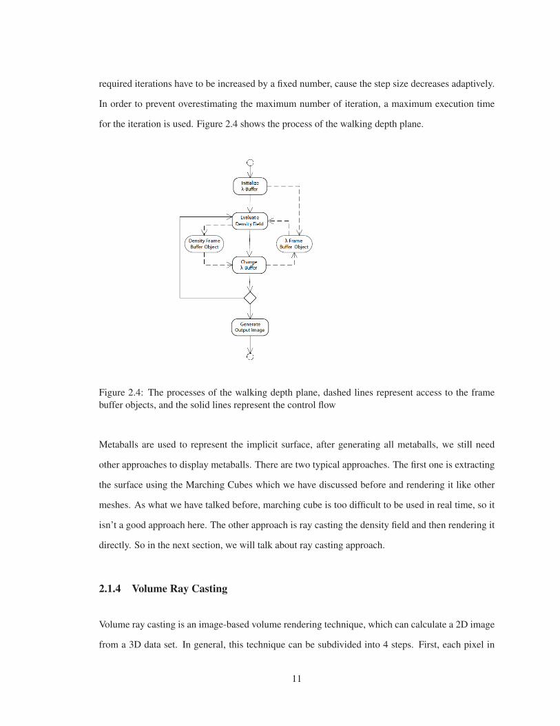
for the iteration is used. Figure 2.4 shows the process of the walking depth plane.

Figure 2.4: The processes of the walking depth plane, dashed lines represent access to the framebuffer objects, and the solid lines represent the control flow

Metaballs are used to represent the implicit surface, after generating all metaballs, we still need

other approaches to display metaballs. There are two typical approaches. The first one is extracting

the surface using the Marching Cubes which we have discussed before and rendering it like other

meshes. As what we have talked before, marching cube is too difficult to be used in real time, so it

isn’t a good approach here. The other approach is ray casting the density field and then rendering it

directly. So in the next section, we will talk about ray casting approach.

2.1.4 Volume Ray Casting

Volume ray casting is an image-based volume rendering technique, which can calculate a 2D image

from a 3D data set. In general, this technique can be subdivided into 4 steps. First, each pixel in

11

the final image will shoot a ray, these rays will pass through the volume. Second, taking samples or

sample points, along the ray that lies within the volume, cause not all volume points are directly on

the ray, so we need to take points which are located in between boxes. Thus, in order to get these

samples, we need to calculate them through interpolating values from their surrounding pixels.

Third, a gradient of illumination values for each sampling point needs to be calculated. These

gradients represent the orientation of volume’s surfaces. These samples are subsequently shaded

according to the surface orientation and the light-source location. Last, after shading all samples,

they will be composted along the ray. The color after the composition will be the final color on the

screen.

There is some ray casting method for metaballs. For example, a method introduced by Nishita and

Nakamae (NISHITA T. (1994)). In their algorithm, first, they calculate the intersections between

the viewing ray and each effective sphere, and then sort them depending upon the distance from the

viewpoint. Next, they find the isosurface for each interval on viewing ray according to the amount

of operational spheres intersected. If there is only one effective sphere intersected in the interval,

only one ray-sphere intersection test is needed, cause the isosurface is spherical. If there are two or

more effective spheres intersected, an equation in Bzier form need to be constructed, after extracting

metaballs intersected by the viewing ray. And they use Bzier clipping to solve it. Figure 2.5 shows

the basic framework for rendering metaballs.

And then a method which is an improvement of the previous method is introduced (Yoshihiro Kanamori

and Nishita (2008)). In this method, they only process the isosurface closest to the screen. In order

to achieve this goal, they utilize depth peeling to help. First they store the IDs of metalballs and

the distance between viewing point and the intersection point, called ray parameter, in a texture.

Meanwhile, they look up another texture which stores ray parameters from previous intersections,

if the parameters are less than the preceding ones the will discard this fragment. Besides, while

doing deep peeling, they split the screen into uniform tiles and doing depth peeling for each tile in

parallel. They compute which metaballs intersect with each file and store the intersecting metaballs

need to be rendered for each tile.

What’s more, they need to maintain a list of ray parameters and IDs of metaballs who will contribute

12

Figure 2.5: basic framework for rendering metaballs

to the isosurface. If a viewing ray intersected by an effective sphere twice, this effective sphere will

only contribute to the isosurface between those two intersections, so the metaball can be added to

the list of the first intersection point, and then be deleted at the list of the second intersection point,

figure 2.5 shows this process. Using this list, they will do ray interface text at each pixel using Bzier

clipping. And then, they repeat previous steps, using depth peeling to find an intersection and then

Figure 2.6: The process of maintaining a list based on the viewing ray in Figure 2.4

using Bzier clipping to do the ray isosurface testing, until isosurfaces is found or no intersection is

left. At last, shading the isosurface closest to the screen at each pixel.

13

Cause this method needs rendering effective spheres multiple times, they find a way to render oper-

ational spheres effectively. They only use the radii and centers of effective spheres to make them.

First, they identify the rectangular region which fits the perspective projected sphere on the screen.

Then, they do an intersection test for the operational sphere and the ray for each pixel in that region.

And then discarding the pixels which don’t have an intersection. This method only renders the front

or back surface of the sphere, however, they do not have to render them both with using depth peel-

ing. Only rendering the surface which is farther away from the aforementioned intersection point is

enough.

Next, for the purpose of reducing the number of rendered metaballs, they introduced a method which

will perform culling based on the fact that some metaballs will be hidden from the view point by the

metaballs that contribute to the isosurface, as shown in figure 2.7. First, they render the metaballs

who will contribute to the isosurface, called kernel sphere, and save the ray parameters to a texture.

And then, they stop writing to the depth buffer, and using the occlusion query to determine which

metaballs should be rendered.

Figure 2.7: metaballs with dash lines are hidden by the metaballs front

A new method which improves the speed of the sampling process is introduced in 2010 (Roland Fraedrich

(2010)). This method using a perspective grid which is generated through fix uniform grid to the

14

view volume. In the direct ray casting method, for each sample point, we need to interpolate the

neighbour point and doing the neighbour search for each sample point. Thus, we can store these

points into a cartesian grid to make the searching more effective. However, if we use a perspec-

tive grid,it will effectively reduce the number of primitives to be processed at run-time and also

the memory requirement. Figure 2.7 shows a perspective grid. The perspective grid will be used

to resample the particle data inside the view arrangement. The perspective grid is saved in a 3D

texture map. During the resample process, the quantities need to be revamped are scattered in this

3D texture map using accumulative blend.

In addition, in order to improve the speed and reduce memory access, they merge particles to a

user given resolution. This process is starting with a uniform grid based on the resolution that the

simulation has been performed. Particles in the range of 8 units of contiguous blocks are merged

into a single particle. And the volume of the new particle is the sum of the volumes of those

particles which have been merged. And the mass of this new particle is the average of merged

particles weighted by their mass. The merging process will be recursively repeated until reaching a

user given resolution.

2.1.5 Screen Space Rendering

Screen space rendering is introduced by Wladimir J. van der Laan. Simon Green and Miguel Sainz

in 2009 (Wladimir J. van der Laan (2009b)). This first part of our rendering model is based on this

method, cause first this method is fast enough to be done in real time. And second, after using this

method, we can somehow transfer the particle system to an object model. That is the result what

we want to get after the processing of the first step. Once we have this object model, we can do our

second step which will give the model a metal like rendering consequence very convenient. Besides,

it also can help us to get a high quality rendering result as ray casting. More details of this method

will be adopted in Chapter 3.

15

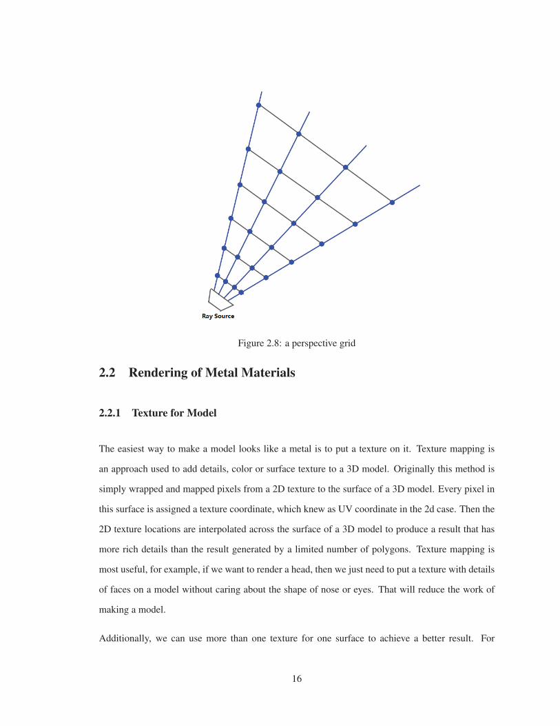
Figure 2.8: a perspective grid

2.2 Rendering of Metal Materials

2.2.1 Texture for Model

The easiest way to make a model looks like a metal is to put a texture on it. Texture mapping is

an approach used to add details, color or surface texture to a 3D model. Originally this method is

simply wrapped and mapped pixels from a 2D texture to the surface of a 3D model. Every pixel in

this surface is assigned a texture coordinate, which knew as UV coordinate in the 2d case. Then the

2D texture locations are interpolated across the surface of a 3D model to produce a result that has

more rich details than the result generated by a limited number of polygons. Texture mapping is

most useful, for example, if we want to render a head, then we just need to put a texture with details

of faces on a model without caring about the shape of nose or eyes. That will reduce the work of

making a model.

Additionally, we can use more than one texture for one surface to achieve a better result. For

16

Figure 2.9: add a texture to a 3D model

example, we can add a light map texture to light a surface as an replacement to recompute the light

each time rendering the surface. Bump mapping is a method to reach this. In bump mapping, it

allows a texture to control the facing direction of a surface for lighting computing directly. This

method can simulate small displacements of the surface without changing the surface geometry,

which will make the surface looks more realistic, as showed in figure 2.11. Bump map can be

Figure 2.10: sphere add a bump map appears to have more surface details

implemented through using a height map to simulate the surface displacement and generate the

modified normal. First, look up the height in the height map which corresponds to the position on

the surface, and then calculate the normal of the surface using this height. Next, combine normal

gotten from previous step and the normal of surface, as a result , new normal will point to a new

direction. And then using this new routine to calculate the light.

The other way to implement the bump map is using the normal map. In order to calculate the diffuse

lighting of a surface, unit vector normal to the surface is dotted with the unit vector from the shading

point to the light source, and the result is the intensity of the light on that surface. Through using a

bitmap with 3 channels across a model, normal vector information can be encoded. Each channel

in bitmap stores a spatial dimension. These spatial dimensions are corresponding to a coordinate

system for object space normal maps or a smoothly varying coordinate system. When using this

17

normal map, we need to look up the normal map for the normal and then the normal from tangent

space to world space or view space. The normal map process is shown in figure 2.12.

Figure 2.11: add normal map to an object

However, in our case, particle system has a dynamic shape, which means its shape changes with

frames. So it is very tough for us to use bump mapping or originally texture mapping. Cause map

textures are very difficult to generate. Thus, it’s very difficult for us to generate a metal surface

with lots of details, for example, worn surface with scar or brushed surface. However, we using the

roughness to make model looks more like metal. For the purpose of adding roughness, we utilizing

other kinds of texture mapping. In general, the texture mapping we use is environment mapping,

which can add a reflection of background to the 3D model. Through process, this reflection we

can generate the surface with different roughness. This technique will be introduced in details in

Chapter 4. What’s more, we also using mip-map to achieve different roughness. Based on different

roughness level, we will use different resolution images

2.2.2 Reflectance Models

In order to simulate a real-world metal material in a computer, a reflectance model which is used

to compute the interaction between light from a point on a surface and the incoming light need to

be defined. Reflectance models could be divided into two principal groups: theoretical models and

the empirical models. The empirical models provide computationally efficient reflectance models

which are lacking physical accuracy. Those models are limited and not accurate enough to be used

in a system which needs to get a result close to nature. However, these models are still popular

18

because its fast speed in some application does not require rendering physically accurate object.

The additional models, theoretical models, focus on providing physically accurate rendering result.

These models need much more computation than the empirical models which make them expensive

to render but they will provide a better result in terms of physically accurate rendering. This the-

sis focuses on rendering a physically accurate metal surface, so a theoretical reflectance model is

needed.

There is just an evolution of methods to simulate reflections in computer graphics in these years.

The first attempt to render a realism result in the computer is using a simple Lambertian reflectance

model. That method treats the surfaces as a perfectly diffuse surface, which means that the reflected

light is equally in each direction. In this case, no matter what direction the viewer is looking, the

surface will have the exact same appearance. Even though it is not physically possible to have a

perfect diffuser in nature, the Lambertian reflectance model could still be used to achieve a matte

look to a surface (Angel and Shreiner (2012)). An empirical model which can give more realism

and richness significantly is created by Phong in 1975 (Phong (n.d.)). This reflectance model can

give the surface a glossy-like appearance. This model combined by three parts: ambient parameter,

specular parameter and diffuse parameter.The ambient term represents a constant uniform color that

approximates light coming from the environment. The ambient parameter in the Phong equation is

a constant value that brightens up the entire object have to be rendered. However, in this case the

part in shadow won’t be totally black. The diffuse parameter is just like the Lambertian reflectance

model. The reflected light is equally in each direction. The specular parameter is used to simulate

highlight and describe the specular reflection which is the mirror-like reflection of light from a

surface. The equation for calculating the Phong reflection is (Phong (n.d.)):

Ip = kaia +∑

m ε light

(kd(Lm · N)id + ks(Rm · V)αis) (9)

Where is and id are intensities of specular and diffuse components of the light sources, ia is the

intensities of ambient lighting. This part sometimes calculated as the sum of all light sources. ks,

kd and ka are three constants for specular reflection, diffuse reflection and ambient reflection. They

19

Figure 2.12: Perfect diffuse, perfect specular and glossy specular

mean the ratio of reflection of the specular, the diffuse and the ambient. α is a shininess constant for

the material of the rendered object. With the increase of this ceaseless, the specular highlight will

become smaller. Moreover, textbfLm is the direction vector from the point on the surface toward

each light source, N is the normal at this point on the surface, V is the direction pointing towards

the viewer, Rm is the direction which is a reflected ray of light should take from this point on the

surface based on the law of reflection, it is computed as the reflection of Lm on the surface:

Rm = 2(Lm · N)N − Lm (10)

After this model, Jim Blinn developed a model based on the Phong’s model which decrease the

calculation. In this model, a halfway vector between the viewer and light-source vectors is used

20

instead of the reflection vector.

H =L + V

‖L + V‖ (11)

And then we can replace the (R · V)α to (N · H)α′, where α′ > α and α′ = 4α can have a good

result in specular highlights that very closely match the corresponding Phong reflections. Then the

equation to calculate the reflection becomes:

Ip = kaia +∑

m ε light

(kd(Lm · N)id + ks(N · H)α′is) (12)

The Blinn-Phong model is more efficient than the originally Phong model, cause it avoids computing

the more expensive calculation reflection vector R and it only needs to compute a more simple

vector. Blinn-Phong will be faster than Phong when the light-source and viewer are very remote.

This is true of directional lights. In this situation, the halfway vector can be treated as a constant.

Cause the halfway vector is only dependent on the incoming light direction and the direction of

the viewer position and they will individually converge cause the remote distance. Thus, H only

need to be calculated once for each light and don’t need to be changed if the view point and light

stay in the same relative position. However, this rule is not true for the Phong model, the reflection

vector R has to be recalculated for each vertex of the model. And after this improvement of Phong’s

Figure 2.13: direction vectors using in Phong model and Blinn-Phong model

21

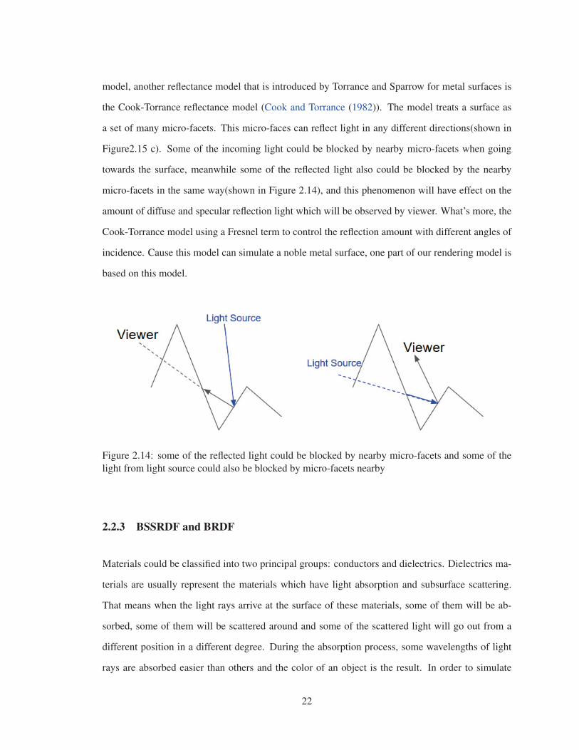
model, another reflectance model that is introduced by Torrance and Sparrow for metal surfaces is

the Cook-Torrance reflectance model (Cook and Torrance (1982)). The model treats a surface as

a set of many micro-facets. This micro-faces can reflect light in any different directions(shown in

Figure2.15 c). Some of the incoming light could be blocked by nearby micro-facets when going

towards the surface, meanwhile some of the reflected light also could be blocked by the nearby

micro-facets in the same way(shown in Figure 2.14), and this phenomenon will have effect on the

amount of diffuse and specular reflection light which will be observed by viewer. What’s more, the

Cook-Torrance model using a Fresnel term to control the reflection amount with different angles of

incidence. Cause this model can simulate a noble metal surface, one part of our rendering model is

based on this model.

Figure 2.14: some of the reflected light could be blocked by nearby micro-facets and some of thelight from light source could also be blocked by micro-facets nearby

2.2.3 BSSRDF and BRDF

Materials could be classified into two principal groups: conductors and dielectrics. Dielectrics ma-

terials are usually represent the materials which have light absorption and subsurface scattering.

That means when the light rays arrive at the surface of these materials, some of them will be ab-

sorbed, some of them will be scattered around and some of the scattered light will go out from a

different position in a different degree. During the absorption process, some wavelengths of light

rays are absorbed easier than others and the color of an object is the result. In order to simulate

22

this kind of material, an algorithm which can compute the light scattering is needed. Besides, some

dielectrics materials need more calculation cause they have more complex surface, for example,

complex multi-layered materials such as paper, skin, cloths and so on. Bidirectional surface scat-

tering reflection distribution function(BSSRDF) is developed for these materials. Such function is

considered computation heavy because the incoming light enters the surface. Scatters around inter-

nally, and exits the surface from a different place at a different angle (Jensen and Hanrahan. (n.d.)).

Figure 2.15: a. a bidirectional reflection distribution function(BRDF) - light incomes and outcomesat the same position. B. a bidirectional surface scattering reflectance distribution function(BSSRDF)the light incomes and outcomes at different places. C. A Cook-Torrance reflectance model whichtreats a surface as a set of many micro-facets, each facets has its own normal n.

However, metal is the material we need to render and metal is a conductor which is hardly translu-

cent and has very little subsurface scattering. Similarly with dielectrics, light rays arrive the surface

can be reflected or scattered. While the absorption for conductors is much stronger than dielectrics:

some of the light rays get reflected but the transmitted lights are absorbed almost immediately.Thus,

the main difference between dielectrics and conductors is that for conductors the light will income

23

and outcome in the same position.(as shown in Figure 2.15) In order to represent a surface be-

havior when interacting with light, a few variables need to be taken into account: incoming and

outgoing light angle, incoming and outgoing polarization, incoming and outgoing position, incom-

ing and outgoing wavelength and time delay between the incoming and outgoing light. Include all

those variables in the reflectance model will too expensive to calculate. Thus, a reflectance function

eliminating most variables and only retaining the incident and reflected light angles are generated.

Which is called bidirectional reflectance distribution function(BRDF). Instead using the more te-

dious calculation function BSSRDF, using BRDF can approximate the effect of BSSRDF, but the

light is assumed to income and outcome at the same position. That means BRDF don’t need to

spend many calculations for incoming and outgoing light directions, which simplify the computa-

tion. Among other materials, metals is under a very high level of reflectivity. When seeing a metal

material one could almost always recognize its metallic nature (Jensen and Hanrahan. (n.d.)). The

specular component is very important for metal, because it provides highlights which shows the

location relationship between light-source and rendered object and also the overall shape of that

object. Besides, the color of some metals changes based on their specular reflection while the non-

metal surface is usually having the same color with different specular reflection(shown in Figure

2.16).

Figure 2.16: In colored metals such as silver, aluminum, gold specular reflection changes their colorbased on thier properties. In this image, the metal bowl has a silver-gray colored highlight

24

2.2.4 Fresnel Term and Surface Reflectance

With different roughness of the surface, the direction of the outgoing light will have different be-

haviour for specular reflection. For a perfectly smooth surface which will make a perfect specular

reflection, the angle between the incoming light and the normal to the surface is same with the angle

between the normal and the outgoing light. This is the reflection law (shown in Fiture 2.17):

θi = θr (13)

On the other hand, for calculating refract ray, Snell’s law can be utilized. Snell’s law is built on

an index of refraction which describes how light propagates through that medium. Snell’s law

considers the index of refraction of both the medium of incident light and the medium of refraction

ray. The Snell’s law equation is:

nisinθi = ntsinθt (14)

Figure 2.17: reflected law and Snell’s law

Only calculating the specular reflection and refraction directions is not sufficient for the simulation.

25

It is still need to compute the amount of light that in reflection direction and in refraction direction.

However, for non-physical render models, they don’t have any resources for computing the amount

to reflect and refracted light. Instead, they using constant values for those parameters. On the other

hand, for physical render models, they using Fresnel equations to calculate reflected and refracted

light. For conductors and dielectrics, they have the equivalent Fresnel equation but with different

refractive indices. In order to facilitate the calculation, the light will be assumed unpolarized. And

then, perpendicular and parallel polarization terms need to be computed. For conductors, we need

an extra variable k for the imaginary part of the complex index of refraction. The Fresnel equation

is (Brennan (n.d.)):

Fr =r⊥ + r‖

2(15)

where the parallel and perpendicular terms are given by (Pharr and Humphreys. (2010)):

r⊥ =

∣∣∣∣∣∣n1cosθi − n2

√1− (n1

n2sinθi)2

n1cosθi + n2

√1− (n1

n2sinθi)2

∣∣∣∣∣∣2

r‖ =

∣∣∣∣∣∣n1

√1− (n1

n2sinθi)2 − n2cosθi

n1

√1− (n1

n2sinθi)2 + n2cosθi

∣∣∣∣∣∣2

(16)

Dielectrics have low reflectance for most of the angle and have an almost mirror-like near grazing

angles. On the other hand, conductors like metals have a very high reflective level. In general, shiny

metal surfaces have reflectance independent of angle. Usually, metals have reflectance of over 60%

for the whole angle while dielectrics have 20% or less for most of the angles (Westin and Torrance.

(n.d.)).(showed in Figure 2.18)

This Fresnel equation is a general equation, for our render model, we used Cook-Torrance Re-

flectance model which has a difference with the equation above. There is more than one Fresnel

approximation for Cook-Torrance. There are no obvious advantages or disadvantages for these ap-

proximations. In this thesis, we choose Schlick’s approximation which assumed that there is always

a perfect reflection, but the customary changes according to a certain distribution, resulting in a

26

Figure 2.18: showing the difference between dielectrics and metals. For dielectric materials onsurfaces have relatively low reflectance level of 20% or less for most of the angular range, whilemetals have a pretty high level of reflectance of 60% and above (Westin and Torrance. (n.d.))

non-perfect overall reflection.

2.2.5 Isotropic and Anisotropicls Surfaces

BRDF functions could be segregated into two classes: isotropic and anisotropic. The light re-

flectance that calculated by isotropic BRDFs remains unchanged when the surface is rotated about

its normal. Consider an object with a smooth surface and there are fixed light and viewer positions.

If we rotate the surface to its normal, the BRDF value which will have an effect on the final result

would remain unchanged. Materials with this feature such as smooth plastics usually use isotropic

BRDFs. On the other hand, the anisotropic BRDFs calculate light reflectance changed with the

rotation of the surface of its normal. For example the brushed metal or satin. Generally, most

real-world materials are anisotropic in some angle. Nonetheless, isotropic BRDFs is useful because

many real-world surfaces are probably more isotropic than anisotropic. The anisotropic effect on

some materials is so small that can be ignored in computer graphics simulations and can be used

isotropic BRDFs for approximation. Thus, in this thesis, we only using an isotropic BRDFs in our

rendering model.

27

Chapter 3

Screen Space Rendering Method

3.1 Generate Depth Image

In order to generate depth image which can be utilized easily in screen space rendering, a technique

called point sprites is needed. Because, representing points as small overlapped 2D images can

cause dramatic streaming animated filaments and if actually rendering sphere meshes at each point

the algorithm will become too expensive for the number of particles increase. Besides, using point

sprites will help us generate a sphere which is only rendered the part faces the camera which means

the opposite surface will not be rendered. Moreover, point sprites also can help us discard particles

which are ”below” the surface. First of all, drawing a quad for each particles, and then discarding

points outside the circle.

After this, in order to get a sphere like result, depth information need to be changed. The Formula

for a sphere is needed here.

x2 + y2 + z2 = 1

28

Figure 3.1: The viewer can only see a subset of the particles. Also, they can almost never see theopposing surface. These factors motivate the need for creating the surface in user’s perspective onlyand particles outside the viewer’s perspective are clipped.

Figure 3.2: turn the particles in Figure 2.1 into point sprites, the point always face the viewer

Figure 3.3: Point sprites which are ”below” the surface will not be rendered.

29

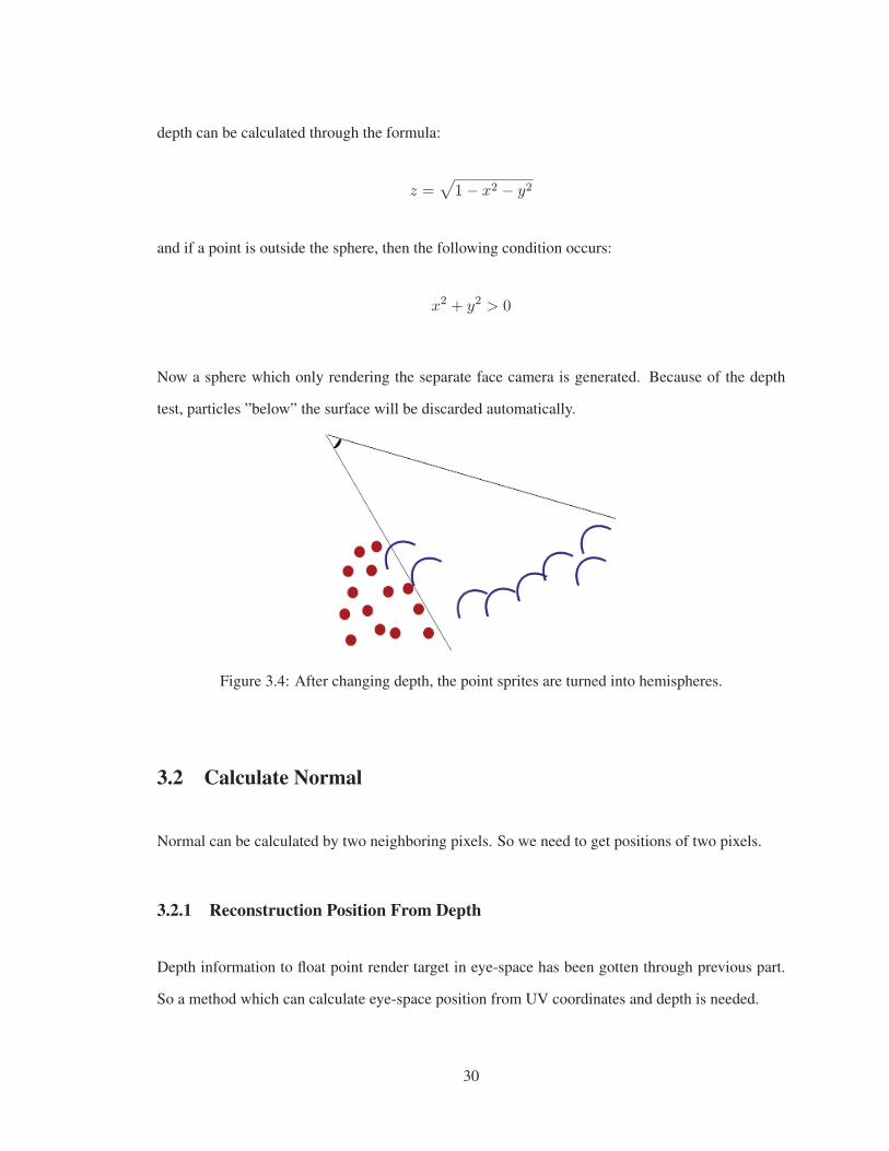
depth can be calculated through the formula:

z =√1− x2 − y2

and if a point is outside the sphere, then the following condition occurs:

x2 + y2 > 0

Now a sphere which only rendering the separate face camera is generated. Because of the depth

test, particles ”below” the surface will be discarded automatically.

Figure 3.4: After changing depth, the point sprites are turned into hemispheres.

3.2 Calculate Normal

Normal can be calculated by two neighboring pixels. So we need to get positions of two pixels.

3.2.1 Reconstruction Position From Depth

Depth information to float point render target in eye-space has been gotten through previous part.

So a method which can calculate eye-space position from UV coordinates and depth is needed.

30

Figure 3.5: This figure shows the result of depth image

2D position of the pixel is now got, which means if we can sample a depth value the whole 3D

position will be gotten. There is a very easy way to be involved if we have the access of hardware

depth buffer. First, storing post-projection z/w, and then, combining it with x/w and y/w, then,

transforming by the inverse of the projection matrix and dividing by w. Then a whole 3D position

is reconstructed.

3.2.2 Calculate Normal

Once we can have the entire 3D position information of each pixel, normal can be calculated through

partial differences of depth. First, we pick the pixel at the center pixel’s right side and then calcu-

lating the spatial difference between them called ddx. Next, we pick the pixel upper the center

pixel and then calculating the spatial difference between them called ddy. Then the normal is cross

product by ddx and ddy.

But normal may not be well-defined at the edges, because the center pixel maybe don’t have the

31

Figure 3.6: the normal is the cross product between ddx and ddy

pixel upper or at it right side. In this case, opposite direction must be used. So in order to get well-

defined normal at edges, we need to calculate the upper pixel center pixel and at right side of center

pixel and their opposite direction which is under the center pixel and at the left side of the center

pixel. And then we need to calculate the difference between upper pixel and center pixel called

ddy and the difference between center pixel and the pixel at it right side called ddx. Besides, the

difference between under pixel and center pixel called -ddy and the difference between center pixel

and the pixel as it left side called -ddx need to be calculated either. Moreover, we need to compare

the absolute between ddy.z and -ddy.z and also the absolute between ddx.z and -ddx.z. Then we will

choose the smaller one. The smaller one means this side is in the picture, to do the cross product

and calculate the normal.

Figure 3.7: The normal image calculated through depth image

32

3.3 Smooth Depth Image

For this part, two filters can be chosen, the first one is the Gaussian blur. The second one is the

bilateral blur.

3.3.1 Gaussian Blur

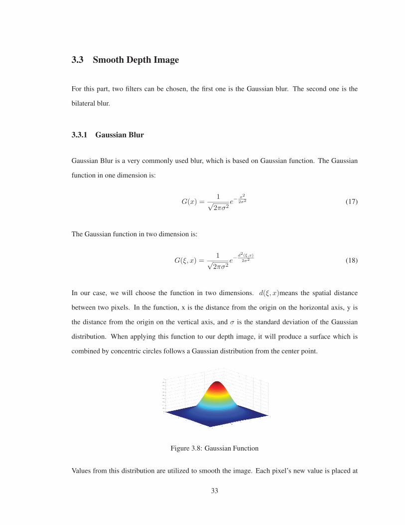
Gaussian Blur is a very commonly used blur, which is based on Gaussian function. The Gaussian

function in one dimension is:

G(x) =1√2πσ2

e−x2

2σ2 (17)

The Gaussian function in two dimension is:

G(ξ, x) =1√2πσ2

e−d2(ξ,x)

2σ2 (18)

In our case, we will choose the function in two dimensions. d(ξ, x)means the spatial distance

between two pixels. In the function, x is the distance from the origin on the horizontal axis, y is

the distance from the origin on the vertical axis, and σ is the standard deviation of the Gaussian

distribution. When applying this function to our depth image, it will produce a surface which is

combined by concentric circles follows a Gaussian distribution from the center point.

Figure 3.8: Gaussian Function

Values from this distribution are utilized to smooth the image. Each pixel’s new value is placed at

33

a weighted average of that pixel’s neighborhood. The original pixel’s value will have the heaviest

weight and neighboring pixels will have smaller weights with their distance to the original pixel

grows. Equation 2.3 shows the Gaussian Blur in a continuing situation.

h(x) = k−1r (x)

∫ ∞

−∞

∫ ∞

−∞f(ξ)G(ξ, x)dξ (19)

kr(x) =

∫ ∞

−∞G(x)dξ (20)

kr(x) is used to unitize the result. In order to use Gaussian blur in our depth image, Gaussian

function needs to be discredited. In theory, the whole picture will be included in the Gaussian

calculation for each pixel, because there is no zero value in the picture. Nonetheless, it is too

expensive for calculation. Actually, we only need to consider neighbors which have distance smaller

than 3σ, cause neighbors outside this distance are so small that can be considered as zero. After

discretization, we will get a Gaussian function in discrete situation.

h(x) = k−1r (x)

∑Ω

f(ξ)G(ξ, x)dξ (21)

The consequence picture shows a problem caused by Gaussian Blur, which is the edge of the object

becomes dimmed. So a new blur method will be introduced which is bilateral blur.

3.3.2 Bilateral Blur

Bilateral blur can be seemed as an improvement of Gaussian Blur. The most important improvement

is that the bilateral blur can keep edge information. Gaussian blur only use spatial difference to

generate weight factor, so the edge information will loss during the process. The edge information

here means the edge between different color area, for example, the edge between blue sky and the

gray house. So for bilateral blur, it will consider both spatial difference and similarity between

34

pixels. And the bilateral blur function becomes this

h(x) = k−1(x)

∫ ∞

−∞

∫ ∞

−∞f(ξ)G(ξ, x)C(f(ξ), f(x)) (22)

Also this continuous function can’t use in our depth image we still need to make it into discrete

situation.

h(x) = k−1r (x)

∑Ω

f(ξ)G(ξ, x)C(f(ξ), f(x))dξ (23)

Figures 3.8 can show the difference between Gaussian and bilateral more obvious.

Figure 3.9: blue quad is the position of center pixel, middle figure is the shape of Gaussian blur,right is the shape of Bilateral blur

Similarity Weight

Spatial weight has been discussed in Gaussian Blur part. Now we will discuss about similarity

weight which is the most important improvement from Gaussian Blur. It is similar with spatial

weight, instead of considering the spatial distance between pixels, we will use the difference in

depth to calculate the similar weight.

s(ξ, x) =1√2πσ2

e−σ2(f(ξ),f(x))

2σ2 (24)

35

σ(f(ξ), f(x))means the difference of depth between two pixels.

Figure 3.10: A shows the normal image calculated through the depth image smoothed by GaussianBlur. B shows the normal image calculated through the depth image smoothed by Bilateral Blur.We can find out that the edges of the object in the image smoothed by Gaussian Blur have morenoise than one smoothed by Bilateral Bulr

36

3.3.3 Adaptive Kernel Size

Smooth deep image is a very expensive step, so in order to have a better performance a method

which can make this step faster is needed. There is a very easy way to get this goal, which is

adaptive change the kernel size of the filter. Kernel size makes a significant contribution of the

running time, so decline the kernel size will improve the performance obviously. In our case, we

change the kernel size built on the distance between the screen and the object. If the object is far

from the screen then we will use a small kernel size and if the object is, near the screen we will use

a larger kernel size. But the kernel size can be increased unlimited cause as the discussion before,

when a pixel is too far from the center pixel, the effect of this pixel is too small to be calculated.

And the best kernel size is nothing more than 3 ∗ σ. And then we have a function to calculate the

kernel size.

ks =

⎧⎪⎪⎪⎪⎪⎪⎨⎪⎪⎪⎪⎪⎪⎩

3 ∗ σ d <= threshold

3 ∗ σ − d ∗ k d > threshold

ksmin ks < ksmin

(25)

d is the distance between the object and the screen space. This can be obtained easily through depth.

k is the kernel size decline rate and ksmin is the minimal kernel size. Threshold is the threshold to

judge whether we are required to decrease the kernel size.

3.3.4 Adaptive Particle Ratio

In screen space rendering method, particle ratio is a very important parameter need to be dealt with

very carefully. Cause if we use a large particle ratio we will have more flat surface, but we will

lose some feathers in surface. On the other hand, if we use a small particle ratio the feathers of the

surface can be preserved, but the surface won’t be very flat. And for water, the splash particle won’t

need big particle ratio, also for welding, particles drop from work pieces won’t need heavy particle

ratio. On the other hand, both work pieces and the whole water body need large particle ratio to

keep them flat. In order to satisfy different demand, we must have different particle ratio at the same

37

time. Thus, a method which can adjust particle ratio based on the status of particles is required.

In this paper, a method based on color field is developed. Color field is a parameter which can be

utilized to judge whether a particle is belong to surface.

Color Field

This quantity is built on SPH, which means it should be calculated during the SPH simulation. First,

in order to define the surface of the fluid, a quantity called the color field is used to define the shape

of fluid.

c =∑j

mj

ρjW (r − rj) (26)

Where m means the mass of the particle and ρ is the density of the particle, W() is a kernel function

and r means kernel ratio. This also can be looked at the weighted ”volume” from each particle.

The normal of a surface can be defined using this function, as the gradient of the color field. The

direction in which color is most increasing points toward the surface. We do not have to use the

kernel function which is modified for specific behavior in the gradient or laplacian, standard kernel

function is enough.

n =∑j

mj

ρj�W (r − rj) (27)

A particle can be identified as a surface particle if its customary length exceeds a certain threshold.

|n| < tnormal (28)

Adaptive Particle Ratio

After identified surface particle, we can calculate the adaptive particle ratio. First, we calculate the

average density of the surface particle and then we use this average density called surface density

38

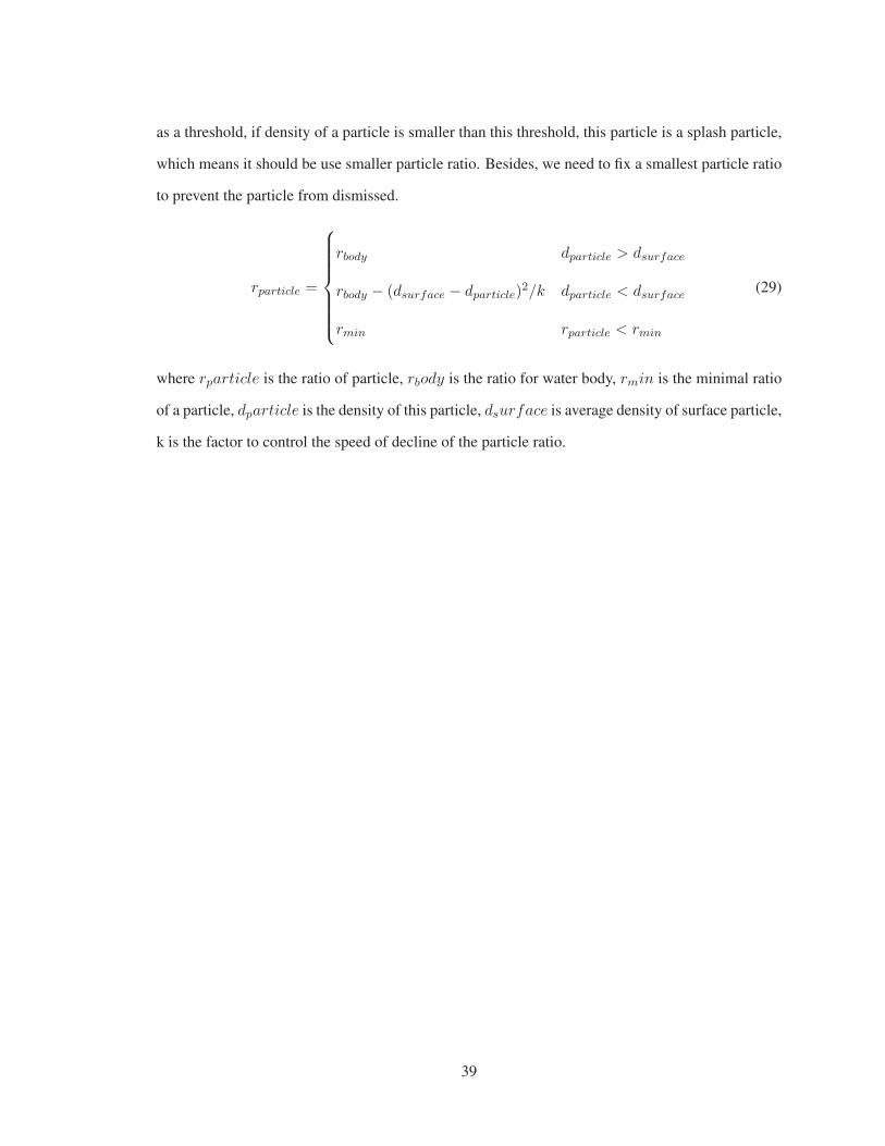
as a threshold, if density of a particle is smaller than this threshold, this particle is a splash particle,

which means it should be use smaller particle ratio. Besides, we need to fix a smallest particle ratio

to prevent the particle from dismissed.

rparticle =

⎧⎪⎪⎪⎪⎪⎪⎨⎪⎪⎪⎪⎪⎪⎩

rbody dparticle > dsurface

rbody − (dsurface − dparticle)2/k dparticle < dsurface

rmin rparticle < rmin

(29)

where rparticle is the ratio of particle, rbody is the ratio for water body, rmin is the minimal ratio

of a particle, dparticle is the density of this particle, dsurface is average density of surface particle,

k is the factor to control the speed of decline of the particle ratio.

39

Figure 3.11: A shows the result with adaptive ratio, B shows the result without adaptive ratio

40

Chapter 4

Physically Based Rendering

In order to make the result of rendering similar with metal, we need to simulate the light reaction

of metal which means we need to use a light simulation method which can get a similar result with

metal reflection. Physically based rendering is choosed to achieve our goal.

4.1 Rendering Equation

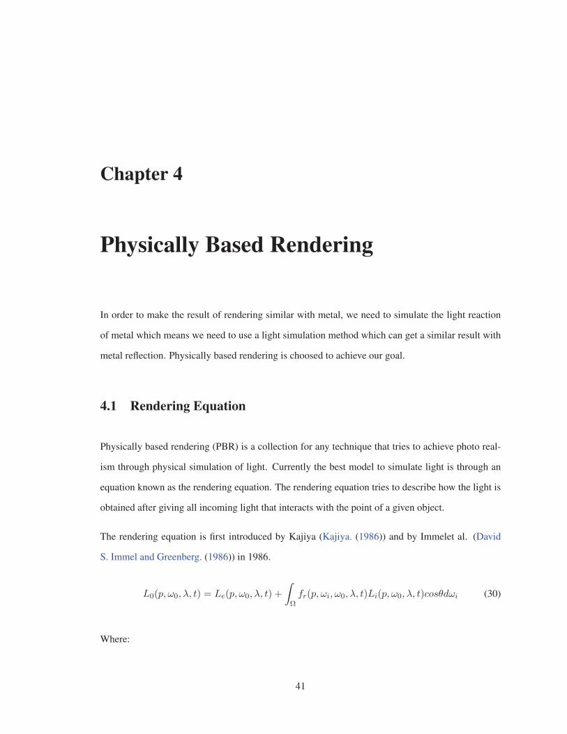
Physically based rendering (PBR) is a collection for any technique that tries to achieve photo real-

ism through physical simulation of light. Currently the best model to simulate light is through an

equation known as the rendering equation. The rendering equation tries to describe how the light is

obtained after giving all incoming light that interacts with the point of a given object.

The rendering equation is first introduced by Kajiya (Kajiya. (1986)) and by Immelet al. (David

S. Immel and Greenberg. (1986)) in 1986.

L0(p, ω0, λ, t) = Le(p, ω0, λ, t) +

∫Ωfr(p, ωi, ω0, λ, t)Li(p, ω0, λ, t)cosθdωi (30)

Where:

41

* λ is a particular wavelength of light t is time

* t is time

* p is the location in space

* n is the surface normal at that location

* ω0 is the direction of the outgoing light

* ωi is the negative direction of the incoming light

* Le(p, ω0, λ, t) is emitted spectral radiance

* Ω is the unit hemisphere centered at n containing all values for ωi

* Li(p, ω0, λ, t) is spectral radiance

* fr is the bidirectional reflectance distribution function

* L0(p, ω0, λ, t) is the total spectral radiance of λ directed outward along direction ω0 at time

t, from a position p

We do not need to solve the whole rendering equation, because time, wavelength and emitted radi-

ance will not need to be considered in our case. Thus a simplified version of rendering equation is

enough.

L0(p, w0) =

∫Ωfr(p, wi, w0)Li(p, wi)(n · wi)dwi (31)

This equation gives us the colour of a pixel after considering all incoming light and also tell us how

to mix them. The equation describes the outgoing radiance from a point L0(p, ω0), which is used to

color a pixel on screen.

To calculate it, the normal of surface where pixel lies on is needed. The dot product n · ωi is used

to take into account the angle of incidence angle of the light ray, which is the component cosθ in

42

Figure 4.1: The rendering equation is used to describe the light emitted from a position x along aparticular viewing direction, using a BRDF and incoming light.

equation (4.1). If the light ray is perpendicular to the surface, it will be more localized on the surface

of object, on the other hand, if the angle is small it will be spread across a bigger area, eventually

spreading too much to be observed.

In a word, this equation is simply calculating the outgoing radiance through the given incoming

radiance which is weighted by the angle between every incoming light and the normal of the surface.

The other part of the equation we need to talk about is fr(p, ωi, ω0). It is bidirectional reflectance

distribution function(BRDF) that we have mentioned before. This function is used to output a

weight of how much the incoming light is contributing to the final result after considering position,

incoming and outgoing radiance. It is the most important component in this function also in physics

based rendering. Through choose different BDRF, different kind of material can be simulated. As

what have been mentioned before, light refection can be separated by two parts: specular reflection

and diffuse reflection. BRDF is the factor used to calculate them. For a perfectly specular reflection,

for instance, mirror, the BRDF is 0 for every incoming light except the one that has same angle of

the outgoing light whose BRDF is 1. It’s important to notice that a physically based BRDF have to

respect a law which is:

∀ωi

∫Ωfr(p, ωi, ω0)(n · ωi)dω0 ≤ 1 (32)

it means that the sum of reflected light must not exceed the amount of incoming light.

43

4.2 Light in PBR

Computing lighting in PBR is as same as the calculating in current rendering system, which means

we need to calculate ambient, diffuse, specular. For each light source, computing the specular factor

and diffuse factor. BRDF will help calculate this factor more physically accurate. So for different

light sources and different light factor, different BRDF will be choosing.

Light source can be divided into two classes through direction: direct light source and indirect light

source

Direct light source means a source emitted light through a certain direction, the most common light

sources are directional lights, spot lights and point lights.

Indirect light source means a source which can reflect light and indirectly lights to its surrounding

object. In our case, we use environment map as a light source. In this paper, we use a technique

called Image Based Lighting(IBL) to achieve our goal.

4.2.1 Direct Light

In this section, the BRDF which is used to deal with direct light will be presented. The light can be

separated by diffuse factor and specular factor, so we choose different BRDF for each factor.

Diffuse BRDF: Lambert

Lambert is a very common and simple way to compute the diffuse reflection. This technique makes

all closed polygons have same reflect light in all directions. The equation for this BRDF is:

fLambert(p, ωi, ω0) =Cdiff

π(33)

Where Cdiff is the diffuse albedo of the material.

44

Figure 4.2: a bunny rendered with direct diffuse light

Specular BRDF: Cook-Torrance

Cook-Torrance is a very useful BRDF for computing specular reflection. This technique was intro-

duced by Cook and Torrance in 1982 (Cook and Torrance (1982)). The Cook-Torrance model is

closer to physical reality than the Phong or Blinn-Phong models (Blinn (1977)). The basic idea of

this method is that treating each surface as combined by many micro facets: which is very small

facets can reflect incoming light. The general model of Cook-Torrance is:

fcook−torrance =DGF

4(n · l)(n · v)(34)

where D means distribution function, G means geometry function, F means fresnel function, n

means normal, v means the vector toward the viewer the viewing direction, l means the light vector.

D, G, F are the basis for cook-torrance, they are used to describe the behaviour of micro facets in

reflection and all of them are statistical models.

Fresnel Function F

F is used to simulate how the light will reflect with a surface in different angles. Fresnel is used

to calculate how much of light reflects based on the current angle between the incoming light and

the normal. As the incident angle becomes larger, the amount of light which reflects into our eyes

45

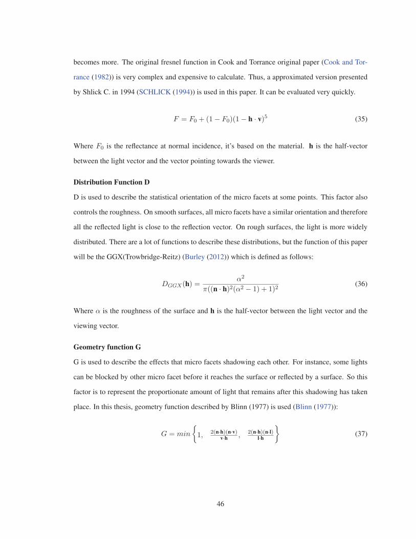
becomes more. The original fresnel function in Cook and Torrance original paper (Cook and Tor-

rance (1982)) is very complex and expensive to calculate. Thus, a approximated version presented

by Shlick C. in 1994 (SCHLICK (1994)) is used in this paper. It can be evaluated very quickly.

F = F0 + (1− F0)(1− h · v)5 (35)

Where F0 is the reflectance at normal incidence, it’s based on the material. h is the half-vector

between the light vector and the vector pointing towards the viewer.

Distribution Function D

D is used to describe the statistical orientation of the micro facets at some points. This factor also

controls the roughness. On smooth surfaces, all micro facets have a similar orientation and therefore

all the reflected light is close to the reflection vector. On rough surfaces, the light is more widely

distributed. There are a lot of functions to describe these distributions, but the function of this paper

will be the GGX(Trowbridge-Reitz) (Burley (2012)) which is defined as follows:

DGGX(h) =α2

π((n · h)2(α2 − 1) + 1)2(36)

Where α is the roughness of the surface and h is the half-vector between the light vector and the

viewing vector.

Geometry function G

G is used to describe the effects that micro facets shadowing each other. For instance, some lights

can be blocked by other micro facet before it reaches the surface or reflected by a surface. So this

factor is to represent the proportionate amount of light that remains after this shadowing has taken

place. In this thesis, geometry function described by Blinn (1977) is used (Blinn (1977)):

G = min

{1, 2(n·h)(n·v)

v·h , 2(n·h)(n·l)l·h

}(37)

46

BDRF for direct light

We now have got the diffuse part and specular part of direct light, and then combine them will give

us the whole function for direct light. The BRDF after combining is:

fr = kdfLambert + ksfcook−torrance

= kdCdiff

π+ ks

DGF

4(n · l)(n · v)

(38)

And then we use this function into our rendering equation(4.1):

L0(p, l) =

∫Ω(kd

c

π+ ks

DFG

4(l · n)(v · n))Li(p, l)(n · l)dl

= kdc

π

∫ΩLi(p, l)(n · v)dv + ks

∫Ω

DFG

4(l · n)(v · n)Li(p, l)(n · l)dl

(39)

Now we have the function to calculate all light reflection caused by direct light. The last things

we need to calculate are two weights kd and ks. Since these weights represent the amount of light

reflected, it similar with fresnel. Thus, we can use fresnel itself for ks and then, because the energy

conservation law, ks + kd = 1, we can obtain kd as kd = 1− ks.

Figure 4.3: a bunny rendered with direct light

47

4.2.2 Indirect Light

Indirect light also can be treated as ambient light, which will come from every direction, instead

of one direction. A very common way to deal with indirect light is to use environment map as the

indirect light source. And because of the environment is combined by images this light also called

image based light(IBL).

Environment Map

Cube map is a very common and useful environment map, first introduced by Greene, N. (Greene

(n.d.)). This method uses the six faces of a cube as the map shape. The environment will be projected

onto each side of the cube. They will be combined into a single texture with six regions or be stored

as six square textures. Comparing with other mapping method, for instance, sphere mapping, cube

map its relative simplicity and can use both the entire resolution and lower resolution images.

We can use simple reflect rule to fetch a pixel from an environment map.

Figure 4.4: known view ray and normal we can calculate reflect ray

This is useful for specular reflection, but we can’t use this for diffuse reflection. Reason for indirect

48

light, the light is coming from everywhere. Technically, every pixel in the environment map is a light

source, so a shaded point is lighted by a vast amount of pixels. This process also called irradiance

mapping. From figure 4.2, in order to calculate the diffuse reflection we need to fetch all pixels on

Figure 4.5: orange area represent the light rays coming from the environment to the shaded pixel.

cube map and combine the color for each shaded pixel, that will be a very expensive for a real time

rendering method. In this paper, we use a method which based on Spherical Harmonics

Spherical Harmonics lighting

The function we used to model the illumination is very similar with the equation(4.2), which is:

En(n) =

∫Ω(n)

L(ω)(n · ω)dω (40)

E is a function of the surface normal only and is given by an integral over the upper hemisphere

Ω(n). Besides, nandω are unit direction vectors, so E and L can be particularized by a direction

(θ, φ) on the unit sphere.

The spherical harmonics function Yl,m(θ, φ), with l ≥ 0and − l ≤ m ≤ l, are a set of orthogonal

49

functions defined on the unit sphere. These functions are defined as follows:

Y ml (θ, φ) = NeimφPm

l (cosθ) (41)

where Pml (x) is the m th Legendre polynomial of order l and N is a normalization factor that

depends on l and m.

Because the spherical harmonic functions are orthonormal on the unit sphere, any function defined

on the unit sphere can be described as a linear combination of spherical harmonics, then we can

change our equation 4.12 to a spherical harmonic form (Ramamoorthi and Hanrahan (2001a)):

E(θ, φ) =∑l,m

ElmYlm(θ, φ) (42)

For rendering, cause we only need diffuse information, so only low-frequency lighting coefficients,

with withl ≤ 2, is needed. Equivalently, the irradiance is well approximated by only 9 parameters

(Ramamoorthi and Hanrahan (2001a)). The first 9 spherical harmonics(with withl ≤ 2) are simply

constant(l = 0), linear(l = 1), and quadratic(l = 2) polynomials of the cartesian components(x, y, z)

(Ramamoorthi and Hanrahan (2001a)):

(x, y, z) =(sinθcosφ, sinθsinφ, cosθ)

Y00(θ, φ) =0.282095

(Y11;Y10;Y1−1)(θ, φ) =0.488603(x; z; y)

(Y21;Y2−1;Y2−2)(θ, φ) =1.092548(xz; yz;xy)

Y20(θ, φ) =0.315392(3z2 − 1)

Y22(θ, φ) =0.546274(x2 − y2)

(43)

One more parameter we need to solve the equation 4.14 is Elm:

El,m =

√4π

2l + 1AlLlm (44)

50

In order to simplify this equation we define a new variable A′l by

A′l =

√4π

2l + 1Al (45)

An analytic formula for Al is introduced by (Ramamoorthi and Hanrahan (2001b)) and based on

that formula we can calculate the A′l by:

l = 1 A′l =

2π

3

l > 1, odd A′l = 0

l even A′l = 2π

(−1)l2−1

(l + 2)(l − 1)

[l!

2l( l2!)2

] (46)

As we mentioned before, we only need the parameters with 0 ≤ l ≤ 2, so we only need the first

three A′l which are : A′

0 = π,A′1 =

2π3 , A′

2 =π4 .

The only parameter needed to be calculated is 9 lighting coefficients Llm, with l ≤ 2, which comes

from a given environment map.

Llm =

∫ π

θ=0

∫ 2π

φ=0L(θ, φ)Ylm(θ, φ)sinθdθdφ (47)

The expressions for the Ylm can be founded in equation 4.15. And it’s easy to notice that Llm is

independent of the normal direction n, which means we can precipitate the Llm before rendering,

that is the key to compute En quickly and efficiently when we need it in rendering process. Since

the values L(θ, φ) are computed through doing lookups in a given environment map, we can reduce

the Llm integral to a sum over pixels in the environment map:

Llm =∑i

LiYlm(ωi)dωi (48)

And we also can change the En function to a normal based form:

En =

2∑l=0

1∑m=−1

ElmYlm(n) (49)

51

All in all, for the whole method, first we use spherical harmonic function to calculate spherical har-

monic coefficient Llm from a given environment, and then we use Llm and A′l to combine Elm,next,

we use Elm and spherical harmonic function to inverse the light in real time, in the end, we will get

a diffuse light based on environment map.

Figure 4.6: a bunny rendered with diffuse light calculated through Spherical Harmonics

Specular Reflection with Roughness

In order to calculate specular reflection we can use the method we mentioned before (4.2.3.1) but

it can only give us a smooth surface effect. However, metal surface won’t be always smooth, we

need to have the ability to simulate more blurry surface which will make the model more realistic.

Thus, we need the reflection to be more blurry as the roughness increase. The basic idea is to store

different levels of roughness in the environment map mipmaps. Which means the first mipmap level

will match roughness 0 and the last will match roughness 1. Besides, in order to make the result

more blurry we can’t only fetch one pixel from the environment map, instead, we will sample a few

pixels and then combine them together as the figure 4.3.

In order to do archive this goal, we using importance sampling, which is a general technique for

estimating properties of a particular distribution, while only having samples generated from a dif-

ferent distribution than the distribution of interest. We use Hammersley points to get these random

samples.

52

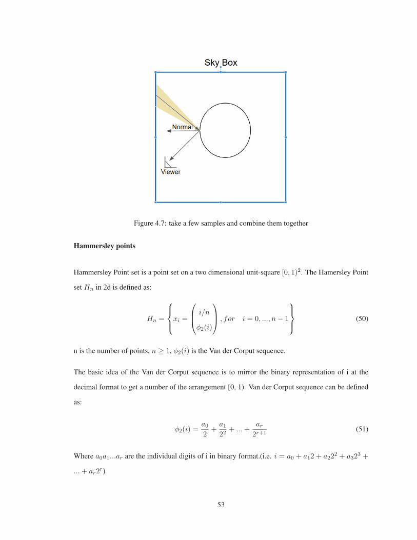
Figure 4.7: take a few samples and combine them together

Hammersley points

Hammersley Point set is a point set on a two dimensional unit-square [0, 1)2. The Hamersley Point

set Hn in 2d is defined as:

Hn =

⎧⎪⎨⎪⎩xi =

⎛⎜⎝ i/n

φ2(i)

⎞⎟⎠ , for i = 0, ..., n− 1

⎫⎪⎬⎪⎭ (50)

n is the number of points, n ≥ 1, φ2(i) is the Van der Corput sequence.

The basic idea of the Van der Corput sequence is to mirror the binary representation of i at the

decimal format to get a number of the arrangement [0, 1). Van der Corput sequence can be defined

as:

φ2(i) =a02

+a122

+ ...+ar2r+1

(51)

Where a0a1...ar are the individual digits of i in binary format.(i.e. i = a0 + a12 + a222 + a32

3 +

...+ ar2r)

53

As showed in figure 4.4, the points are well distributed in a unit square [0, 1)2. After getting well

distributed points set, next we need to transfer this points to a hemisphere.

Figure 4.8: 25 Hammersley points in a unit square

Generating Points on the Hemisphere

To create directions on the hemisphere from Hn, we can use cosine weighted distribution on the

sphere. Let xi =

⎛⎜⎝s

t

⎞⎟⎠ ∈ Hn be a point from Hammersley point set. Now we can calculate from

two coordinates s and t (Wong, Luk, and Heng (1997)):

θ =cos−1(√(1− s))

φ =2πv

VHemisphere =(cosφsinθ, sinφcosθ, cosθ)

(52)

Calculate Specular Light

After having the vector on hemisphere, we can use these vectors as the new normal which is rotated

from the original normal. We have known the view vector which can help us calculate the light

54

direction:

L = 2h(v · h)− v (53)

Where L is the light direction we need to calculate, h is the direction we get from Hammersley

points set, v is the view direction.

And then we can use this light direction to fetch pixels from an environment map shown in figure

4.5. Besides, after knowing each light direction we need to calculate, we can treat them separated

which means we can treat them like direct light which we mentioned before. Thus, we can calculate

their BDRF using the method we discussed in previous sections. At last, we combine all samples

we get together, then, we will get our final result for indirect specular light.

Figure 4.9: take samples from environment based on the Hammersley Vector

4.3 Final Lighting Calculate

Similar with the direct light calculation previously, at last, we only need to combine the diffuse light

and the specular light for indirect light:

Lindirect = kdLinDiff + ksLinSpec (54)

55

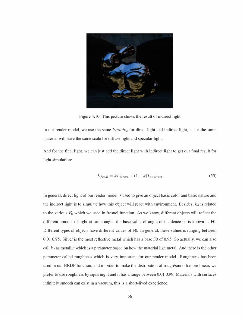
Figure 4.10: This picture shows the result of indirect light

In our render model, we use the same kdandks for direct light and indirect light, cause the same

material will have the same scale for diffuse light and specular light.

And for the final light, we can just add the direct light with indirect light to get our final result for

light simulation:

Lfinal = kLdirect + (1− k)Lindirect (55)

In general, direct light of our render model is used to give an object basic color and basic nature and

the indirect light is to simulate how this object will react with environment. Besides, kd is related

to the various F0 which we used in fresnel function. As we know, different objects will reflect the

different amount of light at same angle, the base value of angle of incidence 0◦ is known as F0.

Different types of objects have different values of F0. In general, these values is ranging between

0.01 0.95. Silver is the most reflective metal which has a base F0 of 0.95. So actually, we can also

call kd as metallic which is a parameter based on how the material like metal. And there is the other

parameter called roughness which is very important for our render model. Roughness has been

used in our BRDF function, and in order to make the distribution of rough/smooth more linear, we

prefer to use roughness by squaring it and it has a range between 0.01 0.99. Materials with surfaces

infinitely smooth can exist in a vacuum, this is a short-lived experience.

56

Chapter 5

Conclusion and Discuss

In this thesis, we combine two techniques to develop a render model for particle systems. With our

render model, particle systems can have a metal-like surface which makes these systems work in the

simulation referring to metal, like welding. Our render model can work for particle system, so we

can have a simulation of liquid metal as shown in Figure 5.1. Besides, we can represent object with

particles, so we can render the object which can change shape very easily, like welding application,

our rendering model can be used in welding very conveniently.(shown in Figure 5.2). In addition,

we can have object or liquid metal with different roughness as shown in Figure 5.4. And here is a

video shows the result.

Figure 5.1: a liquid metal with background reflectance

57

Figure 5.2: A shows a bunny constructed by particles. B shows a melting process with that bunny

Figure 5.3: two metal bars are wielded together.

5.1 Future Work

As we have mentioned before, because of the nature of particle system, it is very difficult to put

textures on particle system. However, if we can put textures on particle system, we can have a much

better result with more surface details, such as scars, brushed metal effect. So it is better to find

a method which can add texture to particle system and combine it in our render model. Besides,

58

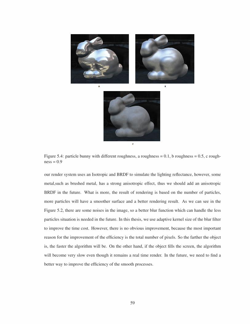
Figure 5.4: particle bunny with different roughness, a roughness = 0.1, b roughness = 0.5, c rough-ness = 0.9

our render system uses an Isotropic and BRDF to simulate the lighting reflectance, however, some

metal,such as brushed metal, has a strong anisotropic effect, thus we should add an anisotropic

BRDF in the future. What is more, the result of rendering is based on the number of particles,

more particles will have a smoother surface and a better rendering result. As we can see in the

Figure 5.2, there are some noises in the image, so a better blur function which can handle the less

particles situation is needed in the future. In this thesis, we use adaptive kernel size of the blur filter

to improve the time cost. However, there is no obvious improvement, because the most important

reason for the improvement of the efficiency is the total number of pixels. So the farther the object

is, the faster the algorithm will be. On the other hand, if the object fills the screen, the algorithm

will become very slow even though it remains a real time render. In the future, we need to find a

better way to improve the efficiency of the smooth processes.

59

References

Angel, E., & Shreiner, D. (2012). Lighting and shading.

Blinn, J. F. (1977, July). Models of light reflection for computer synthesized pictures. Proceedings

of the 4th annual conference on Computer graphics and interactive techniques, 192-198.

Brennan, C. (n.d.). Per pixel fresnel term. ATI 3D Application Research Group.

Burley, B. (2012). Physically-based shading at disney. ACM SIGGRAPH 2012 Courses, 10:1-7,

77, 78.

C. M, S. G., ller, & Ertl, T. (2007). Image-space gpu metaballs for time-dependent particle data

sets. In Proceedings of VMV , 731-40.

Cook, R. L., & Torrance, K. E. (1982). A reflectance model for computer graphics. , ACM

Transactions on Graphics 1(1), 724.

David S. Immel, M. F. C., & Greenberg., D. P. (1986). A radiosity method for non-diffuse environ-

ments. Proceedings of the 13th annual conference 10 on Computer graphics and interactive

techniques, SIGGRAPHs, 133142.

Gingold, R., & Monaghan, J. (n.d.).

Mon. Not. R. Astron. Soc., Vol 181,, 375 - 89.

Greene, N. (n.d.). Environment mapping and other applications of world projections. . IEEE

Comput. Graph. Appl. 6, 11 (Nov. 1986), 21 - 29.

H. Nishimura, T. K. T. K. I. S., M. Hirai, & Omura., K. (1985). Object modeling by distribu-

tion function and a method of image generation. In Electonics Communication Conference,

718725.

Jensen, S. R. M. M. L., Henrik W., & Hanrahan., P. (n.d.). A practical model for subsurface light

60

transport. SIGGRAPH ’01 (2001): 511-18..

J.F.Blinn. (1982). A generalization of algebraic surface drawing. In ACM Transactions on Graphics,

1(3):, 235-256.

Kajiya., J. T. (1986). The rendering equation. SIGGRAPH, 143–150.

Murakami, S., & Ichihara., H. (1987). On a 3d display method by metaball technique. In Electronics

Communication Conference, 16071615.

Nguyen, H. (Sept. 12 2007). Gpu gem3. Addison-Wesley Professional; 1 edition.

NISHITA T., N. E. (1994). A method for displaying metaballs by using bzier clipping. Computer

Graphics Forum 13, 271280.

Pascucci, V. (2004). Isosurface computation made simple: Hardware acceleration, adaptive re-

finement and tetrahedral stripping. In Proceedings of Joint EUROGRAPHICS3IEEE TCVG

Symposium on Visualization.

Pharr, M., & Humphreys., G. (2010). Reflection models. Physically Based Rendering: From Theory

to Implementation. 2nd ed. Amsterdam: Morgan Kaufmann/Elsevier, 423-74.

Phong, B. T. (n.d.). Illumination for computer generated pictures. Graphics and Image Processing

18.6 (1975): 311-17.

Ramamoorthi, R., & Hanrahan, P. (2001a). An efficient representation for irradiance environment

maps. Proc. ACM SIGGRAPH, 497-500.

Ramamoorthi, R., & Hanrahan, P. (2001b). On the relationship between radiance and irradiance:

Determining the illumination from images of a convex lambertian object. To appear, Journal

of the Optical Society of America A,.

Roland Fraedrich, R. W., Stefan Auer. (2010). Efficient high-quality volume rendering of sph data.

IEEE Transactions on Visualization and Computer Graphics, 1533-1540.

SCHLICK, C. (1994). An inexpensive brdf model for physically-based rendering. Computer

Graphics Forum 13, 233-246.

Westin, H. L., Stephen H., & Torrance., K. E. (n.d.). A field guide to brdf models. SIGGRAPH ’04

(2004).

William E. Lorensen, H. E. C. (n.d.). Marching cubes: A high resolution 3d surface construc-

tion algorithm. In Proceedings of the 14th Annual Conference on Computer Graphics and

61

Interactive Techniques, pp. 163169..

Witkin, A. P., & Heckbert., P. S. (1994). Using particles to sample and control implicit surfaces.

In Proceedings of the 21st Annual Conference on Computer Graphics and Interactive Tech-

niques, 269277.

Wladimir J. van der Laan, M. S., Simon Green. (2009a). Screen space fluid rendering with curvature

flow. Proceedings of the 2009 symposium on Interactive 3D graphics and games, February

27-March 01.

Wladimir J. van der Laan, M. S., Simon Green. (2009b). Screen space fluid rendering with curvature

flow. Proceedings of the 2009 symposium on Interactive 3D graphics and games.

Wong, T.-T., Luk, W.-S., & Heng, P.-A. (1997). Sampling with hammersley and halton points.

Journal of Graphics Tools , vol. 2, no. 2,, 9-24.

Yoshihiro Kanamori, Z. S., & Nishita, T. (2008). Gpu-based fast ray casting for a large number of

metaballs. Computer Graphics Forum (Proc. of Eurographics 2008), Vol. 27, ISSUE 2, No.

3, 351-360.

62