A QUARTERLY ECONOMETRIC MODEL FOR

THE PRICE FORMATION OF COFFEE ON

THE WORLD MARKET.

E. Vogelvang

Researchmemorandum 1981-1

Amsterdam, december 1980

Contents

1. Introduction

2. Theoretical and empirical studies of commodity markets in

general and the world coffee market in particular

2.1 Introduction

2.2 Econometrie models for the coffee market

2.3 Econometrie analyses of commodity markets in general

3. A model for the world coffee market

3.1 Introduction

3.2 The specification of the model

3.3 Discussion of the equations of the model

3.4 The data

4. Summary and conclusions

Appendix A. Importing and exporting member countries of the I.C.0.

with tables of imports and exports

Appendix B. Sources of data

References

- 1 -

X) 1. Introduction

The main objective of the International Coffee Agreement (ICA) is to

achieve a price for coffee which is fair to consumers and producers.

Since the fifties, producing and importing countries are trying to

realize this objective. But in spite of a number of agreements, it is

stlll rather problematical to contról the market. It is plausible

to assume that conflicting interests of producers and importers form

the root of this troubles. Producers want maximal returns for their

coffee, and importers want to buy coffee at low prices.

Producing countries sometimes unite and form companies with the objective

to stabilize the price of coffee at a high level by means of interference

in the market bybuying and selling coffee. This happens even though an

I.C.A. forbids such cartels, e.g. the Bogota Group of a number of producing

countries. On the other hand high prices result in actions by the consuming

countries, see e.g. the appearance of consumer boycots in the U.S.A.

The implication for an econometrie model of the world coffee market is that

the formation of market prices requires special attention. This attention

on the price formation will be given in this study.

My first objective is to specify a model which explains the price forma­

tion of coffee on the world market. The second objective is to simulate

different policies of producing and consuming countries for analysing the

effects on the price formation. Because of this second objective, a more

general model than only some price equations will be specified. The model

must be appropriate for the simulations.

Also various impacts of the working of the I.C.A. under different market

circumstances might be analysed in the same way. Some scepticism, with

respect to the impact of commodity agreements on the market behaviour, does

also exist in the literature, as will be seen later on in this paper. The

consequences of the agreements on the formation of the coff eeprice has to be

investigated. Therefore, hypotheses will be formulated and tested, policies

will be simulated. In that way the following kind of questions will be in­

vestigated:

- How far has the I.C.A. stabilized the coffee market?

- What is the effect of other policies compared to the results

of the I.C.A.?

- What is the influence on the coffee price by common actions of

producing countries?

- What is the relationship between spot and futuresprices?

* I wish to thank Franz Palm for helpful comments and suggestions on earlier drafts of this paper.

- 2 -

In a previous study daily coffee prices were analysed. Because of this

small time interval, I assumed that the daily prices can be described

by the random walk model. It is hardly possible to specify an economie .

structural model on a daily basis. Daily prices react to news items

cohcerning market circumstances which result in random shocks on the

price. For testijig the adequacy of the random walk model, the auto-

correlation structure of the price changes has been investigated. Most

of the series of price changes of different types of coffee were white

noise, which is in correspondence with the above assumption. In the

case that these price changes were autocorrelated, an explanation was

available, such as the Brazilian price policy and the limiting conditions

for price changes on the New York Coffee and Sugar Exchange (NYCSE).

So far, only the 4th order autocorrelation of Robusta in the sample

period 1976/77 canhot be explained.

So coffee prices resulting without limiting conditions (in both analysed

sample periods 1974 and 1976/77 an I.C.A, did not exist) can be described

by the random walk model. For the other prices a time series model can be

estimated, representing the above-mentioned price formation, with the

exception of Robusta.'

As the present stuidy has to be done for a sample longer than one year as

follows from the objectives formulated above, a sample, starting in the

early sixtees, seems appropriate. A short data exploration has indicated

that data on prices are available on any desired time interval, but data

on other variables that will enter into the model are mostly only available

as quarterly averages. In this paper I give a detailed description of a

quarterly model for the coffee market.

In paragraph 2 a survey of the literature will be given, with the aim to

discuss in more details those distributions which can be used in my

quarterly model. This paragraph consists of two sections. One section

concerns commodity market modelling in general, while the first section

describes various studies of the coffee market. In both parts the price

analysis will be emphasized. Mainly the price equations of these coffee

models are discussed. From the literature on commodity markets the accent

is on relationships among different prices, such as spot prices, futures

prices, expected spotprices.

In section 3.2 the specification of a general model will be presented

and a detailed description of the equations using theoretical considera-

tions is given in 3.3. In the empirical work the equations have to be

written explicitly for the various groups of countries. This aggregation

of the model is described in the beginning of 3.2. In 3.4 the data is

discussed. A summary is given in paragraph 4.

2* Theoretical and èmpirical studies Of commodity markets in general and

the world coffee market in particular

2.1 Introduction

The way a commodity market, complete or partial, is modelled, depends on

the objective of the research. Possible objectives are:

- Specifying, estimating and testing of structural equations to get more

insight in the causal structure of the market.

- Partial or entire modelling of the market for testing specific hypotheses

with respect to relationships among some variables.

- Modelling for prediction objectives.

- Formulating a model for policy purposes.

These different objectives of commodity market models are not mutually

exclusive, e.g. a structural model can be used for several of these ob­

jectives. In section 2.2 some studies of the coffee market are discussed,

studies that distinguish themselves by various research aims. The same is

done for general commodity models in section 2.3. In both paragraphs the

price formation and relationships among prices will be emphasized.

2.2 Econometrie models for the coffee market

This survey of econometrie models for the coffee market is not a complete

summary of the entire literature of this subject. I shall concentrate on

those aspects of existing models of the coffee market which may be used

for the specification of the quarterly model in this paper.

The studies can be distinguished as follows:

I Models of the world coffee market

Bacha (1968), Parikh (1974), Ford (1977)

II Models for the coffee economy of one country

Bucholz (1964) Germany Verdam (1977) England Vogelvang (1980) Netherlands

- 4 -

III Special features of the coffee economy

a. Supply of coffee

Arak (1968) Wickens and Greenfield (1969) Rourke (1970) Parikh (1979)

b. Policy

Gelb (1977) Edwards and Parikh (1979)

c. Prices

Gelb (1974, 1979) Kofi (1973)

I shall give some characteristics of these studies. As said earlier in

this paper I concentrate on the price formation of coffee, so the main

characteristics discussed here, refer to prices. The first model for this

discussion is the model of Bacha (1968). He has constructed a policy-

oriented linear econometrie model for the period 1951-1965 using yearly

figures. He analyses the supply and demand sectors of the coffee market,

with special emphasis on the U.S. coffee market. Policy simulation ex-

periments are carried out with the reduced form of the model. Supply •

equations are estimated for two states of Brasil (Sao Paulo, Parana),

Columbia, other Latin American countries and Africa. Demand equations

for the U.S.A. and the rest of the world, using the civilian disappearance

(total consumption minus that of the Armed Forces) of regular and instant

coffee as dependent variable. Why this distinction has been made, is not

made clear.

Bacha (1968) specifies two price equations, one for the Milds and one for

the Robusta coffee (for yearly data):

PM = f (PBt, PR, V Pj, IMP* CONSINDfCD) t t. t t t t

P^ = f<Pt' P l ' V Pt' IMPl' C 0 N S I N Dt E C D>'

where M B R P., P., P. are the prices of Milds, Brazils and Robusta (deflated),

OECD IMP is aggregated import and CONSIND is the index of total

consumption expenditure for the OECD countries.

- 5 -

The finally estimated equations are restricted for the coefficients of OECD

IMP. and CONSIND by taking these coefficients as a fixed ratio

because of multicollinearity problems, and the one year lagged dependent

Variable is specified as explanatory variable because of significant auto-

correlation.

The price-determination of regular and instant coffee is derived by com-

bining an equation for the desired level of the retail price as function

of the mark up of the import price and an adjustment equation:

PCONt* o (1 + UP) (W + — j - . Pt)

PCON - PCON 1 = y (PCONt - PCON j)

where PCON = consumers price W = unit prime costs *

PCON = desired consumers price P = import price

UP = mark up rate EXT = extraction rate.

His estimation results were not quite satisfactory.

The coffee model of Parikh (1974) is also a yearly model, for the sample

period 1950-1968. It is a structural, highly aggregated model: world

production, exports from some major producing countries, imports into the

U.S.A., Europe, the rest of the world. World prices are among the dependent

variables, explaJUied in the model. A variable for expected world market

prices appears in the stock equation for importing countries. Parikh assumes

that these expected spot prices are determined by the adaptive expectations

relation:

** ** ** Pwt . PWfc_i „ Y ( P W t _ p ^ ) ,

** with Pw being a world market price and Pw the expected world market price.

** But a structural equation for Pw is also specified:

** ** ** Pw = f(Ifc , FEWP ) , I = expected import demand

FEWF = first estimate world production.

** The variable I , which is not included in other equations is, surprisingly,

considered as exogenous.

A value of y has been determined by a search procedure: it is the value of y

which maximizes the multiple correlation coëfficiënt for the stock equation.

- e -

This is a rather curious procedure. Expected prices are computed using **

the chosen value of y, and serve as observations on Pw in the struc-** t

tural equation. Parikh assumes for I also an adaptive expectations

relation. But it is not clear how he derives the finally estiniated

equation: ** ** FBWP, Pw,. = 506.30 + .98 Pw^ . - 416.00 ~-~— _ t t—1 IMP . —2. _ . t-1 R = .74

t-values; (2.93) (5.39) (2.42) h = 4.32

The purpose and interpretation of this equation is not clear. The

equation is not specified for generating price expectations to be

used in other (policy-) equations. When the equation is interpreted

independently, it is not self-evident that a high estimate of the

world production should lower the expectations concerning the future

world market price. It is obvious that producing countries will try

to obtain (or maintain) a maximum coffee price, and will use inventory

manipulation to realize this purpose. A low estimate of world produc­

tion will more easily rise the price expectations. But in both cases

the ICA will come into operatión, after some delay, trying to keep

the price within its range. Variables, such as producer's/consumer's

inventories and quota's, seem useful for this equation. Also the

difference between the estimated world production and the mean of the

former five years production is perhaps more appropriate than only the

estimated production.

In my opinion, it is not of direct interest to specify a relationship

in that way. A specification that supplies good forecasts for future

spot prices, to be used as expectations in the model, seems more useful.

Parikh does not comraent on the high value of the h-statistic indicating

the presence of significant positive autocorrelation. Possibly, this

autocorrelation indicates that the equation is inappropriate to explain

price expectations.

The aggregated price equation of the model iss

Pt = f<INVt-l' Pt-5' V I N V Öt' Dti' V '

The inventories INV are inventories in producing and importing countries.

The 5 year lagged world market price is inserted because of the slow

- 7 -

reaction of production on prices. Q stands for the quota at the

beginning of the erop year. D is a dummy variable for events in

importing countries (e.g. strikes) and D . for exporting countries

(e.g. weather). In estimating this equation some variations arise.

Imports are explained in the model by inventories, world prices

and a dummy variable as above, and exports depend only on price

ratios of different types of coffee.

A third model of the world coffee economy is the model built by

Ford (1977). He has developed a complete simultaneous equation

model for the world coffee economy, using yearly data over the sample

period 1930-1969. He gives a very extensive description of the coffee

market in the 731 pages of his dissertation.

Ford divides the world coffee economy in many production and consum­

ption zones and defines price and trade functions between these zones.

The price equations between the production (i) and consumption zones

(j) are all of the same specification. The prices used, are New York

spot market prices (PM) and the one year lagged interzone price:

j k j k P. . , = f(PMJ_, P. . ^ , , where k is the coffee type. PML is determined i],t t i],t-l J* t

by the price of Brazils, quota's, exportable production and inventories.

He estimates trade equations between production and consumption zones,

which have the form:

Q,. . = f(deflated prices, trend, war-dummy, Q.. .) i],t ij,t—1

Sometimes, deflated prices are replaced by price ratio's and a consumption

ratio of regular coffee and soluble coffee is added. I do not think that

these tight similarities are justified.

Now I discuss some coffee models of importing countries. The work of

Bucholz (1964) belongs to the earliest econometrie research that has been

done on coffee. He has specified and estimated an econometrie model for

the coffee market in Germany, consisting of equations for consumption,

price determination, imports and inventories.

Verdam (1977) has done some work on an import equation of the United

Kingdom. A quarterly econometrie model specified as

cof tea IMP = f(IMP , Pw (or lagged), trend, seasonal dummies)

did not result in satisfactory estimates for the parameters (sign,

8 -

_2 significance level) or a good explanation (R « .35).

If yearly figures are used, the quarterly fluctuations are eliminated

and the results improve considerably* Using yearly data he estimated

the model

IMP = f(trend, price, imports of tea)

The poor results, when using quarterly data, might be caused by fluc­

tuations in inventories, not included in the model by Verdam because

data on inventories were not available at that time. Vogelvang (1980)

has estimated a consumption function for the Netherlands using monthly

figures. His specification can be used in the model presented in this

paper. His linear model is given bys

Ct " f(Ct-12< Pt' d-B 1 2> +V «l"Bl2)"Pt' Pï' *l' TCIt' V ' s

with P = retail price, P = price of soft drinks, TCI = total con­sumption index, and B being the lag operator, where

{1-B12)\= d-B12)Pt if P t>P t_ 1 2,

= 0 otherwise.

12 -For (1-B ) P the opposite is valid.

The last part of this section concerns special features of the coffee

market, which will be briefly described, starting with the production

si de.

Arak (1968) describes the relationship between coffee prices and the

number of trees in the Brazilian state of Sao Paulo. After some theore-

tical derivations, the estimated model iss

Jl Y \ Tt-1 Tt-1

= bn + (b4 + b„Pj -=-=• + (b, + b.PJ T 0 1 2 t T 3 4 t T ' t-1 t-1 t-1

where T = acreage with coffee plants, P = level of price expectations,

Y T •= number of coffeetrees between 3 and 9 years of age,

M T = number of coffee trees over 10 years of age,

A = total abandonment of coffee trees.

- 9 -

The estimation results for the sample period 1933-'50 are:

b Q = . 0 4 b 3 = .00012

( .01) ( .00010)

b j = - . 4 7

( .12)

b 4 = . 44 . 1 0 ~ 6

( . 1 1 . 1 0 " 6

b„ = .67 .

( . 2 5 .

10"

10"

-4

"4)

R2 = . 7 1

So the conclusion of his study is, that abandonments of younger trees

are inversely related to farmers' price expectations, as was assumed

by Arak; while farmers abandon a greater number of old coffee trees,

the higher the real coffee price expectations are.

Rourke (1970) estimated the biennial cycle in the coffee production of

various Brazilian states, Columbia and Ivory Coast, by using the simple

equation 7 Q. = f(V Q ., t, u ) , with V Q being the change in production.

He does not mention how the parameters of this equation were estimated,

but it seems likely that the estimates have been computed by o.l.s.,

without checking whether this is the most appropriate method for this

dynamic model.

Parikh (1979) has estimated a number of supply functions for several

coffee producing countries using polynomial distributed lags on spot

prices of coffee in New York. Similar work is done by Wiekens and

Greenfield (1969). The purpose of Parikh's paper is to formulate a

theory of the production function for tree crops and to estimate the

model on the basis of data available for eight countries (Latin American

and African) over the period 1946-'47.'to 1975-'76. The form of the supply

function used for estimation is 8

Y t = ao + . zn

3i V i + ai y t - i + a2 y t - 2 + et ' 1=0

where y is production and P is the spot price in New York.

The estimation results are rather different for the various countries.

The function does not explain the supply of Brazil at all. For the other

countries substantial differences exist between the estimated coefficients

B. in terms of sign, magnitude and significaree level. Although Parikh

states that this model has a theoretical rationale for a erop like coffee,

it seems that a less uniform specification of the equations for the diffe­

rent countries might yield more satisfactory results.

- 10 -

In Edwards and Parikh (1979) the structure of the world coffee market

is analysed to find policies that stabilize the export earnings of

coffee exporting countries, by mirtimizing its fluctuations. This study

is based on the simultaneous model of Parikh (1974), which was described

earlier in this paragraph.

The conclusions of Edwards' and Parikh's study are that, in the long run,

the most successful policies include the development of rapidly maturing

trees and the imposition of a quota on exports, and in the short run, a

buffer stock policy is effective, given sufficiënt resources. I agree

with the authors * own criticism concerning the level of aggregation and

think it might be worthwhile to do such an analysis on a more disaggre-

gated level.

Lastly, I should like to mention the work of Gelb. In Gelb (1974) the

relationship between coffee prices and the Brazilian exchange rate has

been analysed by using spectral techniques. In his 1977 paper, he uses

the techniques of stochastic control theory for analysing policies,

which can stabilize the coffee economy» Spectral techniques are used

again in Gelb (1979) to analyse the behaviour of coffee prices for the

years 1822-1969. He finds one cycle with a period of 18 years. I shall

not go into a further detail of Gelb's work at the moment, as it is not

of direct interest for the coffee model at this stage of the project.

2.3 Econometrie analyses of commodity markets in general

In this paragraph some features of modelling commodity markets in general

are described. As the main objectives of my study are to analyse the price

förmation of coffee on the world market and to simulate some policies, I

shall treat here those aspects of modelling commodity markets that are

related to these two objectives.

The subjects to be discussed in this paragraph are;

- the supply of storage theory,

- relationships among prices from the spot and futures market,

- market efficiency,

- policy models.

First, I will give a brief presentation of the supply of storage theory.

The supply of storage theory has been developed in order to explain the

dynamic nature of world commodity prices. This is a long used theory for

investigating price relationships in commodity markets. See e.g. articles

- 11 -

from Holbrook Working (1949), Brennan (1958) and Telser (1958).

In this paper, I will not go into these articles in detail, but I

shall limit myself to the study of Weymar (1968), which is based

on the work of the authors mentioned here. Weymar gives an enten-

sive treatment of the supply of storage theory with an application

to the world cacoa market. There exist many similarities between the

cocoa and coffee economy. It therefore seems worthwhile to investi-

gate whether this theory yields a satisfactory explanation of the

spot price determination in a model for the coffee market.

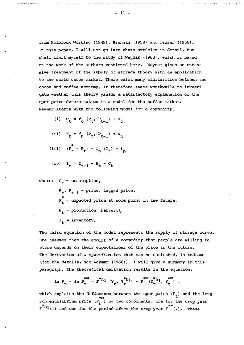
Weymar starts with the following model for a commodity.

( i ) C t = f c ( P t , P ^ ) + e c

( i i ) H t = fh ( P t , P t _ x ) + %

( i i i ) (P - P ) = f (I ) + e t t p t p

( i v ) \ - Vi + Ht - c t

where: C = consumption,

P , P = price, lagged price,

* P = expected price at some point in the future,

H = production (harvest),

I = inventory,

The third equation of the model represents the supply of storage curve.

One assumes that the amount of a commodity that people are willing to

store depends on their expectations of the price in the future.

The derivation of a specification that can be estimated, is tedious

(for the details, see Weymar (1968)). I will give a summary in this

paragraph. The theoretical derivation results in the equation:

In P. - In P. = F *oo *h *h *«• *h *«>

1 (Y,., Yfc *) - F (Y^ni, Y^ ) ,

which explains the difference between the spot price (P ) and the long

run equilibrium price (P ) by two components: one for the erop year •ht *°° F •••(.) and one for the period af ter the erop year F (.) . These

- 12 -

components depend on the current inventory ratio, Y = •— , the t

market's forecasted inventory ratio for the end of the erop year *hi *°°

h^, Y , and the expected long run equilibrium inventory ratio, Y .

Both the components have to be made operational.

Therefore, Weymar assumes that both the price and inventory ratios

approach their expected equilibrium values as t goes to infinity.

Weymar assumes initially that the equilibrium price equals the mean

of the deflated postwar prices. The monthly inventory ratio is known at

the beginning of the period, also known are the predictions concerning

the inventories at the end of the erop year and consumption during the

period, till the end of the erop year.

Weymar assumes that price expectations are a function of the expected

storage ratio and calls this the short run supply of storage function.

This function is assumed to be of the following form

,*h+l *h *h = b, + b„ In Y , where P = expected price at

horizon interval h; *h Y = inventory ratio expected

at horizon interval h.

In Weymar's study the time unit h is one month. The expected price change

from the present to the end of the erop year (h ) can be written as

*h . (bi + b2 ln Yt >

or ht" 1 *h

b h + I ln Y r h=0 c

where h is defined as

h = 12 in the final erop month

= 11 in one month before the final erop month etc.

I follow Weymar's study in which monthly data are used, but that is not

a loss of the generality, this theory can also be used for quarterly data.

- 13 -

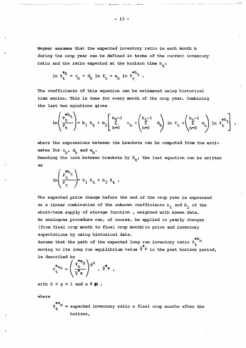
Weymar assumes that the expected inventory ratio in each month h

during the erop year can be defined in terms of the current inventory

ratio and the ratio expected at the horizon time h :

*h *n4-

ln Y = a + cL In Y + e In Y t .

The coefficients óf this equation can be estimated using historical

time series. This is done for every month of the erop year. Combining

the last two equations gives

*h.

l n l ! t _ , = b i h t + b 2 h t - i z h=0

where the expressions between the brackets can be computed from the esti-

mates for c, , d, and e, .

Denoting the term between brackets by Z , the last equation can be written

as

The expected price change before the end of the erop year is expressed

as a linear combination of the unknown coefficients b. and b„ of the

short-term supply of storage function , weighted with known data.

An analogous procedure can, of course, be applied in yearly changes

(from final erop month to final erop month) in price and inventory

expectations by using historical data. *s

Assume that the path of the expected long run inventory ratio Y n

_* *-moving to its long run equilibrium value Y s in the post horizon period,

is described by

with 0 < g < 1 and n G (H ,

where

*s Y n = expected inventory ratio n final erop months after the

horizon,

- 14 -

*s Y u = expected inventory ratio at the horizon,, _*s Y = expected equilibrium final erop month inventory ratio,

* g = parameter indicating the rapidity of Y 's approach towards

equilibrium»

After some substitutions of relationships given above, the equation to

be estimated can be written as

b., is a function of b„ and g.

P is the postwar average real spot price.

Weymar obtained good estimation results for this equation', when applied

to the cocoa market. Because of the similarities excisting between the

cocoa and coffee market, the supply of storage theory is a candidate

for explaining the spot price of coffee also.

The second subject of this paragraph concerns price relationships among

spot, futures and expected spot prices. Much research has been done

• on this subject. Some articles are briefly discussed in this paper.

The choice has been made with regard to the relevance of the hypotheses

for my model of the coffee market.

I will give some of the contributions in these articles with respect to

commodity prices in the spot and futures market, which illustrate diffe­

rent aspects of commodity market analyses. I make the following distinction.

- The forecasting properties of the futures prices for the

spot market prices.

- Hedging.

Let me start with the forecasting properties of the futures prices.

In the study of the futures market, Tomek and Gray (1970) concentrate on

the following relationship

P = a + b P£ , c f

with P = cash price at harvest time,

P = spring time futures price for end of the erop year.

- 15 -

The futuresprice is defined as a self-fulfilling forecast of the

cash price if for each year P = Pf. This hypothesis can be tested

for a commodity, by estimating the regression relationship between

the cash price and the prior futures price and testing whether the

intercept is zero and the slope is unity. Tomek and Gray have carried

out this test for commodities that are storable and those that are not.

They found substantial differences between these two kinds of commo­

dities. The hypothesis, a = 0 and b = 1, was not pejected for storable

commodities (corn, soybeans), for non-storable commodities (potatoes),

it was rejected. The distance between the futures and spot quotations

was 8 or 9 months.

This hypothesis is further elaborated by Kofi (1973) who uses the same

framework for analysing the reliability of futures quotations as pre-

dictors of spot prices. Just as Tomek and Gray, he carries out some tests,

using monthly data in the form of closing prices on the last trading day

of each month. He has computed regressions for the equation P^ = ot + 3-̂ ,+ £•

with P = cash price at harvest time,

P„ = previous futures quotations for harvest time contract. For coffee

the September contract is used.

e, = a random disturbance term. h

A difference from the study of Tomek and Gray is the variable distance be­

tween futures and spot quotations. The results for coffee over the*sample

period 1953-1969 are summarized in table 1 and figure 1, for different

distances between futures and spot quotations. 2

Kofi explains the decrease in r after eight months (deviation of the ex-

pected pattern) by the impact of the coffee agreement on the coffee prices.

- 16 -

distance A

a Ê 1

2 r

10 months -5.99 (11.06)

1.27 (.24)

.79

8 months 1.44 (7.05)

1.03 (.15)

.88

6 months 17.73 (7.40)

.66 (.14)

.75

2 months 13.03 (4.46

.74 (.08)

.92

1 month -5.73 (3.78)

1.14 (.07)

.97

Table 1: Estimation results of relationships between spot and futures prices, with Standard errors in parentheses

distance in months between futures quotations and 'contract -end

Fig.1: Predictine reliability of a coffee futures contract

- 17 -

The relationship between spot and futures price is also studied

by Danthine (1978). He emphasizes the informative role of futures

prices. For that reason he investigates the relationship between

spot and futures prices. Danthine (1978) analyses futures markets

as: "A place where hedgers compensate speculators for sharing the

risks inherent to their productive activity and shows that this

asymetry between economie agents reveals to futures price as a

biased estimate of the spot price and, in its own right, can gene-

rate speculative tradings".

I will now mention some studies with respect to hedging. A commo-

dity trader will hedge his inventory or demand if he wants to

eliminate the risk of sustaining a loss, caused by price changes.

The explanation of the shifting of risk is an important subject in

the futures trading literature. E.g. the analysis of the risk premium

required on a futures contract, as is done by Dusak (1973). Black

(1976) demonstrates that the futures market is not unique in its

ability to shift risk, but it is unique in the guidance of producers

and distributors concerning the values of forward contracts and

options in terms of the futures price and other variables.

Another aspect of futures trading is analysed by Rolfo (1980). In

his model he determines the optimal hedging percentage for cocoa

producers. Traditionally, speculation has not been taken into ac­

count and a complete hedge is therefore recommended. But uncertainty

about the agricultural production cannot be hedged in a futures mar­

ket.

Rolfo shows that; "Limited usage of the futures market may be superior

to a fuil short hedge of expected output, for producing countries when

there is production variability". This conclusion is not of direct

interest for the specification of the model in this paper, because

futures prices are not included in the model at this stage of the

project. It might be an interesting hypothesis which can be separately

tested later on.

The third mentioned subject for a discussion in this paragraph is the

efficiency of the spot and futures market. The efficiënt market

hypothesis is a well-known research topic in the financial literature,

and to a smaller extent in the literature with regard to commodity

- 18 -

prices. The literature on market efficiency is voluminous. I

will not try to give a complete survey here of the literature,

but I will discuss a few articles illustrating some important

aspects .

A market is called an efficiënt market if prices fully reflect

the available Information about the market» Fama (1970) gives

a detailed review of the theoretical and empirical research that

has been done on the efficiënt market model for capital markets.

He distinguishes three forms of market efficiency; weak form,

semi-strong form and strong form. In the weak form, the Informa­

tion used to determine market prices consists of historical prices

only. The semi-strong form concerns whether prices efficiently

adjust to public available information. The strong form concerns

whether groups of market participants exist which have monopolis-

tic access to information relevant for price formation. Most of

the hypotheses that have been tested concern the weak form market

efficiency. In that case the tests are concerned with the question

whether the prices follow a martingale. This is done by testing

whether price changes have been generated by a white noise prócess

or not.

Applications to commodity markets are given in Smidt (1965): soybean

futures prices, Stevenson and Bear (1970): corn and soybean futures

prices, and Praetz (1975): wool futures prices, Leuthold (1972) has

done a study with regard to the live cattle futures market. In all

these studies the investigators test whether price changes are

serially uncorrelated. With respect to the hypothesis of serially

uncorrelated price changes, it is important to mention the study

of Danthine (1977) who shows that in an efficiënt commodity marketf

changes in spot prices need not necessarily behave like a white

noise process. This is caused by specific features inherent in commodity

markets and so clearly distinct from capital markets. In Danthine's

model the market uncertainty is the demand for the commodity, while

in the coffee economy the uncertainty is the production (the yearly

erop). This aspect has to be taken into account when Danthine's

theory is applied to the coffee market.

- 19 -

It is certainly useful to mention that some of the articles dis-

cussed in this paragraph are reprinted in Goss and Yamey (1976).

Lastly I will discuss the use of commodity models for policy pur­

poses.

One of the most important policy purposes for a commodity markët

is to stabilize prices at a level acceptable to producing and

importing countries. Examples are the various commodity agreements

between producing and importing countries, as e.g. for wheat, coffee,

cacoa, sugar, tin. Also the efforts of UNCTAD to start a common fund

for raw materials have the same objective; see e.g. Barents (1980).

A review and appraisal of commodity price stabilization models is

given by Labys (1980). Most of these models use commodity buffer

stock policies. Here I will give a brief summary of Labys' article,

because many aspects of these types of models have been treated by

him.

Labys distinguishes the following three types of models.

1. Simple supply and demand relationships, which make it possible

to derive the expected gain to producers and consumers.

2. Empirical models with the same framework as under 1, but with

some variations dependent on the objective, showing differences

between stabilized and non-stabilized markets concerning income

effects and welfare gains.

3. Econometrie models with four basic equations: a demand supply and

price equation together with a stock identity where the buffer

stock variable is crucial to the price stabilization analysis.

His conclusion is: "None of the studies examined has overcome the

myriad of problems that analysts have pointed out as essential for

assessing the welfare outcomes of price stabilization schemes. As

a consequence, stabilization analyses for similar commodities have

produced conflicting results regarding predicted welfare outcome".

Because several studies have diverse results, Labys gives a number

of recommendations which could help to improve price stabilization

models. In short his recommendations are:

- Firstly, Labys mentions some studies with a greater number of com­

modities involved. By interrelating the corresponding commodity

models, multi commodity models are constructed. As to how far this

approach yields better results may be concluded after the recent

- 20 -

literature on this topic has been studied. Possibilities for

applying this idea to the coffee market seem to exist. E.g.

in my former analysis of daily prices it has been noticed that

prices of coffee, cocoa and tea are clearly correlated. At pre­

sent, it is hot my intention to construct a multicommodity model.

- More attention has to be given to the functional specification of

the econometrie relationships.

- The necessity of specifying the nature of private as well as

public stockholding in a commodity market, including interactions

between the two, is important.

- Attention for the dynamics of commodity market adjustments by

using e.g. spectral techniques to determine the underlying gene-

rating processes of price and inventory variables. Such an analysis

might improve the formulation of a dynamic buffer stock mechanism

in which price variance and trends are interrelated. It is our ex-

perience too, that the use of spectral techniques can help to im­

prove the specification of a model by better understanding of the

dynamics of the variables; see Vogelvang (1980).

- He recommends also stochastic simulation methods because

the'laistorical record is usually so short that it tells us little

of the future". Partial stabilization schemes can also be investi-

gated in this manner. Stochastic methods can help in learning how

the form of disturbances affects the outcome of stabilization ana­

lysis. This might be done for example by including shocks reflec-

ting uncertainty regarding climate, or by including probability

distributions associated wi'th different variables.

In Labys' opinion, more realistic results with stabilization models

could be obtained, when analysts take account of these recommendations.

In this paragraph many studies of commodity markets, theoretical and

empirical, have been discussed. In summary, some of the links between

these studies and a model for the coffee market are mentioned.

We reviewed existing econometrie research into the coffeemarket,

with the intention to show their features of price relationships,

and to place this project within the context of the literature.

Elements useful for our model have been found.

The supply of storage theory can be applied to the coffee market to

provide an equation for the price determination. The studies concerning

- 21 -

price relationships among spot and futures prices, and the

efficiënt market theory might be of use for an equation explaining

price expectations.

A second question to be analysed for the coffee market is to what

extent the ICA's have stabilized the market, as price stabilization

is one of the objectives of the I.C.A. Article 1 sub 1 and 2 of the

ICA-'76 reads as:

"The objectives of this Agreement are:

(1) to achieve a reasonable balance between world supply and demand

on a basis which will assure adequate supplies of coffee at fair

prices to consumers and markets for coffee at remunerative prices

to producers and which will be conducive to long-term equilibrium

between production and consumption;

(2) to avoid excessive fluctutuations in the levels of world supplies,

stocks and prices which are harmful to both producers and consumers;"

In Barents (1980) opinion, the ability of agreements to control the in­

ternational trade is very limited for raw materials as well as for cof­

fee; this we will investigate.

3» A model for the world coffee market

3.1 Introduction

In this paragraph a guarterly model for the coffee market will be

specified and its equations will be discussed. As the shortest time

interval, for which most of the variables of the model are available,

is per quarter, we shall use quarterly data. Quarterly data are expec-

ted to be more informative on the mechanism of price formation in the

coffee market than e.g. annual data.

In this section a flow diagram of the world coffee market is given

with a short explanation. The flow diagram forms the basis for the

specification of the model equations in section 3.2.

The model, as presented in 3.2, has to be seen as a general basic spe­

cification. For the equations of individual countries or regions, the

functional form of the equations and the explanatory variables may be

different. Data constraints will also influence the specification.

- 22 -

For instance, for the U.S.A., detailed information on imports and

consumption is available, while for East Europe and the U.S.S.R.

the data are scarce. The degree of aggregatioh of the model is

discussed at the beginning of section 3*2*

The equations of the model are discussed in detail in section 3.3.

A brief description of available data (available at this moment) is

given in section 3.4.

First we shall start with a flow diagram. Assumptions concerning the

causal relationships among variables of a model for the world coffee

market are represented by the arrows in figute 2, which gives a gene-

ral scheme.

production estimates

exogenous production influences

weather new cultivation techniques new planting or uprooting national or internat ional policies concer­ning the production or trade

expected spotprice

lagged spotprices

international agreement

inventories in prod.countries

retail price imp.countries

imports

inventories import.countries

^consumption

7 exogenou s demand influences

Fig. 2: A flow chart for the world coffee market

- 23 -

Some of the arrows deserve a short explanation. The influence of

the ICA on the spot price comes into operation when the spot price

is outside a price range during a number of days. The quota-system

then acts until the price is in the price range again (see I.C.O.

(1976) art.38). Production estimates are made quarterly by the United

States Department of Agriculture (USDA) and published in their coffee

information sheet. Also the Instituto Brasilerio do Café (IBC.) fur-

nishes production estimates. Concerning the exogenous production in-

fluences, we can mention that, at present, new cultivation techniques

are applied particularly in Columbia and result in a higher yield.

All the Latin American coffee producing countries have national coffee

bureaus, and these bureaus also try to control the coffee price by

means of export tax manipulation or by minimum registration prices.

Most of these bureaus are governed by the countries' ministry of

finance. New planting or uprooting plans are also developed by those

bureaus. Another channel through which producing countries today try

to affect the coffee price, is by operations on the New York Coffee

& Sugar Exchange. The producing countries, united in "the Bogota Group",

try to stabilize the coffee price at a high level by trading on this

Exchange. The Bogota Group consists of the following countries:

Brazil, Columbia, Costa Rica, El Salvador, Guatemala, Honduras, Mexico

and Venezuela. Sometimes Ivory Coast attends meetings of the Bogota

Group as an observer. As a reaction to the existence of the Bogota

Group, no further U.S. congressional action regarding I.C.A. imple-

menting legislation is expected. This is not the first time in the

coffee history, that producing countries act together in the market.

Exogenous demand influences are e.g. changes in consumption habits,

trends and prices of substitutes for coffee, like soft drinks and tea.

Obviously some of the relationships represented by the arrows, are

explained in the studies described in the former paragraph. For in-

stance, the relationship between production and spot price, between

spot and futures price, and aspects of the demand for coffee.

- 24 -

3.2 The specification of the model

In this paragraph I will give a general specification of the model.

A classification of importing and exporting countries is first dis-

cussed.

In appendix A, a survey is given of the exports and imports of the

member countries of the I.C.O. The figures ihdicate the impor-

tance of different countries with respect to their participation in

the coffee market. Important countries will be included seperately,

smaller countries will be grouped.

The producing countries will be distinguished according to the four

main types of coffee%

Columbian Milds

A. Colümbia

B. Kenya and Tanzania

Other Milds

C. One group of all countries

Unwashed Arabicas

D. Brazil

E. The other countries

Rob us tas

F. One group of all countries.

The importing countries can be grouped according to their similari-

ties in consumption habits, except for VI. At present, I propose the

following grouping:

I U.S.A.

II British Commonwealth and Ireland

United Kingdom, Ireland, Canada, Australia, New Zealand

III Scandinavia

Sweden, Denmark, Norway, Finland.

IV A number of Western European countries

West Germany, France, Netherlands, Italy, Belgium and

Luxembourg, Switzerland, Austria, Spain

V Japan

VI Non-member countries of the I.C.O.

- 25 -

From the tables in appendix A it is seen that exports to desti-

nations other than importing raerabers, amount to 5,669,000 bags

averaged over the years 1974-1978, while the average imports from

non-members for the same period equals 478,000 bags. Therefore,

non-member countries will be separately included in the model as

an importing group, which will not be treated in the same way as

the other importing groups, because this group is very heterogeneous

The equations of the model will now be presented. The following

indices are used:

coffee type , k € {1,.. , 4 } , 1

2

3

4

Columbian Milds

Other Milds

Unwashed Arabicas

Robustas

i : importing country ,

i € {!,.. ,6} , 1 corresponds to I

2 corresponds to II

etc.

producing country,

P e {i,..,6} , 1 corresponds to A

2 corresponds to B

etc.

An exogenous variable is denoted by an asterik as the last charac-

ter of its abbreviated name. The same symbol f is used in all the

equations, to indicate a functional relationship between variables.

World market prices

(la - ld) F* = f(P^ , Pk' , EPk, Qk* , INVk , EXPk)

k,k'€.{!,..,4} , k / k'

[2a - 2d) EP = f(.) k € {1,..,4}

1 1 1 2 3 4 (3) CDP = j (j (PX+PZ) + PJ + P*)

(4) ECDP = o" (j (EP + EP2) + EP + EP4)

- 26 -

Producing countries

(5a - 5f) EXP9 = f(Pk, EPk, O15*) P e {i,..,6}

(6a - 6f) INVP = INV^1 + PRODP* - EXpP p €. {1,..,6}

Importlng countries

(7a - 7f) IMP1 = f(INV1, CDP, Q1*, ECDP) i £ {1,..,5}

(8a - 8f) CONSX = f(CDP, PR1, TCI1*, exogenous demand influences)

i £ {1,..5}

(9a - 9f) PR1 = f(CDP_ , TAX*, MARK-UP*) i G {1,..5}

(10a - lOf) INV1 = INV1 + IMP1 - REEXP1* - CONS1

i G {lr..5}

Other identities

(11a - lid) INV = T INVP if country p produces coffee type k

k G {1, ...,4}

P

(12a - 12d) EXP = 2T EXPP if country p produces coffee type k

k G {1, ..., 4}

6 r> 6 i (13) I, EXPP = .1, IMP

p=l i=l

The following notation has been used

Je

EP

CDP

ECDP

PR1

PR0DP*

Qk*

QP*

Q1*

EKP*

EXP1'

spot price of coffee type k on the New York market (ICO-indicator)

expected spot price of coffee type k for some future point of time

composite daily indicator price, 1968 agreement

expected composite daily indicator price

retail price in country i

production in country p

export quota's of coffee type k

export quota's of producing country p

indication, that quota's are effective, for importing countries, as will be outlined in the next section

exports from country p to all destinations

total exports of coffee type k, from producing countries, to all destinations

27

IMP : imports of country i from all sourees

REEXP * : reexports from country i to all desti nations

INV , INV : inventory in country p or i

INV

CONS1

TCI1*

k total inventories of coffee type k, held by producers consumption in country i

total consumption index of country i

Summarized, the model exists of six structural equations, two defini-

tion equations and five identities, in its general specification. In

its (dis)aggregated form we have 51 equations. The 51 endogenous

variables are:

Pk, EPk, INVk, EXPk k e {1,..,4}

PR1, IMP1, INV1, CONS1 i e {1,..,5}

EXP^ INVP p £ {1,..,6}

CDP, ECDP and IMP .

The 31 exogenous variables are:

Qk* k € {1,..,4}

REEXP1*, TCI1*, Q1* i £ {1,..,5}

PRODP*, P^* p € {1,..,6}

The prices are measured in dollar cents per pound, the quantities

like exports, imports, inventories, quota's, are expressed in bags

of 60 kg, and consumption in gram per capita.

Time lags have been specified for some prices and in the identities.

The inclusion of time lags for other variables has been Ieft open.

- 28 -

3.3 Discussion of the equations of the model

We go on in this section with a detailed discussion of the model.

Production is assumed to be predetermined. This assumption is quite

natural for a quarterly model. Production is influenced by policy

decisions, like new planting, but it takes several years before the

erop is affected. A time-lag of five or more years can be expected.

It is possible to consider equation (1) as the solution for p of the k k

market clearing condition EXP = IMP , which cannot be explicitly in-r

cluded in the model because IMP is not observed. Therefore equation

(1) explains the spot price of coffee type k by means of the variables P i

determining supply, EXP , and demand, IMP .

When specifying equation (1) for one type of coffee, it might be neces-

sary to include one or more prices of other coffee types. But this is

only meaningful after knowledge has been obtained about price leader­

ship of one or more types of coffee. Bacha (1968) specifies e.g. the

Robusta price as an explanatory variable for the price of Milds (see

section 2.2). But if a price leader is present in the coffee market,

it will be the price of Unwashed Arabicas ar Columbian Milds, as Ro­

busta is an inferior type of coffee compared with these two.

A causality in the other direction, that is also done by Bacha, seems

appropriate.

Data on quotas do exist, but just as knowledge of the practice of the

ICA, it is still missing at this moment. Both are necessary for the

model.

The coherence between quota's, exports and imports has to be investi-

gated when data on quota's and the quota system has been made availa-s-

ble.

The supply of storage theory gives also an equation for the spot pri­

ces, as was outlined in the former paragraph. This can be an alterna-

tive rationale for a spot price equation.

Equation (2), the determination of the expected spot price, has been

left open so far. I shall discuss at first the other equations of the

model and then return to equation (2) for a comprehensive discussion

of possibilities for determining these price expectations.

Equation (3) is a definition. The composite daily indicator price is

computed in that way according to the 1968 coffee agreement. Accor-

ding to the 1976 agreement, the CDP is only the mean of the price of

Robustas and other Milds. Therefore, an indicator for the "world mar-

- 29 -

ket price" is better obtained by using the CDP-1968.

Equation (4) concerns the expected world market price and is com-

puted in the same way as the CDP, but now from the expected spot-

prices determined by equation (2).

For the producing countries an export equation (5) and an indenti-

ty determining inventories (6) are specified. In this identity, a

bufferstock variable can be inserted, which will be necessary when

policy simulations will be carried out with the model.

The demand for coffee in importing countries consists of the imports (7)

and the consumer demand (8). The specification of these equations re-

fer to the studies discussed in the former paragraph. It seems appro-

priate to include the world market price and the retail price in the

consumption equation, as consumers will use the world market price

as an indication for the future retail price. The exogenons influen-r

ces in the consumption equation are variables like trends, prices of

substitutes for coffee. Q x, in the import equation, denotes that

quota's are effective, and may be specified as a dummy variable. The

rationale for the inclusion of this variable is article 45 of the

I.CA.-1976: "To prevent non-member countries from increasing their

exports at the expense of exporting Members, each Member shall, when-

ever quota's are in effect, limit its annual imports of coffee from

non-member countries ".

Another modification for various equations, might be the specification

of net-imports instead of imports and re-exports, as it is not obvious

that re-export is a relevant variable for the price formation of cof­

fee. This last aspect is an important criterion for the model as sta-

ted at the beginning of this paper.

The major variable in explaining the retail price in equation (9) is

the lagged composite daily price. The retail price is expected to

follow the development of the coffee price on the world market. In

Vogelvang (1980) a correlation coëfficiënt of .65 has been found be-

tween the Dutch retail price of coffee and the CDP with a lag of 3

months. This was computed from monthly data in the sample period

1970-1979 (March).

Equation (10) is an identity for the inventories in importing coun­

tries.

- 30 -

The equations for the importing countries have been indicated for

the first five groups of importing countries. The group of non-

tnember countries are omitted in this block. This is a rather di­

verse group of countries: USSR, East European countries, Greece,

Asian countries, non-producing African and Latin American coun­

tries. Therefore, it is not meaningful to specify and estimate

structural equations for this whole group.

The imports to these countries are determined through the identity

(13), IMP has therefore been mentioned seperately in the list of

endogenous variables.

Equations (11) and (12) determine the total inventories in, and

exports from exporting countries for one type of coffee.

Equation (13) keeps total imports from all sources in balance with

total exports to all destinations and determine IMP as was outli-

ned before.

Lastly, I shall discuss some possibilities for the determination of

expected spot prices,

Different hypotheses can be postulated as to how price expectations

are formed. Here I assume that producers and importing roasters form

their expectations in the same way using information on the (expected)

market circumstances. Also past prices will be relevant in some cir­

cumstances. Factors affecting the erop of coffee in producing coun-r

tries will dominate the formation of price expectations. Due to the

consumption habits, the demand for coffee by importing countries is

in fact a stable variable, as long as prices do not change too much.

Only in particular market circumstances, e.g. in case of large price

changes leading to high prices, will the demand factor become a less

stable factor.

Forecasts of the next erop influence the market. When disastrous cir­

cumstances arise in the production areas, e. g. many coffee plants

are destroyed by heavy frost, bad weather or plant diseases, fore­

casts for a period, longer than one year, can be made and will in­

fluence the market.

I will now describe some possible specifications for the formation

of price expectations on the spot market. Usually price expectations

are not observed, therefore we have to make assumptions about this

formation of price expectations,

#

- 31 -

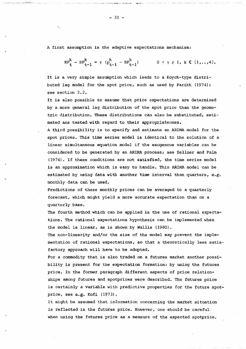
A first assumption is the adaptive expectations mechanism:

EP* - EP^_1 = Y (P^_j " EP^j) 0 < y ̂ 1, k £ {1,..,4}.

It is a very simple assumption which leads to a Koyck-type distri-

buted lag model for the spot price, such as used by Parikh (1974);

see section 2.2.

It is also possible to assume that price expectations are determined

by a more general lag distribution of the spot price than the geome­

trie distribution. These distributions can also be substituted, esti­

mated ans tested with regard to their appropriateness.

A third possibility is to specify and estimate an ARIMA model for the

spot prices. This time series model is identical to the solution of a

linear simultaneous equation model if the exogenous variables can be

considered to be generated by an ARIMA process; see Zellner and Palm

(1974). If these conditions are not satisfied, the time series model

is an approximation which is easy to handle. This ARIMA model can be

estimated by using data with another time interval than quarters, e.g.

monthly data can be used.

Predictions of these monthly prices can be averaged to a quarterly

forecast, which might yield a more accurate expectation than on a

quarterly base.

The fourth method which can be applied is the use of rational expecta­

tions. The rational expectations hypothesis can be implemented when

the model is linear, as is shown by Wallis (1980).

The non-linearity and/or the size of the model may prevent the imple-

mentation of rational expectations, so that a theoretically less satis-

factory approach will have to be adopted.

For a commodity that is also traded on a futures market another possi­

bility is present for the expectation formation: by using the futures

price. In the former paragraph different aspects of price relation-

ships among futures and spotprices were described. The futures price

is certainly a variable with predictive properties for the future spot-

price, see e.g. Kofi (1973).

It might be assumed that information concerning the market situation

is reflected in the futures price. However, one should be careful

when using the futures price as a measure of the expected spotprice.

- 32 -

As Danthine (1978) indicates: the futures price was stated as a

biased estimate of the spot price; see section 2.3.

At present, the choice of a specification of the expected spot

price will be provisionally left open.

So far, a description of the equations has been given of a basic

model for the world coffee market.

In the introduction of this paper, two objectivies of this study

have been mentioned: the explanation of price formation, and poli­

cy simulation. Both can be done with this model. The emphasis on

prices in this section underlines the first objective. For policy

purposes, different possibilities exist. At first, the quota varia­

ble, which has been inserted in three equations of the model, can

be used as a policy instrument to analyse the effects of I.C.O.-mea-

sures. Effects of consumer actions, such as boycotts, on the spot-

price go through equations (8), (10), (7), (13) and (1.2). Simulations

can be done by slightly modifying the model by the inclusion of a

policy variable in equation (8).

Producer actions like export limitations can be inserted in the model

in the same way by including a policy variable in equation (5). This can

also be done by making use of the buffer stocks in equation (6). The

spot price is influenced then through the identities (6) and (12).

Effects of futures trading by producing countries can be analysed by

means of including futures prices in equation (2).

I call the presented model a basic model as no distinction has been

made yet in the functional form of the equations for the different

regions of the coffee economy. On the basis of this concept, further

refining of the model will take place.

3.4 The data

In this section a short description of available data will be given.

All the data, necessary for the estimation of the model, has not been

collected yet, but their sources in which they are published are known,

see appendix B. For lack of availability, the Annual Coffee Statistics

of the Pan American Coffee Bureau have not yet been used. This Bureau,

which does not exist anymore, has published the Annual till 1975 and

furr\ished in those years the most complete quantity of data. Today,

this is done by the I.C.O. with regard to the statistical tables.

- 33 -

These four publications (and the Annual Coffee Statistics) are

the most important publications that provide coffee data.

The longest period for which the main variables are available

on a quarterly basis is from the 4th quarter of 1971 until the

4th quarter of 1979. It is very propable that earlier data can

also be obtained. When in the following description a sample pe­

riod is not mentioned, it concerns the periode 1971 to 1979

Similarly, when the source of data is not mentioned explicitly,

they are taken from the I.C.O.- bulletins.

Monthly prices of the four main types of coffee on the New York mar-

ket are available from 1947-1979. Retail prices are available for

most importing countries in national currency and $ct/lb since 1976 .

Export figures exist per exporting member to all destinations, just

asimport figures exist per importing member from all sources.

Inventories in importing countries are known at the end of each

quarter. Opening stocks of producing countries at the beginning of

the erop year are published.

For Brazil, monthly inventories are known from the Annual Report.

Consumption series for the importing countries are defined as the

disappearance. Disappearance is the net import of all forms of cof­

fee, adjusted for changes in visible inventories.

Production estimates are published quarterly by the U.S.D.A. Most of

them have still to be collected.

From this summary of the data exploration, it should be clear that

the objective stated in this paper can be realized, althou^i various

data still have to be collected.

- 34 -

4 Summary and conclusions

In this paper a quarterly econometrie model for the world coffee

market has been proposed. Two objectives have been formulated:

1. Analysis of the price formation of coffee on the world market,

and testing of specific hypotheses concerning the behaviour of

producers and consumers;

2. Simulations of the impact of different policies of the I.C.A and

the producing countries.

On behalf of the construction of an econometrie model for the world

coffee market a survey has been given of some existing coffee models

and of a number of studies on commodity market analysis with regard

to price formation. The model presented in this paper is designed for

a detailed analysis of the price formation of coffee and for short-

run policy simulations. An outline of the structure of the model has

been given. Many refinements, concerning the functional form and

dynamics of the model, and assumptions about the stochastic proper-

ties (disturbances) of the model, are still required. This will be

done in the next stage of the research, before a first version of the

model will be estimated.

- 35 -

Appendix A

table Al. Exports to all destinations by exporting member, grouped

by coffee type.

table A2. Imports from all sources by importing member.

Source: Quarterly Statistical Bulletin, I;C.O.

Table A.1

- 36 -

EXPORTS TO ALL DESTINATIONS: BY EXPORTSNG MEMBER 1975 TO 1979

(000 bags)

1975 1976 1977 1978 1979

1978 1979

Exporting Member 1975 1976 1977 1978 1979 IV I II III IV

TOTAL 57,874 58,522 46,921 55,815 62,263 15,076 16,222 16,964 14,656 14,422

Colombian Milds 10,132 8,530 7,616 11,262 13,257 3,366 3,840 3,094 3,165 3,157

Colombia 8,175 6,289 5,323 9,034 11,131 2,957 3,157 2,486 2,831 2,657 Kenya 1,104 1,262 1,534 1,415 1,279 291 363 328 250 338 Tanzania 853 979 759 813 847 118 320 280 84 162

Other Milds 15,723 16,475 14,578 15,804 19,346 3,692 5,680 5,352 3,863 4,453

Burundi 421 366 282 385 463 94 2 26 331 104 Costa Rica 1,274 1,091 1,187 1,412 1,625 375 608 336 244 438 Oominican Republic 531 700 738 459 726 108 140 133 81 372 Ecuador 1,072 1,531 923 1,638 1,418 319 296 246 497 380 El Salvador 3,062 2,666 3,015 2,347 3,390 407 1,143 1,347 484 416 Guatemala 2,158 2,142 2,173 2,204 2,582 711 848 741 257 735 Haiti 315 419 289 257 361 46 69 78 43 171 Honduras 812 722 .599 958 1,101 104 530 300 117 154 India 993 833 912 1,071 1,029 253 230 301 277 221 Jamaica 20 18 17 9 15 2 5 4 3 3 Malawi 1 3 2 3 6 - 1 - 3 2 Mexico 2,392 2,751 1,783 1,970 2,990 559 1,022 974 516 478 Nicaragua 674 802 802 887 923 166 330 367 64 161 Panama 26 25 19 39 48 7 15 11 5 18 Papua New Guinea 595 799 626 769 826 137 96 210 365 155 Peru 720 703 741 892 1,157 299 175 165 433 384 Rwanda 428 606 282 268 555 52 79 83 136 257 Venezuela 229 298 188 236 131 53 91 30 7 4

Unwashed Arabicas 15,712 16,921 11,025 13,886 13,602 4,783 2,981 3,820 3,151 3,651

Bolivia 86 78 78 92' 114 6 4 37 54 20 Brazil 14,604 15,602 10,083 12,551 12,010 4,628 2,623 3,215 2,751 3,421

Ethiopia 923 1,190 833 1,156 1,448 138 339 564 340 204 Paraguay 99 51 31 87 30 11 15 4 6 6

Robustas 16,307 16,596 13,702 14,863 16,058 3,235 3,721 4,698 4,477 3,161

Angola 2,665 1,395 1,039 1,297 963 335 186 283 208 286 Ghana 44 61 54 17 22 3 2 3 8 9 Guinea 55 17 33 11 33 0 0 4 8 21 Indonesia 2,168 2,106 2,515 3,460 3,607 935 696 1,571 693 648 Liberia 69 70 165 146 140 24 20 38 60 23 Nigeria 20 91 46 20 34 19 10 3 20 -0AMCAF (7,158) (8,791) (6,317) (6,622) (7,605) (1,077) (1,561) (2,202) (2,492) (1,349)

Benin 37 29 10 3 1 2 0 1 0 0 Cameroon ' 1,623 1,641 1,159 1,378 1,718 270 229 462 598 429 Central African Rep. 166 145 150 153 101 16 28 31 28 14 Congo 12 30 30 63 95 25 22 32 24 16 Gabon 2 4 3 3 6 - 1 2 1 1 Ivory Coast 4,096 • 5,547 4,021 4,093 4,620 526 1,030 1,376 1,681 533 Madagascar 1,089 1,216 844 823 899 219 220 256 127 296 Togo 133 179 100 106 165 19 31 42 33 60

Sierra Leone 106 53 153 92 222 0 97 104 17 4 Trinidad and Tobago 55 45 41 28 35 4 13 12 7 3 Uganda 2,943 2,552 2,200 1,895 2,371 585 860 273 635 602 Zaire 1,024 1,415 1,139 1,275 1,026 253 276 205 329 216

Green 55,797 55,728 44,728 53,021 58,835 14,159 15,484 16,074 13,777 13,500

(Procesaed) (2,077) (2,794) (2,193) (2,794) (3,428) (917) (738) (890) (878) (922)

Roasted 233 314 231 150 195 13 52 82 22 39 Soluble 1,844 2,479 1,957 2,608 3,233 904 686 808 856 883

To import ing Members 51,744 52,338 42,401 50,270 56,413 13,628 14,783 15,093 13,316 13,221

To other destinations 6,130 6,184 4,520 5,545 5,850 1,448 1,439 . 1,871 1,340 1,201

Brazil 14,604 15,602 10,083 12,551 12,010 4,628 2,623 3,215 2,751 3,421

Colombia 8,175 6,289 5,323 9,034 11,131 2,957 3,157 2,486 2,831 2,657

Other Arabicas 18,788 20,035 17,813 19,367 23,064 4,256 6,721 6,565 4,597 5,183

Robustas 16,307 16,596 13,702 14,863 16,058 3,235 3,721 4,698 4,477 3,161

Less than 500 bags

- 37 -

T a b l e A.2

IMPORTS F ROM ALL SOURCES: BY IMPORTING MBABER 1975 TO 1979

(000 bags)

1975 1976 1977 1978 1979

1978 1979

I m p o r t i n g Member 1975 1976 1977 1978 1979 IV i II I I I IV

TOTAL 57,528 59,607 49,318 54,877 62,849 15 ,556 15 ,239 16 ,672 15,565 15,374

U . S . A . 21,722 21,712 16,541 19,785 21,446 5 ,673 5 ,184 5 ,820 5,214 5,228

E . E . C . 22,741 23,551 20,762 22,957 26,482 6_ ,290 6_ ,394 6 ,804 6,796 6,490

B e l g i u m / L u x e m b o u r g 1,553 1,546 1,242 1,447 1,765 406 432 447 455 432

Denmark 1,119 1,103 871 1,003 1,006 282 254 226 267 258

F . R . o f Germany 6,344 6,658 6,516 6,924 8,147 1 ,989 1 ,789 2 ,084 2,098 2,176

F r a n c e 5,295 5,267 4,861 5,442 5,728 1 ,430 1 ,537 1 ,495 1,423 1,273

I r e l a n d 41 62 39 50 71 13 19 19 17 16

I t a l y 3,399 3,588 3,076 3,265 3,831 914 949 881 925 1,077

Netherlands 2,791 2,985 2,232 2,675 2,955 676 735 755 773 693

United Kingdom 2,199 2,342 1,925 2,151 2,979 580 679 897 838 565

Other Members 13,065 14,344 12,015 12,135 14,921 3 ,593 2 ,661 4 ,048 3,555 3,656

Aus tra l ia 442 533 449 446 612 135 123 143 180 165

Austria 620 666 513 612 751 144 186 170 221 174

Canada 1,778 1,702 1,433 1,693 1,793 482 424 479 478 412

Cyprus 25 28 22 26 37 y 4 13 <4 10 6 U

Finland 1,003 1,174 817 896 1,110 220 334 357 210 209

Hong Kong 293 300 211 61 92 22 13 21 17 41

Hungary 545 632 714 371 558 115 125 183 84 165

I sraë l 180 2/ 295 160 197 178 y 54 2/ 46 2/ 46 2 / 44 2 / 44 2 /

Japan 2,034 2,657 2,479 1,873 3,338 641 748 983 894 714

Ne» Zealand 90 94 66 97 117 27 18 29 27 42

Norway 648 689 552 683 693 201 179 148 186 180

Portugal 255 342 206 178 202 y 73 65 51 13 72 2 /

Spain 1,296 1,566 1,392 1,759 1,753 570 429 433 422 469

Sweden 1,931 2,038 1,218 1,585 1,728 476 400 442 370 517

Switzerland 1,151 1,017 951 886 989 245 256 302 207 224

Yugoslavi a 774 611 832 772 970 184 302 253 192 222

Green (Processed)

Roasted Soluble

53,389 54,637 44,735 50,084 56,386 14,186 13,848 14,851 (4 ,139) (4 ,970 ) (4 ,583 ) (4 ,793 ) (6 ,463 ) (1 ,370) (1 ,391) (1 ,821 )

977 1,110 1,134 1,132 1,512 238 262 496 3,137 3,818 3,393 3,572 4 ,838 1,103 1,093 1,301

13,784 13,903 (1 ,781) (1 ,471)

421 334 1,329 1,115

From

Export ing Hembers 53,843 Importing Members 3,236 Non-members 435 Unspecified or ig ins and designated t e r r i t o r i e s 14

55,371 3,657

552

27

45,949 2,994

364

11

51,246 58,558 3,040 3,735

578 535

14,465 927 161

14,320 814 102

15,461 1,093

115

14,436 948 172

14,341 880 146

13 21

y Includes es t imates provided by the Hember 2/ Estimated

- 38 -

Appendix B

Sources of data

1. Quarterly Statistical Bulletin on Coffee, published by the Inter­

national Coffee Organization (London), Vol. 1 (1977) - Vol. 3 (1979).

2. Coffee Annual, published by George Gordon Paton & Co., New York,

1974-1977.

3. Annual Report, published by the Nederlandse Vereniging voor de Koffie-

handel, Amsterdam, 1960-1976.

4. Foreign Agriculture Circular, Coffee, published by the U.S. Dept. of

Agriculture, Washington, 1977-1980 (irregular).

5. Annual Coffee Statistics, published by the Pan-American Coffee Bureau,

New York.

- 39 -

References

Arak, M. (1968): "The price responsiveness of Sao Paulo coffee growers", Food Research Institute Studies in Agricultural Economics, Trade and development, VIII, 211-223.

Bacha, E. (1968): An econometrie model for the world coffee market: the impact of Brazilian price policy, dissertation, Yale üniversity.

Barents, R. (1980): "Het gemeenschappelijk grondstoffenfonds", Econo­misch Statistische Berichten, 65, 893-899.

Black, F. (1976): "The pricing of commodity contracts", Journal of finan-cial economics, 3, 167-179.

Brennan, M.J. (1958): "The suppy of storage", American Economie Review, 47, 50-72.

Bucholz, H.E. (1964): Der Kaffeemarkt in Deutschland, Meisenheim am Glau, Verlag Anton Hain.

Danthine, J.-P. (1977): "Martingale, market efficiency and commodity pri-ces", European Economie Review, 10, 1-17.

Danthine, J.-P. (1978): "Information, futures prices, and stabilizing speculation", Journal of Economie Theory, 17, 79-98.

Dusak, K. (1973): "Futures trading and investor returns: an investigation of commodity market risk premiums", Journal of Political Economy, 81, 1387-1406.

Edwards, R. and A. Parikh (1976): "A stochastic policy simulation of the world coffee economy", American Journal of Agricultural Economics, 58, 152-160.

Fama, E.F. (1970): "Efficiënt capital markets: a review of theory and empirical work", The Journal of Finance, 25, 383-417.

Ford, D. (1977): Coffee supply, trade and demand: an econometrie analy-sis of the world market 1930-1969, dissertation, Üniversity of Pennsyl-vania.

Gelb, A.H. (1974): "Coffee prices and the Brazilian exchange rate", Ox­ford Economie Papers, 26, 104-119.

Gelb, A.H. (1977): "Optimal control and stabilization policy: An appli-cation to the coffee economy", Review of Economie Studies, 44, 95-109.

Gelb, A.H. (1979): "A spectral analysis of coffee market oscillations", International Economie Review, 20, 495-514.

Goss, B.A. and B.S. Yamey (eds) (1976): The economics of futures trading, Mac Millan.

International Coffee Organization (1976): International Coffee Agreement 1976, London.

- 40 -

Kofi, T.A. (1973): "A framework for comparing the efficiency of futures markets", American Journal of Agricultural Economics, 55, 584-594.

Labys, W.C. (1980): "Commodity price stabilization models: A review and appraisal", Journal of Policy Modeling, 2, 121-136.

Leuthold, R.M. (1972) : "Random walk and price trends: The live cattle fu­tures market", Journal of Finance, 27, 879-889.

Parikh, A. (1974): "A model of world coffee economy 1950-68", Applied Eco­nomics, 6, 23-43.

Parikh, A. (1979): "Estimation of supply functions for coffee", Applied Economics, 11, 43-54.

Praetz, P.D. (1975): "Testing the efficiënt markets theory on the Sidney Wool Futures Exchange", Australian Economie Papers, 14, 240-249.

Rolfo, J. (1980): "Optimal hedging under price and quantity uncertainty: the case of a cocoa producer", Journal of Political Economy, 88, 100-116.

Rourke, B.E. (1970): "Short-range forecasting of coffee production", Food Research Institute studies in Agricultural Economics, Trade, and Develop-ment, IX, 197-214.

Smidt, S. (1965): "A test of the serial independence of price changes in soybean futures", Food Research Institute Studies, 5, 117-136.

Stevenson, R.A. and R.M. Bear (1970): "Commodity futures: trends or ran­dom walks?", The Journal of Finance, 25, 65-81.

Telser, L,G. (1958): "Futures trading and the storage of cotton and wheat", Journal of Political Economy, 66, 233-255.

Tomek, W.G. and R.W. Gray (1970): "Temporal relationships among prices on commodity futures markets: their allocative and stabilizing roles", Ameri­can Journal of Agricultural Economics, 52,. 372-380.

Verdam, R. (1977): "De koffieïmporten in Engeland", werkstuk econometrie, Economische Fakulteit V.U.

Vogelvang, E. (1980): "A short term econometrie model for the consumer demand of roasted coffee in the Netherlands", Kwantitatieve Methoden, 1, 110-131.

Wallis, K.F. (1980): "Econometrie implications of the rational expecta-tions hypothesis", Econometrica, 48, 49-73.

Weymar, F.H. (1968): The dynamics of the world cocoa' market, Cambridge, The M.I.T. Press.

Wickens, M.R. and J. Greenfield (1969) : "The econometrics of agricultu­ral supply: an application to the world coffee market", The Review of Economics and Sbatistics, 55, 433-440.

- 41 -

Working, H. (1949): "The theory of the price of storage", American Economie Review, 31, 1254-1262.

Zellner, A. and F. Palm (1974): "Time series analysis and simutaneous equation econometrie models", Journal of Econometrics, 2, 17-54.

42 Serie Research 'Memoranda;

1977-1 L. Hordijk, P. Nijkamp,

1977-2

1978-1

P. Nijkamp,

J. Klaassen,

1978-2 P, Nijkamp, M.W. van Veenendaal,

1978-3 P. Nijkamp, J. Spronk,

1978-4 P. Nijkamp, P. Rietveld,

1978-5 P. Nijkamp,

1978-6 P. Nijkamp,

1978-7 P. Nijkamp,

1978-8 J.D.P. Kasper,

1978-9 H.J. Blommestein, P. Nijkamp, P. Rietveld,

1978-10 F. Palm and A. Zellner,

1978-11 J.H.T.H. Andriessen, P.A. Cornelis, H. van der Flier,

1978-12 W. van Lierop and

P. Nijkamp,

1978-13 R.J. Joseph,

1978-14 P. Nijkamp en W. van Veenendaal,

1979-1 A.A. Schreuder-Sunderman,

i;st imation of Spatiotemporal Models New directions via distributed lags and Markow schemes.

Gravity and entropy models: The state of the art,

Valuta problemen in de Jaarrekening.

Psychometrie scaling and preference methods in spatial analysis.

Interactive Multiple Goal Programming.

New Multi Objective Techniques in Physical Planning.

Decision Models for Planning against Stagnation.

A Theory of Displaced Ideals. An Analysis of Interdependent Decision via Non-Linear Multi-Objective Optimization.

Conflict Patterns and Compromise Solutions in Fuzzy Choice Theory. An Analysis and application.

De Bijdrage van Detailhandelsmarketing aan Maatschappelijke Welvaart en Welzijn.

A Multivariate Analysis of Spatial Inequa-lities.

Large Sample Estimation and Testing Proce­dures for Dynamic Equation Systems.

Participatie, Invloed, Satisfactie en Groepseffectiviteit. Een onderzoek bij deelnemers aan een bedrijfsspel.

A utility framework for interaction models for spatial processes.

Beschermingsconstructies in het huidige en komende vennootschapsrecht.

A multi-attribute analysis of spatial choice Behaviour.

Werknemers en Soc. Jaarverslag.

1979-2

Frans Blommaert en Hein Schreuder,

H. Schreuder,

1979-3 P. Nijkamp en P. Rietveld,

1979-4 J. Arntzen, G. Bornmalm-Jardelöw and P. Nijkamp,

1979-5 P. Nijkamp, A. Soffer

1979-6 drs. A.J. Mathot

1979-7 H. Blommestein, P. Nijkamp en W. van Veenendaal,

1979-8 H.J.Blommestein and F.C. Palm

De maatschappelijke verantwoordelijkheid van Ondernemingen.

Multilevel Multi-objective Models in a Multiregional System.

Duality, Segmentation and Dynamics on a Regional Labour Market.

Soft Multicriteria Decision Models for Urban Renewal Plans.

A Model of choosing a car with or without a credit.

Shopping Perceptions and preferences: A multi-dimensional Attractivenerss Analysis of Consumer and Entrepreneurial Attitudes. The Aggregate Demand for Money in the Netherlands-: a new look at a study of the Bank of the Netherlands.