a quantitative reasoning approach to algebra using inquiry

Numeracy Numeracy Advancing Education in Quantitative Literacy Advancing Education in Quantitative Literacy

Volume 10 Issue 2 Article 4

2017

A Quantitative Reasoning Approach to Algebra Using Inquiry-A Quantitative Reasoning Approach to Algebra Using Inquiry-

Based Learning Based Learning

Victor I. Piercey Ferris State University, [email protected]

Follow this and additional works at: https://scholarcommons.usf.edu/numeracy

Part of the Science and Mathematics Education Commons

Recommended Citation Recommended Citation Piercey, Victor I.. "A Quantitative Reasoning Approach to Algebra Using Inquiry-Based Learning." Numeracy 10, Iss. 2 (2017): Article 4. DOI: http://doi.org/10.5038/1936-4660.10.2.4

Authors retain copyright of their material under a Creative Commons Non-Commercial Attribution 4.0 License.

http://scholarcommons.usf.edu/

http://scholarcommons.usf.edu/

https://scholarcommons.usf.edu/numeracy

https://scholarcommons.usf.edu/numeracy/vol10

https://scholarcommons.usf.edu/numeracy/vol10/iss2

https://scholarcommons.usf.edu/numeracy/vol10/iss2/art4

https://scholarcommons.usf.edu/numeracy?utm_source=scholarcommons.usf.edu%2Fnumeracy%2Fvol10%2Fiss2%2Fart4&utm_medium=PDF&utm_campaign=PDFCoverPages

http://network.bepress.com/hgg/discipline/800?utm_source=scholarcommons.usf.edu%2Fnumeracy%2Fvol10%2Fiss2%2Fart4&utm_medium=PDF&utm_campaign=PDFCoverPages

http://creativecommons.org/licenses/by-nc/4.0/

A Quantitative Reasoning Approach to Algebra Using Inquiry-Based Learning A Quantitative Reasoning Approach to Algebra Using Inquiry-Based Learning

Abstract Abstract In this paper, I share a hybrid quantitative reasoning/algebra two-course sequence that challenges the common assumption that quantitative literacy and reasoning are less rigorous mathematics alternatives to algebra and illustrates that a quantitative reasoning framework can be used to teach traditional algebra. The presentation is made in two parts. In the first part, which is somewhat philosophical and theoretical, I explain my personal perspective of what I mean by “algebra” and “doing algebra.” I contend that algebra is a form of communication whose value is precision, which allows us to perform algebraic manipulations in the form of simplification and solving moves. A quantitative reasoning approach to traditional algebraic manipulations rests on intentional and purposeful use of simplification and solving moves within contextual situations. In part 2, I describe a 6-week instructional module intended for undergraduate business students that was delivered to students who had placed into beginning algebra. The perspective described in part 1 heavily informed the design of this module. The course materials, which involve the use of Excel in multiple authentic contexts, are built around the use of inquiry-based learning. Upon completion of this module, the percentage of students who successfully complete model problems in an assessment is in the same range as surveyed students in precalculus and calculus, approximately two “grade levels” ahead of their placement.

Keywords Keywords numeracy, quantitative literacy, quantitative reasoning, education, algebra, algebraic manipulations, business education, mathematics education, inquiry-based learning, spreadsheets in education

Creative Commons License Creative Commons License

This work is licensed under a Creative Commons Attribution-Noncommercial 4.0 License

Cover Page Footnote Cover Page Footnote Victor Piercey received his Ph.D in mathematics from the University of Arizona in 2012. Dr. Piercey also holds a B.A. in Humanities from Michigan State University, a law degree from Columbia University with a certificate in international and comparative law, and a M.S. in Mathematics from Michigan State University. He practiced law in the New York office of Weil, Gotshal, & Manges LLP for two years before returning to Michigan for a career in Mathematics. Dr. Piercey began working as an assistant professor in the mathematics department at Ferris State University in the fall of 2012 and is currently an associate professor. He is interested in using his legal experience to enhance his mathematics instruction and provide students with transformative experiences. His current project is an inquiry-based sequence of courses entitled Quantitative Reasoning for Professionals. Some sections of this course are linked with sections of freshman writing courses.

This article is available in Numeracy: https://scholarcommons.usf.edu/numeracy/vol10/iss2/art4

https://creativecommons.org/licenses/by-nc/4.0/legalcode



https://scholarcommons.usf.edu/numeracy/vol10/iss2/art4

Introduction

Quantitative literacy and quantitative reasoning courses are often considered “less- rigorous” alternatives to algebra. For example, Hamman and Kung (2017) express a concern that quantitative literacy courses are used in place of algebra, and this practice may unintentionally impede equitable access to high-quality mathematics. Their commentary is based in part on Moses and Cobb (2002), in which access to quality instruction in algebra is cast as a civil right. While Hamman and Kung (2017) are careful to point out that quantitative literacy and algebra need not and should not be disjoint, their empirical observations illustrate a common, unstated assumption in the community – that quantitative literacy/quantitative reasoning is the “non-algebra” curricular option. This assumption needs to be challenged. For example, many quantitative reasoning textbooks include topics involving linear and exponential modeling (e.g., Bennett and Briggs 2014). Steen (2001) stated that quantitative literacy and reasoning required knowing “more than formulas and equations,” an indication that we are actually talking about a larger, and deeper, domain of thinking. Gaze (2014) proposes that quantitative reasoning, with an emphasis on proportional reasoning and modeling, should enhance algebraic reasoning.

On the other hand, numeracy, quantitative literacy, and quantitative reasoning are often characterized by a focus on numerical, not algebraic, information. Steen (1999) himself emphasized understanding numerical information that surrounds us in what he called a “data-drenched society.” Zillman et al. (2009) place the role of numerical data presented in the news at the center of quantitative literacy. The Association of American Colleges and Universities (2010) in its VALUE rubric describes quantitative literacy as “an at-homeness” with numbers. Others, such as Geiger et al. (2015) consider quantitative literacy to be essential to citizenship and participation in a democracy.

In the following, we ask what the proper relationship is between quantitative reasoning and algebra. More specifically, we ask how algebra and quantitative reasoning may overlap, what a curricular module implementing this overlap could look like, and what impact such a curricular module may have on students’ basic algebraic skills. Throughout, we should observe that facility with numerical information and algebra need not be mutually exclusive. In fact, these skills can support one another, as Gaze (2014) envisions.

As an illustration of what a quantitative reasoning approach to algebra could look like, compare the following two problems:

Problem 1: Solve 𝐶 = 1 − 𝐴𝑎 for A.

1

Piercey: A QR Approach to Algebra

Published by Scholar Commons, 2017

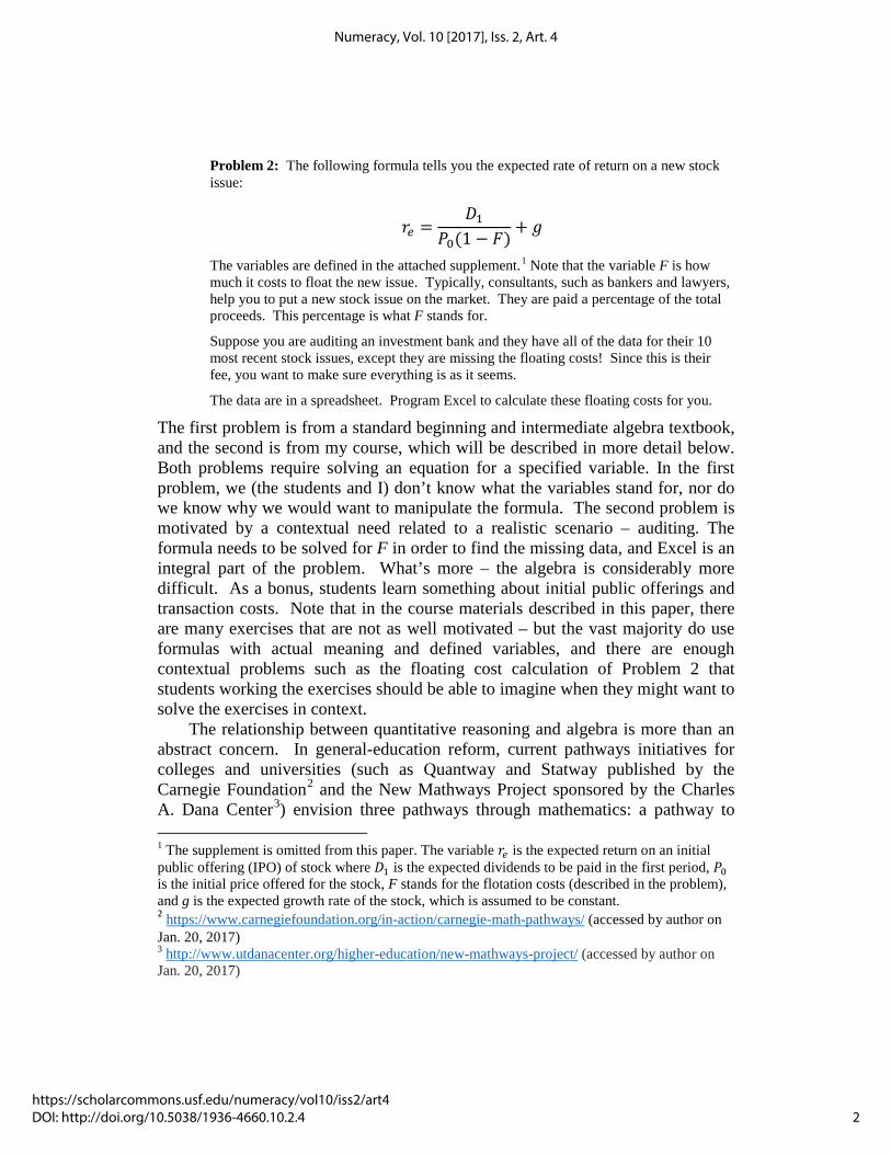
Problem 2: The following formula tells you the expected rate of return on a new stock issue:

𝑟𝑒 =𝐷1

𝑃0(1 − 𝐹)+ 𝑔

The variables are defined in the attached supplement.1 Note that the variable F is how much it costs to float the new issue. Typically, consultants, such as bankers and lawyers, help you to put a new stock issue on the market. They are paid a percentage of the total proceeds. This percentage is what F stands for.

Suppose you are auditing an investment bank and they have all of the data for their 10 most recent stock issues, except they are missing the floating costs! Since this is their fee, you want to make sure everything is as it seems.

The data are in a spreadsheet. Program Excel to calculate these floating costs for you.

The first problem is from a standard beginning and intermediate algebra textbook, and the second is from my course, which will be described in more detail below. Both problems require solving an equation for a specified variable. In the first problem, we (the students and I) don’t know what the variables stand for, nor do we know why we would want to manipulate the formula. The second problem is motivated by a contextual need related to a realistic scenario – auditing. The formula needs to be solved for F in order to find the missing data, and Excel is an integral part of the problem. What’s more – the algebra is considerably more difficult. As a bonus, students learn something about initial public offerings and transaction costs. Note that in the course materials described in this paper, there are many exercises that are not as well motivated – but the vast majority do use formulas with actual meaning and defined variables, and there are enough contextual problems such as the floating cost calculation of Problem 2 that students working the exercises should be able to imagine when they might want to solve the exercises in context.

The relationship between quantitative reasoning and algebra is more than an abstract concern. In general-education reform, current pathways initiatives for colleges and universities (such as Quantway and Statway published by the Carnegie Foundation2 and the New Mathways Project sponsored by the Charles A. Dana Center3) envision three pathways through mathematics: a pathway to 1 The supplement is omitted from this paper. The variable 𝑟𝑒 is the expected return on an initial public offering (IPO) of stock where 𝐷1 is the expected dividends to be paid in the first period, 𝑃0 is the initial price offered for the stock, F stands for the flotation costs (described in the problem), and g is the expected growth rate of the stock, which is assumed to be constant. 2 https://www.carnegiefoundation.org/in-action/carnegie-math-pathways/ (accessed by author on Jan. 20, 2017) 3 http://www.utdanacenter.org/higher-education/new-mathways-project/ (accessed by author on Jan. 20, 2017)

2

Numeracy, Vol. 10 [2017], Iss. 2, Art. 4

https://scholarcommons.usf.edu/numeracy/vol10/iss2/art4DOI: http://doi.org/10.5038/1936-4660.10.2.4

https://www.carnegiefoundation.org/in-action/carnegie-math-pathways/

http://www.utdanacenter.org/higher-education/new-mathways-project/

calculus; a quantitative reasoning pathway involving algebraic modeling but not necessarily manipulations; and a statistics pathway. However, occupational students, such as business students, do not fit neatly into one of these three pathways. In particular, they need both quantitative reasoning skills and the ability to manipulate algebraic formulas4 (e.g., see Rosenbaum 1986, Ely and Hittle 1990, Anderson, et. al. 1994, Ballard and Johnson 2004, Green et al. 2007, and Raehsler et al. 2012). Business programs are not the only programs that need a mix of quantitative reasoning and algebra. When we drill down to the mathematical needs of students in STEM programs, we find a basic need for quantitative literacy. When the Mathematics Association of America (MAA) committee on Curriculum Reform across the First Two Years (CRAFTY) held discussions with partner disciplines about the mathematics needed for their students, much of what was addressed could be considered quantitative literacy or reasoning (Ganter and Barker 2004, Ganter and Haver 2011). These discussions included faculty in disciplines such as physics, whose students are often assumed to possess a high degree of mathematical competence.

This discussion raises two questions: how quantitative reasoning fits into traditional algebra and calculus, and how traditional algebra fits into quantitative reasoning. In addition to Gaze (2014), Karaali (2008) shows how quantitative reasoning can be embedded into calculus, while Catalano (2010) and Tunstall and Bossé (2015) illustrate how to include quantitative reasoning in college algebra. We will focus on the second question, fitting algebra into quantitative reasoning. Relative to this question, Wallace (2011) describes stages of cognitive development in the learning of algebra using a framework of Harper (1987), and she points out that appropriate attention to these stages can enhance quantitative literacy. Wallace’s perspective applies best to K-12, as early contacts with content should be designed according to cognitive development.

In this paper, we will look at what algebra looks like in a quantitative reasoning course for college students, most of whom struggled significantly with algebra in high school. I will present my analysis in two parts. The first part will be the theory and background that informed the design of my curricular materials. I will share my own perspective on what we mean by “algebra” and “doing algebra,” which will then be compared with how Karaali et al. (2016) define numeracy, quantitative literacy, and quantitative reasoning. These “theoretical” perspectives inform the design of the course materials and are necessary to

4 As an example from another time under different circumstances, Service (2000) points out that after the Russian Revolution and Civil War, Lenin was anxious to help the workers and peasants of the emerging Soviet Union become literate, but was also concerned with numeracy. The need to be numerate was driven by the desire for workers to run state enterprises and for peasants to run agricultural cooperatives.

3



understand how the lessons are constructed and scaffolded.5 In the second part, using part 1 as background, I describe a six-week module that was implemented in a course for business students. I will end with data comparing student performance in the quantitative reasoning course to those in traditional algebra courses. The evidence of student success illustrates the power that quantitative reasoning can bring to algebra. The students who took the course had been placed into developmental algebra 1, but the percentage of students successfully completing standard algebra problems is comparable to the performance of students in precalculus.

The data have limitations. Despite these limitations, I hope that readers of this paper will start conversations with their colleagues about the relationship between quantitative reasoning and algebra and how the two fit together and support one another.

Part 1: Theory and Background To begin, we should ask ourselves what algebra is. The question not only helps clarify what we are talking about, but my perspective on it – namely, the nature and essence of algebra – informs the design of the curricular materials and how they are described in Part 2.

A Personal Perspective on Algebra Most high school graduates have a sense of what algebra means. After all, algebra is the heart of the high school mathematics curriculum. However, what if someone were asked to define algebra? What does it mean to “do” algebra? Some might refer to topics in a table of contents from a textbook, while others may reply that they “know it when they see it.” In order to consider an approach to algebra based on quantitative reasoning, we should understand what we mean by algebra and algebraic manipulations. What follows is my perspective.

Algebra as Communication

My first contention is that algebra is a form of communication. Algebra expresses mathematical “recipes” in a way that extracts the essence of the mathematics. A recipe tells you the ingredients, what to do with the ingredients, and the order in

5 The design was also inspired by a naïve understanding of APOS theory, a theory of cognitive development. The name is an acronym for the four stages of cognitive understanding of a mathematical idea in increasing depth: action, process, object, and schema. This is a very deep theory that involves its own research methodology, and I am not familiar with the details. The interested reader should consult Dubinksy 1991, Dautermann 1992, Asiala et al. 1996, and Arnon et al. 2014.

4



which to complete each step. Algebraic equations tell you the same thing. The variables are the ingredients, the operations are the directions, and the proper sequencing is determined by the order of operations. For example, consider the “future value” compound interest formula as written in business texts:

𝐹𝐹 = 𝑃𝐹(1 + 𝑟)𝑡 The “ingredients” are the variables for the amount of the initial investment (the “present value” – PV), the interest rate (r), and the amount of time the investment is held (t).6 Following the order of operations, the “directions” are to add 1 to the interest rate, raise the sum to the t-th power, and multiply the result by the present value. The end result that we have “cooked” is the future value (FV) of the investment at time t. To be certain, I am assuming a particular type of algebraic equation (namely, a formula), but the logic can be adapted to other algebraic forms such as implicit equations, parametric equations, or inequalities.

This perspective is well-suited to quantitative reasoning. As noted in Karaali et al. (2016), communication is a common element in scholars’ definitions of numeracy and quantitative literacy. Treating algebra as communication raises interesting questions for class discussion, such as appropriate purposes and audiences for algebra. For example, algebra is critical if a spreadsheet is your audience. In addition, implementing this perspective in class helps students to build meaning out of what typically appears to them as arbitrary symbols. In the materials described in Part 2, one activity involves students finding a way to program Excel to calculate how efficiently a fast food franchise is handling its fries based on data available to shift managers at the end of the night. They have to figure out how to measure “fry efficiency” and how to communicate this quantity to Excel (which requires algebra). In a later exercise, students reverse this process and deconstruct a complicated formula for calculating the declining balance depreciation expense7 into a list of instructions and create a form capturing the process. Through this approach, students come to understand that algebra, as I like to say, is “codified arithmetic” – connecting numerical facility with algebraic facility.

The Algebra Diamond

The advantage of an algebraic representation of a mathematical relationship between quantities is precision. This precision allows us to perform manipulations that help us look at relationships in a different way, for example by solving for one of the variables. This argument suggests that for students to be able to make full use of the power of algebra means that they should master the 6 Assume t is in units of time that correspond to a single compounding period and r is the interest rate for a single period. 7 The periodic expense recorded when exponential depreciation in value is assumed.

5



art of manipulating algebraic representations (“doing” algebra). While the discussion below is focused on algebraic formulas (based on the needs of the students for whom my course was designed), the ideas can be adapted to other forms of equations and inequalities.

Solving Moves. There are two broad categories of algebraic manipulations: “solving moves” and “simplification moves.” Solving moves are moves that are used to solve equations or solve formulas for a specified variable. Solving moves are the moves one would make when solving problems of the form:

Solve for r: 𝐹𝐹 = 𝑃𝐹(1 + 𝑟)𝑡 The reason for solving a formula for a specified variable is to switch the roles of independent and dependent variables (or even make a parameter a dependent variable). In this example, we are asked to solve the future value formula for the interest rate. This revised formula would provide a criterion to evaluate savings opportunities, such as savings accounts and certificates of deposits, in a situation where we know how much we have available to deposit (PV) and want the account balance to reach a predetermined target (FV) within a certain time frame (t).

The underlying approach to solving moves is what I call “reverse and invert”: reversing the order of operations in the encoded instructions and inverting. In the example, since the last step of the formula is “multiply by PV,” the first step when solving this formula for r is “divide by PV.” Next we invert the exponentiation by taking a t-th root, and finally we subtract 1:

𝑟 = �𝐹𝐹𝑃𝐹

𝑡− 1

We should note that given the nature of this problem, we are interested only in positive, real roots. The fact that an inverse operation may result in multiple solutions doesn’t concern us.

In addition, we should also note that the order in which we apply inverse operations sometimes has to be adjusted on the fly. For example, what if we started with this formula for r and wanted to solve for PV? Without getting into details, the basic idea is that we would have to “chunk” steps together and solve for intermediate variables. There are steps that I call “prefabricated” moves – steps that collapse individual moves together – that help with the procedure.8 A

8 An example of a prefabricated move is applying the quadratic formula, which wraps up a sequence of moves in the process of completing the square followed by a final sequence of inverse operations in reverse order. Completing the square includes many “simplification moves.”

6



relatively simple example of a prefabricated move is what I call “the swap.” Consider an equation such as:

𝐴 =𝐵𝐶

We can solve this equation for C by “swapping” A and C. This “swap” is the combination of multiplying both sides by C, then dividing by A.9

Simplification Moves. The other main category of manipulations consists of “simplification moves” – moves that are used to rewrite one expression with an equivalent expression. Factoring falls into this category, as well as performing operations with rational expressions, or using the laws of exponents. Simplification moves often help us see through clutter in algebraic expressions or to rearrange the way an expression is written in order to make solving moves more useful. At its most mechanical, simplification moves involve substitution into identities. Simplification moves are rarely (if ever) used for their own sake (outside of the classroom). Typically there is some strategic advantage for a particular move: e.g., making it easier to program a formula into Excel; making it easier to solve for a specified variable. The overall task determines whether the result is actually “simpler” or not.

The distinction between simplification and solving moves is important because the “rules” for solving and simplification moves are different. Solving moves allow us to change the values of the expressions involved, but we must do so consistently on both sides of an equation or inequality. It follows that in order to use solving moves, we have to be working with an equation or an inequality in the first place! Simplification moves, on the other hand, apply only to an algebraic expression. Hence we can apply simplification moves to an expression in isolation or on one side of an equation or inequality. The “rule” here is that we cannot change the value: what results must take on the same values as the original expression. In my course, I illustrate this dichotomy by comparing how two different transactions affect a balance sheet – a financial statement in which all of the assets are on one side, the liabilities and equity are on the other side, and the two totals must be equal. One transaction involves purchasing an asset for cash – exchanging one asset for another – which is like a simplification move. The other

9 There is a deeper reason that the swap works. The equation 𝐴 = 𝐵

𝐶 is equivalent to 𝐴𝐶 = 𝐵 since

division inverts multiplication. With this multiplicative version of the equation, we can divide by either A or C. This is because multiplication is commutative – we can multiply A and C in either order. That is not the case with subtraction and division. Note that students at this level think of addition and subtraction (as well as multiplication and division) as different, but related, operations. If we think about the expression 𝐵

𝐶 as B times 1/C instead of B divided by C, we would

take a different approach. Every year when I revise the course described below, I debate with myself how hard I should push one or the other approach.

7



involves borrowing money – adding the same amount to both the assets and the liabilities – which is like a solving move.

Synthesis. Problems that are more sophisticated involve a combination of both, such as the following:10

Solve for K: 𝑃 = 𝐾 + 𝑟

𝑗(𝐹 − 𝐾)

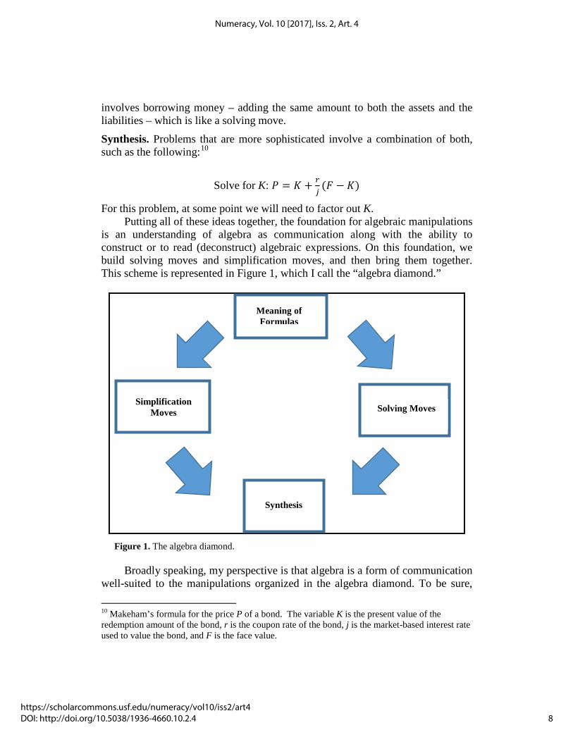
For this problem, at some point we will need to factor out K. Putting all of these ideas together, the foundation for algebraic manipulations

is an understanding of algebra as communication along with the ability to construct or to read (deconstruct) algebraic expressions. On this foundation, we build solving moves and simplification moves, and then bring them together. This scheme is represented in Figure 1, which I call the “algebra diamond.”

Figure 1. The algebra diamond.

Broadly speaking, my perspective is that algebra is a form of communication well-suited to the manipulations organized in the algebra diamond. To be sure,

10 Makeham’s formula for the price P of a bond. The variable K is the present value of the redemption amount of the bond, r is the coupon rate of the bond, j is the market-based interest rate used to value the bond, and F is the face value.

Meaning of Formulas

Simplification Moves Solving Moves

Synthesis

8



there are many topics in algebra textbooks that do not fit this description – such as graphing functions. Strictly speaking, those are topics in other mathematical domains, such as analysis. I do not mean to suggest that we should avoid teaching those topics in a class called “algebra,” but I think it is helpful to acknowledge, at least to ourselves, that the term “algebra” may be more limited than textbook and course content may suggest..

Difficulty Levels

My perspective on algebra has led me to hypothesize four difficulty levels for solving formulas for a specified variable. The hypothesized levels are as follows:

1. Beginner: Can solve multistep equations for variables by applying inverse operations in reverse order (“reverse and invert”).

A beginner could solve the following:

Solve for Q: 𝐿 = �𝑄𝐺− 12�

2

2. Intermediate: Can solve problems requiring a combination of reverse and invert with “prefabricated moves.”

An intermediate student could solve the following:

Solve for T: 𝑌 = �𝑅𝑇�2

Note that to apply the “reverse and invert” strategy to a problem such as this one requires us to think of taking reciprocals as an operation. This concept is not unreasonable in and of itself, but it may be confusing for students.

3. Advanced: Can solve problems requiring a combination of reverse and invert with prefabricated moves in which we may have to treat expressions as objects to be manipulated. An advanced student can solve the following:

Solve for W: 𝐸 = 12 − 𝑃𝑊

This problem can be solved with two “swaps.” First, swap E for 𝑃𝑊

to

obtain 𝑃𝑊

= 12 − 𝐸. Then swap W for 12–E. The second swap is not just one variable for another, but rather one variable for an expression (12–E). Treating that expression as an object to which we can apply inverse operations is what differentiates the third level from the second level.

4. Mastery: Can solve problems requiring a combination of reverse and invert, prefabricated moves, and simplification moves in which sometimes

9



we have to treat expressions as objects to be manipulated. A master could solve the following problem:

Solve for K: 𝐽 = 𝐿 − (𝐾 + 𝐾𝐹) So how does algebraic manipulation fit with quantitative reasoning? We turn

to this question next.

Quantitative Reasoning and Algebra: Does the Shoe Fit? To me, one hallmark of quantitative reasoning is the solving of contextualized problems using mathematical concepts. As such, an approach to algebraic manipulations, if couched within authentic and realistic contexts, can certainly fit well with quantitative reasoning. Moreover, an approach to algebra as communication that treats algebraic manipulations within the framework of the algebra diamond encourages purposefully knowing what you are doing and why you are doing it, another aspect of quantitative reasoning.

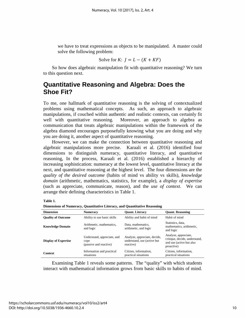
However, we can make the connection between quantitative reasoning and algebraic manipulations more precise. Karaali et al. (2016) identified four dimensions to distinguish numeracy, quantitative literacy, and quantitative reasoning, In the process, Karaali et al. (2016) established a hierarchy of increasing sophistication: numeracy at the lowest level, quantitative literacy at the next, and quantitative reasoning at the highest level. The four dimensions are the quality of the desired outcome (habits of mind vs ability vs skills), knowledge domain (arithmetic, mathematics, statistics, for example), a display of expertise (such as appreciate, communicate, reason), and the use of context. We can arrange their defining characteristics in Table 1.

Table 1. Dimensions of Numeracy, Quantitative Literacy, and Quantitative Reasoning Dimension Numeracy Quant. Literacy Quant. Reasoning

Quality of Outcome Ability to use basic skills Ability and habit of mind Habit of mind

Knowledge Domain Arithmetic, mathematics, and logic

Data, mathematics, arithmetic, and logic

Statistics, data, mathematics, arithmetic, and logic

Display of Expertise Understand, appreciate, and cope (passive and reactive)

Analyze, appreciate, decide, understand, use (active but reactive)

Analyze, appreciate, critique, decide, understand, and use (active but also proactive)

Context Information and practical situations

Citizen, information, practical situations

Citizen, information, practical situations

Examining Table 1 reveals some patterns. The “quality” with which students interact with mathematical information grows from basic skills to habits of mind.

10



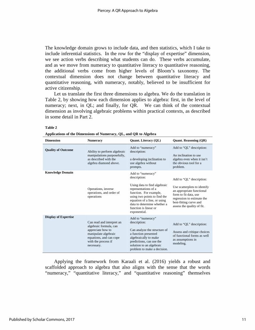
The knowledge domain grows to include data, and then statistics, which I take to include inferential statistics. In the row for the “display of expertise” dimension, we see action verbs describing what students can do. These verbs accumulate, and as we move from numeracy to quantitative literacy to quantitative reasoning, the additional verbs come from higher levels of Bloom’s taxonomy. The contextual dimension does not change between quantitative literacy and quantitative reasoning, with numeracy, notably, believed to be insufficient for active citizenship.

Let us translate the first three dimensions to algebra. We do the translation in Table 2, by showing how each dimension applies to algebra: first, in the level of numeracy; next, in QL; and finally, for QR. We can think of the contextual dimension as involving algebraic problems within practical contexts, as described in some detail in Part 2.

Table 2

Applications of the Dimensions of Numeracy, QL, and QR to Algebra

Dimension Numeracy Quant. Literacy (QL) Quant. Reasoning (QR)

Quality of Outcome Ability to perform algebraic

manipulations purposefully, as described with the algebra diamond above.

Add to “numeracy” description: a developing inclination to use algebra without prompts.

Add to “QL” description: An inclination to use algebra even when it isn’t the obvious tool for a problem.

Knowledge Domain

Operations, inverse operations, and order of operations

Add to “numeracy” description: Using data to find algebraic representations of a function. For example, using two points to find the equation of a line, or using data to determine whether a function is linear or exponential.

Add to “QL” description: Use scatterplots to identify an appropriate functional form to fit data, use regression to estimate the best-fitting curve and assess the quality of fit.

Display of Expertise Can read and interpret an algebraic formula, can appreciate how to manipulate algebraic equations, and can cope with the process if necessary.

Add to “numeracy” description: Can analyze the structure of a function presented algebraically to make predictions, can use the solution to an algebraic problem to make a decision.

Add to “QL” description: Assess and critique choices of functional forms as well as assumptions in modeling.

Applying the framework from Karaali et al. (2016) yields a robust and

scaffolded approach to algebra that also aligns with the sense that the words “numeracy,” “quantitative literacy,” and “quantitative reasoning” themselves

11



suggest. Note that the algebraic manipulations I describe in the context of the algebra diamond align best with “numeracy.”

Part 2: Implementation The value of the theory in Part 1 manifests in how it is implemented in the classroom. In this second part of the paper, we describe the course materials, both in general and in detail, that were inspired by the theory and background. These course materials illustrate what a quantitative approach to algebra looks like in practice. The materials are followed by data that show how the skills of students who have been exposed to this approach compare to those who have taken courses in the traditional algebra and calculus sequence.

Course Materials The course materials comprise a six-week module, which is split into two units. The algebra diamond and other concepts in Part 1 form the “back-end” – embedded in the design but not necessarily shared with students. The materials were written for college business students who place into a developmental algebra-1 course. Almost every lesson involves at least one problem or exercise grounded in contextual meaning. However, the reader will note that as the module progresses, many of the exercises are not couched in a scenario. Rather, most exercises involve manipulating business formulas that themselves have meaning (with variables defined in the supplement) that is not itself addressed within the specific problem. There are a few formulas that were cooked up but have no apparent meaning. In the discussion below, variables are defined (mostly in footnotes) for every formula that has meaning,

Overview of the Course

The course that these materials come from is called Quantitative Reasoning for Professionals (QRP). It is a two-semester sequence where each semester carries 4 credits. Students who place into developmental algebra-1 start with the first-semester course, and those who place into intermediate algebra take only the second course. Each section has between 20 and 25 students. I designed QRP and wrote the materials. The sequence is delivered at Ferris State University, a medium-sized, public institution in a rural area of central Michigan. So far, besides myself, two tenure-track faculty and one adjunct faculty have taught the sequence. I revise and distribute the course materials as a course pack every year. The description below represents the third edition; the fourth is being prepared.

The best description of the content of QRP is as a hybrid quantitative reasoning and algebra course. Business students will be taking accounting and

12



finance courses that require stronger algebraic reasoning than a typical quantitative reasoning course would offer. On the other hand, at Ferris State, business students do not take a business calculus course and do not need much of what is included in typical algebra courses. Rather, they need to be able to reason with data and quantitative objects. Consequently, a quantitative reasoning approach that includes algebra is called for, and the courses were designed as an answer to that call. The course content is organized into units as indicated in Table 3.

Table 3. The Mathematical Content in Quantitative Reasoning for Professionals (QRP). First Semester Units Second Semester Units

1. Proportional Reasoning 1. Linear Functions 2. Data-Based Decisions 2. Exponential Functions 3. Constructing and Deconstructing Algebraic

Representations 3. Logarithms

4. Manipulating Algebraic Formulas 4. Linear and Nonlinear Analysis

The materials described in this paper are used in the third and fourth unit of the first semester. As implied by Part 1, if we are being careful about our terms, the students who are successful in Units 3 and 4 would be described best as “numerate” in algebra. In the second semester, the level at which students are expected to use algebra mostly fits the “quantitative literacy” characteristics described in Part 1, but by the end we also reach the “quantitative reasoning” level. For example, at the end of the course, students use scatterplots with various combinations of linear and logarithmic scales to select an appropriate model for selected data sets, run appropriate regressions to estimate those models, use those models to make predictions, and assess the strength of their assumptions. We share some sample problems from the second course below.

The Role of Excel

The course materials use Excel heavily, both to motivate the use of algebra and to help students understand the computational directions in a given algebraic formula. Spreadsheets are known to enhance quantitative reasoning and have been implemented in a variety of courses as noted in numerous papers in this journal (e.g., Steele and Kiliç-Bahi 2008, Gaze 2010, 2014, Vacher and Lardner 2010, Frith 2012, Lehto and Vacher 2012, Mayfield and Dunham 2015, Ricchezza and Vacher 2017).

Algebra instruction has been enhanced with Excel by others, with varying degrees of success. Friedlander (1998) used Excel in a beginning algebra course at an Israeli middle school and found that the ability to “click” on a cell reference for a variable formed a cognitive link between arithmetic and formal algebra. Stephens (2003) found that students were unlikely to take advantage of extra-

13



credit assignments using Excel, but those who did so enjoyed the assignments. Neurath and Stephens (2006) found that although using Excel in a high school algebra course led to only a slight improvement in student achievement, it helped narrow the gap between the high and low achievers and led to improved student attitudes. Lehto and Vacher (2012) found that the need to learn to use Excel was not a barrier to learning course content, but also that implementation success depends on the instructor’s pedagogical perspective.

In this course, we begin using Excel at the beginning of the second unit.11 By the time the students encounter the algebra units, they have developed comfort and facility with the basic functionality of Excel. At the beginning of Unit 3, we introduce algebraic formulas as tools to “process” data – transforming raw, observable data into a measurement that is useful for evaluation or decision making. The raw data are found in an Excel spreadsheet. Students have to construct the formula they need, and then “program” Excel to use that formula. The ability to “copy and paste” or simply “drag” the formula to the rest of the column reinforces the idea that algebra simply codifies an arithmetic computation. As the course progresses, students have a formula but have to solve it for a different variable to find the missing data in their Excel spreadsheets. The “copy and paste” or “drag” functionality reinforces the idea that when we solve a formula for another variable, we are solving infinitely many one-variable equations simultaneously.

As mentioned in Part 1, algebra is a natural mode of communication when working with Excel. Anecdotally, I have noticed that students like to start with the data in the spreadsheet before working with pencil-and-paper. This observation suggests to me that they find the spreadsheets motivating. I have noticed that as students begin to work through this module, several students report out their formulas using cell references as their variables. This tendency appears to illustrate the role Friedlander (1998) assigned to Excel in students’ developing conception of algebra. With guidance, this approach evolves to using standard mathematical variables. This evolution promotes a discussion of what a choice of variable communicates to your audience, whether Excel or a human audience.

Inquiry-Based Learning

The course materials are designed for inquiry-based learning (IBL). Yoshinobu and Jones (2012) define IBL as an “instructional paradigm” in which

Students actively participate in contributing their mathematical ideas to solve problems, rather than applying teacher-demonstrated techniques to similar exercises. The instructor facilitates student progress, ensuring that the class can move toward increasingly sophisticated ways of thinking.

11 In the fourth edition (of my course materials), in its early stages as of this writing, we are starting much earlier with Excel, introducing it at the fifth class meeting.

14



The materials in the course consist of “explorations” – guided, inquiry-based lessons. Part of the goal of the course is for students to solve novel problems, and IBL is a tool that has shown some success in this regard (Housman and Porter 2003, Kwon, Rasmussen and Allen 2005, Smith 2005, Chappell 2006, Rasmussen and Kwon 2007, Selden and Selden 2013, Kohan and Laursen 2014, Ellis, et al. 2015). In particular, well-designed IBL courses can help students learn to solve problems independently without being given a “template” or a procedure for every problem type, thereby improving problem-solving skills and reversing unhealthy beliefs about mathematics (Schoenfeld 1988, Yohsinobu and Jones 2012). When students learn in this way, they begin to tap into their reasoning skills and rely less on incomplete or incorrectly remembered procedures (Stigler et al. 2010).

The classic version of IBL is the Moore Method, named for R.L. Moore12 who was a mathematician at the University of Texas-Austin from 1920 to 1969. The Moore Method, applied to upper division or graduate mathematics courses, involves providing students with definitions only, and the students fill in the examples and all of the proofs themselves, giving presentations to the class and subjecting their work to the criticism of their classmates. Moore himself did not allow students to speak with one another nor consult any materials as they did their work, but most practitioners today relax these rules, applying the “Modified Moore Method” (e.g., Jones 1977, Chalice 1995, and Mahavier 1999).

Applying the Moore method to a freshman course for students who place into developmental algebra may be a bit daunting. Rather, our approach to IBL for this population involves more “guided inquiry” – that the explorations involve carefully sequenced questions designed to start from prior student knowledge and lead students to some new concept, and then ask students to apply that concept to a new problem.13 In addition, the explorations are contextualized. Most are rooted in authentic, business applications. Applications are used not only to motivate students, but also to situate learning in an environment where we expect meaning to be constructed and concepts to be transferrable to other courses. To be sure, in the spirit of inquiry, some explorations are open-ended. For example, the first exploration in Unit 3 (described below) asks students to come up with a mathematical process to measure “fry efficiency.” The stakes in these 12 I acknowledge that Moore’s intellectual heritage comes loaded with his history of exclusionary practices, including refusals to allow African American students to take his classes. Recognizing Moore’s contributions to teaching and learning mathematics should in no way be considered an endorsement of his exclusionary practices. 13 This design approach resembles, but does not precisely emulate, the cycle of learning that is part of the theory underlying Process-Oriented Guided Inquiry Learning (POGIL) (e.g., Bénéteau et. al. 2017). Current revisions for a fourth edition of the course materials are bringing the design closer in line with POGIL.

15



explorations are low, and students are encouraged to try different approaches, reflect on those approaches, take risks, and pose questions.

Typically, we start class by briefly introducing any mathematical definitions and the business context, after which students work through the explorations in small groups. The instructor circulates around the room, checking on student progress and responding to questions. Every five to ten minutes, the class pauses to discuss what they have done and present their work, before returning to small-group work. Sometimes the presentations are formal, with students walking through their work at the board. Other times we just share our ideas from our seats. While we have not measured the impact on “soft skills” such as communication and collaboration, we have anecdotally observed growth. For more detail concerning the use of inquiry-based learning in this course, see Piercey and Militzer (in press).

A deeper understanding of algebra and development of the framework described above is compatible with IBL. Especially because we are teaching students who have been introduced to algebra before, developing a framework using constructivist approaches helps activate prior knowledge, correct misconceptions, and put that prior knowledge into a useful organization that students can access to solve problems.

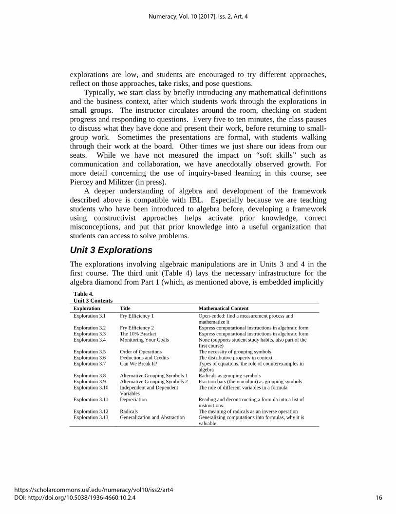
Unit 3 Explorations

The explorations involving algebraic manipulations are in Units 3 and 4 in the first course. The third unit (Table 4) lays the necessary infrastructure for the algebra diamond from Part 1 (which, as mentioned above, is embedded implicitly

Table 4. Unit 3 Contents Exploration Title Mathematical Content Exploration 3.1 Fry Efficiency 1 Open-ended: find a measurement process and

mathematize it Exploration 3.2 Fry Efficiency 2 Express computational instructions in algebraic form Exploration 3.3 The 10% Bracket Express computational instructions in algebraic form Exploration 3.4 Monitoring Your Goals None (supports student study habits, also part of the

first course) Exploration 3.5 Order of Operations The necessity of grouping symbols Exploration 3.6 Deductions and Credits The distributive property in context Exploration 3.7 Can We Break It? Types of equations, the role of counterexamples in

algebra Exploration 3.8 Alternative Grouping Symbols 1 Radicals as grouping symbols Exploration 3.9 Alternative Grouping Symbols 2 Fraction bars (the vinculum) as grouping symbols Exploration 3.10 Independent and Dependent

Variables The role of different variables in a formula

Exploration 3.11 Depreciation Reading and deconstructing a formula into a list of instructions.

Exploration 3.12 Radicals The meaning of radicals as an inverse operation Exploration 3.13 Generalization and Abstraction Generalizing computations into formulas, why it is

valuable

16



in the design). This unit is designed to guide students to look at algebraic representations as lists of instructions with variables. As mentioned above, the idea is to motivate algebraic formulas as tools to “process” data. The fourth unit (Table 5) leads students around the rest of the algebra diamond.

Explorations 3.1 and 3.2 deal with “fry efficiency” at a fast food franchise. The students are given an Excel spreadsheet with data that a manager would collect on a nightly basis. The data include measurements such as the number of fry products sold (read off a receipt) and inventory counts. The students’ job is to figure out how to use these data to measure how efficiently that franchise is using their fries, and this “process” (it is just a formula) has to be programmed into Excel. In effect, students are “algebrafying” the way they use data, and Excel forces them into using symbolic representations. The difference between 3.1 and 3.2 is how much information is given. For 3.1, students are given nothing but the Excel sheet. This problem is open ended, and we do not necessarily expect students to complete it; rather, we want students to have some experience tackling something unscripted and reflect on the process. Some students completely solve the problem by the end of 3.1, while others are able to make progress on one small piece of it. In 3.2, we give them a “form” that is used by managers to compute fry efficiency each evening, and students translate that form into an algebraic formula. Students respond well to this exploration due to its realism. Indeed, I got the idea from my own experience as a fast food manager.

The fry efficiency explorations are followed by an exploration in which students reduce the 1040 EZ tax form into a formula that they can program into Excel. We limit ourselves to the lowest tax bracket in force (at present, the 10% bracket). The purpose of this exploration is to take what students learned with fry efficiency and apply it in a different context, allowing it to sink deeper. This example is dealt with further in the next two explorations (skipping for the purpose of discussion Exploration 3.4, which is the last in a series of study-habits explorations embedded in the course14). Exploration 3.5 reviews order of operations and applies it to the operations involved in calculating taxes. At first, students find it counterintuitive that the steps that we need to apply in order to calculate our taxes do not follow order of operations. This cognitive dissonance raises the need for grouping symbols and explains their importance. In Exploration 3.6, the distributive property is used to investigate the difference 14 Including study skills explorations was inspired by the design of the Dana Center New Mathways Project (NMP). In NMP, the foundational mathematics course is linked with a study skills course. See http://www.utdanacenter.org/higher-education/new-mathways-project/ (accessed by author on Jan. 20, 2017). We did not have the luxury of doing so with QRP, so we embedded a handful of study skills explorations into the course which culminate in a project requiring students to use data to assess progress toward a self-identified goal. Based on our anecdotal observations, we are not convinced that our approach to implementing this idea has been successful to date.

17



http://www.utdanacenter.org/higher-education/new-mathways-project/

between a deduction (which is applied before the tax rate) and a credit (which is applied after the tax rate).

In Exploration 3.7, we introduce the difference between conditional equations and identities. The main purpose of this exploration and those that follow are to help reduce student errors such as “distributing exponents” (for example, asserting that (𝑎 + 𝑏)2 = 𝑎2 + 𝑏2). In order to go beyond the few examples that there is time to address, we focus on helping students to look for counterexamples when they sense doubt about a particular move. This habit of mind is based on an important point about mathematical argumentation: examples can be used to prove that an equation is not an identity, but not to prove that an equation is an identity.

Explorations 3.8 – 3.9 use counterexamples and the distinction between conditional equations and identities to probe the order of operations further. In particular, we look closely at alternative grouping symbols, such as radicals, fraction bars, and absolute value bars. Following numerical calculations with questions about algebra help students learn how these symbols fit into the order of operations. These explorations are frequently turning points for students – the relationship between algebra and arithmetic becomes clearer.

Explorations 3.10 – 3.11 are about reading formulas and bring this unit full circle. First, we address identifying the dependent variable from context. Students are given the future value formula:

𝐹𝐹 = 𝑃𝐹(1 + 𝑟)𝑛 Students describe scenarios in which each of the given variables is the dependent variable. This exercise becomes useful later when we want to manipulate formulas. In 3.11, students are given formulas and asked to reduce them to a list of instructions. This activity is the reverse of what we started the unit with – turning instructions into formulas. At the end of 3.11, students are asked to make a form for computing the declining balance depreciation expense:15

𝐷𝐵𝐷𝐸 = �𝐶𝐶𝐶 ∙ 𝑃𝑃𝐸𝐸𝐿

� �1 −𝑃𝑃𝐸𝐸𝐿

�𝑛−1

This exploration turns the fry efficiency exploration on its head. Exploration 3.12 was created because students had trouble connecting the

notation for radicals to their role as inverse operations for exponents (in the limited case when we want to find an unknown base). Students are encouraged to create their own notation first, and then compare to the established notation. 15 In this formula, DBDE is the periodic expense for depreciation when using the declining balance depreciation technique (in which the value of the asset depreciates exponentially), CST is the initial cost of the asset, EUL is the estimated useful life in years, PM is a preselected percentage multiplier, and n is the age of the asset in years.

18



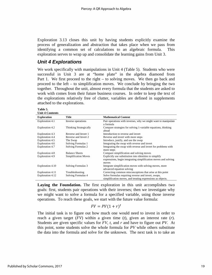
Exploration 3.13 closes this unit by having students explicitly examine the process of generalization and abstraction that takes place when we pass from identifying a common set of calculations to an algebraic formula. This exploration serves to wrap up and consolidate the learning gains from Unit 3.

Unit 4 Explorations

We work specifically with manipulations in Unit 4 (Table 5). Students who were successful in Unit 3 are at “home plate” in the algebra diamond from Part 1. We first proceed to the right – to solving moves. We then go back and proceed to the left – to simplification moves. We conclude by bringing the two together. Throughout the unit, almost every formula that the students are asked to work with comes from their future business courses. In order to keep the text of the explorations relatively free of clutter, variables are defined in supplements attached to the explorations. Table 5. Unit 4 Contents Exploration Title Mathematical Content Exploration 4.1 Inverse operations Pair operations with inverses, why we might want to manipulate

a formula Exploration 4.2 Thinking Strategically Compare strategies for solving 1-variable equations, thinking

ahead Exploration 4.3 Reverse and Invert 1 Introduction to reverse and invert Exploration 4.4 Reverse and Invert 2 Reverse and invert with more steps Exploration 4.5 The Swap Introduce, justify, and use the swap Exploration 4.6 Solving Formulas 1 Integrating the swap with reverse and invert Exploration 4.7 Solving Formulas 2 Integrating the swap with reverse and invert for problems with

more steps Exploration 4.8 Balance Sheets Compare simplification and solving moves Exploration 4.9 Simplification Moves Explicitly use substitution into identities to simplify

expressions, begin integrating simplification moves and solving moves

Exploration 4.10 Solving Formulas 3 Integrate simplification moves with solving moves, more advanced equation solving

Exploration 4.11 Troubleshooting Correcting common misconceptions that arise at this point Exploration 4.12 Solving Formulas 4 Solve formulas requiring reverse and invert, swaps,

simplification moves, and treating expressions as objects.

Laying the Foundation. The first exploration in this unit accomplishes two goals: first, students pair operations with their inverses; then we investigate why we might want to solve a formula for a specified variable, using those inverse operations. To reach these goals, we start with the future value formula:

𝐹𝐹 = 𝑃𝐹(1 + 𝑟)𝑡 The initial task is to figure out how much one would need to invest in order to reach a given target (FV) within a given time (t), given an interest rate (r). Students are given specific values for FV, t, and r and have to figure out PV. At this point, some students solve the whole formula for PV while others substitute the data into the formula and solve for the unknown. The next task is to take an

19



Excel spreadsheet with 50 clients who have specified financial targets, time frames, and interest rates and solve the same problem for all simultaneously. This question shows how efficient it is to solve the formula for PV and program the result into the spreadsheet. The task aims to sell the students on the concept.

Exploration 4.2 helps students conceive of using multiple approaches to solving the same problem, and thinking about strategy along the way. We focus on one-variable equations. Students start by solving 2𝑥 + 4 = 10 and then comparing to the equation:

2𝑥 +14

= 10

They solve the second equation in two different ways and evaluate their approaches. Then they compare to solving the equation:

2𝑥 + 14

= 10

They are also directed to solve this equation using two different ways and evaluate the approaches. Along the way, we address the role of inverse operations and some of the choices we face. Students are encouraged to approach the problems in the rest of the unit with a similar attitude.

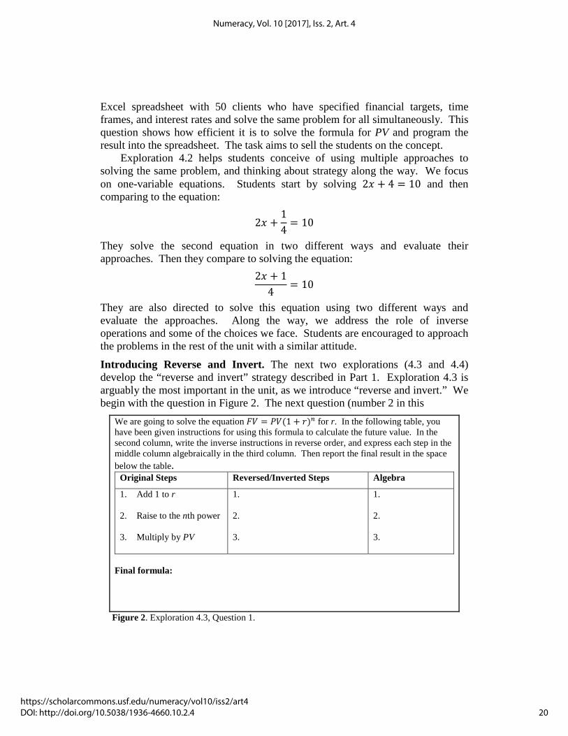
Introducing Reverse and Invert. The next two explorations (4.3 and 4.4) develop the “reverse and invert” strategy described in Part 1. Exploration 4.3 is arguably the most important in the unit, as we introduce “reverse and invert.” We begin with the question in Figure 2. The next question (number 2 in this

We are going to solve the equation 𝐹𝐹 = 𝑃𝐹(1 + 𝑟)𝑛 for r. In the following table, you have been given instructions for using this formula to calculate the future value. In the second column, write the inverse instructions in reverse order, and express each step in the middle column algebraically in the third column. Then report the final result in the space below the table.

Original Steps Reversed/Inverted Steps Algebra

1. Add 1 to r

2. Raise to the nth power

3. Multiply by PV

1. 2. 3.

1. 2. 3.

Final formula:

Figure 2. Exploration 4.3, Question 1.

20



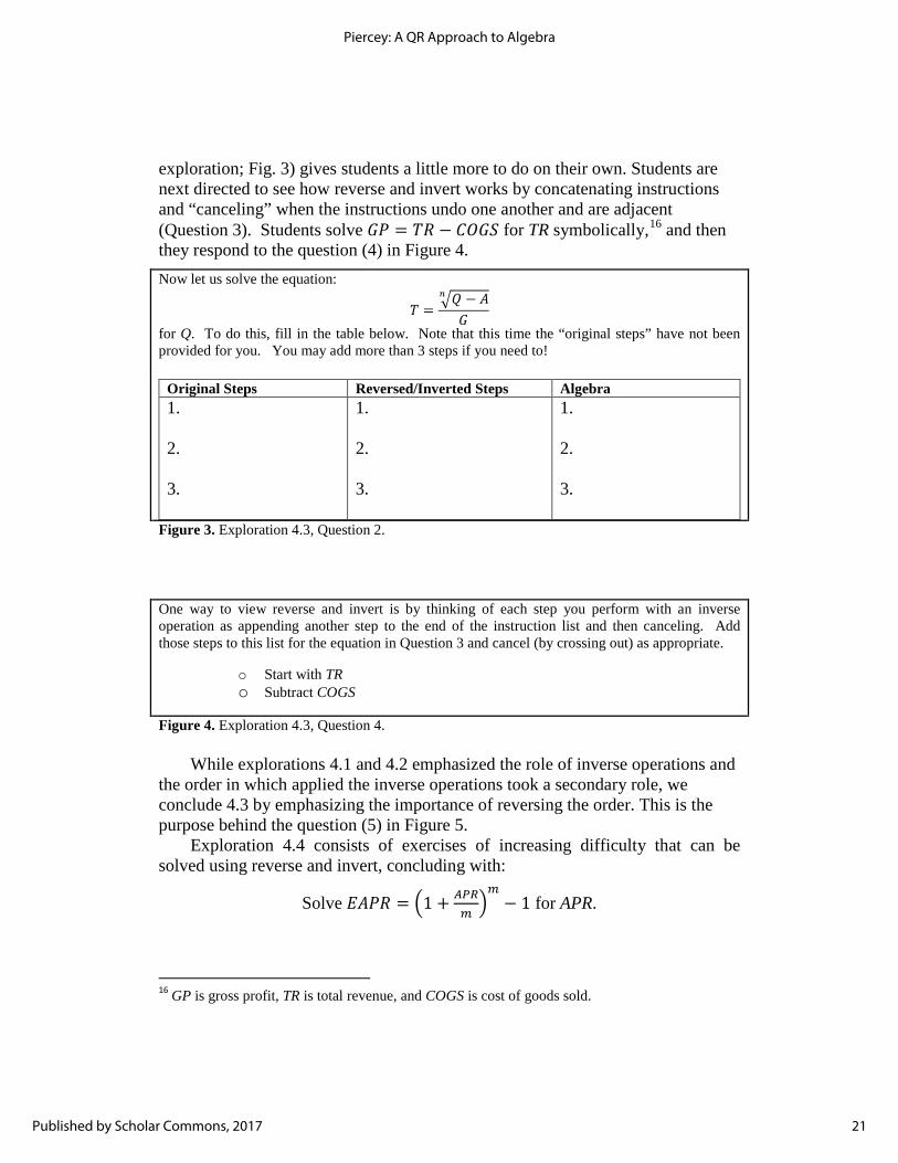
exploration; Fig. 3) gives students a little more to do on their own. Students are next directed to see how reverse and invert works by concatenating instructions and “canceling” when the instructions undo one another and are adjacent (Question 3). Students solve 𝐺𝑃 = 𝐶𝑇 − 𝐶𝐶𝐺𝐶 for TR symbolically,16 and then they respond to the question (4) in Figure 4. Now let us solve the equation:

𝐶 =�𝑄 − 𝐴𝑛

𝐺

for Q. To do this, fill in the table below. Note that this time the “original steps” have not been provided for you. You may add more than 3 steps if you need to!

Original Steps Reversed/Inverted Steps Algebra 1.

2.

3.

1. 2. 3.

1. 2. 3.

Figure 3. Exploration 4.3, Question 2. One way to view reverse and invert is by thinking of each step you perform with an inverse operation as appending another step to the end of the instruction list and then canceling. Add those steps to this list for the equation in Question 3 and cancel (by crossing out) as appropriate.

o Start with TR o Subtract COGS


While explorations 4.1 and 4.2 emphasized the role of inverse operations and the order in which applied the inverse operations took a secondary role, we conclude 4.3 by emphasizing the importance of reversing the order. This is the purpose behind the question (5) in Figure 5.

Exploration 4.4 consists of exercises of increasing difficulty that can be solved using reverse and invert, concluding with:

Solve 𝐸𝐴𝑃𝑇 = �1 + 𝐴𝑃𝑅𝑚�𝑚− 1 for APR.

16 GP is gross profit, TR is total revenue, and COGS is cost of goods sold.

21



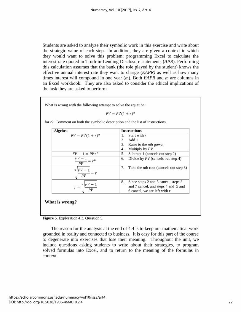
Students are asked to analyze their symbolic work in this exercise and write about the strategic value of each step. In addition, they are given a context in which they would want to solve this problem: programming Excel to calculate the interest rate quoted in Truth-in-Lending Disclosure statements (APR). Performing this calculation assumes that the bank (the role played by the student) knows the effective annual interest rate they want to charge (EAPR) as well as how many times interest will compound in one year (m). Both EAPR and m are columns in an Excel workbook. They are also asked to consider the ethical implications of the task they are asked to perform.

What is wrong with the following attempt to solve the equation:

𝐹𝐹 = 𝑃𝐹(1 + 𝑟)𝑛

for r? Comment on both the symbolic description and the list of instructions.

Algebra Instructions 𝐹𝐹 = 𝑃𝐹(1 + 𝑟)𝑛 1. Start with r

2. Add 1 3. Raise to the nth power 4. Multiply by PV

𝐹𝐹 − 1 = 𝑃𝐹𝑟𝑛 5. Subtract 1 (cancels out step 2) 𝐹𝐹 − 1𝑃𝐹

= 𝑟𝑛 6. Divide by PV (cancels out step 4)

�𝐹𝐹 − 1𝑃𝐹

𝑛= 𝑟

7. Take the nth root (cancels out step 3)

𝑟 = �𝐹𝐹 − 1𝑃𝐹

𝑛

8. Since steps 2 and 5 cancel, steps 3 and 7 cancel, and steps 4 and 5 and 6 cancel, we are left with r

What is wrong?


The reason for the analysis at the end of 4.4 is to keep our mathematical work grounded in reality and connected to business. It is easy for this part of the course to degenerate into exercises that lose their meaning. Throughout the unit, we include questions asking students to write about their strategies, to program solved formulas into Excel, and to return to the meaning of the formulas in context.

22



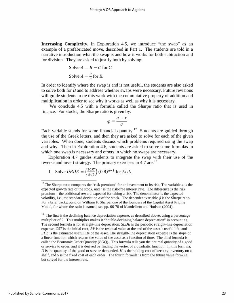
Increasing Complexity. In Exploration 4.5, we introduce “the swap” as an example of a prefabricated move, described in Part 1. The students are told in a narrative introduction what the swap is and how it works for both subtraction and for division. They are asked to justify both by solving:

Solve 𝐴 = 𝐵 − 𝐶 for C

Solve 𝐴 = 𝐵𝐶 for B.

In order to identify where the swap is and is not useful, the students are also asked to solve both for B and to address whether swaps were necessary. Future revisions will guide students to tie this work with the commutative property of addition and multiplication in order to see why it works as well as why it is necessary.

We conclude 4.5 with a formula called the Sharpe ratio that is used in finance. For stocks, the Sharpe ratio is given by:

𝜑 =𝛼 − 𝑟𝜎

Each variable stands for some financial quantity.17 Students are guided through the use of the Greek letters, and then they are asked to solve for each of the given variables. When done, students discuss which problems required using the swap and why. Then in Exploration 4.6, students are asked to solve some formulas in which one swap is necessary and others in which no swaps are necessary.

Exploration 4.7 guides students to integrate the swap with their use of the reverse and invert strategy. The primary exercises in 4.7 are:18

1. Solve 𝐷𝐵𝐷𝐸 = �2𝐶𝐶𝑇𝐸𝐸𝐸

� (0.8)𝑛−1 for EUL.

17 The Sharpe ratio compares the “risk premium” for an investment to its risk. The variable α is the expected growth rate of the stock, and r is the risk-free interest rate. The difference is the risk premium – the additional reward expected for taking a risk. The denominator is the expected volatility, i.e., the standard deviation σ of the stock. The dependent variable ϕ is the Sharpe ratio. For a brief background on William F. Sharpe, one of the founders of the Capital Asset Pricing Model, for whom the ratio is named, see pp. 66-70 of Mandelbrot and Hudson (2004). 18 The first is the declining balance depreciation expense, as described above, using a percentage multiplier of 2. This multiplier makes it “double-declining balance depreciation” in accounting. The second formula is for straight-line deprecation: SLDE is the periodic straight-line depreciation expense, CST is the initial cost, RV is the residual value at the end of the asset’s useful life, and EUL is the estimated useful life of the asset. The straight-line depreciation expense is the slope of a linear function which returns the value of the asset as a function of time. The third formula is called the Economic Order Quantity (EOQ). This formula tells you the optimal quantity of a good or service to order, and it is derived by finding the vertex of a quadratic function. In this formula, D is the quantity of the good or service demanded, H is the holding cost of keeping inventory on a shelf, and S is the fixed cost of each order. The fourth formula is from the future value formula, but solved for the interest rate.

23



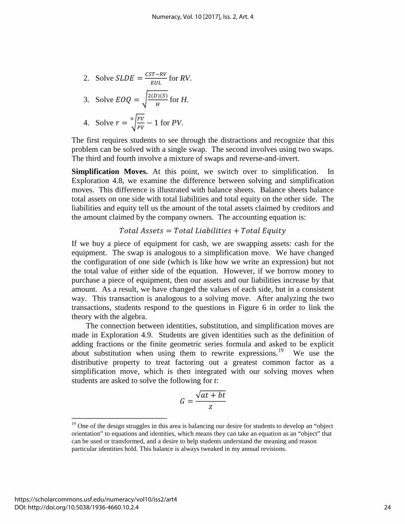
2. Solve 𝐶𝐿𝐷𝐸 = 𝐶𝐶𝑇−𝑅𝑅𝐸𝐸𝐸

for RV.

3. Solve 𝐸𝐶𝑄 = �2(𝐷)(𝐶)𝐻

for H.

4. Solve 𝑟 = �𝐹𝑅𝑃𝑅

𝑛 − 1 for PV.

The first requires students to see through the distractions and recognize that this problem can be solved with a single swap. The second involves using two swaps. The third and fourth involve a mixture of swaps and reverse-and-invert.

Simplification Moves. At this point, we switch over to simplification. In Exploration 4.8, we examine the difference between solving and simplification moves. This difference is illustrated with balance sheets. Balance sheets balance total assets on one side with total liabilities and total equity on the other side. The liabilities and equity tell us the amount of the total assets claimed by creditors and the amount claimed by the company owners. The accounting equation is:

𝐶𝑇𝑇𝑎𝑇 𝐴𝐴𝐴𝐴𝑇𝐴 = 𝐶𝑇𝑇𝑎𝑇 𝐿𝐿𝑎𝑏𝐿𝑇𝐿𝑇𝐿𝐴𝐴 + 𝐶𝑇𝑇𝑎𝑇 𝐸𝐸𝐸𝐿𝑇𝐸 If we buy a piece of equipment for cash, we are swapping assets: cash for the equipment. The swap is analogous to a simplification move. We have changed the configuration of one side (which is like how we write an expression) but not the total value of either side of the equation. However, if we borrow money to purchase a piece of equipment, then our assets and our liabilities increase by that amount. As a result, we have changed the values of each side, but in a consistent way. This transaction is analogous to a solving move. After analyzing the two transactions, students respond to the questions in Figure 6 in order to link the theory with the algebra.

The connection between identities, substitution, and simplification moves are made in Exploration 4.9. Students are given identities such as the definition of adding fractions or the finite geometric series formula and asked to be explicit about substitution when using them to rewrite expressions.19 We use the distributive property to treat factoring out a greatest common factor as a simplification move, which is then integrated with our solving moves when students are asked to solve the following for t:

𝐺 =√𝑎𝑇 + 𝑏𝑇

𝑧

19 One of the design struggles in this area is balancing our desire for students to develop an “object orientation” to equations and identities, which means they can take an equation as an “object” that can be used or transformed, and a desire to help students understand the meaning and reason particular identities hold. This balance is always tweaked in my annual revisions.

24



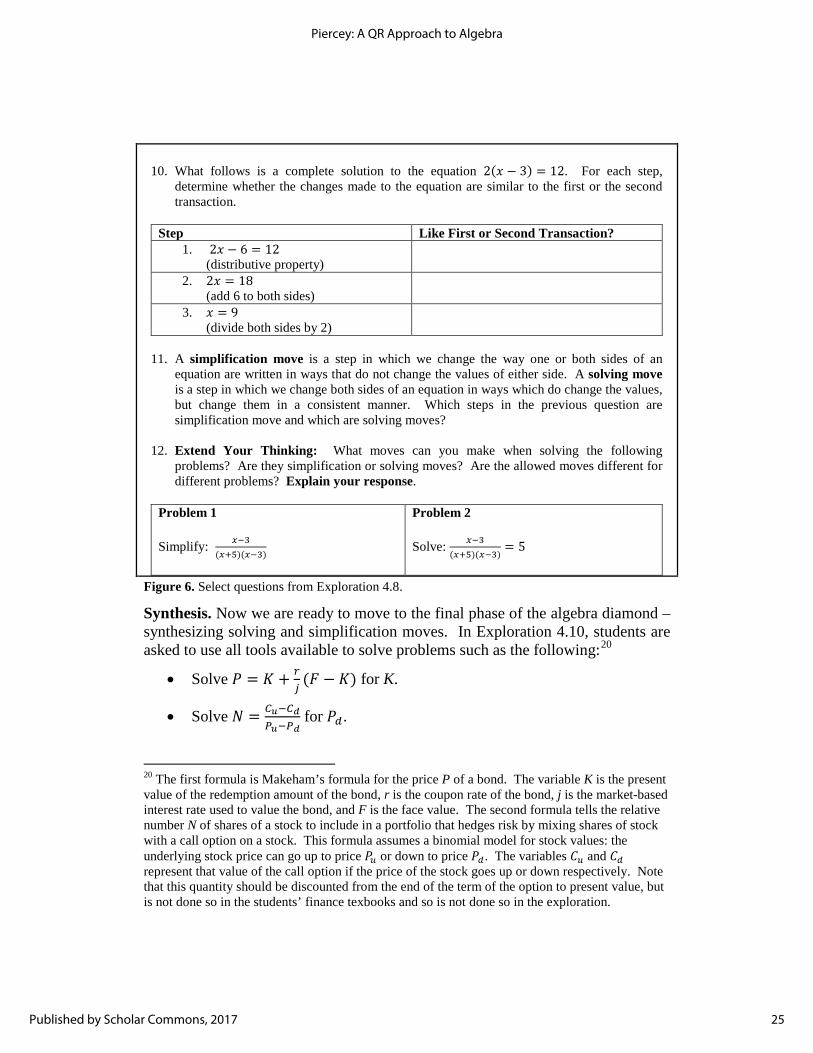
10. What follows is a complete solution to the equation 2(𝑥 − 3) = 12. For each step,

determine whether the changes made to the equation are similar to the first or the second transaction.

Step Like First or Second Transaction?

1. 2𝑥 − 6 = 12 (distributive property)

2. 2𝑥 = 18 (add 6 to both sides)

3. 𝑥 = 9 (divide both sides by 2)

11. A simplification move is a step in which we change the way one or both sides of an

equation are written in ways that do not change the values of either side. A solving move is a step in which we change both sides of an equation in ways which do change the values, but change them in a consistent manner. Which steps in the previous question are simplification move and which are solving moves?

12. Extend Your Thinking: What moves can you make when solving the following

problems? Are they simplification or solving moves? Are the allowed moves different for different problems? Explain your response.

Problem 1 Simplify: 𝑥−3

(𝑥+5)(𝑥−3)

Problem 2 Solve: 𝑥−3

(𝑥+5)(𝑥−3)= 5

Figure 6. Select questions from Exploration 4.8.

Synthesis. Now we are ready to move to the final phase of the algebra diamond – synthesizing solving and simplification moves. In Exploration 4.10, students are asked to use all tools available to solve problems such as the following:20

• Solve 𝑃 = 𝐾 + 𝑟𝑗

(𝐹 − 𝐾) for K.

• Solve 𝑁 = 𝐶𝑢−𝐶𝑑𝑃𝑢−𝑃𝑑

for 𝑃𝑑.

20 The first formula is Makeham’s formula for the price P of a bond. The variable K is the present value of the redemption amount of the bond, r is the coupon rate of the bond, j is the market-based interest rate used to value the bond, and F is the face value. The second formula tells the relative number N of shares of a stock to include in a portfolio that hedges risk by mixing shares of stock with a call option on a stock. This formula assumes a binomial model for stock values: the underlying stock price can go up to price 𝑃𝑢 or down to price 𝑃𝑑. The variables 𝐶𝑢 and 𝐶𝑑 represent that value of the call option if the price of the stock goes up or down respectively. Note that this quantity should be discounted from the end of the term of the option to present value, but is not done so in the students’ finance texbooks and so is not done so in the exploration.

25



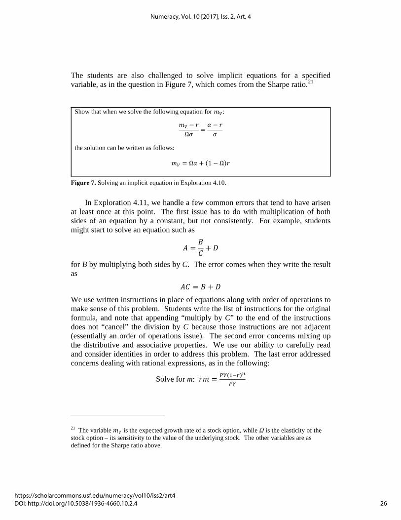
The students are also challenged to solve implicit equations for a specified variable, as in the question in Figure 7, which comes from the Sharpe ratio.21

Show that when we solve the following equation for 𝑚𝑅:

𝑚𝑅 − 𝑟Ω𝜎

=𝛼 − 𝑟𝜎

the solution can be written as follows:

𝑚𝑅 = Ω𝛼 + (1 − Ω)𝑟

Figure 7. Solving an implicit equation in Exploration 4.10.

In Exploration 4.11, we handle a few common errors that tend to have arisen

at least once at this point. The first issue has to do with multiplication of both sides of an equation by a constant, but not consistently. For example, students might start to solve an equation such as

𝐴 =𝐵𝐶

+ 𝐷

for B by multiplying both sides by C. The error comes when they write the result as

𝐴𝐶 = 𝐵 + 𝐷 We use written instructions in place of equations along with order of operations to make sense of this problem. Students write the list of instructions for the original formula, and note that appending “multiply by C” to the end of the instructions does not “cancel” the division by C because those instructions are not adjacent (essentially an order of operations issue). The second error concerns mixing up the distributive and associative properties. We use our ability to carefully read and consider identities in order to address this problem. The last error addressed concerns dealing with rational expressions, as in the following:

Solve for m: 𝑟𝑚 = 𝑃𝑅(1−𝑟)𝑛

𝐹𝑅

21 The variable 𝑚𝑅 is the expected growth rate of a stock option, while Ω is the elasticity of the stock option – its sensitivity to the value of the underlying stock. The other variables are as defined for the Sharpe ratio above.

26



While these issues could have been addressed earlier, we felt it more valuable to let students make these mistakes during their work, and then discuss them in this exploration. That way, those errors are situated in their own work.

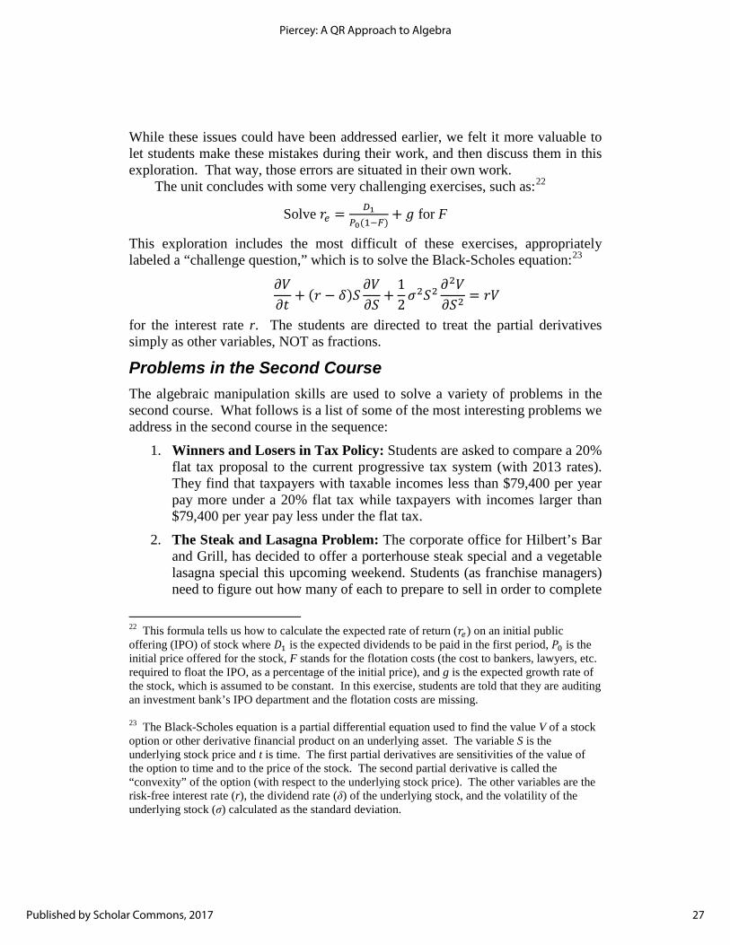
The unit concludes with some very challenging exercises, such as:22

Solve 𝑟𝑒 = 𝐷1𝑃0(1−𝐹)

+ 𝑔 for F

This exploration includes the most difficult of these exercises, appropriately labeled a “challenge question,” which is to solve the Black-Scholes equation:23

𝜕𝐹𝜕𝑇

+ (𝑟 − 𝛿)𝐶𝜕𝐹𝜕𝐶

+12𝜎2𝐶2

𝜕2𝐹𝜕𝐶2

= 𝑟𝐹

for the interest rate r. The students are directed to treat the partial derivatives simply as other variables, NOT as fractions.

Problems in the Second Course

The algebraic manipulation skills are used to solve a variety of problems in the second course. What follows is a list of some of the most interesting problems we address in the second course in the sequence:

1. Winners and Losers in Tax Policy: Students are asked to compare a 20% flat tax proposal to the current progressive tax system (with 2013 rates). They find that taxpayers with taxable incomes less than $79,400 per year pay more under a 20% flat tax while taxpayers with incomes larger than $79,400 per year pay less under the flat tax.

2. The Steak and Lasagna Problem: The corporate office for Hilbert’s Bar and Grill, has decided to offer a porterhouse steak special and a vegetable lasagna special this upcoming weekend. Students (as franchise managers) need to figure out how many of each to prepare to sell in order to complete

22 This formula tells us how to calculate the expected rate of return (𝑟𝑒) on an initial public offering (IPO) of stock where 𝐷1 is the expected dividends to be paid in the first period, 𝑃0 is the initial price offered for the stock, F stands for the flotation costs (the cost to bankers, lawyers, etc. required to float the IPO, as a percentage of the initial price), and g is the expected growth rate of the stock, which is assumed to be constant. In this exercise, students are told that they are auditing an investment bank’s IPO department and the flotation costs are missing. 23 The Black-Scholes equation is a partial differential equation used to find the value V of a stock option or other derivative financial product on an underlying asset. The variable S is the underlying stock price and t is time. The first partial derivatives are sensitivities of the value of the option to time and to the price of the stock. The second partial derivative is called the “convexity” of the option (with respect to the underlying stock price). The other variables are the risk-free interest rate (r), the dividend rate (δ) of the underlying stock, and the volatility of the underlying stock (σ) calculated as the standard deviation.

27



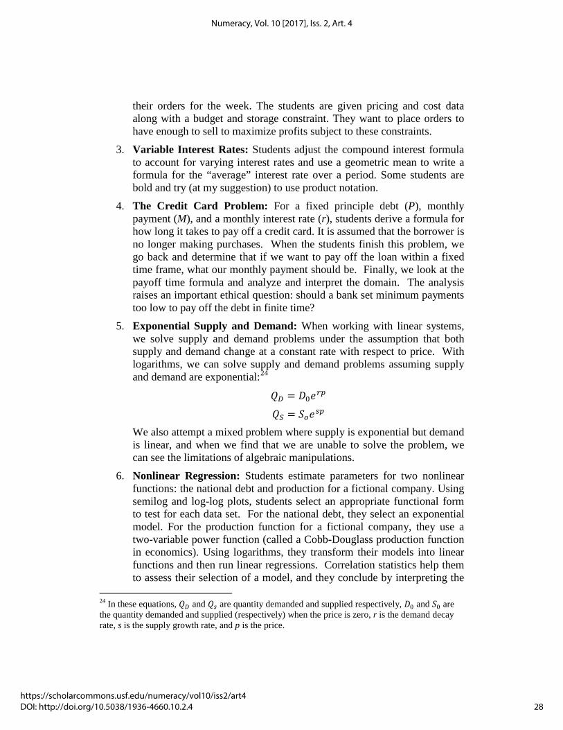
their orders for the week. The students are given pricing and cost data along with a budget and storage constraint. They want to place orders to have enough to sell to maximize profits subject to these constraints.

3. Variable Interest Rates: Students adjust the compound interest formula to account for varying interest rates and use a geometric mean to write a formula for the “average” interest rate over a period. Some students are bold and try (at my suggestion) to use product notation.

4. The Credit Card Problem: For a fixed principle debt (P), monthly payment (M), and a monthly interest rate (r), students derive a formula for how long it takes to pay off a credit card. It is assumed that the borrower is no longer making purchases. When the students finish this problem, we go back and determine that if we want to pay off the loan within a fixed time frame, what our monthly payment should be. Finally, we look at the payoff time formula and analyze and interpret the domain. The analysis raises an important ethical question: should a bank set minimum payments too low to pay off the debt in finite time?

5. Exponential Supply and Demand: When working with linear systems, we solve supply and demand problems under the assumption that both supply and demand change at a constant rate with respect to price. With logarithms, we can solve supply and demand problems assuming supply and demand are exponential:24

𝑄𝐷 = 𝐷0𝐴𝑟𝑟

𝑄𝐶 = 𝐶𝑜𝐴𝑠𝑟 We also attempt a mixed problem where supply is exponential but demand is linear, and when we find that we are unable to solve the problem, we can see the limitations of algebraic manipulations.

6. Nonlinear Regression: Students estimate parameters for two nonlinear functions: the national debt and production for a fictional company. Using semilog and log-log plots, students select an appropriate functional form to test for each data set. For the national debt, they select an exponential model. For the production function for a fictional company, they use a two-variable power function (called a Cobb-Douglass production function in economics). Using logarithms, they transform their models into linear functions and then run linear regressions. Correlation statistics help them to assess their selection of a model, and they conclude by interpreting the

24 In these equations, 𝑄𝐷 and 𝑄𝑠 are quantity demanded and supplied respectively, 𝐷0 and 𝐶0 are the quantity demanded and supplied (respectively) when the price is zero, r is the demand decay rate, s is the supply growth rate, and p is the price.

28



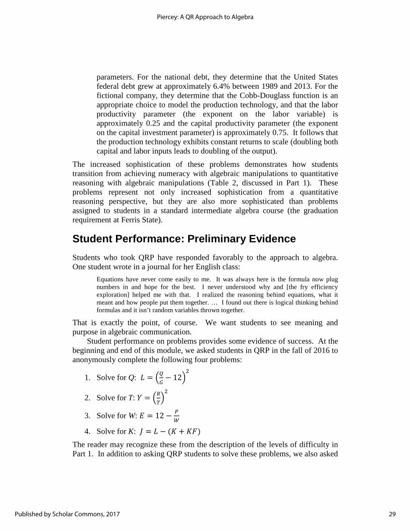
parameters. For the national debt, they determine that the United States federal debt grew at approximately 6.4% between 1989 and 2013. For the fictional company, they determine that the Cobb-Douglass function is an appropriate choice to model the production technology, and that the labor productivity parameter (the exponent on the labor variable) is approximately 0.25 and the capital productivity parameter (the exponent on the capital investment parameter) is approximately 0.75. It follows that the production technology exhibits constant returns to scale (doubling both capital and labor inputs leads to doubling of the output).

The increased sophistication of these problems demonstrates how students transition from achieving numeracy with algebraic manipulations to quantitative reasoning with algebraic manipulations (Table 2, discussed in Part 1). These problems represent not only increased sophistication from a quantitative reasoning perspective, but they are also more sophisticated than problems assigned to students in a standard intermediate algebra course (the graduation requirement at Ferris State).

Student Performance: Preliminary Evidence Students who took QRP have responded favorably to the approach to algebra. One student wrote in a journal for her English class:

Equations have never come easily to me. It was always here is the formula now plug numbers in and hope for the best. I never understood why and [the fry efficiency exploration] helped me with that. I realized the reasoning behind equations, what it meant and how people put them together. … I found out there is logical thinking behind formulas and it isn’t random variables thrown together.

That is exactly the point, of course. We want students to see meaning and purpose in algebraic communication.

Student performance on problems provides some evidence of success. At the beginning and end of this module, we asked students in QRP in the fall of 2016 to anonymously complete the following four problems:

1. Solve for Q: 𝐿 = �𝑄𝐺− 12�

2

2. Solve for T: 𝑌 = �𝑅𝑇�2

3. Solve for W: 𝐸 = 12 − 𝑃𝑊

4. Solve for K: 𝐽 = 𝐿 − (𝐾 + 𝐾𝐹) The reader may recognize these from the description of the levels of difficulty in Part 1. In addition to asking QRP students to solve these problems, we also asked

29



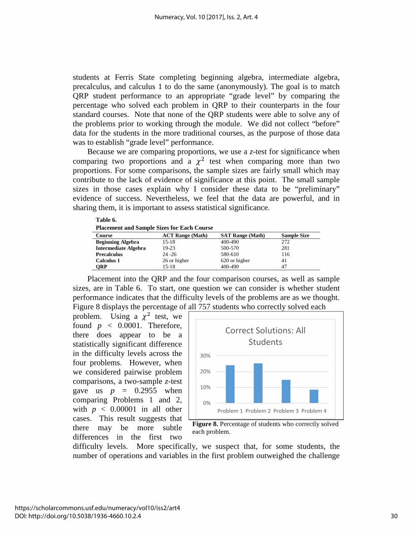
students at Ferris State completing beginning algebra, intermediate algebra, precalculus, and calculus 1 to do the same (anonymously). The goal is to match QRP student performance to an appropriate “grade level” by comparing the percentage who solved each problem in QRP to their counterparts in the four standard courses. Note that none of the QRP students were able to solve any of the problems prior to working through the module. We did not collect “before” data for the students in the more traditional courses, as the purpose of those data was to establish “grade level” performance.

Because we are comparing proportions, we use a z-test for significance when comparing two proportions and a 𝜒2 test when comparing more than two proportions. For some comparisons, the sample sizes are fairly small which may contribute to the lack of evidence of significance at this point. The small sample sizes in those cases explain why I consider these data to be “preliminary” evidence of success. Nevertheless, we feel that the data are powerful, and in sharing them, it is important to assess statistical significance.

Table 6. Placement and Sample Sizes for Each Course Course ACT Range (Math) SAT Range (Math) Sample Size Beginning Algebra 15-18 400-490 272 Intermediate Algebra 19-23 500-570 281 Precalculus 24 -26 580-610 116 Calculus 1 26 or higher 620 or higher 41 QRP 15-18 400-490 47

Placement into the QRP and the four comparison courses, as well as sample sizes, are in Table 6. To start, one question we can consider is whether student performance indicates that the difficulty levels of the problems are as we thought. Figure 8 displays the percentage of all 757 students who correctly solved each problem. Using a 𝜒2 test, we found p < 0.0001. Therefore, there does appear to be a statistically significant difference in the difficulty levels across the four problems. However, when we considered pairwise problem comparisons, a two-sample z-test gave us p = 0.2955 when comparing Problems 1 and 2, with p < 0.00001 in all other cases. This result suggests that there may be more subtle differences in the first two difficulty levels. More specifically, we suspect that, for some students, the number of operations and variables in the first problem outweighed the challenge

Figure 8. Percentage of students who correctly solved each problem.

0%

10%

20%

30%

Problem 1 Problem 2 Problem 3 Problem 4

Correct Solutions: All Students

30



of solving for a denominator in the second, whereas for some other students the opposite was the case.

More importantly, we can use the data to determine how students who took QRP compare to students in the standard four courses (Figs. 9‒12 and Tables 7‒10). The data suggest that the performance by QRP students is around the level of precalculus. The difference between the percentage of QRP students successfully completing each problem and the corresponding percentage of their peers in beginning algebra, as well as from those in the more advanced intermediate algebra course, is practically and statistically significant. The highest percentage of students successfully completing each problem came from calculus (thankfully!). For all but one of the problems, the statistical significance between QRP and calculus is questionable. Given the small sample sizes for calculus and QRP, we cannot form a definitive conclusion.

Figure 9. Percentage of students who correctly solved Problem 1. Table 7. Statistical Tests For Figure 9 Statistical Test p-value z-test, QRP vs. Beginning Algebra p < 0.00001 z-test, QRP vs. Intermediate Algebra p < 0.00001 z-test, QRP vs. Precalculus p = 0.1626 z-test, QRP vs. Calculus 1 p = 0.0805 Chi-squared test, all courses p < 0.00001

0%

10%

20%

30%

40%

50%

60%

70%

BeginningAlgebra

IntermediateAlgebra

Precalculus Calculus 1 QRP

Correct Solutions: Problem 1

31





0%10%20%30%40%50%60%70%80%

BeginningAlgebra

IntermediateAlgebra



0%10%20%30%40%50%60%70%

BeginningAlgebra

IntermediateAlgebra



32




The closest comparison appears to be with precalculus students. The magnitude of the p-values for the first three problems suggests that there may not be a statistically significant difference in these cases, although the small sample size for the QRP students indicates a need for more data. For the fourth problem, QRP students perform better than precalculus students do, and the difference is significant at the .05 level but not the .01 level. This result suggests that a larger sample may yield a statistically significant result.

I should point out that students in QRP were tested before and after a module that was specifically designed to improve algebraic manipulation skills. The instrument itself included two problems that could be solved using “the swap.” Further work should involve developing an instrument that is open to additional prefabricated moves. Finally, note that the QRP students completed this instrument immediately upon concluding the module. A further longitudinal study might yield different results, and could also assess whether students grow from being numerate with algebra to being quantitatively literate and able to quantitatively reason with algebra, as described in Part 1.

Despite these limitations as well as some small sample sizes, the data show promise. I believe part of what we are seeing is the impact of sense-making. Guiding students to identify appropriate steps themselves within the framework of treating algebraic expressions as instructions, appears to lead students to purposefully use solving and simplification moves to unravel the formulas.

0%

10%

20%

30%

40%

50%

60%

BeginningAlgebra

IntermediateAlgebra



33



Another part of what we are seeing comes from contextualization. We create a need for formula manipulation within realistic contexts, aided and abetted by Excel. The relative importance of these factors is unknown at this time – our preliminary success comes from a “cocktail of treatments” so to speak. In future studies, we might conduct interviews and collect qualitative data about the students’ thinking process and their motivation. Nevertheless, our preliminary data suggest that this combination of the “instructions perspective” and contextualization has the potential to lead to improved algebraic reasoning.

Concluding Remarks and Further Questions Numeracy, quantitative literacy, and quantitative reasoning are not “non-algebra.” These terms provide a framework for assessing depth of understanding of knowledge domains from mathematics and statistics. This framework fits well with algebra, at least within my perspective of what we mean by “algebra” and “algebraic manipulations.” This perspective yields a “quantitative reasoning” approach to algebra that can be operationalized and taught. By applying this approach using inquiry-based materials motivated by contextualized problems, students construct an understanding of algebra and develop the skills within the framework of the algebra diamond.

Some preliminary data show the potential this approach has to be effective, notwithstanding limitations. However, using the analysis of Karaali et al. (2016), we note that we are measuring only numeracy with respect to algebra. There are many further questions and directions that can be explored. Can we guide students to use generalized “prefabricated” solving moves besides the swap? What would happen if we treated “negation” and “reciprocation” as operations which invert themselves? Would it be worth the time to guide students to replace inverse operations with inverse elements?

Further down the road, we can ask whether students who complete the second course have achieved my standard for quantitative reasoning with algebra. We can ask if their growth persists into their studies after completing their math courses. We can also look for the impact on affective characteristics, such as math anxiety and beliefs about math. For example, I have some preliminary data that suggest students who complete QRP experience a significantly larger reduction in math anxiety than those who complete a project-based liberal arts math course that eschews algebra and algebraic manipulations (while both sets of students experience a significantly larger reduction than those who take intermediate algebra). My hypothesis is that the students in QRP recognize the algebra we do in class as “math,” while students in the liberal arts math course think something along the lines of “well, that course was nice, but in a real math course…” I won’t know without conducting interviews.

34



There is also a question of whether this course or its materials can be brought to scale. So far at Ferris State, four faculty members have taught the course (including me, the course’s creator). They each taught the course under different circumstances and have found the experience rewarding. The data presented in this paper aggregate the results from three sections of QRP taught by two different instructors, including myself. Additionally, it is appropriate to ask if the course can be adopted for students in other occupational majors, such as health professions. In the near future, I have two plans for scaling and expansion. One plan includes adding nursing and social work students to the audience for the course. This further work involves collaboration with nursing and social work faculty, and it is supported by a grant from the National Science Foundation. The other involves using a faculty learning community to extend the number of instructors teaching the course.

I believe that with QRP, I have stumbled into something with great potential. This paper can serve as an “existence theorem” illustrating that algebra can be addressed within the framework of quantitative reasoning. The students’ performance suggests that quantitative reasoning is a powerful framework for learning algebraic manipulations. The problems students can handle in the second course of the semester serve to underline this promise. There remain a lot of questions to ask, and fertile ground for future research. I invite the readers to join me in this journey.

Acknowledgments I would like to thank all of the instructors who delivered the algebra instrument to their students. I also thank Anil Venkatesh, Erin Militzer, and Harvey Hannah for their willingness to teach QRP. In addition, Kirk Weller has served as a valuable resource and sounding board through course development and assessment studies. I would also like to thank the referees who reviewed this paper for their helpful suggestions. While I wish the final draft was shorter than the initial draft, it seems that whenever I revise papers I am confronting Hyrdra: for every sentence deleted, two more take its place. In addition, I thank Mike May from Saint Louis University, whose Excel-based business calculus course inspired the use of Excel in QRP. Finally, I would like to thank Len Vacher and Eric Gaze, each of whom recommended that I submit this paper to Numeracy.

References Anderson, G., D. Benjamin, and M. Fuss. 1994. “The Determinants of Success in

University Introductory Economics Courses.” Journal of Economic Education 25(Spring): 99–119.

35



Arnon, I., J. Cottrill, E. Dubinsky, A. Oktac, A.R. Fuentes, M. Trigueros, and K. Weller. 2014. APOS Theory: A Framework for Research and Curriculum Development in Mathematics Education. New York: Springer. https://doi.org/10.1007/978-1-4614-7966-6.

Asiala, M., A. Brown, D.J. DeVries, E. Dubinsky, D. Matthews, and J. Thomas. 1996. “A Framework for Research and Development in Undergraduate Mathematics Education. In Kaput et al. 1996, 1–32

Association of American Colleges and Universities (AACU). 2010. Quantitative Literacy VALUE Rubric. Accessed March 29, 2017. http://www.aacu.org/value/rubrics/quantitative-literacy.

Ballard, C.L. and M.F. Johnson. 2004. “Basic Math Skills and Performance in an Introductory Economics Class.” Journal of Economic Education 35(Winter): 3–23. https://doi.org/10.3200/JECE.35.1.3-23.

Bénéteau, C., Z. Guadarrame, J.E. Guerra, L. Lenz, J.E. Lewis, A. Straumanis. 2017. POGIL in the calculus classroom. PRIMUS: Problems, Resources, and Issues in Mathematics Undergraduate Studies. http://doi.org/10.1080/10511970.2016.1233159.

Bennett, J., and B. Briggs. 2014. Using and Understanding Mathematics: A Quantitative Reasoning Approach. 6th ed. Boston: Pearson.

Catalano, M.T. 2010. “College Algebra in Context: A Project Incorporating Social Issues.” Numeracy 3(1): Article 7. http://doi.org/10.5038/1936-4660.3.1.7.

Chappell, K.K. 2006. “Effects of Concept-Based Instruction on Calculus Students’ Acquisition of Conceptual Understanding and Procedural Skill.” In Hitt et al. 2006, 27–60.

Chalice, D. R. 1995. “How to Teach a Class by the Modified Moore Method.” American Mathematical Monthly 102(4): 317–321. https://doi.org/10.2307/2974951.

Dautermann, J. 1992. Using ISETL 3.0: A Language for Learning Mathematics. St. Paul, MN: West Publishing.

Dubinsky, E. 1991. “Reflective Abstraction in Advanced Mathematical Thinking.” In Tall 1991, 95–123.

Ellis, J., K. Hanson, G. Nunez, and C. Rasumussen. 2015. “Beyond Plug and Chug: An Analysis of Calculus 1 Homework.” International Journal of Research in Undergraduate Mathematics Education 1(2): 268–287. https://doi.org/10.1007/s40753-015-0012-z.

Ely, D.P. and L. Hittle. 1990. “The Impact of Math Background on Performance in Managerial Economics and Basic Finance Courses.” Journal of Financial Education. 19(Fall): 59–61.

Friedlander, A. 1998. “An EXCELlent Bridge to Algebra.” The Mathematics Teacher 91(5): 382–383.

36



https://doi.org/10.1007/978-1-4614-7966-6

http://www.aacu.org/value/rubrics/quantitative-literacy

https://doi.org/10.3200/JECE.35.1.3-23

http://doi.org/10.1080/10511970.2016.1233159

http://doi.org/10.5038/1936-4660.3.1.7

http://doi.org/10.5038/1936-4660.3.1.7

https://doi.org/10.2307/2974951

https://doi.org/10.1007/s40753-015-0012-z

Frith, V. 2012. "Quantitative Literacy Interventions at University of Cape Town: Effects of Separation from Academic Disciplines." Numeracy 5(1): Article 3. https://doi.org/10.5038/1936-4660.5.1.3.

Ganter, S.L. and W. Barker, W, eds. 2004. Curriculum Foundations Project: Voices of the Partner Disciplines. Washington, D.C.: Mathematical Association of America.

Ganter, S.L. and W.E. Haver, W.E., eds. 2011. Partner Discipline Recommendations for Introductory College Mathematics and the Implications for College Algebra. Washington, D.C.: Mathematical Association of America.

Gaze, E. 2010. "Creating a Masters in Numeracy Program." Numeracy 3(2): Article 8. https://doi.org/10.5038/1936-4660.3.2.8.———. 2014. “Teaching Quantitative Reasoning: A Better Context for Algebra.” Numeracy 7(1): Article 1. https://doi.org/10.5038/1936-4660.7.1.1.

Geiger, V., H. Forgasz, and M. Goos. 2015. “A Critical Orientation to Numeracy across the Curriculum.” ZDM: Mathematics Education 47(4): 611–624. https://doi.org/10.1007/s11858-014-0648-1.

Green, J.J., C.C. Stone, A. Zegeye, and T.A. Charles. 2007. “Changes in Math Prerequisites and Student Performance in Business Statistics: Do Math Prerequisites Really Matter?” Journal of Economics and Finance Education 6(2): 27–38.

Hamman, K. and D. Kung. 2017. “A Delicate Balance: Quantitative Literacy and Equity.” MAA Focus 36 (6): 14–15.

Harper, E. 1987. “Ghosts of Diophantus.” Educational Studies in Mathematics 18(1): 75⎼90.

Hitt, F., G. Harel, and A. Selden, eds. 2006. Research in Collegiate Mathematics Education, VI. Providence, RI: American Mathematical Society.

Houseman, D. and M. Porter. 2003. “Proof Schemes and Learning Strategies of Above-Average Mathematics Students.” Educational Studies in Mathematics 53(2): 139–158. https://doi.org/10.1023/A:1025541416693.

Jones, F. B. 1977. “The Moore Method.” American Mathematical Monthly 84: 273–277. https://doi.org/10.2307/2318868.

Kaput, J., E. Dubinsky, and A. H. Schoenfeld, eds. 1996. Research in Collegiate Mathematics Education II. Providence, RI: American Mathematical Society.

Karaali, G. 2008. “Word Problems: Reflections on Embedding Quantitative Literacy in a Calculus Course.” Numeracy 1(2): Article 6. http://doi.org/10.5038/1936-4660.1.2.6.

———, E.D. Villafane Hernandez, and J.A. Taylor. 2016. “What’s in a Name? A Critical Review of Definitions of Quantitative Literacy, Numeracy, and Quantitative Reasoning.” Numeracy 9(1): Article 2. http://doi.org/10.5038/1936-4660.9.1.2.

37



https://doi.org/10.5038/1936-4660.5.1.3

https://doi.org/10.5038/1936-4660.3.2.8

https://doi.org/10.5038/1936-4660.7.1.1

https://doi.org/10.1007/s11858-014-0648-1

https://doi.org/10.1023/A:1025541416693

https://doi.org/10.2307/2318868

http://doi.org/10.5038/1936-4660.1.2.6

http://doi.org/10.5038/1936-4660.9.1.2

Kohan, M. and S. Laursen. 2014. “Assessing Long-Term Effects of Inquiry-Based Learning: A Case Study from College Mathematics.” Innovative Higher Education 39: 183–199. https://doi.org/10.1007/s10755-013-9269-9.

Kwon, O., C. Rasmussen, and K. Allen. 2005. “Students’ Retention of Mathematical Knowledge and Skills in Differential Equations.” School Science and Mathematics 105: 227–239. https://doi.org/10.1111/j.1949-8594.2005.tb18163.x.

Lehto, H.L. and H.L. Vacher. 2012. “Spreadsheets across the Curriculum, 4: Evidence of Student Learning and Attitudes about Spreadsheets in a Physical Geology Course.” Numeracy 5(2): Article 5. http://doi.org/10.5038/1936-4660.5.2.5.

Mahavier, W. S. 1999. “What Is the Moore Method?” PRIMUS: Problems, Resources, and Issues in Mathematics Undergraduate Studies 9(4): 339–354. https://doi.org/10.1080/10511979908965940.

Mandelbrot, B. and R.L. Hudson. 2004. The (Mis)Behavior of Markets: A Fractal View of Financial Turbulence. New York: Basic Books.

Mayfield, B., and J. B. Dunham. 2015. "Adapting to a New Core Curriculum at Hood College: From Computation to Quantitative Literacy." Numeracy 8(2): Article 8. https://doi.org/10.5038/1936-4660.8.2.8. Moses, R.P. and C.E. Cobb. 2002. Radical equations: Civil Rights from Mississippi to the Algebra Project. Boston: Beacon Press.

Neurath, R.A. and L. J. Stevens. 2006. “The Effect of Using Microsoft Excel in a High School Algebra Class.” International Journal of Mathematical Education in Science and Technology 37(6): 721–726. https://doi.org/10.1080/00207390600989251.

Piercey, V. and E. Militzer. in press. “An Inquiry-Based Quantitative Reasoning for Business Students.” PRIMUS: Problems, Resources, and Issues in Mathematics Undergraduate Studies, doi:10.1080/10511970.2016.1251519

Raehsler, R.D., K. Hung, C.W. Yang, and T.J. Stuhldreher. 2012. “Are Mathematics, Economics, and Accounting Courses Important Determinants in Financial Management: A rank OrderApproach.” Journal of Economics and Finance Education 11(1): 48–59.

Rasmussen, C. and O.N. Kwon. 2007. “An Inquiry-Oriented Approach to Undergraduate Mathematics.” Journal of Mathematical Behavior 26: 189–194. https://doi.org/10.1016/j.jmathb.2007.10.001.

Ricchezza, V. J., and H. L. Vacher. “A Twenty-Year Look at ‘Computational Geology,’ an Evolving, In-Discipline Course in Quantitative Literacy at the University of South Florida.” Numeracy 10(1): Article 6. https://doi.org/10.5038/1936-4660.10.1.6.

38



https://doi.org/10.1007/s10755-013-9269-9

https://doi.org/10.1111/j.1949-8594.2005.tb18163.x

https://doi.org/10.1111/j.1949-8594.2005.tb18163.x

http://doi.org/10.5038/1936-4660.5.2.5

http://doi.org/10.5038/1936-4660.5.2.5

https://doi.org/10.1080/10511979908965940

https://doi.org/10.5038/1936-4660.8.2.8

https://doi.org/10.1080/00207390600989251

https://doi.org/10.1016/j.jmathb.2007.10.001

https://doi.org/10.5038/1936-4660.10.1.6

Rosenbaum, R. 1986. “Teaching Critical Thinking in the Business Mathematics Course.” Journal of Education for Business. 62(2): 66–69. https://doi.org/10.1080/08832323.1986.10772774.

Schoenfeld, A.J. 1988. “When Good Teaching Leads to Bad Results: The Disasters of ‘Well-Taught’ Mathematics Courses.” Educational Psychologist 23: 145–166. https://doi.org/10.1207/s15326985ep2302_5.

Selden, A. and J. Selden. 2013. “Proof and Problem Solving at the University Level.” The Mathematics Enthusiast 10(1-2): 303–333.

Service, R. 2000. Lenin: A Biography. London: Macmillan Smith, J.C. 2005. “A Sense-Making Approach to Proof: Strategies of Students in

Traditional and Problem-Based Number Theory Courses.” Journal of Mathematical Behavior 25: 73–90. https://doi.org/10.1016/j.jmathb.2005.11.005.

Steele B., and S. Kiliç-Bahi. 2008. "Quantitative Literacy Across the Curriculum: A Case Study." Numeracy 1(2): Article 3. https://doi.org/10.5038/1936-4660.1.2.3. Steen, L.A. 1999. “Numeracy: The New Literacy for a Data-Drenched Society.” Educational Leadership 57(2): 8–13.

———, ed. 2001. Mathematics and Democracy: The Case for Quantitative Literacy. Washington, D.C.: Woodrow Wilson National Fellowship Program.

Stevens, L.J. 2003. “Microsoft Excel as a Supplement to Intermediate Algebra.” International Journal of Mathematical Education in Science and Technology 34(4): 575–579. https://doi.org/10.1080/0020739031000148976.

Stigler, J.W., K.B. Givven, and B.J. Thompson. 2010. “What Community College Developmental Mathematics Students Understand about Mathematics.” MathAMATYC Educator 1(3). 4–16.

Tall, D. ed. Advanced Mathematical Thinking. Dordrecht, the Netherlands: Kluwer Academic Press.

Tunstall, S.L. and M.J. Bossé. 2015. “Promoting Numeracy in an Online College Algebra Course through Projects and Discussions.” Numeracy 8(2): Article 10. http://doi.org/10.5038/1936-4660.8.2.10.

Vacher, H.L. and E. Lardner. 2010. “Spreadsheets Across the Curriculum 1: The Idea and the Resource.” Numeracy 3(2): Article 6. http://doi.org/10.5038/1936-4660.3.2.6.

Wallace, D. 2011. “Parts of the Whole: An Algebra Lesson.” Numeracy 4(2): Article 10. http://doi.org/10.5038/1936-4660.4.2.10.

Yoshinobu, S. and M. Jones. 2012. “The Coverage Issue.” PRIMUS: Problems, Resources, and Issues in Mathematics Undergraduate Studies 22 (4): 303–316. http://doi.org/10.1080/10511970.2010.507622.

Zillmann, D., C. Callison, and R. Gibson. 2009. “Quantitative Media Literacy: Individual Differences in Dealing with Numbers in the News.” Media Psychology 12(4): 394–416. https://doi.org/10.1080/15213260903287275

39



https://doi.org/10.1080/08832323.1986.10772774

https://doi.org/10.1207/s15326985ep2302_5

https://doi.org/10.1016/j.jmathb.2005.11.005

https://doi.org/10.5038/1936-4660.1.2.3

https://doi.org/10.5038/1936-4660.1.2.3

https://doi.org/10.1080/0020739031000148976

http://doi.org/10.5038/1936-4660.8.2.10

http://doi.org/10.5038/1936-4660.3.2.6

http://doi.org/10.5038/1936-4660.4.2.10

http://doi.org/10.1080/10511970.2010.507622

https://doi.org/10.1080/15213260903287275

a quantitative reasoning approach to algebra using inquiry

Documents