A Public dynamic PET brain database for lesion detection andquantification

First Authors: Natalia Martinez, Martin Bertran.Co-authors: Guillermo Carbajal, Alicia Fernandez and Alvaro Gomez.

Abstract— Purpose: Dynamic PET imaging gives insightinto various metabolic processes. Considerable work has beencarried out with the aim of facilitate visual inspection andinterpretation of the studies. However, comparison betweendifferent algorithms and methods is an arduous task. Sourcecodes are rarely distributed, and if available, there is no single,unified public database to test them on. Therefore, turns outmandatory for any new research team, to invest considerabletime and effort in acquiring or creating their own databasebefore diving headlong into research. This paper presents adynamic PET brain database.Methods: The ASIM and STIR software packages are used tosimulate and reconstruct phantoms based on a pharmacokineticmodel activity.Results: There are 18 phantoms in total, each with 5 implantedregions, and with varying lesion activities.Conclusions: Phantoms are made available to the community.We hope this makes intercomparisons between algorithmseasier, as well as accelerate the research process in the area.

I. INTRODUCTION

Functional imaging is a method in medical imaging ofdetecting or measuring changes in metabolism, blood flow,regional chemical composition, and absorption. PositronEmission Tomography (PET) is one amongst these tech-niques, it can produce 3D and 4D (dynamic) images, and itsmost common use is for the exploration of cancer metastasisusing the FDG tracer.

The recent use of dynamic PET scans enables a newrange of analysis techniques, but the lack of a public phan-tom database makes comparing tests between researchers adifficult task, and requires that research groups spend timeand effort making their own database before starting theirresearch work.

This is exemplified in [12], [13], where researchers mustnot only present their work, but create and describe theirprivate database, this consumes valuable research time, aswell as making intercomparisons more tedious.

In this article, we present a public dynamic PET brainphantom database for the FDG tracer. Additionally themethodology used to generate these phantoms using theASIM [3], [8] simulator and the STIR [4] reconstructionsoftware is presented.

II. MATERIALS AND METHODS.

In order to simulate a realistic phantom, it is necessary todefine four main items.

• Anatomy: The volume of interest, as well as the differ-ent regions are defined. In this case, the volume attemptsto emulate the contents of a human head.

Fig. 1: From top to bottom: The labelmap is combined withthe defined activity curves to generate the activity maps.These are used as input for the ASIM simulator, whichoutputs the raw acquisitions (sinograms). These sinogramsare reconstructed using the STIR software to obtain the final4D phantom.

• Activity: Defines how each region’s activity changesover time. To generate this activity, the two compart-ment pharmacokinetical model is used.

• Acquisition: Controls how a given anatomy with a givenactivity is acquired or observed by a dynamic PET scan.To perform the simulated acquisition, we use the ASIMsimulator [3], [8].

• Reconstruction: This process turns the acquired data(sinograms) into an easy to interpret 3D (or 4D) image.Reconstruction is performed using the STIR library [4].

In Figure 1, the workflow used to generate a dynamic PETphantom is outlined.

We now give additional details on the implementation ofeach of the aforementioned steps.

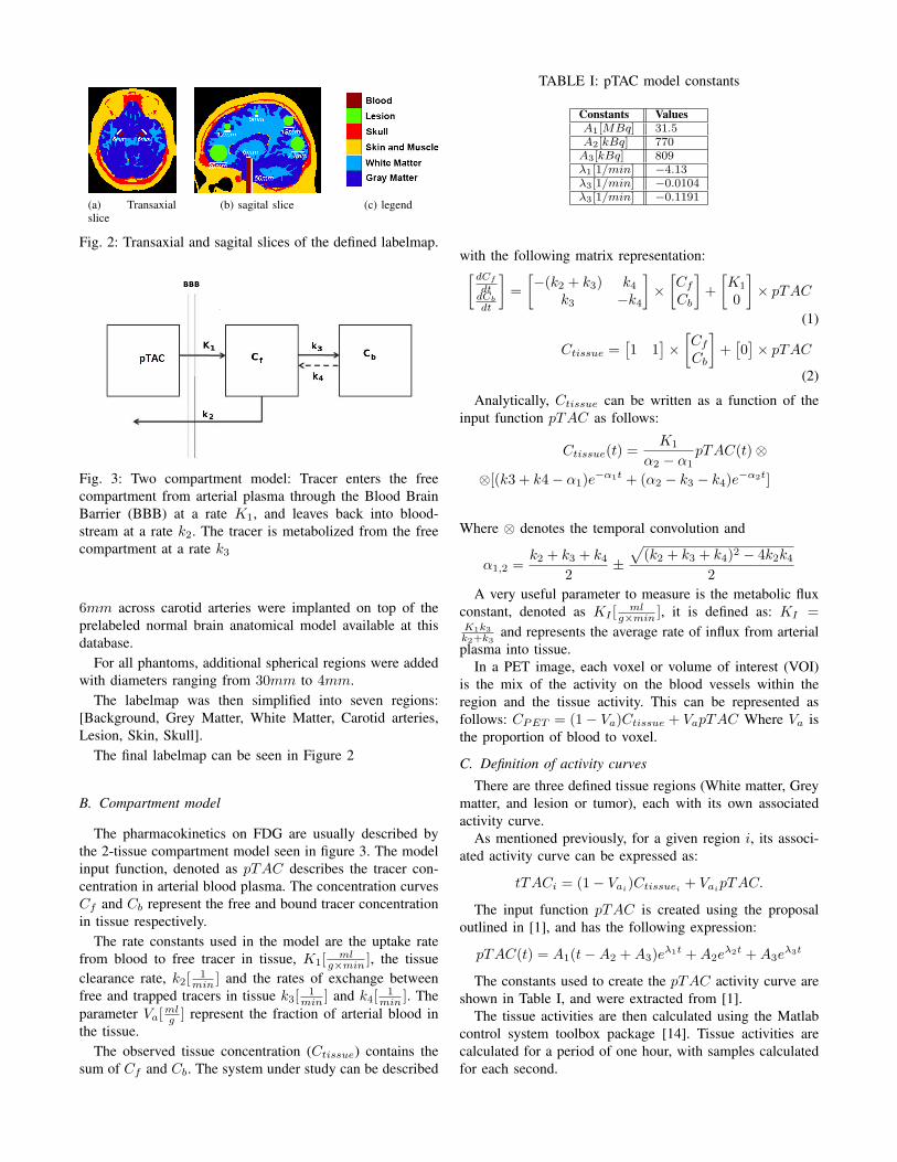
A. Anatomy: Labelmaps

A three-dimensional (3D) software phantom was createdbased on the BrainWeb database [2]. Two 6cm long and

(a) Transaxialslice

(b) sagital slice (c) legend

Fig. 2: Transaxial and sagital slices of the defined labelmap.

Fig. 3: Two compartment model: Tracer enters the freecompartment from arterial plasma through the Blood BrainBarrier (BBB) at a rate K1, and leaves back into blood-stream at a rate k2. The tracer is metabolized from the freecompartment at a rate k3

6mm across carotid arteries were implanted on top of theprelabeled normal brain anatomical model available at thisdatabase.

For all phantoms, additional spherical regions were addedwith diameters ranging from 30mm to 4mm.

The labelmap was then simplified into seven regions:[Background, Grey Matter, White Matter, Carotid arteries,Lesion, Skin, Skull].

The final labelmap can be seen in Figure 2

B. Compartment model

The pharmacokinetics on FDG are usually described bythe 2-tissue compartment model seen in figure 3. The modelinput function, denoted as pTAC describes the tracer con-centration in arterial blood plasma. The concentration curvesCf and Cb represent the free and bound tracer concentrationin tissue respectively.

The rate constants used in the model are the uptake ratefrom blood to free tracer in tissue, K1[

mlg×min ], the tissue

clearance rate, k2[ 1min ] and the rates of exchange between

free and trapped tracers in tissue k3[1

min ] and k4[1

min ]. Theparameter Va[

mlg ] represent the fraction of arterial blood in

the tissue.The observed tissue concentration (Ctissue) contains the

sum of Cf and Cb. The system under study can be described

TABLE I: pTAC model constants

Constants ValuesA1[MBq] 31.5A2[kBq] 770A3[kBq] 809λ1[1/min] −4.13λ3[1/min] −0.0104λ3[1/min] −0.1191

with the following matrix representation:[dCf

dtdCb

dt

]=

[−(k2 + k3) k4

k3 −k4

]×[Cf

Cb

]+

[K1

0

]× pTAC

(1)

Ctissue =[1 1

]×

[Cf

Cb

]+[0]× pTAC

(2)

Analytically, Ctissue can be written as a function of theinput function pTAC as follows:

Ctissue(t) =K1

α2 − α1pTAC(t)⊗

⊗[(k3 + k4− α1)e−α1t + (α2 − k3 − k4)e

−α2t]

Where ⊗ denotes the temporal convolution and

α1,2 =k2 + k3 + k4

2±

√(k2 + k3 + k4)2 − 4k2k4

2

A very useful parameter to measure is the metabolic fluxconstant, denoted as KI [

mlg×min ], it is defined as: KI =

K1k3

k2+k3and represents the average rate of influx from arterial

plasma into tissue.In a PET image, each voxel or volume of interest (VOI)

is the mix of the activity on the blood vessels within theregion and the tissue activity. This can be represented asfollows: CPET = (1− Va)Ctissue + VapTAC Where Va isthe proportion of blood to voxel.

C. Definition of activity curves

There are three defined tissue regions (White matter, Greymatter, and lesion or tumor), each with its own associatedactivity curve.

As mentioned previously, for a given region i, its associ-ated activity curve can be expressed as:

tTACi = (1− Vai)Ctissuei + VaipTAC.

The input function pTAC is created using the proposaloutlined in [1], and has the following expression:

pTAC(t) = A1(t−A2 +A3)eλ1t +A2e

λ2t +A3eλ3t

The constants used to create the pTAC activity curve areshown in Table I, and were extracted from [1].

The tissue activities are then calculated using the Matlabcontrol system toolbox package [14]. Tissue activities arecalculated for a period of one hour, with samples calculatedfor each second.

TABLE II: Compartmental model constants

Tissue K1 k2 k3 k4 Va

Gray matter 0.102 0.13 0.062 0.0068 0.058White matter 0.054 0.109 0.045 0.0058 0.025

Fig. 4: Activity curves generated for the simulated phantoms.Tumor1 has 20% less activity than normal grey tissue, whileTumor2 has 20% less activity than normal white tissue.

Table II shows the kinetic constants (ki) s used to generatethe tissue activities, based on the constants used in [6].

For tumors, lesion activity was taken to be a fraction of thenormal white and grey matter activity, three fractions wereevaluated: [70%, 80%, 90%] .

Using these constants, and the defined pTAC, activitycurves result as shown in Figure 4.

D. Definition of activity images

The activity curves must be combined with the labelmap todefine an activity image volume for each frame. Each regionis assigned the mean activity value of its tissue type for theduration of the frame.

The utilized frame definition is the standard 16 frameswith variable time lengths:

4× 10s, 4× 60s, 2× 150s, 2× 300s, 4× 600

Once a frame definition has been chosen we proceed tosample the activity curves (pTAC and tTACs).

Given a frame TF with a duration of ∆TF starting at TFi

and ending at time TFf we sample the activity curve as:

TAC(TF ) =

∫ TFf

TFi

TAC(t)

∆TFdt

Finally we generate one activity image for each frameusing the sampled TACs.

E. Simulation parameters

The ASIM simulator consists of three core modules:• Simul: Generates noiseless PET emission and attenua-

tion sinograms. It is also possible to set the PSF of theemulated scanner.

TABLE III: Simulated phantom lesion activity and noise

Lesion /α noise 5× 10−6 5× 10−5 5× 10−4

70% GM 70GMa6 70GMa5 70GMa480% GM 80GMa6 80GMa5 80GMa490% GM 90GMa6 90GMa5 90GMa470% WM 70WMa6 70WMa5 70WMa480% WM 80WMa6 80WMa5 80WMa490% WM 90WMa6 90WMa5 90WMa4

• Noise: Applies Poisson distributed noise to a sinogram.Noise is based on the number of true, random, andscatter photon counts.

• Normalize: Applies corrections to these datasets.The phantoms were simulated with an isotropic Gaussian

PSF function with FWHM = 6mm. In order to apply thenoise, we only used true counts, without simulating scatteredor random photons.

In our work we used the following formula to calculatethe true counts for each frame TF :

n(TF ) = α×∆TF × C̄PET (TF )× e−TF

τ

Where n(TF ) are the true counts for frame TF , ∆TF ×C̄PET (TF ) represents the number of photons emitted by thesample before taking the decay factor into account, e

TFτ is

the exponential decay factor for frame TF , α is a calibrationfactor used to vary the overall noise level of the entiresimulation. The utilized alpha values are as follows:

α = [5× 10−6, 5× 10−5, 5× 10−4]

F. Reconstruction

The sinograms thus obtained from the simulation arereconstructed using the STIR software package using theFBP2D algorithm. The simulation and reconstruction pa-rameters are chosen based on the ECAT HR+ PET scannerspecifications, using the default .par files provided by ASIM.

III. RESULTS

Phantoms were simulated at three distinct noise levels andwith varying lesion activity.

There are 18 phantoms in total, 6 different lesion activities(70%, 80% and90% of regular white and grey matter activ-ity), acquired at 3 different noise levels (α = [5× 10−6, 5×10−5, 5× 10−4]). This is summarized in Table III

In the presented database, we provide:• labelmap.• Ground truth of activity curves.• Emission and noise sinograms.• FBP2D reconstructed phantoms.As a usage example, we present the analysis of the phan-

toms using the 3D Slicer open software for medical imagingvisualizaton [9], [10], utilizing the dPETBrainQuantificationextension module [11]. With it, the vasculatures present inthe scan are detected (see Figure 5), the pTAC signal isextracted from these vasculatures, and a Patlak [5] graphicalanalysis is done on a pixel by pixel basis.

Fig. 5: Segmented carotids and adjacent tissue are high-lighted in the transversal, coronal and sagital slices. Thedisplayed graph is the estimated pTAC using dPETBrain-Quantification HotVoxel method.

Visually, the most easily located lesions in the Patlak mapare the three largest ones (30mm, 24mmand 18mm). Infigure 6 the Patlak map of one of the phantoms is shown,and the detected lesions are highlighted.

IV. CONCLUSIONS AND FUTURE WORK

In this paper we proposed a public database. This databaseis relatively easy to use and interpret. It is also easilyexpandable to different labelmaps, tracers, frame definitionand reconstruction algorithms. Even though the phantomsare not anatomically complex, the database can be usedfor segmentation, detection, quantification and performanceevaluation

The simulation and reconstruction software used are popu-lar and well documented. Simulation times are manageable,particularly when using parallel processing for simulatingmultiple frames simultaneously, which allows for fast andeasy prototyping.

The database is made available at 1

It is the author’s hope that this database receives userfeedback, in order to better accomplish the work of inter-comparable and peer reviewed PET processing methods.

ACKNOWLEDGEMENT

This work was supported by Comision Sectorial de In-vestigacion Cientifica (CSIC, Universidad de la Republica,Uruguay) under program ”Proyecto de Inclusion Social”.

REFERENCES

[1] Feng, D., Wang, X., & Yan, H. (1994). A computer simulation studyon the input function sampling schedules in tracer kinetic modelingwith positron emission tomography (PET). Computer methods andprograms in biomedicine, 45(3), 175-186.

1http://iie.fing.edu.uy/˜agomez/phantomweb

(a) sagital slice, lesion free (b) lesions hightligthed in thesagital slice

(c) lesion shown in coronal slice(24mm)

(d) lesion shown in coronal slice(30mm)

(e) lesion shown in coronal slice(18mm)

Fig. 6: Implanted lesions shown in Patlak Map. Lesionsconsume 80% of normal white and grey matter.

[2] (2015) BrainWeb. [Online]. Available:www.bic.mni.mcgill.ca/brainweb/

[3] (2015) ASIM [ONLINE] Analytic PET simulator Home Page (Online).University of Washington.,Fr om:http://depts.washington.edu/asimuw/

[4] Thielemans, K., Tsoumpas, C., Mustafovic, S., Beisel, T., Aguiar,P., Dikaios, N., & Jacobson, M. W. (2012). STIR: software fortomographic image reconstruction release 2. Physics in medicine andbiology, 57(4), 867.

[5] Patlak CS, Blasberg RG. Graphical evaluation of blood-to-brain trans-fer constants from multiple-time uptake data. Generalizations. J CerebBlood Flow Metab. 1985; 5: 584-590.

[6] Phelps ME, Huang SC, Hoffman EJ , Selin C, Sokoloff L , Kuhl DE(1979) Tomographic measurements of local cerebral glucose metabolicrate in humans with [F18]2-fluoro-2-deoxy-Dglucose: validation ofmethod. Ann Nellrol 6 : 3 7 1 - 388

[7] (2015) Matlab [ONLINE] http://www.mathworks.com/help/matlab/

[8] Elston, B. (September 24 2009). Introduction to ASIM 2.1.1: A PETAnalytic Simulator. Proceedings from Imaging Research LaboratoryScientific Retreat Conference Record, Seattle, WA

[9] A. Fedorov et al. , ?3D slicer as an image computing platform for thequantitative imaging network,? Magn. Reson. Imaging , vol. 30, pp.1323?1341, 2012.

[10] (2015) Slicer [ONLINE] http://www.slicer.org/[11] (2015) dPETBrainQuantification wiki [ONLINE] http://wiki.

slicer.org/slicerWiki/index.php/Documentation/4.4/Modules/dPetBrainQuantification

[12] Baete, K., Nuyts, J., Van Paesschen, W., Suetens, P., & Dupont, P.(2003, October). Evaluation of an anatomical based MAP reconstruc-tion algorithm for PET in epilepsy. In Nuclear Science SymposiumConference Record, 2003 IEEE (Vol. 3, pp. 2017-2021). IEEE.

[13] Hagstrom, I., Schmidtlein, C. R., Karlsson, M., & Larsson, A. (2014).Compartment modeling of dynamic brain PET The impact of scattercorrections on parameter errors. Medical physics, 41(11), 111907.

[14] (2015) Matlab [ONLINE] http://www.mathworks.com/products/matlab/